Honors Undergraduate Research Thesis

Optimizing the Movement Control System

of a Hexapedal Robot using Modified Coordinate Descent

Jack Zhang

Undergraduate in Mechanical Engineering

Thesis Committee:

Professor Manoj Srinivasan, Ph.D. (Advisor)

Professor Ryan L. Harne, Ph.D.

Submitted to:

The Engineering Honors Committee

122 Hitchcock Hall

College of Engineering

The Ohio State University

2070 Neil Avenue

Columbus, Ohio 43210

1 | P a g e

Abstract:

Bio-inspired legged robots may potentially have capabilities that traditional wheeled robots may

not be able to provide. As these robots become practical for everyday life, their body shape, control

system, and movement pattern need to be optimized to fit the expected functional capabilities. The

objective of this proposed research project was to test strategies to simultaneously optimize both

the body shape and movement strategies for a hexapedal (six-legged) robot to walk most

effectively. Specifically, we hoped to use classical iterative optimization strategies to obtain

optimal shapes for 3D printed legs with different properties such as length, shape, and center of

mass, and simultaneously optimize the leg movement patterns to be appropriate for the chosen leg

shape. Such simultaneous hardware and control system optimization have many open problems

and may inspire the design and optimization of assistive devices and other robots. Due to time

constraints, we primarily considered the optimization of the movement control system (without

co-optimizing the body) using a modified version of a classical optimization technique called

coordinate descent. We considered optimization using three variables: leg sweep, leg down, and

duty factor. We found that the robot walking speed can reach an optimal value of 0.151 m/s with

the converged parameter values set. In addition to executing these coordinate descents twice, we

also performed three univariate parameter sweeps, one for each of these three variables, which

fixing the other two at their default values. Overall, this thesis provides evidence for the efficacy

of these univariate sweeps and sequential coordinate descent in obtaining the optimal value of the

parameters, but more work is needed to automate the process and also make the process itself

optimized for rapid and reliable convergence.

2 | P a g e

Acknowledgments:

First, I would like to thank my research advisor Dr. Manoj Srinivasan for all the guidance in the

last two years of my attachment in Ohio State University's Movement Lab as an undergraduate

researcher. It's my pleasure to work with Dr. Srinivasan in multiple research projects, where I’m

able to utilize my knowledge learned.

I would also like to thank Dr. Ryan L. Harne as a committee member in my thesis defense and all

the advice during previous presentations. Thank you to Kevin Wolf and all members in the

machine shop for all the advice and help during the robot fabrication process. Thank you to Xiaolin

Wang and other members in the Movement lab for the support and help during the project.

Lastly, special thanks to my parents for always be there and support all my decisions since the

beginning.

3 | P a g e

Table of Contents:

Abstract ........................................................................................................ 1

Acknowledgments .................................................................................................................................... 2

List of Tables ............................................................................................................................................. 4

List of Figures ........................................................................................................................................... 5

Chapter 1: Introduction ......................................................................................................................... 6

1.1 Background ....................................................................................................................................... 6

1.2 Purpose of Research ........................................................................................................................ 8

1.3 Literature Review ............................................................................................................................ 8

1.4 Significance of Research............................................................................................................... 11

Chapter 2: Methodology ....................................................................................................................... 12

2.1 Experiment Outline in Brief ......................................................................................................... 12

2.2 Research Platform .......................................................................................................................... 12

2.3 Optimization ................................................................................................................................... 16

2.4 Experiment ...................................................................................................................................... 19

Chapter 3: Results and Discussion ..................................................................................................... 21

3.1 Parameter Sweeps .......................................................................................................................... 21

3.2 Coordinate Descent ........................................................................................................................ 26

3.1 Discussion ....................................................................................................................................... 33

Chapter 4: Conclusion and Future Work ........................................................................................ 36

Reference .................................................................................................................................................. 37

4 | P a g e

List of Tables:

Table 1: Experimental Statistics of RHex ............................................................................................. 10

Table 2: Robot Specifications of MiniRHex and X-Rhex ................................................................. 13

Table 3: Robot Part List ......................................................................................................................... 14

Table 4: List of Control Parameter Used .............................................................................................. 27

Table 5: Coordinate Descent on Walking Speed Results ................................................................... 28

Table 6: Coordinate Descent on Walking Time Results ..................................................................... 31

5 | P a g e

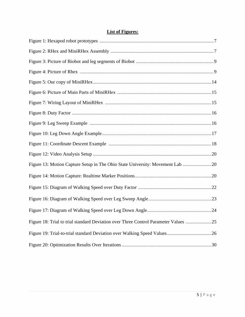
List of Figures:

Figure 1: Hexapod robot prototypes ....................................................................................................... 7

Figure 2: RHex and MiniRHex Assembly ............................................................................................. 7

Figure 3: Picture of Biobot and leg segments of Biobot ...................................................................... 9

Figure 4: Picture of Rhex ......................................................................................................................... 9

Figure 5: Our copy of MiniRHex ........................................................................................................... 14

Figure 6: Picture of Main Parts of MiniRHex ..................................................................................... 15

Figure 7: Wiring Layout of MiniRHex ................................................................................................ 15

Figure 8: Duty Factor .............................................................................................................................. 16

Figure 9: Leg Sweep Example .............................................................................................................. 16

Figure 10: Leg Down Angle Example ................................................................................................... 17

Figure 11: Coordinate Descent Example ............................................................................................. 18

Figure 12: Video Analysis Setup ........................................................................................................... 20

Figure 13: Motion Capture Setup in The Ohio State University: Movement Lab .......................... 20

Figure 14: Motion Capture: Realtime Marker Positions ..................................................................... 20

Figure 15: Diagram of Walking Speed over Duty Factor .................................................................. 22

Figure 16: Diagram of Walking Speed over Leg Sweep Angle ......................................................... 23

Figure 17: Diagram of Walking Speed over Leg Down Angle .......................................................... 24

Figure 18: Trial to trial standard Deviation over Three Control Parameter Values ....................... 25

Figure 19: Trial-to-trial standard Deviation over Walking Speed Values ........................................ 26

Figure 20: Optimization Results Over Iterations ................................................................................. 30

6 | P a g e

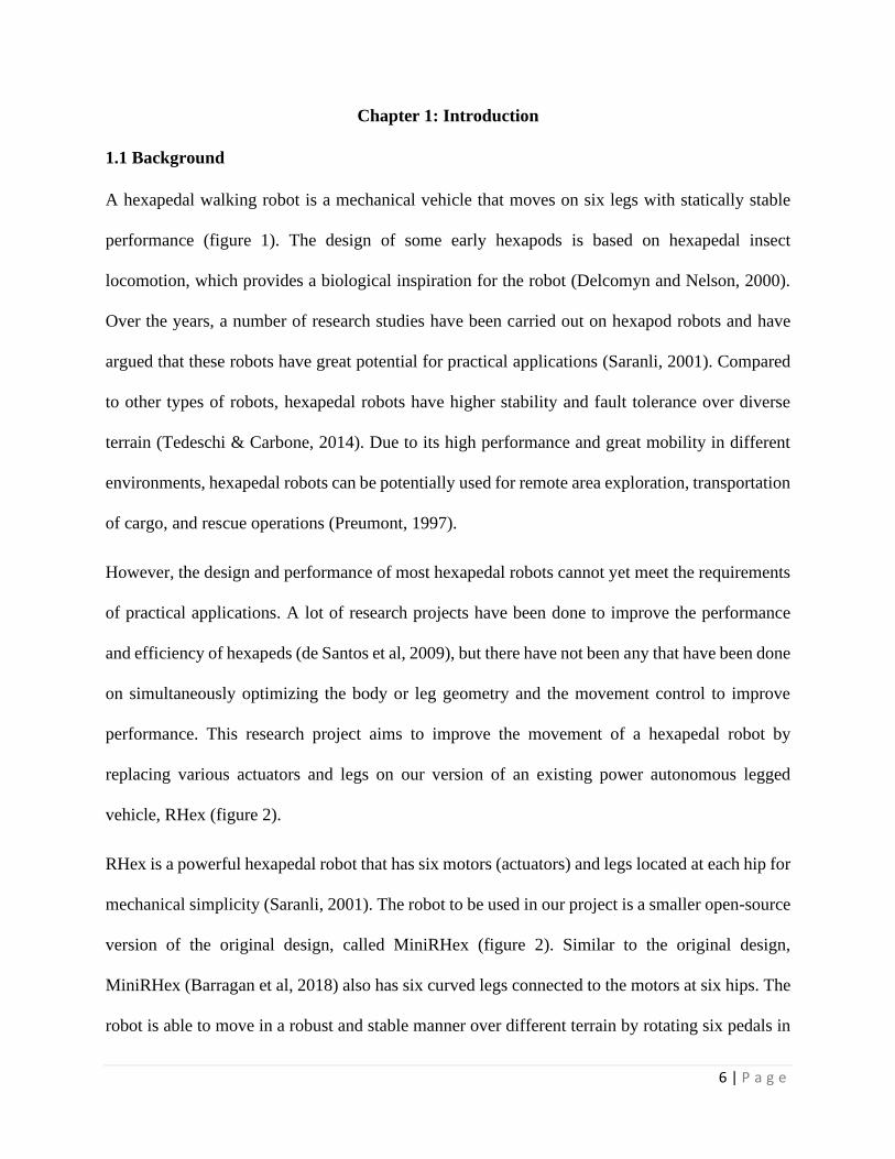
Chapter 1: Introduction

1.1 Background

A hexapedal walking robot is a mechanical vehicle that moves on six legs with statically stable

performance (figure 1). The design of some early hexapods is based on hexapedal insect

locomotion, which provides a biological inspiration for the robot (Delcomyn and Nelson, 2000).

Over the years, a number of research studies have been carried out on hexapod robots and have

argued that these robots have great potential for practical applications (Saranli, 2001). Compared

to other types of robots, hexapedal robots have higher stability and fault tolerance over diverse

terrain (Tedeschi & Carbone, 2014). Due to its high performance and great mobility in different

environments, hexapedal robots can be potentially used for remote area exploration, transportation

of cargo, and rescue operations (Preumont, 1997).

However, the design and performance of most hexapedal robots cannot yet meet the requirements

of practical applications. A lot of research projects have been done to improve the performance

and efficiency of hexapeds (de Santos et al, 2009), but there have not been any that have been done

on simultaneously optimizing the body or leg geometry and the movement control to improve

performance. This research project aims to improve the movement of a hexapedal robot by

replacing various actuators and legs on our version of an existing power autonomous legged

vehicle, RHex (figure 2).

RHex is a powerful hexapedal robot that has six motors (actuators) and legs located at each hip for

mechanical simplicity (Saranli, 2001). The robot to be used in our project is a smaller open-source

version of the original design, called MiniRHex (figure 2). Similar to the original design,

MiniRHex (Barragan et al, 2018) also has six curved legs connected to the motors at six hips. The

robot is able to move in a robust and stable manner over different terrain by rotating six pedals in

7 | P a g e

a certain algorithm (Altendorfer et al, 2001). In our project, we will improve the performance of

the robot moving with different legs by systematically changing the leg geometry such as length,

curvature, shape, and mass. The parameter sweep method and coordinate descent will be used in

the analysis to optimize the movement and determine the optimal leg shape and properties.

Figure 2: Left panel: RHex (Image from Boston Dynamics, n.d.). Right panel: MiniRHex

Assembly (Image from Barragan et al, 2018)

Figure 1: a) Cockroach is an inspiration for a hexapod robot. b-c) hexapod robot prototypes.

(Image from Delcomyn, 2000)

8 | P a g e

1.2 Purpose of Research

The objectives of this project are to:

• Utilize 3D printer and laser cutting to construct robot parts. Assemble the basic version of

the robot.

• Design various types of alternate leg components with CAD software such as Solidworks.

• Utilize motion capture to measure the movement of the robot. Perform parameter sweeps

to understand the effect of various parameters. Analyze motion data with MATLAB.

• Apply coordinate descent to optimize robot.

• Determine the robot body and control that maximizes the robot performance. Due to time

constraints, we revised our goals to examine only the optimization of movement control

parameters.

1.3 Literature Review

1.3.1 Existing Hexapod Prototypes

The design of most hexapods is initially based on hexapedal insect locomotion such as a cockroach

(figure 1). The robot shown in figure 3 is designed with insect-like keg structure and actuators that

mimic the movement of the American cockroach (Delcomyn, 2000). The research team that

develops this prototype model it after the cockroach because of its extraordinary speed and high

agility. Also, compared to other legged insects that have a more complicated structure and

movement algorithm, the structure and physiology of a cockroach are reasonably well known. The

robot has six actuators with six legs attached and the six legs are employed with three segments

each to mimic the insect. Each leg segment has a different length and structure.

9 | P a g e

The robot we are using in this project is called MiniRhex (Barragan et al, 2018) and it is a small

scaled version based on the Rhex hexapod. Different from some early prototypes introduced above,

Rhex has a unique and simple design. Rhex has only six actuators (motors) located at each hip

(figure 4). The legs rotate in a full circle with three legs in a group to push the robot forward. The

robot has strong mobility and maneuverability over diverse terrain (Saranli, 2001). The research

team conducted multiple tests to justify the high performance of Rhex on different surfaces (Table

1). The results indicate RHex has great potential in terms of maneuverability in various settings.

Figure 3: Picture of Biobot and leg segments of Biobot (Image from Delcomyn, 2000)

Figure 4: Picture of Rhex (Image from Saranli, 2001)

10 | P a g e

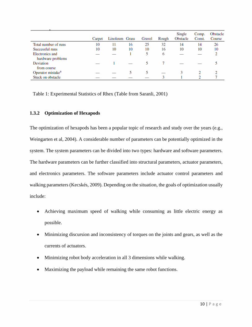
1.3.2 Optimization of Hexapods

The optimization of hexapods has been a popular topic of research and study over the years (e.g.,

Weingarten et al, 2004). A considerable number of parameters can be potentially optimized in the

system. The system parameters can be divided into two types: hardware and software parameters.

The hardware parameters can be further classified into structural parameters, actuator parameters,

and electronics parameters. The software parameters include actuator control parameters and

walking parameters (Kecskés, 2009). Depending on the situation, the goals of optimization usually

include:

• Achieving maximum speed of walking while consuming as little electric energy as

possible.

• Minimizing discursion and inconsistency of torques on the joints and gears, as well as the

currents of actuators.

• Minimizing robot body acceleration in all 3 dimensions while walking.

• Maximizing the payload while remaining the same robot functions.

Table 1: Experimental Statistics of Rhex (Table from Saranli, 2001)

11 | P a g e

The change of both hardware and software parameters will usually influence the optimal values of

other parameters (Silva, 2009). This means that these parameters are not independent parameters.

Trying out all the combinations of these parameters in experiments will be very time-consuming,

so the computer simulation is generally be used (Székács, 2013). In addition to hexapod-specific

optimization (Weingarten et al, 2004), there is a large and rapidly growing literature on robot-in-

the-loop optimization either using, for instance, reinforcement learning and direct optimization.

1.4 Significance of Research

Hexapod robots have great potential due to their high mobility and performance across diverse

terrain. These robots can be used in many fields such as remote area exploration, cargo

transportation, as well as surveillance and rescue missions. Various prototypes of hexapods have

been developed and studied by many researchers over the years, but the performance of most

hexapod prototypes have not met the requirement of practical use. One concern of the performance

is the relatively low walking speed. In order to improve performance, many control parameters

can potentially be optimized. The parameters are not independent, meaning that the change of one

parameter will affect the optimal value of the other. The research aims to co-optimize both

hardware and software parameters of a hexapod to improve the walking speed. The parameters

involved will be further explained in the methodology chapter. Whereas Weingarten et al, 2004

used the Nelder-Mead simplex method for hexapod optimization, here, we use a modified

coordinate descent, which appears to have not previously been used in this context.

12 | P a g e

Chapter 2: Methodology

2.1 Experiment Outline in Brief

The project’s objective is an optimization of the walking speed of a hexapod named MiniRhex.

Both control parameters and physical parameters are supposed to be considered in the optimization

process. Multiple optimization methods are supposed to be used during the process such as

parameter sweep and coordinate descent. The project consists of two parts, which are the

fabrication of the robot and the optimization of the performance. During fabrication, 3D printing

and laser cutting technologies are used to create leg and body components of the robot, all the

electrical components are purchased, and the robot assembled. For the optimization process,

motion capture will be used to measure the performance and analyze the data. For each trial, the

robot will be let to walking for 1 meter and the total travel time will be measured with motion

capture. Each trial will repeat at least 3 times and the average of the 3 numbers will be recorded to

reduce error.

2.2 Research Platform

2.2.1 Robot Details

The robot used in the experiment is MiniRHex developed by the Robomechanics Lab of Carnegie

Mellon University based on the hexapod RHex. The intention of designing this robot was to

provide an education or research platform for robot mechanics study. The low cost and simple

structure, as well as the high performance, are the main features of this robot (Barragan et al, 2018).

The comparison of MiniRhex and its full-sized prototype X-RHex are given in Table 2.

13 | P a g e

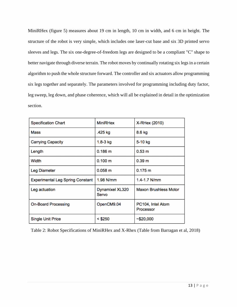
MiniRHex (figure 5) measures about 19 cm in length, 10 cm in width, and 6 cm in height. The

structure of the robot is very simple, which includes one laser-cut base and six 3D printed servo

sleeves and legs. The six one-degree-of-freedom legs are designed to be a compliant "C" shape to

better navigate through diverse terrain. The robot moves by continually rotating six legs in a certain

algorithm to push the whole structure forward. The controller and six actuators allow programming

six legs together and separately. The parameters involved for programming including duty factor,

leg sweep, leg down, and phase coherence, which will all be explained in detail in the optimization

section.

Table 2: Robot Specifications of MiniRHex and X-Rhex (Table from Barragan et al, 2018)

14 | P a g e

Part Number Weight (each)

Servo Sleeve 6 11g

Shaft-edge 4 3g

Shaft-mid 2 5g

Leg 6 2g

Battery Case 1 17g

2.2.2 Fabrication Details

The structure of MiniRHex mainly consists of one lacer cut base and six pairs of 3D printed servo

sleeves and legs. The full list main components and their mass are listed in Table 3. After acquiring

all the body components (figure 6), we made sure the size of holes fit the 3mm screws that is going

Figure 5: Our copy of MiniRHex that we fabricated at the Ohio State University

Table 3: Robot Part List (Barragan et al, 2018).

15 | P a g e

to use later. We then attached the servo motors into the sleeve parts first before fixing them on the

base. The next step is to install the six shafts on the servo motors and make sure shafts align the

servo motor correctly. Then, we installed the middle two legs onto the two middle long shafts first

before installing the other four legs. After installing all the structure components, we wired the

servo motors and the controllers as Figure 7 shows.

Figure 6: Picture of Main Parts of MiniRHex (Image from Barragan, 2018)

Figure 7: Wiring Layout of MiniRHex (Image from Barragan, 2018)

16 | P a g e

2.3 Optimization

2.3.1 Parameters

The optimization process of this project mainly focuses on improving the walking speed of the

robot. The walking speed is an important factor to evaluate the performance of the hexapod

walking robot. In order to optimize the walking speed, several parameters are considered in the

experiment. The robot control parameters include duty factor, leg sweep, leg down, and phase

coherence.

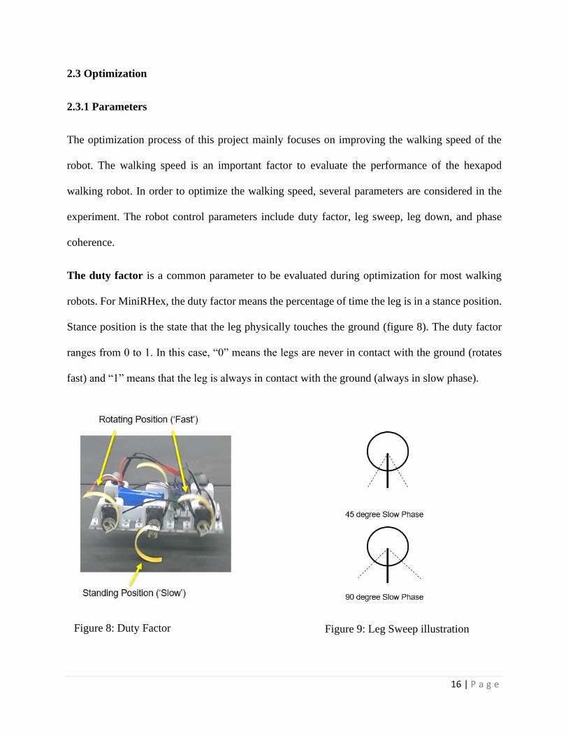
The duty factor is a common parameter to be evaluated during optimization for most walking

robots. For MiniRHex, the duty factor means the percentage of time the leg is in a stance position.

Stance position is the state that the leg physically touches the ground (figure 8). The duty factor

ranges from 0 to 1. In this case, “0” means the legs are never in contact with the ground (rotates

fast) and “1” means that the leg is always in contact with the ground (always in slow phase).

Figure 8: Duty Factor

Figure 9: Leg Sweep illustration

17 | P a g e

Leg sweep angle is an important parameter to be considered for MiniRhex particularly. Leg sweep

is defined as the angle width of stance position (“slow phase”) while walking (figure 9). Leg sweep

could range from 0 to 360 degrees, where 0 degree means there is no slow phase and 360 degrees

means entire rotation is in a slow phase. In the experiment, a reasonable range of 20 to 180 degrees

are chosen.

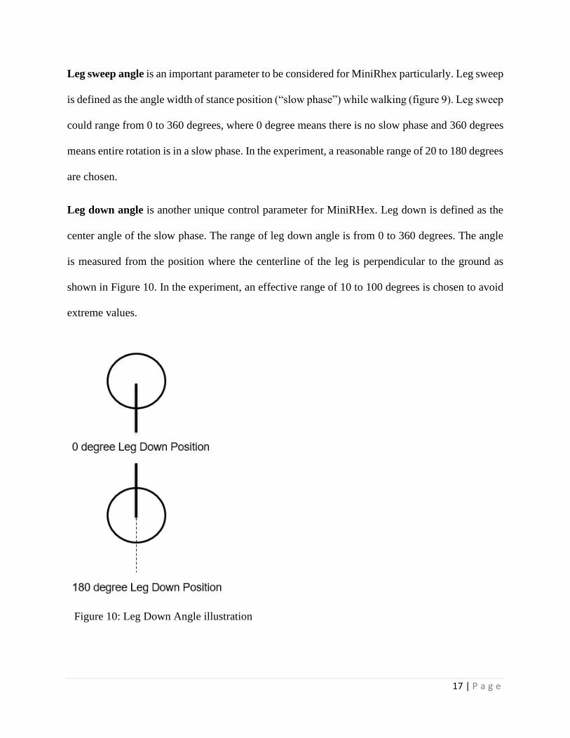
Leg down angle is another unique control parameter for MiniRHex. Leg down is defined as the

center angle of the slow phase. The range of leg down angle is from 0 to 360 degrees. The angle

is measured from the position where the centerline of the leg is perpendicular to the ground as

shown in Figure 10. In the experiment, an effective range of 10 to 100 degrees is chosen to avoid

extreme values.

Figure 10: Leg Down Angle illustration

18 | P a g e

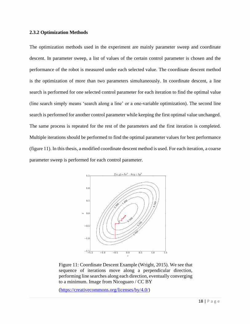
2.3.2 Optimization Methods

The optimization methods used in the experiment are mainly parameter sweep and coordinate

descent. In parameter sweep, a list of values of the certain control parameter is chosen and the

performance of the robot is measured under each selected value. The coordinate descent method

is the optimization of more than two parameters simultaneously. In coordinate descent, a line

search is performed for one selected control parameter for each iteration to find the optimal value

(line search simply means ‘search along a line’ or a one-variable optimization). The second line

search is performed for another control parameter while keeping the first optimal value unchanged.

The same process is repeated for the rest of the parameters and the first iteration is completed.

Multiple iterations should be performed to find the optimal parameter values for best performance

(figure 11). In this thesis, a modified coordinate descent method is used. For each iteration, a coarse

parameter sweep is performed for each control parameter.

Figure 11: Coordinate Descent Example (Wright, 2015). We see that

sequence of iterations move along a perpendicular direction,

performing line searches along each direction, eventually converging

to a minimum. Image from Nicoguaro / CC BY

(https://creativecommons.org/licenses/by/4.0/)

19 | P a g e

2.4 Experiment

2.4.1 Setup and Instrument

The reflective-marker-based motion capture and video-based analysis are two major methods for

motion data collection. Video analysis is mainly used in data collection for our parameter sweeps.

The speed of the robot is measured by looking at each frame of the video. During data collection,

the camera is fixed to include the robot as well as two lines that mark the length of one meter on

the ground (figure 12). The frame number is recorded as the front of the robot passes the “starting

line” mark and the “finish line” mark so that the total walking time can be calculated.

We intended to use 3D marker-based motion capture (Vicon Inc.) for coordinate descent data

collection. The coordinate descent requires the real-time robot performance data after each run, so

the video analysis is no longer viable. The motion capture collects the coordinate position of the

robot in real-time and streaming to PC, which allows real-time analysis of motion data (figure 13).

Four reflective markers are fixed to the MiniRHex and the two reflective dots are placed at the

starting point and endpoint respectfully (figure 14). The surrounding cameras capture the real-time

position of all the reflective markers. The motion data will be analyzed after each run to get the

performance.

Due to early lab closure on account of COVID-19, we were unable to have access to the motion

capture system. Therefore, we reverted to using stop-watch-based timing to estimate the speed of

the robot during the coordinate descent optimization. In the presence of mocap, we would have

used real-time capture of markers and adaptation of robot parameter values, all from a single

MATLAB program that also performed coordinate descent – so that the optimization process is

entirely automated except for returning the robot to the initial position on the treadmill.

20 | P a g e

Figure 12: Video Analysis Setup, showing start and finish lines in red.

Figure 13: Motion Capture Setup in The Ohio State University: Movement Lab

Figure 14: Motion Capture: Realtime Marker Positions

21 | P a g e

Chapter 3: Results and Discussion

3.1 Parameter Sweeps

In this section, we discuss the results of parameter sweep for univariate optimization. Parameter

sweeps are performed on all three control parameters, which include duty factor, leg sweep, and

leg down. Another important leg control parameter is the phase coherence and the experiment on

this parameter was performed by another undergraduate researcher at OSU’s Movement Lab

(Khan, 2019). Coordinate descent on selected control parameters is performed after the three-

parameter sweeps. The coordinate descent optimizes the three control parameters at the same to

find the optimal value for robot walking speed.

3.1.1 Optimization Results with Parameter Sweeps

The total walking time of the robot to walk for one meter is the key metric to determine the

performance in this optimization process. For each control parameter, a list of equally spaced

values with random order is generated within the range limit. The robot is set to run at least three

times with each value and the run times are recorded for calculation of walking speed. The default

values of the three parameters are: -- for blah, -- for blah, and – for blah. We keep two of the

parameters at their default values when we change the third.

For the duty factor parameter sweep, a list of values 8 values ranging from 0.10 to 0.65 are put in

random order and the robot is set to run under these values accordingly. The summarized results

are plotted with walking speed versus duty factor values (figure 15). For each duty factor, the mean

walking speed is labeled with a blue cross. The maximum speed and minimum speed (from the

three trials per parameter value) are labeled with dots with different colors. According to the

diagram, the top walking speed is 0.146 m/s at the minimum duty factor value of 0.10. As the value

22 | P a g e

of duty factor increases, the walking speed gradually decreases till the local minimum value of

0.037 m/s at a duty factor value of 0.56. The walking speed remains approximately the same after

that point. The duty factor is the percentage of time the leg is in standing position. By definition,

the leg rotation speed will increase as the duty factor value decrease. The walking speed is directly

associated with leg rotation speed. So, the walking speed will reach peak value with minimum

duty factor value.

For leg sweep parameter sweep, a list of values 8 values ranging from 20 to 180 degrees are put in

random order and the robot is set to run under these values accordingly. The results are summarized

by plotting walking speed versus the leg sweep values (figure 16). The labeling for the diagram is

similar to figure 15. According to the diagram, the top walking speed is 0.125 m/s at a maximum

leg sweep value of 180 degrees. As the value of the leg sweep angle increases, the walking speed

Figure 15: Diagram of Walking Speed over Duty Factor

23 | P a g e

gradually increases from a local minimum value of 0.041 m/s at a leg sweep angle of 20 degrees.

Recall that the leg sweep angle is the angular width of the slow phase during rotation. Given other

parameters remain unchanged, the time for one complete rotation should remain the same. Since

the angular width of the slow phase is increased, the leg rotation speed for the fast phase will

increase in order to control the time of each rotation.

The optimization for the leg down angle is similar to the previous two optimizations as well as the

notation of the diagrams. The list of random values of leg down ranged from 10 to 100 degrees are

chosen. According to figure 17, the walking speed reaches a maximum value of 0.129 m/s at the

leg down angle of 55 degrees. As the leg down angle increases, the average walking speed

increases almost linearly from a minimum value of 0.054 m/s to the peak value. Then the walking

speed slowly decreases to a steady value of approximately 0.120 m/s.

Figure 16: Diagram of Walking Speed over Leg Sweep Angle

24 | P a g e

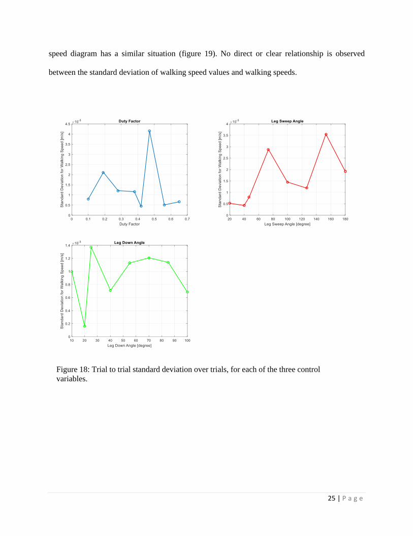
3.1.2 Trial to Trial Consistency

Trial to trial consistency is an important factor to determine if the data collection method and

performance of the robot are capable of repeated tests. In this experiment, the consistency is

evaluated based on the effect of walking speed and magnitude of control parameter values on the

standard deviation of measured data. For each trial, the data for a total number of three runs are

recorded. The standard deviations of the three walking speed values are calculated and plotted

against the corresponding parameter values (figure 18). The standard deviation for walking speed

in each trial is small compared to the speed values and its magnitude varies for different parameter

values. According to the diagram, no direct relationship between the standard deviation of walking

speed values and parameter values is overserved. The values of standard deviation are randomly

distributed across the range of all three control parameters. The standard deviation versus walking

Figure 17: Diagram of Walking Speed over Leg Down Angle

25 | P a g e

speed diagram has a similar situation (figure 19). No direct or clear relationship is observed

between the standard deviation of walking speed values and walking speeds.

Figure 18: Trial to trial standard deviation over trials, for each of the three control

variables.

26 | P a g e

3.2 Coordinate Descent

The coordinate descent method focuses on improving the walking speed by optimizing all three

control parameters mentioned above, which include duty factor, leg sweep angle, and leg down

angle. We used a ‘modified coordinate descent’ where instead of a local line search, we use a

global parameter search along with each control parameter. For each iteration, a list of N = 7

Figure 19: Trial-to-trial standard deviation over three trials per control parameter

value, plotted versus corresponding walking speed values. No trend is observed

with respect to the walking speed.

27 | P a g e

equally-spaced values is determined, spanning the range of all three parameters (table 4). One of

these values is chosen for each control variable: the robot is then set to run with these parameter

values and the walking time is recorded to calculate the walking speed of the robot. Then, we keep

two of the three control variables fixed, and change one variable through the N = 7 possibilities.

After running the robot with all the N values in the list, the value that gives the highest speed is

kept. The same process is repeated for each of the other two control variables while keeping the

other variables fixed. Each iteration will provide a list of optimal control parameter values. The

optimization process is complete when the robot walking speed can no longer be improved.

Trial Leg Down Angle Duty Factor Leg Sweep Angle

1 10.00 0.10 20.00

2 28.33 0.20 46.67

3 46.67 0.30 73.33

4 65.00 0.40 100.00

5 83.33 0.50 126.67

6 101.67 0.60 153.33

7 120.00 0.70 180.00

Table 4: List of Control Parameter Used

In the first coordinate descent we performed, starting from default values of the three parameters,

the optimization process takes only two iterations to converge, where convergence is defined as

two cycles yielding the same value. The first iteration results in a maximum speed of 0.1459 m/s

and the second iteration results in a maximum speed of 0.1468 m/s with the same parameter values

as in the first iteration (table 5). According to the data collected, the local optimal values for each

parameter are also the global optimal values. The values of the three control parameters that gives

the best performance are duty factor of 0.50, leg sweep angle of 46.67 degrees, and leg down angle

of 65.00 degrees The results of the optimization are close to the default settings (duty factor: 0.42,

leg sweep: 40, leg down: 20), suggesting that the default values were close to optimal.

28 | P a g e

Iteration 1

Initial parameter

values

Leg

down

Duty

factor

Leg

sweep

Speed

(m/s)

65.00 0.42 40.00 0.14098

What is changed

Leg

down

Duty

factor

Leg

sweep

Speed

(m/s)

Standard

deviation

Leg down 1 65.00 0.42 40.00 0.14098 0.001358

Leg down 2 101.67 0.42 40.00 0.13021 0.003683

Leg down 3 120.00 0.42 40.00 0.12793 0.001779

Leg down 4 28.33 0.42 40.00 0.10858 0.003427

Leg down 5 83.33 0.42 40.00 0.13010 0.003425

Leg down 6 10.00 0.42 40.00 0.06640 0.000108

Leg down 7 46.67 0.42 40.00 0.13333 0.004943

Duty factor 1 65.00 0.50 40.00 0.14225 0.000496

Duty factor 2 65.00 0.30 40.00 0.13630 0.004538

Duty factor 3 65.00 0.70 40.00 0.13889 0.000720

Duty factor 4 65.00 0.60 40.00 0.12341 0.004720

Duty factor 5 65.00 0.20 40.00 0.13316 0.003027

Duty factor 6 65.00 0.10 40.00 0.13544 0.001208

Duty factor 7 65.00 0.40 40.00 0.12386 0.003798

Leg sweep 1 65.00 0.50 73.33 0.01364 0.002946

Leg sweep 2 65.00 0.50 126.67 0.00789 0.002683

Leg sweep 3 65.00 0.50 100.00 0.01000 0.000285

Leg sweep 4 65.00 0.50 153.33 0.00652 0.002553

Leg sweep 5 65.00 0.50 180.00 0.00556 0.001500

Leg sweep 6 65.00 0.50 20.00 0.05000 0.002268

Leg sweep 7 65.00 0.50 46.67 0.14591 0.000503

Iteration 2

Initial parameter

values

Leg

down

Duty

factor

Leg

sweep

Speed

(m/s)

65.00 0.50 46.67 0.14684

What is changed

Leg

down

Duty

factor

Leg

sweep

Speed

(m/s)

Standard

deviation

Leg down 1 65.00 0.50 46.67 0.14684 0.001390

Leg down 2 101.67 0.50 46.67 0.12215 0.005420

Leg down 3 28.33 0.50 46.67 0.10733 0.001832

Leg down 4 120.00 0.50 46.67 0.12537 0.000924

29 | P a g e

Leg down 5 46.67 0.50 46.67 0.13717 0.004534

Leg down 6 83.33 0.50 46.67 0.13501 0.002053

Leg down 7 10.00 0.50 46.67 0.04437 0.001159

Duty factor 1 65.00 0.50 46.67 0.14684 0.004366

Duty factor 2 65.00 0.60 46.67 0.15940 0.005388

Duty factor 3 65.00 0.70 46.67 0.15213 0.005850

Duty factor 4 65.00 0.40 46.67 0.14265 0.001529

Duty factor 5 65.00 0.10 46.67 0.13953 0.001551

Duty factor 6 65.00 0.20 46.67 0.14634 0.004709

Duty factor 7 65.00 0.30 46.67 0.14677 0.001987

Leg sweep 1 65.00 0.50 153.33 0.13717 0.001414

Leg sweep 2 65.00 0.50 126.67 0.13514 0.000928

Leg sweep 3 65.00 0.50 46.67 0.14521 0.000865

Leg sweep 4 65.00 0.50 180.00 0.13280 0.004297

Leg sweep 5 65.00 0.50 100.00 0.14118 0.000656

Leg sweep 6 65.00 0.50 73.33 0.13993 0.001023

Leg sweep 7 65.00 0.50 20.00 0.13514 0.004919

Final result

Leg

down

Duty

factor

Leg

sweep

Speed

(m/s)

65.00 0.50 46.67 0.14521

Table 5: Coordinate Descent on Walking Speed Results. Version 1.

Perhaps because the initial guess of the previous coordinate descent is already close to the optimal

results, it only takes two iterations to converge. Seven values for each of the variables imply 73 =

147 combinations of parameters, whereas the two iterations only took about 44 parameter

combinations, making the algorithm more efficient than evaluating all parameter combinations.

In order to investigate the system more, another simplified version of previous coordinate descent

is performed starting with the worst parameter values from parameter sweeps. The new

optimization takes four iterations to converge and the results are summarized in Table 6. (Note

that this table records walking duration instead of walking speed.) In order to improve efficiency,

a total of four values instead of seven values are chosen for each parameter and the robot is set run

only one time per parameter set instead of using three trials per parameter set. Because we used

30 | P a g e

one trial instead of three to evaluate the speed for each parameter set, the random error per

evaluation may much higher. Due to this great uncertainty, the optimization method may not

converge as expected. One example is in iteration 2 trial 4, the parameter used in this trial is exactly

the same as the results from iteration 1, but the walking time value differs a lot, which may corrupt

the optimization process. A plot of all the walking time data over the iteration numbers is created

to show the trend of the optimization process (figure 20). The walking time duration (low speed)

starts a high value due to the bad parameter settings and the walking time ends at close to the

optimal values (as judged by our algorithm). Note that the two versions of the coordinate descent

arrived at close to the same forward speed, within 0.006 m/s of each other, compared to a speed

range 0.07 m/s during the optimization trials.

Figure 20: Coordinate descent, version 2. Optimization Results Over Iterations

31 | P a g e

Iteration 1

Initial parameter values

Leg down Duty factor Leg sweep Time (sec) Speed (m/s)

10.00 0.30 20.00 11.69 0.08554

What is changed

Leg down Duty factor Leg sweep Time (sec) Speed (m/s)

Leg down 1 10.00 0.30 20.00 11.69 0.08554

Leg down 2 83.33 0.30 20.00 7.22 0.13850

Leg down 3 46.67 0.30 20.00 7.19 0.13908

Leg down 4 120.00 0.30 20.00 7.10 0.14085

Duty factor 1 120.00 0.30 20.00 7.18 0.13928

Duty factor 2 120.00 0.50 20.00 7.78 0.12853

Duty factor 3 120.00 0.70 20.00 7.75 0.12903

Duty factor 4 120.00 0.10 20.00 6.63 0.15083

Leg sweep 1 120.00 0.10 20.00 6.90 0.14493

Leg sweep 2 120.00 0.10 126.67 7.53 0.13280

Leg sweep 3 120.00 0.10 73.33 7.06 0.14164

Leg sweep 4 120.00 0.10 180.00 10.38 0.09634

Iteration 2

Initial parameter values

Leg down Duty factor Leg sweep Time (sec) Speed (m/s)

120.00 0.10 20.00 6.90 0.14493

What is changed

Leg down Duty factor Leg sweep Time (sec) Speed (m/s)

Leg down 1 10.00 0.30 20.00 8.03 0.12453

Leg down 2 83.33 0.50 20.00 8.78 0.11390

Leg down 3 46.67 0.70 20.00 11.13 0.08985

Leg down 4 120.00 0.10 20.00 10.38 0.09634

Duty factor 1 10.00 0.50 20.00 7.82 0.12788

Duty factor 2 10.00 0.50 20.00 6.88 0.14535

Duty factor 3 10.00 0.50 20.00 8.19 0.12210

Duty factor 4 10.00 0.50 20.00 9.12 0.10965

Leg sweep 1 10.00 0.50 20.00 9.50 0.10526

Leg sweep 2 10.00 0.50 126.67 7.72 0.12953

Leg sweep 3 10.00 0.50 73.33 11.85 0.08439

Leg sweep 4 10.00 0.50 180.00 6.93 0.14430

Iteration 3

32 | P a g e

Initial parameter values

Leg down Duty factor Leg sweep Time (sec) Speed (m/s)

10.00 0.50 180.00 6.93 0.14430

What is changed

Leg down Duty factor Leg sweep Time (sec) Speed (m/s)

Leg down 1 10.00 0.50 180.00 6.94 0.14409

Leg down 2 83.33 0.50 180.00 7.47 0.13387

Leg down 3 46.67 0.50 180.00 6.91 0.14472

Leg down 4 120.00 0.50 180.00 6.97 0.14347

Duty factor 1 46.67 0.30 180.00 7.59 0.13175

Duty factor 2 46.67 0.50 180.00 7.12 0.14045

Duty factor 3 46.67 0.70 180.00 7.16 0.13966

Duty factor 4 46.67 0.10 180.00 11.35 0.08811

Leg sweep 1 46.67 0.50 20.00 7.06 0.14164

Leg sweep 2 46.67 0.50 126.67 7.38 0.13550

Leg sweep 3 46.67 0.50 73.33 6.84 0.14620

Leg sweep 4 46.67 0.50 180.00 6.90 0.14493

Iteration 4

Initial parameter values

Leg down Duty factor Leg sweep Time (sec) Speed (m/s)

46.67 0.50 73.33 6.84 0.14620

What is changed

Leg down Duty factor Leg sweep Time (sec) Speed (m/s)

Leg down 1 10.00 0.50 73.33 12.03 0.08313

Leg down 2 83.33 0.50 73.33 7.12 0.14045

Leg down 3 46.67 0.50 73.33 6.65 0.15038

Leg down 4 120.00 0.50 73.33 7.65 0.13072

Duty factor 1 46.67 0.30 73.33 7.47 0.13387

Duty factor 2 46.67 0.50 73.33 6.66 0.15015

Duty factor 3 46.67 0.70 73.33 6.88 0.14535

Duty factor 4 46.67 0.10 73.33 9.29 0.10764

Leg sweep 1 46.67 0.50 20.00 7.93 0.12610

Leg sweep 2 46.67 0.50 126.67 7.00 0.14286

Leg sweep 3 46.67 0.50 73.33 6.62 0.15106

Leg sweep 4 46.67 0.50 180.00 6.91 0.14472

Final Results

Leg down Duty factor Leg sweep Time (sec) Speed (m/s)

46.67 0.50 73.33 6.62 0.15106

Table 6: Coordinate Descent on Walking Time Results. Version 2.

33 | P a g e

3.3 Discussion

3.3.1 Limitations

The performance of the robot that is optimized in the project is the walking speed. Robot walking

speed is an important factor to determine the performance of hexapods, but other parameters such

as energy consumption, stability, and payload capacity are equally important. Only considering

the walking speed as the single factor to determine the robot's performance is not sufficient. In fact,

for a number of cases, the robot is not able to walk in a straight line or the robot base collides the

ground during walking are observed.

The optimization process is experiment-based, which means that the robot needs to be set to run

for every parameter change. For every single parameter, three walking data are recorded, and the

walking speed is calculated based on the average value of them. In order to minimize the operation

process, only 7 values are chosen for each control parameter, which may cause issues when

determining the optimal value. Increasing this grid size may improve the resolution up to which

the optimal value may be determined. With the current method, the optimal value is likely to appear

between two numbers in the list but the exact value cannot be determined. We may also consider

`grid refinement’ strategies, using a coarse grid initially and then a fine grid later on.

In the experiment, a modified coordinate descent optimization is conducted, which is a simplified

version of coordinate descent method. The optimal value is determined from the list of 7 or 8

values for each parameter based on the robot walking speed. The more accurate way is to fit the

best fit curve to the speed data over parameter values and then determining the local maximum of

that best-fit curve and repeat this in every direction. The optimal parameter value can be achieved

from the peak point, as well as the maximum walking speed.

34 | P a g e

Walking distance for both parameter sweeps and coordinate descent is set to be 1 meter. During

the experiment, the motors that actuate the legs do not work consistently. Multiple times of pause

and breaks are observed during the operation, especially under extreme parameter values. The

inconsistency will affect the actual performance of the robot significantly in a short distance. The

deviation for three runs in the trial as well as the trial to trial consistency will be influenced.

Note that the classical coordinate descent algorithm need not produce a global optimum, so the

solutions we obtained need to be considered to be likely local optima. One way to test (but not

prove) global optimality is to start the optimization from many initial seeds and see if they all

roughly converge to the same optimum.

3.3.2 Possible source of error

The performance data for parameter sweeps are measured with video analysis. The video of the

robot operating under various parameters is analyzed frame by frame to calculate the total run time.

The video has an FPS of 30 (30 frames per second) and sometimes may not be enough. The robot

may reach the end line between the frames and potential human error may affect the data collection.

Similar problems are also the cause of potential error during coordinate descent data collection.

Due to the limited access to motion capture instruments in the research lab, a stopwatch is used to

measure the walking time during coordinate descent. Human error may be involved in the process

and this random error can be minimized by collecting multiple trials of data. For such hand-timed

trials, systematic error may occur based on the human reaction time and may potentially affect the

results. It may be possible to estimate the random and systematic error in the human stop-watch-

based timing by comparing the human timing with video-based analysis, treating the latter as much

more accurate.

35 | P a g e

Hardware defects of the robot itself may affect the performance during operation, which also

causes the error. The center of gravity should be in the middle of the rectangle base of the robot to

ensure the balance during walking. The actual center of gravity is located slightly towards the back

of the base. The deviation of the center of gravity has little impact on the performance when the

robot is operating under parameters that close to default settings. However, the robot is observed

to lean to front and back under some values of the leg down angle. For instance, for some parameter

values, the robot body touches the ground, and this results in inconsistent walking time data. The

inconsistency in leg surface material and friction is another source of error. The robot legs are

made from 3D printing and the material is ABS plastic, which has low friction. In order to increase

the friction, a plastic spray is applied to each leg, but the plastic is not evenly distributed on the

surface of curved legs. The inconsistency of leg surfaces will stop the robot moving in a straight

line, which causes errors in data collection. Finally, another issue to contend with during such

optimization is the robot hardware properties slowly changing with time: for instance, wear of the

leg surfaces (which we do not believe is an issue here) and battery discharging over time. We did

not explicitly account for such slow changes in this work, although the battery was kept well-

charged during the trials.

36 | P a g e

Chapter 4: Conclusion and Future Work

The project consists of two parts: the assembly and fabrication of MiniRHex hexapods and the

robot walking speed optimization. The main body components of the robot including motor sleeves,

motor shafts, legs, and battery holds are 3D printed with ABS plastic. The base of the robot is

made from the acrylic board with lacer cutting. The optimization of walking speed is based on

parameter sweep and coordinate descent methods. The parameter sweeps are performed on duty

factor, leg down angle, and leg sweep width angle. Each parameter sweep gives a local maximum

walking speed and a local optimal parameter value, with fixed values of the other parameters.

Coordinate descent is the co-optimization of the three control parameters. In order to improve the

efficiency of the data collection process, a modified coordinate descent method is used in the

experiment. The results of the optimization are three optimal values of three control parameters

chosen from a list of 7 values for each parameter. The maximum walking speed is achieved under

the optimal parameter values.

The coordinate descent optimization can be made more efficient by automating the process as we

had originally planned and partially implemented. The motion capture, remote control treadmill,

and wireless code update are the key technologies to fully automate the optimization process. The

automation of the optimization process allows a much higher resolution of parameter lists. The

coordinate descent can be conducted for numbers of iterations until the results converge. More

control parameters can be optimized at the same time. Other optimization methods can be applied

to improve performance such as gradient descent. More control parameters may also be considered

in the optimization process such as phase coherence. The performance of the robot can be

measured in other ways. The energy consumption, robot walking stability, as well as the payload

capacity.

37 | P a g e

References

• Altendorfer, R., Moore, N., Komsuoglu, H., Buehler, M., Brown, H. B., McMordie, D.,

... & Koditschek, D. E. (2001). Rhex: A biologically inspired hexapod

runner. Autonomous Robots, 11(3), 207-213.

• de Santos, P. G., Garcia, E., Ponticelli, R., & Armada, M. (2009). Minimizing energy

consumption in hexapod robots. Advanced Robotics, 23(6), 681-704.

• Delcomyn, F., & Nelson, M. E. (2000). Architectures for a biomimetic hexapod

robot. Robotics and Autonomous Systems, 30(1-2), 5-15.

• Kecskés, I., Székács, L., Fodor, J. C., & Odry, P. (2013, July). PSO and GA optimization

methods comparison on simulation model of a real hexapod robot. In 2013 IEEE 9th

International Conference on Computational Cybernetics (ICCC) (pp. 125-130). IEEE.

• M. Barragan, N. Flowers, and A. M. Johnson. "MiniRHex: A Small, Open-source, Fully

Programmable Walking Hexapod". In Robotics: Science and Systems Workshop on

``Design and Control of Small Legged Robots'', Pittsburgh, PA, June 2018.

• Preumont, A., Alexandre, P., Doroftei, I., & Goffin, F. (1997). A conceptual walking

vehicle for planetary exploration. Mechatronics, 7(3), 287-296.

• Saranli, U., Buehler, M., & Koditschek, D. E. (2001). RHex: A simple and highly mobile

hexapod robot. The International Journal of Robotics Research, 20(7), 616-631..

• Silva, M., Barbosa, R., & Tenreiro Machado, J. A. (2009). Development of a genetic

algorithm for the optimization of hexapod robot parameters. In IASTED International

Conference Applied Simulation and Modelling (ASM 2009) (pp. 77-82).

• Tedeschi, F., & Carbone, G. (2014). Design issues for hexapod walking

robots. Robotics, 3(2), 181-206.

• Wright, S. J. (2015). Coordinate descent algorithms. Mathematical Programming, 151(1),

3-34.

• Weingarten, J. D., Lopes, G. A., Buehler, M., Groff, R. E., & Koditschek, D. E. (2004).

Automated gait adaptation for legged robots. In IEEE International Conference on

Robotics and Automation, 2004. Proceedings. ICRA'04. 2004 (Vol. 3, pp. 2153-2158).