Optimizing Inventory Policies in Process Networksunder Uncertainty

Pablo Garcia-Herrerosa, Anshul Agarwalb, John M. Wassickc, Ignacio E.Grossmanna,∗

aDepartment of Chemical Engineering, Carnegie Mellon University, Pittsburgh (PA), USAbThe Dow Chemical Company. Midland (MI), USAcThe Dow Chemical Company. Freeport (TX), USA

Abstract

We address the inventory planning problem in process networks under uncer-tainty through stochastic programming models. The scope of inventory planningrequires the formulation of multiperiod models to represent the time-varyingconditions of industrial process, but the multistage stochastic programming for-mulations are often too large to solve. We propose a policy-based approximationof the multistage stochastic formulation that avoids anticipativity by enforcingthe same decision rule for all scenarios. The proposed formulation includes thelogic modeling inventory policies, and it is used to find the parameters thatoffer the best expected performance. We propose policies for inventory plan-ning in process networks with arrangements of inventories in parallel and inseries. We compare the inventory planning strategies obtained from the policy-based formulation with the analogous two-stage approximation of the multistagestochastic program. Sequential implementation of both planning strategies inreceding horizon simulations show the advantages of the policy-based model,despite the increase in computational complexity.

Keywords: Inventory planning, Process network, Stochastic programming,Inventory policies, Receding horizon

1. Introduction

Inventory planning is a critical aspect of enterprise-wide optimization [16].Inventories are used in production and logistic networks to coordinate supplycycles and to mitigate the risks associated with uncertainty. The importanceof inventory management in industrial applications derives from the effect ofstockouts in the levels of customer satisfaction and the impact of stock in theeconomic balance of companies. Remarkably, the value of U.S. inventories was

∗Corresponding authorEmail address: grossmann@cmu.edu (Ignacio E. Grossmann )

Preprint submitted to Computers & Chemical Engineering November 7, 2015

estimated to be over $1,707 billion in December 2013 [50], and the opportunitycost ascribed to capital invested in inventories added up to $434 billion in 2012[54]. Therefore, the potential savings from stockout prevention and inventoryrelated cost offer a huge opportunity for optimization.

Many strategies have been proposed to manage inventories since Harris [17]introduced the Economic Order Quantity (EOQ) model in 1913. The EOQmodel was developed to balance ordering and holding cost for problems witha deterministic demand rate. Classical models for inventory management withuncertain demand include continuous-review (r,Q) policies and periodic-reviewbasestock policies; the main purpose of these models is to minimize the expectedcost of replenishment and stockouts, since complete satisfaction of uncertaindemand might be too expensive or impossible.

One of the main advantages of the classical models is that they prescribea policy for inventory management that is easy to implement. In fact, thesepolicies are often optimal under assumptions satisfied by simple inventory man-agement problems. Therefore, policies are in practice the method of choice toplan inventories in most industrial applications. However, the complexity ofproduction networks limits the suitability of the classical models for inventorymanagement in production processes. The main complications for inventoryplanning in process networks arise from the network topology, the limitationsin production capacity, and the multiple sources of uncertainty.

It is common practice in industry to allocate storage units at different stagesof the network in order to decouple the production of successive sections. Therole of inventory is to buffer temporal mismatches among supply availability,processing rates, and demand. In addition to the raw material and final prod-uct inventories that are used to hedge against external uncertainties, productionnetworks also include intermediate inventories that protect against the variabil-ity in processing rates. The importance of intermediate inventories resides intheir ability to reduce the interdependence of processing units, to delay theformation of bottlenecks, and to increase capacity utilization.

The interest for the control of intermediate inventories in production pro-cesses can be traced back to the work by Simpson [42] in the 1950’s. However,few methodologies have been proposed for inventory planning under uncertaintyin continuous process networks. In this article, we focus on developing stochasticprogramming formulations that leverage the nature of the inventory planningproblem. We propose a new approach that includes the logic of inventory policiesin a mathematical programming framework with the purpose of finding optimalpolicy parameters. The idea is to combine the advantages of logic-based mathe-matical programming with the pragmatism derived from inventory managementtheory. This approach for inventory optimization is completely novel and of-fers significant benefits for production planning in complex networks. We showthat using policies for inventory management in process networks has advan-tages over multistage or two-stage stochastic programing techniques. From themodeling perspective, policies offer an alternative way to avoid anticipativitythat can be used on arbitrary sets of scenarios. From the industrial perspective,policies are attractive because they are intuitive and easy to implement.

2

The reminder of the article is organized as follows. In Section 2, we re-view the publications that are most relevant to our work. Section 3 introducesthe inventory planning problem that we address. The method that we pro-pose to solve the problem and to evaluate the solutions is outlined in Section4. In Section 5, we present a motivating example that illustrates the partic-ularities of the stochastic inventory planning problem. Section 6 presents theoptimization model for single-echelon basestock policies. In Section 7 we revisitthe motivating example to compare the inventory plans obtained from differ-ent stochastic programming models. Section 8 presents a general model forstochastic inventory planning in process networks. Sections 9 and 10 proposepolicies for inventory planning in process networks with inventories in paralleland in series, respectively. In Section 11, we present a simulation approach toevaluate the performance of inventory planning strategies. Sections 12 and 13implement the proposed inventory planning models in two different examples.Finally, Section 14 presents the conclusions.

2. Literature review

Management of intermediate inventories has been addressed in the litera-ture of multi-echelon supply chains, which was initiated with the seminal workof Clark and Scarf [4]. They proved that basestock policies are optimal for theaverage cost of multi-echelon serial systems with stationary stochastic demand,convex cost function, and finite horizon. Later, Federgruen and Zipkin [12]demonstrated the optimality of basestock policies in the infinite horizon. A re-cursive algorithm to calculate optimal basestock levels in the serial and assemblymulti-echelon system with linear costs was developed by van Houtum and Zijm[52]. A simpler procedure yielding lower and upper bounds on the echelon costfunctions was developed by Shang and Song [40]; they also present a heuristicfor approximating optimal basestock levels that performs surprisingly well inpractice.

The derivation of optimal policies for inventory management in networkswith general topologies is a challenging task. The analysis of multi-echelon as-sembly systems presented by Rosling [36] showed that their optimal basestockpolicies can be obtained from an equivalent serial system. For multi-echelon dis-tribution systems, basestock policies have only been proved to be optimal underthe assumption that stockouts occur with equal probability at the downstreaminstallations [6]. Under this balancing assumption, optimality of basestock poli-cies has been proved for two-echelon systems [11, 12] and for multi-echelonsystems [5].

The application of multi-echelon basestock policies to supply chain design isbased on two models: guaranteed service-time and stochastic service-level. Theguaranteed service-time model strategically locates safety inventories to satisfythe maximum product requirements that installations are committed to satisfyduring their net lead time. The model was initially developed by Kimball [25]for a single-stage system, and implemented in serial systems by Simpson [42].Extensions of the guaranteed service-time model for safety stock placement in

3

assembly and distribution networks have been developed for bounded demands[15, 14] and for normally distributed demands [19, 20]. The alternative stochas-tic service-level model developed by Lee and Billington [29] locates inventoriesto offer prescribed service levels at the installations of a decentralized supplychain; basestock levels are obtained from the characterization of random delaysexperienced by installations as a result of shortages in the upstream stages.

Ettl et al. [8] developed expressions for the actual lead time in a multi-echelon supply chain by approximating the dynamics of inventory levels withqueuing models; they also included their inventory model in an optimizationframework to minimize the total inventory cost. The use of queuing modelsto characterize production and distribution networks started with the work ofJackson [21]. The advantage of queuing networks is that they allow modeling thedynamics of inventories in networks with finite processing capacity. The mostinfluential queuing models of manufacturing systems characterize them withproduct-form solutions that can be found for a restrictive class of networks, fromwhich Jackson networks are representative. An exceptional model capturing thedynamics of basestock policies in serial servers was developed by Lee and Zipkin[30]; they showed that the serial system can be described exactly for some specialcases and they developed approximations for the general case.

The characterization of optimal policies for capacitated production-inventorysystems with stationary demand was presented by Federgruen and Zipkin [9, 10].They showed that under the usual assumptions, a modified basestock policy isoptimal in the infinite horizon for the average and discounted cost criteria, andalso for the discounted cost criterion in a finite horizon. The modification of theclassic basestock policy accounts for the capacity limitation by truncating thereplenishment when the order-up-to quantity cannot be fulfilled. An algorithmto calculate optimal basestock levels and the corresponding costs for capacitatedmulti-echelon systems in the infinite horizon was developed by Tayur [47] usinga sequence of uncapacitated models that converge to the capacitated system.A more general simulation-based method to find optimal basestock levels incapacitated multi-echelon systems was presented by Glasserman and Tayur [13];their Infinitesimal Perturbation Analysis (IPA) estimates the sensitivity of thecost function with respect to the policy parameters and use them to recursivelyimprove the basestock levels.

Most of the literature about inventory management in chemical process net-works is related to deterministic systems. Karimi and Reklaitis [24] recognizedthe importance of intermediate storage for batch and semicontinuous processes,and derived expressions to find optimal storage capacities according to the pe-riodicity of the production processes. Other models for multiproduct batchplants have included uncertainty in the design problem [53, 39, 18], but theyhave not considered inventory management in their formulations. The inte-gration of batch plant design and scheduling was addressed by Subrahmanyamet al. [44] using a decomposition approach that iterates between a design su-perproblem and scheduling subproblems. Petkov and Maranas [33] addressedthe optimal design and operation of batch plants with normally distributeddemand for multiple products assuming a single-product campaign production

4

mode; they exploited the properties of normal distributions to find the optimaloperating policy corresponding to the potential designs.

Multi-echelon policies have also been applied for inventory management inthe process industry. Jung et al. [22] developed a simulation-optimization ap-proach in which safety stock levels are determined in a linear program andevaluated using discrete-event simulation. The proposed approach can accom-modate diverse network structures and uncertainty characterizations. Recently,Chu et al. [2, 3] presented a similar approach that uses agent-based simulationsto generate linear inequalities that are added to the LP planning problem toenforce the service level constraint; this approach has been used for reactivescheduling and multi-echelon inventory planning.

The guaranteed service-time model was implemented by You and Grossmann[56] for the design of chemical supply chains with uncertain demand; they ex-tended the guaranteed service-time methodology for production planning andinventory management in dedicated chemical networks that include capacityconstraints [57]. In a subsequent publication, dedicated and flexible processesare considered simultaneously by including a cyclic scheduling model that de-termines the sequence and duration of the flexible processes [58]. An MILPformulation for the optimal design of chemical networks with uncertainty insupply, demand, and random failures was developed by Terrazas-Moreno et al.[48, 49]. Their analysis considers the impact of slack production capacity andthe effect of intermediate inventories in the reliability of the production network.The formulation proposed by Terrazas-Moreno et al. [48] allows including diversecharacterizations of uncertainty as exemplified by their description of randomfailures using a Markov process.

An alternative approach for inventory management in production and dis-tribution networks has leveraged control theory for sequential decision-making.Bose and Pekny [1] proposed using Model Predictive Control (MPC) for plan-ning and scheduling of supply chain activities; their framework included forecast-ing, optimization, and simulation modules. Perea-Lopez et al. [31, 32] modeledthe dynamics of supply chains by considering flows of material and informa-tion. In a first article [31], they implemented site-dependent control laws tosimulate the behavior of decentralized supply chains in closed loop. In a secondarticle [32], they developed a discrete-time model of the supply chain dynamicsand used MPC to plan production and distribution in a rolling horizon. Theintegration of scheduling and control for coordination of production and dis-tribution has been recently addressed by Subramanian et al. [46]; their modelcharacterizes the state of the system according to inventory levels and comparethree MPC approaches that manipulate orders and shipments. In a related ar-ticle, Subramanian et al. [45] proposed a state-space model for scheduling thatdescribes the system with the levels of inventory, the tasks in progress, andtheir starting time; shipments, yield variations, delays, and unit breakdown areconsidered disturbances in the model.

Another body of literature related to our research advocates for the use ofstochastic programming in supply chain design and operation. Tsiakis et al. [51]proposed a MILP formulation for the design of multi-echelon supply chains con-

5

sidering scenarios with uncertain demand. You et al. [55] developed a two-stagestochastic programming model for supply chain planning under uncertainty withrisk management. Jung et al. [23] proposed a multistage stochastic program-ming formulation for multi-period supply chain planning; their solution methoditerates between a rolling horizon simulation and an outer loop that improvesthe safety stock targets using a gradient-based search.

Stochastic programming problems with a very large number of scenarioshave been successfully solved through Sample Average Approximation (SAA)[41, 26]. SAA is a framework to approximate the optimal expected value ofa stochastic program based on the solution of smaller problems with randomlysampled scenarios; the method provides statistical bounds on the expectation ofthe optimal objective value. Santoso et al. [37] implemented SAA for the optimaldesign of a supply chain with uncertain supply, capacity, cost structure, anddemand. The minimum-cost design of a supply chain with a complex topologywas formulated as a two-stage stochastic program by Schutz et al. [38]; in theirformulation, the design is decided in the first stage and the operation is modeledin the second stage. An implementation of SAA for the design of resilient supplychains was presented by Klibi and Martel [27]; their stochastic programmingformulation considers disruptions and other types of uncertainty in the scenarios.

3. Problem description

Inventory management involves decisions related to the replenishment anddepletion of inventories. In continuous process networks, inventory decisionsare closely related to production planning because most units are simultane-ously internal suppliers and consumers. The complexity of chemical productionnetworks requires storage of raw materials to guard against supply variability,intermediates to avoid the formation of bottlenecks, and final products to hedgeagainst demand uncertainty. The role of intermediate inventories is widely un-derstood in industrial applications but few methodologies have been proposedto optimize their management strategies in continuous process networks withcomplex topologies and capacity constraints.

This work addresses the inventory planning problem in continuous processnetworks with uncertainty in supply, available production capacity, and demand.We impose no restrictions on the characterization of the uncertain parametersother than the availability of discrete-time forecasts. Then, given a processnetwork with known structure, our goal is to propose planning strategies thatminimize the expected costs of inventory holding and stockouts in a finite hori-zon.

4. Outline of solution and result evaluation methods

The inventory planning problem under uncertainty can be formulated as astochastic programming (SP) problem where production and inventory decisionsare optimized to obtain the plan with minimum expected cost. In multiperiod

6

problems with a discrete number of scenarios, the optimal solution of such aproblem can be obtained by solving a multistage SP formulation. However,because of the computational difficulty to solve large-scale multistage SP models,it is often necessary to approximate them with two-stage SP formulations. Two-stage SP models are significantly easier to solve, but they do not capture thesequence in which information about uncertain parameters is revealed, whichmight deteriorate the quality of their solutions. We propose an alternativeapproximation of the multistage SP model that avoids anticipating the outcomesof uncertainty by enforcing inventory policies for all scenarios.

We develop a logic-based SP formulation that integrates inventory policiesin a mathematical programming framework. In order to optimize these policies,we first postulate a parametric model mapping the levels of inventory in thenetwork to replenishment and depletion actions. This parametric model is basedon the logic of basestock policies and includes additional rules according to thetopology of the process network. The logic-based SP formulation optimizes theparameters of the inventory policy with the objective of minimizing the expectedcost over the scenarios.

Each scenario describes the trajectory of all uncertain parameter through-out the planning horizon. The scenarios can be generated by reproducing allpossible trajectories in problems with discrete uncertain parameters, by simu-lating sample-paths from stochastic processes, from historical data, or from anyother forecasting method. The probability associated to scenarios depends onthe method used to generate them.

The most rigorous evaluation of the quality of a stochastic solution requirescomparing the expected cost obtained by implementing it with the optimal ex-pected cost of the multistage SP model. This is the approach that we followfor the motivating example in Sections 5 and 7. The alternative for prob-lems with too many scenarios is to compare different decision strategies usingclosed-loop Monte Carlo simulations. These simulations involve a sequentialdecision-making process that implements the first-period decisions recursively.The simulation horizon specifies the number of times that decisions are madeand implemented. Closed-loop Monte Carlos simulations yield a cost associatedwith the decision-making strategy, but this cost is a random outcome. There-fore, several replications are required to estimate the expected simulation costand to compare the quality of different decision-making strategies. We use thisapproach to evaluate the inventory planning strategies presented in Sections 9and 10.

5. A motivating example

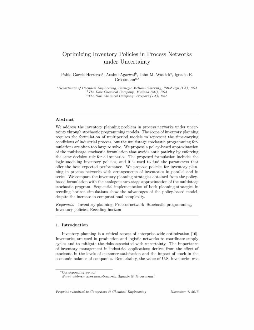
We present an small motivating example to illustrate the proposed inventoryplanning approach. The problem considers production planning and inventorymanagement in a production-inventory system with uncertain demand. Thesystem includes a single processing unit with deterministic production capacity,a storage unit with unlimited capacity, and stochastic demand. The planningproblem has a discrete time horizon with 11 periods spanning from t0 to t10.

7

Figure 1: Schematic representation of the motivating example.

Demands are independent and identically distributed (iid) uncertain parameterscharacterized by a discrete uniform probability distribution in periods t1 to t10.A schematic representation of the motivating example is presented in Fig. 1.

We consider the case study in which supply (S) is unlimited, available pro-duction capacity (C) is 100 units of product per period, and demand can beeither 110 or 90 units of product per period (DH = 110, DL = 90). It is worthnoticing that demand can be fully satisfied by accumulating inventory in theinitial time period (t0), even if the outcome of uncertain demand is high inperiods t1 to t10.

The objective of the planning problem is to minimize the expected costs as-sociated to inventory holding and stockouts. Stockouts are calculated accordingto the backorders model that carries out unsatisfied demands to the next timeperiod. We use a unit holding cost (H) of $5/unit-period and a unit backordercost (P ) of $15/unit-period.

The planning problem entails a sequential decision-making process in whichnew information becomes available as uncertainty is revealed with time. Theproblem has a discrete representation of time and a finite support for the un-certainty space; therefore, we can formulate it as a multistage SP problem. Themultistage SP model is presented in Eqns. (1)-(6).

min Hxt0 + Eξ∈Ξ

∑t∈T\{t0}

Hxξ,t + Pbξ,t

(1)

s.t. qξ,t + uξ,t = C ∀ t ∈ T, ξ ∈ Ξ (2)

8

[xξ,t − bξ,t] = [xξ,t−1 − bξ,t−1] + qξ,t −Dξ,t ∀ t ∈ T, ξ ∈ Ξ (3)

xξ,t = xξ′,t, bξ,t = bξ′,t, qξ,t = qξ′,t, uξ,t = uξ′,t

∀ t = {t0}, (ξ, ξ′) ∈ Ξ× Ξ (4)

xξ,t = xξ′,t, bξ,t = bξ′,t, qξ,t = qξ′,t, uξ,t = uξ′,t

∀ t ∈ T \ {t0}, (ξ, ξ′) ∈ Γt (5)

xξ,t, bξ,t, qξ,t, uξ,t ∈ R+ ∀ t ∈ T, ξ ∈ Ξ (6)

where T is the set of time periods (t), Ξ is the set of scenarios (ξ), and Γt isthe set of scenario pairs with the same outcomes of the uncertain parametersup to time t. This set is used to enforce that decisions can only depend on theoutcomes of past stages, which is the non-anticipativity condition. The formaldefinition of Γt for the example is given by Eqn. (7).

Γt :={

(ξ, ξ′) : (ξ, ξ′) ∈ Ξ× Ξ, (Dξ,t1 , Dξ,t2 , ..., Dξ,t) = (Dξ′,t1 , Dξ′,t2 , ..., Dξ′,t)}(7)

The multistage SP formulation given by Eqns. (1)-(6) is known as the ex-plicit representation because it includes copied variables for each scenario andNon-Anticipativity Constraints (NAC) relating them. The model denotes end-of-period inventory level with variables xξ,t and end-of-period stockouts withvariables bξ,t; processing rate is denoted with variables qξ,t and underutilizationwith uξ,t. The objective function is given by Eqn. (1). In the first period,t0, only holding cost is considered because there is no demand; in subsequentperiods, holding and backorder costs are incurred. Eqn. (2) represents the ca-pacity constraint of the processing unit, where the slack variable uξ,t denotesunderutilization. The mass balance in the storage unit is modeled with Eqn.(3); production in a period is considered instantaneous. Non-anticipativity ofthe decisions is enforced with Eqns. (5)-(4). The domains of the variables arepresented in Eqn. (6).

The multistage SP formulation for this motivating example describes in sce-narios the possible trajectories of demand; there are 1,024 scenarios correspond-ing to the sequences of demand from period t1 to t10. Despite the large numberof scenarios, this multistage SP model is a Linear Program (LP) that can besolved with any commercial solver. The optimal solution specifies the value of45,056 variables in the explicit representation or 8,188 variables in an implicitformulation without copied variables. However, the same optimal solution canbe described in much simpler form using a basestock policy.

The capacitated single-echelon basestock policy establishes rules to operatethe system according to the inventory level. The basestock level indicates theideal level of inventory in a given period. Following the basestock policy, pro-duction capacity and inventory are first used to satisfy demand; surplus capacityis used to intend replenishing inventory up to the basestock, but no inventory in

9

excess of the basestock level is hold. The optimal basestocks for the motivatingexample and the corresponding expected costs are presented in Table 1.

Period BasestockExpected costs [$]

Holding Backorder Total

t0 30 150.00 0.00 150.00t1 20 100.00 0.00 100.00t2 20 75.00 0.00 75.00t3 20 62.50 0.00 62.50t4 20 56.25 18.75 75.00t5 20 50.00 28.13 78.13t6 20 46.88 46.88 93.76t7 10 27.34 58.59 85.93t8 10 19.53 76.17 95.70t9 10 17.77 100.19 117.98t10 0 0.00 121.00 121.00

Total: 605.27 449.71 1,054.98

Table 1: Optimal basestock levels and costs for the motivating example.

6. Capacitated single-echelon basestock policy

It is not always easy to infer the optimal basestock levels from the solutionof the multistage SP formulation. Nevertheless, the simplicity and intuitiveappeal of inventory policies advocates for a general framework to obtain optimalbasestock levels. Let us denote by yt the basestock level of the single-echelonsystem at time t. Then, the sequence of events involved in implementation ofthe basestock policy can be described as follows:

1. Random demand (Dξ,t) is realized.

2. Production capacity (C) and carried over inventory (xξ,t−1) are used tosatisfy demand (Dξ,t) and backorders (bξ,t−1).

3. Surplus capacity is used to replenish inventory up to the basestock level(yt).

4. Inventory level (xξ,t) and backorders (bξ,t) are updated.

5. Holding or stockout cost is calculated.

The logic describing the operation of the basestock policy in a capacitatedsingle-echelon systems is simple. It can be characterized with the conditionsgiven by Eqns. (8)-(9).• Backorders (bξ,t) are allowed if there is no inventory:

bξ,t =

{0, if xξ,t > 0

Dξ,t + bξ,t−1 − xξ,t−1 − Ct, if xξ,t = 0(8)

10

• Underutilization (uξ,t) is allowed if inventory is at basestock level:

uξ,t =

{0, if xξ,t < yt

xξ,t−1 + C −Dξ,t − bξ,t−1, if xξ,t = yt(9)

In order to include the basestock policy in a mathematical programmingformulation, we divide the state-space of the system in three discrete states:empty inventory, intermediate level, and full inventory. In each state, the logicdictates the processing rate and inventory management plan according to adifferent rule. This logic can be modeled with the disjunctions presented inEqn. (10),

xξ,t = 0bξ,t ≥ 0uξ,t = 0

∨ 0 < xξ,t < yt

bξ,t = 0uξ,t = 0

∨ xξ,t = yt

bξ,t = 0uξ,t ≥ 0

∀ t ∈ T, ξ ∈ Ξ (10)

where the term on the left models the basestock policy with an empty inventory,the term on the center with an intermediate level, and the term on the right witha full inventory. Strict inequalities modeling intermediate levels (0 < xξ,t < yt)can be implemented in the mathematical programming environment with epsilonprecision (ε ≤ xξ,t ≤ yt − ε).

The formulation enforcing a basestock policy for inventory management inthe motivating example is obtained by replacing NAC constraints (5) with thelogic presented in Eqn. (10). The most obvious advantage of this logic-based SPformulation is that its solution can be easily characterized with the basestocklevels (yt). The formulation is a Generalized Disjunctive Program (GDP) thatcan be seen as a multiperiod SP formulation with piece-wise linear decision rulesfor inventory management [28].

The GDP model can be reformulated as a Mixed-Integer Linear Program(MILP) by introducing binary variables; for notational convenience, we denotebinary variables with a hat (ˆ) throughout the article. Binary variables x0

ξ,t

and xyξ,t indicate if the inventory is empty or at the basestock level, respectively.The conditions defining these variables are presented in Eqns. (11)-(14),

xξ,t ≤M(1− x0

ξ,t

)∀ ξ ∈ Ξ, t ∈ T (11)

xξ,t ≤ yt ∀ ξ ∈ Ξ, t ∈ T (12)

xξ,t ≥ yt −M(1− xyξ,t

)∀ ξ ∈ Ξ, t ∈ T (13)

x0ξ,t + xyξ,t ≤ 1 ∀ ξ ∈ Ξ, t ∈ T (14)

where the parameter M is an upper bound on the basestock level, Eqn. (11)forces the inventory to be empty if variable x0

ξ,t equals one, Eqns. (12)-(13)

forces the inventory to be at basestock level if x0ξ,t equals one, and Eqn. (14)

allows selecting only one of these states per scenario and time period.The logic presented in Eqn. (10) is completed with Eqns. (15)-(16),

11

bξ,t ≤M x0ξ,t ∀ ξ ∈ Ξ, t ∈ T (15)

uξ,t ≤M xyξ,t ∀ ξ ∈ Ξ, t ∈ T (16)

where Eqn. (15) allows stockouts only when the inventory is empty, and Eqn.(16) allows underutilization only when the inventory is at basestock level.

The MILP reformulation of the logic-based SP model is obtained by replacingthe NAC constraints (5) in the multistage SP model with Eqns. (11)-(16). Theresulting model can be solved using any available MILP solver.

7. Motivating example revisited

Despite the convenience of establishing production and inventory manage-ment plans according to a policy, solving the logic-based SP formulation canbe significantly harder than solving an LP model. Additionally, there is noguarantee that the optimal policy obtained from the logic-based SP formula-tion yields an expected value as good as the optimal multistage SP solution.However, large-scale multistage SP problems are also difficult to solve and oftenthe multistage model is only an approximation of the real problem. The mostcommon approximation is to restrict the number of scenarios in problems witha large number of discrete uncertain parameters or in problems with continuoussupport.

In order to asses the quality of the solutions obtained from different ap-proximations of multistage stochastic programs, we propose a new performancemetric called the Residual Expected Value (REV). The REV of a solution is theoptimal expected value of the multistage SP problem after fixing the first-stagevariables. The REV generalizes the multistage Value of the Stochastic Solution(VSS) to allow comparing the quality of different decision-making strategies,since VSS only compares the SP solution with the solution of the expectedvalue problem [7].

We evaluate the performance of a decision-making strategy by measuringhow much the REV deviates from the expected value obtained from the ex-act multistage SP formulation. Our analysis considers three decision-makingstrategies for the production and inventory planning problem presented in Sec-tion 5. All formulations approximate the multistage SP solution based on amodel with a reduced number of sampled scenarios. In addition to the multi-stage SP and the logic-based SP problem, we include in our analysis the resultsfrom the two-stage SP problem. The two-stage SP problem is obtained by re-laxing NAC constraints (5) of the multistage SP problem in all stages after thefirst. Instances of the scenario trees generated using the sampling technique arepresented in Fig. 2.

The trees presented in Fig. 2 are generated by sampling 10 scenarios ran-domly. The multistage structure in Fig. 2a can only be recognized in the first

12

(a) Sampled

multistage tree

(b) Sampled

policy-constraint tree

(c) Sampled two-stage

tree

Figure 2: Scenario trees for the motivating example

few periods. After period 5, the sampled multistage tree does not have indis-tinguishable scenarios, which makes it identical to the two-stage tree in Fig. 2c.On the other hand, the policy-constraint tree maintains non-anticipativity byimplementing a single decision logic for all scenarios.

We compare the REV for the three SP models using different sample sizes.Each point presented in Fig. 3 was estimated with 200 sample trees generatedusing Latin-Hypercubes Sampling; the same 200 sample trees were used to eval-uate all SP models. Fig. 3 shows that a relatively low number of scenarios isneeded to obtain a good first-stage solution with the multistage and logic-basedSP formulations; with 100 sample scenarios, both formulations produce a REVthat is within 1% of the expected value of the full multistage SP model. Thetwo-stage SP formulation on the other hand, does not seem to provide bettersolutions even with a larger number of scenarios; furthermore, the error bars in-dicate a high variability in its results. One of the most interesting observationsfrom Fig. 3 is that the logic-based SP formulation outperforms the multistageSP formulation when small sample sizes are used. This might be specially rele-vant for stochastic programming problems with a large number of scenarios orfor stochastic problems with continuous random parameters.

8. Mathematical model for stochastic inventory planning in processnetworks

Our model to formulate the inventory planning problem considers processnetworks of general topology. The transformation of raw materials into finalproducts is achieved with a sequence of steps that are carried out in specificprocessing units. We denote the set of materials by M and the set of processingunits by I. Three sets of parameters are considered uncertain in the formu-lation: available supply, available production capacity, and demand. For easeof notation, we use capitalized letters for parameters and sets, and lower-caseletters for variables and indexes; all variables in this section are defined in the

13

Figure 3: Residual expected value as a function of the sample size

positive real domain. The equations describing the mathematical model arepresented in the remainder of this section.

8.1. Supply balances

The availability of supply is modeled with Eqn. (17). The subset of materialsthat are externally supplied is denoted by MS . The amount of material m thatis available as external supply at time t and scenario ξ is given by parameterSξ,t,m. ISm is the subset of processing units that receive external supply ofmaterial m. The flow of supply consumed in unit i is denoted by fSξ,t,i,m, the

flow that is stored as inventory by rSξ,t,m, and the underutilization of supply byvξ,t,m.

Sξ,t,m =∑i∈ISm

fSξ,t,i,m + rSξ,t,m + vξ,t,m ∀ ξ ∈ Ξ, t ∈ T, m ∈MS (17)

8.2. Production capacity

The capacity of processing units is modeled with Eqn. (18). We definethe available production capacity (Cξ,t,i) as an uncertain parameter to modelrandom variations impacting the potential throughput of processing units; themaximum capacity of a unit is always greater than its available productioncapacity. The processing rate is denoted by qξ,t,i and the underutilization byuξ,t,i.

14

Cξ,t,i = qξ,t,i + uξ,t,i ∀ ξ ∈ Ξ, t ∈ T, i ∈ I (18)

8.3. Consumption balance

The consumption of material m in processing unit i is modeled with Eqn.(19). The subset of materials that are consumed in unit i is denoted by M in

i ; themass balance coefficient indicating the amount of material m that is consumedper unit production rate is give by parameter Ai,m. The subset of processingunits feeding material m to unit i is denoted by Iupi,m. The flow of material mfrom unit i′ to unit i is fξ,t,i′,i,m, and the amount of inventory depleted to feedunit i is modeled with variable dξ,t,i,m.

Ai,mqξ,t,i = fSξ,t,i,m +∑

i′∈Iupi,m

fξ,t,i′,i,m + dξ,t,i,m ∀ ξ ∈ Ξ, t ∈ T, i ∈ I, m ∈M ini

(19)

8.4. Production balance

The production of material m in processing unit i is modeled with Eqn.(20). The subset of materials that are produced in unit i is denoted by Mout

i ;the mass balance coefficient indicating the amount of material i that is producedper unit production rate is given by parameter Bi,m. The subset of processingunits receiving material m from unit i is denoted by Idowni,m . The amount ofinventory replenished by unit i is rξ,t,i,m, and the production flow that is usedto satisfy demand is fDξ,t,i,m.

Bi,mqξ,t,i =∑

i′∈Idowni,m

fξ,t,i,i′,m + rξ,t,i,m + fDξ,t,i,m ∀ ξ ∈ Ξ, t ∈ T, i ∈ I, m ∈Mouti

(20)

8.5. Inventory balance

The inventory of material m is modeled with Eqn. (21). The subset ofmaterials that can be stored is denoted by Mx. The balance includes the inven-tory carried-over from the last period (xξ,t−1,m), the replenishment from supply(rSξ,t,m), the replenishment from processing units (rξ,t,i,m), the inventory usedto feed processing units (dξ,t,i,m), and the inventory used to satisfy externaldemand (dDξ,t,m). The set of units allowed to replenish the inventory of materialm is denoted by Irm, and the set of units that can deplete inventory of materialm is denoted by Idm.

15

xξ,t,m = xξ,t−1,m + rSξ,t,m +∑i∈Irm

rξ,t,i,m −∑i∈Idm

dξ,t,i,m − dDξ,t,i,m

∀ ξ ∈ Ξ, t ∈ T, m ∈Mx (21)

8.6. Demand balance

Demand satisfaction is modeled with Eqn. (22). The subset of materialswith external demand is denoted by MD. Demand (Dξ,t,m) and carried-overbackorders (bξ,t−1,m) are equal to the production flow that is used satisfy de-mand (fDξ,t,i,m), the inventory that is depleted to satisfy demand (dDξ,t,m), andthe end-of-period backorders (bξ,t,m).

Dξ,t,m + bξ,t−1,m =∑i∈IDm

fDξ,t,i,m + dDξ,t,m + bξ,t,m ∀ ξ ∈ Ξ, t ∈ T, m ∈MD (22)

8.7. Objective function

Different objective functions can be used in the inventory planning problem.In our formulation, we minimize the sum of expected holding and stockout costsas presented in Eqn. (23). The probability of scenario ξ is denoted by Pξ. Theholding cost of material m at period t is denoted by Ht,m, and the penalty perunit backorder of material m at period t is denoted by Pt,m.

min∑ξ∈Ξ

Pξ∑t∈T

∑m∈Mx

Ht,mxξ,t,m +∑

m∈MD

+Pt,mbξ,t,m

(23)

9. Policy for inventories in parallel

We propose a priority-based policy for storable materials that compete forthe same replenishment resources. The basic condition is that policy parametersmust be the same across scenarios. The goal of the model is to establish theoptimal priorities (zn,l,m) and basestock levels (yt,m) for inventories in a paral-lel arrangement. An illustration of a parallel arrangement with three storablematerials is presented in Fig. 4.

16

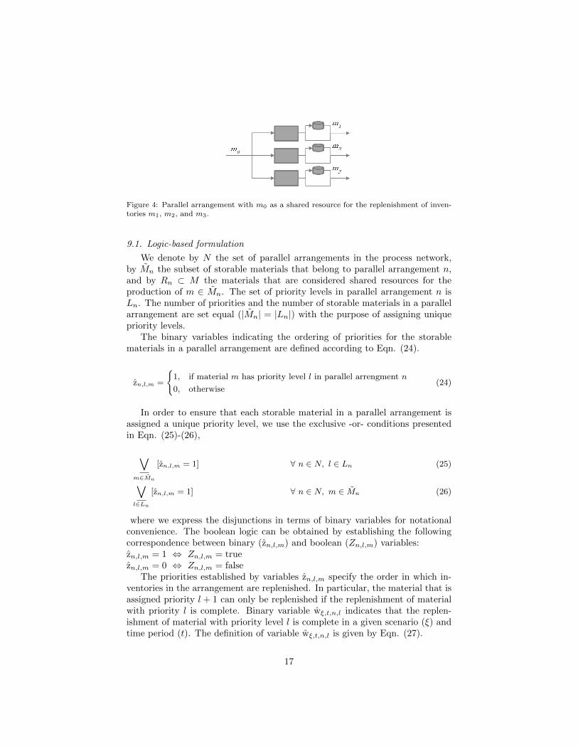
Figure 4: Parallel arrangement with m0 as a shared resource for the replenishment of inven-tories m1, m2, and m3.

9.1. Logic-based formulation

We denote by N the set of parallel arrangements in the process network,by Mn the subset of storable materials that belong to parallel arrangement n,and by Rn ⊂ M the materials that are considered shared resources for theproduction of m ∈ Mn. The set of priority levels in parallel arrangement n isLn. The number of priorities and the number of storable materials in a parallelarrangement are set equal (|Mn| = |Ln|) with the purpose of assigning uniquepriority levels.

The binary variables indicating the ordering of priorities for the storablematerials in a parallel arrangement are defined according to Eqn. (24).

zn,l,m =

{1, if material m has priority level l in parallel arrengment n

0, otherwise(24)

In order to ensure that each storable material in a parallel arrangement isassigned a unique priority level, we use the exclusive -or- conditions presentedin Eqn. (25)-(26),

∨m∈Mn

[zn,l,m = 1] ∀ n ∈ N, l ∈ Ln (25)

∨l∈Ln

[zn,l,m = 1] ∀ n ∈ N, m ∈ Mn (26)

where we express the disjunctions in terms of binary variables for notationalconvenience. The boolean logic can be obtained by establishing the followingcorrespondence between binary (zn,l,m) and boolean (Zn,l,m) variables:zn,l,m = 1 ⇔ Zn,l,m = truezn,l,m = 0 ⇔ Zn,l,m = false

The priorities established by variables zn,l,m specify the order in which in-ventories in the arrangement are replenished. In particular, the material that isassigned priority l + 1 can only be replenished if the replenishment of materialwith priority l is complete. Binary variable wξ,t,n,l indicates that the replen-ishment of material with priority level l is complete in a given scenario (ξ) andtime period (t). The definition of variable wξ,t,n,l is given by Eqn. (27).

17

wξ,t,n,l =

{1, if replenishment of material with priority l is complete

0, otherwise(27)

The completion of replenishment for material with priority level l impliesthat no additional upstream materials shared in the parallel arrangement areneeded to replenish this inventory. If we denote by Irm the set of units that canreplenish the inventory of material m, variable wξ,t,n,l must satisfy the conditiongiven by Eqn. (28).

zn,l,m = 1

xξ,t,m < yt,m∨i∈Irm

[uξ,t,i > 0

gξ,t,i,m = 0 ∀ m ∈M ini \ {Rn}

]

=⇒ wξ,t,n,l = 0 ∀ ξ ∈ Ξ, t ∈ T, n ∈ N, l ∈ Ln, m ∈ Mn (28)

The implication presented in Eqn. (28) states that the replenishment of in-ventory with priority level l cannot be considered complete if the inventory level(xξ,t,m) is below the basestock (yt,m), and there is available capacity (uξ,t,i > 0)and upstream materials (gξ,t,i,m = 0) for the units (i ∈ Irm) that can replen-ish it; we exclude the shared resource (Rn) from the set of upstream materials(M in

i ) required for the replenishment because their shortage does not relax theimplication. Binary variables gξ,t,i,m indicate if there is an upstream shortageof material m that does not allow increasing the processing rate in unit i. Thelogic establishing material shortage is given by Eqn. (29).

[xξ,t,m > 0] ∨ [vξ,t,m > 0]∨

i′∈Iupi,m

[uξ,t,i′ > 0

gξ,t,i′,m = 0 ∀ m ∈M ini′

]=⇒ gξ,t,i,m = 0 ∀ ξ ∈ Ξ, t ∈ T, i ∈ Iconsm , m ∈M (29)

Expression (29) does not allow indicating shortage of material m for theunits that consume it (i ∈ Iconsm ), if there is available inventory, supply under-utilization, or the upstream units capable of producing it (i′ ∈ Iupi,m) are not

fully utilized nor in shortage of the materials they consume (M ini ).

The priorities for the replenishment are enforced with Eqns. (30)-(31).

wξ,t,n,l = 0 =⇒ wξ,t,n,l+1 = 0 ∀ ξ ∈ Ξ, t ∈ T, n ∈ N, l ∈ Ln (30)∨l∈Ln

[zn,l,m = 1

wξ,t,n,l−1 = 0

]=⇒ rξ,t,i,m = 0

∀ ξ ∈ Ξ, t ∈ T, n ∈ N, i ∈ Irm, m ∈ Mn (31)

18

where Eqn. (30) guarantees that variables indicating the completion of replen-ishment (wξ,t,n,l) are activated following the order of priorities, and Eqn. (31)constraints replenishments according to the completion of levels that are hier-archically higher.

9.2. An MILP reformulation

We reformulate the logic for inventory management in parallel arrangementsusing mixed-integer constraints. The reformulation of constraints (25)-(26) isgiven by Eqns. (32)-(33).

∑m∈Mn

zn,l,m = 1 ∀ n ∈ N, l ∈ Ln (32)

∑l∈Ln

zn,l,m = 1 ∀ n ∈ N, m ∈ Mn (33)

The implication on replenishment completion (Eqn. (28)) can be reformu-lated according to Eqn. (34).

(1− zn,l,m) + xyt,m + u0ξ,t,i +

∑m′∈Min

i \Rn

gξ,t,i,m′ + (1− wξ,t,l) ≥ 1

∀ ξ ∈ Ξ, t ∈ T, n ∈ N, l ∈ Ln, i ∈ Irm, m ∈ Mn (34)

where binary variable u0ξ,t,i indicates if there is underutilization of unit i in

scenario ξ at time period t. We enforce the definition of u0ξ,t,i with the big-M

constraint presented in Eqn. (35).

uξ,t,i ≤M(1− u0

ξ,t,i

)∀ ξ ∈ Ξ, t ∈ T, i ∈ I (35)

The condition (29) that indicates shortage of upstream material m in unit ican be reformulated with Eqns. (36)-(39),

x0ξ,t,m + (1− gξ,t,i,m) ≥ 1 ∀ ξ ∈ Ξ, t ∈ T, i ∈ I, m ∈M (36)

v0ξ,t,m + (1− gξ,t,i,m) ≥ 1 ∀ ξ ∈ Ξ, t ∈ T, i ∈ I, m ∈M (37)

u0ξ,t,i′ +

∑m′∈Min

i′

gξ,t,i,m′ + (1− gξ,t,i,m) ≥ 1 (38)

∀ ξ ∈ Ξ, t ∈ T, i ∈ Iconsm , i′ ∈ Iupi,m, m ∈M (39)

where binary variable v0ξ,t,m indicates if there is supply underutilization of ma-

terial m in scenario ξ at time period t. We enforce the definition of v0ξ,t,m with

Eqn. (40),

19

vξ,t,m ≤M(1− v0

ξ,t,m

)∀ ξ ∈ Ξ, t ∈ T, m ∈MS (40)

Finally, the logic expressed in Eqns. (30)-(31) can be reformulated withEqns. (41)-(42), respectively.

wξ,t,n,l ≥ wξ,t,n,l+1 ∀ ξ ∈ Ξ, t ∈ T, n ∈ N, l ∈ Ln (41)∑i∈Irm

rξ,t,i,m ≤M (1− zn,m,l) +Mwξ,t,n,l−1

∀ ξ ∈ Ξ, t ∈ T, n ∈ N, l ∈ Ln,m ∈ Mn (42)

where the parameter M is an upper bound for the total replenishment from allunits i ∈ Irm.

It is important to remark that Eqns. (32)-(42) only represent one MILPreformulation of the logic developed for inventory management in parallel ar-rangements. Other reformulations with different number of variables and con-straints are possible; they might lead to stronger or weaker formulations withrespect to the LP relaxation.

10. Policy for inventories in series

The inventory planning for materials that undergo sequential transforma-tion is based on multi-echelon inventory theory. We identify from the networkstructure processing paths (k) starting at raw material nodes and finishing atend product nodes; the purpose is to coordinate inventory management for thematerials in these paths. A multi-echelon arrangement is a subset of storablematerials (Mk ⊆ Mx) associated with a particular processing path. We definean echelon as the subset (Mk,e ⊆ Mk) containing a number e of the most down-stream materials in multi-echelon arrangement Mk; echelons are numbered fromthe most downstream (echelon Mk,1) to the most upstream (echelon Mk,|EK |),according to the conventions from multi-echelon literature. An illustration ofthe echelons comprising a multi-echelon arrangement is presented in Fig. 5.

10.1. Logic-based formulation

Formally, the subsets of materials in echelon Mk,e is given by Eqn. (43),

Mk,e ={m : m ∈

{Mk,e−1 ∪mk,e

}}(43)

where mk,e is the storable material preceding other e−1 materials in processingpath k. Consequently, echelon Mk,1 only contains one final product (mk,1 ∈MD ∀ k ∈ K).

20

Figure 5: A multi-echelon arrangement with 3 echelons

The logic of basestock policies in multi-echelon systems is based on the con-cept of echelon inventory level. The echelon inventory level considers the avail-able inventory for all the materials that belong to the echelon. The challenge todefine the echelon inventory level in process networks is that materials changetheir identity through the production process; therefore, we have to consider themass balance coefficients (Ai,m and Bi,m) to calculate the equivalence betweenone material and its downstream successor. The inventory level (χξ,t,k,e) forechelons Mk,1 and Mk,e can be calculated from Eqns. (44)-(45), respectively.

χξ,t,k,1 = xξ,t,m − bξ,t,m ∀ ξ ∈ Ξ, t ∈ T, k ∈ K, m = mk,1 (44)

χξ,t,k,e =1

Qk,e,e−1χξ,t,k,e−1 + xξ,t,m

∀ ξ ∈ Ξ, t ∈ T, k ∈ K, e ∈ Ek\{e = 1}, m = mk,e (45)

where Qk,e,e−1 is the conversion ratio in the process that transforms materialmk,e into material mk,e−1 following processing path k. It is worth noticing thatthe inventory level of echelon Mk,1 includes backorders, and that our processdoes not consider in-transit inventory since the transportation between units isassumed to be instantaneous.

Based on the echelon inventory level, we can extend the capacitated single-echelon basestock policy for inventory planning in sequential production pro-cesses. The idea is to define basestock levels (yt,k,e) for each echelon, suchthat the available downstream inventory is considered in the replenishment de-cisions corresponding to material mk,e. The logic for capacity utilization of theunits (i ∈ Irm) that can replenish inventory xξ,t,m remains the same as in thesingle-echelon system, except that we now have to consider the case in which un-derutilization is forced because upstream material shortage. In a multi-echelonarrangement, the conditions allowing backorders and underutilization are givenby expressions (46)-(47), respectively.

21

χξ,t,k,1 > 0 =⇒ bξ,t,m = 0 ∀ ξ ∈ Ξ, t ∈ T, k ∈ K, m = mk,1 (46)

[χξ,t,k,e < yt,k,e] ∧ [gξ,t,m = 0 ∀ m ∈M ini ] =⇒ uξ,t,i = 0

∀ ξ ∈ Ξ, t ∈ T, k ∈ K, e ∈ Ek, i ∈ Irmk,e(47)

The equations defining echelon inventory levels (Eqns. (44)-(45)) and thelogic controlling production decisions (Eqns. (46)-(47)) can be used in a logic-based formulation to find the optimal parameters of the basestock policy. Forprocessing networks with multi-echelon arrangements, the parameters to opti-mize are the basestock levels for each echelon (yt,k,e).

10.2. A MILP reformulation

We reformulate the logic for inventory management in multi-echelon ar-rangements using mixed-integer constraints. Similarly to the capacitated single-echelon basestock policy, this reformulation requires variables that indicate thestate of the inventory level. We introduce binary variable χ0

ξ,t,k,1 indicating if

inventory in echelon 1 is empty, and variable and χyξ,t,k,e indicating if inventoryof echelon e is at basestock level. The definition for these variables is enforcedwith Eqns. (48)-(50).

χξ,t,k,1 ≤M(1− χ0

ξ,t,k,1

)∀ ξ ∈ Ξ, t ∈ T, k ∈ K (48)

χξ,t,k,e ≤ yt,k,e ∀ ξ ∈ Ξ, t ∈ T, k ∈ K, e ∈ Ek\{e = 1} (49)

χξ,t,k,e ≥ yt,k,e −M(1− χyξ,t,k,e

)∀ ξ ∈ Ξ, t ∈ T, k ∈ K, e ∈ Ek\{e = 1} (50)

The implication presented in Eqn. (46), preventing stockouts if inventory isavailable, can be reformulated with big-M constraint (51).

bξ,t,m ≤Mχ0ξ,t,k,1 ∀ ξ ∈ Ξ, t ∈ T, k ∈ K,m = mk,1 (51)

(52)

Finally, condition (47) can be reformulated with (47).

χyξ,t,k,e +∑

m∈Mini

gξ,t,i,m + u0ξ,t,i ≥ 1 ∀ ξ ∈ Ξ, t ∈ T, k ∈ K, e ∈ Ek, i ∈ Irmk,e

(53)

The MILP reformulation proposed for multi-echelon arrangements is ob-tained by enforcing Eqns. (44)-(45) together with Eqns. (48)-(53). The re-sulting reformulation is only one reformulation of the logic proposed for multi-echelon arrangements. Other reformulations are also possible.

22

11. Evaluating inventory planning strategies with closed-loop MonteCarlo simulations

In order to asses the potential benefits of implementing a policy-based pro-duction planning, we compare the planning decisions obtained by solving thelogic-based SP formulation with the decision obtained from the equivalent two-stage SP formulation. The challenge for large-scale problem is that the numberof scenarios in multiperiod problems grows exponentially; therefore, we cannotcalculate the REV exactly as we have done with the motivating example in Sec-tion 7. The alternative is to use the planning strategies in a receding horizonwith the purpose of simulating the sequential implementation of the decision-making process. The proposed closed-loop Monte Carlo simulations resembleEconomic MPC [34], but our focus is on finite planning horizons and we solvea stochastic programming problem at each time period.

The scenarios for the SP formulations represent possible values of the ex-ogenous uncertain parameters, from the current period until the end of theplanning horizon. We assume to have a probabilistic description of these pa-rameters, which allow us generating possible trajectories using sampling tech-niques. The multiperiod SP formulations with sampled scenarios can be con-sidered sample-path optimization problems [35]; the purpose of solving thesesample-path problems is to estimate the optimal planning strategy based on areduced set of scenarios.

Four different parameters must be specified for the implementation of theclosed-loop simulations: number of replications, length of the simulation hori-zon, length of the planning horizon, and sample size for the planning problem.The number of replications specifies how many closed-loop simulations we run;a large number of replications is desirable because it allows better estimationof the simulation expected cost and its variance. The simulation horizon is thelength of the simulation and specifies how many optimization problems we solvein each replication. The planning horizon is the length of the sample-paths usedas scenarios in the multiperiod formulations; it defines how far into the future welook when solving the planning problem. Finally, the sample size specifies howmany scenarios we include in the optimization problems; a larger the number ofscenarios tends to produce better approximations of the full problem, but thesample size is constrained by the computational complexity of the instances.

The closed-loop simulations are used to evaluate the performance of theproposed formulations for inventory and production planning. The procedure toestimate the expected performance of these planning strategies has the followingsteps:

1. Establish the parameters for the closed-loop simulations.

2. Start a closed-loop simulation (t∗ = 1).

2.1. Observe the state at simulation time (t∗).

2.2. Generate scenarios by randomly sampling paths of the exogenousuncertain parameters.

23

2.3. Formulate and solve the stochastic optimization problem.

2.4. Implement the decisions corresponding to the current simulation time(t∗).

2.5. Randomly generate the realizations of the exogenous uncertain pa-rameters for the next time period in the simulation (t∗ + 1).

2.6. Roll the simulation time forward (t∗ = t∗ + 1).

2.7. If simulation time is less than the simulation horizon, go back to Step2.1. Otherwise, continue to Step 3.

3. If the number of closed simulations is less than the number of replications,go back to Step 2. Otherwise, continue to Step 4.

4. Calculate the statistics over all replications and terminate.

Fig. 6 shows the trajectory of uncertain parameters in a closed-loop MonteCarlo simulation, where the past is represented by a unique path and the futureis represented by alternative paths indicating possible scenarios. The simulationpresented in Fig. 6 is performed over five periods (t∗ = 0 to t∗ = 4). At eachperiod, a stochastic SP problem with a 4-period planning horizon is solved.Then, time moves forward and uncertainty is revealed.

Figure 6: Trajectory of uncertain parameters in a closed-loop Monte Carlo simulation.

In the following examples, we compare the performance of the planningdecisions obtained from the logic-based SP formulations and the equivalent two-stage SP formulations. For both of them, we use exactly the same sampledscenarios in every instance. In addition, we use the same realizations of the

24

uncertain parameters in the implementation of the closed-loop simulations. Themathematical models and the sampling procedure are implemented in AIMMS4.8.3; all optimization problems are solved using GUROBI 6.0.0 on an Intel Corei7 CPU 2.93 Ghz processor with 4 GB of RAM.

12. Example with inventories in parallel

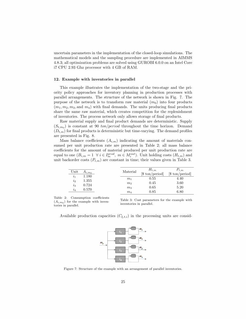
This example illustrates the implementation of the two-stage and the pri-ority policy approaches for inventory planning in production processes withparallel arrangements. The structure of the network is shown in Fig. 7. Thepurpose of the network is to transform raw material (m0) into four products(m1,m2,m3, and m4) with final demands. The units producing final productsshare the same raw material, which creates competition for the replenishmentof inventories. The process network only allows storage of final products.

Raw material supply and final product demands are deterministic. Supply(St,m0) is constant at 90 ton/period throughout the time horizon. Demand(Dt,m) for final products is deterministic but time-varying. The demand profilesare presented in Fig. 8.

Mass balance coefficients (Ai,m) indicating the amount of materials con-sumed per unit production rate are presented in Table 2; all mass balancecoefficients for the amount of material produced per unit production rate areequal to one (Bi,m = 1 ∀ i ∈ Iprodm , m ∈Mout

i ). Unit holding costs (Ht,m) andunit backorder costs (Pt,m) are constant in time; their values given in Table 3.

Unit Ai,m0

i1 1.180i2 1.355i3 0.724i4 0.570

Table 2: Consumption coefficients(Ai,m0 ) for the example with inven-tories in parallel.

MaterialHt,m Pt,m

[$ ton/period] [$ ton/period]

m1 0.55 4.40m2 0.45 3.60m3 0.65 5.20m4 0.85 6.80

Table 3: Cost parameters for the example withinventories in parallel.

Available production capacities (Cξ,t,i) in the processing units are consid-

Figure 7: Structure of the example with an arrangement of parallel inventories.

25

Figure 8: Deterministic demands for the example with inventories in parallel.

ered uncertain. Each uncertain parameter is modeled as an independent time-homogeneous Discrete Time Markov Chain (DTMC) with the purpose of de-scribing the state-dependent evolution of uncertainty in industrial processes.The states of the DTMCs characterize the value of the uncertain parameters;each parameter has three states that imply different available production capac-ities. Table 4 shows the value of each uncertain parameter according to theirstate.

ParameterState

Low Nominal High

Cξ,t,i1 13.23 14.70 16.17Cξ,t,i2 32.13 35.70 39.27Cξ,t,i3 22.68 25.20 27.72Cξ,t,i4 28.35 31.50 34.65

Table 4: Production capacities according to their DTMC state for the example with inventoriesin parallel.

We assume that all uncertain parameters are initially at their nominal values.The evolution of each DTMCs is characterized with the one-step transitionmatrix (Π). The same transition matrix is used to model the evolution of allproduction capacities. The transition matrix is given by Eqn. (54).

Low Nominal High

Π =

0.70 0.25 0.050.15 0.70 0.150.05 0.25 0.70

LowNominalHigh

(54)

It is worth noticing that in a single time period, there are 4 uncertain pa-rameters with 3 possible outcomes, giving rise to 81 possible combinations. Ina multiperiod problem with 6 time periods there are millions (816) of possible

26

scenarios, which would result in an intractable optimization problem for anypractical purpose.

We compare performance of the two-stage SP and the logic-based SP in-ventory planning strategies based on 25 closed-loop simulations. At eachperiod, each strategy solves a stochastic optimization problem with 10 sampledscenarios and a planning horizon of 6 time periods. In the logic-based SPformulation, we enforce the priority policy for the parallel arrangement madeup by the four final products (M1 = {m1,m2,m3,m4}) in planning periods 2,3, 4, and 5. It is unnecessary to enforce the policy in the first planning periodbecause the uncertainty has already been revealed; enforcing the policy in thelast planning period does not bring any benefit because no future periods canbe anticipated. The length of the simulation horizon is set to 12 periods.

Table 5 presents the computational statistics for the two-stage SP formula-tion and the MILP reformulation of the logic-based SP model. The number ofvariables and constraints remain the same throughout the simulations becausewe use a receding horizon approach. All MILPs are solved to an optimality gapof 0.25%.

StatisticFormulation

Two-stage SP Logic-based SP

Constraints: 1,812 4,204Continuous variables: 2,460 2,484Binary variables: 0 976Instances solved to optimality: 300 300Mean CPU time of instances [s]: < 1 176 (± 501)

Table 5: Computational statistics of the two-stage SP and the logic-based SP formulationsfor the example with inventories in parallel.

Table 5 shows a significant difference in computational complexity of bothmodels. It is important to remark that the two-stage SP formulation is strictlya relaxation of the logic-based SP formulation, and it has only a subset of thevariables and constraints. As a consequence, the mean CPU time required tosolve the instances of the two-stage SP model is less than one second; the meanCPU time for the instances of the logic-based SP model is 176 seconds, with astandard deviation of 501 seconds.

The results of the closed-loop simulations can be observed in Figs. 9-10,where the shaded lines represent the cost trajectories for the individual replica-tions and the solid lines are the averages over all replications. The figures showsimilar costs for both approaches, with a slightly higher stockout cost for thetwo-stage SP model that can be observed in periods 10 and 11. The trajectoriespresented in Figs. 9-10 evidence significant variability in the results obtainedfrom the implementation of both planning strategies. This variability is inher-ent to the nature of the problem, because uncertainty in production capacitiesconstitutes a high risk for stockouts. The main performance metric for the plan-ning strategies is the expected cost of simulations. Table 6 presents the meancost for each planning strategy over all simulations, together with its standard

27

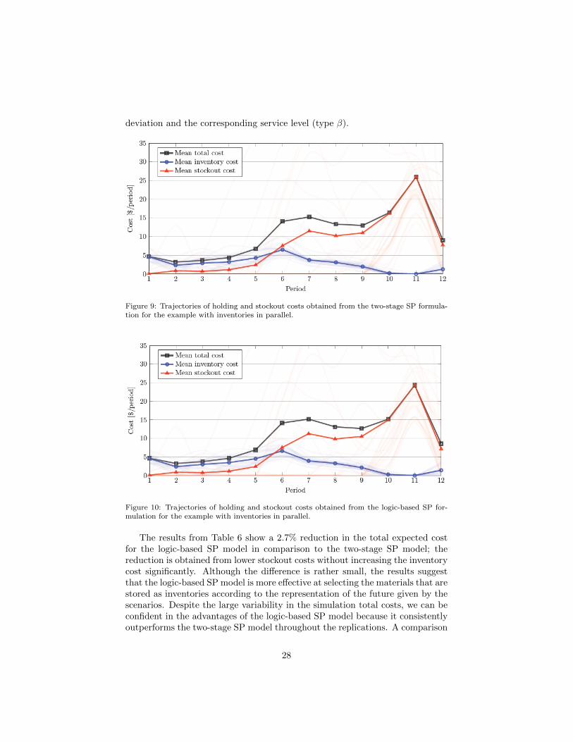
deviation and the corresponding service level (type β).

Figure 9: Trajectories of holding and stockout costs obtained from the two-stage SP formula-tion for the example with inventories in parallel.

Figure 10: Trajectories of holding and stockout costs obtained from the logic-based SP for-mulation for the example with inventories in parallel.

The results from Table 6 show a 2.7% reduction in the total expected costfor the logic-based SP model in comparison to the two-stage SP model; thereduction is obtained from lower stockout costs without increasing the inventorycost significantly. Although the difference is rather small, the results suggestthat the logic-based SP model is more effective at selecting the materials that arestored as inventories according to the representation of the future given by thescenarios. Despite the large variability in the simulation total costs, we can beconfident in the advantages of the logic-based SP model because it consistentlyoutperforms the two-stage SP model throughout the replications. A comparison

28

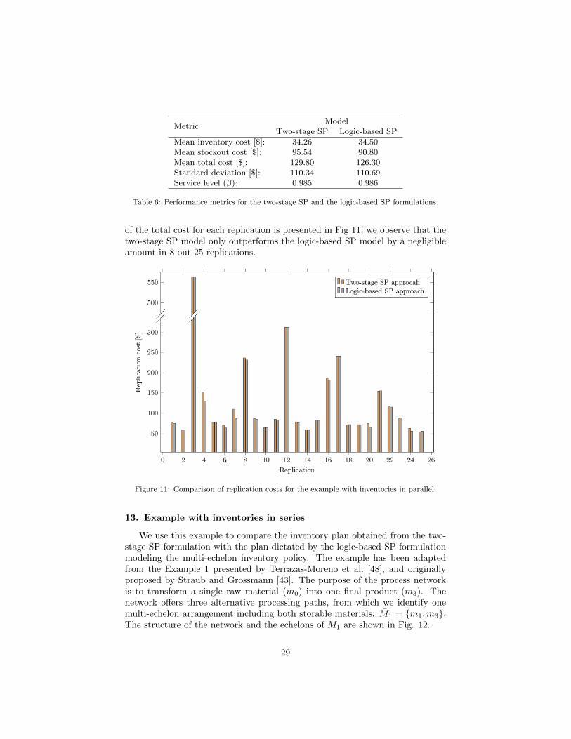
MetricModel

Two-stage SP Logic-based SP

Mean inventory cost [$]: 34.26 34.50Mean stockout cost [$]: 95.54 90.80Mean total cost [$]: 129.80 126.30Standard deviation [$]: 110.34 110.69Service level (β): 0.985 0.986

Table 6: Performance metrics for the two-stage SP and the logic-based SP formulations.

of the total cost for each replication is presented in Fig 11; we observe that thetwo-stage SP model only outperforms the logic-based SP model by a negligibleamount in 8 out 25 replications.

Figure 11: Comparison of replication costs for the example with inventories in parallel.

13. Example with inventories in series

We use this example to compare the inventory plan obtained from the two-stage SP formulation with the plan dictated by the logic-based SP formulationmodeling the multi-echelon inventory policy. The example has been adaptedfrom the Example 1 presented by Terrazas-Moreno et al. [48], and originallyproposed by Straub and Grossmann [43]. The purpose of the process networkis to transform a single raw material (m0) into one final product (m3). Thenetwork offers three alternative processing paths, from which we identify onemulti-echelon arrangement including both storable materials: M1 = {m1,m3}.The structure of the network and the echelons of M1 are shown in Fig. 12.

29

Figure 12: Structure of the example with a multi-echelon arrangement of inventories.

Supply availability (Sξ,t,m0), available production capacities (Cξ,t,i), and

demand are considered uncertain. Supply and demand are modeled as normallydistributed random variables; their mean values (Sξ,t,m0

, Dξ,t,m3) are periodic

functions presented in Fig. 13; their coefficients of variation are set to 15%.

Figure 13: Time-varying normally distributed supply and demand for the example with in-ventories in series.

The capacity (Cξ,t,i) of each processing unit is modeled as an independenttime-homogeneous Discrete Time Markov Chain (DTMC) with the purpose ofdescribing probabilistic failures. The DTMCs characterize the states of the unitsthat can be either working normally (up) or failed (down). Table 7 shows thevalue of production capacities according to their state.

30

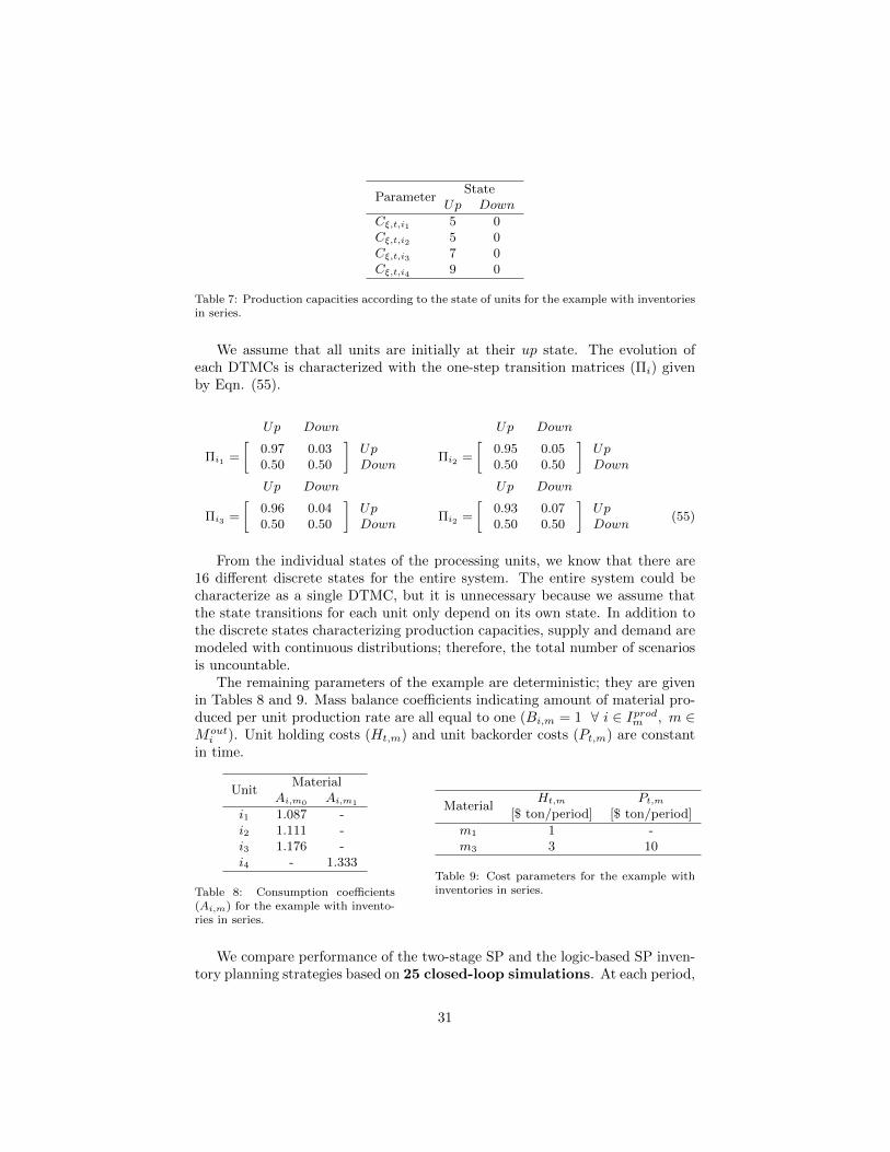
ParameterState

Up Down

Cξ,t,i1 5 0Cξ,t,i2 5 0Cξ,t,i3 7 0Cξ,t,i4 9 0

Table 7: Production capacities according to the state of units for the example with inventoriesin series.

We assume that all units are initially at their up state. The evolution ofeach DTMCs is characterized with the one-step transition matrices (Πi) givenby Eqn. (55).

Up Down Up Down

Πi1 =

[0.97 0.030.50 0.50

]UpDown

Πi2 =

[0.95 0.050.50 0.50

]UpDown

Up Down Up Down

Πi3 =

[0.96 0.040.50 0.50

]UpDown

Πi2 =

[0.93 0.070.50 0.50

]UpDown

(55)

From the individual states of the processing units, we know that there are16 different discrete states for the entire system. The entire system could becharacterize as a single DTMC, but it is unnecessary because we assume thatthe state transitions for each unit only depend on its own state. In addition tothe discrete states characterizing production capacities, supply and demand aremodeled with continuous distributions; therefore, the total number of scenariosis uncountable.

The remaining parameters of the example are deterministic; they are givenin Tables 8 and 9. Mass balance coefficients indicating amount of material pro-duced per unit production rate are all equal to one (Bi,m = 1 ∀ i ∈ Iprodm , m ∈Mouti ). Unit holding costs (Ht,m) and unit backorder costs (Pt,m) are constant

in time.

UnitMaterial

Ai,m0 Ai,m1

i1 1.087 -i2 1.111 -i3 1.176 -i4 - 1.333

Table 8: Consumption coefficients(Ai,m) for the example with invento-ries in series.

MaterialHt,m Pt,m

[$ ton/period] [$ ton/period]

m1 1 -m3 3 10

Table 9: Cost parameters for the example withinventories in series.

We compare performance of the two-stage SP and the logic-based SP inven-tory planning strategies based on 25 closed-loop simulations. At each period,

31

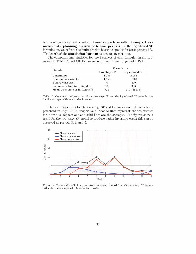
both strategies solve a stochastic optimization problem with 10 sampled sce-narios and a planning horizon of 5 time periods. In the logic-based SPformulation, we enforce the multi-echelon basestock policy for arrangement M1.The length of the simulation horizon is set to 15 periods.

The computational statistics for the instances of each formulation are pre-sented in Table 10. All MILPs are solved to an optimality gap of 0.25%.

StatisticFormulation

Two-stage SP Logic-based SP

Constraints: 1,304 2,204Continuous variables: 1,750 1,760Binary variables: 0 450Instances solved to optimality: 300 300Mean CPU time of instances [s]: < 1 189 (± 487)

Table 10: Computational statistics of the two-stage SP and the logic-based SP formulationsfor the example with inventories in series.

The cost trajectories for the two-stage SP and the logic-based SP models arepresented in Figs. 14-15, respectively. Shaded lines represent the trajectoriesfor individual replications and solid lines are the averages. The figures show atrend for the two-stage SP model to produce higher inventory costs; this can beobserved at periods 3, 4, and 5.

Figure 14: Trajectories of holding and stockout costs obtained from the two-stage SP formu-lation for the example with inventories in series.

32

Figure 15: Trajectories of holding and stockout costs obtained from the logic-based SP for-mulation for the example with inventories in series.

The trajectories in Figs. 14-15 show significant variability for holding andstockout cost across replications. Variability in this process network is the resultof random failures that produce high stockout risk. The performance metricsfor the planning models are presented in Table 11.

MetricModel

Two-stage SP Logic-based SP

Mean inventory cost [$]: 32.30 21.07Mean stockout cost [$]: 42.33 48.31Mean total cost [$]: 74.62 69.38Standard deviation [$]: 59.10 56.34Service level (β): 0.958 0.952

Table 11: Performance metrics for the two-stage SP and the logic-based SP formulations.

We observe from Table 11 a reduction in the mean total cost obtained fromthe logic-based SP model that correspond to 7.20% of the cost obtained fromthe two-stage SP model. The reduction is the result of an inventory planningstrategy that is more effective at balancing holding and backorders cost; thelogic-based SP model benefits from an increased coordination between interme-diate and final product inventory levels.

Finally, in Fig 16 we present the cost obtained for each replication using thetwo-stage SP and the logic-based SP planning strategies. The figure shows thatthe logic-based SP approach yields a lower cost than the two-stage SP approachin 19 out of 25 replications. These results clearly illustrate the advantages ofthe multi-echelon basestock policy for inventory planning in process networks.

33

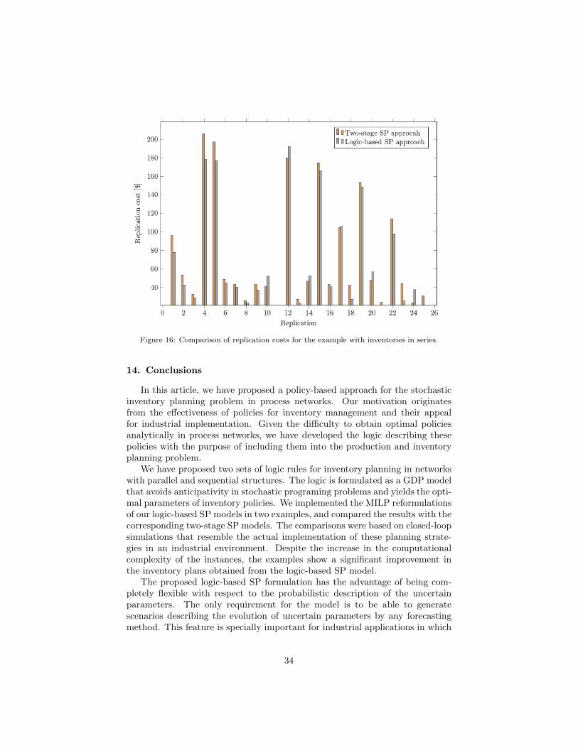
Figure 16: Comparison of replication costs for the example with inventories in series.

14. Conclusions

In this article, we have proposed a policy-based approach for the stochasticinventory planning problem in process networks. Our motivation originatesfrom the effectiveness of policies for inventory management and their appealfor industrial implementation. Given the difficulty to obtain optimal policiesanalytically in process networks, we have developed the logic describing thesepolicies with the purpose of including them into the production and inventoryplanning problem.

We have proposed two sets of logic rules for inventory planning in networkswith parallel and sequential structures. The logic is formulated as a GDP modelthat avoids anticipativity in stochastic programing problems and yields the opti-mal parameters of inventory policies. We implemented the MILP reformulationsof our logic-based SP models in two examples, and compared the results with thecorresponding two-stage SP models. The comparisons were based on closed-loopsimulations that resemble the actual implementation of these planning strate-gies in an industrial environment. Despite the increase in the computationalcomplexity of the instances, the examples show a significant improvement inthe inventory plans obtained from the logic-based SP model.

The proposed logic-based SP formulation has the advantage of being com-pletely flexible with respect to the probabilistic description of the uncertainparameters. The only requirement for the model is to be able to generatescenarios describing the evolution of uncertain parameters by any forecastingmethod. This feature is specially important for industrial applications in which

34

correlation and autocorrelation of the uncertain parameters is very common,and allows using historical data in the inventory planning model.

The logic developed for inventory planning in process networks with paral-lel and sequential structures can be extended to address networks of arbitrarytopology with complex uncertainty models. There is an extraordinary potentialfor inventory optimization in these networks because their complexity concealsthe most effective planning strategies. This contribution offers a novel approachfor a very challenging problem particular to the process industry.

References

[1] S. Bose and J. F. Pekny. A model predictive framework for planning and schedul-ing problems: a case study of consumer goods supply chain. Computers & Chem-ical Engineering, 24:329–335, 2000.

[2] Yunfei Chu, Fengqi You, John M. Wassick, and Anshul Agarwal. Integrated plan-ning and scheduling under production uncertainties: Bi-level model formulationand hybrid solution method. Computers & Chemical Engineering, 72:255 – 272,2015.

[3] Yunfei Chu, Fengqi You, John M Wassick, and Anshul Agarwal. Simulation-basedoptimization framework for multi-echelon inventory systems under uncertainty.Computers & Chemical Engineering, 73:1–16, 2015.

[4] A. J. Clark and H. Scarf. Optimal policies for a multi-echelon inventory problem.Management Science, 50:1782–1790, 2004.

[5] E.B. Diks and A.G. de Kok. Optimal control of a divergent multi-echelon inven-tory system. European Journal of Operational Research, 111:75–97, 1998.

[6] G. Eppen and L. Schrage. Multi-Level Production/Inventory Control Systems:Theory and Practice, chapter Centralized ordering policies in a multi-warehousesystem with lead times and random demand, page 5167. North-Holland, Amster-dam, The Netherlands, 1981.

[7] Laureano F. Escudero, Araceli Garın, Marıa Merino, and Gloria Perez. The valueof the stochastic solution in multistage problems. 15:48–64, 2007.

[8] M. Ettl, G. E. Feigin, G. Y. Lin, and D. D. Yao. A supply network model withbase-stock control and service requirements. Operations Research, 48:216–232,2000.

[9] A. Federgruen and P. Zipkin. An inventory model with limited production ca-pacity and uncertain demands i. the average-cost criterion. Mathematics of Op-erations Research, 11:193–207, 1986.

[10] A. Federgruen and P. Zipkin. An inventory model with limited production ca-pacity and uncertain demands ii. the discounted-cost criterion. Mathematics ofOperations Research, 11:208–215, 1986.

35

[11] Awi Federgruen and Paul Zipkin. Allocation policies and cost approximations formultilocation inventory systems. Naval Research Logistics Quarterly, 31:97–129,1984.

[12] Awi Federgruen and Paul Zipkin. Computational issues in an infinite-horizon,multiechelon inventory model. Operations Research, 32:818–836, 1984.

[13] P. Glasserman and S. Tayur. Sensitivity analysis for base-stock levels in multi-echelon production-inventory systems. Management Science, 41:263–281, 1995.

[14] S. C. Graves and S. P. Willems. Optimizing strategic safety stock placement insupply chains. Manufacturing & Service Operations Management, 2:68–83, 2000.

[15] Stephen C. Graves. A multiechelon inventory model with fixed replenishmentintervals. Management Science, 42:1–18, 1996.

[16] I. E. Grossmann. Enterprise-wide optimization: A new frontier in process systemsengineering. Aiche Journal, 51:1846–1857, 2005.

[17] F. W. Harris. How many parts to make at once. Operations Research, 38:947–950,1990.

[18] Marianthi G. Ierapetritou and Efstratios N. Pistikopoulos. Batch plant designand operations under uncertainty. Industrial & Engineering Chemistry Research,35:772–787, 1996.

[19] Karl Inderfurth. Safety stock optimization in multi-stage inventory systems. In-ternational Journal of Production Economics, 24:103–113, 1991.

[20] Karl Inderfurth and Stefan Minner. Safety stocks in multi-stage inventory systemsunder different service measures. European Journal of Operational Research, 106:57–73, 1998.

[21] James R. Jackson. Networks of waiting lines. Operations Research, 5:518–521,1957.

[22] June Young Jung, Gary Blau, Joseph F. Pekny, Gintaras V. Reklaitis, and DavidEversdyk. Integrated safety stock management for multi-stage supply chains un-der production capacity constraints. Computers & Chemical Engineering, 32:2570–2581, 2008.

[23] J.Y. Jung, G. Blau, J.F. Pekny, Reklaitis G.V., and D. Eversdyk. A simula-tion based optimization approach to supply chain management under demanduncertainty. Computers and Chemical Engineering, 28:20872106, 2004.

[24] I. A. Karimi and G. V. Reklaitis. Optimal selection of intermediate storage tankcapacity in a periodic batch/semicontinuous process. AIChE Journal, 29:588–596,1983.

[25] G. E. Kimball. General principles of inventory control. Journal of Manufacturingand Operations Management, 1:119–130, 1988. Original from 1955.

[26] A.J. Kleywegt, A. Shapiro, and T. Homem-de Mello. The sample average approx-imation method for stochastic discrete optimization. SIAM J. on Optimization,12:479–502, 2002.

36

[27] W. Klibi and A. Martel. Modeling approaches for the design of resilient supplynetworks under disruptions. International Journal of Production Economics, 135:882–898, 2012.

[28] Daniel Kuhn, Wolfram Wiesemann, and Angelos Georghiou. Primal and duallinear decision rules in stochastic and robust optimization. Mathematical Pro-gramming, 130:177–209, 2011.

[29] Hau L. Lee and Corey Billington. Material management in decentralized supplychains. Operations Research, 41(5):835–847, 1993.

[30] Yong-Joo Lee and Paul Zipkin. Tandem queues with planned inventories. Oper-ations Research, 40:936–947, 1992.

[31] E. Perea-Lopez, I. E. Grossmann, and T. Ydstie, B. E.and Tahmassebi. Dynamicmodeling and decentralized control of supply chains. Industrial & EngineeringChemistry Research, 40:3369–3383, 2001.

[32] Edgar Perea-Lopez, B.Erik Ydstie, and Ignacio E. Grossmann. A model pre-dictive control strategy for supply chain optimization. Computers & ChemicalEngineering, 27:1201–1218, 2003.

[33] S. B. Petkov and C. D. Maranas. Design of single-product campaign batch plantsunder demand uncertainty. AIChE Journal, 44:896–911, 1998.

[34] J.B. Rawlings, D. Angeli, and C.N. Bates. Fundamentals of economic modelpredictive control. In Decision and Control (CDC), 2012 IEEE 51st AnnualConference on, pages 3851–3861, 2012.

[35] Stephen M. Robinson. Analysis of sample-path optimization. Mathematics ofOperations Research, 21:513–528, 1996.

[36] Kaj Rosling. Optimal inventory policies for assembly systems under randomdemands. Operations Research, 37:565–579, 1989.

[37] T. Santoso, S. Ahmed, M. Goetschalckx, and A. Shapiro. A stochastic program-ming approach for supply chain network design under uncertainty. EuropeanJournal of Operational Research, 167:96–115, 2005.

[38] P. Schutz, A. Tomasgard, and S. Ahmed. Supply chain design under uncertaintyusing sample average approximation and dual decomposition. European Journalof Operational Research, 199:409–419, 2009.

[39] Nilay Shah and Constantinos C. Pantelides. Design of multipurpose batch plantswith uncertain production requirements. Industrial & Engineering ChemistryResearch, 31:1325–1337, 1992.

[40] K. H. Shang and J-S. Song. Newsvendor bounds and heuristic for optimal policiesin serial supply chains. Management Science, 49:618–638, 2003.

[41] A. Shapiro and T. Homem-de Mello. A simulation-based approach to two-stagestochastic programming with recourse. Mathematical Programming, 81:301–325,1998.

37

[42] Kenneth F. Jr. Simpson. In-process inventories. Operations Research, 6(6):863–873, 1958.

[43] D.A. Straub and I.E. Grossmann. Integrated stochastic metric of flexibility forsystems with discrete state and continuous parameter uncertainties. Computers& Chemical Engineering, 14:967–985, 1990.

[44] S. Subrahmanyam, J. F. Pekny, and G. V. Reklaitis. Design of batch chemicalplants under market uncertainty. Industrial & Engineering Chemistry Research,33:2688–2701, 1994.

[45] Kaushik Subramanian, Christos T. Maravelias, and James B. Rawlings. A state-space model for chemical production scheduling. Computers & Chemical Engi-neering, 47:97 – 110, 2012.

[46] Kaushik Subramanian, James B. Rawlings, Christos T. Maravelias, Jesus Flores-Cerrillo, and Lawrence Megan. Integration of control theory and scheduling meth-ods for supply chain management. Computers & Chemical Engineering, 51:4–20,2013.

[47] Sridhar R. Tayur. Computing the optimal policy for capacitated inventory models.Communications in Statistics. Stochastic Models, 9:585–598, 1993.

[48] Sebastian Terrazas-Moreno, Ignacio E. Grossmann, John M. Wassick, and Scott J.Bury. Optimal design of reliable integrated chemical production sites. Computers& Chemical Engineering, 34:1919–1936, 2010.

[49] Sebastian Terrazas-Moreno, Ignacio E. Grossmann, John M. Wassick, Scott J.Bury, and Naoko Akiya. An efficient method for optimal design of large-scaleintegrated chemical production sites with endogenous uncertainty. Computers &Chemical Engineering, 37:89–103, 2012.

[50] I. Thomas, W. Abriatis, and C. Savage. Manufacturing and Trade: Inventoriesand Sales - December 2013. U.S. Department of Commerce, 2013.

[51] P. Tsiakis, N. Shah, and C. C. Pantelides. Design of multi-echelon supply chainnetworks under demand uncertainty. Industrial & Engineering Chemistry Re-search, 40:3585–3604, 2001.

[52] G.J. van Houtum and W.H.M. Zijm. Computational procedures for stochas-tic multi-echelon production systems. International Journal of Production Eco-nomics, 23:223 – 237, 1991.

[53] H. S. Wellons and G. V. Reklaitis. The design of multiproduct batch plantsunder uncertainty with staged expansion. Computers & Chemical Engineering,13:115–126, 1989.

[54] R. Wilson. 24th Annual State of Logistic Report. Counsil of Supply Chain Man-agement Professionals, 2013.

[55] F. You, J. M. Wassick, and I. E. Grossmann. Risk management for a global supplychain planning under uncertainty: Models and algorithms. AIChE Journal, 55:931–946, 2009.

38

[56] Fengqi You and Ignacio E. Grossmann. Integrated multi-echelon supply chain de-sign with inventories under uncertainty: Minlp models, computational strategies.AIChE Journal, 56:419–440, 2010.

[57] Fengqi You and Ignacio E. Grossmann. Stochastic inventory management for tac-tical process planning under uncertainties: Minlp models and algorithms. AIChEJournal, 57:1250–1277, 2011.

[58] Dajun Yue and Fengqi You. Planning and scheduling of flexible process networksunder uncertainty with stochastic inventory: Minlp models and algorithm. AIChEJournal, 59:1511–1532, 2013.

39