Optimizing Daily Agent Schedulingin a Multiskill Call Center

Athanassios N. AvramidisSchool of Mathematics, University of Southampton

Highfield, Southampton, SO17 1BJ, UNITED KINGDOM

Wyean ChanDepartement d’informatique et de recherche operationnelle

Universite de Montreal, C.P. 6128, Succ. Centre-VilleMontreal (Quebec), H3C 3J7, CANADA

Michel GendreauDepartement d’informatique et de recherche operationnelle and CIRRELT

Universite de Montreal, C.P. 6128, Succ. Centre-VilleMontreal (Quebec), H3C 3J7, CANADA

Pierre L’EcuyerDepartement d’informatique et de recherche operationnelle, CIRRELT and GERAD

Universite de Montreal, C.P. 6128, Succ. Centre-VilleMontreal (Quebec), H3C 3J7, CANADA

Ornella PisacaneDipartimento di Elettronica Informatica e Sistemistica

Universita della Calabria, Via P. Bucci, 41CArcavacata di Rende (CS), ITALY

January 19, 2009

Abstract

We examine and compare simulation-based algorithms for solving the agent scheduling problem in amultiskill call center. This problem consists in minimizing the total costs of agents under constraintson the expected service level per call type, per period, and aggregated. We propose a solutionapproach that combines simulation with integer or linear programming, with cut generation. In ournumerical experiments with realistic problem instances, this approach performs better than all other

1

methods proposed previously for this problem. We also show that the two-step approach, which isthe standard method for solving this problem, sometimes yield solutions that are highly suboptimaland inferior to those obtained by our proposed method.

1 Introduction

The telephone call center industry employs millions of people around the world and is fast growing.In the United States, for example, customer service representatives held 2.1 million jobs in 2004,and employment in this job category is expected to increase faster than average at least through 2014(Bureau of Labor Statistics 2007). A few percent saving in workforce salaries easily means severalmillion dollars.

Call centers often handle several types of calls distinguished by the required skills for deliveringservice. Training all agents to handle all call types is not cost-effective. Each agent has a selectednumber of skills and the agents are distinguished by the set of call types they can handle (also calledtheir skill set). When such skill constraints exist, we speak of a multiskill call center. Skill-based

routing (SBR), or simply routing, refers to the rules that control the call-to-agent and agent-to-callassignments. Most modern call centers perform skill-based routing (Koole and Mandelbaum 2002,Gans et al. 2003).

In a typical call center, inbound calls arrive at random according to some complicated stochasticprocesses, call durations are also random, waiting calls may abandon after a random patience time,some agents may fail to show up to work for any reason, and so on. Based on forecasts of callvolumes, call center managers must decide (among other things) how many agents of each type (i.e.,skill set) to have in the center at each time of the day, must construct working schedules for theavailable agents, and must decide on the call routing rules. These decisions are made under a highlevel of uncertainty. The goal is typically to provide the required quality of service at minimal cost.

The most common measure of quality of service is the service level (SL), defined as the long-term fraction of calls whose time in queue is no larger than a given threshold. Frequently, multiplemeasures of SL are of interest: for a given time period of the day, for a given call type, for a givencombination of call type and period, aggregated over the whole day and all call types, and so on. Forcertain call centers that provide public services, SL constraints are imposed by external authorities,and violations may result in stiff penalties (CRTC 2000).

In this paper, we assume that we have a detailed stochastic model of the dynamics of the callcenter for one day of operation. This model specifies the stochastic processes for the call arrivals(these processes are usually non-stationary and doubly stochastic), the distributions of service timesand patience times for calls, the call routing rules, the periods of unavailability of agents betweencalls (e.g., to fill out forms, or to go to the restroom, etc.), and so forth. We formulate a stochasticoptimization problem where the objective is to minimize the total cost of agents, under various SL

2

constraints. This could be used in long-term planning, to decide how many agents to hire and forwhat skills to train them, or for short-term planning, to decide which agents to call for work on agiven day and what would be their work schedule. The problem is difficult because for any givenfixed staffing of agents (the staffing determines how many agents of each type are available in eachtime period), no reliable formulas or quick numerical algorithms are available to estimate the SL;it can be estimated accurately only by long (stochastic) simulations. Scheduling problems are ingeneral NP-hard, even in deterministic settings where each solution can be evaluated quickly andexactly. When this evaluation requires costly and noisy simulations, as is the case here, solving theproblem exactly is even more difficult and we must settle with methods that are partly heuristic.

Staffing in the single-skill case (i.e., single call type and single agent type) has received muchattention in the call center literature. Typically, the workload varies considerably during the day(Gans et al. 2003, Avramidis et al. 2004, Brown et al. 2005), and the planned staffing can changeonly at a few discrete points in time (e.g., at the half hours). It is common to divide the day intoseveral periods during which the staffing is held constant and the arrival rate does not vary much.If the system can be assumed to reach steady-state quickly (relative to the length of the periods),then steady-state queueing models are likely to provide a reasonably good staffing recommendationfor each period. For instance, in the presence of abandonments, one can use an Erlang-A formulato determine the minimal number of agents for the required SL in each period (Gans et al. 2003).When that number is large, it is often approximated by the square root safety staffing formula, basedon the Halfin-Whitt heavy-traffic regime, and which says roughly that the capacity of the systemshould be equal to the workload plus some safety staffing which is proportional to the square root ofthe workload (Halfin and Whitt 1981, Gans et al. 2003). This commonly used heuristic, known asthe stationary independent period by period (SIPP) approach, often fails to meet target SL becauseit neglects the non-stationarity (Green et al. 2003). Non-stationary versions of these approximationshave also been developed, still for the single-skill case (Jennings et al. 1996, Green et al. 2003).

Scheduling problems are often solved in two separate steps (Mehrotra 1997): After an appropriatestaffing has been determined for each period in the first step, a minimum-cost set of shifts thatcovers this staffing requirement can be computed in the second step by solving a linear integerprogram. However, the constraints on admissible working shifts often force the second step solutionto overstaff in some of the periods. This drawback of the two-step approach has been pointed outby several authors, who also proposed alternatives (Keith 1979, Thompson 1997, Henderson andMason 1998, Ingolfsson et al. 2003, Atlason et al. 2004). For example, the SL constraint is oftenonly for the time-aggregated (average) SL over the entire day; in that case, one may often obtaina lower-cost scheduling solution by reducing the minimal staffing in one period and increasing itin another period. Atlason et al. (2004) developed a simulation-based methodology to optimizeagents’ scheduling in the presence of uncertainty and general SL constraints, based on simulationand cutting-plane ideas. Linear inequalities (cuts) are added to an integer program until its optimal

3

solution satisfies the required SL constraints. The SL and the cuts are estimated by simulation.In the multiskill case, the staffing and scheduling problems are more challenging, because the

workload can be covered by several possible combinations of skill sets, and the routing rules alsohave a strong impact on the performance. Staffing a single period in steady-state is already difficult;the Erlang formulas and their approximations (for the SL) no longer apply. Simulation seems to bethe only reliable tool to estimate the SL. Cezik and L’Ecuyer adapt the simulation-based method-ology of Atlason et al. (2004) to the optimal staffing of a multiskill call center for a single period.They point out difficulties that arise with this methodology and develop heuristics to handle them.Avramidis et al. (2006) solve the same problem by using neighborhood search methods combinedwith an analytical approximation of SLs, with local improvement via simulation at the end. Pot et al.(2007) impose a constraint only on the aggregate SL (across all call types); they solve Lagrangeanrelaxations using search methods and analytical approximations.

Some authors have studied the special case where there are only two call types, and some havedeveloped queueing approximations for the case of two call types, via Markov chains and undersimplifying assumptions; see Stolletz and Helber (2004) for example. But here we are thinking of20 to 50 call types or more, which is common in modern call centers, and for which computationvia these types of Markov chain models is clearly impractical.

For the multiskill scheduling problem, Bhulai et al. (2007) propose a two-step approach in whichthe first step determines a staffing of each agent type for each period, and the second step computesa schedule by solving an IP in which this staffing is the right-hand side of key constraints. A keyfeature of the IP model is that the staff-coverage constraints allow downgrading an agent into anyalternative agent type with smaller skill set, temporarily and separately for each period. Bhulai et al.(2007) recognize that their two-step approach is generally suboptimal and they illustrate this byexamples.

In this paper, we propose a simulation-based algorithm for solving the multiskill schedulingproblem, and compare it to the approach of Bhulai et al. (2007). This algorithm extends the methodof Cezik and L’Ecuyer, which solves a single-period staffing problem. In contrast to the two-stepapproach, our method optimizes the staffing and the scheduling simultaneously. Our numericalexperiments show that our algorithm provides approximate solutions to large-scale realistic probleminstances in reasonable time (a few hours). These solutions are typically better, sometimes by alarge margin (depending on the problem), than the best solutions from the two-step approach. Weare aware of no competitive faster method.

The remainder of this paper is organized as follows. In section 2, we formally define the problemat hand and provide a mathematical programming formulation. The new algorithm is described in3. We report computational results on several test instances in section 4. The conclusion follows.A preliminary version of this paper was presented at the 2007 Industrial Simulation Conference(Avramidis et al. 2007a).

4

2 Model Formulation

We now provide definitions of the multiskill staffing and scheduling problems. We assume that wehave a stochastic model of the call center, under which the mathematical expectations used beloware well defined, and that we can simulate the dynamics of the center under this model. Our problemformulations here do not depend on the details of this model.

There are K call types, labeled from 1 to K, and I agent types, labeled from 1 to I. Agent type i

has the skill set Si ⊆ {1, . . . ,K}. The day is divided into P periods of given length, labeled from 1 toP. The staffing vector is y = (y1,1, . . . ,y1,P, . . . ,yI,1, . . . ,yI,P)t where yi,p is the number of agents oftype i available in period p. Given y, the service level (SL) in period p for type-k calls is defined as

gk,p(y) = E[Cg,k,p]/E[Ck,p +Ak,p],

where E denotes the mathematical expectation, Ck,p is the number of type-k calls that arrive inperiod p and eventually get served, Cg,k,p is the number of those calls that get served after waitingat most τk,p (a constant called the acceptable waiting time), and Ak,p is the number of those callsthat abandon after waiting at least τk,p. Aggregate SLs, per call type, per period, and globally, aredefined analogously. Given acceptable waiting times τp, τk, and τ , the aggregate SLs are denoted bygp(y), gk(y) and g(y) for period p, call type k, and overall, respectively.

A shift is a time pattern that specifies the periods in which an agent is available to handle calls. Inpractice, it is characterized by its start period (the period in which the agent starts working), break

periods (the periods when the agent stops working), and end period (the period when the agentfinishes his/her workday). In general, agents have several breaks of different duration; for instance,morning and afternoon coffee breaks, as well as a longer lunch break.

Let {1, . . . ,Q} be the set of all admissible shifts. To simplify the exposition, we assume that thisset is the same for all agent types; this assumption could easily be relaxed if needed, by introducingspecific shift sets for each agent type. The admissible shifts are specified via a P×Q matrix A0

whose element (p,q) is ap,q = 1 if an agent with shift q works in period p, and 0 otherwise. Avector x = (x1,1, . . . ,x1,Q, . . . ,xI,1, . . . ,xI,Q)t, where xi,q is the number of agents of type i workingshift q, is a schedule. The cost vector is c = (c1,1, . . . ,c1,Q, . . . ,cI,1, . . . ,cI,Q)t, where ci,q is the costof an agent of type i with shift q. To any given shift vector x, there corresponds the staffing vectory = Ax, where A is a block-diagonal matrix with I identical blocks A0, if we assume that each agentof type i works as a type-i agent for his/her entire shift.

However, following Bhulai et al. (2007), we also allow an agent of type i to be temporarilydowngraded to an agent with smaller skill set, i.e., of type ip where Sip ⊂ Si, in any time period p

of his/her shift. Define S +i = { j : S j ⊃ Si∧ 6 ∃m : S j ⊃ Sm ⊃ Si} (S +

i is thus the set of agent typeswhose skill set is a minimum strict superset of the skill set of agent type i) and S −

i = { j : S j ⊂ Si∧ 6∃m : S j ⊂ Sm ⊂ Si} (S −

i is thus the set of agent types whose skill set is a maximum strict subsetof skill set of agent type i). To illustrate, consider a call centre with K = 3 call types, I = 4 agent

5

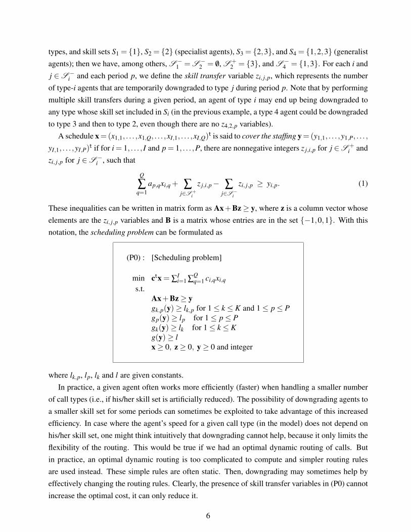
types, and skill sets S1 = {1}, S2 = {2} (specialist agents), S3 = {2,3}, and S4 = {1,2,3} (generalistagents); then we have, among others, S −

1 = S −2 = /0, S +

2 = {3}, and S −4 = {1,3}. For each i and

j ∈S −i and each period p, we define the skill transfer variable zi, j,p, which represents the number

of type-i agents that are temporarily downgraded to type j during period p. Note that by performingmultiple skill transfers during a given period, an agent of type i may end up being downgraded toany type whose skill set included in Si (in the previous example, a type 4 agent could be downgradedto type 3 and then to type 2, even though there are no z4,2,p variables).

A schedule x =(x1,1, . . . ,x1,Q, . . . ,xI,1, . . . ,xI,Q)t is said to cover the staffing y =(y1,1, . . . ,y1,P, . . . ,

yI,1, . . . ,yI,P)t if for i = 1, . . . , I and p = 1, . . . ,P, there are nonnegative integers z j,i,p for j ∈S +i and

zi, j,p for j ∈S −i , such that

Q

∑q=1

ap,qxi,q + ∑j∈S +

i

z j,i,p− ∑j∈S −

i

zi, j,p ≥ yi,p. (1)

These inequalities can be written in matrix form as Ax+Bz≥ y, where z is a column vector whoseelements are the zi, j,p variables and B is a matrix whose entries are in the set {−1,0,1}. With thisnotation, the scheduling problem can be formulated as

(P0) : [Scheduling problem]

min ctx = ∑Ii=1 ∑

Qq=1 ci,qxi,q

s.t.Ax+Bz≥ ygk,p(y)≥ lk,p for 1≤ k ≤ K and 1≤ p≤ Pgp(y)≥ lp for 1≤ p≤ Pgk(y)≥ lk for 1≤ k ≤ Kg(y)≥ lx≥ 0, z≥ 0, y≥ 0 and integer

where lk,p, lp, lk and l are given constants.In practice, a given agent often works more efficiently (faster) when handling a smaller number

of call types (i.e., if his/her skill set is artificially reduced). The possibility of downgrading agents toa smaller skill set for some periods can sometimes be exploited to take advantage of this increasedefficiency. In case where the agent’s speed for a given call type (in the model) does not depend onhis/her skill set, one might think intuitively that downgrading cannot help, because it only limits theflexibility of the routing. This would be true if we had an optimal dynamic routing of calls. Butin practice, an optimal dynamic routing is too complicated to compute and simpler routing rulesare used instead. These simple rules are often static. Then, downgrading may sometimes help byeffectively changing the routing rules. Clearly, the presence of skill transfer variables in (P0) cannotincrease the optimal cost, it can only reduce it.

6

Suppose we consider a single period, say period p, and we replace gk,p(y) and gp(y) by approx-imations that depend on the staffing of period p only, say gk,p(y1,p, . . . ,yI,p) and gp(y1,p, . . . ,yI,p),respectively. If all system parameters are assumed constant over period p, then natural approxima-tions are obtained by assuming that the system is in steady-state over this period. The single-periodmultiskill staffing problems can then be written as

(P1) : [Staffing problem]

min ∑Ii=1 ciyi

s.t.gk(y1, . . . ,yI)≥ lk for 1≤ k ≤ Kg(y1, . . . ,yI)≥ lyi ≥ 0 and integer for all i

where ci is the cost of agent type i (for a single period), and the period index was dropped through-out. Simulation-based solution methods for this problem are proposed in Cezik and L’Ecuyer andAvramidis et al. (2006). Pot et al. (2007) address a restricted version of it, with a single constrainton the aggregate SL over the period (i.e., they assume lk = 0 for all k).

In the approach of Bhulai et al. (2007), the first step is to determine an appropriate staffing,y = (y1,1, . . . , y1,P, . . . , yI,1, . . . , yI,P)t. For this, they look at each period p in isolation and solve aversion of (P1) with a single constraint on the aggregate SL; this gives y1,p, . . . , yI,p for each p. Intheir second step, they find a schedule that covers this staffing by solving:

(P2) : [Two-stage approach]

min ctxs.t.

Ax+Bz≥ yx≥ 0,z≥ 0 and integer

The presence of skill-transfer variables generally reduces the optimal cost in (P2) by addingflexibility, compared with the case where no downgrading is allowed. However, there sometimesremains a significant gap between the optimal solution of (P0) and the best solution found for thesame problem by the two-step approach. The following simplified example illustrates this.

Example 1 Let K = I = P = 3, and Q = 1. The single type of shift covers the three periods. Theskill sets are S1 = {1,2}, S2 = {1,3}, and S3 = {2,3}. All agents have the same shift and the samecost. Suppose that the total arrival process is stationary Poisson with mean 100 per minute. Thisincoming load is equally distributed between call types {1,2} in period 1, {1,3} in period 2, {2,3}

7

in period 3. Any agent can be downgraded to a specialist that can handle a single call type (thatbelongs to his skill set), in any period. In the presence of such specialists, an incoming call goesfirst to its corresponding specialist if there is one available, otherwise it goes to a generalist thatcan handle another call type as well. When the agent becomes available, he serves the call that haswaited the longest among those in the queue (if any). The service times are exponential with mean1 per minute, there are no abandonments, and the SL constraints specify that 80% of all calls mustbe served within 20 seconds, in each time period, on average over an infinite number of days.

If we assume that the system operates in steady-state in period 1, then the optimal staffing for thatperiod is 104 agents of type 1. Since all agents can serve all calls, we have in this case an M/M/s

queue with s = 104, and the global SL is 83.4%, as can be computed by the well-known Erlang-Cformula (Gans et al. 2003). By symmetry, the optimal staffing solutions for the other periods areobviously the same: 104 agents of type 2 in period 2 and 104 agents of type 3 in period 3. Then, thetwo-step approach gives a solution to (P2) with 104 agents of each type, for a total of 312 agents.

Solving (P0) directly instead (e.g., using the simulation-based algorithm described in the nextsection), assuming again (as an approximation) that the system is in steady-state in each of the threeperiods, we find a feasible solution with 35 agents of type 1, 35 agents of type 2, and 34 agents oftype 3, for a total of 104 agents. With this solution, during period 1, the agents of types 2 and 3 aredowngraded to specialists who handle only call types 1 and 2, respectively, and the agents of type 1act as generalists. A similar arrangement applies to the other periods, mutatis mutandis. Note thatthis solution of (P0) remains valid even if we remove the skill transfer variables from the formulationof (P0), because the sets S−i and S+

i are all empty, if we assume that the routing rules do not change;i.e., if calls are always routed first to agents that can handle only this call type among the calls thatcan arrive during the current period.

Suppose now that we add the additional skill sets S4 = {1}, S5 = {2}, S6 = {3}, and that thesenew specialists cost 6 each, whereas the agents with two skills cost 7. In this case it becomesattractive to use specialists to handle a large fraction of the load, because they are less expensive,and to keep a few generalists in each period to obtain a “resource sharing” effect. It turns out thatan optimal staffing solution for period 1 is 2 generalists (type 1) and 52 specialists of each of thetypes 4 and 5. An analogous solution holds for each period. With these numbers, if downgradingis not possible, the two-step approach gives a solution with 6 generalists (2 of each type) and 156specialists (52 of each type), for a total cost of 978. If downgrading is allowed, then the two-stepapproach finds the following much better solution: 2 agents of type 1 and 52 of each of the types 2and 3, for a total cost of 742. The skill transfer works in this way. In period 1: 52 agents of type2 are downgraded to specialists of type 4 and 52 of type 3 to specialists of type 5. In period 2: 2agents of type 1 are downgraded to agents of type 4, 52 of type 2 to type 6 and 50 of type 3 to type4. In period 3: 2 agents of type 1 are downgraded to agents of type 5, 50 of type 2 to type 5 and 52of type 3 to type 6. If we solve (P0) directly with these additional skill sets, we get the same solution

8

as without them; i.e., 104 agents with two skills each, for a total cost of 728. This is again betterthan with the two-step approach, but the gap is much smaller than what we had with only three skillsets.

Example 2 In the previous example, if all the load was from a single call type, there would be asingle agent type and the two-step approach would provide exactly the same solution as the optimalsolution of (P0). The example illustrates a suboptimality gap due to a variation in the type of load.

Another potential source of suboptimality (this one can occur even in the case of a single calltype) is the time variation of the total load from period to period. If there is only a global SLconstraint over the entire day, then the optimal solution may allow a lower SL during one (or more)peak period(s) and recover an acceptable global SL by catching up in the other periods. To accountfor this, Bhulai et al. (2007), Section 5.4, propose a heuristic based on the solution obtained by theirbasic two-step approach. Although this appears to work well in their examples, the effectiveness ofthis heuristic for general problems is not clear.

Yet another type of limitation that can significantly increase the total cost is the restriction onthe set of available shifts. Suppose for example that there is a single call type, that the day has 10periods, and that all shifts must cover 8 periods, with 7 periods of work and a single period of lunchbreak after 3 or 4 periods of work. Thus a shift can start in period 1, 2, or 3, and there are six shifttypes in total. Suppose we need 100 agents available in each period. For this we clearly need 200agents, each one working for 7 periods, for a total of 1400 agent-periods. If there were no constraintson the duration and shape of shifts, on the other hand, then 1000 agent-periods would suffice.

3 Optimization by Simulation and Cutting Planes

We now describe the proposed simulation-based optimization algorithm. The general idea is toreplace the problem (P0) by a sample version of it, (SP0n), and then replace the nonlinear SL con-straints by a small set of linear constraints, in a way that the optimal solution of the resulting relaxed

sample problem is close to that of (P0). The relaxed sample problem is solved by linear or integerprogramming.

We first describe how the relaxation works when applied directly to (P0); it works the same waywhen applied to the sample problem. Consider a version of (P0) in which the SL constraints havebeen replaced by a small set of linear constraints that do not cut out the optimal solution. Let y bethe optimal solution of this (current) relaxed problem. If y satisfies all SL constraints of (P0), thenit is an optimal solution of (P0) and we are done. Otherwise, take a violated constraint of (P0), sayg(y) < l, suppose that g is (jointly) concave in y for y≥ y, and that q is a subgradient of g at y. Then

g(y)≤ g(y)+ qt(y− y)

9

for all y≥ y. We want g(y)≥ l, so we must have

l ≤ g(y)≤ g(y)+ qt(y− y),

i.e.,qty≥ qty+ l−g(y). (2)

Adding this linear cut inequality to the constraints removes y from the current set of feasible solu-tions of the relaxed problem without removing any feasible solution of (P0). On the other hand, incase q is not really a subgradient (which may happens in practice), then we may cut out feasiblesolutions of (P0), including the optimal one. We will return to this.

Since we cannot evaluate the functions g exactly, we replace them by a sample average over n

independent days, obtained by simulation. Let ω represent the sequence of independent uniformrandom numbers that drives the simulation for those n days. When simulating the call center fordifferent values of y, we assume that the same uniform random numbers are used for the samepurpose for all values of y, for each day. That is, we use the same ω for all y. Proper synchronizationof these common random numbers is implemented by using a random number package with multiplestreams and substreams (Law and Kelton 2000, L’Ecuyer et al. 2002, L’Ecuyer 2004).

The empirical SL over these n simulated days is a function of the staffing y and of ω . We denote itby gn,k,p(y,ω) for call type k in period p; gn,p(y,ω) aggregated over period p; gn,k(y,ω) aggregatedfor call type k; and gn(y,ω) aggregated overall. For a fixed ω , these are all deterministic functionsof y. Instead of solving directly (P0), we solve its sample-average approximation (SP0n) obtainedby replacing the functions g in (P0) by their sample counterparts g (here, g stands for any of theempirical SL functions, and similarly for g).

We know that gn,k,p(y) converges to gk,p(y) with probability 1 for each (k, p) and each y whenn → ∞. In this sense, (SP0n) converges to (P0) when n → ∞. Suppose that we eliminate a priori allbut a finite number of solutions for (P0). This can easily be achieved by eliminating all solutions forwhich the total number of agents is unreasonably large. Let Y ∗ be the set of optimal solutions of(P0) and suppose that no SL constraint is satisfied exactly for these solutions. Let Y ∗

n be the set ofoptimal solutions of (SP0n). Then, the following theorem implies that for n large enough, an optimalsolution to the sample problem is also optimal for the original problem. It can be proved by a directadaptation of the results of Vogel (1994) and Atlason et al. (2004); see also Cezik and L’Ecuyer.

Theorem 1 With probability 1, there is an integer N0 < ∞ such that for all n ≥ N0, Y ∗n = Y ∗.

Moreover, suppose that the service-level estimators satisfy the standard large-deviation principle (a

mild assumption): For every ε > 0, there are positive integers N0 and κ such that for all n≥ N0 and

y ∈ Y , P(|gn,k,p(y,ω)−gk,p(y)|> ε

)≤ e−nκ for all k, p, and for the aggregate service-levels as

well. Then, there are positive real numbers α and β such that for all n,

P[Y ∗n = Y ∗]≥ 1−αe−βn.

10

We solve (SP0n) by the cutting plane method described earlier, with the functions g replacedby their empirical counterparts. The major practical difficulty is to obtain the subgradients q. Infact, the functions g in the empirical problem (computed by simulation) are not necessarily concavefor finite n, even in the areas where the functions g of (P0) are concave. To obtain a (tentative)subgradient q of a function g at y, we use forward finite differences as follows. For j = 1, . . . , IP,we choose an integer d j ≥ 0, we compute the function g at y and at y+d je j for j = 1, . . . , IP, wheree j is the jth unit vector, and we define q as the IP-dimensional vector whose jth component is

q j = [g(y+d je j)− g(y)]/d j. (3)

In our experiments, we used the same heuristic as in Cezik and L’Ecuyer to select the d j’s: Wetook d j = 3 when the SL corresponding to the considered cut was less than 0.5, d j = 2 when it wasbetween 0.5 and 0.65, and d j = 1 when it was greater than 0.65. When we need a subgradient for aperiod-specific empirical SL (gp or gk,p), the finite difference is formed only for those components ofy corresponding to the given period; the other elements of q are set to zero. This heuristic introducesinaccuracies, because gp and gk,p depend in general on the staffing of all periods up to p or evenp+1, but it reduces the work significantly.

Computing q via (3) requires IP + 1 simulations of n days each. This is by far the most time-consuming part of the algorithm. Even for medium-size problems, these simulations can easilyrequire an excessive amount of time. For this reason, we use yet another important short-cut: Wegenerally use a smaller value of n for estimating the subgradients than for checking feasibility. (Thelatter requires a single n-day simulation experiment.) That is, we compute each g(y + d je j) in (3)using n0 < n days of simulation, instead of n days. In most of our experiments (including thosereported in this paper), we have used n0 ≈ n/10.

With all these approximations and the simulation noise, we recognize that the vector q thusobtained is only a heuristic guess for a subgradient. It may fail to be a subgradient. In that casethe cut (2) may remove feasible staffing solutions including the optimal one, and this may lead ouralgorithm to a suboptimal schedule; Atlason et al. (2004) and Cezik and L’Ecuyer give examples ofthis. For this reason, it is a good idea to run the algorithm more than once with different streams ofrandom numbers and/or slightly different parameters, and retain the best solution found.

At each step of the algorithm, after adding new linear cuts, we solve a relaxation of (SP0n)in which the SL constraints have been replaced by a set of linear constraints. This is an integerprogramming (IP) problem. But when the number of integer variables is large, we just solve itas a linear program (LP) instead, because solving the IP becomes too slow. To recover an integersolution, we select a threshold δ between 0 and 1; then we round up (to the next integer) the realnumbers whose fractional part is larger than δ and we truncate (round down) the other ones. Thesetwo versions of the CP algorithm are denoted CP-IP and CP-LP.

When we add new cuts, we give priority to the cuts associated with the global SL constraints,followed by aggregate ones specific to a call type, followed by aggregate ones specific to a period,

11

followed by the remaining ones. This is motivated by the intuitive observation that the more aggre-gation we have, the smoother is the empirical SL function, because it involves a larger number ofcalls. So its gradient is less likely to oscillate and the vector q defined earlier is more likely to be asubgradient. Moreover, in the presence of abandonments, the SL functions tend to be non-concavein the areas where the SL is very small, and very small SL values tend to occur less often for the ag-gregated measures than for the more detailed ones that were averaged. Adding cuts that strengthenthe aggregate SL often helps to increase the small SL values associated with specific periods andcall types.

After adding enough linear cuts, we eventually end up with a feasible solution for (SP0n). Thissolution may be infeasible for (P0) (because of random noise, especially if n is small) or may befeasible but suboptimal for (P0) (because one of the cuts may have removed the optimal solutionof (P0) from the feasible set of (SP0n)). To try improving our solution to (SP0n), we perform alocal search around it. In the CP-LP version, before launching this local search, the solution mustbe rounded to integers. This is done using a threshold δ as explained earlier. To determine thisthreshold, we perform a binary search over the interval [0,1], up to an accuracy of 0.01, to find thelargest value of δ that yields a feasible integer solution for (SP0n).

The local search proceeds by iteratively considering longer simulations to check the feasibilityof the solutions that it examines. The number of days used in these simulations, n1, starts from avalue n2 (smaller than n) specified as an input parameter and increases at each iteration by 50% ofthis value. Each iteration of the local search tries to solve SP0n1 , in three phases. In the first phase,the current solution is checked again for feasibility with the new value of n1 and agents are addedat minimum cost until feasibility has been restored, if required. In the second phase, we attempt toreduce the cost of the solution by removing one shift at a time (we try each combination of shifttype and agent type), until none of the possibilities is feasible. We further attempt to reduce the costin the third phase by iteratively considering switch moves in which we try to replace an agent/shiftpair by another one with smaller cost; the candidates for the switch moves are drawn at random,at each step, and the phase terminates when a maximum number of consecutive moves withoutimprovement is reached (we used 40 for that number). After the third phase, the current solution istested for feasibility in a simulation of duration n days. If it is feasible or if a time limit has beenreached, the local search terminates, otherwise n1 is increased and a new iteration is performed.Thus, at the end of the local search procedure, we have a feasible solution for either SP0n1 or SP0n.The reason for using shorter, but increasingly long, simulations in the local search is the need to findsome balance between limiting the time required to evaluate a large number of candidate solutionsand ensuring the feasibility of the solutions considered (it is pointless to spend time examining alarge number of solutions if they all turn up to be infeasible).

If we start the cutting plane algorithm with a full relaxation of (SP0n) (no constraint at all), theoptimal solution of this relaxation is y = 0. The functions g are not concave at 0, and we cannot

12

get subgradients at that point, so we cannot start the algorithm from there. As a heuristic to quicklyremove this area where the staffing is too small and the SL is non-concave, we restrict the set ofadmissible solutions a priori by imposing (extra) initial constraints. To do that, we impose that foreach period p, the skill supply of the available agents covers at least αk times the total load for eachcall type k (defined as the arrival rate of that call type divided by its service rate), where each αk

is a constant, usually close to 1. Finding the corresponding linear constraints is easily achieved bysolving a max flow problem in a graph. See Cezik and L’Ecuyer for the details. A pseudocode ofthe entire algorithm is provided in the on-line appendix.

4 Computational Results

In order to assess the performance of the proposed algorithm, as well as the impact of flexibility onsolutions, a number of problem instances were solved with the proposed algorithm and the two-step(TS) method. These instances were constructed to be representative of real-life call centers, basedon suggestions from people at Bell Canada. Their general setting is characterized as follows, unlessstated otherwise.

The call center opens at 8:00 AM and closes at 5:00 PM; the working day is divided into P = 3615-minute periods. Shifts vary in length between 6.5 hours (26 periods) and 9 hours (36 periods)and include a 30-minute lunch break near the middle and two 15-minute coffee breaks, one pre-lunch and one post-lunch. A shift is specified by five attributes: length, start time, time between theshift start and the beginning of the pre-lunch break (break 1 delay), lunch break start time, and timebetween the end of the lunch break and the beginning of the post-lunch break (break 3 delay). Table1 shows the possible values of these attributes. There are 105 shifts of type 1, 45 shifts of type 6,and 27 shifts for each of the five other types, for a total of 285 shifts.

Call arrivals are assumed to obey a stationary Poisson process over each period, for each calltype, and independent across call types. The profile of the arrival rates in the different periods areinspired from observations in real-life call centers at Bell Canada (Avramidis et al. 2004). They areplotted separately for each instance. All service times are exponential with service rate µ = 8 callsper hour. Patience times have a mixture distribution: the patience is 0 with probability 0.001, andwith probability 0.999, it is exponential with rate 0.1 per minute. The routing policy is an agents’preference-based router (Buist and L’Ecuyer 2005). These assumptions are not all very realistic; forexample, the arrival streams of different call types are likely to be dependent, and the service timesare usually non-exponential. But these simplifications should not affect much our algorithm.

For most instances, we only consider aggregate service level constraints for each period. Theserequire that at least 80% of all the calls received during the period be answered within 20 seconds(i.e., we have τp = 20 seconds and lp = 0.8 for each p; these are typical values used in manycall centers, often because there are SL regulations based on these values). The satisfaction of

13

Type length shift start break 1 delay lunch start break 3 delay8:00 1:30, 1:45, 2:00 12:00, 12:30 1:30, 1:45, 2:00

1 7:30 8:00 1:30, 1:45, 2:00 13:00 1:30, 1:458:30, 9:00, 9:30 1:30, 1:45, 2:00 12:00, 12:30, 13:00 1:30, 1:45, 2:00

2 7:45 9:15 1:30, 1:45, 2:00 12:00, 12:30, 13:00 1:30, 1:45, 2:003 8:00 9:00 1:30, 1:45, 2:00 12:00, 12:30, 13:00 1:30, 1:45, 2:004 8:15 8:45 1:30, 1:45, 2:00 12:00, 12:30, 13:00 1:30, 1:45, 2:005 8:30 8:30 1:30, 1:45, 2:00 12:00, 12:30, 13:00 2:00, 2:15, 2:306 9:00 8:00 3:00, 3:15, 3:30 12:00, 13:30, 14:00 1:15, 1:30, 1:45

3:45, 4:007 6:30 10:00 1:30, 1:45, 2:00 13:00, 13:30, 14:00 0:45, 1:00, 1:15

Table 1: Description of the 285 shifts for our examples

these constraints implies that the global constraint with τ = 20 seconds and l = 0.8 is automaticallysatisfied, but we still require this explicitly, because this constraint plays a key role in the cutting-plane algorithm. In some cases, we also impose disaggregate SL constraints for each (call type,period) combination (k, p) with τk,p = 20 seconds and lk,p = 0.5 for all k and p. Note that this inturn implies the satisfaction of aggregate SL constraints for each call type k with τk = 20 secondsand lk = 0.5. In practice, the aim of these disaggregated constraints is to avoid gross SL imbalancebetween the different call types or periods. Their target levels are typically lower than for the globalconstraint.

The formula used to compute agents’ costs accounts for both the number of skills in the agent’sskill set and the length of the shift being worked:

ciq = (1+(ηi−1)ς)lq/30 for all i and q, (4)

where lq is the length (in periods) of shift q, 30 is the number of periods in a “standard” 7.5-hourshift, ηi is the cardinality of Si, and ς is an instance-specific parameter that represents the costassociated with each agent skill.

We first compare the two solution methods described (i.e., TS and CP) on three instances thatcorrespond to a small (section 4.1), a medium-sized (section 4.2) and a larger call center (section4.3). For the medium-size center, two variants are considered: M1, in which only aggregate SLconstraints considered, and M2 with aggregate and disaggregate SL constraints. For the larger center,we also examine the impact of having a longer working day. This is motivated by the idea that theavailable shift types and the SL constraints may have a significant impact on the performance of thealgorithm, as well as on the cost of the solution.

Both TS and CP use CPLEX 9.0 to solve the optimization problems. To allow a fair comparisonof the methods, we allocate the same CPU time “budget” to each. Considering the nature of thealgorithms, this cannot be done by simply stopping them when this time limit is reached. Instead,we must carefully adjust, by trial and error, the number n of simulated days, which is a key parameter

14

of both methods, to obtain running times close to the target budget. It is clear that one would notuse such a procedure in a practical context, but this is necessary for the comparative study. Foreach instance, we consider several different budgets, since we expect that a higher value of n willproduce more accurate and more stable results. Furthermore, in each case, r replications of eachmethod/budget combination are performed to account for the random elements in both methods.

In the first phase of TS, to simulate each individual period of the call center and evaluate theresults of the simulations, we use the batch means method (Law and Kelton 2000). Each batchis constituted by a minimum number of 30 simulation time units and statistical observations arecollected on a minimum of 50 batches, using 2 warmup batches before starting to collect statistics.

Final solutions obtained by the two methods were simulated for n∗ = 50,000 days as an additional(much more stringent) feasibility test, and each solution was declared feasible or not according tothe result of this test, i.e., according to the feasibility of (SP0n∗).

For each instance (or variant), results are summarized in a table with the following column head-ings: budget, the given CPU time budget; n, the number of simulated days for checking feasibilitywhen adding cutting planes and for the local search at the end of the algorithm (we took n0 ≈ n/10);n2, the starting number of days in local search simulations; CPUavg, the average CPU time per repli-cation; Min cost and Med cost, which are respectively the minimum and median costs of all feasiblesolutions for (SP0n∗) obtained by this method over the r replications; P∗, the percentage of repli-cations that returned a feasible solution for (SP0n∗); and P∗1 , the percentage that returned a feasiblesolution with cost within 1% of the best known feasible solution (the lowest-cost feasible solutionfor (SP0n∗) generated by either algorithm, over all replications and CPU time budgets, in all exper-iments that we have done, including those described in Section 4.4 and several others). We alsoreport the maximum relative violation gap (in percent) observed in a SL constraint for each type ofconstraints; Gperiod and Gcall,period refer respectively to violations of SL constraints for periods andfor individual (call type, period) combinations.

4.1 A small call center

This instance has K = 2 call types and I = 2 agent types, with S1 = {1} and S2 = {1,2}. Agent costsare computed by setting the parameter ς equals to 0.2 in formula 4. Arrival rates for the two calltypes are plotted in Figure 1. All SL constraints are enforced in this instance. Four different CPUtime budgets were considered: 3, 15, 30 and 60 minutes. Results, based on r = 32 replications, aredisplayed in Table 2.

Several observations can be made from Table 2. First, CP-IP is able to find cheaper feasiblesolutions more often than TS for all CPU budgets, except for very short CPU time. As expected,the probability of finding good solutions with CP-IP improves as the CPU budget and length ofsimulation are increased. On the other hand, it is interesting to observe that the performance ofTS does not really improve with a larger time budget. This points out that finding a better staffing

15

160

140

100

120

80

100

ates

60

80

rival ra

40

arr

20

1 3 5 7 9 11 13 15 17 19 21 23 25 27 29 31 33 35periods

type 1 type 2type 1 type 2

Figure 1: Small center: arrival rates

Budget Algorithm n n2 CPUavg Min Med P∗1 P∗ Gperiod Gcall,period(min) sec. cost cost

3 CP-IP 120 50 191 36.47 37.67 0 34 2.65 3.22TS 600 205 35.57 35.57 0 3 1.46 0

15 CP-IP 1500 800 916 35.13 36.10 9 66 0.36 0.47TS 2800 831 35.59 35.64 0 12 0.73 0

30 CP-IP 2000 1000 1751 35.19 35.99 3 69 0.36 0.07TS 5500 1739 35.59 35.67 0 9 0.56 0

60 CP-IP 3000 1500 3031 35.17 35.77 22 78 0.42 0TS 9000 2810 35.51 35.66 0 12 0.58 0

Table 2: Small center: results obtained with CP-IP and TS for different CPU time budgets

solution per period does not necessarily lead to a better scheduling solution. TS also has greatdifficulty finding feasible solutions, although constraint violations were almost always inferior to 1%(for both TS and CP-IP). In practice, a manager might be willing to use almost-feasible solutions,considering the fact that the center will always experience stochastic variation in the arrival processand the SL in any case. For this reason, it is probably useful to report slightly infeasible solutions ingeneral, and not only the feasible ones.

Table 3 gives an aggregate view of the best feasible scheduling solutions obtained by CP-IP andTS in these runs. In this table, shift types correspond to the length of the shifts as indicated in Table1. Both methods return solutions with the same number of agents (31), most of which are specialists(type 1). Further analysis of these solutions reveals that CP-IP schedules agents to slightly shortershifts and uses more specialists than TS (23 vs 22), and thus gives a cheaper solution. We havealso solved a variant of this problem in which both types of specialists were allowed. Under thesame cost structure as before, the optimal solution for that case also uses 31 agents, but is somewhatcheaper (the optimal value is 34.45) since 26 agents are now specialists (again, 23 of these are type-1specialists, while the three others handle type-2 calls).

16

Algorithm Agent type Shift type1 2 3 4 5 6 7

CP-IP 1 7 1 3 2 1 6 32 2 1 0 0 1 4 0

TS 1 7 1 2 2 1 7 22 1 1 1 0 1 4 1

Table 3: Small center: scheduling solutions

Service levels for the CP-IP solution from Table 3 are plotted in Figure 2. We see (1) a widevariation of the SL throughout the day and (2) that calls of type 1 have much better SL than thoseof type 2. This imbalance can be explained by the fact that the type 1 calls can be answered by lessexpensive specialists, while type 2 calls must be handled by generalists. This observation highlightsthe fact that to ensure a fair treatment of all call types in a real-life setting, it is often necessary toinclude call-type specific SL constraints (either over the whole day or for each period) in the problemformulation.

Period1 10 20 30 36

ServiceLevel

0.40.5

0.6

0.7

0.8

0.9

1

target for other SL

target for aggregatedSL

call type2

call type1aggregatedSL

Figure 2: Small center: service levels by period

4.2 A medium-sized call center

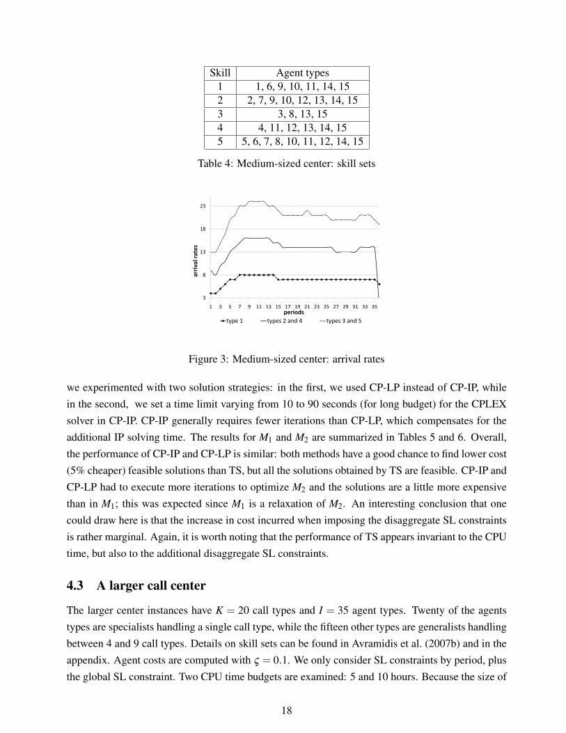
In the medium-sized instances, there are K = 5 call types and I = 15 agent types. Five of the agentstypes are specialists handling a single call type, while the other ten are generalists handling between2 and 5 call types. Details on skill sets can be found in Table 4. The parameter ς used to computeagent costs in formula 4 is now equal to 0.1. Arrival rates for all call types are plotted in Figure 3.

As mentioned earlier, we consider two variants of this example: in M1, only global and per-period SL constraints are enforced, while M2 also includes disaggregate SL constraints. Since inpractice one may find it hard to satisfy all SL constraints and since real-life call center managersare often interested primarily in global SL, it seemed interesting to compare these two variants.For each of them, we performed r = 8 replications for several CPU time budgets of 15, 30 and 60minutes. Because solving the IP instances to optimality would require unacceptable running time,

17

Skill Agent types1 1, 6, 9, 10, 11, 14, 152 2, 7, 9, 10, 12, 13, 14, 153 3, 8, 13, 154 4, 11, 12, 13, 14, 155 5, 6, 7, 8, 10, 11, 12, 14, 15

Table 4: Medium-sized center: skill sets

2323

18

13tes

13

val rat

8arri

33

1 3 5 7 9 11 13 15 17 19 21 23 25 27 29 31 33 35periodsp

type 1 types 2 and 4 types 3 and 5

Figure 3: Medium-sized center: arrival rates

we experimented with two solution strategies: in the first, we used CP-LP instead of CP-IP, whilein the second, we set a time limit varying from 10 to 90 seconds (for long budget) for the CPLEXsolver in CP-IP. CP-IP generally requires fewer iterations than CP-LP, which compensates for theadditional IP solving time. The results for M1 and M2 are summarized in Tables 5 and 6. Overall,the performance of CP-IP and CP-LP is similar: both methods have a good chance to find lower cost(5% cheaper) feasible solutions than TS, but all the solutions obtained by TS are feasible. CP-IP andCP-LP had to execute more iterations to optimize M2 and the solutions are a little more expensivethan in M1; this was expected since M1 is a relaxation of M2. An interesting conclusion that onecould draw here is that the increase in cost incurred when imposing the disaggregate SL constraintsis rather marginal. Again, it is worth noting that the performance of TS appears invariant to the CPUtime, but also to the additional disaggregate SL constraints.

4.3 A larger call center

The larger center instances have K = 20 call types and I = 35 agent types. Twenty of the agentstypes are specialists handling a single call type, while the fifteen other types are generalists handlingbetween 4 and 9 call types. Details on skill sets can be found in Avramidis et al. (2007b) and in theappendix. Agent costs are computed with ς = 0.1. We only consider SL constraints by period, plusthe global SL constraint. Two CPU time budgets are examined: 5 and 10 hours. Because the size of

18

Budget Algorithm n n2 CPUavg Min Med P∗1 P∗ Gperiod(min) sec. cost cost

CP-IP 200 80 764 20.54 20.99 0 62 0.8515 CP-LP 200 80 972 20.29 20.96 0 50 2.33

TS 1000 864 21.47 21.60 0 100 0CP-IP 600 100 1776 20.18 20.51 12 75 0.88

30 CP-LP 600 100 1947 20.36 20.88 0 62 0.74TS 1333 1494 21.43 21.61 0 100 0

CP-IP 1000 400 2981 20.45 20.90 0 62 0.4660 CP-LP 1000 400 2987 20.51 21.26 0 75 0.25

TS 4000 3603 21.49 21.57 0 100 0

Table 5: M1: results obtained with CP-LP and TS for different CPU time budgets

Budget Algorithm n n2 CPUavg Min Med P∗1 P∗ Gperiod Gcall,period(min) sec. cost cost

CP-IP 200 80 664 20.80 21.53 0 37 0.43 0.2115 CP-LP 200 80 1146 20.57 21.81 0 62 0.98 2.28

TS 1000 903 21.47 21.59 0 100 0 0CP-IP 300 80 2188 20.92 21.89 0 62 0.32 0

30 CP-LP 300 80 1827 20.65 21.22 0 62 1.02 0TS 1333 1804 21.47 21.62 0 100 0 0

CP-IP 400 100 3106 20.59 21.26 0 62 0.32 3.3760 CP-LP 400 100 4597 20.71 21.47 0 50 0.17 2.21

TS 4000 3604 21.53 21.59 0 100 0 0

Table 6: M2: results obtained with CP-LP and TS varying the CPU time budget

the problem is too large to run CP-IP efficiently (even with limited IP solving time), we only executeCP-LP and perform r = 8 replications.

One of our objectives with this example is to show that the performance of CP-LP does not dependmuch on the particular structure of the shifts. We thus consider again two variants: L36, which usesthe 9-hour working day and the same shift structure as the previous examples, and L52, which has aworking day starting at 8:00 AM and ending at 9:00 PM; in that variant, the total number of periodsis 52 and all the shifts have a fixed length of 7.5 hours, thus yielding a total of 123 different shifts(considering also shifts starting at 1:00 PM and 1:30 PM in order to cover the additional periods).Arrival rates for the L36 variant and the 36 first periods of L52, follow exactly the same pattern as inthe medium-size example (see Figure 3), with different scalings for the different call types; for L52

they then decrease slowly during the last 16 periods. The results for L36 are displayed in Table 7.Each run of CP-LP has to execute in total around 20,000 simulations. Although the CPU budgets

are several hours, each simulation is actually quite short (averages of 0.7 and 1.3 second/simulationrespectively). CP-LP has difficulty finding feasible solutions, even though constraint violations are

19

Budget Algorithm n n2 CPUavg Min Med P∗1 P∗ Gperiod(hours) min. cost cost

5 CP-LP 400 50 261 79.17 80.05 0 50 0.77TS 4000 268 95.99 100.46 0 100 0

10 CP-LP 500 80 506 78.38 79.44 12 38 0.65TS 6000 602 96.64 100.30 0 100 0

Table 7: L36: results obtained with CP-LP and TS for different CPU time budgets

Budget Algorithm n n2 CPUavg Min Med P∗1 P∗ Gperiod(hours) min. cost cost

5 CP-LP 200 50 300 133.00 133.40 25 37 1.31TS 3000 257 161.50 167.85 0 100 0

10 CP-LP 400 50 696 133.70 134.15 12 25 0.48TS 4400 561 158.60 163.40 0 100 0

Table 8: L52: results obtained with CP-LP and TS for different CPU time budgets

typically very small. TS always finds feasible solutions, but the solutions returned are on average25% more expensive than those obtained with CP-LP. Surprisingly, increasing the CPU budget doesnot improve the performance of TS. This confirms our observations of the previous section regardingthe limited performance of TS. Optimizing periods independently does not seem to lead to a betterscheduling solution. On closer examination of the best scheduling solutions obtained by the twomethods, we find that the CP-LP solution is less expensive because it covers the demand with only52 agents compared to 62 for TS.

The results for the L52 variant are reported in Table 8. On this larger problem, each run of CP-LPhas to execute in total around 35,000 simulations. Because each simulation needs to be short (lessthan 1 second), there is a higher probability of ending up with an infeasible solution. However, theviolation gap decreases as the time budget increases. All the solutions returned by TS were declaredfeasible, but they are 20% more expensive. When we examine the best solutions found by CP-LPand by TS for the L52 instance, we first remark that CP-LP uses only 94 agents compared to 104for TS. We also note that 6 agents in the CP-LP solution are specialists, while there is 1 in the TSsolution. Furthermore, TS uses 32 expensive generalists with 7 skills or more compared to only 22for CP-LP. These three factors combined explain the large difference in cost.

Our motivation for investigating the 52-period example was to verify that CP-LP performed cor-rectly for instances with a different shift structure. Our results confirm this, but at the same timethey highlight one of the potential shortcomings of the approach, which is that, because of simula-tion noise, when there is a large number of constraints, one often ends up with no feasible solution,even though several near-feasible solutions may have been identified. We address this issue next.

20

4.4 Getting more feasible results

Empirical results show that, as problem instances become larger and more complex, there is a defi-nite possibility that CP would return a set of low-cost, but only nearly-feasible solutions. While thismay be acceptable in some practical settings, it is nonetheless annoying to be unable to provide thecall center manager with a solution that meets all his/her requirements. A simple and attractive wayof tackling this problem consists in slightly increasing the right-hand side value of the SL constraintswhen applying the algorithm (except obviously for the final long simulation that is used to determinethe feasibility of solutions). It should be noted that this idea is not specific to the CP procedure andcould therefore be applied with any other solution approach.

We first tested this idea on the L52 instance, using values of 0.81 as target SL for all periods. Wecombined these tests with experiments on the value of the threshold δ used for rounding continuoussolutions to integer ones in CP-LP. The rationale for investigating different values of δ is that therounding procedure introduces a heuristic element in what would otherwise be an exact procedureand that selecting the best value for this threshold is far from obvious.

In our experiments, we considered three different values of δ (0.5, 0.6 and 0.7) for CPU budgetsof 5 and 10 hours, and we ran 8 replications in each case. The chance of obtaining good feasiblesolutions has greatly improved and even had all 8 solutions feasible for one test case. The solutionsalso tend to cost slightly more. The results are summarized in Table 9. These results show that thevalue selected for δ seems to have a small impact on the quality of the solutions obtained. Usinga δ closer to 1 results in a lower incumbent rounded solution in CP-LP and may not represent wellthe incumbent LP solution, in particular when there are few agents per (group,shift)-combination.This can lead to bad cuts in early stages of CP-LP, which happened in the test case δ = 0.7. In fact,it seems to be much more important to make sure that the runs that are made do produce feasiblesolutions, in order to have a larger set to choose from.

δ CPU budget Min Med P∗

hours cost cost0.5 5 133.90 135.35 50

10 133.70 134.85 1000.6 5 133.70 135.00 87

10 134.50 135.15 1000.7 5 139.00 140.20 87

10 136.70 139.15 75

Table 9: L52: results obtained with a target SL of 0.81

We then ran CP-LP with the original 0.80 target value for different values of δ . These testsclearly showed that modifying δ alone was not sufficient to consistently obtain feasible solutions,since more than half of these runs returned infeasible solutions. We also ran the algorithm with a

21

target SL value of 0.81 for the other instances (keeping the value of δ unchanged at 0.5). The resultscan be summarized as follows:

• For the small center, all runs returned feasible solutions (except for very short time budget).The solutions tend to cost slightly more than the ones obtained previously, but a better solutionwas found with a cost of 35.11.

• For the medium-sized instances, almost every run produced a feasible solution, but we did notfind a better solution.

• For the L36 instance, all runs yielded a feasible solution, and we found a better solution with acost of 78.27.

Overall, slightly increasing the value of the SL target value is a useful device for making sure that themethod will return feasible solutions. There is no guarantee that this will provide a better solution,but it may very well do so, especially when there is a large number of constraints. The variabilityof our results highlights once again the stochastic nature of the algorithm, which cannot be avoidedconsidering the significant amount of noise in the simulations.

4.5 The impact of flexibility

We performed another series of numerical experiments to quantify empirically the impact of theflexibility provided by a rich set of shift types. Those experiments were performed on the smallcenter of subsection 4.1. We considered three sets of shift types: the original one with all 285 shifts,a slightly reduced one with 267 shifts, obtained by deleting the 26-period and some 36-period shifts,and adding some 35-period ones, and finally a much more restricted set in which we only allow the105 7.5-hour shifts. The staffing solutions corresponding to the best scheduling solutions obtainedfor these three cases are plotted in Figure 4, along with the optimal staffing solution computed byconsidering each period individually. Three main conclusions can be drawn from this figure:

1. As shown by the solution with 285 shifts, if enough flexibility is introduced in the set ofavailable shifts, it is possible to find schedules that track closely the staffing requirements.

2. Even a slight decrease in flexibility (e.g., by going from 285 to 267 shifts) can lead to asignificant overstaffing in some periods.

3. Schedules with a relatively small number of fixed-length shifts (the 105-shift case) are boundto suffer from major overstaffing.

It follows that, while the complexity of the scheduling problem significantly increases with thenumber of available shifts, there are definite benefits to be reaped from the introduction of morevaried shift types.

22

5 Conclusion

We have proposed in this paper a simulation-based methodology to optimize agent scheduling overone day in a multiskill call center. Even though the use of common random numbers reduces thesimulation noise (or variance) significantly, there is still a fair amount of randomness in the solutionprovided by the algorithm, mainly due to the fact that the simulation length must be kept short(because the estimation of each subgradient requires simulations at up to thousands of differentparameter values). Yet, to our knowledge, better solutions are found with this approach than withany other method we know. In particular, during the development of the cutting plane algorithm, wealso implemented simultaneously a metaheuristic method based on neighborhood search combinedwith queueing approximation, along the lines of Avramidis et al. (2006), but we were unable to makeit competitive for solving the scheduling problem.

In practice, one may run the algorithm a few times (e.g., overnight) to obtain a few solutions andretain the best found. We also showed that by slightly perturbing the SL targets, it is possible toovercome some of the problems caused by the presence of the simulation noise and thus to greatlyincrease the probability of obtaining feasible, high-quality solutions.

Future research on this problem includes the search for faster ways of estimating the subgradi-ents, refining the algorithm to further reduce the noise in the returned solution, and extending thetechnique to simultaneously optimize the scheduling and the routing of calls (via dynamic rules).

Acknowledgements

This research has been supported by Grants OGP-0110050, OGP38816-05, and CRDPJ-320308from NSERC-Canada, and a grant from Bell Canada via the Bell University Laboratories, to the thirdand fourth authors, and a Canada Research Chair to the fourth author. The second author benefitedfrom a scholarship provided jointly by NSERC-Canada, the Fonds quebecois de la recherche sur

33

38

43

48

of agents

13

18

23

28

1 3 5 7 9 11 13 15 17 19 21 23 25 27 29 31 33 35

total num

ber o

periodOptimal Staffing Staffing with 105 shifts Staffing with 267 shifts Staffing with 285 shifts

Figure 4: Small center: staffing solutions with 105, 267 and 285 shift types

23

la nature et les technologies, and Bell Canada. The fifth author benefited from the support of theUniversity of Calabria and the Department of Electronics, Informatics and Systems (DEIS), and herthanks also go to professors Pasquale Legato and Roberto Musmanno.

References

J. Atlason, M. A. Epelman, and S. G. Henderson. Call center staffing with simulation and cuttingplane methods. Annals of Operations Research, 127:333–358, 2004.

A. N. Avramidis, A. Deslauriers, and P. L’Ecuyer. Modeling daily arrivals to a telephone call center.Management Science, 50(7):896–908, 2004.

A. N. Avramidis, W. Chan, and P. L’Ecuyer. Staffing multi-skill call centers via search methods anda performance approximation. Submitted, Revised in May 2007, 2006.

A. N. Avramidis, M. Gendreau, P. L’Ecuyer, and O. Pisacane. Simulation-based optimization ofagent scheduling in multiskill call centers. In Proceedings of the 2007 Industrial Simulation

Conference. Eurosis, 2007a.

A. N. Avramidis, M. Gendreau, P. L’Ecuyer, and O. Pisacane. Optimizing daily agent scheduling ina multiskill call center. Technical report, Publication CIRRELT-2007-44, CIRRELT, Universitede Montreal, Montreal, 2007b.

S. Bhulai, G. Koole, and A. Pot. Simple methods for shift scheduling in multi-skill call centers,2007. Manuscript, available at http://www.cs.vu.nl/~koole/research.

L. Brown, N. Gans, A. Mandelbaum, A. Sakov, H. Shen, S. Zeltyn, and L. Zhao. Statistical analysisof a telephone call center: A queueing-science perspective. Journal of the American Statistical

Association, 100:36–50, 2005.

E. Buist and P. L’Ecuyer. A Java library for simulating contact centers. In Proceedings of the 2005

Winter Simulation Conference, pages 556–565. IEEE Press, 2005.

U. D. o. L. Bureau of Labor Statistics. Occupational Outlook Handbook, Customer Service Rep-

resentatives, 2006-07 Edition. 2007. Available online at http://www.bls.gov/oco/ocos280.htm (last accessed February 14, 2007).

M. T. Cezik and P. L’Ecuyer. Staffing multiskill call centers via linear programming and simulation.Management Science, 54:310–323.

24

CRTC. Final standards for quality of service indicators for use in telephone company regulationand other related matters, 2000. Canadian Radio-Television and Telecommunications Com-mission, Decision CRTC 2000-24. See http://www.crtc.gc.ca/archive/ENG/Decisions/

2000/DT2000-24.htm.

N. Gans, G. Koole, and A. Mandelbaum. Telephone call centers: Tutorial, review, and researchprospects. Manufacturing and Service Operations Management, 5:79–141, 2003.

L. V. Green, P. J. Colesar, and J. Soares. An improved heuristic for staffing telephone call centerswith limited operating hours. Production and Operations Management, 12:46–61, 2003.

S. Halfin and W. Whitt. Heavy-traffic limits for queues with many exponential servers. Operations

Research, 29:567–588, 1981.

S. Henderson and A. Mason. Rostering by iterating integer programming and simulation. In Pro-

ceedings of the 1998 Winter Simulation Conference, volume 1, pages 677–683, 1998.

A. Ingolfsson, E. Cabral, and X. Wu. Combining integer programming and the randomizationmethod to schedule employees. Technical report, School of Business, University of Alberta,Edmonton, Alberta, Canada, 2003. Preprint.

O. B. Jennings, A. Mandelbaum, W. A. Massey, and W. Whitt. Server staffing to meet time-varyingdemand. Management Science, 42(10):1383–1394, 1996.

E. G. Keith. Operator scheduling. AIIE Transactions, 11(1):37–41, 1979.

G. Koole and A. Mandelbaum. Queueing models of call centers: An introduction. Annals of Oper-

ations Research, 113:41–59, 2002.

A. M. Law and W. D. Kelton. Simulation Modeling and Analysis. McGraw-Hill, New York, thirdedition, 2000.

P. L’Ecuyer. SSJ: A Java Library for Stochastic Simulation, 2004. Software user’s guide, Availableat http://www.iro.umontreal.ca/~lecuyer.

P. L’Ecuyer, R. Simard, E. J. Chen, and W. D. Kelton. An object-oriented random-number packagewith many long streams and substreams. Operations Research, 50(6):1073–1075, 2002.

V. Mehrotra. Ringing up big business. ORMS Today, 24(4):18–24, October 1997.

A. Pot, S. Bhulai, and G. Koole. A simple staffing method for multi-skill call centers, 2007.Manuscript, available at http://www.cs.vu.nl/~koole/research.

25

R. Stolletz and S. Helber. Performance analysis of an inbound call center with skill-based routing.OR Spectrum, 26:331–352, 2004.

G. M. Thompson. Labor staffing and scheduling models for controlling service levels. Naval Re-

search Logistics, 8:719–740, 1997.

S. Vogel. A stochastic approach to stability in stochastic programming. Journal of Computational

and Applied Mathematics, 56:65–96, 1994.

26