Embed Size (px)
Citation preview

OPTIMIZING CYCLIC PREFIX LENGTH
FOR DOCSIS 3.1 UPSTREAM
TRANSMISSION
A Thesis Submitted
to the College of Graduate Studies and Research
in Partial Fulfillment of the Requirements
for the Degree of Master of Science
in the Department of Electrical and Computer Engineering
University of Saskatchewan
by
Jing Wang
Saskatoon, Saskatchewan, Canada
c© Copyright Jing Wang, August, 2016. All rights reserved.

Permission to Use
In presenting this thesis in partial fulfillment of the requirements for a Postgraduate degree
from the University of Saskatchewan, it is agreed that the Libraries of this University may
make it freely available for inspection. Permission for copying of this thesis in any manner, in
whole or in part, for scholarly purposes may be granted by the professors who supervised this
thesis work or, in their absence, by the Head of the Department of Electrical and Computer
Engineering or the Dean of the College of Graduate Studies and Research at the University of
Saskatchewan. Any copying, publication, or use of this thesis, or parts thereof, for financial
gain without the written permission of the author is strictly prohibited. Proper recognition
shall be given to the author and to the University of Saskatchewan in any scholarly use which
may be made of any material in this thesis.
Request for permission to copy or to make any other use of material in this thesis in
whole or in part should be addressed to:
Head of the Department of Electrical and Computer Engineering
57 Campus Drive
University of Saskatchewan
Saskatoon, Saskatchewan, Canada
S7N 5A9
i

Abstract
The cable industry originated in United States with the first cable television being in-
vented in 1948. Since the 1990s, many digital devices have been produced and many people
have come to rely on the services provided by cable networks, which has lead to significant
investment in cable network technologies. Interactive programs like GPS, on-line games and
video conferencing, have been introduced in recent years. The customer demands of both
uploading data (upstream) to and downloading data (downstream) from the Internet are
increasing.
There is an international telecommunication standard, DOCSIS, which sets rules for all
cable systems. The latest version DOCSIS3.1 makes a leap forward in technology to offer
larger bandwidth and faster data rates in both upstream and downstream transmissions.
This thesis focuses on one key parameter, cyclic prefix length, of the upstream transmission
system.
The cable modem upstream uses Orthogonal Frequency Division Multiple Access(OFDMA)
for data transmission, which allows a high volume of users to share the whole band at the
same time. Each user occupies a set of sub-carriers for data transmission. The cable mo-
dem transmitter partitions the data into packets that fit into OFDMA frames and sends the
data frames in time sequence to Cable Modem Termination System(CMTS). Different cable
modems in the same frame may have different delays. In each frame, the cyclic prefix is fixed
for all Cable Modems(CMs), and the constellation types can be varied for each CM in order
to achieve the best possible data rate. Therefore, selecting an optimum Cyclic Prefix(CP)
length for the system is an important issue. For all CMs in a frame, if the CP is long enough
to cover the longest delay, the data transmission efficiency will be low. However, if the CP
length is short, some CMs’ performances will be degraded.
To balance the trade-off between the frame length and the signal quality, the purpose of
this research project is to generate a computer program which is able to choose the optimum
CP length for a given cable modem upstream transmission system. The system must obey
the rules set by DOCSIS 3.1.
ii

Several models were built to analyze and corroborate the distribution of interferences
generated by a single sub-carrier when the CP length is insufficient to cover the channel delay.
Finally, a series of mathematical equations, which can successfully estimate the distribution
are developed.
The developed Best CP Length Selection Program is described in detail. The signal
processing procedures and computation methods are explained step by step. The useful
data per minislot was chosen to be the criteria for the program. DOCSIS3.1 allows eleven
CP lengths for the upstream transmission system. By analyzing these allowed CP lengths
and computing the useful data per minislot for each, the best CP length can be determined.
The program was tested for several hypothetical cable networks and generated logical results
in all cases. The results show the Best CP Length Selection Program works properly and is
reliable.
iii

Acknowledgments
I would like to express my thanks to my supervisors, Prof. Brian Daku and Dr. Brian
Berscheid. I really appreciate Prof. Brian Daku who gives me the opportunity to work on
this research topic for Vecima Networks Inc. and he also gives me lots of instructions on
research schedule planning. Dr. Brian Berscheid spends lots of time on my research. He
shows great interests in my work and keeps tracking my process. Thanks for his guidance
throughout my research. He truly gives many valuable comments and suggestions on my
work.
I would also like to thank Prof. Eric Salt. He spends a large amount of his private time
helping me with thesis writing and modifications. I learned many useful writing skills from
him. I really appreciate his work.
I would like to thank all my friends, Yayi, Ben and Chad. I enjoyed lots of interesting and
thoughtful discussions and conversations with them. Thank my boyfriend Xuechao Zhang,
who gives me lots of help and encouragements in my study and life.
Finally, I would like to express my thanks to my parents Qiaolong Wang and Qin Wu.
Thanks for their support and encouragement for the past two years.
iv

Table of Contents
Permission to Use i
Abstract ii
Acknowledgments iv
Table of Contents v
List of Tables ix
List of Figures x
List of Abbreviations xvi
1 Chapter1: Introduction 1
1.1 Cable Industry . . . . . . . . . . . . . . . . . . . . . . . . . . . . . . . . . . 1
1.2 DOCSIS . . . . . . . . . . . . . . . . . . . . . . . . . . . . . . . . . . . . . . 3
1.3 Background . . . . . . . . . . . . . . . . . . . . . . . . . . . . . . . . . . . . 5
1.3.1 CATV Networks . . . . . . . . . . . . . . . . . . . . . . . . . . . . . 5
1.3.2 Distortion in CATV Network . . . . . . . . . . . . . . . . . . . . . . 6
1.3.3 OFDM . . . . . . . . . . . . . . . . . . . . . . . . . . . . . . . . . . . 6
1.3.4 Prefix . . . . . . . . . . . . . . . . . . . . . . . . . . . . . . . . . . . 9
1.3.5 Signal Construction . . . . . . . . . . . . . . . . . . . . . . . . . . . . 12
1.4 Problem Statement . . . . . . . . . . . . . . . . . . . . . . . . . . . . . . . . 13
1.5 Thesis Outline and Main Contributions . . . . . . . . . . . . . . . . . . . . . 17
2 Chapter2: Upstream Transmission System 19
v

2.1 Constellation Mapping . . . . . . . . . . . . . . . . . . . . . . . . . . . . . . 19
2.2 Upstream Transmission System . . . . . . . . . . . . . . . . . . . . . . . . . 22
2.2.1 System Parameters . . . . . . . . . . . . . . . . . . . . . . . . . . . . 24
2.2.2 System Construction . . . . . . . . . . . . . . . . . . . . . . . . . . . 25
2.2.3 Simultaneous Upstream Transmissions . . . . . . . . . . . . . . . . . 27
3 Chapter3: Effects of Interference on a Single Sub-carrier 30
3.1 The Distribution of the Interference Generated by a Single Sub-carrier . . . . 34
3.1.1 Channel Model for Physical Plant . . . . . . . . . . . . . . . . . . . . 34
3.1.2 Sources of Interference . . . . . . . . . . . . . . . . . . . . . . . . . . 35
3.1.3 Calculation of the Distribution of ISISC(K) and ˜IaSISC(K) . . . . . 42
3.1.4 Result . . . . . . . . . . . . . . . . . . . . . . . . . . . . . . . . . . . 44
3.1.5 Effect of Parameter Values . . . . . . . . . . . . . . . . . . . . . . . . 46
3.1.6 Conclusion . . . . . . . . . . . . . . . . . . . . . . . . . . . . . . . . . 53
3.2 Corroboration of the Distribution of the Interference Generated by a Single
Sub-carrier . . . . . . . . . . . . . . . . . . . . . . . . . . . . . . . . . . . . . 53
3.2.1 The Distribution of ISITOTAL(K) . . . . . . . . . . . . . . . . . . . . 53
3.2.2 Result . . . . . . . . . . . . . . . . . . . . . . . . . . . . . . . . . . . 59
3.2.3 Effect of Parameter Values . . . . . . . . . . . . . . . . . . . . . . . . 61
3.2.4 Conclusion . . . . . . . . . . . . . . . . . . . . . . . . . . . . . . . . . 65
3.3 Convolution Model for the Interference . . . . . . . . . . . . . . . . . . . . . 66
3.3.1 Convolution Based Model . . . . . . . . . . . . . . . . . . . . . . . . 66
3.3.2 Results . . . . . . . . . . . . . . . . . . . . . . . . . . . . . . . . . . . 73
vi

3.3.3 Effect of Parameter Values . . . . . . . . . . . . . . . . . . . . . . . . 77
3.3.4 Conclusion . . . . . . . . . . . . . . . . . . . . . . . . . . . . . . . . . 79
3.4 Aggregate Interference Corrupting a Single Sub-carrier . . . . . . . . . . . . 80
4 Chapter4: Best Cyclic Prefix Length Selection 82
4.1 Best CP Length Selection Program Overview . . . . . . . . . . . . . . . . . . 82
4.1.1 Input Parameters to the Program . . . . . . . . . . . . . . . . . . . . 83
4.1.2 Flowchart of the Program . . . . . . . . . . . . . . . . . . . . . . . . 84
4.2 Aggregate Interference Computation . . . . . . . . . . . . . . . . . . . . . . 86
4.3 MER Computation . . . . . . . . . . . . . . . . . . . . . . . . . . . . . . . . 87
4.4 Constellation Type Selection . . . . . . . . . . . . . . . . . . . . . . . . . . . 88
4.4.1 The Usability of BER and MER Plot . . . . . . . . . . . . . . . . . . 91
4.5 Best CP Length Selection . . . . . . . . . . . . . . . . . . . . . . . . . . . . 93
4.6 Program Testing . . . . . . . . . . . . . . . . . . . . . . . . . . . . . . . . . 94
4.6.1 Parameters Used for Testing . . . . . . . . . . . . . . . . . . . . . . . 94
4.6.2 Uniformly Distributed Echo’s Delays . . . . . . . . . . . . . . . . . . 95
4.6.3 Gaussian Distributed Echo’s Delays . . . . . . . . . . . . . . . . . . . 96
4.6.4 Compact Distribution of Echo’s Delays with “Outliers” . . . . . . . . 99
4.6.5 Compact Distribution of Echo’s Delays with Large Mean . . . . . . . 101
5 Chapter5: Discussion and Conclusion 104
5.1 Results Discussion and Further Test . . . . . . . . . . . . . . . . . . . . . . . 104
5.2 Future Work . . . . . . . . . . . . . . . . . . . . . . . . . . . . . . . . . . . . 106
vii

Appendix A DOCSIS 3.1 Table 5-2 108
Appendix B The Main MATLAB Script for the ISI Distribution Simulation
Model 109
Appendix C The Main MATLAB Script for the ISITOTAL Distribution Cor-
roboration Model 112
Appendix D The MATLAB Script for the ISI Distribution Convolution Model115
Appendix E The MATLAB Script for the Aggregate Interference Computa-
tion Function of the Final Model 119
Appendix F The MATLAB Script for the Constellation Order Function of
the Final Model 122
References 124
viii

List of Tables
1.1 The release history of DOCSIS . . . . . . . . . . . . . . . . . . . . . . . . . . 3
1.2 The DOCSIS Upstream Operating Range . . . . . . . . . . . . . . . . . . . . 4
1.3 The DOCSIS 3.1 Downstream Frequency Operating Range . . . . . . . . . . 4
2.1 Constellation types for upstream CM communications . . . . . . . . . . . . . 24
3.1 The parameters for the OFDM system used in the simulation . . . . . . . . . 42
3.2 The parameters for the OFDM system used in the corroboration simulation . 58
3.3 The parameters set for the OFDM system in the corroboration model . . . . 60
3.4 The parameters simulated for the convolution model . . . . . . . . . . . . . 73
4.1 The input parameters for the best cyclic prefix length selection program . . . 83
4.2 The micro-reflections bound for dominant signal echo . . . . . . . . . . . . . 86
4.3 All possible constellation orders for the upstream transmission . . . . . . . . 89
4.4 Parameters used for testing . . . . . . . . . . . . . . . . . . . . . . . . . . . 94
4.5 Number of users for each constellation type for user group 1 . . . . . . . . . 97
4.6 Number of users for each constellation type for user group 2 . . . . . . . . . 99
4.7 Number of users for each constellation type for user group 3 . . . . . . . . . 101
4.8 Number of users for each constellation type for user group 4 . . . . . . . . . 103
5.1 Number of minislots for each constellation type with echo delays uniformly
distributed for BER no larger than 10−20 . . . . . . . . . . . . . . . . . . . . 106
ix

List of Figures
1.1 The time line of cable industry history (extracted from California Cable &
Telecommunications Association Website) [1] . . . . . . . . . . . . . . . . . . 2
1.2 The structure of cable modem communications system [2] . . . . . . . . . . . 4
1.3 CATV network structure, marking the flowing directions of the upstream
signal and its echo . . . . . . . . . . . . . . . . . . . . . . . . . . . . . . . . 5
1.4 Part of the OFDMA system showing how the data blocks transmitted out in
parallel . . . . . . . . . . . . . . . . . . . . . . . . . . . . . . . . . . . . . . . 7
1.5 The structure showing the working principle of Pre-equalizer . . . . . . . . . 9
1.6 OFDM symbols without prefix . . . . . . . . . . . . . . . . . . . . . . . . . . 9
1.7 OFDM symbols with zero prefix and the work procedure of zero prefix . . . 10
1.8 OFDM symbols with cyclic prefix . . . . . . . . . . . . . . . . . . . . . . . . 11
1.9 The OFDM signal structure . . . . . . . . . . . . . . . . . . . . . . . . . . . 12
1.10 The received Signal I, II and III . . . . . . . . . . . . . . . . . . . . . . . . . 13
1.11 Upstream transmission with OFDM frames [3] . . . . . . . . . . . . . . . . . 14
1.12 The delay time distribution of 105 CMs [4] . . . . . . . . . . . . . . . . . . . 15
2.1 QPSK constellation mapping [3] . . . . . . . . . . . . . . . . . . . . . . . . . 20
2.2 16-QAM constellation mapping [3] . . . . . . . . . . . . . . . . . . . . . . . . 21
2.3 128-QAM constellation mapping [3] . . . . . . . . . . . . . . . . . . . . . . . 21
2.4 A simple structure showing the DOCSIS 3.1 upstream transmission system . 23
2.5 The flow chart showing the signal generation procedure in the CM . . . . . . 26
x

2.6 The flow chart showing the procedure in receiver . . . . . . . . . . . . . . . . 27
2.7 The basic signal processing progress of one CM . . . . . . . . . . . . . . . . 28
2.8 The signal produced by one CM . . . . . . . . . . . . . . . . . . . . . . . . . 28
2.9 The structure of signal sent out by upstream transmitters . . . . . . . . . . . 29
3.1 The transmitted signal in a frame consisting of K OFDMA symbols . . . . . 30
3.2 The received signal (The upper plot is the main path; the lower plot is an
echo with delay D, where D is shorter than the length of CP) . . . . . . . . . 31
3.3 The received signal (The upper plot is the main path; the lower plot is an
echo with delay D, where D is longer than the length of CP) . . . . . . . . . 31
3.4 The impulse response of the physical channel linking a CM to the CMTS . . 34
3.5 The block diagram of the physical channel linking a CM to the CMTS . . . 35
3.6 The block diagram of the physical channel used in this study (amplitude and
delay of the main path compensated) . . . . . . . . . . . . . . . . . . . . . . 35
3.7 The sinusoid in one OFDMA symbol . . . . . . . . . . . . . . . . . . . . . . 36
3.8 The OFDMA symbol with cyclic prefix . . . . . . . . . . . . . . . . . . . . . 36
3.9 The received signal which is the sum of the main path and an echo (The echo’s
delay shorter than the length of CP) . . . . . . . . . . . . . . . . . . . . . . 37
3.10 The received signal which is the sum of the main path and an echo (The echo’s
delay longer than the length of CP) . . . . . . . . . . . . . . . . . . . . . . . 38
3.11 The echo in the extraction interval been completed by adding a segment . . 38
3.12 The diagram of the main path signal and an echo with delay D longer than
CP length . . . . . . . . . . . . . . . . . . . . . . . . . . . . . . . . . . . . . 39
xi

3.13 The echo in the extraction interval been completed by adding a segment and
include the previous symbol’s echo . . . . . . . . . . . . . . . . . . . . . . . 40
3.14 The structure of the transmitted signal . . . . . . . . . . . . . . . . . . . . . 43
3.15 The received signal with one main path and an echo with delay D and mag-
nitude Ae . . . . . . . . . . . . . . . . . . . . . . . . . . . . . . . . . . . . . 43
3.16 The received main path and the echo scaled in unit of samples . . . . . . . . 44
3.17 ISI distribution with NCP =256, echo delay D=500, echo magnitude Ae =
−16dB and the only non-zero sub-carrier SC-74 . . . . . . . . . . . . . . . . 45
3.18 IaSI distribution with NCP =256, echo delay D=500, echo magnitude Ae =
−16dB and the only non-zero sub-carrier SC-74 . . . . . . . . . . . . . . . . 46
3.19 ISITOTAL distribution with NCP =256, echo delay D=500, echo magnitude
Ae = −16dB and the only non-zero sub-carrier SC-74 . . . . . . . . . . . . . 47
3.20 ISI distributions comparison between the length of the cyclic prefix NCP =
96 and 256 . . . . . . . . . . . . . . . . . . . . . . . . . . . . . . . . . . . . . 48
3.21 ISI distributions comparison between the echo’s delay D= 500 and 1000 . . 49
3.22 ISI distributions comparison between the echo’s magnitude Ae = −16dB and
−35dB . . . . . . . . . . . . . . . . . . . . . . . . . . . . . . . . . . . . . . . 50
3.23 ISI distributions comparison between QPSK and 16-QAM systems . . . . . 52
3.24 The transmitted constellation of QPSK . . . . . . . . . . . . . . . . . . . . . 54
3.25 The transmitted constellation and the reference constellation of QPSK . . . 56
3.26 The transmitted constellation, the reference constellation and the received
constellation of QPSK . . . . . . . . . . . . . . . . . . . . . . . . . . . . . . 56
xii

3.27 Distribution of ISITOTAL comparing the results of simulation model to cor-
roboration model for NCP=256, echo’s delay D=500, Echo’s magnitude Ae =
−16dB, QPSK modulation type and a single non-zero sub-carrier, SC-74.
Left: Full frequency range
Right: Zoomed on Sub-carrier 74 . . . . . . . . . . . . . . . . . . . . . . . . 60
3.28 Distribution of ISITOTAL comparing the results of simulation model to cor-
roboration model for NCP=96, echo’s delay D=500, Echo’s magnitude Ae =
−16dB, QPSK modulation type and a single non-zero sub-carrier, SC-74. . . 61
3.29 Distribution of ISITOTAL comparing the results of simulation model to cor-
roboration model for NCP=256, echo’s delay D=1000, Echo’s magnitude Ae =
−16dB, QPSK modulation type and a single non-zero sub-carrier, SC-74. . . 63
3.30 Distribution of ISITOTAL comparing the results of simulation model to cor-
roboration model for NCP=256, echo’s delay D=500, Echo’s magnitude Ae =
−35dB, QPSK modulation type and a single non-zero sub-carrier, SC-74. . . 64
3.31 Distribution of ISITOTAL comparing the results of simulation model to cor-
roboration model for NCP=256, echo’s delay D=500, Echo’s magnitude Ae =
−16dB, 16-QAM modulation type and a single non-zero sub-carrier, SC-74. . 65
3.32 The diagram of the main path signal and an echo with delay D longer than
CP length . . . . . . . . . . . . . . . . . . . . . . . . . . . . . . . . . . . . . 67
3.33 The signal in extraction interval for OFDMA Symbol 2 . . . . . . . . . . . . 67
3.34 Top Plot: The echo portion in the extraction interval;
Bottom Plot: OFDMA Symbol 1. . . . . . . . . . . . . . . . . . . . . . . . . 68
3.35 The structure of the extracting mask designed to extract the ISI segment . 68
3.36 Apply circular shift to the OFDMA Symbol 1 . . . . . . . . . . . . . . . . . 69
xiii

3.37 Transfer the extracting mask from time domain to frequency domain;
Left side: Extracting mask in time domain;
Right side: Extracting mask in frequency domain. . . . . . . . . . . . . . . . 70
3.38 The OFDMA Symbol 1 in frequency domain . . . . . . . . . . . . . . . . . . 71
3.39 The largest case: when the echo is in phase with respect to the signal in the
main path . . . . . . . . . . . . . . . . . . . . . . . . . . . . . . . . . . . . . 72
3.40 The smallest case: when the echo is 180 degree out of phase with respect to
the signal in the main path . . . . . . . . . . . . . . . . . . . . . . . . . . . . 73
3.41 Distribution of ISI for the largest case. Comparing the results of simulation
model to convolution model for NCP=256, echo’s delay D=500, Echo’s mag-
nitude Ae = −16dBand a single non-zero sub-carrier, SC-74.
Left: Full frequency range
Right: Zoomed on Sub-carrier 74 . . . . . . . . . . . . . . . . . . . . . . . . 74
3.42 Distribution of ISI for the smallest case. Comparing the results of simulation
model to convolution model.
Left: Full frequency range
Right: Zoomed on Sub-carrier 74 . . . . . . . . . . . . . . . . . . . . . . . . 75
3.43 Distribution of ISI for the average case. Comparing the results of simulation
model to convolution model.
Left: Full frequency range
Right: Zoomed on Sub-carrier 74 . . . . . . . . . . . . . . . . . . . . . . . . 76
3.44 Distribution of ISI comparing the results of simulation model to convolution
model for NCP=96, echo’s delay D=500, Echo’s magnitude Ae = −16dB and
a single non-zero sub-carrier, SC-74. . . . . . . . . . . . . . . . . . . . . . . . 78
3.45 Distribution of ISI comparing the results of simulation model to convolution
model for NCP=256, echo’s delay D=1000, Echo’s magnitude Ae = −16dB
and a single non-zero sub-carrier, SC-74. . . . . . . . . . . . . . . . . . . . . 79
xiv

3.46 Distribution of ISI comparing the results of simulation model to convolution
model for NCP=256, echo’s delay D=500, Echo’s magnitude Ae = −35dB and
a single non-zero sub-carrier, SC-74. . . . . . . . . . . . . . . . . . . . . . . . 80
4.1 Flow chart of the working process of the Best CP Length Selection Program 85
4.2 MER in dB vs. BER plot for all possible constellation orders . . . . . . . . . 90
4.3 An example to show how to choose a suitable constellation type . . . . . . . 91
4.4 The histograms of errors in active sub channel for QPSK with NCP=256,
D=500, Ae=-16dB . . . . . . . . . . . . . . . . . . . . . . . . . . . . . . . . 92
4.5 Distribution of echo’s delay in user group 1 . . . . . . . . . . . . . . . . . . . 95
4.6 The useful data per minislot for user group 1 . . . . . . . . . . . . . . . . . . 96
4.7 Distribution of echo’s delay in user group 2 . . . . . . . . . . . . . . . . . . . 97
4.8 The useful data per minislot for user group 2 . . . . . . . . . . . . . . . . . . 98
4.9 Distribution of echo’s delay in user group 3 . . . . . . . . . . . . . . . . . . . 100
4.10 The useful data per minislot for user group 3 . . . . . . . . . . . . . . . . . . 100
4.11 Distribution of echo’s delay in user group 4 . . . . . . . . . . . . . . . . . . . 102
4.12 The useful data per minislot for user group 4 . . . . . . . . . . . . . . . . . . 102
5.1 The useful data ratio per minislot for each CP length with BER requirement
to be 10−20 . . . . . . . . . . . . . . . . . . . . . . . . . . . . . . . . . . . . 105
A.1 Table 5 2 - Typical Upstream RF Channel Transmission Characteristics . . 108
xv

List of Abbreviations
AWGN Additive White Gaussian Noise
BER Bit Error Rate
BPSK Binary Phase Shift Keying
CATV Cable Television
CM Cable Modem
CMTS Cable Modem Termination System
CP Cyclic Prefix
DFT Discrete Fourier Transform
DOCSIS Data Over Cable Service Interface Specification
FEC Forward Error Correction
FFT Fast Fourier Transform
LDPC Low-Density Parity-Check
IaSI Intra Symbol Interference
ICI Inter Carrier Interference
IDFT Inverse Discrete Fourier Transform
IFFT Inverse Fast Fourier Transform
ISI Inter Symbol Interference
MAC Media Access Control
MATLAB Matrix Laboratory
MER Modulation Error Ratio
OFDM Orthogonal Frequency-Division Multiplexing
OFDMA Orthogonal Frequency-Division Multiple Access
QAM Quadrature Amplitude Modulation
QPSK Quadrature Phase Shift Keying
RP Roll-off Period
SC Sub-Carrier
SER Symbol Error Rate
SNR Signal Noise Ratio
xvi

1. Chapter1: Introduction
1.1 Cable Industry
Cable television originated in United States in 1948 [5] and later transitioned into broad-
band cable communications. A cable modem is a type of bridge, connecting users’ devices to
the Internet [6]. Figure 1.1 shows the evolution time line of cable network industry. In 1990s,
the capacity of cable networks had to expand to accommodate new digital services, including
cable telephone, high-speed Internet, high definition TV and digital recorders. People are
more and more dependent on the digital services provided by cable networks, which leads to
the cable industry expanding bandwidth and offering more services.
Initially, the cable network was a one-way data transmission system. It was a broadcast
system, where signals are unidirectional and transmitted from a central point to all users [7].
Interactive programs are among the recently introduced services. In the recent years,
there are lots of applications which require interaction between users and the Internet, like
GPS, on-line games and video conferencing [8]. The demand for users to upload data to the
Internet is ever increasing. Therefore, the cable network is increasing the bandwidth of the
upstream communication for uploading data from users to the Internet.
The demands of uploading data to and downloading data from the Internet are still
increasing [9]. The latest standard DOCSIS 3.1, makes a leap forward in technology to offer
larger bandwidth and faster data rates in both the upstream and downstream directions.
The standard will be discussed in Section 1.2. To meet this standard, a new cable modem
system must be designed. This thesis will focus on one of the key issues in the upstream
communication link.
1

Figure 1.1 The time line of cable industry history (extracted from California Cable
& Telecommunications Association Website) [1]
2

Table 1.1 The release history of DOCSIS
Version Year
DOCSIS 1.0 1997
DOCSIS 1.1 1999
DOCSIS 2.0 2001
DOCSIS 3.0 2006
DOCSIS 3.1 2013
1.2 DOCSIS
DOCSIS which is short for Data Over Cable Service Interface Specifications, is an in-
ternational telecommunications standard set for all cable systems [3]. DOCSIS is developed
and released by CableLabs, which is a consortium of cable network, operators and equipment
suppliers, including 3Com, BigBand Networks and Cisco.
There are many manufacturers producing cable modems and cable modem termination
systems. Customers can buy a cable modem from a manufacturer of their choice. To
make sure different brands’ cable modems are able to communicate with the cable modem
termination system (CMTS), all the manufacturers must obey the rules set by DOCSIS.
With the increasing user demand, CableLabs also keeps updating DOCSIS by setting new
bandwidth, modulation types and other communication techniques. Table 1.1 shows the
releasing history of DOCSIS.
DOCSIS 3.1 was released in 2013 and updated several times. The most recent modifica-
tion is December, 2014.
A CATV communication system provides a gateway between a cable modem in sub-
scribers residence and the Internet. The basic structure for a CATV communication system
is shown in Figure 1.2 . A CATV communication system can be separated into three parts:
the CMTS, the cable plant and the Cable Modem (CM). The CMTS is a transfer station,
communicating with both CM and Internet to help organize and satisfy all the requests [10].
The CMTS can be further separated into two parts: the Media Access Control (MAC)
3

Figure 1.2 The structure of cable modem communications system [2]
Table 1.2 The DOCSIS Upstream Operating Range
Lower Band Edge Upper Band Edge
5MHz 204MHz
Layer and the Physical Layer [11]. The MAC layer is the software responsible for arranging
the signal transmission sequence, setting parameters for things like the Cyclic Prefix (CP)
length and all the programmable logic. The Physical Layer is responsible for modulating the
transmitted data, demodulating the received data and all other logic built in hardware.
The communication between the CM and the CMTS is two-way. Data transferred from
the CM to the CMTS uses upstream bandwidth, and data transferred from the CMTS to
the CM uses downstream bandwidth. Table 1.2 shows the DOCSIS upstream frequency
operating range, which is from 5MHz to 204MHz. Table 1.3 shows the DOCSIS downstream
frequency operating range, which must support frequency from 258MHz to 1218MHz and
should allow the frequencies from 108MHz to 1794MHz [12].
Since users download much more things from the Internet, the downstream bandwidth
is much wider than the upstream one. However, with the increasing use of interaction
Table 1.3 The DOCSIS 3.1 Downstream Frequency Operating Range
Requirement Lower Band Edge Upper Band Edge
MUST 258MHz 1218MHz
SHOULD 108MHz 1794MHz
4

Figure 1.3 CATV network structure, marking the flowing directions of the up-
stream signal and its echo
like games, the demand of uploading data is increasing. To accommodate this increasing
demand, DOCSIS 3.1 expands the upstream bandwidth from 5-85MHz to 5-204MHz and
switches from single carrier QAM to OFDM modulation. The implication is a new upstream
system must be developed for DOCSIS 3.1.
1.3 Background
1.3.1 CATV Networks
CATV is commonly known as cable TV. CATV networks do not only deliver TV pro-
grams, but also Internet service. Therefore, the communication between the CMs and the
CMTS is two-way. In this research project, only the upstream transmission system, which
is transmission from the CM to the CMTS will be considered.
In the upstream transmission system, cable modems connect to the users’ devices and
collect data from them. Coaxial cable transfers the users’ data to the CMTS and the CMTS
is responsible for interfacing to the Internet. The structure of the CATV network in shown
in Figure 1.3 .
5

1.3.2 Distortion in CATV Network
In the coaxial cable network, a directional coupler [13] is used to extract some power from
the downstream transmission and send to the CM, and direct the signal generated by the
CM in the upstream direction. These couplers are shown in Figure 1.3, as the dots labelled
Coupler 1 and Coupler 2.
All the components are attached to the system with connectors. At each connection
point, there is a probability of an impedance mismatch. Usually, connectors are perfectly
matched and will not cause signal distortion. An imperfect connector passes most of the
signal power through and reflects the rest power back. Therefore, once a signal is sent out,
it will be reflected at imperfect connectors. The main signal with most power will continue
transmitting in the original direction and the reflected signal will travel in the opposite
direction. When the reflected signal encounters a mismatched connector, a portion of it is
reflected. This second reflection now travels in the same direction as the original signal and
is referred to as an echo.
Figure 1.3 shows part of the signal flowing in the upstream transmission. Cable modem
1 sends out Signal 1. When reaching Coupler 1, the signal is attenuated by the tap gain
and sent in the direction of the CMTS. This signal is shown in Figure 1.3 as Signal 2.
Unfortunately, the directional couplers are not perfect and some of the signal from CM 1 is
sent downstream. This downstream component is typically 20dB below the original signal.
The signal is shown in Figure 1.3 as Signal 3. Now suppose there is a bad connector on
Coupler 2. This will cause Signal 3 to be reflected back toward the CMTS. The reflected
portion of Signal 3 is shown as Signal 4 in Figure 1.3. Signal 4 keeps transmitting in the
toward CMTS direction. Signal 4 is slightly attenuated by the insertion loss of Coupler 1 to
become Signal 5. Signal 5 is received by the CMTS as an echo.
1.3.3 OFDM
OFDM is short for orthogonal frequency-division multiplexing. It is a modulation method
to encode data on multiple carrier frequencies for high data rate transmission [14]. In the past
6

Figure 1.4 Part of the OFDMA system showing how the data blocks transmitted
out in parallel
few years, OFDM has been increasingly emphasized on applications to worldwide telecom-
munication networks, especially the 4G and wifi networks [15].
OFDMA is short for orthogonal frequency-division multiple access. It is a multi-user
version of the OFDM modulation. In an OFDMA system, high volume of data is to be
transmitted over a large number of low rate carriers. The carriers are orthogonal to each
other and the frequency space between them is decided by the size of the Fourier Transform
[16]. Each of the sub-carriers is able to transmit data independently. At the receiver, the
demodulator will recover all signals and separate them according to frequencies. Therefore,
OFDMA method allows a large amount users to share the frequency band and transmit data
in parallel.
Take the system in Figure 1.4 for example. It is a 2k FFT system with 2048 sub-carriers
in total and the active sub-carriers are from 74 to 1973. The inputs to this system are 1900
independent data sources. As Figure 1.4 shows, the three data blocks can be transmitted
at the same time by assigning them to different sub-carriers. Equation 1.1 explains the
procedure in a mathematical way.
x(n) =1√N
N−1∑k=0
X(k)ej2πnkN , 0 ≤ n ≤ N − 1, (1.1)
The operation shown in equation 1.1 is an Inverse Fast Fourier Transform(IFFT), which
7

converts the signals in frequency domain to time domain. Therefore, the output of equa-
tion 1.1 is a time domain OFDM symbol array. A more detailed description of an OFDM
system is given in Chapter 2.
In an OFDM system, the useful information is coded into the amplitude and phase of each
sub-carriers. Therefore, the aim of system is to precisely recover the amplitude and phase
of the received signals at each frequency. Imagine a perfect system where signal Aej(ωt+θ) is
sent out through the transmitter. The transmitted signal has amplitude A, phase shift θ in
the unit of radians and angular frequency ω in the unit of radians per second.
Transmitted−signal = Aej(ωt+θ); (1.2)
Ideally, at the demodulator, the recovered signal will be the same as the transmitted
signal. Because of the transmission distortion, when the signal arrives at the receiver, it will
always be delayed and attenuated comparing to the transmitted one, which can be expressed
as
Main−signal = A1ej(ω(t−τ)+θ); (1.3)
Where A1 is the received amplitude of the main signal, τ is the delay in the unit of second.
However, when an echo exists, the received signal is the sum of the main signal and the
echo, as Equation 1.4 shows.
Received−signal = A1ej(ω(t−τ)+θ) + Aee
j(ω(t−te)+θ) (1.4)
Where Ae is the amplitude of the echo and te is the echo’s delay compare to the trans-
mitted signal. Since an echo is just a repetition of the original signal with less power, the
phase shift of the driving signal θ still remains the same.
For each sub channel, the frequency response is a constant. By comparing the received
signal with the transmitted signal, the distortion percentage can be computed. To make the
amplitude and phase of the received signal the same as the one transmitted, a pre-equalizer
is added to the system. As Figure 1.5 shows, the pre-equalizer adjusts the amplitude and
phase of the original signal before it is sent out. Then with the effect of echo in this sub-
8

Figure 1.5 The structure showing the working principle of Pre-equalizer
Figure 1.6 OFDM symbols without prefix
carrier, the received signal is still the same as the original one. The pre-equalizer helps to
compensate for the signal distortion caused by the echo.
However, the pre-equalizer only works well when the received echo is still a complete
sinusoid, which can be expressed as the component in Equation 1.4. Once the echo is not
a full sinusoid or some other signals are included, because of these interferences, the pre-
equalizer cannot compensate for the distortion in the received signal. To make the echo to
be a full sinusoid, cyclic prefix should be included, which is introduced in the next section.
1.3.4 Prefix
As discussed in Section 1.3.3, the signal sent out by the transmitter is an array of OFDM
symbols. Figure 1.6 shows two adjacent OFDM symbols. To make it easy to understand, the
two OFDM symbols are constructed as single sinusoids, but with different frequencies. The
upper plot is the main transmitted signal and the lower one is an echo. The demodulator
will detect and extract the OFDM symbol from the received signal. The extraction interval
9

Figure 1.7 OFDM symbols with zero prefix and the work procedure of zero prefix
depends on the location of the main transmitted signal. Therefore, the area between red
dashed lines will be extracted by the demodulator for signal recovery. It can be seen that,
once there is an echo, no matter how short the delay, part of the previous symbol will fall into
the current extraction interval, as the red curve of each symbol shows in Figure 1.6. Part
of the current echo will fall into the subsequent extraction interval. Therefore, the current
echo is no longer a completed sinusoid and the echo from the previous sinusoid is shifted into
the extraction interval. The portion of the echo shifted into the extraction interval from the
echo of the previous signal is called Inter Symbol Interference (ISI). The missing portion of
the self echo is also interference. It is called Intra Symbol Interference (IaSI). Both type of
interference can be avoid by inserting a prefix in front of each symbol.
The prefix is a guard interval between OFDM symbols to separate them with the purpose
of avoiding (if the guard interval is large enough) or reducing (if the guard interval is not
large enough) the effect of echo.
There are two possibilities for prefix: one of all zeros and the other being a cyclic extension
time domain OFDM signal. The all-zero prefix is illustrated in Figure 1.7 . Each time domain
symbol is preceded with a sequence of zeros. Still, the extraction interval is set to extract
10

Figure 1.8 OFDM symbols with cyclic prefix
the main signal, which is the interval between the red dashed lines. As the middle plot
of Figure 1.7 shows, the echo from the previous symbol does not shift through the guard
interval and reach the extraction interval. Therefore, there is no ISI. However, there is still a
sequence of the self echo missing in the extraction area. This missing piece can be replaced by
adding the guard interval that follows a symbol to the beginning of the extraction interval.
The cut-and-paste procedure is described in the last plot of Figure 1.7. The green curve
which is outside of the extraction interval in the middle plot is moved and attached to the
front of the symbol. This makes the echo a complete sinusoid in the extraction interval and
eliminate the IaSI.
A cyclic prefix is constructed by repeating the end of an OFDM symbol and adding it to
the front of each symbol to form a guard interval of a different sort [17]. Figure 1.8 shows the
structure of cyclic prefixed signal and the magenta curves appended to the OFDM symbols
are cyclic prefix. The lower plot is an echo of the signal. With the delay, part of the symbol
falls out and part of the cyclic prefix falls into the extraction interval. Since the cyclic prefix
is a repetition of part of the symbol, it still remains a full sinusoid. Therefore, no interference
will be introduced in this case. However, if the delay is longer than the cyclic prefix, it is
another story, which will be introduced in the next section.
To ensure the quality of the OFDM signal transmission, each OFDM symbol must be
prefixed. In DOCSIS 3.1 and therefore in this research, cyclic prefix separates the OFDM
11

Figure 1.9 The OFDM signal structure
symbols. Should the cyclic prefix be long enough, both ISI and IaSI can be completely
removed.
1.3.5 Signal Construction
To maximize the channel capacity, the time domain symbol is windowed to sharpen the
edges of the OFDM signal spectrum [18]. For the windowing purpose, a cyclic suffix called
roll-off period(RP) [19] is appended to the end of OFDM symbol.
The upper diagram in Figure 1.9 shows two complete signals constructed with CP, OFDM
symbol and RP. The transmission of a subsequent signal starts at the beginning of the RP.
That is the RP of one symbol overlap the CP of the following symbol. For ease of drawing
the RP of the previous symbol, RP is considered part of the CP of the next signal as shown
at the bottom of Figure 1.9.
In the case of the signal reflection discussed in Section 1.3.2, after the upstream demodu-
lator receives the main transmitted signal, it will receive attenuated echo signals. Figure 1.10
is a reduced diagram showing the main transmitted Signal I, the reflected Signal II and III
with different echo delays D1 and D2. Assume D1 is shorter than CP length and D2 is longer
than CP length.
The red box area shown in Figure 1.10 is one of the extraction intervals of the demodu-
lator. For Signal II, the CP length is longer than the delay D1. Part of the cyclic prefix data
and echo signal will be extracted by the demodulator. According to the working principle
of cyclic prefix, the extracted signal is still a full sinusoid, which will not cause noise for the
12

Figure 1.10 The received Signal I, II and III
signal recovery.
For Signal III, delay D2 is longer than the CP length. Not only the whole cyclic prefix
portion, but also part of the previous symbol will be shifted to the extraction interval. The
extracted echo signal is a combination of two sinusoid with different frequencies. It is no
longer a completed sinusoid orthogonal to the main symbol. The noise introduced is called
inter symbol interference, or ‘ISI’ for short. In the upstream transmission system, there
are two kinds of ISI, Self-echo ISI and Simultaneous ISI. More detailed description and
explanation of these type will be given in Chapter 3.
1.4 Problem Statement
The cable modem upstream transmitter partitions the data into packets that fit into
OFDM frames and sends the data frame by frame to CMTS. As Figure 1.11 shows, the
OFDM frames are sent out in time sequence. Each frame has the same duration and occupies
the entire active upstream spectrum. For example, with 50kHz sub-carrier spacing, the
upstream spectrum is occupied with 2048 sub-carriers in total. Only sub-carriers numbered
from 74 to 1973 are active, the rest form guard bands in the frequency domain. A group
of Q contiguous sub-carriers, where Q could be 8 or 16, form a minislot. OFDM frames
are shared by CMs. Each of the CMs is assigned one or more separate minislots. Once the
13

Figure 1.11 Upstream transmission with OFDM frames [3]
length of the cyclic prefix is chosen, it is the same for all symbols and can not be set on a
minislot basis to match a particular CM. However, the modulation order can be set on a
minislot by minislot basis to match the quality of the channel of the CM assigned to the
minislot.
Cable modems are connected to the CMTS through different channels that may have
strong or weak echos and more or less noise. Therefore, different minislots in the same frame
might have different echo delays. Since the CP length is fixed for all minislots, for some the
length of the CP may be excessive and for others it may be too short. Choosing the best
length for the CP is an important issue. On one hand, if the CP length is long enough to
avoid ISI in all minislots, i.e. sized for the worst case CM, the data transmission efficiency
will be low. On the other hand, if the CP length is shorter than the echo delay for a few
CMs, ISI will result, and the performance of these CMs will be degraded.
This sets up a trade-off between frame length and signal quality. Since the cyclic prefix
14

Figure 1.12 The delay time distribution of 105 CMs [4]
does not contain any useful information, it is overhead and should be kept to a minimum.
However, if the CP is short, it causes ISI and increases the error rate for some CMs. A
detailed analysis is given with an example below.
Figure 1.12 is a histogram of the echo delay for 105 CMs in a hypothetical network. The
shape of the distribution is referred to the analysis of real applications [4]. Most of the CMs
have echo delays shorter than 3µs. Only 13 out of 105 CMs have echo with delays between
3µs and 6µs. The trade-off is: If the CP is sized for the worst case echo, i.e. set to be 6µs,
as indicated by the dash line on the right(green) in Figure 1.12, the length of the CP will
be longer than the delay of the longest echo. No ISI will exist for any CM, which is perfect
for signal quality. However, most CMs don’t need such a long CP to have perfect signal
qualities. A shorter CP length is enough for them to make perfect transmission without any
ISI. Therefore, if the cyclic prefix is longer than necessary for most CMs, the cost of the extra
overhead is born by all. Clearly if the cyclic prefix is shortened, the order of modulation
would have to be reduced in some CMs, which means they would need more minislots to
transmit their data. Of course, this reduces transmission efficiency.
15

If CP length is set to be 3µs, in the place where the dash line on the left (red) is, CMs
with echo delays shorter than 3µs (92 out of 105) will not generate ISI in the receiver. 13
users will experience lower quality transmission. However, the transmission efficiency may
be higher when the shorter CP length is used. Actually, the 13 users suffering from ISI
can be assigned lower order modulation, to reduce the bit error rate to a safe range. Lower
modulation order means lower data rate, but to ensure the transmission quality, lower data
rate for limited CMs is acceptable. In this case, the 3µs CP seems to be a reasonable choice.
Nevertheless, it might not be the best one. The best choice is the one that maximizes system
throughput.
The aim of this thesis is to develop a technique to find the best CP length for an upstream
transmission system. The intent is to maximize through put by balancing the transmission
efficiency and quality. The performance measure used to evaluate the transmission perfor-
mance is the average data throughput.
The best choice for the CP length depends on the distribution of echo delay, echo magni-
tudes, as well the bit error rate (BER) requirement. Different CATV systems have different
characteristics, so the input parameters will be different. In this research, the input param-
eters are defined by the researcher, just for test. However, the technique could apply to
any DOCSIS system, analyzing the stored users’ information and then suggesting a best CP
length.
The research content introduced in this thesis is meant to be a ‘model of concept’. Some
factors are ignored to make the main idea more clear and logical. The bit error rate considered
in this thesis is the one before low-density parity-check (LDPC) is applied. For future study,
all the missed details can be added to make the model more exact.
To achieve the final purpose, the research is conducted step by step. It starts with a simple
model to explore the effect of the length of the CP on the ISI distribution in frequency and
modulation error ratio (MER) of each sub-carrier. The model is sufficiently accurate to
determine the sensitivity of data throughput to the length of the CP.
16
1.5 Thesis Outline and Main Contributions
The thesis has five chapters in total.
Chapter 1 first introduces some background information, including the cable modem
industry, DOCSIS and its released history. Then, to better explain the purpose of this
thesis, some background knowledge about cable modem upstream transmission is included.
The introduction of the working principles of the CATV networks and the distortion in
CATV networks gives a general idea about CATV networks. The knowledge of OFDM,
prefix and signal construction can help to explain the existing problem. Finally, the purpose
and the desired results of this research project are also described in Section 1.4. A computer
program which is able to choose the optimum CP length for the cable modem upstream
transmission system is expected to be generated in this research. The system must obey the
rules set by DOCSIS 3.1.
Chapter 2 introduces some basic concepts of an OFDM system in order to give some
general idea to readers who are not familiar with wire line communication. Modulation and
constellation mapping are introduced first and followed by the OFDM system construction.
The OFDM system is the most basic model used in the research. Therefore, a detailed
explanation of the OFDM system is given, including the transmitter, channel and receiver.
In Chapter 3, the effects of interference on a single sub-carrier is studied. In a practical
system, Inter Symbol Interference (ISI) which is caused by neighbouring symbols and Intra
Symbol Interference (IaSI) which is caused by self inflicted, will be introduced into the
upstream transmission system. To study the distribution of the interference of a single sub-
carrier among all other sub-carriers, the sources of the two interferences are analyzed and
the theoretical computation methods are discussed. Finally, a model based on detecting
the sources of the interference is generated and the interference distribution is plotted. The
effect of some relevant parameters, including CP length, echo’s delay, echo’s magnitude and
modulation order are also studied.
To corroborate the analysis of the interferences in the first model, a corroboration model
is built based on analyzing the constellation points constructed from the received signal and
17

finding the error caused by the interference. The results and plots of the corroboration model
proves the analysis of the sources of the interferences in the first model is correct.
The identified and corroborated sources will be used in the convolution model, which
is developed to estimate the distribution of the interferences of a single sub-carrier. The
convolution model contains a series of mathematical expressions, including the convolution
of a symbol with a mask. The distribution of the interferences plotted by the convolution
model matches the corroboration model well. Therefore, a series of mathematical equations,
which can successfully estimate the distribution of interference of a single sub-carrier, are
developed and this is one of the contributions of this thesis.
The distribution of interferences of a single sub-carrier is estimated with the convolution
model. The variable of interest is the aggregate interference corrupted in each sub-carrier
and the computation method is also given in Chapter 3.
Based on all the work done in previous chapters, Chapter 4 introduces the Best CP
Length Selection Program in detail. The overview and the inputs and output of the pro-
gram are described first to give a general idea. Then, the signal processing procedures are
introduced step by step. The criteria used to assess the program is the useful data per
minislot. DOCSIS3.1 allows eleven CP lengths for the upstream transmission system. The
program is run iteratively for each of these CP options. The one giving the best useful data
per minislot will be selected to be the optimum CP for the system. The program is tested
with four different distributions of users and delays. The results show the Best CP Length
Selection Program works properly.
Chapter 5 discusses the results from Chapter 4 and some further tests are made on the
program to make sure the program is reliable. Based on the current developed Best CP
Length Selection Program, the future work is also discussed in this chapter.
The appendices mainly include some necessary Matlab codes for this project.
18

2. Chapter2: Upstream Transmission System
A simple cable modem upstream transmission system, including transmitter, channel and
receiver will be introduced in this chapter.
Before describing the principle of the system, some concepts about modulation and con-
stellation mapping will be introduced. These concepts will be used in describing the system.
2.1 Constellation Mapping
Modulation is the variation of one or more properties of an RF signal such as frequency,
amplitude and phase in order to represent data [20]. There are basic digital modulation
formats like FSK (Frequency-shift keying), ASK (Amplitude-shift keying) and PSK (Phase-
shift keying) [21]. QAM (Quadrature Amplitude Modulation) is also a kind of modulation,
which modulates the amplitudes of two carrier waves which have the same frequency and
are 90 degrees out of phase [22]. DOCSIS upstream channels use the QAM modulation
technique.
In order for successful communication to occur, the transmitter and receiver need to agree
upon how a set of message data bits will be used to vary the properties of an RF carrier
signal. The typical approach is to group multiple data bits together, then modulate the RF
signal in a specific way, depending on the values of the data bits. A mapping rule is specified
which defines the symbol (modulated waveform) to be transmitted for each possible set of
data bits.
To illustrate this concept, a constellation mapping diagram can be used to represent the
modulation. For QAM, the constellation mapping diagram contains a real (or I, which stands
19

Figure 2.1 QPSK constellation mapping [3]
for in-phase) axis and an imaginary (or Q, which stands for quadrature) axis. These axes
are used to build a Cartesian coordinate space. Each of the possible transmitted symbols
can be mapped to a point in the I and Q space. A variety of different mapping rules are
possible. In general, a mapping rule which includes M possible symbols is referred to as an
M-QAM constellation. The amplitude and phase of each point in the constellation diagram
indicates the amplitude and phase with which the RF carrier is modulated.
For example, consider a 4-QAM symbol mapping, which is also known as QPSK. Fig-
ure 2.1 shows one possible constellation mapping for QPSK. From Figure 2.1, it can be seen
that, QPSK has four constellation points. When the value of the data to be transmitted
equals 0, the mapped position is (1 + 1i). When the symbol value equals 1, the mapped
position is (1− 1i). When the symbol value equals 2, the mapped position is (−1 + 1i), and
when the symbol value equals 3, the mapped position is (−1−1i). Therefore, for QPSK, four
different numbers can be transmitted. The four different signals have the same amplitude,
which is√
2, but different phases.
In the same fashion, QAM constellation maps for the other constellation orders can be
generated. Figure 2.2 shows the constellation map of 16-QAM and Figure 2.3 shows the
constellation map of 128-QAM. It can be seen that a higher constellation order is able to
transmit more data in a symbol. DOCSIS 3.1 specifies a set of constellation mappings which
are to be used for upstream transmission [3]. These allowed mappings are discussed in more
detail in the following sections.
20

Figure 2.2 16-QAM constellation mapping [3]
Figure 2.3 128-QAM constellation mapping [3]
21

2.2 Upstream Transmission System
The DOCSIS 3.1 upstream transmission system consists of three main parts: CMs, a
CMTS, and the cable plant connecting them. Figure 2.4 is a simple structure showing how
the upstream signal is generated in a DOCSIS 3.1 system.
In the CMs, since the upstream transmission system uses OFDM method to encode data,
many CMs are allowed to transmit data in parallel. This is achieved by allocating different
carrier frequencies to them. Therefore, many CMs can share the upstream band at the same
time for transmission. In the real system, each CM may have different performance due to
variations in the quality of the cable plant connecting the CM to the CMTS. Furthermore,
the channel assigned to each CM may suffer from different delays. Therefore, DOCSIS
allows the constellation type for each CM to be assigned independently to ensure adequate
transmission quality. However, the cyclic prefix length for all CMs transmitting data at the
same time must be the same. Part of the signal processing is conducted at each transmitter,
including adding cyclic prefix, applying window, etc.
The upstream signal is sent on a frame by frame basis. Each upstream frame typically
consists of signals transmitted synchronously from multiple CMs.
At the CMTS, the receiver will decode the received signal. Depending on the frequency
of each transmitted data, the CMTS is able to separate the signals transmitted by the
individual CMs.
The following sub-sections explain the characteristics and composition of the upstream
signal at the receiver. First, section 2.2.1 describes some of the fundamental system param-
eters of the upstream signal. Next, section 2.2.2 explains the signal processing operations
performed in a single transmitting CM and the receiving CMTS. Finally, section 2.2.3 dis-
cusses how simultaneous transmissions from multiple CMs are combined through the channel
and received at the CMTS.
22

Figure 2.4 A simple structure showing the DOCSIS 3.1 upstream transmission
system
23

Table 2.1 Constellation types for upstream CM communications
Constellation Type Number of bits per symbol (k) Number of symbols (M)
QPSK 2 4
8-QAM 3 8
16-QAM 4 16
32-QAM 5 32
64-QAM 6 64
128-QAM 7 128
256-QAM 8 256
512-QAM 9 512
1024-QAM 10 1024
2048-QAM 11 2048
4096-QAM 12 4096
2.2.1 System Parameters
All parameters are defined following the rules in DOCSIS 3.1 Physical Layer Specification
[3].
• The variable N FFT refers to the size of the Fast Fourier Transform used to construct
the upstream signal. The FFT length could be either 2048 or 4096.
• As described in section 1.3, the CP is a string of data inserted before each OFDMA
symbol to prevent intersymbol interference. DOCSIS 3.1 allows eleven possible CP
lengths: 96, 128, 160, 192, 224, 256, 288, 320, 384, 512 and 640.
• The constellation types allowed for use in DOCSIS 3.1 upstream transmission are shown
in Table 2.1.
The number of active sub-carriers is limited by DOCSIS 3.1 For example, in the case
of a 2048 point FFT, the upstream channel contains a total of 2048 sub-carriers. However,
only 1900 of the sub-carriers (sub-carriers 74-1973) are active sub-carriers which are used to
24

transmit data. The remaining sub-carriers are treated as a guard band in order to reduce
leakage from adjacent channels.
The 1900 sub-carriers are grouped into minislots, where each minislot contains 8 sub-
carriers. For example, sub-carriers 74-81 make up the first minislot, sub-carriers 82-89 make
up the next adjacent minislot, and so on. Each CM will be assigned one or more minislots
for data transmission.
2.2.2 System Construction
The system consists of a transmitter, a transmission channel, and a receiver. This section
will describe how each of these elements can be modelled, both conceptually and in Matlab.
2.2.2.1 Transmitter
To construct the transmitter [23], the original information bits should be generated first.
This is achieved by generating a random binary data array.
The binary data array should be converted into decimal format depending on the modu-
lation type ‘Mod type’ of this CM. ‘Mod type’ decides the value of M. To transfer the binary
into decimal, rearrange the data array according to the selected constellation order M first,
which is grouping k bits together and converting the k bits binary to a decimal number,
where k is the number of bits per symbol and 2k = M .
The next step is to map the symbols according to the M-QAM constellation mapping
rule specified in DOCSIS 3.1. The concept of constellation mapping was introduced earlier
in this chapter.
The next step is to allocate the symbols to the assigned sub-carriers. For example, if
Sub-carrier 74 to 81 are assigned to the CM for data transmission, then the CM will activate
Sub-carrier 74 to 81 and put the processed symbols on these sub-carriers. All other sub-
carriers are disabled and are set to be 0.
After assigning the symbols to Sub-carriers, the signal is converted from the frequency
domain to the time domain using an Inverse FFT operation.
25

Figure 2.5 The flow chart showing the signal generation procedure in the CM
In the time domain, a cyclic prefix is added to the front of each symbol to avoid interfer-
ence. This is done by copying the last few time domain samples of the symbol and inserting
them at the beginning of the symbol as a cyclic prefix. A window is applied to the whole
signal to reduce the energy transmitted outside the allocated frequency band, to make the
signal transmission more efficient.
Finally, the signal is transmitted. The whole process is shown in Figure 2.5
2.2.2.2 Channel
When the transmitted signal goes through the transmission channel, it is delayed and
attenuated [24]. As previously discussed, if there are impedance mismatches in the cable
26
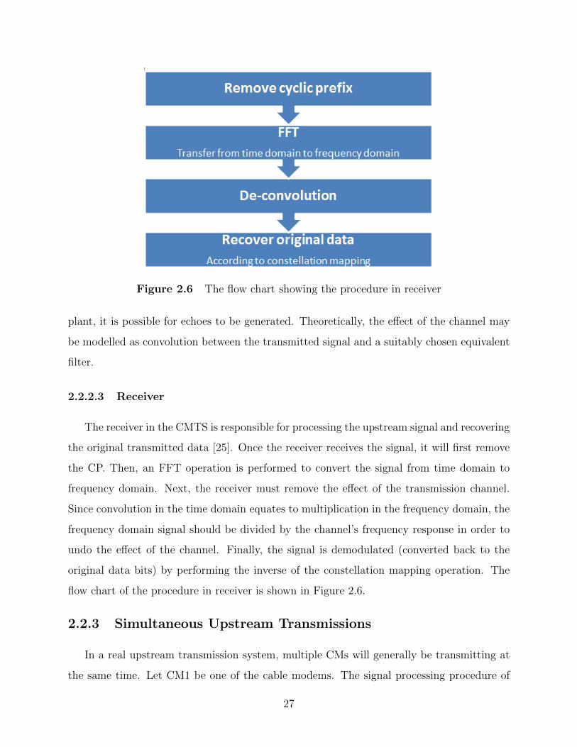
Figure 2.6 The flow chart showing the procedure in receiver
plant, it is possible for echoes to be generated. Theoretically, the effect of the channel may
be modelled as convolution between the transmitted signal and a suitably chosen equivalent
filter.
2.2.2.3 Receiver
The receiver in the CMTS is responsible for processing the upstream signal and recovering
the original transmitted data [25]. Once the receiver receives the signal, it will first remove
the CP. Then, an FFT operation is performed to convert the signal from time domain to
frequency domain. Next, the receiver must remove the effect of the transmission channel.
Since convolution in the time domain equates to multiplication in the frequency domain, the
frequency domain signal should be divided by the channel’s frequency response in order to
undo the effect of the channel. Finally, the signal is demodulated (converted back to the
original data bits) by performing the inverse of the constellation mapping operation. The
flow chart of the procedure in receiver is shown in Figure 2.6.
2.2.3 Simultaneous Upstream Transmissions
In a real upstream transmission system, multiple CMs will generally be transmitting at
the same time. Let CM1 be one of the cable modems. The signal processing procedure of
27

Figure 2.7 The basic signal processing progress of one CM
Figure 2.8 The signal produced by one CM
CM1 is studied as an example in this section. Figure 2.7 shows the basic progress used by
CM1 when processing and packaging data.
The original data is an array of digital bits. Take 0 1 1 0 0 0 1 1 for an example. According
to the chosen constellation type, the original data is transferred to decimal values. For
example, assuming QPSK is chosen for CM1 (M=4), then the binary data can be rearranged
into 2-bit chunks. The possible values for these 2-bit chunks are 01, 10, 00, 11, which are
1 2 0 3 in decimal. These numbers are then mapped to symbols according to the QPSK
constellation map. After mapping, the data will be allocated to the assigned sub-carriers.
Assume CM1 is assigned to the first minislot (sub-carrier 74 to 81). All other CMs are
assigned to other minislots. For example, CM5 could be assigned to minislots containing
sub-carriers 90-105. Each CM transmits on only the minislots assigned to it, leaving the
other sub-carriers empty. The transmitted signal from the CM is generated by applying an
IFFT and then adding a cyclic prefix and windowing the signal as previously discussed.
The signal generated by one CM is shown in Figure 2.8 . The data sent out by a cable
modem in time domain is called OFDM Data Block in the figure.
The structure of the upstream communication system was shown in Figure 2.4. The
28

Figure 2.9 The structure of signal sent out by upstream transmitters
signal transmitted through the channel is the sum of all cyclic prefix and data blocks sent
out by all CMs. As Figure 2.9 shows, the data blocks from multiple CMs combine to form
a single OFDM symbol. Note that transmitters are synchronized, so their data blocks and
cyclic prefixes line up in time.
When the CMTS receives the transmitted signal, it will first remove the cyclic prefix
part. Then the demodulator will capture and demodulate one symbol at a time in sequence.
If there is no noise, and no interference, the demodulator will recover all the data sent by all
CMs. In this example, the output of FFT for the sub-carriers 74 to 81 will be exactly the
same as the input of IFFT in CM1. The output of sub-carriers 90 to 105 will be the same
as the input of CM5.
29

3. Chapter3: Effects of Interference on a Single
Sub-carrier
In a practical setting, interference will be introduced into the transmission system. Two
main sources of interferences are considered in this thesis. One is the neighbouring symbols
and the other is self inflicted from the symbol of interest. The two sources of interferences are
referred to as the Inter Symbol Interference (ISI) and the Intra Symbol Interference (IaSI),
respectively. Both have been alluded to in Chapter 1, Section 1.3.4.
The upstream signal is transmitted as a frame consisting of K OFDMA symbols separated
by cyclic prefixes as illustrated in Figure 3.1. The received signal differs from the transmitted
signal in that it contains an echo as shown in Figure 3.2. The echo is shown below the main
path and is the main path scaled in amplitude and delayed by D.
It is assumed a synchronization circuit finds the boundaries of the OFDMA symbols in
the main path. Many such circuits [26] [27] and devices [28] have been discussed in the
literature over the years. These boundaries are shown in Figure 3.2 as red vertical dashed
lines. The demodulation of each symbol begins with the receiver extracting the portion of
the received signal within these boundaries. The extracted signal is the sum of the OFDMA
symbol in the main path plus the portion of the echo that falls in the extraction interval as
Figure 3.1 The transmitted signal in a frame consisting of K OFDMA symbols
30

Figure 3.2 The received signal (The upper plot is the main path; the lower plot is
an echo with delay D, where D is shorter than the length of CP)
Figure 3.3 The received signal (The upper plot is the main path; the lower plot is
an echo with delay D, where D is longer than the length of CP)
shown in Figure 3.2.
Whether or not there is interference depends on whether the length of the cyclic prefix
is longer than the echo’s delay. If the echo’s delay is shorter than the length of the cyclic
prefix, which is the case illustrated in Figure 3.2, the echo, which starts at the beginning of
CP, starts prior to the extraction interval and finishes after the extraction interval. Thus,
the echo spans the extraction interval. However, if the delay is longer than the cyclic prefix,
which is illustrated in Figure 3.3 , the echo does not start prior to the beginning of the
extraction interval, so it does not span the entirety of the extraction interval.
In the first case (Figure 3.2), the transmitter’s pre-equalizer can remove the effect caused
by the echo and the demodulator is able to recover the original signal perfectly. However, in
the second case, the pre-equalizer cannot compensate for the missing segment of the echo.
31

For the second case (Figure 3.3), a piece of the echo is missing from the extracted portion
of the signal. Since the signal is the sum of the main path and the echo, this missing piece for
all intents and purposes, is interference. Since this interference is self inflicted, it is referred
to as Intra Symbol Interference (IaSI). The symbol ’IaSI’ is used to refer to the power in
the self inflicted interference.
Furthermore, in the second case (Figure 3.3), a portion of the echo of the previous
symbol has shifted into the extraction interval. This unwanted signal is also a source of
interference. As this interference is inflicted by another symbol, it is referred to as Inter
Symbol Interference (ISI). The symbol ‘ISI’ is used to refer to the power in the Inter
Symbol Interference. The total interference power is the sum of IaSI and ISI and is
denoted ISITOTAL, where
ISITOTAL = IaSI + ISI; (3.1)
A more detailed explanation of ISI and IaSI is given in Section 3.1.2.
IaSI and ISI are the powers of the interference corrupting the entire OFDMA symbol.
Also of interest are the components of ISI and IaSI that corrupting a single sub-carrier, say
sub-carrier K. The component of ISI corrupt sub-carrier K is denoted ISISC(K). The
component of IaSI corrupting sub-carrier K is denoted IaSISC(K).
The components of ISI and IaSI corrupting sub-carrier K may not be the same as
the components of ISI and IaSI generated by sub-carrier K. Therefore, the components
generated by sub-carrier K are denoted ISISC(K) and IaSISC(K).
The intent of this chapter is to determine how ISISC(K) and IaSISC(K) is distributed
among ISISC(i) and IaSISC(i) for i = 1, 2, . . . , 2048 and also to determine what is the
total interference in ISITOTAL(i) is for i = 74, 75, . . . , 1973.
The system used for the analysis has only one active sub-carrier, which is SC-74. This
sub-carrier is QPSK modulated with random data. The channel has an echo with magnitude
-16dB with respect to the main path. The echo has a delay D = 500 samples, while the CP
has length 256. Since the echo’s delay is longer than the CP, both ISI and IaSI will be
present.
32

In Section 3.1, this system is analysed to compute the portion of the adjacent symbol’s
echo that causes ISI and missing portion of the self echo IaSI. Then, the distributions of
ISISC(74), IaSISC(74) and the ISITOTAL(74) across sub-carriers 1 to 2048, (i.e. ISISC(i),
IaSISC(i), ISITOTAL(i) for i = 1, 2, . . . , 2048) are plotted.
The results of Section 3.1 were obtained from a less than rigorous analysis. To corroborate
the ISI and IaSI obtained in Section 3.1, Section 3.2 provides a second method of computing
the distribution of the total interference in the system. The transmission model used is
the same as that in Section 3.1. This method computes and compares the constellation
points constructed in the receiver to the expected. The Euclidean distance between the
reconstructed and expected constellation points is the magnitude of error. The total power
in the interference is the sum of the square of the magnitude of the error. The distribution
of the total interference is plotted. By carefully comparing the plot generated in Section 3.1
and the plot generated in this section, the ISI and IaSI obtained in Section 3.1 can be
corroborated.
Section 3.3 includes an estimation model. A mathematical method is used to achieve the
same distributions of ISI, IaSI and ISITOTAL as the plots generated in Section 3.1. The
corroborated ISI and IaSI in Section 3.1 is applied to this model.
The ISISC(K) and IaSISC(K) generated by a single sub-carrier K is able to be estimated
by the estimation model built in Section 3.3. In Section 3.4, the transmission model used is
the same as the one built in Section 3.1. However, instead of having only one sub-carrier,
more sub-carriers are enabled and the signal is transmitted with different delay lengths.
Then, in the system, more sub-carriers have ISI and IaSI. For sub-carrier SC-i, ISISC(i)
should be the sum of all ISI generated by all other sub-carriers and IaSISC(i) should be the
sum of all IaSI generated by other sub-carriers. The total interference corrupting in SC-i is
the sum of ISISC(i) and IaSISC(i). This will be applied to the next chapter for final cyclic
prefix length selection model.
33

Figure 3.4 The impulse response of the physical channel linking a CM to the
CMTS
3.1 The Distribution of the Interference Generated by a Single
Sub-carrier
In this section, the distribution of the interference generated by a single sub-carrier among
all other sub-carriers is studied. To be more specific, the effects of the interference generated
by sub-carrier K, which has component ISISC(K), IaSISC(K) and ISITOTAL(K), on the
other sub-carriers are studied. The interference is generated and its distribution is measured
using time-domain simulation. Then, the so found distributions of ISISC(K), IaSISC(K)
and ISITOTAL(K) are plotted. Finally, the effects of the echo’s delay, the echo’s magnitude,
the length of the cyclic prefix and the modulation order are explored.
3.1.1 Channel Model for Physical Plant
The channel is modelled as a main path and an echo [29]. The impulse response of such
a channel is shown in Figure 3.4. This channel is expressed mathematically as:
hC(t) = Amδ(t− τm) + Aeδ(t− τm − τe); (3.2)
where τm is the transport delay of the main path and τe is the excess delay of the echo, which
will be referred to as the echo’s delay. Am is the magnitude of the main path and Ae is the
magnitude of the echo. A block diagram of this channel model is shown in Figure 3.5. The
block diagram in Figure 3.5 indicates the main path signal is received a time of τm after it
is transmitted. The echo is received τe after the main path is received.
The delay τm and amplitude Am are compensated by the synchronization circuit in the
34

Figure 3.5 The block diagram of the physical channel linking a CM to the CMTS
Figure 3.6 The block diagram of the physical channel used in this study (amplitude
and delay of the main path compensated)
receiver [30] and therefore have no effect on the performance of the system. Therefore,
without loss of generality, τm can be set to 0 and Am can be set to 1. This is done to obtain
the channel model used in this study, which is shown in Figure 3.6.
3.1.2 Sources of Interference
The interference of interest in this section is that generated when only one sub-carrier in
the OFDMA symbol has non-zero power. This active sub-carrier is denoted as Sub-carrier
K. An OFDMA symbol with only one active sub-carrier is a pure sinusoid, as shown in
Figure 3.7.
This OFDMA symbol is extended by copying a portion from the end of the symbol and
inserting it at the beginning as shown in Figure 3.8. The piece inserted at the beginning,
which is called a Cyclic Prefix (CP), will be a natural extrapolation of the sinusoid because
the period of the sinusoid is the length of the OFDMA symbol [31].
35

Figure 3.7 The sinusoid in one OFDMA symbol
Figure 3.8 The OFDMA symbol with cyclic prefix
36

Figure 3.9 The received signal which is the sum of the main path and an echo
(The echo’s delay shorter than the length of CP)
The transmitted signal traverses the channel shown in Figure 3.6 and arrives at the
receiver with an echo. The received signal is illustrated in Figure 3.9. In this case, the
channel is such that the echo’s delay is shorter than the length of the cyclic prefix.
The receiver is synchronized to extract the received signal in the interval between the
two vertical dashed lines in Figure 3.9. This interval, which is referred to as the extraction
interval, is aligned with the OFDMA symbol in the main path.
If the echo’s delay is longer than the length of the cyclic prefix, which is illustrated in
Figure 3.10, the echo in the extraction interval is no longer a complete sinusoid. Conceptually,
the sinusoid can be completed as shown in Figure 3.11, in which two segments are added
to the section of the extraction interval between lines L1 and L2. One segment is chosen to
complete the sinusoid and the other is chosen to make the two segments sum to 0. The black
curve between lines L3 and L4 is the portion of the echo that originated from the original
OFDMA symbol. The red curve between lines L2 and L3 originated from the cyclic prefix.
37

Figure 3.10 The received signal which is the sum of the main path and an echo
(The echo’s delay longer than the length of CP)
Figure 3.11 The echo in the extraction interval been completed by adding a segment
38

Figure 3.12 The diagram of the main path signal and an echo with delay D longer
than CP length
The lower green segment between lines L1 and L2 is not part of the echo and therefore is
not actually present in the real system. It is drawn to complete the sinusoid. To compensate
for the presence of this segment, the upper cyan segment between L1 and L2 is also added.
Since the upper and lower segments sum to zero, nothing has been added. This allows the
echo to be represented as a complete sinusoid plus interference, with the interference being
the upper cyan curve between lines L1 and L2. The power in this interference is denoted
as IaSI, which is short for Intra Symbol Interference. The echo’s delay in unit of samples
is denoted D. The length of the IaSI segment is the distance between L1 and L2, which in
units of samples is D minus the length of the CP in samples.
In the case where the echo’s delay is longer than the length of CP, the echo from the
previous symbol enters the extraction interval as shown in Figure 3.12. As Figure 3.12
shows, since the delay is longer than the CP length, part of the previous symbol will fall
into the extraction interval. This is illustrated in Figure 3.13 , where the dotted magenta
curve between lines L1 and L2 is the portion of the previous symbol’s echo that is shifted
into the extraction interval. Obviously, this portion of the previous symbol’s echo acts as
interference. The power in this interference is denoted as ISI, which is short for Inter Symbol
Interference. The length of the ISI segment is the distance between L1 and L2, which in
units of samples is D minus the length of the CP in samples.
Therefore, two kinds of interference corrupt the extraction interval: IaSI, which comes
from the incomplete self echo, and ISI, which comes from the echo of the previous symbol.
39

Figure 3.13 The echo in the extraction interval been completed by adding a segment
and include the previous symbol’s echo
Both types of interference segments have lengths of D minus CP samples.
The inter symbol interference power is given by the following equation which is taken
from the DOCSIS 3.1 standard.
ISI =(τe − TCP )A2
e
TU; (3.3)
where:
τe is the delay of the echo
TCP is the length of cyclic prefix in µs
Ae is the amplitude of the echo with respect to amplitude of the main path
TU is the duration of the extraction interval in seconds, which is also FFT duration (20 or
40 µs)
The length of the cyclic prefix in unit samples is denoted NCP . The relationship between
the length of the cyclic prefix, the delay and the ISI (power) in unit of samples is given by:
ISI =(D −NCP )A2
e
NFFT
; (3.4)
Using the same approach, an equation for IaSI (power) can be derived with the result:
IaSI =(τe − TCP )A2
e
TU; (3.5)
40

where:
τe is the delay of the echo which is caused by a micro-reflection
TCP is the length of cyclic prefix in µs
Ae is the amplitude of the micro-reflection with respect to amplitude of the main path
TU is the duration of the extraction interval in seconds, which is also FFT duration (20 or
40 µs)
The relationship between the length of the cyclic prefix, the delay and the IaSI (power)
in unit of samples is given by:
IaSI =(D −NCP )A2
e
NFFT
; (3.6)
From (3.4) and (3.6), it is clear that ISI equals IaSI. The reason for this is clear from
Figure 3.13 that shows the length of the IaSI segment is the same as the length of ISI
segment. Since the previous symbol traverses the same channel, it has the same delay and
echo strength. This means the average power of the IaSI segment is equal to the average
power of the ISI segment. The total interference power is the sum of IaSI and ISI, i.e.
ISITOTAL = ISI + IaSI; (3.7)
Since ISI = IaSI; ISITOTAL = 2× ISI; which has
ISITOTAL = 2× (τe − TCP )A2e
TU; (3.8)
where:
τe is the delay of the echo which is caused by a micro-reflection
TCP is the length of cyclic prefix in µs
Ae is the amplitude of the echo with respect to amplitude of the main path
TU is the duration of the extraction interval in seconds, which is also FFT duration (20 or
40 µs)
The ISITOTAL is related to the echo’s delay, the echo’s strength, the length of the cyclic
prefix and the length of the OFDMA symbol in unit of samples by:
ISITOTAL = 2× (D −NCP )A2e
NFFT
; (3.9)
41

Table 3.1 The parameters for the OFDM system used in the simulation
Length of the OFDMA symbol NFFT 2048
Enabled Sub-carrier SC-74
Modulation Type QPSK
Length of Cyclic Prefix NCP 256
Length of Roll-off Period NRP 0
Echo’s Delay Length D 500
Echo’s Magnitude Ae -16dB
3.1.3 Calculation of the Distribution of ISISC(K) and ˜IaSISC(K)
Having identified the sources of ISI and IaSI in the system, the distribution of the
interferences generated by an OFDMA symbol with a single non-zero sub-carrier can be
computed. The approach taken is to use Fourier analysis on the segment of the echo causing
the ISI to translate it from the time domain to the frequency domain. Once in the frequency
domain the distribution of power across sub-carriers is easily computed. Since the nature of
IaSI parallels that of ISI and IaSI is equal to ISI, only one type of interference needs to
be analyzed in this way.
The analysis is done using a MATLAB simulation with the MATLAB function FFT
being used to transform the echo segment causing the ISI into the frequency domain. The
OFDM system model introduced in Section 2.2.2 is in a MATLAB script. Random data
is generated and assigned to OFDMA symbols with cyclic prefixes in the MATLAB script
“OFDM Tx”. The channel, which has a main path and an echo, is constructed in MATLAB
script ”Channel”. It is pointed out that the white Gaussian noise that is normally introduced
in the channel is not modelled here.
The OFDM system is configurable through a set of parameters. The parameters for the
OFDM system used in the simulation are set as shown in Table 3.1. For the purpose of this
study, the non-zero sub-carrier is Sub-carrier 74.
A frame consists of K consecutive symbols. However, only two of the K symbols in this
42

Figure 3.14 The structure of the transmitted signal
Figure 3.15 The received signal with one main path and an echo with delay D and
magnitude Ae
sequence needs to be generated in the simulation. The structure of the signal generated
in the MATLAB simulation is shown in Figure 3.14. As explained earlier, each of the two
symbols have the same non-zero sub-carrier, which is Sub-carrier 74. The sub-carrier in the
two symbols is modulated with independent data.
The main path in the channel is modelled with no delay and a gain of 1. The echo is
modelled with a delay of D samples and a gain Ae. This channel, which is the sum of the
main path and the echo is constructed in MATLAB as a filter with coefficients [1, 0, 0...,
0, Ae], where D − 1 zeros separate the first and last coefficients. The first coefficient is the
gain of the main path, which is 1, and the last coefficient is the gain of the echo, which is
Ae. The received signal is constructed by convolving the transmitted signal with the filter
that models the channel.
At the receiver, the received signal contains a main path and an echo as illustrated in
Figure 3.15. Of interest is the case where D is longer than NCP . In this case the portion
of the echo from the previous symbol is shifted in the extraction interval and causes inter
symbol interference.
The case of interest is demonstrated in Figure 3.16, where the echo for OFDMA Symbol
1 reaches the extraction interval for Symbol 2. The extraction interval for OFDMA Symbol
43

Figure 3.16 The received main path and the echo scaled in unit of samples
2 is highlighted in red and the portion in the echo of the OFDMA Symbol 1 that reaches the
extraction interval has been hatched. Figure 3.16 starts with the first sample of OFDMA
Symbol 1, and ends with the last sample of the echo for Symbol 2. The segment that causes
ISI starts at sample 2×NCP +NFFT and ends at sample D+NCP +NFFT . Therefore, the
interference segment of the echo can be obtained by subtracting the segment of the main
path for OFDMA Symbol 2, that starts at sample 2 × NCP + NFFT and ends at sample
D +NCP +NFFT , from the received signal .
The next step is to take the Fast Fourier Transform of the segment causing the interfer-
ence. This is done by extending this segment with zeros to make its length NFFT . Then,
in the frequency domain, the power of this segment is computed. The computed power
distribution is the ISI distribution generated by Sub-carrier 74, which is referred to as
ISISC(74).
While the computation discussed here was done for Sub-carrier 74, the technique can be
applied to any active sub-carriers. The MATLAB code used for this analysis is included in
Appendix B.
3.1.4 Result
The ISI and IaSI distribution over the whole frequency domain can be plotted using
the technique developed in Section 3.1.3.
With all the parameters set as shown in Table 3.1, the ISI is distributed as illustrated
44

Figure 3.17 ISI distribution with NCP =256, echo delay D=500, echo magnitude
Ae = −16dB and the only non-zero sub-carrier SC-74
in Figure 3.17.
The x-axis of Figure 3.17 is the frequency expressed as sub-carrier number, which starts
at 1 and goes to 2048. The y-axis is ISI shown in dB, i.e. 10 log(ISI/ReferencePower)1.
The vertical red dashed line marks the Sub-carrier 74. The plot shows the interference power
generated by Sub-carrier 74 is concentrated in the vicinity of that sub-carrier, but does reach
all sub-carriers. The interference on Sub-carrier K is a strong function of its distance from
Sub-carrier 74. The distribution is circular in the sense that the power in Sub-carrier 74+K
1The reference power chosen for expressing ISI in dB is the average power of the received symbol after
subtracting the interference. The received signal is the sum of the main path and the echo. Should a piece of
the echo be missing from the extraction interval. The missing piece is replaced for the purpose of calculating
the signal power.
In terms of the constellation, the reference power is the average power of the received constellation in
absence of noise and interference. This received constellation includes the effect of the echo, which will scale
its magnitude and rotate it.
45

Figure 3.18 IaSI distribution with NCP =256, echo delay D=500, echo magnitude
Ae = −16dB and the only non-zero sub-carrier SC-74
is equal to the power in Sub-carrier modulo(2048, 74−K).
The IaSI distribution is shown in Figure 3.18 . It is identical to the distribution of ISI.
The distribution of the total interference power, is calculated in similar fashion and is shown
in Figure 3.19.
3.1.5 Effect of Parameter Values
The factors that affect the distribution of interference are explored in this section. The
effect of changing the length of cyclic prefix, the echo’s delay, the echo’s magnitude as well
as the constellation order are determined by changing one parameter at a time.
3.1.5.1 The Effect of the Length of Cyclic Prefix on ISI
To determine the effect of the length of the cyclic prefix, NCP is changed from 256 to
96 samples. The other parameters remain unchanged, i.e. the echo’s delay D equals 500,
the echo’s magnitude Ae equals −16dB and the modulation type is QPSK. The spectral
46

Figure 3.19 ISITOTAL distribution with NCP =256, echo delay D=500, echo mag-
nitude Ae = −16dB and the only non-zero sub-carrier SC-74
47

Figure 3.20 ISI distributions comparison between the length of the cyclic prefix
NCP = 96 and 256
distribution of the ISI is plotted in Figure 3.20 with a solid line that is magenta in color.
The plot on the right side is a zoomed-in view of the plot on the left side. The dashed blue
curve is the ISI distribution plotted in Figure 3.17, in Section 3.1.4 for the length of cyclic
prefix NCP = 256. The solid magenta curve is the ISI distribution with the length of the
cyclic prefix being 96.
It can be seen from the zoomed-in plot in Figure 3.20, that the ISI at SC-74 for NCP =
256 is about 4dB less than the ISI for NCP = 96. The difference in the ISI at the other
sub-carriers decreases with the distance from Sub-carrier 74.
The shorter CP length produces larger ISI in the vicinity of sub-carrier generating the
interference, which is Sub-carrier 74. The reason is straight forward. For the shorter length
of the cyclic prefix, a larger portion of the previous symbol’s echo shifts into the extraction
interval, thus increasing the interference. In fact, this is the rationale for the development
of equation (3.4).
48

Figure 3.21 ISI distributions comparison between the echo’s delay D= 500 and
1000
3.1.5.2 The Effect of the Echo’s Delay on ISI
To determine the effect of the echo’s delay, it is changed from D = 500 to 1000 samples
and the length of the cyclic prefix is changed back to 256. All other parameters remain
unchanged, i.e. the echo’s magnitude Ae equals −16dB and the modulation type is QPSK.
The spectral distribution of the ISI is plotted in Figure 3.21 with a solid magenta line. The
plot on the right side is a zoomed-in view of the plot on the left side. Again, the dashed blue
curve is the ISI distribution plotted in Figure 3.17, in Section 3.1.4 for the echo’s delay D
= 500. The solid magenta curve is the ISI distribution with the D = 1000.
It can be seen from the zoomed-in plot in Figure 3.21 that the ISI at Sub-carrier 74 for
D = 500 is about 11dB less than the ISI for D = 1000. The difference in the ISI at other
sub-carrier decreases with the distance from Sub-carrier 74.
The echoes with longer delays produce larger ISI in the vicinity of the sub-carrier gen-
erating the interference, which is Sub-carrier 74. The reason is also straight forward. For
the echo with a longer delay, a larger portion of the previous symbol’s echo shifts into the
extraction interval, thus increasing the interference.
49

Figure 3.22 ISI distributions comparison between the echo’s magnitude Ae =
−16dB and −35dB
3.1.5.3 The Effect of the Echo’s Magnitude on ISI
To determine the effect of the echo’s magnitude, it is changed from Ae = −16dB to
−35dB and the echo’s delay is changed back to 500 samples. All other parameters remain
unchanged, i.e. the length of the cyclic prefix is 256 and the modulation type is QPSK.
The spectral distribution of the ISI is plotted in Figure 3.22 with a solid line in the color
of magenta. The plot on the right side is a zoomed-in view of the plot on the left side.
The dotted blue curve is the ISI distribution plotted in Figure 3.17, in Section 3.1.4 for an
echo with magnitude Ae = −16dB, which is measured relative to the main path. The solid
magenta curve is the ISI distribution with Ae = −35dB.
It can be seen from the zoomed-in plot in Figure 3.22 that at Sub-carrier 74, the ISI
caused by the echo with magnitude −16dB is −33.11dB. The ISI caused by the echo with
magnitude −35dB is −53.25dB. The ISI on all sub-carriers seems to be proportional to the
echo strength. The ISI distribution for the stronger echo of −16dB, is about 20dB higher
than the ISI distribution for the weaker echo of Ae=−35dB across the entire spectrum.
Of note, the change in ISI does not exactly track the change in Ae. The echo’s magnitude
50

Ae is changed by 19dB (from −16dB to −35dB), while the ISI is changed by 20.14dB. The
reason for the difference is explained below.
Mathematically, ISI expressed in dB is computed with (3.10).
ISIindB = 10 log10
ISI
Pref; (3.10)
where Pref is the reference power, which is the power in the sum of the main path and
the echo. Obviously, the reference power will depend on the amplitude of the echo. The
difference in between ISI in dB for Ae = −16dB and the ISI in dB for Ae = −35dB is
denoted ISIDIFF . It is given by
ISIDIFF = 10 log10
ISI16Pref16
− 10 log10
ISI35Pref35
; (3.11)
where ISI16 represents the ISI (power) for Ae = −16dB and ISI35 represents the ISI
(power) for Ae = −35dB. The reference powers for echoes’ magnitudes −16dB and −35dB
are denoted Pref16 and Pref35 respectively.
Equation ( 3.11) can be written as:
ISIDIFF = 10 log10(
ISI16Pref16ISI35Pref35
); (3.12)
ISIDIFF = 10 log10(ISI16ISI35Pref35Pref16
); (3.13)
which can be simplified to:
ISIDIFF = 10 log10 ISI16 − 10 log10 ISI35 + 10 log10 Pref35 − 10 log10 Pref16; (3.14)
ISIDIFF = 19dB + 10 log10 Pref35 − 10 log10 Pref16; (3.15)
Since ISIDIFF read from Figure 3.22 is 20dB,
10 log10 Pref35 − 10 log10 Pref16 = 1dB; (3.16)
This means the echo adds destructively to the main path.
51

Figure 3.23 ISI distributions comparison between QPSK and 16-QAM systems
3.1.5.4 The Effect of the Modulation Order on ISI
To determine the effect of the modulation order on the ISI, the modulation type is
changed from QPSK to 16-QAM and the echo’s magnitude Ae is changed back to −16dB.
All other parameters remain unchanged, i.e. the length of the cyclic prefix is 256, the echo’s
delay is 500 samples. The spectral distribution of the ISI is plotted in Figure 3.23 with a
solid line that is magenta in color. The plot on the right side is a zoomed-in view of the
plot on the left side. The dashed blue curve is the ISI distribution plotted in Figure 3.17,
in Section 3.1.4 for the constellation type of QPSK. The solid magenta curve is the ISI
distribution with the constellation type being QPSK.
It can be seen from the zoomed-in plot in Figure 3.23, that the distribution of ISI
across the entire frequency spectrum for QPSK is almost equal to the distribution of ISI
for 16-QAM. The ISI at Sub-carrier 74 for both QPSK and 16-QAM plot are about -34dB.
Therefore, the constellation order will not have a significant effect on the distribution of
ISI across the entire frequency spectrum.
52

3.1.6 Conclusion
From observations made in Section 3.1.5.1, Section 3.1.5.2, Section 3.1.5.3 and Sec-
tion 3.1.5.4, it can be concluded that the length of the cyclic prefix and the echo’s delay
affect the distribution of the ISI most severely at frequencies near the sub-carrier causing
the ISI. The echo’s magnitude affects the ISI across the entire frequency spectrum and is
nearly proportional to the echo’s strength. The constellation type doesn’t have a significant
effect on the ISI.
Since Intra Symbol Interference has the same characteristics and value as the Inter Symbol
Interference, its spectral distribution will be the same. Therefore, the total interference, i.e.
ISITOTAL, which is the sum of IaSI and ISI, will be twice that of ISI.
3.2 Corroboration of the Distribution of the Interference Gener-
ated by a Single Sub-carrier
In Section 3.1, the distribution of the interference generated by a single sub-carrier was
analyzed. In this section an independent simulation that is based on modelling the decision
variable, i.e. the constellation points constructed from the received signal with interference
removed is constructed for the purpose of corroborating the results of Section 3.1. The
corroboration is done by analyzing the constellation points constructed from the received
signal first to find the error caused by interference. The average power in the error is
computed and compared with the total ISI obtained from Section 3.1.
3.2.1 The Distribution of ISITOTAL(K)
The distribution of ISITOTAL(K) is found by modulating the sub-carriers using QPSK.
The constellation map for QPSK is illustrated in Figure 3.24. The four points, 1 + j, 1− j,
−1 + j, −1− j, (blue) are the constellation of the transmitted signal.
The channel consists of a main path and an echo. The echo doesn’t cause interference
if its delay is shorter than the length of the cyclic prefix. However, even without causing
interference, the echo will affect the constellation constructed from the received signal. The
53

Figure 3.24 The transmitted constellation of QPSK
echo can add constructively or destructively to the main path signal, causing the constellation
to scale up or down. In addition to scaling, depending on the phase of the echo with respect
to the main path signal, the echo can cause a rotation in the constellation. The amount of
rotation depends on the phase of the echo with respect to the main path signal.
The mathematical explanation is given below. Assume only one OFDMA symbol is
transmitted through the system and that the transmitted symbol is a single sub-carrier (i.e.
a single sinusoid) with amplitude 1. The transmitted signal for constellation point −1− j1
can be expressed as
Transmitted Signal = (−1− j1)ejω0t; (3.17)
where ω0 is the frequency of the single active sub-carrier.
Then, at the receiver the received signal should be
Received Signal = (−1− j1)ejω0t + Ae(−1− j1)ejω0(t−τ); (3.18)
where Ae is the echo’s magnitude and τ is the echo’s delay with respect to the main path.
54

Equation 3.18 can be rewritten as
Received Signal = (−1− j1)ejω0t + Aee−jω0τ (−1− j1)ejω0t
= (1 + Aee−jω0τ )(−1− j1)ejω0t
= Arxej(ω0t+θ); (3.19)
where the amplitude of the received signal Arx is given by
Arx =√
((1 + Aee−jω0τ )(−1− j1))2
=√
2√
1 + 2Ae cos(ω0τ) + A2e; (3.20)
and the expression of the phase shift θ is
θ = angle((1 + Aee−jω0τ )(−1− j1))
= angle(−(1 + Ae(sinω0τ + cosω0τ))− j1(1 + Ae(sinω0τ − cosω0τ)))
= tan−11 + Ae(sinω0τ − cosω0τ)
1 + Ae(sinω0τ + cosω0τ). (3.21)
The factor of√
2 in Equation 3.20 is the magnitude of the transmitted constellation
point, which is | − 1− j1|. For QPSK all transmitted constellation points have a magnitude
of√
2, so Arx does not depend on the constellation point transmitted.
The effect of the echo on the received constellation map is illustrated in Figure 3.25. The
triangles (green) mark the received constellation points in the absence of any noise or other
distortion. Clearly, it is a scaled and rotated version of the transmitted constellation. From
Figure 3.25, it can be seen that each point in the constellation is rotated by the same amount
θ. Since the constellation of Figure 3.25 has no noise or interference, it forms the reference
constellation for the receiver.
In the event that the echo’s delay is longer than the length of the cyclic prefix, interference
corrupts the reference constellation. This interference causes the decision variable to move
off the reference constellation. The effect of the interference on the sub-carrier that was
transmitted with an amplitude −1 − j1 (i.e. constellation point (−1, −1), is illustrated in
Figure 3.26. At the receiver, the demodulation produces a decision variable which is an
55

Figure 3.25 The transmitted constellation and the reference constellation of QPSK
Figure 3.26 The transmitted constellation, the reference constellation and the re-
ceived constellation of QPSK
56

estimation of the transmitted constellation point. The decision variable is represented by
the diamond mark (red). The interference causes the decision variable (the diamond) in the
receiver to deviate from the reference point (the triangle).
The magnitude and phase of the decision variables depend on which of the four constel-
lation points that was sent in the previous symbol. Only one of these four points is shown
in Figure 3.9. All constellation points will be affected in a similar fashion.
Since no noise has been added to the signal, the error in the decision variable is caused
entirely by ISI and IaSI. Then, the power in the total interference can be computed
by summing the power of the differences between the received decision variables and the
associated reference constellation points. For the purpose of expressing the total interference
in dB, the power used for the reference is chosen to be the average power of the reference
constellation.
Having identified the total interference power in the system, the distribution of the total
interference generated by an OFDMA symbol with a single non-zero sub-carrier can be
computed. The analysis is done using a MATLAB simulation by tracking the decision
variables for all of the OFDMA sub-carriers at the demodulator. Note that the expected
(reference) decision variable for the sub-carriers which had no transmitted data is 0. In other
words, any received decision variable on those sub-carriers is considered as interference. The
OFDM system model used in Section 3.1.3 was modified and then modeled in a MATLAB
script. Random data is generated and assigned to OFDMA symbols with cyclic prefixes in
the MATLAB script “OFDM Tx”. The channel, which has a main path and an echo, is
constructed in MATLAB script“Channel”. The demodulation that is done in the receiver is
constructed in MATLAB script “OFDM Rx”. (see Appendix C for a complete listing of the
Matlab code)
The OFDM system is configurable through a set of parameters. The parameters for the
OFDM system used in the simulation are set as shown in Table 3.2. For the purpose of this
study, the non-zero sub-carrier is Sub-carrier 74.
As in Section 3.1.3, only two OFDMA symbols are constructed in the simulation. As
57
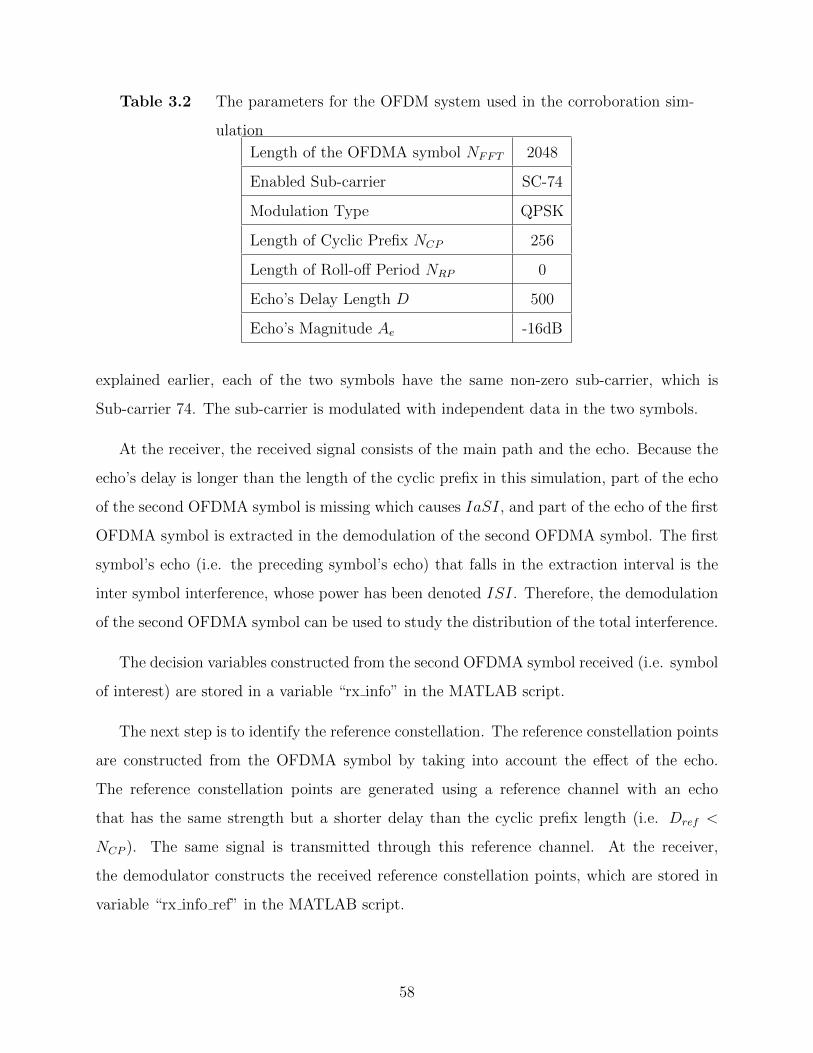
Table 3.2 The parameters for the OFDM system used in the corroboration sim-
ulation
Length of the OFDMA symbol NFFT 2048
Enabled Sub-carrier SC-74
Modulation Type QPSK
Length of Cyclic Prefix NCP 256
Length of Roll-off Period NRP 0
Echo’s Delay Length D 500
Echo’s Magnitude Ae -16dB
explained earlier, each of the two symbols have the same non-zero sub-carrier, which is
Sub-carrier 74. The sub-carrier is modulated with independent data in the two symbols.
At the receiver, the received signal consists of the main path and the echo. Because the
echo’s delay is longer than the length of the cyclic prefix in this simulation, part of the echo
of the second OFDMA symbol is missing which causes IaSI, and part of the echo of the first
OFDMA symbol is extracted in the demodulation of the second OFDMA symbol. The first
symbol’s echo (i.e. the preceding symbol’s echo) that falls in the extraction interval is the
inter symbol interference, whose power has been denoted ISI. Therefore, the demodulation
of the second OFDMA symbol can be used to study the distribution of the total interference.
The decision variables constructed from the second OFDMA symbol received (i.e. symbol
of interest) are stored in a variable “rx info” in the MATLAB script.
The next step is to identify the reference constellation. The reference constellation points
are constructed from the OFDMA symbol by taking into account the effect of the echo.
The reference constellation points are generated using a reference channel with an echo
that has the same strength but a shorter delay than the cyclic prefix length (i.e. Dref <
NCP ). The same signal is transmitted through this reference channel. At the receiver,
the demodulator constructs the received reference constellation points, which are stored in
variable “rx info ref” in the MATLAB script.
58

Therefore, the total interference power of Sub-carrier 74 can be computed with:
ISITOTAL(74) =
Numof ConstellationPoints∑i=1
|rx−info(i)− rx−info−ref(i)|2 (3.22)
In units of dB, the total interference is given by:
ISITOTAL(74)(dB) = 10 log10
ISITOTAL(74)
Reference−Power(3.23)
where the reference power at the denominator is the total power of the received reference
constellation points.
Reference−Power =
Numof ConstellationPoints∑i=1
|rx−info−ref(i)|2; (3.24)
The main MATLAB script of the simulation is included in Appendix C.
3.2.2 Result
The ISITOTAL distribution over the whole frequency domain can be plotted using the
corroboration model developed in Section 3.2.1. It is compared with the distribution of the
total interference obtained from the simulation model introduced in Section 3.1.
All parameters are set as they were for the simulation in Section 3.1. These parameters
are shown in Table 3.3. The distribution of the total interference generated by a single
non-zero sub-carrier, SC-74, is illustrated in Figure 3.27. The x-axis of Figure 3.27 is the
frequency expressed as sub-carrier number, which starts at 1 and ends at 2048. The y-axis
is ISITOTAL in dB. The vertical dashed line (red) marks position of the Sub-carrier 74. The
solid curve (magenta) represents the distribution of ISITOTAL generated by the simulation
model of Section 3.1. The dashed curve (blue) is the distribution of ISITOTAL from the
simulation model of Section 3.2, which was constructed to the corroborate the model of
Section 3.1. The plot on the right side is a zoomed-in view Sub-carrier 74.
It can be seen from the zoomed-in plot in Figure 3.27, that the distribution of ISITOTAL
across the entire frequency spectrum from the model of this section is almost equal to the
distribution of ISITOTAL from the model of Section 3.1. The power distributions in the
vicinity of Sub-carrier 74 also match very well.
59

Figure 3.27 Distribution of ISITOTAL comparing the results of simulation model to
corroboration model for NCP=256, echo’s delay D=500, Echo’s mag-
nitude Ae = −16dB, QPSK modulation type and a single non-zero
sub-carrier, SC-74.
Left: Full frequency range
Right: Zoomed on Sub-carrier 74
Table 3.3 The parameters set for the OFDM system in the corroboration model
Length of the OFDMA symbol NFFT 2048
Enabled Sub-carrier SC-74
Modulation Type QPSK
Length of Cyclic Prefix NCP 256
Length of Roll-off Period NRP 0
Echo’s Delay Length D 500
Echo’s Magnitude Ae -16dB
60

Figure 3.28 Distribution of ISITOTAL comparing the results of simulation model
to corroboration model for NCP=96, echo’s delay D=500, Echo’s mag-
nitude Ae = −16dB, QPSK modulation type and a single non-zero
sub-carrier, SC-74.
3.2.3 Effect of Parameter Values
In Section 3.1.5, the effects of changing the length of cyclic prefix, the echo’s delay, the
echo’s magnitude as well as the constellation order on the distribution of ISI are explored.
To corroborate the effects of these factors concluded in Section 3.1.5 are right, in this section
the effects of these factors on ISITOTAL are determined by changing one parameter at a time.
3.2.3.1 Effect of the Length of Cyclic Prefix
The effect of the length of the cyclic prefix on the ISITOTAL is determined using the
model of this section by changing NCP from 256 to 96 samples. The other parameters remain
unchanged, i.e. the echo’s delay D equals 500, the echo’s magnitude Ae equals −16dB and
the modulation type is QPSK. The spectral distributions of the ISITOTAL generated by the
simulation model of Section 3.1 and 3.2 are plotted in Figure 3.28.
The solid curve (magenta) represents the distribution of ISITOTAL computed from the
simulation model in Section 3.1. The dashed curve (blue) is the distribution of ISITOTAL
61

generated by the constellation simulation model of this section. The plot on the right side
is a zoomed-in view of Sub-carrier 74.
It can be seen from the zoomed-in plot in Figure 3.28, that the curve generated from the
simulation of this section agrees very well with the curve generated in Section 3.1 when the
length of the cyclic prefix has length 96. Therefore, it can be concluded that model works
well for the cyclic prefixes of difference lengths.
3.2.3.2 Effect of the Echo’s Delay
The effect of the echo’s delay, was determined through simulation in Section 3.1. That
effect is corroborated here by computing the distribution of ISITOTAL using the constellation
based simulation method of this section. The echo’s delay D is changed from 500 to 1000
samples and the length of the cyclic prefix is changed back to 256 as they were in Section 3.1.
All other parameters remain unchanged, i.e. the echo’s magnitude Ae equals −16dB and
the modulation type is QPSK. The spectral distributions of the ISITOTAL generated by the
simulation model of Section 3.1 and the constellation based simulation in this section are
plotted in Figure 3.29.
The solid curve (magenta) represents the distribution of ISITOTAL generated by the
simulation model of Section 3.1. The dashed curve (blue) is the distribution of ISITOTAL
generated by the constellation based simulation. The plot on the right side is a zoomed-in
view of Sub-carrier 74.
It can be seen from the zoomed-in plot in Figure 3.29, that with the change of the echo’s
delay, the distribution of ISITOTAL across the entire frequency spectrum from the simulation
model fits the distribution of ISITOTAL from the corroboration model very well. Therefore,
it can be concluded that both models are accurate over a range of delays.
3.2.3.3 Effect of the Echo’s Magnitude
The constellation based simulation is used to corroborate the accuracy of the simulation
model of Section 3.1, when the echo’s magnitude Ae is changed from −16dB to −35dB and
62

Figure 3.29 Distribution of ISITOTAL comparing the results of simulation model
to corroboration model for NCP=256, echo’s delay D=1000, Echo’s
magnitude Ae = −16dB, QPSK modulation type and a single non-zero
sub-carrier, SC-74.
the echo’s delay is changed back to 500 samples. All other parameters remain unchanged,
i.e. the length of the cyclic prefix is 256 and the modulation type is QPSK. The spectral
distributions of the ISITOTAL generated by the simulation model of Section 3.1 and the
constellation based simulation in this section are plotted in Figure 3.30.
The solid curve (magenta) represents the distribution of ISITOTAL generated by the
simulation model in Section 3.1. The dashed curve (blue) is the distribution of ISITOTAL
generated by the constellation based simulation. The plot on the right side is a zoomed-in
view of the plot on the left side.
It can be seen from the zoomed-in plot in Figure 3.30, that with the change of the echo’s
magnitude, the distributions of ISITOTAL across the entire frequency spectrum from the
simulation model in Section 3.1 is almost equal to the distribution of ISITOTAL from the
constellation based simulation. Therefore, it can be concluded that both models are accurate
over a range of echo strengths.
63

Figure 3.30 Distribution of ISITOTAL comparing the results of simulation model to
corroboration model for NCP=256, echo’s delay D=500, Echo’s mag-
nitude Ae = −35dB, QPSK modulation type and a single non-zero
sub-carrier, SC-74.
3.2.3.4 Effect of the Modulation Order
The constellation based simulation is used to corroborate the accuracy of the simulation
model of Section 3.1 when the modulation type is changed from QPSK to 16-QAM. The
echo’s magnitude Ae is changed back to −16dB. All other parameters remain unchanged,
i.e. the length of the cyclic prefix is 256, the echo’s delay is 500 samples. The spectral
distributions of the ISITOTAL generated by the simulation model in Section 3.1 and the
constellation based simulation are plotted in Figure 3.31.
The solid curve (magenta) represents the distribution of ISITOTAL is generated by the
simulation model in Section 3.1. The dashed curve (blue) is the distribution of ISITOTAL
generated by the constellation based simulation in this section. The plot on the right side is
a zoomed-in view of Sub-carrier 74.
It can be seen from the zoomed-in plot in Figure 3.31, that with the change of the
constellation types, the distributions of ISITOTAL across the entire frequency spectrum from
64

Figure 3.31 Distribution of ISITOTAL comparing the results of simulation model to
corroboration model for NCP=256, echo’s delay D=500, Echo’s mag-
nitude Ae = −16dB, 16-QAM modulation type and a single non-zero
sub-carrier, SC-74.
the simulation model of Section 3.1 is almost equal to the distribution of ISITOTAL from the
constellation based simulation. Therefore, it can be concluded that both models are accurate
over a range of constellation orders.
3.2.4 Conclusion
From observations made in Section 3.2.3.1, Section 3.2.3.2, Section 3.2.3.3 and Sec-
tion 3.2.3.4, where comparisons between the simulation model in Section 3.1 and the con-
stellation based simulation in this section are made, it can be concluded that the two models
agree over a wide range of parameter values.
Therefore, the analysis of the effects of various parameters on the interference in the
system presented in Section 3.1 has been corroborated. The identified and corroborated
interference sources will be be included in the ISI estimation model in the next section.
65

3.3 Convolution Model for the Interference
The distribution of the interference generated by a single sub-carrier was analyzed in
Section 3.1 and corroborated in Section 3.2. In this section, yet another model is developed
and is analyzed to obtain estimates of the distribution of the interference generated by a single
sub-carrier. This model differs from the two previous models in that it is mathematically-
based rather than simulation-based. The goal is to develop an equation or set of equations
which can be used to predict the amount and distribution of interference in a system, given
estimates of the echo delay and strength. The model developed in this section involves the
convolution of the DFT of a symbol with the DFT of a mask and so it is referred to as the
convolution model.
The model is then used to find the aggregate interference on any one sub-carrier when all
the sub-carriers are “on”. The aggregate interference in simply the sum of the interferences
from all the “on” sub-carriers.
As explained in Section3.1.2, the nature of IaSI parallels that of ISI so only one type
of the interferences needs to be analyzed. It is ISI that is studied in this Section. The
principles that underpin the “convolution” model are explained in Section 3.3.1.
Again, the accuracy of the model developed in this section is corroborated by computing
the results to those obtained with the models developed in Section 3.1 and Section 3.2.
3.3.1 Convolution Based Model
As before, the channel considered in this section consists of a main path and an echo.
The case of interest here is where the echo’s delay is longer than the length of cyclic prefix, as
illustrated in Figure 3.32. In this case, part of the previous OFDMA symbol will be shifted
into the extraction interval, which becomes Inter Symbol Interference.
A frame consists of K consecutive symbols, each with its own extraction interval. How-
ever, only the extraction interval for one symbol needs to be explored in this estimation
model. Without loss of generality, the extraction interval used in the analysis is that of
Symbol 2. Figure 3.32 shows the extraction interval for Symbol 2, which is highlighted with
66

Figure 3.32 The diagram of the main path signal and an echo with delay D longer
than CP length
Figure 3.33 The signal in extraction interval for OFDMA Symbol 2
a rectangular box in red. The received signal is the sum of the main path and the echoes.
The main path and the strongest echo are shown as separate component in Figure 3.32.
Figure 3.33 is a zoomed in view of the extraction interval of interest. The interval starts
with the first sample of Symbol 2 that arrives via the main path and ends with the last
sample of Symbol 2 arriving via the main path. The symbol length, which is also the length
of the extraction interval, is NFFT . Figure 3.33 illustrates that part of OFDMA Symbol 1’s
echo reaches the extraction interval for Symbol 2. This segment of Symbol 1’s echo generates
ISI. This ISI segment corrupts the first D −NCP samples of the extraction interval.
The effect of this ISI segment is analyzed using the principle of superposition. The ISI
segment corrupting the first D−NCP samples in the extraction interval is isolated and then
its DFT is computed. The segment is isolated through a series of operations described below.
67

Figure 3.34 Top Plot: The echo portion in the extraction interval;
Bottom Plot: OFDMA Symbol 1..
Figure 3.35 The structure of the extracting mask designed to extract the ISI seg-
ment
The echo segment from Symbol 1 that causes ISI, which is labelled “ISI Segment Echo
1” in Figure 3.34, is superimposed on the first D−NCP samples of Symbol 2. The task at
hand is to isolate the ISI segment which can be done quite easily using OFDMA Symbol 1.
As Figure 3.34 shows, the last D −NCP samples in OFDMA Symbol 1 become the ISI
segment. In fact the ISI segment is the segment multiplied by Ae. The segment can be
isolated by multiplying Symbol 1 by a mask that is zero for the first NFFT − (D − NCP )
samples and is one for remaining D − NCP samples. Such an isolating mask is shown in
Figure 3.35. The total length of the mask is NFFT , the same as the length of the OFDMA
symbol. The mask expressed in MATLAB is given by:
mask = [zeros(1, NFFT − (D −NCP )), ones(1, D −NCP )]; (3.25)
Mathematically isolation is achieved by:
ISIisolation[n] = Ae × xsym[n]×mask[n], 1 ≤ n ≤ NFFT ; (3.26)
68

Figure 3.36 Apply circular shift to the OFDMA Symbol 1
where xsym[n] represents the time domain samples in the OFDMA Symbol 1.
The problem is the isolated segment is located in the last D−NCP of the NFFT samples
of Symbol 1, but actually resides in the first D − NCP samples of Symbol 2. This segment
can be moved to its appropriate location by performing a circular right shift of D−NCP (or
the left shift by NFFT − (D −NCP )), which is illustrated in Figure 3.36.
The ISI segment in the appropriate location is denoted ISIcircshift, which can be ex-
pressed in loose terms as:
ISIcircshift[n] = (Ae × circshift(xsym ×mask)by(D −NCP ))[n],
1 ≤ n ≤ NFFT ; (3.27)
The distribution of the ISI in the frequency domain, which is denoted ISIseg, can be
obtained by taking the DFT of ISIcircshift[n].
ISIseg(k) =
NFFT∑n=1
ISIcircshift[n]e−j 2πnk
NFFT , 1 ≤ k ≤ NFFT ; (3.28)
A circular shift to the right by D −NCP samples in the time domain is a multiplication by
e−j 2πk(D−NCP )
NFFT in the frequency domain. Therefore,
ISIseg(k) = Ae × e−j 2πk(D−NCP )
NFFT
NFFT∑n=1
xsym[n]×mask[n]e−j 2πnk
NFFT ,
1 ≤ k ≤ NFFT ; (3.29)
69

Figure 3.37 Transfer the extracting mask from time domain to frequency domain;
Left side: Extracting mask in time domain;
Right side: Extracting mask in frequency domain.
Since argument of the DFT in ( 3.29) is the product of two time domain functions, the
result is the circular convolution [32] of the two DFTs taken separately.
The result expressed in terms of a MATLAB command is
ISIseg(k) = Aee−j 2πk(D−NCP )
NFFT cconv(DFT{xsym[n]
},DFT
{mask[n]
}, NFFT ),
1 ≤ k ≤ NFFT ; (3.30)
where the MATLAB command “cconv” executes the circular convolution of DFT{xsym[n]
}and DFT
{mask[n]
}. The length of the resulted array is NFFT .
The DFT of the mask is given by:
DFT{mask[n]
}=
NFFT∑n=1
mask[n]e−j 2πnk
NFFT , 1 ≤ k ≤ NFFT ; (3.31)
The plot on the left side in Figure 3.37 shows the shape of the isolating mask in time
domain. The plot on the right is its Discrete Fast Fourier Transform.
The next step is to identify the mathematical expression for
DFT{xsym[n]
}. The OFDMA Symbol 1 in frequency domain is illustrated in Figure 3.38.
Sub-carrier 74 is used for signal transmission. In MATLAB syntax, the expression for
OFDMA Symbol 1 in frequency domain is given by:
DFT{xsym[n]
}= [zeros(1, NSC − 1), ej2πα, zeros(1, NFFT −NSC)]; (3.32)
70

Figure 3.38 The OFDMA Symbol 1 in frequency domain
where NSC represents the number of the sub-carrier used for transmission. In this model,
NSC = 74. The value of the sample at Sub-carrier 74 is a complex number with magnitude
1 and a random phase α, which is mathematically expressed as ej2πα.
The power of the ISI segment is given by:
ISI(k) = ISI2seg(k); 1 ≤ k ≤ NFFT ; (3.33)
where ISIseg(k) is computed from ( 3.30).
In the units of dB, the ISI(k) is:
ISI(k) dB = 10 log10
ISI(k)
Reference−Power; (3.34)
where Reference−Power is the total received power including the extrapolated echo of
Symbol 2 but not the echo segment from Symbol 1. Since the amplitude of the transmitted
signal can be expressed mathematically as ej2πα. The amplitude of the received signal (with
the echo extrapolated) is:
Amplitude of the Received Signal = ej2πα + Aeej2π(α+θ); (3.35)
where Ae is the magnitude and 2πθ is the phase of the echo with respect to the main path
signal.
Since the amplitude of the received signal given by ( 3.35) does not include the ISI
portion of Symbol 2’s echo, the amplitude given by ( 3.35)is also the amplitude of the
reference signal.
Amplitude of the Reference Signal = ej2πα + Aeej2π(α+θ); (3.36)
71

Figure 3.39 The largest case: when the echo is in phase with respect to the signal
in the main path
Clearly, the amplitude of the reference signal depends on the amplitude and phase of the
echo. It falls between 1 + Ae and 1− Ae.
The largest amplitude results when the echo is in phase with respect to the signal in the
main path, as illustrated in Figure 3.39. In this case, the reference signal has power:
Reference−Powerlargest = (1 + Ae)2; (3.37)
The smallest amplitude results when the echo is 180 degree out of phase with respect to the
signal in the main path, as illustrated in Figure 3.40. In this case, the reference signal has
power:
Reference−Powersmallest = (1− Ae)2; (3.38)
The average power is computed based on the phase of the echo being uniformly distributed
between 0 and 2π. It can be shown the average power in the reference signal is given by:
Reference−Powerave = 1 + A2e; (3.39)
These three different Reference−Power values were used to compute ISI in dB. The
distributions of ISI for the three cases will be included in the next section.
72
Figure 3.40 The smallest case: when the echo is 180 degree out of phase with respect
to the signal in the main path
Table 3.4 The parameters simulated for the convolution model
Length of the OFDMA symbol NFFT 2048
Enabled Sub-carrier SC-74
Length of Cyclic Prefix NCP 256
Echo’s Delay Length D 500
Echo’s Magnitude Ae -16dB
3.3.2 Results
In this section, the distribution of ISI over the whole frequency domain is plotted using
the convolution model developed in Section 3.3.1. Three cases are considered: one when the
reference power is as large as possible, one when the reference power is as small as possible
and one when the reference power is average. The three cases are compared respectively, with
the distribution of the ISI obtained from the simulation model introduced in Section 3.1.
All parameters are set as they were for the simulation in Section 3.1. These parameters
are shown in Table 3.4. For the purpose of this study, the single non-zero sub-carrier is
Sub-carrier 74. Since it has been established that the modulation order will not affect the
distribution of interference, it is not a parameter in the convolution model.
The distribution of ISI when the reference power is the largest possible, which is referred
73

Figure 3.41 Distribution of ISI for the largest case. Comparing the results of sim-
ulation model to convolution model for NCP=256, echo’s delay D=500,
Echo’s magnitude Ae = −16dBand a single non-zero sub-carrier, SC-
74.
Left: Full frequency range
Right: Zoomed on Sub-carrier 74
to as “the largest case” is illustrated in Figure 3.41. The x-axis of Figure 3.41 is frequency
expressed in terms of sub-carrier number, which starts at 1 and ends at 2048. The y-axis is
ISI in dB. The vertical dashed line (red) marks position of the Sub-carrier 74. The solid
curve (magenta) represents the distribution of ISI generated by the simulation model of
Section 3.1. The dashed curve (blue) is the distribution of ISI for the largest case from
the convolution model of Section 3.3. The plot on the right side is a zoomed-in view of
Sub-carrier 74.
It can be seen from the zoomed-in plot in Figure 3.41, that the distribution of ISI across
the entire frequency spectrum from the model of Section 3.1 is larger than the distribution
of ISI from the convolution model (the dashed curve). This is expected when the reference
power for the convolution model uses the largest possible value. The ISI in dB is the ratio
of the ISI which is the numerator, and the reference power, which is the denominator.
74

Figure 3.42 Distribution of ISI for the smallest case. Comparing the results of
simulation model to convolution model.
Left: Full frequency range
Right: Zoomed on Sub-carrier 74
Therefore, the larger reference power is, the smaller ISI in dB will be. In “the largest case”,
the reference power uses the largest possible value, which yields a lower bound on the ISI
in dB.
The distribution of ISI when the reference power is the smallest possible, which is
referred to as “the smallest case”, is illustrated in Figure 3.42. The solid curve (magenta)
represents the distribution of ISI generated by the simulation model of Section 3.1. The
dashed curve (blue) is the distribution of ISI for the smallest case from the convolution
model of Section 3.3. The plot on the right side is a zoomed-in view of Sub-carrier 74.
From the zoomed-in plot in Figure 3.42, it can be seen that the distribution of ISI across
the entire frequency spectrum from the model of Section 3.1 is smaller than the distribution
of ISI from the convolution model (the dashed curve) using the smallest possible amplitude
reference power. As discussed for “the largest case”, the ISI in dB is the ratio of the ISI
which is the numerator, and the reference power, which is the denominator. Therefore, the
smaller reference power is, the larger ISI in dB will be. In “the smallest case”, the reference
75

Figure 3.43 Distribution of ISI for the average case. Comparing the results of
simulation model to convolution model.
Left: Full frequency range
Right: Zoomed on Sub-carrier 74
power uses the smallest possible value, which yields a upper bound on the ISI in dB.
All the possible distributions of ISI must be between the distributions of “the largest
case” and the “the smallest case”.
The distribution of ISI when the power in reference signal is average, which is referred
to as “the average case”, is illustrated in Figure 3.43. The solid curve (magenta) represents
the distribution of ISI generated by the simulation model of Section 3.1. The dashed
curve (blue) is the distribution of ISI for the average case from the convolution model of
Section 3.3. The plot on the right side is a zoomed-in view of Sub-carrier 74.
“The average case” is computed based on the phase of the echo being uniformly dis-
tributed between 0 and 2π. It represents the average distribution of ISI. From the zoomed-
in plot in Figure 3.43, it can be seen that the distribution of ISI generated by Section 3.1
is very close to the ISI generated with “the average case”.
76

3.3.3 Effect of Parameter Values
In Section 3.1.5, the effects of changing the length of cyclic prefix, the echo’s delay and the
echo’s magnitude on the distribution of ISI generated by the simulation model in Section 3.1
were explored. Changing these parameters should have the same effect on the distribution of
ISI generated by the convolution model. To test the performance of the convolution model,
the effects of these factors on ISI are determined by changing one parameter at a time.
To make the distribution of ISI generated by the convolution model closer to the one
generated by the simulation model in Section 3.1, “the average case” is used for verification
in this section.
3.3.3.1 Effect of the Length of Cyclic Prefix
The effect of the length of the cyclic prefix on the ISI is determined using the model
of this section by changing NCP from 256 to 96 samples. The other parameters remain
unchanged, i.e. the echo’s delay, D, equals 500 and the echo’s magnitude, Ae, equals −16dB.
The spectral distributions of the ISI generated by the simulation model of Section 3.1 and
3.3 are plotted in Figure 3.44. The solid curve (magenta) represents the distribution of
ISI computed from the simulation model in Section 3.1. The dashed curve (blue) is the
distribution of ISI generated by the convolution model of this section. The plot on the right
side is a zoomed-in view of Sub-carrier 74.
It can be seen from the zoomed-in plot in Figure 3.44, that the curve generated from the
simulation of this section agrees very well with the curve generated in Section 3.1 when the
length of the cyclic prefix has length 96. Therefore, it can be concluded that the convolution
model works well for the cyclic prefixes of different lengths.
3.3.3.2 Effect of the Echo’s Delay
The effect of the echo’s delay on the convolution model is tested in this subsection. The
echo’s delay, D, is changed from 500 to 1000 samples and the length of the cyclic prefix is
changed back to 256 as it was in Section 3.1. The echo’s magnitude, Ae, remains −16dB.
77
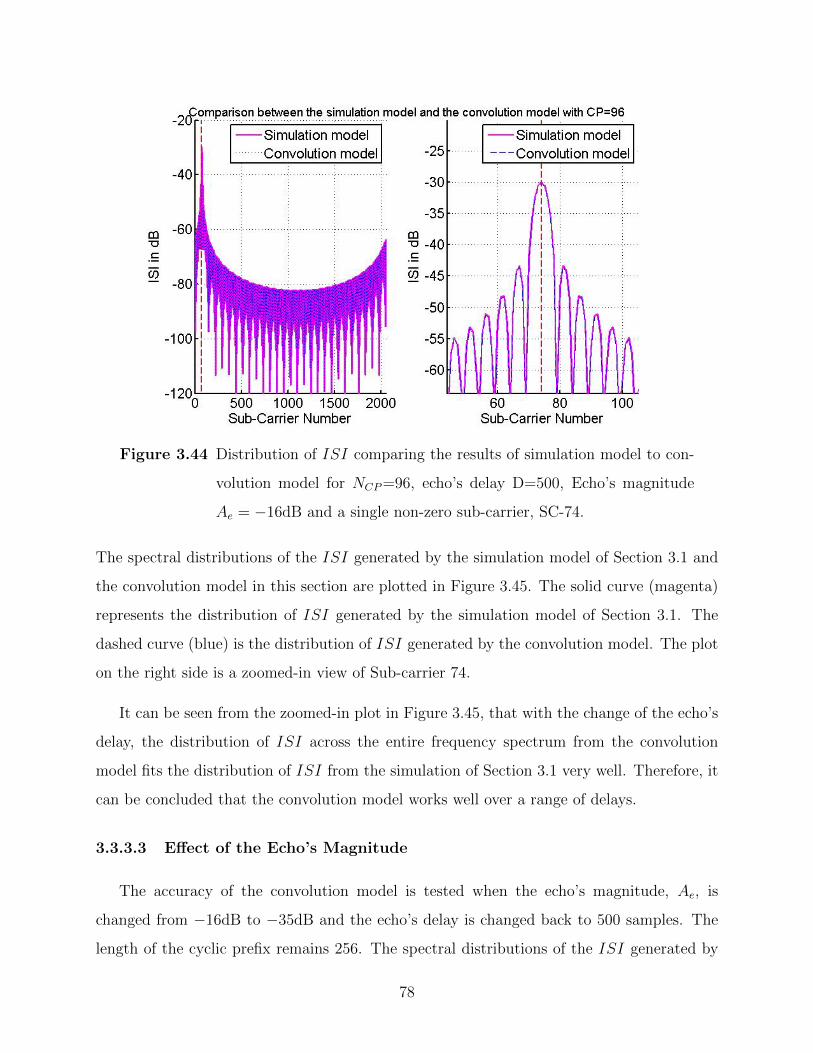
Figure 3.44 Distribution of ISI comparing the results of simulation model to con-
volution model for NCP=96, echo’s delay D=500, Echo’s magnitude
Ae = −16dB and a single non-zero sub-carrier, SC-74.
The spectral distributions of the ISI generated by the simulation model of Section 3.1 and
the convolution model in this section are plotted in Figure 3.45. The solid curve (magenta)
represents the distribution of ISI generated by the simulation model of Section 3.1. The
dashed curve (blue) is the distribution of ISI generated by the convolution model. The plot
on the right side is a zoomed-in view of Sub-carrier 74.
It can be seen from the zoomed-in plot in Figure 3.45, that with the change of the echo’s
delay, the distribution of ISI across the entire frequency spectrum from the convolution
model fits the distribution of ISI from the simulation of Section 3.1 very well. Therefore, it
can be concluded that the convolution model works well over a range of delays.
3.3.3.3 Effect of the Echo’s Magnitude
The accuracy of the convolution model is tested when the echo’s magnitude, Ae, is
changed from −16dB to −35dB and the echo’s delay is changed back to 500 samples. The
length of the cyclic prefix remains 256. The spectral distributions of the ISI generated by
78
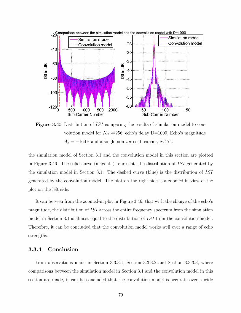
Figure 3.45 Distribution of ISI comparing the results of simulation model to con-
volution model for NCP=256, echo’s delay D=1000, Echo’s magnitude
Ae = −16dB and a single non-zero sub-carrier, SC-74.
the simulation model of Section 3.1 and the convolution model in this section are plotted
in Figure 3.46. The solid curve (magenta) represents the distribution of ISI generated by
the simulation model in Section 3.1. The dashed curve (blue) is the distribution of ISI
generated by the convolution model. The plot on the right side is a zoomed-in view of the
plot on the left side.
It can be seen from the zoomed-in plot in Figure 3.46, that with the change of the echo’s
magnitude, the distribution of ISI across the entire frequency spectrum from the simulation
model in Section 3.1 is almost equal to the distribution of ISI from the convolution model.
Therefore, it can be concluded that the convolution model works well over a range of echo
strengths.
3.3.4 Conclusion
From observations made in Section 3.3.3.1, Section 3.3.3.2 and Section 3.3.3.3, where
comparisons between the simulation model in Section 3.1 and the convolution model in this
section are made, it can be concluded that the convolution model is accurate over a wide
79

Figure 3.46 Distribution of ISI comparing the results of simulation model to con-
volution model for NCP=256, echo’s delay D=500, Echo’s magnitude
Ae = −35dB and a single non-zero sub-carrier, SC-74.
range of parameter values.
Therefore, if given the length of cyclic prefix, the echo’s delay, the echo’s strength and the
present sub-carrier number, the convolution model can be used to estimate the distributions
of ISI and IaSI. This convolution method will be modified and applied to the final “CP
length selection” model.
3.4 Aggregate Interference Corrupting a Single Sub-carrier
The ISI and IaSI for each single sub-carrier are estimated using the convolution method
introduced in Section 3.3.1. Of interest in this section is the aggregate interference corrupting
a sub-carrier when all active sub-carriers (i.e. Sub-carrier 74 to 1973) are present.
Let ISISC(ki) denote the component of ISI on Sub-carrier i that was generated by Sub-
carrier k. Similarly, let IaSISC(ki) denote the component of IaSI on Sub-carrier i that was
generated by Sub-carrier k. Aggregate interference corrupting Sub-carrier i is given by:
ISIAggregate(i) =1973∑k=74
ISISC(ki) +1973∑k=74
IaSISC(ki), i = 74, 75, ...1973. (3.40)
80

This equation is used in the next section to find the optimum length for the cyclic prefix
for a given echo delay.
81

4. Chapter4: Best Cyclic Prefix Length Selection
The objective of this chapter is to generate a computer program that can be used to
determine the best cyclic prefix length for an arbitrary cable network, given that the delays
and strengths of the echoes in the network are known.
An overview of the program will be given in the first section and then the program will be
explained step by step in the rest of this chapter. Finally, some test results will be presented.
4.1 Best CP Length Selection Program Overview
To introduce the program better, some background knowledge about the cable modem
upstream transmission system has to be mentioned first. Perhaps the most important thing
to know is the OFDMA signal is sent in frames from the CMs to CMTS. The CMTS assigns
the constellation order to each CM on a frame by frame basis. The constellation order is
assigned to maximize throughput for the SNR. If the SNR for a CM is low, then that CM is
assigned a low modulation order.
The program that calculates the best CP length must also calculate the optimum con-
stellation order for the CMs that share a frame. Then, after calculating the inter CM
interference, it computes the “useful data per minislot”1 for each of the possible CP lengths.
The CP length which offers the best “useful data per minislot” will be chosen to be the best
CP length for the frame.
1The “useful data per minislot” is a criteria set in the program judging the transmission quality and
efficiency, which depends on the number of transmitted bits per frame, CP length, FFT size and some other
parameters. Its definition and mathematical expression is included in Section 4.5.
82

Table 4.1 The input parameters for the best cyclic prefix length selection program
Parameters Notation Possible Values
CMTS
FFT size NFFT 2048, 4096
Sampling frequency FS 102.4MHz
Number of symbols
per frameNumsym No typical value
Number of sub-channels
per minislotQ 8, 16
User Group
The number of CMs
in the systemLcm
No larger than
the number of
active minislots
The average delay
of each CMdelayus
The number of
occupied minislots.Random
Which CM is assigned to
each minislotRandom
The best CP length selection program is designed to apply to a real cable modem com-
munication system. By analyzing the system’s parameters, the program can suggest a best
cyclic prefix length for this system. The input parameters and the brief flowchart of the
program will be introduced in the following sub-sections.
4.1.1 Input Parameters to the Program
The input parameters to the best CP length selection program are listed in Table 4.1.
At the CMTS side, the FFT size of the transmitted OFDMA signal (NFFT ), the sampling
frequency, the number of symbols per frame and the number of sub-channels per minislot are
known by the cable operator. The numbers of minislot occupied by users, the distribution
of the users’ delay and some other users’ information can be collected from the users’ trans-
mission history. These known variables are input to the best CP length selection program.
83

The cyclic prefix length is also an input to the system. DOCSIS3.1 allows the cyclic
prefix to have one of the following eleven lengths: 96, 128, 160, 192, 224, 256, 288, 320, 384,
512 and 640. The strategy used in the program is to try one cyclic prefix length at a time
and compute the transmission system’s useful data per minislot for that length. The length
that offers the highest useful data per minislot will be selected as the best CP length for the
system.
4.1.2 Flowchart of the Program
The flow chart of the working process of the best CP length selection program is shown
in Figure 4.1. For a single frame, the best CP length selection program starts by picking
the first possible CP length, i.e. 96, for computation. With this CP length, the program
will firstly estimate the aggregate interference for each sub-carrier, and then estimate the
aggregate interference for each minislot. Each minislot contains Q sub-carriers and the
largest interference of the Q sub-carriers is chosen to be the interference of the minislot.
With the interference of each minislot known, the next step is to compute the MER for
each minislot. Then, an optimum constellation order for each minislot is chosen based on
the calculated MER and the target BER. Finally, the useful data per minislot is calculated
using a mathematical method.
The algorithm is repeated for each possible CP length. After computing the useful
data per minislot for all of the allowable CP lengths, the CP length that offers the best
performance is selected as the optimum CP length for this frame.
The Best CP Length Selection Program will be introduced and explained step by step in
the following sections.
The program uses some results from Chapter 3. In the last section of Chapter 3, a
convolution model was developed to estimate the distributions of ISI and IaSI for each
sub-carrier. Equation (3.40) computes the aggregate interference corrupting a sub-carrier
when all active sub-carriers are present. These two results will be applied to the aggregate
interference computation in Section 4.2.
84

Figure 4.1 Flow chart of the working process of the Best CP Length Selection
Program
85

Table 4.2 The micro-reflections bound for dominant signal echo
Echo’s delay Echo Strength
≤0.5 µs -20 dBc
≤1.0 µs -25 dBc
≤1.5 µs -30 dBc
>2.0 µs -35 dBc
>3.0 µs -40 dBc
>4.5 µs -45 dBc
>5.0 µs -50 dBc
4.2 Aggregate Interference Computation
After choosing a candidate CP length, the next step for the Best CP Length Selection
Program is to compute the aggregate interference for each minislot.
A minislot cannot be shared among CMs. It can be empty or occupied by data from one
CM. Therefore, the Q sub-carriers in one minislot experience the same echo and therefore
the same delay. The delay of the echo for each CM is known to the CMTS.
According to DOCSIS3.1, the strength of the echo, Ae, depends on the echo’s delay. The
relationship between the echo’s delay and its maximum possible strength is tabulated in
Table 4.2. The strength of the echo encounted by a sub-carrier is taken to be the maximum
possible for the echo’s delay according to Table 4.2.
With the known echo delay and echo strength for each sub-carrier, the aggregate in-
terference of each sub-carrier can be computed using the convolution model developed in
Chapter 3. With the known cyclic prefix length NCP , echo’s strength Ae and echo’s delay
D for each sub-carrier, the convolution model is able to compute the aggregate interference
of every sub-carrier.
The next step is to find the aggregate interference for each minislot. The aggregate
interference for a minislot is taken to be the largest aggregate interference of the Q sub-
carriers in the minislot. That is because, if the system can guarantee the transmission
86

quality of the worst sub-carrier, the quality of all the Q sub-carriers in this minislot can be
guaranteed.
The MATLAB script which performs the aggregate interference computation function is
included in Appendix E.
4.3 MER Computation
Once the aggregate interference is known, the MER of each minislot can be computed.
MER is an acronym for modulation error ratio. Because of noise, the transmission and
constellation mapping are not always accurate. MER is a measure of the “fuzziness” of the
received symbol points in a constellation [33]. A larger MER value means better performance.
The mathematical expression for MER is
MER = 10× log10(Average Signal Power
Average Error Power) (4.1)
where the average signal power refers to the received signal power, which is the reference
power mentioned in Section 3.3.2. The average error power is the aggregate interference for
every minislot.
As discussed in Chapter 3, the reference power can be computed in three ways (referred
to as the largest case, the smallest case, and the average case).
For the largest case, the reference signal has power:
Reference−Powerlargest = (1 + Ae)2;
Since MER increases with signal power, the scenario with the largest reference power is the
best case in terms of performance. The MER value for minislot b in the best case is denoted
MERbest(b), which is given by:
MERbest(b) = 10× log10((1 + Ae)
2
Aggregate Interference(b)); (4.2)
For the worst case, the signal power is as small as possible which has the reference signal
power:
Reference−Powersmallest = (1− Ae)2;
87

The lowest signal power contributes to the worst case for the transmission system. The MER
value for minislot b in the worst case is denoted MERworst(b), which is given by:
MERworst(b) = 10× log10((1− Ae)
2
Aggregate Interference(b)); (4.3)
The average reference signal power is given by:
Reference−Powerave = 1 + A2e.
In this case, the MER value for minislot b is denoted MERave(b), which is given by:
MERave(b) = 10× log10(1 + A2
e
Aggregate Interference(b)); (4.4)
All three cases are considered separately. To make the explanation clearer, only the average
case is included in the model description. However, all three cases are included in the results.
4.4 Constellation Type Selection
The next step is to choose a suitable constellation type for each minislot.
The CMTS is able to assign any constellation order listed in Table 4.3 to any CM. To
ensure the signal transmission quality, the constellation order must meet the requirement
of Bit Error Rate (BER) and therefore MER. The possible upstream constellation types in
DOCSIS 3.1 are listed in Table 4.3. The table lists the constellation orders, M , which are
perhaps obvious and also the number of data bits per symbol, k.
For those minislots that don’t have interference, the highest constellation order will be
chosen to guarantee the fastest transmission speed. For the minislots that suffer from inter-
ference, MERs have been computed in the last section.
BER must be taken into consideration in choosing a constellation type for the minislot
with interference. BER is an acronym for Bit Error Rate, which is the ratio of bits received
in error to the total number of bits received or processed over a defined amount of time [34].
To derive the relationship between BER, MER and constellation order, another variable,
SER which is an acronym for Symbol Error Rate is introduced [35]. SER is the ratio of
88

Table 4.3 All possible constellation orders for the upstream transmission
Constellation Type M k
QPSK 4 2
8-QAM 8 3
16-QAM 16 4
32-QAM 32 5
64-QAM 64 6
128-QAM 128 7
256-QAM 256 8
512-QAM 512 9
1024-QAM 1024 10
2048-QAM 2048 11
4096-QAM 4096 12
symbols received in error to the total number of symbols received over a given amount of
time.
The book “Digital Communications” [36] provides the relationship between BER and
SER as:
BER =1
k(1− 1√
M)× SER; (4.5)
where k is the number of bits per symbol and M = 2k is the modulation order, which is
synonymous to the constellation type.
There is no specific mathematical equation to describe the relationship between SER and
MER, but the upper bound of SER can be expressed mathematically as:
SER ≤ 4Q(
√3kEb
(M − 1)N0
); (4.6)
where EbN0
is the average SNR per bit (i.e. ratio of the average energy per bit to the power in
the noise over a 1 Hz bandwidth). In this case Q represents the “Q-function”, which is the
tail probability of the standard normal distribution [37]. Formally, the Q-function is defined
89
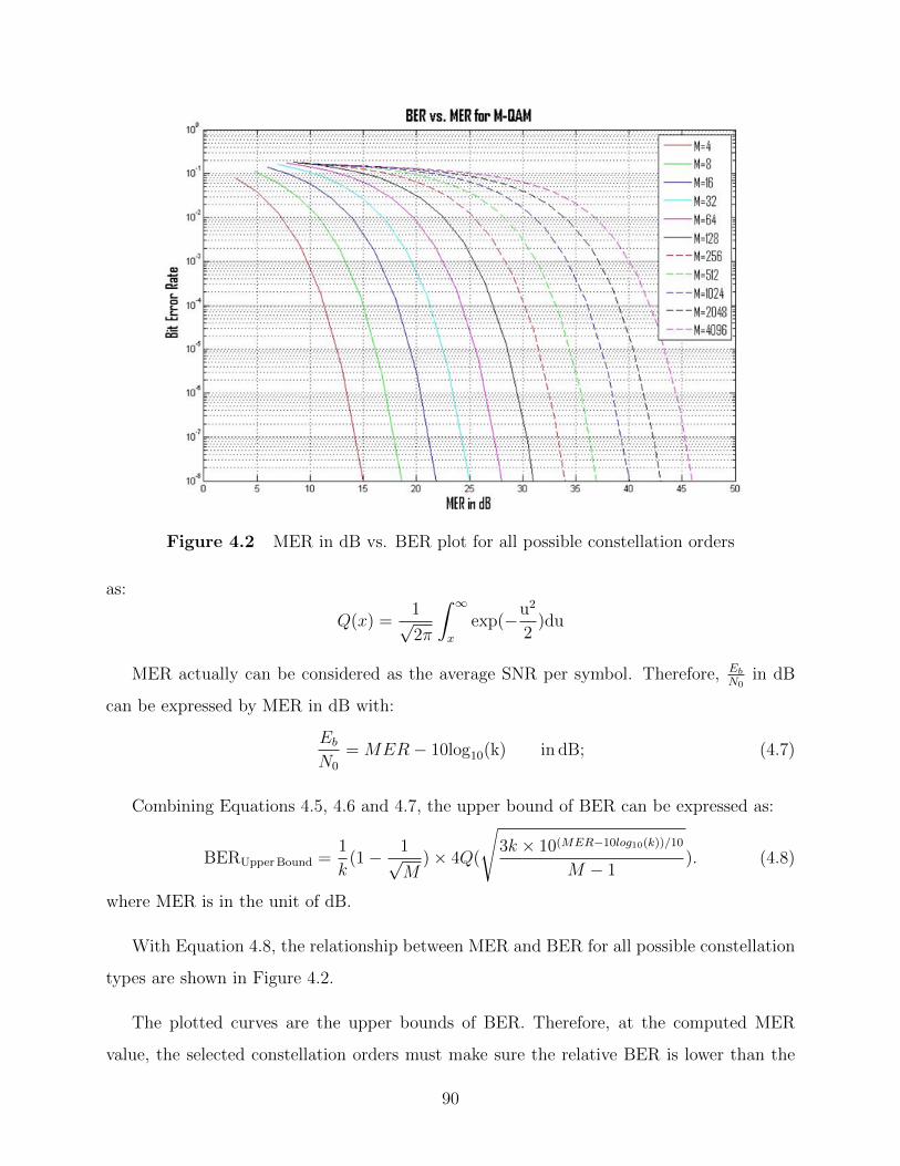
Figure 4.2 MER in dB vs. BER plot for all possible constellation orders
as:
Q(x) =1√2π
∫ ∞x
exp(−u2
2)du
MER actually can be considered as the average SNR per symbol. Therefore, EbN0
in dB
can be expressed by MER in dB with:
EbN0
= MER− 10log10(k) in dB; (4.7)
Combining Equations 4.5, 4.6 and 4.7, the upper bound of BER can be expressed as:
BERUpperBound =1
k(1− 1√
M)× 4Q(
√3k × 10(MER−10log10(k))/10
M − 1). (4.8)
where MER is in the unit of dB.
With Equation 4.8, the relationship between MER and BER for all possible constellation
types are shown in Figure 4.2.
The plotted curves are the upper bounds of BER. Therefore, at the computed MER
value, the selected constellation orders must make sure the relative BER is lower than the
90

Figure 4.3 An example to show how to choose a suitable constellation type
bound. To guarantee the transmission speed, the highest satisfactory constellation order is
chosen. For example, consider a scenario in which the required BER value is no larger than
10−7, which is the horizontal dashed line in Figure 4.3 and the computed MER value is 45
dB, shown as the vertical dashed line. In this scenario, to ensure the BER requirement is
met, all the constellation types in the shadowed part can be chosen for this minislot (all
except 4096-QAM). Among the available constellation orders, the largest one, 2048-QAM is
able to offer the highest data rate. Therefore, 2048-QAM is selected for each minislot.
The Matlab scripts that compute the constellation order selection is included in Ap-
pendix F.
4.4.1 The Usability of BER and MER Plot
The BER vs. MER curves plotted in Figure 4.3 were generated under the assumption
that the noise is additive, white and Gaussian distributed (i.e. AWGN) [38]. However,
the distribution of the aggregate interference has to be considered and may or may not
be Gaussian. Therefore, for the BER vs. MER curves plotted in Figure 4.3 to apply, the
91

Figure 4.4 The histograms of errors in active sub channel for QPSK with
NCP=256, D=500, Ae=-16dB
distribution of the interference must be shown to be Gaussian or at least nearly Gaussian.
With the help of the interference distribution model introduced in Section 3.1.3 on page
42, the differences between the transmitted and received signals in the active sub carriers
can be computed. The histograms of the real parts and the imaginary parts of errors are
shown in Figure 4.4 with a sample size of 1,900,000. These histogram plots show the shape
of the distribution of the error.
To check whether the distribution of the interference follow the Gaussian distribution or
not, the ideal Gaussian distribution is plotted together with the histograms. The probability
density function of Gaussian noise is given by:
PDF =1
σ√
2πe−
(x−µ)2
2σ2 (4.9)
where µ is the mean and σ is the standard deviation. In Figure 4.4, the bold curves in red,
which follow the shapes of the histograms, are the ideal Gaussian distribution shapes. From
Figure 4.4, it can be seen that both real and imaginary histograms have a nearly Gaussian
shape, which means the error due to interference is nearly Gaussian distributed.
92

From experimental observation, it has been shown that the constellation type, echo’s
delay, echo’s magnitude and cyclic prefix length do not affect the shape of the Gaussian
distribution. Therefore, the BER vs. MER curves plotted in Figure 4.2 can be used for
choosing the best constellation type.
4.5 Best CP Length Selection
With the best constellation type for every minislot chosen, the final step is to select a
best cyclic prefix length for the system. The cyclic prefix length must be the same for all
the minislots in a frame.
The selection criteria is to compute the useful data per minislot for the whole frame. The
equation is given by:
R =N∑i=1
k ×NS ×Q×NFFT
NFFT +NCP
× 1
N; (4.10)
where N is the number of minislots per frame, k is the number of transmitted bits per
symbol, NS is the number of symbols per frame, and in this case Q is the number of sub-
carriers per minislot. Therefore, k × NS represents the number of bits per sub-carrier per
frame.
Since there are Q sub-carriers per minislot, k×NS×Q represents the number of bits per
minislot.
Since N is the number of minislots per frame, summing over all minislots, i.e.∑N
i=1 k ×
NS ×Q, yields the number of bits per frame.
NFFT is the number of points used in the FFT, which is also the number of samples in a
symbol, and NCP refers to the cyclic prefix length (i.e. the number of samples in the cyclic
prefix). Therefore, NFFTNFFT+NCP
is the ratio of useful symbol length to total symbol length.
Multiplying this ratio by the number of bits per frame,∑N
i=1 k×NS×Q× NFFTNFFT+NCP
provides
the ratio of useful number of bits per frame, which is referred to as “useful data”.
Dividing the transmitted useful data by the number of minislots N gives the useful data
per minislot, which is the selection criteria for the best CP length and is denoted as R.
93

Table 4.4 Parameters used for testing
Parameters Value
NFFT 2048
CP 96,128,160,192,224,256,288,320,384,512,640
FS 102.4MHz
Numsym 16
BER ≤ 10−8
4.6 Program Testing
4.6.1 Parameters Used for Testing
For the purposes of testing, the users are divided into four groups. Each with 237 users.
Each user is assigned only one minislot. The four user groups are distinguished by the
distribution of their echo’s delay. The description of the user groups and the relevant results
are included in the following four sections.
The parameters used in the simulation are listed in Table 4.4. The NFFT used for testing
is 2048, which means the value for Q, which is the number of sub-carriers per minislot, must
be 8. Had 4096 been used for NFFT , then Q would have to be 16. FS is the sampling rate,
which is 102.4MHz. Numsym is the number of symbols per frame, which must be between 6
and 36. It is chosen to be 16. The BER must be less than 10−8.
In Section 4.3, three different cases of MER are discussed. The best case MER is com-
puted with the largest interference power. The worst case MER has the smallest reference
power and the average MER with average reference power. Although only the average case
is analyzed in the previous sections, all the three cases are actually been considered and
computed in the program. The computation for the three cases use the same algorithm but
different MERs. Therefore, the program will output the computed results and plots of the
three cases, which will indicate in the testings.
94

Figure 4.5 Distribution of echo’s delay in user group 1
4.6.2 Uniformly Distributed Echo’s Delays
The 237 users in the first user group has uniformly distributed echo delays. A histogram
of delays for the echo is plotted in Figure 4.5. The histogram shows the echo’s delays are
uniformly distributed from 0µs to 6.25µs.
After the processing of the best CP length selection system, the useful data per minislot
for every possible CP length is computed and given in Figure 4.6. As discussed in Section 4.3,
the best CP length selection system computed three cases: the best case, the average case
and the worst case. Figure 4.6 has three curves: where the solid blue line tagged with circles
represents the best case, the dash-dot red line tagged with stars represents the average case
and the untagged dashed green line represents the worst case. As Figure 4.6 shows, the three
curves are almost the same for all CPs.
For all the three cases, the curves increase slightly from CP=96 to CP=128 and then
keep dropping. That is because the overhead increases with increasing CP length.
95

Figure 4.6 The useful data per minislot for user group 1
For the three cases, when CP = 128, the useful data per minislot has the largest value.
Therefore, the best CP length for this group is 128.
Since some users experience more interference than others, they need to be assigned
different modulation orders in order to maximize the useful data per frame. For CP=128,
Table 4.5 shows the utilization of constellation type. It indicates that highest order modu-
lation that 7 users can support is 1024-QAM. 31 can support at most 2048-QAM and 199
users can support 4096-QAM.
4.6.3 Gaussian Distributed Echo’s Delays
The second group of users is characterized by the echo’s delays for the users having a
truncated Gaussian distribution. Figure 4.7 shows the distribution of echo’s delays among
the users in the group. The delay for each user was drawn from a Gaussian distribution with
a mean of 3.125µs and a standard deviation of 1, truncated at 0 and 6.25µs.
After the processing of the best CP length selection system, the useful data per minislot
96

Table 4.5 Number of users for each constellation type for user group 1
Constellation Type Number of users
QPSK 0
8-QAM 0
16-QAM 0
32-QAM 0
64-QAM 0
128-QAM 0
256-QAM 0
512-QAM 0
1024-QAM 7
2048-QAM 31
4096-QAM 199
Figure 4.7 Distribution of echo’s delay in user group 2
97

Figure 4.8 The useful data per minislot for user group 2
for every possible CP length was computed and plotted in Figure 4.8. Figure 4.8 also has
three curves: where the solid blue line tagged with circles represents the best case, the dash-
dot red line tagged with stars represents the average case and the untagged dashed green
line represents the worst case. The three curves are almost the same for all except two values
of CP: CP=96 and 128. However, even in the two exceptions, there is very little difference.
For all the three cases, the curves increase slightly from CP=96 to CP=128 and then
drop slightly from CP=128 to CP=224. For CP > 224, the curves drop quickly at a constant
rate. For the three cases, the useful data per minislot has the largest value for CP=128.
Therefore, choose CP=128 for this group.
Table 4.6 shows the utilization of modulation orders for CP=128. Note that in this
scenario fewer users can support 4096-QAM.
98

Table 4.6 Number of users for each constellation type for user group 2
Constellation Type Number of users
QPSK 0
8-QAM 0
16-QAM 0
32-QAM 0
64-QAM 0
128-QAM 0
256-QAM 0
512-QAM 0
1024-QAM 17
2048-QAM 59
4096-QAM 161
4.6.4 Compact Distribution of Echo’s Delays with “Outliers”
The third user group has echo’s delays concentrated in a relatively short time range with
a few “outliers”. As Figure 4.9. shows, the distribution of most of the users echo’s delays
uniformly distributed between 0µs and 3µs and 20 “outliers” users with an echo’s delay
6.25µs.
After the processing of the best CP length selection system, the useful data per minislot
for every possible CP length was computed and plotted in Figure 4.10. Figure 4.10 also
has three curves: where the solid blue line tagged with circles represents the best case, the
dash-dot red line tagged with stars represents the average case and the untagged dashed
green line represents the worst case. As Figure 4.10 shows, the three curves are very nearly
the same except at CPs with values CP=96 and 128, where they are still quite similar.
For all the three cases, the curves increase sharply from CP=96 to CP=128 and then
drop slightly from CP=128 to CP=224. For CP > 224, the curves drop relatively quickly.
For the three cases, when CP = 128, the useful data per minislot has the largest value.
Therefore, choose CP=128 for this group.
99

Figure 4.9 Distribution of echo’s delay in user group 3
Figure 4.10 The useful data per minislot for user group 3
100

Table 4.7 Number of users for each constellation type for user group 3
Constellation Type Number of users
QPSK 0
8-QAM 0
16-QAM 0
32-QAM 0
64-QAM 0
128-QAM 0
256-QAM 0
512-QAM 0
1024-QAM 13
2048-QAM 59
4096-QAM 165
Table 4.7 shows the utilization of modulation order. Comparison with Table 4.6 shows
that groups 2 and 3 have very similar utilization of modulation order.
4.6.5 Compact Distribution of Echo’s Delays with Large Mean
The last user group has the echo’s delays uniformly distributed between 3.25µs to 6.25µs
with one outlier having delay of 0.25µs (Shown in Figure 4.11).
After the processing of the best CP length selection system, the useful data per minislot
for every possible CP length is computed and plotted in Figure 4.12. Figure 4.12 also has
three curves: where the solid blue line tagged with circles represents the best case, the dash-
dot red line tagged with stars represents the average case and the untagged dashed green
line represents the worst case. As Figure 4.12 shows, the three curves are almost the same.
For all the three cases, the curves drop as CP increases. When CP = 96, the useful data
per minislot has the largest value. Therefore, choose CP=96 for this group. In this case, the
longest delay is 6.25us which is 640 in samples. If the CP length is chosen to be 640, which
can cover the longest delay length, the computed useful data per minislot is about 1170 bits.
101

Figure 4.11 Distribution of echo’s delay in user group 4
Figure 4.12 The useful data per minislot for user group 4
102

Table 4.8 Number of users for each constellation type for user group 4
Constellation Type Number of users
QPSK 0
8-QAM 0
16-QAM 0
32-QAM 0
64-QAM 0
128-QAM 0
256-QAM 0
512-QAM 0
1024-QAM 0
2048-QAM 0
4096-QAM 237
Compare to the best CP chosen by the program, the performance is not so good.
Table 4.8 shows the utilization of modulation order for this group. All users can be
4096-QAM. The reason for this is the echo strength are weaker for the larger delays shown
in Figure 4.11. One would think the CP should be longer for longer delays, but the strength
of the echos are so weak, they do not need to be protected by the cyclic prefix.
103

5. Chapter5: Discussion and Conclusion
5.1 Results Discussion and Further Test
Four hypothetical cable systems were tested with the Best CP Selection Program in
Section 4.6. The program suggested a best CP for each system based on the computed useful
data per minislot. According to the analysis of each user group, the results are reasonable.
However, the program is not perfect. The only two sources of noise considered in the
system are the Intra Symbol Interference and the Inter Symbol Interference. The channel
noise, the coding error and many other performance degrading effect factors are not included.
Comparing with the noise existing in a real system, the noise considered in this program is
much less. Dealing with less noise, a shorter CP length is enough to protect the transmission
quality. The analysis of the four users groups in Section 4.6 show, the optimum CP lengths
are no larger than 128. More tests should be conducted to verify the program works properly
for the user groups with more noise.
Instead of adding more noise to the transmission system, the program could be tested by
increasing the program’s accuracy. To achieve this, the BER requirement should be moved
from 10−8 to 10−20.
A test was performed leaving the other parameters of the program unchanged and testing
the first user group again with the BER requirement of 10−20. Result of this test is shown
in Figure 5.1.
As discussed in Section 4.3, the best CP length selection program considered three cases:
the best case, the average case and the worst case. Figure 5.1 also has three curves: where
104

Figure 5.1 The useful data ratio per minislot for each CP length with BER re-
quirement to be 10−20
the solid blue line tagged with circles represents the best case, the dash-dot red line tagged
with stars represents the average case and the untagged dashed green line represents the
worst case. As Figure 5.1 shows, the three curves are almost the same for all CPs.
For all the three cases, the curves increase slightly from CP=96 to CP=224 and then
drop slightly from CP=224 to CP=320. Finally, the curves keep dropping quickly. For the
three cases, when CP = 224, the useful data per minislot has the largest value. Therefore,
choose CP=224 for this group.
Table 5.1 shows the utilization of constellation type. It indicates that 10 users can support
1024-QAM. 47 can support 2048-QAM and 180 users can support 4096-QAM.
Comparison of this with the test done for BER < 10−8 shows there is no significant dif-
ference, but the number of users who can support the highest modulation order is decreased.
That is because with a more strict BER requirement, less interference can be tolerated and a
longer CP length is needed as well as lower constellation orders are necessary for protection
105

Table 5.1 Number of minislots for each constellation type with echo delays uni-
formly distributed for BER no larger than 10−20
Constellation Type Number of minislots
QPSK 0
8-QAM 0
16-QAM 0
32-QAM 0
64-QAM 0
128-QAM 0
256-QAM 0
512-QAM 0
1024-QAM 10
2048-QAM 47
4096-QAM 180
against interference.
Therefore, with stricter requirements or with more noise, the best CP length may change.
This thesis provides a framework for calculating the best CP length for any cable system.
From the testing performed in this study, the system appears to be to be reliable.
5.2 Future Work
In this thesis, a program to find the best CP length for an upstream transmission system
was developed. The program can help to maximize throughput in DOCSIS 3.1 systems by
balancing the transmission efficiency and quality.
However, the program developed in this thesis is meant to be a ‘proof of concept’. Some
factors have been ignored to simplify the analysis and to make the main idea more clear and
logical. For example, the bit error rate considered in this thesis does not consider the effect
of LDPC encoding. Therefore, for future study, all the missed details can be added to make
the model more precise.
106

• The roll-off period (RP) is a repetition of part of the OFDMA symbol and is attached
to the end of each symbol. It should be included in the signal construction. Together
with CP, RP will affect the cyclic prefix length selection by modifying the ISI and IaSI.
• Some components of noise were ignored by the system developed in this thesis. Com-
ponents, such as the channel noise could be added in future studies.
• Not all the processes that affect the system performance were considered in this study.
The missing processes should be added to the system. According to the rules of DOC-
SIS3.1, there is an error correction process that uses Low-Density Parity-Check, LDPC
for short. LDPC is applied to the received signal to correct bit errors. Therefore, MER
should be computed after error correction. Inclusion of LDPC may affect the choice
for CP length.
The system can be improved not only by adding more details, but also by being mul-
tifunctional. For example, it could be modified to place more weight on VIP customers’
transmission quality and speed. If some users want to pay more to guarantee his/her cable
modem transmission quality and speed, when the system starts to choose a suitable CP
length for this user group, the system should make sure the paid customers can experience
4096-QAM constellation type and a high quality transmission.
Although a lot of work needs to be done to make the system perfect, the current work
provides a good base which can be expanded in future studies.
107

A. DOCSIS 3.1 Table 5-2
Figure A.1 Table 5 2 - Typical Upstream RF Channel Transmission Characteristics
108

B. The Main MATLAB Script for the ISI
Distribution Simulation Model
% this is the main MatLab program to discover
%the ISI distribution
clear all;
close all;
%% System parameters
N_FFT = 2048; % FFT size in DOCSIS3 .1 upstream is
%2048 or 4096
N_CP = 256; % cyclic prefix length
%either 96,128,160,192,224,256,288,320,384,512,640
N_RP = 0; % number of roll-off samples, either
% 0,32,64,96,128,160,192,224
Mod_type = ’QPSK’;
Sub_chan = 74:74; % sub-channel mapping
Ae= -16; % the echo strength, in dB
D=500; % echo delay time
time=100; % run 100 times and compute the average
W=length(Sub_chan);
for n=1:time
%% transmitter
% OFDM signal 1 and 2
[tx_1]=OFDM_Tx(N_FFT,N_CP,N_RP,Sub_chan,Mod_type);
109

[tx_2]=OFDM_Tx(N_FFT,N_CP,N_RP,Sub_chan,Mod_type);
tx=[tx_1;tx_2];% composite signal
%% channel
[rx,h_equ]=Channel(tx,D,Ae);
%% compute the ISI
Main_path_sym2=tx(2*N_CP+N_FFT+1:2*(N_CP+N_FFT));
%The main path of Symbol 2
error=rx(2*N_CP+N_FFT+1:D+N_CP+N_FFT)...
-Main_path_sym2(1:D-N_CP);
%The ISI segment in Symbol 2
e=[error;zeros(N_FFT-length(error),1)];
%To the purpose of FFT, extend ISI segment with 0s
E(n,1:N_FFT)=1/sqrt(N_FFT)*...
abs(fft(e.*exp(1j*pi*[0:N_FFT-1]).’));
ISI(n,1:N_FFT) = E(n,1:N_FFT).^2;
%% Reference power
[rx_noISI,h_equ]=Channel(tx,200,Ae);
rx_sig=rx_noISI(2*N_CP+N_FFT+1:2*(N_CP+N_FFT));
%The received Symbol 2 without ISI
reference_power = sum(abs(rx_sig).^2);
%% ISI in dB
ISIdB= ISI/reference_power;
end
Time_ISI=sum(ISIdB)/time;
110

figure(1);
plot(1:N_FFT,10*log10(Time_ISI));
hold on;
S=[’ISI distribution with N_C_P=...
’,num2str(N_CP),’, Delay D=’,num2str(D),...
’, Echo strength A_e=-16dB, Sub-carrier’,...
num2str(Sub_chan(1))];
title(S,’fontsize’, 14 );
xlabel(’Sub-Carrier Number’,’fontsize’, 16 );
ylabel(’ISI in dB’,’fontsize’, 16 );
plot([74 74], get(gca, ’YLim’),’--r’,...
’linewidth’,2);
axis([0 N_FFT -120 -20]);
set(gca, ’fontsize’, 16 );
set(gca,’linewidth’,2)
grid on;
111

C. The Main MATLAB Script for the ISITOTAL
Distribution Corroboration Model
% this is the main MatLab program to collaborate
% the distribution of ISI_TOTAL
clear all;
close all;
%% System parameters
N_FFT = 2048; % FFT size in DOCSIS3 .1 upstream is
% 2048 or 4096
N_CP = 256; % cyclic prefix length
%either 96,128,160,192,224,256,288,320,384,512,640
N_RP = 0; % number of roll-off samples, either
% 0,32,64,96,128,160,192,224
Mod_type = ’QPSK’;
Sub_chan = 74:74; % sub-channel mapping
Ae= -16; % echo strength, in dB
D=500; % echo delay time
time = 100; % run 100 times and compute the average
W = length(Sub_chan); % used channel width
for n=1:time
%% transmitter
% OFDM symbol 1 and 2
[tx_1]=OFDM_Tx(N_FFT,N_CP,N_RP,Sub_chan,Mod_type);
112

[tx_2]=OFDM_Tx(N_FFT,N_CP,N_RP,Sub_chan,Mod_type);
tx=[tx_1; tx_2];% composite signal
%% channel
[rx,h_equ]=Channel(tx,D,Ae);
%% receiver
[rx_info]=OFDM_Rx(rx,N_FFT,N_CP,Sub_chan,Mod_type,h_equ);
%The constellation constructed from the received Symbol 2
%% reference power
[rx_ref,h_ref]=Channel(tx,200,Ae);
[rx_info_ref]=OFDM_Rx(rx_ref,N_FFT,N_CP,...
Sub_chan,Mod_type,h_ref);
% The constellation constructed from the
% received no-ISI Symbol 2
reference_power = sum(abs(rx_info_ref).^2);
%% ISI_TOTAL indB
ISI_TOTALdB(n,1:N_FFT)=abs(rx_info - rx_info_ref).^2...
/reference_power;
end
freq_ISI=sum(ISI_TOTALdB)/time;
figure(1);
plot(1:N_FFT,10*log10(freq_ISI));
hold on;
S=[’ISI_T_O_T_A_L distribution with N_C_P=’...
,num2str(N_CP),’, Delay D=’,...
num2str(D), ’, Echo strength A_e=-16dB,...
113

Sub-carrier’,num2str(Sub_chan(1))];
title(S,’fontsize’, 14 );
xlabel(’Sub-Carrier Number’,’fontsize’, 16 );
ylabel(’ISI in dB’,’fontsize’, 16 );
plot([74 74], get(gca, ’YLim’),’--r’,’linewidth’,2);
axis([0 N_FFT -120 -20]);
set(gca, ’fontsize’, 16 );
set(gca,’linewidth’,2)
grid on;
114

D. The MATLAB Script for the ISI Distribution
Convolution Model
% this is the MatLab program of the convolution model
%to discover the ISI distribution
clear all;
close all;
%% System parameters
N_FFT=2048;
N_CP=256; %cyclic prefix length
D=500; %the echo’s delay
Ae=-16;%the echo’s magnitude in dB
Sub_chan=74; %the only non-zero sub-carrier
time=100;
%% Build the extracting mask in frequency domain
L=D-N_CP; %length of ones
mask=[zeros(1,N_FFT-L),ones(1,L)];%mask in time domain
MASK=1/sqrt(N_FFT)*...
abs(fft(mask.*exp(1j*pi*[0:N_FFT-1])));
%mask in frequency domain
Mshift=circshift(MASK,[0 -N_FFT/2]);
%shift for circular convolution
%% Build the ISI segment in frequency domain
115

echo(1:N_FFT)=zeros(1,N_FFT);
echo(Sub_chan)=10^(Ae/20)*exp(1j*rand(1)*2*pi);
% The transmitted signal has magnitude of
% Ae dB and a random phase
%% Do circular convolution
ISI_seg(1:N_FFT)=1/sqrt(N_FFT)*...
cconv(Mshift,echo(1:N_FFT),N_FFT);
% Compute the ISI power
ISI(1:N_FFT)=ISI_seg(1:N_FFT).^2;
%% Compute the reference power
% study the received power in
% the best, average and worst cases
Pref_best=(1+10^(Ae/20))^2;
Pref_ave=1+(10^(Ae/20))^2;
Pref_worst=(1-10^(Ae/20))^2;
%% Compute ISI in dB
ISIdB_best(1:N_FFT) = ISI(1:N_FFT)/Pref_best;
ISIdB_ave(1:N_FFT) = ISI(1:N_FFT)/Pref_ave;
ISIdB_worst(1:N_FFT) = ISI(1:N_FFT)/Pref_worst;
Est_ISI_best = abs(ISIdB_best);
Est_ISI = abs(ISIdB_ave);
Est_ISI_worst = abs(ISIdB_worst);
%% Plot
figure(1);
plot(10*log10(Est_ISI_best));
hold on;
S=[’The ISI Distribution with N_C_P=’,...
num2str(N_CP),’, Delay D=’,num2str(D),...
116

’, Echo strength A_e=’ num2str(Ae),...
’, Sub-carrier’,num2str(Sub_chan),...
’ for the Average Case’];
title(S,’fontsize’, 14 );
xlabel(’Sub-Carrier Number’,’fontsize’, 16);
ylabel(’ISI in dB’,’fontsize’, 16 );
plot([74 74], get(gca, ’YLim’),’--r’,...
’linewidth’,2);
axis([0 N_FFT -120 -20]);
set(gca, ’fontsize’, 16 );
set(gca,’linewidth’,2)
grid on;
figure(2);
plot(10*log10(Est_ISI));
hold on;
S=[’The ISI Distribution with N_C_P=’,...
num2str(N_CP),’, Delay D=’,num2str(D),’...
, Echo strength A_e=’ num2str(Ae),...
’, Sub-carrier’,num2str(Sub_chan),...
’ for the Best Case’];
title(S,’fontsize’, 14 );
xlabel(’Sub-Carrier Number’,’fontsize’, 16);
ylabel(’ISI in dB’,’fontsize’, 16 );
plot([74 74], get(gca, ’YLim’),’--r’,...
’linewidth’,2);
axis([0 N_FFT -120 -20]);
set(gca, ’fontsize’, 16 );
set(gca,’linewidth’,2)
grid on;
117

figure(3);
plot(10*log10(Est_ISI_worst));
hold on;
S=[’The ISI Distribution with N_C_P=’,...
num2str(N_CP),’, Delay D=’,num2str(D),...
’, Echo strength A_e=’ num2str(Ae),...
’, Sub-carrier’,num2str(Sub_chan),...
’ for the Worst Case’];
title(S,’fontsize’, 14 );
xlabel(’Sub-Carrier Number’,’fontsize’, 16 );
ylabel(’ISI in dB’,’fontsize’, 16 );
plot([74 74], get(gca, ’YLim’),’--r’,...
’linewidth’,2);
axis([0 N_FFT -120 -20]);
set(gca, ’fontsize’, 16 );
set(gca,’linewidth’,2)
grid on;
118

E. The MATLAB Script for the Aggregate
Interference Computation Function of the
Final Model
function [ISI_corrupt,Ae] = frame_effect(CP, N_FFT,...
delay_us, delay_sample, L_cm, Bound_up, Bound_low)
Q=Bound_low(1)-Bound_up(1)+1;
for a = 1:length(CP)
N_CP = CP(a); %cyclic prefix length
for b = 1:L_cm
D = delay_sample(b);
%echo delay for each cable modem
if N_CP < D
% set the echo magnitude in dB
if delay_us(b) <= 0.5
Ae(b,a) = -16;
elseif delay_us(b) <= 1
Ae(b,a) = -22;
elseif delay_us(b) <= 1.5
Ae(b,a) = -29;
elseif delay_us(b) > 4.5
Ae(b,a) = -51;
elseif delay_us(b) > 3
119

Ae(b,a) = -42;
else
Ae(b,a) = -35;
end
%Build the extracting mask in frequency domain
L=D-N_CP;
mask=[zeros(1,N_FFT-L),ones(1,L)];
MASK=1/sqrt(N_FFT)*...
abs(fft(mask.*exp(1j*pi*[0:N_FFT-1])));
Mshift=circshift(MASK,[0 -N_FFT/2]);
for c=Bound_up(b):Bound_low(b)
%Build the ISI segment in frequency domain
echo(1,1:N_FFT)=zeros(1,N_FFT);
echo(1,c)=10^(Ae(b,a)/20)*...
exp(1j*rand(1)*2*pi);
%The transmitted signal has magnitude of
%Ae dB and a random phase
%Do circular convolution
ISI_seg(1,1:N_FFT)=1/sqrt(N_FFT)*...
cconv(Mshift,echo(1,1:N_FFT),N_FFT);
%The distribution of ISI_TOTAL
% for each sub-carrier
ISI(c,1:N_FFT)=abs(2*(ISI_seg).^2);
figure(2);
plot(10*log10(ISI(c,1:N_FFT)));
axis([0 N_FFT -130 -30]);
title(’The plot of ISI spread ...
120

over all sub channels’);
xlabel(’Subchannel Number’);
ylabel(’ISI value’);
grid on;
end
else
ISI(Bound_up(b):Bound_low(b),1:N_FFT)=...
zeros(Q,N_FFT);
end
end
%Compute the ISI corrupted in each sub-carrier
ISI_corrupt(a,1:N_FFT)=sum(ISI);
end
121

F. The MATLAB Script for the Constellation
Order Function of the Final Model
function [k_element] = sel_k...
(ISI_corrupt, Bound_up, Bound_low, a, b, Ae)
%find the worst case MER for each cable modem
%find the largest ISI for each cable modem first
CM_ISI = max(ISI_corrupt(a,Bound_up(b):Bound_low(b)));
%Compute the reference power
%study the received power in the best,average
%and worst cases
Pref_best=(1+10^(Ae(b,a)/20))^2;
Pref_ave=1+(10^(Ae(b,a)/20))^2;
Pref_worst=(1-10^(Ae(b,a)/20))^2;
% Compute three cases MER for each CM
MER_best = 10*log10(Pref_best/CM_ISI);
MER_ave = 10*log10(Pref_ave/CM_ISI);
MER_worst = 10*log10(Pref_worst/CM_ISI);
MER=[MER_best MER_ave MER_worst];
for i=1:length(MER)
%select the best constellation order
122

k = 2:12;
M = 2.^k; %constellation type
Eb_N0 = MER(i)-10.*log10(k);
SER = 4*qfunc(sqrt((3*k.*10.^(Eb_N0/10))./(M-1)));
BER = 1./k.*(1-1./sqrt((M))).*SER;
% compute the BER with the given MER
f2 = find(BER<=10^-8);
% find the index of BERs no larger than 10^(-8)
if isempty(f2) == 1
k_element(i) = 0;
else
k_element(i) = f2(length(f2))+1;
%k is 1 larger than the index in the array
end
end
123

References
[1] California-Cable and Telecommunications-Association, “History of cable,” 2015. Com-
pany Website Homepage (http://www.calcable.org/learn/history-of-cable/).
[2] L. Harte, Introduction to Cable Television (CATV): Analog and Digital Television and
Modems. Althos, 2nd ed., 2007.
[3] CableLabs, Data-Over-Cable Service Interface Specifications DOCSIS 3.1. Cable Tele-
vision Laboratories, Inc., 2014.
[4] M. Kalman and B. Girod, “Modeling the delays of successively-transmitted internet
packets,” in Multimedia and Expo, 2004. ICME’04. 2004 IEEE International Conference
on, vol. 3, pp. 2015–2018, IEEE, 2004.
[5] M. Sadiku and C. Aduba, “Cable modem technology,” Potentials, IEEE, vol. 19, pp. 26–
27, August 2002.
[6] C. Franklin, “How cable modems work,” Apr. 2016.
[7] B. Berscheid, “FPGA-Based DOCSIS Upstream Demodulation,” July 2011.
[8] S. P. Crosby and G. K. Noreen, “Internet-based interactive radio system for use with
broadcast radio stations,” Sept. 30 2003. US Patent 6,628,928.
[9] G. Blonder, “Future of cable industry,” Apr. 26 2015.
[10] C. Franklin, How Cable Modems Work. How Stuff Works, 2010.
[11] J. Horton, R. Lee, and D. Pullen, “Method for the suppression and expansion of packet
header information in cable modem and cable modem termination system devices,”
Sept. 7 2004. US Patent 6,788,707.
[12] CableLabs, DOCSIS 3.1 PHYSICAL & MAC Layer Quick Reference Pocket Guide.
Cable Television Laboratories, Inc., 2014.
124

[13] T. R. Halemane and S. K. Korotky, “Distortion characteristics of optical directional
coupler modulators,” IEEE Transactions on Microwave Theory and Techniques, vol. 38,
pp. 669–673, May 1990.
[14] “Concepts of orthogonal frequency division multiplexing (ofdm) and 802.11 wlan,”
2016. Available at: Keysight Technologies, Inc., http://rfmw.em.keysight.com/
wireless/helpfiles/89600b/webhelp/subsystems/wlan-ofdm/Content/ofdm_
basicprinciplesoverview.htm.
[15] R. Prasad, OFDM for Wireless Communications Systems. Artech House, 2004.
[16] M. Ergen, Mobile Broadband Including WiMAX and LTE. Springer US, 2009.
[17] W. Henkel, G. Taubock, P. Odling, P. Borjesson, and N. Petersson, “The cyclic prefix of
ofdm/dmt - an analysis,” in Broadband Communications, 2002. Access, Transmission,
Networking. 2002 International Zurich Seminar on, pp. 22–1–22–3, 2002.
[18] R. Laroia, J. Li, S. Rangan, and S. V. Uppala, “Signal construction, detection and
estimation for uplink timing synchronization and access control in a multi-access wireless
communication system,” July 26 2005. US Patent 6,922,388.
[19] J. Armstrong, “Analysis of new and existing methods of reducing intercarrier interfer-
ence due to carrier frequency offset in ofdm,” Communications, IEEE Transactions on,
vol. 47, no. 3, pp. 365–369, 1999.
[20] M. H. Valipour, M. M. Homayounpour, and M. A. Mehralian, “Automatic digital mod-
ulation recognition in presence of noise using svm and pso,” in Telecommunications
(IST), 2012 Sixth International Symposium on, pp. 378–382, Nov 2012.
[21] N. Vlajic, “Analog Transmission of Digital Data: ASK, FSK, PSK, QAM,” 2010.
[22] R. Boschen, “QAM (quadrature amplitude modulation),” 2015. Available at: http:
//searchnetworking.techtarget.com/definition/QAM.
125

[23] GaussianWaves, “Introduction to ofdm orthogonal frequency division multi-
plexing part 3,” 2015. Available at: http://www.gaussianwaves.com/2011/06/
introduction-to-ofdm-orthogonal-frequency-division-multiplexing-part-3/.
[24] Y. Li, “Simplified channel estimation for ofdm systems with multiple transmit anten-
nas,” IEEE Transactions on Wireless Communications, vol. 1, pp. 67–75, Jan 2002.
[25] M. Speth, S. A. Fechtel, G. Fock, and H. Meyr, “Optimum receiver design for wireless
broad-band systems using ofdm. i,” Communications, IEEE Transactions on, vol. 47,
no. 11, pp. 1668–1677, 1999.
[26] Z. Miao, M. Tsao, S. Chen, and M. Liu, “System and method for detecting symbol
boundary in multi-carrier transmission systems,” Aug. 21 2001. US Patent 6,279,022.
[27] T. Murphy, “Symbol boundary detector method and device for ofdm systems,” Apr. 10
2007. US Patent 7,203,245.
[28] D. Liu, S. Tang, T. Liu, and K. Yen, “Symbol boundary detection device and method
for use in ofdm system,” June 24 2008. US Patent 7,391,828.
[29] A. Gorokhov and J.-P. Linnartz, “Robust ofdm receivers for dispersive time-varying
channels: Equalization and channel acquisition,” Communications, IEEE Transactions
on, vol. 52, no. 4, pp. 572–583, 2004.
[30] T. Seki, Y. Sugita, and T. Ishikawa, “Ofdm synchronization demodulation circuit,”
Feb. 11 1997. US Patent 5,602,835.
[31] M. Batariere, K. Baum, and T. P. Krauss, “Cyclic prefix length analysis for 4g ofdm
systems,” in Vehicular Technology Conference, 2004. VTC2004-Fall. 2004 IEEE 60th,
vol. 1, pp. 543–547 Vol. 1, Sept 2004.
[32] B. Hunt, “A matrix theory proof of the discrete convolution theorem,” IEEE Transac-
tions on Audio and Electroacoustics, vol. 19, no. 4, pp. 285–288, 1971.
[33] R. Hranac, BER and MER Fundamentals. Cisco Systems, Inc., 2007.
126

[34] B. Maxson, “Validating and troubleshooting ofdm - considerations and approaches,”
Society of Cable Telecommunications Engineers, Oct 2013.
[35] Y. Huang, Q. Song, S. Wang, and A. Jamalipour, “Symbol error rate analysis for m-qam
modulated physical-layer network coding with phase errors,” in Personal Indoor and
Mobile Radio Communications (PIMRC), 2012 IEEE 23rd International Symposium
on, pp. 2003–2008, IEEE, 2012.
[36] J. G. Proakis, Digital Communications(4th Edition). 2001. page: 276-279.
[37] GaussianWaves, “Q function and Error functions,” 2015. Available at: http://www.
gaussianwaves.com/2012/07/q-function-and-error-functions/.
[38] F. Muller, “Distribution shape of two-dimensional dct coefficients of natural images,”
Electronics Letters, vol. 29, no. 22, pp. 1935–1936, 1993.
127