1

Optimized Joint Power and Resource Allocation for Coordinated Multi-

Point Transmission for Multi-User LTE-Advanced Systems

Rana A. Abdelaal, Khaled Elsayed, and Mahmoud H. Ismail

rabdelaal, khaled, mhismail@ieee.org

Department of Electronics and Communications Engineering, Cairo University

Giza 12613, Egypt.

Abstract

Recent research has shown that coordinated multi-point (CoMP) transmission can provide significant

gains in terms of the overall throughput of cellular systems. The main purpose of this paper is to enhance

the overall cell throughput and to optimize the power consumption in LTE-Advanced (LTE-A) systems

using CoMP. In particular, we present joint resource allocation, precoding and power allocation (PA)

algorithms based on the signal-to-leakage-plus-noise-ratio (SLNR) for the CoMP downlink. The proposed

resource allocation and precoding algorithm selects the user equipment (UEs) that can efficiently share

the same resource block (RB) in the same cell without degrading the overall throughput by using the

SLNR metric. This sharing is possible due to the existence of multiple transmitters within a cell in a

CoMP setting. Additionally, we propose a set of PA algorithms that significantly improve the overall

throughput and reduce the power consumption. The PA algorithms are based on solving a set of

constrained convex optimization problems using the log-barrier penalty function approach based on the

Newton method. We evaluate the proposed PA algorithms by comparing them to the iterative water-

filling (IWF) algorithm. Performance evaluation results show that the proposed SLNR-based PA

algorithms provide considerable performance gains in terms of the overall system throughput and are

also shown to have even less power consumption compared to the IWF.

Keywords: Power Allocation; Resource Allocation; Precoding; Coordinated Multi-point; LTE;

Interference Mitigation, Newton's Method.

1. Introduction

The capacity of modern wireless cellular networks is mainly limited by interference. In cellular systems, a

geographical region is typically divided into cells, which handle interference through the use of pre-

defined frequency reuse patterns [1], [2]. Moreover, nowadays, cellular networks demand power

consumption reduction with the aim of improving the energy efficiency. Thus, careful power allocation

(PA) plays an important role in wireless networks. This can be demonstrated by controlling the

transmitted power intended for each user equipment (UE) in the cellular system, which not only helps in

reducing the overall power consumed, but also in enhancing the overall throughput. This is due to the

fact that minimizing the transmission power for a specific UE can lead to reducing the interference to

other UEs and thus, increases the achievable throughput.

This work was carried out as part of the 4G++ research project supported by the National Telecom Regulatory

Authority (NTRA) of Egypt.

2

Recently, as bandwidth progressively becomes a more scarce resource, future cellular networks shift

gradually closer to the maximal frequency reuse of unity [2]. Consequently, efficient resource allocation

and precoding will play a fundamental role in future networks in order to maintain reasonable

interference levels.

1.1. Prior Work

One of the promising techniques in Long Term Evolution-Advanced (LTE-A) is coordinated multi-point

(CoMP) transmission, which is introduced in an attempt to meet the high data rate requirements of IMT-

Advanced [3]. CoMP brings some advantages to the wireless mobile networks. CoMP transmission and

reception can improve coverage even in noise limited scenarios [4].

The basic idea of CoMP is to mitigate interference through cooperation between several remote radio

equipments (RREs), which can be connected to a central Base Station (BS) or an evolved Node B (eNB).

Since the interface connecting the central BS and the RREs can be implemented through the use of optical

fibers or via dedicated radio, high-speed transfer of signals is possible. This cooperation results in a

distributed form of Multiple-Input Multiple-Output (MIMO), thus enhancing spectral efficiency [5]. In

CoMP systems, two approaches are often considered. The first approach is coordinated scheduling (CS)

where the data is transmitted from one RRE at a time with scheduling decisions being made with

coordination between all RREs. The second approach is joint processing (JP) where the data is made

available at each RRE and is transmitted from several RREs simultaneously to each UE [6].

The main objectives of CoMP are to mitigate the interference; provide high spectral efficiency over the

entire cell area; and increase the overall throughput, especially the cell-edge throughput [7]. Although

CoMP naturally increases the system complexity, it provides significant capacity and coverage benefits,

making it worth considering for constructing high capacity cellular systems [8]. The authors of [9] focus

on the availability of the CSI that allow BSs to coordinate. They show that although CoMP might require

a relatively moderate amount of backhaul communication, it can be quite powerful in terms of capacity

enhancement. In [10], the authors investigate the capacity performance of CoMP downlink transmission

strategies under channel imperfections including feedback delay, CSI quantization error, and path loss

effects. The authors of [11] focus on interference cancellation that is combined of scheduling and

precoding techniques. They explain that with careful precoding algorithms, the performance of CoMP

can be improved.

3

Power consumption reduction is becoming a major concern for network operators to reduce the

operational costs, and also to reduce their environmental effects. Designing efficient power management

is challenging due to the necessary compromises between power saving and network performance [12].

Joint scheduling and PA schemes have been investigated in numerous previous works. For instance, in

[13], a scheduling strategy has been proposed within the framework of cooperative cells. Equal power

allocation (EPA) among the UEs in each cell has been assumed, which is not efficient since the UEs have

different channels and they can better utilize the available energy through optimized PA.

In [14], a PA algorithm has been proposed that improves the power efficiency. A cellular network with a

set of BSs serving a set of UEs is considered. However, it is assumed that each UE is associated to the BS

that has the smallest path loss, which does not guarantee the best scheduling of UEs because scheduling

decisions should take both the signal and interference into account. A single UE is allocated per RB per

cell from a pure local decision. Also, the model in [14] assumes a single RB only, which affects the

applicability of the algorithm in practical networks. The focus of [14] is on the power and precoder

optimization. The work in [14] is an extension of the work in [15] which is limited to single antenna

system.

In [14], the model is generalized to include multiple transmit antennas and so precoding is used. The

paper discusses a cost function to be minimized. This cost function is the summation of the inverse of the

SINRs for all UEs and it is called global energy (Inspired by Gibbs sampling). The optimization in [14]

aims at finding a state of precoding vectors and power allocation for all UEs, which minimizes the cost

function. The resulting minimization problem is non-convex, with a high complexity and is not possible

to solve analytically for large networks. Moreover, this minimization does not offer a direct control and

optimization of the power utilization efficiency of the system. Therefore a modification to the global

energy cost function has been proposed based on the local energy per UE.

In [16], scheduling and PA schemes have been presented to reduce interference in a single-cell system.

The work in [17] can be considered as a generalization of the work in [16], as a multi-cell network

serving multiple UEs is assumed instead of the single-cell system. The work in [17] assumes that

transmission strategies and resource allocation schemes are coordinated across the BSs but does not

consider coordinating the data streams. In [18], a simple binary power control algorithm has been

proposed. Also in [19], a sub-optimal heuristic algorithm based on binary power control has been

proposed, and it has been shown that it is efficient for maximizing the system throughput. Although

binary power control shows good results in terms of simplicity and throughput, it does not seem to be fair

for UEs suffering from bad channels. This is due to the fact that the BS selects to transmit with full power

4

or does not transmit at all without allowing partial power allocation. Finally, in [20], three iterative

suboptimal power allocation algorithms have been proposed with the objective of maximizing the system

sum rate, but reduction of power consumption has not been tackled.

1.2. Contributions

In this paper, we propose a joint resource allocation, precoding, and PA algorithms that can significantly

improve the overall throughput as well as the energy efficiency. Typically in the literature, resource

allocation and power allocation in CoMP systems are based on the use of the Signal-to-Interference-plus-

Noise-Ratio (SINR) as the performance metric. The SINR metric leads to a very complex and highly

coupled optimization problem. To alleviate this problem, we use the Signal-to-Leakage-plus-Noise-Ratio

(SLNR) metric to reduce the computational complexity and to form a decoupled optimization problem,

which is very desirable in practical networks [21]. We tackle the PA problem from three different

perspectives. The first one is what we call the Optimal Power Allocation (OPA), in which we solve a

coupled problem with two power constraints at the same time. The first constraint is per RRE and the

second one is per RB. The second proposed PA algorithm is called the Power Allocation per RRE (PAR),

where the problem is solved for each RRE independently, which definitely reduces the complexity of the

coupled problem. Finally, we propose an iterative solution for the PA problem that is solved for each RB

independently and we call it the Iterative Power Allocation per RB (IPA). The three algorithms have a

common ground, which is maximizing the overall throughput and also minimizing the total power

consumption. In this paper, we solve the proposed power allocation optimization problems via Newton’s

method with a logarithmic barrier penalty function. We also evaluate the three different algorithms for

both CS-CoMP and JP-CoMP schemes by comparing them to the iterative water-filling (IWF) algorithm

due to its robustness and fast convergence.

The remainder of the paper is organized as follows: In Section 2, we describe the system model

considered in the paper. Section 3 describes the resource allocation and precoding algorithm. In Section 4,

we explain the proposed power allocation algorithms. In Section 5, we analyze the computational

complexity. In Section 6, we evaluate our proposed algorithms via simulations. Finally, we draw the main

conclusions of the paper in Section 7.

1. System Model

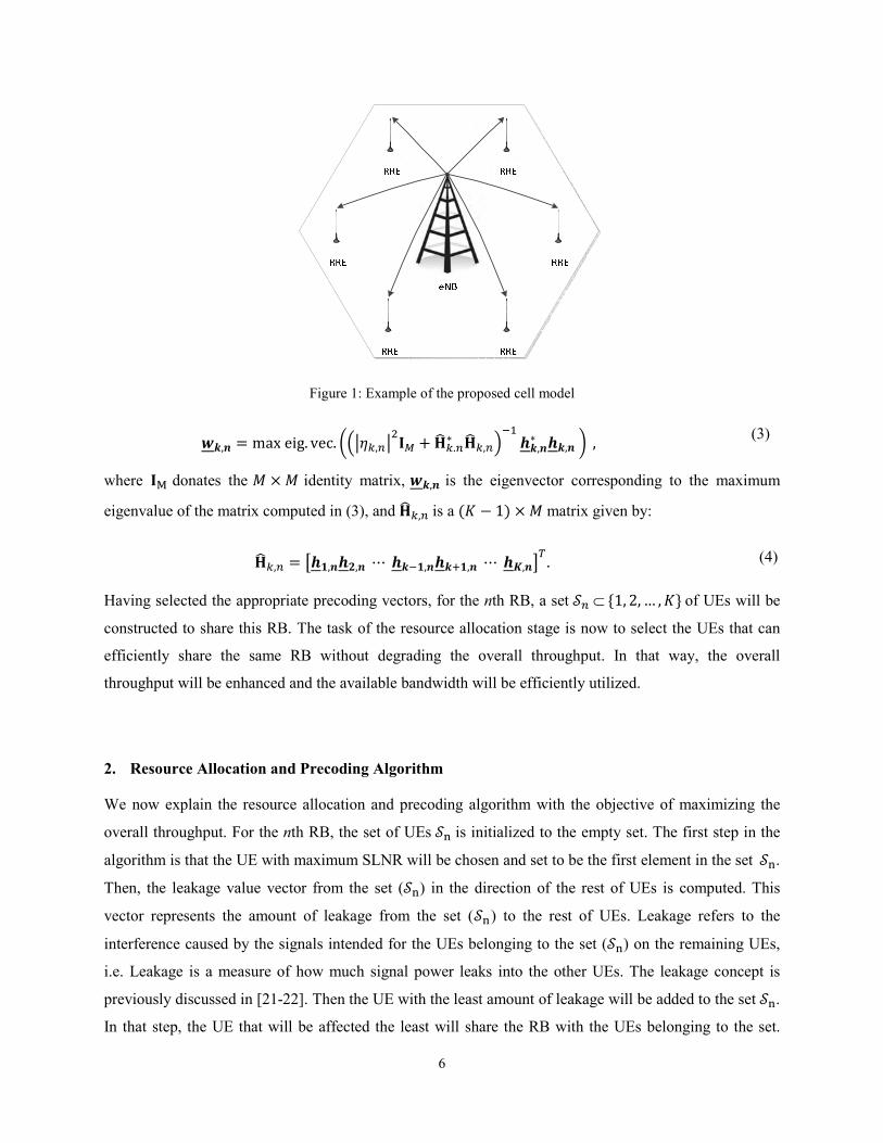
We consider a cellular system where each cell consists of one eNB, M RREs under its control, and serves

K single-antenna UEs. An example of the proposed cell is shown at Fig. 1. There exists N RBs in the

system and each of them may be assigned to serve one or more UEs. The overall transmit power available

5

for each RRE is equal to P. The proposed schemes exploit the SLNR metric for performing the resource

allocation, precoding, and PA. The SLNR (,) at the kth UE over the nth RB can be expressed as:

, = ,,, ∑ ,,, +, , (1)

where , is the power allocated to the kth UE over the nth RB, , is the 1 × complex channel

vector of the links between the kth UE and all M RREs of the CoMP cell, , is the additive white Gaussian noise at the kth UE, and , is an × 1 weighting (precoding) vector that shapes the data

transmitted from the M RREs to the kth UE. The numerator of (1) represents the signal intended for the

kth UE and the first term in the denominator represents the leakage on other UEs due to the signal

intended for the kth UE. It is important to note here, that the weighting vector in the numerator is the same

as the denominator which is not the case for the SINR metric. Thus, selecting each UE weighting vector

based on SLNR is independent of other UEs' weighting vectors, which leads to significant complexity

reduction as will be shown later in the sequel. Moreover, the SLNR metric is function of , and ,which can be obtained by means of time division duplex (TDD) channel reciprocity without the

need of extra channel state information (CSI) feedback.

The choice of the weighting vectors ,, = 1, 2, … , of the UEs will be targeting the maximization

of the SLNR:

Maximize , Subject to, = 1. (2)

In case of the CS scheme, the weighting vector determines which RRE should serve a specific UE. Since

in CS, each UE is served by only one RRE then all the elements in , are zeros except only one element will be equal to unity, which corresponds to the serving RRE. The index of the serving RRE can

be easily obtained by solving the optimization problem in (2) through a simple exhaustive search

procedure. On the other hand, in case of the JP scheme, the same data packet is sent to a specific UE from

all RREs and thus , is not easily obtained as in the case of CS. This optimization problem has been

solved in [23] and the solution was found to be:

6

Figure 1: Example of the proposed cell model

, = maxeig. vec. $%, &' +().∗ (),+,- ,∗ ,. , (3)

where&/ donates the × identity matrix, , is the eigenvector corresponding to the maximum

eigenvalue of the matrix computed in (3), and (),is a ( − 1) × matrix given by:

(), = 34,5, ⋯,4,74, ⋯8,9: . (4)

Having selected the appropriate precoding vectors, for the nth RB, a set ;⊂1, 2, … , of UEs will be constructed to share this RB. The task of the resource allocation stage is now to select the UEs that can

efficiently share the same RB without degrading the overall throughput. In that way, the overall

throughput will be enhanced and the available bandwidth will be efficiently utilized.

2. Resource Allocation and Precoding Algorithm

We now explain the resource allocation and precoding algorithm with the objective of maximizing the

overall throughput. For the nth RB, the set of UEs ;> is initialized to the empty set. The first step in the

algorithm is that the UE with maximum SLNR will be chosen and set to be the first element in the set;>. Then, the leakage value vector from the set (;>) in the direction of the rest of UEs is computed. This

vector represents the amount of leakage from the set (;>) to the rest of UEs. Leakage refers to the interference caused by the signals intended for the UEs belonging to the set (;>) on the remaining UEs,

i.e. Leakage is a measure of how much signal power leaks into the other UEs. The leakage concept is

previously discussed in [21-22]. Then the UE with the least amount of leakage will be added to the set ;>. In that step, the UE that will be affected the least will share the RB with the UEs belonging to the set.

7

This UE will be selected according to [22]. Finally, the algorithm will continue adding UEs to ;> until a certain condition is satisfied (a certain threshold is reached or a certain marginal utility function

with/without look ahead does not increase) as proposed earlier in [22]. It is important to mention that the

resource allocation algorithm achieves a certain level of fairness among UEs as explained in details in

[22].

3. Power Allocation Algorithms

In this section, we investigate three PA algorithms for the CS and JP CoMP schemes, aiming at

minimizing the overall power consumption of the entire network while maximizing the overall data rate.

As mentioned earlier, each RRE has a total power constraint (P) and serves several UEs and each RRE

will initially divide its total power equally over its scheduled UEs.

3.1. Optimal Power Allocation (OPA) Algorithm

The OPA algorithm is designed to deliver high SLNR values for all UEs. This SLNR balancing along

with applying two constraints (per RRE and per RB power constraints) ensure achieving high throughput

gains and reducing the total power consumption at the same time. The OPA algorithm is very complex

due to its coupled nature, however, it can be considered as a benchmark for evaluation to which other

algorithms could be compared. It can also be practically applied in small-scale wireless networks where

the number of available RBs and UEs is considerably small. In contrast, in Sections 4.2 and 4.3, we

propose two algorithms to solve the PA problem in large-scale networks.

We mentioned earlier that each RRE has a total power (P) to be divided among its scheduled UEs, so

each UE has been already allocated a portion of its own serving RRE total power. We consider the

summation of the powers of the UEs belonging to the nth set (the nth set being the set of UEs served over

the nth RB) as the power constraint per the nth RB for the power allocation problem at hand. For

example, if we have three RREs, the first is serving three UEs, the second is serving two UEs, and the

third is serving one UE. Assuming that the nth RB is shared among three UEs (one UE served by each

RRE), and that CS and equal power allocation are used, then the first UE (served by the first RRE) will be

allocated P/3, the second UE will be allocated P/2, and the third one will be allocated P. We can consider

that P/3 + P/2 + P as the power constraint for the nth RB. We can call it the maximum power per RB (?) since the UEs are sharing the same RB. Now, in the above example, we have 1.83P as our per RB

constraint. The proposed power constraint per RB is, in fact, an artificially constructed constraint. Note

8

that, in this example, CS has been assumed, but JP can be applied as well. The allocated power per RB for

a single RRE has been considered before in [26]-[27] where it was required to divide the total power of an

RRE over its allocated RBs. However, the allocated power per RB in case of multiple RREs has not been

used in previous works. The OPA problem can now be formulated as follows:

max@A,B C = D D ,,, ∑ ,,, +, ∈;B,∈;BF

G- , subject to D ,∈;B

≤ ?∀J ∈ 1, 2, … ,K, and D D ,∈LA,M∈NM

≤ P ∀O ∈ 1, 2, … ,, (5)

The optimization problem in (5) is concave since the second derivative of the objective function is non-

negative and the constraints are linear. The solution to the optimization problem defined by (5) (as well

the other problems that will be defined in the sequel) can be found using Newton's method with a

logarithmic barrier penalty, which is one of the interior point methods used for solving convex

optimization problems with inequality constraints [28].

The outline of the Newton with logarithmic barrier method is as follows:

Newton with log barrier Algorithm

Initialize ,, P, μ, RS, RT Repeat

CUTV = (P ∗ C + W) Repeat

Compute Newton step (∆,) and decrement (Ω ) where ∆, = −Z,-[ Ω =[:Z,-[

Compute the step size (η) according to iteration below

While \CUTV\, + ∆,] > CUTV\,] + _ ∗ ∗ [: ∗ ∆,] = ∗

Update , = , + ∗ ∆,

Until Ω ≤ 2RS Update P = μ ∗ P

9

Until F`Babc < RT

In the above algorithm, Wis the barrier function to be added to the objective function C to formulate the

modified objective functionCUTV, KSef is the number of the inequality constraints, RT is the outer desired accuracy (i.e. Accepted tolerance), RS is the inner accuracy. Note that, the desired accuracy of the inner and outer loops can be different. Also, [is the gradient of the modified function, Zis the Hessian of the modified function, and P is a parameter that controls the number of iterations for achieving the desired

accuracy. It is worth noting here, that P is not a fixed parameter, it is a variable parameter that depends on

the iteration number. The barrier function can be found as:

Wg@h(,) = ∑ i− log\? − ∑ ,∈;B ]jFG- +∑ i− log\ − ∑ ∑ ,∈LA,M∈Nm]j'UG-

(6)

It is worth mentioning that the step size (η) is computed via the backtracking line search algorithm [28],

where is a positive constant less than 1 and _is a positive constant less than 0.5. It is also important to

mention that the barrier function in (6) depends on ?, which will be updated in each Newton iteration based on the allocated power for each UE ,. Now, the modified optimization problem will be:

max@A,B Cg@h (7)

where

Cg@h = P ∗ D D ,,, ∑ ,,, +, ∈;B,∈;BF

G- + Wg@h\,]. (8)

In order to solve this optimization problem, we need to get the gradient and the Hessian of (8). The

gradient of the logarithmic barrier function is:

kg@h\Wg@h, ,] =lmnmo 1? − ∑ ,∈;B + 1 − ∑ ∑ ,∈LA,M∈Nm

, CS Scheme

1? − ∑ ,∈;B + D 1 − ∑ ∑ ,∈LA,M∈Nm

'UG- , JP Scheme

(9)

And the gradient of the objective function is:

10

kg@h\C, ,] = ,, (, )[∑ ,,, +, ∈;B, ] . (10)

The Hessian of the logarithmic barrier function is:

Zg@h\Wg@h , S,r , s,t] = D u()\? − ∑ ,∈;B ] F

G- + D v(U)\ − ∑ ∑ ,∈LA,M∈Nm

] ,'

UG- (11)

where

u() = w1, x = y = J0, otherwise , (12)

and

v(U) = w1,x ∈ LS,Uandy ∈ Ls,U0, otherwise . (13)

The Hessian of the objective function can also be found as:

Zg@h\C, ,] = −2 ∗ ,, \, ] ∗ %∑ ,, ∈;B, +∑ ,,, +, ∈;B, | . (14)

Note that the Hessian of the objective function is a diagonal matrix with all entries outside the main

diagonal equal to zero. Based on the above, the gradient and the Hessian of the optimization problem in (7)

are given by:

[g@h = P ∗ kg@h\C, ,] + kg@h\Wg@h, ,], (15)

Zg@h = P ∗ Zg@h\C, ,] + Zg@h\Wg@h, S,r, s,t]. (16)

It is worth noting that the OPA algorithm with the constraints on both the total power per RRE and the

total power per RB turns the optimization problem into a highly coupled one, which is very complicated

and intractable for a large system with a large number of UEs.

We further propose two other relaxed optimization problems; the first one can be solved for each RRE

independently and the second one can be solved for each RB independently. We will use the OPA

algorithm as a benchmark for evaluating the performance of the other two PA algorithms.

11

3.2. Power Allocation per RRE (PAR) Algorithm

Instead of the approach followed by the OPA algorithm, which is based on coupling the multi-cell PA for

all UEs served by all RREs over all RBs at the same time, one may naturally conjecture that solving M

independent (one per RRE) PA optimization problems can provide good system performance while

significantly reducing the computational complexity. When doing so, the power allocation per RRE

(PAR) algorithm can be considered as a sub-optimal but practical algorithm. It attempts to find the power

allocated to each served UE subject to a constraint on the RRE total power. With this assumption, the

optimization problem in (5) will be decoupled and is concave since the power constraint is linear and the

second derivative of the objective function can be shown to be non-negative. The PAR problem can thus

be formulated as:

max@A,B D D ,,, ∑ ,′′′′,, +, ∈;B,∈LA,M∈N~

subjectto D D ,∈LA,M∈N~≤ ∀O ∈ 1, 2, … ,

(17)

The PAR problem is solved for each RRE independently. The solution to this problem can also be found

using Newton with log barrier penalty method as detailed before. We first define the barrier function to be

added to the objective function as:

W@h\,] = D −log − D D ,∈LA,M∈N~'

UG- . (18)

Now, the modified optimization problem will be:

max@A,B C@h

Where(19)

C@h = P ∗ D D ,,, ∑ ,,, +, ∈;B,∈LA,M∈N~+ W@h(,) . (20)

In order to solve this optimization problem, we need to again get the gradient and the Hessian of (20). The

gradient of the logarithmic barrier function is:

12

k@h\Wg@h, ,] =lmnmo 1 − ∑ ∑ ,∈LA,M∈N~ ,CSSchemeD 1 − ∑ ∑ ,∈LA,M∈N~'

UG- ,JPScheme,(21)

and the gradient of the objective function is:

k@h\C, ,] = ,, (, )[∑ ,,, +, ∈;B, ] . (22)

The Hessian of the logarithmic barrier function is:

Z@h\W@h , S,r, s,t] = D v(U)\ − ∑ ∑ ,∈LA,M∈N~ ]

'UG- (23)

where

v(U) = w1,x ∈ LS,Uandy ∈ Ls,U0,otherwise (24)

Finally, the Hessian of the objective function can also be found as:

Z@h\C, ,] = −2 ∗ ,, \, ] ∗ %∑ ,, ∈;B, +[∑ ,,, +, ∈;B, ] (25)

Then the gradient and the Hessian of the optimization problem in (20) are obtained as follows:

[@h = P ∗ k@h\C, ,] + k@h\W@h , ,] (26)

Z@h = P ∗ Z@h\C, ,] + Z@h\W@h , S,r, s,t] (27)

It is assumed that each RRE will have the scheduling decisions of other RREs by means of coordination

(i.e., it will be known to each RRE the sets to which its UEs belong). Although the PAR algorithm is

applied to each RRE independently, it still depends on coordination between RREs. This is because the

SLNR metric couples both the intended signal and the effect on other users in one expression. Hence, if

each RRE considers maximizing the SLNR for only its served UEs, good SINR for all users should be

attainable since other RREs will do exactly the same thing. It is worth noting that the PAR algorithm

controls the signal intended to each UE, but it does not control the interference signal that is resulting

from other UEs sharing the same RB. So, we need to investigate another power allocation algorithm that

13

can control the powers of the UEs sharing the same RB in order to keep the ratio between useful power

and undesired interference below a certain level for all UEs sharing the same RB. This will be the focus

of the next subsection.

3.3. Iterative Power Allocation per RB (IPA) Algorithm

In the iterative power allocation per RB (IPA) algorithm, we consider the UEs belonging to the same set

(sharing the same RB) as the UEs over which the power should be divided. The reasoning behind this is

that the power allocation of each UE within the set affects the whole set in terms of the throughput

(because of the interference caused by any member of the set over the others). Now, if we have N RBs,

we will need to solve the proposed optimization problem N times independently. To do so, we propose

removing the constraint that couples the RBs together (Per-RRE power constraint) in (5). Removing this

constraint ensures transforming the highly coupled optimization problem in (5) into N decoupled

optimization problems. We will show later in the sequel how the per-RRE constraint can be taken into

consideration. To wrap up, the IPA problem has two constraints, but it will be divided into two small

problems, each one of them takes into consideration only one constraint at a time and then we will iterate

over them until we reach a solution. This separation of the constraints with iteration over them can be

considered as a simplified form of the main problem. The optimization problem can now be formulated

as:

max@A,B,∈;B D ,,, ∑ ,′′′′,, +, ∈;B,∈;B,

subjectto D ,∈;B≤ ?∀J ∈ 1, 2, … ,K

(28)

The solution to our problem can now again be found using Newton with log barrier method. We define a

barrier function to be added to the objective function as:

W@h(,) = D−log? − D ,∈;BF

G- (29)

Now, the modified optimization problem will be:

max@A,B C@h (30)

14

whereC@h = P ∗ D ,,, ∑ ,,, +, ∈;B,∈;B

+ W@h(,) (31)

In order to solve this optimization problem, we need to get the gradient and the Hessian of (31). The

gradient of the logarithmic barrier function is:

k@h\W@h, ,] = 1? − ∑ ,∈;B (32)

and the gradient of the objective function is:

k@h\C, ,] = ,, (, )[∑ ,,, +, ∈;B, ] (33)

The Hessian of the logarithmic barrier function is:

Z@h\W@h, S,r, s,t] = D u()\? −∑ ,∈;B ] F

G- (34)

where

u() = w1, x = y = J0,otherwise (35)

The Hessian of the objective function can also be found as:

Z@h\C, ,] = −2 ∗ ,, \, ] ∗ %∑ ,, ∈;B, +[∑ ,,, +, ∈;B, ] (36)

Then the gradient and the Hessian of the optimization problem in (31):

[@h = P ∗ k@h\C, ,] + k@h\W@h, ,] (37)

Z@h = P ∗ Z@h\C, ,] + Z@h\W@h, S,r, s,t] (38)

Now, the first part of the power allocation problem comes to an end here. The objective of the second part

is to reduce the power consumption. Before proceeding further, it is very important to note here that the

power allocation of the first part of the algorithm can lead to an infeasible solution. For example, consider

the same scenario discussed earlier with the three RREs, and let us focus on the second RRE (the one

15

serving two UEs). Assume that it has two available RBs and that after finishing the first part of the

algorithm on the first RB, the UE power allocation was 0.6P, for example, and on the second RB, the UE

power allocation was 0.5P. Now, this RRE should transmit by a total of 1.1P, which is clearly infeasible

as it exceeds the maximum power constraint per RRE. Consequently, the second part of the IPA

algorithm will assure solving the infeasibility problem while reducing the power consumption even

further.

Now, with the aim of reducing the power consumption, the second part of the IPA algorithm will scale the

power allocation vector resulting from the first part without changing the ratios between its elements so

that each element in the vector should never exceed its initial value (the new value should always be less

than the initial). For example, considering the same scenario discussed earlier, the initial power allocation

vector is: = 3 3 2 9 . If the new power allocation vector is, for

example,[0.50.580.75] then it should be updated so that each element does not exceed its

previous value yielding [ 3 0.387 2 ], such that the ratios between the vector elements are the

same. It is clear now that each element does not exceed its previous value leading to a guaranteed feasible

solution and the total power consumption is reduced to 1.22P instead of 1.83P in our example.

After finishing the two parts of the algorithm for all the RBs, we still need to make sure that this

algorithm enhances the overall throughput and also leads to a reduction in the power consumption.

Towards that end, we use the metric defined in [4] and [14], which is the global energy as our stopping

criterion. The global energy is the summation of the inverse of the SINR values of all the UEs sharing the

same RB. If, after each iteration, the new global energy metric is decreased, then this means that the

interference is reduced, leading to improving the throughput and reducing the power consumption. We

then iterate by using the new power allocation vector as the new initial vector (since we are getting better

power allocation vector, it does not make sense to stop until reaching the best one) and we can iterate as

long as the global energy metric is decreasing. In the following subsection, we revisit the IWF algorithm,

which will be used as a benchmark for comparison with our proposed PA algorithms.

3.4. The Iterative water-filling (IWF) Algorithm

For comparison purposes, we apply the iterative water-filling (IWF) algorithm to allocate power to the

UEs sharing the same RB independently. The reason for requiring iterations is that UEs sharing the same

RB interfere with each other. Thus, the power allocated to each UE plays a role in the power allocation of

the rest of the UEs belonging to the same RB group. The IWF concept has been proposed in the context

16

of digital subscriber lines in [24] and was modified in the context of multi user interference management

in [25]-[26].

During IWF iteration, each UE will treat interference from the other UEs as noise. Then, the power

allocated , to the kth UE will be the water-filling solution with noise K and a power constraint of ?: K = D ,,, +,

(39)

Each time , is updated, the interference over each UE (K) and ? will be also updated accordingly. Consequently, the algorithm needs to iterate until it reaches convergence.

4. Computational Complexity Analysis

As shown earlier, in the proposed resource allocation strategies, the weighting vector , is selected in order to maximize the SLNR. Maximizing the SLNR metric (,J) for the kth UE indeed requires less number of computations compared to maximizing the SINR for the same UE. This is because maximizing

the SLNR for each UE is an independent process uncoupled with other UEs. In other words, maximizing

the SLNR for a certain UE requires checking all possible links only for this UE, and no need to check

other UEs links. This is because the SLNR measures the amount of signal power indented for this UE

versus the amount of leakage on other UEs due to that link.

In contrast, maximizing the SINR metric is much more complex process; as the SINR for each UE cannot

be optimized independently. This is because the interference at each UE is dependent on the other UEs

links. Thus, to optimize the SINR for a certain UE, an algorithm should try linking this UE with all

possible links. Also, for each possibility it should try linking other UEs with all possible links.

Consequently, the proposed strategies computational complexity is greatly reduced by considering the

SLNR as the main metric. Also using the SINR would require heavy exchange of information. For

example, the complexity order of maximizing the SINR metric for each UE assuming K UEs and M RREs

and the CS strategy is as follows:

Number of computations in SINR-based resource allocation = '!(',)!, > ( 00)

= ∗ (,-)!(,')! , otherwise

17

This is because in order to maximize the SINR for a specific UE, two stages are needed. The first is to try

linking this specific UE to all RREs in the cell. The second is that while this specific UE is linked with

any RRE, all possible links between the rest of UEs and the rest of RREs should be checked. The number

of computations for the first stage is M in both cases mentioned in (40). However, the number of

computations for the second stage depends on both M and K. When > , the second stage actually will need the same number of computations for selecting − 1 RREs from the available − 1 RREs to serve the − 1 UEs existing in the cell. Moreover, the order of selection should be taken into account.

Consequently, the number of computations for the second stage will be( − 1)-permutations of ( − 1) in case > . When ≥ , the second stage will need the same number of computations for selecting − 1 UEs from the available − 1 UEs to be served by the available − 1 RREs existing in the cell. Moreover, the order of selection should be taken into account. Consequently, the number of computations

for the second stage will equal( − 1)-permutations of( − 1) in case ≥ . By multiplying the

number of computations of both stages and using the basic definition for permutations, (40) can be

obtained.

On the contrary, the complexity of maximizing the SLNR metric for each UE considering the same model

as above is simply of order M. In order to overcome the high computational complexity of maximizing

the SINR at each UE, some papers select the weighting vectors that correspond to the maximum channel

gain, such as in Error! Reference source not found.. However, selecting the weighting vectors in that

way does not take into consideration the interference channels. In contrast, our proposed model

maximizes the SLNR metric for each UE, which checks the interference channels as well as the direct

channel.

5. Performance Evaluation

In this section, the performance of the proposed algorithms will be investigated. It will be shown that the

proposed algorithms significantly outperform the IWF algorithm. In the CS-CoMP case, we consider that

each RRE serves only one UE over the same RB. However, in JP-CoMP, we consider that each UE is

served by all the RREs. We employ the proposed resource allocation and precoding based on SLNR on all

the simulated algorithms. In our simulation, we consider the urban macrocell channel model detailed in

[30] and the UEs to be uniformly distributed over the cell coverage area. The frequency is assumed to be

2 GHz and the subcarrier spacing is 15 KHz. Each RB has 12 subcarriers; we consider different number

of available RBs: 25, 50, 75, and 100 RBs, which correspond to the following system bandwidths: 5, 10,

15, and 20 MHz, respectively. The main simulation parameters are summarized in Table 1.

18

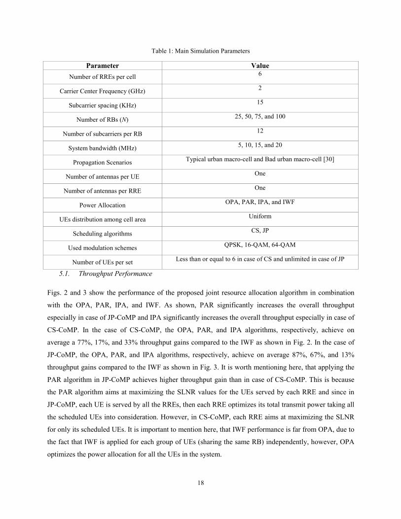
Table 1: Main Simulation Parameters

Parameter Value

Number of RREs per cell 6

Carrier Center Frequency (GHz) 2

Subcarrier spacing (KHz) 15

Number of RBs (N) 25, 50, 75, and 100

Number of subcarriers per RB 12

System bandwidth (MHz) 5, 10, 15, and 20

Propagation Scenarios Typical urban macro-cell and Bad urban macro-cell [30]

Number of antennas per UE One

Number of antennas per RRE One

Power Allocation OPA, PAR, IPA, and IWF

UEs distribution among cell area Uniform

Scheduling algorithms CS, JP

Used modulation schemes QPSK, 16-QAM, 64-QAM

Number of UEs per set Less than or equal to 6 in case of CS and unlimited in case of JP

5.1. Throughput Performance

Figs. 2 and 3 show the performance of the proposed joint resource allocation algorithm in combination

with the OPA, PAR, IPA, and IWF. As shown, PAR significantly increases the overall throughput

especially in case of JP-CoMP and IPA significantly increases the overall throughput especially in case of

CS-CoMP. In the case of CS-CoMP, the OPA, PAR, and IPA algorithms, respectively, achieve on

average a 77%, 17%, and 33% throughput gains compared to the IWF as shown in Fig. 2. In the case of

JP-CoMP, the OPA, PAR, and IPA algorithms, respectively, achieve on average 87%, 67%, and 13%

throughput gains compared to the IWF as shown in Fig. 3. It is worth mentioning here, that applying the

PAR algorithm in JP-CoMP achieves higher throughput gain than in case of CS-CoMP. This is because

the PAR algorithm aims at maximizing the SLNR values for the UEs served by each RRE and since in

JP-CoMP, each UE is served by all the RREs, then each RRE optimizes its total transmit power taking all

the scheduled UEs into consideration. However, in CS-CoMP, each RRE aims at maximizing the SLNR

for only its scheduled UEs. It is important to mention here, that IWF performance is far from OPA, due to

the fact that IWF is applied for each group of UEs (sharing the same RB) independently, however, OPA

optimizes the power allocation for all the UEs in the system.

19

5.2. Power Performance

Fig. 4 shows the normalized average power per RRE. As shown, IWF has the highest power

consumption. This is due to the fact that, IWF does not aim at reducing the power consumption, IWF is

known to use the total power, however, due to the nature of the problem on hand, the power constraint is

not fixed, which may lead to a some power savings. In contrast, the proposed algorithms save a

considerable portion of the power consumed while maintaining the overall throughput considerably high

as shown in Figs. 2 and 3. The OPA, IPA, and PAR algorithms achieve on average a 12%, 7%, and 4%

power reduction compared to IWF and a 14%, 9%, and 6% power reduction compared to the maximum

total power. It is worth mentioning here that the OPA algorithm achieves the best performance in terms of

energy efficiency.

5.3. Convergence and Accuracy

In Fig. 5, we study the desired accuracy versus the number of Newton iterations. As shown, the figure has

a staircase shape where the rise of the stair step represents an outer iteration and the tread of each stair

step represents the number of inner iterations required for that specific outer iteration. As can be shown,

the number of inner iterations decreases with each stair. In other words, the first outer iteration has the

maximum inner iterations, while the last outer iteration has the minimum inner iterations. This is expected

because as the number of outer iterations increases, the output of the previous outer iteration becomes a

very good starting point and the number of Newton steps needed to compute the next outer iteration

becomes small. By means of simulation, it has been found that RT = 10,, RS = 10,, t = 1, andμ = 10, the outer iteration parameter, is optimum in the sense of number of iterations. In Fig. 5, without loss of

generality, we consider N = 100. However, in Fig. 6, we study a measure of the computational effort

where we report the average number of Newton steps versus the number of RBs assuming N = 25, 50, 75

and 100. As can be seen in both figures, OPA has higher computational effort compared to PAR and IPA,

but generally the three algorithms have rapid convergence.

A well-known Hessian approximation is achieved via taking the diagonal parts of the Hessian only and

ignoring the off-diagonal elements to make the inverse Hessian calculations simpler. By applying such

approximation, we show in Fig. 7 that the execution time of the proposed algorithms will definitely be

reduced. The execution time for each algorithm is the time elapsed starting from the Newton's first

iteration until achieving the desired accuracy. It is important to mention here that this plot shows the

normalized execution time. After computing the execution time of each algorithm in both cases (with and

without the Hessian approximation), it is divided by the maximum execution time of all algorithms,

which is OPA with no Hessian approximation when the number of RB’s is equal to 100. Consequently,

20

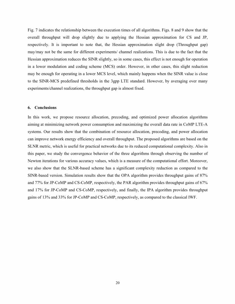
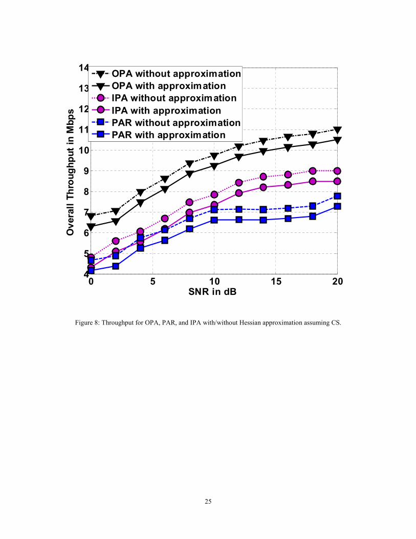
Fig. 7 indicates the relationship between the execution times of all algorithms. Figs. 8 and 9 show that the

overall throughput will drop slightly due to applying the Hessian approximation for CS and JP,

respectively. It is important to note that, the Hessian approximation slight drop (Throughput gap)

may/may not be the same for different experiments/ channel realizations. This is due to the fact that the

Hessian approximation reduces the SINR slightly, so in some cases, this effect is not enough for operation

in a lower modulation and coding scheme (MCS) order. However, in other cases, this slight reduction

may be enough for operating in a lower MCS level, which mainly happens when the SINR value is close

to the SINR-MCS predefined thresholds in the 3gpp LTE standard. However, by averaging over many

experiments/channel realizations, the throughput gap is almost fixed.

6. Conclusions

In this work, we propose resource allocation, precoding, and optimized power allocation algorithms

aiming at minimizing network power consumption and maximizing the overall data rate in CoMP LTE-A

systems. Our results show that the combination of resource allocation, precoding, and power allocation

can improve network energy efficiency and overall throughput. The proposed algorithms are based on the

SLNR metric, which is useful for practical networks due to its reduced computational complexity. Also in

this paper, we study the convergence behavior of the three algorithms through observing the number of

Newton iterations for various accuracy values, which is a measure of the computational effort. Moreover,

we also show that the SLNR-based scheme has a significant complexity reduction as compared to the

SINR-based version. Simulation results show that the OPA algorithm provides throughput gains of 87%

and 77% for JP-CoMP and CS-CoMP, respectively, the PAR algorithm provides throughput gains of 67%

and 17% for JP-CoMP and CS-CoMP, respectively, and finally, the IPA algorithm provides throughput

gains of 13% and 33% for JP-CoMP and CS-CoMP, respectively, as compared to the classical IWF.

21

Figure 2: Overall throughput for OPA, PAR, IPA, and IWF assuming CS

0 5 10 15 204

5

6

7

8

9

10

11

12

SNR in dB

Overall Throughput in Mbps

OPA

IPA

PAR

IWF

22

Figure 3: Overall throughput for OPA, PAR, IPA, and IWF assuming JP.

0 5 10 15 206

8

10

12

14

16

18

SNR in dB

Overall Throughput in Mbps

OPA

PAR

IPA

IWF

23

Figure 4: Normalized average power for OPA, PAR, and IPA.

Figure 5: Desired accuracy versus Newton iterations for OPA, PAR, and IPA.

40 60 80 1000.88

0.9

0.92

0.94

0.96

0.98

1

Number of RB sets

Norm

alized Avera

ge Power

PAR

IPA

IWF

OPA

0 10 20 30 40 5010

-6

10-4

10-2

100

102

104

Newton Iterations

Desired Accura

cy

OPA

PAR

IPA

24

Figure 6: Average number of Newton Steps for OPA, PAR, and IPA.

Figure 7: Normalized Execution time for OPA, PAR, and IPA with/without Hessian approximation

30 40 50 60 70 80 90 10015

20

25

30

35

40

45

Number of RB sets

Avera

ge N

umber of Newto

n Ste

ps

OPA

PAR

IPA

40 60 80 1000

0.2

0.4

0.6

0.8

1

Number of RB sets

Norm

alized Execution tim

e

OPA without approximation

OPA with approximation

IPA without approximation

IPA with approximation

PAR without approximation

PAR with approximation

25

Figure 8: Throughput for OPA, PAR, and IPA with/without Hessian approximation assuming CS.

0 5 10 15 204

5

6

7

8

9

10

11

12

13

14

SNR in dB

Overall Throughput in Mbps

OPA without approximation

OPA with approximation

IPA without approximation

IPA with approximation

PAR without approximation

PAR with approximation

26

Figure 9: Throughput for OPA, PAR, and IPA with/without Hessian approximation assuming JP.

References

[1] 3GPP R1-050833, Interference mitigation in evolved UTRA/UTRAN, LGE Electronics.

[2] Yu, W., Kwon, T., & Shin, C. (2010, March). Joint scheduling and dynamic power spectrum

optimization for wireless multicell networks. In Information Sciences and Systems (CISS), 2010

44th Annual Conference on (pp. 1-6). IEEE.

[3] Parkvall, S., Dahlman, E., Furuskar, A., Jading, Y., Olsson, M., Wänstedt, S., & Zangi, K. C.

(2008, September). LTE-Advanced-Evolving LTE towards IMT-Advanced. In VTC Fall (pp. 1-

5).

[4] Dehghani, M., Arshad, K., & MacKenzie, R. (2014). LTE-Advanced Radio Access

Enhancements: A Survey. Wireless Personal Communications, 1-31.

[5] Irmer, R., Droste, H., Marsch, P., Grieger, M., Fettweis, G., Brueck, S., ... & Jungnickel, V.

(2011). Coordinated multipoint: Concepts, performance, and field trial results. Communications

Magazine, IEEE, 49(2), 102-111.

0 5 10 15 209

10

11

12

13

14

15

16

17

18

19

SNR in dB

Overall Throughput in Mbps

OPA without approximation

OPA with approximation

PAR without approximation

PAR with approximation

IPA without approximation

IPA with approximation

27

[6]

Sawahashi, M., Kishiyama, Y., Morimoto, A., Nishikawa, D., & Tanno, M. (2010). Coordinated

multipoint transmission/reception techniques for LTE-advanced [Coordinated and Distributed

MIMO]. Wireless Communications, IEEE, 17(3), 26-34.

[7] Wang, Q., Jiang, D., Liu, G., & Yan, Z. (2009, September). Coordinated multiple points

transmission for LTE-advanced systems. In Wireless Communications, Networking and Mobile

Computing, 2009. WiCom'09. 5th International Conference on (pp. 1-4). IEEE.

[8] Hosein, P. (2010, May). Coordinated radio resource management for the LTE downlink: The

two-sector case. In Communications (ICC), 2010 IEEE International Conference on (pp. 1-5).

IEEE.

[9] Kiani, S. G., & Gesbert, D. (2008). Optimal and distributed scheduling for multicell capacity

maximization. Wireless Communications, IEEE Transactions on, 7(1), 288-297.

[10] Xu, W., & Liang, L. (2014). On Coordinated Multi-point Transmission with Partial Channel

State Information Via Delayed Feedback. Wireless Personal Communications, 75(4), 2103-

2119.

[11] Kim, B., Malik, S., Moon, S., You, C., Liu, H., Kim, J. H., & Hwang, I. (2014). Performance

Analysis of Coordinated Multi-point with Scheduling and Precoding Schemes in the LTE-A

System. Wireless Personal Communications, 1-16.

[12] Alsharif, M. H., Nordin, R., & Ismail, M. (2013). Classification, Recent Advances and Research

Challenges in Energy Efficient Cellular Networks. Wireless Personal Communications, 1-21.

[13] Hou, X., Bjornson, E., Yang, C., & Bengtsson, M. (2011, September). Cell-grouping based

distributed beamforming and scheduling for multi-cell cooperative transmission. In Personal

Indoor and Mobile Radio Communications (PIMRC), 2011 IEEE 22nd International Symposium

on (pp. 1929-1933). IEEE.

[14] Garcia, V., Chen, C. S., Lebedev, N., & Gorce, J. M. (2011, September). Self-optimized

precoding and power control in cellular networks. In Personal Indoor and Mobile Radio

Communications (PIMRC), 2011 IEEE 22nd International Symposium on (pp. 81-85). IEEE.

[15] Chen, C. S., & Baccelli, F. (2010, May). Self-optimization in mobile cellular networks: Power

control and user association. In Communications (ICC), 2010 IEEE International Conference

on (pp. 1-6). IEEE.

[16] Liu, X., Chong, E. K., & Shroff, N. B. (2002). Joint scheduling and power-allocation for

interference management in wireless networks. In Vehicular Technology Conference, 2002.

Proceedings. VTC 2002-Fall. 2002 IEEE 56th(Vol. 3, pp. 1892-1896). IEEE.

[17] Yu, W., Kwon, T., & Shin, C. (2013). Multicell coordination via joint scheduling, beamforming,

and power spectrum adaptation. Wireless Communications, IEEE Transactions on, 12(7), 1-14.

[18] Gjendemsj, A., Gesbert, D., Oien, G. E., & Kiani, S. G. (2008). Binary power control for sum

rate maximization over multiple interfering links. Wireless Communications, IEEE Transactions

on, 7(8), 3164-3173.

[19] Cho, J. W., Mo, J., & Chong, S. (2009). Joint network-wide opportunistic scheduling and power

28

control in multi-cell networks. Wireless Communications, IEEE Transactions on, 8(3), 1520-

1531.

[20] Venturino, L., Prasad, N., & Wang, X. (2009). Coordinated scheduling and power allocation in

downlink multicell OFDMA networks. Vehicular Technology, IEEE Transactions on, 58(6),

2835-2848.

[21] Abdelaal, R. A., Ismail, M. H., & Elsayed, K. (2012, April). Resource allocation strategies based

on the signal-to-leakage-plus-noise ratio in LTE-A CoMP systems. In Wireless Communications

and Networking Conference (WCNC), 2012 IEEE (pp. 1590-1595). IEEE.

[22] Abdelaal, R. A., Elsayed, K. M., & Ismail, M. H. (2014). Joint Scheduling and Resource

Allocation with Fairness Based on the Signal-to-Leakage-plus-Noise Ratio in the Downlink of

CoMP Systems. Wireless Personal Communications,75(4), 1891-1913.

[23] Sadek, M., Tarighat, A., & Sayed, A. H. (2007). A leakage-based precoding scheme for

downlink multi-user MIMO channels. IEEE Transactions on Wireless Communications, 6(5),

1711-1721.

[24] Yu, W., Ginis, G., & Cioffi, J. M. (2002). Distributed multiuser power control for digital

subscriber lines. Selected Areas in Communications, IEEE Journal on,20(5), 1105-1115.

[25] Yu, W., Rhee, W., Boyd, S., & Cioffi, J. M. (2004). Iterative water-filling for Gaussian vector

multiple-access channels. Information Theory, IEEE Transactions on, 50(1), 145-152.

[26] Yu, W. (2007, January). Multiuser water-filling in the presence of crosstalk. InInformation

Theory and Applications Workshop, 2007 (pp. 414-420). IEEE.

[27] Song, G., & Li, Y. (2003, April). Adaptive subcarrier and power allocation in OFDM based on

maximizing utility. In Vehicular Technology Conference, 2003. VTC 2003-Spring. The 57th

IEEE Semiannual (Vol. 2, pp. 905-909). IEEE.

[28] Boyd, S., & Vandenberghe, L. (2004). Convex Optimization, (Cambridge University Press, 2004).

[29] Batista, R. L., dos Santos, R. B., Maciel, T. F., Freitas, W. C., & Cavalcanti, F. R. P. (2010,

September). Performance evaluation for resource allocation algorithms in CoMP systems.

In Vehicular Technology Conference Fall (VTC 2010-Fall), 2010 IEEE 72nd (pp. 1-5). IEEE.

[30] IST-WINNER II, D1.1.2 (2007). WINNER II Channel Models, 2007, http://www.ist-

winner.org/deliverables.html, accessed January 2015.