Embed Size (px)
Citation preview
Optimization strategies for Markov chain Monte
Carlo inversion of seismic tomographic data.
Dissertation
zur Erlangung des akademischen Grades doctor rerum naturalium(Dr. rer. nat.)
vorgelegt dem Rat der Chemisch-Geowissenschaftlichen Fakultatder Friedrich-Schiller-Universitat Jena
von M.Sc.-Physik, Francesco Fontaninigeboren am 08.11.1983 in Verona (Italien)
Gutachter:
1. Prof. Dr. Florian BleibinhausLehrstuhl fur Angewandte GeophysikMontanuniversitat Leoben
2. Prof. Dr. Michael KornLehrstuhl fur Teoretische GeophysikUniversitat Leipzig
Tag der Verteidigung: 04.07.2016
Contents
Contents i
Abstract v
Zusammenfassung vii
List of Figures xiii
List of Tables xv
List of Abbreviations xvii
1 Bayesian inference and McMC methods. 11.1 Deterministic VS probabilistic approach to inverse problems. . . . . 11.2 Probabilistic methods in geophysics: state of the research . . . . . . 21.3 Computational cost and optimization strategies. . . . . . . . . . . . 3
1.3.1 Forward modeling . . . . . . . . . . . . . . . . . . . . . . . . 31.3.2 Model Parametrization . . . . . . . . . . . . . . . . . . . . . 41.3.3 Optimized updating schemes . . . . . . . . . . . . . . . . . . 51.3.4 Parallelization of Markov processes . . . . . . . . . . . . . . 5
1.4 McMC within Simulr16 . . . . . . . . . . . . . . . . . . . . . . . . 61.5 Statistical inference: from integration to Markov chain Monte Carlo 81.6 Fundamental properties of Markov Chains . . . . . . . . . . . . . . 9
1.6.1 Markov Chain . . . . . . . . . . . . . . . . . . . . . . . . . . 91.6.2 Ergodicity and Stationarity . . . . . . . . . . . . . . . . . . 111.6.3 Reversibility . . . . . . . . . . . . . . . . . . . . . . . . . . . 14
1.7 Markov chain Monte Carlo . . . . . . . . . . . . . . . . . . . . . . . 141.7.1 Bayesian inference . . . . . . . . . . . . . . . . . . . . . . . 15
1.7.1.1 Inverse problem . . . . . . . . . . . . . . . . . . . . 151.7.1.2 Probability . . . . . . . . . . . . . . . . . . . . . . 171.7.1.3 Bayes’ theorem . . . . . . . . . . . . . . . . . . . . 17
1.7.2 Metropolis-Hastings algorithm . . . . . . . . . . . . . . . . . 18
i

Contents
1.7.3 Transdimensional McMC . . . . . . . . . . . . . . . . . . . . 211.7.4 The likelihood function . . . . . . . . . . . . . . . . . . . . . 211.7.5 Analyzing the esemble properties . . . . . . . . . . . . . . . 22
2 Transdimensional McMC 252.1 Reversible jump McMC . . . . . . . . . . . . . . . . . . . . . . . . . 252.2 Method: Bayesian traveltime tomography . . . . . . . . . . . . . . . 25
2.2.1 Prior distributions . . . . . . . . . . . . . . . . . . . . . . . 252.2.2 Proposals: how to move between models. . . . . . . . . . . . 272.2.3 Transdimensional acceptance ratios . . . . . . . . . . . . . . 292.2.4 Updating scheme . . . . . . . . . . . . . . . . . . . . . . . . 30
2.3 Synthetic dataset . . . . . . . . . . . . . . . . . . . . . . . . . . . . 312.3.1 Multiple Parallel Markov Chains . . . . . . . . . . . . . . . 322.3.2 Staggered grids . . . . . . . . . . . . . . . . . . . . . . . . . 332.3.3 Burn-in and convergence estimation . . . . . . . . . . . . . . 352.3.4 Inversion . . . . . . . . . . . . . . . . . . . . . . . . . . . . . 37
2.3.4.1 Posterior distributions PDF . . . . . . . . . . . . . 382.3.4.2 Mean and Modal solutions . . . . . . . . . . . . . . 402.3.4.3 Uncertainty map . . . . . . . . . . . . . . . . . . . 41
2.4 Salzach valley . . . . . . . . . . . . . . . . . . . . . . . . . . . . . . 432.4.1 Transdimensional McMC inversion results . . . . . . . . . . 44
2.4.1.1 Posterior distributions . . . . . . . . . . . . . . . . 482.4.1.2 Transdimensional inversion results . . . . . . . . . 492.4.1.3 Error maps . . . . . . . . . . . . . . . . . . . . . . 51
2.5 Conclusions . . . . . . . . . . . . . . . . . . . . . . . . . . . . . . . 53
3 Resolution Matrix for a Multivariate updating scheme 553.1 Introduction . . . . . . . . . . . . . . . . . . . . . . . . . . . . . . . 55
3.1.1 Optimization of Metropolis-Hastings McMC . . . . . . . . . 563.1.2 Comparing the efficiency of Markov Chains . . . . . . . . . . 573.1.3 Model Resolution Matrix . . . . . . . . . . . . . . . . . . . . 59
3.2 Method . . . . . . . . . . . . . . . . . . . . . . . . . . . . . . . . . 613.2.1 Test model . . . . . . . . . . . . . . . . . . . . . . . . . . . 613.2.2 Deterministic inversion . . . . . . . . . . . . . . . . . . . . . 623.2.3 Prior . . . . . . . . . . . . . . . . . . . . . . . . . . . . . . . 633.2.4 Proposal and updating scheme . . . . . . . . . . . . . . . . . 643.2.5 Perturbation scaling . . . . . . . . . . . . . . . . . . . . . . 663.2.6 Algorithm implementation . . . . . . . . . . . . . . . . . . . 67
3.2.6.1 Full-ResM updating scheme . . . . . . . . . . . . . 683.2.6.2 Fix-ResM updating scheme . . . . . . . . . . . . . 72
3.3 Tests and results . . . . . . . . . . . . . . . . . . . . . . . . . . . . 75
ii

Contents
3.3.1 Non-McMC tests . . . . . . . . . . . . . . . . . . . . . . . . 763.3.2 Fix-ResM McMC test . . . . . . . . . . . . . . . . . . . . . 813.3.3 Bayesian seismic tomography with the Fix-ResM McMC al-
gorithm . . . . . . . . . . . . . . . . . . . . . . . . . . . . . 873.3.3.1 Ensemble properties . . . . . . . . . . . . . . . . . 88
3.4 Discussion and Conclusions . . . . . . . . . . . . . . . . . . . . . . 90
4 Discussion and conclusions 914.1 Achievements . . . . . . . . . . . . . . . . . . . . . . . . . . . . . . 914.2 Future directions . . . . . . . . . . . . . . . . . . . . . . . . . . . . 92
4.2.1 Voronoi parametrization . . . . . . . . . . . . . . . . . . . . 924.2.2 Reflection-refraction seismics . . . . . . . . . . . . . . . . . . 934.2.3 Combined functionals . . . . . . . . . . . . . . . . . . . . . . 944.2.4 Transdimensional McMC and Resolution Matrix . . . . . . . 944.2.5 A unified approach . . . . . . . . . . . . . . . . . . . . . . . 95
Bibliography 102
Acknowledgements 103
Selbstandigkeitserklarung 105
Curriculum Vitae 107
iii

Contents
iv
Abstract
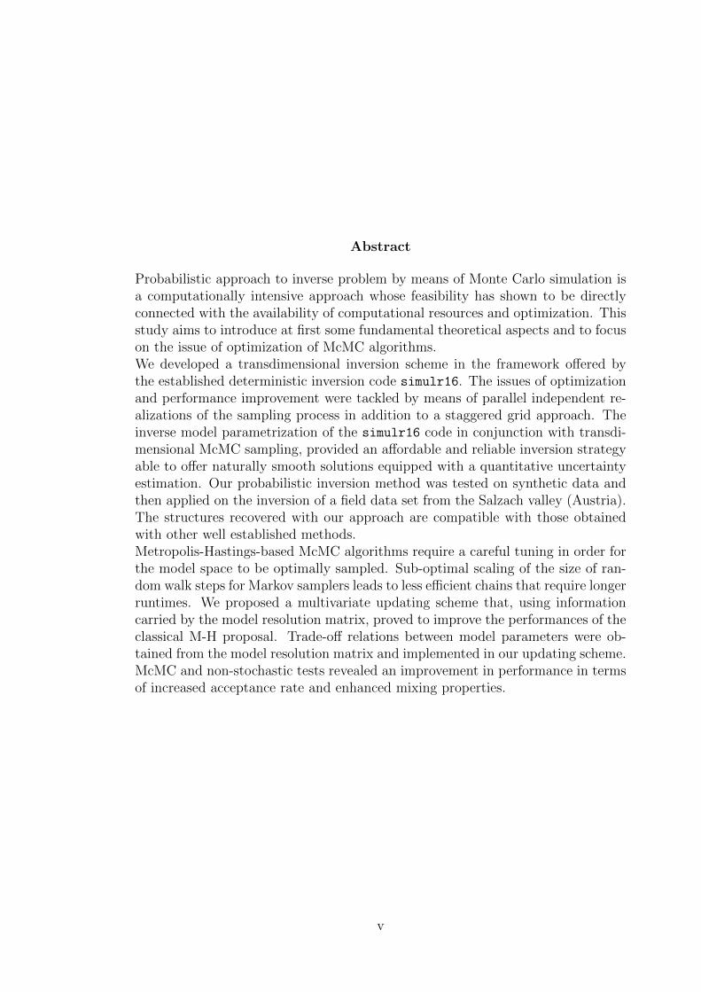
Probabilistic approach to inverse problem by means of Monte Carlo simulation isa computationally intensive approach whose feasibility has shown to be directlyconnected with the availability of computational resources and optimization. Thisstudy aims to introduce at first some fundamental theoretical aspects and to focuson the issue of optimization of McMC algorithms.We developed a transdimensional inversion scheme in the framework offered bythe established deterministic inversion code simulr16. The issues of optimizationand performance improvement were tackled by means of parallel independent re-alizations of the sampling process in addition to a staggered grid approach. Theinverse model parametrization of the simulr16 code in conjunction with transdi-mensional McMC sampling, provided an affordable and reliable inversion strategyable to offer naturally smooth solutions equipped with a quantitative uncertaintyestimation. Our probabilistic inversion method was tested on synthetic data andthen applied on the inversion of a field data set from the Salzach valley (Austria).The structures recovered with our approach are compatible with those obtainedwith other well established methods.Metropolis-Hastings-based McMC algorithms require a careful tuning in order forthe model space to be optimally sampled. Sub-optimal scaling of the size of ran-dom walk steps for Markov samplers leads to less efficient chains that require longerruntimes. We proposed a multivariate updating scheme that, using informationcarried by the model resolution matrix, proved to improve the performances of theclassical M-H proposal. Trade-off relations between model parameters were ob-tained from the model resolution matrix and implemented in our updating scheme.McMC and non-stochastic tests revealed an improvement in performance in termsof increased acceptance rate and enhanced mixing properties.
v

Contents
vi
Zusammenfassung
Der probabilistische Ansatz fur die Losung des Inversionproblems unter Verwen-dung der Monte Carlo Simulation ist ein sehr rechenintensiver Ansatz dessen Um-setzbarkeit direkt mit den verfugbaren rechentechnischen Ressourcen verbundenist. Die Absicht dieser Studie ist zuerst einige fundamentale theoretische Aspektedarzustellen und anschlieend das Problem der Optimierung von McMC Algorith-men zu erlautern.Wir entwickelten ein mehrdimensionales Inversionsschema welches in den bere-its vorhandenen deterministischen Inversionscode simulr16 integriert wurde. DasProblem der Optimierung und Verbesserung der Leistungsfahigkeit wurde bewaltigtunter Verwendung von parallelen unabhangigen Modelprobenketten und des stag-gered grid Ansatzes. Die Parametrisierung des Inversionsmodells im simulr16Code in Verbindung mit der mehrdimensionalen McMC Probenkette ermoglichteine erschwingliche und zuverlassliche Inversionsstrategie welche naturlich glatteLosungen mit einer zusatzlichen quantitativen Unsicherheitsbestimmung bereit-stellt. Unsere probabilistische Inversionsmethode wurde an synthetischen Datengetestet und anschlieend auf den realen Datensatz des Salzach Tals (osterreich)angewendet. Die mit unserer Methode aufgelosten Strukturen sind vergleichbarmit Denen von anderen bereits integrierten Inversionsmethoden.Metroplolis-Hasting basierende McMC Algorithmen benotigen eine sorgfaltige An-passung, damit der Modelraum optimal abgetastet wird. Eine suboptimale Skalierungder Groe der zufalligen Laufschritte fur Markov-Sampler fuhrt zu geringer ef-fizienten Ketten, welche langere Laufzeiten benotigen. Zur Verbesserung der Leis-tungsfahigkeit von klassischen M-H-Ansatzen schlagen wir ein multivariates Update-Schema vor, dass die Informationen der Modell-Auflosungsmatrix nutzt. Die Aus-tauschbeziehung zwischen den Modellparametern wird durch die Auflosungsma-trix bereitgestellt und wurde in unserem Update-Schema implementiert. McMCund Non-stochastische Tests zeigen eine Verbesserung in der Leistungsfahigkeit imSinne von ansteigender Akzeptierungsrate und erhohter Mischeigenschaft.
vii

Contents
viii

List of Figures
1.1 Summary of the properties, and their interrelationships, of the Markovchains involved in this study. Such properties are granted by tran-sition kernels provided by the Metropolis-Hastings algorithm. . . . . 15
2.1 Iterative updating scheme of our transdimensional McMC algorithm. 302.2 The synthetic model used in this chapter: (a) the main structural
features are here tagged as A1,A2 (low velocity anomalies) L1,L2(layers). (b) Receiver locations (triangles) and ray paths for threeof the sources (stars). . . . . . . . . . . . . . . . . . . . . . . . . . . 31
2.3 Speedup relations for a multiple chains approach showing the the-oretical linear speedup (black) in case of no burn-in (perfect paral-lelization), the curve (red) for an hypothetical case where the initial10% of the models is discarded and the curve (green) for the 0.5%-burn-in we obtained in the inversion of the Salzach dataset (seesection 2.4) . . . . . . . . . . . . . . . . . . . . . . . . . . . . . . . 32
2.4 Staggered grids: the original grid is shifted in four directions. . . . . 332.5 Conditional probability density functions comparison: the same
model is parametrized with a coarse node parametrization (a) andwith a 5 times finer node spacing (b) and (c). The probability dis-tributions are plotted at the same profile position only at depthswhere a node is present. The PDF in (a) and (b) are plotted after105 iterations, while in (c) after 106. . . . . . . . . . . . . . . . . . . 34
2.6 Temporal evolution of the normalized misfits for five instances ofstaggered chains . . . . . . . . . . . . . . . . . . . . . . . . . . . . . 35
2.7 Temporal evolution of normalized misfit values of the first 5000models saved in two different Markov chains. (a) the chain initial-ized with a random model-state needs to have the first part of themodels rejected (burn-in phase highlighted in the cyan box). (b)Having initialized the sampling process with the DLS solution noburn-in is necessary. . . . . . . . . . . . . . . . . . . . . . . . . . . 35
ix

List of Figures
2.8 Likelihood PDFs : probability distribution of the likelihood valuesof a Markov chain for (cyan) all models proposed, (green) acceptedmodels, (red) rejected models. . . . . . . . . . . . . . . . . . . . . . 36
2.9 Deterministic solution model used to initialize the Markov Chain.Isolines of the synthetic model are reported for comparison as a reddashed curve. Inversion nodes are marked with crosses. . . . . . . . 37
2.10 RDE map: Resolution Diagonal Elements . . . . . . . . . . . . . . 37
2.11 Locations of the PDF vertical cross sections on the model: solidblue lines. . . . . . . . . . . . . . . . . . . . . . . . . . . . . . . . . 38
2.12 continues on next page . . . . . . . . . . . . . . . . . . . . . . . . . 38
2.13 Mean model solutions compared: single Markov chain (top) multiplestaggered chains (bottom). The red-dashed isolines are relative tothe synthetic model while the black ones to the mean solutions. . . 40
2.14 Modal velocity model corresponding to the multiple-staggered Markovchain. . . . . . . . . . . . . . . . . . . . . . . . . . . . . . . . . . . 41
2.15 Standard deviation map with contour lines of the synthetic structure. 42
2.16 Quantitative error maps: standard error (top) and relative error(bottom). The dashed contour lines display for comparison thesynthetic structure. . . . . . . . . . . . . . . . . . . . . . . . . . . . 42
2.17 Map of the Salzach river valley (left), the inset maps the investiga-tion area. Seismic profile with shot locations (circles) and receivers(red line). . . . . . . . . . . . . . . . . . . . . . . . . . . . . . . . . 43
2.18 Deterministic DLS solutions obtained inverting refraction-reflectiondata (a) and first arrivals only (b). The RRTT solution of Bleib-inhaus and Hilberg (2012) is reported on the left (a) together withthe node parametrization used for the inversion (crosses), reflectorparameters (circles) and the explosive sources (stars). On the right(b) the FATT solution used in this study as starting model for theMcMC process. . . . . . . . . . . . . . . . . . . . . . . . . . . . . . 44
2.19 Log-likelihood traces of the initial part for the 9 staggered chains. Inthe legend the sketch represents the shift direction of the staggeredgrids for each chain and the corresponding color of the traces. . . . 45
2.20 continues on next page . . . . . . . . . . . . . . . . . . . . . . . . . 46
2.21 Posterior distribution on the number of inverse parameters for theensemble. The modal value corresponds to 33 nodes. . . . . . . . . 48
x

List of Figures
2.22 Solution models compared: transdimensional McMC mean model(a), deterministic Full Waveform Inversion (b), deterministic Reflection-Refraction (c), deterministic first arrivals staggered (d). The arrowsrefer to features recovered with different methods, discussed in thetext. . . . . . . . . . . . . . . . . . . . . . . . . . . . . . . . . . . . 50
2.23 Standard deviation (a) and relative error (b) maps. . . . . . . . . . 51
2.24 Node recurrence map: the positions of possible inversion nodes(crosses) are displayed together with the relative frequency of eachnode being considered as an inverse parameter. Nodes that weremore often set as inversion parameters have colors tending towardsgreen, conversely less-often inverted nodes display colors towards red. 52
3.1 A graphical representation of equation 3.8 relating a synthetic seis-mic velocity model (right) to one possible DLS-solution (left) throughthe model resolution matrix (middle). The ith row of R shows howa perturbation of the true synthetic model will be mapped into theinverse parameters of mest. Well resolved inverse parameters havehigher diagonal-element values (Rii ≈ 1, darker colors), poorly re-solved parameters with almost zero resolution will tend to white. . . 60
3.2 Synthetic model with ray paths relative to the sources 1, 12, 23(star). The receivers positions are marked with a triangle. . . . . . 61
3.3 a) Deterministic DLS solution: the dashed-black lines are contourlines of the synthetic model for the velocity values 1.5 and 3 Km/s.b) RDE map of the model solution above: the Resolution DiagonalElements were used to optimize the distribution of nodes (blackcrosses) . . . . . . . . . . . . . . . . . . . . . . . . . . . . . . . . . 63
3.4 Prior information: velocity ranges are defined both on the surfaceand on the bottom of the model to obtain the prior at each depththrough linear interpolation. . . . . . . . . . . . . . . . . . . . . . . 64
3.5 Example: a perturbation to the 5th model parameter (big +) isbalanced by opposite-sign compensations. The global biasing effectof a perturbation on the model is thus reduced, resulting in a modelthat is more likely to be accepted. . . . . . . . . . . . . . . . . . . . 66
3.6 Depth dependent perturbation size defined as a fraction of the priorrange. . . . . . . . . . . . . . . . . . . . . . . . . . . . . . . . . . . 66
3.7 Table reporting the node depths and the corresponding prior ve-locity intervals together with the standard deviation of the randomperturbations. . . . . . . . . . . . . . . . . . . . . . . . . . . . . . . 67
xi

List of Figures
3.8 Acceptance rate / k-factor relations: the selected value for the per-turbation scaling factor is k = 0.1 and corresponds to 1/10 of thevelocity prior. The green area marks the optimal range character-ized by a 20− 30% acceptance rate. . . . . . . . . . . . . . . . . . . 67
3.9 Scheme of the Full-ResM McMC algorithm: this updating schemeincludes the computation of the resolution matrix at every iterationof the Markov process. . . . . . . . . . . . . . . . . . . . . . . . . . 69
3.10 Posterior distributions of the velocity displayed for profile position25 (a) and 60 (b) obtained with the Full-ResM updating scheme.The area delimited by the dashed red curves corresponds to the prior. 70
3.11 Scheme of the Fix-ResM McMC algorithm: the steps grouped inthe light blue box constitute the iterative McMC process, whereasthe first three points are part of the deterministic initialization ofthe inversion. . . . . . . . . . . . . . . . . . . . . . . . . . . . . . . 74
3.12 Misfit analysis: percentage of models with a reduced misfit after aperturbation for five perturbation schemes (classical M-H no-ResMand 4 ResM functionals). Shallow, middle and deep sets of nodeshave been analyzed separately. . . . . . . . . . . . . . . . . . . . . . 78
3.13 Depth-based subdivision of the nodes in the model in three groups:shallow (green) , middle (yellow), and deep (red). The dashed linesare contour lines (as in Fig.3.3.a) reported as a reference for thesynthetic structure. . . . . . . . . . . . . . . . . . . . . . . . . . . . 79
3.14 LD-distributions produced by the four functional under exam com-pared with the distribution obtained with the no-ResM functional(in red). A better-performing algorithm is expected to produce arightwards-shifted LD-distribution, with a higher recurrence for val-ues around zero. . . . . . . . . . . . . . . . . . . . . . . . . . . . . . 80
3.15 Comparison of the LD-distributions of Markov chains based on theFix-ResM updating scheme. In red the reference distribution rela-tive to the “classical” McMC. . . . . . . . . . . . . . . . . . . . . . 82
3.16 McMC traces of two parameters corresponding to nodes at depthsof respectively 0.1 and 25 m. The P-velocity is plotted for everyMcMC iteration in the range [1000, 4000]. The amount and fre-quency of velocity changes provide a qualitative estimation of themixing properties of each algorithm. The difference is especiallystrong for the uppermost parameters, here it’s clear that the use ofour FIX-ResM updating scheme (green traces on the right) resultsin a more frequent update of the velocity value. . . . . . . . . . . . 84
xii

List of Figures
3.17 Variance difference maps between the four functionals and the NoResMMcMC. Functional-a is the only that displays only a variance reduc-tion. . . . . . . . . . . . . . . . . . . . . . . . . . . . . . . . . . . . 86
3.18 Vertical cross sections of the posterior distribution at profile posi-tion 25 and 60 m. displayed together with the mean model, DLSdeterministic solution and synthetic “real” values. The thin pinklines mark the confidence interval given by ± one standard deviation. 87
3.19 Mean model: the dashed black line represents the isolines corre-sponding to p-wave velocities of 1.5 and 3.0 Km/s of the extractedmean-mode solution, the red dashed reports for comparison thesame isolines for the test synthetic model. . . . . . . . . . . . . . . 88
3.20 Standard deviation map obtained from the posterior probability dis-tribution (a) and map of the resolution diagonal elements obtainedfrom the last iteration of the DLS solution (b). For the resolutionmap, the contour lines are defined basing on the node subdivisionof Pag.77. . . . . . . . . . . . . . . . . . . . . . . . . . . . . . . . . 89
3.21 Relative error map: the black dashed line marks the contours of10% relative standard error, the red contours report for comparisonthe main structural features of the synthetic model. . . . . . . . . . 90
xiii

List of Figures
xiv

List of Tables
2.4.1 Inversion data recap . . . . . . . . . . . . . . . . . . . . . . . . . . 45
3.3.1 Acceptance rates [%] relative to Markov chains characterized by theuse of the four functionals plus the “classical” non-ResM McMC. . . 81
3.3.2 Evaluations of eq. 3.31 computed for each functional. . . . . . . . . 853.4.1 Performance comparison between a classical M-H McMC and our
Fix-ResM algorithm. . . . . . . . . . . . . . . . . . . . . . . . . . . 90
xv

List of Tables
xvi

List of Abbreviations
PDF . . . . . . . . . . Probability Density Function
McMC . . . . . . . Markov chain Monte Carlo
rj-McMC . . . . . reversible jump Markov chain Monte Carlo
ART-PB . . . . . Approximate Ray Tracing Pseudo ray Bending
ResM . . . . . . . . . Resolution Matrix
RDE . . . . . . . . . . Resolution Diagonal Elements
gcd . . . . . . . . . . . greatest common divisor
iid . . . . . . . . . . . . independent identically distributed
CLT . . . . . . . . . . Central Limit Theorem
M-H . . . . . . . . . . Metropolis-Hastings
LSQR . . . . . . . . Least Squares
DLS . . . . . . . . . . Damped Least Squares
FATT . . . . . . . . . First Arrival Traveltime tomography
RRTT . . . . . . . . Refraction-Reflection Traveltime tomography
FWI . . . . . . . . . . Full Waveform Inversion
LD . . . . . . . . . . . . Likelihood differences
xvii

List of Tables
xviii
Chapter 1
Bayesian inference and McMCmethods: a probabilistic approachto inverse problems in geophysics.
1.1 Deterministic VS probabilistic
approach to inverse problems.
Seismic traveltime tomography is, together with other inverse problems in geo-physics, often approached through iterative linearized techniques which simplify anon-linear physical reality while aiming to obtain an optimum solution, a singlemodel, found avoiding local minima by means of regularization.
This deterministic approach to the inversion of traveltimes in seismic tomographycarries many of the sources of uncertainty and instability that generally charac-terize inverse problems. Uneven coverage, limited quality of the data, inadequateparametrization, and non-uniqueness of solutions, are within the most notable.Regularization techniques are employed in the attempt to avoid local minima, ad-hoc optimized parameterizations are used but nonetheless the null space remainsunknown and the single-model solution generally proposed does not reflect theintrinsic non-uniqueness of the inverse problem. Providing constraints on the un-certainty is therefore a major issue, some of the most widely adopted methodsinclude the evaluation of ray path densities, null-space energy, resolution matrixdiagonal elements, and other estimators that provide a qualitative estimation ofthe uncertainty and on the interdependency of the inverse parameters. A qual-itative map of the spatial resolving power of a data set is often obtained withcheckerboard tests. A mayor downside of these tests and methods is connectedwith the intrinsic nature of the deterministic solution they are probing: they arelocal. No global overview of all the possible solutions and respective uncertain-
1

1.2. Probabilistic methods in geophysics: state of the research
ties can be achieved through inverse methods that linearize non-linear physicalsystems. Despite the mentioned limitations the approach to inverse problems ingeophysics is mainly deterministic; still valuable information and interpretationresults are proposed and positively utilized.
In contrast to the previous methods, the probabilistic, or Bayesian, approach toseismic tomographic problems is a fully non-linear approach. All the knowledge onthe physical objects under study is conveyed in terms of probabilities, the wholemodel space is analyzed with the positive outcome that local minima aren’t dis-regarded in the quest for a solution, on the contrary the probabilistic approachprovides a global overview on the values of the model parameters together withtheir relative uncertainties. This results in the possibility to quantitatively esti-mate the non-uniqueness of the problem in terms of probability density functionsand to obtain not a single solution but global inference from a stochastic ensem-ble. Bayesian theory joins a priori information that we have before performingmeasurements, with the ability of different sets of model parameters to fit themeasured data (likelihood), in order to obtain a conditional probability densityfunction (PDF) in the model space, referred as posterior distribution.
The probabilistic approach to inverse problems offers a further advantage: the pos-sibility to treat the number of model parameters as an unknown in the inversionprocess allowing the data to drive the parametrization. This achievement seemsto remove that source of uncertainty given by the necessary choice or estimationof many inversion parameters. The task to define number and distribution ofparameters as well as damping and smoothing is in this way passed to the dataitself, reducing the possible error sources due to this potentially subjective choice.Nonetheless, depending on the way specific algorithms are implemented, other dif-ferent parameters might be introduced in the inversion process, which are also inneed of a correct estimation. See for instance the treatise of Bodin et al. (2012)of unknown data noise as an hyperparameter in rj-McMC. Adaptive and irregularparametrization strategies are however established also in the deterministic frame-work (see section 1.3.2), together with methods and workflows to assess optimalvalues for some inversion parameters.
1.2 Probabilistic methods in geophysics:
state of the research
The development of probabilistic algorithms is strongly linked to the developmentof fast computing machines. It was pioneered by Metropolis et al. (1953), whodeveloped and applied a Markov Chain algorithm to investigate the Boltzmanndistribution. His approach was generalized a few years later by Hastings (1970).
2

Chapter 1. Bayesian inference and McMC methods.
First geophysical applications of probabilistic methods to inverse problems werereported by Press (1968), Keilis-Borok and Yanovskaja (1967), and during the fol-lowing decades, Monte Carlo methods became an established inversion approachfor small geophysical problems. Geophysical applications of Bayesian inferenceare described in Tarantola and Valette (1982), Duijndam (1988a,b), Mosegaardand Tarantola (1995). A brief overview of the early applications and the develop-ment of probabilistic techniques are given in the review paper of Sambridge andMosegaard (2002). Today, probabilistic methods are well established for the 1Dinversion of body wave traveltimes (Sambridge and Mosegaard, 2002), and are alsowidely used for the 1D inversion of surface wave dispersion curves at a broad rangeof scales (Shapiro and Ritzwoller, 2002; Socco and Boiero, 2008). As Mosegaardand Tarantola (1995) point out, Markov chains alone may not suffice to cope withrealistic geophysical problems, because the acceptance rate of randomly perturbedmodels can be so low that the problem becomes computationally intractable. Thestrategy is to restrict the application of the forward solution so far as possible to therelevant models with the practice of importance sampling (Mosegaard, 1998). Acommon approach is the Markov chain Monte Carlo (McMC) method, mostly im-plemented through the Metropolis-Hastings algorithm. The problem of the modelparametrization has been addressed in a transdimensional framework mostly withthe reversible-jump algorithm by Green (1995); Green and Mira (2001) (Sambridgeet al., 2006; Gallagher et al., 2009). Most of the published works employing rj-McMC algorithms lie in the genetics field. Bodin et al. (2012) implemented aself-parametrized data noise treatment as an extension of their delayed-rejection,reversible-jump algorithm (Bodin and Sambridge, 2009).
1.3 Computational cost
and optimization strategies.
Markov chain and McMC methods are extremely computationally-intensive al-gorithms which generally require computation times that reach some order ofmagnitude more than their deterministic equivalent. For this reason a numberof strategies must be considered in order to contain the computational time. Inthe following sections a brief overview is presented on the most commonly adoptedstrategies.
1.3.1 Forward modeling
The solution of the forward problem is often the part of the inversion processthat absorbs most of the CPU time. Seismic tomography problem are not anexception and the optimization of the forward routines is fundamental to avoid
3

1.3. Computational cost and optimization strategies.
wasting computational resources. In the framework of the software package weare developing, a choice is given to the user on the forward computation strategyto adopt: either a bending ray tracer combined with a grid search of Bleibinhaus(2003) after Um and Thurber (1987)or a finite-differencies-eikonal solver of Vidale(1990) with modifications of Hole (1992). In this work the latter will be alwaysemployed to solve the forward problem. The CPU time spent in the computa-tion of the time-field is directly proportional to the number of seismic sources; atest performed on a synthetic dataset (see section 2.3) characterized by 23 sourcesshows that forward computation through the eikonal solver takes over 90% of thetime needed to perform an iteration. Parallelization of the forward routines overthe sources is therefore a valid approach that promises a reduction of the comput-ing time almost proportional to the number of CPUs/cores utilized. Additionalstrategies intended to reduce the forward time-cost have been developed and theyinclude emulations and approximations of the forward modeling. Debski (2010)for instance simply uses straight ray paths for a 2D inversion of body waves whileBodin and Sambridge (2009) use great-circle paths for the 2D inversion of sur-face wave group velocity for Australia. Such simplifications can be justified, ifthe actual rays are close to those paths, and if moderate velocity perturbationscause only minor ray path deviations. In general, approximate forward modelingis acceptable in a probabilistic framework (Koutsourelakis, 2009).
1.3.2 Model Parametrization
The computational load of probabilistic methods can be reduced limiting the num-ber of the inverse variables that parametrize a certain model. A number of studiesdeal with methods to adapt the inverse grid, employing irregular parametrizationschemes aiming to match the resolving power of the data. Different strategieshave been proposed and applied to seismic inverse problems by, e.g., Sambridgeet al. (1995), Thurber and Eberhart-Phillips (1999), Bohm et al. (2000), Bleib-inhaus (2003), Trinks et al. (2005), Ajo-Franklin et al. (2006), Bleibinhaus andGebrande (2006) and Bodin and Sambridge (2009). In our work in Chap.2 we willadopt a transdimensional approach allowing the number of inverse parameter tovary during the sampling process thus becoming part of the set of variables. Thisapproach results in a parameterization that is determined by the data itself, withthe counter-intuitive outcome that over-parametrized models are naturally dis-couraged without any preference for simpler models being expressed (Sambridgeet al., 2006). Such a property of transdimensional Bayesian inference is referred toas principle of natural parsimony. In the optic of optimization of McMC inversionschemes we combined the transdimensional approach with the use of staggeredgrids: a strategy that combines the advantages of limited-resolutions grids withthe desired high resolution of seismic data processing (Bohm et al., 2000).
4

Chapter 1. Bayesian inference and McMC methods.
1.3.3 Optimized updating schemes
Markov chain Monte Carlo sampling through the Metropolis-Hastings algorithmdemands a properly tuned choice of proposal distribution in order to achieve goodefficiency. Automatic tuning and scaling of proposals can be obtained throughAdaptive McMC, yet this approach requires specific attentions to preserve impor-tant properties of the chain (see eq.3.22). Often more trial and error and heuristicapproaches are employed to reach ad hoc optimal scaling. In this study the pro-posals will be scaled according to Gelman et al. (1996) aiming to maintain theacceptance rates between 20 and 30%. Nonetheless Rosenthal points out that thealgorithms efficiency remains high whenever the acceptance rate lays in the range10− 60% (Brooks et al., 2011).
A further strategy that can be applied in a McMC approach considers the useof multivariate updating schemes that propose to update more than just a singleinverse parameter at a time. If on one side multivariate schemes have the potentialto reduce the computational load increasing the step length of the random walk inthe model space, on the other side they often result in a lowered acceptance ratiowith the consequence that no improvement is observed in the mixing properties ofa Markov chain implemented with such a scheme. A strategy to face the problem ofincreased probability of rejection will be presented in Chapter 3 where we propose amultivariate updating scheme that attempts to propose “better” models exploitingthe information carried by the model Resolution matrix.
1.3.4 Parallelization of Markov processes
Markov chains are intrinsically serial stochastic processes and despite contradictoryopinions in the literature many approaches to parallelization have been proposedand applied. In a debate on the use “one long run VS many short runs” it hasbeen pointed out (Geyer, 1991, 1992) that a number of pitfalls could be present inparallel approaches, first of all the lack of convergence or the pseudo-convergenceof short-run-chains. Short runs could also lead to an increased difficulty in thedetection of coding bugs. In spite of all the contrary argumentations many arethe examples in literature where inference was made using several independentsequences (Gelman and Rubin, 1992) and many are the “embarrassingly paral-lelisable” McMC algorithms (Rosenthal, 2000). The first, more direct approachis parallel computing through multiple independent Markov chains. A number ofMcMC instances are launched each with a different initial state, after all the chainsreached convergence the ensembles are subsampled and joined in a single set thatretains the properties of the single chains and has the same equilibrium distribu-tion. In Chapter 2 we opted for this approach in our transdimensional code wherewe chose to initiate and then join independent Markov chains. Examples of other
5

1.4. McMC within Simulr16
more complex approaches to parallel computing include Metropolis-coupled McMC(Geyer, 1991), Simulated Tempering (Marinari and Parisi, 1992; Geyer, 1991) andPopulation McMC (Laskey, 2003). Some recent algorithms to parallelize inde-pendent or interactive chains chains are proposed respectively by VanDerwerkenand Schmidler (2013) and Campillo et al. (2009). Recent geophysical applicationson parallel McMC computing are a Parallel Tempering algorithm for probabilisticsampling and multimodal optimization (Sambridge, 2014).
1.4 McMC within Simulr16
For the studies reported in this thesis work we developed our own McMC algo-rithms as modules of an established deterministic-inversion software, allowing theuse of pre-existing routines and a seamless integration with the original determin-istic inversion scheme.
A Bayesian-inversion algorithm has been implemented and integrated in the simulr16code by Bleibinhaus (2003) that can invert refracted and reflected travel time datafor velocities, hypocenters, station delays and reflector positions simultaneously.It is based on simulps12 and simulps13q originally created by Thurber (1983)and developed by Um and Thurber (1987), Eberhart-Phillips (1986) and Rietbrock(1996). The forward computation of travel times can be performed choosing be-tween an approximate-ray-tracing pseudo-ray-bending (ART-PB) algorithm fromThurber C. H. (1987) or an eikonal solver from Hole and Zelt (1995). For theapplications reported in this paper travel times have been computed only with theeikonal solver. The parametrization is based on a 2D/3D grid of velocity nodes de-fined by the intersections of orthogonal planes with irregular plane-spacing. Thisgenerally irregular inverse grid is based on node properties which define the param-eters as inverted, interpolated, linked or fixed, thus obtaining a regular rectilineargrid to map velocities.
An introductory schematic description of McMC algorithms can be given througha four-phases workflow:
1. Random walk in the model space: trial models are sampled generatingtheir parameters drawing from a prior probability distribution. At everystep of the inversion a new model is proposed randomly perturbing someparameters of the previous one. The kind of perturbation to be applied isselected with a defined probability, then a node to be perturbed is randomlychosen:
• Velocity perturbation: a new value of velocity is chosen from a gaussian
6

Chapter 1. Bayesian inference and McMC methods.
probability density centred on the previous value.
• Trans-dimensional perturbation: an existing parameter can be removedfrom the set of inverse parameters or vice versa a new one can be gen-erated and added. This step is often referred to as birth-death step.
2. Forward modelling: travel times computation and evaluation of the like-lihood for the proposed model
3. Metropolis-Hastings step: proposed trial models are accepted or rejectedwith a probability that depends on their ability to reproduce observations.
4. Ensemble analysis: estimation of the statistical properties of the Markovchain formed by the collected models. This is not performed during theruntime by the main code. A separate program can perform all the statisticalanalysis and computations on the ensemble at any stage of the samplingprocess.
At this point it is important to point out that the above described algorithmrepresents a general workflow that could apply to both transdimensional algorithmsas in Chapter 2 and non-transdimensional ones, as the ResM-based McMC that willbe presented in Chapter 3. For non-transdimensional algorithms the probabilitymentioned in step 1 will be set to 0, in this way the models in resulting chainwill undergo velocity perturbations only. The way this kind of perturbation isperformed (transition kernel) can be defined differently: one could perturb onesingle model parameter, or multiple ones at a time (multivariate perturbationscheme). Specific algorithm schemes will be described and discussed in detail;while the transition kernels of the algorithms presented in Chapters 2 and 3 willhave substantial differences, the general four-stages workflow illustrated above isgoing to be preserved.
7

1.5. Statistical inference: from integration to Markov chain Monte Carlo
1.5 Statistical inference:
from integration to Markov chain Monte Carlo
“Markov chain Monte Carlo (McMC) is a technique for estimating by simulationthe expectation of a statistic in a complex model. Successive random selectionsform a Markov chain, the stationary distribution of which is the target distribu-tion. It is particularly useful for the evaluation of posterior distributions in complexBayesian models. In the Metropolis-Hastings algorithm, items are selected from anarbitrary proposal distribution and are retained or not according to an acceptancerule.”
This abstract of the Encyclopedia of Biostatistics from Gilks (2005) is a short butpregnant excursus that yields some of the most basic, yet fundamental, conceptsof Bayesian inference. We will try in this introductory section to give a quickoverview of the path that leads from statistical inference to the McMC methodsthat will be used in this thesis.
The two major classes of numerical problems in statistical inference are optimiza-tion and integration problems, to the latter we can generally associate Bayesianinference (Robert and Casella, 2004, pp. 71) in the form of McMC methods, whileoptimization problems will not be part of this thesis. The use of Monte Carlo sim-ulation to solve numerical integration problems comes in handy when the “curse ofdimensionality” leads deterministic numerical integration methods to fail or to lackof efficiency. The number of function evaluations needed for an adequate accuracygrows in fact exponentially with the number of variables, making high-dimensionalfunctions virtually unmanageable for deterministic numerical integration. MonteCarlo methods provide an alternative to this issue trying to evaluate the integralof the function of interest h(x) by means of a density function π(x):
Eπ [h(X)] =
∫h(x)π(x)dx (1.1)
The use of π(x) to increase the density of the samples where the integrand islarger, known as importance sampling, aims to optimize the evaluation process.In order to know an appropriate density function one should already know theintegral, or alternatively approximate it with a function of similar distributionor with adaptive routines. When sampling from relatively simple distributions,Monte Carlo algorithms take a large sample of random variables (which can ofcourse be vectors) and then compute the average of h on that sample.
Markov chain Monte Carlo methods come into play to solve the problem of sam-pling from complicated unknown distributions where the average of h computedon the sampled variables doesn’t approximate h well enough. If instead of gener-
8

Chapter 1. Bayesian inference and McMC methods.
ating statistically independent samples (X1, . . . , Xn) we generate them correlated,with specific probabilities for the system to move between states, our random walkassumes the characteristics of a random walk on a graph, which in fact is a Markovchain. Some special kind of Markov chains have the fundamental probability ofhaving a stationary distribution, concept that can be simplistically explained say-ing that the probability for a very long random walk to end up to some particularstate is independent from the starting point of the random walk. Such probabilityis also unique. Some brief formal support for this fundamental theorem of Markovchains will be provided in the next section where the condition for the existenceand unicity of a stationary distribution will be outlined.Going back to the problem of integration, where we aim to produce samples char-acterized by the density function π(x), the McMC strategy is to generate a Markovchain with exactly the desired distribution and prove that the convergence is rel-atively quick in comparison to the dimension of the state space. This specialkind of random walk on a graph is accomplished with methods as Gibbs sampler(Martin A. Tanner, 1987), Sequential Monte Carlo, also known as Particle Filter(Del Moral, 1996), and Metropolis-Hastings, which is the one that will be utilizedin this work.
1.6 Fundamental properties of Markov Chains
In this section we aim to collect some basic formal definitions and theorems thatare part of the theoretical basis of the Markov chain theory. The practical reasonfor this formal section is to lay down formal justifications for some properties ofMcMC ( scheme in Fig.1.1), fundamental for the treatment that will be given in thenext chapters. The concepts we are going to synthetically describe can be found inliterature, where a number of authors give extensive and exhaustive attention tostochastic processes and Markov chains. For a complete and more formal treatisea suggest source is “Monte Carlo Statistical Methods” (Robert and Casella (2004),whose formalism is used in this chapter), while the “Handbook of Markov ChainMonte Carlo” (Brooks et al., 2011) focuses on a more hands-on approach and willbe often used as a guideline and source in this thesis.
1.6.1 Markov Chain
Definition 1.1 (Stochastic process) A collection of aleatory variables (Xt)t∈Tis called stochastic process. If in particular t ∈ N, then such a collection takes thename of discrete-time stochastic process and it’s written as (Xt) = (X0, X1, X2 . . . ).
The sequential evolution of stochastic processes is usually described in terms oftime: considering a variable XN , the actual state of a stochastic process, the subset
9

1.6. Fundamental properties of Markov Chains
(X0, . . . , XN−1) is called past, while similarly the future states are those belongingto the subset (XN+1, . . . ).
Definition 1.2 (Markov chain) A Markov chain is a particular kind of stochas-tic process with values in a state space S. For what concerns this study we willassume that:
• The set T is always countable, therefore we will always consider discrete-timestochastic processes; we can assume that T = N since for what concerns us Tshould simply represent the successive iterations, thus the temporal evolutionof our McMC inversion algorithm.
• The set S is generally a subset of R+, since it represents the support of theparameters vector, we can assume it being discrete for ease of notation.
A Markov chain is a stochastic process in which, known the actual state, past andfuture are independent, the probability of the chain to move from a state n to astate n+1 is conditional only on the actual state. Formally this characteristic canbe expressed through the Markov property
P (Xn+1 ∈ A|x1, x2, . . . , xn) = P (Xn+1 ∈ A|xn), A ∈ S (1.2)
In general the above property depends on x,A and n. When there is no dependenceon n then the chain is said to be time-homogeneous. In such a case we can definea function, called transition kernel, P (x,A) based on the following properties:
• P (x,A) defines a probability density on the state space S for all x ∈ S;
• the function x ↦→ P (x,A) is measurable, it can be evaluated for all A ∈ S
In the case where the state space is discrete, S = {x1, x2, . . . } then P is a transitionmatrix where the element pi,j is given by P (xi, xj); such a matrix is stochastic,thus each row sums up to 1. If S is finite and has r elements, then the transitionmatrix can be written as:
P =
⎛⎜⎝P (x1, x1) · · · P (x1, xr)...
. . ....
P (xr, x1) · · · P (xr, xr)
⎞⎟⎠ (1.3)
The transition matrix defines the transition probabilities between all the possiblestates during the evolution of a Markov chain, which are defined by conditionalprobabilities. Using the Chapman-Kolmogorov equations (Robert and Casella,2004, pp.144) we can express the probability of moving from an initial state X0 toanother state in n moves as:
10

Chapter 1. Bayesian inference and McMC methods.
P n(X0, A) ≡ P (Xn ∈ A|X0) (1.4)
which will be useful to introduce the concept of equilibrium (or limit) distribution:the probability distribution to which a Markov chain converges in limit after anumber n of moves (see.eq 1.7). Let us now briefly provide some mathematicalsupport in order to clarify under which conditions π is a stationary distributionand why this is so important for McMC algorithms.
1.6.2 Ergodicity and Stationarity
As introduced above, a fundamental aspect of Markov chains applied on simulationis the study of the asymptotic behavior of the chain while the number of iterationstends to infinity.
Definition 1.3 (Stationary distribution) Given a Markov chain (Xn) with astate space S and transition probability P (x, y) then a distribution π is called astationary distribution for (Xn) if it satisfies the condition:∑
x∈S
π(x)P (x, y) = π(y) ∀y ∈ S (1.5)
Let us now introduce some definitions, useful in the classification of the states ofa Markov chain, necessary to determine the nature of the chain itself.
Definition 1.4 (Irreducibility) A Markov chain is called irreducible if for anytwo states x, y we have an integer n such that P n(x, y) > 0. This means thatit’s always possible to move between two states of the chain with transitions ofpositive probability.
Definition 1.5 (Periodicity) Let xi ∈ S be a state of a Markov chain withtransition matrix P . Indicating the greatest common divisor of some numbersa1, a2, . . . with gcd{a1, a2, . . . }, we can define the period d(xi) of the state xi as:
d(xi) = gcd{n ≥ 1|P n(xi, xi) > 0} (1.6)
A state for which d(xi) = 1 is called aperiodic, a Markov chain where all the stateshave period 1 is called aperiodic.
Definition 1.6 (Ergodicity) A Markov chain that holds the property of beingboth irreducible and aperiodic is said to be ergodic.
11

1.6. Fundamental properties of Markov Chains
Using the definition of a stationary distribution given in eq.(1.5) we can say thatif a Markov chain has limit distribution, that is a distribution π such that
limn→∞
P n(x, y) = π(y) (1.7)
then π must be a stationary distribution.
Let us now define the notions of recurrence and variational distance between dis-tributions that will come in handy for the enunciation of the theorem that sumsup our dissertation on stationarity.
Definition 1.7 (Recurrence) A Markov chain defined by a transition kernel Pwith stationary distribution π is recurrent if the average number of visits to anarbitrary set A is infinite, independently from the starting state X0:
P (X1, X2, . . . ,∈ A|X0) > 0 ∀X0 (1.8)
furthermore in case the probability (1.8) for the chain to return an infinite numberof time to states in A is = 1, then it is Harris recurrent.
Definition 1.8 (Variational distance) Given λ = (λ1, . . . , λk) and ν = (ν1, . . . , νk)measures of probability on the state space S, we can define the total variation dis-tance between them as
δ(λ, ν) = supA⊂S
|λ(A)− ν(A)|
=1
2
k∑i=1
||λi − νi||(1.9)
Theorem 1 If a Markov chain with state space S is irreducible and recurrent,then its stationary distribution π is unique, if furthermore the chain is ergodicthen it admits a limit distribution corresponding with π
limn→∞
P n(x, y) = π(y) ∀x, y ∈ S (1.10)
that, utilizing the definition of total variation distance, can be rewritten as:
limn→∞
∥P n(x, y)− π(y)∥ = 0 ∀x, y ∈ S (1.11)
In other words an ergodic Markov chain has a stationary distribution, and such adistribution is unique.
12

Chapter 1. Bayesian inference and McMC methods.
This theorem can hold its validity also under less restrictive conditions, morespecifically the existence of a stationary distribution can be proved also after re-moving both the irreducibility and aperiodicity conditions, while the unicity ofthe stationary distribution is maintained only if the irreducibility condition holds(Levin et al., 2006).
Definition 1.9 (Average) The average of a probability function h(x) definedon the space state S = {xn} of a Markov chain is:
hn =1
n
n∑i=1
h(xn) (1.12)
With the concept of average for a probability well defined, it is possible now toenunciate two fundamental theorems:
Theorem 2 (Ergodic theorem) Given an ergodic Markov chain with statesxn and stationary distribution π, if h is a function of finite variance such thatEπ [h(x)] < ∞, then:
limn→∞
hn =
∫h(x)π(x)dx = Eπ [h(x)] (1.13)
It is possible to observe that the ergodic theorem is an equivalent for Markovchains of what the strong law of large numbers is for i.i.d. samples since it statesthat the sample average of the states of a Markov chain is a consistent estimatorof the expected value of the limit distribution π, even if the states are statisticallydependent. In other words the Ergodic theorem (or Convergence theorem) statesthat if an irreducible and aperiodic Markov chain is left evolving for a sufficientlylong time, then independently from the initial distribution, the marginal distri-bution of the chain at time n will converge in total variation to the stationarydistribution π. For what concerns the application we will made of the Markovchains theory, the importance of the ergodicity of a chain is strongly connectedwith the possibility to use the sampled models to compute expectations of somefunction of choice (i.e. mean, mode, errors).Since the states in a Markov chain generally show a statistical dependence we needthe central limit theorem (CLT) to be formulated in order to be able to monitorthe convergence expressed by the ergodic theorem.
Theorem 3 (Central Limit theorem) If X = {X0, X1, . . . } is a uniformly(geometrically) ergodic Markov chain then:
limn→∞
√n(hn − Eπ [h(x)]
)= N(0, σ2
π) (1.14)
where σ2π = varπ {h(X0)}+ 2
∑∞i=1 covπ {h(X0), h(Xi) < ∞}
13

1.7. Markov chain Monte Carlo
In simpler words the CLT states that, under the condition of uniform ergodicity,the sample average of a sufficiently large set of states will eventually converge to anormal distribution, given a well defined expected value and asymptotic variance.
1.6.3 Reversibility
Considering a discrete-time homogeneous Markov chain X = {X1, . . . , Xn} withtransition matrix P (x, y) and stationary distribution π we might want to study thesuccession of its states in reverse order: it can be proved that also the successionX = {Xn, . . . , X1} defines a Markov chain.
Definition 1.10 (Detailed balance) A Markov chain is called reversible if thedistribution of Xn+1 conditionally on Xn+2 = x is the same as the distribution ofXn+1 conditionally on Xn = x, such a chain satisfies the detailed balance condition:
π(x)P (x, y) = π(y)P (y, x) ∀x, y ∈ S (1.15)
The importance of reversible Markov chains can be easily explained: if there isa distribution π that satisfies eq.(1.15) for an irreducible Markov chain, then thechain is also positive recurrent, which means that π is also a stationary distribution.Verifying the condition of aperiodicity leads then to the conclusion that π is alsoa limit distribution. In order to generate a chain with given limit distribution πit is therefore needed to find suitable transition probabilities P (x, y) that followeq.(1.15). This is accomplished, as already stated, by means of the Metropolis-Hastings algorithm. A graphical summary of the most important properties ofM-H-based algorithms is reported in Fig.1.1.
1.7 Markov chain Monte Carlo
Markov chain Monte Carlo (McMC) methods are a family of sampling algorithmsparticularly useful to deal with target distributions that cannot be directly sampledfrom. Assuming that one needs to create samples from a target distribution πwhich can be evaluated but not simply sampled, then a solution is to construct aMarkov chain that has π as a limit distribution, and with a sufficient number ofsteps it will converge to the target distribution. The main application of McMCmethods is to make possible, or ease inference in a Bayesian context, where thetarget distribution π is the posterior distribution of a set of parameters of interest.In geophysical applications, as seismic tomography, this set corresponds to themodel parameters we aim to describe statistically.
14

Chapter 1. Bayesian inference and McMC methods.
RECURRENT IRREDUCIBLE APERIODIC
UNIQUESTATIONARY
DISTRIBUTIONπ ERGODIC
IS ALSO LIMITDISTRIBUTIONπ
REVERSIBLEDETAILED BALANCE SATISFIED
Figure 1.1: Summary of the properties, and their interrelationships, of the Markovchains involved in this study. Such properties are granted by transition kernels providedby the Metropolis-Hastings algorithm.
1.7.1 Bayesian inference
Bayesian inference is an approach to statistical inference in which probabilities arenot interpreted as frequencies, proportions or any other deterministic concept, butare rather considered as confidence levels for the occurrence of a certain event.Bayes’ theorem is the nucleus of this probabilistic method of inference, but beforeenunciating it let us lay out some basic notation for inverse and forward problemsas well as some basic probability concepts for bayesian inference.
1.7.1.1 Inverse problem
Considering a continuous physical system, one can discretize and describe it througha set of model parameters m = {m1,m2, . . . }, using the available knowledge (ex-pressed with physical laws and theories) it is then possible to compute the datadcal = {dcal1 , dcal2 , . . . } that is expected to be observed from measurements on thegiven system. This process is defined as forward problem and can be expressed as:
dcal = G(m) (1.16)
15

1.7. Markov chain Monte Carlo
Where G is the forward operator connecting data and model parameters througha physical theory. The opposite process where one tries to obtain the values ofthe model parameters given some observed data dobs = {dcal1 , dcal2 , . . . } obtainedthrough actual measurements is the inverse problem:
m = G−1(dobs) (1.17)
The majority of non trivial geophysical inverse problems have non-linear prop-erties: the systems that belong to this category are so complex that generallycan be only numerically solved. In order to obtain an analytical solution twopossible strategies are available: one could simplify the physical theory involvedby means of linear approximations, or could systematically look for a number ofpossible solutions that fit the data to an acceptable level. The latter strategy isfully non-linear and methods that belong to this family are generally referred toas Probabilistic.Considering now the linearized approach, inverse problems can be categorized bymeans of the Rouch-Capelli theorem, in terms of how the model parameters aredefined through the data. Relating N , the number of model parameters, to therank of the augmented matrix (G|d), linear inverse problems can be grouped asfollows:
• Over-determined problems: rk(G|d) > N , it is inconsistent, there’s no solu-tion if not through approximation techniques as the classical Least Squaresregression (LSQR)
• Determined problems: rk(G|d) = N , there is exactly one single solution;
• Under-determined problems: rk(G|d) < N , there is a potentially infinitenumber of solutions;
• Mixed-Determined problems: it is not possible to make any statement aboutrk(G|d), some model parameters might be over- others under-determined.
Seismic tomography usually deals with the last group: mixed-determined problemswhere G−1, the inverse of the forward operator, cannot be computed. In thiscase regularization techniques as damped least squares (DLS) are employed toobtain a linearized solution. For DLS inversion methods G−1 is substituted witha generalized inverse operator:
G−g =[GTG+ θ2I
]−1GT (1.18)
Where θ is the damping factor, a trade-off parameter that weights the relative im-portance of errors and solution norm (Gubbins, 2004). The single solution obtained
16

Chapter 1. Bayesian inference and McMC methods.
in this fashion does not reflect the uncertainties and intrinsic non-uniqueness ofthe problem itself and doesn’t account for possible multimodality of the parame-ters’ distribution. Bayesian inference comes into play as a possible answer to thenon-uniqueness issue: if an analytical formulation of the solution is not available,then it is possible to express it by means of a probability distribution, that can beestimated through Markov chain Monte Carlo sampling.
1.7.1.2 Probability
Probability is the fundament of statistics and therefore of Bayesian theory; whilea complete treatise, formalizing the difference between probability and probabilitydensities, can be found in literature (e.g. Tarantola, 2005 or Menke, 2012), it ishowever appropriate to recall that probabilities and probability densities can beeither:
• Marginal : the probability of a single even to occur, without any conditionalrelation with other events. It can be considered as an unconditional proba-bility. The usual expression for the probability of an event A to happen isp(A).
• Joint : the probability of two or more events to happen simultaneously. Itis the intersection of the probability for a number of events often written asp(A∩B), in Bayesian theory however the usual notation is p(A,B), notationthat will be in use also in this thesis. The relation between marginal andjoint probabilities for two events is: p(A,B) = p(A)p(B)
• Conditional : the probability of a certain event to occur, given the occurrenceof another event. The conditional probability of A, given B is usually writtenas p(A|B).
In the case studies we are dealing with in this work, the random variables (i.e.p-waves velocity) are sampled on continuous subsets of R+. In order to provide agraphical representation of probability distributions, such subsets are discretized(in bins of 0.05 Km/s width) while analyzing the sampled ensemble, allowingthe definition of a probability, which is normalized to 1 for every depth intervalconsidered in the representation of probability density functions.
1.7.1.3 Bayes’ theorem
Bayesian approach addresses the problem expressing all information in terms ofprobability distributions, the knowledge available on the system before measuringthe data is referred to as a priori or prior probability density. Using a vectorial
17

1.7. Markov chain Monte Carlo
notation, the probability of observing the data djobs given a model m is expressedwith a likelihood function p(dobs|m) that measures the level of fit between mea-surements and predictions made using the model m. Prior and likelihood arecombined in Bayes’ theorem:
Theorem 4
p(m|dobs) =p(dobs|m)p(m)
p(dobs)(1.19)
where the conditional p(m|dobs) is the a posteriori (or posterior) probability den-sity function, which we can refer as the solution of the inverse problem in theBayesian framework. The denominator term in eq.(1.19) is the evidence, a nor-malizing factor for the posterior in the form p(d) =
∫p(d|m)p(m)d(m). Since
the evidence is not depending on any particular model m it is often regarded as aconstant simplifying thus Bayes theorem in the form:
p(m|dobs) ∝ p(dobs|m)p(m) (1.20)
or in a simpler explicit notation:
posterior ∝ likelihood× prior (1.21)
Bayes’ theorem guarantees that sampling the model space with the joint informa-tions given by prior and likelihood we can generate samples from a distributionthat approximates the posterior distribution. This can be achieved with McMCsampling, provided that the Markov chains are implemented respecting the con-ditions of being aperiodic and irreducible. What we practically seek is an updatemechanism (i.e. an algorithm that generates pseudorandom perturbations to astate of a chain) that preserves the stationary distribution we are interested in.Two are the most used algorithms used in the framework of McMC simulation:
• Gibbs sampler
• Metropolis-Hastings algorithm
In this study we will be making exclusive use of the latter, thus no further mentionwill be given of Gibbs sampler.
1.7.2 Metropolis-Hastings algorithm
Metropolis-Hastings algorithm finds its origin in the original paper of Metropoliset al. (1953) which applied the algorithm on the canonical ensemble, creatingsamples of the Boltzmann distribution. The idea was afterwards developed byHastings (1970) which incorporated it in the framework of Markov chain sampling.
18
Chapter 1. Bayesian inference and McMC methods.
M-H algorithms are constructed on appropriate transition kernels p(x, y), followingthe detailed-balance conditionπ(x)q(x, y) = π(y)q(y, x), which grant reversibility,sufficient condition to ensure that π is a stationary distribution. The kernel ischosen such that:
p(x, y) = q(x, y)α(x, y) ifx = y (1.22)
where q(x, y) is an arbitrary transition kernel between the current state x and aproposed state y and α(x, y) is defined as an acceptance probability. Since there isa positive probability for the chain to remain in x we have
p(x, x) = 1−∫
q(x, y)α(x, y)dy (1.23)
and consequently
p(x,A) =
∫A
q(x, y)α(x, y)dy + 1A
[1−
∫q(x, y)α(x, y)dy
](1.24)
for every subset A of the model parameters space. The acceptance probabilityα(·, ·) is chosen such that the resulting chain is reversible, thus:
α(x, y) = min
{1,
π(y)q(y, x)
π(x)q(x, y)
}(1.25)
Before carrying on, let us summarize with a few remarks:
• all McMC algorithms based on Markov chains with transition kernels (1.24)and acceptance probabilities (1.25) are called Metropolis-Hastings McMC;
• the choice of the transition kernel q(·, ·) is arbitrary, and it provides a flexibletool in the construction or modification of an algorithm;
• the demonstration that the detailed balance condition is satisfied with thechoice of p in eq.(1.24), and therefore defines a reversible chain with equilib-rium probability π, follows directly from the definition of acceptance proba-bility given in eq.(1.25).
Using Bayes’ theorem (eq.1.19) we can now reformulate the acceptance probability(1.25), writing it in the explicit form needed to probabilistically solve the inverseproblem (1.17) where we aim to generate independent samples from our targetposterior p(m|dobs).
α(m|m′) = min
{1,
p(m′|dobs)q(m|m′)
p(m|dobs)q(m′|m)
}(1.26)
substituting the posterior term given by eq.(1.20) we obtain
19

1.7. Markov chain Monte Carlo
α(m|m′) = min
{1,
p(dobs|m′)p(m′)q(m|m′)
p(dobs|m)p(m)q(m′|m)
}(1.27)
which is known as Metropolis-Hasting rule (or M-H ratio). The transition kernelq(m′|m) defines a possible move of the Mc from the current model (state) m to atrial model m′. The move has to be accepted, or rejected with probability α. Forthis reason the transition kernel is named proposal probability.
Metropolis updating scheme A special case of the M-H algorithm when theproposal is symmetrical q(x, y) = q(y, x) is widely used for it’s relatively sim-plicity of implementation. The symmetry of the proposal distribution leads to asimplification in the Metropolis-Hasting ratio (1.25) that takes the form:
α(x, y) = min
{1,
π(y)
π(x)
}(1.28)
The most typical way to implement a proposal scheme fitted out with a symmet-rical proposal is to propose a trial model y = x + ϵ where ϵ is a random deviatenormally or uniformly distributed around zero. The further consideration thatsince the prior distribution is not supposed to change between states the prior ra-tio is either one (when the proposed moves lies inside the prior-defined subspace)or zero (when it’s outside) allows us to write the Metropolis ratio for the inverseproblem (1.17) only through the likelihood ratio:
α(m|m′) = min
{1,
p(dobs|m′)
p(dobs|m)
}(1.29)
Metropolis updating scheme is summarized in Algorithm 1 using pseudocode.
Algorithm 1 Metropolis updating scheme
initialize mfor n = 1 : niter do
propose m′ = m+ ϵ, where ϵ ∼ N(0, σ)compute α = p(dobs|m′)/p(dobs|m)generate u ∼ U(0, 1)if u < α then
accept m′ = melse reject m′
end ifend for
20

Chapter 1. Bayesian inference and McMC methods.
1.7.3 Transdimensional McMC
Metropolis-Hastings algorithm use has been generalized by Green (1995) who in-troduced the reversible jump algorithm as an extension of M-H to cases where theproposal distribution allows for transitions not only between models in the samestate space, but also between state spaces of different dimensions. In this workthe term “Transdimensional” will be used to refer to McMC implementations thatallow for dimension-changing proposals. Introducing the index k to explicitly indi-cate the dimension of a space state (or model) the Metropolis-Hastings ratio (1.27)takes the form:
α(m, k|m,k′) = min
{1,
p(dobs|m′, k′)p(m′, k′)q(m, k|m′, k′)
p(dobs|m, k)p(m, k)q(m′, k′|m, k)· |J|
}(1.30)
Where |J| is the determinant of the Jacobian matrix of the transformation betweenmodels m and m′. The type of transdimensional algorithm we will implement andutilize in Chapter.2 belongs to a special sub-family of the reversible jump algorithmwhere the jumps between dimensions are allowed to add or remove only one singlevariable (known as birth-death McMC (Green et al., 2003), and where the Jacobianterm simplifies to |J| = 1 (Sambridge et al., 2006).
1.7.4 The likelihood function
In the Bayesian framework different models need to be compared in the samplingprocess and for each of them the degree of fit to the data must be evaluated. thelikelihood function p(dobs|m) is a measure that quantifies how well a model m isable to reproduce a set of observed data dobs. In the case of seismic tomography,if we assume our data to be affected by experimental uncertainties, estimated byσ, than one expression for the likelihood could be given through the L2 misfitfunction:
Φ(m) =
g(m)− dobs
σ
2 (1.31)
which gives a likelihood in the form:
p(dobs|m) = k · exp(−Φ(m)
2
)(1.32)
= k · exp
[−1
2
n∑i=1
(gi(m)− dobsi
σi
)2]
21
1.7. Markov chain Monte Carlo
where g(m) is the data vector computed from the modelm and σi are the estimateduncertainty on the data and n the dimension of the data vector (i.e. number oftraveltimes). In this study we assumed the data uncertainty to be offset-dependentwith values estimated through a linear interpolation between σmin and σmax, re-spectively the error that affects a minimum-offset and a maximum-offset traveltime. k is a normalizing factor in the form 1/
√2π
∏ni=1 σi that is computationally
irrelevant since, in the implementation of our McMC algorithms, likelihoods arealways compared trough ratios.In this study to monitor the time evolution of the level of data fit for the modelswithin chains, a nomalized misfit function will be utilized:
M(m) =1
2(n− 1)
n∑i=1
(gi(m)− dobsi
)2(1.33)
In this way one can observe how to a maximization of the likelihood functioncorresponds a minimization of the misfit. Practical use of M(m) will be presentedin the following chapters (e.g. Sec. 2.3.3).
1.7.5 Analyzing the esemble properties
Solving an inverse problem corresponds to infer the value of some parameter usingobservations (Tarantola, 2006). In a Bayesian framework this actualizes in theuse of statistical inference on posterior distributions to falsify possible solutions,more than in the search of a single model. However it’s a useful practice to seeka single solution out of the ensemble to be used for comparison with conventionallinearized methods or for interpretation or simply for interpretation.In principle the expectation of any function h(m) of the model can be evaluatedby means of the central limit (1.14) and ergodic (1.13) theorems as :
Ep[h(m)] =
∫h(m)p(m|dobs)dm (1.34)
Note that the formula for the expectation given by the ergodic theorem reportedin eq.(1.34) makes explicit use of the inverse-problem notation instead of the moregeneral formulation of eq.(1.13).A typical choice for the function to evaluate is that of a simple arithmetic mean,in order to extract a mean model as a spatial average of the posterior distributionthe average of the velocity value assumed by each model parameter is computedfrom the posterior distribution as:
Ep[h(m)] =1
M
M∑i=1
h(mi) (1.35)
22

Chapter 1. Bayesian inference and McMC methods.
where h(m) is the model itself and M is the number of the models sampled andsaved in the Markov chain.Other possible reference solutions could be extracted from the posterior such as thebest model, characterized by the lowest likelihood value (n.b. log-likelihood is beingused in this study) or the modal model characterized by the maximum posteriorvalue. Modal and mean model are supposed to correspond in case of unimodal,gaussian distributed posteriors. The mode could be a choice of particular interestwhile seeking a reference solution out of multimodal posterior distributions, beinginsensitive to outliers the mode is indeed not influenced by local minima.
23

1.7. Markov chain Monte Carlo
24

Chapter 2
Transdimensional McMC
2.1 Reversible jump McMC
“Finding ways of sampling from trans-dimensional posteriors has been an activearea of research in statistics culminating with the breakthrough papers of Geyerand Møller (1994) and Green (1995). The latter introduced what is became knownas the reversible jump Markov chain Monte Carlo (rj-McMC) algorithm. Thisextended the familiar McMC method for sampling a fixed dimensional space intoone for a general trans-dimensional problem.” (Sambridge et al., 2006).
2.2 Method: Bayesian traveltime tomography
The standard deterministic way of approaching the tomographic inverse problemconsists in the minimization of a target function by means of iterative methodsand linearization. Bayesian theory on the other hand is a fully non-linear strat-egy where every information is regarded in terms of probability densities. Theinformation content coming from the data is combined with the available a prioriinformation in order to infer the a posteriori probability density through BayesTheorem (see eq.1.19). The posterior probability density joins in this way all theinformation we may have on one problem, both from measurements and a prioriinformation, and allows to display all the possible values that a parameter cantake, together with their respective probability.
2.2.1 Prior distributions
Any knowledge on the model we have before the inversion process takes place,which can be expressed through a probability distribution, should be accountedfor in the prior distribution p(m). Our prior has been defined with ranges of
25
2.2. Method: Bayesian traveltime tomography
uniform probabilities, both for velocity and number of parameters. To representour prior in terms of a probability distribution p(m) we must consider that in thesampling process velocities and number of inversion nodes are independent, so theprior can be written as:
p(m) = p(m|n)p(n)= p(n|n)p(v|n)p(n) (2.1)
Let us consider separately each component:p(n|n) is the prior on the position of the inversion nodes. Assuming a maximumnumber of N parameters whose possible positions are defined, the probability tosample a model with n nodes is expressed through the binomial coefficient:
p(n|n) =(N
n
)−1
=n!(N − n)!
N !(2.2)
p(v|n) is the prior on the velocity, constrained by the allowed velocity range V ={vi ∈ R|vmin < vi ≤ vmax}:
p(vi|n) ={
1/(∆v) for vi ∈ V0 otherwise,
where ∆v = vmax−vmin. For both the models treated in this chapter V = ]0.3, 8.0]Km/s. Considering that the velocity vi is independent for every node, the distri-bution becomes:
p(v|n) =n∏i
p(vi|n) (2.3)
p(n) is the prior distribution of the number of parameters, namely the probabilityof a model to have n parameters, given simply by:
p(n) =
{1/(∆n) for n ∈ N0 otherwise
(2.4)
with ∆n = nmax − nmin defined in the set N = {n ∈ N|nmin ≤ n ≤ nmax}.For this synthetic model nmax was set to 110, while for the Salzach model themaximum number of nodes allowed is 60. Since at least one parameter is needednmin = 1. Now the different terms (eq. 2.2, 2.3 and 2.4) of the prior (eq. 2.1) canbe recombined to finally obtain the a priori distribution in the form:
p(m) =
⎧⎨⎩n!(N − n)!
N !(∆v)n∆nfor v ∈ V and n ∈ N
0 otherwise.(2.5)
26
Chapter 2. Transdimensional McMC
2.2.2 Proposals: how to move between models.
Proposal distributions give a statistical description of the probabilities to proposea move to a specific state in the model space, given the actual position. Theprobability q(m′|m) to move from model m to m′ is determined by the proposalscheme used, namely by the kind of perturbations applied to a current modelto obtain a new trial model. In our transdimensional algorithm two differentperturbation kinds are in use. At every iteration of the Markov chain we decidewith a uniform probability (user-defined) the kind of perturbation to be performed:
1) Velocity perturbation: A node is randomly chosen from the set of inverseparameters and its velocity is perturbed according to a Gaussian probabilitydensity as follows:
v′i = vi + n · σ (2.6)
where n ∈ N(0, 1) is a normally distributed random and σ is the standarddeviation of the proposal. Note that σ does not correspond with the datauncertainty in equations 1.31 and 1.33 despite the use of the same symbol.For these fixed-dimension perturbations the proposal distribution is:
q(v′i|vi) =1
σ√2π
exp
{−(v′i − vi)
2
2σ2
}(2.7)
eq.2.7 represents the probability density for a proposed velocity value v′i: nor-mally distributed, with mean value vi and standard deviation σ. It is trivialto observe that since q(v′i|vi) = q(vi|v′i) such a perturbation is symmetrical,the probabilities of moving from m to m′ and backwards are equal. In thiscase the proposal ratio simplifies to unity:
q(m|m′)
q(m′|m)=
q(vi|v′i)q(v′i|vi)
= 1 (2.8)
2) Node status perturbation: it’s a transdimensional step where one ran-domly decides wether to remove one model parameter from the inversion orto add a new one, the choice is taken with equal probability. Removing andadding parameters is done respectively switching the status of a node frominverted to interpolated and vice versa.
Node Birth: In this perturbation step the status of one of the interpolatednodes is switched to inverted, a new model parameter is created withprobability :
27

2.2. Method: Bayesian traveltime tomography
q(n′n+1|m) =
1
N − n(2.9)
where N is the total number of nodes, and n is the number of inversenodes (number of model parameters). The probability of generating anew velocity for the new node is independent from the number of modelparameters and is:
q(v′n+1|m) =
1
σ√2π
exp
{−(v′i − vi)
2
2σ2
}(2.10)
Node Death: this is the inverse birth step where we mode from a modelwith n + 1 to another with n parameters. The probability of a nodestatus to be switched from inverted to interpolated is:
q(nn|m′) =1
n+ 1(2.11)
and since when a parameter is removed its velocity value follows thesame fate:
q(vn|m′) = 1 (2.12)
Having observed that generating new model parameters and assigningvelocity values to these parameters (and vice versa) are independentevents we can write the proposal ratio for transdimensional steps as:
q(m|m′)
q(m′|m)=
q(nn|m′)
q(n′n+1|m)
· q(vn|m′)
q(v′n+1|m)
(2.13)
Substituting the terms in equations (2.9), (2.10), (2.11) and (2.12) intoeq.(2.13) we obtain:
q(m|m′)
q(m′|m)=
⎧⎪⎪⎪⎪⎨⎪⎪⎪⎪⎩σ√2π(N − n)
n− 1exp
{(v′i − vi)
2
2σ2
}birth
n
σ√2π(N − n+ 1)
exp
{−(v′i − vi)
2
2σ2
}death
(2.14)
The standard deviation σ has been scaled after recursive tests in order to obtain anacceptance ratio reasonably close to 23.4%, value that should ensure good mixingproperties (Roberts et al., 1997). The perturbation variance in use in this chaptercorresponds to σ = 0.05 Km/s.
28
Chapter 2. Transdimensional McMC
2.2.3 Transdimensional acceptance ratios
The reversible-jump algorithm (Green, 1995) extends the abilities of the Metropolis-Hastings algorithm, allowing to apply it to cases where the number of model pa-rameters can change between successive states and the dimension of the modelspace itself is a variable in the sampling process. Recalling the expression for theM-H acceptance ratio (1.30) we gave in the first chapter, and dropping for sake ofsimplicity the cardinality of the state space k, we can write the probability of aproposed transdimensional move to be accepted as:
α(m|m′) = min
{1,
p(m′|dobs)
p(m|dobs)
}
= min
{1,
p(m′)
p(m)· p(dobs|m′)
p(dobs|m)· q(m|m′)
q(m′|m)
} (2.15)
With this formulation we are sure that the marginal distribution of a Markov chainwill eventually converge to the posterior distribution, and we can therefore computethe acceptance ratios for velocity, birth and death perturbations substituting intoeq.(2.15) the expressions for prior, likelihood and proposal ratios obtaining:
Velocity step
α(m|m′) = min
[1, exp
{−Φ(m′)− Φ(m)
2
}](2.16)
Birth step
α(m|m′) = min
[1,
σ√2π
∆vexp
{(v′ − v)2
2σ2− Φ(m′)− Φ(m)
2
}](2.17)
Death step
α(m|m′) = min
[1,
∆v
σ√2π
exp
{−(v′ − v)2
2σ2− Φ(m′)− Φ(m)
2
}](2.18)
where the above probabilities become zero in case number of parameters and ve-locity values are outside the priors. Let us briefly point out that in the acceptancerates the terms related to the prior distributions will tend to push the samplingprocess towards simpler models with less parameters while the likelihood term willtend to favor better fitting models. This property of Bayesian inference naturallyprevents over parametrization of models in the attempt to achieve a better datafit, and is referred to as “natural parsimony”.
29
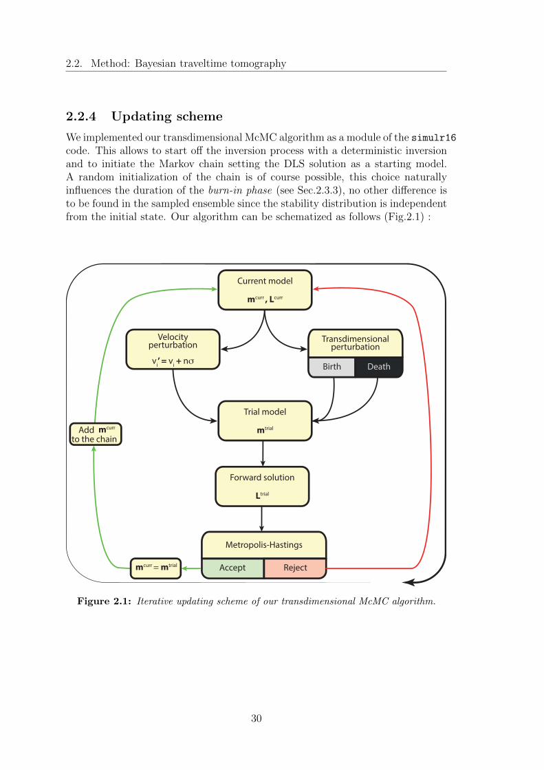
2.2. Method: Bayesian traveltime tomography
2.2.4 Updating scheme
We implemented our transdimensional McMC algorithm as a module of the simulr16code. This allows to start off the inversion process with a deterministic inversionand to initiate the Markov chain setting the DLS solution as a starting model.A random initialization of the chain is of course possible, this choice naturallyinfluences the duration of the burn-in phase (see Sec.2.3.3), no other difference isto be found in the sampled ensemble since the stability distribution is independentfrom the initial state. Our algorithm can be schematized as follows (Fig.2.1) :
Current model
mcurr , Lcurr
Velocity perturbation
vi’ = v
i + nσ
Accept Reject
Metropolis-Hastings
Birth Death
Transdimensionalperturbation
Trial model
mtrial
mcurr = mtrial
Forward solution
Ltrial
mcurr Addto the chain
Figure 2.1: Iterative updating scheme of our transdimensional McMC algorithm.
30
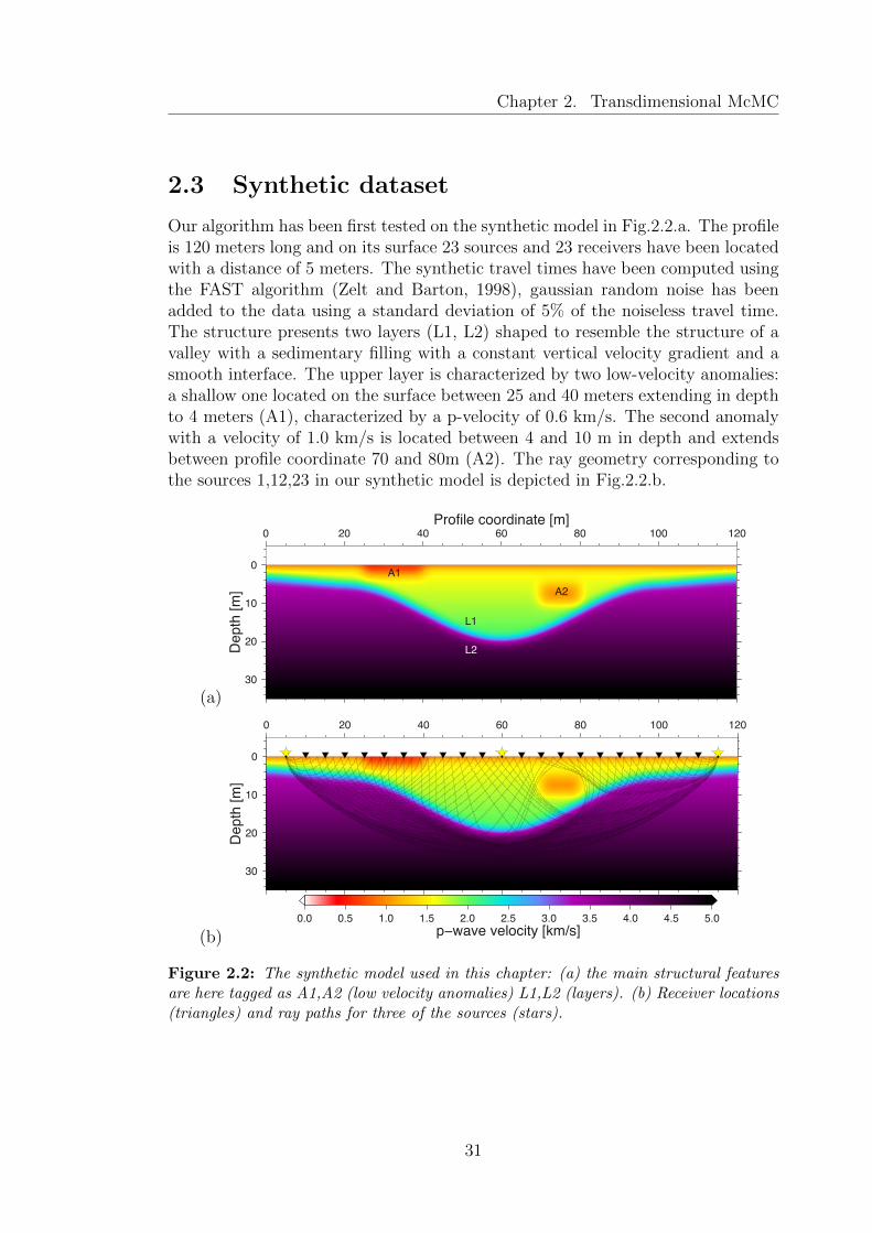
Chapter 2. Transdimensional McMC
2.3 Synthetic dataset
Our algorithm has been first tested on the synthetic model in Fig.2.2.a. The profileis 120 meters long and on its surface 23 sources and 23 receivers have been locatedwith a distance of 5 meters. The synthetic travel times have been computed usingthe FAST algorithm (Zelt and Barton, 1998), gaussian random noise has beenadded to the data using a standard deviation of 5% of the noiseless travel time.The structure presents two layers (L1, L2) shaped to resemble the structure of avalley with a sedimentary filling with a constant vertical velocity gradient and asmooth interface. The upper layer is characterized by two low-velocity anomalies:a shallow one located on the surface between 25 and 40 meters extending in depthto 4 meters (A1), characterized by a p-velocity of 0.6 km/s. The second anomalywith a velocity of 1.0 km/s is located between 4 and 10 m in depth and extendsbetween profile coordinate 70 and 80m (A2). The ray geometry corresponding tothe sources 1,12,23 in our synthetic model is depicted in Fig.2.2.b.
(a)
0
10
20
30
De
pth
[m
]
0 20 40 60 80 100 120
Profile coordinate [m]
A1
A2
L1
L2
(b)
0
10
20
30
De
pth
[m
]
0 20 40 60 80 100 120
0.0 0.5 1.0 1.5 2.0 2.5 3.0 3.5 4.0 4.5 5.0
p−wave velocity [km/s]
Figure 2.2: The synthetic model used in this chapter: (a) the main structural featuresare here tagged as A1,A2 (low velocity anomalies) L1,L2 (layers). (b) Receiver locations(triangles) and ray paths for three of the sources (stars).
31

2.3. Synthetic dataset
2.3.1 Multiple Parallel Markov Chains
High-dimensional, non-linear inverse problems can be really computer-intensive.The models that we are presenting and inverting in this paper can easily require2-4 weeks-long runtimes on a desktop computer (Intel Core i7-2600 Processor, at3.40 GHz) in order to sample a satisfying number of models. It’s therefore obvi-ous that solutions to speed up the sampling process are highly desirable. Parallelcomputing technology is nowadays easily accessible thanks to the wide diffusionof multiple-cores, multiple-CPUs architectures on almost every consumer worksta-tion. Parallelizing our algorithm seemed, hence, a straightforward solution to theneed of a speedup in the sampling process. There are two different approachesin the parallelizations of McMC algorithms: parallelizing a single Markov Chainprocess, or running multiple chains in parallel. Given the intrinsic serial nature ofMcMC simulations, the most immediate of the approaches is therefore to generatea separate Markov Chain on different CPUs/cores and then appropriately com-bine their results (Brockwell, 2006). The main advantage of this “multiple chains”approach is that almost no extra coding needs to be done. One main issue hasto be taken into account in this parallel computing environment: the burn-in. Aportion of the time spent by every chain is “wasted” producing samples that mustbe discarded, and since a burn-in period must be spent on each of the multiplechains, the final speed-up function will be less then linear (Rosenthal, 2000), asshown in Fig.2.3.
Speedup(N) =m+ bmN+ b
(2.19)
In eq.(2.19) b is the number of the burn-in models, m are the post-burn-in models,and N the number of available CPUs.
Figure 2.3: Speedup relations fora multiple chains approach showingthe theoretical linear speedup (black)in case of no burn-in (perfect paral-lelization), the curve (red) for an hy-pothetical case where the initial 10%of the models is discarded and thecurve (green) for the 0.5%-burn-inwe obtained in the inversion of theSalzach dataset (see section 2.4)
0
5
10
15
20
25
30
35
40
0 5 10 15 20 25 30 35 40
sp
ee
du
p (
N)
N - number of CPUs
perfect parallelizationburn-in 10%
burn-in 0.5%
32
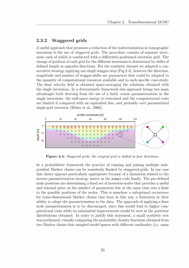
Chapter 2. Transdimensional McMC
2.3.2 Staggered grids
A useful approach that promises a reduction of the indetermination in tomographicinversions is the use of staggered grids. The procedure consists of separate inver-sions each of which is conducted with a differently-positioned inversion grid. Thechange of position of each grid for the different inversions is determined by shifts ofdefined length in opposite directions. For the synthetic dataset we adapted a con-servative strategy applying one single stagger-step (Fig.2.4), however the direction,magnitude and number of stagger-shifts are parameters that could be adapted tothe quantity of computational resources available and to each specific case-study.The final velocity field is obtained space-averaging the solutions obtained withthe single inversions. In a deterministic framework this approach brings two mainadvantages both deriving from the use of a fairly coarse parametrization in thesingle inversions: the null-space energy is restrained and the computational costsare limited if compared with an equivalent fine, and probably over parametrizedsingle-grid inversion (Bohm et al., 2000).
0
10
20de
pth
[m
]
0 20 40 60 80 100 120
profile coordinate [m]
Figure 2.4: Staggered grids: the original grid is shifted in four directions.
In a probabilistic framework the practice of running and joining multiple inde-pendent Markov chains can be seamlessly flanked by staggered-grids. In our casethis choice appears particularly appropriate because of a limitation related to theinverse parametrization strategy native in the simul code family. The pre-definednode positions are determining a fixed set of inversion-nodes that provides a usefuland rational prior on the number of parameters but at the same time sets a limitto the possible positions of the nodes. This is somehow a suboptimal occurrencefor trans-dimensional Markov chains that have in this way a limitation in theirability to adapt the parametrization to the data. The approach of applying a finernode parametrization is to be discouraged, since this would lead to higher com-putational costs while no substantial improvements would be seen in the posteriordistributions obtained. In order to justify this statement, a small synthetic testwas performed, visually comparing the probability density functions obtained fromtwo Markov chains that sampled model spaces with different cardinality (i.e. same
33

2.3. Synthetic dataset
synthetic model, with respectively a coarse and a fine parametrization). The PDFin Fig.2.5.a displays the probability distribution of velocity values at the depthswhere nodes are present, and it was obtained after ≈ 105 iterations. Figure 2.5.bdisplays the conditional distribution obtained after the same number of iterationsutilizing a 5-times finer node density in depth, thus a number of inverse parameters5 times higher. We can observe that the distribution doesn’t appear as smooth asthe one obtained with a coarse parametrization, this could be interpreted as a signof non-convergence: the chain has in fact to sample a model space with a highercardinality and needs more time to reach convergence. Letting the sampler runfor longer time we can see that eventually the conditional after ≈ 106 iterationsappears to be much smoother (Fig.2.5.c) thus the chain is likely to have reachedconvergence. The two approaches lead to distributions that at the same depthshave compatible values, on the other hand the sampler needs approximatively 10times more iterations in the fine-parametrized case resulting in suboptimal use ofcomputational resources. A staggered-grid approach seems to be therefore a betterstrategy that allows to join at the same time the need for higher spatial resolutionand for limited runtimes.
0
0 1 2 3 4 5 6
2.0
7.0
12.0
17.0
22.0
27.0
32.0
0.0
0.5
1.0
Probability
(a)
(a)
0
0 1 2 3 4 5 6
P−velocity [km/s]
0.01.02.03.04.05.06.07.08.09.010.011.012.013.014.015.016.017.018.019.020.021.022.023.024.025.026.027.028.029.030.031.032.033.034.035.0
0
0 1 2 3 4 5 6
0.01.02.03.04.05.06.07.08.09.010.011.012.013.014.015.016.017.018.019.020.021.022.023.024.025.026.027.028.029.030.031.032.033.034.035.0
Depth [m]
(b) (c)
mean model
standard deviation
Figure 2.5: Conditional probability density functions comparison: the same model isparametrized with a coarse node parametrization (a) and with a 5 times finer node spacing(b) and (c). The probability distributions are plotted at the same profile position only atdepths where a node is present. The PDF in (a) and (b) are plotted after 105 iterations,while in (c) after 106.
For the inversion of our synthetic data at every staggered-grid position multiplechains are run in parallel and then joined. Plotting the temporal evolution ofthe normalized misfit values (eq. 1.33) of the accepted models for the five chains(corresponding to the original parametrization, plus the four staggered positions)
34

Chapter 2. Transdimensional McMC
we can visually assess that all the chains sample the model space providing modelswhose data-fit is comparable, with misfit values oscillating in the range 100-140ms (Fig.2.6).
60
80
100
120
140
160
180
200
0 10000 20000 30000 40000 50000
mis
fit [m
s]
accepted models
chain 1chain 2chain 3chain 4chain 5
Figure 2.6: Temporal evolution of the normalized misfits for five instances of staggeredchains
2.3.3 Burn-in and convergence estimation
The length of the burn-in period and its determination are crucial factors in theperformance and quality of parallel Markov chain Monte Carlo algorithms. Sinceour McMC code only produces the chain of models and no statistical analysisis performed during the runtime, we could have visually analyzed the temporalevolution of the likelihood values and safely quantify the models to be discarded.
0
100
200
300
400
500
0 1000 2000 3000 4000 5000
mis
fit [m
s]
no. of models accepted
0 1000 2000 3000 4000 5000
no. of models accepted(a) (b)
Figure 2.7: Temporal evolution of normalized misfit values of the first 5000 modelssaved in two different Markov chains. (a) the chain initialized with a random model-state needs to have the first part of the models rejected (burn-in phase highlighted in thecyan box). (b) Having initialized the sampling process with the DLS solution no burn-inis necessary.
35

2.3. Synthetic dataset
As an alternative to this heuristic quantification, the choice of an appropriate start-ing point can also help to reduce or eliminate the burn-in time if the first model ischosen close to the target distribution (Fig.2.7). A convenient option we adopted isto initialize the sampling process with a model solution of a deterministic DampedLeast Squares inversion.Convergence assessment is a challenging task especially for transdimensional McMCapplications where the parametrization is constantly being modified. In this situ-ation it’s not possible to simply monitor the velocity values of some specific nodessince they are subject to “birth-death” perturbations. A good practice that holdsits validity in transdimensional application takes advantage of the CLT for Markovchains that under the reversibility condition grants asymptotic convergence to nor-mality. Operatively one could simply monitor the time evolution of the likelihood(or also misfit) distribution (Fig.2.8): once out of the burn-in phase the PDF ofthe likelihood should asymptotically stabilize.
5
Re
cu
rre
ncy [%
]
100 200 300
ALL
3
1
2
4
6
100 200 300
likelihood
ACCEPTED
100 200 300
REJECTED
Figure 2.8: Likelihood PDFs : probability distribution of the likelihood values of aMarkov chain for (cyan) all models proposed, (green) accepted models, (red) rejectedmodels.
One also could monitor variance, mean and modal value of these distributions inorder to obtain a quantitative tool to evaluate the convergence of a chain and toestablish a stopping-criterion (i.e. when to stop the sampling process). Monitor-ing the number of inversion parameters during an inversion could be a possibleconvergence-tool still supported by the CLT, however we practically noted in thisstudy that the dimensionality of the problem often tends to stabilize quickly at astable value, this could mislead to asses as convergence what is actually a pseudo-convergence (sometimes referred as multimodality). A last simpler alternative isagain a graphical analysis of the likelihood traces (Fig.2.6) which should perma-nently fluctuate around an average value.
36

Chapter 2. Transdimensional McMC
2.3.4 Inversion
The synthetic dataset has been inverted with our transdimensional McMC algo-rithm. The sampling process, initialized with the deterministic solution of a DLSinversion (Fig.2.9), was let run for ≈ 34 days utilizing staggered grids and multiplechains. Each staggered-grid inversion was produced shifting the original grid of2√2 meters along diagonal directions (2 m horizontal and vertical shifts) as illus-
trated in the scheme of Fig.2.4. For every staggered position 4 parallel chains runindependently. During a total (over the 20 total chains) of 14.19 Million iterations3 million models were accepted as member of the chains, for an average acceptancerate of ≈ 21%. The stopping-criterion adopted aimed to the collection of 3 millionmodels, value that by means of previous runs of the algorithm has been estimatedas widely sufficient to avoid pseudo-convergence and to grant the saturation of thesampled posterior distribution.
0.5 1.0 1.5 2.0 2.5 3.0 3.5 4.0 4.5 5.0
p−wave velocity [km/s]
0
10
20
30
de
pth
[m
]
0 20 40 60 80 100 120
profile coordinate [m]
3.0
1.4
0.51.4
3.0
0.5
Figure 2.9: Deterministic solution model used to initialize the Markov Chain. Isolinesof the synthetic model are reported for comparison as a red dashed curve. Inversionnodes are marked with crosses.
In order to ease the comparison with the reference synthetic model, its velocitycontour lines are reported as a red dashed curve. The surface low velocity anomaly(A1), the middle one (A2), and the bedrock shape (interface L1/L2) are visualizedwith isolines, characterized respectively by 0.5, 1.4 and 3.0 km/s p-waves velocities.
0.0 0.5 1.0
resolution
0
10
20
30
de
pth
[m
]
0 20 40 60 80 100 120
profile coordinate [m]
Figure 2.10: RDE map: Resolution Diag-onal Elements
The inverse parametrization displayedin Fig.2.9 has been determined adapt-ing the number and position of the in-verse nodes with a procedure based onthe Resolution Diagonal Elements (Fig.2.10) as described by Bleibinhaus andGebrande (2006).
37

2.3. Synthetic dataset
2.3.4.1 Posterior distributions PDF
0
10
20
30
de
pth
[m
]
0 20 40 60 80 100 120
profile coordinate [m]
Figure 2.11: Locations of the PDF verticalcross sections on the model: solid blue lines.
Probability density functions (PDFs)or posterior distributions can be re-ferred as the actual “solutions” of aninverse problem from a Bayesian per-spective. The statistical informationcontained in the PDF provide all whatis needed to infer the most importantproperties of the sampled model ensem-ble. Posterior distributions of the ve-locity field obtained with our multiple-staggered grid approach are shown in Fig.2.12 as vertical profiles at profile coordi-nates 35, 60 and 75 m in correspondence of the two low velocity anomalies (A1, A2)and at the centre of the profile. These PDFs are computed from the ensemble ofsampled models and display all the velocity values assumed by each single inverseparameter, together with the relative probability (normalized to each depth).
Figure 2.12: continues on next page
(a)
0
10
20
0 1 2 3 4 5 6 7 8
P−velocity [km s−1]
PDF at profile position 35 (m)
Mean model
Standard deviation
Deterministic solution
Synthetic model
0.0
0.5
1.0
Probability
38

Chapter 2. Transdimensional McMC
(b)
0
10
20
De
pth
[m
]
0 1 2 3 4 5 6 7 8
P−velocity [km s−1]
PDF at profile position 60 (m)
Mean model
Standard deviation
Deterministic solution
Synthetic model
0.0
0.5
1.0P
rob
ab
ility
(c)
0
10
20
De
pth
[m
]
0 1 2 3 4 5 6 7 8
P−velocity [km s−1]
PDF at profile position 75 (m)
Mean model
Standard deviation
Deterministic solution
Synthetic model
0.0
0.5
1.0
Pro
ba
bili
ty
Figure 2.12: Probability density functions (PDF): vertical cross sections at profilepositions 30, 60 and 75 m. displaying the posterior velocity distribution as wellas vertical profiles of the synthetic model, of the DLS solution, the mean posteriorand its confidence interval delimited by one standard deviation.
39
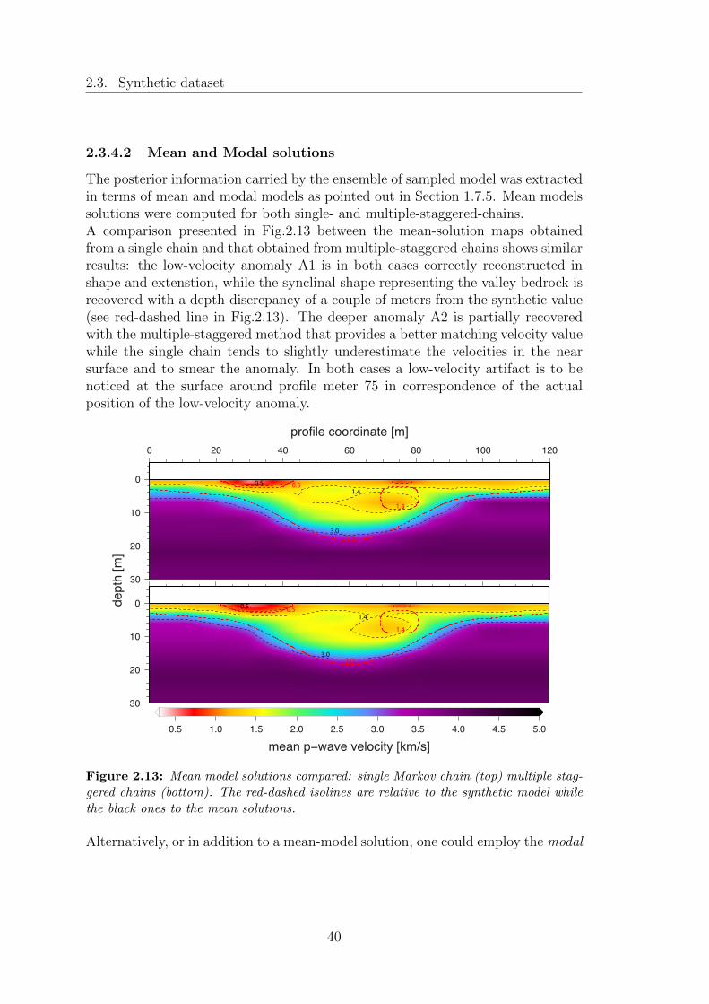
2.3. Synthetic dataset
2.3.4.2 Mean and Modal solutions
The posterior information carried by the ensemble of sampled model was extractedin terms of mean and modal models as pointed out in Section 1.7.5. Mean modelssolutions were computed for both single- and multiple-staggered-chains.A comparison presented in Fig.2.13 between the mean-solution maps obtainedfrom a single chain and that obtained from multiple-staggered chains shows similarresults: the low-velocity anomaly A1 is in both cases correctly reconstructed inshape and extenstion, while the synclinal shape representing the valley bedrock isrecovered with a depth-discrepancy of a couple of meters from the synthetic value(see red-dashed line in Fig.2.13). The deeper anomaly A2 is partially recoveredwith the multiple-staggered method that provides a better matching velocity valuewhile the single chain tends to slightly underestimate the velocities in the nearsurface and to smear the anomaly. In both cases a low-velocity artifact is to benoticed at the surface around profile meter 75 in correspondence of the actualposition of the low-velocity anomaly.
0.5 1.0 1.5 2.0 2.5 3.0 3.5 4.0 4.5 5.0
mean p−wave velocity [km/s]
0
10
20
30
3.0
1.4
0.5
1.4
3.0
0.5
0
10
20
30
de
pth
[m
]
0 20 40 60 80 100 120
profile coordinate [m]
3.0
1.4
0.5
3.0
0.5
1.4
Figure 2.13: Mean model solutions compared: single Markov chain (top) multiple stag-gered chains (bottom). The red-dashed isolines are relative to the synthetic model whilethe black ones to the mean solutions.
Alternatively, or in addition to a mean-model solution, one could employ the modal
40

Chapter 2. Transdimensional McMC
solution model obtained as the maximum of the posterior distribution. In case ofskewed or multi-modal PDFs the analysis of the modal velocity map could provideinformation useful for the interpretation. In the modal-solution in Fig.(2.14) thedeeper low-velocity anomaly appears less smeared, in addition, the high veloci-ties in the bottom part of the model are closer to the synthetic values than thecorresponding mean values.
0.5 1.0 1.5 2.0 2.5 3.0 3.5 4.0 4.5 5.0
modal p−wave velocity [km/s]
0
10
20
30
de
pth
[m
]
0 20 40 60 80 100 120
profile coordinate [m]
3.0
1.4
0.5
1.4
3.0
0.5
Figure 2.14: Modal velocity model corresponding to the multiple-staggered Markovchain.
2.3.4.3 Uncertainty map
A valuable tool in bayesian tomographic inversion is a quantitative error estima-tion. CLT and ergodic theorem once again provide the support to the computationof error maps through eq.(1.34) where the expectation is computed on h(m) thathere becomes the variance of the posterior:
Ep [h(m)] =1
M
√ M∑i=1
(mi − m)2 (2.20)
As expected well-constrained areas are located on the surface of the model, whilethe bottom part has higher uncertainty (Fig.2.15). The depth dependency of thestandard error can be also visualized on the posterior density functions (Fig.2.12).The relative standard error map (Fig.2.16) highlights the central area of the modelas that where the larger relative discrepancies with the synthetic model are to beexpected. This map is derived computing the ratio between the standard deviationand the mean model, normalized to 100.
41
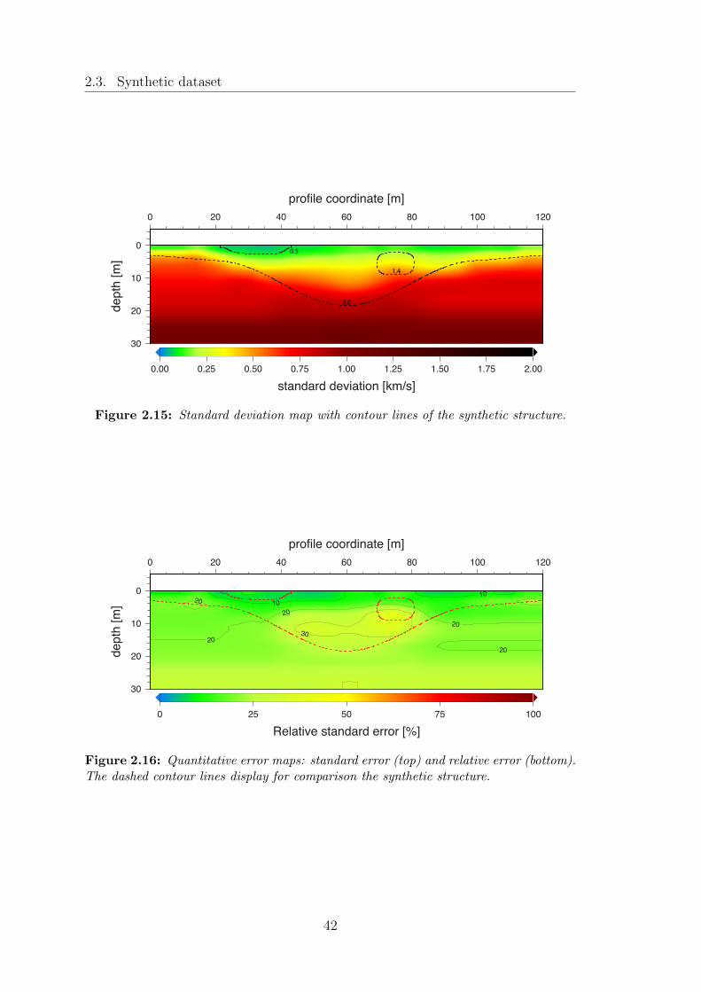
2.3. Synthetic dataset
0.00 0.25 0.50 0.75 1.00 1.25 1.50 1.75 2.00
standard deviation [km/s]
0
10
20
30
de
pth
[m
]
0 20 40 60 80 100 120
profile coordinate [m]
3.0
1.4
0.5
Figure 2.15: Standard deviation map with contour lines of the synthetic structure.
0 25 50 75 100
Relative standard error [%]
10
10
10
20
20
20
20
20
30
0
10
20
30
de
pth
[m
]
0 20 40 60 80 100 120
profile coordinate [m]
Figure 2.16: Quantitative error maps: standard error (top) and relative error (bottom).The dashed contour lines display for comparison the synthetic structure.
42

Chapter 2. Transdimensional McMC
2.4 Salzach valley
The transdimensional McMC algorithm with multiple-staggered chains was testedon a seismic dataset acquired in the year 2009 with the purpose to image theshape and structure of the Salzach Valley near Zell-am-See, Austria. A seismicline was deployed perpendicularly to the Salzach river running across the valleyand crossing the valley floor and part of the bedrock at its extremities (Fig.2.17).
12˚30' 13˚00'
47˚30'
0 10 20
Salzburg
Zell am See
Salzach
Saal
ach
SalzburgBasin
Zell BasinSalzach
0
1
2
3
km
Figure 2.17: Map of the Salzach river valley (left), the inset maps the investigationarea. Seismic profile with shot locations (circles) and receivers (red line).
The survey geometry counts eight explosive sources with an average spacing of400 m and a fixed-spread line of 10 Hz vertical-component geophones, with 10m spacing. First results from first-arrival traveltime tomography (FATT) werepublished by Bleibinhaus et al. (2010). In deep interpretation including refraction-reflection traveltime tomography (RRTT), full waveform inversion (FWI), radarand resistivity methods have been presented by Bleibinhaus and Hilberg (2012).The inverse parametrization for RRTT is formed by a set of velocity and a reflector-depth nodes. The two-steps velocity interpolation performed to obtain a smoothvelocity field starting from the coarse node-based parameterization is described inBleibinhaus and Hilberg (2012).The models of seismic velocity by Bleibinhaus and Hilberg (2012) show a quite
43
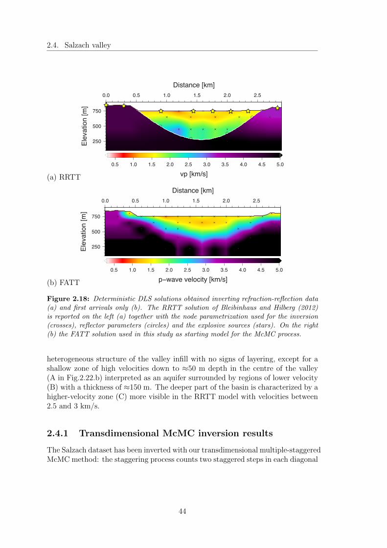
2.4. Salzach valley
(a) RRTT
0.5 1.0 1.5 2.0 2.5 3.0 3.5 4.0 4.5 5.0
vp [km/s]
250
500
750
Ele
va
tio
n [m
]
0.0 0.5 1.0 1.5 2.0 2.5
Distance [km]
(b) FATT
0.5 1.0 1.5 2.0 2.5 3.0 3.5 4.0 4.5 5.0
p−wave velocity [km/s]
1
250
500
750
Ele
va
tio
n [m
]
0.0 0.5 1.0 1.5 2.0 2.5
Distance [km]
Figure 2.18: Deterministic DLS solutions obtained inverting refraction-reflection data(a) and first arrivals only (b). The RRTT solution of Bleibinhaus and Hilberg (2012)is reported on the left (a) together with the node parametrization used for the inversion(crosses), reflector parameters (circles) and the explosive sources (stars). On the right(b) the FATT solution used in this study as starting model for the McMC process.
heterogeneous structure of the valley infill with no signs of layering, except for ashallow zone of high velocities down to ≈50 m depth in the centre of the valley(A in Fig.2.22.b) interpreted as an aquifer surrounded by regions of lower velocity(B) with a thickness of ≈150 m. The deeper part of the basin is characterized by ahigher-velocity zone (C) more visible in the RRTT model with velocities between2.5 and 3 km/s.
2.4.1 Transdimensional McMC inversion results
The Salzach dataset has been inverted with our transdimensional multiple-staggeredMcMC method: the staggering process counts two staggered steps in each diagonal
44
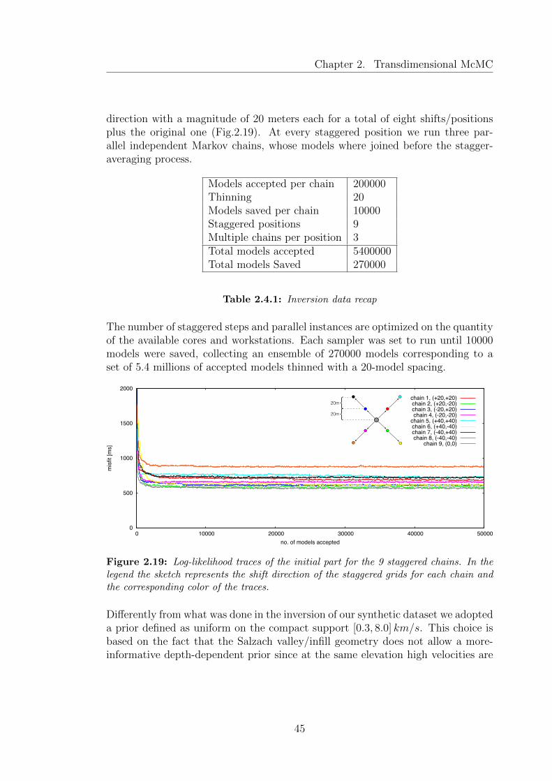
Chapter 2. Transdimensional McMC
direction with a magnitude of 20 meters each for a total of eight shifts/positionsplus the original one (Fig.2.19). At every staggered position we run three par-allel independent Markov chains, whose models where joined before the stagger-averaging process.
Models accepted per chain 200000Thinning 20Models saved per chain 10000Staggered positions 9Multiple chains per position 3Total models accepted 5400000Total models Saved 270000
Table 2.4.1: Inversion data recap
The number of staggered steps and parallel instances are optimized on the quantityof the available cores and workstations. Each sampler was set to run until 10000models were saved, collecting an ensemble of 270000 models corresponding to aset of 5.4 millions of accepted models thinned with a 20-model spacing.
0
500
1000
1500
2000
0 10000 20000 30000 40000 50000
mis
fit [m
s]
no. of models accepted
chain 1, (+20,+20)chain 2, (+20,-20)chain 3, (-20,+20)chain 4, (-20,-20)
chain 5, (+40,+40)chain 6, (+40,-40)chain 7, (-40,+40)chain 8, (-40,-40)
chain 9, (0,0)
{{20m
20m
Figure 2.19: Log-likelihood traces of the initial part for the 9 staggered chains. In thelegend the sketch represents the shift direction of the staggered grids for each chain andthe corresponding color of the traces.
Differently from what was done in the inversion of our synthetic dataset we adopteda prior defined as uniform on the compact support [0.3, 8.0] km/s. This choice isbased on the fact that the Salzach valley/infill geometry does not allow a more-informative depth-dependent prior since at the same elevation high velocities are
45

2.4. Salzach valley
present (bedrock) together with lower ones (infill). The prior on the number ofnodes was set as uniform in [1, 59]. The standard deviation of the proposal distri-bution (σ in eq. 2.6 and 2.7) is scaled at every node to a value that correspondsto 5% of the velocity obtained in the same position from the deterministic solu-tion (2.18.b) used to initialize the sampling process. In this way the characteristicperturbation size is smaller for nodes that are expected to have lower velocity andbigger for nodes in faster areas of the model. Such a choice is meant to grant op-timized mixing for all nodes, however other values for the proposal width σ wouldmainly influence the performances of the sampler, in terms of mixing properties andacceptance rate, thus the resulting posterior distributions are not supposed to beinfluenced by our choice. We discarded the first 1000 models of every chain (0.5%of all the accepted models), allowing the samplers to settle and oscillate arounda stable number of inversion nodes, as well around a stable likelihood value. Thefact that the chain related to the original grid (the grey trace in Fig.2.19) appearsto sample better models (with lower misfits) should not turn out surprising: thatparametrization is in fact the result of an optimization process aimed to identifyan optimal parametrization, some of the grid shifts in the staggering process mightindeed lead to less optimal parametrizations. This might result indeed in sampledmodels characterized by an average lower level of data fit. It might in other caseslead as well to the opposite situation.
Figure 2.20: continues on next page
(a)
300
400
500
600
700
Ele
va
tio
n [m
]
0 1 2 3 4 5 6 7 8
P−velocity [km s−1]
PDF at profile position 1.0 (km)
Mean model
Standard deviation
Deterministic solution
Modal model
0.0
0.5
1.0
Pro
ba
bili
ty
46
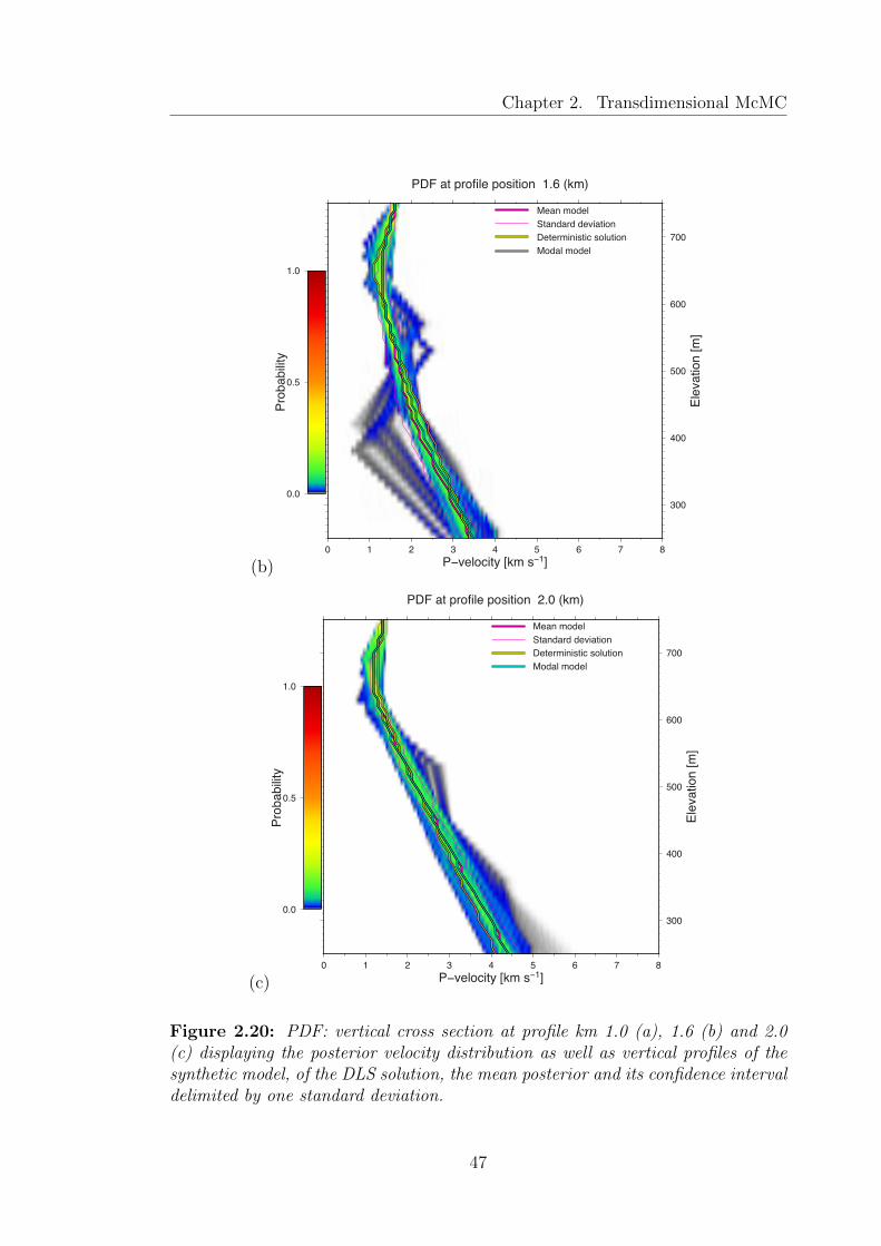
Chapter 2. Transdimensional McMC
(b)
300
400
500
600
700
Ele
va
tio
n [m
]
0 1 2 3 4 5 6 7 8
P−velocity [km s−1]
PDF at profile position 1.6 (km)
Mean model
Standard deviation
Deterministic solution
Modal model
0.0
0.5
1.0P
rob
ab
ility
(c)
300
400
500
600
700
Ele
va
tio
n [m
]
0 1 2 3 4 5 6 7 8
P−velocity [km s−1]
PDF at profile position 2.0 (km)
Mean model
Standard deviation
Deterministic solution
Modal model
0.0
0.5
1.0
Pro
ba
bili
ty
Figure 2.20: PDF: vertical cross section at profile km 1.0 (a), 1.6 (b) and 2.0(c) displaying the posterior velocity distribution as well as vertical profiles of thesynthetic model, of the DLS solution, the mean posterior and its confidence intervaldelimited by one standard deviation.
47

2.4. Salzach valley
2.4.1.1 Posterior distributions
The a posteriori distributions of the sampled velocities are displayed as cross sec-tions at profile coordinates 1.0 (Fig.2.20.a), 1.6 (Fig.2.20.b) and 2.0 km (Fig.2.20.c),together with the correspondent vertical velocity profiles extracted from the de-terministic solution model, the modal and the mean solution with it’s confidenceinterval defined with plus/minus one standard deviation. In order to ease the com-parison between different methods, the FATT solution of Bleibinhaus and Hilberg(2012), computed on a static grid, is from here on substituted with a staggeredFATT solution obtained with the same method, but applying in addition also thestaggered grid approach described in the previous paragraph. This allows a faircomparison between models obtained from deterministic and probabilistic inver-sion methods. The PDFs at profile coordinates 1.0 (Fig.2.20.a) and 1.6 (Fig.2.20.b)show a multimodal behavior, with sets of low-likely models that deviate from themain, most-likely portion of the distribution. This effect is ascribed to the use ofstaggered grids: some of the staggered chains are spending some time samplinga less relevant part of the model space in the attempt to fit the data, given thestaggered parametrization. Such an outcome is however not to be regarded as neg-ative for the sampling process. The extremely low probability that characterizesthis portion of sampled models leads them in fact to have a negligible influence onthe inversion results.
Figure 2.21: Posterior distribu-tion on the number of inverse pa-rameters for the ensemble. Themodal value corresponds to 33nodes.
0
5
10
15
20
25
30
Recurr
ency [%
]
20 30 40 50
no.nodes
The PDF of the number of nodes extracted from the models ensemble (Fig.2.21)points out that the sampling process clearly favored models parametrized with 33nodes, a slight multimodal behavior is however to be noted with two minor peaksat 37 and 39.
48

Chapter 2. Transdimensional McMC
2.4.1.2 Transdimensional inversion results
As done for our synthetic case-study, we extracted as a representative model so-lution the mean of the sampled ensemble. This transdimensional McMC stag-gered mean model (Fig.2.22.a) shows an overall good level of agreement with thesolutions obtained through deterministic approaches: Full Waveform Inversion(Fig.2.22.b), Reflection-Refraction (Fig.2.22.c) and First Arrival Traveltime To-mography (Fig.2.22.d).The shape of the Salzach valley bedrock we obtained yields some structural detailsthat find correspondence in the FWI solution (green arrows in Fig.2.22.a and b)while they could not be recovered by the RRTT (whose parametrization of thereflecting interface intrinsically removes smaller details in the structure in favorof a regular structure) and FATT solutions. The interface between valley infilland bedrock, identified considering the 3.0 km/s isoline, shows a sharper velocitycontrast in the McMC mean model compared to the FATT solution, where thesame boundary appears more blurred.The low velocity area (B) and an aquifer (A) are clearly outlined in our bayesianmean model and appear to generally confirm the solutions obtained with all theother methods. A higher level of similitude is however noticeable between the FWIand our solution, which are able to provide a level of complexity in the shape of thelow velocity area not reached by RRTT and FATT. A minor zone with velocitieslower than 1.5 km/s is present at the surface of the McMC solution between profilecoordinates 2.2 and 2.5 km, corresponding to the right extremity of the area B asproposed by the FWI solution (blue arrow in Fig.2.22.a and b). Thickness andhorizontal extension of the aquifer as recovered by our bayesian sampling processare compatible with the values proposed with all the other methods exceptionmade for the FATT staggered solution that proposes slightly higher velocities inthe near surface between km 2.0 and 2.5.The 3.0 km/s isoline that could be considered as representing the boundary be-tween valley infill and bedrock shows in the McMC solution a sub-elliptical featurethat finds a mild correspondence in the FWI solution in a lower velocity area (redarrows in Fig.2.22.a and b).The shape of the high velocity area highlighted with the letter (C) in the RRTTsolution, seems to be qualitatively confirmed by all the other methods, howeverthe estimated value of the velocity appears to be slightly lower for McMC, FWIand FATT model solutions, with values around 2.0 Km/s.
49

2.4. Salzach valley
250
500
750
0.0 0.5 1.0 1.5 2.0 2.5
Distance [km]
RRTT
FATT
0.5 1.0 1.5 2.0 2.5 3.0 3.5 4.0 4.5 5.0
p−wave velocity [km/s]
250
500
750
Ele
va
tio
n [m
]
250
500
750
1.5
2.5
3.0
AB
McMC
3.0
1.5
2.5
A
C
1.5B
A
B
2.5
3.0
250
500
750
1.52.5
AB
3.0
FWI
(a)
(b)
(c)
(d)
Figure 2.22: Solution models compared: transdimensional McMC mean model (a), de-terministic Full Waveform Inversion (b), deterministic Reflection-Refraction (c), deter-ministic first arrivals staggered (d). The arrows refer to features recovered with differentmethods, discussed in the text.
50

Chapter 2. Transdimensional McMC
2.4.1.3 Error maps
The quantitative uncertainty estimate of the solution made possible by the bayesianapproach is expressed in Fig.2.23 in terms of a standard deviation map togetherwith a relative error map.
(a)
0.00 0.25 0.50 0.75 1.00 1.25 1.50 1.75 2.00
standard deviation [km/s]
250
500
750
Ele
va
tio
n [m
]
0.0 0.5 1.0 1.5 2.0 2.5
Distance [km]
0.1
0.5
0.5
(b)
0 25 50 75 100
Relative standard error [%]
250
500
750
Ele
va
tio
n [m
]
10 10 10
515
15
15
5
Figure 2.23: Standard deviation (a) and relative error (b) maps.
The uppermost part of the valley infill is characterized by uncertainties smallerthan 0.1 km/s, while in depth the standard error doesn’t exceed 0.5 km/s, valuethat could be considered as limit between infill and bedrock. The relative errormap suggests that the horizontal anomaly located on the right side of the modelat elevations between 500 and 600 m is likely to be an artifact. However, aswe already pointed out in the previous paragraph, there is a good correspondencewith the FWI solutions from Bleibinhaus and Hilberg (2012) where a discontinuityseems to characterize the bedrock at about 600 m and 2.5 km in profile direction.The area of higher uncertainty is located between km 1.0 and 1.4 on the deeperpart of the model, here uncertainties up to almost 1 km/s are to be expected.The discontinuous values of estimated uncertainty in the bottom portion of themodel (below 250 m.) raise a question on the validity of these estimates. At thesame depth, in a portion of model identified as part of the bedrock, a relatively
51

2.4. Salzach valley
wide range of uncertainties, spanning from ca. 0.20 to 1.0 km/s, appears odd. Afurther tool can help in this case to clarify the situation: a map displaying howoften nodes located in a defined area have been treated as inverse parameters orwere removed by the transdimensional sampling algorithm (Fig.2.24).
0 50 100
node recurrence [%]
250
500
750
Ele
va
tio
n [m
]
0.0 0.5 1.0 1.5 2.0 2.5
Distance [km]
Figure 2.24: Node recurrence map: the positions of possible inversion nodes (crosses)are displayed together with the relative frequency of each node being considered as aninverse parameter. Nodes that were more often set as inversion parameters have colorstending towards green, conversely less-often inverted nodes display colors towards red.
Considering the bottom portion of the model, an alternating pattern is noticed, incorrespondence to the aforementioned discontinuous values of uncertainty. Such apattern points out that some node-configurations were more often preferred duringthe sampling process. This could be interpreted as an outcome of the naturalparsimony property: a high parameter density is not needed at the bottom of themodel and therefore models with a coarse node-distance are selected with higherfrequency. Back to the issue of uncertainty estimation for the bottommost portionof the model: joining the information content of standard deviation (Fig.2.23.a)and node recurrency map (Fig.2.24) we suggest that an expected value for thestandard deviation is to be computed as an average of the values characterizingthe bottom nodes, corresponding to ≈ 0.5 km/s.
Proceeding with the uncertainty analysis, the low-velocity sub-elliptical structuremarked with a red arrow in Fig.2.22.a) is likely to be an artifact, as suggestedby the relative error map which proposes values of the relative error higher than15%. The structure could correspond to a ripple in the infill/bedrock interface asproposed by the FWI solution.
Another area where the relative error reaches values of 15% involves the lowerboundary of the low-velocity area (B) between km 1.7 and 1.8, with uncertaintiesin the order of 0.25 km/s expected to affect that portion of the model.
52

Chapter 2. Transdimensional McMC
2.5 Conclusions
We presented an algorithm that allows for the inversion of first arrival traveltimestomography data within a Bayesian framework. The process can be classified asa transdimensional Markov chain Monte Carlo, based on the Metropolis-Hastingsalgorithm. We adopted in addition a parallel-staggered grid approach that makesuse of parallel-independent McMC processes and staggered grids in order to opti-mize the performances of the inversion.The number and position of the inversion parameters is constantly changing duringthe sampling process thus is treated as an unknown of the inversion process. Theamount and distribution of information in the data drives the choice of number andspatial location of the inverse nodes, relieving the operator from the need to choseand optimize a nor parametrization, neither smoothing or damping parameters.The solution models obtained appear naturally smooth as a result of the spatialaveraging process over the sampled ensemble.The practice of running parallel-independent sampling processes is proved to bevery effective in the framework offered by the simulr16 code. The extremelyshort burn-in phases we observed leads in fact to a speedup that yields an almostlinear dependence with the number of parallel processes involved in the sampling.Making use of multiple instances of our McMC code reduces thus the run timeneeded to collect a satisfying number of models of a factor proportional to thecores/CPUs involved.A staggered grid approach was adopted, as a compensation for the relatively coarsespatial distribution of the inversion nodes that characterizes the simulr16 code.Staggered coarse grids allow to restrain the cardinality of the model space, thus re-sult in shorter runtime needed to reach convergence compared to the correspondingsingle fine-grid alternative. Furthermore models obtained through a staggered-gridapproach proved to reconstruct finer structural details without increasing the un-certainty of the solution.Our code was first tested on a synthetic dataset, and then utilized to invert fielddata from the Salzach Valley (Austria) comparing our McMC solution with someresults obtained by Bleibinhaus and Hilberg (2012) from the same data. Theresults obtained show a general agreement with the solutions proposed in thepaper of Bleibinhaus and a particularly good match is observed with the FullWave Inversion model even if our method makes use of first arrivals data only.The inversion with our transdimensional McMC code offers of possibility of aquantitative uncertainty analysis by means of standard deviation and relative errormaps. A useful tool for the interpretation of the uncertainty maps is provided bythe node recurrence map.
53

2.5. Conclusions
54

Chapter 3
Resolution Matrix for aMultivariate updating scheme
3.1 Introduction
One of the most important issues of interpreting seismic tomography models isthe need to provide a quantification of their uncertainty. Bayesian approach toinverse problems offers a rigorous way to quantitatively estimate this uncertaintyat the price of a higher computation time. Optimizing bayesian algorithms istherefore a key problem. In this chapter we present a multivariate model-updatingscheme which makes use of the constraints provided by the Model ResolutionMatrix, aiming to a more efficient sampling of the model space. The ResolutionMatrix relates the true model to the estimate, its off-diagonal values provide a setof trade-off relations between model parameters used in our algorithm to obtainoptimized model updates. The bayesian algorithm we implemented and describedin the previous chapter belongs to an important class of Markov Chain MonteCarlo methods called Random Walk Markov Chains. The trajectory of “steps”between neighboring states is a random walk and can be described with a graphin the model space. Such sampling schemes based on the Metropolis-Hastingsalgorithm require an accurate choice of proposal distributions: defining a goodproposal distribution means choosing which size and kind of random steps is moreconvenient to efficiently move between neighboring model-states. As Metropoliset al. (1953) stated in one of the first papers that employed McMC sampling: “themaximum displacement must be chosen with some care; is too large most moveswill be forbidden, and if too small, the configuration will not change enough. Ineither case it will take longer to come to equilibrium.”. Anyway not only theperturbation size is key to an optimized algorithm, also the way one tries to movebetween models is of fundamental importance.
55

3.1. Introduction
3.1.1 Optimization of Metropolis-Hastings McMC
In the first chapter of this work we focused on the formal basis that justify theimportance of reversible, ergodic Markov chains. Ergodicity is, in a broad sense,a property of stochastic processes for which the time average over a sub-sequenceof events corresponds to the global ensemble average. For Markov chains ergod-icity guarantees the existence and unicity of a stationary distribution. ReversibleMarkov chains are satisfying the detailed-balance condition, which grants the exis-tence of a stationary distribution. The behavior of reversible chains is independentfrom the time-direction of their evolution, they hold the same properties backwardsof forwards in time.
The importance of these properties combined is that, for those who are seekingto implement, modify or, like us, optimize an updating scheme, it is fundamentalto keep in mind that all the non-trivial known methods to construct updatingmechanisms able to preserve a given equilibrium distribution, are special casesof the Metropolis-Hastings (M-H) algorithm that hold the reversibility condition(C.Geyer on Brooks et al. (2011)).
Furthermore since reversibility and ergodicity allow the applicability of the Markovchain central limit theorem (see eq.1.14) and asymptotic variance estimation, thepreservation of such properties grants the possibility to estimate the expectationsof some quantity related to the sampled ensembles (provided that the sampleris given enough time to reach convergence, i.e. to sample a sufficient number ofmodels).
Optimal performances of McMC samplers based on the M-H algorithm are directlyconnected with the optimization of the M-H ratio (eq.1.27). The main points toconsider are therefore:
• Likelihood: an appropriate function has to be utilized to quantify the abilityof a model to fit observed data, this includes a proper estimate of the datanoise. This work will not focus particularly on this aspect, however someinteresting treatise and examples can be found in Pearse et al. (2009) andBodin et al. (2012).
• Prior: a priori knowledge should be included in the algorithm with a prob-abilistic formulation, limiting where possible the model space to be sampled.Some consideration will be given in section 3.2.3.
• Proposal: how to efficiently and correctly propose new models. Efficiencyis directly connected with the size of the “steps” between models while cor-rectness relates to the updating scheme used, i.e. to how models are modifiedto produce new candidates.
56

Chapter 3. Resolution Matrix for a Multivariate updating scheme
In this chapter we will focus on this third point and propose a method that, througha multivariate updating mechanism, aims to increase the sampling efficiency whilepreserving fundamental properties that characterize Metropolis-Hastings updatingschemes.
3.1.2 Comparing the efficiency of Markov Chains
Our purpose is, as said, to propose an optimized transition kernel (proposal distri-bution) that leads to a better McMC algorithm, therefore we first need to definewhat “better Markov chain” means and to point out some criteria that could beused to compare the efficiency of Markov Chains. Let’s then lay down, followingthe lead of J. Rosenthal in Brooks et al. (2011, Chap.4), some rules to comparetwo chains {Xi} with transition kernels P1(x,A) and P2(x,A) both with the samestationary distribution π: convergence speed, variance and mixing properties.
Convergence speed: Using the measure of variational distance introduced witheq.(1.8), the chain with kernel P1 shows a faster convergence than P2 if:
supA |P n1 (x,A)− π(A)| ≤ supA |P n
2 (x,A)− π(A)| ∀n, x (3.1)
In other words, if at the nth iterate of the transition kernel (eq.1.4), the conditionaldistribution of the chain P1 is closer to the equilibrium distribution than the chainP2, this means that the chain P1 has been converging faster than P2.
Variance: As a second criterion we consider some appropriate functional g(Xi)of the chain and use it to compute a variance in the form:
V (g) = V ar
(1
n
N∑i=1
g(Xi)
)(3.2)
then the chain following the transition kernel P1 is more efficient if it has a smallervariance than the chain following P2. This definition could however be dependenton the choice of the functional g and on the initial distribution X0. Usual practiceis to compare chains in stationarity, therefore after a long runtime. Anyway fora sufficient number of iterates of a transition kernel, the memory of the initialdistribution should be lost.
Mixing: The third and last criterion is probably the most intuitive since it ba-sically states that a chain is better if it allows a faster sampling of the modelspace.
57
3.1. Introduction
E∥∆X∥ = E[(Xn −Xn−1)
2]
(3.3)
Where the function E∥∆X∥ measures the distance from one member of a chain Xn
to the previous oneXn−1, this can be accomplished for example with any functionallike 1
N
∑Ni=1(Xi−Xi−1)
2 (N is the number of states in the chain considered for themeasure). If the estimate of the expectation, is bigger for P1 than for P2 we willsay that the first chain shows a faster mixing. The value of eq.(3.3) is computedon all the steps of the sampler thus rejected steps will give a null contribution andsmall accepted ones will not help that much either and will also push towards anoverall slowly-sampling chain. These different definitions can be to some extentmerged into the single relaxed statement that a better Markov chain samples themodel space more efficiently if it reaches the equilibrium distribution faster, itdoesn’t extensively sample low-likelihood areas and it proceeds in the samplingwith steps that at the same time are not so big to be often rejected nor so smallto be irrelevant.Further diagnostic tools we will utilize include a qualitative analysis of the traceplots of single model parameters. The time evolution of the sampled values forsome selected nodes is plotted and analyzed to graphically highlight the mixingbehavior of different transition kernels, i.e. how big and how frequent are the stepsbetween parameter values. If with eq.(3.3) the whole model is taken into account,with a measure of distance that involves all the parameters, a more simplistic anal-ysis can be performed observing single parameters. Basic principles and examplesof trace plots analysis can be found in Brooks et al. (2011, pp.95-98).Another aspect of analyzing mixing properties is to understand how the pertur-bations applied to a model reflect in the likelihood of a trial model. A proposedstep between model-states could be significant in terms of distance (chosen anappropriate metric for eq.3.3), but could at the same time lead to a proposedstate whose likelihood is close to that of the previous state and therefore morelikely to be accepted. To understand this behavior we will take into account theprobability distributions of likelihood differences (LD) between current and trialmodels LD = LC − LT to visualize the size of the “likelihood-steps” togetherwith their probability. Proposed model whose LD is close to zero are more likelyto be accepted, therefore comparing Markov chains, transition kernels leading toLD-distributions more peaked around zero will be considered more efficient.
58
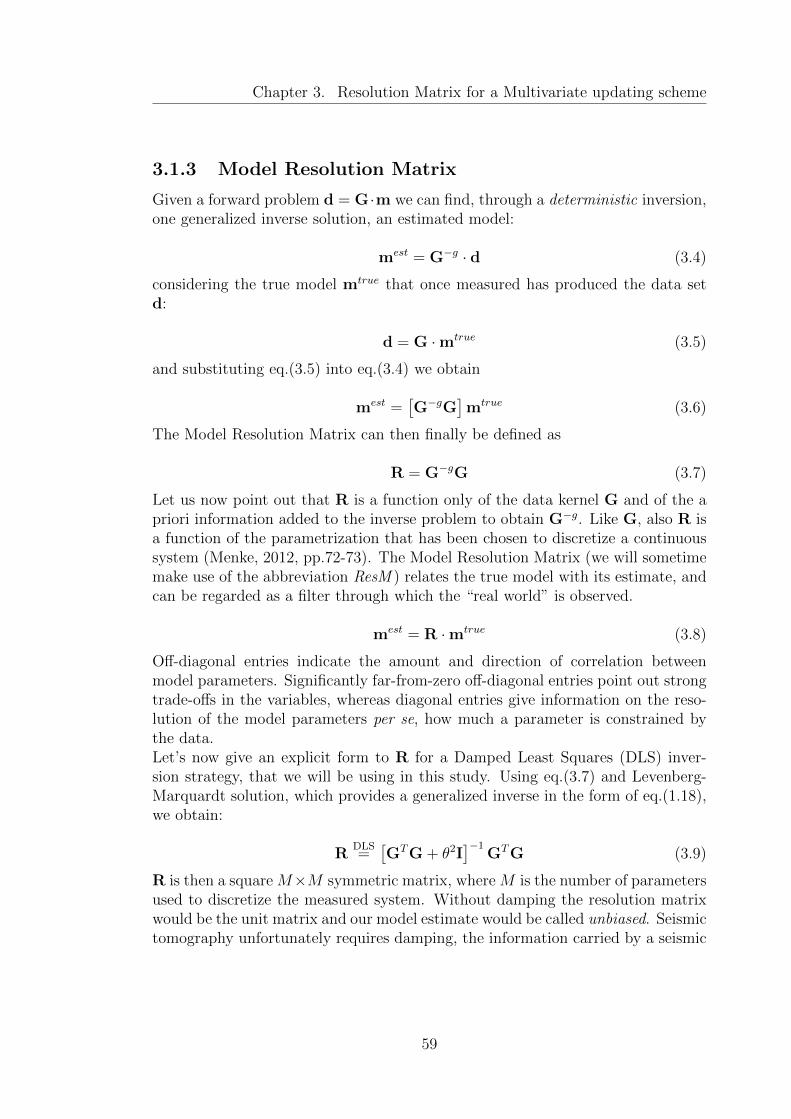
Chapter 3. Resolution Matrix for a Multivariate updating scheme
3.1.3 Model Resolution Matrix
Given a forward problem d = G ·m we can find, through a deterministic inversion,one generalized inverse solution, an estimated model:
mest = G−g · d (3.4)
considering the true model mtrue that once measured has produced the data setd:
d = G ·mtrue (3.5)
and substituting eq.(3.5) into eq.(3.4) we obtain
mest =[G−gG
]mtrue (3.6)
The Model Resolution Matrix can then finally be defined as
R = G−gG (3.7)
Let us now point out that R is a function only of the data kernel G and of the apriori information added to the inverse problem to obtain G−g. Like G, also R isa function of the parametrization that has been chosen to discretize a continuoussystem (Menke, 2012, pp.72-73). The Model Resolution Matrix (we will sometimemake use of the abbreviation ResM ) relates the true model with its estimate, andcan be regarded as a filter through which the “real world” is observed.
mest = R ·mtrue (3.8)
Off-diagonal entries indicate the amount and direction of correlation betweenmodel parameters. Significantly far-from-zero off-diagonal entries point out strongtrade-offs in the variables, whereas diagonal entries give information on the reso-lution of the model parameters per se, how much a parameter is constrained bythe data.Let’s now give an explicit form to R for a Damped Least Squares (DLS) inver-sion strategy, that we will be using in this study. Using eq.(3.7) and Levenberg-Marquardt solution, which provides a generalized inverse in the form of eq.(1.18),we obtain:
RDLS=[GTG+ θ2I
]−1GTG (3.9)
R is then a squareM×M symmetric matrix, whereM is the number of parametersused to discretize the measured system. Without damping the resolution matrixwould be the unit matrix and our model estimate would be called unbiased. Seismictomography unfortunately requires damping, the information carried by a seismic
59

3.1. Introduction
ray is an integral over the whole ray path, influenced by several parameters. Thebetter a parameter is resolved, the moreR will tend to the unity matrix. Explicitlywriting the ith row of eq.(3.8) we have:
mesti =
M∑j=1
Rij ·mtruej (3.10)
where we can see that the estimate of each model parameter is a weighted averageof the whole true model. The ith row of R provides the weighting factors for the ith
parameter. The trace of R is sometimes regarded as an estimation of the degreesof freedom in the model, which is considered as the number of parameters thatthe dataset can resolve. For an ideally unbiased model, when R = 1, the numberof degrees of freedom would equal the number of model parameters M , but foralmost every geophysical underdetermined problem the off diagonal elements ofthe resolution matrix will be non-zero and
∑Mj=1Rij < 1 (Nolet, 2008, p.278).
Such situation, as for the example pictured in Fig.3.1, indicates the intrinsic limitsof the inversion process and the inability to separate the effects and influence onthe ith parameter of all the others.
Figure 3.1: A graphical representation of equation 3.8 relating a synthetic seismicvelocity model (right) to one possible DLS-solution (left) through the model resolutionmatrix (middle). The ith row of R shows how a perturbation of the true synthetic modelwill be mapped into the inverse parameters of mest. Well resolved inverse parametershave higher diagonal-element values (Rii ≈ 1, darker colors), poorly resolved parameterswith almost zero resolution will tend to white.
In this study we will make use of the information carried by the resolution matrixR. This information reflects the uncertainty connected to the nature of the forwardproblem itself: how density and distribution of the data are expected to be resolvedgiven a certain parametrization. Trade-off relations between model parameterswill be exploited in the next section in order to implement a more efficient McMCupdating scheme for a Markov chain Monte Carlo algorithm.
60
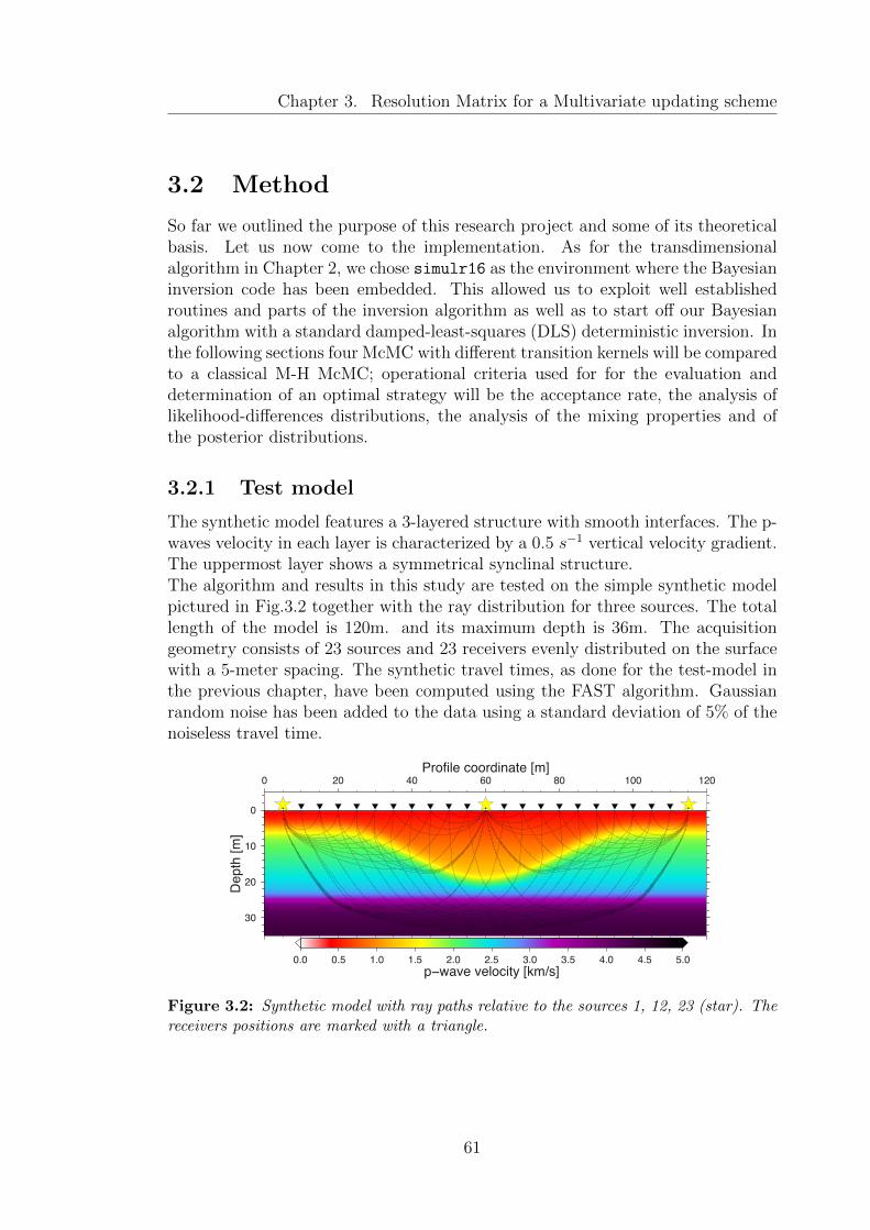
Chapter 3. Resolution Matrix for a Multivariate updating scheme
3.2 Method
So far we outlined the purpose of this research project and some of its theoreticalbasis. Let us now come to the implementation. As for the transdimensionalalgorithm in Chapter 2, we chose simulr16 as the environment where the Bayesianinversion code has been embedded. This allowed us to exploit well establishedroutines and parts of the inversion algorithm as well as to start off our Bayesianalgorithm with a standard damped-least-squares (DLS) deterministic inversion. Inthe following sections four McMC with different transition kernels will be comparedto a classical M-H McMC; operational criteria used for for the evaluation anddetermination of an optimal strategy will be the acceptance rate, the analysis oflikelihood-differences distributions, the analysis of the mixing properties and ofthe posterior distributions.
3.2.1 Test model
The synthetic model features a 3-layered structure with smooth interfaces. The p-waves velocity in each layer is characterized by a 0.5 s−1 vertical velocity gradient.The uppermost layer shows a symmetrical synclinal structure.The algorithm and results in this study are tested on the simple synthetic modelpictured in Fig.3.2 together with the ray distribution for three sources. The totallength of the model is 120m. and its maximum depth is 36m. The acquisitiongeometry consists of 23 sources and 23 receivers evenly distributed on the surfacewith a 5-meter spacing. The synthetic travel times, as done for the test-model inthe previous chapter, have been computed using the FAST algorithm. Gaussianrandom noise has been added to the data using a standard deviation of 5% of thenoiseless travel time.
0
10
20
30
De
pth
[m
]
0 20 40 60 80 100 120Profile coordinate [m]
0.0 0.5 1.0 1.5 2.0 2.5 3.0 3.5 4.0 4.5 5.0
p−wave velocity [km/s]
Figure 3.2: Synthetic model with ray paths relative to the sources 1, 12, 23 (star). Thereceivers positions are marked with a triangle.
61

3.2. Method
3.2.2 Deterministic inversion
A damping test is performed and the parametrization adapted choosing an opti-mal node distribution with the same general workflow that has been described inBleibinhaus and Hilberg (2012). The solution obtained is then used as the startingmodel in our McMC. This particular choice of the deterministic solution as initialstate for the Markov chain as well as the decision to use an adapted parametriza-tion are of course arbitrary choices, but we can nonetheless motivate them withsome considerations.
First of all on the use of the deterministic solution as starting model for theMarkov chain: any valid starting point we could choose is as good as any otherpoint in the model space that might have been randomly picked out of the priordistribution. Any velocity model is allowed to be chosen as the first memberof a Markov chain, so why not starting from a point of the model space thathas a high probability of being close, if not inside, the equilibrium distributionBrooks et al. (2011). Since of course such a distribution is unknown before thesampling process we can assume that a solution of a DLS inversion will likelyhave the desired property of vicinity to the equilibrium distribution. This willhave the positive effect of shortening the burn-in phase of the Markov chain atthe negligible price of a deterministic inversion: starting the chain in a state closeto the equilibrium saves us the time that would have otherwise been spent bythe sampler accepting many low-likelihood models in order to approach the tailof the stability distribution. A further reason for us to commence the samplingfrom the DLS solution will be made clear in the following sections and it will beshown to be a fundamental requirement for our inversion process. A second pointthat deserves consideration is the use of an adapted parametrization: the spatialdistribution and number of model parameters used in the DLS inversion leadingto the initial model is optimized, and corresponds to the inverse parametrizationused for the Bayesian inversion. As the aim of the study exposed in this chapteris to probe the feasibility, the effects, and eventually the benefits of a Resolution-Matrix-based transition kernel, we preferred not to employ a transdimensionalapproach, in order to simplify the problem and to better isolate the influences ofthe ResM only. For this reason an optimized parametrization offers some benefits.A lower number of parameters is needed, with a consequent minor computationalload and faster execution of tests.
In addition to the reasons provided in the beginning of this section, the syntheticdataset has been inverted also in order to compare the results of our algorithmto a classical damped least squares inversion. The inversion process is startedwith a dense rectilinear node grid, the least resolved nodes are removed fromthe parametrization and the process (inversion-adaptation) is repeated until asatisfying compromise is reached between grid density and resolution.
62
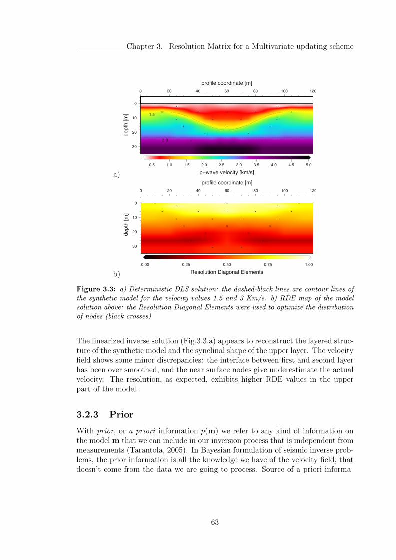
Chapter 3. Resolution Matrix for a Multivariate updating scheme
a)
0.5 1.0 1.5 2.0 2.5 3.0 3.5 4.0 4.5 5.0
p−wave velocity [km/s]
0
10
20
30
de
pth
[m
]
0 20 40 60 80 100 120
profile coordinate [m]
1.5
3.0
b)
0.00 0.25 0.50 0.75 1.00
Resolution Diagonal Elements
0
10
20
30
de
pth
[m
]
0 20 40 60 80 100 120
profile coordinate [m]
Figure 3.3: a) Deterministic DLS solution: the dashed-black lines are contour lines ofthe synthetic model for the velocity values 1.5 and 3 Km/s. b) RDE map of the modelsolution above: the Resolution Diagonal Elements were used to optimize the distributionof nodes (black crosses)
The linearized inverse solution (Fig.3.3.a) appears to reconstruct the layered struc-ture of the synthetic model and the synclinal shape of the upper layer. The velocityfield shows some minor discrepancies: the interface between first and second layerhas been over smoothed, and the near surface nodes give underestimate the actualvelocity. The resolution, as expected, exhibits higher RDE values in the upperpart of the model.
3.2.3 Prior
With prior, or a priori information p(m) we refer to any kind of information onthe model m that we can include in our inversion process that is independent frommeasurements (Tarantola, 2005). In Bayesian formulation of seismic inverse prob-lems, the prior information is all the knowledge we have of the velocity field, thatdoesn’t come from the data we are going to process. Source of a priori informa-
63

3.2. Method
tion could be previous studies, physical knowledge, or simply a reasonable rangeto which we want our velocity field to be limited. In this work a low-informativeprior (Gelman, 2006) was used to limit the p-waves velocity to a reasonable depth-dependent range. Operatively prior-velocity intervals were defined both on thesurface and on the bottom of our model, to obtain the prior at each depth throughlinear interpolation as in Fig.3.4.
Figure 3.4: Prior information: velocityranges are defined both on the surface andon the bottom of the model to obtain theprior at each depth through linear inter-polation.
0
10
20
30
De
pth
[m
]
0 1 2 3 4 5 6 7 8 9 10
P−velocity [km s−1]
Velocity prior definition
V min
TO
P
V max
TOP
V min
BO
TTOM
V max
BOTTO
M
The prior probability distributions p(vi) for the model parameters are only depen-dent on the defined velocity ranges at each depth:
∆vp(z) = v(z)max − v(z)min (3.11)
thus we can define the prior:
p(m) = p(v) =N∏i=1
p(vi) (3.12)
p(vi) =
{1/∆vp(z), if vi(z) ∈ ∆vp(z)0, otherwise
(3.13)
3.2.4 Proposal and updating scheme
This is the hearth of a M-H-McMC: how to efficiently generate new models alonga chain. As we introduced in the previous sections we will make use of the ModelResolution Matrix in order to obtain a more efficient updating scheme. Let mbe the current model, a proposal is made for the new trial model m′ drawing it
64
Chapter 3. Resolution Matrix for a Multivariate updating scheme
as a random deviate using a probability density q(m′|m) and then computing acompensation term. In classical M-H perturbation schemes as in eq.(3.14) onlyone component (the ith) is updated at a time using a Gaussian probability density(3.15) :
m′ = m+ uσiei (3.14)
q(m′|m) ∝ k · exp(−1
2(m−m′)TΣ−1(m−m′)
)(3.15)
Here u is a normally-distributed random deviate from N(0, 1) and σi is an elementof the matrix Σ = diag(σ2
1, . . . , σ2n), that represents a standard deviation of the
proposal (whose choice will be debated in the following section). Since in thischapter we don’t consider transdimensional McMC, the parametrization of themodels is not a variable in our inversion process, thus m = v = (v1, . . . , vn). Thelast two equations can then be re-written for the ith component only:
v′i = vi + uσi (3.16)
q(v′i|vi) =1
σi
√2π
exp
{−(v′i − vi)
2
2σ2i
}(3.17)
In our algorithm the trial model will be instead proposed as:
m′ = m+ uσiei − uσi
n∑j =i
g(Rij)ej (3.18)
where g(Rij) is a parameter that is computed using some functional of the ModelResolution Matrix. Different functionals have been tested and will be exhaustivelydescribed and discussed in section 3.3 . What should be immediately clear is thatour updating scheme modifies the velocity values of every model parameter. Wecan therefore regard eq.(3.18) as a multivariate updating scheme, that can be log-ically decomposed into a perturbation term which has the same form of eq.(3.14)and some resolution-matrix-based compensations whose effects are graphically il-lustrated in Fig.3.5.The proposal probability density for updates in the form of eq.(3.18) has the sameform as in eq.(3.15) since the main perturbation is drawn from a Gaussian distri-bution and the compensations have unit probability density, in other words givena perturbation to the ith node, the compensations to the other nodes are definedfrom g(Rij) only. Our resolution-matrix-based multivariate updating scheme re-tains therefore the great property of having a symmetric proposal ratio as will beproved in section 3.2.6.2.
65
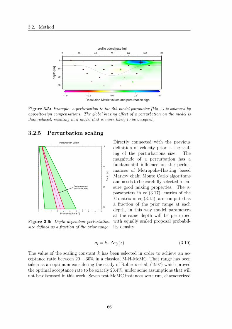
3.2. Method
−1.0 −0.5 0.0 0.5 1.0
Resolution Matrix values and perturbation sign
0
10
20
30
de
pth
[m
]0 20 40 60 80 100 120
profile coordinate [m]
-+
-
-
-
--
--
-
-- -
-
-
--
-+
-
-
+
+
Figure 3.5: Example: a perturbation to the 5th model parameter (big +) is balanced byopposite-sign compensations. The global biasing effect of a perturbation on the model isthus reduced, resulting in a model that is more likely to be accepted.
3.2.5 Perturbation scaling
0
10
20
30
De
pth
[m
]
0 1 2 3 4 5 6 7 8 9 10
P−velocity [km s−1]
Perturbation Width
Depth-dependent
perturbation width
Figure 3.6: Depth dependent perturbationsize defined as a fraction of the prior range.
Directly connected with the previousdefinition of velocity prior is the scal-ing of the perturbations size. Themagnitude of a perturbation has afundamental influence on the perfor-mances of Metropolis-Hasting basedMarkov chain Monte Carlo algorithmsand needs to be carefully selected to en-sure good mixing properties. The σi
parameters in eq.(3.17), entries of theΣ matrix in eq.(3.15), are computed asa fraction of the prior range at eachdepth, in this way model parametersat the same depth will be perturbedwith equally scaled proposal probabil-ity density:
σi = k ·∆vp(z) (3.19)
The value of the scaling constant k has been selected in order to achieve an ac-ceptance ratio between 20− 30% in a classical M-H-McMC. That range has beentaken as an optimum considering the study of Roberts et al. (1997) which provedthe optimal acceptance rate to be exactly 23.4%, under some assumptions that willnot be discussed in this work. Seven test McMC instances were run, characterized
66
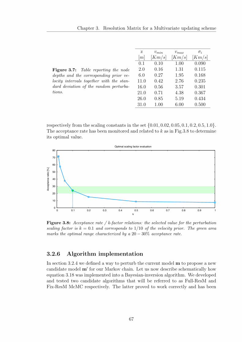
Chapter 3. Resolution Matrix for a Multivariate updating scheme
Figure 3.7: Table reporting the nodedepths and the corresponding prior ve-locity intervals together with the stan-dard deviation of the random perturba-tions.
z vmin vmax σi
[m] [Km/s] [Km/s] [Km/s]0.1 0.10 1.00 0.0902.0 0.16 1.31 0.1156.0 0.27 1.95 0.16811.0 0.42 2.76 0.23516.0 0.56 3.57 0.30121.0 0.71 4.38 0.36726.0 0.85 5.19 0.43431.0 1.00 6.00 0.500
respectively from the scaling constants in the set {0.01, 0.02, 0.05, 0.1, 0.2, 0.5, 1.0}.The acceptance rate has been monitored and related to k as in Fig.3.8 to determineits optimal value.
0
10
20
30
40
50
60
70
80
0 0.1 0.2 0.3 0.4 0.5 0.6 0.7 0.8 0.9 1
Acce
pta
nce
ra
tio
[%
]
k
Optimal scaling factor evaluation
Figure 3.8: Acceptance rate / k-factor relations: the selected value for the perturbationscaling factor is k = 0.1 and corresponds to 1/10 of the velocity prior. The green areamarks the optimal range characterized by a 20− 30% acceptance rate.
3.2.6 Algorithm implementation
In section 3.2.4 we defined a way to perturb the current model m to propose a newcandidate model m′ for our Markov chain. Let us now describe schematically howequation 3.18 was implemented into a Bayesian-inversion algorithm. We developedand tested two candidate algorithms that will be referred to as Full-ResM andFix-ResM McMC respectively. The latter proved to work correctly and has been
67

3.2. Method
utilized in the rest of this study while the first showed a number of flaws that ledto the decision not to carry on with its development.
3.2.6.1 Full-ResM updating scheme
1. Perform a DLS inversion to obtain a generalized inverse solution mdet (de-terministic solution Fig. 3.2.2)
2. Initialize the Markov Chain: the deterministic solution is set as startingmodel mdet = m .
3. Compute R the resolution matrix of the current model m
4. Generate a new trial model m′ perturbing the current model m
• At every iteration of the Markov process choose one of the n modelparameters randomly from a uniform distribution i ∈ u[1, n]
• Randomly perturb the velocity of the ith model parameter drawing froma Gaussian proposal probability density q(v′i|vi) (3.17)
• Compute and apply compensations to the other j = i parameters usingR as in eq(3.18)
5. Solve the forward problem: compute the estimated travel times dobs andevaluate the likelihood of the trial model Ltrial = p(dobs|m′)
6. Metropolis step: with the classical M-H algorithm randomly decide wetherto accept or reject the proposed move from m to m′ with the acceptingprobability α(m′|m) in eq.(1.26).
This schematized algorithm is the first intuitive way to modify a Metropolis-Hastings McMC including equation 3.18 in its updating scheme. A random per-turbation is applied to the current state m of the chain and compensations arecomputed from a functional g(R(m)) that yields information on the trade-off re-lations between model parameters, given by the resolution matrix that thereforeneeds to be computed at every iteration of the Markov chain.While proposing a new updating scheme for our modified M-H McMC we wantto preserve the stationarity of the stochastic process, therefore the reversibility(i.e. detailed-balance condition) must be preserved as well. With a non linearly-modified perturbation rule as eq.3.18 the reversibility is no longer guaranteed, sinceRij is computed at every iteration, and the transition probability is dependenton the current state of the chain. We chose to ignore this in a first attempt,assuming the modifications of Rij to be non-systematic, in the attempt to verify
68

Chapter 3. Resolution Matrix for a Multivariate updating scheme
DLS inversion
mdet
Initialize the MC
m=mdet
1.
2.
4.
- randomly chose the ith parameter to be
perturbed
- perturb the ith parameter
- compute and apply the compensations
to the other parameters
Generate a new model m’
5. Solve the forward problem and
compute the likelihood of m’
6. Metropolis algorithm accept/reject
3. Compute the resolution matrix of m
Figure 3.9: Scheme of the Full-ResM McMC algorithm: this updating scheme includesthe computation of the resolution matrix at every iteration of the Markov process.
if the stationarity would be maintained. Under this assumption the proposal ratiobecomes unity and the acceptance probability given by eq.1.26 would simplify tothe likelihood ratio (eq.1.29).
We tried to justify this assumption with a simple test: we run a McMC setting thelikelihood to a uniform distribution (Bodin and Sambridge, 2009), in this way webasically removed the data from the inverse problem and always accepted everyproposed move. From Bayes theorem we know that in this case the posterior distri-bution sampled in the process should be directly proportional to the chosen priordistribution. Should this not be case we would have proved false our assumption.
The posterior distributions recovered, show no correspondence with the prior dis-tribution that we selected, displayed here as the area delimited by the dashed redcurves. In particular the PDFs in Fig.3.10.a and .b show a clear shift to lower ve-locities suggesting a higher probability of making moves to lower velocities, whichcontrasts with the expectation of uniform distributions. A comparison with theprobability distributions obtained with the same test employing a classical M-Halgorithm (without Resolution matrix) shows how we would expect PDFs from a“healthy” Markov chain to behave (Fig.3.10.b and .c). In this case the probabilitydistributions appear to be simmetric respect to the middle of the prior area, andat depts where inverse nodes are located (red arrows) the distribution is uniform,
69

3.2. Method
(a)
0
10
20
30
De
pth
[m
]
0 1 2 3 4 5 6
P−velocity [km s−1]
PDF at profile position 25 (m)
0.0
0.5
1.0
Pro
ba
bili
ty
(b)
0
10
20
30
De
pth
[m
]
0 1 2 3 4 5 6
P−velocity [km s−1]
PDF at profile position 60 (m)
0.0
0.5
1.0
Pro
ba
bili
ty
Figure 3.10: Posterior distributions of the velocity displayed for profile position 25 (a)and 60 (b) obtained with the Full-ResM updating scheme. The area delimited by thedashed red curves corresponds to the prior.
(c)
0
10
20
30
De
pth
[m
]
0 1 2 3 4 5 6
P−velocity [km s−1]
PDF at profile position 25 (m)
0.0
0.5
1.0
Pro
ba
bili
ty
(d)
0
10
20
30
De
pth
[m
]
0 1 2 3 4 5 6
P−velocity [km s−1]
PDF at profile position 60 (m)
0.0
0.5
1.0
Pro
ba
bili
ty
PDFs for profile position 25 (c) and 60 (d) obtained with a classical M-H algo-rithm. The red arrows indicate the dephts at which inverse nodes are located.
70

Chapter 3. Resolution Matrix for a Multivariate updating scheme
therefore the prior has been correctly sampled. Such an outcome can be consid-ered as an heuristic proof of the fact that the transition kernel of our Full-ResMalgorithm is not symmetric as we assumed, thus a McMC algorithm implementedas above would not be able to correctly sample the desired posterior distribution.Even without giving a complete formulation of the transition probability betweenstates in a Markov chain characterized by the Full-ResM updating scheme, we cananyway state that it will be proportional to a term given by the functional g(R)n:
q(mn+1|mn) ∝ g(R)n (3.20)
where the index n signifies that mn is the nth state in the chain, mn+1 is the pro-posed state and g(R)n is the resolution-matrix functional of the nth model/state.The dependency of the transition probability from a term that is adapted at everystep of the Markov process leads to a state-dependent chain that does not convergeto the desired posterior distribution. The state-dependency of the Markov chainisn’t however the reason for the loss of convergence, since some drift-conditionscould be enforced in order to grant Harris-recurrence (Tweedie and Meyn, 1993,pp.466). It is instead the continuous adaptation of Rn, thus of the transition prob-ability, that makes for a non-converging process. With such a continuous adap-tation, the transition probabilities in a Markov chain can be expressed through afamily of transition kernels as:
Pr(mn+1|mn,mn−1, . . . ,m0, Kn, Kn−1, . . . , K0) = Pk(m,A) (3.21)
where Kn is the transition kernel at the nth iteration, depending on R(mn). Itthen possible that the probability to move from mn to mn+1 could depend fromthe whole history of the process and lead to the loss of convergence to a stationarydistribution. Roberts and Rosenthal (2007) proved that asymptotic convergencecan be however preserved under the diminishing adaptation condition:
limn→∞
sup ||PKn+1(m, ·)− PKn(m, ·)|| = 0 (3.22)
Here the requirement is that the adaptation at the nth iteration goes to 0 as ntends to infinity. Adaptive McMC are well known and can be easily found inliterature (e.g. Rosenthal in Brooks et al. (2011) chap.4) thus we will omit a moredetailed theoretical digression. A first possible solution to the loss of ergodicityand convergence could be the introduction of a time dependent scaling factor inthe transition probability to assure that its adaptation will diminish over time.
q(mn+1|mn) ∝ g(Rn) · d(n) (3.23)
In this way we would respect the condition (3.22) and save the convergence, buton the other hand we would lose at some point the trade-off relations carried by
71

3.2. Method
the functional g(R)n used to compute the compensation terms in our multivariateupdating scheme, which is the main purpose of this study.Discarding the option of introducing a scaling factor, the next possible solution canbe found dropping the practice of computing g(R)n at every iteration and evalu-ating it instead on batches of models of fixed length with a simple average (whichstill requires the computation of the resolution matrix at every iteration). In thisway we would not be adapting the transition probabilities at every iteration, andwithin each batch the convergence to an equilibrium distribution would be grantedby the central limit theorem. Now that with the introduction of batches we canavoid the issues connected with adaptation, we need to verify that a functionalg(Rb) could still be used to successfully compute the compensation terms in ourupdating scheme. In oder words, we know that the “exact” trade-offs are obtainedonly re-computing R at every step, but since that method has been proved unus-able our goal is now to prove that an approximation holds enough information.Provided that a batch has a “sufficient” length, the difference between the condi-tional distribution of each batch and the equilibrium distribution has to be small(zero for an infinite-length batch), hence we can assume that the R matrixes ofthe models in one batch are numerically not so dissimilar to each other and so isthe average resolution matrix Rb,q computed on that same batch. This assumptioncan be furthermore extended considering that an average on all the batches willalso yield this similarity:
Rb,q =1
b
bq∑n=b(q−1)+1
Rn (3.24)
where b is the number of models in a batch, Q is the number of batches and q isindexing them.
Rb,1 ≈ Rb,2 ≈ . . . ≈ Rb,Q ≈ 1
q
Q∑q=1
Rb,q (3.25)
The batch approach leaves us however with three main issues:
• the need to have “sufficiently” long batches to ensure stability
• the need to still evaluate R at every iteration
• the need to ensure that the diminishing adaptation condition (3.22) is re-spected
3.2.6.2 Fix-ResM updating scheme
The matrixes in eq.(3.25) are all Monte Carlo approximations of a functional of theresolution matrix, evaluations of a “quantity” that carries useful information on the
72
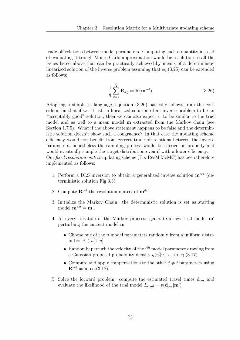
Chapter 3. Resolution Matrix for a Multivariate updating scheme
trade-off relations between model parameters. Computing such a quantity insteadof evaluating it trough Monte Carlo approximation would be a solution to all theissues listed above that can be practically achieved by means of a deterministiclinearized solution of the inverse problem assuming that eq.(3.25) can be extendedas follows:
1
q
Q∑q=1
Rb,q ≈ R(mdet) (3.26)
Adopting a simplistic language, equation (3.26) basically follows from the con-sideration that if we “trust” a linearized solution of an inverse problem to be an“acceptably good” solution, then we can also expect it to be similar to the truemodel and as well to a mean model m extracted from the Markov chain (seeSection 1.7.5). What if the above statement happens to be false and the determin-istic solution doesn’t show such a congruence? In that case the updating schemeefficiency would not benefit from correct trade off-relations between the inverseparameters, nonetheless the sampling process would be carried on properly andwould eventually sample the target distribution even if with a lower efficiency.Our fixed resolution matrix updating scheme (Fix-ResMMcMC) has been thereforeimplemented as follows:
1. Perform a DLS inversion to obtain a generalized inverse solution mdet (de-terministic solution Fig.3.3)
2. Compute Rdet the resolution matrix of mdet
3. Initialize the Markov Chain: the deterministic solution is set as startingmodel mdet = m .
4. At every iteration of the Markov process: generate a new trial model m′
perturbing the current model m
• Choose one of the n model parameters randomly from a uniform distri-bution i ∈ u[1, n]
• Randomly perturb the velocity of the ith model parameter drawing froma Gaussian proposal probability density q(v′i|vi) as in eq.(3.17)
• Compute and apply compensations to the other j = i parameters usingRdet as in eq.(3.18).
5. Solve the forward problem: compute the estimated travel times dobs andevaluate the likelihood of the trial model Ltrial = p(dobs|m′)
73
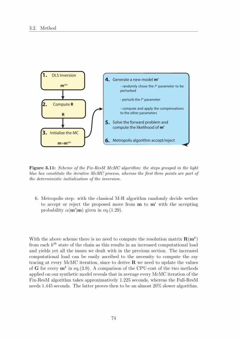
3.2. Method
DLS inversion
mdet
Compute R
R
Initialize the MC
m=mdet
1.
2.
3.
4.
- randomly chose the ith parameter to be
perturbed
- perturb the ith parameter
- compute and apply the compensations
to the other parameters
Generate a new model m’
5. Solve the forward problem and
compute the likelihood of m’
6. Metropolis algorithm accept/reject
Figure 3.11: Scheme of the Fix-ResM McMC algorithm: the steps grouped in the lightblue box constitute the iterative McMC process, whereas the first three points are part ofthe deterministic initialization of the inversion.
6. Metropolis step: with the classical M-H algorithm randomly decide wetherto accept or reject the proposed move from m to m′ with the acceptingprobability α(m′|m) given in eq.(1.29).
With the above scheme there is no need to compute the resolution matrix R(mk)from each kth state of the chain as this results in an increased computational loadand yields yet all the issues we dealt with in the previous section. The increasedcomputational load can be easily ascribed to the necessity to compute the raytracing at every McMC iteration, since to derive R we need to update the valuesof G for every mk in eq.(3.9). A comparison of the CPU-cost of the two methodsapplied on our synthetic model reveals that in average every McMC iteration of theFix-ResM algorithm takes approximatively 1.225 seconds, whereas the Full-ResMneeds 1.445 seconds. The latter proves then to be an almost 20% slower algorithm.
74

Chapter 3. Resolution Matrix for a Multivariate updating scheme
3.3 Tests and results
The Fix-ResM compensation scheme has been implemented, tests and results willbe presented and discussed in this section. So far we never explicitly gave anexpression of the compensation terms in eq.(3.18), using instead the functionalg(R). Four candidates were proposed 1:
a) g(R) =n∑
i =j
RijRii (3.27a)
b) g(R) =n∑
i =j
Rij
Rii
(3.27b)
c) g(R) =n∑
i =j
Rij (3.27c)
d) g(R) =n∑
i =j
Rij∑nj =i Rij
(3.27d)
which substituted in eq.(3.18) give the explicit equations for perturbation andcompensations to generate a proposed model
a) m′ = m+ uσiei − uσi
n∑i =j
RijRiiej (3.28a)
b) m′ = m+ uσiei − uσi
n∑i =j
Rij
Rii
ej (3.28b)
c) m′ = m+ uσiei − uσi
n∑i =j
Rijej (3.28c)
d) m′ = m+ uσiei − uσi
n∑i =j
Rij∑nj =i Rij
ej (3.28d)
In the next sections the four proposed transition kernels associated to the aboveequations have been tested in order to establish which resolution matrix functionalgives the optimal perturbation scheme. The letter notation “functional-a/b/c/d”will be used from now on with reference to the above four candidates expressed in
1the choice of these specific four candidates is to some extent heuristic: we will argue in theconclusions that more functionals could be proposed and investigated.
75
3.3. Tests and results
equations (3.27a/3.27d) with the addition of the “non-ResM” functional indicat-ing a classical perturbation scheme that makes no use of resolution-matrix basedcompensations.
3.3.1 Non-McMC tests
In order to compare the performances of the four functionals (3.27a/3.27d) whileexcluding the stochastic effects typically expected in a Monte Carlo process, anon-McMC test has been carried on as follows:
• The synthetic dataset is inverted with a McMC based on a classical Metropo-lis algorithm (no ResM-based perturbation scheme are used).
• 500 models are sub-sampled2 from the Markov chain ensemble obtaining anon-correlated subset.
• Each of the test models is perturbed iteratively using different methods:algorithm 2 displays a pseudo code.
• The models resulting from every perturbation with each method are mutuallycompared
• Statistical inference is performed in order to identify the optimal ResM-functional
Such a non-stochastic test finds its reason to be in the fact that a specific per-turbation can be applied, employing every method under exam, while controllingits magnitude and excluding other non reproducible effects. In this way specificproperties of each transition kernel can be examined. The magnitude of the per-turbations is 10% of the prior range given in eq.(3.11) at the depth zi of theperturbed node: v′i = vi + 0.1 ·∆vp(zi). This choice has been made clear in sec-tion 3.2.5. Considering that every model parameter is perturbed twice (once witha positive velocity increment, once with a negative one), our non-McMC test pro-duces five sets of 23000 perturbed models, one set for each transition kernel /functional being tested.
Misfit analysis The first of the properties compared to assess the performancesof the five perturbation schemes is the ability to propose “better” models, namelyto propose models whose misfit decreased after the perturbation proposed. Eval-uating the percentage of models characterized by lower misfit in Fig.3.12 the
2Subsampling a Markov chain at spacing k is the process of taking every kth element of aMarkov chain m1,m2, . . . obtaining a new Markov chain m1,mk+1,m2k+1, . . .
76
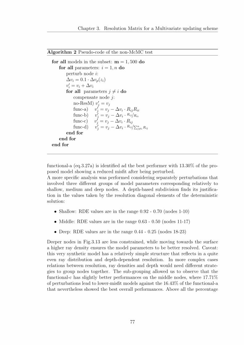
Chapter 3. Resolution Matrix for a Multivariate updating scheme
Algorithm 2 Pseudo-code of the non-McMC test
for all models in the subset: m = 1, 500 dofor all parameters: i = 1, n do
perturb node i:∆vi = 0.1 ·∆vp(zi)v′i = vi +∆vifor all parameters j = i do
compensate node j:no-ResM) v′j = vjfunc-a) v′j = vj −∆vi ·RijRii
func-b) v′j = vj −∆vi · Rij/Rii
func-c) v′j = vj −∆vi ·Rij
func-d) v′j = vj −∆vi · Rij/∑nj =i Rij
end forend for
end for
functional-a (eq.3.27a) is identified ad the best performer with 13.30% of the pro-posed model showing a reduced misfit after being perturbed.A more specific analysis was performed considering separately perturbations thatinvolved three different groups of model parameters corresponding relatively toshallow, medium and deep nodes. A depth-based subdivision finds its justifica-tion in the values taken by the resolution diagonal elements of the deterministicsolution:
• Shallow: RDE values are in the range 0.92 - 0.70 (nodes 1-10)
• Middle: RDE values are in the range 0.63 - 0.50 (nodes 11-17)
• Deep: RDE values are in the range 0.44 - 0.25 (nodes 18-23)
Deeper nodes in Fig.3.13 are less constrained, while moving towards the surfacea higher ray density ensures the model parameters to be better resolved. Caveat:this very synthetic model has a relatively simple structure that reflects in a quiteeven ray distribution and depth-dependent resolution. In more complex casesrelations between resolution, ray densities and depth would need different strate-gies to group nodes together. The sub-grouping allowed us to observe that thefunctional-c has slightly better performances on the middle nodes, where 17.71%of perturbations lead to lower-misfit models against the 16.43% of the functional-athat nevertheless showed the best overall performances. Above all the percentage
77
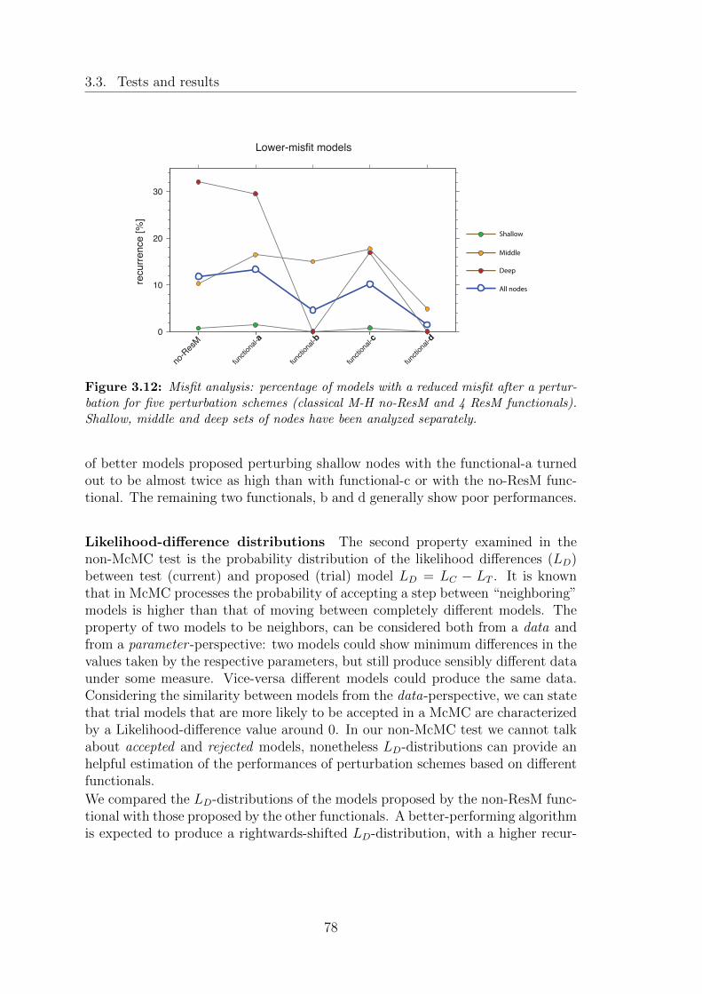
3.3. Tests and results
0
10
20
30
recu
rre
nce
[%
]Lower-misfit models
no-R
esM
func
tiona
l-a
func
tiona
l-b
func
tiona
l-c
func
tiona
l-d
Shallow
Middle
Deep
All nodes
Figure 3.12: Misfit analysis: percentage of models with a reduced misfit after a pertur-bation for five perturbation schemes (classical M-H no-ResM and 4 ResM functionals).Shallow, middle and deep sets of nodes have been analyzed separately.
of better models proposed perturbing shallow nodes with the functional-a turnedout to be almost twice as high than with functional-c or with the no-ResM func-tional. The remaining two functionals, b and d generally show poor performances.
Likelihood-difference distributions The second property examined in thenon-McMC test is the probability distribution of the likelihood differences (LD)between test (current) and proposed (trial) model LD = LC − LT . It is knownthat in McMC processes the probability of accepting a step between “neighboring”models is higher than that of moving between completely different models. Theproperty of two models to be neighbors, can be considered both from a data andfrom a parameter -perspective: two models could show minimum differences in thevalues taken by the respective parameters, but still produce sensibly different dataunder some measure. Vice-versa different models could produce the same data.Considering the similarity between models from the data-perspective, we can statethat trial models that are more likely to be accepted in a McMC are characterizedby a Likelihood-difference value around 0. In our non-McMC test we cannot talkabout accepted and rejected models, nonetheless LD-distributions can provide anhelpful estimation of the performances of perturbation schemes based on differentfunctionals.
We compared the LD-distributions of the models proposed by the non-ResM func-tional with those proposed by the other functionals. A better-performing algorithmis expected to produce a rightwards-shifted LD-distribution, with a higher recur-
78
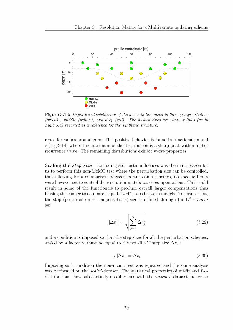
Chapter 3. Resolution Matrix for a Multivariate updating scheme
0
10
20
30
de
pth
[m
]
0 20 40 60 80 100 120
profile coordinate [m]
Shallow
Middle
Deep
Figure 3.13: Depth-based subdivision of the nodes in the model in three groups: shallow(green) , middle (yellow), and deep (red). The dashed lines are contour lines (as inFig.3.3.a) reported as a reference for the synthetic structure.
rence for values around zero. This positive behavior is found in functionals a andc (Fig.3.14) where the maximum of the distribution is a sharp peak with a higherrecurrence value. The remaining distributions exhibit worse properties.
Scaling the step size Excluding stochastic influences was the main reason forus to perform this non-McMC test where the perturbation size can be controlled,thus allowing for a comparison between perturbation schemes, no specific limitswere however set to control the resolution-matrix-based compensations. This couldresult in some of the functionals to produce overall larger compensations thusbiasing the chance to compare “equal-sized” steps between models. To ensure that,the step (perturbation + compensations) size is defined through the L2 − normas:
||∆v|| =
√ n∑j=1
∆v2j (3.29)
and a condition is imposed so that the step sizes for all the perturbation schemes,scaled by a factor γ, must be equal to the non-ResM step size ∆vi :
γ||∆v|| != ∆vi (3.30)
Imposing such condition the non-mcmc test was repeated and the same analysiswas performed on the scaled -dataset. The statistical properties of misfit and LD-distributions show substantially no difference with the unscaled -dataset, hence no
79

3.3. Tests and results
0
2
4
6
8
10
12
14
-100 -80 -60 -40 -20 0
Re
cu
rre
nce
[%
]
LC-LT
LD-distribution
no-ResMfunc-a
(a) functional-a
0
2
4
6
8
10
12
14
-100 -80 -60 -40 -20 0
LC-LT
LD-distribution
no-ResMfunc-b
(b) functional-b
0
2
4
6
8
10
12
14
-100 -80 -60 -40 -20 0
Re
cu
rre
nce
[%
]
LC-LT
LD-distribution
no-ResMfunc-c
(c) functional-c
0
2
4
6
8
10
12
14
-100 -80 -60 -40 -20 0
LC-LT
LD-distribution
no-ResMfunc-d
(d) functional-d
Figure 3.14: LD-distributions produced by the four functional under exam comparedwith the distribution obtained with the no-ResM functional (in red). A better-performingalgorithm is expected to produce a rightwards-shifted LD-distribution, with a higher re-currence for values around zero.
80

Chapter 3. Resolution Matrix for a Multivariate updating scheme
influence on the performances of the tested updating schemes is to be expecteddue to inherent differences in the proposed step sizes.
3.3.2 Fix-ResM McMC test
The testing phase to compare the four different functionals (3.27a/3.27d) pro-ceeded with the analysis of the ensemble properties of Markov chains obtainedemploying the Fix-ResM McMC each one characterized by a different functional.For the non-McMC test we started analyzing misfit and LD-distributions, we willproceed similarly with the only difference that in a McMC contest we can nowconsider the acceptance rate instead of it’s misfit-based estimator we used in theprevious section (Fig.3.12).
no-ResM func-a func-b func-c func-d24.50 27.71 17.17 24.40 27.76
Table 3.3.1: Acceptance rates [%] relative to Markov chains characterized by the use ofthe four functionals plus the “classical” non-ResM McMC.
Acceptance rates The no-ResM McMC we are looking to improve accepted24.50% of the proposed models, an higher acceptance rate is shown in the Markovchains based on the functionals-a and d with a value around 27.7% (table.3.3.1).The functional-b based McMC results in a drastic decrease in the acceptance ratewhereas the remaining functional-c shows a value comparable with the “classical”algorithm.
Likelihood-difference distributions Following the same procedure applied forthe non-McMC tests the likelihood differences were analyzed confirming the behav-ior observed in Fig.3.14 which highlighted the functional-a as the best candidateable to shift part of the original non-ResM distribution (in red in Fig.3.15) toobtain a sharper peak around zero. Acceptance rate values and LD-distributionsshow a quantitative agreement while pointing out functionals-a and d as the mostappropriate candidates.A good qualitative and quantitative agreement is found also comparing LD -distributions in Fig.3.15, proving the ability of the non-stochastic tests to indepen-dently evaluate and foresee some of the statistic properties of the Markov chains.An exception should be made for functional-d (Fig.3.14.d and 3.15.d) that displaysan incongruence in the behavior of its LD-distributions. A possible explanationcould lie in the nature itself of our non-McMC test: we decided to remove stochasticinfluences defining a fixed perturbation magnitude (10% of the prior range) which
81

3.3. Tests and results
0
2
4
6
8
10
12
14
-100 -80 -60 -40 -20 0
LC-LT
LD-distribution ALL
no-ResMfunc-a
Re
cu
rre
nce
[%
]
(a) functional-a
0
2
4
6
8
10
12
14
-100 -80 -60 -40 -20 0
LC-LT
LD-distribution ALL
no-ResMfunc-b
(b) functional-b
0
2
4
6
8
10
12
14
-100 -80 -60 -40 -20 0
LC-LT
LD-distribution ALL
no-ResMfunc-c
(c) functional-c
0
2
4
6
8
10
12
14
-100 -80 -60 -40 -20 0
LC-LT
LD-distribution ALL
no-ResMfunc-d
(d) functional-d
Figure 3.15: Comparison of the LD-distributions of Markov chains based on the Fix-ResM updating scheme. In red the reference distribution relative to the “classical”McMC.
might have caused the functional-d to produce compensations that resulted quiteoften in “worse” proposed models (i.e. LD-distribution less-peaked around zero).Testing the same functional in a McMC allows instead the perturbation magni-tudes to be randomly selected on a continuous set, thus eliminates this behaviorobserved in the non-stochastic test. In other words, while our non-McMC test pro-vides a useful tool to compare the behaviors of different perturbation schemes, oneshould be aware that the statistical population analyzed is way more limited thanthat of an actual McMC, thus could be subject to slightly different outcomes. Moreattention could be dedicated to this point in future studies. Anyway the resultsobtained with the non-McMC tests as we described them, seem to ensure a goodlevel of reliability and help in the analysis of the different functionals proposed.
Mixing properties The third of the three criteria we outlined in section 3.1.2states that a Markov chain is better if it allows a faster sampling of the state
82

Chapter 3. Resolution Matrix for a Multivariate updating scheme
space. Instead of computing an estimate of the expectation (eq.3.3) a graphicalevaluation of the sampling speed of a Markov chain can be conveniently achievedwith a trace plot of the values taken by parameters or functionals of the chainitself. Two model parameters were selected, corresponding to one superficial node(depth 0.1m) and a deep node (depth 25m), the trace plots report the P-velocityvalue assumed by the parameters at each McMC step for a total of 3000 iterations.The non-ResM chain (uppermost row of Fig.3.16) displays a good mixing for thebottom node: there is a good balance between the frequency of accepted moves(appropriate acceptance rate) and the change in the velocity values (appropriatestep size). On the contrary the upper node has poor mixing properties with alow frequency of accepting moves (low acceptance rate) and relatively big changes.One possible interpretation of this behavior could consider it a consequence ofa still sub-optimal scaling of the perturbation size, despite the depth-dependentperturbation scaling applied (see section 3.2.5). A second, non-complementaryway to interpret the behavior of the shallow nodes is to observe that they arerelatively well-constrained, even small perturbations have a large impact on thedata, which makes perturbations less likely to ba accepted. This group of nodes isthe one where we expect the most improvement. Applying our resolution matrix-based updating scheme we can compare the different effects of the four testedfunctionals on the mixing properties of the resulting Markov chains:
a) The upper node shows an improved mixing, the frequency of accepted moveshas increased together with the step size. No substantial improvement canbe visually appreciated for the deep node.
b) Strongly improved mixing can be observed for the shallow node, on the otherhand there’s a drastic decrease of performance regarding the deeper nodewhere we observe a high frequency of accepting small velocity changes re-sulting in a inefficient sampling.
c) We observe a strongly improved mixing for the shallow node, and a slightdecrease in sampling efficiency for the lower nodes.
d) The shallow node exhibits poor mixing ability at a level comparable with thenon-ResM chain. The deep node instead seem to improve the samplingperformances.
Summarizing what observed so far, the functional-a appears to improve the mixingability for parameters located at all depths while the other functionals seem to haveworse performances either for deep (functional-b and c) or for surface parameters(functional-d). Similarly, also trace plots for mid-depth parameters have beenanalyzed, verifying that improvements to the mixing properties can be observed
83
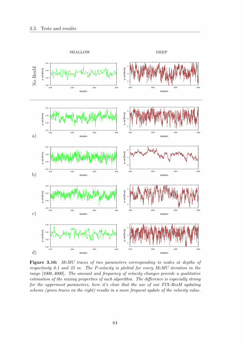
3.3. Tests and results
shallow deep
NoResM
0.32
0.33
0.34
0.35
p−
vel [K
m/s
]
1000 2000 3000 4000
iteration
2
3
4
p−
ve
l [K
m/s
]
1000 2000 3000 4000
iteration
a)
0.32
0.33
0.34
0.35
p−
vel [K
m/s
]
1000 2000 3000 4000
iteration
2
3
4
p−
ve
l [K
m/s
]
1000 2000 3000 4000
iteration
b)
0.32
0.33
0.34
0.35
p−
vel [K
m/s
]
1000 2000 3000 4000
iteration
2
3
4
p−
ve
l [K
m/s
]
1000 2000 3000 4000
iteration
c)
0.32
0.33
0.34
0.35
p−
vel [K
m/s
]
1000 2000 3000 4000
iteration
2
3
4
p−
ve
l [K
m/s
]
1000 2000 3000 4000
iteration
d)
0.32
0.33
0.34
0.35
p−
vel [K
m/s
]
1000 2000 3000 4000
iteration
2
3
4
p−
ve
l [K
m/s
]
1000 2000 3000 4000
iteration
Figure 3.16: McMC traces of two parameters corresponding to nodes at depths ofrespectively 0.1 and 25 m. The P-velocity is plotted for every McMC iteration in therange [1000, 4000]. The amount and frequency of velocity changes provide a qualitativeestimation of the mixing properties of each algorithm. The difference is especially strongfor the uppermost parameters, here it’s clear that the use of our FIX-ResM updatingscheme (green traces on the right) results in a more frequent update of the velocity value.
84

Chapter 3. Resolution Matrix for a Multivariate updating scheme
from all the functionals at a comparable level thus we won’t report any trace plotfor such nodes.
To support quantitatively what has been qualitatively deduced from the McMCtrace plots we can estimate values of eq.(3.3) by means of the step size given ineq.(3.29) as:
E∥∆v∥ =
√ 1
N
N∑i=1
(n∑
j=1
∆v2j
)(3.31)
where N is the number of the steps attempted during the Markov process and nthe number of model parameters. Such estimator provides a quantification of themixing ability of a Markov chain in a form that resembles a quadratic mean of thestep sizes of a chain. Evaluations of eq.(3.31) are reported in table 3.3.2:
shallow middle deepno-ResM 0.007280 0.052309 0.192393
functional-a 0.011934 0.072848 0.197953functional-b 0.009932 0.061792 0.035045functional-c 0.011876 0.081926 0.116228functional-d 0.008493 0.065230 0.236194
Table 3.3.2: Evaluations of eq. 3.31 computed for each functional.
Here the functional-a proves once more to lead to a Markov chain with improvedmixing properties at all depths, especially for shallow, highly constrained modelparameters. It’s evident that also the functional-d improves the mixing at alldepths especially for the deepest nodes where it performs better than the othercandidates.
Choice of functional-a Considering the outcome of the tests conduced weselected functional-a as the best of the examined candidates. If this choice isclear considering functionals-b and c, the last option d appears to perform on asimilar level, then a justification is needed. While “global” indicators as acceptancerate and LD-distributions gave substantially similar results for both a and d, thegraphical and quantitative analysis of mixing show how the two functionals performdifferently. Functional-d leads to an improved mixing for all the nodes but thegain is more focused on deep nodes, thus on less constrained model parameters. Inthe framework of seismic tomography it appears however more desirable to obtaina better mixing of highly constrained parameters. From a sampling point of viewimproving the mixing of strongly constrained nodes translates in an increased
85

3.3. Tests and results
acceptance of moves involving perturbations to parameters that have a strongerinfluence on the likelihood.Furthermore as expected “better” sampling leads to a reduced variance of theposterior estimates (eq.3.2), in other words the PDFs obtained from better chainsare supposed to have smaller variance after the same number of iterations. Figure3.17.a shows that the difference of the variances between the functional-a-chainand the no-ResM-chain is basically only negative, contrary to the other maps thatshow also increases in the variance. This behavior is quantitatively limited for thesimple test model utilized but is expected to become more evident for other morecomplex models.
0.0
Variance difference [km/s]
0
10
20
30
depth
[m
]
0 20 40 60 80 100 120
profile coordinate [m]
(a)
0.0
Variance difference [km/s]
0
10
20
30
depth
[m
]
0 20 40 60 80 100 120
profile coordinate [m]
(b)
0.0
Variance difference [km/s]
0
10
20
30
depth
[m
]
0 20 40 60 80 100 120
profile coordinate [m]
(c)
0.0
Variance difference [km/s]
0
10
20
30
depth
[m
]
0 20 40 60 80 100 120
profile coordinate [m]
(d)
Figure 3.17: Variance difference maps between the four functionals and the NoResMMcMC. Functional-a is the only that displays only a variance reduction.
86

Chapter 3. Resolution Matrix for a Multivariate updating scheme
3.3.3 Bayesian seismic tomography with the Fix-ResMMcMCalgorithm
Functional-a, expressed in eq.3.27a, was selected as the best of the proposed can-didates, this choice was based on the criteria introduced in section 3.1.2, andinvestigated with non-stochastic and McMC tests.We run the fix-ResM McMC algorithm fitted-out with the chosen functional on adesktop workstation equipped with an eight-core Intel(R) Core(TM) i7-2600 CPU@ 3.40GHz for 20 days. A total of ≈ 3.63M iterations produced a set of 1.0Mmodels, every 10th accepted model has been stored as state of the Markov chain.Thinning the chain allows to ease the computational load in the analysis phaseof the statistical ensemble avoiding to deal with an unnecessary huge number ofhighly correlated models. No burn in was needed since, with the choice of the DLS-solution as initial model state, the Markov chain was initialized near the center ofthe equilibrium distribution.
0 1 2 3 4 5 6
PDF at profile position 25 (m)
0.0
0.5
1.0
Pro
ba
bili
ty
0
10
20
30
De
pth
[m
]
0 1 2 3 4 5 6
P−velocity [km s ]−1
PDF at profile position 60 (m)
Mean modelStandard deviationDeterministic solutionSynthetic model
Figure 3.18: Vertical cross sections of the posterior distribution at profile position 25and 60 m. displayed together with the mean model, DLS deterministic solution andsynthetic “real” values. The thin pink lines mark the confidence interval given by ± onestandard deviation.
87
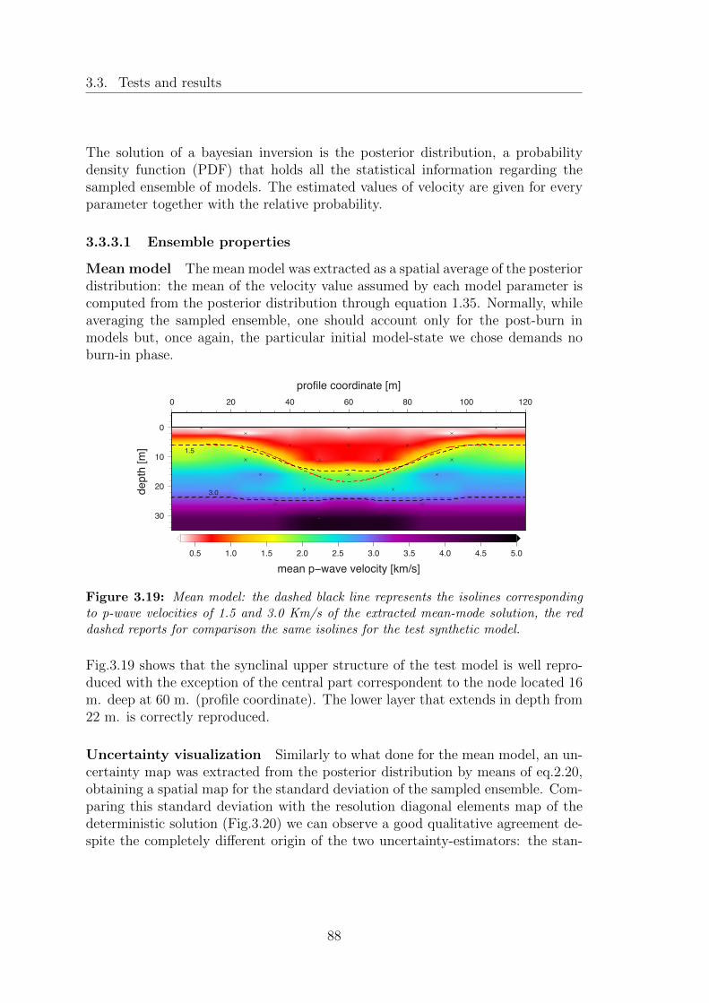
3.3. Tests and results
The solution of a bayesian inversion is the posterior distribution, a probabilitydensity function (PDF) that holds all the statistical information regarding thesampled ensemble of models. The estimated values of velocity are given for everyparameter together with the relative probability.
3.3.3.1 Ensemble properties
Mean model The mean model was extracted as a spatial average of the posteriordistribution: the mean of the velocity value assumed by each model parameter iscomputed from the posterior distribution through equation 1.35. Normally, whileaveraging the sampled ensemble, one should account only for the post-burn inmodels but, once again, the particular initial model-state we chose demands noburn-in phase.
0.5 1.0 1.5 2.0 2.5 3.0 3.5 4.0 4.5 5.0
mean p−wave velocity [km/s]
0
10
20
30
de
pth
[m
]
0 20 40 60 80 100 120
profile coordinate [m]
1.5
3.0
Figure 3.19: Mean model: the dashed black line represents the isolines correspondingto p-wave velocities of 1.5 and 3.0 Km/s of the extracted mean-mode solution, the reddashed reports for comparison the same isolines for the test synthetic model.
Fig.3.19 shows that the synclinal upper structure of the test model is well repro-duced with the exception of the central part correspondent to the node located 16m. deep at 60 m. (profile coordinate). The lower layer that extends in depth from22 m. is correctly reproduced.
Uncertainty visualization Similarly to what done for the mean model, an un-certainty map was extracted from the posterior distribution by means of eq.2.20,obtaining a spatial map for the standard deviation of the sampled ensemble. Com-paring this standard deviation with the resolution diagonal elements map of thedeterministic solution (Fig.3.20) we can observe a good qualitative agreement de-spite the completely different origin of the two uncertainty-estimators: the stan-
88

Chapter 3. Resolution Matrix for a Multivariate updating scheme
dard error map is in fact a posterior estimate obtained from the sampled modelswhile the RDE map is computed on the last iteration solution of the DLS inversion.A fundamental difference lies however between these two methods of uncertaintyvisualiztion: the bayesian approach allows a quantitative estimation of the uncer-tainty, i.e. a measure of confidence. On the other hand the RDE map only providesqualitative values, a relative measure of where the resolution is higher, dependingon the damping values utilized in the deterministic inversion process. Figure 3.20.aallows a quantification of the uncertainty that characterizes the mean model: theshallow portion with velocities ≤ 1.5 Km/s is associated with a standard deviationup to 0.1 Km/s, while the bottom part with higher velocities shows uncertainties≥ 0.5 Km/s, value that corresponds to the isoline of 3.0 Km/s in Fig.3.19.
0.00 0.25 0.50 0.75 1.00
standard deviation [km/s]
0
10
20
30
dept
h [m
]
0 20 40 60 80 100 120
(a) (b)
0.1
0.5
0.00 0.25 0.50 0.75 1.00
resolution
0 20 40 60 80 100 120
profile coordinate [m]
0.5
0.7
Figure 3.20: Standard deviation map obtained from the posterior probability distribu-tion (a) and map of the resolution diagonal elements obtained from the last iteration ofthe DLS solution (b). For the resolution map, the contour lines are defined basing onthe node subdivision of Pag.77.
Useful practice to highlight parameters affected by relatively higher uncertaintiesis a relative error map defined by means of the standard deviation and the meanmodel maps. This map reported in Fig.3.21 makes possible to notice that thecentral area of the model (the portion of the synclinal structure deeper than 6m.) is probably affected by errors relatively high for that depth. Comparing themean model (Fig.3.19) with the synthetic model (Fig.3.2) one can verify that theestimated mean velocity value of the two nodes located at 11 m depth and profilepositions 50 and 70 m is actually lower than the synthetic-real value, while theunderlying node has an estimated mean velocity higher than the synthetic value.
89

3.4. Discussion and Conclusions
Figure 3.21:Relative error map:the black dashed linemarks the contours of10% relative standarderror, the red contoursreport for comparisonthe main structural fea-tures of the syntheticmodel.
0 25 50 75 100
Relative standard error [%]
0
10
20
30
de
pth
[m
]
0 20 40 60 80 100 120
profile coordinate [m]
10
101.5
3.0
3.4 Discussion and Conclusions
Besides the application of our resolution-matrix-based multivariate updating schemeto a synthetic dataset, as reported in section 3.3.3, we employed a classical M-HMcMC for the inversion of the same dataset. Both Markov chains were left runninguntil each one accepted a total of 1 Million of models. A recap of some parametersfor the two inversions is reported in Table 3.4.1.
no-ResM fix-ResMAccepted models 1 Mil. 1 Mil.Number of Iterations 4080293 3627027Runtime 554.5 hrs. 497.2 hrs.Acceptance rate 24.508 % 27.571 %
Table 3.4.1: Performance comparison between a classical M-H McMC and our Fix-ResM algorithm.
We observed that in the Fix-ResM Markov Chain the acceptance ratio increasedby about 3% compared to the inversion that makes use of a classical updatingscheme. On the usual time scale of bayesian inversions this can translate in areduction of the computation time that in the case we illustrated corresponds to≈ 10%.The McMC-trace analysis shows that our multivariate updating scheme results inwider and more frequent movement of the parameters values. In addiction theincrease in the acceptance ratio without diminishing the perturbation size leads usto the conclusion that, using such a ResM-based perturbation scheme, a McMCwill have better mixing properties, thus will sample the model space with higherefficiency.
90

Chapter 4
Discussion and conclusions
4.1 Achievements
The research we conducted in this project aimed to face some of the major issuesof geophysical inversion processes such as the quantification of the underdeter-mination that affects inverse solutions, the choice of a parametrization, in termsof both node density and geometry, the determination of some inversion parame-ters as damping and smoothing. These issues have been tackled with a Bayesianapproach, through the implementation of Markov chain Monte Carlo inversion al-gorithms. The intrinsic intensive computational load that characterizes this familyof sampling methods demands for optimized procedures. We focused our atten-tion on two different optimization strategies that have been applied respectivelyon transdimensional and non-transdimensional inversion schemes: parallelizationand optimization of transition kernels.
Trandimensional McMC We have proved that despite the intrinsic serial na-ture of Markov chains, it is possible to exploit the benefits offered by parallelcomputing with a trivial implementation that requires minimal coding effort. Thepractice of running independent parallel Monte Carlo sampling processes showedits effectiveness together with the inversion algorithm we developed also thanks tothe extremely limited portion, as small as 0.5%, of models discarded within theburn-in phase. This was achieved initializing the Markov processes with a deter-ministic DLS solution, however even chains initialized with fairly simple velocitymodels, as linear gradients, produced limited burn-in phases. This results in analmost linear dependence between speedup and CPU/cores involved in the paral-lelization, thus in the opportunity to make use of a massive parallelization to gaina more efficient sampling.
The use of a staggered-grid approach in addition to independent parallel transdi-
91

4.2. Future directions
mensional Markov chains allowed to recover more structural details and smootherreference solution models than a deterministic DLS inversion. The mean modelmap of the Salzach valley extracted from the sampled ensemble exhibits a high levelof compatibility with the refraction-reflection (RRTT) and with the full-waveformsolutions of Bleibinhaus and Hilberg (2012) despite the use of information carriedby first-breaks traveltimes only. The higher computation cost of this Bayesianapproach seems therefore to be repaid not only by the possibility to provide aquantitative estimation of the modeling errors, but also from solution models ableto recover smaller structural details.
Resolution-Matrix-based updating scheme We developed a multivariateupdating scheme that utilizes the Model Resolution Matrix to propose trial mod-els with a higher probability of acceptance. The Bayesian inversion algorithmwe developed is based on the Metropolis-Hastings scheme, a trial model is hereproposed applying a normal-distributed main perturbation to one parameter ofthe current model-state, followed by compensations applied to all the remainingmodel parameters. Such compensations, computed by means of a functional ofthe Resolution Matrix are aimed to reduce the global biasing effect of the mainperturbation. The resulting updating scheme proved to lead to better performingMarkov chains in terms of improved mixing properties, reduced variance of thesampled ensemble, increased acceptance rate.
While multivariate proposal schemes find their main limitation in the difficulty topropose trial models yielding a high acceptance probability, we proved that theModel Resolution Matrix can be successfully utilized to overcome such issue.
4.2 Future directions
In our quest for optimal McMC inversion algorithms we would like to focus onsome of the aspects of the algorithms we developed, that could have room forfurther improvement.
4.2.1 Voronoi parametrization
The node-based parametrization and the interpolation scheme characterizing thesimulr16 code, allow for the reconstruction of complex structures with a relativelylimited number of model parameters. The consequent restrained cardinality ofthe model space is undoubtedly a benefit for the Bayesian inversion algorithmspresented in this work since the runtime needed to sample a model space increaseswith the number of its elements.
92

Chapter 4. Discussion and conclusions
However a downside of this model parametrization is the fact that transdimen-sional McMC inversions won’t fully benefit from the Occam’s razor principle thatnaturally characterizes this family of McMC methods. A model parametrizationdefined through a precisely limited set of nodes, with defined positions could some-how appear as a contradiction with the transdimensional approach that would onthe contrary prefer to have total freedom in the choices of position and number ofinverse parameters during the sampling process. A well diffused parametrizationstrategy that satisfies these characteristics is based on the Voronoi tessellation,some of the latest and most notable applications on seismic tomographic inver-sion can be found in Bodin and Sambridge (2009); Bodin et al. (2012). ThroughVoronoi polygons, or Delaunay triangles one could parametrize models allowingfor non-discretized node positions, thus independent from underlying pre-definedgridded locations. An interesting direction of study could be the comparison ofthe performances of McMC tomographic inversions, within the simul framework,associated to different parametrization strategies such as the mentioned Voronoiand Delaunay, considering as well different interpolation algorithms.
4.2.2 Reflection-refraction seismics
A Bayesian approach could be extended to the analysis of reflection data as well.Simulr16 provides already provides established tools for the deterministic inver-sion of such refraction-reflection data sets. Reflecting interfaces are treated insimulr16 with a method of Bleibinhaus (2003), based on a nearest neighbor in-terpolation. Reflectors are parameterized as splines on separate grids, and thecorresponding velocity discontinuities arise from interrupting the velocity interpo-lation. That allows for defining smooth, curved reflector surfaces with very fewparameters. The modeling of reflectors in this method is highly flexible: they canbe floating, i.e. without connection to the velocity field, or they can be disconti-nuities. Also, because the parameterization is not layer-based, reflectors must notspan the entire model, nor have they to be sub-horizontal. All the parameters in-volved in the definition of reflectors could be treated as unknowns within a McMCinversion process: depths, coordinates as well as the number of nodes that define areflector could be therefore described in terms of posterior distributions expressingthe probability for an interface to have certain characteristics (i.e. shape, depth...).This method would require the formal definition of prior distributions and likeli-hood functions providing an appropriate probabilistic description of the quantitiesconnected with reflectors.
93

4.2. Future directions
4.2.3 Combined functionals
For our fix-ResM updating scheme we proposed and compared four different func-tionals of the Model Resolution Matrix, analyzing their performances both in aMcMC environment and non-stochastic tests. From the results we obtained it ap-pears that the performances of the tested functionals are partially dependent onthe respective RDE value of each inverse parameter: while the mixing properties ofhighly constrained nodes (i.e. with RDE values approaching the unity) shows thehighest increment with one functional, another leads to an optimal mixing for lessconstrained parameters. We reckon that more functionals should be proposed andtested seeking for an overall “best performer”. In the absence of a clear optimalchoice a promising strategy appears to be the combination of the best functionalson RDE basis. One could make use of multiple functionals at the same time: let’sassume that three functionals α, β, γ have been identified as the most appropriaterespectively for highly, medium, and poorly-constrained inversion parameters. Inour fix-ResM algorithm, a perturbation of a highly-constrained parameter wouldbe followed by compensations computed using the α-functional. Similarly, pertur-bations of medium-constrained nodes would be associated to β-functional compen-sations and γ for the highly-constrained nodes. This approach brings however thequestion “how to define highly/middle/low constrained nodes?”. Thresholds wouldneed to be defined for the RDE values characterizing each of the groups, with theconsequent issues connected to this arbitrary choice. An alternative strategy couldbe a continuous approach that makes use of all the three functionals at once, as-signing them RDE-dependent weighting factors, allowing therefore for “smoothedboundaries” between parameter groups. Along these lines a trial model would beproposed with a slightly different version of (3.18) as:
m′ = m+ uσiei − uσi
n∑j =i
[wαgα(Rij) + wβgβ(Rij) + wγgγ(Rij)] ej (4.1)
where wα, wβ, wγ are weighting factors such that wα +wβ +wγ = 1, proportionalto the RDE value Rii of the i-node being perturbed. In this way one could obtainan updating scheme where the resolution-matrix-based compensations are alwayscomputed with an optimal functional.
4.2.4 Transdimensional McMC and Resolution Matrix
So far we treated transdimensional and fixed-dimension McMC algorithms as twodistinctly separated groups. The two updating schemes we implemented are at theactual stage non compatible with each other, it appears therefore of high interest toresearch the feasibility of utilizing the Resolution Matrix to produce compensationsin a multivariate updating scheme within a transdimensional framework.
94

Chapter 4. Discussion and conclusions
4.2.5 A unified approach
For the McMC-optimization perspective we adopted so far it is of fundamentalimportance to join all the possible strategies that could contribute to the genera-tion of optimal Markov chains, to obtain a fast and reliable working tool for theBayesian inversion of seismic tomographic data. Multiple instances of the samplershould run in parallel on independent cores/CPUs, the forward solver should beparallelized over the sources, and a staggered grid approach should be used incombination with the simulr16 built-in node-parametrization. In case a differentparametrization would be used, based for instance on Voronoi or Delaunay tessel-lation, the staggered approach could be avoided. One should initialize the Markovprocesses with a deterministic solution model in order to sensibly shorten or eveneliminate the need to throw away models in the burn-in.The most crucial problem in the application of McMC methods lies in the op-timization of the algorithms, in order to obtain a maximum reduction of thecomputation-time, given the limits typically imposed by the available time andhardware resources. It is therefore desirable that all the established (and compati-ble) methods, which could contribute to increase efficiency and quality of Bayesianinversion algorithms, will be employed together in a framework offered by an highlyparallelized code whose forward and inverse routines are optimized to run on clus-ters of variable dimensions.
95

4.2. Future directions
96

Bibliography
Ajo-Franklin, J., Urban, J., and Harris, J. (2006). Using resolution-constrainedadaptive meshes for traveltime tomography. Journal of Seismic Exploration,14:371–392.
Bleibinhaus, F. (2003). Entwicklung einer simultanen refraktions- und re-flexionsseismischen 3D-Laufzeittomographie mit Anwendung auf tiefenseismis-che TRANSALP-Weitwinkeldaten aus den Ostal- pen. PhD thesis, Ludwig-Maximilians-Universitat Munchen.
Bleibinhaus, F. and Gebrande, H. (2006). Crustal structure of the eastern alpsalong the transalp profile from wide-angle seismic tomography.
Bleibinhaus, F. and Hilberg, S. (2012). Shape and structure of the salzach val-ley, austria, from seismic traveltime tomography and full waveform inversion.Geophysical Journal International, 189(3):1701–1716.
Bleibinhaus, F., Hilberg, S., and Stiller, M. (2010). First results from a seismicsurvey in the upper salzach valley, austria. Austrian Journal of Earth Sciences,103(2):28–32.
Bodin, T. and Sambridge, M. (2009). Seismic tomography with the reversible jumpalgorithm. Geophysical Journal International, 178(3):1411–1436.
Bodin, T., Sambridge, M., Rawlinson, N., and Arroucau, P. (2012). Transdimen-sional tomography with unknown data noise. Geophysical Journal International,189(3):1536–1556.
Bohm, G., Galuppo, P., and Vesnaver, A. (2000). 3d adaptive tomography usingdelaunay triangles and voronoi polygons. Geophysical Prospecting, 48(4):723–744.
Brockwell, A. E. (2006). Parallel markov chain monte carlo simulation by pre-fetching. Journal of Computational and Graphical Statistics, 15(1):246–261.
97

Bibliography
Brooks, S., Gelman, A., Jones, G. L., Meng, X.-L., and Rosenthal, J. S. (2011).Handbook of Markov Chain Monte Carlo. Chapman and Hall/CRC.
Campillo, F., Rakotozafy, R., and Rossi, V. (2009). Parallel and interactingmarkov chain monte carlo algorithm. Mathematics and Computers in Simu-lation, 79(12):3424–3433.
Debski, W. (2010). Seismic tomography by monte carlo sampling. Pure and AppliedGeophysics, 167(1-2):131–152.
Del Moral, P. (1996). Non linear filtering: Interacting particle solution. MarkovProcesses and Related Fields, 2(4):555–580.
Duijndam, A. J. W. (1988a). Bayesian estimation in seismic inversion. part i:principles. Geophysical Prospecting, 36(8):878–898.
Duijndam, A. J. W. (1988b). Bayesian estimation in seismic inversion. part ii:uncertainty analysis. Geophysical Prospecting, 36(8):899–918.
Eberhart-Phillips, D. (1986). Three-dimensional velocity structure in northerncalifornia coast ranges from inversion of local earthquake arrival times. Bulletinof the Seismological Society of America, 76(4):1025–1052.
Gallagher, K., Charvin, K., Nielsen, S., Sambridge, M., and Stephenson, J. (2009).Markov chain monte carlo (mcmc) sampling methods to determine optimal mod-els, model resolution and model choice for earth science problems. Marine andPetroleum Geology, 26(4):525 – 535. Thematic Set on Basin Modeling Perspec-tives.
Gelman, A. (2006). Prior distributions for variance parameters in hierarchical mod-els (comment on article by browne and draper). Bayesian Analysis, 1(3):515–534.
Gelman, A., Roberts, G. O., and Gilks, W. R. (1996). Efficient metropolis jumpingrules. Bayesian Statistics, 5:599–607.
Gelman, A. and Rubin, D. B. (1992). Inference from iterative simulation usingmultiple sequences. Statist. Sci., 7(4):457–472.
Geyer, C. J. (1991). Markov chain monte carlo maximum likelihood. ComputingScience and Statistics: Proceedings of the 23rd Symposium on the Interface,pages 156–163.
Geyer, C. J. (1992). Practical markov chain monte carlo. Statistical Science,7(4):pp. 473–483.
98

Bibliography
Geyer, C. J. and Møller, J. (1994). Simulation procedures and likelihood inferencefor spatial point processes. Scandinavian Journal of Statistics, 21(4):359–373.
Gilks, W. R. (2005). Markov Chain Monte Carlo. John Wiley and Sons.
Green, P. J. (1995). Reversible jump markov chain monte carlo computation andbayesian model determination. Biometrika, 82(4):711–732.
Green, P. J., Hjort, N. L., and Richardson, S. (2003). Highly Structured StochasticSystems, volume 6 of 27. Oxford Statistical Science Series.
Green, P. J. and Mira, A. (2001). Delayed rejection in reversible jump metropolis–hastings. Biometrika, 88(4):1035–1053.
Gubbins, D. (2004). Time Series Analysis and Inverse Theory for Geophysicists.Cambridge.
Hastings, W. K. (1970). Monte carlo sampling methods using markov chains andtheir applications. Biometrika, 57(1):97–109.
Hole, J. A. (1992). Nonlinear high-resolution three-dimensional seismic travel timetomography. Journal of Geophysical Research: Solid Earth, 97(B5):6553–6562.
Hole, J. A. and Zelt, B. C. (1995). 3-d finite-difference reflection travel times.Geophysical Journal International, 121(2):427–434.
Keilis-Borok, V. I. and Yanovskaja, T. B. (1967). Inverse problems of seismology(structural review). Geophysical Journal of the Royal Astronomical Society,13(1-3):223–234.
Koutsourelakis, P.-S. (2009). Accurate uncertainty quantification using inaccuratecomputational models. SIAM Journal on Scientific Computing, 31(5):3274–3300.
Laskey, K. B. (2003). Population markov chain monte carlo. Machine Learning,50:175.196.
Levin, D. A., Peres, Y., and Wilmer, E. L. (2006). Markov Chains and MixingTimes. American Mathematical Society.
Marinari, E. and Parisi, G. (1992). Simulated tempering: A new monte carloscheme. EPL (Europhysics Letters), 19(6):451.
Martin A. Tanner, W. H. W. (1987). The calculation of posterior distribu-tions by data augmentation. Journal of the American Statistical Association,82(398):528–540.
99

Bibliography
Menke, W. (2012). Geophysical data analysis : discrete inverse theory. Elsevier,3rd edition.
Metropolis, N., Rosenbluth, A. W., Rosenbluth, M. N., Teller, A. H., and Teller, E.(1953). Equation of state calculations by fast computing machines. The Journalof Chemical Physics, 21(6):1087–1092.
Mosegaard, K. (1998). Resolution analysis of general inverse problems throughinverse monte carlo sampling. Inverse Problems, 14(3):405.
Mosegaard, K. and Tarantola, A. (1995). Monte carlo sampling of solutions toinverse problems. Journal of Geophysical Research: Solid Earth, 100(B7):12431–12447.
Nolet, G. (2008). A Breviary of Seismic tomography. Cambridge University Press.
Pearse, S., Hobbs, R., and Bosch, M. (2009). Using a local monte carlo strat-egy to assess 1-d velocity models from wide-angle seismic travel-time data andapplication to the rockall trough. Tectonophysics, 472:284–289.
Press, F. (1968). Earth models obtained by monte carlo inversion. Journal ofGeophysical Research, 73(16):5223–5234.
Rietbrock, A. (1996). Entwicklung eines Programmsystems zur konsistentenAuswertung grosser seismologischer Datensatze mit Anwendung auf die Unter-suchung der Absorptions-struktur der Loma-Prieta-Region Kalifornien. PhDthesis, Ludwig-Maximilians-Universitat Munchen.
Robert, C. and Casella, G. (2004). Monte Carlo statistical methods. Springer.
Roberts, G. O., Gelman, A., and Gilks, W. R. (1997). Weak convergence andoptimal scaling of random walk metropolis algorithms. Ann. Appl. Probab.,7(1):110–120.
Roberts, G. O. and Rosenthal, J. S. (2007). Coupling and ergodicity of adaptivemarkov chain monte carlo algorithms. J. Appl. Probab., 44(2):458–475.
Rosenthal, J. S. (2000). Parallel computing and monte carlo algorithms. Far EastJournal of Theoretical Statistics, 4(2):207–236.
Sambridge, M. (2014). A parallel tempering algorithm for probabilistic samplingand multimodal optimization. Geophysical Journal International, 196(1):357–374.
100

Bibliography
Sambridge, M., Braun, J., and McQueen, H. (1995). Geophysical parametriza-tion and interpolation of irregular data using natural neighbours. GeophysicalJournal International, 122(3):837–857.
Sambridge, M., Gallagher, K., Jackson, A., and Rickwood, P. (2006). Trans-dimensional inverse problems, model comparison and the evidence. GeophysicalJournal International, 167(2):528–542.
Sambridge, M. and Mosegaard, K. (2002). Monte carlo methods in geophysicalinverse problems. Reviews of Geophysics, 40(3):3–1–3–29. 1009.
Shapiro, N. M. and Ritzwoller, M. H. (2002). Monte-carlo inversion for a globalshear-velocity model of the crust and upper mantle. Geophysical Journal Inter-national, 151(1):88–105.
Socco, L. V. and Boiero, D. (2008). Improved monte carlo inversion of surfacewave data. Geophysical Prospecting, 56(3):357–371.
Tarantola, A. (2005). Inverse Problem Theory and Methods for Model ParameterEstimation. SIAM.
Tarantola, A. (2006). Popper, bayes and the inverse problem. Nature Physics,2(8):492–494.
Tarantola, A. and Valette, B. (1982). Inverse problems = quest for information.Journal of Geophysics, 50(3):150–170.
Thurber, C. and Eberhart-Phillips, D. (1999). Local earthquake tomography withflexible gridding. Computers and Geosciences, 25(7):809 – 818.
Thurber, C. H. (1983). Earthquake locations and three-dimensional crustal struc-ture in the coyote lake area, central california. Journal of Geophysical Research:Solid Earth, 88(B10):8226–8236.
Thurber C. H., Aki, K. (1987). Three-dimensional seismic imaging. Annual Reviewof Earth and Planetary Sciences, 15:115–139.
Trinks, I., Singh, S. C., Chapman, C. H., Barton, P. J., Bosch, M., and Cherrett,A. (2005). Adaptive traveltime tomography of densely sampled seismic data.Geophysical Journal International, 160(3):925–938.
Tweedie, R. L. and Meyn, S. P. (1993). Markov Chains and Stochastic Stability.Springer-Verlag.
101

Bibliography
Um, J. and Thurber, C. (1987). A fast algorithm for two-point seismic ray tracing.Bulletin of the Seismological Society of America, 77(3):972–986.
VanDerwerken, D. N. and Schmidler, S. C. (2013). Parallel markov chain montecarlo. arXiv:1312.7479.
Vidale, J. E. (1990). Finite-difference calculation of traveltimes in three dimen-sions. Geophysics, 55(5):521–526.
Zelt, C. A. and Barton, P. J. (1998). Three-dimensional seismic refraction tomog-raphy: A comparison of two methods applied to data from the faeroe basin.Journal of Geophysical Research: Solid Earth, 103(B4):7187–7210.
Zucchini, W. and MacDonald, I. L. (2009). Hidden Markov Models for Time Series:An Introduction Using R. Chapman and Hall/CRC.
102

Acknowledgements
First of all I would like to thank my supervisor, Prof. Dr. Florian Bleibinhaus, thatentrusted me with this research project. He always supported me with construc-tive criticism and guided me throughout the whole process, from its beginnings inthe University of Salzburg, to this thesis work.
I would like to thank all the staff of the Institute of Geosciences of the Universityof Jena and in particular the Director Prof. Dr. Georg Buchel.
I owe a great debt of gratitude to my colleague Dr. Marco Paschke for all thehelpful discussions we had and for his active advice on scripting and coding issue.I’d like also to thank M.Sc. Hamed Gharibdoost and M.Sc. Mauro Alivernini fortheir contribution to a positive and friendly working climate.
Last but not least I want to thank my family: my parents Silvio and Laura fortheir love and comprehension and my girlfriend Maria for sharing these years withme.
This research was conducted within the framework of the project P23748 “Prob-abilistic uncertainty estimation for 2D/3D refraction seismic traveltime tomogra-phy”, founded by the Austrian Science Fund (FWF).
103

Bibliography
104

Selbstandigkeitserklarung
Ich erklare, dass ich die vorliegende Arbeit selbstandig und unter Verwendung derangegebenen Hilfsmittel, personlichen Mitteilungen und Quellen angefertigt habe.
Ort, Datum Unterschrift des Verfassers

Bibliography
106

Curriculum Vitae
Francesco Fontanini
Birth date: 08.11.1983Place of birth: Verona (Italy)
Nationality: Italian
10.2016 – 06.2012 PhD in GeophysicsFriedrich-Schiller University of JenaTopic: Probabilistic uncertainty estimation for 2D/3D refrac-tion seismic traveltime tomography
10.2011 – 05.2012 Postgraduate studentUniversity of Salzburg (Austria)Topic: Probabilistic uncertainty estimation for 2D/3D refrac-tion seismic traveltime tomography
09.2008 – 03.2011 Master Degree in PhysicsUniversity of Trieste (Italy)Thesis: Seismic tomography for high-resolution archaeologicalsurveys.
09.2002 – 07.2008 Bachelor Degree in PhysicsUniversity of Padova (Italy)Thesis: Study of electromagnetic fluctuations in low-temperature magnetized plasmas.
09.1997 – 06.2002 High School Certificate (Maturita scientifica)Institute “Alle Stimate”, Verona (Italy)
...............................................................