OPTIMIZATION OF THERMAL PERFORMANCE OF A BUILDING WITH GROUND COUPLED HEAT PUMP SYSTEM

Olympia Zogou and Anastassios Stamatelos*

University of Thessaly, Department of Mechanical Engineering Pedion Areos, 383 34 Volos, Greece

ABSTRACT

Component optimization studies during the last twenty years, point to the use of ground source heat pump systems to minimize building heating and cooling costs. Modern computational tools enable building energy simulation for a typical year with a time step of the order of minutes. This allows improved insight in the details of its transient operation and may significantly affect the form of the objective function employed in the component optimization procedure, as demonstrated in this paper. A 3-zone residential building located in Volos, Greece, is modelled along with its chiller - boiler or heat pump, hydronic distribution system and their controls, in the TRNSYS 16 environment. Yearly performance of the building with the reference, chiller-boiler system, is compared to that of the alternative, ground source heat pump system. Comparative year-round simulations are employed to demonstrate the expected transient and overall energy balance effects of control settings, chiller or heat pump COP characteristics, equipment sizing and other design parameters.

Keywords: Heat Pumps, Building Energy Simulation, Optimization, Systems Design. NOMENCLATURE

ACH Air changes per hour COP Coefficient of performance TMY Typical Meteorological Year GSHP Ground source heat pump

INTRODUCTION

The minimization of energy consumption for space heating and cooling is crucial nowadays due to increasing energy costs and CO2 penalties [1].Around 30 European (CEN) standards have been developed to provide Member States with the necessary tools for developing the framework for an integrated calculation methodology of the energy performance of buildings. Should voluntary compliance with the standards not be forthcoming, then mandatory standards should be considered in a future amended version of the buildings directive [2]. Especially with regard to electrical energy, it is important to minimize also peak demand, by avoiding equipment oversizing. On Thermody-namics grounds, the use of heat pumps for space heating and cooling is advantageous, due to the reduced pumping temperature difference.

∗ Corresponding author: Phone: +30 24210-74067, Fax: +30 24210-74096, E-mail: stam@uth.gr

However, the overall attainable reduction in energy costs is additionally dependent on a variety of factors, starting from the sizing of the HVAC installation, insulation, building heat capacity, ventilation strategy, heating and cooling schedules, control system, climate of the site etc. Also, the exploitation of ground seasonal storage of solar thermal energy with the so-called ground-source heat pump (GSHP), is a proven technology in Northern Europe and US [3,4,5]. GSHPs reduce peak electrical demand compared to conventional heat pumps. Preliminary calculations with vertical closed-loop ground coupled heat pumps showed 30-70% reduction of yearly heating and cooling electrical energy consumption of the ground-coupled system compared to an air-to-air system in a southern climate [6,7]. However, the installation cost is also higher for the GSHPs and thus proper sizing of the equipment is crucial to the amortization of the investment. Proper sizing needs to be based on detailed system simulation, including building envelope, HVAC equipment and control system.

FORMULATION OF THE SIMULATION

Building energy simulation can be carried out in two levels: (I) simulation mainly of the building envelope with simplifying assumptions

regarding operation of the HVAC equipment and (II) detailed transient simulation of the building envelope and the HVAC equipment and its control. Due to increased complexity and need for additional performance and control system data, most studies employ the first approach [8]. A few years ago, a level I simulation of a single zone house, combined with a component model of an air-to-air (split type) heat pump, was carried out to study performance optimization of heat pump operation by varying refrigerant pressure levels to minimize outdoor unit temperature differences [9].

The results of this study suggested that the attainable gains in heat pump COP values were not directly transferable as gains in total yearly energy costs. The study was based on the assumption of ideal control of zone temperature. Nowadays, more detailed investigation with level II system simulations is increasingly employed to assess the overall effects of COP improvements [10,11]. As demonstrated in this paper, level II simulations enable realistic prediction of reduction in yearly heating and cooling energy costs for a typical residential building by improved heat pumps and how this is affected by equipment sizing, climatic conditions, operating schedule and specific control system implementation. As a starting point, competing building HVAC systems in the market are presented in Table 1, along with estimated installation and yearly operating and maintenance costs per m2 of building space, deduced from installation experience and commercial literature. Table 1 Indicative economic performance data for alternative HVAC systems (€/m2 of building space) SYSTEM COMPARED

ANNUAL MAINTEN. EXPENSE

ANNUAL OPER. EXPENSE

INSTALLA-TION COST

FAN COIL, CHILLER/BOILER 4-PIPE

1.2 12. 100

VARIABLE AIR VOLUME

1.2 8. 80

GEOTHERMAL HEAT PUMP

0.6 6. 90

WATER LOOP HEAT PUMP

0.9 8. 70

One of the objectives of the present study is to check the extents of validity of some of these indicative cost figures, as well as their sensitivity to various component’s and system characteristics. This is a computational study for the reference residential building of Figure 1 - a two store building with basement. Comparative energy simulation runs were carried out for this building equipped with the following two alternative

systems: (A) Fan coil, chiller/boiler 2-pipe system and (B) Ground source, water-to-water heat pump with horizontal ground coil.

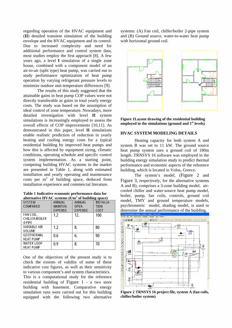
Figure 1Layout drawing of the residential building employed in the simulations (ground and 1st levels) HVAC SYSTEM MODELING DETAILS

Heating capacity for both system A and system B was set to 11 kW. The ground source heat pump system uses a ground coil of 180m length. TRNSYS 16 software was employed in the building energy simulation study to predict thermal performance and economic aspects of the reference building, which is located in Volos, Greece.

The system’s model, (Figure 2 and Figure 3, respectively, for the alternative systems A and B), comprises a 3-zone building model, air-cooled chiller and water-source heat pump model, boiler, pump, fan coils, controls, ground coil model, TMY and ground temperature models, psychrometric model, shading model, is used to determine the annual performance of the building.

Figure 2 TRNSYS 16 project file, system A (fan coils, chiller/boiler system)

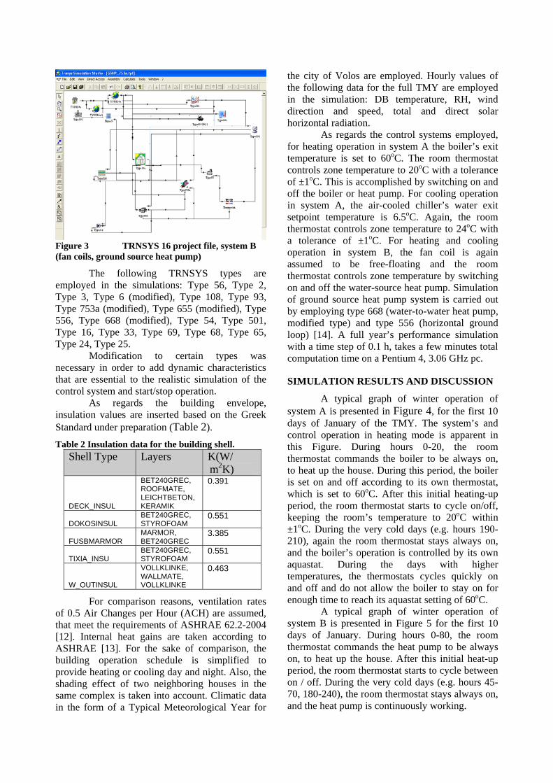
Figure 3 TRNSYS 16 project file, system B (fan coils, ground source heat pump)

The following TRNSYS types are employed in the simulations: Type 56, Type 2, Type 3, Type 6 (modified), Type 108, Type 93, Type 753a (modified), Type 655 (modified), Type 556, Type 668 (modified), Type 54, Type 501, Type 16, Type 33, Type 69, Type 68, Type 65, Type 24, Type 25.

Modification to certain types was necessary in order to add dynamic characteristics that are essential to the realistic simulation of the control system and start/stop operation.

As regards the building envelope, insulation values are inserted based on the Greek Standard under preparation (Table 2).

Table 2 Insulation data for the building shell. Shell Type Layers K(W/

m2K)

DECK_INSUL

BET240GREC, ROOFMATE, LEICHTBETON, KERAMIK

0.391

DOKOSINSUL BET240GREC, STYROFOAM

0.551

FUSBMARMOR MARMOR, BET240GREC

3.385

TIXIA_INSU BET240GREC, STYROFOAM

0.551

W_OUTINSUL

VOLLKLINKE, WALLMATE, VOLLKLINKE

0.463

For comparison reasons, ventilation rates of 0.5 Air Changes per Hour (ACH) are assumed, that meet the requirements of ASHRAE 62.2-2004 [12]. Internal heat gains are taken according to ASHRAE [13]. For the sake of comparison, the building operation schedule is simplified to provide heating or cooling day and night. Also, the shading effect of two neighboring houses in the same complex is taken into account. Climatic data in the form of a Typical Meteorological Year for

the city of Volos are employed. Hourly values of the following data for the full TMY are employed in the simulation: DB temperature, RH, wind direction and speed, total and direct solar horizontal radiation.

As regards the control systems employed, for heating operation in system A the boiler’s exit temperature is set to 60oC. The room thermostat controls zone temperature to 20oC with a tolerance of ±1oC. This is accomplished by switching on and off the boiler or heat pump. For cooling operation in system A, the air-cooled chiller’s water exit setpoint temperature is 6.5oC. Again, the room thermostat controls zone temperature to 24oC with a tolerance of ±1oC. For heating and cooling operation in system B, the fan coil is again assumed to be free-floating and the room thermostat controls zone temperature by switching on and off the water-source heat pump. Simulation of ground source heat pump system is carried out by employing type 668 (water-to-water heat pump, modified type) and type 556 (horizontal ground loop) [14]. A full year’s performance simulation with a time step of 0.1 h, takes a few minutes total computation time on a Pentium 4, 3.06 GHz pc.

SIMULATION RESULTS AND DISCUSSION

A typical graph of winter operation of system A is presented in Figure 4, for the first 10 days of January of the TMY. The system’s and control operation in heating mode is apparent in this Figure. During hours 0-20, the room thermostat commands the boiler to be always on, to heat up the house. During this period, the boiler is set on and off according to its own thermostat, which is set to 60oC. After this initial heating-up period, the room thermostat starts to cycle on/off, keeping the room’s temperature to 20oC within ±1oC. During the very cold days (e.g. hours 190-210), again the room thermostat stays always on, and the boiler’s operation is controlled by its own aquastat. During the days with higher temperatures, the thermostats cycles quickly on and off and do not allow the boiler to stay on for enough time to reach its aquastat setting of 60oC.

A typical graph of winter operation of system B is presented in Figure 5 for the first 10 days of January. During hours 0-80, the room thermostat commands the heat pump to be always on, to heat up the house. After this initial heat-up period, the room thermostat starts to cycle between on / off. During the very cold days (e.g. hours 45-70, 180-240), the room thermostat stays always on, and the heat pump is continuously working.

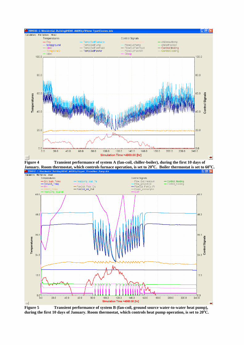
Figure 4 Transient performance of system A (fan-coil, chiller-boiler), during the first 10 days of January. Room thermostat, which controls furnace operation, is set to 20oC. Boiler thermostat is set to 60oC.

Figure 5 Transient performance of system B (fan-coil, ground source water-to-water heat pump), during the first 10 days of January. Room thermostat, which controls heat pump operation, is set to 20oC.

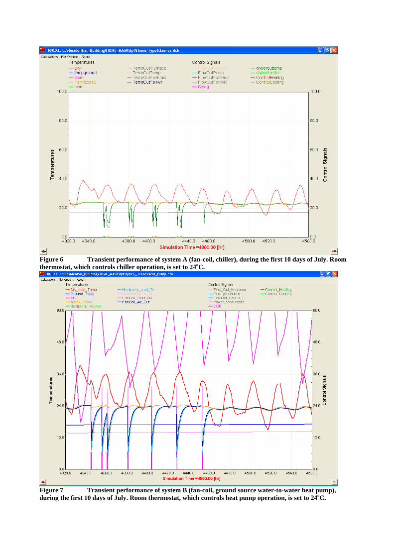
Figure 6 Transient performance of system A (fan-coil, chiller), during the first 10 days of July. Room thermostat, which controls chiller operation, is set to 24oC.

Figure 7 Transient performance of system B (fan-coil, ground source water-to-water heat pump), during the first 10 days of July. Room thermostat, which controls heat pump operation, is set to 24oC.

Figure 8 Yearly performance comparison between systems A (chiller-boiler) and B (ground source heat pump). Figures 4 and 5 reveal much less on/off cycling of the ground source heat pump system.

A typical graph of summer operation of system A is presented in Figure 6, for the first 10 days of July of the Typical Meteorological Year. The system’s and control operation in heating mode is apparent in this Figure. The onset of high ambient temperatures at about 4330 h will require, after a time lag of several hours, the starting of the chiller operation. The chiller stays on during the hot hours of each day, until the ambient temperature levels drop after 4460 h. The small size of the chiller is responsible for the presence of only two on/off cycling during one day (in contrast to the high boiler cycling).

A typical graph of summer operation of system B is presented in Figure 8 for the first 10 days of July of the TMY. The ground source heat pump’s operation in cooling mode is apparent in this Figure. It must be noted that also in the cooling mode the ground source heat pump presents very little on/off cycling (one cycle each day). This presents important advantages in energy consumption as shown in the comparison of yearly performance of the alternative systems in Figure 8. In interpreting this Figure, we should keep in mind that boiler consumption kWh’s are thermal, while chiller and heat pump consumption kWh’s are electrical.

Figure 9 Summary of system A heating performance: effect of thermostat setting (20 versus 22 oC) and boiler size (11 vs 22 kW). EFFECT OF CONTROL SETTINGS AND EQUIPMENT SIZING

The performance summary for the heating season is compared in Figure 9 for the reference system A (11 kW boiler, thermostat set to 20oC), a variation with the room thermostat set to 22oC and another variation with a 22 kW boiler. According to these results, increasing the thermostat setting by 2oC would significantly increase yearly heating energy consumption.

On the other hand, the oversized boiler is predicted to result in a relatively low fuel

consumption penalty. However, the detail of simulation of boiler operation in the specific model is not adequate to assess the full penalty (starting losses of the boiler etc). Good engineering practice results to normal area per cooling unit of about 25-35 m2 per ton (3.6 kW) for commercial buildings in Greece. Lower values correspond to higher ventilation rates (e.g. classrooms, laboratories etc). Higher values are indicative also of residential buildings. However, building HVAC systems designers tend to overdimension the equipment. Apart from the operation expenses, this practice naturally penalizes installation and maintenance cost, and could damage the overall payback time advantage of ground source heat pump. Level II systems simulations, as those demonstrated here, allow exact sizing of the equipment with good estimates of percentage of failure to cover heating and cooling load peaks. EFFECT OF CHILLER COP - CONTROL

A high efficiency chiller is expected to significantly improve system’s performance [15]. Figure 10 presents a map of COP characteristics of the standard air-cooled chiller employed in system A, as function of chilled water temperature level and ambient dry bulb temperature levels.

Figure 10 COP characteristics of standard chiller employed in system A Before considering the adoption of a better chiller, one should check the total electricity consumption for cooling in system A. Before this, we perform a comparative check for two different room thermostat settings: 24 and 26oC respectively. It is interesting to note that no compressor cooling is necessary when the room thermostat is set to 26oC. Even for the extremely

low thermostat setting of 24oC, very low electricity consumption is predicted for system’s A chiller (Figure 11). This could be attributed to the mild climate of Volos, the high degree of insulation of the house and the heavy construction that leads to a high heat capacity [16]. Of course, a chiller with 50% overall increase in COP, compared to the standard chiller of Figure 10, would demonstrated even lower power consumption according to Figure 11. However, there would be no hope for payback of the added cost. Even the necessity of compressor cooling for this house is questionable.

Figure 11 Summary of performance in cooling mode: system A with standard –versus- high efficiency chiller. EFFECT OF HEAT PUMP COP

Comparative computations were carried out to assess the effect of high efficiency heat pumps in system B. Figure 12 presents the COP characteristics of the reference GSHP in heating and cooling mode. We may readily assess the effect of installing a high efficiency heat pump, say with a 50%- higher overall COP in heating mode. Indicative results of this type of computation are presented in Figure 13. Remarkable gains in yearly energy consumption are predicted.

CONCLUDING REMARKS

• Detailed simulation of the building envelope and HVAC equipment, despite its increased complexity, is increasingly applied in building HVAC systems design optimization.

• In this paper, a detailed simulation of the HVAC system operation of a residential building is carried out, which allows good understanding of its transient operation and allow more realistic system’s sizing.

• Level II modelling allows good assessment of the effect of control settings, chiller or heat

pump COP characteristics, equipment sizing, ventilation rates and other design parameters.

• The already reported by others, increased advantage of GSHPs in southern climates, is confirmed in the specific case study, where system’s design optimization was assisted by detailed building energy simulations.

Figure 12 Heating and cooling mode characteristics of the reference ground source heat pump.

Figure 13 Summary of heating performance system B with standard –vs- high efficiency heat pump. • In general, the computations confirm what is

known from experience. Only the fuel consumption penalty of the oversized boiler seems to be underestimated.

• Further development of building systems’ models, despite its complexity, is proven worthwhile in providing more realistic routes of system optimization.

REFERENCES

[1] Directive 2002/91/EC, 16 December 2002 [2] Doing more with less: Green paper on Energy Efficiency (COM(2005) 265 final 22.6. 2005). http:// europa.eu.int/comm/energy/efficiency/index_en.htm [3] Hepbasli, A., Akdemir, O. and E. Hancioglu, Experimental study of a closed loop vertical ground source heat pump system. Energy Conversion and Management 2003, 44 (4) 527–548. [4] Doherty, P.S., Al-Huthaili, S., Riffat, S.B. and N. Abodahab Ground source heat pump––description and preliminary results of the Eco House system. Applied Thermal Engineering 2004, 24: 2627–2641 [5] Sanner, B., Karytsas, C., Mendrinos, D. and L. Rybach Current status of ground source heat pumps and underground thermal energy storage in Europe Geothermics 2003, 32: 579–588 [6] Zogou, O. and A. Stamatelos. Effect of climatic conditions on the performance of heat pump systems for space heating and cooling. Energy Conversion and Management 1998, 39(7):609–622 [7] Sauer H.J. and R.H. Howell Heat Pump Systems. Wiley, New York, 1983. [8] Florides, G.A., Tassou, S.A., Kalogirou, S.A. and L.C.Wrobel, Measures used to lower building energy consumption and their cost effectiveness. Applied Energy 73 (2002) 299–328 [9] LTTE/ University of Thessaly: Exergo-economic Optimization of Air-to-Air Heat Pumps for Space Heating and Cooling. Final Report, “PENED” Program, Volos 1999. Available in Greek at: www.mie.uth.gr/labs/ltte/pubs.htm [10] Sakellari, D. and Per Lundqvist, Energy analysis of a low-temperature heat pump heating system in a single-family house. Int. J. Energy Res. 2004; 28:1-12 [11] Sakellari, Dimitra Modeling the Dynamics of Domestic Low-Temperature Heat Pump Heating Systems for Improved Performance and Thermal Comfort-A Systems Approach. PhD Thesis, Royal Institute of Technology, Stockholm, Sweden 2005. [12] ANSI/ASHRAE Standard 62.2-2004 Ventilation and Acceptable Indoor Air Quality in Low-rise Residential Buildings. [13] ASHRAE Handbook Vol.1, Fundamentals 2005 [14] T.E.S.S. Component Libraries for TRNSYS, version 2.0. User’s Manual, Madison WI 2004. [15] Brodowicz, K. and T. Dyakowski, Heat Pumps. Butterworth-Heinemann 1993. [16] Kalogirou, S.A., Florides, G. and S.Tassou, Energy analysis of buildings employing thermal mass in Cyprus Renewable Energy 27 (2002) 353–368