OPTIMIZATION OF MULTIPURPOSE RESERVOIR …studentsrepo.um.edu.my/8286/1/KHA100096_Mohammad_Heydari.pdf · (1) Saya adalah satu-satunya pengarang/penulis Hasil Kerja ini; (2) Hasil

OPTIMIZATION OF MULTIPURPOSE

RESERVOIR OPERATION USING

EVOLUTIONARY ALGORITHMS

MOHAMMED HEYDARI

FACULTY OF ENGINEERING

UNIVERSITY OF MALAYA

KUALA LUMPUR

2017

OPTIMIZATION OF MULTIPURPOSE RESERVOIR

OPERATION USING EVOLUTIONARY ALGORITHMS

MOHAMMED HEYDARI

THESIS SUBMITTED IN FULFILMENT OF THE

REQUIREMENTS FOR THE DEGREE OF DOCTOR OF

PHILOSOPHY

FACULTY OF ENGINEERING


KUALA LUMPUR

2017

i


ORIGINAL LITERARY WORK DECLARATION

Name of Candidate: Mohammad Heydari (I.C/Passport No: X95385931 )

Registration/Matric No: KHA100096

Name of Degree: PhD

Title of Thesis: Optimization of multipurpose reservoir operation using evolutionary

algorithms

Field of Study: Water Resources Engineering

I do solemnly and sincerely declare that:

(1) I am the sole author/writer of this Work;

(2) This Work is original;

(3) Any use of any work in which copyright exists was done by way of fair dealing

and for permitted purposes and any excerpt or extract from, or reference to or

reproduction of any copyright work has been disclosed expressly and

sufficiently and the title of the Work and its authorship have been

acknowledged in this Work;

(4) I do not have any actual knowledge nor do I ought reasonably to know that the

making of this work constitutes an infringement of any copyright work;

(5) I hereby assign all and every rights in the copyright to this Work to the

University of Malaya (“UM”), who henceforth shall be owner of the copyright

in this Work and that any reproduction or use in any form or by any means

whatsoever is prohibited without the written consent of UM having been first

had and obtained;

(6) I am fully aware that if in the course of making this Work I have infringed any

copyright whether intentionally or otherwise, I may be subject to legal action

or any other action as may be determined by UM.

Candidate’s Signature Date:

Subscribed and solemnly declared before,

Witness’s Signature Date:

Name:

Designation:

Safri

Highlight

ii

UNIVERSITI MALAYA

PERAKUAN KEASLIAN PENULISAN

Nama: Mohammad Heydari (No. K.P/Pasport: X95385931 )

No. Pendaftaran/Matrik: KHA100096

Nama Ijazah:

Pengoptimuman operasi takungan pelbagai guna menggunakan algoritma evolusi

Bidang Penyelidikan: Kejuruteraan Sumber Air

Saya dengan sesungguhnya dan sebenarnya mengaku bahawa:

(1) Saya adalah satu-satunya pengarang/penulis Hasil Kerja ini;

(2) Hasil Kerja ini adalah asli;

(3) Apa-apa penggunaan mana-mana hasil kerja yang mengandungi hakcipta telah

dilakukan secara urusan yang wajar dan bagi maksud yang dibenarkan dan apa-

apa petikan, ekstrak, rujukan atau pengeluaran semula daripada atau kepada

mana-mana hasil kerja yang mengandungi hakcipta telah dinyatakan dengan

sejelasnya dan secukupnya dan satu pengiktirafan tajuk hasil kerja tersebut dan

pengarang/penulisnya telah dilakukan di dalam Hasil Kerja ini;

(4) Saya tidak mempunyai apa-apa pengetahuan sebenar atau patut

semunasabahnya tahu bahawa penghasilan Hasil Kerja ini melanggar suatu

hakcipta hasil kerja yang lain;

(5) Saya dengan ini menyerahkan kesemua dan tiap-tiap hak yang terkandung di

dalam hakcipta Hasil Kerja ini kepada Universiti Malaya (“UM”) yang

seterusnya mula dari sekarang adalah tuan punya kepada hakcipta di dalam

Hasil Kerja ini dan apa-apa pengeluaran semula atau penggunaan dalam apa

jua bentuk atau dengan apa juga cara sekalipun adalah dilarang tanpa terlebih

dahulu mendapat kebenaran bertulis dari UM;

(6) Saya sedar sepenuhnya sekiranya dalam masa penghasilan Hasil Kerja ini saya

telah melanggar suatu hakcipta hasil kerja yang lain sama ada dengan niat atau

sebaliknya, saya boleh dikenakan tindakan undang-undang atau apa-apa

tindakan lain sebagaimana yang diputuskan oleh UM.

Tandatangan Calon Tarikh:

Diperbuat dan sesungguhnya diakui di hadapan,

Tandatangan Saksi Tarikh:

Nama:

Jawatan:

Safri

Highlight

iii

ABSTRACT

Today, the water resources are among the great human treasures. Optimal reservoir

operation, due to the numerous needs, shortcomings and restrictions on the use of these

resources is necessary. The main purpose of this study was presenting a model for an

optimal operation of multi-purpose dams of water resources systems. In this study, a

hybrid evolutionary algorithm model (HPSOGA) and linear programming (LP) has been

developed for optimizing the operation of reservoirs with the objectives of maximizing

hydroelectric power generation, meeting the water demand for agricultural purposes and

predicting the cost and estimating amount of agriculture products.

An improved particle swarm algorithm (HPSOGA) is used to solve complex problems

of water resources optimization. One of the main problems of this method is premature

convergence and to improve this problem, the compound of the particle swarm algorithm

and genetic algorithm were evaluated. The basis of this compound is in such a way that

the advantages of the Particle Swarm Optimization (PSO) algorithm and Genetic

Algorithm (GA) have been applied simultaneously. Two efficient operators of Genetic

Algorithm, that is, mutation and crossover are used in the obtained algorithm, the

mutation causes an increase in the diversity of the population and the intersection of

information between the particles of the population. To evaluate the hybrid algorithm,

optimization of hydro-power energy of Karun dams were considered.

Cases studied in this research were reservoirs of Karun I, Karun III and Karun IV. The

three dams are located in a consecutive series of Karun River in Iran. In order to optimize,

41 years of the common statistical period were used. Then, the optimal output of the

problem in the form of curves that represent the desired amount of discharge from the

reservoir at a specified time interval were prepared and compared with the Lingo model.

The regression analysis and artificial neural networks (ANN) were used to check the

quality of the results.

iv

By using the Weibull distribution, the base year which is consistent with the percent

probability of agricultural needs was determined for downstream of the Karun III dam.

To achieve the best cultivation pattern, initially the arable land was categorized into 6

classes and only 2100 hectares of agricultural irrigable land that had the best agricultural

conditions were studied. The amount of water allocated to the mentioned land was about

6.240 MCM. Seventeen important agricultural products of the region were used for the

modelling. The optimization problem was modelled with the aim of maximizing the

ultimate value of agriculture in terms of the number of acres of each crop. The described

model was resolved by linear programming and evolutionary algorithms in Microsoft

Excel (Solver). The results showed full compliance of these two methods. To estimate

and predict the cost of the different stages of farming, and the cost of fertilizers needed

for agricultural products, the obtained results of cultivation pattern per acre multiplied to

cost breakdown values in tables taken from the ministry of agriculture.

Comparing the results of the combination of the PSO and GA algorithms makes clear

that the obtained algorithm increased flexibility and improving the ability of the PSO

algorithm to create the population with high-speed convergence and it is very applicable

to solve the problems of operation optimization of water resources. To compare the

accuracy of the results, three criteria were used for RMSE, NRMSD and CV. In all the

obtained results, i.e. optimum release, optimum storage and the produced energy, for all

dams, the accuracy of HPSOGA was better than GA and GA accuracy was remarkably

better than PSO. However, exceptionally, the accuracy of the GA algorithm was

approximately 34% better than the HPSOGA algorithm for only the optimal storage

capacity at Karun IV Dam. The overall results show that the optimal values have higher

importance in the preparation of the rule curve, especially in periods of drought.

Keywords: Karun River, Optimization, Hydropower, Optimal Release, Cropping

Pattern

v

ABSTRAK

Pada zaman moden ini, sumber air merupakan salah satu khazanah terpenting bagi

umat manusia. Operasi optima tempat takungan air diperlukan bagi memenuhi pelbagai

keperluan dan sekatan adalah diperlukan bagi mengawal sumber yang terhad ini. Tujuan

utama bagi kajian ini adalah untuk memzahirkan sebuah model bagi satu sistem

empangan pelbagai-fungsi yang beroperasi secara optima bagi satu sistem punca air. Di

dalam kajian ini, satu model “hybrid evolutionary algorithm” (HPSOGA) dan “linear

programme” (LP) telah dibangunkan bagi mencapai satu sistem operasi takungan air yang

optima dengan bermatlamatkan untuk mendapatkan penghasilan kuasa hidroelektirk yang

maksima bagi memenuhi permintaan agrikultur dan juga bagi mendapatkan satu jangkaan

kos serta jumlah produk bagi industri agrikultur tersebut.

Bagi partikel algorithm (HPSOGA) yang telah dikembangkan, ia digunakan sebagai

medium penyelesaian bagi masalah-masalah kompleks berkaitan dengan isu tahap optima

bekalan air. Salah satu permasalahan berkaitan perkara ini adalah tentang isu

penggabungan pra-matang, dan bagi menyelesaikan isu tersebut bahan gabungan bagi

partikel algorithm dan genetiknya perlu dinilai. Asas bagi gabungan ini adalah di dalam

bentuk kebaikan dari Particle Swarm Optimization (PSO) algorithm dan Genetic

Algorithm (GA) yang digunakan secara sekali gus. Dua operator genetik algorithm yang

berkesan dalam mendapatkan algorithm ialah “mutation (mutasi)” dan “crossover

(persilangan)” di mana sistem mutasi akan menyebabkan kenaikan jumlah di dalam

kepelbagaian populasi dan percambahan maklumat antara partikel-partikel populasi

tersebut. Bagi menilai algorithm hibrid tersebut, tahap optima kuasa hidro bagi Empangan

Karun harus dipertimbangkan.

Kajian kes bagi tujuan kajian ini akan difokuskan kepada empangan Karun I, III dan

IV. Ketiga-tiga empangan ini terletak selari dengan Sungai Karun di Iran. Bagi

vi

mendapatkan satu tahap optima, jangka masa statistik selama 41 tahun telah digunakan.

Kemudian, hasil “output” optima bagi masalah tersebut yang dipamerkan di dalam bentuk

lengkungan di mana ia mewakili jumlah yang ingin dilepaskan dari tangkungan tersebut,

pada hentian masa yang spesifik disediakan dan dibandingkan dengan model Lingo.

Dalam menggunakan ‘pengagihan Weibull’, asas tahun yang memiliki konsistensi

selari dengan peratusan keberangkalian keperluan agrikultur telah dikenalpasti bagi

empangan Karun III. Bagi mencapai corak pertanian yang terbaik, pada asasnya tanah

yang terlibat akan dikategorikan kepada enam kelas dan hanya 2100 hektar tanah

agrikulur (Kelas Pertama) yang memiliki keadaan agrikultur terbaik akan dikaji. Jumlah

air yang dibekalkan kepada tanah yang terlibat adalah sebanyak 6.240 MCM. 17 produk

terpenting agrikultur di dalam satu kawasan adalah digunakan sebagai model. Optimasi

permasalahan telah dicorakkan dengan matlamat memaksimakan nilai akhir agrikultur di

dalam bentuk jumlah ekar tanah bagi setiap hasil tanaman. Model yang diterangkan

adalah diselesaikan melalui suatu sistem ‘linear programming’ dan ‘evolutionary

algorithm’ di dalam Microsoft Excel (Solver). Keputusan menunjukkan persetujuan yang

positif di atas kedua-dua kaedah ini. Untuk mendapatkan jangkaan bagi langkah-langkah

penanaman yang terlibat dan kos baja yang diperlukan bagi produk agrikultur, keputusan

berkenaan corak pertanian dalam jumlah ekar yang diperolehi telah didarabkan dengan

kos pecahan jumlah di dalam jadual yang diambil dari kementerian agrikultur.

Dalam membuat perbandingan antara keputusan gabungan PSO dan GA algorithm,

adalah jelas bahawa algorithm yang diperolehi meningkat dari segi fleksibiliti dan juga

meningkatkan kebolehan PSO algorithm dalam mencipta populasi gabungan kadar segera

dan ini sangat membantu dalam menyelesaikan isu berkenaan operasi bekalan air secara

optima. Untuk bandingkan ketepatan keputusan,terdapat tiga krateria yang digunakan

RMSE,NRMSD dan CV. Daripada semua keputusan yang diperolehi, contoh

vii

pembebasan optima, Penyimpanan Optima dan tenaga yang dibebaskan untuk semua

Empangan , ketepatan HPSOGA lebih baik daripada GA dan Ketepatan GA jauh lebih

baik jika dibandingkan dengan PSO. Walaubagaimanapun ketepatan algoritma GA

sangat baik dengan anggaran 34% lebih baik daripada algoritma HPSOGA hanya untuk

kapasiti simpanan optimal di Empangan karun IV. Keputusan keseluruhan menunjukkan

bahawa jumlah optima memiliki kepentingan yang lebih tinggi dalam bentuk persediaan

peraturan lengkungan, terutama di dalam musim kemarau.

Kata kunci: Sungai Karun, Pengoptimalan, Kuasa Hidro, Siaran Optimal, Corak

Tanaman.

viii

ACKNOWLEDGEMENTS

First praise is to Allah, the Almighty, on whom ultimately we depend for sustenance

and guidance, second, I would like to express the deepest appreciation to my supervisor

Assoc. Prof Dr. Faridah Othman, whose expertise, understanding, generous guidance and

support made it possible for me to work on a topic that was of great interest to me. Without

her supervision and constant help, this thesis would not have been possible.

I would like to thank the University of Malaya and Faculty of Engineering for

providing me a great chance to perform my Ph.D.

I would like to express my gratitude to the Ministry of Education (MOE) Malaysia, for

supporting me through the Malaysian International Scholarships (MIS).

In addition, a thank you to Dr. Mohammad Sadegh Sadeghian for finding out time and

for being ever so kind to give his precious advice regarding the topic of my research as

well as data providing.

Finally, and most importantly, I would like to thank my wife Marziyeh. Her support,

encouragement, quiet patience and unwavering love were undeniably the bedrock upon

which the past eight years of my life have been built.

ix

TABLE OF CONTENTS

Abstract ............................................................................................................................ iii

Abstrak .............................................................................................................................. v

Acknowledgements ........................................................................................................ viii

Table of Contents ............................................................................................................. ix

List of Figures ................................................................................................................ xiii

List of Tables................................................................................................................ xviii

List of Symbols and Abbreviations ............................................................................... xxii

List of Appendices ....................................................................................................... xxiv

CHAPTER 1: INTRODUCTION .................................................................................. 1

1.1 Background .............................................................................................................. 1

1.2 Problem statement ................................................................................................... 4

1.3 Significance of the study ......................................................................................... 5

1.4 Objective of Research .............................................................................................. 7

1.5 Scope of the study .................................................................................................... 8

1.6 Thesis outlines ......................................................................................................... 9

CHAPTER 2: LITERATURE REVIEW .................................................................... 11

2.1 Introduction............................................................................................................ 11

2.2 Principles of reservoir operation modelling .......................................................... 14

2.2.1 Governing relations in general reservoir operation problems .................. 14

2.2.2 The general structure of reservoir operation problem .............................. 18

2.2.3 Reservoir operation as a decision-making process ................................... 19

2.3 Methods for solving optimal reservoir operation .................................................. 23

2.3.1 Simulation models .................................................................................... 24

x

2.3.2 Optimization models ................................................................................ 25

2.4 Linear Programming .............................................................................................. 29

2.4.1 LP literature review .................................................................................. 29

2.4.2 Linear programming ................................................................................. 30

2.4.3 Methods for solving linear programming problems ................................. 31

2.4.4 Introducing popular optimization models ................................................ 34

2.5 Evolutionary Optimization Algorithms ................................................................. 37

2.5.1 Overall view of an evolutionary algorithm .............................................. 38

2.5.2 Genetic Algorithm (GA) .......................................................................... 39

2.5.3 Particle Swarm Optimization (PSO) ........................................................ 41

2.6 Principles of Cropping Patterns ............................................................................. 44

2.6.1 Cropping Pattern Definition and Advantages .......................................... 44

2.6.2 Performing Cropping Pattern Consideration ............................................ 45

2.6.3 Previous Studies of Cropping Pattern ...................................................... 46

CHAPTER 3: METHODOLOGY ............................................................................... 49

3.1 Introduction............................................................................................................ 49

3.2 The Study Area ...................................................................................................... 54

3.2.1 Karun and Dez catchment ........................................................................ 54

3.2.2 Flood control in the current situation ....................................................... 56

3.2.3 Hydropower in the current situation ......................................................... 60

3.3 Methods ................................................................................................................. 62

3.3.1 Description of the optimization problem .................................................. 63

3.3.2 The constraints of the problem ................................................................. 66

3.3.3 Data required for the models .................................................................... 72

3.3.4 Description of the flood control ............................................................... 76

3.3.5 Description of the optimal cropping pattern ............................................. 86

xi

3.4 A description of optimization methods................................................................ 100

3.4.1 Genetic Algorithm .................................................................................. 100

3.4.2 Particle swarm optimization algorithm .................................................. 108

3.4.3 HPSOGA ................................................................................................ 111

3.5 A description of computational tools ................................................................... 116

3.5.1 LINGO .................................................................................................... 116

3.5.2 Solver in Excel ....................................................................................... 117

3.6 A description of performance measures .............................................................. 118

3.6.1 RMSE ..................................................................................................... 118

3.6.2 Regression .............................................................................................. 118

3.6.3 Artificial Neural Network ...................................................................... 119

3.6.4 Compared to the wet situation ................................................................ 125

CHAPTER 4: RESULT AND DISCUSSION ........................................................... 126

4.1 Introduction.......................................................................................................... 126

4.2 Hydro power generation ...................................................................................... 131

4.2.1 Calibration test by Linear Programming (LINGO) ................................ 135

4.2.2 Validation test by ANN and Regression ................................................ 139

4.3 Reservoir Storage................................................................................................. 151

4.3.1 Calibration test by Linear Programming (LINGO) ................................ 151

4.3.2 Validation test by compared to the wet situation ................................... 154

4.4 The release rule curves figures ............................................................................ 166

4.5 Optimal Cropping Pattern .................................................................................... 169

4.5.1 Calibration test by Linear Programming (Solver-Excel)........................ 172

4.5.2 Validation test by sensitivity analysis: ................................................... 173

4.6 Accuracy of optimization algorithms (PSO, GA and HPSOGA) ........................ 174

4.6.1 Optimal hydroelectric generation ........................................................... 174

xii

4.6.2 Optimal release ....................................................................................... 177

4.6.3 Optimal storage ...................................................................................... 180

4.7 Predicting the Cost of agricultural products ........................................................ 183

CHAPTER 5: CONCLUSION AND RECOMMENDATION ............................... 186

5.1 Introduction.......................................................................................................... 186

5.2 Conclusion ........................................................................................................... 188

5.2.1 System release rule and reservoir balancing functions........................... 188

5.2.2 Cropping pattern ..................................................................................... 189

5.2.3 Hydropower generation .......................................................................... 192

5.2.4 Flood control .......................................................................................... 193

5.3 Recommendation ................................................................................................. 194

5.3.1 Reservoir rule curves considerations ...................................................... 194

5.3.2 Cropping pattern suggestions ................................................................. 194

5.3.3 Suggestions for hydropower generation modelling ................................ 195

5.3.4 Suggestions for flood control ................................................................. 196

References ..................................................................................................................... 198

List of Publications and Papers Presented .................................................................... 208

Appendix ....................................................................................................................... 213

Appendix A Optimization by HPSOGA method .......................................................... 213

Appendix B Calibration by LINGO (Sample: Karun 4) ............................................... 222

Appendix C Artificial Neural Nework (Matlab Code) ................................................. 223

Appendix D Lingo Codes (Compared to the wet situation) .......................................... 225

Appendix E Genetic Algorithm Code ........................................................................... 232

Appendix F PSO code for three reservoirs ................................................................... 250

Appendix G NSGA II code for three reservoirs............................................................ 255

xiii

LIST OF FIGURES

Figure 2.1: The relationship between two reservoirs in a multi – reservoir system. ..... 15

Figure 2.2: Allocating the capacity of reservoir to different volumes (Faridah Othman,

Sadeghian, Heydari, & Rezaei, 2012) ............................................................................. 18

Figure 2.3: Operational studies of reservoirs (Faridah Othman et al., 2012) ................ 24

Figure 2.4: Schematic representation of optimization process ...................................... 27

Figure 2.5: Steps to solve linear programming problems by using the simplex method

......................................................................................................................................... 32

Figure 2.6: Procedure of an evolutionary algorithm ...................................................... 38

Figure 3.1: Summary of applied methodology in this study .......................................... 53

Figure 3.2: Watershed map for Karun and Dez catchment area .................................... 55

Figure 3.3: Schematic picture of Dez and Karun Reservoirs System and consumption

areas................................................................................................................................. 56

Figure 3.4: Dams and Sub-catchments considered in the flood study ........................... 58

Figure 3.5: Rating curve for Karun IV spillway ............................................................ 59

Figure 3.6: Rating curve for Karun III spillway ............................................................ 59

Figure 3.7: Rating curve for Karun I spillway ............................................................... 59

Figure 3.8: Area-Volume-Elevation relationship for Karun IV reservoir ..................... 60

Figure 3.9: Area-Volume-Elevation relationship for Karun III reservoir ...................... 60

Figure 3.10: Area-Volume-Elevation relationship for Karun I reservoir ...................... 60

Figure 3.11: Schematic view of a multi-reservoir system of Karun .............................. 62

Figure 3.12: Area-Volume-Elevation relationship for Karun IV reservoir ................... 68

Figure 3.13: Area-Volume-Elevation relationship for Karun III reservoir .................... 69

Figure 3.14: Area-Volume-Elevation relationship for Karun I reservoir ...................... 70

Figure 3.15: Reservoir Inflows ...................................................................................... 74

xiv

Figure 3.16: Layout of flood control simulation ............................................................ 80

Figure 3.17: 100 year flood control of Karun IV dam ................................................... 82

Figure 3.18: 100 year flood control of Karun III dam ................................................... 83

Figure 3.19: 100 year flood control of Karun I dam ...................................................... 83

Figure 3.20: 200 year flood control of Karun IV dam ................................................... 84

Figure 3.21: 200 year flood control of Karun III dam ................................................... 84

Figure 3.22: 200 year flood control of Karun I dam ...................................................... 85

Figure 3.23: Relations of flood control storage equivalent for a 100-year flood, the

interval Upper Karun....................................................................................................... 85

Figure 3.24: The relation between flood control reservoir storage in upstream and 100-

year flood in the upper Karun range ............................................................................... 86

Figure 3.25: The flowchart of the cropping pattern and estimating the average cost of

agricultural products methodology ................................................................................. 88

Figure 3.26: The agricultural network ........................................................................... 91

Figure 3.27: Genetic algorithm flowchart .................................................................... 104

Figure 3.28: Non-dominated answers in Pareto range ................................................. 105

Figure 3.29: Genetic algorithm with non-recessive sorting of solutions ..................... 107

Figure 3.30: Particle swarm optimization algorithm flowchart ................................... 111

Figure 3.31: The combination of Particle Swarm Optimization Algorithm and Genetic

Algorithm (Production HPSOGA hybrid model) ......................................................... 115

Figure 3.32: The real neural schematic cell and artificial neural network ................... 121

Figure 3.33: The schematic of ANN model (input and output of our model) ............. 122

Figure 4.1: The obtained results for input, output and storage volume in the Karun I

reservoir (m3) ................................................................................................................ 128

Figure 4.2: The obtained results for input, output and storage volume in the Karun III

reservoir (m3) ................................................................................................................ 129

Figure 4.3: The obtained results for input, output and storage volume in the Karun IV

reservoir (m3) ................................................................................................................ 130

xv

Figure 4.4: Comparison of 4 optimization method's results for the optimal monthly

amount of hydroelectric generation (MW) for Karun I dam......................................... 136


amount of hydroelectric generation (MW) for Karun III dam ...................................... 137


amount of hydroelectric generation (MW) for Karun IV dam ...................................... 138

Figure 4.7: Karun 1 neural network training details .................................................... 139



Figure 4.10: MSE train and test for Karun I ................................................................ 141

Figure 4.11: MSE train and test for Karun III.............................................................. 142

Figure 4.12: MSE train and test for Karun IV ............................................................. 143

Figure 4.13: Q Residual Plot Karun I .......................................................................... 148

Figure 4.14: S Residual Plot Karun I ........................................................................... 148

Figure 4.15: Q Line Fit Plot Karun I ............................................................................ 148

Figure 4.16: S Line Fite Plot Karun I........................................................................... 148

Figure 4.17: Normal Probability Plot Karun I ............................................................. 148

Figure 4.18: Q Residual Plot Karun III ........................................................................ 149

Figure 4.19: S Residual Plot Karun III ........................................................................ 149

Figure 4.20: Q Line Fit Plot Karun III ......................................................................... 149

Figure 4.21: S Line Fite Plot Karun III ........................................................................ 149

Figure 4.22: Normal Probability Plot Karun III ........................................................... 149

Figure 4.23: Q Residual Plot Karun IV ....................................................................... 150

Figure 4.24: S Residual Plot Karun IV ........................................................................ 150

Figure 4.25: Q Line Fit Plot Karun IV ......................................................................... 150

Figure 4.26: S Fite Plot Karun IV ................................................................................ 150

xvi

Figure 4.27: Normal Probability Plot Karun IV .......................................................... 150

Figure 4.28: Results of optimal storage for Karun I reservoir ..................................... 151

Figure 4.29: Results of optimal storage for Karun III reservoir .................................. 152

Figure 4.30: Results of optimal storage for Karun IV reservoir .................................. 153

Figure 4.31: The inflow time series for Karun I, III and IV reservoirs ....................... 156

Figure 4.32: The difference between the inflow and average inflow in Karun I ......... 157

Figure 4.33: The difference between the inflow and average inflow in Karun III ...... 157

Figure 4.34: The difference between the inflow and average inflow in Karun IV ...... 158

Figure 4.35: The difference between the drought and wet situation in Karun 1 dam .. 159

Figure 4.36: The difference between the drought and wet situation in Karun III dam 160

Figure 4.37: The difference between the drought and wet situation in Karun IV dam 161

Figure 4.38: The difference between the average inflow and inflow in during the drought

condition (MCM) for Karun IV .................................................................................... 162

Figure 4.39: Evaporation relationship with the area and volume of reservoir (Loucks,

Stedinger, & Haith, 1981) ............................................................................................. 163

Figure 4.40: Results of optimal release details for Karun I reservoir .......................... 166

Figure 4.41: Results of optimal release details for Karun III reservoir ....................... 167

Figure 4.42: Results of optimal release details for Karun IV reservoir ....................... 168

Figure 4.43: The minimum water required to provide the desired capacity (m3) ........ 171

Figure 4.44: The difference between the minimum amount of agricultural land and the

optimal amount of agricultural land (ha) for each agricultural product. ....................... 172

Figure 4.45: Comparison of the NRMSD & CV errors for the optimization algorithms

(PSO, GA and HPSOGA) which are used to calculate the amount of hydroelectric power

generated in Karun I reservoir....................................................................................... 175



generated in Karun III reservoir .................................................................................... 176

xvii



generated in Karun IV reservoir .................................................................................... 177


(PSO, GA and HPSOGA) which are used to calculate the amount of optimal release in

Karun I reservoir ........................................................................................................... 178



Karun III reservoir......................................................................................................... 179



Karun IV reservoir ........................................................................................................ 180


(PSO, GA and HPSOGA) which are used to calculate the amount of optimal storage in








xviii

LIST OF TABLES

Table 3.1: Relevant features of dams under study ......................................................... 58

Table 3.2: Hydropower characteristics........................................................................... 73

Table 3.3: Evaporation Rate from Open Water surface in (mm per day) at time t ........ 73

Table 3.4: Demand Irrigation (MCM) existing irrigation (partial) ................................ 74

Table 3.5: Downstream capacity of dams based on 100 year return period flood and

designed flood control volume (cms) .............................................................................. 79

Table 3.6: Flood peak discharge of Karun IV river ....................................................... 81

Table 3.7: Flood peak discharge of Karun III river........................................................ 81

Table 3.8: Flood peak discharge of Karun I river .......................................................... 82

Table 3.9: The soil classification in downstream of Karun III (area in hectares) .......... 91

Table 3.10: Input amount of the problem (The data in this table is assumed only for the

case study and annual time distribution is considered) ................................................... 92

Table 3.11: Computed value of problem (The data in this table is assumed only for the

case study and annual time distribution is considered) ................................................... 94

Table 3.12: The average consumed quantity and cost of fertilizer per acre (Currency unit:

TOMAN, Weight: Kg) .................................................................................................... 96

Table 3.13: The average cost of producing one hectare of agricultural products according

to the different stages of farming (Currency unit: Toman) ............................................. 97

Table 4.1: The optimal solution of the objective function by HPSOGA algorithm and

calibration method (LINGO) ........................................................................................ 131

Table 4.2: Percent of the average monthly energy deficit in various reservoirs .......... 131

Table 4.3: Maximum monthly energy shortage in different reservoirs (GWh) ........... 131

Table 4.4: Monthly average values of primary energy production (GWh) .................. 131

Table 4.5: Monthly average values of secondary energy production (GWh) .............. 131

Table 4.6: Monthly average values of total energy production (GWh) ....................... 132

Table 4.7: Average primary plant factor coefficient for study area reservoirs ............ 132

xix

Table 4.8: Average secondary plant factor coefficient for study area reservoirs ......... 132

Table 4.9: Average total plant factor coefficient for study area reservoirs .................. 132

Table 4.10: Monthly average spillage in study area reservoirs (MCM) ...................... 132

Table 4.11: Monthly average of storage in Karun reservoirs (MCM) ......................... 132

Table 4.12: Monthly average of release from turbine in Karun reservoirs (MCM)..... 133

Table 4.13: Monthly Peak Demand as Percentage of Annual Peak Demand .............. 135

Table 4.14: Validation results for hydroelectric power generation .............................. 139

Table 4.15: Summary of MSE results .......................................................................... 144

Table 4.16: Summary of regression statistics output ................................................... 145

Table 4.17: ANOVA results for Karun I ...................................................................... 146

Table 4.18: ANOVA results for Karun III ................................................................... 146

Table 4.19: ANOVA results for Karun IV ................................................................... 146

Table 4.20: Inputs specifications and coefficients of the regression equation for Karun I

....................................................................................................................................... 147

Table 4.21: Inputs specifications and coefficients of the regression equation for Karun

III ................................................................................................................................... 147

Table 4.22: Inputs specifications and coefficients of the regression equation for Karun

IV .................................................................................................................................. 147

Table 4.23: Validation results for optimal reservoir storage ........................................ 154

Table 4.24: Time series of Karun I reservoir inflow .................................................... 154

Table 4.25: Time series of Karun III reservoir inflow ................................................. 154

Table 4.26: Time series of Karun IV reservoir inflow ................................................. 155

Table 4.27: The difference between the average inflow and inflow in during the drought

condition (MCM) for Karun IV .................................................................................... 162

Table 4.28: The details of Karun reservoirs storages ................................................... 163

Table 4.29: The average amount of evaporation in Karun reservoirs in mm............... 164

xx

Table 4.30: The average of Lt value in Karun reservoirs ............................................. 164

Table 4.31: The average of “at” value in Karun reservoirs ........................................... 165

Table 4.32: Validation results for optimal release amount .......................................... 169

Table 4.33: The optimal area of agricultural land for production (hectares) (The data in

this table is calculated only for the problem constraints and conditions) ..................... 169

Table 4.34: The amount of consumed fertilizer in acre in optimum cropping pattern

(Weight unit: Kg) .......................................................................................................... 170

Table 4.35: Solver option for evolutionary algorithm ................................................. 172

Table 4.36: The optimal area of agricultural land for production (hectares) and sensitivity

report of linear programming ........................................................................................ 173

Table 4.37: Comparison of the error of the optimization methods (PSO, GA and

HPSOGA) which are used to calculate the amount of hydroelectric power generated in









HPSOGA) which are used to calculate the amount of optimal release in Karun I reservoir

....................................................................................................................................... 178


HPSOGA) which are used to calculate the amount of optimal release in Karun III

reservoir......................................................................................................................... 179


HPSOGA) which are used to calculate the amount of optimal release in Karun IV

reservoir......................................................................................................................... 180


HPSOGA) which are used to calculate the amount of optimal storage in Karun I reservoir

....................................................................................................................................... 181

xxi


HPSOGA) which are used to calculate the amount of optimal storage in Karun III

reservoir......................................................................................................................... 182


HPSOGA) which are used to calculate the amount of optimal storage in Karun IV

reservoir......................................................................................................................... 183

Table 4.46: The estimated cost of planting, maintenance and harvesting.................... 184

Table 4.47: The cost estimation of consumed fertilizer in acre in optimum cropping

pattern (Currency unit: TOMAN) ................................................................................. 185

xxii

LIST OF SYMBOLS AND ABBREVIATIONS

MILP : Mixed Integer Linear Programming

LP : Linear Programming

DP : Dynamic Programming

BLP : Binary Linear Programming

ILP : Integer Linear Programming

GAMS : General Algebraic Modeling System

AMPL : A Mathematical Programming Language

MINLP : Mixed Integer Nonlinear Programming

BINLP : Boolean integer nonlinear programming

CalSim : The California Simulation of Insurance Markets

OASIS : Operational Analysis and Simulation of Integrated Systems

MCM : Million Cubic Meters

CMS : Cubic Meter per Seconds

M : Meter

M2 : Square meters

M3 : Cubic meters

MCM : Million Cubic Meters

km2 : Square kilometer

Ha : Hectare

TOMAN : A super unit of the official currency of Iran (10 RIALS)

GRG : Generalized Reduced Gradient

FAO : Food and Agriculture Organization

MWN : The minimum required water (m3 per hectare)

APH : Average production per hectare (ton)

xxiii

PVT : The product value per tonne (TOMAN)

MT : The minimum tonnage (ton)

MAL : Maximum available agricultural land (ha)

VPH : Value per hectare (10 Rials/ Toman)

MLN : The minimum land required for production (ha)

MWND : Minimum water required to provide the desired capacity (m3)

TAW : The total allocated water (MCM)

OPT : The optimal area of agricultural land for production (ha)

K 1 : Karun I

K 3 : Karun III

K 4 : Karun IV

MOL : Maximum operation level

UG : Upper Gotvand dam

RMSE : Root Mean Square Error

NRMSD : Normalized Root Mean Square Deviation

CV : Coefficient of Variation

xxiv

LIST OF APPENDICES

Appendix A: Optimization by HPSOGA method ………………………...…... 226

Appendix B: Calibration by LINGO (Karun 4)………………………….…….. 235

Appendix C: Artificial Neural Network (Matlab Code)……………..………… 236

Appendix D: Lingo Codes (Compared to the wet situation)…………………… 238

Appendix E: Genetic Algorithm Code……………………………………….… 245

Appendix F: PSO code for three reservoirs…………………..………………… 263

Appendix G: NSGA II code for three reservoirs………………………..……… 268

1

CHAPTER 1: INTRODUCTION

1.1 Background

Water is the most important requirement for all living creatures after oxygen. Life and

health of all beings including human, plants and animals, depends on water. Although 75

percent of Planet Earth is composed of water, only one percent is the usable fresh water.

This insignificant amount is not spread on the earth uniformly. This limitation is one of

the most significant challenges in countries with arid and semi-arid regions.

Variability of rainfall regimes and discrepancies in the discharge regime of the river

with water needs and river flow in different years make it necessary to build storage

systems to regulate the natural flow of rivers. One way to deal with the problems in water

resources management and lack of appropriate temporal and spatial distribution, is the

optimal use of reservoirs. Dams are designed and constructed in order to resolve such

problems. Providing water for municipal, agricultural and industrial consumption is one

of the main purposes for reservoir operation and planning. Moreover, because of water

needs in the region, sometimes storage system includes a reservoir, and sometimes several

in a row on the river or a network of reservoirs on the river and its tributaries are designed.

Surface reservoirs play an important role to reduce the damage caused by lack of water

in the dry months or years by regulating river flow and water delivery from wet months

to the dry months and also in some cases by regulating beyond the year.

Irrigation: In most countries, agricultural purposes have the highest water level

consumption. Water stored in the reservoir has increased monthly and annual rate of

discharge and subsequently irrigated acreage and gross income will be risen. On the other

hand, water resource development costs have increased at a considerable rate and so any

attempt at optimizing of the required reservoir volume due to the economic aspects of the

plan will be a step forward on the path of economic development. Therefore, optimal

2

operation and management of water resources, among giving proper response to the needs

of this part, leads to reduced wastage of water and increases the level of production yield

and gains sustaining development in agriculture.

Flood control: Flood control is another aims of constructing dams. Not only dams are

known as main source in providing water, they also create high capacity for developing

tourism industry.

Tourism: In most countries in the world, dams and their reservoirs are considered as

the most important tourist attraction and attract numerous tourists annually.

Hydropower generation: One of the aims of constructing dams is hydroelectric energy.

Nowadays, the hydropower and thermal energies have the highest share in producing the

world electricity. Although, problems and limitations of producing electricity in thermal

power sources due to technical issues, the imperatives of environmental criteria, resources

constrains have caused that, by the time the general trend in the world of power

generation, hydroelectric plants will be more preferred. The potential energy of water

behind a dam, provide hydroelectric energy. In this case, energy of water depends on

stored water of the dam and height difference between the water source and the

withdrawal of water from the dam.

The next issue is the optimal operation of the reservoir, considering the objectives like

drinking water needs, industrial, agricultural, hydroelectric purposes, flood control,

tourism, etc. Variety of purposes of water resources management makes decision making

complex and difficult. One of the principles of water resource management is

implementation and correct operation of the dam reservoirs.

Efficient approaches and appropriate solutions must be considered for operating

reservoirs as one of the most important components of water resources management.

3

Application of such approaches leads to create balance between available limited

resources and high demand, optimization of water use in agriculture, municipal and

industry and finally sustainable development in water resources management. Nowadays,

water management and water protection are highly important in developing and

developed countries. In order to system enhancement and equitable management of water

resources, complaint to the prescribed principles and technical planning is necessary.

Using practical planning techniques to optimize water resources, due to their simplicity

and applicability are very important.

Application of optimization techniques to exploit the reservoirs is the main issue in the

management and planning of water resources and, it has been highly considered by

researchers in the past two decades.

Optimization techniques have been significant during the last few decades in

management and operation of complex system reservoirs. Overall, management of the

reservoir consists of two stages, Simulation and optimization processes.

In arid and semi-arid regions like most parts of Iran, water is the substantial limiting

factor in agricultural development. Therefore, the essential issue in resolving the

challenges in water management is maintaining a balance between supply and demand.

According to the fact that the economic value of water is directly related to the crop

cultivation pattern and their density and that this pattern undergoes many changes over

the utilization years, by investigating these changes in all areas of the country the current

water status in terms of pattern and density should be compared with the proposed status.

Agricultural activities are the main indicators of development in countries like Iran.

Whenever the allocation of resources is in non-optimal state at the level of producers and

enterprises, one cannot expect the resources to be efficiently allocated at the macro level.

In agriculture, it is very complicated to find an optimal cropping pattern with the aim of

4

obtaining the maximum net profit by considering the constraints such as water resources,

soil, regional needs, cost, etc. It is impossible to ensure that whether the proposed

cropping pattern offers the maximum profitability by using common methods such as trial

and error, because practically infinite number of cropping patterns should be tested.

Mathematical programming is used for agricultural programming and determining the

optimal crops cultivating pattern in an agricultural unit or in a certain region. The aim of

linear programming is to maximize or minimize the objective function of the farm’s

manager regarding some of the constraints (available resources) and decision variables

(activities) simultaneously.

1.2 Problem statement

Storage systems often lack the appropriate and academic utilization patterns in Iran.

Therefore, investigating the methods and providing suitable models for the optimal

utilization of such systems during normal operation and periods of intense drought had

high priority. On the other hand, the limitation on the total amount of water and the fixed

total amount of it, in contrast to increasing industrialization process and the subsequent

process of increasing urban growth in demand in various fields, creates a set of factors

related to each other and brings the issue of water crisis to the fore in the near future. So,

efficient management and operation of the facilities have special importance.

Optimal operation of reservoirs requires management of storage to predict the output

current for the future input current. Optimization is a fundamental concept to enhance the

management and optimization of interactive efficiency of dam construction projects. One

of the main priorities for water supply schemes is the appropriate operation of storage

reservoirs. Moreover, codification of operation policy from constructed reservoirs is

socially and economically important. Optimal design of storage reservoirs requires the

regulation of operation based on the determination of the reservoir input and output values

5

and determination of the relationship between them. Useful volume or reservoir storage

capacity and output control for picking the accurate amount are calculated based on the

indicators of storage system operation. Control the water output of a reservoir at any depth

of water, is done by using a guide, tables and graphs. The tables and charts are used as

operating instructions for the use of water in normal and stressful conditions, proper

maintenance of water levels, operation at the time of the flood and partnership with other

reservoirs.

There are different methods for the operation and storage of water in reservoir. All

these methods determines the amount of current release at the specified time based on a

simple storage system and release for a specified period, the analysis of measured data,

and operation methods. In most reservoirs in the world, rule curve as the main pattern of

operation, determine the amount of storage and release of water in storage reservoirs.

A rule curve describes how much storage reservoir at different times of the year should

be in the reservoir so that the amount of needed water can always be supplied.

The study is going to answer the following questions:

1. How efficient is the rule curve of Karun dams for supplying required water by the

purpose of minimizing the failure of supply?

2. How is the performance of the existing rule curve system in comparison with

mathematical programming techniques such as linear programming?

1.3 Significance of the study

Iran is located in the arid and semi-arid region. Many areas of the country do not have

enough water for agricultural activities so water is the main factor in most of the

agricultural areas. Iran is located in the Middle East including 5% of the world population,

6

just have access to only one percent of the world water. Average annual rainfall in Iran is

246 millimeters that means a quarter of the world average rainfall (Sadeghi,

Moatamednia, & Behzadfar, 2011).

The total amount of rainfall in Iran is about 400 billion cubic meters. About 310 billion

cubic meters (over 77%) rains in the mountainous areas and only 90 billion cubic meters

rains on the plains ("Water Resources and Quality in Iran," 21/12/2016). About 286

billion cubic meters will be lost by evapotranspiration and approximately 114 billion

cubic meters will remain in a year. Obviously, by the population increasing to 100 million

in 1400, Iran will be in water deficit conditions. Non-uniform rainfall distribution in space

and time are also the main problems in the water sector. So using the potential capacity

and the hydro potential of the wet areas in order to supply water needs in arid areas is

inevitable. To produce 65 million tons of agricultural products, about 85 billion cubic

meters of water will be consumed. Even if there are enough agricultural land, but water

resources of the country will not let the production increase enough, in accordance with

the population growth.

Lack of enough water resources in Iran has been recognized as one of the key

challenges in the water sector, with an increase in water demand due to the expansion of

agricultural, industrial and urban activities. These challenges have been intensified.

The socioeconomic development of the regional society in the Karun River Basin, the

case study, depends on the optimum development and management of the available water

resources in the region. The river system is coming under increasing pressure to satisfy

the demands of domestic, industrial, agricultural, environmental, navigation and

hydroelectric power generation users, whilst at the same time maintain an adequate flow

in the river systems both in terms of quantity and in terms of quality.

7

The hydraulic performance of the Karun and Dez Rivers demonstrate significant flood

damaging potential to the adjacent fields and population, especially in the south reaches

downstream of Ahwaz city. Short duration and high discharges are the characteristics of

winter floods.

The fast development of multipurpose dams in the Karun and Dez rivers is placing

additional pressure on the current operational dams and structures. The developed and

under construction schemes are in significant need of management tools to be established

to assist planning, evaluation, controlling and operating reservoirs in the system and to

size the flood control and conservation storage requirements for each scheme.

Without immediate actions to be taken to manage and control the water resources of

the river system, the combination of abstraction and flood events will inevitably lead to

further water shortage and contaminated water quality, which will impact further on all

water users and waterside residents.

This study has two innovations for optimizing the reservoir operation:

Planning for present and future using regression analysis and artificial neural

networks (in situations of data insufficiency or data generation for the future)

Integrated and optimal resource management, from planning to operation.

(Connecting the optimizer model to optimal water allocation for agricultural

land and estimate the amount of agricultural products and predict the cost

before implementation.

1.4 Objective of Research

The main objectives of this study are as follows:

8

1. Maximize the hydroelectric power generation in Karun dams (or minimize

shortage of hydro power supply)

2. Optimize water supply (Determine the optimal release of the dam for domestic,

agricultural and industrial purposes)

3. Minimize shortage of agricultural water supply (Identify the optimal cropping

patterns for downstream of Karun 3 dam )

4. Predict costs and quantities of agricultural products in the obtained optimal

cropping pattern

In other words, the main purpose of the study was to achieve an optimal operation

program of the water system consisting of Karun I, Karun III, and Karun IV dams for the

determined purpose in the operation.

1.5 Scope of the study

For the following five reasons, the study area was considered in the Karun Basin:

1. The problem should include more than two reservoirs in series.

2. Reservoirs must meet the objectives of producing a hydroelectric power plant, water

supply and providing downstream agricultural needs.

3. Agricultural information at downstream of reservoirs should be accessible.

4. All dams should have long input data (at least 30 years)

5. The data must be accurate and complete.

The purpose of this study is to examine the “maximum potential” scenario, taking into

account the requirements of water for industrial and domestic demand, for irrigation and

9

hydropower. It is assumed that raw data (such as soil surveys and land maps showing

irrigable potential) will be available.

The principal work activities of this component are as follows:

1. Collect all required hydro-meteorological data;

2. Collect data on existing reservoirs;

3. Review all main potential developments for hydropower, water supply and

irrigation.

1.6 Thesis outlines

The first chapter briefly discussed some generalities about the problem and different

methods of solving the problem, and the importance and purpose of the study.

Chapter 2 presents a review of related literature about different methods of optimizing

operation of reservoirs. Chapter 2 consists of four sections. The first section contains

generalities about optimal reservoir operation problems and then discusses about

optimization process and methods. In the second part, a statistical overview of the

published papers in field of optimal reservoir operation is presented. In the third part, a

linear programming method and its related literature in details are discussed. In the fourth

part, a complete description of new optimization algorithms, including background of

research, process optimization, and advantages and disadvantages of each methods have

been presented.

The third chapter, explains the whole study area, and after that the methods and tools

used in the study (Lingo for linear programming and Genetic Algorithm and Particle

Swarm Optimization and HPSOGA as a hybrid model consisting of these two methods

for evolutionary algorithms).

10

In the fourth chapter, the results and discussions obtained from linear programming

and HPSOGA algorithms and existing conditions are discussed.

Chapter five consists of overall conclusion of the study and suggestions.

11

CHAPTER 2: LITERATURE REVIEW

2.1 Introduction

A multi-objective task, which involves water supply, flood control, energy generation,

and environmental concerns, is called reservoir operation. In order to achieve almost all

goals and most ideal possible performance of the reservoir, we need to analyze and

operates the system optimally by considering the variations in inflow and demands.

Decisions need to be made about releases and storage volumes over a period of time. The

truth is none of the algorithms are capable of satisfying all these aspects of reservoir

operation issues. Mathematical programming and Evolutionary algorithms are very

famous as optimization methods, which have used to solve the optimal reservoir operation

so far. Thus, researchers focus on optimization of reservoir operation more than ever.

Researchers have applied several mathematical programming techniques, such as

Linear Programming (LP) (Needham, Watkins, Lund, & Nanda, 2000), Dynamic

Programming (DP) (C. Cheng, Wang, Chau, & Wu, 2014; Hall, Butcher, & Esogbue,

1968; Li, Wei, Li, Wang, & Yeh, 2014; Zhao, Zhao, & Yang, 2012),and Stochastic

Dynamic Programming (SDP) (P. Liu, Zhao, Li, & Shen, 2012; Saadat & Asghari, 2017;

Shokri, Haddad, & Mariño, 2012; Stedinger, Sule, & Loucks, 1984) to solve different

kinds of reservoir-operation problems optimally. During the last decades, A number of

approximate algorithms are developed, which are trying to combine basic principles of

evolutionary methods to find a method for efficient search in feasible regions.

Evolutionary algorithms (EAs) like Genetic Algorithm (GA) (Ahmed & Sarma, 2005)

(Ashofteh, Haddad, & Loáiciga, 2015; Fallah-Mehdipour, Haddad, & Mariño, 2012;

Ngoc, Hiramatsu, & Harada, 2014), Differential Evolution (Reddy & Kumar, 2007;

Schardong & Simonovic, 2015), Ant Colony Optimization (ACO) (A. Dariane & Moradi,

2010; Kumar & Reddy, 2006; Moeini & Afshar, 2013),, Simulated Annealing (SA)

(Teegavarapu & Simonovic, 2002), Particle Swarm Optimization (PSO) (A.M. Baltar &

12

D.G. Fontane, 2008) (Fallah-Mehdipour, Haddad, & Mariño, 2011; Ostadrahimi, Mariño,

& Afshar, 2012; Rahimi, Qaderi, & Abasiyan, 2013), A Hybrid Cellular Automat-

Harmony Search Approach (M. Afshar, Azizipour, Oghbaeea, & Kim, 2017), and

Artificial Neural Networks (ANN) (Wei & Hsu, 2008) are some samples of these methods

(F. Othman, Sadeghian, & Heydari, 2012). A comprehensive survey of these methods can

be found in (W. Yeh, 1985), (Labadie, 2004), (Wurbs, 1993) and (M. H. Afshar &

Shahidi, 2009). It is extensively recognized that there is no single algorithm available to

resolve all reservoir-operation problems, since every problem has its own distinctive

physical and operational typicality’(W. W. G. Yeh, 1985).

Evolutionary methods are suitable for solving nonlinear optimization problems with

large number of complicated variable decisions. The main advantage of these techniques

is achieving a global optimum instead of local optimum. Usually, they are not trapped in

local optima.

In summary, it can be said that various researchers have tried to optimize the operation

of reservoirs using different methods or tools. However, the following two points are

considered less than others:

1- Not paying attention to integrated management

2. Failure of the model for cases where data is not complete or there is no data at all

(like modeling for future)

In this chapter the general principles of reservoir operation modelling has been

introduced then linear programming (LP) and evolutionary algorithms (EA) are discussed

thoroughly.

13

In section related to evolutionary optimization algorithms, the algorithms have been

introduced briefly alongside the optimization process, previous research and strengths

and weaknesses of each algorithm. Then multi objective optimization techniques have

been introduced and after that the general principles, the optimal cropping pattern

application and studies done in this field were discussed. In the end the statistical review

of the published papers on the operation of the reservoir is given.

14

2.2 Principles of reservoir operation modelling

2.2.1 Governing relations in general reservoir operation problems

Governing relations in a multi-reservoir system which are going to be presented in

following paragraphs are general and they are common in both deterministic and dynamic

stochastic models.

Continuity equation:

In fact, Continuity equation is one of the physics laws available in the system and is

based on the rule of Conservation of Mass (Equation 2.1):

𝑆𝑙,𝑡+1𝑥 = 𝑆𝑘𝑡

𝑥 + 𝑞𝑡𝑥 − 𝑟𝑘𝑙𝑡

𝑥 − 𝑒𝑣𝑎𝑘𝑙𝑡𝑥 + ∑𝑑𝑡

𝑥𝑥′

(2.1)

Which Sl,t+1x is the volume of water in the reservoir x at the end of the period, evaklt

x

is the evaporation from mean level of the reservoir, and rkltx is outcome belongs to

reservoir x in t period. ∑dtxx′

is sum of flows which transfer from upstream reservoirs x’

to reservoir x. qtx intermediate inflow into the reservoir upstream region in period t. in the

reservoirs which have no other reservoirs upstream, qtx is as the only flow into the

reservoir but in downstream reservoir, qtx is equal to total interway flows, it means that

discharge from the sub-region is between considered reservoir and upstream reservoir.

Furthermore, it is possible to enter return flows to the system in the format of this

parameter. Figure 2.1 shows a simple two-reservoir system with signs.

15

Figure 2.1: The relationship between two reservoirs in a multi – reservoir system.

Capacity limits:

Reservoir storage in each period should be within the active storage range (Equation

(2.2) :

𝑆𝑚𝑖𝑛,𝑡𝑥 ≤ 𝑆𝑘𝑡

𝑥 ≤ 𝑆𝑚𝑎𝑥,𝑡𝑥 (2.2)

Minimum capacity storage of the system in normal situation is equal to dead storage

(a volume which is designed for sediments) but if reservoir is being used for producing

electric-water energy or entertainment, it is necessary to consider more minimum capacity

storage and the balance of the reservoir shouldn’t be less than a specific level. In this case,

the minimum storage volume of the reservoir would be more than dead storage.

Each reservoir has a fixed maximum capacity that would be indicate by K, at each time

interval, the present volume cannot exceed the amount of capacity (Equation (2.3) :

St ≤ K (2.3)

Figure 2.2 shows different parts of a storage reservoir.

16

Reservoir outflow limitation:

It is possible to have limitations in each period for outflow from each reservoir

Equation (2.4) :

𝑅𝑚𝑖𝑛,𝑡𝑥 ≤ 𝑅𝑘𝑙𝑡

𝑥 ≤ 𝑅𝑚𝑎𝑥,𝑡𝑥 (2.4)

The minimum outflow of the reservoir is considered for cases such as certain needed

discharge, minimum flow to protect environment and aquatic, and boating in multi

reservoir systems. In addition, maximum output of the reservoir may be in the direction

of turbines, rivers, downstream installments capacities and so on.

Evaporation calculation

In every reservoir operational program, the amount of loss from the reservoir as a result

of evaporation should be considered. Usually, infiltration is unlike evaporation,

negligible. Values of evaporation and rainfall related to the lake of the dam are expressed

based on height, which according to the level of lake, their volumes are determined for

the reservoir. For this purpose, first, a simple linear regression is generated between

storage and reservoir level and then, its volume of the reservoir in each period is

calculated based on pure evaporation height. Mean storage level based on the beginning

and end of the period storage, is calculated by following Equation (2.5) :

𝐴𝑘𝑡𝑥 = 𝑎1

𝑥 + 𝑎2𝑥 ( 𝑆𝑘𝑡

𝑥 + 𝑆𝑘𝑙𝑡𝑥 )/2 (2.5)

Where Aktx is mean reservoir x level in t period and corresponds to storage volume at

the beginning of t period Sktx , and storage volume at the end of t period or beginning of

t+1 period, is Skltx . a1

x and a2x Are regression coefficients.

Evaporation volume from reservoir level during the t period equals to Equation (2.6) :

17

𝑒𝑣𝑎𝑘𝑙𝑡𝑥 = 𝐴𝑘𝑡

𝑥 ∗ ( 𝑒𝑣𝑎𝑝𝑡𝑥 − 𝑟𝑎𝑖𝑛𝑡

𝑥) (2.6)

Where evakltx , is the evaporation volume from surface of reservoir x in the t period. In

this equation, resultant of evaporation and rainfall are incorporated into the formula so

evakltx can be negative and it means in that period, rainfall was more than evaporation.

Equations described above are the most important, essential and basic equations,

relationships to model any reservoir at any desired time interval. The primary objective

of every reservoir is to supply water to downstream over the time and space. The other

objectives may include reservoir volume management for recreational purposes, flood

control and the release of water management for the production of hydroelectric energy.

Reservoirs have been constructed to change the natural flow of rivers. Reservoir

capacity and release policy defines the extent so that surface flow of water can be stored

until it will be released in future. Using of reservoirs for the temporary storage often leads

to complete loss of water because of evaporation and residual, reservoirs bring changes

in regional climate, area and the river system. They also may cause displacement of

people and their habitats. The benefits of building a new reservoir include water supply

of downstream, hydro power production, navigation, recreation, and etc., the benefits

obtained from the reservoirs may be significant, but the cost should also not be forgotten.

Comparison between benefit and cost is always a challenge because it is difficult to

express them in a standard mode.

A storage volume of the reservoir is divided into three major and main usages:

• Active Storage, which is used to supply the water of downstream regularly,

recreational development in the area, hydropower, etc.

• Dead Storage, which is needed to collect the required sediment

18

• Flood storage, which is preserved in the reservoir to prevent damage downstream

during flood

These three storages are demonstrated in Figure 2.2, separately. Distribution of flood

storage capacity and active storage may have changed over the year. For instance, it is

not essential to consider flood capacity in certain months of the year that have no

experience of flooding.

Figure 2.2: Allocating the capacity of reservoir to different volumes (Faridah Othman,

Sadeghian, Heydari, & Rezaei, 2012)

These entire capacities can often be modelled separately and then added together to

determine the total capacity.

2.2.2 The general structure of reservoir operation problem

The general structure of a base model that constitutes the base of most of optimization

models for the operation of reservoirs is as follows:

Min Z: ∑ loss t ( Rt , Dt , St) (2.7)

Subject to:

19

St+1=St - It – Rt – Et – It (t=1, 2... n) (2.8)

Stmin≤ St≤ Cap (t=1, 2... n) (2.9)

0≤Rt≤Rmaxt (t=1, 2... n) (2.10)

St, Et, Lt, Rt≥0 (2.11)

Where: (Equations above), Z: objective function, Loss t: the cost of operation in month

t, which depends on the outlet need and the reservoir storage capacity in month t, Rt:

release from reservoir in month t, Dt: water demand in month t, St: the storage capacity

of reservoir in month t, N: number of intervals for programming, Smin: minimum volume

water storage in reservoir, Cap: total volume capacity of water in reservoir, Rmaxt:

maximum release from reservoir in the duration of t, Et: amount of evaporation from

reservoir in month t, Lt: amount of water leaking from reservoir in month t and It: amount

of inflow into the reservoir in month t. (Karamouz, Szidarovszky, & Zahraie, 2003).

In the objective function of this model, the total loss in the operation period is

minimized. Different types of loss functions have been proposed for the optimization of

reservoir operation models which are mostly based on a function of water deficit to meet

the demand and the difference between the current storage and the design storage of water

of the reservoir in every month. The loss of failing to meet the demands is calculated by

comparing the total released water with the total needs of the system.

2.2.3 Reservoir operation as a decision-making process

The storage capacity needed to fulfill a given set of purposes depends on the policy

used to operate the reservoirs. Given the major capital investments needed to build a

reservoir, the environmental and social impacts of reservoirs, there is a strong incentive

to find efficient operating policies that minimize the storage needed to satisfy the water

needs and maximize the benefits provided by existing reservoirs. This pressure has

increased in recent years due to a greater environmental and social awareness and to the

restricted financial conditions that most nations are enduring. Proposals to construct new

20

reservoirs to meet the always increasing water and energy demands and to reluctant

politicians and an averse society. Water resource managers are thus being forced to

review the operating policies of existing reservoir systems to find ways to further improve

their performance.

Estimating reservoir-operating policies that maximize benefits provided by the

operation of reservoirs and minimize their adverse impacts is not an easy task. Operating

reservoirs is a complex decision-making process that involves a large number of

variables, considerable risk and uncertainty, and often multiple conflicting objectives.

Reservoirs may be built to satisfy a single purpose, but multipurpose reservoirs are often

preferable because of the increased benefits derived from them.

In addition, the reservoir construction and operational costs can be distributed over a

number of activities. While some of the reservoir purposes may be fairly compatible, like

low flow augmentation for navigation and for pollution dilution, others may not be

entirely compatible. For example, for power generation the reservoir should be as full as

possible to increase the head, whereas for flood protection the reservoir should be empty

to provide for maximum storage of floodwaters. In this case, no objective can be fully

satisfied and a balance between them must be achieved.

Reservoirs are often integrated into systems of reservoirs and other control structures.

If operated in a coordinated way, the reservoirs can provide larger benefits than the sum

of the benefits yielded by the independent operation of each reservoir. This is especially

true if the hydrological regime varies widely throughout the system and if the reservoir

system is supposed to satisfy a number of different purposes. Water demands may be met

from other sources thus saving thus saving water stored in the system reservoirs. Also,

the operational benefits can be maximized by selecting the most appropriate set of

reservoirs to satisfy each system objectives. For example, high-head reservoirs can be

21

used to produce energy while reservoirs with high evaporation rates can be used for flood

protection and low-head reservoirs can be used to satisfy water supply demands. As the

size of the system increases, the operation becomes very difficult because of the large

number of variables to be handled. System operators have to coordinate all the water

demands with the water availability, and find the most efficient way to satisfy, all system

objectives, if possible. They have to pay attention to all legal contracts, agreements and

traditions that establish the priorities for the water use. Often, these priorities are not well

established and are subject to dispute. This situation becomes even more complex if the

reservoir system crosses administrative or international borders. Finally, all the

operational decisions have to be made under the uncertainty of future hydrological

conditions. System operators must continually evaluate the trade-offs between short and

long-term uses of water without knowing with certainty the future availability of water.

They may manage reservoir storage space to reduce the risk of flooding, knowing that a

greater emphasis on flood protection may reduce their ability to satisfy for water or energy

demands.

Given the typical scale of reservoir operation problems and the interdependence of all

the factors involved, enormous benefits can be obtained from the reservoir if the correct

operating policy is implemented for successful application of optimization models. One

possible use of optimization models is in real-time operation of reservoir systems. In this

situation, an optimization model is run at each decision time to determine the best

operating decisions. These decisions are computed by solving a multi-period stochastic

optimization problem that maximizes the expected future operational benefits subject to

all operating constraints. However, despite the undeniable potential of this approach and

the amount of research done by the academic community, these types of optimization

models still play a minor role in determining reservoir releases. The following reasons

may explain this lack of success.

22

Agreements on water resources management are difficult to achieve. The interests of

each water user are often incompatible. Each user defends its position with vigor and only

yields his rights with great reluctance. Long and intense negotiations are usually needed

before a consensus is reached, and often the disputes have to be settled by the judicial

system. The agreements or court decisions are usually stated as fixed rules that can be

understood by all interested parties. If an optimization model is to be used to support real-

time reservoir operations, all the interested parties have to accept the model and its results.

This means that all have to accept each one of the mathematical equations that constitute

the model, and agree on which technique should be used to solve the optimization

problem. Since this discussion requires some technical and scientific knowledge, that

some of the individuals involved in the decision process may not have, it may be very

difficult to achieve an agreement. Some individuals may even refuse consensus.

Furthermore, the mathematical programming techniques available to solve

optimization problems are only applicable if the size of the problem is not excessive, or

if all the mathematical equations that constitute the model satisfy some specific set of

conditions. These conditions require simplifications and approximations that prevent a

detailed description of all the physical, hydrological and institutional characteristics of a

reservoir system, as well as of all the needs and objectives of the various water users. If

these simplifications are so severe that the optimization model does not capture the

important characteristics of the reservoir system, the model results are not useful for real-

time operation..

23

2.3 Methods for solving optimal reservoir operation

Operation of reservoirs is one of the most important and complicated issues in usage

of dams that the designers have had challenges with for a long time. One of the most

important solutions is choosing the best study method as well as utilizing the best

engineering techniques. By using these methods and techniques, not only the operational

method is studied, but also the capacity of reservoir is estimated. The most important

methods in determining the capacity of reservoir are: critical period method (mass curve,

sequent peak method, working table), optimization methods or system engineering

techniques (linear programming, dynamic programming) and simulation methods.

Optimization is a method that should result in the best answer to a problem based on given

purpose and limitations defined as mathematical functions. In this method, the design

parameters such as the height of the dam could be estimated using mathematical models.

The general trend of the reservoir studies is depicted in Figure 2.3. As it can be seen

in this figure, having defined the possible options and calculated the reservoir function,

the capacity of the reservoir and type of operation should also be defined.

24

Figure 2.3: Operational studies of reservoirs (Faridah Othman et al., 2012)

2.3.1 Simulation models

Simulation model should predict the reaction of the system relative to a specific policy

as if already the behavior of the system relative to different scenarios is determined (W.

W. G. Yeh, 1985).

Rea

din

g t

he

bas

e dat

a D

efin

ing t

he

capac

ity p

f re

serv

oir

and

met

hod

of

oper

atio

n

Res

ult

of

stu

die

s on r

eser

voir

oper

atio

n

Cal

cula

tio

n o

f re

serv

oir

funct

ion

P

rep

arin

g r

ule

cu

rve

Reservoirs operational studies

Topographic

maps and

surface,

volume, height

Hydrological

data, (yield,

sediment, flood)

Aerologic data

(evaporation,

precipitation)

Water demand

(drinking,

agriculture…)

Design data Economic data

Definition of possible options

Choosing the

computational

method

Optimization

methods

Screening the

options

Simulation method

Choosing the best options (final for the justification

Physical characteristics

(of the reservoir)

The main parameters of

the reservoir

Annual function of the

reservoir

Calculating the function of reservoir using the base data

Evaluating the result of calculation of reservoir function to prepare the rule

curves

Reporting the studies of operation of

reservoirs

Selecting the

calculation methods

Using optimization

methods

Using simulation

method

Power operating

rule curve

Flood control

diagram

Rule curves for

meeting the

demands

Rule curves of

multipurpose

reservoirs

25

Input data for each simulation model can be divided into three parts: constant data,

design data, and raw input flows. Constant data are system parameters, which physical

and economical characteristics and relationships of them are defined and are not variable

just like design parameters. Design data are in fact decision variables, which are

determined during modelling process such as reservoir capacities and power plants. Input

flow is also given to the system as artificial statistics or historical data (Jacoby & Loucks,

1972).

Simulation models can provide system efficiency and performance in different

mixtures of reservoirs, power plants, values of storage volume, desired outputs, etc. and

in this way have a good flexibility. Thus to choose the best mixture of them there is no

good and effective tool. The reason is clear. Each time for a specific state of possible

mixtures, simulation model shows the option by an operation policy and effectiveness.

Now, if it is necessary to check many options, there should be necessary modifications

for each option. This task is impossible in large systems, which have so many options.

Jacoby and Loucks (1972) studied this subject in Delaware area in the USA. This study

consisted of 35 reservoirs, which only 6 reservoirs had determined capacity and the

capacity of the rest of the reservoirs should be determined optimally. Regardless of

variables related to operational policies, needed water and electric – water power plant

and just 2 storage capacity options for each reservoir, the number of generated states

would be 229 and if using of simulation is assumed, the number of simulations should be

equal to that number. In this case, with 1 minute for each execution, more than 10 years

is needed to perform all the possibilities.

2.3.2 Optimization models

As mentioned earlier, simulation models usually cannot obtain the best option. On the

other hand, optimization models can produce the best possible mixture through assuming

26

a special goal such as maximize revenue or minimize damage besides describing a

physical and real phenomenon by logical mathematical equations. Also, due to some

imposed assumptions in the computer program, in optimization models the resulted

answer is not necessarily real optimal, but it is much closer to the real outcome which

justifies the application of optimization for this purpose. Thus, it should be noted that in

addition to these optimization models, there are more limitations, which make some

difficulties in the application of them. Some of these problems may be due to limitations

existing in the solutions. Thus, with all these problems, unique characteristics of

optimization models, has made their application in water resources and particularly the

planning and operation of reservoirs, very attractive. Today, the target of studies scientists

and researchers in water resources management has focused on toward this direction.

Using applied mathematics, they try to solve above-mentioned problems. The number of

articles, which are published in magazines and journals, supports this idea.

Many studies that have been done on the optimization show that it is not possible to

use a general method to solve all the problems of water resources.

Optimization Process

The optimization process of this study is presented in Figure 2.4, and it consists of

seven vital steps.

27

Figure 2.4: Schematic representation of optimization process

1. The first step in this process is expanding a clear understanding of the problem

with a detailed view of the real world. To this end, a number of primitive solutions to

achieve objectives must be defined that consider different aspects of the problem. Also,

some doubts should be in the minds of decision makers as to which opinion to achieve

the goal is the best.

2. Problem definition phase is a phase in which a precise and clear statement of the

problem based on observations must be made and be gained in identification phase and

transparency step of the problem. The mentioned problem definition should define

purpose, the influence of the initial solutions, assumptions, barriers, limitations and

possible available information on sources and markers involved in the problem.

Experience shows that the erroneous definition of the problem leads to failure of analysis.

3. When we define the problem, the next step is developing a mathematical model.

The mathematical model is the mathematical performance of the system or real problem

and is able to perform different aspects of the problem in interpretable form. At first, it

may be that qualitative model structure itself, including unofficial descriptive approach.

From this unofficial qualitative model, an official model may develop. (Part 3 contains

some applied models in order to optimize reservoir operations of dams.)

1) A detailed view

2) Problem definition

3) Developing mathematical model

4) Finding solution for the model

5) Sensitivity analysis phase

6) Validation

7) Performing the solution

28

4. After formulating and developing the model, it is turn to find a solution for the

model. Usually the optimal solution for the model with evaluation outcome sequence is

found. This sequence of operation starts from a primitive solution that is as input of the

model and the generation of the developed solution as output. The developed output is

resubmitted as a new input and the process is repeated under the certain circumstances.

5. Another important phase of this study is a sensitivity analysis phase. Performing

the sensitivity analysis allows us to determine the necessary accuracy of input data and

understanding the decision variables that have the highest influence on the solution. The

sensitivity analysis allows the analyst to see how sensitive the preferred option of

changing assumptions and data is. In sensitivity analysis, analyst modifies the

suppositions or data to enhance the considered option and convert it into optimal choice.

Amount of measured default modification is determining the power of the model.

6. A solution should be tested. Often the solution is tested in a short or long term.

The proposed solution must be validated against the actual performance observation

while the test is being made, and it should be independent of how an optimal solution is

obtained.

7. The final phase is performing the solution. This is the step of using optimal outputs

for decision-making process. Usually, analyst converts his mathematical findings as a

series of understandable and applicable decisions. It may be necessary to train decision-

makers to help them apply the findings to attain the required changes from the current

situation to the desired situation. In addition, they need to be supported until they learn

the mechanism of maintenance and upgrading the solution.

29

2.4 Linear Programming

In order to solve optimal reservoir operation problem, researchers are trying to use

some techniques in relation with programming and management for a long time. Most of

practical and applied problems can be modeled as a linear programming problem

regarding all intrinsic complexities. The mentioned reason and presence of different

solving software of linear programming problems have caused that linear programming

to be used as one of the most practical methods in the field of dam operation for years. In

this research, we introduce optimal operation problems of reservoirs by using linear

programming techniques and discuss about them. Also, objective and multi objective

models were introduced by using some questions. Finally, some popular methods in the

field of modeling such problems are introduced.

2.4.1 LP literature review

Charles Revelle in 1969 decided to act for design and reservoir management by linear

programming and using the Linear Decision Rule (LDR). In this linear decision making

method, reservoir outflow in whole operation period was calculated as the difference

between the storage of the reservoir at the beginning of the period and decision parameter

by solving linear programming (Revelle, Joeres, & Kirby, 1969). In 1970, Loucks applied

the linear model with its probable limitation and its deterministic equivalent for solving

the system of reservoirs (Loucks, 1970)

Cai and his collaborators in 2001, used genetic algorithm with linear programming in

complex problems of water reservoir. The gained results have been reported very

satisfactory (Cai, McKinney, & Lasdon, 2001). in 2005, Reis et al. used combination of

Genetic Algorithm (GA) and Linear Programming (LP) method designed and solved

planning and decision-making for reservoirs of water systems (Reis, Walters, Savic, &

Chaudhry, 2005). In 2006, Reise and his associates performed a combination method

using genetic algorithm (GA) and linear programming (LP) in order to achieve

30

operational decisions for a system reservoir that is applied during optimization term. This

method identifies a part of decision variables named Cost Reducing Factors (CRFs) by

Genetic Algorithm (GA) and operational variables by Linear Programming (LP) (Reis,

Bessler, Walters, & Savic, 2006).

2.4.2 Linear programming

Classical optimization models are linear, nonlinear or dynamic models. Optimization

problems are often divided into linear and nonlinear models. This division is due to the

variable relations. It means that if the relation among all variables is linear, then the

problem is called linear, otherwise it is called nonlinear. Due to the simplicity of linear

programming structure, and applicability of these models as a primitive appropriate

model in water resources management systems, the possibility of solving problem with

large number of variables, with no need for assumptions and primary values, researchers

tend to use this kind of programming in their researches. Another advantage of

mathematical programming are different solutions (like simplex method, interior point

method), the possibility of converting nonlinear problem to linear one, and the possibility

of instant calculation of the final optimal solution.

Maximize c1x1+c2x2+… +cnxn (2.12)

Subject to

x1, x2,…, xn≥0 (2.13)

a11x1+a12x2+… +a1nxn≤b1 (2.14)

a21x1+a22x2+… +a2nxn≤b2 (2.15)

am1x1+am2x2+… +amnxn≤bm (2.16)

In such cases, the objective function is minimized. In the last formulation, we assume

maximization, as minimization problems can be rewritten into maximization problems by

multiplying the objective function by –1.

31

The best method for solving constrained optimization model depends on the specified

mathematical form of the objective function and equations. There is not any

comprehensive method for efficient solving of all the optimization models.

Thus, every mathematical programming model in its best way is only an approximate

description of the actual water resources system. The obtained answer is only optimized

to the prepared model but not to the real problem.

2.4.3 Methods for solving linear programming problems

Essentially, there are two popular methods for a LP model. These models are Simplex

method and its variants and Interior point method (Robere, 2012). These two methods

describe practicable solution term, which can be defined as a confined space with

constraints and variable bounds. Then the optimal point (best method for solution) of the

solution space is found.

Main objective of the graphical method shows acceptable solutions and research

limitations. The method has practical value in solving small problems with two decision

variables and only few constrains (Turban & Meredith, 1994).

Simplex is an algebraic method. The flowchart in Figure 2.5 demonstrates the solution

steps briefly. Details of the simplex can be found in operations research concepts and

cases (Hillier & Lieberman, 2005).

32

Figure 2.5: Steps to solve linear programming problems by using the simplex method

The interior point method is particularly efficient for solving large- scale problems.

For small LP models, the interior point algorithm requires a relatively wide computing,

then after repetition may only an approximation of the optimal solution be obtained. In

contrast, the simplex method requires only a few instant repetitions to find optimal

solution. For large LP models, the interior point method is very efficient, but it provides

33

only one approximate solution. The comparison between these two methods have been

discussed thoroughly in a study by Illés, T. and T. Terlaky (Illés & Terlaky, 2002).

In solving large-scale linear programming problems, we often encounter specially

structured coefficient matrices. The most common structure is as follows:

(2.17)

Where are Ai,j ( 0 ≤ i ≤ k , 1 ≤ j ≤ k ) given matrices. When applying the simplex

method in such cases, we can take advantage of the special structure, and in each simplex

step (moving to a neighboring vertex) we are able to preserve this special structure.

Another special method is the decomposition technique, where the optimal solution of

the large problem can be formulated by using a sequence of the solutions of much smaller

problems, the sizes of each are determined by the sizes of the blocks Ai, (i = 1, 2, …, k).

The most popular decomposition technique is the Dantzig–Wolf method, a discussion of

which can be found in almost all texts of optimization. The classical text of Dantzig

(1963) is a good source for further reading (Dantzig, 1963; Dantzig & Cottle, 1963;

Wolfe, 1963)

If the objective function and one or more constraints are nonlinear, then the problem

becomes one of nonlinear programming. In the case of only two variables, they can be

solved by the graphical approach; however, the feasible decision space may not have

vertices, and even if it does, the optimal solution might not be a vertex. In such cases, the

curves of the objective function with different values have to be compared. This

procedure is shown next.

34

2.4.4 Introducing popular optimization models

Nowadays, many optimization models of operation research, including linear model,

nonlinear model and integer model can be easily analyzed by using computer software.

Among them, some software like GAMS ،GINO ،LINDO ،LINGO ،QSB and TORA can

be mentioned. There are many commercial software packages in the market to solve the

mathematical models. The solving software package is generally a solver engine, which

contains one or more algorithms for solving a specific class or a number of different levels

of mathematical models, like simplex and interior point algorithm for solving LP model.

Below is a brief introduction to some of the most popular models.

EXCEL SOLVER: Excel solver is a powerful tool for optimization problems. This

solver can solve most of optimization problems like linear, nonlinear and integer

programming. This tool was first created by Frontline Systems, Inc (Fylstra, Lasdon,

Watson, & Waren, 1998). Excel solver uses Generalized Reduced Gradient (GRG2)

algorithm in order to optimize nonlinear problems and also uses simplex algorithm for

solving linear programming (Del Castillo, Montgomery, & McCarville, 1996; Kemmer

& Keller, 2010).

LINDO: LINDO performs a robust solution for linear, nonlinear (convex and non -

convex), quadratic, limited degree and integer optimization of probabilities. Demo

version can solve models with 300 variables and 150 constrains (including 30 integer

numbers) (LINDO Systems, 2013).

LINGO: LINGO is considered as a simple and also robust tool for solving linear and

nonlinear programming (Xie & Xue, 2005). One of the major advantages of this tool is

formulizing big problems briefly and analyzes problems. LINDO and LINGO software

were designed by LINDO Systems, Inc. Company in order to solve optimization problems

in university, industry and business. The mentioned products come with books operation

research: applications and algorithms (1994) (Winston & Goldberg, 1994) and an

35

introduction to mathematical programming: applications and algorithms (2003) written

by professor Winston (Winston, Venkataramanan, & Goldberg, 2003). After GAMS,

LINGO is the most robust software of operation research. Among the advantages of

LINGO in comparison with LINDO or GAMS is its power in modeling problems that are

modeled by LINDO, without the need to specify the type of model by the user. While,

LINDO and GAMS don`t have such capability. Another important capability of LINGO

is having a very robust, simple and complete Help. LINGO is a comprehensive language

in order to facilitate all optimization models. Another specification of this software is

having different mathematical functions, statistics and probability, ability to read data

from files and other worksheets and high ability in analyzing model.

GAMS: General Algebraic Modeling System (GAMS) model is a professional

software in solving mathematical optimization problems (Brooke, Kendrick, Meeraus,

Raman, & Rasenthal, 1998). This software has a program for modeling with high

capability in order to obtain optimal value of variables in objective function of a

programming problem. GAMS is used for solving problems like linear programming

(LP), nonlinear programming (NLP) and multiple integer programming (MIP) and

multiple integer linear programming (MINLP) etc. One important specification of GAMS

is that writing its model is independent from the solution. Therefore, we can solve the

model with different methods (linear, nonlinear and integer) by only making changes in

SOLVER. Interpreting the model of mathematical language to GAMS language is often

transparent because GAMS use common English words.

MATLAB: MATLAB programming is undoubtedly one of the most robust computing

programs in the field of mathematics, engineering and technology. There are many

methods for solving linear programming problems. Among them, the simplex method has

specific importance and efficiency for solving problems with average size. There are also

some ways for solving large problems (equations with many variables). All the mentioned

36

methods are in optimization toolbox of MATLAB and these features are used to solve,

linear programming problems. We can simply write the specific functions and programs

by using codes and functions of MATLAB. If the number is high, we can make a toolbox

with them by assigning a subtype. In fact, MATLAB is a simple programming language

with very developed characteristics. Also, this software is easier to use than the other

computer languages (Venkataraman, 2009).

MPL: (Mathematical programming language), product of Maximal Software

company, is a modeling system that allows developers to model efficient optimization

formulation. MPL is able to solve problems with millions of variables and constrains.

MPL works with optimization engines like CPLEX and XPRESS and many other robust

industrial solvers. Trial versions are just used up to 300 constrains for a limited time.

Win QSB: (Quantitative Systems for Business) is a Windows-based decision-making

tool. Win QSB is an educational tool that includes a number of modules that almost covers

all basic methods of operation research and management science. The size of optimization

problems can be worked with Win QSB is almost similar to LINGO and Solver or any

other trial version. The model is flexible in almost any field and can analyze all models

and parameters. The control chart of this software, in addition to charting, gives users

other tools such as Pareto analysis charts, histograms, graph and efficiency of the process,

analysis of data distribution and the corresponding computations.

37

2.5 Evolutionary Optimization Algorithms

Operation of the reservoir is one of the key issues among different water resources

issues. An operation policy includes a set of laws which determines the amount of water

that must be stored or released under different conditions of operation (Wurbs, 1993).

Determining a proper utilization plan of water resources systems, in a way that a good

performance would be gained from the system in all conditions, is called optimization.

As a result, application of optimization method is required in order to determine the

operation schedule of the reservoirs. Optimal Management of dam reservoirs can be very

complex in the real world. Increasing complexity in engineering issues and having a

systematic view to the management, particularly in water resources engineering reduced

efficiency of classic methods. In recent decades, massive efforts have been done in order

to develop and introduce algorithms that are more appropriate.

Meta heuristic algorithms are one of these methods, which have been used

recently in many scientific studies. One difference between Meta heuristic algorithms and

classic algorithm is to provide the set of answers at each step (Meta heuristic algorithms)

instead of producing an Answer (classic methods). In this case, if the problem has only

one optimal answer, it is expected that all answers of Meta heuristic algorithm will be

congruent. Since many problems of water engineering only need good answers and

somehow close to the optimal solution, therefore, the heuristic algorithms that guarantee

such answers were considered.

Evolutionary algorithms are techniques that are based on random searches and are

inspired by natural biological evolution. These algorithms work on the possible solutions

that have superior characteristics. Evolutionary algorithms have no need for other

knowledge and there is no restriction in defining the objective function. These algorithms

are based on populations rather than individuals working for a single solution. Hence, the

search can be done in parallel with each of the individuals. In the case of several optimal

38

solutions (Pareto front) evolutionary algorithms are inherently efficient. Aforementioned

reasons, range of applicability, ease of use and ability to achieve a global optimum

solution make these algorithms the best among methods of solving complex optimization

problems.

In almost all evolutionary algorithms, first a set of randomly generated solutions and

a merit function is calculated, compared and ranked. Then the individuals with the best

solution are chosen to improve the population in next step by mimicking natural processes

such as mating, mutation and foraging. This is done until some of the individuals reach

the optimum and the termination conditions are met (Figure 2.6).

2.5.1 Overall view of an evolutionary algorithm

Creation of a random population

Comparison and ranking between solutions

Creating a new generation inspired by nature, e.g. mutation or crossover.

Repeating stage two of the process.

Figure 2.6: Procedure of an evolutionary algorithm

evaluation

ranking

selectioncrossover

mutation

39

2.5.2 Genetic Algorithm (GA)

Using meta-heuristic algorithms became prevalent when first Genetic Algorithm was

introduced by Golderg in 1989 (Goldberg, 1990). Genetic algorithm is one of heuristic

algorithm that is considered in the field of water resources. East and Hall in 1994 (Esat &

Hall, 1994) used this algorithm to model the four-reservoir system and discussed the high

capability of this algorithm in modeling water resources systems. Another research,

loucks and Oliveira in 1997 (Oliveira & Loucks, 1997), showed the ability of Genetic

Algorithm in dealing with multi-objective reservoir systems. Wardlaw and Sharif also

used a genetic algorithm to optimize a four-reservoir system, and showed that this method

can provide valid and acceptable answers (Wardlaw & Sharif, 1999). A year later, this

work was improved by Sharif and Wardlaw (Sharif & Wardlaw, 2000). Also, for a system

of 10 reservoirs genetic algorithm was used which was designed by Murray and Yakowitz

and were used by Vardla and Sharif. Accuracy of results of genetic algorithm for this

problem is very acceptable (Murray & Yakowitz, 1979). In addition, Cai et al used a

combination of genetic algorithm and linear programming in their study to solve

nonlinear models of water management (Cai et al., 2001). Yuan et al also used a Genetic

Algorithm as a method of combination with the chaotic optimization method and called

it Hybrid Chaotic Genetic Algorithm. This method is used for finding optimal schedule

of a hydroelectric system with consecutive power plants on the horizon 24-hours with

intervals of one hour (Yuan, Yuan, & Zhang, 2002). Chang et al used Genetic Algorithm

to find the rule curve of monthly optimization in a multi-objective of the single dam

system in Taiwan (F.-J. Chang, Chen, & Chang, 2005).

In 2005, Ahmad and Sarma (Ahmed & Sarma, 2005) compared the results of Genetic

algorithm and stochastic dynamic programming in optimizing multi-objective reservoir

system and suggested that this algorithm gives more acceptable results in obtaining

operation policies in reservoir systems.

40

Jian-Xia al in 2005 (Jian-Xia, Qiang, & Yi-Min, 2005), compared the binary-coded

and real-coded Genetic Algorithms and found that real-coded Genetic algorithm results

more earlier and reliable. This research also evaluated the algorithm components such as

selection, crossover and mutation and suggests the best way of ordering them. In 2008,

Cheng et al (C.-T. Cheng, Wang, Xu, & Chau, 2008) compounded the chaos algorithm

and genetic algorithm to introduce a novel Chaos Genetic Algorithm CGA and applied it

for the monthly operation of a hydropower reservoir. They concluded that this method

results better in benchmark optimization problems.

Dariane and Momtahen applied linear operation policy and linear plot by doing

reform bars in the genetic algorithm operators in the multi-reservoir systems(A. B.

Dariane & Momtahen, 2009).

Wang et al in 2011 (Wang, Chang, & Chang, 2011) proposed a Multi-tier Interactive

Genetic Algorithm to deal with large-scale systems with high dimensional variables in

which the system is decomposed to small sub-systems and the optimal solution is found

using the interaction of these sub-systems.

Considering several objectives together as approaching the problems, researchers

tried to improve metaheuristic algorithms to be able to derive trade-offs between

objectives. This led to advent of Multi-Objective Evolutionary Algorithm (MOEAs).

Some proposed EAs by researchers are Non-dominated Sorting Genetic Algorithm

(NSGA) (Srinivas & Deb, 1994), Niched Pareto Genetic Algorithm (NPGA) (Horn,

Nafpliotis, & Goldberg, 1994) that has received good recognition. Cieniawski et al in

1995 (Cieniawski, Eheart, & Ranjithan, 1995) used Genetic Algorithm in a multipurpose

problem of locating a network of groundwater monitoring wells and finally tried to obtain

trade-off curves. They showed that GAs are able to find a large portion of Pareto Frontier

but not all. Deb et al in 2002 (Deb, Pratap, Agarwal, & Meyarivan, 2002) introduced non-

dominated sorting-based multi-objective algorithm which was called non-dominated

41

sorting genetic algorithm II (NSGA-II), which was tested through benchmark problems

and showed much better performance in deriving Pareto Frontiers. Schardong et al in

2012 (Schardong, Simonovic, & Vasan, 2012) used Multi-objective Differential

Evolution to achieve optimal operation of a multipurpose multi-reservoir system and

compared it with the results of NSGA-II. The objectives included minimization of

demand shortage, maximization of water quality and minimization of pumping cost.

2.5.3 Particle Swarm Optimization (PSO)

Particle Swarm Optimization is one of the population-based random search algorithm,

presented for the first time by Kennedy and Eberhart (Kennedy & Eberhart, 1997).

Particle Swarm Optimization algorithm (Eberhart & Shi, 1998, 2001) is based on the

simulation of the movements of birds and fish in a swarm behavior. Like other

evolutionary techniques, this algorithm consists of a population of potential solutions,

which tries to explore the search space. The main difference between this method and

other methods is that each particle has a velocity vector, which helps the particle to change

the direction and improve its position in entire search space.

Kumar and Reddy used proposed particle swarm algorithm as elitism mutation of

influx particles to solve the famous problem of Larson four reservoirs. Then, they

compared results of different methods with those of this method and reported that this

method has many advantages over all other methods tested. (Nagesh Kumar & Janga

Reddy, 2007).

In recent years, several single-objective water systems have been modeled using

Particle Swarm Optimization algorithm. For example, Montalvo et al in 2008 (Montalvo,

Izquierdo, Pérez, & Tung, 2008) used this algorithm in two cases: water distribution

network and water supply tunnel system in New York. Their objective was to compare

the previous results with the ones obtained by PSO. Shourian et al used the combination

of particle swarm algorithm and MODSIM for the design and operation of the Sirvan

42

reservoir system (Shourian, Mousavi, & Tahershamsi, 2008). Cheng et al in 2009 (C.-t.

Cheng, Liao, Tang, & Zhao, 2009) compared DP and PSO algorithm applied in obtaining

sample load curve of hydropower plant. Results showed that PSO is applicable in such

problems.

In recent years, several reforms have been applied to PSO algorithm. Most of these

changes have improved the applicability of the algorithm and some other has caused PSO

to act better in some specific sort of problems. For example FPSO (Fuzzy PSO) and

binary PSO, which was introduced by Kennedy and Eberhart in 1997 (Kennedy &

Eberhart, 1997). In binary variation, every particle represents its position in binary values

which are 0 or 1. In Fuzzy PSO algorithm velocity vector is presented in fuzzy mode (H.

Liu, Abraham, & Zhang, 2007; Shi & Eberhart, 2001).

Zhang et al used combination of article swarm and genetic algorithms to optimize

energy in a multi-reservoir system (Zhang, Wu, Cheng, & Zhang, 2011). In 2013 Afshar

(M. Afshar, 2013) proposed a constrained version of PSO in three variations called

Partially Constrained PSO one (PCPSO1), Partially Constrained PSO two (PCPSO2) and

Fully Constrained PSO (FCPSO). It showed that PCPSO1 might violate the feasible

search area. Therefore, PCPSO2 is introduced by a modification of the storage volume

bounds to remove the flaws of first algorithm and hence enhanced to FCPSO version of

the PSO. Results obtained from two benchmark problems were compared with other

algorithms and showed the superiority of proposed version.

In most cases in which there are several objectives to handle with simultaneously,

MOPSO can be used to deal with such problems. In 2007 Reddy and Kumar (Nagesh

Kumar & Janga Reddy, 2007) studied on elitist-mutated particle swarm optimization

(EMPSO) technique to obtain operation policies applied in multipurpose reservoir

system. They used elitist-mutation technique to improve the performance of standard

43

PSO. At the end they discussed that EMPSO yields better solution compared to Genetic

Algorithm with less function evaluation. In 2007 these researchers also (Reddy & Nagesh

Kumar, 2007) offered EM-MOPSO which they discussed that it gives more efficient

results and good convergence in reaching a true Pareto Front. To facilitate its application

in reservoir problem they used a decision-making approach and showed its competency

in obtaining results.

In 2008 Baltar and Fontane (Alexandre M Baltar & Darrell G Fontane, 2008) used

MOPSO (Multi-Objective Particle Swarm Optimization) to solve a multipurpose

problem. It was applied to a problem of four objectives. They concluded that PSO resulted

in very encouraging results compared to other evolutionary algorithms. In 2011

Ostadrahimi et al (Ostadrahimi et al., 2012) employed a new approach called MSPSO

(Multi-Swarm Particle Swarm Optimization) accompanying HEC-ResPRM simulation

model to estimate the parameters of the rule curves in a multi-reservoir system. In this

research the simulation model evaluates the objective function for each set of the

population made through a new mechanism named multi-swarm PSO algorithm.

44

2.6 Principles of Cropping Patterns

2.6.1 Cropping Pattern Definition and Advantages

The optimal use of natural and human resources is an important economic and social

objectives that in this case, fundamental and sweeping changes in the structure of

agriculture, the extensive involvement of staff and favorable management factors of

production, are necessary to develop the agricultural sector in the country. In this

communication, design and adjust the cropping pattern to determine the amount of

cultivated area and the right combination of products, is utmost important and should be

done in such a way that in addition to the optimal use of existing capacities and access,

regional and national needs are considered.

There are many definitions for cropping pattern, which it seems the most

comprehensive definition is: “cropping pattern refers to determining an agriculture

system with an economic advantage based on state macro politics, local knowledge of

farmers and optimal operation of regional potential observing ecological principles of

products along with preserving the environment.” In addition, cultivation combination

means “The proportion of dedicating fields of an area to various agricultural and garden

products.”

The definition shows that in many regions of the state, growing agricultural and

horticultural crops or operation of fields and forests suits regional potential. Climatic

restrictions, negative balance sheet of valleys water and the need of production stability

make us to move in a way to improve underground water and increase water consumption

efficiency.

In fact, the most important finding of crops pattern and cultivation combinations can

be outlined as follows.

• Improving water efficiency coefficient for agriculture products and scientific use

and optimal operation from other production institutions.

45

• Modifying operation system of natural resources and controlling instability

factors of these resources and effort for maintenance and development.

• Promoting efficiency and paying attention to economics, security and political

values of water in its acquisition, presentation, maintenance and consumption.

• Increasing water acquisition rate, minimizing natural and unnatural water wastes.

2.6.2 Performing Cropping Pattern Consideration

• Performing appropriate cropping pattern guarantees food security and production

stability.

• Performing appropriate cropping pattern is necessary for protecting basic

resources and increasing efficiency production factors.

• Performing appropriate cropping pattern requires coordination and cooperation of

power ministries, agriculture and commercial institutions.

• Accessing stable production in agriculture is in lieu of appropriate operation and

efficiency of basic resources.

• We can guarantee production stability and food security with performing

appropriate cropping pattern.

• We should consume water along with the optimal cropping pattern.

• Paying attention to state climatic conditions, guarantees performing appropriate

cropping pattern and production stability.

• With collecting required rules and terms, basis of performing appropriate

cropping pattern is provided.

• Performing appropriate cropping pattern requires common intrinsic county

planning.

• Performing optimal cropping pattern causes to preserve natural resources.

• With performing an optimal cropping pattern, we reduce adverse effects of

drought.

46

2.6.3 Previous Studies of Cropping Pattern

The complexity of water resource problems leads to increase the application of

systems analysis approaches. Optimization makes it possible to model a process

mathematically along with its constraints. After that, the model could be optimized

utilizing optimization techniques.

Aside from the optimum cropping pattern, the policy makers, employers and

managers in the agricultural sector are very interested to be informed about the amount

of agricultural inputs (such as fertilizers) before the agricultural activities commence.

This knowledge helps them to know the funding requirements as well as storing,

maintaining and managing the agricultural process.

Most of the resources, restrictions, aims and sensitivities of these kinds of matter that

can be compiled with developing models based on linear programming are considered

and determined an optimal cropping pattern. Here are examples of some studies that have

been conducted on determining an optimal cropping pattern especially with the help of

computer software and programming models. Bayat (1999) determined the optimum

cultivation pattern in terms of integrative use of surface and groundwater resources in

Borazjan plain. The results showed that the programming efficiency of implementing the

optimum pattern will be increased respectively 33% and 21% for utilizations of 6 and less

than 6 hectares and utilizations of more than 6 hectares compared to their current pattern.

Also, several studies were done in and outside of Iran by using the application of

mathematical programming techniques in relation to the present study, which are briefly

referred to some of them. Matanga and Mariño (1979) have done a test in which irrigation

programming was with respect to the agricultural pattern and with the help of dynamic

linear programming. These researchers aimed to maximize gross interest for different

products, with respect to water availability limitations in different periods, system

capacity, task force and other possible resources. Lamers and Bruentrup (1996) estimated

47

the economic profitability of five options on fodder crops in West Africa by using linear

programming. Based on these results, the proposed model includes a set of options in

which, the economic benefit is at the highest level possible. The results show that the use

of forage for livestock feed has the most profitable and the burning forage is involved

minimum benefit for farmers. Omoregie and Thomson (2001) have studied the

competition in oilseeds production using linear programming method in Nigeria. In their

study, oilseed production is limited by the constraints of land and oil extraction plants.

They concluded that the Middle Belt region is the most economical area in grain

production than other areas because of its central location, and it has the highest shadow

value per hectare. On the contrary, the West has the least shadow price per hectare of

land. The results of this study are concerned that transportation costs as the main factor

in reducing the profitability of oilseed production. D. Singh, Jaiswal, Reddy, Singh, and

Bhandarkar (2001) used linear programming to optimize cropping pattern in Pakistan.

Maximizing the net income was the objective function. Total available water and land

during different seasons, the minimum area under wheat and rice for local food

requirements, farmers’ socio-economic conditions, and preference to grow a particular

crop in a specific area were constraints. Based on the results, wheat was found to be the

most profitable crops. Doppler, Salman, Al-Karablieh, and Wolff (2002) provided the

optimal pattern of water and cultivation together for the Jordan valley using the approach

of MOTAD risky planning. Based on the results, it was found that even if the risky

considerations are included in the model, the share of cereals would be increased due to

the lack of cereals’ price fluctuations in the risky pattern. Francisco and Ali (2006)

analyzed the interaction and dynamic effects between various production technologies,

activities and constraints among vegetable growers in Manila Taiwan. In this study, the

minimum variance pattern was used for incorporating the risk. Other researchers such as

48

(Lakshminarayana & Rajagopalan, 1977; Low, 1974; Sahoo, Lohani, & Sahu, 2006; D.

Singh et al., 2001) have used linear programming to determine the cropping pattern.

In recent years, researchers have used different approaches to management and obtain

the optimal irrigation plan (Hoesein & Limantara, 2010; Noory, Liaghat, Parsinejad, &

Haddad, 2011; Regulwar & Gurav, 2011). They also frequently have used mathematical

programming techniques such as Linear Programming (Igwe, Onyenweaku, & Nwaru,

2011; Scarpari & de Beauclair, 2010), Chance constrained linear programming

(Jothiprakash, Arunkumar, & Ashok Rajan, 2011), Fuzzy Dynamic Programming (Safavi

& Alijanian, 2010) and evolutionary algorithms such as genetic algorithms (Pandey,

Ostrowski, & Pandey, 2012) ,Pareto based evolutionary algorithms (Márquez et al., 2011)

and strategies of differential evolution (Otieno & Adeyemo, 2010) to get the optimum

cropping pattern. The purpose of many of the studies has been the efficient use of land

(Barakade, Tonape, & Lokhande, 2011), reduced water consumption (Boustani &

Mohammadi, 2010), increasing farm income (A. Singh, 2015) improve soil fertility,

sustainable productivity (Ali, Awan, Ahmad, Saleem, & Akhtar, 2012) and maximizing

the net profit of the agricultural sector and ensuring the efficient allocation of the scarce

water resources and arable farmland among the competing crops (Alabdulkader, Al-

Amoud, & Awad, 2012). In some studies, the impact of various factors in conflict with

crop patterns is investigated. Among them can be mentioned such as the impact of water

pricing strategies (Doppler et al., 2002), the impact of climate change (Kaur, 2011), the

effects of organic manure and Fertilizer (Bodruzzaman, Meisner, Sadat, & Hossain, 2010;

Islam et al., 2011), and risk management (Mandal, 2010) .

49

CHAPTER 3: METHODOLOGY

3.1 Introduction

The operation of multi-purpose, multi-reservoir systems is a complex decision-making

problem. At each decision time, the operator has to decide how much water to release

from the system, and how much to keep in storage for future use. The operator also has

to decide which reservoirs will be used to meet the chosen system release. In addition, if

the amount of water released is not sufficient to meet all demands, the operator has to

allocate the water shortage among the various water uses. All these decisions have to be

made under the uncertainty of future hydrological conditions and water demands.

Typically, reservoir systems are operated through a nested or hierarchical approach

consisting of a number of interconnected decision levels. Each decision level has different

concerns from long-term system goals to short-term operational objectives. The decision

process starts at the long-term level, and a sequence of decisions with shorter horizons is

made until reservoir release decisions are actually evolved. The decisions taken at the

lower levels depend on the decisions taken at the upper levels. Some nested approaches

have feedback loops that convey the output of the lower decision levels to the upper levels

for iterating and updating.

The nested approach is a convenient form of decomposition of large and complex

problem into smaller and simpler problems. This approach also has the advantage of

separating the different types of decisions. General policy decisions, like the agreement

on long-term contracts, concerning the firm power and water supply capabilities of the

system, are made at the long-term decision level. Medium-term operation is concerned

with the operation of the system for the next season, which may be of several weeks or

months. The system operator is usually concerned about determining the best way to

satisfy the targets established at the long-term decision level. The purpose of short-term

50

operation is to provide a plan in the immediate future, usually the next day or hours. The

decisions at this level have to be much more detailed and technicalities such as daily

schedules of water and power use, efficiency curves versus output of power generating

units and losses in transmission lines have to be considered.

At all decision levels, the system managers and operators attempt to choose the set of

decisions that maximizes the expected benefits generated by the system operation during

the horizon designated for that decision level. Alternatively, they can seek to minimize

the cost of achieving targets specified at upper decision levels. In either case, the decisions

have to satisfy all constraints on the system operation that arise from the water

availability, physical characteristics of the system and from legal contracts and

agreements accepted by the system owners, managers and users. The system manager or

operator usually has available a number of decision-aid tools. Typical tools are sets of

charts and tables specifying a pre-defined operating policy, computer simulation models

that estimate the impact of alternative decisions and computer optimization models that

determine the set of releases that maximize or minimize some specified objective

function.

Predefined operating rules are by far the most common decision aid tool in reservoir

operations. These rules are used to specify medium to long-term operating policies. They

indicate the actions to be taken by the system operator based on a small number of

variables that describe the state of the system. They are usually defined by sets of tables

and/or charts that are easy to read and understand. The detail of these pre-defined rules

varies widely. Some rules only specify some long-term target releases or storage levels

and leave considerable freedom to the operator to exercise his/her judgement on the short-

term decisions. Others are more complete and provide more indications on what to do for

51

any hydrological situation, and are therefore more amenable to be used for medium-term

decisions.

Predefined rules were originally designed without reference to a computer, but they

are increasingly being incorporated into computer models. Optimization routines are now

being used to determine the set of releases that minimizes the deviations from the targets

specified by the rules, while satisfying all constraints on the system operation. These

optimization routines can be included in simulation models to define reservoir releases in

these simulations or they can be used alone to define actual reservoir releases to be made

at every decision period.

However, included in the optimization models there are several pre specified rules that

define target pool levels or specify the economic value of hydro-energy in storage. The

distinction between simulation and optimization models is based only on the purpose for

which the model is to be used. Simulation models are run numerous times to evaluate

alternative policies under different hydrological scenarios. Based on the output of the

several model runs, the system manager or operator is able to make a more informed

decision. Optimization models are usually run once to determine the set of releases that

maximizes the specified system objectives, although they sometimes are run more than

once for sensitivity analysis.

The distinction between a simulation and an optimization model based on the

mathematical techniques included in the models, is not so clear. A simulation model may

have optimization routine to compute the releases that maximize the system objectives.

Likewise, an optimization model must have embodied some kind of a simulation model

that simulates the system behavior. Simulation models are a fundamental tool in water

resources management. They allow a detailed representation of the system, which make

their results easy to explain and accept, and enable the study of the impact of streamflow

52

stochasticity. Simulation models are used at all levels of the decision-making process. In

the long-term decision level, they are used to assess different long-term operating policies

and to decide upon the firm energy and water supply values. At the medium to short-term

levels, they are used to assess the performance of alternative release decisions for

different hydrological scenarios. Numerous simulation models have been designed and

are routinely being used as decision-aid tools.

Unlike simulation models, optimization models are usually run only once to determine

the policy that maximizes the specified operational objectives given the state of the

system, hydrological forecasts and operation constraints. The system manager or the

operator is not required to follow exactly the model recommendations since some

particular features of the system may not have been included in the model. But if the

model is to be of any help, the final release decision should be guided by the model results.

Optimization models may be used at all levels of the decision process. At a planning

stage, optimization models can be used to determine the long-term operational goals, such

as the firm supply of energy or water, so that contracts can be drawn. In real-time

operation, they can be used to compute the reservoir releases for every operational period.

In this case, the optimization model is run each time a decision has to be made and its

results are taken into consideration before implementing any release decision. At the end

of the operational period, the variables representing the system state and hydrological

forecasts are updated, and the model is run again for the next operational period.

The following flowchart shows the methodology of the problem, classified by main

objectives. Output, calibration and validation methods are also shown in the Figure 3.1.

53

Figure 3.1: Summary of applied methodology in this study

Problem Definition Literature Review

Study Area Selection

Data Collection (41 years)

Objective Definition

Objective

s:

Calibration

:

Output:

Optimizatio

n

Method:

1-Optimal

Hydropower

3-Optimal Cropping

Pattern

4-Predicting the

Cost of agricultural

HPSOGA GA EXCEL

41 years rule curve

for 3 dams

The optimal amount

of area needed

The costs estimation

of agricultural

Lingo (LP) Solver Excel (LP)

2-Optimal Storage

HPSOGA

41 years rule curve

for 3 dams

Lingo (LP)

Validatio

n:

Regression Analysis

and ANN and

RMSE

Sensitivity analysis

Compared to the Max

/Min Storage & RMSE

Compared to the

current situation

Start

End

54

3.2 The Study Area

3.2.1 Karun and Dez catchment

The Karun and Dez catchment area is located in the Khuzestan Province. The

Khuzestan Province is located between latitudes 29-58' to 32-58' N and longitudes 47-42'

to 50-39' E in the southwestern corner of Iran. It is bordered by the Lorestan, Isfahan,

Ilam, Chaharmahal and Kohgiluye provinces. Khuzestan is bordered on the South by the

Persian Gulf and on the west by Iraq. Its area is over 66,532 km2.

Khuzestan has 15 counties: Ahwaz, Abadan, Andimeshk, Izeh, Bagh Malek,

Mahshahr, Behbahan, Khoramshahr, Dezful, Dasht, Azadegan, Ramhormoz, Shadegan,

Shushtar and Masjed Soleyman. Furthermore, the province has 28 towns, 35 rural

districts, and 113 villages. The provincial center is Ahwaz.

Khuzestan is the center of almost half of the oil and gas industries of Iran as well as

one of the major regions for steel and cement production. Khuzestan is a land of vast

plains and high altitudes. It has the greatest number of Hydroelectric Dams, such as Dez,

Shahid-Abbaspoor, Maroon, Karkheh and Godar Landar, in the whole country.

Six major rivers (Karun, Dez, Karkheh, Zohreh, Maroon, Jarrahi) make the land of

Khuzestan one the most fertile lands in Iran and thus agriculture is one of the main

activities in Khuzestan. It is one of the few provinces in Iran, which has access to free

international waterways through the Strait of Hormuz.

The study area covers the catchment of Karun and Dez river basin with a total

catchment area of 58,180 square km2.

The area is divided to 30 watersheds in 2 main basins. Those watersheds contribute

water inflows into main rivers. The following map (Figure 3.2) illustrates the watersheds

and their connectivity with the main rivers.

55

Figure 3.2: Watershed map for Karun and Dez catchment area

As we can see in Figure 3.3 there are 8 reservoirs. Some of the reservoirs are under

construction.

56

Figure 3.3: Schematic picture of Dez and Karun Reservoirs System and consumption

areas

3.2.2 Flood control in the current situation

The Khuzestan flood plain conditions significantly changed since the Dez, Karun I,

Karun III and Karun IV dams came into operation. The dams are operated with three key

objectives (Water supply, Hydropower generation, and flood control) flood control being

one of the most important of them. Some dams such as Karun II are currently under

57

construction. A greater part of the regional flood problem will be alleviated after these

dams come into operation. The determination of the attenuation by the existing dams of

the downstream floods is the main objective of the reservoir flood control simulation.

Karun IV, Karun III, and Karun I at the Karun catchment has been considered in the

study of implementation of downstream flood mitigation plans. It must be mentioned that

the Godar-E-Lander dam, which has 200 MCM reservoir volume and negligible

fluctuations in the reservoir level (6 m fluctuation between Normal Water Level (NWL)

and Minimum Operation Level (MOL)), does not have any effect on Karun river floods.

This dam is run off-river and operated for hydropower. For this reason, this dam was not

considered in the flood control simulation and the downstream flood computation.

The safety capacity of the Karun River at different locations are as follows:

Karun River has 5000 m3/s of maximum capacity at Ahwaz. The Karun maximum

discharge at Faarsiat is approximately 2500 m3/s after the water diversion into the

Shadegan estuary. There is no evidence of flood damage from the Dez River down to the

BaamDezh area for discharges smaller than 2500 m3/s. The flow naturally diverts to the

waterway for discharges greater than 1500 m3/s. The Karun estimated river capacity

between Mollasani and Vais is 6000 m3/s.

Dams Characteristics

The physical characteristics of the reservoirs and dams and their flood control rules

affect the downstream flood magnitude. Figure 3.4 depicts the river system considered in

the flood mitigation studies. The relevant features of the dams are shown in Table 3.1.

58

Table 3.1: Relevant features of dams under study

Name of Dam Normal water

level (masl)

Minimum

operation level

(masl)

Maximum

permissible

level (masl)

Crest

level

(masl)

Karun IV 1025 996 1028 1032

Karun III 845 800 848 850

Karun I 530 500 532 542

The spillway rating curves and volume-area-elevation curves for each of the dams of

the study are shown in Figure 3.5 to Figure 3.10. The normal and maximum operating

levels determine the reservoirs flood control volume, which is an essential flood control

parameter. The maximum level has been calculated from the gate height in normal

conditions or from the allowable rising level in a flood situation.

Figure 3.4: Dams and Sub-catchments considered in the flood study

59

Figure 3.5: Rating curve for Karun IV spillway

Figure 3.6: Rating curve for Karun III spillway

Figure 3.7: Rating curve for Karun I spillway

60

Figure 3.8: Area-Volume-Elevation relationship for Karun IV reservoir

Figure 3.9: Area-Volume-Elevation relationship for Karun III reservoir

Figure 3.10: Area-Volume-Elevation relationship for Karun I reservoir

3.2.3 Hydropower in the current situation

Water resource system planners have always regarded Karun river system very

important for the Iran's largest hydropower potential. Topography of the river basin

before entering the Khuzestan plain has created very suitable sites for the construction of

840

860

880

900

920

940

960

980

1000

1020

1040

0 500 1000 1500 2000 2500 3000

Volume (mcm)

Ele

vatio

n (m

asl)

840

860

880

900

920

940

960

980

1000

1020

1040

05101520253035

Area (km^2)

Elevation (m

asl)

Volume

Area

660

680

700

720

740

760

780

800

820

840

860

880

0 500 1000 1500 2000 2500 3000 3500 4000 4500 5000

Volume (mcm)

Elev

atio

n (m

asl)

660

680

700

720

740

760

780

800

820

840

860

880

010203040506070

Area (km^2)

Elevation (masl)

Volume

Area

350

370

390

410

430

450

470

490

510

530

550

0 500 1000 1500 2000 2500 3000 3500 4000 4500

Volume (mcm)

Elev

atio

n (m

asl)

350

370

390

410

430

450

470

490

510

530

550

01020304050607080

Area (km^2)

Elevation (masl)

Volume

Area

61

reservoir dams for hydroelectric energy production (Sadeghian, Heydari, Niroobakhsh, &

Othman, 2016).

This power planning study is being carried out as part of the River Karun Catchment

Study, with particular focus on the sequence and timing of the commissioning of the

Karun River hydropower cascade schemes. This initial run of the power planning study

does not incorporate the results of the cascade simulation for optimum flood capture and

other water uses. Based on the results of this power planning study the cascade modelling

will need to be revised and optimized.

.

62

3.3 Methods

In the present study, the system consists of three dams (Figure 3.11) with the aim of

producing hydroelectric energy, supplying downstream needs and controlling floodwater.

Also in this study, three different algorithms for solving two different approaches have

been used. The three main mentioned algorithms are as follows: Genetic Algorithm,

Particle Swarm Optimization algorithm and the Linear Programming algorithm. The two

approaches are single-objective optimization by using compromise programming and

multi-objective optimization using Non-Dominated sorting Genetic Algorithm (NSGA-

II). In addition, the model of water loss through evaporation has been considered in this

study. The uncertainty in the model has been considered as three reservoir inflow

scenarios.

Karun IV Karun III Karun I

Figure 3.11: Schematic view of a multi-reservoir system of Karun

The objectives of this model include agricultural water supply, drinking water and

power plant water supply and also the economic purposes. Due to the shortage of water

in Iran as well as the priority of water supply for agricultural, drinking and power

purposes, the economic outlook is the secondary concern. There are other purposes such

as, flood control and recreational views, which are of particular importance due to their

contrast in optimal allocation for agriculture, drinking purposes, etc. based on the amount

of water level and storage behind the dam. The above-mentioned objectives along with

the management of the catchment for the benefit all of the stakeholders, increase the

63

importance of challenges presented later in preparing this model. In general, the three

purposes used in this model are agricultural water supply, energy production and flood

control in certain months of the year. The model is optimized by evolutionary algorithms

and the balance between the objectives is shown in Pareto curves.

3.3.1 Description of the optimization problem

In this study, the intended objectives consist of downstream supply, hydroelectric

energy production and flood control (especially in certain months of the year, i.e., March,

April, May, June, July and August). The reservoir’s output from hydroelectric turbine and

reservoir storage volume in each period is taken as the variables of the problem. Each of

the three functions is defined by minimizing the sum of squared distances from each goal

amount of water in a year as described below.

The first objective function is related to providing downstream water (Equation (3.1)).

This function is defined by minimizing the subtraction of the goal amount of water, which

is

𝑀𝑖𝑛𝑖𝑚𝑖𝑧𝑒 𝑍1 = ∑∑

𝑇

𝑡=1

(𝑅 𝑗𝑡

𝑑𝑒𝑚𝑎𝑛𝑑 −𝐷𝑗𝑡

𝐷𝑗𝑡)

23

𝑗=1

(3.1)

In this equation Z1 Presents the objective function, j represent the reservoirs in the

model such as, the Karun IV, Karun III and the Karun I, respectively (Equation (3.1)).

R jtdemand is the variable of the monthly release from the jth dam and Djt is the downstream

requirement from each dam.

The second function presents the hydroelectric energy production from existing

power plants on reservoirs (Equation (3.2)). This function can be defined as the difference

in the distance between power productions with the goal value which is the capacity of

power plants installed according to megawatt or gigawatt hours of energy per month.

𝑀𝑖𝑛𝑖𝑚𝑖𝑧𝑒 𝑍2 = ∑∑(𝑃𝑗𝑡− 𝑃𝑜𝑤𝑒𝑟𝑗𝑡

𝑃𝑜𝑤𝑒𝑟𝑗𝑡)

2𝑇

𝑡=1

3

𝑗=1

(3.2)

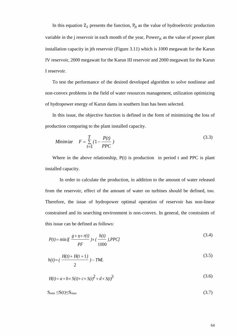
64

In this equation Z2 presents the function, Pjt as the value of hydroelectric production

variable in the j reservoir in each month of the year, Powerjt as the value of power plant

installation capacity in jth reservoir (Figure 3.11) which is 1000 megawatt for the Karun

IV reservoir, 2000 megawatt for the Karun III reservoir and 2000 megawatt for the Karun

I reservoir.

To test the performance of the desired developed algorithm to solve nonlinear and

non-convex problems in the field of water resources management, utilization optimizing

of hydropower energy of Karun dams in southern Iran has been selected.

In this issue, the objective function is defined in the form of minimizing the loss of

production comparing to the plant installed capacity.

T

t)

PPC

P(t)(FMinimize

11

(3.3)

Where in the above relationship, P(t) is production in period t and PPC is plant

installed capacity.

In order to calculate the production, in addition to the amount of water released

from the reservoir, effect of the amount of water on turbines should be defined, too.

Therefore, the issue of hydropower optimal operation of reservoir has non-linear

constrained and its searching environment is non-convex. In general, the constraints of

this issue can be defined as follows:

),PPC]h(t)

()PF

r(t)ηg[(P(t)

1000min

(3.4)

TWL))H(tH(t)

(h(t)

2

1

(3.5)

S(t)dS(t)cS(t)baH(t) 32 (3.6)

Smin ≤S(t)≤Smax (3.7)

65

Rmin ≤R(t)≤Rmax (3.8)

t)R(t)-loss(Q(t)S(t))S(t 1 (3.9)

r(t) = c(t)×R(t) (3.10)

In the above formulas, g is gravitational acceleration (in m/s2), power-plant

output, PF is plant factor, h(t) is effective water load on power-plant is calculated by

(using (3.5), H(t) is reservoir balance in the period t (a function of reservoir volume in

period t), R(t) is the water flow rate passing through the turbine in period t, S (t) is

reservoir storage at the beginning of period t, Q (t) is inflow amount into the reservoir in

period t, losst the lost amount in the period t, Rmin is minimum amount released from the

reservoir, Rmax the highest rate of release of the reservoir, Smin is the minimum allowed

reservoir storage, Smax is the maximum allowed reservoir storage, c (t) is conversion ratio

of passing discharge from the turbine (m3 / s), TWL is Tail Water Level, in order to

calculate the effective water load on the turbines, by using the information about reservoir

volume- height a third degree polynomial function is fitted by (3.6) which its constant

coefficients are listed below.

a= 878.7987956768

b= 0.1941700727

c= - 0.0001147356

d= 0.0000000270

The main factor in determining the optimal operation system of a dam - including

single dam and multiple dam - is the nonlinear relationship between hydropower energy

production, the amount of water released from turbines under uncertainty conditions of

input flows and the amount of demands for electrical energy (C.-T. Cheng et al., 2008;

Heydari, Othman, & Qaderi, 2015). The optimization model for planning operating

systems of multiple dams should reflect the exchange between the benefits obtained from

the storage and saving of the water and the benefits obtained from releasing the water. On

66

the other hand, there is an exchange between the benefits of storing water in high-level

and the loss resulting from the overflow of water. This study’s aim is to create and develop

a general flexible model which includes the structure and main features of the problem as

much as possible (Heydari, Othman, & Taghieh, 2016).

The third objective is flood controlling (Equation (3.11)). This function also presented

by minimizing the subtraction between the stated goal value; this ideal amount of volume

for flood control is considered 212 million cubic meters for the Karun IV reservoir and

2970 million cubic meters for Karun III reservoir and 2993 million cubic meters for the

Karun I reservoir.

𝑀𝑖𝑛𝑖𝑚𝑖𝑧𝑒 𝑍3 = ∑∑(𝑆𝑗𝑡− 𝑆𝑇

𝑗𝑡

𝑆𝑇𝑗𝑡

)

2𝑇

𝑡=1

3

𝑗=1

(3.11)

Z3 shows 3rd objective function, Sjt is the volume variable of the jth dam (Equation

(3.11)) and STjt is the goal volume in the jth dam for flood control. The constraints of this

relationship can also be included within the changing volume of each dam. “It is important

to note that for flood controlling model 6 months of a year is considered i.e. November

to April.”

3.3.2 The constraints of the problem

For optimizing the above-mentioned objective, we should consider different

constraints. The constraint related to the first objective function includes the scope of the

water release (Equation (3.1)). Besides this constraint, there is also another constraint

called overflow, which plays an important role. Overflow in the model is defined when

water surplus exceeds the maximum capacity of storage. Explicit lower and upper bounds

on storage for recreation, providing flood control space, and assuring minimum levels for

dead storage and power plant operation are expressed as follows:

Hj,t ≥ HeadMinj,t , 𝑗 = 1,2,3; (3.12)

Hj,t ≤ HeadMaxj,t, 𝑗 = 1,2,3; (3.13)

67

Rmin j,t ≤R j,t≤Rmax j,t , 𝑗 = 1,2,3; (3.14)

R2,t ≥ WRreqt (3.15)

𝐷𝑚𝑖𝑛𝑗𝑡≤ 𝑅𝑗𝑡

𝑑𝑒𝑚𝑎𝑛𝑑 ≤ 𝐷𝑚𝑎𝑥𝑗𝑡, 𝑗 = 1,2,3; (3.16)

𝑆𝑝𝑖𝑙𝑙 ≈ 0, 𝑗 = 1,2,3 (3.17)

Where, HeadMinj,t is the minimum head allowed for reservoir j at time t, HeadMaxi,t

is the maximum head allowed for reservoir j at time t, Rminj,t is the minimum discharge

allowed for the downstream of reservoir j at time t, Rmaxj,t is the maximum discharge

allowed for the downstream of reservoir j at time t and WRreqt is the water discharge

required at Karun III to satisfy water demand at time t.

Those limits maintain minimum desired downstream flows for water quality control

and fish and wildlife maintenance, as well as protection for downstream flooding.

Equation (3.18) to (3.20) are related to hydroelectric. One important constraint of the

relationship is related to the elevation of the reservoir to its volume, which is obtained

from and surface-volume-height curve.

𝑃𝑗𝑡 = 𝑓(𝛾, 𝜇, 𝑅𝑗𝑡𝑃𝑜𝑤𝑒𝑟, 𝐻𝑗𝑡), 𝑗 = 1,2,3; (3.18)

𝐻𝑗𝑡 = 𝑓(𝑆𝑡) (3.19)

0 ≤ 𝑅𝑗𝑡𝑃𝑜𝑤𝑒𝑟 ≤ 𝑅𝑗𝑎𝑙𝑙𝑜𝑤𝑎𝑏𝑙𝑒

𝑃𝑜𝑤𝑒𝑟 , 𝑗 = 1,2,3; (3.20)

Each of the three dams that are located in this area has a hydroelectric generating

station with 1000, 2000 and 2000-megawatt power, in the Karun IV, Karun III and the

Karun I dams, respectively. The variables of energy release from power plants and energy

production are considered in the modelling, which is the relationship between

hydroelectric release and the elevation of the reservoir. As will be discussed, the elevation

is counted in relation to the volume of the reservoir. This relation would be as follows

Equation (3.21):

𝑝𝑜𝑤𝑒𝑟 (𝐺𝑊ℎ) = 0.002725 × μ × RjtPower

(𝑚𝑐𝑚) × Hjt(𝑚) (3.21)

68

The units were set in a way that the achieved solution is in gigawatt-hours per month.

In fact the output and elevation variables are in the monthly average. In these equations,

Hjt is the water elevation above the turbine in jth reservoir, γ is specific weight of water,

μ is hydroelectric turbine efficiency and RjtPower is water release from hydroelectric

turbine. As for the constraint related to elevation, it should be noted that this equation can

be calculated by fitting a curve of the relationship which can be written in the form of a

third degree curve or in the form of another relationship, such as Power curve, etc. To

express the relationship between surface of the reservoir and its volume, the evaporation

from the surface of the reservoir should also be calculated. These equations change the

model from linear to non-linear.

Figure 3.12: Area-Volume-Elevation relationship for Karun IV reservoir

According to the elevation-storage curve of Karun IV reservoir (Figure 3.12), the

points are fitted by curve-fitting toolbox and power equation was used to calculate the

relationship. This relationship is defined as follows:

Mathematical Relationship Equation for Karun IV

22

11 )H 20.00014972+148(-110.5044V (3.22)

10.56739394

11 V 80.36587479 20.12979210 A (3.23)

840

860

880

900

920

940

960

980

1000

1020

1040

0 500 1000 1500 2000 2500 3000

Volume (mcm)

Ele

vati

on

(m

asl)

840

860

880

900

920

940

960

980

1000

1020

1040

05101520253035

Area (km^2)

Elevatio

n (m

asl)

Volume

Area

69

10.41234972

11 V 7.39836791 407301847.574447 H (3.24)

The correlation coefficients for fitting those equations to the data, are 0.999945779,

0.997632, and 0.99869621.

Figure 3.13 shows the elevation-storage curve of the Karun III dam and the physical

relationship equation were calculated using Equation (3.25) to (3.27):

Figure 3.13: Area-Volume-Elevation relationship for Karun III reservoir

Physical Relationship Equation for Karun III

23

22 )H 4180.00000020392(-68.78891 V (3.25)

70.32896663

22 V 913.1049582 2663.371983H (3.26)

60.66109414

22 V 0.2452244 50.03862441 A (3.27)

The correlation coefficients for fitting those equations to the data, are 0.999431047,

0.999489651, and 0.999850022.

Figure 3.14 shows the elevation-storage curve of the Karun I dam and it is calculated

by (3.28. to 3.30)

660

680

700

720

740

760

780

800

820

840

860

880

0 500 1000 1500 2000 2500 3000 3500 4000 4500 5000

Volume (mcm)

Ele

vati

on

(m

asl)

660

680

700

720

740

760

780

800

820

840

860

880

010203040506070

Area (km^2)

Elevatio

n (m

asl)

Volume

Area

70

Figure 3.14: Area-Volume-Elevation relationship for Karun I reservoir

Physical Relationship Equation for Karun I

23

33 )H 900.00000057677(-31.35212 V (3.28)

50.33643137

33 V 11.4338866 360.629964 H (3.29)

10.73144711

33 V 10.15313714 80.80039713 A (3.30)

The correlation coefficients for fitting those equations to the data are 0.999951298,

0.999885332, and 0.999034531.

Other provisions of the model which are common among all three objectives contain

the equation related to the confines of the reservoir storage, continuity equation

considering the waste of water which is the relationship between the surface of the

reservoir and evaporation rate.

𝑆𝑗𝑚𝑖𝑛≤ 𝑆𝑗𝑡 ≤ 𝑆𝑗𝑚𝑎𝑥

, 𝑗 = 1,2,3; (3.31)

𝑆𝑗𝑡+1= 𝑆𝑗𝑡 + 𝐼𝑗𝑡 − 𝑅𝑗𝑡

𝑑𝑒𝑚𝑎𝑛𝑑 − 𝑅𝑗𝑡

𝑝𝑜𝑤𝑒𝑟 − 𝐿𝑜𝑠𝑠𝑗𝑡 − 𝑆𝑝𝑖𝑙𝑙𝑗𝑡 , 𝑗 = 1; (3.32)

𝑆𝑗𝑡+1= 𝑆𝑗𝑡 + 𝐼𝑗𝑡 − 𝑅𝑗𝑡

𝑑𝑒𝑚𝑎𝑛𝑑 − 𝑅𝑗𝑡

𝑝𝑜𝑤𝑒𝑟+ (𝑅𝑗−1𝑡

𝑑𝑒𝑚𝑎𝑛𝑑 + 𝑅𝑗−1𝑡

𝑝𝑜𝑤𝑒𝑟− 𝐷𝑗−1𝑡

) − 𝐿𝑜𝑠𝑠𝑗𝑡

− 𝑆𝑝𝑖𝑙𝑙𝑗𝑡 , 𝑗 = 2,3;

(3.33)

𝐿𝑜𝑠𝑠𝑗𝑡 = 𝑓(𝐸𝜐𝑗𝑡 , 𝐴𝑗𝑡), 𝑗 = 1,2,3; (3.34)

𝐴𝑗𝑡 = 𝑓(𝑆𝑗𝑡 , 𝑗) = 1,2,3; (3.35)

350

370

390

410

430

450

470

490

510

530

550

0 500 1000 1500 2000 2500 3000 3500 4000 4500

Volume (mcm)

Ele

vati

on

(m

asl)

350

370

390

410

430

450

470

490

510

530

550

01020304050607080

Area (km^2)

Elevatio

n (m

asl)

Volume

Area

71

j,t j,t j, t-1 j,tEv (A A ) /2 EvRate (3.36)

j,t j,t j,t j,t j,tR RD DemAgr DemInd DemQual (3.37)

In these equations Lossjt is the water waste from jth reservoir, which is considered as

surface evaporation in this model. Ijt is the discharge of jth reservoir input in a year in

terms of million cubic meters. Rjt

power is the release to hydroelectric turbine for energy

production, as each turbine has an allowable amount of maximum design (Rjallowable

power)

which is mentioned in the constraints. Eυjt is the evaporation rate from the surface of

reservoir which is usually measured in millimeters. Ajtis the surface area of the jth

reservoir which is in non-linear relation to its storage. EvRate j,t is evaporation rate from

reservoir j at time t, RDj,t is the release from reservoir j and inflow to the downstream

reservoir at time t , DemAgrj,t is the agriculture water demand from reservoir j at time t,

DemIndj,t is the industrial and municipal water demand from reservoir j at time t,

DemQualj,t is the water demand from reservoir j at time t to satisfy water quality

standards.

Decision and State Variables

Decision variables are courses of action to be taken for each time period. In

optimization models which are developed in this study, the discharge of each reservoir j

at time t (Rj,t) are chosen as decision variables (control variables). Moreover, the

reservoir storage at time t (Stj,t) are considered as state variables.

The state variables are the variables describing the state of the system at any time t.

At any time t there are input state variables Stj,t and output state variables Stj,t+1.

The state variables of the system in the optimization model have the function of

linkage to the succeeding stage so that, when each stage is optimized separately the

resulting decision is automatically usable for the entire problem.

72

3.3.3 Data required for the models

1. Volume-area-elevation relationship for each reservoir Equation ((3.22) to ((3.30)

2. Hydropower characteristics (Discharge-Level-Hydropower production)

(Table 3.2)

3. Water Demand for agriculture in downstream of Karun III at time t)

4. Evaporation rates at each reservoir j at time t (Table 3.3)

5. Inflow rate at j location at time t with its probability

6. Hydropower production required at time t

7. Minimum water requirement at time t for water quality standards.

8. Initial value for volume at time 0 for each reservoir j.

73

Table 3.2: Hydropower characteristics

Karun I Karun III Karun IV

Reduction factor for dry periods(α) 0.91 0.94 0.92

Plant factor coefficient (PF) 0.17 0.14 0.16

Hours working hours in a power plant 4.1 3.4 3.8

Average inflow to the power plant (Qave) 27.3 123.0 211.3

Installed capacity (MW) (IC) 2000 2000 1000

Efficiency Hydropower Station (ep) 0.85 0.85 0.85

Percentage of Q used in Hydropower 1.0 1.0 1.0

Minimum allowable storage (Smin) 1675 1250 1441

Maximum allowable storage (Smax) 2997 2970 2192

Active storage 1322 1720 751

Minimum head for each reservoir (masl) 363 400 800.

Tail Water level (masl) 366 660 842

End Head at the end of planning period (masl) 400 800 985

Minimum operation level (WLmin) 500 800 996

Normal water level (NWL) 530 845 1025

Crest level (masl) 542 850 1032

Table 3.3: Evaporation Rate from Open Water surface in (mm per day) at time t

Month Karun IV Karun III Karun I

Jan 0 0 0

Feb 0 0 0

Mar 0 0 0

Apr 1.7 1.1 2

May 4.9 4.8 4.9

Jun 9.4 10 9.5

Jul 11.6 13 12.3

Aug 11.8 13.5 11.9

Sep 9.9 11.6 9.6

Oct 6.6 7.5 6.1

Nov 2 2.4 1.7

Dec 0 0 0

74

Table 3.4: Demand Irrigation (MCM) existing irrigation (partial)

Month Karun IV Karun III Karun I

Jan 0.00 0.83 0.00

Feb 0.00 7.00 0.00

Mar 0.00 15.58 0.00

Apr 0.00 38.60 0.00

May 0.00 87.04 0.00

Jun 0.00 179.76 0.00

Jul 0.00 196.95 0.00

Aug 0.00 140.60 0.00

Sep 0.00 94.25 0.00

Oct 0.00 52.25 0.00

Nov 0.00 23.11 0.00

Dec 0.00 5.12 0.00

For an average year reservoir inflows, the monthly optimization program is used with

existing partial irrigation, water supply, industry demands for all three reservoirs case.

Figure 3.15 represents the monthly reservoir inflows.

Figure 3.15: Reservoir Inflows

75

Output

A policy for release water from each reservoir j at time t for the certain

objective function.

Assumptions

Inflow is the only stochastic parameter

The water downstream reservoirs are almost near the channel level.

There is no time lag between each reservoir.

Optimization Engine Inputs

Inflows: There are the inflows into each reservoir at time t

Basic:

o The maximum head allowed at each reservoir at time t.

o The minimum head allowed at each reservoir at time t.

o The maximum Volume allowed at each reservoir at time t.

o The Minimum Volume allowed at each reservoir at time t.

o The maximum Area allowed at each reservoir at time t.

o The minimum Area allowed at each reservoir at time t.

o The maximum Discharge allowed from each reservoir at time t.

o The Minimum Discharge allowed from each reservoir at time t.

o It has the information for Initial water level for each reservoir,

o Final water level for each reservoir,

o Tail water level in each reservoir,

o the minimum water required for water quality standards,

o Efficiency Hydropower Stations,

o Percentage of Q used in Hydropower.

Losses-other:

o All losses except the evaporation rates (Seepage, bank storage, etc).

76

o The evaporation rates

Demand

o Agricultural demand at the downstream of each reservoir at time t.

o Industrial and municipal demand at the downstream of each reservoir

at time t.

o Other demands at the downstream of each reservoir at time t.

The users can examine the following scenarios:

Different inflows values and pattern for each reservoir.

Different hydropower efficiency.

Different water loses scenarios include different evaporation rates.

Different scenarios for Agriculture demand, Industrial and municipals

demand, and Power demand.

Different constraints regarding Maximum, Minimum Head and Volume

allowed for each reservoir for flood protection.

Different constraints regarding maximum and minimum area from reservoir

and discharge from each reservoir for environmental factors (fishes, soil

degradation, channel maintenance).

Different operation of selected set of reservoirs.

Several different scenarios had been tested successfully.

3.3.4 Description of the flood control

The Dams Operation Office has provided some classic flood control rules based

on peak discharge and flood volume. In order to work out the rules, instantaneous peak

discharges into the dam have been derived for different return periods. Then the inflow

flood volume has been assessed for different durations. A specific duration has been

determined for each dam by analyzing historical flood data. Return periods and flood

77

volumes are determined based on real time inflow peak discharges. Reservoir release is

subsequently determined from the known flood volume and the downstream catchment

flood and river safety capacity.

78

Operating Rules for flood control

Different rules can be defined for reservoir flood control depending on the simulation

objectives. Bearing in mind that the main object of the study is the downstream flood

mitigation plans, assumption which is compatible with planning of flood mitigation

projects has been considered. Downstream flood mitigation plans will be under safety by

considering critical operation rules at upstream reservoirs under any condition. In this

case the flood peak discharge magnitude is the maximum which the river system can

deliver. The following assumptions have been made for each element:

1. The reservoir is full and the initial level is the normal level when the flood occurs;

2. The control point defines downstream of each dam to determine releases;

3. Reservoir flood routing is accomplished by storage method;

4. The flood release is equal to the inflow discharge while the release peak discharge

does not exceed downstream safe capacity and the spillway capacity is sufficient

to release;

5. The release is limited to the downstream safety, capacity, and the reservoir water

level exceeds the normal water level (NWL) if the release from downstream

capacity is exceeded;

6. If the reservoir level exceeds the flood control level, the reservoir level must be

adjusted to flood control level. In this case, the reservoir release would be equal

to the inflow discharge if the spillway had no limitation in the capacity;

7. For the previous rule, if the release is greater than the spillway capacity, the

reservoir release is limited to spillway capacity and the reservoir water level

exceeds flood control level;

8. The reservoir discharges (up to the limit of downstream capacity) after recession

of flood until the reservoir level reaches NWL. After this moment, release is equal

to the inflow discharge and reservoir level is maintained at NWL.

79

Downstream safe capacity

In this study, the control point was immediately defined downstream of each dam

for the determination of downstream safe capacity. This factor is one of the most

important parameters involved in reservoirs flood control. Since the reservoir flood

control volume is defined based on the downstream capacity (or the most critical flood

damage areas of the river system), the downstream capacity was determined by designed

flood control volume, considering 100-year flood as the operational flood. The capacity

was calculated such that the reservoir flood control volume is filled based on the 100-year

flood without breach of the downstream capacity during flood release. Table 3.5 shows

the results of downstream capacity of the dams in existing situation including Karun IV,

Karun III and Karun I reservoirs as parallel dams.

Table 3.5: Downstream capacity of dams based on 100 year return period flood and

designed flood control volume (cms)

Existing situation Karun IV Karun III Karun I

2650 3750 4320

Reservoir Flood Attenuation

Figure 3.16 shows a schematic of the Dez and Karun river simulation model in

current condition. In the Karun river system, control points include Karun IV, Karun III,

Karun I, Upper Gotvand, Gotvand regulation dam and the confluence point of the Shoor

and Karun rivers.

80

Figure 3.16: Layout of flood control simulation

The delay time between the routed release flood hydrograph from the dams and

the intermediate flood hydrograph was determined so that the peak discharge of the

superposed hydrograph had a maximum peak discharge.

The downstream capacity was considered constant for another return period after

determining the downstream capacities, based on the 100-year flood. Reservoir flood

control simulation results are summarized in Table 3.6 to Table 3.8 for flood return

periods from five to 1000 years. Figure 3.17 to Figure 3.22 show the respective results of

the 100 and 200-year flood control simulation of different dams.

The reservoir flood control volume is not completely filled during floods with

return period less than 100 years because the inflow peak discharge is similar to the

outflow peak discharge and less than the downstream capacity. In contrast, with return

periods more than 100 years, the outflow peak discharge exceeds the downstream

capacity; hence, the reservoir flood control volume is filled by floods. During these flood

81

events, reservoirs retard the release peak discharge for floods below 100-year return

period.

Table 3.6: Flood peak discharge of Karun IV River

Flood return

period (year) K4 Inflow (m3/s)

K4 outflow

(m3/s)

K4 MOL

(masl)

K4-K3

intermediate flow

(m3/s)

5 1999.0 1999.0 1025.0 1669.0

10 2516.0 2516.0 1025.0 2100.0

20 3012.0 2650.0 1025.3 2514.0

25 3171.0 2650.0 1025.5 2646.0

50 3630.0 2650.0 1026.2 3029.0

100 4032.0 2650.0 1027.0 3365.0

200 4411.0 4054.0 1027.0 3680.0

500 4977.0 4903.0 1027.0 4153.0

1000 5500.0 5189.8 1027.1 4590.0

Table 3.7: Flood peak discharge of Karun III River

Flood return

period (year) K3 Inflow (m3/s)

K3 outflow

(m3/s)

K3 MOL

(masl)

K3-K1

intermediate flow

(m3/s)

5 2995.2 2995.2 845.0 997.0

10 3625.8 3625.8 845.0 1255.0

20 4419.0 3750.0 845.7 1502.0

25 4423.9 3750.0 845.7 1580.0

50 5050.2 3750.0 846.8 1809.0

100 5598.7 3750.0 848.0 2010.0

200 5804.5 5284.1 848.0 2199.0

500 6247.0 6247.0 848.0 2482.0

1000 6916.2 6916.2 848.0 2742.0

82

Table 3.8: Flood peak discharge of Karun I River

Flood return

period (year)

K1 inflow

(m3/s)

K1 outflow

(m3/s)

K1 MOL

(masl)

K1-UG intermediate

flow (m3/s)

5 3969.7 3969.7 530.0 1382.0

10 4849.1 4320.0 530.4 1739.0

20 5251.6 4320.0 531.1 2082.0

25 5329.9 4320.0 531.3 2191.0

50 5559.0 4320.0 531.8 2508.0

100 5758.5 4320.0 532.0 2787.0

200 7370.9 6889.1 532.0 3048.0

500 8637.0 8637.0 532.0 3440.0

1000 9576.3 9576.3 532.0 3801.0

Figure 3.17: 100 year flood control of Karun IV dam

83

Figure 3.18: 100 year flood control of Karun III dam

Figure 3.19: 100 year flood control of Karun I dam

0

1000

2000

3000

4000

5000

6000

7000

8000

0 20 40 60 80 100 120 140

Time (hr)

Dis

ch

arg

e (

cm

s)

520

521

522

523

524

525

526

527

528

529

530

531

532

533

Le

ve

l (ma

sl)Inflow Hyrograph

Outflow Hyrograph

Level

Inflow

Outflow

Reservoir level

84

Figure 3.20: 200 year flood control of Karun IV dam

Figure 3.21: 200 year flood control of Karun III dam

0

1000

2000

3000

4000

5000

6000

7000

8000

9000

10000

0 20 40 60 80 100 120 140

Time (hr)

Dis

ch

arg

e (

cm

s)

840

841

842

843

844

845

846

847

848

849

Level (m

asl)

Inflow hydrograph

Outflow hydrograph

Level

Inflow

Outflow

Reservoir level

85

Figure 3.22: 200 year flood control of Karun I dam

In the Karun River, the peak discharge at the outlet of Karun catchment after

superposition of Shoor river hydrograph is 3,495 and 10,010 m3/s for the 5 and 1000-year

return periods, respectively. Determination of the flood peak discharge in the flood plain

area involves hydraulic modelling because of the effect of flood routing in these areas.

Figure 3.23: Relations of flood control storage equivalent for a 100-year flood, the

interval Upper Karun

0

1000

2000

3000

4000

5000

6000

7000

8000

9000

0 20 40 60 80 100 120 140

Time (hr)

Dis

ch

arg

e (

cm

s)

520

521

522

523

524

525

526

527

528

529

530

531

532

533

Le

ve

l (ma

sl)

Inflow hydrograph

Outflow hydrograph

level

Inflow

Outflow

Reservoir

level

-2000

-1500

-1000

-500

0

500

1000

1500

2000

-2000

-1500

-1000

-500 0

500

1000

1500

Karun 4 Karun 3 Karun 1 Gotvand TR Karun 4 EQ Karun 3 EQ Karun 1 EQ

Flood peak reduction (cms)

FC (mcm)EQ FC (mcm)

EQ FC (mcm)

86

Figure 3.24: The relation between flood control reservoir storage in upstream and 100-

year flood in the upper Karun range

3.3.5 Description of the optimal cropping pattern

Water resources development projects with the aim of increasing area of water for

irrigation are of infrastructural plans that are considered in countries with arid and semi-

arid climate such as Iran. For designing an optimal cropping pattern in an irrigation and

drainage network, that has defined resources and restrictions, different methods are

available for managers and researchers.

One of the methods that is frequently used in the optimal allocation of scarce

resources is the use of mathematical programming models. Due to the special features of

the model parameters and variables such as crops, crop rotation, crop operations calendar,

calendar of common irrigation consequent, Wide range of agricultural crops cultivated

ingredients, limited arable land and product serious competition for water, the best way

y = 1.3554x + 116.78

R2 = 0.999

y = 1.3676x + 211.56

R2 = 0.9941

y = 1.078x + 112.1

R2 = 0.9955

0

200

400

600

800

1000

1200

0 100 200 300 400 500 600 700 800 900 1000

FC (MCM)

EQ

FC

(M

CM

)

Karun 4 EQ

Karun 3 EQ

Karun 1 EQ

Linear (Karun 3 EQ)

Linear (Karun 4 EQ)

Linear (Karun 1 EQ)

87

that encompasses information to guide in regulating water to their fields by the farmers

and also provides the optimization of these activities, is mathematical programming

models.

Linear programming patterns of the past decade and especially in the current era

were used to achieve the objectives of policy in some sectors such as agricultural sector,

determining the optimal combination cultivated and agricultural inputs, different patterns

cultivated and different ways to deal with water pollution that has been widely used to

estimate the demand for irrigation water.

Regarding the nature of the matter, applying linear programming is one of the

efficient and common methods. Therefore, most of the resources, restrictions, aims and

sensitivities of these kinds of matter that can be compiled with developing models based

on linear programming are considered for determination of an optimal cropping pattern.

Based on this, applying a program by using linear programming that includes all of

the above items requires designing a model that first includes three principles: aims,

variables, constraints and the relation between these principles should be defined in a

matrix called programming matrix. The designer can follow side goals in the framework

of variables and constraints by using linear programming in addition to final goals. The

conditional point in using this method at first is understanding the available relations

among aims, change resources, constraints and then domination on software and program.

After determining the optimum outflow value of the reservoirs, we must determine

the best cropping pattern in accordance to current conditions like water and land situation,

especially in the Karun III reservoir (because in downstream of the Karun III, the water

needs of agriculture are already defined.). Therefore, the first step should be specifying

area of fertile soil, then the conditions for proper drainage, cultivation and other terms are

88

being considered. Below is an overview of soil classification. In short, the methodology

is demonstrated in the following flowchart (Figure 3.25).

Figure 3.25: The flowchart of the cropping pattern and estimating the average

cost of agricultural products methodology

General Overview:

Brief descriptive notes on the land suitability classifications were provided by the

KWPA. These classifications appear to have been developed for use with the production

of annual crops, cereals and plantation of crops under gravity system of irrigation.

89

In determining the classification of lands for their suitability for irrigated crop

production consideration has been given to the following factors:

a) Topography: Slope (flat or steep) and Profile (undulating or level)

b) Soil properties: Physical (soil depth, texture, infiltration rate and

permeability of the sub-soil) and Chemical (pH, cation exchange capacity, proportion of

cations and anions and the saline and sodic status of the soil profile.)

c) Drainage: Potential for surface and sub-surface drainage

The analysis of the suitability of land for use in irrigated agriculture appears to have

been evaluated as a two-step process. The primary step has been the determination of

land classification classes, here in referred to as Land Suitability Classes, in which soils

are evaluated for use in irrigated agriculture. The second step appears to be the preparation

of Land irrigability Classes where more definitive definition of the suitability of the land

for irrigation is stated. A survey of the Salinity Classes has also been undertaken but no

tabulated data of the areas has been made available.

Determination of agricultural land suitable for irrigation

The standards for the classification of soils and land suitability have been developed

by a number of international and national agencies. The United States Department of

Agriculture established the initial set of criteria that has subsequently been expanded by

the FAO and other international agencies, thereby enabling the application of a consistent

set of standards for the classification of land. The maps and briefing notes provided

confirming that these standards have been applied to the surveys undertaken in the Dez

and Karun river basins.

Land Irrigability Classes: This classification system has been used to define the

level of management, resources and infrastructure required to enable sustainable irrigated

agriculture. The limitations made are based on the current standards of irrigation applied

90

in the Dez and Karun river basins and do not take into account the advances made

internationally in irrigation methods and management (Figure 3.26).

Class I – Irrigable: These are land areas without apparent limitations of soil,

topography or drainage or have limitations that can be fully corrected by land

improvements.

Class II – Irrigable: These areas are suitable for irrigated agriculture provided the

required land improvements are made.

Class III – Marginal Irrigable: These areas are expected to have marginal suitability

for irrigation even after the required improvements have been made.

Class IV – Restricted Irrigable: These lands are not suitable for irrigated agriculture

except under special conditions of land development, management and possibly only for

specific crops.

Class V – Undetermined Irrigable: These lands have severe limitations of soil,

salinity and/or drainage that will require considerable investment in soil improvement

works and evaluation of suitable crops.

Class VI – Non-Irrigable: These lands are not suitable for irrigation and have severe

limitations that require land improvements works that are not economically feasible.

After taking into consideration topography, soil properties and drainage,

agricultural land was categorized into six classes. In this study, only 2100 hectares of

agricultural land in the first class (Class I) that had the best agricultural conditions

(Table 3.9) was studied. The amount of water allocated to the mentioned land was about

six million cubic meters (MCM). Seventeen important agricultural products of the region,

namely Wheat, Barley, Husks, Corn, Pea, Lentil, Cotton, Sugar beet, Watermelon,

Cucumber, Potato, Onions, Tomatoes, Canola, Beans, Soya bean and rice were used for

the modelling.

91

Figure 3.26: The agricultural network

Table 3.9: The soil classification in downstream of Karun III (area in hectares)

Description Class

I

Class

II

Class

III

Class

IV

Class

V

Class

VI

Total

Reported

Karun III downstream 2100 10600 13400 440 21300 20960 68800

Total (Khuzestan) 931256

% of Total Area 0.23 1.14 1.44 0.05 2.29 2.25 7.40

92

Pre Modelling: Data needed for modelling were prepared in the form of constants,

values of the upper and lower limits and computational values in the pre modelling phase.

Table 3.10 shows the constants and constraints of the problem.

Table 3.10: Input amount of the problem (The data in this table is assumed only

for the case study and annual time distribution is considered)

Constants Constraints

Agricultural Products MWN APH PVT MAL MLN

(m3) (ton/ha) (1k Toman) (ha) (ha)

Wheat 4340 2.68 1050 400 374

Barley 3730 2.71 780 300 185

Husks 4180 4.25 850 40 24

Corn 5060 6.39 870 20 8

Pea 3940 1.05 1900 200 57

Lentil 4630 1.2 2000 200 59

Cotton 9160 2.37 2200 200 8

Sugar beet 4710 42.02 210 30 2

Watermelon 11850 27.69 374 40 3

Cucumber 3800 19.48 300 40 2

Potato 2970 29.03 300 40 3

Onions 4530 37.18 200 40 3

Tomatoes 1650 37.69 200 40 5

Canola 6590 2.08 1900 140 72

Beans 4930 1.67 1800 200 60

Soy spring 3220 2.34 1700 60 56

Rice 8890 4.23 2700 110 95

By using relations 3.41 to 3.43 computational values were obtained.

93

Computed values:

(Min water required to provide the desired capacity) i = (Min land

required)i * (Min. required water per hectare) (∀i = 1,2,3, … ,17).

(3.38)

Min land required for production = (Min tonnage i) /(Average

production per hectare i) (∀i = 1,2,3, … ,17).

(3.39)

Value per hectare i = (The product value per tonne) i*(Average

production per hectare) i (∀i=1, 2,3,…,17).

(3.40)

Therefore, the above relations can be written in the form of following mathematical

equations.

MWND i (m3) =

∏ (MWN (m3)∗ MT(ton))𝑖171

APH i (ton) (3.41)

MLN i (ha) = MT i (ton)

APH i (ton

ha)

(3.42)

VPH i (Toman) = ∏ (𝐴𝑃𝐻 ∗ 𝑃𝑉𝑇)𝑖171 (3.43)

94

Table 3.11: Computed value of problem (The data in this table is assumed only

for the case study and annual time distribution is considered)

VPH MLN MWND

(1000 Toman) (ha) (m3)

Wheat 2.81 374 1622430

Barley 2.11 185 688192

Husks 3.62 24 98260

Corn 5.56 8 39618

Pea 2 57 225143

Lentil 2.39 59 271213

Cotton 5.21 8 77332

Sugar beet 8.82 2 8967

Watermelon 10.35 3 19018

Cucumber 5.84 2 7803

Potato 8.71 3 10229

Onions 7.44 3 14623

Tomatoes 7.54 5 8757

Canola 3.95 72 475469

Beans 3.01 60 295210

Soy spring 3.97 56 179272

Rice 11.42 95 840861

Optimization Modelling and Implementation

The optimization problem was modelled with the aim of maximizing the ultimate

value of agriculture and subject to minimum water needed, the optimal agricultural land

and the minimum demand of the product (Equation 3.44 to Equation 3.45).

Objective Function:

Max Z = Σ(The optimal area of agricultural land for

production*Value per hectare) i (∀i = 1,2,3, … ,17).

(3.46)

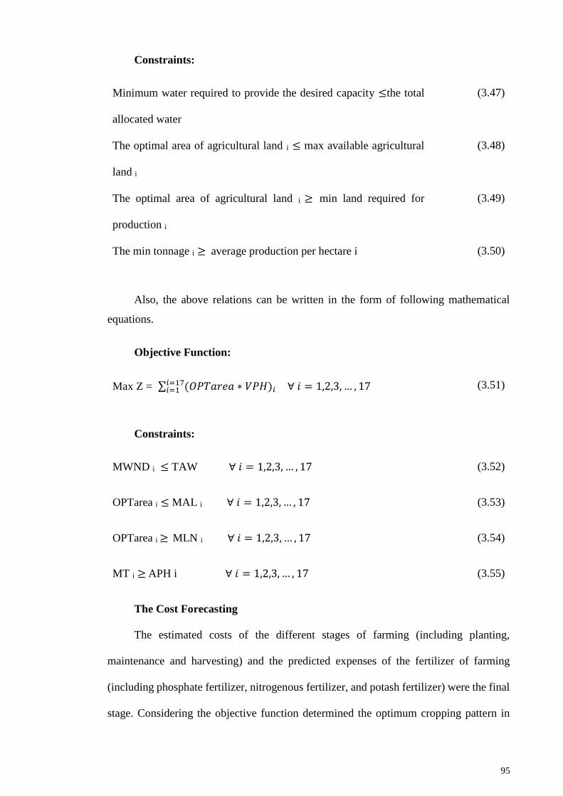
95

Constraints:

Minimum water required to provide the desired capacity ≤the total

allocated water

(3.47)

The optimal area of agricultural land i ≤ max available agricultural

land i

(3.48)

The optimal area of agricultural land i ≥ min land required for

production i

(3.49)

The min tonnage i ≥ average production per hectare i (3.50)

Also, the above relations can be written in the form of following mathematical

equations.

Objective Function:

Max Z = ∑ (𝑂𝑃𝑇𝑎𝑟𝑒𝑎 ∗ 𝑉𝑃𝐻)𝑖𝑖=17𝑖=1 ∀ 𝑖 = 1,2,3, … , 17 (3.51)

Constraints:

MWND i ≤ TAW ∀ 𝑖 = 1,2,3, … , 17 (3.52)

OPTarea i ≤ MAL i ∀ 𝑖 = 1,2,3,… , 17 (3.53)

OPTarea i ≥ MLN i ∀ 𝑖 = 1,2,3, … , 17 (3.54)

MT i ≥ APH i ∀ 𝑖 = 1,2,3, … , 17 (3.55)

The Cost Forecasting

The estimated costs of the different stages of farming (including planting,

maintenance and harvesting) and the predicted expenses of the fertilizer of farming

(including phosphate fertilizer, nitrogenous fertilizer, and potash fertilizer) were the final

stage. Considering the objective function determined the optimum cropping pattern in

96

terms of the number of acres of each crop, we can estimate and predict the cost of the

different stages of agricultural process. For this purpose, we must multiply the obtained

results of cultivation pattern in acre to cost breakdown values in tables taken from

ministry of agriculture (Table 3.12 and Table 3.13).

Table 3.12: The average consumed quantity and cost of fertilizer per acre

(Currency unit: TOMAN, Weight: Kg)

Fertilizer

Phosphate Nitrogen Potash Other Total

cost

per

kg

wei

ght

cost

per

kg

Wei

ght

cost

per

kg

wei

ght

cost

per

kg

wei

ght

cost

per

kg

Wei

ght

Wheat 78 152 66 232 61 18 126 8 72 410

Barley 75 152 60 180 64 9 120 9 68 350

Husks 109 249 43 398 92 22 349 11 65 680

Corn 83 144 73 331 77 19 286 7 81 502

Pea 79 48 62 50 54 6 179 0 69 104

Lentil 80 89 74 98 54 6 1500 0 77 188

Sunflower 81 162 73 215 60 26 133 5 76 408

Cotton 80 191 65 244 63 14 612 2 74 452

Sugar beet 94 246 73 275 66 45 128 23 83 589

Watermelon 91 187 75 194 81 16 184 46 90 443

Cucumber 92 254 79 411 82 56 205 70 90 791

Potato 89 269 81 361 69 70 316 12 90 713

Onions 99 233 94 333 67 28 185 29 98 623

Tomatoes 102 238 94 379 81 16 232 33 102 687

Canola 83 183 66 225 67 19 341 5 78 433

Beans 93 148 78 162 79 10 157 5 86 325

Soya bean 62 107 46 157 67 45 1582 3 67 311

Rice 136 162 102 219 71 27 189 3 114 412

97

Table 3.13: The average cost of producing one hectare of agricultural products

according to the different stages of farming (Currency unit: Toman)

Percent

Cost

Percent

Cost

Percent

Cost

Percent

Cost

Percent

Cost

Percent

Cost

Wheat

100

638649

30.3

6193888

11.3

272293

28.1

7179934

19.1

7122399

10.9

870135

Barley

100

556660

25.7

3143203

12.4

669340

30.4

1169267

18.5

9103487

12.8

271363

Husk

s100

2492794

26.9

6672075

12.4

3309817

28.7

8717548

21.2

528399

10.6

3264955

Corn

100

875784

32.5

284626

9.9

286917

35.6

3312030

13.1

4115041

8.8

177170

Pea

100

361688

22.7

882378

22.1

780204

27.9

100908

15.9

157556

11.2

440642

Len

til100

627963

21.7

8136774

26.8

168299

26.5

8166899

15.3

596394

9.4

959597

Sunflo

wer

100

1039942

21.2

7221172

20.1

209002

35.6

370252

14.0

6146246

8.9

793270

Cotto

n100

1156955

15.1

174699

21.5

5249301

45.9

5531586

10.6

9123656

6.7

277713

Sugar b

eet100

1418594

14.1

8201101

24.3

4345266

42.0

1595928

14.0

6199455

5.4

276844

Waterm

elon

100

1190808

16.7

6199613

26.1

3311186

27.9

3332545

19.4

5231559

9.7

3115905

Cucu

mber

100

2588252

12.8

4332278

31.9

2826160

28.8

6746842

20.1

5521644

6.2

3161328

Potato

100

2782335

12.7

7355286

17.1

9478416

22.9

1637528

43.6

31214020

3.4

997085

Onio

ns

100

2634561

13.7

360982

32.1

8847830

32.0

1843384

16.0

4422665

6.0

6159700

Tom

atoes

100

2964669

13.0

8387807

40.0

41187023

28.1

5834572

14.5

1430180

4.2

2125087

Can

ola

100

755590

33.6

6254338

9.8

474379

34.9

5264063

11.2

484911

10.3

177899

Bean

s100

1190464

23.0

5274446

19.2

9229585

34.1

4406442

16.6

8198524

6.8

481467

Soy

a bean

100

725466

39.4

5286180

11.6

784670

27.1

8197208

9.7

570760

11.9

486648

High

quality

med

ium

grain rice

100

2512094

29.3

4736960

14.4

9364078

23.9

6601820

21.7

3545799

10.4

9263437

Plan

ting

Farm

land

Prep

eration

The av

erage cost o

f pro

ducin

g one h

ectare of agricu

ltural p

roducts acco

rdin

g to th

e differen

t stages of farm

ing (U

nit: T

om

an)

0

Total

Farm

land

Harv

esting

Main

tenan

ce

98

Assumptions of the problem:

Important indices required for designing cropping patterns

Economic indices in cropping pattern should be determined in a way that with

selection of type of product along with increasing operation of available resources

(water, soil, etc.) we can achieve maximum revenue for farmers and producers;

and farmer can invest and develop their activities with increasing revenue and

interest of selling products and therefore we can observe economic flourish in

agriculture section.

Place of essential products in cropping pattern in designing the cropping pattern

should pay special attention to essential and strategic products such as wheat, corn

and oilseeds to supply food security of the state desirably and obtain self-

sufficiency for required products of the state.

Relative advantage of that group of agricultural products, which have more

advantages and higher economic desirability that they should be placed in

cropping pattern after essential products with priority.

Protecting basic resources and environment with the aim of stability in producing

agricultural crops, preserving basic resources (water, soil etc.) and environment

should be specially considered in designing cropping pattern.

Optimal consumption of water regarding this matter that the county is placed in

arid and semi-arid belt, cropping pattern should be designed by considering the

optimal operation of water resource.

Different parameters are involved in designing cropping pattern and selecting

plants for an irrigation and drainage system. Some of them are:

99

Government explained policies based on priorities of development and increasing

production of strategic products for meeting nutritional requirements of the state’s

population

Considering climate and soil of the region and its relation with compatibility of

agricultural plants

Creating variety in agricultural crops for controlling pests, diseases and weeds

Increasing soil fertility

Creating jobs in different seasons of the year

Operation of lands is possible

The quantity of irrigation water

Crop rotation

Crop water requirement

Economy of agricultural productions

100

3.4 A description of optimization methods

3.4.1 Genetic Algorithm

The genetic algorithm is an inquiry method and optimization based on principles of

natural evolution. This method is among the optimal optimization algorithms, which are

able to find the optimal solutions or the solutions close to them.

As the generation is done by a set of chromosomes and therefore Human traits are

inherited through the generations, GA mimics this natural behaviour and chooses the best

solution to be the parents of the next generation. This method produces several

generations of feasible solutions, which try to move toward the optimum.

In the GA initial population of solutions (chromosomes) is selected randomly to be

evaluated through objective functions and the constraints. A set of chromosomes is

chosen from the initial random population, whose objective function value is better than

the others. This set is assigned to be the parents for the next generation of chromosomes.

The new offspring of new parents replaces inferior chromosomes from previous

generations and therefore the next generation is formed. This is done until the last

generation reaches the optimum solution.

Process:

1. A random population of n chromosomes is generated.

2. Each chromosome in the population is evaluated in the fitness function

3. A new population is created by repeating the following steps

Two parent chromosomes are selected from a population according to their

superiority.

With certain probability function, the two parents are mated and new offspring

is produced with the aid of crossover function.

Mutation is applied and the offspring may change.

New offspring in the new population replaces inferior ones.

101

4. New population acts as the next generation in the next step of the algorithm.

5. The algorithm stops if the termination conditions are met. Therefore, the algorithm

returns the best solution.

6. Step 2 is repeated.

Genetic algorithm allows a population composed of many individuals who have been

made during a special selection rule; fitness function would be optimized during the

process of evolution. This method was developed by John Holland in 1975. Then, his

findings were generalized in order to solve some problems such as operation of the gas

pipeline by one of his students, David Goldberg in 1989. In the book published by him

which has been one of the most comprehensive sources in the genetic algorithm field, the

merits of this algorithm is comparison with the other methods are stated as follows:

Capability of optimization in continuous and discrete spaces

It does not require any information about derivate function

It is able to work with a large number of decision variables

It is possible to optimize very complex objective functions by using this algorithm

To begin, instead of using a single value, it uses a population with potential

solutions

It provides a possibility to use coded values of variables instead of using them

It uses probable rules than certain rules to guide the searching process

This algorithm is able to find the optimal solutions in many cases that traditional

optimal methods are unable to do. However, it should not be thought that genetic

algorithm is a good way to solve all the optimization problems. For instance, to find the

optimum point of a curve, which has just a point of absolute minimum or maximum,

classic methods which work based on derived, can find this point very easily and very

fast. Nevertheless, genetic algorithm may need double time compared to the classical

methods to find the answer. However, for functions that have many local extremum

102

points, definitely a classic method will have a problem, while, genetic algorithm will

comprehensively search the answer space, therefore, and the probability of convergence

in local optimum is very low.

Limitations of Genetic Algorithms:

1. If wrong evaluation function is selected, are may not get the correct answer.

2. Population size, mutation and crossover rate may directly affect the performance

of the algorithm. Therefore, setting the right values of these parameters is vital.

3. Another problem that is often seen in small populations, i.e. if one chromosome is

significantly away from most of its generation or is much better than others, it may result

in early convergence and lead to a local optimum solution.

Mechanisms of Genetic Algorithm

Genetic Algorithm begins with creation of an initial population of chromosomes. In

other words, chromosomes are series of suggested values for the problem decision

variables and each of them represents one probable solution for the problem. In the next

part, these chromosomes will be evaluated due to the objective of optimization and the

chromosomes will be considered the better solution for the mentioned problem, and have

more chance to reproduction for problem solution. Formulation of a fitness function of

chromosomes, accelerating the computing of convergence speed toward the global

optimum solution is very important, because the amount of fitness function must be

calculated for each chromosome in genetic algorithm and since we encounter many

chromosomes in many problems, calculation of the evaluation function is time

consuming. For some problems, application of genetic algorithm is practically

impossible. The genetic algorithm process is an iterative process, as the number of

chromosomes in the initial population is divided into two groups in any iteration; selected

and dropped which the next generation will be created of selected chromosomes. During

103

the process of generation iteration, different operators of the algorithm are playing to

reach the stopping criterion.

Genetic Algorithm Operator

After selecting the initial population of the algorithm, which is debated a lot, the

following operators are applied to the algorithm in order.

Evaluation:

As it was mentioned, each chromosome is representative of a series of solutions for

the optimization problem. After selecting the initial population, every chromosome must

be evaluated in the fitness function which is the objective function of the model and its

output amount from the fitness function must be compared with the amount of other

individuals of the population (chromosomes) and the best will be selected among these

amounts due to an objective model (maximum or minimum).

Crossover

Crossover is the most important operator in genetic algorithm. While operating this

operator, population of old generation have combined with each other and created new

generation. This function gradually diminishes population distribution during iteration of

generations, because the superior individuals combine to each other in any iteration and

since the criterion for superior individuals is to move to the optimal solution, the

distribution will be as low as possible.

Mutation

This operator plays an important role to search all the parts in the possible space,

because changing of the amount of some genes in each individual of population, makes

it also possible to search blind spots of possible space and it may cause the individuals

who have been changed their genes, find the possible solution faster. This operator

performs much effectively and is helpful in the large-scale problems (Figure 3.27).

104

Genetic algorithm

Figure 3.27: Genetic algorithm flowchart

NSGA II:

If there is more than one objective function then the problem will be complicated.

For example if one wants to build a structure that is both light and stiff, since these two

features are in contrast, we can look for alternative designs and relationships. Thus, there

would be the lightest and the most difficult design as well as an infinite number of plans

that are in compromise between stiffness and lightness. These sets of so-called alternative

designs are known as Pareto-Sets. Also with the help of the best chosen designs, we can

draw the trade-off curves that are obtained by plotting the weight against stiffness.

Figure 3.28 presents the answers to a double-objective problem of minimizing. Pareto

is described as a point that each of its corresponding objective values shouldn’t be worse

Choosing the parents based on fitting

function

Random creation of population in the

possible range

Define population size, selection

probability values, mutation

Applying crossover operator and

offspring reproduction

Fitting each child according to the

evaluation function

Applying mutation operator for the selected

genes of the new generation

Selecting the best individuals and

comparing them to other individuals

Continue

NO

Stop

YES

105

than the rest of the points or at least one corresponding objective of this point should be

better than the other answers. This point is referred to as Pareto or non-dominated, and a

set of answers related to these are called a set of Pareto (In Figure 3.28 the blue point are

Pareto and the white points are dominated answers of the problem). In this relationship,

same as the single-objective optimization, there are two approaches: classical methods

and evolutionary algorithms. However, there is a great difference between the two

approaches.

Figure 3.28: Non-dominated answers in Pareto range

Different classical methods which are based on mathematics and mathematical

derivations are described below. The mathematical equation of a multi-objective problem

can be defined as follow:

𝑀𝑖𝑛𝑖𝑚𝑖𝑧𝑒 [𝐹𝑖(𝑥), 𝐹𝑖(𝑥), 𝐹𝑖(𝑥)]𝑇 (3.56)

Subject to (3.57)

𝑔(𝑥) ≤ 0, (3.58)

ℎ(𝑥) = 0, (3.59)

𝑥1 ≤ 𝑥 ≤ 𝑥𝑢 (3.60)

Fi shows ith objective function, g(x) and h(x) are equal and unequal constraint

functions, respectively. [x] is the vector of problem’s decision variables.

The first objective

Th

e se

con

d o

bje

ctiv

e

106

3-4-2 Evolutionary approach based on sorting

In the past two decades, a number of multi-objective evolutionary methods have been

proposed. Among these methods the genetic algorithm with non-recessive sorting of the

solutions, has been one of the successful and promising approach. The first non-recessive

sorting of genetic algorithm (NSGA) was introduced by Srinivasa and Deb in 1994. The

algorithm was capable of obtaining any number of Pareto optimal solutions in each

implementation. NSGA-II is the developed version of the first method and it was

introduced to deal with the complexity of computation and diversity of the problems. The

algorithm consists of five major stages: forming the initial population, sorting non-

recessive solutions, crossover, mutation and eugenics.

This algorithm consists of following steps:

1. Random creation of the initial population so that the population lies in the possible

range. Then there is the evaluation of the population in the objective function and

the sorting of the non-recessive solutions, so that the population is changed into

several subsets, each with different ratings (For example, number 1 is assigned to

the first set of the non-recessive solutions, number 2 to the next set and etc.).

2. Crossover implementation for the selected population and the race selection

operators (which is normally half of the initial population, value of the ratio is

defined at beginning of the algorithm). To produce the next generation so that the

total population is the same as the initial population.

3. Evaluating the offspring’s cost function and repeating the sorting of the non-

recessive solutions and classifying the population based on the present ratings.

4. Selecting the new parents and producing offspring, implementing the mutation

and crossover operators and then evaluating the cost function again.

5. Repeat step 3 and 4 until the stopping criterion for the algorithm is met.

107

6. Since this algorithm is introduced for non-constraint optimization models,

the penalty function is used for writing and including the problem constraints.

Continuity constraints of the reservoir are the most important constraints

dominating the problem. In other words the procedure of this algorithm is shown

in the flowchart below (Figure 3.29):

𝐹1

𝐹2

𝐹3

𝑃𝑡+1

Figure 3.29: Genetic algorithm with non-recessive sorting of solutions

1. Randomly produced parent generation P0 in N numbers.

2. Classifying the first generation of the parents based on non-dominated solutions.

3. Considering an appropriate order with non-dominated level for each non-

dominated solution (1for the best level, 2 for the next best level after 1and etc).

4. Offspring reproduction Q0 in Nnumbers by using the selection, crossover and

mutation operators.

5. Considering the first reproduction, which is consisted of parent and offspring

chromosomes, the next reproduction is as follow:

𝑄𝑡

𝑃𝑡

Dominated

chromosomes

Classifying based on

distance Classifying based on non-dominated

solutions

108

a. Composition of parent Pt and offspring Qt chromosomes, and reproduction

Rt in 2N numbers.

b. Classifying Rt generation based on non-dominated method of sorting and

identification of non-dominated mantles (F1, F2,…,Ft).

c. Parent reproduction for the next iteration Pt+1, using produced non-

dominated fronts in N numbers. In this stage, due to the number of required

chromosomes for the parent generation N. At the beginning the first front

chromosomes for the parent generation is chosen, and if this number of

chromosomes are not enough for the total number of required

chromosomes for the parent generation, then they are harvested step by

step from 2,3 and… fronts until it reaches the total number of N.

d. Applying crossover operators, mutation on the regenerated parent

generation Pt+1 and regenerating the offspring generation in N numbers.

6. Repeating step 5 to achieve the total number of iterations.

3.4.2 Particle swarm optimization algorithm

The particle swarm optimization algorithm was first introduced by Kennedy and

Eberhart in 1997 (Kennedy & Eberhart, 1997). PSO algorithm is an evolutionary

computation that is inspired by nature and is based on iteration. The algorithm is inspired

by animals’ social behaviour, mass movement of birds and fish. Hence, PSO begins with

initial random population matrix like other evolutionary algorithms and imperative

competitive algorithm. Unlike genetic algorithm, PSO does not have any evolutionary

operators like mutation and crossover, therefore imperative competitive algorithm is more

similar to PSO than GA. Each element in the population is called a particle (same as

chromosome in GA, or a country in an imperialist competitive algorithm). In fact, PSO

algorithm is consisted of a certain number of particles, which randomly have initial

values. Two values of position and velocity are defined for each particle, which are

109

modelled with position and velocity vectors, respectively. These particles iteratively

move in −N dimensional space in order to calculate the optimal value as a criterion for

measuring to find possible new options. The dimensional space of the problem is equal

to the number of existing parameters for optimization in a function. A memory is allocated

to storing the previous best position of the particle and one memory is allocated to storing

the best-known position of best particle among all the particles. The experience from

these memories determines the movement of the particles in the next turn. In any iteration,

all particles move in the −N dimensional space of the problem to finally find the common

optimal point. The velocity and position of the particles are updated based on the best

local and absolute solutions. In PSO algorithm, the xi particle is updated as follow:

𝑥𝑖 (𝑡) =𝑥𝑖 (𝑡 − 1) +𝑣𝑖 (𝑡) (3.61)

𝑣𝑖 (𝑡) represents the velocity vector, and is calculated by the following equation:

𝑣𝑖 (𝑡)= 𝜔.𝑣𝑖 (𝑡 − 1) + 𝐶1. 𝑟1 − (𝑥𝑝𝑖 −𝑥𝑖 ) + 𝐶2. 𝑟2. (𝑥𝑔𝑖 −𝑥𝑖 ) (3.62)

In this formula xpi is the best solution that xi had in any iteration and xgi as the best

particle among all particles in any iteration. This particle is referred to as the leader. ω is

the inertia weight for particles that keeps the balance between local and global experience.

r1 and r2 are uniformly distributed random numbers in [0 and 1] interval. C1and C2as

specific parameters, control the best local and absolute particle. Particles move in the

search-space near the best absolute solution (leader) and do not explore the rest of the

space; this is called convergence. If a small velocity inertia coefficient is chosen, then all

the particles can reduce their speed until their speed is near zero in the ‘best local’.

The PSO algorithm (Figure 3.30), updates the velocity vector of each particle and

adds the new speed to the position and the value of the particle. Updating the velocity is

influenced by both best local and absolute solutions. The best local and absolute solutions

are obtained by one particle and the whole population until the algorithm is running.

C1and C2 invariants are perceptual and social parameters, respectively. The main

110

advantage of the PSO is that, it is easy to implement and it needs to provide only few

parameters. Moreover, PSO is able to optimize complex cost functions with many of local

minimum.

111

Figure : Particle swarm optimization algorithm flowchart

Figure 3.30: Particle swarm optimization algorithm flowchart

3.4.3 HPSOGA

The particle swarm algorithm was inspired by the collective movement of organisms

such as birds and fish. A population of particles is used in the algorithm that explore the

possible space to find the optimal answers. Each particle has a position and initial speed

in the population. In addition, each particle recalls the best position that it has previously

attained. Genetic Algorithm and Particle Swarm Algorithm ability to solve complex

problems has been proven several times. However, each of these two methods has weak

and strong points, the comparison between the genetic algorithm and particle swarm

Evaluating the fitness function for

each particle’s location

Definition of population and parameters of the

algorithm such as (C1 and C2)

To equalize the best experiment of

Pbest with Gbest parameter

Randomly generated particles in the

possible searching space

Updating the position vector and

velocity vector of particles according

to the mentioned formula

If the value of P fit is better than the

value of Pbest fit then Pbest=P

Stopping the algorithm and

presenting the Gbest as the best

answer

Iter

atio

n c

hai

n t

o t

he

last

val

ue

112

algorithm was done by Eberhart and Anjlayn and according to studies conducted by them,

it is suggested that by the combination of these two algorithms, the obtained model

converted into a model with strong performance in solving problems and creating a good

searching environment. The main objective of this paper is combining Genetic Algorithm

and Particle Swarm algorithms and general principle of this method is that the benefits

of particle swarm algorithm with very useful operators of genetic algorithm (mutation

and crossover) are combined and create hybrid algorithm (Angeline, 1998). One of the

advantages of the particle swarm algorithm compared to the genetic algorithm is

simplicity and having less parameters, another obvious difference is in the ability to

control the convergence to the optimal answer, the operation rate of mutation and

crossover can help in a good way to the convergence of genetic algorithm. However, these

operators are different from speed, weight-damping operator in the particle swarm

algorithm, and in fact, the convergence of the algorithm will be increased by decreasing

the effect of the weight over successive iterations. One of the major problems of particle

swarm algorithm is premature convergence and this convergence is not necessarily the

way to achieve the optimal solution, to prevent this happening, the position of the particles

and global best must be changed, and changing the situation is done by the combination

of genetic algorithm. Very efficient operators of genetic algorithm are mutation and

crossover operators that information is exchanged between two particles of the population

by applying the crossover operator. In this way, the desired particle can be transferred to

a new point in the context of the decision. The purpose of applying the second operator

(mutation) is to increase diversity and creating diversity in population and ultimately

preventing to achieve local optimal answer.

If the searching environment is D-dimensional, in this case, the initial positions

of each particle will be shown by the D-dimensional vector Xi = (xi1, xi2, ... xiD) and its

initial velocity by Vi = (vi1, vi2, ..., viD). Also, the best position of the particle and the

113

best position that the group have experienced, have been shown, respectively, by Pi =

(pi1, pi2, ..., piD) and Pg. In this case, the position and velocity of the particle can be

expressed by two following equations:

)()(VV 2211

n1n n

i

n

g

n

i

n

i XPrCXPrC

(3.63)

1n

i

n

i

1n

i VXX (3.64)

Where n is the number of repeats, c1 and c2 are constant coefficients that are called

cognitive and social parameters, respectively, and r1 and r2 are random numbers in the

range of 0 and 1. In fact, these two relationships represent an early version of particle

swarm algorithm. In this algorithm, there is no mechanism for controlling the speed of

the particles. Therefore, the velocity of the particles increases in an uncontrollable way.

This causes that particles pass beyond the appropriate answers. For this reason, different

methods are used to control the particle velocity. One of these methods is to apply the

maximum value for the speed. In this way, if the velocity of the particles were higher than

this amount, the maximum speed would be considered. Another method, which is more

common, is the use of factor “w” as weight inertia. If this parameter is used, the

Equation 3.65 will be as follows:

))()(V(V 2211

n1n n

i

n

g

n

i

n

i XPrCXPrCw

(3.66)

c1, c2 and w are obtained through the following relationships. In the above equation,

λ is the contraction coefficient (Clerc, 1999) and the purpose of using it to ensure the

convergence of the algorithm. How to get this coefficient is below.

W(n) = wmax – (n / iter max) (w max – w min) (3.67)

Where wmax and wmin are the inertia in the beginning and end of the process,

respectively. n is the number of iteration times of the algorithm so far, and itermax is the

total number of iterations in the algorithm.

114

Chromosome are randomly modified to increase their appropriateness in the genetic

algorithm. There are two basic solutions to this. The first solution is to use a crossover

operator which the process is simulated based on the combination of chromosomes during

reproduction in the living organisms. And the second solution is the use of mutation

operator.

Gene diversity and variety will be effectively improved by the two operators and

these two operators can be used in the particle swarm algorithm to improve the efficiency

of it. The flowchart of the combination of these two algorithms is presented in

Figure 3.31.

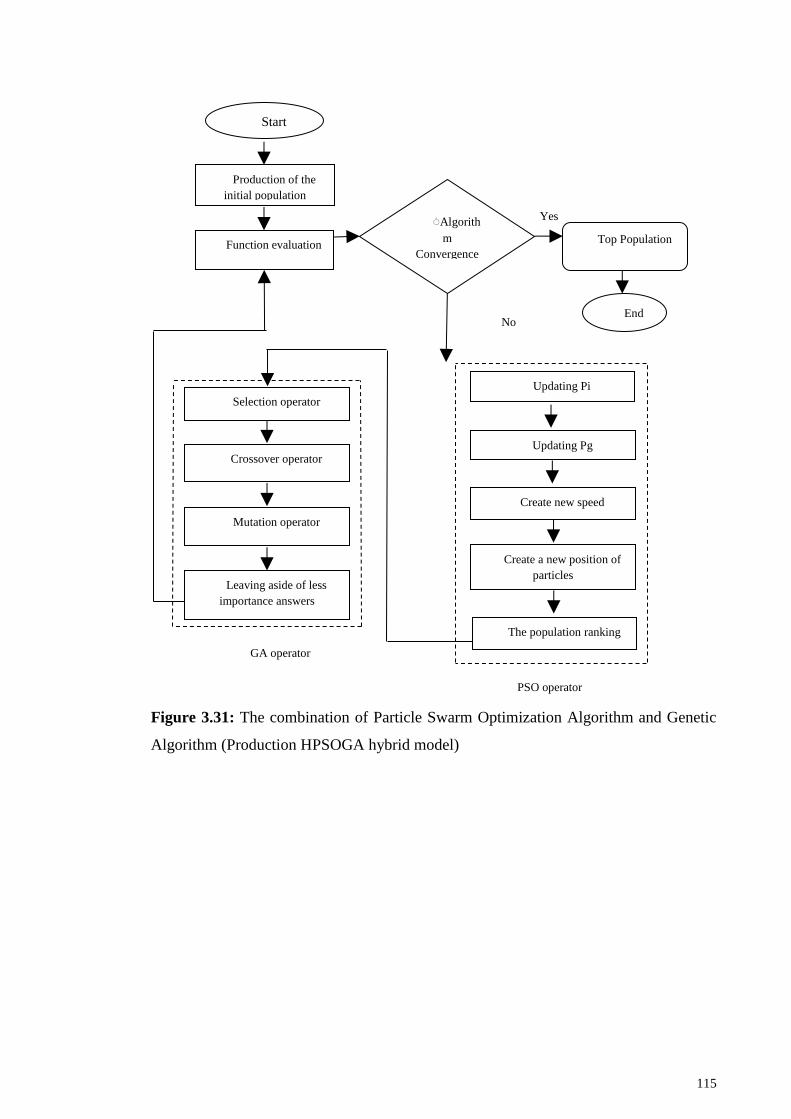
115

Figure 3.31: The combination of Particle Swarm Optimization Algorithm and Genetic

Algorithm (Production HPSOGA hybrid model)

PSO operator

The population ranking

Create a new position of

particles

Create new speed

Updating Pg

Updating Pi

No

Yes Algorith

m

Convergence

Top Population

End

Function evaluation

Start

Production of the

initial population

GA operator

Leaving aside of less

importance answers

Crossover operator

Selection operator

Mutation operator

116

3.5 A description of computational tools

3.5.1 LINGO

Lingo is a powerful tool for linear and nonlinear optimization to solve and analyse

formulated models of major and minor issues. Optimization helps to achieve the best

result, and highest profit, outcome or satisfaction or attain the least cost, losses or

dissatisfaction. These issues often include efficient use of the resources (the best way

possible) which consists of money, time, machinery, staff, stock, etc. optimization issues

are divided into two categories: linear and nonlinear, depending on whether the relations

between the variables are linear or not.

Generally, each optimization model includes the following three items:

Objective function: It is a formula expressing what exactly should be optimized.

Variables: They are quantities, under control and their best values are to be decided.

Constraints: Almost without exception, some limits can be considered on the amounts

of variables in a model (At least one resource is limited, such as time, raw materials,

budget, and etc.) these limits that are expressed as formulas which are a function of model

variables, are known as constraints.

Objective function 1:

The purpose of performing the optimization model in the cropping pattern is to

maximize the income, therefore; the objective function is defined as follows:

MAX: Z= ∑ (𝐶𝑗 . 𝑋𝑗)𝑛

𝑗=1

(3.68)

Subject to

∑ (𝑎𝑖𝑗 . 𝑋𝑗)𝑛

𝑖=1≤ bi i=1, 2….m

(3.69)

Xj≥0 (3.70)

Where:

117

Z: Objective function

Xj: Activities related to the production of various agricultural products

Cj: The coefficient matrix of the objective function

aij: Matrix of technical coefficients of production factors

bi: constraints’ values

Xj≥0: indicating the positivity of variable values

3.5.2 Solver in Excel

The described model was resolved by Linear Programming (LP) in Microsoft Excel

(Solver).

Excel solver is a powerful tool for optimization problems. This solver can solve

most of optimization problems like linear, nonlinear and integer programming. This tool

was first created by Frontline Systems, Inc (Fylstra et al., 1998). Excel solver uses

Generalized Reduced Gradient (GRG2) algorithm in order to optimizie nonlinear

problems and also uses the simplex algorithm for solving linear programming (Del

Castillo, Montgomery, & McCarville, 1996; Kemmer & Keller, 2010). The aim of linear

programming is to maximize or minimize the objective function of the farm’s manager

regarding some of the constraints (available resources) and decision variables (activities)

simultaneously.

118

3.6 A description of performance measures

3.6.1 RMSE

RMSE is often applied for measuring the difference between observed and calculated

values. One advantage of normalizing the RMSE is that it facilitates the comparison

between the datasets or models with various scales. The term coefficient of variation of

the N, CV (RMSE) might be used to prevent vagueness, during the normalizing by the

mean value of the measurements.

RMSE = √∑ ∑ (𝑦0−𝑦𝑐 )2

𝑁𝑖=0

𝑃𝐽=0

𝑁𝑃

(3.71)

NRMSD=𝑅𝑀𝑆𝐸

𝑋𝑚𝑎𝑥−𝑋𝑚𝑖𝑛 (3.72)

CV(RMSE)= 𝑅𝑀𝑆𝐸

�� (3.73)

Where Y𝑜 is the ith observation data (Lingo results) and Y�� is ith computed data (The

optimal solution obtained by evolutionary algorithm ( .�� is a mean of the data.

3.6.2 Regression

Regression Method

One of the most widely used statistical methods in different science fields is

implementation of regression techniques to determine the relationship between a

dependent variable with one or more independent variables. The dependent variable,

response and independent variables are also called explanatory variables. A linear

regression model assumes there is a linear relationship (direct line) between the dependent

variable and the predictor. Running a regression model is possible by defining the

regression model. The linear regression model with the dependent variable Y and

independent variable p x1, x2,..., xp is defined as follows (Tunçal, 2010):

yi = b0 + b1xi1 + … + bpxip + ei (3.74)

119

Where

yi: is the amount of ith dependent variable

p: is the number of predictors

bj: is the amount of ith coefficient, j = 0,..., p

Xij: is the value of ith of jth predictor

ei: is the observed error of the value for ith

The model is linear because the value of dependence of bi is increased by increasing

predictive value -ith. b0 is the intercept, that when any predictive value is zero, the value

of predictor model b0 is the dependent variable. In order to test hypotheses about the

values of model parameters, linear regression model also takes into consideration the

following assumptions:

• The error term has a normal distribution with a mean of zero

• The variance of the error term is constant in all cases and it is independent of the

variables in the model. (An error term with inconstant variance is called heteroscedastic).

• The amount of the error term for a given amount is independent of the variable

value’s in the model and is independent of the amount of error term or the other cases.

In the present problem, amount of inflow to dam (I) and Karun dam storage capacity

(S) are independent variables and the release from dam (R) value is a dependent variable.

3.6.3 Artificial Neural Network

Although regression models are still used to water resources problems such as

exploring the internal relations, prediction of weather and climate elements (Christensen,

Jian, Ziegler, & Demonstration, 2000; Piao et al., 2010), today, with the progress of

science and innovating some intelligent methods in different sciences, predictions of

120

various parameters is done using more intelligent methods such as artificial neural

networks. These networks have a great ability in modelling and prediction of weather and

climate elements. Creating an Artificial Intelligence system that can learn and have the

flexibility of human being is the main purpose of research in artificial intelligence. Trying

to imitate the human process has faced intensive activities in the past, which is followed

by world research centres through in-depth and purposeful studies nowadays. Many

models of intelligent biological systems are evolved during this period, which the goal of

each of these models has been to act as the brain and nerve system of humans. Particularly

research has been done from purely theoretical research into applied research, in

information processing which is no solution or in hard problems. Due to this issue, the

growing interest has been created in the development of intelligent, dynamic systems of

unlimited model based on experimental data. Artificial Neural Network which is called

Simulated Neural Network and or typically called neural networks too, are among these

dynamic systems that transfer knowledge or the underlying rule in data to network

structure through processing empirical data. That is why these systems are called

intelligent, because they learn general rules based on calculations of numerical data.

These networks are trained to overcome the limitations of conventional methods

to solve complex problems. These networks have shown very high performance regarding

Estimation and Approximation. In fact, wherever estimation, prediction, classification

and control are necessary, neural networks have been proposed there in different forms.

Intelligent neural networks have been successfully and widely developed to solve a very

wide range of issues. The scope of application of mathematical models based on the

performance of the human brain is very broad which can be mentioned as a small sample

of using the mathematical tool to predict the weather (Faridah Othman, Sadeghian,

Heydari, & Sohrabi, 2013).

121

The major component of a neural network is called a cell. Essentially biological

cells are combined with each other in different ways through receiving input from some

sources and then they offer the final output by doing non-linear operations on the inputs.

Neural networks often include one input and one or more intermediate layer (hidden

layer), and an output layer. Each entry is multiplied by the weight of its own. In the

simplest case, bias and outputs are added together and then pass through activation

function to produce outputs. These systems are trying to model the brain structure of the

Nero-synaptic based on computational intelligence. Figure 3.32 shows processing

information in a real and artificial cell of neural networks simultaneously.

Figure 3.32: The real neural schematic cell and artificial neural network

Activation functions are generally made of linear or nonlinear algebraic equations.

The most important step in the neural network is the training part of the network. In

general, there are two ways for Network training, which include controllable and

uncontrollable training. The most common training algorithm is training algorithm after

propagation. The neural network is trained through the algorithm after propagation by

changing the weight of the intermediate layer and these changes are stored as data

network.

122

Multilayer Perceptron (MLP): Multilayer Perceptron networks are a type of of

feed forward neural networks, which are one of the most used of models of artificial

neural network in modelling and prediction of climate elements. Several layers of neuron

in each layer are connected to all neurons of the previous layer in the Multilayer

Perceptron network. Such networks are called fully connected network. Regarding the

issue of estimation of atmospheric elements, Multilayer Perceptron networks have been

repeatedly used in different studies by the researchers because of train-ability and high

learning ability.

Implementation method:

The overall structure of the neural network model consists of three layers:

1. Input Layer: in this layer, the input data is introduced to the model.

2. The Hidden Layer: in this layer the information is being processed.

3. Output Layer: The results of the model are produced.

The structure of a neural network is determined with the number of layers, number

of neurons in each layer, the stimulus (control the output of each neuron) teaching

method, correction algorithm weights and types of model.

Schematic of an artificial neural network model is shown in the following

Figure 3.33:

Figure 3.33: The schematic of ANN model (input and output of our model)

I S

R

Input Layer

Hidden Layer

Output Layer

123

In which:

R: is the release from the dam, which consists of outflow for downstream need and

spillway from the dam.

I: is inflow to the dam, which consists of upstream basin dam spill and

environmental needs.

S: is Karun dam's storage capacity.

124

Validation of the rule curve:

In order to calibrate the Karun's dam rule curve, by using artificial neural network

method, the MATLAB software version 2013a was used.

Pre-processing: The pre-processing is a broad concept, this action includes a

selection of influential variables, selection of ten training models and testing,

classification of models and normalization patterns (standardizing) of models.

Normalize Data: The purpose of normalization is to make all elements in a model

to be equivalent. Suppose that artificial neural has two general types of the input neurons.

The data of the first neuron or neurons have been scattered among a large range, but the

data of the second neuron has been built in a small range. If the data has been supplied

to the network as raw form, the network considers the changes of second neuron a small

amount comparing to the first neuron and it can be said that it does not recognize the

existence of the second neuron while the information about the second neuron can be very

valuable information. For this purpose, it is necessary for the input of all neurons to be

normalized. To create balance, first all the data will be normalized to lie between +1 and

-1 according to the following equation.

function xN = Normalize_Fcn(x,MinX,MaxX)

xN = (x - MinX) / (MaxX - MinX) * 2 - 1;

end

Network Architecture: In this study, the Levenberg-Marquardt algorithm was used

for Training Network in MATLAB software. The Mean Squared Error (MSE) was also

used for the performance evaluation. About 80% of the data for training and 20%

complete data were selected for the test. Stopping criterion of 1000 duplicated Epoch was

used for network. Statistical methods such as Root Mean Square Error RMSE,andMean

Square Error MSE are mostly used to verify results. In this study, we used the mean

125

square error to estimate the accuracy of the results for training and testing data. The

formula for its calculating is given in the below relationship ((3.75).

MSE=∑ (Yi−Yi ) 2n

i=1

n (3.75)

As mentioned, the decision to choose the best network in each program was the

coefficient of determination R2, and the lowest error of RMSE and MSE and that their

relationship is presented below.

R2 = 1- ∑(𝑦0−𝑦𝑐 )

∑𝑦02−

∑𝑦𝑐2

𝑛

(3.76)

MSE = ∑(𝑦0−𝑦𝑐 )

2

𝑛

(3.77)

In the above equations, we have:

y0 is observed values, Yc is predicted values, n is number of data, P is number

of output variables and N is number of samples in output layer.

3.6.4 Compared to the wet situation

The first step to validate the reservoir’s volume, is to find the years that the reservoir

has its maximum and minimum volume. Normally, in drought years, the reservoir has the

minimum inflow and during the wet years, the reservoir has the maximum inflow. The

compatibility of range of changes with the gained results in the optimization model is

indicative of the validity of the model especially in terms of flood control. Therefore, the

time series of inflows have to be prepared and then the monthly outflow has to be

subtracted from the averages inflow. The next step is to find the driest and wettest years,

then a linear model, which is modeled in LINGO, is used to calculate the maximum

volume of the reservoir. The gained values can validate the obtained results.

126

CHAPTER 4: RESULT AND DISCUSSION

4.1 Introduction

A possible approach to operate reservoir systems is through the use of pre-defined

operating rules that provide guidelines to the system operator as a function of a small

group of variables.

The simplest example of such guidelines is a rule curve. For a single reservoir, this

curve indicates the ideal storage level as a function of the time of the year. The system

operator attempts to maintain these ideal conditions by releasing water if the storage level

is above the target, or by reducing discharges if the storage level is below the target.

More complete operating rules indicate not only the target conditions but also what

actions should be taken if these ideal conditions are not achievable. For a single reservoir,

a release rule is one example of such operating rules. This rule indicates the release from

the system as a function of the time of the year and the storage level in the system. The

storage level in the system is represented by the equivalent percent of basin storage used,

defined as the total upstream reservoir storage level plus the predicted inflow in excess

of the predicted releases for the next 5-day period divided by the total upstream reservoir

storage capacity.

For multi-reservoir systems, the operating policy needs to specify not only the total

release from the system, but also which reservoirs should be used to satisfy that release.

For deciding from which reservoirs to release, the operating rules should take into account

concerns like the probability of spillage, the energy factor or head and evaporation rates

of each reservoir.

For multi-reservoir systems, the set of operating rules may include individual reservoir

storage balancing functions to define which reservoirs should be used to meet the system

127

release. These reservoir balancing functions indicate the ideal storage level in each

reservoir given the system storage and the time of the year. A set of release rules and

balancing functions clearly defines the actions to be taken and allow some coordinated

operation of all system structures. For example, if the water available in the system is

scarce, these rules will probably suggest reduced releases from all reservoirs to save water

for high priority demands, even from the reservoirs with high storage levels. An

independent release policy at each reservoir would probably suggest large releases from

reservoirs with high storage levels.

For systems with more than one demand site per reservoir, allocation functions can

be defined to establish a relationship between the amount of water released from the

reservoir and the amount of water allocated to a specific use. If a system relies on aquifers

to supply water demands, pumpage rules that specify the aquifer yield as a function of

waterbed levels can also be defined.

The relationship between outflow from reservoir with its inflow and storage volume

of Karun reservoirs are shown in Figure 4.1 to Figure 4.3.

128

Figure 4.1: The obtained results for input, output and storage volume in the Karun I

reservoir (m3)

129

Figure 4.2: The obtained results for input, output and storage volume in the Karun III

reservoir (m3)

130

Figure 4.3: The obtained results for input, output and storage volume in the Karun IV

reservoir (m3)

131

4.2 Hydro power generation

Table 4.1 to Table 4.12 show the obtained results of the optimization model. These

monthly average results are presented in different tables. To calculate them, the results of

the optimization model in the MATLAB environment were transferred to Excel

environment and the calculations were summarized and presented in accordance with

governing relations in Excel environment.

Table 4.1: The optimal solution of the objective function by HPSOGA algorithm

and calibration method (LINGO)

The optimal solution of the objective function

LINGO HPSOGA

Karun I 40.8 41.4

Karun III 68.0677 68.85

Karun IV 9.9776 10.5

Table 4.2: Percent of the average monthly energy deficit in various reservoirs

Jan Feb Mar Apr May Jun Jul Aug Sep Oct Nov Dec

Karun 4 5.2 4.7 0.8 0 0 0 1 0.8 1.4 2.8 4.6 3.1

Karun 3 4.3 2.9 1 0.6 0.3 0.2 0.7 0.6 0.7 1.4 3.4 3.4

Karun 1 3.5 1.5 0.4 0.6 0.1 0.6 1.9 2.4 1.9 1.9 4.8 5.4

Table 4.3: Maximum monthly energy shortage in different reservoirs (GWh)


Karun 4 37.9 40 15.6 0 0 0 18.9 21.1 55.6 54.9 55.7 45.2

Karun 3 43.4 39.1 15 8.6 5.6 6.6 11 11.2 14 43.4 42.8 43.4

Karun 1 55.6 43.1 15.8 15.5 4.7 14.2 16.9 20.7 20.6 16.5 29.5 55.6

Table 4.4: Monthly average values of primary energy production (GWh)


Karun 4 98 99 101 109 109 109 107 108 107 101 99 101

Karun 3 194 199 198 214 215 215 213 213 213 204 197 197

Karun 1 249 256 251 268 270 268 263 261 263 254 244 242

Table 4.5: Monthly average values of secondary energy production (GWh)


Karun 4 17 26 100 139 193 129 62 11 4 6 2 14

Karun 3 43 61 174 232 287 231 142 44 14 23 9 15

Karun 1 36 93 177 245 308 246 157 69 18 26 13 20

132

Table 4.6: Monthly average values of total energy production (GWh)


Karun 4 115 125 200 248 302 237 169 119 111 107 100 115

Karun 3 237 260 372 446 501 446 356 257 228 227 206 213

Karun 1 285 348 428 513 578 513 420 330 281 281 257 262

Table 4.7: Average primary plant factor coefficient for study area reservoirs


Karun 4 0.136 0.137 0.145 0.146 0.146 0.146 0.144 0.144 0.143 0.141 0.137 0.14

Karun 3 0.135 0.138 0.143 0.144 0.144 0.145 0.143 0.143 0.143 0.142 0.137 0.137

Karun 1 0.173 0.178 0.18 0.18 0.181 0.18 0.177 0.175 0.177 0.177 0.169 0.168

Table 4.8: Average secondary plant factor coefficient for study area reservoirs


Karun 4 0.023 0.036 0.143 0.187 0.259 0.173 0.083 0.015 0.006 0.008 0.002 0.02

Karun 3 0.03 0.043 0.125 0.156 0.193 0.155 0.096 0.029 0.01 0.016 0.006 0.011

Karun 1 0.025 0.064 0.127 0.165 0.207 0.165 0.106 0.046 0.012 0.018 0.009 0.014

Table 4.9: Average total plant factor coefficient for study area reservoirs


Karun 4 0.16 0.173 0.288 0.333 0.405 0.319 0.227 0.16 0.149 0.149 0.139 0.16

Karun 3 0.164 0.181 0.268 0.3 0.337 0.299 0.239 0.173 0.153 0.158 0.143 0.148

Karun 1 0.198 0.242 0.308 0.345 0.388 0.345 0.282 0.222 0.189 0.195 0.178 0.182

Table 4.10: Monthly average spillage in study area reservoirs (MCM)


Karun 4 0 0 0 0 0 0 0 0 0 0 0 0

Karun 3 0 0 0 0 0 0 0 0 0 0 0 0

Karun 1 0 0 0 0 0 0 0 0 0 0 0 0

Table 4.11: Monthly average of storage in Karun reservoirs (MCM)


Karun 4 1569 1543 1590 1697 2180 2108 2079 1986 1915 1794 1672 1601

Karun 3 2075 2068 2149 2400 2961 2838 2752 2610 2462 2331 2180 2086

Karun 1 2540 2542 2594 2726 2980 2962 2933 2880 2792 2703 2582 2524

133

Table 4.12: Monthly average of release from turbine in Karun reservoirs (MCM)


Karun 4 310 310 492 614 721 527 392 275 275 265 255 310

Karun 3 625 627 816 1063 1148 995 793 614 545 553 517 586

Karun 1 840 919 1056 1341 1503 1312 1039 842 743 762 676 722

134

Variability of the Demand

The peak power demand forecast tends to be based on percentage increases of

historic peak demand, taking into account economic growth, affordability, additional

consumers and other social factors. The forecast does not take account of exceptional

events, which might unexpectedly influence the demand, such as exceptional weather. It

may not be possible to fully cover the potential impact on peak demand of exceptional

weather, but a margin of 15% combined with demand-side management measures are

considered appropriate.

Exceptional Demand Growth

The base case demand growth forecast is based on 5% to 6% growth per annum. It

is not uncommon in countries experiencing rapid economic growth for electricity demand

to exceed 10% per annum for several successive years.

If it is assumed that it would take three years to mobilise additional generation

capacity in the event of such a growth spurt, peak demand might have increased by 15%

above its forecast level before the additional capacity would be operational. Hence, a

margin of around 15% would provide adequate capacity to ensure that demand can be

met in the event of a surge in demand growth while plans for development of additional

capacity are accelerated.

Definition of Firm Capacity

For the hydroelectric plant, the “firm” capacity is based on the 1 in 10 year reliable

hydrology of the river, and the head available for generation, in such conditions, with

deductions for units out for planned maintenance and for typical forced outage rates. In

theory, the derived firm capacity should have a probability of 90% of being available.

However, because the low flows in such years will affect all of the hydroelectric schemes,

and the conditions apply for extended periods, the reliability of this “firm hydro capacity”

is considered comparable to the firm capacity adopted for the thermal plant.

135

Table 4.13 shows the monthly peak power demand on the KWPA system as a

percentage of the peak annual power demand.

Table 4.13: Monthly Peak Demand as Percentage of Annual Peak Demand

Month Percentage of Annual Peak Demand

Jan 60%

Feb 62%

Mar 59%

Apr 60%

May 84%

Jun 95%

Jul 98%

Aug 100%

Sep 98%

Oct 78%

Nov 57%

Dec 57%

Import-Export Loads

Historically energy has been exchanged between the KWPA system and the

national grid. At times of energy deficit on the KWPA system (typically during the late

Spring and Summer months when demand is high and hydro energy is limited) energy is

imported from the National Grid. When there is a surplus of energy available from the

hydroelectric schemes and demand is low, energy is exported to the National Grid.

4.2.1 Calibration test by Linear Programming (LINGO)

As explained earlier, the Lingo environment was used to calibrate the model. The

applied code can be found in Appendix B for Karun 4 dam. The objective function amount

is almost same as the calibration model result. It shows a good accuracy of the obtained

solution especially for Karun I and Karun III.

136


amount of hydroelectric generation (MW) for Karun I dam

137


amount of hydroelectric generation (MW) for Karun III dam

138


amount of hydroelectric generation (MW) for Karun IV dam

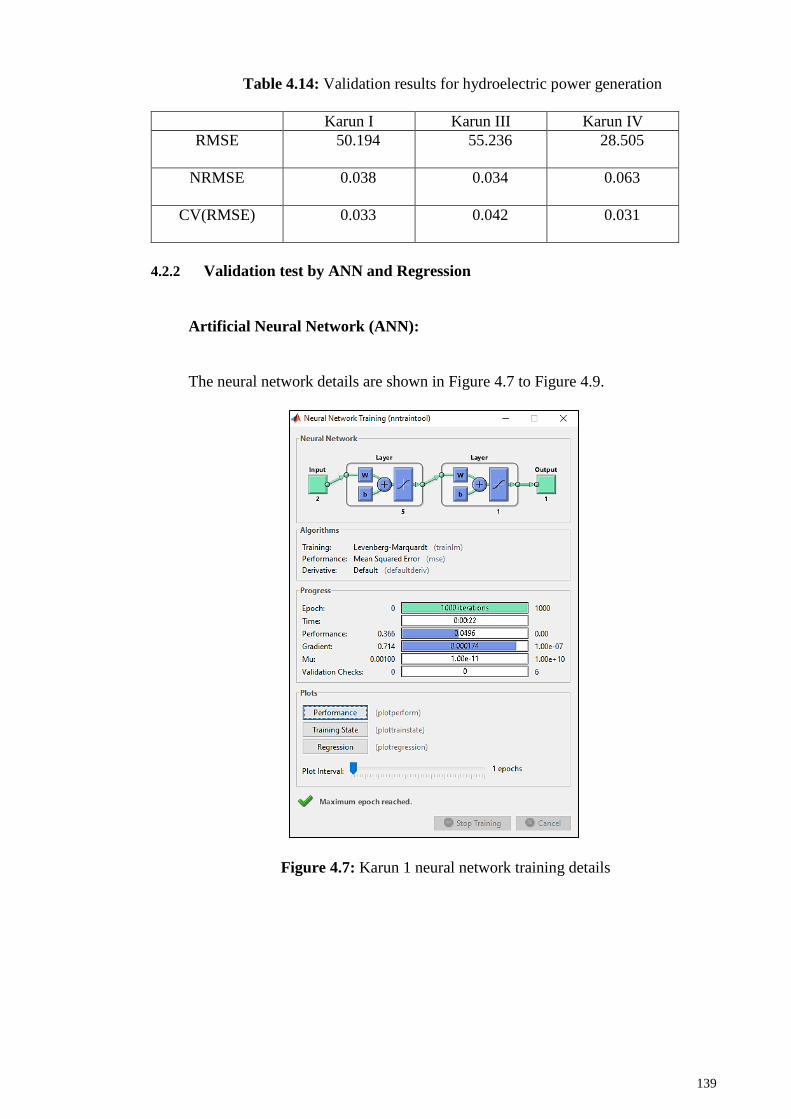
139

Table 4.14: Validation results for hydroelectric power generation


RMSE 50.194 55.236 28.505

NRMSE 0.038 0.034 0.063

CV(RMSE) 0.033 0.042 0.031

4.2.2 Validation test by ANN and Regression

Artificial Neural Network (ANN):

The neural network details are shown in Figure 4.7 to Figure 4.9.

Figure 4.7: Karun 1 neural network training details

140



141

The results of the Mean Squared Error on the training data have been demonstrated in the

Figure 4.10 to Figure 4.12.

MSE for train data in Karun 1 MSE for test data in Karun 1

Comparison of predicted and actual data in

train data for Karun I

Comparison of predicted and actual data

in test data for Karun I

Best training performance at 1000 epoch in

Karun I

Output-Target diagram for Karun I

result

Figure 4.10: MSE train and test for Karun I

142

MSE for train data in Karun III MSE for test data in Karun III


in train data for Karun III


in test data for Karun III

Best training performance at 1000 epoch

in Karun III

Output-Target diagram for Karun III

results

Figure 4.11: MSE train and test for Karun III

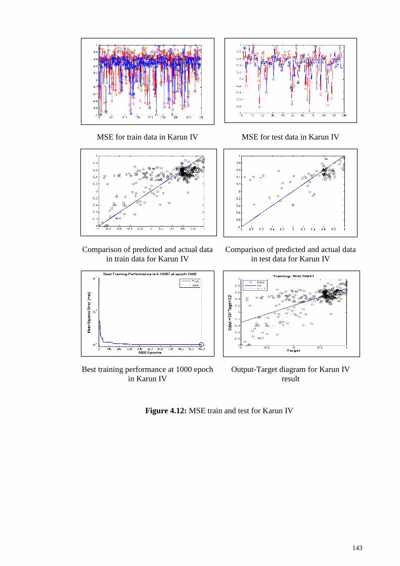
143

MSE for train data in Karun IV MSE for test data in Karun IV


in train data for Karun IV


in test data for Karun IV

Best training performance at 1000 epoch

in Karun IV

Output-Target diagram for Karun IV

result

Figure 4.12: MSE train and test for Karun IV

144

Table 4.15: Summary of MSE results

K1 K3 K4

MSE train 0.0496 0.0442 0.1037

MSE test 0.0688 0.0551 0.119

Regression Analysis Results

The t-test is one of the simplest and most common tests that are used for main

comparison. The full name of this test is Student's t-test.

The P value indicates the probable level that the hypothesis under testing (the null

hypothesis) is true. Therefore, if the p-value is 0.05, the probability of being true null

hypothesis is 0.05. Since in most cases the null hypothesis is tested, we want a lower level

of P to reject the null hypothesis. In the form of short, small amounts of p (p less than

0.05 indicates difference and the equal to or greater amount than 0.05 indicates that there

is no difference. Obviously, the smaller to be obtained p, one can conclude with more

confidence.

Confidence Limits: confidence limits show the accuracy of the computed average.

Confidence limits indicate that if the re- sampling of the population is done, the possibility

that samples are put in calculated average rang are 95%.

R-value or correlation coefficient is another statistical tool to determine the type and

degree of relationship of a quantitative variable. Correlation coefficient shows the

intensity of the relationship and the type of relationship (direct or inverse). This

coefficient is between 1 to -1 and if there is no relationship between two variables, it will

equal to zero, a large amount of it also shows a strong correlation between the amounts.

Underneath relation shows the calculation of R2. As the amount of R2 closes to one,

it shows that estimated equation has more accuracy.

R2 = Sxy2

Sx2Sy

2 = 1-SSE

∑(yi−y)2

(4.1)

145

The value of R2 is in fact a measure of how well the fitted regression line of the sample

is measured. Small amounts show that the model does not comply with the data. The

value of R2 is calculated as follows:

R2 = )1- Residual SS

Total SS ( =

Regress SS

Totall SS (4.2)

Adjusted R Squared has attempted to correct R square to reflect the highest rate of

adaption of in the population. The coefficient of determination was used to determine

which model is better:

AdjR2=1-(Total df

Residual df)(

Residual SS

Totall SS) (4.3)

Standard Error is a measure that shows how much the estimated average obtained is

accurate. So, if the SE is smaller, better estimation of population has been taking place

and vice versa. SE also is known as the standard deviation of the mean.

SE = SD

√n (4.4)

Table 4.16: Summary of regression statistics output


Multiple R 0.961904297 0.964227 0.984011

R Square 0.925259877 0.929733 0.968277

Adjusted R Square 0.92306653 0.927549 0.966171

Standard Error 80.29878012 63.96084 23.01699

Observations 492 492 492

The analysis of variance or ANOVA table checks the acceptance of the statistic. The

regression line shows information about a change in the model. Residual line also shows

the information about the change that is not intended for the model. In other words, the

residual of a product is equal to the observed the error term for the product. Total output

also shows the total data related to regression and residual.

(a) The number of independent observations minus the number of estimated

parameters is called the degree of freedom -regression. In other words, the degree of

146

freedom -regression- is a dimensional unknown volume (complete model) minus the

given volume (bound model).

(b) The Sum of square (SS) is composed of two sources of variance. In particular, it

is obtained from the sum of the SSregression and the SSresidual. It shows total variability

in the scores of the predicted variable Y.

∑(Y − Y) 2=∑(Y′ − Y) 2+∑(Y − Y′)2 (4.5)

(a) RegressionMS=(RegressionSS)/(Regressiondf) (4.6)

(b) F ratio is a number, which is obtained from dividing the average of Timar squares

by Residuals mean.

(c) Based on the F probability distribution, If the Significance F is not less than 0.1

(10%) one does not have a meaningful correlation (Wilcox, 2010).

Table 4.17: ANOVA results for Karun I

df SS MS F Significance F

Regression 2 39113249.36 19556624.68 3033.02511 2.4165E-276

Residual 490 3159468.104 6447.89409

Total 492 42272717.46

Table 4.18: ANOVA results for Karun III


Regression 2 26523584.09 13261792.04 3241.708444 6.742E-283

Residual 490 2004584.377 4090.988524

Total 492 28528168.46

Table 4.19: ANOVA results for Karun IV


Regression 2 7923455.161 3961727.58 7478.032886 0

Residual 490 259593.2037 529.7820484

Total 492 8183048.364

Results of inputs specifications and coefficients of the regression equation for

Karun reservoirs are presented in the following tables (Table 4.20 to Table 4.22):

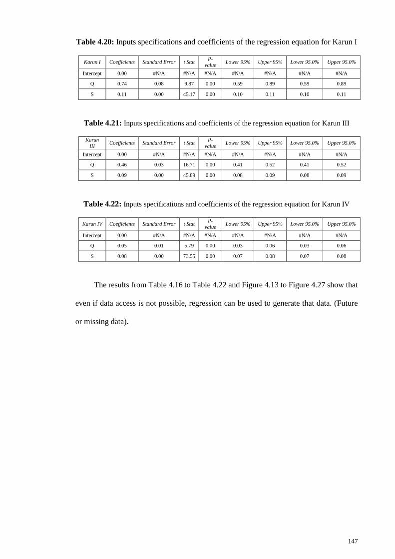
147

Table 4.20: Inputs specifications and coefficients of the regression equation for Karun I

Karun I Coefficients Standard Error t Stat P-

value Lower 95% Upper 95% Lower 95.0% Upper 95.0%

Intercept 0.00 #N/A #N/A #N/A #N/A #N/A #N/A #N/A

Q 0.74 0.08 9.87 0.00 0.59 0.89 0.59 0.89

S 0.11 0.00 45.17 0.00 0.10 0.11 0.10 0.11

Table 4.21: Inputs specifications and coefficients of the regression equation for Karun III

Karun

III Coefficients Standard Error t Stat

P-



Q 0.46 0.03 16.71 0.00 0.41 0.52 0.41 0.52

S 0.09 0.00 45.89 0.00 0.08 0.09 0.08 0.09

Table 4.22: Inputs specifications and coefficients of the regression equation for Karun IV

Karun IV Coefficients Standard Error t Stat P-



Q 0.05 0.01 5.79 0.00 0.03 0.06 0.03 0.06

S 0.08 0.00 73.55 0.00 0.07 0.08 0.07 0.08

The results from Table 4.16 to Table 4.22 and Figure 4.13 to Figure 4.27 show that

even if data access is not possible, regression can be used to generate that data. (Future

or missing data).

148

Figure 4.13: Q Residual Plot Karun I Figure 4.14: S Residual Plot Karun I

Figure 4.15: Q Line Fit Plot Karun I Figure 4.16: S Line Fite Plot Karun I

Figure 4.17: Normal Probability Plot Karun I

-300

-200

-100

0

100

200

300

0 100 200 300Re

sid

ual

s

Q-300

-200

-100

0

100

200

300

0 1000 2000 3000Re

sid

ual

s

S

0

200

400

600

0 100 200 300

R

Q

R Predicted R

0

200

400

600

0 1000 2000 3000

RS

R Predicted R

0

100

200

300

400

500

0 20 40 60 80 100 120

R

Sample Percentile

149

Figure 4.18: Q Residual Plot Karun III Figure 4.19: S Residual Plot Karun III

Figure 4.20: Q Line Fit Plot Karun III Figure 4.21: S Line Fite Plot Karun III

Figure 4.22: Normal Probability Plot Karun III

-200

-100

0

100

200

300

0 200 400 600 800

Re

sid

ual

s

Q-200

-100

0

100

200

300

0 1000 2000 3000

Re

sid

ual

s

S

0

200

400

600

0 200 400 600 800

R

Q

R Predicted R

0

200

400

600

0 1000 2000 3000

RS

R Predicted R

0

50

100

150

200

250

300

350

400

450

0 20 40 60 80 100 120

R

Sample Percentile

150

Figure 4.23: Q Residual Plot Karun IV Figure 4.24: S Residual Plot Karun IV

Figure 4.25: Q Line Fit Plot Karun IV Figure 4.26: S Fite Plot Karun IV

Figure 4.27: Normal Probability Plot Karun IV

-80

-60

-40

-20

0

20

40

60

80

0 500 1000 1500Re

sid

ual

s

Q-100

-50

0

50

100

0 500 1000 1500 2000Re

sid

ual

s

S

0

50

100

150

200

0 500 1000 1500

R

Q

R Predicted R

0

50

100

150

200

0 500 1000 1500 2000

RS

R Predicted R

0

20

40

60

80

100

120

140

160

0 20 40 60 80 100 120

R

Sample Percentile

151

4.3 Reservoir Storage

4.3.1 Calibration test by Linear Programming (LINGO)

Figure 4.28: Results of optimal storage for Karun I reservoir

152

Figure 4.29: Results of optimal storage for Karun III reservoir

153

Figure 4.30: Results of optimal storage for Karun IV reservoir

154

Table 4.23: Validation results for optimal reservoir storage


RMSE (MCM) 37.231 24.222 11.850

NRMSE 0.037 0.024 0.022

CV(RMSE) 0.017 0.012 0.007

4.3.2 Validation test by compared to the wet situation

Following the mentioned description in the introduction of model validation

method for reservoirs storage (compared to the wet situation section), we perform the

following steps. For this purpose, at first, we should provide time series inflow for

reservoirs to find out wet and dry years. A part of the inflow of the Karun reservoirs is

shown in Table 4.24 to Table 4.26 respectively in MCM. Also a histogram of Karun I, III

and IV reservoirs inflow for 41 years is shown in the Figure 4.31.

Table 4.24: Time series of Karun I reservoir inflow

Karun I Oct Nov Dec Jan Feb Mar Apr May Jun Jul Aug Sep

1970 31.54 33.28 36.00 38.88 53.36 110.43 103.50 46.34 36.15 32.44 28.61 30.92

1971 30.75 32.85 30.06 40.97 48.70 87.30 97.45 65.29 52.61 42.57 23.92 24.83

1972 32.17 35.20 54.44 48.34 57.76 78.74 105.82 36.51 24.69 22.71 33.71 34.96

...

2008 51.80 46.40 63.90 46.20 56.50 73.40 58.20 10.10 18.60 11.10 21.10 21.40

2009 26.10 29.10 177.30 28.00 77.30 57.30 84.00 47.80 16.10 30.10 44.20 22.60

2010 21.50 19.90 29.60 42.50 64.60 81.40 94.90 43.60 0.00 11.70 17.00 29.50

Table 4.25: Time series of Karun III reservoir inflow

Karun

III Oct Nov Dec Jan Feb Mar Apr May Jun Jul Aug Sep

1970 38.37 34.59 43.23 45.28 50.68 221.11 141.90 127.76 103.32 74.56 55.19 33.80

1971 37.26 30.58 36.19 62.22 51.29 211.98 273.74 290.78 198.30 126.82 89.61 59.31

1972 43.29 45.57 88.99 62.74 70.42 104.56 124.34 75.87 56.45 41.37 28.89 22.73

...

2008 75.38 73.97 64.12 59.96 70.11 79.49 98.83 78.32 49.15 29.76 21.83 16.71

2009 18.55 125.45 337.29 194.94 313.94 218.82 228.23 192.14 142.70 97.36 64.48 43.45

2010 40.86 45.26 50.69 71.99 118.44 313.96 406.86 280.93 158.96 95.45 68.26 45.80

155

Table 4.26: Time series of Karun IV reservoir inflow

Karun

IV Oct Nov Dec Jan Feb Mar Apr May Jun Jul Aug Sep

1970 64.80 65.30 83.50 82.30 113.20 264.70 252.70 219.30 151.20 106.50 80.90 67.80

1971 64.30 56.50 63.90 96.80 92.80 280.20 391.00 414.30 245.70 166.50 111.50 90.20

1972 69.80 75.10 125.70 92.50 118.60 189.60 205.10 150.40 102.60 68.10 58.20 52.30

...

2009 62.60 229.90 492.30 200.80 236.50 236.00 287.80 305.00 206.30 125.30 98.20 91.20

2010 72.30 69.10 70.20 78.40 119.60 306.70 527.50 427.50 226.50 131.70 97.60 77.30

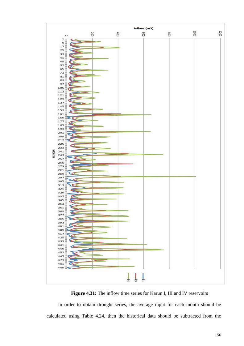
156

Figure 4.31: The inflow time series for Karun I, III and IV reservoirs

In order to obtain drought series, the average input for each month should be

calculated using Table 4.24, then the historical data should be subtracted from the

157

calculated averages (Figure 4.32 to Figure 4.34). The difference between the drought and

wet situation in Karun river dams are shown in Figure 4.35 to Figure 4.37.

Figure 4.32: The difference between the inflow and average inflow in Karun I

Figure 4.33: The difference between the inflow and average inflow in Karun III

-150

-100

-50

0

50

100

150

200

250

-7 43 93 143 193 243 293 343 393 443 493

Mo

nth

ly In

flo

w m

inu

s it

s av

era

ge in

flo

w (

m3

)

Months

Q minus Q ave

Q k1 - Q ave K1

-300

-200

-100

0

100

200

300

400

500

600

-7 43 93 143 193 243 293 343 393 443 493

Mo

nth

ly In

flo

w m

inu

s it

s av

era

ge in

flo

w (

m3

)

Months

Q minus Q ave

Q k3 - Q ave K3

158

Figure 4.34: The difference between the inflow and average inflow in Karun IV

-300

-200

-100

0

100

200

300

400

500

600

700

-7 93 193 293 393 493

Mo

nth

ly In

flo

w m

inu

s it

s av

era

ge in

flo

w (

m3

)

Months

Q minus Q ave

Q k4 - Q ave K4

159

Figure 4.35: The difference between the drought and wet situation in Karun 1 dam

160

Figure 4.36: The difference between the drought and wet situation in Karun III dam

161

Figure 4.37: The difference between the drought and wet situation in Karun IV dam

Table 4.27 shows a drought year with the most severity year of historical data.

Figure 4.38 shows the graph that belongs to this period.

162

Table 4.27: The difference between the average inflow and inflow in during the

drought condition (MCM) for Karun IV

Month Oct Nov Dec Jan

Fe

b Mar Apr May Jun Jul Aug Sep

Inflow 0.7 1.8 5 2.2

1.

9 1.7 5.9 1.4 2.2 1 2.1 0.9

Monthly average inflow 3.4 4.6 6.1 7.6

7.

9

10.

3

12.

5

12.

4 9.4 5.8 4.8 3.4

Inflow minus average

inflow

-

2.7

-

2.8

-

1.1

-

5.4 -6

-

8.6

-

6.6 -11

-

7.2

-

4.8

-

2.7

-

2.5

This means that, we consider this year as the base year for finding maximum storage

in drought period and similarly, we can do this for the wettest year to achieve the lowest

level of reservoir storage.

Figure 4.38: The difference between the average inflow and inflow in during the

drought condition (MCM) for Karun IV

The next step is to find the maximum storage of the reservoir, then a linear model

which is modelled in LINGO is used to calculate the maximum volume of the reservoir.

The gained values can validate the obtained results

Maximum Storage in drought period:

In this model the maximum amount of outflow is obtained for constant volume of

the reservoir ((4.7).

Minimize Z = C (4.7)

163

Subject to (4.8)

St+1 = St + it – qt – wt (4.9)

St ≤K (constant reservoir volume) (4.10)

St ≥ S1 (4.11)

Where, C is the reservoir capacity, St Storage of the month t, it inflow in month t,

wt the amount of overflow in month t and q is the constant monthly need of downstream.

The coding of the written model is in appendix F:

Table 4.28: The details of Karun reservoirs storages

Α Karun IV Karun III Karun I

Reservoir Storage 2192 2970 2993

Dead Storage 1097 1250 1864

Storage Area 29.23 48.2 54.8

Dead Storage Area 19.55 27.38 38.57

Modelling the evaporation losses in Karun reservoirs:

In order to calculate the amount of evaporation, the reservoir surface must be

calculated. The reservoir surface is a function of its volume (Figure 4.39).The specific of

this curve is convexity.

Figure 4.39: Evaporation relationship with the area and volume of reservoir (Loucks,

Stedinger, & Haith, 1981)

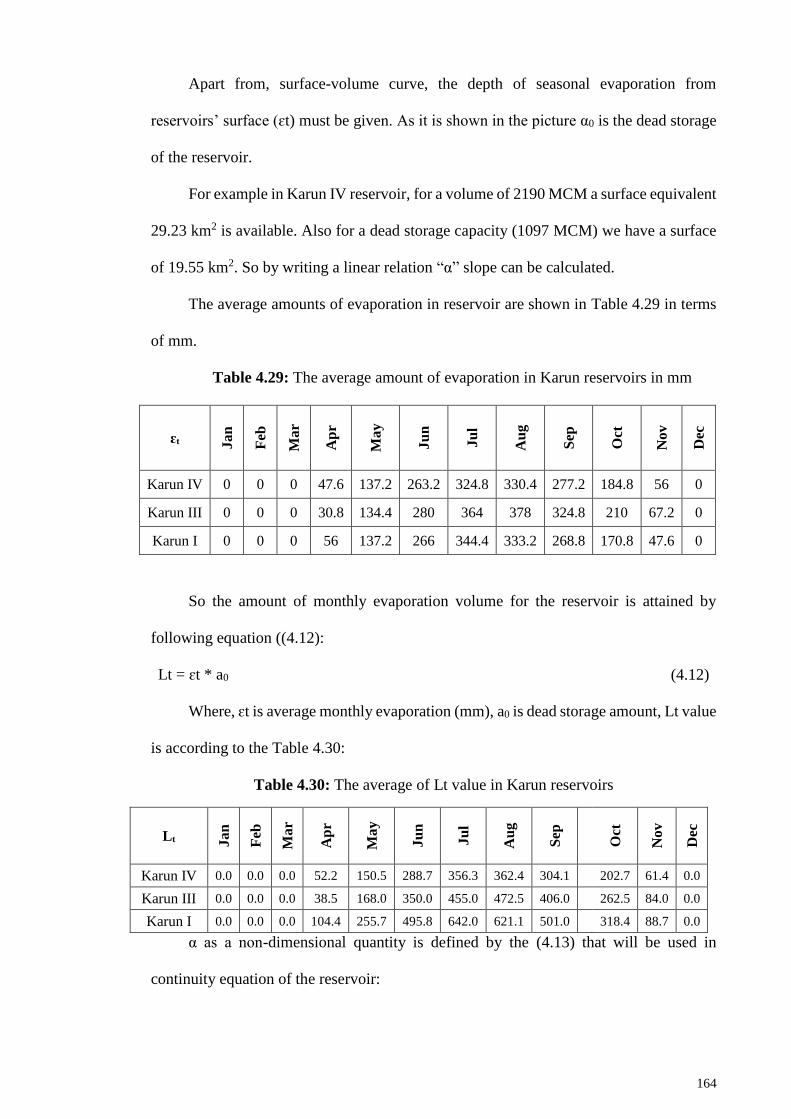
164

Apart from, surface-volume curve, the depth of seasonal evaporation from

reservoirs’ surface (ɛt) must be given. As it is shown in the picture α0 is the dead storage

of the reservoir.

For example in Karun IV reservoir, for a volume of 2190 MCM a surface equivalent

29.23 km2 is available. Also for a dead storage capacity (1097 MCM) we have a surface

of 19.55 km2. So by writing a linear relation “α” slope can be calculated.

The average amounts of evaporation in reservoir are shown in Table 4.29 in terms

of mm.

Table 4.29: The average amount of evaporation in Karun reservoirs in mm

ɛt Ja

n

Feb

Ma

r

Ap

r

Ma

y

Ju

n

Ju

l

Au

g

Sep

Oct

Nov

Dec

Karun IV 0 0 0 47.6 137.2 263.2 324.8 330.4 277.2 184.8 56 0

Karun III 0 0 0 30.8 134.4 280 364 378 324.8 210 67.2 0

Karun I 0 0 0 56 137.2 266 344.4 333.2 268.8 170.8 47.6 0

So the amount of monthly evaporation volume for the reservoir is attained by

following equation ((4.12):

Lt = ɛt * a0 (4.12)

Where, ɛt is average monthly evaporation (mm), a0 is dead storage amount, Lt value

is according to the Table 4.30:

Table 4.30: The average of Lt value in Karun reservoirs

Lt Ja

n

Feb

Ma

r

Ap

r

Ma

y

Ju

n

Ju

l

Au

g

Sep

Oct

No

v

Dec

Karun IV 0.0 0.0 0.0 52.2 150.5 288.7 356.3 362.4 304.1 202.7 61.4 0.0

Karun III 0.0 0.0 0.0 38.5 168.0 350.0 455.0 472.5 406.0 262.5 84.0 0.0

Karun I 0.0 0.0 0.0 104.4 255.7 495.8 642.0 621.1 501.0 318.4 88.7 0.0

α as a non-dimensional quantity is defined by the (4.13) that will be used in

continuity equation of the reservoir:

165

at = 𝛼ɛ𝑡

2 (4.13)

Table 4.31: The average of “at” value in Karun reservoirs

at Ja

n

Feb

Ma

r

Ap

r

Ma

y

Ju

n

Ju

l

Au

g

Sep

Oct

No

v

Dec

Karun IV 0 0 0 0.0210 0.0606 0.1163 0.1436 0.1460 0.1225 0.0817 0.0248 0

Karun III 0 0 0 0.0186 0.0813 0.1695 0.2203 0.2288 0.1966 0.1271 0.0407 0

Karun I 0 0 0 0.0403 0.0986 0.1912 0.2475 0.2395 0.1932 0.1228 0.0342 0

Noting the all mentioned above, the optimization model can be defined as follows

((4.14) to ((4.18):

Maximize Z = q (4.14)

Subject to (4.15)

(1+at)St+1 = (1-at)St + it – q – wt - Lt (4.16)

St ≤C (4.17)

St ≥ S1 (4.18)

The Lingo Coding is in the Appendix F.

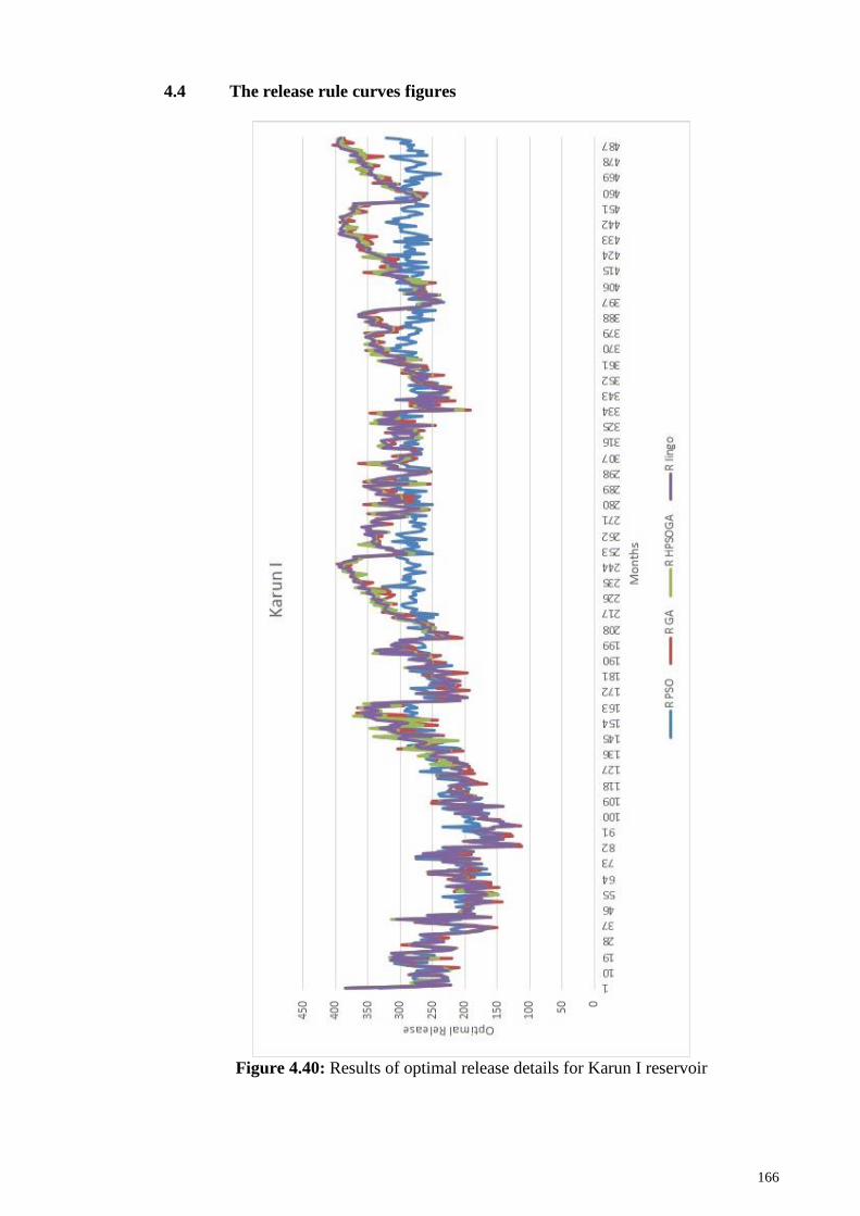
166

4.4 The release rule curves figures

Figure 4.40: Results of optimal release details for Karun I reservoir

167

Figure 4.41: Results of optimal release details for Karun III reservoir

168

Figure 4.42: Results of optimal release details for Karun IV reservoir

169

Table 4.32: Validation results for optimal release amount


RMSE (MCM) 10.048 9.959 4.139

NRMSE 0.036 0.0314 0.057

CV(RMSE) 0.035 0.043 0.033

4.5 Optimal Cropping Pattern

The optimization problem was solved using linear programming method and

evolutionary algorithm in Excel Solver. The results of both methods were completely

coincided. The details of the evolutionary algorithm solver engine are shown in

Table 4.35. Table 4.33 shows the optimal dedicated amount of land to the cropping pattern

of the mentioned seventeen agricultural products in the possession of six MCM water.

The objective function is the ultimate value of optimal cultivation pattern, which its value

obtained by sum of the multiplying the value per hectare (Toman) in the amount of

optimal allocated acres (ha). The optimal objective value in this problem for both methods

(LP and Evolutionary Algorithm) was exactly same and it is equal to 5,820,787,814

Toman.

Table 4.33: The optimal area of agricultural land for production (hectares) (The

data in this table is calculated only for the problem constraints and conditions)

Final Value (ha) Final Value (ha)

Wheat 377 Sugar beet 30

Barley 185 Watermelon 40

Husks 40 Cucumber 40

Corn 20 Potato 40

Pea 57 Onions 40

Lentil 59 Tomatoes 40

Cotton 8 Canola 72

Beans 60 Rice 110

Soy spring 60

170

As shown in Table 4.34, in total, about 208.5 tons of phosphate fertilizer, 288.7 tons

of nitrogen fertilizer and 271 tons of potassium fertilizer are needed for these products.

Nitrogen, phosphate and potassium have the most consumption for all the products

respectively. Due to high demand the maximum amount of fertilizer belongs to wheat,

barley and rice respectively. As can be seen in Table 4.34, the lowest amount of the

required fertilizer belongs to cotton with the value of 3.8 tons. Table 4.47, shows the cost

estimation of fertilizer used in an optimal crop pattern.

Table 4.34: The amount of consumed fertilizer in acre in optimum cropping pattern

(Weight unit: Kg)

Phosphate

Fertilizer

Nitrate

fertilizer

Potash

fertilizer Other Total

Wheat 57072 87381 6886 3043 154381

Barley 28107 33213 1705 1603 64629

Husks 9948 15906 898 458 27210

Corn 2882 6628 383 139 10032

Pea 2727 2851 323 22 5924

Lentil 5240 5768 331 1 11024

Cotton 1614 2059 120 21 3813

Sugar beet 7374 8250 1361 697 17682

Watermelon 7471 7769 636 1833 17708

Cucumber 10170 16443 2234 2796 31642

Potato 10778 14455 2808 478 28518

Onions 9325 13311 1132 1142 24910

Tomatoes 9531 15177 636 1339 27492

Canola 13239 16248 1374 369 31230

Beans 8879 9676 588 311 19453

Soya bean 6401 9390 2676 171 18639

Rice 17766 24142 2994 369 45272

Sum 208522 288667 27088 14791 539560

As shown in Figure 4.43, the wheat has highest water consumption compared to

other agricultural products (1622429.91 m3). In fact, four agricultural products with high

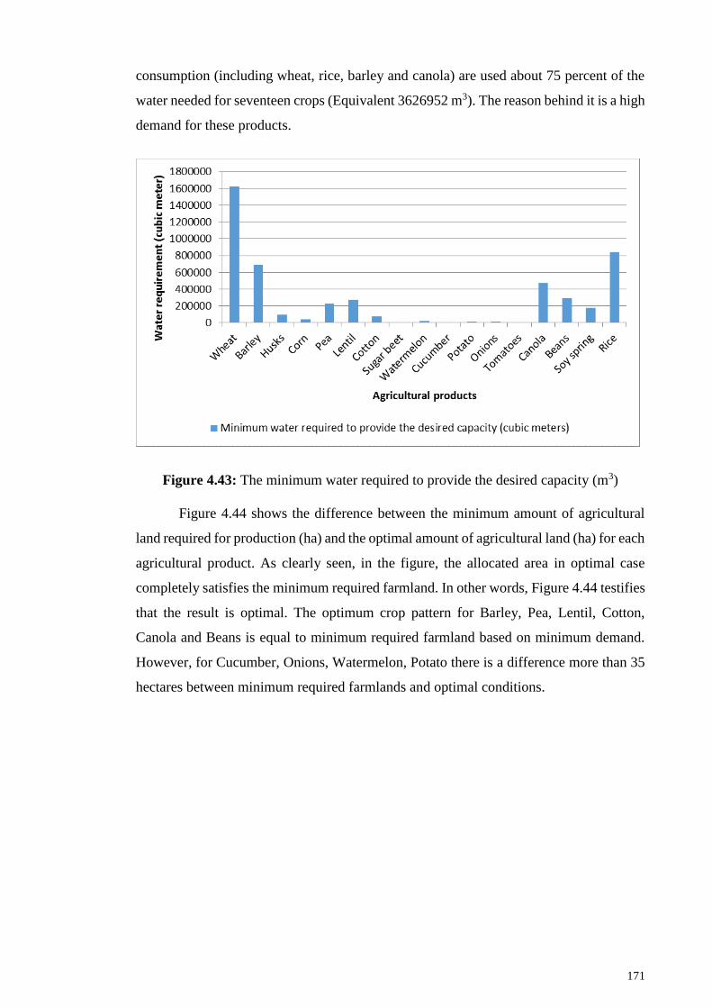
171

consumption (including wheat, rice, barley and canola) are used about 75 percent of the

water needed for seventeen crops (Equivalent 3626952 m3). The reason behind it is a high

demand for these products.

Figure 4.43: The minimum water required to provide the desired capacity (m3)

Figure 4.44 shows the difference between the minimum amount of agricultural

land required for production (ha) and the optimal amount of agricultural land (ha) for each

agricultural product. As clearly seen, in the figure, the allocated area in optimal case

completely satisfies the minimum required farmland. In other words, Figure 4.44 testifies

that the result is optimal. The optimum crop pattern for Barley, Pea, Lentil, Cotton,

Canola and Beans is equal to minimum required farmland based on minimum demand.

However, for Cucumber, Onions, Watermelon, Potato there is a difference more than 35

hectares between minimum required farmlands and optimal conditions.

172

Figure 4.44: The difference between the minimum amount of agricultural land and

the optimal amount of agricultural land (ha) for each agricultural product.

4.5.1 Calibration test by Linear Programming (Solver-Excel)

Table 4.35: Solver option for evolutionary algorithm

Evolutionary Engine:

40.375 Seconds Solution Time:

618 Sub problems:

0.000001 Precision

0.0001 Convergence

0.075 Mutation Rate

30 sec Time w/o Improve

1%, Integer Tolerance

173

4.5.2 Validation test by sensitivity analysis:

Table 4.36: The optimal area of agricultural land for production (hectares) and

sensitivity report of linear programming

Final

Value (ha) Reduced Cost

Objective

Coefficient

Allowable

Increase

Allowable

Decrease

Wheat 376.65 0 2808750 945557.6555 162494.4219

Barley 184.50 -300171.7742 2113800 300171.7742 1E+30

Husks 40.00 910698.3871 3615900 1E+30 910698.3871

Corn 20.00 2281102.258 5555820 1E+30 2281102.258

Pea 57.14 -554879.0323 1995000 554879.0323 1E+30

Lentil 58.58 -606431.4516 2390000 606431.4516 1E+30

Cotton 8.44 -716345.1613 5211800 716345.1613 1E+30

Sugar beet 30.00 5775994.355 8824200 1E+30 5775994.355

Watermelon 40.00 6568202.097 10354190 1E+30 6568202.097

Cucumber 40.00 3384725.806 5844000 1E+30 3384725.806

Potato 40.00 6788083.065 8710200 1E+30 6788083.065

Onions 40.00 4503286.29 7435000 1E+30 4503286.29

Tomatoes 40.00 6469357.258 7537200 1E+30 6469357.258

Canola 72.15 -314799.1935 3950100 314799.1935 1E+30

Beans 59.88 -184584.6774 3006000 184584.6774 1E+30

Soy spring 60.00 1885588.71 3969500 1E+30 1885588.71

Rice 110.00 5664892.742 11418300 1E+30 5664892.742

174

4.6 Accuracy of optimization algorithms (PSO, GA and HPSOGA)

As discussed in the methodology section, Particle Swarm Optimization (PSO),

Genetic Algorithms (GA) and the hybrid model of the two models (HPSOGA) are used

to obtain optimal release, optimal storage and the amount of hydro electric energy

produced for the three dams (Karun I, III, IV). In order to calibrate the results, a linear

programming method was used in the Lingo software. To compare the accuracy of the

results, three criteria were used for RMSE, NRMSD and CV (as mentioned in the

previous chapter).

4.6.1 Optimal hydroelectric generation

Karun 1 reservoir results: As seen in the Table 4.37, The RMSE errors obtained

from the PSO and GA method have the difference of 162.042 and 13.413 units compared

to HPSOGA algorithm result respectively. The calculated error rate according to the

NRMSD criteria, using the PSO and GA method has respectively 0.190 and 0.010 units

of error difference, compared to the combined method of the them (HPSOGA). The error

difference between the CV method for both PSO and GA algorithms are 0.119 and 0.009

units, respectively (Figure 4.45). These results confirm the better performance of the

HPSOGA algorithm compared to other two algorithms.



Karun I reservoir

Karun I Power (HPSOGA) Power(GA) Power(PSO)

RMSE 50/194 63/607 212/235

NRMSD 0/037 0/047 0/227

CV 0/033 0/043 0/152

175

Figure 4.45: Comparison of the NRMSD & CV errors for the optimization

algorithms (PSO, GA and HPSOGA) which are used to calculate the amount of

hydroelectric power generated in Karun I reservoir

Karun III reservoir results: Similarly, the RMSE error was compared to PSO and

GA optimization methods using HPSOGA algorithm (Table 4.38). This comparison

showed a difference of 163,993 and 19,63 of the mentioned methods compared to the

HPSOGA combination method. The NRMSD results showed 0.098 less precision for the

PSO method, and showed 0.011 less accuracy for GA method. Moreover, the CV results

for both PSO and GA showed 0.140 and 0.017 units of error compared to HPSOGA,

respectively (Figure 4.46).



Karun III reservoir

Karun III Power (HPSOGA) Power (GA) Power (PSO)

RMSE 55/236 74/868 219/229

NRMSD 0/033 0/044 0/131

CV 0/042 0/058 0/182

176



hydroelectric power generated in Karun III reservoir

Karun IV reservoir results: The above process was similar to Karun IV dam. The

RMSE error rate of the PSO and GA optimization methods compared to the HPSOGA

hybrid optimization method indicate an error difference of 167.733 and 7.954,

respectively (Table 4.39). The difference in error rate generated by the NRMSD for both

PSO and GA methods is 0.124 and 0.006, respectively, compared to HPSOGA algorithm.

The last criterion or CV, also fully reflects the greater error of the PSO method (equivalent

to 0.109), and then the GA algorithm (or 0.05) compared to the HPSOGA (Figure 4.47).



Karun IV reservoir

Karun IV Power (HPSOGA) Power (GA) Power (PSO)

RMSE 50/194 58/147 214/926

NRMSD 0/038 0/044 0/162

CV 0/033 0/039 0/143

177



hydroelectric power generated in Karun IV reservoir

The results generally indicate the lower accuracy of PSO and GA compared to

HPSOGA. Meanwhile, the results of the Genetic Algorithm (GA) are far better than the

Particle Swarm Algorithm (PSO).

4.6.2 Optimal release

Karun I reservoir results: According to Table 4.40 The error rate from the RMSE

criteria for PSO and GA algorithms compared to HPSOGA shows that their performance

is 4.893 times and 1.525 times worse. The NRMSD benchmark also is 7.353 times and

1.438 times greater in error compared to the HPSOGA model. As expected the third

criteria (CV) also indicates the better performance of the Genetic Algorithm (GA)

compared to the Particle Swarm Algorithm (PSO). (The PSO method error is about 5.335

times more than HPSOGA and for GA algorithm error is 1.544 times more than HPSOGA

algorithm.)(Figure 4.48)

178


HPSOGA) which are used to calculate the amount of optimal release in Karun I reservoir

Karun I Release (HPSOGA) Release (GA) Release (PSO)

RMSE 10/048 15/327 49/162

NRMSD 0/036 0/052 0/268

CV 0/035 0/055 0/188


algorithms (PSO, GA and HPSOGA) which are used to calculate the amount of optimal

release in Karun I reservoir

Karun III reservoir results: According to the Table 4.41 by dividing the obtained

error from PSO and GA methods into HPSOGA results using the RMSE criteria is can

be seen that the PSO is 4.141 times and the GA is 2.794 times worse. Using the same

method but this time under NRMSD criteria, the error rate for PSO method is for 4.721

worse and for GA method is 2.819 worse than HPSOGA results. The CV criteria results

also fully support the above results (Figure 4.49).

179


HPSOGA) which are used to calculate the amount of optimal release in Karun III

reservoir

Karun III Release (HPSOGA) Release (GA) Release (PSO)

RMSE 9/959 27/820 41/237

NRMSD 0/030 0/085 0/142

CV 0/043 0/110 0/179



release in Karun III reservoir

Karun IV reservoir results: Similarly, the RMSE error ratio for PSO and GA

optimization methods compared to HPSOGA was 4.752 and 1.426, respectively

(Table 4.42). These results also indicate highest accuracy of HPSOGA, then GA and

eventually PSO (Figure 4.50).

180


HPSOGA) which are used to calculate the amount of optimal release in Karun IV

reservoir

Karun IV Release (HPSOGA) Release (GA) Release (PSO)

RMSE 10/048 14/329 47/747

NRMSD 0/036 0/052 0/173

CV 0/035 0/050 0/167



release in Karun IV reservoir

4.6.3 Optimal storage

Karun I reservoir results: The accuracy of the PSO results compared to HPSOGA

has a difference of approximately 275 units difference in RMSE, 0.311 in NRMSD and

0.119 units in CV (Table 4.43). It should be noted that the accuracy of GA results is far

better than PSO (Figure 4.51).

181


HPSOGA) which are used to calculate the amount of optimal storage in Karun I reservoir

Karun I Storage (HPSOGA) Storage (GA) Storage (PSO)

RMSE 37/231 44/275 312/129

NRMSD 0/037 0/043 0/348

CV 0/016 0/019 0/135



storage in Karun I reservoir

Karun III reservoir results: According to the Table 4.44 comparison of the

accuracy of the results indicates a better performance of the GA than the PSO. (About 7

times better in terms of criteria RMSE and CV and 8.2 times better in terms of criteria

NRMSD) (Figure 4.52)

182


HPSOGA) which are used to calculate the amount of optimal storage in Karun III

reservoir

Karun III Storage (HPSOGA) Storage (GA) Storage (PSO)

RMSE 24/222 33/669 271/936

NRMSD 0/024 0/033 0/244

CV 0/012 0/017 0/133



storage in Karun III reservoir

Karun IV reservoir results: In all the obtained results, i.e. release, optimum storage and

the produced energy, for all dams, the accuracy of HPSOGA was better than GA and GA

accuracy was remarkably better than PSO (

Table 4.45). However, exceptionally, the accuracy of the GA algorithm was

approximately 34% better than the HPSOGA algorithm for only the optimal storage

capacity at Karun IV Dam (Figure 4.53).

183


HPSOGA) which are used to calculate the amount of optimal storage in Karun IV

reservoir

Karun IV Storage (HPSOGA) Storage (GA) Storage(PSO)

RMSE 37/231 12/824 312/129

NRMSD 0/037 0/013 0/309

CV 0/016 0/006 0/137



storage in Karun IV reservoir

4.7 Predicting the Cost of agricultural products

After determining the optimal amount of agricultural land for these 17 agricultural

products per hectare (Table 4.33), the cost of land preparation, planting, crop processing

are easily calculated, by using the costs set by the Ministry of Agriculture in different

stages of farming (Table 3.13). Table 4.46 shows the breakdown cost for these 17 crops.

184

Table 4.46: The estimated cost of planting, maintenance and harvesting

Total

Cost

Farmland

Cost

Harvesting

Cost

Maintenance

Cost

Planting

Cost

Farmland

Preparation

Cost

Wheat 240544.2 73027.0 27228.8 67771.3 46101.0 26416.0

Barley 102704.8 26421.2 12793.4 31230.1 19093.5 13166.6

Husks 99711.8 26883.0 12392.7 28701.9 21136.0 10598.2

Corn 17515.7 5692.5 1738.3 6240.6 2300.8 1543.4

Pea 20667.9 4707.3 4583.1 5766.2 3288.9 2322.4

Lentil 36784.4 8011.9 9858.5 9776.5 5646.5 3491.0

Cotton 9767.5 1474.9 2104.7 4487.9 1044.0 656.1

Sugar beet 42557.8 6033.0 10358.0 17877.8 5983.7 2305.3

Watermelon 47632.3 7984.5 12447.4 13301.8 9262.4 4636.2

Cucumber 103530.1 13291.1 33046.4 29873.7 20865.8 6453.1

Potato 111293.4 14211.4 19136.6 25501.1 48560.8 3883.4

Onions 105382.4 14439.3 33913.2 33735.4 16906.6 6388.0

Tomatoes 118586.8 15512.3 47480.9 33382.9 17207.2 5003.5

Canola 54515.9 18350.5 5366.5 19052.2 6126.3 5620.4

Beans 71285.3 16433.9 13747.6 24337.8 11887.7 4878.3

Soya bean 43528.0 17170.8 5080.2 11832.5 4245.6 5198.9

Rice 276330.3 81065.6 40048.6 66200.2 60037.9 28978.1

185

Table 4.47: The cost estimation of consumed fertilizer in acre in optimum cropping

pattern (Currency unit: TOMAN)

Phosphate

Fertilizer

Nitrate

fertilizer

Potash

fertilizer Other

Wheat 29379 24859 22976 47458

Barley 13838 11070 11808 22140

Husks 4360 1720 3680 13960

Corn 1660 1460 1540 5720

Pea 4514 3543 3086 10228

Lentil 4686 4335 3163 87870

Cotton 675 549 532 5165

Sugar beet 2820 2190 1980 3840

Watermelon 3640 3000 3240 7360

Cucumber 3680 3160 3280 8200

Potato 3560 3240 2760 12640

Onions 3960 3760 2680 7400

Tomatoes 4080 3760 3240 9280

Canola 5988 4762 4834 24603

Beans 5569 4671 4731 9401

Soya bean 3720 2760 4020 94920

Rice 14960 11220 7810 20790

Sum 111089 90058 85359 390976

186

CHAPTER 5: CONCLUSION AND RECOMMENDATION

5.1 Introduction

Achieving optimal operation rules in multi-reservoir systems is an important topic

that has received lots of attention from water resource planners. It is obvious that, a slight

improvement in the performance of these systems will lead to noticeable economic

income.

There is not any comprehensive approach to solve all the optimization models,

efficiently. Therefore, we tend to model the economical and physical aspects of water

resources systems with one or more efficient optimization algorithms. Modelling the

optimal utilization system in the reservoirs is of important factors that should be

considered. Therefore, in this study, the following items were considered as much as

possible:

1. Models should be as simple as they were described by terms and be

understandable by non-specialists, those who have no scientific background.

2. If the model is developed in the real world, it should be adaptable enough to be

able to unify the rapid changes that may be experienced in the current or future world.

3. The model should include all aspects of the problem, not only some details of it.

4. Models should be user friendly as much as possible.

The best method for solving constrained optimization model depends on the

specified mathematical form of the objective function and equations. There is not any

comprehensive method for efficient solving of all the optimization models. Thus, every

mathematical programming model in its best way is only an approximate description of

the actual water resources system. The obtained answer is only optimized to the prepared

model not to the real problem.

The present study has used evolutionary algorithms and linear programming

techniques. Control curves in storage system show the optimum or the appropriate amount

187

of system's delivery water for the storage reservoir condition and input to the reservoir

during different months.

In this study, we aimed to maximize hydroelectric power production, water supply

for agricultural needs and control seasonal flooding by using multi-objective

programming, which has been modelled and optimized, regarding the operation of the set

of Karun reservoir dams, which are the main system of reservoir dams in Iran. From

evaluation of optimization time due to its high dimensions regarding the number of

limitations and decision variables in a 40-year period, it was identified that

implementation of the matrix structure and using evolutionary algorithms are appropriate

tools to optimize linear and nonlinear models with large dimensions. Then, computational

results were obtained by solving the model using different scenarios for combinations of

the objective functions. After reviewing these results, it was found that the impact of

hydroelectric power is quite impressive in the determination of the optimum solution in

comparison with the function of providing water demand. These results provide a useful

means to decide for the optimal amount of flow passing through the turbines, the rate of

water flowing and the amount of water supply for agricultural and industrial purposes in

the short term and long term planning for executives and decision-makers. (Heydari et

al., 2016).

This study has two new innovations for optimizing the reservoir operation:

Planning for present and future using regression analysis and artificial neural

networks (in situations of data insufficiency or data generation for the future)

Integrated and optimal resource management, from planning to operation.

(Connecting the optimizer model to optimal water allocation for agricultural land and

estimate the amount of agricultural products and predict the cost before implementation.

188

5.2 Conclusion

5.2.1 System release rule and reservoir balancing functions

In a real-world situation, release decisions are continuously being made. The operator

is continuously assessing the storage levels at every reservoir, estimating the current

inflow rates, forecasting future hydrological conditions and deciding if the current release

rates need to be revised.

The operating rules are used to compute the rate of release from each reservoir.

Knowing the total amount of water in storage in the system, the operator uses the release

rule of the current season to determine the rate of release from the system. Next, the

operator has to decide which reservoirs has to be used to meet the determined rate of

release. The balancing functions for the current season are used to compute the ideal

storage level for each reservoir given the current amount of water in storage in the system.

If the system storage is balanced according to the ideal storage levels, the operator should

release at the release rate specified by the release rule while attempting to maintain the

ideal balance. If the system storage is not perfectly in balance, the operator should release

at the release rate specified by the release rule and try to achieve the ideal balance as soon

as possible. The operator has some freedom on how to achieve the ideal storage balance,

but as a rule reservoirs with a storage level above their ideal level will release more than

reservoirs with storage levels below their ideal level. The decisions of the operator have

to take into consideration the physical limitations of the system structures and equipment,

and the short-term operational requirements such as water and energy demand schedules.

Note that the long-term operational requirements are being implicitly considered by the

operating rules.

Simulating this continuous decision process is not straightforward, since a simulation

model uses a discrete time-step. A key issue the model builder has to decide is whether

189

the inflow of the next immediate simulation period is considered available for use during

that period. In this case, the inflow is assumed known at the time of the decision, i.e. the

beginning of the period.

In real-world situations, although the operator does not know with certainty the future

inflows, he or she knows the past and current inflow rates and may have reliable short-

term forecasts of future inflows. The operator is continuously making release decisions

that are revised as soon as new information about the inflows becomes available. This

situation is better represented by assuming the inflow for the next immediate simulation

period is known at the time of the decision. Therefore, in this study, in addition to

conventional operational planning, Artificial Neural Networks and Regression Analysis

were used for future behaviors of the reservoir.

5.2.2 Cropping pattern

One of the most practical objectives of this study is to develop a mathematical

programming model for optimal allocation of resources in agricultural field in Khuzestan

region. For designing an optimal cropping pattern in an irrigation and drainage network

that has defined resources and restrictions, different methods are available for managers

and researchers.

The optimal use of natural and human resources is an important objective of economic

and social aspects that in this case, fundamental and sweeping changes in the structure of

agriculture, the extensive involvement of staff and favorable management factors of

production, are necessary to develop the agricultural sector in the country. In this

communication, design and adjusting the cropping pattern to determine the amount of

cultivated area and the right combination of products, is utmost important and should be

done in such way that in addition to the optimal use of existing capacities and access,

considering regional and national needs. Design cultivated and process are influenced by

190

many varied factors that are studied that force the designer pattern to collect a wealth of

data and information.

Performing appropriate cropping pattern guarantees food security, production

stability, reduction in the adverse effects of drought it is necessary to protect natural

resources and increase efficiency production factors. But, for performing appropriate

cropping pattern we require common intrinsic county planning, coordination and

cooperation of power ministries, agriculture and commercial institutions.

Design and adjustment of the cropping pattern is utmost important to determine the

amount of cultivated area and the right combination of products. It should be done in such

way that in addition to achieve the optimal use of existing capacities and access, regional

and national needs are being considered.

Cultivated design and process are influenced by many varied factors that force the

designer to collect a wealth of data and information. It is crucial to pay particular attention

to the projects’ effective operation to obtain the utmost benefits and satisfaction from all

the goals set earlier (Heydari et al., 2015).

In general, the results obtained from this study show that the farmers do not use the

available resources efficiently. Implementation of optimization models indicates that the

use of arable land in different seasons can lead to done in a better way. Therefore, if the

limits of the region, including water, reduced, there will be a possibility of increasing the

area under cultivation and profitability. The development of infrastructural services play

an immense role in reducing resource constraints, and optimal use of resources can be

effective to achieve the desired profitability of farming activities.

191

According to estimations of water’s shadow price, it can be stated with certainty that

water is the most limiting factor in the region's agriculture. Therefore increasing the

accessibility of farmers to water can be increased acreage and farmers' incomes.

If we consider several watershed areas, we can divide the watersheds to different

general arena based on water resources and raining rate .In each arena, the general policies

of reaching to an appropriate cropping pattern with the focus on water resources are

similar to each other (even in different climates), these arenas include:

Arena that has severe water restriction

At the present, policies based on indiscriminate consumption of underground water

resources are dominated; therefore, it is necessary that production policies are for optimal

consumption and high efficiency and non-reduction of production as much as possible.

For performing this policy the following methods should be considered:

1. Giving priority to fall plants for using annual fall, winter and spring rains.

2. Increasing the cultivation area in controlled environments such as

greenhouse, cultivation under plastic

3. In spring cultivation using plants that their growing period is short and

have more adaptation with rainfall distribution of the area.

4. Establishment of Conservation tillage systems

5. Establishment of pressurized irrigation lands, especially drip irrigation in

agricultural lands and garden

6. Reduction of water consumption and increasing economic efficiency and

preserving basic resources

192

7. Plants with low water needs and cultivation kinds of yielding precocious

plants

Arenas that have no water restriction

In these areas, agricultural operation policies should go toward maximum

utilization of land for production and the following methods are considered:

1- Moving toward multi-cultivation methods

2- Maximum utilization of water resources with the aim of keeping the

potential of production resources

3- Proper utilization of tail water of reservoirs that includes optimization of

cropping pattern and proper exploiting of production resources.

5.2.3 Hydropower generation

Since, the production of hydroelectric energy is a function of the reservoir volume and

release rate, the objective function for energy production is in contrast with the objective

function for agricultural and industrial needs and for flood control. Therefore, large

amounts of water cannot stored behind the dam exit from the turbines. On the other hand,

the increased volume of water stored behind the dam will increase the amount of energy

produced per month. Hydroelectric power production is the function of the height of the

water stored behind the dam and the volume of water passing through the turbine.

However, increasing the water release rate for hydroelectric power production is

relatively more effective than increasing the height of water stored behind the dam

because of the physical structure of reservoir dams and location of turbines. When the

volume of water stored behind the dam is close to its maximum and it is not possible to

drain the water from the tunnel, there will be an overflow throw out-lets. With the

193

increased volume of water passing through the turbines, the water level increases in the

tailwater. Increasing water height in the tailwater will decrease hydroelectric power

production. For this reason, it is not so often possible to release the water to the extent of

the water capacity of the tunnels. A comparison between the results of the evolutionary

algorithms optimization model and mathematical programming methods for

implementing the best scenario showed that there is a good match between them.

The results also showed that the volume of seasonal flooding increases solely in the

spring, and overflows through sub-outlets and the discharged water volume is very low

through these sub-outlets in the other months. The percentage of consumption needs of

an area is estimated at 35-40%, which has the lowest value of 26% in September and the

highest value of 56% in December. Hydroelectric energy is produced to the highest and

lowest level, in the months of June and January with a production value of 327242 (MWh)

and 160070 (MWh) energy, respectively (Heydari et al., 2016).

5.2.4 Flood control

In the catchments under study, generally high flow is observed in two distinct

periods, from November to February (winter) and from March to May (spring). Heavy

precipitation is responsible for winter floods, whereas the combined effects of rainfall and

snowmelt produce the spring floods.

194

5.3 Recommendation

5.3.1 Reservoir rule curves considerations

The majority of reservoir systems is still managed through fixed and pre-defined

operating rules that indicate with varying detail the actions to be taken by the system

operators as a function of small number of variables, such as the time of the year, state of

the system and hydrological conditions. These pre-defined rules are usually presented in

the form of charts or tables that are very easy to understand, and constitute a good working

tool for negotiations on reservoir systems operations. Since the operating rules are easily

readable, little modelling or scientific background is required to take part in the

discussion. In our view, this possibility for discussion and modification is the main reason

why the great majority of reservoir systems is still managed by these type of rules.

Simulation models are very useful at this stage of discussion and included in these models

to represent the actual operating decisions taken by the operator of the system being

simulated, and they can quickly be modified to meet suggestions that arise during the

discussions.

5.3.2 Cropping pattern suggestions

Suggestions for future studies

1. It is recommended to calculate the actual performance of the product and

the actual evaporation-transpiration more accurately by using a nonlinear programming

model and considering the soil moisture balance (at ten-day irrigation intervals obtained

from the local information) and also considering the dynamic aspects of root growth,

therefore the results would be more desirable.

2. It is suggested to link the provided model with the geographical

information system software (GIS) and add the zoning capabilities of cultivation pattern

195

to this model. This will cause to obtain the optimal cultivated area of each product from

the surface and underground water resources of the plain.

3. It is recommended to link the provided model with Modflow to be able to

carry out analyses related to the drop in the water table aquifer and accurately calculate

the changes in aquifer volume.

Suggestions for managers:

1. Developing the regional cultivation patterns based on reducing the use of scarce

water resources.

2. Using the water markets in order to change the process of utilizing water

resources.

3. Noticing the effects of government policies on local products because of the

exchange relationship between numerous objectives such as intervention in products’

market.

5.3.3 Suggestions for hydropower generation modelling

Suggestions for future studies

If researchers wish to continue research on the optimal production of hydroelectric

power, it is recommended to consider the following hydroelectric schemes parameters in

their model.

Parameters for Hydroelectric Schemes in desired model:

1. Year of commissioning (for existing or committed plant);

2. Earliest allowable year of commissioning (for candidate plant);

3. Normal life expectancy;

196

4. Plant displaced by this station;

5. Reservoir storage capacity (GWh of energy);

6. Number of generating units;

7. Nominal installed capacity of units (MW);

8. Station internal demand (% of installed capacity);

9. Loss in interconnector to the grid (%);

10. Minimum power output (MW);

11. Firm power and average power in each month of year (MW);

12. Firm energy and average energy in each month of year (GWh);

13. % available storage for each month of firm year and in average year (% of

live storage capacity);

14. station availability in each month (% time/capacity);

15. forced outage rate in each month (% of time);

16. minimum generation level (MW) in each month of year (to allow for

programmed releases for other water users);

17. fixed operating costs (currency unit per MW per annum);

18. variable operating costs (currency unit per MWh);

5.3.4 Suggestions for flood control

Flood control

We need flood frequency analysis to identify the flood magnitude for every return

period. Hence, a thorough flood frequency analysis has to be carried out for the upper and

intermediate catchment. The initial condition of the reservoirs and flood hydrograph

combination of the catchment determine how critical the situation is. So, the calculated

hydrograph in upstream indicates the maximum possible flood based on the river system

features. The hydrodynamic simulation is needed to obtain flood inundation depth in the

197

flood plain. To achieve this, the HEC—RAS model (or any relevant models) can be used

by applying available data from Dez and Karun rivers.

A very important aspect of flood studies is estimating the flood damage in inundated

regions. In order to figure out an accurate damage amount, gathering historical data of

damage and having the result of a flood damage survey are necessary.

The results obtained from the survey and the maps are applied to build a GIS

database. In some conditions and mitigation plan alternatives, the hydraulic model will

run to forecast discharges as well as water levels for various return periods of flood the

damage in different return periods are evaluated.

To analyse the cost/benefit of various mitigation alternatives HEC-FDA software

can be used. To calculate the annual benefits of a specific mitigation alternative a risk-

based damage analysis is carried out. Moreover, in order to opt the most desirable

alternative an economic assessment will be done based on cost-benefit analysis.

198

REFERENCES

Afshar, A., Haddad, O. B., Mariño, M. A., & Adams, B. (2007). Honey-bee mating

optimization (HBMO) algorithm for optimal reservoir operation. Journal of the

Franklin Institute, 344(5), 452-462.

Afshar, M. (2013). Extension of the constrained particle swarm optimization algorithm

to optimal operation of multi-reservoirs system. International Journal of Electrical

Power & Energy Systems, 51, 71-81.

Afshar, M., Azizipour, M., Oghbaeea, B., & Kim, J. H. (2017). Exploring the Efficiency

of Harmony Search Algorithm for Hydropower Operation of Multi-reservoir

Systems: A Hybrid Cellular Automat-Harmony Search Approach. Paper

presented at the International Conference on Harmony Search Algorithm.

Afshar, M. H., & Shahidi, M. (2009). Optimal solution of large-scale reservoir-operation

problems: Cellular-automata versus heuristic-search methods. Engineering

Optimization, 41(3), 275-293. doi:10.1080/03052150802441273

Ahmed, J. A., & Sarma, A. K. (2005). Genetic algorithm for optimal operating policy of

a multipurpose reservoir. Water Resources Management, 19(2), 145-161.

Alabdulkader, A. M., Al-Amoud, A. I., & Awad, F. S. (2012). Optimization of the

cropping pattern in Saudi Arabia using a mathematical programming sector

model. Agricultural Economics (Zemedelská Ekonomika), 58(2), 56-60.

Ali, R., Awan, T., Ahmad, M., Saleem, U., & Akhtar, M. (2012). Diversification of rice-

based cropping systems to improve soil fertility, sustainable productivity and

economics. Journal of Animal and Plant Sciences, 22(1), 108-112.

Angeline, P. J. (1998). Evolutionary optimization versus particle swarm optimization:

Philosophy and performance differences. Paper presented at the Evolutionary

Programming VII.

Ashofteh, P.-S., Haddad, O. B., & Loáiciga, H. A. (2015). Evaluation of climatic-change

impacts on multiobjective reservoir operation with multiobjective genetic

programming. Journal of Water Resources Planning and Management, 141(11),

04015030.

Baltar, A. M., & Fontane, D. G. (2008). Use of multiobjective particle swarm

optimization in water resources management. Journal of water resources planning

and management, 134(3), 257-265.

Baltar, A. M., & Fontane, D. G. (2008). Use of multiobjective particle swarm

optimization in water resources management. Journal of Water Resources

Planning and Management, 134, 257.

Barakade, A., Tonape, L., & Lokhande, T. (2011). Agricultural land use pattern in Satara

District of Maharashtra. Research Analysis and Evaluation, 2(17), 12-15.

Bayat, P. (1999). Determine the optimal cropping pattern with conjunctive use of surface

and ground water resources: A case study Borazjan plain (In Persian). (MSc

thesis), University of Shiraz.

199

Bodruzzaman, M., Meisner, C., Sadat, M., & Hossain, M. I. (2010). Long-term effects of

applied organic manures and inorganic fertilizers on yield and soil fertility in a

wheat-rice cropping pattern. Paper presented at the 19th World Congress of Soil

Science, Soil Solutions for a Changing World.

Boustani, F., & Mohammadi, H. (2010). Determination of optimal cropping pattern due

to water deficit: A case study in the south of Iran. American-Eurasian Journal of

Agricultural and Environmental Sciences, 7, 591-595.

Brooke, A., Kendrick, D., Meeraus, A., Raman, R., & Rasenthal, R. (1998). A user’s

guide, GAMS software. GAMS Development Corporation.

Cai, X., McKinney, D. C., & Lasdon, L. S. (2001). Solving nonlinear water management

models using a combined genetic algorithm and linear programming approach.

Advances in Water Resources, 24(6), 667-676.

Chang, F.-J., Chen, L., & Chang, L.-C. (2005). Optimizing the reservoir operating rule

curves by genetic algorithms. Hydrological processes, 19(11), 2277-2289.

Chang, L. C., & Chang, F. J. (2001). Intelligent control for modelling of real‐ time

reservoir operation. Hydrological processes, 15(9), 1621-1634.

Cheng, C.-t., Liao, S.-l., Tang, Z.-T., & Zhao, M.-y. (2009). Comparison of particle

swarm optimization and dynamic programming for large scale hydro unit load

dispatch. Energy Conversion and Management, 50(12), 3007-3014.

Cheng, C.-T., Wang, W.-C., Xu, D.-M., & Chau, K. (2008). Optimizing hydropower

reservoir operation using hybrid genetic algorithm and chaos. Water Resources

Management, 22(7), 895-909.

Cheng, C., Wang, S., Chau, K.-W., & Wu, X. (2014). Parallel discrete differential

dynamic programming for multireservoir operation. Environmental modelling &

software, 57, 152-164.

Christensen, V. G., Jian, X., Ziegler, A. C., & Demonstration, E. B. G.-w. R. (2000).

Regression analysis and real-time water-quality monitoring to estimate

constituent concentrations, loads, and yields in the Little Arkansas River, south-

central Kansas, 1995-99: US Department of the Interior, US Geological Survey.

Cieniawski, S. E., Eheart, J. W., & Ranjithan, S. (1995). Using genetic algorithms to solve

a multiobjective groundwater monitoring problem. Water Resources Research,

31(2), 399-409.

Clerc, M. (1999). The swarm and the queen: towards a deterministic and adaptive particle

swarm optimization. Paper presented at the Evolutionary Computation, 1999.

CEC 99. Proceedings of the 1999 Congress on.

Dariane, A., & Moradi, A. M. (2010). Application of ant-colony based algorithms to

multi-reservoir water resources problems. J. Water Wastewater, 76(4), 81-91.

200

Dariane, A. B., & Momtahen, S. (2009). Optimization of multireservoir systems operation

using modified direct search genetic algorithm. Journal of Water Resources

Planning and Management, 135(3), 141-148.

Deb, K., Pratap, A., Agarwal, S., & Meyarivan, T. (2002). A fast and elitist multiobjective

genetic algorithm: NSGA-II. Evolutionary Computation, IEEE Transactions on,

6(2), 182-197.

Del Castillo, E., Montgomery, D. C., & McCarville, D. R. (1996). Modified desirability

functions for multiple response optimization. Journal of quality technology, 28,

337-345.

Doppler, W., Salman, A. Z., Al-Karablieh, E. K., & Wolff, H.-P. (2002). The impact of

water price strategies on the allocation of irrigation water: the case of the Jordan

Valley. Agricultural Water Management, 55(3), 171-182.

Eberhart, R. C., & Shi, Y. (1998). Comparison between genetic algorithms and particle

swarm optimization. Paper presented at the Evolutionary Programming VII.

Eberhart, R. C., & Shi, Y. (2001). Particle swarm optimization: developments,

applications and resources. Paper presented at the Evolutionary Computation,

2001. Proceedings of the 2001 Congress on.

Esat, V., & Hall, M. (1994). Water resources system optimization using genetic

algorithms. Paper presented at the Hydroinformatics.

Fallah-Mehdipour, E., Haddad, O. B., & Mariño, M. (2011). MOPSO algorithm and its

application in multipurpose multireservoir operations. Journal of

Hydroinformatics, 13(4), 794-811.

Fallah-Mehdipour, E., Haddad, O. B., & Mariño, M. (2012). Real-time operation of

reservoir system by genetic programming. Water Resources Management, 26(14),

4091-4103.

Francisco, S. R., & Ali, M. (2006). Resource allocation tradeoffs in Manila’s peri-urban

vegetable production systems: An application of multiple objective programming.

Agricultural Systems, 87(2), 147-168.

Fylstra, D., Lasdon, L., Watson, J., & Waren, A. (1998). Design and use of the Microsoft

Excel Solver. Interfaces, 28(5), 29-55.

Goldberg, D. E. (1990). E.(1989). Genetic algorithms in search, optimization and

machine learning. Reading: Addison-Wesley.

Hall, W. A., Butcher, W. S., & Esogbue, A. (1968). Optimization of the Operation of a

Multiple‐ Purpose Reservoir by Dynamic Programming. Water Resources

Research, 4(3), 471-477.

Heydari, M., Othman, F., & Qaderi, K. (2015). Developing Optimal Reservoir Operation

for Multiple and Multipurpose Reservoirs Using Mathematical Programming.

Mathematical Problems in Engineering.

201

Heydari, M., Othman, F., & Taghieh, M. (2016). Optimization of Multiple and

Multipurpose Reservoir System Operations by Using Matrix Structure (Case

Study: Karun and Dez Reservoir Dams). PLoS ONE, 11(6).

doi:10.1371/journal.pone.0156276

Hillier, F., & Lieberman, G. (2005). Operations research concepts and cases: Tata

McGraw-Hill, New Delhi.

Hoesein, A. A., & Limantara, L. M. (2010). LINEAR PROGRAMMING MODEL FOR

OPTIMIZATION OF WATER IRRIGATION AREA AT JATIMLEREK OF

EAST JAVA. International Journal of Academic Research, 2(6).

Horn, J., Nafpliotis, N., & Goldberg, D. E. (1994). A niched Pareto genetic algorithm for

multiobjective optimization. Paper presented at the Evolutionary Computation,

1994. IEEE World Congress on Computational Intelligence., Proceedings of the

First IEEE Conference on.

Igwe, K., Onyenweaku, C., & Nwaru, J. (2011). Application of Linear Programming to

Semi-Commercial Arable and Fishery Enterprises in Abia State, Nigeria.

International Journal of Economics and management sciences, 1(1), 75-81.

Illés, T., & Terlaky, T. (2002). Pivot versus interior point methods: Pros and cons.

European Journal of Operational Research, 140(2), 170-190.

Islam, M., Karim, A., Jahiruddin, M., Majid, N. M., Miah, M., Ahmed, M. M., & Hakim,

M. (2011). Effects of organic manure and chemical fertilizers on crops in the

radish-stem amaranth-Indian spinach cropping pattern in homestead area.

Australian Journal of Crop Science, 5(11), 1370.

Jacoby, H. D., & Loucks, D. P. (1972). Combined use of optimization and simulation

models in river basin planning. Water Resources Research, 8(6), 1401-1414.

Jain, S., Das, A., & Srivastava, D. (1999). Application of ANN for reservoir inflow

prediction and operation. Journal of Water Resources Planning and Management,

125(5), 263-271.

Jian-Xia, C., Qiang, H., & Yi-Min, W. (2005). Genetic algorithms for optimal reservoir

dispatching. Water Resources Management, 19(4), 321-331.

Jothiprakash, V., Arunkumar, R., & Ashok Rajan, A. (2011). Optimal crop planning using

a chance constrained linear programming model. Water Policy, 13(5), 734-749.

Karamouz, M., Szidarovszky, F., & Zahraie, B. (2003). Water resources systems analysis:

CRC Press.

Kaur, B. (2011). Impact of climate change and cropping pattern on ground water

resources of Punjab. Indian Journal of Agricultural Economics, 66(3), 373.

Kelman, J., Stedinger, J. R., Cooper, L. A., Hsu, E., & Yuan, S. Q. (1990). Sampling

stochastic dynamic programming applied to reservoir operation. Water Resources

Research, 26(3), 447-454.

202

Kemmer, G., & Keller, S. (2010). Nonlinear least-squares data fitting in Excel

spreadsheets. Nature protocols, 5(2), 267-281.

Kennedy, J., & Eberhart, R. C. (1997). A discrete binary version of the particle swarm

algorithm. Paper presented at the Systems, Man, and Cybernetics, 1997.

Computational Cybernetics and Simulation., 1997 IEEE International Conference

on.

Kumar, D. N., & Reddy, M. J. (2006). Ant colony optimization for multi-purpose

reservoir operation. Water Resources Management, 20(6), 879-898.

Labadie, J. W. (2004). Optimal operation of multireservoir systems: state-of-the-art

review. Journal of Water Resources Planning and Management, 130(2), 93-111.

Lakshminarayana, V., & Rajagopalan, S. P. (1977). Optimal cropping pattern for basin in

India. Journal of the Irrigation and Drainage Division, 103(1), 53-70.

Lamers, J. P., & Bruentrup, M. (1996). Comparative advantage of single and

multipurpose uses of millet stover in Niger. Agricultural Systems, 50(3), 273-285.

Li, X., Wei, J., Li, T., Wang, G., & Yeh, W. W.-G. (2014). A parallel dynamic

programming algorithm for multi-reservoir system optimization. Advances in

Water Resources, 67, 1-15.

LINDO Systems, I. (2013). What’s Best!Version 12.0,User’s Manual,Taking your

spreadsheet beyond “What If?”. 1415 North Dayton Street Chicago, Illinois

60642, USA: LINDO Systems, Inc.

Liu, H., Abraham, A., & Zhang, W. (2007). A fuzzy adaptive turbulent particle swarm

optimisation. International Journal of Innovative Computing and Applications,

1(1), 39-47.

Liu, P., Zhao, J., Li, L., & Shen, Y. (2012). Optimal reservoir operation using stochastic

dynamic programming. Journal of Water Resource and Protection, 4(6), 342.

Low, A. R. (1974). DECISION TAKING UNDER UNCERTAINTY: A LINEAR

PROGRAMMING MODEL OF PEASANT FARMER BEHAVIOUR*. Journal

of agricultural economics, 25(3), 311-321.

Mandal, R. (2010). Cropping patterns and risk management in the flood plains of Assam.

Economic and Political Weekly, 45(33), 78-81.

Márquez, A. L., Baños, R., Gil, C., Montoya, M. G., Manzano‐ Agugliaro, F., &

Montoya, F. G. (2011). Multi‐ objective crop planning using pareto‐ based

evolutionary algorithms. Agricultural Economics, 42(6), 649-656.

Matanga, G. B., & Mariño, M. A. (1979). Irrigation planning: 1. Cropping pattern. Water

Resources Research, 15(3), 672-678.

Moeini, R., & Afshar, M. (2013). Extension of the constrained ant colony optimization

algorithms for the optimal operation of multi-reservoir systems. Journal of

Hydroinformatics, 15(1), 155-173.

203

Montalvo, I., Izquierdo, J., Pérez, R., & Tung, M. M. (2008). Particle swarm optimization

applied to the design of water supply systems. Computers & Mathematics with

Applications, 56(3), 769-776.

Murray, D. M., & Yakowitz, S. J. (1979). Constrained differential dynamic programming

and its application to multireservoir control. Water Resources Research, 15(5),

1017-1027.

Nagesh Kumar, D., & Janga Reddy, M. (2007). Multipurpose reservoir operation using

particle swarm optimization. Journal of Water Resources Planning and

Management, 133(3), 192-201.

Needham, J. T., Watkins, D. W., Lund, J. R., & Nanda, S. (2000). Linear programming

for flood control in the Iowa and Des Moines rivers. Journal of Water Resources


Ngoc, T. A., Hiramatsu, K., & Harada, M. (2014). Optimizing the rule curves of multi-

use reservoir operation using a genetic algorithm with a penalty strategy. Paddy

and Water environment, 12(1), 125-137.

Noory, H., Liaghat, A. M., Parsinejad, M., & Haddad, O. B. (2011). Optimizing irrigation

water allocation and multicrop planning using discrete PSO algorithm. Journal of

Irrigation and Drainage Engineering, 138(5), 437-444.

Oliveira, R., & Loucks, D. P. (1997). Operating rules for multireservoir systems. Water


Omoregie, E. M., & Thomson, K. J. (2001). Measuring regional competitiveness in

oilseeds production and processing in Nigeria: a spatial equilibrium modelling

approach. Agricultural Economics, 26(3), 281-294.

Ostadrahimi, L., Mariño, M. A., & Afshar, A. (2012). Multi-reservoir operation rules:

multi-swarm PSO-based optimization approach. Water Resources Management,

26(2), 407-427.

Othman, F., Sadeghian, M. S., & Heydari, M. (2012). Investigate the Potential and

Limitations of Meta-heuristics Algorithms Applied in Reservoir Operation

Systems. Paper presented at the 6th International Symposium on Advance Science

and Technology, Kuala Lumpur , Malaysia

Othman, F., Sadeghian, M. S., Heydari, M., & Rezaei, A. (2012). Preliminary Review of

the Optimal Operation of Reservoir Systems using Common Calculation

Methods. Paper presented at the International Conference On Water Resources

“Sharing Knowledge Of Issues In Water Resources Management To Face The

Future”.

Othman, F., Sadeghian, M. S., Heydari, M., & Sohrabi, M. S. (2013). Prediction of Water

Level And Salinity of Lakes By using Artificial Neural Networks, Case Study:

Lake Uremia. Paper presented at the 35th International Association for Hydro-

Environmental Engineering and Research (IAHR).

204

Otieno, F., & Adeyemo, J. (2010). Strategies of differential evolution for optimum

cropping pattern. Trends Applied Sci. Res, 5, 1-15.

Pandey, A., Ostrowski, M., & Pandey, R. (2012). Simulation and optimization for

irrigation and crop planning. Irrigation and drainage, 61(2), 178-188.

Piao, S., Ciais, P., Huang, Y., Shen, Z., Peng, S., Li, J., . . . Ding, Y. (2010). The impacts

of climate change on water resources and agriculture in China. Nature, 467(7311),

43-51.

Rahimi, I., Qaderi, K., & Abasiyan, A. M. (2013). Optimal reservoir operation using

MOPSO with time variant inertia and acceleration coefficients. Universal Journal

of Agricultural Research, 1(3), 74-80.

Reddy, M. J., & Kumar, D. N. (2007). Multiobjective differential evolution with

application to reservoir system optimization. Journal of Computing in Civil

Engineering, 21(2), 136-146.

Reddy, M. J., & Nagesh Kumar, D. (2007). Multi‐ objective particle swarm optimization

for generating optimal trade‐ offs in reservoir operation. Hydrological processes,

21(21), 2897-2909.

Regulwar, D. G., & Gurav, J. B. (2011). Irrigation planning under uncertainty—a multi

objective fuzzy linear programming approach. Water Resources Management,

25(5), 1387-1416.

Reis, L., Bessler, F., Walters, G., & Savic, D. (2006). Water supply reservoir operation

by combined genetic algorithm–linear programming (GA-LP) approach. Water

Resources Management, 20(2), 227-255.

Reis, L., Walters, G., Savic, D., & Chaudhry, F. (2005). Multi-reservoir operation

planning using hybrid genetic algorithm and linear programming (GA-LP): An

alternative stochastic approach. Water Resources Management, 19(6), 831-848.

Revelle, C., Joeres, E., & Kirby, W. (1969). The linear decision rule in reservoir

management and design: 1, development of the stochastic model. Water


Robere, R. (2012). Interior Point Methods and Linear Programming.

Saadat, M., & Asghari, K. (2017). Reliability Improved Stochastic Dynamic

Programming for Reservoir Operation Optimization. Water Resources

Management, 31(6), 1795-1807.

Sadeghi, S., Moatamednia, M., & Behzadfar, M. (2011). Spatial and temporal variations

in the rainfall erosivity factor in Iran. Journal of Agricultural Science and

Technology, 13, 451-464.

Sadeghian, M. S., Heydari, M., Niroobakhsh, M., & Othman, F. (2016). Simulation of

Karun River Reservoirs to Maximize Hydroelectric Power Generation.

International Journal of Emerging Technology and Advanced Engineering, 6(5),

5-11.

205

Safavi, H. R., & Alijanian, M. A. (2010). Optimal crop planning and conjunctive use of

surface water and groundwater resources using fuzzy dynamic programming.

Journal of Irrigation and Drainage Engineering, 137(6), 383-397.

Sahoo, B., Lohani, A. K., & Sahu, R. K. (2006). Fuzzy multiobjective and linear

programming based management models for optimal land-water-crop system

planning. Water Resources Management, 20(6), 931-948.

Scarpari, M. S., & de Beauclair, E. G. F. (2010). Optimized agricultural planning of

sugarcane using linear programming. Investigación Operacional, 31(2), 126-132.

Schardong, A., & Simonovic, S. P. (2015). Coupled self-adaptive multiobjective

differential evolution and network flow algorithm approach for optimal reservoir

operation. Journal of Water Resources Planning and Management, 141(10),

04015015.

Schardong, A., Simonovic, S. P., & Vasan, A. (2012). Multiobjective Evolutionary

Approach to Optimal Reservoir Operation. Journal of Computing in Civil

Engineering, 27(2), 139-147.

Sharif, M., & Wardlaw, R. (2000). Multireservoir systems optimization using genetic

algorithms: case study. Journal of Computing in Civil Engineering.

Shi, Y., & Eberhart, R. C. (2001). Fuzzy adaptive particle swarm optimization. Paper

presented at the Evolutionary Computation, 2001. Proceedings of the 2001

Congress on.

Shokri, A., Haddad, O. B., & Mariño, M. A. (2012). Reservoir operation for

simultaneously meeting water demand and sediment flushing: Stochastic dynamic

programming approach with two uncertainties. Journal of Water Resources


Shourian, M., Mousavi, S., & Tahershamsi, A. (2008). Basin-wide water resources

planning by integrating PSO algorithm and MODSIM. Water Resources

Management, 22(10), 1347-1366.

Shrestha, B. P., Duckstein, L., & Stakhiv, E. Z. (1996). Fuzzy rule-based modeling of

reservoir operation. Journal of Water Resources Planning and Management,

122(4), 262-269.

Singh, A. (2015). Land and water management planning for increasing farm income in

irrigated dry areas. Land Use Policy, 42, 244-250.

Singh, D., Jaiswal, C., Reddy, K., Singh, R., & Bhandarkar, D. (2001). Optimal cropping

pattern in a canal command area. Agricultural Water Management, 50(1), 1-8.

Srinivas, N., & Deb, K. (1994). Muiltiobjective optimization using nondominated sorting

in genetic algorithms. Evolutionary computation, 2(3), 221-248.

206

Stedinger, J. R., Sule, B. F., & Loucks, D. P. (1984). Stochastic dynamic programming

models for reservoir operation optimization. Water Resources Research, 20(11),

1499-1505.

Teegavarapu, R. S., & Simonovic, S. P. (2002). Optimal operation of reservoir systems

using simulated annealing. Water Resources Management, 16(5), 401-428.

Tunçal, T. (2010). Evaluating drying potential of different sludge types: Effect of sludge

organic content and commonly used chemical additives. Drying Technology,

28(12), 1344-1349.

Turban, E., & Meredith, J. (1994). Fundamental of management science: Irwin/McGraw-

Hill, New York.

Turgeon, A. (1980). Optimal operation of multireservoir power systems with stochastic

inflows. Water Resources Research, 16(2), 275-283.

Venkataraman, P. (2009). Applied optimization with MATLAB programming: John

Wiley & Sons.

Wang, K.-W., Chang, L.-C., & Chang, F.-J. (2011). Multi-tier interactive genetic

algorithms for the optimization of long-term reservoir operation. Advances in

Water Resources, 34(10), 1343-1351.

Wardlaw, R., & Sharif, M. (1999). Evaluation of genetic algorithms for optimal reservoir

system operation. Journal of Water Resources Planning and Management, 125(1),

25-33.

Wei, C.-C., & Hsu, N.-S. (2008). Multireservoir real-time operations for flood control

using balanced water level index method. Journal of Environmental Management,

88(4), 1624-1639. doi:10.1016/j.jenvman.2007.08.004

Wilcox, W. R. (2010). Explanation of results returned by the Regression tool in Excel’s

Data Analysis. Retrieved from

http://people.clarkson.edu/~wwilcox/ES100/regrint.htm

Winston, W. L., & Goldberg, J. B. (1994). Operations research: applications and

algorithms.

Winston, W. L., Venkataramanan, M., & Goldberg, J. B. (2003). Introduction to

mathematical programming (Vol. 1): Thomson/Brooks/Cole.

Wurbs, R. A. (1993). Reservoir-system simulation and optimization models. Journal of

Water Resources Planning and Management, 119(4), 455-472.

Xie, J. X., & Xue, Y. (2005). Optimization modeling and LINDO/LINGO software.

Beijing: The press of Tsinghua University.

Yeh, W. W. G. (1985). Reservoir management and operations models: A state‐ of‐ the‐art review. Water Resources Research, 21(12), 1797-1818.

http://people.clarkson.edu/~wwilcox/ES100/regrint.htm

207

Yuan, X., Yuan, Y., & Zhang, Y. (2002). A hybrid chaotic genetic algorithm for short-

term hydro system scheduling. Mathematics and Computers in Simulation, 59(4),

319-327.

Zhang, J., Wu, Z., Cheng, C.-t., & Zhang, S.-q. (2011). Improved particle swarm

optimization algorithm for multi-reservoir system operation. Water Science and

Engineering, 4(1), 61-74.

Zhao, T., Zhao, J., & Yang, D. (2012). Improved dynamic programming for hydropower

reservoir operation. Journal of Water Resources Planning and Management,

140(3), 365-374.

https://water.fanack.com/iran/water-resources-in-iran/

208

LIST OF PUBLICATIONS AND PAPERS PRESENTED

List of Proceeding:

1. Faridah Othman, Mohammad Sadegh Sadeghian and Mohammad Heydari (2012).

Investigate the Potential and Limitations of Meta-heuristics Algorithms

Applied in Reservoir Operation Systems, 6th Symposium on Advances in

Science and Technology (6thSASTech), Mar 25 2012, Kuala Lumpur, Malaysia

2. Faridah Othman, Mohammad Sadegh Sadeghian, Mohammad Heydari, Abdul

Razaq Rezaei, (2012). Preliminary Review of the Optimal Operation of

Reservoir Systems using Common Calculation Methods, International

Conference On Water Resources “Sharing Knowledge Of Issues In Water

Resources Management To Face The Future”, Nov 5-6 2012, Langkawi, Malaysia

3. Faridah Othman, Mohammad Sadegh Sadeghian, Mohammad Heydari (2012).

Direct and Indirect Effects of Drought using the Function Analysis Systems

Technique (FAST) Diagram, International Conference on Environment (ICENV

2012), Dec 11-13 2012, Penang, Malaysia

4. Faridah Othman, Mohammad Sadegh Sadeghian, Faegheh Ebrahimi and

Mohammad Heydari (2013). A Study of Sedimentation in the SefidRoud Dam

in Depth Evaluation and Comparing the Results with the Methods By Usbr

and Fao, 2nd International Conference on Environment, Energy and

Biotechnology (ICEEB), Jun 8-9 2013, Kuala Lumpur, Malaysia

5. Mohammad Noori, Faridah Othman, Mohammad Bagher Sharifi and Mohammad

Heydari (2013), Multi Objective Operation Optimization of Reservoirs Using

Genetic Algorithm -Case Study Ostoor and Pirtaghi reservoirs in Ghezel

Ozan Watershed, 2nd International Conference on Environment, Energy and

Biotechnology (ICEEB), Jun 8-9 2013, Kuala Lumpur, Malaysia

209

6. Mohammad Sadegh Sadeghian, Faridah Othman, Mohammad Daneshkhah and

Mohammad Heydari Daneshkhah (2013). Analyzing the Amount and Procedure

of Sedimentation in Reservoirs Using the Results of Depth Finding in the

Operational Period, 35th International Association for Hydro-Environmental

Engineering and Research (IAHR), Sep 8-13 2013, Chengdu, China

7. Mohammad Sadegh Sadeghian, Faridah Othman, Mohammad Heydari, Mir Saeid

Sohrabi, (2013). Prediction of Water Level And Salinity of Lakes By using

Artificial Neural Networks, Case Study: Lake Uremia, 35th International

Association for Hydro-Environmental Engineering and Research (IAHR), Sep 8-

13 2013, Chengdu, China

8. Mohammad Heydari, Faridah Othman, Mohammad Noori (2013). A Review of

the Environmental Impact of Large Dams in Iran, International Conference on

Advances in Structural, Civil and Environmental Engineering - SCEE2013, 04-05

May, 2013, Kuala Lumpur, Malaysia

9. Mohammad Heydari, Mohammad Sadegh Sadeghian, Mahdi Nirubakhsh, Faridah

Othman (2015), Integrated Management of Hydroelectric Power Generation

in Karun River (Khuzestan, Iran), International Conference on Clean Water, Air

& Soil (CleanWAS), August 28-30, 2015, Armada Hotel, Petaling Jaya, Kuala

Lumpur, Malaysia

10. Mohammad Heydari, Faridah Othman, Munira Mohammad, Mehrdad Habibi

Khalifehloo, Mohsen Heydari (2015), Predicting the amount of fertilizers

needed for agricultural products in optimum cropping pattern by using linear

programming, “The 7th International Conference on Sustainable Agriculture for

Food, Energy and Industry in Regional and Global Context, ICSAFEI2015”

210

List of Published Papers in Journal:

11. Mohammad Heydari, Faridah Othman, Kourosh Qaderi, Mohammad Noori and

Ahmad ShahiriParsa (2015), Introduction to linear programming as a popular

tool in optimal reservoir operation, a Review, Advances in Environmental

Biology

12. Mohammad Heydari, Faridah Othman, Kourosh Qaderi (2014), Developing

Optimal Reservoir Operation for Multiple and Multipurpose Reservoirs

Using Mathematical Programming, Mathematical problems in engineering

13. Faridah Othman, Mohammad Heydari, Mohammad Sadegh Sadeghian, Mahmoud

Rashidi and Mahdi Shahiri Parsa (2014), The Necessity of Systematic and

Integrated Approach in Water Resources Problems and Evaluation Methods,

a Review, Advances in Environmental Biology, 8 (19) Special 2014, Pages: 307-

315

14. Seyed Karim Fazlollahzade Saadaati, Mohammad Heydari, Nasrollah Javaheri and

Faridah Othman (2014), Water yield estimation in Polrud watershed based on

emperical methods and modelling in GIS, Journal of river engineering, vol2,

issue7

15. Faridah Othman, Mohammad Sadegh Sadeghian, Faegheh Ebrahimi and

Mohammad Heydari, (2013), A Study of Sedimentation in the SefidRoud Dam

in Depth Evaluation and Comparing the Results with the Methods By Usbr

and Fao, International Proceedings of Chemical, Biological and Environmental

Engineering (IPCBEE), IACSIT Press, Singapore, V51. 9, DOI: 10.7763

16. Mohammad Noori, Faridah Othman, Mohammad Bagher Sharifi and Mohammad

Heydari (2013), Multi Objective Operation Optimization of Reservoirs Using

Genetic Algorithm -Case Study Ostoor and Pirtaghi reservoirs in Ghezel

Ozan Watershed, International Proceedings of Chemical, Biological and

211

Environmental Engineering (IPCBEE), IACSIT Press, Singapore, V51. 10, DOI:

10.7763

17. Mohammad Heydari, Faridah Othman, Mohammad Noori (2013), A Review of

the Environmental Impact of Large Dams in Iran, International Journal of

Advancements Civil Structural and Environmental Engineering, IJACSE, Volume

1: Issue 1

18. Mohammad Sadegh Sadeghian, Mohammad Heydari, Faridah Othman, Saba

Yeganeh (2015), A Statistical Review of ISI Published Papers in the Field of

Optimal Reservoir Operation, International Journal of Review in Life Sciences

(IJRLS)

19. Mohammad Heydari, Faridah Othman, Mahmoud Taghieh (2016), Optimization

of Multiple and Multipurpose Reservoir System Operations by using Matrix

Structure (Case Study: Karun and Dez Reservoir Dams), PLOS ONE.

20. Mohammad Heydari, Faridah Othman, Mohammad Noori (2015). Optimal

Operation of Multi-Reservoirs Systems Using Non-Dominated Sorting

Genetic Algorithm (NSGA-II), Fresenius Environmental Bulletin Journal

21. Faridah Othman, Mohammad Heydari, Mojtaba Ahmadizadeh, Hamed Nozari

(2015), Investigating the Effectiveness of Seasonalization Based on Statistical

Parameters in Normalizing, Modeling and Forecasting Inflow Time Series,

Fresenius Environmental Bulletin Journal

22. Mahdi Meftah Halaghi, Mohammad Heyari, Faridah Othman, Amir Ahmad

Dehghani, Hamidreza Islami (2015) .Investigation of evaporation in the optimal

operation of reservoirs by mathematical programming and evolutionary

algorithm, Earth Sciences Research Journal

23. Mohammad Sadegh Sadeghian, Mohammad Heydari, Mahdi Niroobakhsh,

Faridah Othman (2016), Simulation of Karun River Reservoirs to Maximize

212

Hydroelectric Power Generation, International Journal of engineering

Technology and advanced engineering, Volume 6, Issue 5, May 2016

213

APPENDIX

Appendix A Optimization by HPSOGA method

-------------------------------------------------------

function Z=Krun4_Power_R(x) % Numebr of Month Month=20*12; h_k4=zeros(1,Month); H_k4=zeros(1,Month); R_k4=zeros(1,Month); sp_k4=zeros(1,Month); E_k4=zeros(1,Month); P_k4=zeros(1,Month); s_k4=zeros(1,Month);

g=9.810;

% Plant Factor Value pf_k4=0.191;

% efficiency e_k4=0.88; % Instal Capacity TC_k4=1000; % Minimum Release Water Rmin= 37;%(pf_k4*1000*TC_k4)/(g*(1020.3-845.5)*e_k4);

% Maximum Release Water Rmax=(pf_k4*1000*TC_k4)/(g*(995-845.5)*e_k4); % Maximum and Minimum Reservoir Storage smax_k4=1866.21;smin_k4=1258.7; % Produce Decision Variable R_k4=Rmin+(Rmax-Rmin).*x(:,1:Month); Q_k4=load('Qk4.txt'); % Innitial Reservoir Storage s_k4(:,1)=1500; for t=1:Month i=t-(floor((t-1)/12))*12; % Determine Spillway sp_k4(:,t)=s_k4(:,t)+Q_k4(:,t)-smax_k4;

214

if sp_k4(:,t)<0 sp_k4(:,t)=0; end % Determine the continuity equation if t==Month s_k4(:,t)=s_k4(:,1)+Q_k4(:,t)-R_k4(:,t)-sp_k4(:,t); % Determine Head water H_k4(:,t)=0.0000000270*s_k4(:,t)^3 - 0.0001147356*s_k4(:,t)^2 + 0.1941700727*s_k4(:,t) +

878.7987956768; H_k4(:,1)=0.0000000270*s_k4(:,1)^3 - 0.0001147356*s_k4(:,1)^2 + 0.1941700727*s_k4(:,1) +

878.7987956768;

hh_k4=(H_k4(:,t)+H_k4(:,1))/2; else

s_k4(:,t+1)=s_k4(:,t)+Q_k4(:,t)-R_k4(:,t+1)-sp_k4(:,t); H_k4(:,t)=0.0000000270*s_k4(:,t)^3 - 0.0001147356*s_k4(:,t)^2 + 0.1941700727*s_k4(:,t) +

878.7987956768; H_k4(:,t+1)=0.0000000270*s_k4(:,t+1)^3 - 0.0001147356*s_k4(:,t+1)^2 +

0.1941700727*s_k4(:,t+1) + 878.7987956768;

hh_k4=(H_k4(:,t)+H_k4(:,t+1))/2; end

h_k4(:,t)=-0.0000030729*R_k4(:,t).^2 + 0.0073967429*R_k4(:,t) + 844.9306107730;

P_k4(:,t)=g*R_k4(:,t).*(hh_k4-h_k4(:,t))*e_k4/(pf_k4*1000); % F1_k4(:,t)=(1-P_k4(:,t)/TC_k4).^2; C1=10;

% Determine Objective Function if P_k4(:,t)<TC_k4 F1_k4(:,t)=(1-P_k4(:,t)/TC_k4).^2; elseif P_k4(:,t)>TC_k4 F1_k4(:,t)=C1*(1-TC_k4/P_k4(:,t)).^2; else F1_k4(:,t)=0; end

215

% Determine Constraint (Penalty Function) if R_k4(:,t)<Rmin pen_R(:,t)=10000*(1-R_k4(:,t)/Rmin).^2; elseif R_k4(:,t)>Rmax pen_R(:,t)=10000*(1-Rmax/R_k4(:,t)).^2; else pen_R(:,t)=0; end % Determine Constraint (Penalty Function) if s_k4(:,t)<smin_k4 pen_s(:,t)=(1-s_k4(:,t)/smin_k4).^2; elseif s_k4(:,t)>smax_k4 pen_s(:,t)=(1-smax_k4/s_k4(:,t)).^2; else pen_s(:,t)=0; end

end

Sum_pen_R=sum(pen_R); Sum_pen_S=sum(pen_s); Sum_P=sum(F1_k4);

Z=Sum_pen_R+Sum_P+Sum_pen_S; end -------------------------------------------------------

clc; clear; close all; %% Problem Definition

CostFunction=@Krun4_Power_R; % Cost Function nVar=240; % Number of Decision Variables VarSize=[1 nVar]; % Size of Decision Variables Matrix VarMin=0; % Lower Bound of Variables VarMax=1; % Upper Bound of Variables

216

%% PSO Parameters MaxIt=600; % Maximum Number of Iterations nPop=50; % Population Size (Swarm Size) % w=1; % Inertia Weight % wdamp=0.99; % Inertia Weight Damping Ratio % c1=2; % Personal Learning Coefficient % c2=2; % Global Learning Coefficient % Constriction Coefficients phi1=2.05; phi2=2.05; phi=phi1+phi2; chi=2/(phi-2+sqrt(phi^2-4*phi)); w=chi; % Inertia Weight wdamp=1; % Inertia Weight Damping Ratio c1=chi*phi1; % Personal Learning Coefficient c2=chi*phi2; % Global Learning Coefficient % Velocity Limits VelMax=0.1*(VarMax-VarMin); VelMin=-VelMax; mu=0.05; %% Initialization empty_particle.Position=[]; empty_particle.Cost=[]; empty_particle.Sol=[]; empty_particle.Velocity=[]; empty_particle.Best.Position=[]; empty_particle.Best.Cost=[]; empty_particle.Best.Sol=[]; particle=repmat(empty_particle,nPop,1); GlobalBest.Cost=inf; for i=1:nPop % Initialize Position particle(i).Position=unifrnd(VarMin,VarMax,VarSize); % Initialize Velocity particle(i).Velocity=zeros(VarSize); % Evaluation particle(i).Cost=CostFunction(particle(i).Position); % Update Personal Best particle(i).Best.Position=particle(i).Position; particle(i).Best.Cost=particle(i).Cost; % Update Global Best

217

if particle(i).Best.Cost<GlobalBest.Cost GlobalBest=particle(i).Best; end end BestCost=zeros(MaxIt,1);

%% PSO Main Loop for it=1:MaxIt for i=1:nPop % Update Velocity particle(i).Velocity = w*particle(i).Velocity ... +c1*rand(VarSize).*(particle(i).Best.Position-particle(i).Position) ... +c2*rand(VarSize).*(GlobalBest.Position-particle(i).Position); % Apply Velocity Limits particle(i).Velocity = max(particle(i).Velocity,VelMin); particle(i).Velocity = min(particle(i).Velocity,VelMax); % Update Position particle(i).Position = particle(i).Position + particle(i).Velocity; % Velocity Mirror Effect IsOutside=(particle(i).Position<VarMin | particle(i).Position>VarMax); particle(i).Velocity(IsOutside)=-particle(i).Velocity(IsOutside); % Apply Position Limits particle(i).Position = max(particle(i).Position,VarMin); particle(i).Position = min(particle(i).Position,VarMax); % Evaluation particle(i).Cost= CostFunction(particle(i).Position); NewSol.Position=Mutate(particle(i).Position,mu,VarMin,VarMax); NewSol.Cost=CostFunction(NewSol.Position); if NewSol.Cost<=particle(i).Cost particle(i).Position=NewSol.Position; particle(i).Cost=NewSol.Cost; end % Update Personal Best if particle(i).Cost<particle(i).Best.Cost particle(i).Best.Position=particle(i).Position; particle(i).Best.Cost=particle(i).Cost; % Update Global Best if particle(i).Best.Cost<GlobalBest.Cost GlobalBest=particle(i).Best;

218

end end end NewSol.Position=Mutate(GlobalBest.Position,mu,VarMin,VarMax); NewSol.Cost=CostFunction(NewSol.Position); if NewSol.Cost<=GlobalBest.Cost GlobalBest=NewSol; end BestCost(it)=GlobalBest.Cost; disp(['Iteration ' num2str(it) ', Best Cost = ' num2str(BestCost(it))]); w=w*wdamp; end %% Results figure; semilogy(BestCost); --------------------------------------------------

Mutation:

function xnew=Mutate(x,mu,VarMin,VarMax) nVar=numel(x); nmu=ceil(mu*nVar); j=randsample(nVar,nmu); sigma=0.1*(VarMax-VarMin); xnew=x; xnew(j)=x(j)+sigma*randn;%(size(j)); xnew=max(xnew,VarMin); xnew=min(xnew,VarMax); end

-------------------------------------------------------

x=GlobalBest.Position; % Numebr of Month Month=20*12; h_k4=zeros(1,Month); H_k4=zeros(1,Month); R_k4=zeros(1,Month); sp_k4=zeros(1,Month); E_k4=zeros(1,Month); P_k4=zeros(1,Month); s_k4=zeros(1,Month);

219

g=9.810;

% Plant Factor Value pf_k4=0.191;

% efficiency e_k4=0.88; % Instal Capacity TC_k4=1000; % Minimum Release Water Rmin= 37;%(pf_k4*1000*TC_k4)/(g*(1020.3-845.5)*e_k4);

% Maximum Release Water Rmax=(pf_k4*1000*TC_k4)/(g*(995-845.5)*e_k4); % Maximum and Minimum Reservoir Storage smax_k4=1866.21;smin_k4=1258.7; % Produce Decision Variable R_k4=Rmin+(Rmax-Rmin).*x(:,1:Month); Q_k4=load('Qk4.txt'); % Innitial Reservoir Storage s_k4(:,1)=1500; for t=1:Month i=t-(floor((t-1)/12))*12; % Determine Spillway sp_k4(:,t)=s_k4(:,t)+Q_k4(:,t)-smax_k4; if sp_k4(:,t)<0 sp_k4(:,t)=0; end % Determine the continuity equation if t==Month s_k4(:,t)=s_k4(:,1)+Q_k4(:,t)-R_k4(:,t)-sp_k4(:,t); % Determine Head water H_k4(:,t)=0.0000000270*s_k4(:,t)^3 - 0.0001147356*s_k4(:,t)^2 + 0.1941700727*s_k4(:,t) +

878.7987956768; H_k4(:,1)=0.0000000270*s_k4(:,1)^3 - 0.0001147356*s_k4(:,1)^2 + 0.1941700727*s_k4(:,1) +

878.7987956768;

220

hh_k4=(H_k4(:,t)+H_k4(:,1))/2; else

s_k4(:,t+1)=s_k4(:,t)+Q_k4(:,t)-R_k4(:,t+1)-sp_k4(:,t); H_k4(:,t)=0.0000000270*s_k4(:,t)^3 - 0.0001147356*s_k4(:,t)^2 + 0.1941700727*s_k4(:,t) +

878.7987956768; H_k4(:,t+1)=0.0000000270*s_k4(:,t+1)^3 - 0.0001147356*s_k4(:,t+1)^2 +

0.1941700727*s_k4(:,t+1) + 878.7987956768;

hh_k4=(H_k4(:,t)+H_k4(:,t+1))/2; end

h_k4(:,t)=-0.0000030729*R_k4(:,t).^2 + 0.0073967429*R_k4(:,t) + 844.9306107730;

P_k4(:,t)=g*R_k4(:,t).*(hh_k4-h_k4(:,t))*e_k4/(pf_k4*1000); % F1_k4(:,t)=(1-P_k4(:,t)/TC_k4).^2; C1=10;

% Determine Objective Function if P_k4(:,t)<TC_k4 F1_k4(:,t)=(1-P_k4(:,t)/TC_k4).^2; elseif P_k4(:,t)>TC_k4 F1_k4(:,t)=C1*(1-TC_k4/P_k4(:,t)).^2; else F1_k4(:,t)=0; end % Determine Constraint (Penalty Function) if R_k4(:,t)<Rmin pen_R(:,t)=10000*(1-R_k4(:,t)/Rmin).^2; elseif R_k4(:,t)>Rmax pen_R(:,t)=10000*(1-Rmax/R_k4(:,t)).^2; else pen_R(:,t)=0; end % Determine Constraint (Penalty Function) if s_k4(:,t)<smin_k4

221

pen_s(:,t)=(1-s_k4(:,t)/smin_k4).^2; elseif s_k4(:,t)>smax_k4 pen_s(:,t)=(1-smax_k4/s_k4(:,t)).^2; else pen_s(:,t)=0; end

end

Sum_pen_R=sum(pen_R); Sum_pen_S=sum(pen_s); Sum_P=sum(F1_k4);

Z=Sum_pen_R+Sum_P+Sum_pen_S; ----------------------------------------------------

222

Appendix B Calibration by LINGO (Sample: Karun 4)

sets:

t/1..492/:Q,s,R,f,h,ht,p,HH,sp;

endsets

min=Z;

s(1)=1500;

@for(t(i)|i#LT#492:

sp(i)=@if((s(i)+Q(i)-Smax)#GT#0,(s(i)+Q(i)-smax),0);

s(i+1)<=s(i)+Q(i)-R(i)-sp(i););

s(492)<=s(1)+Q(492)-R(492)-sp(492);

@for(t(i):

h(i) = 360.629964 + 11.4338866 * s(i)^ 0.33641375;

ht(i)=-0.0000015714*R(i)^2 + 0.0064370474*R(i) + 364.3070803855;);

@for(t(i)|i#LT#492:

HH(i)=(h(i)+h(i+1))/2-ht(i););

HH(492)=(h(492)+h(1))/2-ht(492);

@for(t(i):

p(i)=(g*eta*R(i)*HH(i))/(pf*1000);

@bnd(0,p(i),power);

@bnd(smin,s(i),smax);

@bnd(Rmin,R(i),Rmax););

@for(t(i):

f(i)=(1-p(i)/power)^2;);

Z=@sum(t(i):f(i));

data:

Q=@file(k4.txt);

pf=0.25;

Rmin=50;

Rmax=2000; smax=2192;

smin=1441;

power=1000;

g=9.810;

eta=0.90;

enddata

end

223

Appendix C Artificial Neural Nework (Matlab Code)

%% Start of Program clc clear close all %% Data Loading Data = xlsread('Data.xlsx'); X = Data(:,1:end-1); Y = Data(:,end); DataNum = size(X,1); InputNum = size(X,2); OutputNum = size(Y,2); %% Normalization MinX = min(X); MaxX = max(X); MinY = min(Y); MaxY = max(Y); XN = X; YN = Y; for ii = 1:InputNum XN(:,ii) = Normalize_Fcn(X(:,ii),MinX(ii),MaxX(ii)); end for ii = 1:OutputNum YN(:,ii) = Normalize_Fcn(Y(:,ii),MinY(ii),MaxY(ii)); end %% Test and Train Data TrPercent = 80; TrNum = round(DataNum * TrPercent / 100); TsNum = DataNum - TrNum; R = randperm(DataNum); trIndex = R(1 : TrNum); tsIndex = R(1+TrNum : end); Xtr = XN(trIndex,:); Ytr = YN(trIndex,:); Xts = XN(tsIndex,:); Yts = YN(tsIndex,:); %% Network Structure pr = [-1 1]; PR = repmat(pr,InputNum,1); Network = newff(PR,[5 OutputNum],{'tansig' 'tansig'}); %% Training Network = train(Network,Xtr',Ytr');

224

%% Assesment YtrNet = sim(Network,Xtr')'; YtsNet = sim(Network,Xts')'; MSEtr = mse(YtrNet - Ytr) MSEts = mse(YtsNet - Yts) %% Display figure(1) plot(Ytr,'-or'); hold on plot(YtrNet,'-sb'); hold off figure(2) plot(Yts,'-or'); hold on plot(YtsNet,'-sb'); hold off figure(3) t = -1:.1:1; plot(t,t,'b','linewidth',2) hold on plot(Ytr,YtrNet,'ok') hold off figure(4) t = -1:.1:1; plot(t,t,'b','linewidth',2) hold on plot(Yts,YtsNet,'ok') hold off

225

Appendix D Lingo Codes (Compared to the wet situation)

A

Karun I:

! Reservoir Storage-Yield Model:

K as the reservoir active storage volume capacity;

Max = Y ;

!Subject to:

Mass balance constraints for each of 1 periods t.;

1*S2=1*S1 + Q1 - Y - R1 -L1;

1*S3=1*S2 + Q2 - Y - R2 -L2;

1*S4=1*S3 + Q3 - Y - R3 -L3;

1.035642353*S5=0.964357647*S4 + Q4 - Y - R4 -L4;

1.087323765*S6=0.912676235*S5 + Q5 - Y - R5 -L5;

1.169301176*S7=0.830698824*S6 + Q6 - Y - R6 -L6;

1.219200471*S8=0.780799529*S7 + Q7 - Y - R7 -L7;

1.212072*S9=0.787928*S8 + Q8 - Y - R8 -L8;

1.171083294*S10=0.828916706*S9 + Q9 - Y - R9 -L9;

1.108709176*S11=0.891290824*S10 + Q10 - Y - R10 -L10;

1.030296*S12=0.969704*S11 + Q11 - Y - R11 -L11;

1*S13=1*S12 + Q12 - Y - R12 -L12;

!Rt as the excess release from the res., period t,

Qt as the known inflow volume to the res., period t;

!Capacity constraints on storage volumes.;

S1 < K; S2 < K; S3 < K; S4 < K; S5 < K; S6 < K; S7 < K; S8 < K; S9 < K; S10 < K;

S11 < K; S12 <K;

!Data:;

Q1=26; Q2=34;Q3=95; Q4=53; Q5=25; Q6=17; Q7=15; Q8=13; Q9=10; Q10=9;

Q11=11; Q12=20;

L1=0; L2=0; L3=0; L4=104.384; L5=255.7408; L6=495.824; L7=641.9616;

L8=621.0848; L9=501.0432; L10=318.3712; L11=88.7264; L12=0;

K=3139;

226

B

Karun III



Max = Y ;

!Subject to:

Mass balance constraints for each of 1 periods t.;

1*S2=1*S1 + Q1 - Y - R1 -L1;

1*S3=1*S2 + Q2 - Y - R2 -L2;

1*S4=1*S3 + Q3 - Y - R3 -L3;

1.018641163*S5=0.981358837*S4 + Q4 - Y - R4 -L4;

1.08134*S6=0.91866*S5 + Q5 - Y - R5 -L5;

1.16947*S7=0.83053*S6 + Q6 - Y - R6 -L6;

1.220304651*S8=0.779695349*S7 + Q7 - Y - R7 -L7;

1.22878*S9=0.77122*S8 + Q8 - Y - R8 -L8;

1.19658*S10=0.80342*S9 + Q9 - Y - R9 -L9;

1.1271*S11=0.8729*S10 + Q10 - Y - R10 -L10;

1.04067*S12=0.95933*S11 + Q11 - Y - R11 -L11;

1*S13=1*S12 + Q12 - Y - R12 -L12;





S11 < K; S12 <K;

!Data:;

Q1=77.5; Q2=96; Q3=240; Q4=330; Q5=178; Q6=128.5; Q7=98; Q8=79; Q9=63;

Q10=54; Q11=61; Q12=75;

L1=0; L2=0; L3=0; L4=38.5; L5=168; L6=350; L7=455; L8=472.5; L9=406;

L10=262.5; L11=84; L12=0;

K=2970;

227

C

Karun IV



Max = Y ;

!Subject to:

Mass balance constraints for each of 1 periods t. Karun IV;

1*S2=1*S1 + Q1 - Y - R1 -L1;

1*S3=1*S2 + Q2 - Y - R2 -L2;

1*S4=1*S3 + Q3 - Y - R3 -L3;

1.021078134*S5=0.978921866*S4 + Q4 - Y - R4 -L4;

1.06075462*S6=0.93924538*S5 + Q5 - Y - R5 -L5;

1.11654968*S7=0.88345032*S6 + Q6 - Y - R6 -L6;

1.1438272648*S8=0.856172736*S7 + Q7 - Y - R7 -L7;

1.146307045*S9=0.853692955*S8 + Q8 - Y - R8 -L8;

1.122749131*S10=0.877250869*S9 + Q9 - Y - R9 -L9;

1.081832754*S11=0.918167246*S10 + Q10 - Y - R10 -L10;

1.024797804*S12=0.975202196*S11 + Q11 - Y - R11 -L11;

1*S13=1*S12 + Q12 - Y - R12 -L12;





S11 < K; S12 <K;

!Data:;

Q1=136; Q2=179; Q3=396; Q4=519; Q5=377; Q6=243; Q7=180; Q8=138;

Q9=101; Q10=71; Q11=80; Q12=115;

L1=0; L2=0; L3=0; L4=57.3731; L5=167.5119; L6=318.13; L7=395.9073;

L8=402.2699; L9=336.0111; L10=217.3157; L11=65.9297; L12=0;

228

D

Sets:

Period/1..12/:pwp,S1,S2,R1,R2,H1,H2,P1,P2,E1,E2,l1,l2,IC1,IC2,PE1,PE2,d,Spill1,Spi

ll2,OB;

endsets

data:

Smax1= 3000;

Smax2=930;

Rmin1=0;

Rmin2=0;

Rmax1=40;

Rmax2=50;

smin1=91.8;

smin2=100;

PF1=0.25;

PF2=0.25;

sw=9806;

Eff1=0.6;

Eff2=0.6;

MDT1=44.85;

MDT2=66.96;

pwp=

42049.11

42049.11

42049.11

41704.19

41704.19

41704.19

41973.38

41973.38

41973.38

48733.40

48733.40

48733.40

;

d=

30.00

30.00

30.00

30.00

30.00

29.00

31.00

31.00

31.00

31.00

31.00

31.00

;

P1=

229

0.98

1.74

1.19

1.99

1.92

2.00

2.41

3.17

1.44

0.41

0.23

0.26

;

E1=

7.45

3.77

3.53

3.52

2.65

4.14

5.05

7.70

11.07

13.94

14.13

12.63

;

P2=

0.17

0.30

0.21

0.34

0.33

0.35

0.42

0.55

0.25

0.07

0.04

0.05

;

E2=

1.28

0.79

0.46

0.33

0.40

0.56

0.85

1.18

1.56

1.98

230

2.07

1.95

;

l1=

46.40

99.53

111.72

109.12

124.42

232.52

605.05

623.26

205.17

35.35

7.23

10.98

;

l2=

28.77

62.86

67.78

66.48

76.85

140.81

383.15

393.59

131.78

22.77

5.89

7.63

;

enddata

NPeriod = @size(Period);

s1(1)=282.26;

S2(1)=299.00;

@FOR(Period(t)|t #NE# NPeriod: S1(t+1) = S1(t)+l1(t)-R1(t)-Spill1(t)-E1(t)+P1(t));

@FOR(Period(t)|t #NE# NPeriod: (Spill1(t)*(1-(S1(t+1)/Smax1)))= 0);

@FOR(Period(t)|t #EQ# NPeriod: (Spill1(t)*(1-(Sfinal1/Smax1)))=0);

Sfinal1 =S1(NPeriod)+l1(NPeriod)-R1(NPeriod)-Spill1(NPeriod)-

E1(NPeriod)+P1(NPeriod);

@FOR(Period(t)|t #NE# NPeriod: S2(t+1) = S2(t)+l2(t)-R2(t)-Spill2(t)-

E2(t)+P2(t)+R1(t)+Spill1(t));

@FOR(Period(t)|t #NE# NPeriod: (Spill2(t)*(1-(S2(t+1)/Smax2)))= 0);

@FOR(Period(t)|t #EQ# NPeriod: (Spill2(t)*(1-(Sfinal2/Smax2)))=0);

Sfinal2 =S2(NPeriod)+l2(NPeriod)-R2(NPeriod)-Spill2(NPeriod)-

E2(NPeriod)+P2(NPeriod)+R1(NPeriod)+Spill1(NPeriod);

!@FOR(Period(t): H1(t)=0.0000001*S1(t)^3-0.0003*S1(t)^2+0.2173*S1(t)+10.776);

!@FOR(Period(t): H2(t)=0.000003*S2(t)^3-0.0026*S2(t)^2+0.8693*S2(t)+8.5812);

231

@FOR(Period(t): H1(t)=@IF(S1(t)#GT#0 #AND# S1(t)#LE#0.7,

10.93*S1(t)+0.418,

@IF(S1(t)#GT#0.7 #AND# S1(t)#LE#5.4,

2.127*S1(t)+6.510,

@IF(S1(t)#GT#5.4 #AND# S1(t)#LE#24.8,

0.515*S1(t)+15.210,

@IF(S1(t)#GT#24.8 #AND# S1(t)#LT#700,

-0.00006*(S1(t))^2+0.095*S1(t)+27.49,

-0.00001*(S1(t))^2+0.047*(S1(t))+36.55)))));

@FOR(Period(t): H2(t)=@IF(S2(t)#GT#0 #AND# S2(t)#LT#9.2,

0.0152*(s2(t))^2+2.128*(s2(t)),

@IF(S2(t)#GE#9.2 #AND# S2(t)#LT#79.1,

-0.005*(s2(t))^2+1.091*(S2(t))+14.45,

@IF(S2(t)#GE#79.1#AND# S2(t)#LE#100,

0.478*S2(t)+26.15,

@IF(S2(t)#GT#100 #AND# S2(t)#LT#293.7,

0.203*S2(t)+54.9,

-0.00003*(s2(t))^2+0.12*S2(t)+71.29)))));

@FOR(Period(t): IC1(t)=(Eff1*Sw*R1(t)*H1(t))/1000);

@FOR(Period(t): PE1(t)=IC1(t)*d(t)*24*PF1);

@FOR(Period(t): IC2(t)=(Eff2*Sw*R2(t)*H2(t))/1000);

@FOR(Period(t): PE2(t)=IC2(t)*d(t)*24*PF2);

!@FOR(Period(t): R1(t)+Spill1(t)>=MDT1);

!@FOR(Period(t): R2(t)+Spill2(t)>=MDT2);

@BND(Smin1, sfinal1, Smax1);

@BND(Smin1, sfinal2, Smax1);

@FOR(Period(t): @BND(Smin1, S1(t), Smax1));

@FOR(Period(t): @BND(Smin2, S2(t), Smax2));

@FOR(Period(t): @BND(Rmin1, R1(t), Rmax1));

@FOR(Period(t): @BND(Rmin2, R2(t), Rmax2));

F=@SUM(Period(t): OB(t));

@FOR(Period(t): OB(t)=PE1(t)*pwp(t)+PE2(t)*pwp(t));

Max=F;

232

Appendix E Genetic Algorithm Code

clear

clc

%****************************************************

R1min=15.0;%minimum Q of penestak on reservoire 1

R2min=12.0;%minimum Q of penestak on reservoire 2

%R1max=22;%maximum Q of penestak on reservoire 1

%R2max=33.6;%maximum Q of penestak on reservoire 2

R1max=40;%maximum Q of penestak on reservoire 1

R2max=50;%maximum Q of penestak on reservoire 2

range=[[R1min,R1min,R1min,R1min,R1min,R1min,R1min,R1min,R1min,R1min,R

1min,R1min,R2min,R2min,R2min,R2min,R2min,R2min,R2min,R2min,R2min,R2min,

R2min,R2min];

[R1max,R1max,R1max,R1max,R1max,R1max,R1max,R1max,R1max,R1max,R1max,

R1max,R2max,R2max,R2max,R2max,R2max,R2max,R2max,R2max,R2max,R2max,R

2max,R2max]];

% Initial Data*****************************************************

%D1=1.128;%diameter of penestak 1

D1=1.38;

a1=pi*D1^2/4;%area of penestak 1

%D2=1.128;%dianeter of penestak 2

D2=1.4;

a2=pi*D2^2/4;%area of penestak 2

cd1=0.6;%discharge cofficient 1

cd2=0.6;%discharge cofficient 1

pwp=[1.0*42049.114,1.0*42049.114,1.0*42049.114,1.0*41704.1941,1.0*41704.194

1,1.0*41704.1941,1.0*41973.381,1.0*41973.381,1.0*41973.381,1.0*48733.4028,1.0*4

8733.4028,1.0*48733.4028];%power prices in different seasons for each wat-hour

An1=85.0e6;%Area on normal water level of reservoire 1

An2=15.0e6;%Area on normal water level of reservoire 2

A1dead=25.4e6;%Area on minimum water level of reservoire 1

A2dead=3.8e6;%Area on minimum water level of reservoire 2

A1ave=(A1dead+An1)/2;%Average Area of reservoire 1

A2ave=(A2dead+An2)/2;%Average Area of reservoire 2

H1dead=36;%difference of dead water level and bed level on reservoire 1

s1dead=91.8e6;%dead storage of reservoire 1

H2dead=74;%difference of dead water level and bed level on reservoire 2

s2dead=100.0e6;%dead storage of reservoire 2

H1op=H1dead+1.5*D1;%difference of operation level and bed level on reservoire 1

%s1op=94.4e6;%storage on operation level of reservoire 1

s1op=(0.498*(H1op)^2-27.25*H1op+410.9)*10^6;

H2op=H2dead+1.5*D2;%difference of operation level and bed level on reservoire 2

%s2op=100.0e6;%storage on operation level of reservoire 2

s2op=(0.031*(H2op)^2+0.879*H2op-136.6)*10^6;

H1life=93.0;%difference of life water level and bed level on reservoire 1

s1life=2495.0e6;%life storage of reservoire 1

H2life=150;%difference of life water level and bed level on reservoire 2

s2life=827.0e6;%life storage of reservoire 2

H1max=100.0;%difference of crest level and bed level on reservoire 1

s1max=3000.0e6;%storage on crest level of reservoire 1

233

H2max=157;%difference of crest level and bed level on reservoire 2

s2max=930.0e6;%storage on crest level of reservoire 2

%R1=[];

%R2=[];

H1=[];

H2=[];

Eff1=[];

Eff2=[];

MDT1=0.0*16*31*86400;%minimum water requirement in downstream of reservoire

1

MDT2=1.0*25*31*86400;%minimum water requirement in downstream of reservoire

2

sw=9806.0;%specific weight of water

PF1=0.25;%plant factor of reservoire 1 at first %71

PF2=0.25;%plant factor of reservoire 2

bits=120;

t=12;

f=2;

ng=5;

pop=15;%number of population

gens=100;%number of generation

mu=0.001;

matenum=0.6;

[row,n]=size(range);

a=range(1,:);

b=range(2,:);

c1=[0.0;0.0;0.0;0.0;1.0;1.0;1.0;1.0;0.0;0.0;0.0;0.0];

c2=[0.0;0.0;0.0;0.0;1.0;1.0;1.0;1.0;0.0;0.0;0.0;0.0];

%Start Program *************************************

parents=genbin(bits,pop);

%Real***********************************************

vlength=round(bits/n);

for j=1:pop

for i=1:n/2

partchrom=parents(j,(i-1)*vlength+1:i*vlength);

R1(i,j)=bin2real(partchrom,a(i),b(i));

if R1(i,j)<0

R1(i,j)=0;

end

end

for i=(n/2+1):2*n/2


R2(i-n/2,j)=bin2real(partchrom,a(i),b(i));

if R2(i-n/2,j)<0

R2(i-n/2,j)=0;

end

end

end

%Load Constrains****************************************

constrains

% R Limitation ****************************************

for j=1:pop

234

for i=1:t

if s1(i,j)<=s1dead

R1(i,j)=0.0;

elseif s1(i,j)>s1dead & s1(i,j)<=s1op

R1(i,j)=R1min;

else

R1(i,j)=R1(i,j);

end

if s2(i,j)<=s2dead

R2(i,j)=0.0;


R2(i,j)=R2min;

else

R2(i,j)=R2(i,j);

end

end

end

%H1 and H2 calculation*******************

for j=1:pop

for i=1:t

if s1(i,j)>0.0e6 & s1(i,j)<=0.7e6

H1(i,j)=10.93*s1(i,j)*10^-6+0.418;

elseif s1(i,j)>0.7e6 & s1(i,j)<=5.4e6

H1(i,j)=2.127*s1(i,j)*10^-6+6.510;

elseif s1(i,j)>5.4e6 & s1(i,j)<=24.8e6

H1(i,j)=0.515*s1(i,j)*10^-6+15.210;

elseif s1(i,j)>24.8e6 & s1(i,j)<700.0e6

H1(i,j)=-0.00006*(s1(i,j)*10^-6)^2+0.095*(s1(i,j)*10^-6)+27.49;

elseif s1(i,j)>=700.0e6

H1(i,j)=-0.00001*(s1(i,j)*10^-6)^2+0.047*(s1(i,j)*10^-6)+36.55;

elseif s1(i,j)<=0.0

s1(i,j)=0.0;

H1(i,j)=0.0;

end

% H2*********************************

if s2(i,j)>0.0e6 & s2(i,j)<9.2e6

H2(i,j)=0.0152*(s2(i,j)*10^-6)^2+2.128*(s2(i,j)*10^-6);

elseif s2(i,j)>=9.2e6 & s2(i,j)<79.1e6

H2(i,j)=-0.005*(s2(i,j)*10^-6)^2+1.091*(s2(i,j)*10^-6)+14.45;

elseif s2(i,j)>=79.1e6 & s2(i,j)<=100.0e6

H2(i,j)=0.478*s2(i,j)*10^-6+26.15;

elseif s2(i,j)>100.0e6 & s2(i,j)<293.7e6

H2(i,j)=0.203*s2(i,j)*10^-6+54.9;


H2(i,j)=-0.00003*(s2(i,j)*10^-6)^2+0.12*(s2(i,j)*10^-6)+71.29;

elseif s2(i,j)<=0.0

s2(i,j)=0.0;

H2(i,j)=0.0;

end

end

end

235

%Efficiency *******************************************

for j=1:pop

for i=1:t

if (H1(i,j)/H1max)<0.16

Eff1(i,j)=0.6;

else

Eff1(i,j)=-(3.4531)*(H1(i,j)/H1max)^4+8.7643*(H1(i,j)/H1max)^3-

8.4492*(H1(i,j)/H1max)^2+3.8593*(H1(i,j)/H1max)+0.1684;

end

if (H2(i,j)/H2max)<0.16

Eff2(i,j)=0.6;

else


8.4492*(H2(i,j)/H2max)^2+3.8593*(H2(i,j)/H2max)+0.1684;

end

end

end

%Load Penalty****************************************

penalty

%objective function 1********************************

f1=zeros(pop,1);

f2=zeros(pop,1);

for j=1:pop

for k=1:f

for i=1:3

if k==1

IC1(i,j)=(Eff1(i,j)*sw*R1(i,j)*(H1(i,j)+(972-960)-0.1*H1(i,j)))/10^6;

PE1(i,j)=IC1(i,j)*365*24*PF1;

f1(j)=f1(j)+(pwp(i)*PE1(i,j));

else


PE2(i,j)=IC2(i,j)*365*24*PF2;


end

end

for i=4:6

if k==1


PE1(i,j)=IC1(i,j)*365*24*PF1;


else


PE2(i,j)=IC2(i,j)*365*24*PF2;


end

end

for i=7:9

if k==1


PE1(i,j)=IC1(i,j)*365*24*PF1;


else

236


PE2(i,j)=IC2(i,j)*365*24*PF2;


end

end

for i=10:12

if k==1


PE1(i,j)=IC1(i,j)*365*24*PF1;


else


PE2(i,j)=IC2(i,j)*365*24*PF2;


end

end

end


for k=1:f

for i=1:t

if k==1

if s1(i,j)<=s1life

f2(j)=f2(j)+c1(i,1)*(H1life-H1(i,j));

else

spil1(i,j)=s1(i,j)-s1life;

s1(i,j)=s1life;

f2(j)=f2(j)+c1(i,1)*(H1life-H1(i,j));

end

else

if s2(i,j)<=s2life

f2(j)=f2(j)+c2(i,1)*(H2life-H2(i,j));

else


s2(i,j)=s2life;

f2(j)=f2(j)+c2(i,1)*(H2life-H2(i,j));

end

end

end

end

end

%Ranking and fitness ****************************************

r=ones(pop,1);

for j=1:pop

for i=1:pop

if f1(j)<f1(i)

if f2(j)<f2(i)

r(j)=r(j)+1;

end

end

end

rawfit(j)=(pop+1)-r(j);

237

end

fitot=sum(rawfit);

for j=1:pop

fit(j)=rawfit(j)/fitot;

end

[fval,mostfit]=max(fit);

% fitness ****************************************

for j=1:pop

fit1(j)=f1(j);

fit2(j)=f2(j);

end

[fval1,mostfit1]=max(fit1);


%************************************************

f1opt=zeros(gens,1);%for best f1 of generation

f2opt=zeros(gens,1);%for best f2 of generation

r=ones(pop,gens);

f1=zeros(pop,gens);

f2=zeros(pop,gens);

% start of loop *************************

for g=1:gens

% selection *****************************

%SELECTROULETTE Roulette Wheel

for j=1:pop-2

init0=rand;

nr=2+3*rand;

for i=1:pop-2

teta(i)=nr+init0+sum(fit(1:i));

end

p=rem(teta,1);

del=abs(p-0.5);

[s,ind]=min(del);

if p(ind)>0.5

parname(j)=ind;

else

if ind==pop

parname(j)=1;

else

parname(j)=ind+1;

end

end

end

selpop=parents(parname,:);

%*************************************

newgen=matesome(selpop,matenum);

child=mutate(newgen,mu);

238

pmf1=parents(mostfit1,:);

pmf2=parents(mostfit2,:);

children=[child;pmf1;pmf2];

parents=children;

%Real***********************************************


for j=1:pop

for i=1:n/2


R1(i,j)=bin2real(partchrom,a(i),b(i));

if R1(i,j)<0

R1(i,j)=0;

end

end

for i=(n/2+1):2*n/2


R2(i-n/2,j)=bin2real(partchrom,a(i),b(i));

if R2(i-n/2,j)<0

R2(i-n/2,j)=0;

end

end

end

%Load Constrains****************************************

constrains

% R Limitation ****************************************

for j=1:pop

for i=1:t

if s1(i,j)<=s1dead

R1(i,j)=0.0;


R1(i,j)=R1min;

else

R1(i,j)=R1(i,j);

end

if s2(i,j)<=s2dead

R2(i,j)=0.0;


R2(i,j)=R2min;

else

R2(i,j)=R2(i,j);

end

end

end

%H1 and H2 calculation*******************

for j=1:pop

for i=1:t

if s1(i,j)>0.0e6 & s1(i,j)<=0.7e6

H1(i,j)=10.93*s1(i,j)*10^-6+0.418;

elseif s1(i,j)>0.7e6 & s1(i,j)<=5.4e6

H1(i,j)=2.127*s1(i,j)*10^-6+6.510;

elseif s1(i,j)>5.4e6 & s1(i,j)<=24.8e6

H1(i,j)=0.515*s1(i,j)*10^-6+15.210;

239

elseif s1(i,j)>24.8e6 & s1(i,j)<700.0e6

H1(i,j)=-0.00006*(s1(i,j)*10^-6)^2+0.095*(s1(i,j)*10^-6)+27.49;


H1(i,j)=-0.00001*(s1(i,j)*10^-6)^2+0.047*(s1(i,j)*10^-6)+36.55;

elseif s1(i,j)<=0.0

s1(i,j)=0.0;

H1(i,j)=0.0;

end

% H2*********************************

if s2(i,j)>0.0e6 & s2(i,j)<9.2e6

H2(i,j)=0.0152*(s2(i,j)*10^-6)^2+2.128*(s2(i,j)*10^-6);

elseif s2(i,j)>=9.2e6 & s2(i,j)<79.1e6

H2(i,j)=-0.005*(s2(i,j)*10^-6)^2+1.091*(s2(i,j)*10^-6)+14.45;

elseif s2(i,j)>=79.1e6 & s2(i,j)<=100.0e6

H2(i,j)=0.478*s2(i,j)*10^-6+26.15;

elseif s2(i,j)>100.0e6 & s2(i,j)<293.7e6

H2(i,j)=0.203*s2(i,j)*10^-6+54.9;


H2(i,j)=-0.00003*(s2(i,j)*10^-6)^2+0.12*(s2(i,j)*10^-6)+71.29;

elseif s2(i,j)<=0.0

s2(i,j)=0.0;

H2(i,j)=0.0;

end

end

end

%Efficiency *******************************************

for j=1:pop

for i=1:t

if (H1(i,j)/H1max)<0.16

Eff1(i,j)=0.6;

else


8.4492*(H1(i,j)/H1max)^2+3.8593*(H1(i,j)/H1max)+0.1684;

end

if (H2(i,j)/H2max)<0.16

Eff2(i,j)=0.6;

else


8.4492*(H2(i,j)/H2max)^2+3.8593*(H2(i,j)/H2max)+0.1684;

end

end

end

%Load Penalty****************************************

penalty


%f1=zeros(pop,1);

%f2=zeros(pop,1);

for j=1:pop

for k=1:f

for i=1:3

if k==1

240


PE1(i,j)=IC1(i,j)*365*24*PF1;

f1(j,g)=f1(j,g)+(pwp(i)*PE1(i,j));

else


PE2(i,j)=IC2(i,j)*365*24*PF2;


end

end

for i=4:6

if k==1


PE1(i,j)=IC1(i,j)*365*24*PF1;


else


PE2(i,j)=IC2(i,j)*365*24*PF2;


end

end

for i=7:9

if k==1


PE1(i,j)=IC1(i,j)*365*24*PF1;


else


PE2(i,j)=IC2(i,j)*365*24*PF2;


end

end

for i=10:12

if k==1


PE1(i,j)=IC1(i,j)*365*24*PF1;


else


PE2(i,j)=IC2(i,j)*365*24*PF2;


end

end

end


for k=1:f

for i=1:t

if k==1

if s1(i,j)<=s1life

f2(j,g)=f2(j,g)+c1(i,1)*(H1life-H1(i,j));

else


s1(i,j)=s1life;

241


end

else

if s2(i,j)<=s2life


else


s2(i,j)=s2life;


end

end

end

end

end

%Ranking and fitness ****************************************

for j=1:pop

for i=1:pop

if f1(j,g)<f1(i,g)

if f2(j,g)<f2(i,g)

r(j,g)=r(j,g)+1;

end

end

end

rawfit(j)=(pop+1)-r(j,g);

end

fitot=sum(rawfit);

for j=1:pop

fit(j)=rawfit(j)/fitot;

end

[fval,mostfit]=max(fit);

% fitness ****************************************

for j=1:pop

fit1(j)=f1(j,g);

fit2(j)=f2(j,g);

end



fitness1(g)=max(fit1);

fitness2(g)=max(fit2);

%determination of optimum answer for both of functions 1 and 2

*************************************


R1opt=[];

R2opt=[];

for i=1:n/2

partchrom=parents(mostfit,(i-1)*vlength+1:i*vlength);

242

vv1=bin2real(partchrom,a(i),b(i));

R1opt=[R1opt,vv1];

end

for i=(n/2+1):2*n/2



R2opt=[R2opt,vv2];

end

Ropt=[R1opt,R2opt];

%Load optimim Constrains****************************************

constrainsopt

% R Limitation ****************************************

for i=1:t

if s1opt(i)<=s1dead

R1opt(i)=0.0;

elseif s1opt(i)>s1dead & s1opt(i)<=s1op

R1opt(i)=R1min;

else

R1opt(i)=R1opt(i);

end

if s2opt(i)<=s2dead

R2opt(i)=0.0;

elseif s2opt(i)>s2dead & s2opt(i)<=s2op

R2opt(i)=R2min;

else

R2opt(i)=R2opt(i);

end

end

%optimum H1 and H2 in each of generation*******************

H1opt=[];

H2opt=[];

for i=1:t

if s1opt(i)>0.0e6 & s1opt(i)<=0.7e6

H1opt(i)=10.93*s1opt(i)*10^-6+0.418;

elseif s1opt(i)>0.7e6 & s1opt(i)<=5.4e6

H1opt(i)=2.127*s1opt(i)*10^-6+6.510;

elseif s1opt(i)>5.4e6 & s1opt(i)<=24.8e6

H1opt(i)=0.515*s1opt(i)*10^-6+15.210;

elseif s1opt(i)>24.8e6 & s1opt(i)<700.0e6

H1opt(i)=-0.00006*(s1opt(i)*10^-6)^2+0.095*(s1opt(i)*10^-6)+27.49;

elseif s1opt(i)>=700.0e6


elseif s1opt(i)<=0.0

s1opt(i)=0.0;

H1opt(i)=0.0;

end

% H2*********************************

if s2opt(i)>0.0e6 & s2opt(i)<9.2e6

H2opt(i)=0.0152*(s2opt(i)*10^-6)^2+2.128*(s2opt(i)*10^-6);

elseif s2opt(i)>=9.2e6 & s2opt(i)<79.1e6


elseif s2opt(i)>=79.1e6 & s2opt(i)<=100.0e6

243

H2opt(i)=0.478*s2opt(i)*10^-6+26.15;

elseif s2opt(i)>100.0e6 & s2opt(i)<293.7e6

H2opt(i)=0.203*s2opt(i)*10^-6+54.9;

elseif s2opt(i)>=293.7e6


elseif s2opt(i)<=0.0

s2opt(i)=0.0;

H2opt(i)=0.0;

end

end

%Efficiency optimum*******************************************

for i=1:t

if (H1opt(i)/H1max)<0.16

Eff1opt(i)=0.6;

else

Eff1opt(i)=-(3.4531)*(H1opt(i)/H1max)^4+8.7643*(H1opt(i)/H1max)^3-

8.4492*(H1opt(i)/H1max)^2+3.8593*(H1opt(i)/H1max)+0.1684;

end

if (H2opt(i)/H2max)<0.16

Eff2opt(i)=0.6;

else

Eff2opt(i)=-(3.4531)*(H2opt(i)/H2max)^4+8.7643*(H2opt(i)/H2max)^3-

8.4492*(H2opt(i)/H2max)^2+3.8593*(H2opt(i)/H2max)+0.1684;

end

end

%Load optimum Penalty****************************************

penaltyopt


%optimum objective function 1 in each of

generation********************************

%f1opt=[];

%f2opt=[];

for k=1:f

for i=1:3

if k==1

IC1opt(i)=(Eff1opt(i)*sw*R1opt(i)*(H1opt(i)+(972-960)-

0.1*H1opt(i)))/10^6;

PE1opt(i)=IC1opt(i)*365*24*PF1;

f1opt(g)=f1opt(g)+(pwp(i)*PE1opt(i));

else


0.1*H2opt(i)))/10^6;



end

end

for i=4:6

if k==1

244


0.1*H1opt(i)))/10^6;



else


0.1*H2opt(i)))/10^6;



end

end

for i=7:9

if k==1


0.1*H1opt(i)))/10^6;



else


0.1*H2opt(i)))/10^6;



end

end

for i=10:12

if k==1


0.1*H1opt(i)))/10^6;



else


0.1*H2opt(i)))/10^6;



end

end

end

%optimum objective function 2 in each of

generation********************************

for k=1:f

for i=1:t

if k==1

if s1opt(i)<=s1life

f2opt(g)=f2opt(g)+c1(i,1)*(H1life-H1opt(i));

else

spil1opt(i)=s1opt(i)-s1life;

s1opt(i)=s1life;


end

else

if s2opt(i)<=s2life

245


else

spil2opt(i)=s2opt(i)-s2life;

s2opt(i)=s2life;


end

end

end

end

%*****************************************************************

end

%illustrate of Pareto fronts *********************************

x=gens;

f1pareto=[];

f2pareto=[];

for j=1:pop

if r(j,x)==1

f1pareto=[f1pareto,f1(j,x)];


end

end

figure;

plot(f1pareto,f2pareto,'*');

xlabel('f1');

ylabel('f2');

title('Pareto Front');

%********************************************

%illustrate of total Pareto fronts *********************************

x=gens;

f1pareto=[];

f2pareto=[];

for j=1:pop



end

figure;

plot(f1pareto,f2pareto,'*');

xlabel('f1');

ylabel('f2');

title('Pareto Front');

%********************************************

%graphs 1************************************

g=1:gens;

%j=1:pop;

%f1end=f1(pop,:);

%f2end=f2(pop,:);

figure;

subplot(2,2,[1,2]);

plot(g,f1opt);

xlabel('generation');

246

ylabel('f1optimum');

title('f1optimum value vs. generation');

subplot(2,2,[3,4]);

plot(g,f2opt);


ylabel('f2optimum');

title('f2optimum value vs. generation');

%*********************************************************

%graphs 2************************************

g=1:gens;

figure;

subplot(2,2,[1,2]);

plot(g,fitness1);


ylabel('fitness1');

title('fitness1 vs. generation');

subplot(2,2,[3,4]);

plot(g,fitness2);


ylabel('fitness2');

title('fitness2 vs. generation');

%*********************************************************

%*********************************************************

%determination of Final answer for both of functions 1 and 2

*************************************


R1fin=[];

R2fin=[];

for i=1:n/2



R1fin=[R1fin,vv1];

end

for i=(n/2+1):2*n/2



R2fin=[R2fin,vv2];

end

Rfin=[R1fin,R2fin];

%Load final Constrains****************************************

constrainsfin

% R Limitation ****************************************

for i=1:t

if s1fin(i)<=s1dead

R1fin(i)=0.0;

elseif s1fin(i)>s1dead & s1fin(i)<=s1op

R1fin(i)=R1min;

else

R1fin(i)=R1fin(i);

end

if s2fin(i)<=s2dead

247

R2fin(i)=0.0;

elseif s2fin(i)>s2dead & s2fin(i)<=s2op

R2fin(i)=R2min;

else

R2fin(i)=R2fin(i);

end

end

%final H1 and H2 in the last generation*******************

H1fin=[];

H2fin=[];

for i=1:t

if s1fin(i)>0.0e6 & s1fin(i)<=0.7e6

H1fin(i)=10.93*s1fin(i)*10^-6+0.418;

elseif s1fin(i)>0.7e6 & s1fin(i)<=5.4e6

H1fin(i)=2.127*s1fin(i)*10^-6+6.510;

elseif s1fin(i)>5.4e6 & s1fin(i)<=24.8e6

H1fin(i)=0.515*s1fin(i)*10^-6+15.210;

elseif s1fin(i)>24.8e6 & s1fin(i)<700.0e6

H1fin(i)=-0.00006*(s1fin(i)*10^-6)^2+0.095*(s1fin(i)*10^-6)+27.49;

elseif s1fin(i)>=700.0e6


elseif s1fin(i)<=0.0

s1fin(i)=0.0;

H1fin(i)=0.0;

end

% H2*********************************

if s2fin(i)>0.0e6 & s2fin(i)<9.2e6

H2fin(i)=0.0152*(s2fin(i)*10^-6)^2+2.128*(s2fin(i)*10^-6);

elseif s2fin(i)>=9.2e6 & s2fin(i)<79.1e6


elseif s2fin(i)>=79.1e6 & s2fin(i)<=100.0e6

H2fin(i)=0.478*s2fin(i)*10^-6+26.15;

elseif s2fin(i)>100.0e6 & s2fin(i)<293.7e6

H2fin(i)=0.203*s2fin(i)*10^-6+54.9;

elseif s2fin(i)>=293.7e6


elseif s2fin(i)<=0.0

s2fin(i)=0.0;

H2fin(i)=0.0;

end

end

%Efficiency final*******************************************

for i=1:t

if (H1fin(i)/H1max)<0.16

Eff1fin(i)=0.6;

else

Eff1fin(i)=-(3.4531)*(H1fin(i)/H1max)^4+8.7643*(H1fin(i)/H1max)^3-

8.4492*(H1fin(i)/H1max)^2+3.8593*(H1fin(i)/H1max)+0.1684;

end

if (H2fin(i)/H2max)<0.16

248

Eff2fin(i)=0.6;

else

Eff2fin(i)=-(3.4531)*(H2fin(i)/H2max)^4+8.7643*(H2fin(i)/H2max)^3-

8.4492*(H2fin(i)/H2max)^2+3.8593*(H2fin(i)/H2max)+0.1684;

end

end

%Load final Penalty****************************************

penaltyfin


%final objective function 1 in the last

ofgeneration********************************

f1fin=0.0;

f2fin=0.0;

for k=1:f

for i=1:3

if k==1

IC1fin(i)=(Eff1fin(i)*sw*R1fin(i)*(H1fin(i)+(972-960)-0.1*H1fin(i)))/10^6;

PE1fin(i)=IC1fin(i)*365*24*PF1;

f1fin=f1fin+(pwp(i)*PE1fin(i));

else




end

end

for i=4:6

if k==1




else




end

end

for i=7:9

if k==1




else




end

end

for i=10:12

if k==1



249


else




end

end

end

%final objective function 2 in the last

generation********************************

for k=1:f

for i=1:t

if k==1

if s1fin(i)<=s1life

f2fin=f2fin+c1(i,1)*(H1life-H1fin(i));

else

spil1fin(i)=s1fin(i)-s1life;

s1fin(i)=s1life;


end

else

if s2fin(i)<=s2life


else

spil2fin(i)=s2fin(i)-s2life;

s2fin(i)=s2life;


end

end

end

end

%*****************************************************************

250

Appendix F PSO code for three reservoirs

clc clear all close all % Particle Swarm Optimization - PSO clear ff='testfunction'; % Objective Function %% PSO parameters maxit=1500; % Maximum number of iterations c1 = 1; % cognitive parameter c2 = 4-c1; % social parameter C=1; % constriction factor popsize=8; %population size % defining the model %% %% ceofficiant for evaporation in 3 dams Karun1 Karun3 Karun4 respectively AK1=[0.0016,0.0008,0.0004,0.0003,0.0005,0.0009,0.0014,0.002,0.0028,0.0033,0.0032,0.0024]; AK3=[0.0017,0.0006,0.0004,0.0003,0.0004,0.0009,0.0015,0.0022,0.003,0.0035,0.0034,0.0026]; AK4=[0.0016,0.0009,0.0005,0.0005,0.0007,0.001,0.0015,0.0021,0.0029,0.0034,0.0032,0.0025]; %% constant evaporation for Karun1 Karun3 Karun4 respectively(mcm) E0K1=[0.558,0.312,0.169,0.137,0.180,0.328,0.535,0.763,1.02,1.21,1.18,0.906]; E0K3=[2.025,0.73,0.531,0.431,0.581,1.112,1.86,2.705,3.55,4.18,4.05,3.137]; E0K4=[2.46,1.38,0.83,0.806,1.054,1.596,2.278,3.208,4.27,5.02,4.85,3.7357]; %% Inflowes to reservoirs in Karun1 Karun3 Karun4 respectively QK1=[17.49,33.15,40.31,45.56,55.85,102.60,238.45,250.1,89.29,17.23,5.16,6.16]; QK3=[20.94,47.56,56.26,57.38,67.67,131.82,303.73,266.64,87.76,15.14,4.47,6.15]; QK4=[96.24,120.06,143.88,155.42,176.01,1000.05,817.72,1523.13,868.28,368.87,143.54,107.56]; %% demand for agricultural areas in 3 reservoirs DK1=[33.1,16.1,6.7,6.7,9,15.1,31.2,68,84.5,86.4,81.6,51.4]; DK3=[ 22,13,13,13,13,13,25,260,168,130,50,14]; DK4=[5.22,4.61,4.37,4.3,4.4,5.31,280.79,738.14,426.74,398.24,335.38,6.11]; %% power capacity of hydropower plant in Karun1 Karun3 Karun4 reservoirs respectively(GW) powerKarun1=ones(popsize,12)*79.20; powerKarun3=ones(popsize,12)*19.44; powerKarun4=ones(popsize,12)*63; %% convenient storage for Karun1 Karun3 Karun4 reservoirs respectively SDK1=500; SDK3=500; SDK4=900; %% definition of boundaries varloSk1=500; varhiSk1=4260; varloSk3=800; varhiSk3=2900; varloSk4=996; varhiSk4=3700; varloRk1=0; varhiRk1=1000; varloRk3=0; varhiRk3=1000; varloRk4=0; varhiRk4=8000; varloRPk1=0; varhiRPk1=366.97; varloRPk3=0; varhiRPk3=136.08; varloRPk4=0; varhiRPk4=350.25; varloPOWERk1=0; varhiPOWERk1=powerKarun1; varloPOWERk3=0;varhiPOWERk3=powerKarun3; varloPOWERk4=0; varhiPOWERk4=powerKarun4; %% Initializing variables nreleaseK1=12;nreleaseHK1=12; nreleaseK3=12;nreleaseHK3=12; nreleaseK4=12;nreleaseHK4=12; nstorageK1=1; nstorageK3=1; nstorageK4=1; npar=nreleaseK1+nreleaseK3+nreleaseK4+nstorageK1+nstorageK3+nstorageK4+nreleaseHK1+nrelease

HK3+nreleaseHK4; %% coefficient for flood control

251

ww=[0,0,0,0,1,1,1,1,1,1,0,0,0]; %% Initializing swarm and velocities vel =zeros(popsize,npar) % random velocities Evaluate initial population %% INITIATING POPULATION pop=zeros(popsize,npar); %% define first K1nth's storage for each reservoir pop(:,73)=(4260-500).*rand(popsize,1)+500; %Karun1 pop(:,74)=(4260-800).*rand(popsize,1)+800; %Karun3 pop(:,75)=(3700-996).*rand(popsize,1)+996; %Karun4 %% initial release for demand pop(:,1:12)=(varhiRK1-varloRK1).*rand(popsize,nreleaseK1)+varloRK1; pop(:,13:24)=(varhiRK3-varloRK3).*rand(popsize,nreleaseK3)+varloRK3; pop(:,25:36)=(varhiRK4-varloRK4).*rand(popsize,nreleaseK4)+varloRK4; %% initial release for hydropower pop(:,37:48)=(varhiRPK1-varloRPK1)*rand(popsize,nreleaseHK1)+varloRPK1; pop(:,49:60)=(varhiRPK3-varloRPK3)*rand(popsize,nreleaseHK3)+varloRPK3; pop(:,61:72)=(varhiRPK4-varloRPK4)*rand(popsize,nreleaseHK4)+varloRPK4; %% sending first month's storage to population2 pop2(:,1)=pop(:,73); pop2(:,14)=pop(:,74); pop2(:,27)=pop(:,75); %% initiating continuity equations and related penalty functions for i=1:12 for j=1:popsize %% Karun1 reservoir pop2(j,i+1)=((1-Ak1(1,i))*pop2(j,i)-pop(j,i)-pop(j,i+36)+Qk1(1,i)-E0k1(1,i))/(1+Ak1(1,i)); if pop2(j,i+1)>4260 pop2(j,i+1)=4260; penalty1(j,i)=max(((1-Ak1(1,i))*pop2(j,i)-pop(j,i)-pop(j,i+36)+Qk1(1,i)-E0k1(1,i))-

((1+Ak1(1,i))*pop2(j,i+1)),0); elseif pop2(j,i+1)<500 pop2(j,i+1)=500; penalty1(j,i)=max(((1+Ak1(1,i))*pop2(j,i+1))-((1-Ak1(1,i))*pop2(j,i)-pop(j,i)-

pop(j,i+36)+Qk1(1,i)-E0k1(1,i)),0); else penalty1(j,i)=0; end pop2(j,39+i)=(3.037e-014*pop2(j,0+i)^6+3.037e-014*pop2(j,0+i)^5-1.558e-

010*pop2(j,0+i)^4+3.867e-007*pop2(j,0+i)^3-0.0004841*pop2(j,0+i)^2+0.3205*pop2(j,0+i) + 379.9); pop2(j,75+i)=(0.002725*0.88).*pop(j,36+i).*(pop2(j,39+i)-10); %% Karun3 reservoir if pop(j,i)+pop(j,i+36)>=Dk1(1,i) pop2(j,i+14)=((1-Ak3(1,i))*pop2(j,i+13)-pop(j,i+12)-pop(j,i+48)+Qk3(1,i)-

E0k3(1,i)+(pop(j,i)+pop(j,i+36)-Dk1(1,i)))/(1+Ak3(1,i)); if pop2(j,i+14)>4260 pop2(j,i+14)=4260; penalty2(j,i)=max(((1-Ak3(1,i))*pop2(j,i+13)-pop(j,i+12)-pop(j,i+48)+Qk3(1,i)-

E0k3(1,i)+(pop(j,i)+pop(j,i+36)-Dk1(1,i)))-((1+Ak3(1,i))*pop2(j,i+14)),0); elseif pop2(j,i+14)<800 pop2(j,i+14)=800; penalty2(j,i)=max(((1+Ak3(1,i))*pop2(j,i+14))-((1-Ak3(1,i))*pop2(j,i+13)-pop(j,i+12)-

pop(j,i+48)+Qk3(1,i)-E0k3(1,i)+(pop(j,i)+pop(j,i+36)-Dk1(1,i))),0); else penalty2(j,i)=0; end else pop2(j,i+14)=(((1-Ak3(1,i))*pop2(j,i+13))-pop(j,i+12)-pop(j,i+48)+Qk3(1,i)-

E0k3(1,i))/(1+Ak3(1,i)); if pop2(j,i+14)>4260 pop2(j,i+14)=4260; penalty2(j,i)=max(((1-Ak3(1,i))*pop2(j,i+13)-pop(j,i+12)-pop(j,i+48)+Qk3(1,i)-E0k3(1,i))-

((1+Ak3(1,i))*pop2(j,i+14)),0); elseif pop2(j,i+14)<800

252

pop2(j,i+14)=800; penalty2(j,i)=max(((1+Ak3(1,i))*pop2(j,i+14))-((1-Ak3(1,i))*pop2(j,i+13)-pop(j,i+12)-

pop(j,i+48)+Qk3(1,i)-E0k3(1,i)),0); else penalty2(j,i)=0; end end pop2(j,51+i)=(-1.894e-019*pop2(j,13+i)^6+4.1e-015*pop2(j,13+i)^5-3.421e-

011*pop2(j,13+i)^4+1.381e-007*pop2(j,13+i)^3-

0.0002791*pop2(j,13+i)^2+0.2878*pop2(j,13+i)+680.1); pop2(j,87+i)=(0.002725*0.88.*pop(j,48+i).*(pop2(j,51+i)-10)); %% Karun4 resrvoir if (pop(j,i+12)+pop(j,i+48))>=Dk3(1,i) pop2(j,i+27)=((1-Ak4(1,i))*(pop2(j,i+26))-pop(j,i+24)-pop(j,i+60)+Qk4(1,i)-

E0k4(1,i)+(pop(j,i+12)+pop(j,i+48)-Dk3(1,i)))/(1+Ak4(1,i)); if pop2(j,i+27)>3700 pop2(j,i+27)=3700; penalty3(j,i)=max(((1-Ak4(1,i))*(pop2(j,i+26))-pop(j,i+24)-pop(j,i+60)+Qk4(1,i)-

E0k4(1,i)+(pop(j,i+12)+pop(j,i+48)-Dk3(1,i)))-((1+Ak4(1,i))*pop2(j,i+27)),0); elseif pop2(j,i+27)<996 pop2(j,i+27)=996; penalty3(j,i)=max(((1+Ak4(1,i))*pop2(j,i+27))-((1-Ak4(1,i))*pop2(j,i+26)-pop(j,i+24)-

pop(j,i+60)+Qk4(1,i)-E0k4(1,i)+(pop(j,i+12)+pop(j,i+48)-Dk3(1,i))),0); else penalty3(j,i)=0; end else pop2(j,i+27)=((1-Ak4(1,i))*(pop2(j,i+26))-pop(j,i+24)-pop(j,i+60)+Qk4(1,i)-


((1+Ak4(1,i))*pop2(j,i+27)),0); elseif pop2(j,i+27)<996 pop2(j,i+27)=996; penalty3(j,i)=max(((1+Ak4(1,i))*pop2(j,i+27))-((1-Ak4(1,i))*pop2(j,i+26)-pop(j,i+24)-

pop(j,i+60)+Qk4(1,i)-E0k4(1,i)),0); else penalty3(j,i)=0; end end pop2(j,63+i)=(-2.725e-017*pop2(j,26+i)^6+2.309e-013*pop2(j,26+i)^5-7.546e-010*pop2(j,26+i)^4

+ 1.198e-006*pop2(j,26+i)^3 -0.0009665*pop2(j,26+i)^2 +0.4329*pop2(j,26+i)+858.6); pop2(j,99+i)=(0.002725*0.88.*pop(j,60+i).*(pop2(j,63+i)-10)); end end %% defining cost function DW=0.1; HW=0.8; FW=0.1; Dobj1=0;Dobj2=0;Dobj3=0; Hobj1=0;Hobj2=0;Hobj3=0; Fobj1=0;Fobj2=0;Fobj3=0; for i=1:12 FDK1(:,i)=((pop(:,i)-DK1(1,i))/DK1(1,i))+penalty1(:,i); FDK3(:,i)=((pop(:,i+12)-DK3(1,i))/DK3(1,i))+penalty2(:,i); FDK4(:,i)=((pop(:,i+24)-DK4(1,i))/DK4(1,i))+penalty3(:,i); FHK1(:,i)=((powerKarun1(1,i)-pop2(:,75+i))/powerKarun1(1,i)).^2+penalty1(:,i); FHK3(:,i)=((powerKarun3(1,i)-pop2(:,87+i))/powerKarun3(1,i)).^2+penalty2(:,i); FHK4(:,i)=((powerKarun4(1,i)-pop2(:,99+i))/powerKarun4(1,i)).^2+penalty3(:,i); FFK1(:,i)=ww(1,i).*(((SDK1-pop2(:,i))/SDK1)*2.5).^2+penalty1(:,i); FFK3(:,i)=ww(1,i).*(((SDK3-pop2(:,i+13))/SDK3)*2.5).^2+penalty2(:,i); FFK4(:,i)=ww(1,i).*(((SDK4-pop2(:,i+26))/SDK4)*1.2).^2+penalty3(:,i);

253

Dobj1=Dobj1+FDK1(:,i);Dobj2=Dobj2+FDK3(:,i);Dobj3=Dobj3+FDK4(:,i) Hobj1=Hobj1+FHK1(:,i);Hobj2=Hobj2+FHK3(:,i);Hobj3=Hobj3+FHK4(:,i) Fobj1=Fobj1+FFK1(:,i);Fobj2=Fobj2+FFK3(:,i);Fobj3=Fobj3+FFK4(:,i) Dobj=Dobj1+Dobj2+Dobj3; Hobj=Hobj1+Hobj2+Hobj3; Fobj=Fobj1+Fobj2+Fobj3; end fout=[Dobj Hobj Fobj]; %func=((DW.*Dobj).^2+(HW.*Hobj).^2+(FW.*Fobj).^2).^(1/2); cost=fout minc(1,:)=min(cost) % min cost meanc(1,:)=mean(cost) % mean cost globalmin=minc(1,:) % initialize global minimum % Initialize local minimum for each particle localpar = pop % location of local minima localcost = cost % cost of local minima % Finding best particle in initial population [globalcost,indx] = min(cost) indx2=indx' globalpar=pop(indx,:) %%%%%%%%%%%%%%%%%%%%%%%%%%%%%%%%%%%%%%%%%%%%%%%%%%%

%%%%% % Start iterations iga = 0; % counter %% Iterate through generations while iga<maxit iga=iga+1; [g,ind]=sort(fout(:,1)); gg=g; pop=pop(ind,:); % sorts chroK1somes h=fout(ind,2);hh=h; l=fout(ind,3);ll=l; ct=0;cc=0; rank=1; q=0; while ct<popsize for ig=1:popsize if h(ig)<=min(h(1:ig)) ct=ct+1; cc=cc+1; q(cc)=ig; cost(ct,1)=rank; elseif l(ig)<=min(l(1:ig)) ct=ct+1; cc=cc+1; q(cc)=ig; cost(ct,1)=rank; end if rank==1 px=g(q);py=h(q);pz=l(q); elite=length(q); end if ct==popsize break end end rank=rank+1; end pop=pop(q,:); figure(1) clf scatter3(px,py,pz) axis square

254

[cost,ind]=sort(cost); pop=pop(ind,:); %% update velocity = vel w=(maxit-iga)/maxit; %inertia weiindxht r1 = rand(popsize,npar); % random numbers r2 = rand(popsize,npar); % random numbers vel = C*(w*vel+c1 *r1.*(localpar-par)+c2*r2.*(ones(popsize,1)*globalpar-par)); for i=1:npar for j=1:popsize if vel(j,i)>5 vel(j,i)=5; elseif vel(j,i)<-5 vel(j,i)=-5; end end end %_______________________________________________________ % Stopping criteria if iga>maxit break end end %iga y=1:maxit plot(y,plotfunction) iters=0:length(minc)-1 plot(iters,minc,'.-','MarkerEdgeColor','g') hold on plot(iters,meanc,'-–','MarkerEdgeColor','r') plot(iters,globalmin,':','MarkerEdgeColor','b') plot(plotfunction) xlabel('generation');ylabel('cost') text(0,minc(1),'best') text(1,minc(2),'populationaverage') disp(par) disp(par2) disp(tt) disp(xx)

255

Appendix G NSGA II code for three reservoirs

%% Continuous Genetic Algorithm % % minimizes the objective function designated in ff % Before beginning, set all the parameters in parts % KarunI, KarunII, and KarunIII % I setup the GA clc clear ff='testfunction'; % Objective Function %% GA parameters selection=0.5; % fraction of population kept popsize=16; keep=selection*popsize; M=ceil((popsize-keep)/2); % number of matings mutrate=0.08; elite=1; % defining the model %% %% ceofficiant for evaporation in 3 dams Karun1 Karun3 Karun4 respectively Ak1=[0.0016,0.0008,0.0004,0.0003,0.0005,0.0009,0.0014,0.002,0.0028,0.0033,0.0032,0.0024]; Ak3=[0.0017,0.0006,0.0004,0.0003,0.0004,0.0009,0.0015,0.0022,0.003,0.0035,0.0034,0.0026]; Ak4=[0.0016,0.0009,0.0005,0.0005,0.0007,0.001,0.0015,0.0021,0.0029,0.0034,0.0032,0.0025]; %% constant evaporation for Karun1 Karun3 Karun4 respectively(mcm) E0k1=[0.558,0.312,0.169,0.137,0.180,0.328,0.535,0.763,1.02,1.21,1.18,0.906]; E0k3=[2.025,0.73,0.531,0.431,0.581,1.112,1.86,2.2900,3.55,4.18,4.05,3.137]; E0k4=[2.46,1.38,0.83,0.806,1.054,1.596,2.278,3.208,4.27,5.02,4.85,3.7357]; %% Inflowes to reservoirs in Karun1 Karun3 Karun4 respectively Qk1=[17.49,33.15,40.31,45.56,55.85,102.60,238.45,250.1,89.29,17.23,5.16,6.16]; Qk3=[20.94,47.56,56.26,57.38,67.67,131.82,303.73,266.64,87.76,15.14,4.47,6.15]; Qk4=[96.24,120.06,143.88,155.42,176.01,1000.05,817.72,1523.13,868.28,368.87,143.54,107.56]; %% demand for agricultural areas in 3 reservoirs Dk1=[33.1,16.1,6.7,6.7,9,15.1,31.2,68,84.5,86.4,81.6,51.4]; Dk3=[ 22,13,13,13,13,13,25,260,168,130,50,14]; Dk4=[5.22,4.61,4.37,4.3,4.4,5.31,280.79,738.14,426.74,398.24,335.38,6.11]; %% power capacity of hydropower plant in Karun1 Karun3 Karun4 reservoirs respectively(GW) powerKarun1=ones(popsize,12)*79.20; powerKarun3=ones(popsize,12)*19.44; powerKarun4=ones(popsize,12)*63; %% convenient storage for Karun1 Karun3 Karun4 reservoirs respectively SDk1=1000; SDk3=1000; SDk4=1800; %% definition of boundaries varloSk1=500; varhiSk1=4260; varloSk3=800; varhiSk3=2900; varloSk4=996; varhiSk4=3700; varloRk1=0; varhiRk1=1000; varloRk3=0; varhiRk3=1000; varloRk4=0; varhiRk4=8000; varloRPk1=0; varhiRPk1=366.97; varloRPk3=0; varhiRPk3=136.08; varloRPk4=0; varhiRPk4=350.25; varloPOWERk1=0; varhiPOWERk1=powerKarun1; varloPOWERk3=0;varhiPOWERk3=powerKarun3; varloPOWERk4=0; varhiPOWERk4=powerKarun4; %% Initializing variables nreleasek1=12;nreleaseHk1=12; nreleasek3=12;nreleaseHk3=12; nreleasek4=12;nreleaseHk4=12; nstoragek1=1; nstoragek3=1;

256

nstoragek4=1; npar=nreleasek1+nreleasek3+nreleasek4+nstoragek1+nstoragek3+nstoragek4+nreleaseHk1+nreleaseHk3

+nreleaseHk4; %% coefficient for flood control ww=[0,0,0,0,1,1,1,1,1,1,0,0,0]; %% Initializing swarm and velocities maxit=1000; % Maximum number of iterations %% INITIATING POPULATION pop=zeros(popsize,npar); %% define first month's storage for each reservoir pop(:,73)=(4260-500).*rand(popsize,1)+500; %Karun1 pop(:,74)=(4260-800).*rand(popsize,1)+800; %Karun3 pop(:,75)=(3700-996).*rand(popsize,1)+996; %Karun4 %% initial release for demand pop(:,1:12)=(50-varloRk1).*rand(popsize,nreleasek1)+varloRk1; pop(:,13:24)=(varhiRk3-varloRk3).*rand(popsize,nreleasek3)+varloRk3; pop(:,25:36)=(varhiRk4-varloRk4).*rand(popsize,nreleasek4)+varloRk4; %% initial release for hydropower pop(:,37:48)=(50-varloRPk1)*rand(popsize,nreleaseHk1)+varloRPk1; pop(:,49:60)=(varhiRPk3-varloRPk3)*rand(popsize,nreleaseHk3)+varloRPk3; pop(:,61:72)=(varhiRPk4-varloRPk4)*rand(popsize,nreleaseHk4)+varloRPk4; %% sending first month's storage to population2 pop2(:,1)=pop(:,73); pop2(:,14)=pop(:,74); pop2(:,27)=pop(:,75); %% initiating continuity equations and related penalty functions for i=1:12 for j=1:popsize %% Karun1 reservoir pop2(j,i+1)=((1-Ak1(1,i))*pop2(j,i)-pop(j,i)-pop(j,i+36)+Qk1(1,i)-E0k1(1,i))/(1+Ak1(1,i)); if pop2(j,i+1)>4260 pop2(j,i+1)=4260; penalty1(j,i)=max(((1-Ak1(1,i))*pop2(j,i)-pop(j,i)-pop(j,i+36)+Qk1(1,i)-E0k1(1,i))-






pop(j,i+48)+Qk3(1,i)-E0k3(1,i)+(pop(j,i)+pop(j,i+36)-Dk1(1,i))),0); else penalty2(j,i)=0; end else pop2(j,i+14)=(((1-Ak3(1,i))*pop2(j,i+13))-pop(j,i+12)-pop(j,i+48)+Qk3(1,i)-

E0k3(1,i))/(1+Ak3(1,i)); if pop2(j,i+14)>4260

257

pop2(j,i+14)=4260; penalty2(j,i)=max(((1-Ak3(1,i))*pop2(j,i+13)-pop(j,i+12)-pop(j,i+48)+Qk3(1,i)-E0k3(1,i))-



011*pop2(j,13+i)^4+1.381e-007*pop2(j,13+i)^3-








+ 1.198e-006*pop2(j,26+i)^3 -0.0009665*pop2(j,26+i)^2 +0.4329*pop2(j,26+i)+858.6); pop2(j,99+i)=(0.002725*0.88.*pop(j,60+i).*(pop2(j,63+i)-10)); end end %% defining cost function DW=0.1; HW=0.8; FW=0.1; Dobj1=0;Dobj2=0;Dobj3=0; Hobj1=0;Hobj2=0;Hobj3=0; Fobj1=0;Fobj2=0;Fobj3=0; for i=1:12 FDk1(:,i)=((pop(:,i)-Dk1(1,i))/Dk1(1,i))+penalty1(:,i); FDk3(:,i)=((pop(:,i+12)-Dk3(1,i))/Dk3(1,i))+penalty2(:,i); FDk4(:,i)=((pop(:,i+24)-Dk4(1,i))/Dk4(1,i))+penalty3(:,i); FHk1(:,i)=((powerKarun1(1,i)-pop2(:,75+i))/powerKarun1(1,i)).^2+penalty1(:,i); FHk3(:,i)=((powerKarun3(1,i)-pop2(:,87+i))/powerKarun3(1,i)).^2+penalty2(:,i);

258

FHk4(:,i)=((powerKarun4(1,i)-pop2(:,99+i))/powerKarun4(1,i)).^2+penalty3(:,i); FFk1(:,i)=ww(1,i)*(((SDk1-pop2(:,i))/SDk1)*2.5).^2+penalty1(:,i); FFk3(:,i)=ww(1,i)*(((SDk3-pop2(:,i+13))/SDk3)*2.5).^2+penalty2(:,i); FFk4(:,i)=ww(1,i)*(((SDk4-pop2(:,i+26))/SDk4)*1.2).^2+penalty3(:,i); Dobj1=Dobj1+FDk1(:,i);Dobj2=Dobj2+FDk3(:,i);Dobj3=Dobj3+FDk4(:,i); Hobj1=Hobj1+FHk1(:,i);Hobj2=Hobj2+FHk3(:,i);Hobj3=Hobj3+FHk4(:,i); Fobj1=Fobj1+FFk1(:,i);Fobj2=Fobj2+FFk3(:,i);Fobj3=Fobj3+FFk4(:,i); Dobj=Dobj1+Dobj2+Dobj3; Hobj=Hobj1+Hobj2+Hobj3; Fobj=Fobj1+Fobj2+Fobj3; end fout=[Dobj Hobj Fobj]; %% Iterate through generations iga=0; % generation counter initialized while iga<maxit iga=iga+1; % increments generation counter cost(1:4,:) [g,ind]=sort(fout(:,1)); gg=g; pop=pop(ind,:); % sorts chromosomes h=fout(ind,2);hh=h; l=fout(ind,3);ll=l; ct=0;cc=0; rank=1; popsize2=popsize; irow=2; while irow<=popsize2 for ii=1:irow-1 if h(irow)>h(ii) if l(irow)>l(ii) cc=cc+1; Spop(cc,:)=pop(irow,:); g(irow)=[];h(irow)=[];l(irow)=[]; pop(irow,:)=[]; irow=irow-1; popsize2=popsize2-1; break; end end end irow=irow+1; end cct=popsize-cc; elite=length(cct); cost(1:cct,:)=1; if cct==popsize cost(1:popsize,:)=1; else pop(cct+1:popsize,:)=Spop(:,:); cost(cct+1:popsize,:)=2; end Spop=[]; figure(1) clf scatter3(g,h,l) axis square [cost,ind]=sort(cost); %% Pair and mate using tournament selection Ntourn=2; picks=ceil(keep*rand(Ntourn,M)); [c,pt]=min(cost(picks)); for ib=1:M ma(ib)=picks(pt(ib),ib); end

259

picks=ceil(keep*rand(Ntourn,M)); [c,pt]=min(cost(picks)); for ib=1:M pa(ib)=picks(pt(ib),ib); end %% Performs mating using single point crossover ix=1:2:keep; % index of mate #1 xp=floor(rand(1,M)*npar); % crossover point r=rand(1,M);% mixing parameter xy=pop(ma+popsize*xp)-pop(pa+popsize*xp); % ma and pa mate pop(keep+ix,:)=pop(ma,:); % 1st offspring pop(keep+ix+1,:)=pop(pa,:); % 2nd offspring pop(keep+ix+popsize*xp)=pop(ma+popsize*xp)-r.*xy; % 1st offspring pop(keep+ix+1+popsize*xp)=pop(pa+popsize*xp)+r.*xy; % 2nd offspring for ic=1:M if xp(ic)<npar % crossover when last variable not k4lected pop(keep+ix(ic),:)=[pop(ma(ic),1:xp(ic)) pop(pa(ic),xp(ic)+1:npar)]; pop(keep+ix(ic)+1,:)=[pop(pa(ic),1:xp(ic)) pop(ma(ic),xp(ic)+1:npar)]; end % if end %% Mutate the population nmut=ceil((popsize-elite)*npar*mutrate); mrow=ceil(rand(1,nmut)*(popsize-keep)+keep); mcol=ceil(rand(1,nmut)*npar); yy=(1-(iga/maxit))^2; rr=rand;b=2; if rr<=0.5 tt=-1; else tt=1; end for ii=1:nmut if mcol(ii)<13 pop(mrow(ii),mcol(ii))=pop(mrow(ii),mcol(ii))+tt*(varhiRk1-varloRk1)*(1-rr^yy); end if mcol(ii)>12 & mcol(ii)<25 pop(mrow(ii),mcol(ii))=pop(mrow(ii),mcol(ii))+tt*(varhiRk3-varloRk3)*(1-rr^yy); end if mcol(ii)>24 & mcol(ii)<37 pop(mrow(ii),mcol(ii))=pop(mrow(ii),mcol(ii))+tt*(varhiRk4-varloRk4)*(1-rr^yy); end if mcol(ii)>36 & mcol(ii)<49 pop(mrow(ii),mcol(ii))=pop(mrow(ii),mcol(ii))+tt*(varhiRPk1-varloRPk1)*(1-rr^yy); end if mcol(ii)>48 & mcol(ii)<61 pop(mrow(ii),mcol(ii))=pop(mrow(ii),mcol(ii))+tt*(varhiRPk3-varloRPk3)*(1-rr^yy); end if mcol(ii)>60 & mcol(ii)<73 pop(mrow(ii),mcol(ii))=pop(mrow(ii),mcol(ii))+tt*(varhiRPk4-varloRPk4)*(1-rr^yy); end if mcol(ii)==73 pop(mrow(ii),mcol(ii))=pop(mrow(ii),mcol(ii))+tt*(varhiSk1-varloSk1)*(1-rr^yy); end if mcol(ii)==74 pop(mrow(ii),mcol(ii))=pop(mrow(ii),mcol(ii))+tt*(varhiSk3-varloSk3)*(1-rr^yy); end if mcol(ii)==75 pop(mrow(ii),mcol(ii))=pop(mrow(ii),mcol(ii))+tt*(varhiSk4-varloSk4)*(1-rr^yy); end end %ii yy=0;rr=0; %% check to see the violaton of boundaries

260

%% Karun1 reservoir overlimitk11=pop(:,1:12)<=1000;overlimitk12=pop(:,37:48)<=366.97;overlimitk13=pop(:,73)<=4260; underlimitk11=pop(:,1:12)>=0;underlimitk12=pop(:,37:48)>=0;underlimitk13=pop(:,73)>=500; pop(:,1:12)=pop(:,1:12).*overlimitk11+not(overlimitk11).*1000; pop(:,1:12)=pop(:,1:12).*underlimitk11+not(underlimitk11).*0; pop(:,37:48)=pop(:,37:48).*overlimitk12+not(overlimitk12).*366.97; pop(:,37:48)=pop(:,37:48).*underlimitk12+not(underlimitk12).*0; pop(:,73)=pop(:,73).*overlimitk13+not(overlimitk13).*4260; pop(:,73)=pop(:,73).*underlimitk13+not(underlimitk13).*366; %% Karun3 reservoir overlimitk31=pop(:,13:24)<=1000;overlimitk32=pop(:,49:60)<=136.08;overlimitk33=pop(:,74)<=4260; underlimitk31=pop(:,13:24)>=0;underlimitk32=pop(:,49:60)>=0;underlimitk33=pop(:,74)>=800; pop(:,13:24)=pop(:,13:24).*overlimitk31+not(overlimitk31).*1000; pop(:,13:24)=pop(:,13:24).*underlimitk31+not(underlimitk31).*0; pop(:,49:60)=pop(:,49:60).*overlimitk32+not(overlimitk32).*136.08; pop(:,49:60)=pop(:,49:60).*underlimitk32+not(underlimitk32).*0; pop(:,74)=pop(:,74).*overlimitk33+not(overlimitk33).*4260; pop(:,74)=pop(:,74).*underlimitk33+not(underlimitk33).*800; %% Karun4 reservoir overlimitk41=pop(:,25:36)<=8000;overlimitk42=pop(:,61:72)<=320.25;overlimitk43=pop(:,75)<=3700; underlimitk41=pop(:,25:36)>=0;underlimitk42=pop(:,61:72)>=0;underlimitk43=pop(:,75)>=996; pop(:,25:36)=pop(:,25:36).*overlimitk41+not(overlimitk41).*8000; pop(:,25:36)=pop(:,25:36).*underlimitk41+not(underlimitk41).*0; pop(:,61:72)=pop(:,61:72).*overlimitk42+not(overlimitk42).*320.25; pop(:,61:72)=pop(:,61:72).*underlimitk42+not(underlimitk42).*0; pop(:,75)=pop(:,75).*overlimitk43+not(overlimitk43).*3700; pop(:,75)=pop(:,75).*underlimitk43+not(underlimitk43).*996; %% end of checking %% sending first month's evoluted storage to population2 pop2(:,1)=pop(:,73); pop2(:,14)=pop(:,74); pop2(:,27)=pop(:,75); %% evaluating continuity equations and related penalty functions for i=1:12 for j=1:popsize %% Karun1 reservoir pop2(j,i+1)=((1-Ak1(1,i))*pop2(j,i)-pop(j,i)-pop(j,i+36)+Qk1(1,i)-E0k1(1,i))/(1+Ak1(1,i)); if pop2(j,i+1)>4260 pop2(j,i+1)=4260; penalty1(j,i)=max(((1-Ak1(1,i))*pop2(j,i)-pop(j,i)-pop(j,i+36)+Qk1(1,i)-E0k1(1,i))-






pop(j,i+48)+Qk3(1,i)-E0k3(1,i)+(pop(j,i)+pop(j,i+36)-Dk1(1,i))),0);

261

else penalty2(j,i)=0; end else pop2(j,i+14)=(((1-Ak3(1,i))*pop2(j,i+13))-pop(j,i+12)-pop(j,i+48)+Qk3(1,i)-




011*pop2(j,13+i)^4+1.381e-007*pop2(j,13+i)^3-








+ 1.198e-006*pop2(j,26+i)^3 -0.0009665*pop2(j,26+i)^2 +0.4329*pop2(j,26+i)+858.6); pop2(j,99+i)=(0.002725*0.88.*pop(j,60+i).*(pop2(j,63+i)-10)); end end %% cost function for new generation DW=0.1; HW=0.8; FW=0.1; Dobj1=0;Dobj2=0;Dobj3=0; Hobj1=0;Hobj2=0;Hobj3=0;

262

Fobj1=0;Fobj2=0;Fobj3=0; for i=1:12 FDk1(:,i)=((pop(:,i)-Dk1(1,i))/Dk1(1,i))+penalty1(:,i); FDk3(:,i)=((pop(:,i+12)-Dk3(1,i))/Dk3(1,i))+penalty2(:,i); FDk4(:,i)=((pop(:,i+24)-Dk4(1,i))/Dk4(1,i))+penalty3(:,i); FHk1(:,i)=((powerKarun1(1,i)-pop2(:,75+i))/powerKarun1(1,i)).^2+penalty1(:,i); FHk3(:,i)=((powerKarun3(1,i)-pop2(:,87+i))/powerKarun3(1,i)).^2+penalty2(:,i); FHk4(:,i)=((powerKarun4(1,i)-pop2(:,99+i))/powerKarun4(1,i)).^2+penalty3(:,i); FFk1(:,i)=ww(1,i)*(((SDk1-pop2(:,i))/SDk1)*2.5).^2+penalty1(:,i); FFk3(:,i)=ww(1,i)*(((SDk3-pop2(:,i+13))/SDk3)*2.5).^2+penalty2(:,i); FFk4(:,i)=ww(1,i)*(((SDk4-pop2(:,i+26))/SDk4)*1.2).^2+penalty3(:,i); Dobj1=Dobj1+FDk1(:,i);Dobj2=Dobj2+FDk3(:,i);Dobj3=Dobj3+FDk4(:,i); Hobj1=Hobj1+FHk1(:,i);Hobj2=Hobj2+FHk3(:,i);Hobj3=Hobj3+FHk4(:,i); Fobj1=Fobj1+FFk1(:,i);Fobj2=Fobj2+FFk3(:,i);Fobj3=Fobj3+FFk4(:,i); Dobj=Dobj1+Dobj2+Dobj3; Hobj=Hobj1+Hobj2+Hobj3; Fobj=Fobj1+Fobj2+Fobj3; end fout=[Dobj Hobj Fobj]; %_______________________________________________________ % Stopping criteria if iga>maxit break end end %iga %_______________________________________________________ % Displays the output day=clock; disp(fout) disp(datestr(datenum(day(1),day(2),day(3),day(4),day(5),day(6)),0)) disp(['optimized function is ' ff]) format short g % disp(['popsize = ' num2str(popsize) 'mutrate = ' num2str(mutrate) ' pop =' num2str(npop)]) disp(['generations=' num2str(iga) ' bestcost=' num2str(cost(1))]) disp(['best solution']) disp([num2str(pop(1,:))]) disp('continuous genetic algorithm') figure(24) % iters=0:length(minc)-1; plot(iters,minc,iters,meanc,'m*-'); xlabel('generation');ylabel('cost'); text(0,minc(1),'best');text(1,minc(2),'population average') disp(pop2)

Documents

OPTIMIZATION OF MULTIPURPOSE RESERVOIR …studentsrepo.um.edu.my/8286/1/KHA100096_Mohammad_Heydari.pdf · (1) Saya adalah satu-satunya pengarang/penulis Hasil Kerja ini; (2) Hasil