Optimization of maintenance actions in train operating

companies

Fertagus case study

Marie Méchain

Thesis to obtain the Master of Science Degree in

Mechanical Engineering

Supervisors: Prof. António Ramos Andrade

Prof. Cristina Marta Castilho Pereira Santos Gomes

Jury

Chairmperson: Prof. João Orlando Marques Gameiro Folgado

Supervisor: Prof. António Ramos Andrade

Member of the Committee: Prof. Amilcar José Martins Arantes

June 2017

II

III

IV

Abstract

Nowadays, efficient transport throughout Europe and the world has become a prerequisite for both

freight and passenger travels. Railway transport still has to improve in EU in order to win market share

from roads and sea in the future, but it is already an important mean of transport all over Europe. In

Lisbon metropolitan area, Fertagus was the first private train operating company. This train operating

company is running a line between Roma-Areeiro and Setubal and has its own maintenance yard.

Therefore, optimizing maintenance costs is one of the main objectives of Fertagus train operating

company. This work presents a mathematical model (which is a mixed integer linear programming

model) that was implemented in FICO Xpress software. The model was validated and illustrated with a

small-scale example. This mathematical model gives optimal technical planning as an output which

reduces the cost of preventive maintenance. Real data was collected during meetings at Fertagus

maintenance yard and is used in this work to obtain the minimal costs possible for preventive

maintenance. Some sensitivity analysis is performed on some parameters of the mathematical model.

V

Resumo

Atualmente, o transporte eficiente em toda a Europa e no mundo tornou-se-se um pré-requisito tanto

para viagens de passageiros como de mercadorias. O transporte ferroviário ainda tem de melhorar na

UE, a fim de ganhar quotas de mercado ao transporte rodoviário e marítimo no futuro, mas já é um

meio importante de transporte em toda a Europa. Na área metropolitana de Lisboa, a Fertagus foi a

primeira companhia ferroviária privada. Esta empresa ferroviária opera uma linha entre Roma-Areeiro

e Setúbal e tem as suas próprias oficinas de manutenção. Assim, otimizar os custos de manutenção é

um dos principais objetivos da Fertagus. Este trabalho apresenta um modelo matemático (que é um

modelo de programação linear inteira mista) que foi implementado no software FICO Xpress. O modelo

foi validado e ilustrado com um exemplo de pequena escala. Este modelo matemático oferece um

melhor planeamento como resultado e reduz o custo da manutenção preventiva. Dados reais foram

recolhidos durante as reuniões nas oficinas de manutenção da Fertagus e são utilizados neste trabalho

para obter os custos mínimos possíveis para a manutenção preventiva. Algumas análises de

sensibilidade são realizadas em alguns parâmetros do modelo matemático.

VI

Acknowledgements

I would first like to thank my dissertation advisors Professor Antonio Andrade and Professor

Marta Gomes. They have been available whenever I had a question about my research or my writing.

Thank you both for steering me in the right the direction whenever you thought I needed it.

This master dissertation would also not have been possible without the precious help of Engineer João

Grossinho and Engineer João Duarte, from Fertagus train operating company. They offered several

maintenance yard visits at Coina as well as valuable advice. It is of course thanks to them that I had

access to Fertagus data and this has been truly appreciated.

I would also like to thank FICO Xpress software for the academic license of FICO Xpress Optimization

software.

Finally, I would like to thank the two universities IST and INSA Lyon for making exchanges like the one

I did possible, I hope it can stay this way in the future.

VII

Summary

Abstract ................................................................................................................................................... IV

Resumo ................................................................................................................................................... V

Acknowledgements ................................................................................................................................ VI

List of Figures ......................................................................................................................................... IX

List of Tables ........................................................................................................................................... X

Introduction .......................................................................................................................... 1

1.1 Context ........................................................................................................................................... 1

1.1.1 Railway mobility in Europe ...................................................................................................... 1

1.1.2 Railway system in Lisbon metropolitan area ........................................................................... 2

1.1.3 Maintenance planning in transportation companies ................................................................ 3

1.2 Research Objectives and methodology ......................................................................................... 4

1.3 Structure......................................................................................................................................... 5

State of the art in maintenance planning ............................................................................. 7

2.1 Maintenance planning in general ................................................................................................... 7

2.2 Maintenance planning in transportation companies ...................................................................... 8

2.3 Summary of maintenance optimization papers ............................................................................. 9

A Mixed-Integer Linear Programming model ..................................................................... 11

3.1 A mixed integer linear programming model ................................................................................. 11

3.2 Indices .......................................................................................................................................... 12

3.3 Sets .............................................................................................................................................. 12

3.4 Parameters .................................................................................................................................. 12

3.5 Constants ..................................................................................................................................... 12

3.6 Decision Variables ....................................................................................................................... 13

3.7 Objective function ........................................................................................................................ 13

3.7.1.1 Maintenance cost A ........................................................................................................ 15

3.7.1.2 Shunting cost B............................................................................................................... 15

3.7.1.3 Spare part cost C ............................................................................................................ 15

3.7.1.4 Penalty cost D ................................................................................................................. 16

Model implementation and validation ............................................................................ 17

VIII

4.1 Model implementation in FICO Xpress optimization software ..................................................... 17

4.2 Parameters of an illustrative example .......................................................................................... 18

4.3 Results of the optimization model ................................................................................................ 20

The Case study of Fertagus train operating company ...................................................... 25

5.1 Fertagus train operating company ............................................................................................... 25

5.2 Specific input parameters for MILP formulation ........................................................................... 27

Results and Discussion ..................................................................................................... 33

6.1 Results of Fertagus case study ................................................................................................... 33

6.2 Analysis of the optimality gap as a function of calculation time ................................................... 34

6.3 Analysis of maintenance costs as a function of shunting cost component .................................. 36

6.4 Analysis of total maintenance costs as a function of working time per week .............................. 38

Conclusions and Future Research .................................................................................... 41

7.1 Conclusions ................................................................................................................................. 41

7.2 Limitations .................................................................................................................................... 41

7.3 Future Research .......................................................................................................................... 42

References ............................................................................................................................................ 43

IX

List of Figures

Figure 1 : Railway's map of Lisbon metropolitan area ............................................................................ 3

Figure 2: Technical planning of the illustrative example ............................... Erreur ! Signet non défini.

Figure 3 : Total cost and amount of spare parts of the illustrative example .......................................... 22

Figure 4 : First week of the example’s technical planning ..................................................................... 22

Figure 5 : Calculation duration............................................................................................................... 23

Figure 6 : Fertagus' railway map (source: Fertagus website) ............................................................... 25

Figure 7 : Plane view of Fertagus maintenance yard ............................................................................ 27

Figure 9: Computation data of Fertagus case study ............................................................................. 33

Figure 8 Graph of optimality gap with respect to computational time ................................................... 35

Figure 10 : Total maintenance cost versus shunting cost component .................................................. 36

Figure 11 : Variation of total cost with respect to shunting cost component variations......................... 37

Figure 12 : Graph of optimality gap versus time allocated per week .................................................... 39

Figure 13 : Graph of total maintenance costs versus time allocated per week ..................................... 39

X

List of Tables

Table 1: Railway lines within Lisbon metropolitan area .......................................................................... 2

Table 2 : Summary of maintenance optimization papers ........................................................................ 9

Table 3 : Constant used in the mathematical model of the illustrative example ................................... 18

Table 4 : Information about maintenance activities ............................................................................... 19

Table 5 : Information about spare parts ................................................................................................ 19

Table 6 : Distance in weeks between the last maintenance activity and beginning of planning horizon for

each train unit ........................................................................................................................................ 20

Table 7 : Number of spare part used for each maintenance activity ..................................................... 20

Table 8 : Explanation of the calculus of the column of the matrix ......................................................... 23

Table 9 : Solution information ................................................................................................................ 24

Table 10 : Lines of Fertagus maintenance yard .................................................................................... 26

Table 11 : Maintenance tasks which are not performed by Fertagus crew ........................................... 27

Table 12 : Maintenance tasks performed by Fertagus crew ................................................................. 28

Table 13 : Sets of the mathematical model ........................................................................................... 28

Table 14 : Parameters of the mathematical model depending on the maintenance activity i ............... 29

Table 15 : Parameters of the mathematical model depending on the spare parts p ............................ 29

Table 16 : Time interval between last maintenance activity i and beginning of planning horizon for train

u ............................................................................................................................................................. 30

Table 17 : ip parameter of the mathematical model ............................................................................. 31

Table 18 : Constants of the mathematical model .................................................................................. 31

Table 19: Values of the cost components ............................................................................................. 34

Table 20 Values of computational time and corresponding optimality gap ........................................... 35

Table 21 : Relation between the two variations ..................................................................................... 37

Table 22 : Values of gap and total maintenance costs for different time duration ................................ 39

XI

List of Indices

u train unit

t time unit

i maintenance activity

p spare part

l maintenance line

U set of train units u

I set of maintenance activities i

T set of time units t

P set of spare parts p

Li set of available maintenance lines l in the maintenance yard for maintenance activity i

MA_costi cost of maintenance activity i

Ti period of maintenance activity i (in time unit)

i amount of work required to perform maintenance activity i (in man-hour)

durationi duration of the maintenance activity i. (Note; this calculated as the ratio between i

and the number of men needed to perform the maintenance activity i)

SP_costp cost of having a spare part p per time unit t

ip number of spare parts p needed to perform maintenance activity i

Rp duration of the maintenance of spare part p (in time unit)

Ap maximum amount of spare parts p

Oui time interval between last maintenance activity i and beginning of planning horizon for

train unit u

H planning horizon

S shunting cost

k maximum working load per time unit t (in man-hours)

max_time maximum working time per time unit t (in hours)

N number of maintenance activities i (Note: it is the cardinality of the set I)

delay amount of time needed to move a train from a maintenance line l (in hours)

u1 maximum number of train units available

u2 number of train units needed to perform daily service

xuitl binary variable set to 1 if maintenance activity i is performed on train unit u at time unit t, in

maintenance line l; and set to 0 otherwise.

yut binary variable set to 1 if train unit u is under maintenance at t time unit; and set to 0 otherwise.

Up non-negative integer variable corresponding to the minimum amount of spare part required to

perform the technical planning

1

Introduction

This first chapter introduces the research topic of the present dissertation, providing a brief background

of both European and Lisbon metropolitan area railway systems, as well as an overview of maintenance

planning. After a subsection on the context of the study, research objectives, methodology and the

structure of the dissertation are presented.

1.1 Context

1.1.1 Railway mobility in Europe

Within the borders of western countries of EU, the railway lines connect correctly the majority

of the regions to one another. The railway quality inside borders is due to railway being a traditional

transport in most of the western countries of Europe. However, an important issue concerning its

development is the way people see this industry nowadays. “From a customer perspective, the quality

of rail services continues to be perceived as insufficient. Only 58% of Europeans are satisfied with their

rail services, while just 51% are satisfied with railway stations in Europe. Rail still does not come across

as a user-friendly transport mode, with 19% of Europeans simply not taking the train because of

accessibility issues.” (EC 2011). This will have to be improved if the railway industry wants to enter new

markets in the future, such as freight transport which is now mainly done through roads and sea.

Indeed, if the railway industry is efficient nationwide in a large part of EU countries, when it comes to

longer journeys across Europe, railway transport has been overtaken by planes, roads and boats for

both freight and passenger transport. It would be advisable not to rely mainly on these means of

transportation because of the petroleum dependency of EU. In 2010, the oil import bill was around EUR

210 billion for the EU. This is why, according to the White paper on transport, the goal is to be able to,

“triple the length of the existing high-speed rail network by 2030 and maintain a dense railway network

in all Member States. By 2050 the majority of medium-distance passenger transport should go by rail.”

(EC 2011). Of course, one of the main challenges is to be able to connect all European lines to one

another, guarantee availability and reduce delays to a minimum. Even if the situation has improved

greatly over the last years, some improvements are still needed if railway transport want to take over

market shares from road transport.

Most of the EU lines used to have specific national infrastructure, electrification or control-command

systems which means that connecting them to one another had been an issue in the past years.

Moreover, the lines connecting borders were often not built yet which implied some additional costs.

This is why, in order to be able to achieve EU objectives, an organisation, the CEF (Connecting Europe

Facility) has been created to supervise this transition. But the European Commission not only asked to

create a wider railway network; “by 2030, the goal for transport will be to reduce GHG emissions to

2

around 20% below their 2008 level.” (EC 2011). In order to achieve this ambitious goal, both railway

companies and train manufactuers will have to do some serious research. The project Horizon 2020

that will run until 2020, is expected to have a cost of “EUR 77 billion, of which roughly EUR 6.339 million

will go towards support to smart, green and integrated transport.” (EC 2011). Railway innovation will get

EUR 450 million from EU and just as much from railway industries taking part in Shift2Rail program.

This will enable research to be done on in-need fields. Furthermore, interoperability will be required

within EU borders, as the one that had been achieved for the current train fleet. Indeed, if one country

chooses to go for an electricity powered solution and another for a biofuel energy solution; the two

systems will not be compatible in the brand new sustainable European network.

As all this research will have a cost for railways companies, they will have to find ways to redistribute

their budget in order to be able to bear the transition to renewable transport solutions. One way would

be to optimize the maintenance cost in order to invest the savings in innovation and development of the

future of railway transport in EU. The present work lines up into the EU vision, even if it is only applied

to a train operating company’s maintenance yard in Portugal at Coina.

1.1.2 Railway system in Lisbon metropolitan area

In the metropolitan area of Lisbon, the railway system works the same way as in most EU

capitals; where several stations connect the suburbs to the city center. In order to be able to manage

the transport flows, two distinct train operating companies run five lines (Table 1). These companies are

CP (Comboios de Portugal) which is a state-owned company and Fertagus which is a private company.

It is interesting to underline that railway operators got separated from companies managing railway

infrastructures ten years after the European Railway Directive 91/440/EC in 1991. It was obviously not

effective immediately but now, all lines within Lisbon Metropolitan area are managed by IP

(Infraestructuras de Portugal) and operated by CP and Fertagus. In the previous years, the only railway

operator was CP which might explain that Fertagus is only operating one line in Lisbon urban area,

whereas CP is also operating regional and inter-regional trains.

Table 1: Railway lines within Lisbon metropolitan area

Line Route Operator

Azambuja

From: Azambuja and Castanheira do

Ribatejo

To: Santa Apolonia and Alcântara-Terra

CP

Cascais From: Cascais

To: Cais do Sodré CP

Sado From: Praias do Sado

To: Barreiro CP

Sintra From: Sintra and Mira Sintra-Meleças

To: Alverca, Oriente and Rossio CP

Setubal From: Roma-Areeiro

To: Setubal Fertagus

3

A map of the railway network of Lisbon metropolitan area can be found in Figure 1, transport above

water is represented even through the river is not shown on this map. Fertagus’ line is pictured in dark

blue from Roma-Areeiro to Setubal.

Figure 1 : Railway's map of Lisbon metropolitan area

1.1.3 Maintenance planning in transportation companies

In transportation companies, maintenance has a critical impact on both safety and availability.

Indeed, it can be understood that if a vehicle is not maintained at all, components would fail more and

more throughout use. This is of course not advisable as it would reduce availability of the fleet and

could lead to critical safety issues. Therefore, companies have understood that even if maintenance

costs could be quite high, it would guarantee fleet’s availability and would prevent accidents. Both of

these factors have a major impact on the corporate’s image which is something that should be taken

into consideration. In order to ensure safety, vehicles manufactuers require that preventive maintenance

is performed within deadlines. In general, maintenance is required at a given mileage or a given time

interval for trains, planes, buses but it is also mandatory for private cars.

When it comes to maintenance, there are two ways to proceed: it can either be done when the

maintenance deadline is reached or when a failure occurs. The first kind of maintenance is called

preventive maintenance, while the second is named corrective maintenance.

4

According to Do et al. (2015), “it is assumed that after a preventive action, the maintained component

becomes as good as new [whereas] that a corrective action restores the component involved into a state

as bad as old.” So that safety is ensured, preventive maintenance interval must be optimized in order to

keep the failure rate of the vehicle components under a satisfactory level. Of course, it could be tempting

to perform preventive maintenance at very small intervals in order to have very low failure rates.

However, if unnecessary preventive actions are performed too often, maintenance costs would

dramatically increase and, moreover, early maintenance can sometimes trigger component failure.

Thereby, preventive maintenance intervals should be chosen wisely by taking into account these two

factors. As a result, preventive maintenance can then be optimized in order to get the cheapest

maintenance costs possible that still fulfil every deadline of the company vehicles. Corrective

maintenance on the other hand has a random nature and is hard to predict and thus hard to optimize.

In chapter 2, most of the papers refer to preventive maintenance.

1.2 Research Objectives and methodology

The aim of this dissertation is to minimize the cost spent on maintenance by train operating

companies, more precisely the objective is to create a technical maintenance planning that minimizes

the total maintenance cost. The maintenance model developedis then adapted to the Fertagus case

study.

In order to achieve this goal, the following steps were pursued:

- Literature review on maintenance planning;

- Adaptation of an optimization model described in the literature review to the case study;

- Data collection and model implementation in a mixed-integer linear programming model;

- Results analysis and discussion;

- Conclusions, limitations, and identification of future research.

The first step of this work was an in-depth state of the art on maintenance planning and associated

optimization. In this dissertation only more specific papers will be summarized as the more general

references were not considered to be relevant to this study.

By studying numerous models, Doganay and Bohlin (2010) optimization model and its latest version by

Bohlin and Warja (2015) were selected as the most suitable ones. It was found that their model could

be easily adapted to fit the Fertagus case study. Some adjustments were needed and are actually a

research contribution of the present work. Among the modifications performed, additional technical

constraints associated with the maintenance yard configuration were added.

In order to be able to adjust the initial model, meetings with the maintenance director and the

maintenance supervisor were organized. The objective of these meetings was to become more familiar

with the technical constraints within the maintenance yard of Fertagus and collect the relevant data.

5

1.3 Structure

This dissertation is divided into:

1. Introduction – This first chapter introduces the research topic of the present dissertation,

providing a brief background on the topic. Then, it briefly presents both European and Lisbon

metropolitan area railway systems, as well as an overview of maintenance planning.

2. State of the art in maintenance planning – In chapter 2, the most appropriate papers studied

during this dissertation are presented and summarized in chronological order. A distinction was

made between papers which focus on maintenance optimization planning in general and those

applied directly to transportation fields.

3. A mixed integer linear programming model – In chapter 3, the optimization model is described

and both the objective function and the constraints are explained in detail. Although the initial

model by Doganay and Bohlin (2010) on the maintenance optimization for train fleet was

considered appropriate, the final version of this model was changed and adapted to better fit

Fertagus case study.

4. Model implementation and validation – In chapter 4, an illustrative example and its

implementation is explained in detail in order to provide a better understanding of the

mathematical model. In a first subsection, the implementation in FICO Xpress is described. In

the second subsection, the parameters of the mathematical model are displayed and in a third

subsection the results of the mathematical model are explained.

5. The case study of Fertagus operating company – In chapter 5, Fertagus train operating

company is presented briefly and problem specifications are introduced. The parameters of the

mathematical model are displayed in a table with all values given in monetary units for the sake

of confidentiality.

6. Results and Discussion – In chapter 6 several analyses regarding the optimization model are

presented. Firstly, an analysis of optimality gap over calculation time; the optimality gap

mentioned above, is calculated as the percentage of the ratio of the difference between the

value of the objective function and the lower bound and the value of the objective function. In

the next subsections, a sensitivity analysis is conducted on both the shunting cost component

and the maximal working time per week. It should be made clear that the shunting cost is the

cost related to moving trains to the maintenance yard.

6

7. Conclusions and future research – In the final chapter, conclusions of the performed research

can be found as well as the discussion of potential limitations and possible further steps of future

research.

7

State of the art in maintenance planning

The most appropriate papers studied during this dissertation are presented and summarized below. A

distinction has been made between papers which focus on maintenance planning optimization in general

and those applied directly to transports.

2.1 Maintenance planning in general

Almgren et al. (2009) highlighted that components have either deterministic or stochastic lives.

When the failure of a component induces the failure of the system, it is known to have a deterministic

life. If it is not the case, then it has a stochastic life. The goal of the paper is to predict when replacement

of the equipment is needed so that the cost of the maintenance would be minimum. Indeed, it has been

shown that a maintenance which is performed too often could trigger some components failure.

Vu et al. (2014) studied the effect of grouping preventive maintenance on multi-components systems.

In order to do this study, the authors made a distinction between two types of components. A component

can be either critical, if the failure of this component induces the shunt down of the system, or non-

critical if the failure does not induce the shunt down of the system. It must be said that the shunt down

of one component may influence the lifetime of other components, but this effect is hard to predict. In

order to perform preventive maintenance, one has to define sets of components inside the system. The

so-called "minimal cut sets" are chosen such that they contain the smallest number of components

sufficient to cause the system failure. A critical group would contain at least one critical component.

Do et al. (2015) also optimized maintenance using a dynamic maintenance decision rule over a rolling

horizon. In order to do so, it is suggested to perform grouping preventive maintenance on systems

whose components are connected in series. However, one must keep in mind that performing grouping

of preventive maintenance can also increase the cost if the preventive maintenance is performed too

early or too late. A major issue of this research is then to find the right maintenance groups; such as

maintenance could be performed during system's breaks under a limited number of repairmen and would

still be cost saving. For both components in series and multi-components system, dynamic grouping is

done in four steps: i) maintenance optimization at component level; ii) tentative planning; iii) grouping

optimization; iv) updating. In order to be able to give an optimized maintenance planning which respects

both the availability constraint and a fixed number of repairmen, two algorithms are implemented:

MULTIFIT and genetic algorithm (GA).

8

2.2 Maintenance planning in transportation companies

Maintenance optimization in transportation companies has been studied a lot over the last years,

and some papers were particularly useful to conduct the present study on Fertagus train set. A state of

the art, presented in chronological order, can be found below.

Haghani and Shafahi (2002) studied a way to perform buses’ maintenance mostly during their idle time

in order to reduce the number of maintenance hours for vehicles that are pulled out of their service for

inspection. The solution of the optimization program is a maintenance schedule for each bus due for

inspection as well as the minimum number of maintenance lines that should be allocated for each type

of inspection over the scheduled period.

Maróti and Kroon (2007) focused on finding a way to allocate to daily service a train that is due for

maintenance in a maintenance yard far from the train current location. The objective is to maximize the

journeys with passenger on board for a train that is due for upkeep. Indeed, if the train goes as an empty

train to the next maintenance, it would significantly increase the cost of the maintenance activity. In order

to solve this problem, the authors suggest using an interchange model which modifies the current plan

by replacing the regular transitions by combinations of interchanges between the former tasks. Of

course, the point is to lead each urgent train unit to maintenance within the deadline.

Technical planning has been studied by Doganay and Bohlin (2010) and their model has been extended

by Bohlin and Wärja (2015). In this kind of planning, the time unit is a week as it is not relevant to have

a detailed schedule on more than two weeks ahead of the current date. However, knowing how many

trains would be maintained on a given week is valuable information. Indeed, it is useful to verify that not

too many trains are under maintenance on a given week or that enough spare parts are available to

perform the task. It was shown that taking spare parts into account leads to better cost savings, as it

removes conflicts caused by too many trains requiring the same spare part at the same time. In Bohlin

and Wärja work, inclusions in the maintenance tasks are added, i.e. if a task is included in another, there

is no need to perform both in a row.

Bazargan (2015) studied how to minimize the cost of maintenance and maximize aircraft availability and

then compared with several possible planning: closest to maintenance; furthest to maintenance; random

maintenance; cheapest next maintenance; equal aircraft utilization. This was a study for a flight training

school, and it is interesting to notice that they selected the planning with the smallest number of

maintenance activities even if it was not the cheapest one. It was interesting to realize that companies

would often select user-friendly solutions over solutions harder to implement even if they are more

optimized.

Lai, Wang, and Huang (2017) improved the efficiency of rolling stock usage and automate the planning

process. The planners are currently doing it manually with a horizon of two days which can lead to

myopic decisions, far from the optimum plan. The main target of the objective function is to minimize the

9

gap between the current mileage of the train set and the upper limit each day in order to find the best

planning possible.

2.3 Summary of maintenance optimization papers

Table 2 provides a summary of the above-mentioned papers on maintenance optimization. It

also gives details on the optimality criterion and on the optimal function that were chosen by the authors.

Table 2 : Summary of maintenance optimization papers

Author(s)

Goal/Focus/Contribution Optimality criterion Optimal function

Vu et al. (2014) Maintenance groups Maintenance cost Maintenance activity

Do et al. (2015) Maintenance groups Maintenance cost Maintenance activity

Almgren et al. (2009) Reliability Maintenance cost Replacement of the

equipment

Doganay and Bohlin

(2010)

Working force and

preventive maintenance

intervals

Maintenance cost Maintenance activity and

spare parts required

Bohlin and Wärja (2015) Working force and

preventive maintenance

intervals

Maintenance cost Maintenance activity and

spare parts required

Haghani and Shafahi

(2002)

Preventive maintenance

intervals and maintenance

yard limitations

Amount of time where

buses are pulled out of

service for inspection

Maintenance activity

Bazargan (2015) Preventive maintenance

intervals

Availability Maintenance activity

Maróti and Kroon (2007) Interchange model Empty trains going to

maintenance yard

Maintenance activity

Lai et al. (2017) Maintenance planning Gap between the current

mileage of the train set

and the upper limit each

day

Maintenance activity

10

11

A Mixed-Integer Linear Programming model

In chapter 3, the optimization model is described and both the objective function and the constraints are

explained in detail. Although the initial model by Doganay and Bohlin (2010) on the maintenance

optimization for train fleet was considered appropriate, the final version of this model was changed and

adapted to better fit Fertagus case study. After the presentation of the mathematical model, the

implementation on FICO Xpress optimization software is displayed.

3.1 A mixed integer linear programming model

Railway companies were required to reduce their gas emission by 20% by 2030; but the

research induced by this obligation will have significant costs that companies must bear. One way could

be optimizing the cost of maintenance in order to be able to redistribute the savings to areas in need. In

order to achieve this goal, the program created suggests a technical planning with the smallest

maintenance cost possible. Indeed, Doganay and Bohlin (2010) showed that it was often not useful to

have a detailed planning more than two weeks ahead of the current date. However, it is often very handy

to have in advance a less detailed maintenance planning. It enables the maintenance manager to spot

any major issues that could happen before they actually occur. A technical planning could reveal that

on a given week too many maintenance activities are scheduled considering the number of working men

available.

The mathematical model was adapted from both Doganay and Bohlin (2010) and Bohlin and Wärja

(2015). As a consequence, all cost components of the objective function are from the first paper; except

for the penalty cost which is from the 2015 paper. Some adjustments were also needed and are actually

a research contribution of the present work. Additional technical constraints associated with the

maintenance yard configuration were added; as well as the allocation of maintenance activity to one

specific line of the maintenance yard depending on the requirement of the maintenance activity.

This optimization model uses three types of variables to optimize preventive maintenance costs. The

first one is to indicate if during a given week, a maintenance task should be performed on a specific

train. The second one is to say if during a given week, a specific train is shunted. Finally, the third type

of variable is to indicate the optimal number of each different kind of spare part.

The next subsection details the indices, sets, parameters, constants, decision variables and the

objective function.

12

3.2 Indices

u train unit

t time unit

i maintenance activity

p spare part

l maintenance line

3.3 Sets

U set of train units u

I set of maintenance activities i

T set of time units t

P set of spare parts p

Li set of available maintenance lines l in the maintenance yard for maintenance activity i

3.4 Parameters

MA_costi cost of maintenance activity i

Ti period of maintenance activity i (in time unit)

i amount of work required to perform maintenance activity i (in man-hour)

durationi duration of the maintenance activity i. (Note; this calculated as the ratio between i

and the number of men needed to perform the maintenance activity i)

SP_costp cost of having a spare part p per time unit t

ip number of spare parts p needed to perform maintenance activity i

Rp duration of the maintenance of spare part p (in time unit)

Ap maximum amount of spare parts p

Oui time interval between last maintenance activity i and beginning of planning horizon for

train unit u

3.5 Constants

H planning horizon

S shunting cost

k maximum working load per time unit t (in man-hours)

13

max_time maximum working time per time unit t (in hours)

N number of maintenance activities i (Note: it is the cardinality of the set I)

delay amount of time needed to move a train from a maintenance line l (in hours)

u1 maximum number of train units available

u2 number of train units needed to perform daily service

The parameter k is calculated as the number of men working times the time duration allocated to

preventive maintenance per day times the number of working days per time unit t.

The parameter max_time is calculated as the time duration allocated to preventive maintenance per day

times the number of working days per time unit t.

3.6 Decision Variables

xuitl binary variable set to 1 if maintenance activity i is performed on train unit u at time unit t, in

maintenance line l; and set to 0 otherwise.

yut binary variable set to 1 if train unit u is under maintenance at t time unit; and set to 0 otherwise.

Up non-negative integer variable corresponding to the minimum amount of spare part required to

perform the technical planning

3.7 Objective function

𝑚𝑖𝑛𝑖𝑚𝑖𝑧𝑒 ∑ ∑ ∑ ∑ MA_cost𝑖𝑙 ∈𝐿𝑖𝑡 ∈𝑇𝑖 ∈𝐼 ∗ 𝑥𝑢𝑖𝑡𝑙𝑢∈𝑈 + ∑ ∑ 𝑆 ∗ 𝑦𝑢𝑡𝑡 ∈𝑇𝑢 ∈𝑈 + 𝐻 ∗ ∑ SP_cost𝑝 ∗ 𝑈𝑝𝑝 ∈ 𝑃 +

1

(𝑢1−𝑢2)∗𝑁∗𝐻 ∑ ∑ ∑ ∑ (𝐻 − 𝑡) ∗ 𝑥𝑢𝑖𝑡𝑙𝑙 ∈𝐿𝑖𝑡 ∈𝑇𝑖 ∈𝐼𝑢∈𝑈 (1)

Subject to:

∑ ∑ 𝑥𝑢𝑖𝑡𝑙𝑙 ∈𝐿𝑖 ≥ 1

𝑡+𝑇𝑖𝑗=𝑡 ∀ 𝑢 ∈ 𝑈, 𝑖 ∈ 𝐼, 𝑡 ∈ {1, … , 𝐻 − 𝑇𝑖 + 1} (2)

∑ ∑ 𝑥𝑢𝑖𝑡𝑙𝑙 ∈𝐿𝑖≥ 1 ∀ 𝑢 ∈ 𝑈, 𝑖 ∈ 𝐼 𝑠𝑢𝑐ℎ 𝑡ℎ𝑎𝑡 𝑇𝑖 − 𝑂𝑢𝑖 ≤ 𝐻

𝑇𝑖−𝑂𝑢𝑖𝑗=1 (3)

𝑦𝑢𝑡 ≥ 𝑥𝑢𝑖𝑡𝑙 ∀ 𝑢 ∈ 𝑈, 𝑖 ∈ 𝐼, 𝑡 ∈ 𝑇, 𝑙 𝑖𝑛 𝐿𝑖 (4)

∑ ∑ ∑ ∑ 𝑖𝑝 ∗ 𝑥𝑢𝑖𝑡𝑙 ≤ 𝑈𝑝 ∀ 𝑝 ∈ 𝑃, 𝑡 ∈ {1, … , 𝐻 − 𝑅𝑝}𝑡+𝑅𝑝

𝑗=𝑡𝑙 ∈𝐿𝑖𝑖∈𝐼𝑢 ∈𝑈 (5)

𝑈𝑝 ≤ 𝐴𝑝 ∀ 𝑝 ∈ 𝑃 (6)

14

∑ ∑ ∆𝑖 ∗ 𝑥𝑢𝑖𝑡𝑙𝑖∈𝐼 ≤ 𝑘 ∀ 𝑡 ∈ 𝑇𝑢∈𝑈 , 𝑙 ∈ 𝐿𝑖 (7)

∑ ∑ 𝑑𝑢𝑟𝑎𝑡𝑖𝑜𝑛𝑖 ∗ 𝑥𝑢𝑖𝑡𝑙𝑖 ∈ 𝐼 + 𝑑𝑒𝑙𝑎𝑦 ∗ (∑ ∑ 𝑥𝑢𝑖𝑡𝑙 − 1)𝑖 ∈ 𝐼𝑢 ∈𝑈 ≤ max_time ∀ 𝑡 ∈ 𝑇, 𝑙 𝑖𝑛 𝐿𝑖 𝑢 ∈𝑈 (8)

∑ 𝑥𝑢𝑖𝑡𝑙𝑙 𝑖𝑛 𝐿𝑖≤ 1 ∀ 𝑢 ∈ 𝑈, ∀ 𝑖 ∈ 𝐼, ∀ 𝑡 ∈ 𝑇 (9)

𝑥𝑢𝑖𝑡𝑙 is binary ∀ 𝑢 ∈ 𝑈, 𝑖 ∈ 𝐼, 𝑡 ∈ 𝑇, 𝑙 𝑖𝑛 𝐿𝑖 (10)

𝑦𝑢𝑡 is binary ∀ 𝑢 ∈ 𝑈, 𝑡 ∈ 𝑇 (11)

Up is non-negative integer ∀ 𝑝 ∈ 𝑃 (12)

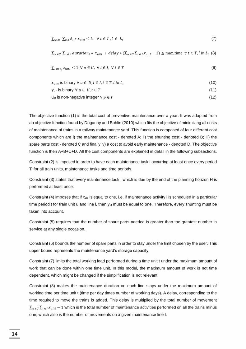
The objective function (1) is the total cost of preventive maintenance over a year. It was adapted from

an objective function found by Doganay and Bohlin (2010) which fits the objective of minimizing all costs

of maintenance of trains in a railway maintenance yard. This function is composed of four different cost

components which are i) the maintenance cost - denoted A; ii) the shunting cost - denoted B; iii) the

spare parts cost - denoted C and finally iv) a cost to avoid early maintenance - denoted D. The objective

function is then A+B+C+D. All the cost components are explained in detail in the following subsections.

Constraint (2) is imposed in order to have each maintenance task i occurring at least once every period

Ti for all train units, maintenance tasks and time periods.

Constraint (3) states that every maintenance task i which is due by the end of the planning horizon H is

performed at least once.

Constraint (4) imposes that if xuitl is equal to one, i.e. if maintenance activity i is scheduled in a particular

time period t for train unit u and line l, then yut must be equal to one. Therefore, every shunting must be

taken into account.

Constraint (5) requires that the number of spare parts needed is greater than the greatest number in

service at any single occasion.

Constraint (6) bounds the number of spare parts in order to stay under the limit chosen by the user. This

upper bound represents the maintenance yard’s storage capacity.

Constraint (7) limits the total working load performed during a time unit t under the maximum amount of

work that can be done within one time unit. In this model, the maximum amount of work is not time

dependent, which might be changed if the simplification is not relevant.

Constraint (8) makes the maintenance duration on each line stays under the maximum amount of

working time per time unit t (time per day times number of working days). A delay, corresponding to the

time required to move the trains is added. This delay is multiplied by the total number of movement

∑ ∑ 𝑥𝑢𝑖𝑡𝑙 − 1𝑖 ∈ 𝐼𝑢 ∈𝑈 which is the total number of maintenance activities performed on all the trains minus

one; which also is the number of movements on a given maintenance line l.

15

Constraint (9) imposes that, for each maintenance activity i of train u at a given time t is either not

performed (left hand side equal to zero) or performed in a given maintenance line (left hand side equal

to 1). The same maintenance activity i on the same train u can only be performed in one maintenance

line l.

Constraint (10) makes xuitl a binary variable for all train units, maintenance activities, time units and

maintenance lines.

Constraint (11) makes yut a binary variable for all trains and time units.

Constraint (12) imposes that Up is a non-negative integer for all spare parts.

3.7.1.1 Maintenance cost A

The maintenance cost A is the cost of doing every maintenance task over the planning horizon.

Each maintenance cost MA_costi must be given previously as an input; it corresponds to the cost of

doing a specific maintenance task i.

The cost component A can be expressed as the sum of all the maintenance costs of the maintenance

activities performed on every train, every line and at every time period until the horizon.

𝐴 = ∑ ∑ ∑ ∑ MA_cost𝑖

𝑙 ∈𝐿𝑖𝑡 ∈𝑇𝑖 ∈𝐼

∗ 𝑥𝑢𝑖𝑡𝑙

𝑢∈𝑈

3.7.1.2 Shunting cost B

The cost component B is the shunting cost; it corresponds to the cost of pulling a train out of its

regular duty in order to perform maintenance on this train. It can be expressed as the sum of the shunting

cost per time unit t of all trains stopped every time unit t of the planning horizon.

𝐵 = ∑ ∑ 𝑆 ∗ 𝑦𝑢𝑡

𝑡 ∈𝑇𝑢 ∈𝑈

3.7.1.3 Spare part cost C

The cost component C is the cost of keeping spare parts that need to be kept in good conditions

even when they are not used. The spare part cost is also defined previously by the user; it is commonly

estimated as a percentage of the initial price of the spare part. The cost component C can be set as the

product of the duration in time units of the planning horizon and the sum of the spare part cost times the

amount of each spare part. It must be highlighted that in this model, minimum amount of spare parts

16

remains the same throughout the year. Therefore, Up is chosen so that it would fulfil all maintenance

activities on all trains and all time periods over the planning horizon.

𝐶 = 𝐻 ∗ ∑ SP_cost𝑝 ∗ 𝑈𝑝

𝑝 ∈ 𝑃

3.7.1.4 Penalty cost D

The last cost component is a term to discourage early maintenance as it is both costly and likely

to trigger some early failure of the components. The cost component D can be seen as a penalty if the

last preventive maintenance before the end of planning horizon is performed too early. It is the product

of 1

(𝑢1−𝑢2)∗𝑁∗𝐻 which is a weighted penalty, times the distance between the last maintenance perfomed

and the end of the planning horizon (𝐻 − 𝑡) ∗ 𝑥𝑢𝑖𝑡𝑙 . The closer to the end of planning horizon the

maintenance activity is performed, the smaller the penalty cost is. The weighted penalty is made of the

inverse of the product of the total number of maintenance activities, multiplied by the planning horizon

times the number of spare trains; i.e. the difference between the number of train units owned by the

train operating company and the usefull number of trains to perform daily service.

𝐷 =1

(𝑢1 − 𝑢2) ∗ 𝑁 ∗ 𝐻 ∑ ∑ ∑ ∑(𝐻 − 𝑡) ∗ 𝑥

𝑢𝑖𝑡𝑙

𝑙 ∈𝐿𝑖𝑡 ∈𝑇𝑖 ∈𝐼𝑢∈𝑈

17

Model implementation and validation

In chapter 4, an illustrative example and its implementation is explained in detail in order to provide a

better understanding of the mathematical model. In a first subsection, the implementation in FICO

Xpress is described. In the second subsection, the parameters of the mathematical model are displayed

and in a third subsection the results of the mathematical model are explained.

4.1 Model implementation in FICO Xpress optimization software

Optimization has become a key parameter in nowadays industries as costs and system

complexity keep increasing over the years. Maintenance costs represent a major part in the total amount

of expenses for most transportation companies. This is why optimization solvers can have a major

impact on cost savings. An optimized maintenance is achieved either by maximizing or minimizing at

least one function, called objective function. In order to optimize the chosen objective function, an

important number of software with optimization solvers can be found online such as Excel; Gurobi; IBM

CPlex or FICO Xpress.

"As the premier mathematical modelling and optimization solution in the world, Xpress allows operations

researchers, analysts, consultants and others to easily create, deploy and utilize business optimization

solutions based on scalable high-performance algorithms, a flexible modelling environment and rapid

application [...].” (FICO 2015)

FICO Xpress is a software that enables the user to select different kind of solvers in order to create the

mathematical model that will correspond to the real case needing optimization. A non-exhaustive list of

solvers that can be chosen is quadratic solvers; nonlinear solvers, mixed-integer linear solvers. In

Fertagus case study, the objective function is linear and hence, the constraints are linear as well and

the decision variables are integers. This is why a mixed-integer linear solver was selected among the

ones available in the software.

Once the solver is selected, the mathematical model itself has to be created. Thus, it is interesting to

point out that it has a specific language, called Mosel, needed to write down the required objectives.

Indeed, for optimizing one parameter, it is required to write both an objective function and constraints.

The objective function is the expression that Xpress algorithm will either maximize or minimize. The

constraints, which restrict the model solution, are the limitations of the problem.

Depending on the parameters and constraints of the problem under analysis, the technical planning

would not be the same. Therefore, they have to be adapted for each specific case. The program is

divided in four steps which are: first initialization from data files, then the objective function expression,

the choice of the constraints of the system and finally the creation of a file with the output values.

18

The first step of the model (i.e. initialization) sets the parameters of the case study. In order to make

every input changes easier for the user; all parameters are controlled through an excel file which is then

converted into data files directly read by the program. This way of controlling inputs was chosen because

of the size of the problem; it was indeed confusing to declare all parameters directly in the mathematical

model.

In order to have an output more user-friendly than simply presenting the values of the decision variable

xuitl; the creation of a result file was added in the FICO Xpress program. In order to be able to do this,

two parameters are required: MA_typei and SP_typep. For every i, MA_typei is the name of the

maintenance activity i, while for every p SP_typep is the name of the spare part p. Once the optimization

calculus is over, the result file reads for each week of the planning horizon the value of the decision

variable xuitl for every train u, maintenance activity i and line l. If xuitl is equal to one, then a sentence is

written in the result file stating that “MA_typei has to be performed on line l on train u”. Otherwise if xuitl

equal to zero, nothing is written in the output file. Furthermore, the second output of the mathematical

model is the minimal amount of spare parts needed to perform the technical planning. In order to know

easily how many spare parts of each kind are needed, a sentence is written for every spare part type p

stating that “Minimal amount of SP_typep is Up”.

4.2 Parameters of an illustrative example

Model validation consisted in solving a small-scale example and analysing in details its

corresponding solution which is presented in this section. In this example, the studied company has 5

trains going to a maintenance yard in which three kinds of maintenances activities can be performed: i1,

i2 and i3. Two different spare parts are kept in order to be switched with parts mounted on trains: p1 and

p2.

The goal of the program is then to find the best technical planning possible, which means the technical

planning that will have the smallest cost over a planning horizon of 15 weeks.

Tables 3 to 7 provide values for the parameters used in this mathematical model created to represent

this example.

Table 3 : Constant used in the mathematical model of the illustrative example

Constants Units Values

H Weeks 15

S Monetary units 500

k Working hours 160

max_time Hours 40

N Without units 3

delay Without units 0.16

u1 Without units 6

u2 Without units 5

19

In Table 3, all the constants of the mathematical model are displayed. First the planning horizon which

is 15 weeks, then the shunting cost which is 500 monetary units. The maximum working load per week

is 160 working hours and the maximum working time is 40 hours. The maximum working load is

calculated by the product of the working time per day times the number of men working per day times

the number of useful days in a week. In the illustrative example that would be: k = 8 hours * 4 men * 5

(days) = 160 working hours. The maximum working time per week is simply the maximum working load

divided by the number of man working.

Table 4 : Information about maintenance activities

i MA_typei MA_costi Ti

(in weeks)

i

(in hours)

durationi

(in working

hours)

Li

1 i1 80 5 7 3,5 {1,2}

2 i2 100 30 20 5 {1,2,3}

3 i3 50 16 11 3,37 {1}

In Table 4, the first line for example is giving information about maintenance activity 1, first the name of

the maintenance activity 1 (i1), then its cost in monetary units (80). The next columns give the period of

maintenance activity 1 (5 weeks), the work load (7 working hours), the duration (3,5 hours) and finally

the set of maintenance lines where maintenance activity 1 can be performed ({1,2}). Maintenance

activity 1 can be done either on line 1 or one line 2 of the maintenance yard.

Table 5 : Information about spare parts

p SP_typep SP_costp

(per week)

Spare part

maintenance

duration (in weeks)

(Rp)

maximum amount

of spare part

(Ap)

1 p1 20 1 20

2 p2 30 2 20

In table 5, information about the spare parts can be found. For example, the first line gives information

about spare part 1, first the name of the spare part (p1), then cost of the spare part 1 per week (20

monetary units). The next columns give the maintenance duration of the spare part 1 (one week), and

the maximum amount of spare part 1 that be stored in the maintenance yard (20 units).

20

Table 6 : Distance in weeks between the last maintenance activity and beginning of planning horizon for each train

unit

In table 6, the initial conditions of all trains can be found. In the first line, for example, the initial conditions

of train 1 are stated, maintenance activity 1 (called i1) was performed 4 weeks before the beginning of

the planning horizon. Maintenance activity 2 (called i2) was performed 15 weeks before the beginning

of the planning horizon. Maintenance activity 3 (called i3) was performed 11 weeks before the beginning

of the planning horizon.

Table 7 : Number of spare part used for each maintenance activity

Maintenance

Activity

Spare part

i1 i2 i3

p1 1 0 1

p2 0 1 1

In table 7 displays which kind of spare part is used for which maintenance activity. In the first line the

following indications can be seen, one spare part 1 (called p1) is needed to perform maintenance activity

1 (called i1); no spare part 1 is needed to perform maintenance activity 2 (called i2). Finally, one spare

part 1 is needed to perform maintenance activity 3 (called i3).

4.3 Results of the optimization model

Once the algorithm converges to a solution, the program displays the minimum cost found for

the technical planning over 15 weeks, as well as the minimum number of spare parts required to fulfil

the technical planning (Figure 2). A data file with the technical planning inside is created, and enables

to build the planning shown in Table 8.

Maintenance Activity

Train number

i1 i2 i3

1 4 15 11

2 2 18 1

3 4 12 11

4 3 26 1

5 3 9 8

21

Table 8 : Technical planning of the illustrative example

Week number 1 2 3 4 5 6 7 8 9 10 11 12 13 14 15

Train 1

i1 X X X

i2 X

i3 X

Train 2

i1 X X X

i2 X

i3 X

Train 3

i1 X X X

i2

i3 X

Train 4

i1 X X X

i2 X

i3 X

Train 5

i1 X X X

i2

i3 X

From the technical planning, several facts can be highlighted. First, it can be seen that the period of the

maintenance activities is respected if nothing interferes. For train 3 for example, maintenance activity i1

is performed every 5 weeks as required by the user inputs (on Table 4 : Information about maintenance

activitiesTable 4). The period can be shorter when another maintenance task is scheduled few weeks

before the optimal date in order to share the shunting costs. It can be seen for train 2, when maintenance

i2 is performed on week 8, which is four weeks ahead of the deadline.

Interestingly, no maintenance 2 was performed for train 3 as the period of this maintenance is set to be

30 weeks, and it was performed 12 weeks before week 1. This implies that, during the next planning

horizon, train 3 will probably go to under maintenance 2 at most on week 3 (30-12-15 =2).

The first maintenance activity i1 of train unit 2 is performed on week 3 as it was done two weeks before

the beginning of the planning horizon; i1 is then performed on week 8, after five weeks – which is the

period of i1. Train 2 is under maintenance i2 on week 8; instead of week 12 if the period of 30 weeks was

strictly followed (30–18 =12). Indeed, i1 is to be performed on week 8 as well and shunting costs can be

shared if the two maintenance activities are performed together. Of course, doing i2 on week 13 with i1

could be tempting as it is closer to week 12, but i2 would then be performed one week late which is

impossible.

22

Figure 2 : Total cost and amount of spare parts of the illustrative example

In order to be able to fulfil the optimized technical planning; three spare parts p1 and two spare parts p2

are needed as pointed out in Figure 2. The number of spare part is not varying depending on time

because it is assumed that no spare parts are bought during the planning horizon.

The maintenance line number is also chosen within the possible set Li specified by a user input. In the

example, i1 can be performed on lines 1 and 2 which means that the model indicates that the

maintenance activity is to be done either on line 1 or line 2. In the Figure 3 below is giving the

assignments for the first week of the technical planning. In this file, information can be found about which

train is going under maintenance on a given line l of Li.

Figure 3 : First week of the example’s technical planning

As the size of the problem is relatively small, it can be seen that the time duration for the model

to get to a nil gap is a tenth of a second (Figure 4). It must be said that computational time will increase

if either the number of train units increases or the number of possible maintenance activities, spare parts

or lines is larger.

23

Figure 4 : Calculation duration

Figure 5 is an output from FICO Xpress software that delivers useful information such as the size of the

matrix before (Table 9) and after pre-solving stage, as well as information on the final solution (Table

10).

Table 9 : Explanation of the calculus of the column of the matrix

The matrix column’s size is calculated thanks to the size of each set of the mathematical model. All

decision variables have a size which is the product of the size of the sets of their corresponding indices.

For example, xuitl is made of the variables u, I, t and l, hence its size is the product of the size of variables.

In total, the matrix is made of 752 columns before pre-solving stage. This stage enables to supress

some of the redundancy within the initial matrix which reduces its size. The pre-solving process is

specific to FICO Xpress and is not accessible to the user.

Set Size

u={1,…,5} 5

i={1,…,3} 3

t={1,…,15} 15

l={1,…,3} 3

p={1,2} 2

decision variables

size

xuitl 5*3*15*3=675

yut 5*15=75

Up 2=2

Size of the columns

675+75+2=752

24

Table 10 : Solution information

Solution information Value

Best bound 11050,8 monetary units

Best solution 11050,8 monetary units

Gap 0 %

Computational time 0,1 seconds

In Table 10, all the useful information about the solution that was found are given. The best bound of

the objective function is in this case the best lower bound, as this objective is to find a minimum. In the

illustrative example, it is interesting to underline that the solution is optimal because the optimality gap

is zero. The optimality gap is indeed the ratio, converted in percentage, of the difference between the

solution of the total cost and the best bound of the cost.

𝑜𝑝𝑡𝑖𝑚𝑎𝑙𝑖𝑡𝑦 𝑔𝑎𝑝 = 𝑡𝑜𝑡𝑎𝑙 𝑐𝑜𝑠𝑡 𝑠𝑜𝑙𝑢𝑡𝑖𝑜𝑛 − 𝑙𝑜𝑤𝑒𝑟 𝑏𝑜𝑢𝑛𝑑

𝑡𝑜𝑡𝑎𝑙 𝑐𝑜𝑠𝑡 𝑠𝑜𝑙𝑢𝑡𝑖𝑜𝑛∗ 100

In this illustrative example, the computational time to achieve a nil gap was a tenth of a second because

the size of the problem was small. However, in larger size problems the computational time increases

and the optimality gap is a good indicator of the optimality of the solution when the computation is

stopped. The smaller the optimality gap, the closer the solution is to the optimal value.

25

The Case study of Fertagus train operating company

In chapter 5, Fertagus train operating company is presented briefly and problem specifications are

introduced. The parameters of mathematical model are displayed in a table with all cost values given in

monetary units for the sake of confidentiality.

5.1 Fertagus train operating company

As depicted in Figure 5, Fertagus trains run on a line of 54 kilometres that crosses the “25 de

Abril” bridge and stop at 14 stations. Total travel duration between Roma-Areeiro and Setúbal is 57

minutes and the bridge crossing is only 7 minutes long.

Figure 5 : Fertagus' railway map (source: Fertagus website)

Fertagus is a train operating company whose name derives both from "caminhos-de-ferro" and the

Tagus river's name. It became the first private rail operator in Portugal when it won the call for bids for

the line between Lisbon's city centre and the Setubal district area. As a result, it now has a contract that

ensures availability, cost and duration of travels. As it was the first private railway operator in Lisbon

metropolitan area, it is interesting to realize that availability is part of the contract with Lisbon’s city

centre. Indeed, in order to optimize maintenance, it must be kept in mind that no train can be pulled out

of service to go to maintenance if there is no backup train available. In order to guarantee that this would

26

not happen, Fertagus chose to have eighteen trains when only seventeen are necessary to perform the

current operation schedules. The question of whether or not this could be done differently is out of the

scope of the present work and is left for further research. However, it might not be necessary to have

an additional train if instead of doing mileage-based maintenance, Fertagus was using a condition-based

maintenance approach.

It must be said that as Fertagus does not own the railway line, infrastructure charges must be paid to

the infrastructure manager, IP, and the railway infrastructure maintenance is not up to Fertagus. This

also means that Fertagus trains are not the only trains running over the line between Roma-Areeiro and

Setubal, which might result in technical issues as not all trains have the same requirements. Indeed,

during one of the visits to the maintenance yard, Eng. João Duarte told us that since the line started to

be used by other trains going faster, unusual wear was noticed on all the trains’ wheelsets. Nevertheless,

this might also be due to the wheelsets that have replaced the old ones. A more detailed analysis is

needed and is also left to further research.

During this work, three meetings with Fertagus staff were scheduled and some additional information

was given by email and phone calls. This work benefited from two main contacts, Engineer João

Grossinho and Engineer João Duarte in the maintenance yard of Fertagus.

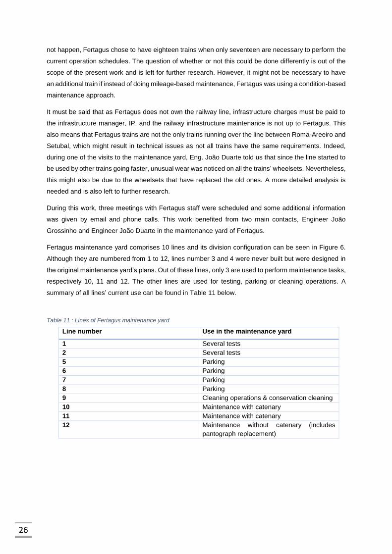
Fertagus maintenance yard comprises 10 lines and its division configuration can be seen in Figure 6.

Although they are numbered from 1 to 12, lines number 3 and 4 were never built but were designed in

the original maintenance yard’s plans. Out of these lines, only 3 are used to perform maintenance tasks,

respectively 10, 11 and 12. The other lines are used for testing, parking or cleaning operations. A

summary of all lines’ current use can be found in Table 11 below.

Table 11 : Lines of Fertagus maintenance yard

Line number Use in the maintenance yard

1 Several tests

2 Several tests

5 Parking

6 Parking

7 Parking

8 Parking

9 Cleaning operations & conservation cleaning

10 Maintenance with catenary

11 Maintenance with catenary

12 Maintenance without catenary (includes

pantograph replacement)

27

Figure 6 : Plane view of Fertagus maintenance yard

In Figure 6, a plane view of Fertagus maintenance yard is shown. It can be seen that all lines used to

perform maintenance activities (lines 10, 11 and 12) are covered by a roof in order to avoid rain falling

on trains while they are being maintained. On the contrary, line number 9 which is dedicated to cleaning

is not covered because this maintenance activity is to be performed outside; this line is located on the

left of the maintenance yard. Fertagus maintenance yard also performs wheelset turning within the

maintenance yard in an underfloor room that is shown on the figure above.

5.2 Specific input parameters for MILP formulation

In order to model the present case study, some information about the maintenance activities

was gathered in order to have the correct inputs for the parameters of the mathematical model. During

meetings, Fertagus maintenance activities were explained by Eng. João Grossinho and Eng. João

Duarte and summarized on the tables below. While the first one corresponds to the maintenance

activities scheduled by Fertagus maintenance crew; the second table sums up the maintenance

activities scheduled by a consultancy company which provides support for major renewals. Because of

the way the program was built, only the maintenance activities scheduled by Fertagus maintenance

crew could be taken into account. The integration of R1, R2 and R3 major renewals in the mathematical

model is left for further research.

Table 12 : Maintenance tasks which are not performed by Fertagus crew

Maintenance

activity

Tasks performed

during MA Period

Time

needed to

perform MA

Men force

required Cost

R3 Pantograph are replaced Every 600,000 km

Unknown Unknown Unknown

R2

replacement of wheelsets, bogies are repaired and sent to EMEF or RENFE

Every 1,200,000 km

Unknown Unknown Unknown

R1

replacement of wheelsets, bogies are repaired and sent to EMEF or RENFE

Every 1,800,000 km

Unknown Unknown Unknown

28

Table 13 : Maintenance tasks performed by Fertagus crew

Maintenance

activity

Tasks performed

during MA

Period Time needed

to perform MA

Men force

required

ETS "Ensaios e Trabalhos Sistemáticos”

Mostly inspection activities

Every 5 weeks 1h30-2h00 4

VEq “Visita de Equipamento”

Inspection of motor block, pressure check, etc.

Every 37,500 km 6h00 4

VP “Visita de Portas”

Doors check-up Every 150,000 km 6h00 4

VL “Visita de Lubrificação”

Lubrication check-up

Every 120,000 km 4h00-6h00 4

VEl “Visita Eléctrica”

Electric system check-up

Once a year (before winter)

40h00 (not continuous)

4

VS “Visitas Sazonais”

Biannual check-up Twice a year (beginning of Spring and end of Summer)

12h00 4

TRF “Torneamento dos rodados”

Wheelsets turning Every 120,000 km 16h00 during weekend

2

V1 Some parts of the pantograph are maintained

Every 300,000 km Unknown 4

The mathematical model’s parameters for the Fertagus case study were extracted from the two tables

above and completed through additional meetings; emails or phone calls. All parameters used for the

Fertagus case study can be found in the following tables (Table 14, Table 15, Table 16, Table 17, Table

18 and Table 19).

Table 14 : Sets of the mathematical model

Sets Values

U {1,...,18}

I {1,...,16}

T {1,…,53}

P {1,…,4}

In Table 14 the sets of Fertagus case study are displayed; they are eighteen trains so U is a set of

integers going from 1 to 18. Furthermore, sixteen maintenance activities can be performed in Fertagus

maintenance yard which implies that i is a set of integers from 1 to 16. The planning horizon of the

technical planning is a year so, since the time unit is a week, T is a set of integers from 1 to 53. It is true

that a year is made of less than 53 weeks, but as it is also more than 52 weeks; the horizon was chosen

to stop at week 53 in order to include the few days remaining after week 52. Finally, 4 different spare

parts are stored in Fertagus maintenance yard so P is a set of integers from 1 to 4.

29

Table 15 : Parameters of the mathematical model depending on the maintenance activity i

i MA_typei MA_costi Ti (in weeks) i (in working hour)

durationi Li

1 ETS 614,42 5 10 2,5 {10 11}

2 VEQ 1720,37 16 28 7 {10 11}

3 LUB 1018,98 53 14 3,5 {10 11}

4 POR 829,17 63 14 3,5 {10 11}

5 TRF 2522,22 63 42 21 {10 11}

6 LL 815,28 63 14 4,6 {10 11}

7 ELET1 3516,44 53 12,4 3,1 {10 11}

8 ELET2 3516,44 53 12,4 3,1 {10 11}

9 ELET3 3516,44 53 12,4 3,1 {10 11}

10 ELET4 3516,44 53 12,4 3,1 {10 11}

11 ELET5 3516,44 53 12,4 3,1 {10 11}

12 AC 793,29 53 14 7 {10 11}

13 BAT1 396,64 53 3,5 0,88 {12}

14 BAT2 396,64 53 3,5 0,88 {12}

15 MR 56,25 26 1 1 {10 11}

16 V1 2457,68 136 40 10 {12}

In Table 15 all parameters depending on the maintenance activities i are summarized. The first line

includes the name of maintenance activity 1 which is ETS, its cost in monetary units which is 614,42.

Then the period of the ETS maintenance is displayed in weeks and is equal to five weeks. This means

that maintenance activity 1 (called ETS) is due every five weeks. Then, both the working load and the

duration of the maintenance activity 1 are given. ETS maintenance is a 10 working hours maintenance

activity and lasts 2,5 hours long. Because the working load and the duration are linked by the relation

“working load = duration * working men”, it can be deduced that currently 4 men are needed to do

maintenance activity 1. Finally, the set of maintenance lines where maintenance activity 1 can be

performed is displayed. It can be read that maintenance ETS can be performed either on line 10 or on

line 11 of Fertagus maintenance yard. Indeed, it was explained in Table 11 that line 10 and 11 are

equipped with the same tools and can therefore be used for the same maintenance activities.

Table 16 : Parameters of the mathematical model depending on the spare parts p

p SP_typep SP_costp Rp Ap

1 wheelset 104,17 1 20

2 trailer bogie 1041,67 0 20

3 motor bogie 1041,67 1 20

4 pantograph 416,67 2 20

Parameters that depends on the spare parts p are displayed in Table 16. In the first line, all information

about the spare part 1 is given; the first piece of information is the spare part’s name which is a wheelset.

Then, the cost of the spare part 1 per week is given in monetary units and is 104,17. The next parameter

30

is the number of weeks needed to maintain the spare wheelset and its value is one which means that

when a spare wheelset is sent to maintenance it will be unavailable for one week. Finally, the maximum

number of spare parts 1 is given according to the maintenance yard storage area. Because Fertagus

maintenance yard is relatively large, it is assumed that storage would not be an issue; this is why the

maximum number of wheelsets is set to 20. Here the largest number of spare parts does not constraint

the solution, it only reduces the number of values that the solver will test. Thus, it reduces the

computational time.

Table 17 : Time interval between last maintenance activity i and beginning of planning horizon for train u

Train number\MA 1 2 3 4 5 6 7 8 9 10 11 12 13 14 15 16

1 4 3 19 50 46 25 40 40 40 40 40 13 16 16 19 45

2 2 5 26 7 42 25 40 40 40 40 40 13 16 16 9 40

3 4 0 37 19 20 24 36 36 36 36 36 12 16 16 16 54

4 3 10 40 30 15 20 35 35 35 35 35 12 16 16 18 56

5 3 15 16 16 15 24 15 15 15 15 15 12 15 15 24 56

6 0 14 2 42 36 23 14 14 14 14 14 11 15 15 3 54

7 3 15 18 23 49 23 13 13 13 13 13 11 15 15 17 47

8 0 1 30 30 51 22 12 12 12 12 12 10 14 14 4 55

9 1 14 38 14 47 22 12 12 12 12 12 10 14 14 11 46

10 1 0 5 37 39 21 11 11 11 11 11 9 14 14 0 35

11 3 9 43 16 44 21 10 10 10 10 10 9 13 13 5 41

12 4 11 52 45 43 20 7 7 7 7 7 8 13 13 6 35

13 2 10 17 3 45 20 6 6 6 6 6 8 13 13 18 41

14 2 14 13 48 46 19 5 5 5 5 5 7 12 12 16 35

15 4 6 33 22 40 19 4 4 4 4 4 7 12 12 8 49

16 0 1 46 45 36 18 3 3 3 3 3 6 12 12 23 37

17 3 15 39 55 48 18 2 2 2 2 2 6 11 11 20 43

18 4 12 28 35 35 17 1 1 1 1 1 5 11 11 14 44

Initial conditions about Fertagus trains can be found in Table 17. The different maintenance activities

are put in the columns while the different lines correspond to different trains. The first line set all the

initial conditions for train 1. The first value is the distance between the last maintenance activity 1 and

the beginning of the planning horizon and is 4; which means that the last maintenance activity 1 (called

ETS) was performed on train 1 four weeks ago. It must be highlighted that all values of Oui can be

deduced from this table. For example, O23, which corresponds to the last time maintenance activity 3

was performed on train 2, is set to 23 weeks in the above table. Therefore, maintenance activity 3 was

done 23 weeks before the beginning of the planning horizon.

31

Table 18 : ip parameter of the mathematical model

SP\MA 1 2 3 4 5 6 7 8 9 10 11 12 13 14 15 16

1 0 0 0 0 1 0 0 0 0 0 0 0 0 0 0 0

2 0 0 0 0 0 0 0 0 0 0 0 0 0 0 0 1

3 0 0 0 0 0 0 0 0 0 0 0 0 0 0 0 1

4 0 0 0 0 0 0 0 0 0 0 0 0 0 0 0 1

Table 18 summarizes the values of parameter ip which is the amount of spare part p required to perform

maintenance activity i. Sixteen different maintenance activities can be done in Fertagus maintenance

yard; but they do not all require the same spare parts. Most of Fertagus maintenance activities, such as

maintenance activity 1, do not need any spare part. This can be seen on the first column of the above

table, where all values are set to zero. It must be said that spare parts are mostly used during corrective

maintenance in Fertagus case study which is why the cost of preventive maintenance is lower. However,

some maintenance activities of Fertagus railway operating company still need spare part to be done. It

is the case of maintenance activity 5 that requires one spare part one (which is a wheelset) to be

performed.

Table 19 : Constants of the mathematical model

Constants Units Values

H weeks 53

S monetary units 5000

k working hours 160

max_time hours 40

N without units 17

delay hours 0.16

u1 without units 18

u2 without units 17

All constants of the mathematical model can be found in Table 19. First the planning horizon H whose

value is 53 weeks. It is true that a year is made of less than 53 weeks, but as it is also more than 52

weeks; the horizon was chosen to stop at week 53 in order to include the few days remaining after week

52 The shunting cost is then set to 5000 monetary units, this value was initially given as an

approximation and will thus be the subject to a sensitivity analysis in the next chapter. The maximal

working load k which is 160 working hours is calculated as the product of the number of men working in

Fertagus maintenance yard by the number of working hours per day times the number of useful days of

the week. In the case study it is then, 4 men * 8 hours * 5 (days) = 160 working hours. The maximal

working time per week is 40 hours and is calculated as the product of the number of working hours per

day times the number of useful days in a week. In Fertagus case study it is 8 hours * 5 (days) = 40

hours. It is interesting to notice that the maximal working load and the maximal working time are related

to one another with the equation working load = working time * number of men.

32

33

Results and Discussion

In chapter 6 several studies can be found. Firstly, an analysis of the optimality gap over calculation time.

In the next subsections, a sensitivity analysis of both the shunting cost component and the maximal

working time per week.

6.1 Results of Fertagus case study

This section displays the result of the optimization of Fertagus case study after one hour computation.

It must be said that the mathematical model had been stopped before it could reach an optimal solution.

In the next subsections, the influence of several parameters will be studied, but the reference case is

the following one. The output data about the matrix from the software can be found in Figure 7.

Figure 7: Computation data of Fertagus case study

In Figure 7 above, the same output of computational data as in the illustrative example can be find.

However, the case study has a much larger size than the illustrative example. Indeed, the matrix has

46750 columns, which is sixty times more than the illustrative example. With a larger matrix, the

computational time to get an optimal value is expected to increase; indeed, after one hour the solution

34

for the total cost of preventive maintenance is still not optimal but has an optimality gap of 0,63%. An

analysis of the optimality gap as a function of calculation time is done in the next subsection.

The best solution is a preventive maintenance cost of 1664750 monetary units; this cost is divided into

four cost components A, B, C and D whose values are displayed in Table 20.

Cost component Value (monetary units) Percentage of the total cost

A (maintenance activity cost) 670495 39,89%

B (shunting cost) 1005000 59,78%

C (spare part cost) 5521,01 0,33%

D (penalty cost) 15,5 0,0009%

Table 20: Values of the cost components

In Table 20, the cost components percentage can be seen. The cost component B is the one with the

largest impact on the total preventive cost which is why maintenance activities are grouped whenever it

is possible. The cost component A, which is the maintenance activity cost, has the second largest

impact. However, it is not a cost that is easily changed as it is dependent on the maintenance activities

themselves. The cost components C and D have smaller influence on the total preventive maintenance

cost.

6.2 Analysis of the optimality gap as a function of calculation time

As it was said in chapter 3, when the size of the problem increases, so does the computational

time to get to the optimal solution. Indeed, if optimality of the solution is not taken in consideration, then

a feasible solution can always be found within few minutes. However, if optimality of the solution is

important, the gap corresponding to the feasible solution is an indicator of the optimality of the solution.

The closer the gap is to zero, the better the solution is. When the size of the problem is relatively small

(such as the illustrative example that has 752 variables), the optimal solution can be found in a tenth of

a second as it was the case in the illustrative example. Nevertheless, in the case of Fertagus the

computational time is much larger, due to a significant increase of the size of the sets. It is then

interesting to study the evolution of the gap with respect to computational time in order to know when

the solution can be considered as satisfying. Indeed, most of the time the calculus is stopped before the

exact solution is reached (i.e. when the gap is 0) in order to save computational time.

In this analysis, the computational time was increased from 1 minute to 24 hours, and the graph of gap

versus computational time can be found in Figure 8. The goal of this study is to be able to select the

smallest computational time, whose corresponding optimality gap is acceptable. It can be seen on the

graph that after a calculation time of one hour, an optimality gap of around 0,6% is achieved. When

computational time is increased to one day, the gap becomes slightly less than 0,5% which is better but

may not be worth the additional time spent to minimize the cost. Consequently, the computational time

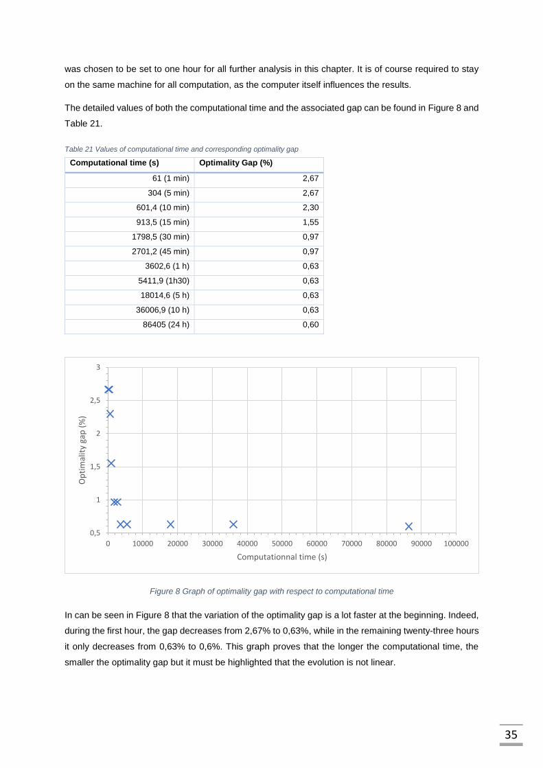
35

was chosen to be set to one hour for all further analysis in this chapter. It is of course required to stay

on the same machine for all computation, as the computer itself influences the results.

The detailed values of both the computational time and the associated gap can be found in Figure 8 and

Table 21.

Table 21 Values of computational time and corresponding optimality gap

Computational time (s) Optimality Gap (%)

61 (1 min) 2,67

304 (5 min) 2,67

601,4 (10 min) 2,30

913,5 (15 min) 1,55

1798,5 (30 min) 0,97

2701,2 (45 min) 0,97

3602,6 (1 h) 0,63

5411,9 (1h30) 0,63

18014,6 (5 h) 0,63

36006,9 (10 h) 0,63

86405 (24 h) 0,60

Figure 8 Graph of optimality gap with respect to computational time

In can be seen in Figure 8 that the variation of the optimality gap is a lot faster at the beginning. Indeed,

during the first hour, the gap decreases from 2,67% to 0,63%, while in the remaining twenty-three hours

it only decreases from 0,63% to 0,6%. This graph proves that the longer the computational time, the

smaller the optimality gap but it must be highlighted that the evolution is not linear.

0,5

1

1,5

2

2,5

3

0 10000 20000 30000 40000 50000 60000 70000 80000 90000 100000

Op

tim

alit

y ga

p (

%)

Computationnal time (s)

36

6.3 Analysis of maintenance costs as a function of shunting cost component

In Fertagus case, the shunting cost component value is set to 5000 monetary units. However,

this cost was provided as an approximated value so it was worth doing a sensitivity analysis on this

parameter of the mathematical model. In order to study the influence of the parameter on the total cost

of the maintenance, the shunting cost component is varied from 4500 monetary units to 5500 monetary

units. This corresponds to an increase and a decrease by 10% of this cost component.

The graph of the total maintenance cost with respect to the shunting cost component can be found in

Figure 9. Another graph can be found in Figure 10 representing the variations in percentage of the total

maintenance cost induced by the variations in percentage of shunting cost component.

Figure 9 : Total maintenance cost versus shunting cost component

It can be seen in Figure 9 that the evolution of the total preventive maintenance cost is similar to a linear

evolution between 4500 and 5500 monetary units. The linear curve displayed on the above figure has

an equation that is y =18985x + 728178; this linear function values has a difference with the real value

of 0,2% in average.

y = 189,85x + 728178

1550000

1600000

1650000

1700000

1750000

1800000

4400 4600 4800 5000 5200 5400 5600

Tota

l mai

nte

nn

ance

co

st (

mo

net

ary

un

its)

Shunting cost S (monetary units)

37

Table 22 : Relation between the two variations

Shunting variation (%) Total maintenance variation (%) Relation between the two

variations

-10 -5,43 0,54

-8 -4,12 0,51

-6 -3,54 0,59

-4 -2,63 0,66

-2 -0,90 0,45

0 0,00 Not relevant

2 1,30 0,65

4 2,97 0,74

6 3,58 0,60

8 4,46 0,56

10 5,68 0,57

Figure 10 : Variation of total cost with respect to shunting cost component variations

Two different curves can be found in Figure 10, one is called “regular values and the other is “absolute

values”. The first one, with “regular values”, corresponds to the variation in percentage of the total

maintenance cost with respect to the variation in percentage of shunting cost (between the reference

value 5000 and the value used in the mathematical model). The other curve the “absolute values”

corresponds to the absolute value of the variation in percentage of the total maintenance cost, with

respect to the variation in percentage of shunting cost.

A variation of the shunting cost of 2% induces a variation of total maintenance variation of 1,3% which

corresponds to a relation of 0,65 between the total maintenance variation and the shunting cost

-7

-5

-3

-1

1

3

5

7

-11 -9 -7 -5 -3 -1 1 3 5 7 9 11

shunting

Variation of shunting cost (%)

absolute values

regular values

38

variation. In Table 22 a summary of the relations between shunting cost component and total

maintenance variations. The average value of these relations is 0,58 which means that the variation of

shunting cost component induces a smaller variation of the total maintenance cost.

It is interesting to notice that the “absolute values” curve in Figure 10 : Variation of total cost with respect

to shunting cost component variationsFigure 10 is nearly symmetric with respect to the y-axis. It means

that an increase of 3% of the shunting cost component will induce a raise on the total cost; and this raise

has the similar absolute value than the diminution of the total costs induced by a decrease of 3% in the

shunting cost component. It must be said that the values induced by a negative shunting variation are

always slightly higher than the ones induced by a positive shunting variation. For instance, a variation

of the shunting cost of -2% induces a total cost variation of 0,90% while a variation of shunting cost of

+2% induces a total cost variation of 1,30%

The relation between the shunting variation in percentage and the total maintenance variation in

percentage can be found in Table 22. The value for a variation of zero percent is not considered to be

relevant as a division by zero would be involved otherwise. It is interesting to highlight that all the ratio

between the total maintenance variation and the shunting variation are always smaller than one which

means that the variation of total cost is damped with respect to the shunting cost variation.

6.4 Analysis of total maintenance costs as a function of working time per week

Fertagus preventive maintenance is done in a shift of 8 hours per day, and five days a week;

which corresponds to a current maximum working time in the maintenance yard of 160 hours/week. In

order to quantify the impact of the time allocated to preventive maintenance, an analysis was performed

in order to assess the evolution of total maintenance costs with respect to the evolution of the maximum

working time. It must be highlighted that even if only the maximum working time value changes, it affects

two parameters of the mathematical model which are k and max_time (the maximum working load per

week and the maximum working time per week).

The graphs in Figure 11 and Figure 12 show the variation of the total maintenance costs and the

optimality gap as a function of the variation of the time allocated to preventive maintenance per week.

The time allocated varies from 144 working hours to 176 working hours; 160 working hours being the

reference (all values can be found in Table 22). When the time allocated is 144 working hours, there is

no value for the gap nor for the total maintenance costs because no feasible solution could be found.

On the contrary when the time allocated is 176 working hours, the optimal solution is find in 2445,8

seconds (40min and 45 seconds) which means the calculus stops before the end of the reference

computational time. For an allocated time of 168 working hours the solution is optimal after 2684

seconds (44 min and 46 seconds).

39

Table 23 : Values of gap and total maintenance costs for different time duration

allocated working hours per

week

allocated hours per

week

gap after one hour

(%)

total maintenance cost

(monetary units)

36 144 - No feasible solution

38 152 1,84 1701030

40 160 0,63 1675360

42 168 0 1659800

44 176 0 1659750

Figure 11 : Graph of optimality gap versus time allocated per week

Figure 12 : Graph of total maintenance costs versus time allocated per week

The horizontal axis of Figure 11 and Figure 12 are the same, which is logical considering that the working

load allocated and the working time allocated are related through the equation:

load = working time * number of men. During the sensitivity analysis, the number of men does not

change which explains why only one parameter was used to plot the graph of the sensitivity analysis.

0

0,2

0,4

0,6

0,8

1

1,2

1,4

1,6

1,8

2

150 155 160 165 170 175 180

Op

tim

alit

y ga

p (

%)

working load allocated to preventive maintenance (man-hours)

1655000

1660000

1665000

1670000

1675000

1680000

1685000

1690000

1695000

1700000

1705000

150 155 160 165 170 175 180

Tota

al m

ain

ten

ance

co

st (

mo

net

ary

un

its)

work load allocated to preventive maintenance (working hours)

40

On Figure 11 it can be noticed that the optimality gap value is increased three times when the working

load is lower than 160 working hours. If the working load is lower than 152 working hours, something

curious appears, there is no feasible solution that can be found. There are two possible explanations for

this; either 160 working hours working load for preventive maintenance is considered optimal in Fertagus

case study; or the initial conditions have a lot of influence on the technical planning. Indeed, a

maintenance which is done by four working men for several planning horizons could lead to initial

conditions that require a preventive maintenance done by four men. Therefore, after having performed

preventive maintenance a certain way for a long time it could be difficult to change the way to do things.

On Figure 12, the total cost of preventive maintenance is decreasing when the working load increases.

Indeed, maintenance activities that have to be performed on a given week are the same no matter the

allocated working load. However, it is easier to schedule maintenance activities if the working load is

not restrictive. This is why the total cost of preventive maintenance is lower for a working load of 176

working hours than for a working load of 168 working hours; even if the solution is optimal in both cases.

On the contrary, if the working load is too low it may be impossible to schedule maintenance activities,

it is the case when the working load is 144 working hours.

41

Conclusions and Future Research

In the final chapter, the conclusion of the performed research can be found as well as some limitations

and possible further steps of the future research.

7.1 Conclusions

Optimizing the total costs of preventive maintenance is of course the objective of every

company, since it would have a non-neglectable effect on the budget. The goal of this dissertation was

to create a mathematical model that would provide an optimal technical planning, reducing the total

preventive maintenance costs to a minimum. The mathematical model created was adapted to the

specific case of Fertagus railway operator but can be very easily be modified to fit to any company’s

specifications. This adaptation involved collecting data related to maintenance activity operations in the

maintenance yard and some sensitive costs which are displayed in monetary units for the sake of

confidentiality.

One of the objectives of this dissertation was to prove that this program would give the optimal

feasible technical planning if at least one can be found. It is important to underline that whenever a

parameter was too restrictive, the mathematical model would say that no feasible solution could be

found. Several simulations were made in order to quantify the sensitivity of some parameters and the

mathematical model was considered satisfying.

Moreover, it is interesting to realize that the mathematical model is able to give a feasible

solution with an optimality gap of less than one percent in less than one hour. Indeed, most company

would care about the optimality of the solution. This is why, even if a technical planning is performed

once a year, it is still compelling that the computational time for a Fertagus size stays relatively low.

7.2 Limitations

This mathematical model enables to find an optimal technical planning but it is of course user

input dependent and this is a major limitation. Indeed, if the user inputs do not represent correctly the

real-life situation, the technical planning could hardly be optimal, even if an optimal solution is found.

This is the case in Fertagus maintenance yard, which means that the solution found is actually not the

best possible. Indeed, some maintenance activities are performed by Fertagus maintenance crew, but

some others (such as R1, R2 and R3) are scheduled by a consultant company. These maintenance

activities were not taken into consideration and consequently the total maintenance cost found by the

program might not be the actual optimal one.

42

7.3 Future Research

As mentioned in the previous subsection, all maintenance activities scheduled by a consultancy

company are not taken into account. In order to provide a total maintenance costs which would be more

accurate, a new cost component will have to be added. This cost component should reflect the cost of

having these maintenance activities done outside of Fertagus maintenance yard. It should be made of

both a cost of unavailability and a labor cost and will have to be added to the mathematical model.

Moreover, even if this dissertation provides a first approach of an optimized technical planning,

it must be kept in mind that the cost of preventive maintenance represents barely a half of the costs of

corrective maintenance. This means that if a company really wants to save costs on maintenance,

corrective maintenance should really be taken into consideration. In Fertagus case, corrective

maintenance is done every day during eight hours a day, right after the eight hours dedicated to

preventive maintenance. One way of taking into account corrective maintenance would be to add a

corrective maintenance cost component in the mathematical model. However, ideally a new program

should be created since corrective maintenance can only be predicted through predictive model while

preventive maintenance has fixed period.

Finally, it must be said that obtaining an optimal technical planning is only the first step. After

this, it must be verified that the optimal technical planning is feasible thanks to an operational planning.

Indeed, some of the constraints of the maintenance yard cannot be implemented in the technical

planning mathematical model. This highlights the fact that a new mathematical model, that would take

the optimal technical planning as an input, should be created. Indeed, with both an optimal technical

planning and an optimal operational planning found, the total maintenance costs of a company would

be significantly improved.

43

References

ALMGREN Torgny, ANDRÉASSON Niklas, PATRIKSSON Michael, et al. The replacement

problem: A polyhedral and complexity analysis. Technical report preprint 2009: 4. Göteborg:

Chalmers University, 2009.

BAZARGAN Massoud. An optimization approach to aircraft dispatching strategy with

maintenance cost–A case study. Journal of Air Transport Management, 2015, vol. 42, p. 10-

14.

BOHLIN Markus and WÄRJA Mathias. Maintenance optimization with duration-dependent

costs. Annals of Operations Research, 2015, vol. 224, no 1, p. 1-23.

DO Phuc, VU Hai Canh, BARROS Anne, et al. Maintenance grouping for multi-component

systems with availability constraints and limited maintenance teams. Reliability Engineering &

System Safety, 2015, vol. 142, p. 56-67.

DOGANAY Kivanc and BOHLIN Markus. Maintenance plan optimization for a train fleet. WIT

Transactions on The Built Environment, 2010, vol. 114, no 12, p. 349-358.

HAGHANI Ali and SHAFAHI Yousef. Bus maintenance systems and maintenance scheduling:

model formulations and solutions. Transportation research part A: Policy and Practice, 2002,

vol. 36, no 5, p. 453-482.

LAI Yung-Cheng Rex, WANG Shao-Wei, and HUANG Kwei-Long. Optimized Train-Set

Rostering Plan for Taiwan High-Speed Rail. IEEE Transactions on Automation Science and

Engineering, 2017, vol. 14, no 1, p. 286-298.

MARÓTI Gábor and KROON Leo. Maintenance routing for train units: The interchange model.

Computers & Operations Research, 2007, vol. 34, no 4, p. 1121-1140.

VU Hai Canh, DO Phuc, BARROS Anne, et al. Maintenance grouping strategy for multi-

component systems with dynamic contexts. Reliability Engineering & System Safety, 2014,

vol. 132, p. 233-249.

FICO® Xpress Optimization Suite, Educational license, http://www.fico.com/en/products/fico-

xpress-optimization-suite

CP Urban Services – Wikipedia, digital image, viewed 15 March 2017,

https://en.wikipedia.org/wiki/CP_Urban_Services

44

Diagrama de Rede Fertagus | Fertagus, digital image, viewed 15 March 2017,

https://www.fertagus.pt/pt/diagrama-de-rede-fertagus

European Commission, 2011, White paper on transport,

https://ec.europa.eu/transport/themes/strategies/2011_white_paper_en