Optimization of Electricity Retailer’s Contract Portfolio

University of Calgary

PRISM: University of Calgary's Digital Repository

Haskayne School of Business Haskayne School of Business Research & Publications

2010

Optimization of Electricity Retailer’s Contract

Portfolio Subject to Risk Preferences

Kettunen, Janne; Salo, Ahti; Bunn, Derek W

Institute of Electrical and Electronics Engineers (IEEE)

J. Kettunen, A. Salo, and D.W. Bunn. Optimization of Electricity Retailer’s Contract Portfolio

Subject to Risk Preferences. IEEE Transactions on Power Systems, 25(1):117–128, 2010.

http://hdl.handle.net/1880/47850

journal article

Downloaded from PRISM: https://prism.ucalgary.ca

IEEE TRANSACTIONS ON POWER SYSTEMS, VOL. 25, NO. 1, FEBRUARY 2010 117

Optimization of Electricity Retailer’s ContractPortfolio Subject to Risk Preferences

Janne Kettunen, Member, IEEE, Ahti Salo, and Derek W. Bunn

Abstract—When an electricity retailer faces volume risk inmeeting load and spot price risk in purchasing from the wholesalemarket, conventional risk management optimization methods canbe quite inefficient. For the management of an electricity contractportfolio in this context, we develop a multistage stochastic opti-mization approach which accounts for the uncertainties of bothelectricity prices and loads, and which permits the specification ofconditional-value-at-risk requirements to optimize hedging acrossintermediate stages in the planning horizons. Our experimentalresults, based on real data from Nordpool, suggest that the mod-eling of price and load correlations is particularly important. Thesensitivity analysis is extended to characterize the behavior ofretailers with different risk attitudes. Thus, we observe that a riskneutral retailer is more susceptible to price-related than load-re-lated uncertainties in terms of the expected cost of satisfying theload, and that a risk averse retailer is especially sensitive to thedrivers of the forward risk premium.

Index Terms—Electricity market, retailer’s contract portfoliooptimization, risk management, stochastic optimization.

I. INTRODUCTION

E LECTRICITY retailers face the problem of meeting in-stantaneous and variable loads which they may need to

satisfy by purchasing electricity from wholesale power marketsthrough spot and forward contracts. Optimizing this process issocially important and analytically challenging, incorporatingvolume as well as extreme price risks [1], [2]. Wholesale poweris increasingly being produced and traded via exchanges as anenergy commodity, but its stochastic characteristics and risks areinfluenced by its delivery as an essential service to end-users.As a consequence, with companies facing uncertainties abouttheir future loads as well as prices, the development of opti-mization models that allow power utilities to make appropriateproduction and trading decisions to maximize expected profitswithin specific risk constraints [3]–[10] presents extreme andspecial characteristics compared to other commodities and fi-nancial markets [11], [12]. Electricity cannot be stored, but cus-tomers expect a high standard of service, and thus utilities bear

Manuscript received April 02, 2009; revised July 20, 2009. First publishedNovember 17, 2009; current version published January 20, 2010. This workwas supported in part by the Jenny and Antti Wihuri foundation and in part bythe Research Foundation of the Helsinki University of Technology. Paper no.TPWRS-00233-2009.

J. Kettunen is with the Haskayne School of Business and Institute for Sus-tainable Energy, Environment, and Economy, University of Calgary, Calgary,AB T2N 1N4, Canada (e-mail: [email protected]).

A. Salo is with the Systems Analysis Laboratory, Helsinki University of Tech-nology, 02015 TKK Helsinki, Finland (e-mail: [email protected]).

D. W. Bunn is with Decision Science at London Business School, LondonNW1 4SA, U.K. (e-mail: [email protected]).

Digital Object Identifier 10.1109/TPWRS.2009.2032233

load as well as price risk. Furthermore, spot price and load arecorrelated, often in a nonlinear manner, as in the example wereport later where the correlation is stronger at higher levels ofload. Both load and price time series exhibit daily, weekly andannual seasonality, volatility clustering (periods of low and highvariance in the time series), mean reversion (a tendency for thetime series to revert to a stationary average), and in the case ofprices, forward risk premiums (persistent differences betweenthe forward prices and their expected spot prices) are ampli-fied through the irregular, but not infrequent, spot price spikesthat emerge at times of resource scarcity. A distinctive method-ological challenge is, therefore, to formulate a multi-period con-tract portfolio that incorporates the correlated price and demandrisks, both of which evolve stochastically in path-dependent pro-cesses, such that risks are managed efficiently throughout thecontracting horizon.

Conventional approaches to constructing the forward con-tract portfolio have approximated the stochastic processes ofthe electricity prices and loads using simulations, momentmatching, and models adapted from financial markets. These,however, have not included the correlation between price andload. For example, [13] simulates uncertainties accounting formean-reversion based on an extended Ornstein–Uhlenbeckprocess [14], [15] construct their scenario trees using MonteCarlo simulation and a scenario reduction technique [6], [16]uses scenarios that are based upon user-specified moments;while various financial market models have been used inelectricity markets to model options and the dynamics of theforward prices [17]–[21]. Overall, there exists an extensiveline of research in scenario generation techniques [22]–[27],but, as far as we are aware, contract portfolio optimizationwithin power risk management has not adequately reflectedthe correlation between load and spot prices. In this paper,we seek to be innovative in adapting the HSS scenario treebuilding method [28]–[30] to capture this correlation within anoptimized contract risk management process.

In risk management, research has mostly focused on extremerisks. For example, [7] focuses upon “value-at-risk” (VAR) mea-sures, which are the extreme fractiles of the loss distributions,to constrain expected losses at a given level of confidence. But,although VAR is the de facto standard for risk compliance moni-toring in the financial sector [31], it is not a “coherent” (definedlater) risk measure [32]–[36] and hence may not capture cor-rectly the portfolio diversification benefits. Consequently, con-ditional-VAR (CVAR), which measures the weighted averageloss of the tail events, for a given fractile, is “coherent” and theo-retically preferable [35]. Furthermore, since it can be formulatedusing linear programming [37], CVAR constraint portfolio opti-

0885-8950/$26.00 © 2009 IEEE

Authorized licensed use limited to: University of Calgary. Downloaded on June 17,2010 at 16:50:11 UTC from IEEE Xplore. Restrictions apply.

118 IEEE TRANSACTIONS ON POWER SYSTEMS, VOL. 25, NO. 1, FEBRUARY 2010

mizations have gained popularity [13], [15], [38]–[40]. Hence,we use CVAR as our key risk measure and show that by spec-ifying multiple constraints in intermediate time periods as wellas at the end, it is possible to control for risk throughout the con-tract spanning horizon.

Specifically, we develop a contract portfolio optimizationmethod, using multistage stochastic optimization [41], formu-lated primarily from the perspective of an electricity retailerwho is contractually obliged to fulfill an uncertain demand 1)by buying electricity from the spot market and 2) by hedgingspot price exposure with forward contracts for later delivery ofelectricity. The retailer seeks to minimize the expected cost ofestablishing these contracts subject to various risk constraints[13], [15], [38]. The problem is also analogous to that facedby an electricity generator who must produce electricity atan uncertain load level and sell this electricity at an uncertainspot price in a setting where it can also use forward contractsfor hedging [42], [43]. In this journal, this topic has beenconsidered from the generator side by [44] and [45] and in aretailer setting by [46]–[49]. We extend these approaches byconsidering a dynamic forward portfolio. Hence, the retailercan purchase and sell forwards over multiple time periodsdepending on the evolution of the electricity prices and loads.

The contract portfolio optimization model presented here isinnovative in that it integrates 1) correlation between spot priceand demand, 2) risk premiums in forward contracts, and 3) tem-poral risk preferences in intermediate time periods over the con-tracting horizon. Results from numerical experiments with realdata from Nordpool indicate that it is essential to model thedemand and price correlations to achieve efficiency. They alsoyield some behavioral insights. For example, a risk neutral re-tailer is more susceptible to price-related than load-related un-certainties in terms of the variability in the cost of satisfying thedemand, whereas a risk averse retailer is more sensitive to therisk premium and demand-related uncertainties.

The paper is organized as follows. Section II introduces thedecision problem, Section III develops the portfolio optimiza-tion approach, and Section IV presents numerical results whichare based on empirical data. Section V concludes with a discus-sion of practical implications and future research directions.

II. DECISION PROBLEM

The problem is formulated from the perspective of the elec-tricity retailer, who has to serve electricity demand through pur-chases from the spot and forward wholesale markets. However,both the demand and the spot electricity prices are uncertain.They are both assumed to follow a mean reverting processes,i.e., deviations from the local average price and load are ex-pected to revert back to the local averages. This is a standardmodel in power and other energy commodities [10], [50]. Fur-thermore, deviations from the averages show volatility clus-tering, i.e., periods of high and low volatilities, again a standardheteroscedastic characteristic of power prices. In addition, wemodel the nonlinear relation between price and demand with thecorrelation coefficient increasing exponentially with respect todemand. The service costs of the retailer, without forward con-tracts, are the simple product of spot price and load. The risks of

Fig. 1. Daily and weekly future contracts and monthly forward contracts.

the retailer are the extreme service costs which occur when bothload and spot prices are high. The retailer can reduce its expo-sure to risks by purchasing forward contracts for later deliveryperiods, e.g., in the Nordic Power Exchange Nordpool there aredaily contracts available for up to nine days ahead, weekly con-tracts for up to six weeks ahead, monthly forwards for up tosix months ahead, as well as quarterly and yearly contracts forseveral years ahead (see Fig. 1). As with the other liquid for-ward markets, e.g., U.K., Germany, the products traded becomeincreasingly aggregated as the contract extends further into thefuture. Typically in Europe, traders will deal mainly in baseloadcontracts (i.e., continuous supply) in the longer term, from ayear to three years ahead. Over the medium term, for quarterlyand weekly periods, the demand profile will be coarsely hedgedwith a simple mixture of two products, peakload (i.e., contin-uous power for the whole daytime, e.g., 8 am to 8 pm) andbaseload. Only at the daily, or day-ahead, spot market or powerexchange, would the expected demand be re-profiled from thetwo baseload and peakload products into hourly positions. Thisprogression of granularity is necessary in order to concentratethe liquidity in trading. Thus, in those markets with active, liquidforward trading, spot trading may actually account for less thana few percent of the total volume, as it would be mainly as-sociated with this re-profiling of peak and base contracts intohourly (or half-hourly in the U.K.) physical commitments. Riskmanagement therefore evolves in several horizons: a longer termportfolio of quarterly and annual contracts, a midterm portfolioof weekly and monthly products, and short-term day-ahead todaily operations trading. In this paper, we are concerned withthe midterm horizon, which tends to be the most active, and ofcourse this work only applies to those markets with sufficientliquidity in forward contracting.

The retailer can adjust the contract portfolio within thehorizon in each consecutive time period by selling some ofthe existing contracts or by purchasing additional contracts.Forward contracts are likely to involve risk premiums, i.e., theforward price may differ from the expected spot price due tothe different risk aversions between supply and demand partic-ipants in the market or their relative market power [51]. In ouranalysis we treat “forward” and “futures” contracts as similar(and use the terms interchangeably), even though as productsthey can differ in their implications on whether the contractswill ultimately lead to physical delivery or a purely financial


KETTUNEN et al.: OPTIMIZATION OF ELECTRICITY RETAILER’s CONTRACT PORTFOLIO SUBJECT TO RISK PREFERENCES 119

settlement at expiry. Since, we are assuming a midterm horizonin a market sufficiently liquid to allow participants to trade outof physical positions, these become effectively identical in ouranalysis.

The retailer’s optimal contract portfolio is computed usingmodules for scenario generation and contract portfolio opti-mization. The scenario generation module takes 1) forwardprices, 2) expected loads, 3) conditional standard deviations andmean reversions of spot price and load, 4) forward premiums,and 5) correlation parameters as exogenous input. The forwardprices are observed directly from the market while the otherparameters can be estimated using historical time series data.Based on the estimated parameters, the discrete time scenariotree accounting for the unique characteristics of the stochasticprocesses of the spot price and demand are generated. Thesecond module uses the generated scenario tree and optimizesthe contract portfolio while accounting for the time-dependentrisk constraints. This provides optimal purchasing and sellingdecisions for contracts at the specific time points as well asthe contingency plan. Overall, it is assumed that the retailer’sobjective is to minimize the expected cost of the contractportfolio while meeting its risk constraints.

Note that the existence of long-term bilateral electricitysupply contracts, which the retailer can use to secure apre-specified amount of electricity at a pre-specified price, orown-generation, do not affect this model. The reason is thattheir inclusion does not remove the risk management needbecause a retailer still needs to adjust the remaining portion ofthe electricity load via spot market and use contracts to hedgethese risks [48]. Also, because the problem is formulated fromthe cost minimization perspective, there is no need to modelthe retailer’s revenues that are received from the end-users.

III. MODEL SPECIFICATION

A. Scenario Tree

We define the following parameters:

, instantaneous electricity spot price and load,i.e., price and load per time unit when the timeinterval is infinitesimally small;

, mean reversion factors of price and load;

, instantaneous means to which price and loadrevert;

, instantaneous standard deviations of price andload;

instantaneous correlation between price andload.

The scenario tree is generated for a finite planning horizonover time periods. The uncertainties pertain to theinstantaneous electricity spot price and load which followmean-reverting Ornstein–Uhlenbeck stochastic process

(1)

where , , ,and are correlated Wiener processes such that

. These processes are modeled withthe extension of the HSS scenario tree [30] which generatesa recombining discrete time scenario tree of two correlatedbinomial trees. Binomial trees are used because the computa-tional burden is thus lower than if trees had greater number ofbranches. The number of scenarios grows exponentially withrespect to the number of time periods and child nodes, i.e., byusing two binomial trees, the number of scenarios in period is

. Binomial trees are commonly used in finance to representthe path-dependent evolution of an uncertainty [52], [53].

The advantages of the extension of the HSS scenario gener-ation method are, among others, that it 1) matches initially themarket observed future prices and 2) provides an arbitrage-freepricing environment. The method can be used to approximate acorrelated multivariate-lognormal process exhibiting mean-re-version and volatility clustering. Thus, it can capture essentialcharacteristics of the electricity price and load processes ifapplied at the daily, weekly, or monthly intervals in which thefuture and forward contracts are also specified at the Nordpool.The HSS method does not, for instance, incorporate spikes,which are more pronounced in higher frequency, hourly level[54].

The steps of building the HSS scenario tree for correlatedprice and load consist of the computation of 1) nodal values forprice and load, 2) scenario probabilities, and 3) future prices.

1) Nodal Values: To compute nodal values, we define move-ments in the scenario tree as follows. Let be the base scenarioin period and be the set of all scenarios in period ;there are such scenarios because we have two uncertaintiesthat are modeled as binomial trees. A scenario is representedas a -matrix whose elements consist of binary variablesfor load movements and for price movements in period ,

The unique immediate predecessor of scenariois such that , , and

. All the preceding scenarios of are denotedby (see Fig. 2).

The scenario matrices are interpreted so that meansthat the load in period is higher compared to the expected loadas seen on , while corresponds to a lower load inperiod compared to the expected load as seen on . Like-wise, higher and lower prices compared to the expected price asseen on are denoted by and .

We also define

electricity spot price (EUR/MWh) in period inscenario ;

electricity load (MWh) in period in scenario;

, multiplicative increase and decrease in electricityspot price in period when andrespectively;



Fig. 2. Scenario tree with two example scenarios highlighted.

, multiplicative increase and decrease in electricityload in period when andrespectively;

number of multiplicative increases in the priceduring periods in scenario , i.e.,

;

number of multiplicative increases in the loadduring periods in scenario , i.e.,

;

, expected spot price (EUR/MWh) and expectedelectricity load (MWh) in period as seen attime 0;

, conditional standard deviations of electricity spotprice and load in period ;

market observed futures prices as seen at time0 for delivery period ;

risk premium (in % of future prices) for periodslater starting future.

The electricity spot price and electricity load inscenario are as follows [28]:

(2)

(3)

where

(4)

(5)

The expected spot prices can be obtained from theobserved futures prices by removing the risk premiums [55];hence, the model can be matched to observed prices of futurescontracts

(6)

2) Scenario Probabilities: We define

scenario probability in period ;

, probabilities of the higher price and load inperiod in scenario compared to theexpected levels as seen on ;

correlation of electricity price and load inperiod in scenario ;

, correlation parameters;

future contract prices as seen in period inscenario for the contract period ,

.

Scenario probabilities , can be com-puted by using the probabilities of the higher price andload compared to the expected levels as seen on

(7)

Probabilities of the higher price and load com-pared to the expected levels as seen on can be computedfollowing [30],

(8)

(9)

The probabilities of lower prices and loads compared to theexpected levels as seen on are one minus the probabil-ities of higher prices and loads compared to the expected levelsas seen on . The increased correlation between load andprice as a function of increasing load (i.e., similar to the increase



in the demand elasticity of price) is modeled through an expo-nential function. The parameters and for the following for-mulation can be estimated from the market or by using marginalcost supply function:

(10)

Based on the estimated parameters and , it is possible toconfirm that the correlation remains between [ 1, 1] in all loadlevels that are computed using (3). If this is not the case, thenthe violating correlations can be gapped to [ 1, 1], for example.In other words, , if , then set

and if , then set . If theviolations occur frequently, it is worth investigating alternativespecification for the correlation equation.

3) Future Prices: Future prices are computed at each node inperiod for the later delivery . We assume that the contractperiod lasts the whole period , and hence, the future price isequivalent to the conditional expected spot price multiplied bythe risk premium for that period. Therefore, the future price is

(11)

4) Scenario Tree Generation Steps:1) Obtain historical time series data regarding spot prices, fu-

ture prices, and loads.2) Estimate conditional standard deviations and

using GARCH(1,1) model, for example.3) Compute , , , and using (4) and (5).4) Calculate expected spot prices using (6), market

observed futures , and estimated premiums .5) Estimate expected electricity loads based on his-

torical data or experts’ opinions, for example.6) Calculate electricity spot prices and electricity loads

with (2) and (3).7) Estimate and based on historical time series data ap-

plying the least squares method to the linearized version of(10).

8) Calculate probabilities of the higher price and load in sce-nario compared to the expected levels as seen on

using (8) and (9) and finally the scenario probabili-ties with (7).

B. Contract Portfolio Optimization

We define

cash position in period inscenario ;

initial cash position;

short rate at whichcash accrues interestbetween periods ,

;

amount (MWh) of purchasedand sold period electricityat time in scenario ;if contract is spot, if

future;

net amount (MWh) ofelectricity contractsat time in scenario

, i.e.,;

set of all purchased futurecontracts which deliveryperiod ends in period ;

risk constraint matrix,;

pre-specified risk tolerancelevels measured inconditional-cash-flow-at-risk;

auxiliary variables,, ;

probability of a non-tailevent, ;

auxiliary variables in periodin scenario ,

;

reference target amount,which divides the scenariosinto profit and loss scenarios,

.

The optimization problem is formulated using stochastic op-timization [41] subject to cash-flow constraints, trading con-straints, and risk management constraints. The stochastic opti-mization approach is advantageous in our setting because it per-mits the introduction of risk constraints also in intermediate timeperiods. This would be practically impossible with dynamic pro-gramming approaches [56] where the intermediate nodes rep-resent the maximum cash position when discounting from theterminal time period and hence do not account for the cash-flowimpacts of past decisions [57].

1) Cash-Flow Constraints: In period , the cash positionin base scenario is

(12)

where is the initial cash position and is the cost ofacquiring electricity for satisfying the load in the base scenario.

In period , the cash position in scenarioconsist of three parts: 1) cash position from the base scenarioand interest on it, [58]; 2) cost of spot con-tracts purchased in , ; and 3) changes in thevalues of the future contracts purchased in the base scenario

, i.e., futures contracts are



marked-to-market in every period. These components can begeneralized to periods as follows:1

(13)

2) Trading Constraints: We assume that the electricityretailer trades forward contracts primarily for hedging purposesand not for speculating. Hence, we do not permit the shortselling of futures contracts (i.e., borrowing future contractsfrom a broker and selling it with the obligation to buy it back tothe broker later), but permit the selling of previously purchasedfutures. These assumptions correspond to the following tradingconstraints :

(14)

3) Risk Management Constraints: Extreme risks can betaken into consideration by using VAR or CVAR risk measures[37], [59]. But although VAR is the de facto standard in thefinancial industry [31], it is problematic in that it does not fulfilthe subadditivity condition [32]–[36] of the following fourrequirements on coherent risk measure, stated for risk measure

where and are random returns [60].1) Translation invariance .2) Subadditivity .3) Positive homogeneity .4) Positivity .We apply CVAR which is a coherent risk measure and can be

solved using linear (convex) optimization formulation of [37].This formulation can be used for a cash-flow version, condi-tional-cash-flow-at-risk (CCFAR), with minor modifications aspresented. Extreme risks can be curtailed throughout the plan-ning horizon by introducing concurrent CCFAR risk constraintsat several confidence levels as follows, , ,

, :

(15)

1As we have a cost minimization problem, the retailer’s revenues that are re-ceived from the end-users are not included. If the model were formulated formaximizing profits, an analogous approach could be used in which revenues,that are typically based on a pre-agreed price per consumed MWh, could be in-cluded by replacing � �� with � �� from which is subtracted the pre-agreedconstant price.

We included in the above formulation reference targetamounts . They allow to specify different reference, orbenchmark, cash positions for each time periods shifting theCCFAR levels accordingly to reflect that the total cumulativebenchmark costs increase in time.

4) Objective Function and Complete Maximization Problem:As in stochastic programming [41], we maximize the expectedcash position (i.e., minimize expected costs) in the terminal timeperiod

(16)

subject to constraints (12)–(15).

IV. NUMERICAL RESULTS FROM EMPIRICAL DATA

The experiments illustrate the key characteristics of sto-chastic optimization and its sensitivities to input parametersand concurrent risk constraints. The experiments were analyzedfrom the point of view of two different retailers of the electricitymarket: 1) a risk neutral retailer who uses few forward contractsand seeks to minimize the expected cost of its portfolio and 2)a risk averse retailer who uses substantial forward contractingand seeks to minimize its extreme risks measured in CCFAR.The experiments also test the following hypotheses.

• H1: An increase (decrease) in premiums increases (de-creases) the cost of hedged portfolio. An increase in thepremiums results in higher future prices which in turn in-creases the expected cost of the hedged portfolio, the morethe futures are used.

• H2: An increase (decrease) in correlation increases (de-creases) risk. High correlation means that load and spotare more likely to move together which means that thereare more extreme events and risk.

• H3: An increase (decrease) in mean reversion decreases(increases) risk. Stronger mean reversion is expected tokeep the values closer to their mean resulting in less ex-treme scenarios and less risk.

• H4: An increase (decrease) in the conditional standard de-viation of spot price or load increases (decreases) risk.

The optimization problems were solved with the Dash Opti-mization software Xpress, run on a PC with a 700-MHz Pen-tium III processor, 256 MB of RAM, and Windows XP oper-ating system. The running time of the optimization models wasabout 5 s.

A. Data

We consider the midterm horizon problem, with weekly andmonthly level contracts, as these are the most actively traded[61], and may therefore represent a crucial stage in contractportfolio risk management process. This is without loss ofgenerality, however, since an analogous approach can be usedover different contract portfolio optimization horizons. Weconsider a six-week time horizon, which includes all forwardcontracts in the market with one-week periods. This resultedin a tractable model, which did not call for the use of scenarioreduction methods [16], [22]. At the same time, this horizonwas long enough for testing the above hypotheses and for



exploring the properties of the model and its sensitivities toinput parameters. The weekly level of aggregation allowed usto ignore spot market spikes and issues of daily seasonality.

Weekly market data on six weeks futures were obtained on24.3.2006 from the Nordic power exchange Nordpool. The pre-miums of the futures were estimated for this six-week periodbased on Nordpool’s future and spot prices from the past sevenyears (weeks 13–18 in 1999–2005). The estimation of futurepremiums with a least squares approach resulted in the linearequation that estimates the premiumsfor six one-week long futures ,2,3,4,5,6, each of whichstarted from where the previous future ended as seen on March24, for a similar method of estimating premiums (see, e.g., [55]).Our estimated coefficient of t is twice the magnitude of [55]. It isalso positive as in their study suggesting that, within the estima-tion period, the premium increases the further ahead the startingdate of the future contract is. This can be due to an increase inthe risk aversion of power generators although the size of ourdata set does not warrant general conclusions. In an extensivestudy focusing on forward contracts, [62] shows that the pre-mium is seasonal and can be even negative when the standarddeviation of the electricity load is low.

We considered the future as the weekly spot priceafter accounting for the risk premium. The conditional weeklystandard deviations for spot prices were estimated from thesame seven-year data set. This was done by 1) taking a 26-weekmoving average of the data and 2) modeling the standarddeviation of the difference of the moving average and the actualdata with GARCH(1,1) sothat the long-term trend and seasonal effects were filtered out.The estimated parameters were , , and

.For the electricity load, we obtained the weekly loads in Fin-

land for the period 1990–2005 from [63], of which we used1% (comparable to the load in an average small town). The ex-pected weekly electricity loads were estimated by taking an av-erage load change in the past (weeks 13–18 in 1990–2005) andapplying these expected changes to forecast expected loads inweeks 13–18 in 2006. The conditional weekly standard devia-tions for the loads were estimated from the same data set ap-plying a GARCH(1,1) modelfor filtered data (similar to the estimation of the conditionalspot price standard deviations). The estimated parameters were

, , and .The estimation of load and spot price correlation parameters

was based on weekly data for the six months prior to 24.3.2006,which reflected the capacity of electricity generation at the timethe model was run (unlike the full set of data from seven years).The estimation was conducted by dividing the data into foursegments based on load and evaluating the correlations in thesegments, whereafter the least squares method was applied tothe linearized version of (10). This resulted in and

. The mean reversion parameters were obtained by fit-ting with least squares method linear equations for the mean re-version processes of the spot price and load during weeks 13–18in years 1999–2005. The means to which the spot and the loadvalues revert are the expected spots and the expected loads forthe corresponding week as seen in the beginning of week 13.

TABLE IDATA OF EXPERIMENTS (WEEKLY FUTURE PRICES AS SEEN ON 24.3.2006

IN EUR/MW CONTRACT AND EXPECTED LOADS IN GWh)

Mean reversion for spot price � � �� and load � � ��, correlationparameters � � �� and � � �� (which implied that the effective rangeof the correlation coefficient was between 30% and 70%), the yearly interestrate was 2%, and trade fee was 0.03 EUR/MWh.

The estimated mean reversion parameters for the spot and theload were 0.2 and 0.4, respectively. The data of the experimentsare summarized in Table I.

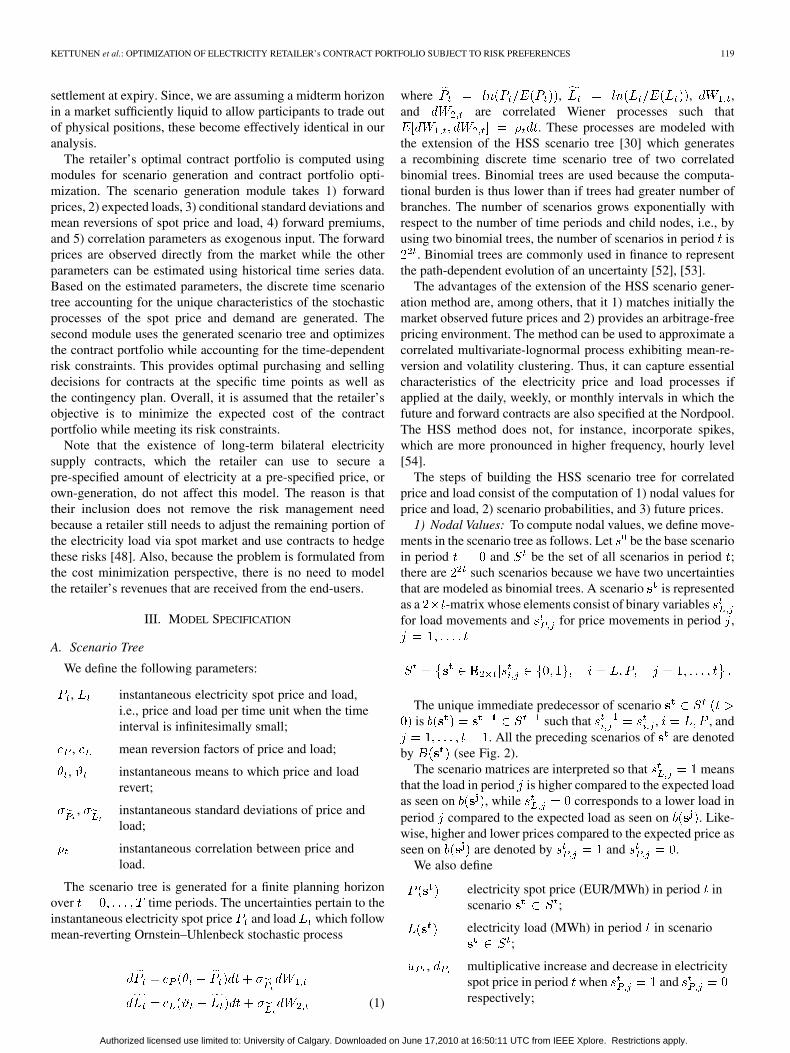
Some simplifications and adjustments were made in the ex-periments. In the scenario tree generation, probabilities of thehigher and lower prices and loads compared to the expectedlevels were rounded to obtain values between zero and one, assuggested by [28]; this is because the HSS model can, at times,result in probabilities that are either negative or greater thanone if correlation between the modeled variables is very strong[28].2 This rounding of probabilities between zero and one canmean that the tree does not match the values of the observedfutures perfectly. To avoid this, the nodal values were re-scaledafter the tree was created and a perfect match achieved (for sim-ilar approach, see [30]). Reference [30] also demonstrates thatre-scaling can be done as “the computation of the probabilitiesis independent of the means of the process” and thus the struc-ture of the stochastic process remains correct. Fig. 3 shows thescenarios in time periods and , after re-scaling. In theterminal period, , there are scenarios and theranges of values that load and price can obtain, given ,are [13.39, 19.42] and [11.57, 117.75], respectively.

Taxation issues were ignored, and it was assumed that thepurchased contracts do not influence contract prices. We also as-sumed that future contracts can be purchased in any size of units,although in reality, the minimum contract volume is 1 MW.

B. Results

The experiments were conducted to compare the mean-CCFAR efficiency of 1) our proposed stochastic optimization,2) periodic optimization, and 3) a fixed allocation strategy(in which futures were purchased according to the followingfixed percentages of the load 80%, 70%, 60%, 50%, and 40%for the one, two, three, four, and five weeks dated futures,respectively). Periodic optimization approach differs from thestochastic optimization approach by determining a single op-timal portfolio for each period instead of computing the optimal

2We observed that this phenomenon occurred also if the mean reversion pa-rameters or conditional standard deviations were high.



Fig. 3. Generated scenarios for periods � � � and � � �.

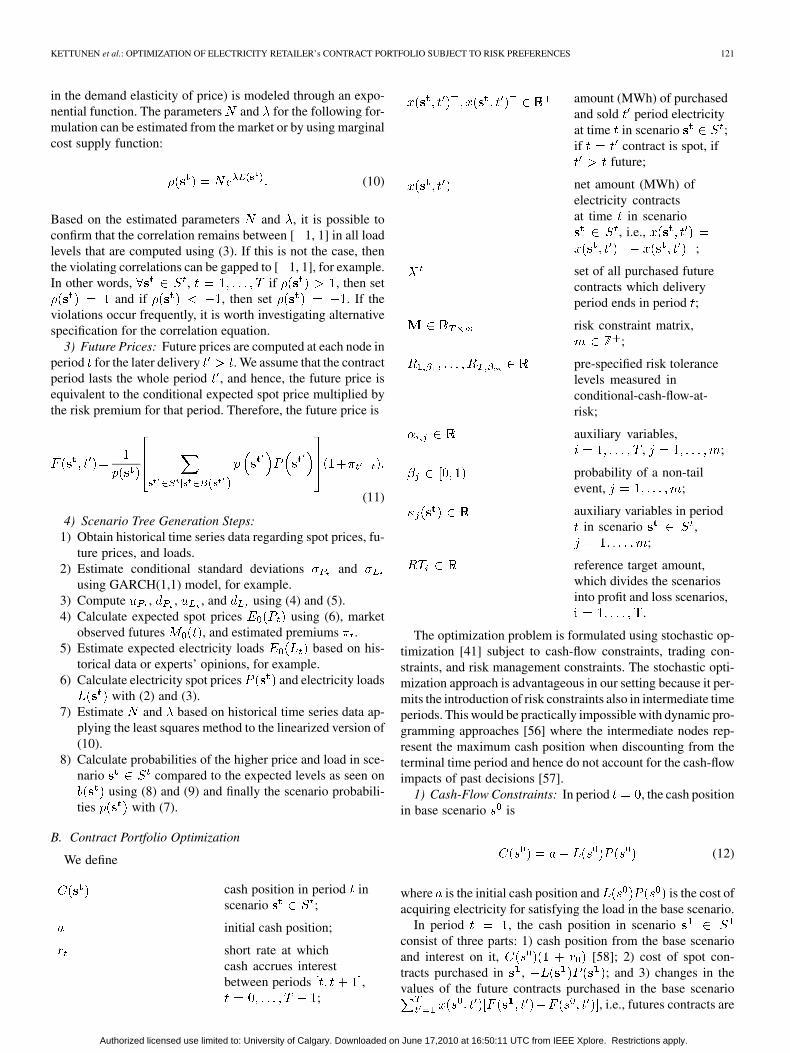
Fig. 4. Comparison of stochastic optimization, periodic optimization, and fixedallocation (figures in million EUR).

portfolio for each scenario in each period. Periodic optimiza-tion is conducted over the same scenario tree using (12)–(16)but replacing , , and with periodspecific decisions , , and , respectively.Periodic optimization approach is used, for example in MonteCarlo simulations, when the optimization is done over eachsimulation trial independently, and the decisions are averagedout for each period in the end.

Fig. 4 shows the mean-efficient frontiers with respect to thesix-week 95% CCFAR, in which losses relate to an initial budgetof 5.2 million EUR. The stochastic optimization is the most ef-ficient one with respect to the expected cost and CCFAR. For

example, a comparison of stochastic optimization with fixed al-location indicates that the same risk level (as measured by 95%CCFAR) can be attained at about 5.6% lower cost in relation tothe initial budget. The gap between the methods can be expectedto increase if the risks increase due to changes in correlation,standard deviations, or mean reversions.

From the point of view of the risk averse retailer, which cor-responds to the leftmost end of the curve, the stochastic opti-mization approach provides significant benefits in reduction ofexpected cost as contract portfolio is efficiently managed. Forthe risk neutral retailer, which corresponds to the rightmost endof the curve, the benefits of the stochastic optimization methodare less significant because only a few futures are purchased.

When the hypotheses H1–H4 were tested with respectto changes in the input parameters, these hypothesis werevalidated (see Fig. 5). Specifically, the impact of increasedpremiums can be seen in Fig. 5(a). For the risk neutral retailer(the rightmost end of the curves), the change in premiums doesnot have impact on the expected cost. In contrast, for the riskaverse retailer (the leftmost end of the curves), the increasedpremiums result in significantly higher expected cost. In fact,the impact on expected cost is stronger the more hedging isconducted.

The change in the risk (H2, H3, and H4) can be observedsimilarly by comparing the horizontal changes of the risk neu-tral retailer, for example. Fig. 5(e) and (f) shows that for theprice-related input parameters, the change in risk strongly de-pends whether the retailer is risk averse or risk neutral. Thiscan be seen by comparing the horizontal differences betweenthe curves for risk averse and risk neutral retailer. As can beseen, the risk averse retailer is almost immune to variability inprice-related input parameters while the risk can vary signifi-cantly for risk neutral retailer. Also it can be observed that un-certainty in load-related input parameters causes roughly equalamount of risk for both risk averse and risk neutral retailers[see Fig. 5(c) and (d)]. This effect can be explained by notingthat their future contracts provide a perfect hedge against pricechanges but cannot capture volume risks. Thus, both retailersneed to pay attention to the load-related uncertainties and pos-sibly use swing options to protect against the volume risks.However, the risk neutral retailer also has to be concerned aboutthe price-related risks which result in greater variability in riskthan load-related uncertainties.

Further experiments were also run with the correlation beingzero [see Fig. 5(b)] to analyze how much risk this assumptionunderestimates compared to the model with positive exponen-tial correlation. Similar tests were also run for the correlationparameter and corresponding results were obtained. The dif-ference was significant for the risk neutral retailer as risk was un-derestimated by approximately 23%, in absolute terms about 0.3million EUR, while the effect was less for risk averse retailer.Thus, including correlation into the analysis was important.

The robustness of the optimum strategies were also evaluatedby observing how close the optimal contract portfolio strategyof the original problem, i.e., solution for a given risk aver-sion, were to the efficient frontiers when the input parameterswere changed one at a time. The results suggested that theoptimal strategies of the original problem were not sensitive



Fig. 5. Sensitivity of mean-CCFAR efficient frontier with respect to changes in (a) �, (b) N, (c) � , (d) � , (e) � , and (f) � .

Note, the change in premiums corresponded to the change in the gradient and in conditional standard deviations to a parallel shift.

to the changes in the input parameters. These are illustratedalso in Fig. 5. Here the point marked with “O” is the optimalcontract portfolio strategy of the original problem, when sixweek CCFAR constraint was set to 0.4 million EUR, and isthus on the mean-CCFAR efficient frontier. The points marked

with “X” are computed applying the original contract portfoliostrategy when the input parameter was 50%3 higher and lower,respectively, than originally.

3For N, we used 20% as an increase of 50% would have resulted correlationvalues that were greater than 1.



Fig. 6. Mean efficient surface with respect to four weeks and six weeks 95%CCFAR (figures in million EUR).

Finally, we conducted experiments to analyze the effects ofintroducing a risk constraint matrix (with two risk constraints)compared to a single risk constraint. For this purpose, we plotthe mean-CCFAR efficient surface with respect to four and sixweeks 95% CCFAR, which losses relate to an budget of 3.5and 5.2 million EUR, respectively (see Fig. 6). The risk neutralretailer is located in this graph close to the corner marked asat which point the cost of the portfolio is minimized. The riskaverse retailer is close to the extreme corners in the opposite end,for example at point marked as , depending on the requiredlevel of risks at six and four weeks.

In Fig. 6, we also highlight a point A which represents a sit-uation when the expected procurement costs are minimized anda risk constraint only on the six weeks 95% CCFAR is appliedat the level of 0.6 million EUR. At this point, the risk at theintermediate four weeks 95% CCFAR is not curtailed. How-ever, by setting an additional constraint for the four weeks 95%CCFAR at the level of 0.4 million EUR, it is possible to reducethe four weeks risk by approximately 50% (in absolute termsroughly 0.5 million EUR) while the increase in cost is insignif-icant being only by 0.1% (in absolute terms only 0.005 millionEUR). Consequently, setting constraints concurrently at severaltime periods can reduce significantly the intermediate periodrisks which can be important, for example due to regulatory rea-sons or if the company is close to financial distress.

V. CONCLUSIONS

Our results suggest that the stochastic optimization approachcan be more efficient for risk management by an electricity re-tailer than periodic optimization or fixed allocation approaches.This result can be attributed to the fact stochastic optimizationuses the path dependency of information along individual sce-nario paths to optimize hedging in each period. This result isalso analogous to the findings of [6] which compares the effec-tiveness of a production and hedging portfolio using dynamicand static models for electricity production.

One of the key insights from the numerical studies is that it isimportant to incorporate the correlation between spot price and

load into the model as correlation increases the probability ofthe extreme outcomes and hence risks. The results of the exper-iments also suggest that a risk neutral retailer would be moreconcerned about the price-related uncertainties, which resultin greater variability in risk, than load related uncertainties. Arisk averse retailer, on the other hand, should estimate carefullythe risk premiums which strongly affect the expected cost andshould also use derivatives, such as swing contracts, to hedge forload-related uncertainties. Overall the model is relatively robustin that the solutions remain close to the efficient frontier even ifthere are minor variations in the input parameters.

Our approach also includes CCFAR constraints across severaltime periods rather than focusing only upon the terminal period.This is important as it allows retailers to keep the cash position inintermediate periods within risk limits for satisfying complianceregulation requirements or above a desired risk level if the com-pany is financially constrained. This risk management across in-termediate periods is also important in the methodology, as re-tailers will continue to operate after the terminal period, and inpractice, risk management needs to feed forward continuously.Consequently, it is important in practice to incorporate the risksduring the intermediate time periods and to re-run the model forall time periods, rolling forward, when updated information be-comes available. The same rationale applies to risk managementat different confidence levels, as well.

This research has made contributions to the general direc-tion of methodology. It is possible to integrate additional details,for instance regarding the special market characteristics of theprice formation process and load prediction errors, to considerdifferent time specifications, as well as cross-hedging with re-lated markets, most of which present substantial but essentiallycomputational extensions. But, more generally, this research hasdemonstrated that more accurate results can be achieved in theelectricity retailing business by incorporating path-dependen-cies in the generated scenarios and using multistage evaluationto optimize hedging at intermediate stages. We found that sto-chastic optimization, combined with a risk constraint matrixframework and allied to the HSS scenario building process, pro-vided a viable methodology for this class of problems. Further-more, it provides insights into the relative sensitivity of riskmanagement parameters to different kinds of market partici-pants in this context.

ACKNOWLEDGMENT

The authors would like to thank S. Makkonen for fruitful dis-cussions and K. Berg, A. Toppila, and E. Vilkkumaa for com-ments on the previous versions.

REFERENCES

[1] C. J. Andrews, “Evaluating risk management strategies in resourceplanning,” IEEE Trans. Power Syst., vol. 10, no. 1, pp. 420–426, Feb.1995.

[2] R. Dahlgren, C.-C. Liu, and J. Lawarree, “Risk assessment in energytrading,” IEEE Trans. Power Syst., vol. 18, no. 2, pp. 503–511, May2003.

[3] B. Mo, A. Gjelsvik, and A. Grundt, “Integrated risk managementof hydro power scheduling and contract management,” IEEE Trans.Power Syst., vol. 16, no. 2, pp. 216–221, May 2001.

[4] A. J. Conejo, J. M. Arroyo, J. Contreras, and F. A. Villamor, “Self-scheduling of a hydro producer in a pool-based electricity market,”IEEE Trans. Power Syst., vol. 17, no. 4, pp. 1265–1272, Nov. 2002.



[5] E. Ni, P. B. Luh, and S. Rourke, “Optimal integrated generation bid-ding and scheduling with risk management under a deregulated powermarket,” IEEE Trans. Power Syst., vol. 19, no. 1, pp. 600–609, Feb.2004.

[6] S.-E. Fleten, S. W. Wallace, and W. T. Ziemba, “Hedging electricityportfolios via stochastic programming,” in Decision Making UnderUncertainty: Energy and Power. IMA Volumes in Mathematics andIts Applications, C. Greengard and A. Ruszczynski, Eds. New York:Springer-Verlag, 2002, pp. 71–93.

[7] I. Vehviläinen and J. Keppo, “Managing electricity market price risk,”Eur. J. Oper. Res., vol. 145, no. 1, pp. 136–147, 2003.

[8] S. Makkonen, “Decision modelling tools for utilities in the deregu-lated energy market” Dr.Tech. dissertation, Helsinki Univ. Technol.,Helsinki, Finland, 2005 [Online]. Available: http://www.tkk.fi/Eng-lish/, Systems Analysis Laboratory Research Report A93.

[9] M. Liu and F. F. Wu, “Managing price risk in a multimarket environ-ment,” IEEE Trans. Power Syst., vol. 21, no. 4, pp. 1512–1519, Nov.2006.

[10] M. Denton, A. Palmer, A. Masiello, and P. Skantze, “Managing marketrisk in energy,” IEEE Trans. Power Syst., vol. 18, no. 2, pp. 494–502,May 2003.

[11] D. W. Bunn, Modelling Prices in Competitive Electricity Markets.London, U.K.: Wiley, 2004.

[12] S. Takriti, B. Krasenbrink, and L. S.-Y. Wu, “Incorporating fuel con-straints and electricity spot prices into the stochastic unit commitmentproblem,” Oper. Res., vol. 48, no. 2, pp. 268–280, 2000.

[13] J. Doege, P. Schiltknecht, and H.-J. Lüthi, “Risk management of powerportfolios and valuation of flexibility,” OR Spectr., vol. 28, no. 2, pp.1–21, 2006.

[14] M. Burger, B. Klar, A. Müller, and G. Schindlmayr, “A spot marketmodel for pricing derivatives in electricity markets,” Quant. Fin., vol.4, no. 1, pp. 109–122, 2004.

[15] A. Eichhorn, N. Gröwe-Kuska, A. Liebscher, W. Römisch, G. Span-gardt, and I. Wegner, “Mean-risk optimization of electricity portfolios,”in Proc. PAMM Applied Mathematics and Mechanics Minisymp. MA1,2004, vol. 4, no. 1, pp. 3–6. [Online]. Available: http://www3.inter-science.wiley.com/.

[16] H. Heitsch and W. Römisch, “Scenario reduction algorithms in sto-chastic programming,” Comput. Optim. Appl., vol. 24, no. 2–3, pp.187–206, 2003.

[17] L. Clewlow and C. Strickland, Valuing Energy Options in a One FactorModel Fitted to Forward Prices 1999, working paper, Univ. Sydney.[Online]. Available: http://www.ssrn.com/abstract=160608.

[18] L. Clewlow and C. Strickland, Energy Derivatives: Pricing and RiskManagement. London, U.K.: Lacima, 2000.

[19] S. Koekebakker and F. Ollmar, “Forward curve dynamics in the Nordicelectricity market,” Manag. Fin., vol. 31, no. 6, pp. 73–94, 2005.

[20] M. Manoliu and S. Tompaidis, “Energy futures prices: Term structuremodels with Kalman filter estimation,” Appl. Math. Fin., vol. 9, no. 1,pp. 21–43, 2002.

[21] F. E. Benth, L. Ekeland, R. Hauge, and B. R. F. Nielsen, “A note onarbitrage-free pricing of forward contracts in energy markets,” Appl.Math. Fin., vol. 10, no. 4, pp. 325–336, 2003.

[22] N. Gröwe-Kuska, H. Heitsch, and W. Römisch, “Scenario reductionand scenario tree construction for power management problems,”in Proc. 2003 IEEE Bologna Power Tech Conf., 2003, vol. 3. [On-line]. Available: http://www.ieeexplore.ieee.org/xpl/abs_free.jsp?ar-Number=1304379.

[23] T. Pennanen, “Epi-convergent discretizations of multistage stochasticprograms,” Math. Oper. Res., vol. 30, no. 1, pp. 245–256, 2005.

[24] J. Dupacova, G. Consigli, and S. W. Wallace, “Scenarios for multistagestochastic programs,” Ann. Oper. Res., vol. 100, no. 1–4, pp. 25–53,2000.

[25] K. Høyland and S. W. Wallace, “Generating scenario trees for multi-stage decision problems,” Manage. Sci., vol. 47, no. 2, pp. 295–307,2001.

[26] R. Kouwenberg, “Scenario generation and stochastic programmingmodels for asset liability management,” Eur. J. Oper. Res., vol. 134,no. 2, pp. 279–292, 2001.

[27] G. Pflug, “Scenario tree generation for multiperiod financial optimiza-tion by optimal discretization,” Math. Program. Fin., vol. 89, no. 2, pp.251–271, 2001.

[28] T.-S. Ho, R. C. Stapleton, and M. G. Subrahmanyam, “Multivariatebinomial approximations for asset prices with nonstationary varianceand covariance characteristics,” Rev. Fin. Stud., vol. 8, no. 4, pp.1125–1152, 1995.

[29] T. S. Ho, R. C. Stapleton, and M. G. Subrahmanyam, “The risk ofa currency swap: A multivariate-binomial methodology,” Eur. Fin.Manage., vol. 4, no. 1, pp. 9–27, 1998.

[30] S. J. Peterson and R. C. Stapleton, “The pricing of Bermudan-style op-tions on correlated assets,” Rev. Deriv. Res., vol. 5, no. 2, pp. 127–151,2002.

[31] Risk Management, 2009. [Online]. Available: http://www.riskmetrics.com.

[32] G. Szegö, “Measures of risk,” J. Bank. Fin., vol. 26, no. 7, pp.1253–1272, 2002.

[33] G. J. Alexander and A. M. Baptista, “Economic implications ofusing a mean-VAR model for portfolio selection: A comparison withmean-variance analysis,” J. Econ. Dynam. Control, vol. 26, no. 7–8,pp. 1159–1193, 2002.

[34] P. Embrechts, S. I. Resnick, and G. Samorodnitsky, “Extreme valuetheory as a risk management tool,” North Amer. Actuarial J., vol. 3,no. 2, pp. 30–41, 1999.

[35] S. Uryasev, “Introduction to the theory of probabilistic functions andpercentiles (value-at-risk),” in Probabilistic Constrained Optimiza-tion: Methodology and Applications, S. Uryasev, Ed. Norwell, MA:Kluwer, 2000, pp. 1–25.

[36] J. Danielsson, P. Embrechts, C. Goodhart, C. Keating, F. Muennich, O.Renault, and H.-S. Shin, An Academic Response to Basel II, SpecialPaper No. 130, FMG ESRC, 2001. [Online]. Available: http://www.riskresearch.org.

[37] R. T. Rockafeller and S. Uryasev, “Optimization of conditionalvalue-at-risk,” J. Risk, vol. 2, no. 3, pp. 21–41, 2000.

[38] A. Eichhorn, W. Römisch, and I. Wegner, “Polyhedral risk measuresin electricity portfolio optimization,” in Proc. PAMM Applied Mathe-matics and Mechanics Minisymp. MA1, 2004, vol. 4, no. 1, pp. 7–10.[Online]. Available: http://www3.interscience.wiley.com/.

[39] J. Cabero, A. Barillo, S. Cerisola, M. Ventosa, A. Garcia-Alcalde, F.Peran, and G. Relano, “A medium-term integrated risk managementmodel for a hydrotermal generation company,” IEEE Trans. PowerSyst., vol. 20, no. 3, pp. 1379–1388, Aug. 2005.

[40] R. A. Jabr, “Robust self-scheduling under price uncertainty using con-ditional value-at-risk,” IEEE Trans. Power Syst., vol. 20, no. 4, pp.1852–1858, Nov. 2005.

[41] J. R. Birge and F. Louveaux, Introduction to Stochastic Program-ming. New York: Springer, 1997.

[42] S. Sen, L. Yu, and T. Genc, “A stochastic programming approach topower portfolio optimization,” Oper. Res., vol. 54, no. 1, pp. 55–72,2006.

[43] K. Frauendorfer and J. Güssow, “Stochastic multistage programming inthe operation and management of a power system,” in Stochastic Opti-mization Techniques (Neubiberg/Munich, 2000), C. Greengard and A.Ruszczynski, Eds. Berlin, Germany: Springer, 2002, vol. 513, Lec-ture Notes in Economics and Mathematical Systems, pp. 199–222.

[44] A. J. Conejo, R. García-Bertrand, M. Carrión, A. Caballero, and A. deAndrés, “Optimal involvement in futures markets of a power producer,”IEEE Trans. Power Syst., vol. 23, no. 2, pp. 703–711, May 2008.

[45] S. Pineda, A. J. Conejo, and M. Carrión, “Impact of unit failure onforward contracting,” IEEE Trans. Power Syst., vol. 23, no. 4, pp.1768–1775, Nov. 2008.

[46] M. Carrión, A. J. Conejo, and J. M. Arroyo, “Forward contracting andselling price determination for a retailer,” IEEE Trans. Power Syst., vol.22, no. 4, pp. 2105–2114, Nov. 2007.

[47] S. A. Gabriel, M. F. Genc, and S. Balakrishnan, “A simulation approachto balancing annual risk and reward in retail electrical power markets,”IEEE Trans. Power Syst., vol. 17, no. 4, pp. 1050–1057, Nov. 2002.

[48] S. A. Gabriel, A. J. Conejo, M. A. Plazas, and S. Balakrishnan, “Op-timal price and quantity determination for retail electric power con-tracts,” IEEE Trans. Power Syst., vol. 21, no. 1, pp. 180–187, Feb. 2006.

[49] S.-E. Fleten and E. Pettersen, “Constructing bidding curves for a price-taking retailer in the norwegian electricity market,” IEEE Trans. PowerSyst., vol. 20, no. 2, pp. 701–708, May 2005.

[50] P. Skantze, M. Ilic, and J. Chapman, “Stochastic modeling of electricpower prices in a multi-market environment,” in Proc. IEEE PowerEng. Soc. Winter Meeting, 2000, vol. 2, pp. 1109–1114.

[51] T. Kristiansen, “Pricing of contracts for difference in the Nordicmarket,” Energy Pol., vol. 32, no. 9, pp. 1075–1085, 2004.

[52] J. C. Cox, S. A. Ross, and M. Rubinstein, “Option pricing: A simplifiedapproach,” J. Fin. Econ., vol. 7, no. 3, pp. 229–263, 1979.

[53] F. Black, E. Derman, and W. Toy, “A one-factor model of interest ratesand its application to treasury bond options,” Fin. Anal. J., vol. 46, no.1, pp. 33–39, 1990.

[54] F. A. Longstaff and A. W. Wang, “Electricity forward prices: A high-frequency empirical analysis,” J. Fin., vol. 59, no. 4, pp. 1877–1900,2004.

[55] H. Shawky, A. Marathe, and C. Barrett, “A first look at the empirical re-lation between spot and futures electricity prices in the United States,”J. Futures Markets, vol. 23, no. 10, pp. 931–955, 2003.



[56] D. P. Bertsekas, Dynamic Programming and Optimal Control Volume1. Belmont, CA: Athena Scientific, 1995.

[57] P. Krokhmal and S. Uryasev, “A sample-path approach to optimal po-sition liquidation,” Ann. Oper. Res., vol. 152, no. 1, pp. 1–33, 2007.

[58] J. Gustafsson and A. Salo, “Contingent portfolio programming for themanagement of risky projects,” Oper. Res., vol. 53, no. 6, pp. 946–956,2005.

[59] P. Artzner, F. Delbaen, J.-M. Eber, and D. Heath, “Coherent measuresof risk,” Math. Fin., vol. 9, no. 3, pp. 203–228, 1999.

[60] F. Delbaen, Coherent Risk Measures on General Probability Spaces,eTH Zürich, 2000. [Online]. Available: http://www.actuaries.org/AFIR/colloquia/Tokyo/Delbaen.pdf, Tech. Rep.

[61] I. Rasool, H. Crump, and V. Munerati, Liquidity in the GB Whole-sale Energy Markets, Office of Gas and Electricity Markets, DiscussionPaper 62/09, 2009.

[62] A. Cartea and P. Villaplana, “Spot price modeling and the valuationof electricity forward contracts: The role of demand and capacity,” J.Bank. Fin., vol. 32, no. 12, pp. 2502–2519, 2008.

[63] Energiateollisuus, Electricity Netproduction, Imports and Exports(GWh) in Finland, 2006. [Online]. Available: http://www.energia.fi.

Janne Kettunen (M’08) is an Assistant Professor atthe University of Calgary, Calgary, AB, Canada. Hisresearch interests are focused on the decision analyticmodeling of investment under market uncertainties,specifically in the contexts of electricity and carbonmarkets.

Prof. Kettunen was one of the four finalists inDennis J. O’Brien United States Association forEnergy Economics Best Student Paper Competitionwith the paper “Electricity investment behavior inresponse to climate policy risk” in December 2008.

Ahti Salo received the M.Sc. and Dr.Tech. de-grees from the Helsinki University of Technology,Helsinki, Finland, in 1987 and 1992, respectively.

He is a Professor of systems analysis at the Sys-tems Analysis Laboratory of the Helsinki Universityof Technology. His current research interests includetopics in portfolio decision analysis, multi-criteriadecision making, risk management, efficiencyanalysis, and technology foresight. He has beenresponsible for the development and deployment ofmethodological support for numerous high-impact

decision and policy processes, including FinnSight 2015, the national foresightexercise of the Academy of Finland and the Finnish Funding Agency forTechnology and Innovation (Tekes).

Derek W. Bunn is a Professor at the LondonBusiness School, London, U.K., with research on theenergy sector extending back over 30 years. He is theauthor of numerous research papers and books in theareas of forecasting, decision analysis, and energyeconomics. He has advised many internationalcompanies and government agencies in this sector.

Prof. Bunn has been the Editor of the Journal ofForecasting since 1984, a previous Editor of EnergyEconomics, and Founding Editor of the new Journalof Energy Markets.


Documents

Optimization of Electricity Retailer’s Contract Portfolio