Optimization of 2D boundary element models using -splines ... · of GAs with geometric modeling, by using b-splines curves, in order to solve non-conventional problems like shape

Optimization of 2D boundary element models usingb-splines and geneticalgorithms

M. Cerrolazaa,* , W. Annicchiaricoa, M. Martinezb

aInstitute for Materials and Structural Models, Faculty of Engineering, Central University of Venezuela, PO Box 50.361, Caracas 1050-A, VenezuelabSchool of Mechanical Engineering, Faculty of Engineering, Central University of Venezuela, Caracas 1050-A, Venezuela

Received 29 April 1999; received in revised form 7 October 1999; accepted 15 February 2000

Abstract

The optimization of bidimensional shapes is one of the most commonly addressed problems in engineering. This work is concerned withthe use of Genetic Algorithms (GAs) andb-spline-curves modeling for the optimization of Boundary Element Models (BEM). The paperbriefly summarizes the basis of the GAs formulation and describes how to use refined genetic operators. The model boundary is discretizedby using the BEM, and selected parts of the boundary are modeled by usingb-spline curves, in order to allow easy remeshing and adaptationof the boundary to the external actions. Two numerical examples are presented and discussed in detail, showing that the proposed combinedtechnique is able to optimize the shape of the domains with minimum computational effort. The reduction in the model area is significant,without violating the restrictions imposed to the model.q 2000 Elsevier Science Ltd. All rights reserved.

Keywords: S shape optimization; Genetic algorithms;b-Splines modeling

1. Introduction

Shape optimization of continuum models is a subject ofconcern to design engineers. For a long time, this field ofresearch has deserved great attention from the numericalanalysis community and many available optimization tech-niques have been developed and successfully used in engi-neering analysis and design. In this class of problems,aspects such as geometric definitions, mesh generation,analysis and displaying of results are usually involved.Furthermore, other elements play a decisive role in the opti-mization process, such as sensitivity analysis and numericaloptimization programming.

The problem can be divided into three main tasks. Thefirst step is to define the geometric and the analyticalmodels. The geometric model is where the design variablesare easily imposed and it allows an explicit integration withother design tools, such as CAD or CAM systems. On theother hand, the analytical model is used to obtain the struc-tural response of the part, subjected to external actions.Then, a sensitivity analysis must be done to obtain a solutionof the problem; and finally, an appropriate optimization

algorithm must be selected to solve the optimizationproblem in an effective and reliable way.

Since Zienkiewicz and Campbell [1] initiated the numer-ical treatment of shape optimization problems, a largenumber of publications have appeared in the field of shapesensitivity analysis. Haug et al. [2] presented a unifiedtheory of continuum shape design sensitivity using a varia-tional formulation for the governing equations of structuralmechanics and material derivative concepts. Severalresearches, see for instance Yang and Botkin, and Yaoand Choi [3,4] who have investigated the accuracy of theshape design sensitivity theory utilizing the finite elementmethod (FEM) because of its variational formulation.Generally, the shape design sensitivity formula requiresthe evaluation of accurate stress quantities on the boundary,which is usually difficult to obtain by the FEM. The Bound-ary Element Method has become a popular alternative inshape design sensitivity analysis due to its accuracy of theboundary displacement and stress solutions as well as thefact that remeshing is easier for the BEM than for the FEM.The evaluation of design sensitivities are the adjoin methodand direct differentiation method. The reader can find manyworks in the technical literature on this subject. Choi andKwak, Baron and Yang, Kane and Saigal, Mellings andAliabadi, and Mellings [5–9], have presented numericalresults in the optimization of potential and two-dimensional(2D) elasticity problems. Also, Meric [10] presented a

Engineering Analysis with Boundary Elements 24 (2000) 427–440

0955-7997/00/$ - see front matterq 2000 Elsevier Science Ltd. All rights reserved.PII: S0955-7997(00)00006-0

www.elsevier.com/locate/enganabound

* Corresponding author.E-mail addresses:[email protected] (M. Cerrolaza), annwill@

sagi.ucv.edu.ve (W. Annicchiarico).

sensitivity analysis of 2D shape optimization with BEM,comparing integral and differential formulations in heatconduction problems. Another work by Parvizian andFenner [11] optimizes 2D boundary element models usingmathematical programming and normal movementtechniques.

The recent paper of Kita and Tanie [12] proposed anapproach based on Genetic Algorithms (GAs) and BEM,where the initial mesh is set up with a rectangular mesh ofnodes. These nodes move their position, following geneticoptimization, until the optimal shape is reached. The resultsare encouraging although the user cannot define an initialreal mesh.

Initially, some authors such as Zienkiewicz and Camp-bell, and Ramakrishnan and Francavilla [1,13] amongothers, did not use geometric modeling in the shape optimi-zation problems addressed by them. Instead, they definedthe nodal coordinates of the discrete FEM as design vari-ables. This approach has limitations such as:

1. it requires a large number of design variables and tends toproduce jagged-edges shapes;

2. a large number of constraints must be added in order togenerate smooth boundaries, which complicates thedesign task;

3. the lack of an associated geometric model does not allowthe integration with powerful design tools like CAD orCAM systems.

The success of any optimization methodology hinges onits ability to deal with complex problems, as is the case ofshape optimization design. Solving non-linear optimizationproblems efficiently is challenging. Furthermore, it is quitecommon in practice that methods are modified, combinedand extended in order to construct an algorithm that matchesbest the features of the particular problem at hand. For thesereasons, emphasis has to be made on the basis of variousmethods in order to choose the most appropriate.

The search for a robust optimization algorithm, with goodbalance between efficiency and efficacy, necessary tosurvive in many different environments, has led to the useof GAs. GAs have many advantages over traditional search-ing methods. Among other considerations, they do not needfurther additional information than objective functionvalues or fitness information. This information is used todetermine the success or failure of a design in a particularenvironment. Moreover, its ability to find out the optimumor quasi-optimum solution gives it a privileged position as apowerful tool in non-conventional optimization problems.All of these advantages have led to propose the combinationof GAs with geometric modeling, by usingb-splines curves,in order to solve non-conventional problems like shape opti-mization problems.

In CAD systems, the geometric modeling is carried out byusing Lagrange polynomials, Bezier curves, B-splines andb-splines curves and surfaces as well as coons patches (seefor instance, Refs. [14–16]). Among these approaches, the

b-spline curve properties can be easily controlled by usingits parameters. Other advantages that encourage the use ofthis technique are:

• the curve lies in a convex hull of the vertices;• the curve does not depend on an affine-transformation;• the tangents of the initial and final points are defined

respectively by the first and the last edge of the polygon.The above characteristic allows the imposition of C1

continuity [14].

In previous works [17,18] it has been shown that GAsprovide a powerful tool to optimize bidimensional FEmodels. However, the use of nodal coordinates in the FEmodel has proven to be somewhat difficult to control, whichsuggested the use of a class of spline-curves to model theboundary variation.

Thus, recent developments by the authors in shape opti-mization using the FEM andb-spline curves [19,20],suggested the extension of some of the ideas previouslypresented to their application to the genetic optimizationof bidimensional engineering problems discretized by theBEM.

2. A review of GAs formulation

This section is devoted to give the reader a brief reviewon how GAs work. A detailed GAs formulation can befound in the works of Holland, Goldberg and Davis [21–23], among others.

The first step in finding out the best design consists in thedefinition of the basic characteristics of the final product thatwill be optimized. These features could be the size, thick-ness, shape or topological configuration of their compo-nents. In GAs, a particular design (A) is represented by aset of its characteristicsai, called phenotype and defined asreal numbers

The phenotype of a structure is formed by the interactionof the total package with

A� a1 p a2 p a3 p …p ac �Yc

i�1

ai ai [ R �1�

its environment and its genotype is obtained by encodingeach ai into a particular code (binary in this case). Thetransformation of the phenotype structure into a string ofbits leads to the so-calledchromosomes, and it represents,like in natural systems, the total genetic prescription for theconstruction and operation of some organism

A�Yc

i�1

ai �Yc

i�1

�e : ai ! {0 ;1}� �2�

GAs operate on populations of strings (structures) andprogressively�t � 0;1;2…� modifies their genotypes toobtain the best performance of their phenotype environmentE.

M. Cerrolaza et al. / Engineering Analysis with Boundary Elements 24 (2000) 427–440428

The adaptation process is based on the mechanics ofnatural selection and natural genetics. They combine thesurvival of the fittest together with string structures, with astructured yet randomized information, which is exchangedto form a search algorithm. In each generation, using bitsand pieces of the fittest of the previous generation generatesa new set of artificial creatures (strings). They efficientlyexploit already known information to speculate on newsearch points with expected improved performance.

In order to use GAs it is necessary to define an objectivefunction or fitness function that measures the behavior ofeach individual into its environment. This function providesa direct indication of the performance of each individual tosolve the optimization problem subjected to the imposedconstraints of the environment. With this population rankedaccording to fitness, a group of chromosomes are selectedfrom the population. There exist several methods to chooseparents. In this work, the following methods have been used[17]:

• Stochastic sampling with replacement (SSWR), in thismethod the selection probability of an individual isproportional to its fitness value. So that, individualswith high fitness (above mean population fitness) willsurely have an increasing number of copies, individualswith average fitness stay even and individuals with lowfitness will have a decreasing number of copies in thenext generation and eventually die off.

• Remainder stochastic sampling without replacement(RSSWR) is a scheme where the probabilities of selec-tion are calculated as usual, pselecti � fi =Sf : Then theexpected number of individuals for each stringei is calcu-lated asei � pselecti p n: Each string allocates samplesaccording to the integer part ofei values. The fractionalpart ofei is treated as success probabilities to give morecopies in the next generation.

The selected chromosomes are then reproduced throughthe crossover and mutation operators. The crossover opera-tor consists in taking two selected chromosomes as parents.Then, they are either crossed by using a certain probabilityvalue in order to create two new chromosomes (‘children’)or they are directly included into the new population. In thepresent implementation of GAs, there are no specialschemes for saving the birth of individuals with low func-tion evaluation. They could be born but they are finallyremoved from the population by the mechanics of the survi-val of the fittest.

Many procedures can be found in the technical literature[24] to carry out the reproduction operation. In the presentwork the following can be used: one break point (simplecrossover), two break-points (double crossover) anduniform crossover, since these methods lead to a simpleand reliable solutions (see Fig. 1).

In simple crossover, an integer positionn1 along the stringis randomly chosen between 1 and the string length less one

[1,1 2 1]. Then, two new strings are created by swapping allthe characters between positionn1 1 1 and 1.

The two break points method is based on the interchangeof the sub-string placed between bitsn1 and n2 of theparents. Both numbers are randomly chosen, in the sameway as simple crossover.

Uniform crossover method consists in generating twonew children in the following way: the genes of the firstchild are made by the parent genes chosen with the prob-ability of the crossover patron and the genes of the secondchild with the contrary. The crossover patron is generated inorder to find the same probability of selection for the genesof each parent, as shown in Fig. 1.

The normal mutation operator gives each bit in a chromo-some the opportunity of changing (if it is 1 to 0 or viceversa).

The selection according to the fitness, combined with thecrossover, provides GAs the bulk of their processing power.Mutation plays a secondary role in the operation of the GAsand it is needed because, even though selection and cross-over effectively search and recombine extant notions, occa-sionally they may become overzealous and they can losesome potentially useful genetic material (1’s or 0’s at parti-cular locations). Thus, the normal mutation operator protectsagainst such an irrecoverable premature loss of importantnotions. Owing to the secondary importance of this operator,a low mutation probability value is usually considered.

What is the power involved behind these simple transfor-mation over a random population ofn strings, that allowgenetics algorithms to find the optimum point (or nearly theoptimum point) in complex and non-linear situations? Theanswer of this question was found by John Holland and it isexposed in the ‘Schema Theorem’ or ‘The FundamentalTheorem of Genetic Algorithms [21].

A schema is a similarity template describing a subset ofstring displaying similarities at certain string positions. It isformed by the ternary alphabet {0.1,p }, where p is simplya notational symbol, that allows the description of all possi-ble similarities among strings of a particular length andalphabet. In general, there are 21 different strings or chro-mosomes of length 1, but schemata display an order of 31. Aparticular string of length 1 inside a population ofn indivi-duals into one of the 21 schemata can be obtained from thisstring. Thus, in the entire population the number of sche-mata present in each generation is somewhere between 21

andn21, depending upon the population diversity. But, howmany of them are processed in a useful way? Clearly, not allof them have the same possibility to carry on its geneticinformation through each generation, since genetic opera-tors could destroy some of them. Holland estimated that in apopulation ofn chromosomes, the GAs processO(n3) sche-mata into each generation. He named this as ‘Implicit Paral-lel Process’.

Even though at each generation are performed a propor-tional computation to the size of the populationn, the algo-rithm carries out a more efficient process on then3 schemata

M. Cerrolaza et al. / Engineering Analysis with Boundary Elements 24 (2000) 427–440 429

with no further information than that contained into thepopulation itself. Holland has shown that ‘good schemata’,mainly related to high fitness values, are propagated genera-tion to generation by giving exponentially increasingsamples to the observed best; and bad schemata disappear.At the end of the generation process, the chromosomes inthe population are only formed from good schemata, whichhe called ‘Building Blocks’.

2.1. Some refined operators

There exist several new operators [17,23] that can be usedtogether with the basic reproduction, crossover andmutation operators, explained before. In the presentwork, two refined operators, called rebirth and elitism, areused to improve the results obtained with a simple geneticalgorithm.

2.1.1. RebirthRebirth is not really a genetic operator, because it does

not work directly over the chromosome [25]. This operatorworks over the procedure to obtain the best chromosomes.The basic idea of this operator is to obtain a good fit, in order

to get the desired optimum. Genetic algorithm is a stochasticand dynamic search process, which achieves a near optimalsolution of the objective scalar function in every evaluation.This near optimal solution means:

uOi 2 ObjuOi

# ek; 0 # ek p 1; k � 1;2;…; ne �3�

whereOI is the ideal objective scalar function,Obj the bestobjective scalar function in runj, ne the number of runs.Also in the phenotype structure:

uIk 2 bjk uIk

# ek; 0 # ek p 1; k � 1; 2;…;nc �4�

whereIk is the phenotypek of the ideal chromosomeI, bjk

the phenotypek of the best chromosome in the processj, ncthe number of chromosomes.

When the genetic algorithm converges to the near optimalsolution, the process is stopped and it is made the ‘rebirth’ ofa new population, thus creating random chromosomes in asubspace of the initial phenotype space. This subspace isdefined by taking a range of variation (r) for each pheno-type, which is less than the one used during the initial step,


Fig. 1. Different crossover schemes.

and by taking the best last value obtained before rebirth asthe starting of the interval for each new chromosome. So, ifP is the best last chromosome, then the new phenotypestructures are bound in the following way:

Pi 2 r # ai # Pi 1 r i � 1;2;…; nc �5�In this way, it is possible to fit the searching of the opti-

mum, because a new process is started with a new randompopulation created into a reduced phenotypic space of thebest chromosomes belonging to the initial step.

2.1.2. ElitismThe operations of crossover and mutation can affect the

best member of the population, giving no offspring into thenext generation. The elitist strategy [23] fixes this potentialsource of losing by copying the best member of eachgeneration into the succeeding generation. The elitist strat-egy may increase the domination speed exerted by a super-individual on the population. However, it seems to improvethe genetic algorithm performance.

3. Boundary element modeling usingb-spline curves

The b-spline curves are geometric design elements,which stem from the well-known B-spline curves. Thisformulation [26–28] defines additional parameters thatcontrol the bias (b1) and tension (b2) of each curve segment.The effect of these parameters is to change the parametriccontinuity between the curve segments while maintainingthe geometric continuity.

The parametric equations ofb-splines can be visualizedas the path of a particle moving through space. Increasingb1 above unity, the velocity of the particle immediatelyafter a knot point increases. This serves to push it furtherin the direction of travel before it turns as influenced by the

next control point. This is said to bias the curve to the right.Decreasingb1 below unity, the particle velocity decreasesand thus, it biases the path towards the left. The parameterb2 controls the tension in the curve. Asb2 is increasedabove zero, the knot points are pulled towards their respec-tive control points. For negativeb2, the knot points arepushed away. There are two types of formulation:

• uniformly shapedb-splines, where the parametersb1 andb2 have the same value along the entire curve;

• continuously shapedb-splines, whereb1 andb2 can havedifferent values along the different curve segments.

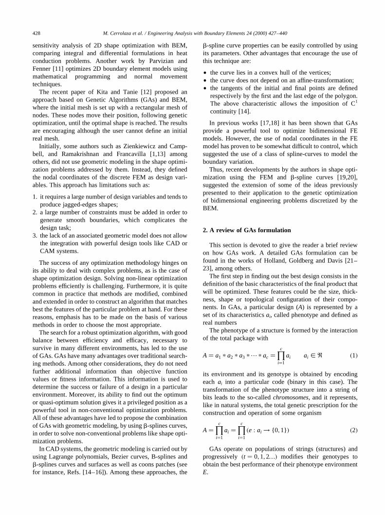
Theb-spline curves are defined with a set of points calledcontrol vertices (Vm). Although these points are not part ofthe generated curve, they completely define its shape. Thevertices of a curve are sequentially ordered and connected insuccession to form a control polygon (see Fig. 2). In thisway, theb-spline curve approximates a series ofm1 1control vertices with m parametric curve segments,Qi(u).The coordinates of a pointQi(u) on thei th curve segment arethen given by

Qi�u� �X1

r�2 2

br �b1;b2; u�Vi1r

0 # u , 1 i � 0…m2 1 �6�One of the most important advantages of this formulation

is local control. This control is obtained by using the piece-wise representation of theb-splines formulation, which isbased in a local basis; that is, eachb-spline basis functionhas local support (non-zero over a minimum number ofspans). Since each control vertex is associated with a basisfunction, it only influences a local portion of the curve and ithas no effect on the remaining part of the curve. Then, whenmoving a single control vertex, a localized effect on a prede-termined portion of the curve or surface is obtained. In order


Fig. 2.b-Splines control polygon with end vertex interpolation.

to get local control, ab-spline curve segment is completelycontrolled by only four of the control vertices; therefore, apoint in this curve segment can be regarded as a weightedaverage of these four control vertices. Associated with eachcontrol vertex is a weighting factor. The weighted factorsbr

(b1, b2;u) are the scalar-valued basis function, evaluated atsome value of the domain parameter u, and of each shapeparameterb1 andb2. If b1 . 0 andb2 $ 0 then they form abasis; that is, they are linearly independent, and any possibleb-spline curve segment can be expressed as a linear combi-nation of them. Each basis function is a function ofb1 andb2 and the u such that it is a cubic polynomial in u whosepolynomial coefficients are themselves functions ofb1 andb2:

br �b1;b2; u� �X3g�0

Cgr�b1;b2�ug

for 0 # u , 1 andr � 22;21;0;1

�7�

Now, by applying the geometric continuity constraints tothe joint of theith and (i 1 1)st curve segments, the follow-ing conditions yield

Qi11�0� � Qi�1� Q�1�i11�0� � b1Q�1�i �1�

Q�2�i11�0� � b21Q�2�i �1�1 b2Q�1�i �1�

�8�

One additional constraint is required in order to uniquely

determine the coefficients functionsCgr. A useful constraintfor axis independence and convex hull properties is tonormalize the basis functions (that is, their sum is theunity), atu� 0

C0;22�b1;b2�1 C0;21�b1;b2�1 C0;0�b1;b2�1 C0;1�b1;b2� � 1 �9�The first and second derivative vectors can be easily

obtained from Eq. (6). By substituting these expressions inEqs. (6) and (7), a system of linear equations follows. Thesolution of this system gives theCgr coefficients. A detaileddiscussion ofb-spline curves formulation can be found inRefs. [26,27].

The complete definition of a curve by an openb-splinesformulation requires the specification of an end condition.Different techniques can be used to solve this problem. Inthis paper, the technique of phantom vertices is used. In thistechnique, an auxiliary vertex is created at each end of thecontrol polygon. The auxiliary vertices are created for thesole purpose of defining the additional curve segments,which satisfy some end conditions. As these vertices areinaccessible to the user they are not displayed; thus, theywill be referred to as phantom vertices.

It is frequently desirable and convenient to constrain theinitial and terminal positions of the curve to coincide withthe initial and terminal vertex, respectively; that is, thecurve starts atVo and ends atVm.


Fig. 3. General domains, symmetric boundary conditions and external loading of a plate with a square inner hole (dimensions in mm).

The phantom vertices can be obtained by using thefollowing expressions:

V21 � 1b3

1

�V0 2 V1�1 V0

Vm11 � b31�Vm 2 Vm21�1 Vm �10�

3.1. Description of the whole process

A powerful software has been developed to implementthe ideas discussed above. This BEM module works coupledwith a GA-optimization shell software, also developed bythe authors (see Ref. [18]), which is able to manage thegenetic optimization of the model under analysis. The BEmodule considers two-noded-linear elements in thisresearch, as well as linear behavior of the model.

The first step is the generation of a macro-BE model,consisting on boundary segments and boundary conditionsas well (loading and restrictions if any). Non-homogeneousand anisotropic domains can also be considered by usingsub-regions in the BE model. Once the basic-model isdefined, the user invokes the optimization system, whichstarts by setting up the genetic parameters, according tothe user specifications: number of generations, number ofindividuals in the population, cross-over techniques andprobability, mutation probability value and some others.The user also has to associate ab-spline curve to eachboundary segment to be optimized. The boundaries not tobe optimized, i.e. fixed boundaries can also be defined at thisprimary step, which saves computer time. Also, multipleboundaries (internal and external) can be taken into accountto model complex engineering parts, as it will be seen in thenumerical examples discussed in this work.

Then, a mesh generator is invoked to generate the bound-ary elements (linear, in this case) along the boundarieswhich can move in space. The boundary elements generatedfollow up the path defined by the spline curve associated.Accordingly, a consistent BE model is created. The softwarealso provides internal topology and geometric controls inorder to discard automatically those individuals (geome-tries) which display unfeasible geometry configurations.Moreover, the evolutionary nature of the optimizationprocess automatically removes those individuals displayingsevere geometry distortion. Therefore, they are severelypenalized and have the lowest fitness values.

The BEM analysis module is then used to compute thedisplacements of nodal points on the whole boundary, aswell as stresses at previously defined internal points overthe domain. This is essential, since the decisions taken bythe GA module are based on the boundary displacementsand on the internal stresses arising in the model. It meansthat individuals (geometries) which violate either kinematicrestrictions or limit stress values are penalized, in order torefine more and more the fitness of the population as awhole.

The optimization cycle is repeated again and again until itreaches the number of generations previously defined.Finally, the program generates results files correspondingto the best design of each generation, in order to comparethe optimization evolution of the model, as well as itsconvergence to the optimum.

4. Optimization problem

The shape optimization problem addressed hereinconsists in finding out the best boundary profile of themodel having the minimum weight (also, the model volumeor area could be used) and minimum stress concentrationzones, so that, the objective function is stated by

Min�W� �A

V

Vr

8>><>>: �11�

whereAie the area of the model,V the volume of the modelandr the density.

Subjected to

(a) Stress constraints: the Von-Mises stresses, calculatedin a convenient mesh of internal point, must not exceedthe limit values c

sVoni 2 sc # 0 �12�The Von-Mises stress is calculated as

svon � ��sx 2 sy� 2 1 3t2xy�1=2 �13�

(b) Nodal coordinates constraints over the controlvertices (Vp): nodal coordinates of some nodes of thecontrol polygon should not move beyond certain limitvalues inx and y direction in order to avoid geometrydistortions (i.e. avoid that the profiles of the model donot generate unfeasible shapes).

In order to incorporate the constraints describedabove, the penalty method is used. In this method thepenalized fitness function of an individual is increasedwhen constraints are violated. This function can be writtenas

Fpi �W 1 luDsu 21 muDVpu2 �14�

whereFpi is the penalized fitness function,i the structuredindex, uDs u the allowed stress minus acting stress,uDVpu theallowed control-points coordinate minus actual control-points coordinate.

The parametersl andm are adjusted by trial and, in thispaper, they have been evaluated in such a way that a 10% ofviolation in every constraint increases the original weight byabout 10%.


4.1. Design variables and chromosomal representation

The selection of shape design parameters is the mostimportant concern in shape optimization. At the first glance,the most natural way for shape representation is the use ofboundary nodes. This approach exhibits, however, somedrawbacks. The set of shape design parameters is verylarge and it has also a tendency to generate unrealistic andimpractical shapes. All of these have led to represent someboundaries of the profile withb-splines curves, whichprovides a large flexibility, since the control points andshape parameters of theb-splines are chosen as design para-meters. So, the design variables used in this work are

the position ofb-splines curve control vertices (Vp);the shape parametersb1 andb2;the parametric dimensions used to define the optimizationmodel (Dm).

In this case, an individual design, is represented by abinary string of appropriate length incorporating, generallyby a simple concatenation, the values of all design variables:

Design�kb1b2Vp1…Vpn Dm1

…Dmml �15�

wheren is the number of control vertices taken as designvariables,m the number of dimensions of the model taken asdesign variables.

Usually, the boundaries of the design space depend upon


Fig. 4. Initial Von-Mises stress distribution for L-shape plate.

Fig. 5. Final optimized profile for L-shape plate.

the problem to be optimized. In this paper, the upper andlower limits of control vertices (Vp) positions are chosenfollowing design criteria specifications. The limits of para-metric dimensions of the model (Dm) are considered asgeometric relationship between the different dimensions ofthe model and the characteristic of the piece to be opti-mized. If they are violated they are treated as sideconstraints.

5. Numerical examples

Two numerical examples are included herein, in order toshow the ability of the proposed technique to deal withbidimensional domains discretized by the BE method.

As the optimization process carried out by GAs is notdeterministic, the possibility to find slightly different solu-tions for the same problem with different runs will exist. So,the results presented in this section are the average of thethree best runs of each problem.

5.1. L-shaped plate subjected to traction

The well-known problem of a L-shaped plate is consid-ered here. Fig. 3 shows general domain, symmetric bound-

ary conditions and external loading of a plate having aninner square hole. After applying symmetric considerations,this problem can be solved as a L-shaped plate with theboundary conditions and loading depicted at the upperright side of Fig. 3. The objective of this problem is tofind out the best shape of the plate in which the Von-Mises stress must not exceedsc � 26 MPa:

The boundaries AB and BC of the model were chosen tobe moved by the algorithm, so these sides were defined witha b-spline curve with three control points (A,B,C). As itshows in Fig. 3, the initial area of the plate is 75 mm2.

The genetic operator and parameters used to optimize theplate are shown in Table 1


Fig. 6. Final Von-Mises stresses distribution for L-shape plate.

Table 1Genetic parameters for L-shaped plate subjected to traction

Population size 200Number of generations 100Selection scheme RSSWRCrossover scheme Uniform crossoverMutation scheme NormalOther operators ElitismCrossover probability 0.8Mutation probability 0.005

As it can be appreciated from Fig. 4, the initial Von-Misesstresses distribution shows a maximum value of 47.72 MPaand a high stress concentration zone arising near or at thecorner B of the plate.

The optimized shape of the plate is shown in Fig. 5. It canbe noted how the inner corner of the L-shaped plate waschanged by the spline curve which reduces the initial stressnear to the maximum allowed stress, but the final area of the


Fig. 7. Best individual profiles at different generations of the process for L-shape plate.

Fig. 8. Genetic evolution of stresses and weights for L-shape plate.

plate is increased to 83.30 mm2. The final Von-Mises stressis 26.28 MPa, as can be seen in Fig. 6, which also shows thestress distribution at this stage.

Fig. 7 shows the profiles of the best individuals at differ-ent generations. Note how the algorithm searched for thebest splines curves at sides AB and BC of the initial shapeuntil it converges to the final shape.

The evolution curves of stresess and weights aredisplayed in Fig. 8. As the optimum solution requires theaddition of some area to the initial one, the non-dimensionalweight factor is over one, but it behaves in stable manner atthe end of the process. On the other hand, the non-dimen-sional stress factor, which tends to one as the stresses in theplate converge to the allowed stress (s c) is also shown inFig. 8.

5.2. Cantiliver beam under a uniformly distributed load

The dimensions of a cantiliver beam under a uniformlydistributed load ofq� 10 N=mm are shown in Fig. 9. Thedesign objective is to minimize the area of the beam bychanging the profile of the beam. The constraints areprescribed to limit the Von-Mises stresses throughout thebeam, which must not be greater than the allowable stress ofthe materialsc � 250 MPa and the control points arelimited to move into a specific range, in order to avoid thefact that the profiles do not generate unfeasible shapes.

Also, the boundaries AB and BC can be noted, whichwere chosen to be modeled with ab-spline curve. It wasdefined with three control points (A,B,C). Table 2 containsthe genetic parameters and operators used to optimize thebeam.

The optimized shape of the beam is depicted in Fig. 10.Now, the beam area was reduced according to the stressconstraints. As it can be seen in Fig. 9, the initial area ofthe beam is 750.000 00 mm2 and the final area achieved bythe algorithm is 82.091 48 mm2, which means a reduction of89%.

The initial and final stress distributions are shown in Figs.

11 and 12, respectively. The initial maximum stress of thebeam is 64.91 MPa. Note how it increased in order to fit thenew state of the beam according to its new shape. Themaximum stresss � 227:3 MPa; at the final stage, isunder the allowable stress of the material (s c).

Fig. 13 displays the profiles of the best individuals atdifferent generations, in order to appreciate the evolutionof the optimization process.

Finally, Fig. 14 displays the evolution curves of the bestgenetic process, selected from the three GAs runs. Note thatthe non-dimensional stress factor is below one, which indi-cates that the constraint of maximum stress is not violated.The other curve corresponds to the non-dimensional weightfactor, which is always below one. Moreover, the stability ofthis curve at the end of the process can be observed, which isa clear indication of the good convergence of the algorithm.

The number of function evaluations was 5000 BE analy-sis, which took about 90 min, including I/O operations, in aPentium II based computer system.

6. Concluding remarks

A new numerical technique to optimize the shape of 2Dengineering models has been presented and discussedherein. The new method combines three powerful tools inshape optimization such as boundary elements,b-splines


Fig. 9. Cantiliver beam dimensions, loading and external boundary ABCmodeled withb-splines curves.

Fig. 10. Final shape of the cantiliver beam under a uniformly distributedload.

Table 2Genetic parameters for the beam under a uniformly distributed force

Population size 100Number of generations 50Selection scheme RSSWRCrossover scheme Uniform crossoverMutation scheme NormalOther operators ElitismCrossover probability 1.0Mutation probability 0.02

geometric-modeling and GAs. As shown in the numericalexamples, the use of this developed approach improves thefinal results since the boundary of the model to be optimizedcan be defined and modified by using an easy and effectivetool such asb-spline curve modeling. Since few designvariables are required, the computer time needed to solvethe optimization problem is reduced. An automatic meshgenerator was used to generate the analytical model fromthe geometric model through a reduced set of geometricparameters.

The BEM has proven to be an excellent analysis techni-que in this kind of problems, since the definition of parts ofthe boundary is achieved by usingb-splines, in a naturalway. Some advantages when using BE models over FEmodels can be remarked, particularly those related to thereduction of topological verifications as well as to the reduc-tion of the system-of-equations size. The optimization of ashape problem by the BEM, as described here, does notrequire the discretization of the whole domain. This is amajor advantage of BEM over other numerical techniques


Fig. 11. Initial Von-Mises stresses distribution for cantiliver beam under a uniformly distributed force.

Fig. 12. Final Von-Mises stresses distribution for cantiliver beam under a uniformly distributed force.

in the solution of these kinds of problems. In addition, theBEM provides a continuous modeling of the interior of theproblem domain without interior discretization. Very accu-rate values of both domain stresses and displacements canalso be obtained when using the BEM.

The repeated structural analysis usually required by exist-ing methods, accounts for the main computational cost inoptimization processes. In addition, the major contributor tothe cost and time of the optimization of large problems isusually the derivative calculation. A relevant reduction ofthis computational effort is achieved by using BEM andGAs. Too many design variables can cause problems inthe process of shape optimization. In this work, it hasbeen shown that by using a few design variables, the methodresults in convergence with good accuracy.

The use of GAs as an optimization technique improvesthe performance of the approach, due to its great advantageas compared with traditional optimization techniques. Oneof the most attractive points of this technique is that itreaches an optimum or quasi-optimum solution, even inthe presence of non-trivial domains and boundary condi-

tions as well. Although, it is generally known that thecomputational cost to find the optimum is very expensive,it cannot be neglected a priori. In this kind of evolutionarymethodology there are other implicit processes involved inthe evolution of the individuals that form the initial popula-tion. This implicit mechanics leads them to produce betterand better individuals in the following generations. So, theevolutionary algorithms cannot be compared with traditionaloptimization techniques in terms of the number of functionevaluations due to the fact that they behave in a differentway to obtain the optimum or quasi-optimum solution.

The authors realize that further mathematical research inaspects related to the method convergence and how todecrease computational effort in complex models, isrequired. This is actually being done and it will be discussedin future reports.

Acknowledgements

The authors wish to acknowledge the support provided by


Fig. 13. Evolution of best individual profiles at different generations of the optimization process for the cantiliver beam.

Fig. 14. Genetic evolution of stresses and weights.

the Council for Humanistic and Scientific Development ofthe Central University of Venezuela (CDCH) and by theNational Council for Scientific Research (CONICIT) ofVenezuela for the grants provided to support this research.

References

[1] Zienkiewicz, OC, Campbell JC. Shape optimization and sequentiallinear programming, Optimum structural design. New York: Wiley,1973 (p. 101–26).

[2] Haug EJ, Choi KK, Komkov V. Design sensitivity analysis of struc-tural systems. Florida: Academic Press, 1986.

[3] Yang RJ, Botkin ME. Comparison between the variational and impli-cit differentiation approaches to shape design sensitivities. AIAA J1986;24(6):1027–32.

[4] Yao TM, Choi KK. 3-D shape optimal design and automatic finiteelement regridding. Int J Num Meth Engng 1989;28:369–84.

[5] Choi JH, Kwak BM. A unified approach for adjoint and direct methodin shape design sensitivity analysis using boundary integral formula-tion. Engng Anal Bound Elem 1990;9(1):39–45.

[6] Baron MR, Yang RJ. Boundary integral equations for recovery ofdesign sensitivities in shape optimization. J AIAA 1988;26/5:589–94.

[7] Kane JH, Saigal S. Design-sensitivity of solids using BEM. EngngMech 1988;114(10):1703–22.

[8] Mellings SC, Aliabadi MH. Flaw identification using the boundaryelement method. Int J Num Meth Engng 1995;38:399–419.

[9] Mellings SC. Flaw identification using the inverse dual boundaryelement method. PhD thesis, University of Portsmouth, 1994.

[10] Meric RA. Differential and integral sensitivity formulations and shapeoptimization by BEM. Engng Anal Bound Elem 1995;15:181–8.

[11] Parvizian J, Fenner RT. Shape optimization by the boundary elementmethod: a comparison between mathematical programming andnormal movement approaches. Engng Anal Bound Elem1997;19:137–45.

[12] Kita E, Tanie H. Shape optimization of continuum structures bygenetic algorithm and boundary element method. Engng AnalBound Elem 1997;19:129–36.

[13] Ramakrishnan CV, Francavilla A. Structural Shape OptimizationUsing Penalty functions. J Struct Mech 1975;3(4):403–22.

[14] Schramm U, Pilkey WD. Parameterization of structural shape using

computer aided geometric design elements. Structural Optimization93, Proceedings of the World Congress on optimal design of Struc-tural Systems, Rı´o de Janeiro, Brazil, vol. 1, 1993. p. 75–82.

[15] Othmer O. Marriage of CAD, FE and BE. In: Tanaka M, Brebbia CA,Shaw R, editors. Advances in Boundary Element Methods in Japanand USA, Boston, MA: Comp. Mech. Publications, 1990.

[16] Olhoff N, Bendsoe MP, Rasmussen J. On CAD-integrated structuraltopology and design optimization. Comp Mech Appl Mech Engng1991;89:259–79.

[17] Annicchiarico W, Cerrolaza M. Optimization of finite element bidi-mensional models: an approach based on genetic algorithms. FinElem Anal Des 1998;29(3/4):231–57.

[18] Annicchiarico W, Cerrolaza M. A structural optimization approachand software based on genetic algorithms and finite elements. J EngngOpt 1999;32:1–31.

[19] Annicchiarico W, Cerrolaza M. Structural shape optimization of FEmodels using B-splines and genetic algorithms. Proc IV World Congon Comp Mechanics, Buenos Aires, Argentina, 1998.

[20] Annicchiarico W, Cerrolaza M. Finite elements, genetic algorithmsandb-splines: a combined technique for shape optimization. Fin ElemAnal Des 1999;33(2):125–41.

[21] Holland JH. Adaptation in natural and artificial systems. Ann Arbor,MI: University of Michigan Press, 1975 (MIT Press, 1st ed., chap. 7,1992. p. 121).

[22] Goldberg DE. Genetic algorithms in search, optimization andmachine learning. New York: Addison-Wesley, 1989.

[23] Davis L. Handbook of genetic algorithms. NewYork: Van NostrandReinhold, 1991.

[24] Brindle A. Genetic algorithms for function optimization. Doctoraldissertation, University of Alberta, Edmonton, 1981.

[25] Galante M. Genetic algorithms as an approach to optimize real-worldtrusses. Int J Num Meth Engng 1996;39:361–82.

[26] Barsky BA. Computer graphics and geometric modeling usingb-splines. New York: Springer, 1988.

[27] Bartels RH, Beatty JC, Barsky BA. An introduction to splines for usein computer graphics and geometry modeling. Los Altos, CA: MorganKaufmann, 1987.

[28] Zumwalt KW, El-Sayed MEM. Structural shape optimization usingcubic b-splines. Proceedings of Structural Optimization 93, TheWorld Congress on Optimal Design of Structural Systems, Rı´o deJaneiro, Brazil, vol. 1, 1993. p. 83–90.


Documents

Optimization of 2D boundary element models using -splines ... · of GAs with geometric modeling, by using b-splines curves, in order to solve non-conventional problems like shape