Optimization in Industrial Engineering:

SQP-Methods and Applications

Klaus Schittkowski

Department of Computer Science, University of BayreuthD - 95440 Bayreuth, Germany.

Email: klaus.schittkowski@uni-bayreuth.de

Abstract

Today, practical nonlinear programming problems are routinely solved by sequential quadraticprogramming (SQP) methods stabilized by a monotone line search procedure subject to a suitablemerit function. To understand the mathematical background, we outline the optimality criteria fromwhere the basic SQP step is easily derived and understood. In case of computational errors as forexample caused by inaccurate function or gradient evaluations, however, the approach is unstableand often terminates with an error message. To prevent this situation, a non-monotone line searchis proposed which allows the acceptance of a larger steplength. As a by-product, we consider alsothe possibility to adapt the line search to run under distributed systems. Some numerical results areincluded, which show that in case of very noisy function values a drastic improvement of the perfor-mance is achieved compared to the version with monotone line search. Most industrial applicationsof SQP methods are found in mechanical structural optimization. We present two alternative casestudies from electrical engineering, the optimum design of satellite antennas and of surface acousticwave filters.

Keywords: SQP, sequential quadratic programming, nonlinear programming, non-monotone line search,merit function, distributed computing, global convergence, numerical results

1 Introduction

For the beginning, we consider the general optimization problem to minimize an objective function undernonlinear equality and inequality constraints,

x ∈ IRn :

min f(x)

gj(x) = 0 , j = 1, . . . ,me ,

gj(x) ≥ 0 , j = me + 1, . . . , m ,

xl ≤ x ≤ xu ,

(1)

where x is an n-dimensional parameter vector containing the design variables. (1) is also called a nonlinearprogram or nonlinear programming problem, respectively. To facilitate the subsequent notation, weassume that upper and lower bounds xu and xl are not handled separately, i.e., that they are treated asgeneral inequality constraints. We then get the somewhat simpler program

x ∈ IRn :

min f(x)

gj(x) = 0 , j = 1, . . . ,me ,

gj(x) ≥ 0 , j = me + 1, . . . , m .

(2)

1

It is assumed that all problem functions f(x) and gj(x), j = 1, . . ., m, are continuously differentiable onthe whole IRn.

Although optimization software can be used in the form of a black box tool, it is highly desirable tounderstand at least the basic ideas of the mathematical analysis behind the problem. One reason is thatthere are many dangerous situations preventing an algorithm from approaching a solution in the correctway. Typically, an optimization algorithm breaks down with an error message and the correspondingdocumentation contains many technical phrases that must be understood to find a remedy. Anotherreason is that one would like to get an idea how accurate the solution is and whether it is possible toimprove or verify a response.

For these reasons, we present a brief outline of the optimization theory behind the algorithms presentedon a very elementary level. Optimality criteria identifying a solution of (2) are shown in Section 2 togetherwith an illustrative example.

Sequential quadratic programming is the standard general purpose method to solve smooth nonlinearoptimization problems, at least under the following assumptions:

• The problem is not too large.

• Functions and gradients can be evaluated with sufficiently high precision.

• The problem is smooth and well-scaled.

There are numerous comparative numerical tests of implementations of SQP methods, e.g., for the codeNLPQL of Schittkowski [44, 54]. Results of empirical comparative studies of NLPQL and related SQPmethods are found in Schittkowski [39, 42, 41], Schittkowski et al. [55], and Hock and Schittkowski [25].Further theoretical investigations published in [40, 43] and Dai and Schittkowski [12]. The algorithm isextended to solve also nonlinear least squares problems efficiently, see [46] or [50], and to handle problemswith very many constraints, cf. [47].

To conduct the numerical tests, a random test problem generator is developed for a major comparativestudy, see [39]. Two collections with more than 300 academic and real-life test problems are publishedin Hock and Schittkowski [25] and in Schittkowski [45]. Corresponding Fortran source codes and a testframe are found in [49]. The test examples are part of the Cute test problem collection of Bongartz etal. [7]. About 80 test problems based on a Finite Element formulation are collected for the comparativeevaluation in Schittkowski et al. [55]. A set of 1,170 least squares test problems solved by an extension ofthe code NLPQL to retain typical features of a Gauss-Newton algorithm, is described in [46, 50]. Theyare part of an interactive software system called EASY-FIT, see [51].

Moreover, there exist hundreds of commercial and academic applications of NLPQL, for example

1. mechanical structural optimization, see Schittkowski, Zillober, Zotemantel [55] and Kneppe, Kram-mer, Winkler [29],

2. data fitting and optimal control of transdermal pharmaceutical systems, see Boderke, Schittkowski,Wolf [3] or Blatt, Schittkowski [6],

3. computation of optimal feed rates for tubular reactors, see Birk, Liepelt, Schittkowski, and Vogel [5],

4. food drying in a convection oven, see Frias, Oliveira, and Schittkowski [23],

5. optimal design of horn radiators for satellite communication, see Hartwanger, Schittkowski, andWolf [22],

6. receptor-ligand binding studies, see Schittkowski [48],

7. optimal design of surface acoustic wave filters for signal processing, see Bunner, Schittkowski, andvan de Braak [8].

In Section 3, we outline the general mathematical structure of an SQP algorithm, especially thequadratic programming subproblem, the merit function, and the choice of penalty parameters. More-over, we show that the implementation of an SQP method is more sophisticated and requires a deepunderstanding of the underlying mathematical structure of an SQP algorithm. Numerous modificationshave been proposed during the past 30 years to improve the robustness, stability and efficiency of SQP

2

methods. The effective success in a practical environment under real-life conditions depends on a carefulselection of tools to fix the numerous decision to be made at each design step of a code.

However, SQP methods are quite sensitive subject to round-off or approximation errors in functionand especially gradient values. If objective or constraint functions cannot be computed within machineaccuracy or if the accuracy by which gradients are approximated is above the termination tolerance,an SQP code often breaks down with an error message. In this situation, the line search cannot beterminated within a given number of iterations and the algorithm stops.

A new idea is proposed by Dai and Schittkowski [12] making use of non-monotone line search. Theidea is to replace the reference value of the line search termination check by another one depending alsoon previous iterates. Thus, we accept larger stepsizes and are able to overcome situations where thequadratic programming subproblem yields insufficient search directions because of inaccurate gradients.

Moreover, the general availability of parallel computers and in particular of distributed computingmotivates a careful redesign of SQP methods to allow simultaneous function evaluations. The line searchprocedure is further modified to allow parallel function calls, which can also be applied for approximatinggradients by a difference formulae. Both extensions are described in Section 4 in more detail.

Section 5 contains some numerical results obtained for a set of more than 300 standard test problemsof the collections published in Hock and Schittkowski [25] and in Schittkowski [45]. They show thesensitivity of the new version with respect to the number of parallel machines and the influence ofgradient approximations by forward differences under uncertainty. However, it must be emphasized thatthe distributed computation of function values is only simulated. It is up to the user to adopt the codeto a particular parallel environment.

An important advantage od SQP methods is their numerical stability and robustness. Only very fewparameters must be set to call the corresponding code, typically only the maximum number of iterationsand a termination tolerance. Nevertheless numerous pitfalls and traps exist which can occur during themodelling process and which can prevent a successful and efficient solution. The most important onesare

1. inappropriate termination accuracy,

2. violation of constraint qualification,

3. non-differentiable model functions,

4. empty feasible domains,

5. undefined model function values,

6. wrong function and variable scaling.

In Section 6 we show some remedies and outline how to avoid them that at least in certain situations.Finally, we briefly introduce two complex industrial applications in Sections 7 and 8, where SQP

methods are in daily use, i.e., the optimal design of horn radiators for satellite communication and theoptimal design of surface acoustic wave filters.

2 Necessary and Sufficient Optimality Criteria

First we introduce some notations used throughout this paper.

• The gradient of a scalar function f(x) is

�f(x) .=(

∂

∂x1f(x), . . . ,

∂

∂xnf(x)

)T

.

• The Hessian matrix of a scalar function f(x) is

�2f(x) .=(

∂2

∂xi∂xjf(x)

)i,j=1,...,n

.

3

• The Jacobian matrix of a vector-valued function F (x) = (f1(x), . . . , fl(x))T is

�F (x) .=(

∂

∂xifj(x)

)i=1,...,n;j=1...,l

.

The Jacobian matrix of F (x) = (f1(x), . . . , fl(x))T is also written in the form

�F (x) = (�f1(x), . . . ,�fl(x)) .

A twice continuously differentiable function is called smooth. The optimization theory for smooth prob-lems is based on the Lagrangian function that combines objective function f(x) and constraints gj(x),j = 1, . . ., m, in a proper way. In particular, the Lagrangian function allows us to state necessary andsufficient optimality conditions.

Definition 2.1 Let problem (2) be given.

a) The feasible region P is the set of all feasible solutions

P.= {x ∈ IRn : gj(x) = 0, j = 1, . . . , me, gj(x) ≥ 0, j = me + 1, . . . ,m} . (3)

b) The active constraints with respect to p ∈ P are characterized by the index set

I(x) .= {j : gj(x) = 0, me < j ≤ m} . (4)

c) The Lagrangian function of (2) is defined by

L(x, u) .= f(x) −m∑

j=1

ujgj(x) (5)

for all x ∈ IRn and u = (u1, . . . , um)T ∈ IRm. The variables uj are called the Lagrangian multipliersof the nonlinear programming problem.

x is also called the primal and u the dual variable of the nonlinear program (2). To become familiarwith the notation of a Lagrangian function, we consider a very simple example that we use throughoutthis chapter to illustrate the theory.

Example 2.1 An optimization problem is defined by the functions

f(x1, x2) = x12 + x2 ,

g1(x1, x2) = 9 − x12 − x2

2 ≥ 0 ,

g2(x1, x2) = 1 − x1 − x2 ≥ 0 .

The Lagrangian function of the problem is

L(x, u) = x12 + x2 − u1(9 − x1

2 − x22) − u2(1 − x1 − x2) .

It is easy to see in Figure 1 that the optimal solution x� and the corresponding active set are

x� = (0,−3)T , I(x�) = {1} .

In general, we only expect that an optimization algorithm computes a local minimum and not a globalone, that is a point x� with f(x�) ≤ f(x) for all p ∈ P ∩ U(x�), U(x�) a sufficiently small neighborhoodof x�. However, a local minimizer of a nonlinear programming problem is a global one if the problem isconvex, i.e., if f is convex, if gj is linear for j = 1, . . ., me, and if gj is concave for j = me + 1, . . ., m.These conditions guarantee that the feasible domain P is a convex set.

4

-4

-3

-2

-1

0

1

2

3

4

-6 -5 -4 -3 -2 -1 0 1 2 3 4 5 6

g2(x) = 0f(x) = c

g1(x) = 0

x1

x2

�

�

Figure 1: Feasible Domain and Objective Function

Definition 2.2 A function f : IRn → IR is called convex if

f(λx + (1 − λ)y) ≤ λf(x) + (1 − λ)f(y)

for all x, y ∈ IRn and λ ∈ (0, 1), and concave if we replace ≤ by ≥.

For a twice differentiable function f , convexity is equivalent to the requirement that �2f(x) is positivedefinite, i.e., that zT �2 f(x)z ≥ 0 for all z ∈ IRn. Convexity of an optimization problem is importantmainly from the theoretical point of view, since many of the convergence, duality, or other theorems canbe proved only in this special case. In practical situations, however, we hardly have a chance to checknumerically, whether a problem is convex or not.

To formulate the subsequent optimality conditions, we need a special assumption to avoid irregularbehavior of the feasible set P at a local solution. We call it constraint qualification, also denoted asSlater-condition or regularity in more general form. In our situation, it is sufficient to proceed from thefollowing definition.

Definition 2.3 The nonlinear program (2) satisfies a constraint qualification in x� ∈ P , if the gradientsof active constraints, the vectors �gj(x�) for j ∈ {1, . . . , me} ∪ I(x�), are linearly independent.

Example 2.2 Assume that constraints are given by

g1(x1, x2) = x2 ≥ 0 ,

g2(x1, x2) = −x2 + x12 ≥ 0 ,

and let x� = (0, 0)T . Since �g1(x�) = (0, 1)T , �g2(x�) = (0,−1)T , we get

�g1(x�) + �g2(x�) = 0 .

Thus, the constraint qualification is not satisfied, see Figure 2.

For developing and understanding an optimization method, the subsequent theorems are essential.They characterize optimality and are therefore important to check a current iterate with respect to itsconvergence accuracy.

Theorem 2.1 (necessary 2nd order optimality conditions) Let f and gj be twice continuously dif-ferentiable for j = 1, . . . ,m, x� a local solution of (2), and the constraint qualification in x� be satisfied.Then there exists u� ∈ IRm with

5

x1

x2

g2(x) = 0

∇g1(x�)

∇g2(x�)

x�

P

g1(x) = 0�

�

�

�

Figure 2: Constraint Qualification

a) (first-order condition)u�

j ≥ 0 , j = me + 1, . . . , m ,

gj(x�) = 0 , j = 1, . . . ,me ,

gj(x�) ≥ 0 , j = me + 1, . . . ,m ,

�xL(x�, u�) = 0 ,

u�j gj(x�) = 0 , j = me + 1, . . . ,m ,

(6)

b) (second-order condition)sT �2

x L(x�, u�)s ≥ 0 (7)

for all s ∈ IRn with �gj(x�)T s = 0, j ∈ {1, . . . , me} ∪ I(x�).

Statement a) of the theorem is called the Karush-Kuhn-Tucker condition. It says that at a localsolution the gradient of the objective function can be expressed by a linear combination of gradients ofactive constraints. Statement b) implies that the Lagrangian function is positive semi-definite on thetangential space defined by the active constraints.

It is not possible to omit the constraint qualification, as shown by the subsequent example.

Example 2.3 Letf(x1, x2) = x1 ,

g1(x1, x2) = −x2 ≥ 0 ,

g2(x1, x2) = x2 − x12 ≥ 0 .

Since P = {(0, 0)}, x� = (0, 0)T is the optimal solution. However, we have

�xL(x�, u�) =(

1u�

1 − u�2

)=(

00

)

indicating that the Karush-Kuhn-Tucker condition cannot be satisfied.

It is also possible to derive a very similar reverse optimality condition that does not require theconstraint qualification.

Theorem 2.2 (sufficient 2nd order optimality conditions) Let f and gj be twice continuously dif-ferentiable for j = 1, . . . ,m and x� ∈ IRn, u� ∈ IRm be given, so that the following conditions aresatisfied:

6

a) (first-order condition)u�

j ≥ 0 , j = me + 1, . . . , m ,

gj(x�) = 0 , j = 1, . . . ,me ,

gj(x�) ≥ 0 , j = me + 1, . . . ,m ,

�xL(x�, u�) = 0 ,

u�j gj(x�) = 0 , j = me + 1, . . . ,m ,

b) (second-order condition)sT �2

x L(x�, u�)s > 0

for all s ∈ IRn with s = 0, �gj(x�)T s = 0, j = 1, . . ., me, and for all s with �gj(x�)T s = 0,j = me + 1, . . ., m, and u�

j > 0.

Then x� is an isolated local minimum of f on P , i.e., there is a neighborhood U(x�) of x� with f(x�) <f(x) for all x ∈ U(x�) ∩ P , x = x�.

When reading nonlinear programming textbooks, one has to be aware that optimality conditions areoften stated in a slightly different way. The formulation of a nonlinear programming problem variesfrom author to author, for example depending on a minimum or a maximum formulation, whether theinequality constraints use ≤ instead of ≥, or whether upper and lower bounds are included or not.There exist different versions of the above theorems, where assumptions are either more general or morespecialized, respectively. To illustrate the optimality criteria, we consider a few examples.

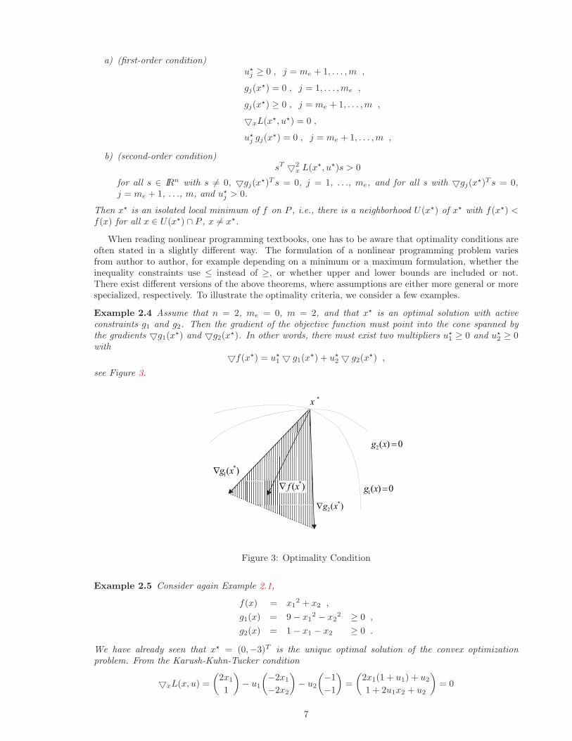
Example 2.4 Assume that n = 2, me = 0, m = 2, and that x� is an optimal solution with activeconstraints g1 and g2. Then the gradient of the objective function must point into the cone spanned bythe gradients �g1(x�) and �g2(x�). In other words, there must exist two multipliers u�

1 ≥ 0 and u�2 ≥ 0

with�f(x�) = u�

1 � g1(x�) + u�2 � g2(x�) ,

see Figure 3.

Figure 3: Optimality Condition

Example 2.5 Consider again Example 2.1,

f(x) = x12 + x2 ,

g1(x) = 9 − x12 − x2

2 ≥ 0 ,

g2(x) = 1 − x1 − x2 ≥ 0 .

We have already seen that x� = (0,−3)T is the unique optimal solution of the convex optimizationproblem. From the Karush-Kuhn-Tucker condition

�xL(x, u) =(

2x1

1

)− u1

(−2x1

−2x2

)− u2

(−1−1

)=(

2x1(1 + u1) + u2

1 + 2u1x2 + u2

)= 0

7

we get the multipliers u�1 = 1/6 und u�

2 = 0. Moreover, the Hessian matrix of the Lagrangian function

�2xL(x�, u�) =

(7/3 00 1/3

)

is positive definite.

3 The Quadratic Programming Subproblem and the AugmentedLagrangian Merit Function

Sequential quadratic programming or SQP methods belong to the most powerful nonlinear programmingalgorithms we know today for solving differentiable nonlinear programming problems of the form (2).The theoretical background is described e.g. in Stoer [58] in form of a review, or in Spellucci [57] in formof an extensive text book. From the more practical point of view, SQP methods are also introduced in thebooks of Papalambros, Wilde [33] and Edgar, Himmelblau [14]. Their excellent numerical performancewas tested and compared with other methods in Schittkowski [39], and since many years they belong tothe most frequently used algorithms to solve practical optimization problems.

The basic idea is to formulate and solve a quadratic programming subproblem in each iterationwhich is obtained by linearizing the constraints and approximating the Lagrangian function L(x, u) (5)quadratically, where x ∈ IRn is the primal and u = (u1, . . . , um)T ∈ IRm the dual variable, i.e., themultiplier vector. Assume that xk ∈ IRn is an actual approximation of the solution, vk ∈ IRm anapproximation of the multipliers, and Bk ∈ IRn×n an approximation of the Hessian of the Lagrangianfunction all identified by an iteration index k. Then a quadratic programming subproblem of the form

minimize 12dT Bkd + ∇f(xk)T d

d ∈ IRn : ∇gj(xk)T d + gj(xk) = 0 , j ∈ E,

∇gj(xk)T d + gj(xk) ≥ 0 , j ∈ I

(8)

is formulated and must be solved in each iteration. Here we introduce index sets E.= {1, . . . , me} and

I.= {me +1, . . . ,m}. Let dk be the optimal solution, uk the corresponding multiplier of this subproblem,

and denote by

zk.=(

xk

vk

), pk

.=(

dk

uk − vk

)(9)

the composed iterate zk and search direction xk. A new iterate is obtained by

zk+1.= zk + αkpk , (10)

where αk ∈ (0, 1] is a suitable steplength parameter.To motivate the formulation of the particular subproblem, let me = m for simplicity, i.e., we assume

for a moment that there are no inequality constraints. The Karush-Kuhn-Tucker optimality conditions(6) are then written in the form (�xL(x, v)

g(x)

)= 0

with g(x) = (g1(x), . . . , gm(x))T . In other words, the optimal solution and the corresponding multipliersare the solution of a system of n + m nonlinear equations F (z) = 0 with n + m unknowns z = (x, v),where

F (z) =( �xL(x, v)

g(x)

).

Let zk = (xk, vk) be an approximation of the solution. We apply Newton’s method and get an estimatefor the next iterate by

�F (zk)qk + F (zk) = 0 .

After insertion, we obtain the equation(Bk : −� g(xk)

�g(xk)T : 0

)(dk

yk

)+(�f(xk) −�g(xk)vk

g(xk)

)= 0

8

with Bk = �2xL(xk, vk), where qk = (dk, yk). Defining now uk = yk + vk, we get

Bkdk −�g(xk)uk + �f(xk) = 0

and�g(xk)T dk + g(xk) = 0 .

But these equations are exactly the optimality conditions for the quadratic programming subproblem.To sum up, we come to the following conclusion:

A sequential quadratic programming method is identical to Newton’s method of solvingthe necessary optimality conditions, if Bk is the Hessian of the Lagrangian function and ifwe start sufficiently close to a solution.

Now we assume that inequality constraints are again permitted, i.e., me ≤ m. A straightforwardanalysis shows that if dk = 0 is an optimal solution of (8) and uk the corresponding multiplier vector,then xk and uk satisfy the necessary optimality conditions of (2).

However, the linear constraints in (8) can become inconsistent even if we assume that the originalproblem (2) is solvable. As in Powell [34], we add an additional variable δ to (8) and solve an (n + 1)-dimensional subproblem with consistent constraints.

Another numerical drawback of (8) is that gradients of all constraints must be reevaluated in eachiteration step. But if xk is close to the solution, the calculation of the gradients of inactive nonlinearconstraints is redundant. Given a constant ε > 0, we define the sets

I(k)

1 = {j ∈ I : gj(xk) ≤ ε or v(k)j > 0}, I

(k)

2 = I \ I(k)

1 (11)

and solve the following subproblem at each step,

minimize 12dT Bkd + ∇f(xk)T d + 1

2�kδ2

d ∈ IRn, δ ∈ [0, 1] : ∇gj(xk)T d + (1 − δ)gj(xk) = 0, j ∈ E,

∇gj(xk)T d + (1 − δ)gj(xk) ≥ 0, j ∈ I(k)

1 ,

∇gj(xk(j))T d + gj(xk) ≥ 0, j ∈ I(k)

2 .

(12)

The indices k(j) ≤ k denote previous iterates where the corresponding gradient has been evaluated thelast time. We start with I

(0)

1.= I and I

(0)

2.= ∅ and reevaluate constraint gradients in subsequent iterations

only if the constraint belongs to the active set I(k)

1 . The remaining rows of the Jacobian matrix remainfilled with previously computed gradients.

We denote by (dk, uk) the solution of (12), where uk is the multiplier vector, and by δk the additionalvariable to prevent inconsistent linear constraints. Under a standard regularity assumption, i.e., theconstraint qualification, it is easy to see that δk < 1.

Bk is a positive-definite approximation of the Hessian of the Lagrange function. For the globalconvergence analysis presented in this paper, any choice of Bk is appropriate as long as the eigenvaluesare bounded away from zero. However, to guarantee a superlinear convergence rate, we update Bk bythe BFGS quasi-Newton method

Bk+1.= Bk +

akaTk

bTk ak

− BkbkbTk Bk

bTk Bkbk

(13)

withak

.= �xL(xk+1, uk) −�xL(xk, uk),bk

.= xk+1 − xk.(14)

Usually, we start with the unit matrix for B0 and stabilize the formula by requiring that aTk bk ≥

0.2 bTk Bkbk, see Powell [34], Stoer [58], or Schittkowski [41]. A penalty parameter �k is required to

reduce the perturbation of the search direction by the additional variable δ as much as possible, seeSchittkowski [43] for a motivation and a formula.

To enforce global convergence of the SQP method, we have to select a suitable penalty parameter rk

and to select a steplength αk, see (10), subject to a merit function φk(α). To avoid the Maratos effect,

9

a certain irregularity leading to infinite cycles, we use the differentiable augmented Lagrange function ofRockafellar [38],

Φr(x, v) .= f(x) −∑

j∈E∪I1

(vjgj(x) − 12rjgj(x)2) − 1

2

∑j∈I2

v2j /rj , (15)

with r = (r1, . . . , rm)T , I1.= {j ∈ I : gj(x) ≤ vj/rj} and I2

.= I \I1, cf. Schittkowski [43]. The meritfunction is then defined by

φk(α) .= Φrk+1(zk + αpk), (16)

see also (9). To ensure that pk is a descent direction of Φrk+1(zk), i.e., that

φ′k(0) = ∇Φrk+1(zk)T pk < 0 , (17)

the new penalty parameter rk+1 must be selected carefully. Each coefficient r(k)j of rk is updated by

r(k+1)j

.= max

(σ

(k)j r

(k)j ,

2m(u(k)j − v

(k)j )

(1 − δk)dTk Bkdk

)(18)

for j = 1, . . . ,m. The sequence {σ(k)j } is introduced to allow decreasing penalty parameters at least in the

beginning of the algorithm by assuming that σ(k)j ≤ 1. A a sufficient condition to guarantee convergence

of {r(k)j } is that there exists a positive constant ζ with

∞∑k=0

[1 − (σ(k)

j )ζ]

< ∞ . (19)

for j = 1, . . . ,m.

Example 3.1 Consider Example 2.1, where the optimization problem is given by

min x12 + x2

x1, x2 : 9 − x12 − x2

2 ≥ 0 ,

1 − x1 − x2 ≥ 0 .

Proceeding from the starting values x0 = (2, 0)T and the identity matrix for B0, we get the quadraticprogramming subproblem

min 12d1

2 + 12d2

2 + 4d1 + d2

d1, d2 : −4d1 + 5 ≥ 0 ,

−d1 − d2 − 1 ≥ 0 .

Since none of the linear constraints is active at the unconstrained minimum, the solution is d0 =(−4,−1)T with multiplier vector u0 = (0, 0)T . Assuming that α0 = 1, x1 = (−2,−1)T is the next iterate.The new approximation of the Hessian of the Lagrangian function, B1, is computed by one update of theBFGS method

B1 = B0 +a0a

T0

bT0 a0

− B0b0bT0 B0

bT0 B0b0

,

a0 = �xL(x1, u0) −�xL(x0, u0) = �f(x1) −�f(x0) =(−8

0

),

b0 = x1 − x0 =(−4−1

).

Then

B1 =(

1 00 1

)+

132

(64 00 0

)− 1

17

(16 44 1

)≈(

2 − 14

− 14 1

).

10

The new quadratic programming subproblem is

min d12 + 1

2d22 − 1

4d1d2 − 4d1 + d2

d1, d2 : 4d1 + 2d2 + 4 ≥ 0 ,

−d1 − d2 + 4 ≥ 0 .

Again, the unconstrained solution is feasible and

d1 =131

(60

−16

), u1 =

(00

)

is the optimal solution of the subproblem. Assuming that the steplength is 1, the new iterate is

x2 =131

( −2−47

).

4 An SQP Algorithm with Non-monotone Line Search and Dis-tributed Function Evaluations

The implementation of a line search algorithm is a critical issue when implementing a nonlinear program-ming algorithm, and has significant effect on the overall efficiency of the resulting code. On the one handwe need a line search to stabilize the algorithm, on the other hand it is not advisable to waste too manyfunction calls. Moreover, the behavior of the merit function becomes irregular in case of constrained op-timization because of very steep slopes at the border caused by penalty terms. Even the implementationis more complex than shown below, if linear constraints or bounds for variables are to be satisfied duringthe line search.

Typically, the steplength αk is chosen to satisfy the Armijo [1] condition

φk(αk) ≤ φk(0) + µαkφ′k(0) , (20)

see for example Ortega and Rheinboldt [31], or any other related stopping rule. Since pk is a descentdirection, i.e., φ′

k(0) < 0, we achieve at least a sufficient decrease of the merit function at the next iterate.The test parameter µ must be positive and not greater than 0.5.

The parameter αk is chosen by a separate algorithm which should take the curvature of the meritfunction into account. If αk is too small, the line search terminates very fast, but the resulting stepsizesmight become too small leading to a higher number of outer iterations. On the other hand, a largervalue close to one requires too many function calls during the line search. Thus, we need some kind ofcompromise which is obtained by applying first a polynomial interpolation, typically a quadratic one,combined with a bisection strategy in irregular situations, if the interpolation scheme does not lead to areasonable new guess. (20) is then used as a stopping criterion.

However, practical experience shows that monotonicity requirement of (20) is often too restrictiveespecially in case of very small values of φ′

r(0), which are caused by numerical instabilities during thesolution of the quadratic programming subproblem or, more frequently, by inaccurate gradients. Toavoid interruption of the whole iteration process, the idea is to conduct a line search with a more relaxedstopping criterion. Instead of testing (20), we accept a stepsize αk as soon as the inequality

φk(αk) ≤ maxk−l(k)≤j≤k

φj(0) + µαkφ′k(0) (21)

is satisfied, where l(k) is a predetermined parameter with l(k) ∈ {0, . . . ,min(k, L)}, L a given tolerance.Thus, we allow an increase of the reference value φrjk

(0), i.e. an increase of the merit function value. ForL = 0, we get back the original criterion (20).

To implement the non-monotone line search, we need a queue consisting of merit function values atprevious iterates. We allow a variable queue length l(k) which can be adapted by the algorithm, forexample, if we want to apply a standard monotone line search as long as it terminates successfully withina given number of steps and to switch to the non-monotone one otherwise.

The idea to store reference function values and to replace the sufficient descent property by a suffi-cient ’ascent’ property, is for example described in Dai [11], where a general convergence proof for the

11

unconstrained case is presented. The general idea goes back to Grippo, Lampariello, and Lucidi [17],and was extended to constrained optimization and trust region methods in a series of subsequent pa-pers, see Bonnans et al. [4], Grippo et al. [18, 19], Ke et al. [28], Panier and Tits [32], Raydan [37], andToint [60, 61].

To summarize, we obtain the following non-monotone line search algorithm based on quadratic in-terpolation and an Armijo-type bisection rule which can be applied in the k-th iteration step of an SQPalgorithm:

Algorithm 4.1 Let β, µ with 0 < β < 1 and 0 < µ < 0.5 be given, further an integer l(k) ≥ 0.

Start: αk,0.= 1

For i = 0, 1, 2, . . . do:1) If φk(αk,i) < maxk−l(k)≤j≤k φj(0) + µ αk,i φ′

k(0), let ik.= i, αk

.= αk,ikand

stop.

2) Compute αk,i.=

0.5 α2k,i φ′

r(0)αk,iφ′

r(0) − φr(αk,i) + φr(0).

3) Let αk,i+1.= max(β αk,i, αk,i).

Corresponding convergence results for the monotone case, i.e., L = 0, are found in Schittkowski [43].αk,i is the minimizer of the quadratic interpolation and we use a relaxed Armijo-type descent propertyfor checking termination. Step 3) is required to avoid irregular situations. For example, the minimizer ofthe quadratic interpolation could be outside of the feasible domain (0, 1]. The line search algorithm mustbe implemented together with additional safeguards, for example to prevent violation of bounds and tolimit the number of iterations.

The increasing numerical complexity of practical optimization problems requires a careful redesignof SQP methods to allow simultaneous function evaluations. On the one hand, distributed functioncalls can be used to approximate derivatives by difference formulae without influencing the nonlinearprogramming algorithm at all. However, the line search algorithm requires the serial computation ofφk(αk,i), i = 1, 2, . . .. Thus, Algorithm 4.1 is further modified to allow parallel function calls.

To outline the approach, let us assume that functions can be computed simultaneously on P differentmachines, P ≥ 1. Then P test values αk,i

.= βi−1 with β = ε1/(P−1) are selected, i = 1, . . ., P , where εis a guess for the machine precision. We require P parallel function calls to get the corresponding modelfunction values. The largest αk,i satisfying a sufficient descent property (21), say for i = ik, is acceptedas the new steplength for getting the subsequent iterate with αk

.= αk,ik. For an alternative approach

based on pattern search, see Hough, Kolda, and Torczon [26].The proposed parallel line search will work efficiently, if the number of parallel machines P is suffi-

ciently large, and is summarized as follows:

Algorithm 4.2 Let β, µ with 0 < β < 1 and 0 < µ < 0.5 be given, further two integers P ≥ 1 andl(k) ≥ 0.

Start: For αk,i.= βi compute φk(αk,i) for i = 0, . . ., P − 1.

For i = 0, 1, 2, . . . do:If φk(αk,i) < maxk−l(k)≤j≤k φj(0) + µ αk,i φ′

k(0), let ik.= i, αk

.= αk,ikand

stop.

To precalculate P candidates at log-distributed points between a small tolerance α = τ and α = 1,0 < τ << 1, we propose β = τ1/(P−1).

The paradigm of parallelism is SPMD, i.e., Single Program Multiple Data. In a typical situation wesuppose that there is a complex application code providing simulation data, for example by an expensiveFinite Element calculation in mechanical structural optimization. It is supposed that various instances ofthe simulation code providing function values are executable on a series of different machines controlledby a master program that executes an optimization algorithm. By a message passing system, for examplePVM, see Geist et al. [15], only very few data need to be transferred from the master to the slaves.Typically only a set of design parameters of length n must to be passed. On return, the master acceptsnew model responses for objective function and constraints, at most m+1 double precision numbers. All

12

massive numerical calculations and model data, for example to compute the stiffness matrix of a FiniteElement model in a mechanical engineering application, remain on the slave processors of the distributedsystem.

Now we are able to formulate the SQP algorithm for solving the constrained nonlinear programmingproblem (2), see Schittkowski [40, 41, 43] for further details. First, we have to select a couple of realconstants ε, β, µ, δ, �, ε and of integer constants L and P , that are not changed within the algorithmand that satisfy

ε ≥ 0 , 0 ≤ β ≤ 1 , 0 ≤ δ < 1 , � > 1 , ε > 0, , L ≥ 0 , P ≥ 1.

Choose starting values x0 ∈ IRn, v0 ∈ IRm with v(0)j ≥ 0 for j ∈ I, B0 ∈ IRn×n positive definite, � ∈ IR

with � > 0, and r0 ∈ IRm with r(0)j > 0 for j = 1, . . ., m. Moreover, we set I

(0)

1.= I and I

(0)

2.= ∅.

The main steps consist of the following instructions:

Algorithm 4.3 Start: Evaluate f(x0), ∇f(x0), gj(x0), and ∇gj(x0), j = 1, ..., m.For k = 0, 1, 2, ... compute xk+1, vk+1, Bk+1, rk+1, �k+1, and I

(k+1)1 as follows:

Step 1. Solve the quadratic programming subproblem (12) and denote by dk, δk the optimal solution andby uk the optimal multiplier vector. If δk ≥ δ, let �k

.= ��k and solve (12) again

Step 2. Determine a new penalty parameter rk+1 by (18).

Step 3. If φ′k(0) ≥ 0, let �k

.= ��k and go to Step 1.

Step 4. Define the new penalty parameter �k+1.

Step 5. Choose a queue length l(k), 0 ≤ l(k) ≤ L, to apply Algorithm 4.1 in case of P = 1 or Algo-rithm 4.2 otherwise with respect to the merit function φk(α), see (16), to get a steplength αk.

Step 6. Let xk+1.= xk +αkdk, vk+1

.= vk +αk(uk − vk) be new iterates and evaluate f(xk+1), gj(xk+1),

j = 1, . . ., m, ∇f(xk+1), I(k+1)

1 by (11), and ∇gj(xk+1), j ∈ E ∪ I(k+1)

1 .

Step 7. Compute a suitable new positive-definite approximation of the Hessian of the Lagrange functionBk+1 by (13), set k

.= k + 1, and repeat the iteration.

To implement Algorithm 4.3, various modifications are necessary. Despite of a theoretically well-defined procedure, the practical code might fail because of round-off errors or violations of some assump-tions. For example, we need additional bounds to limit the number of cycles in Step 1, between Step 3and Step 1, in the line search, and to limit the number of outer iteration steps. The tolerance ε whichis used to determine active constraints by (11), serves also as a stopping criterion. The implementationNLPQL of Schittkowski [44, 54] applies several criteria, either simultaneously or in an alternative way,e.g.,

dTk Bkdk < ε2 ,

| � f(xk)T dk| +∑m

j=1 |u(k)j gj(xk)| < ε ,

‖ �x L(xk, uk)‖ <√

ε ,∑mj=1 |gj(xk)| +∑m

j=me+1 |min(0, gj(xk))| <√

ε .

(22)

There remain a few comments to illustrate some further algorithmic details. Most of them are basedon empirical investigations or some experience obtained from a large number of practical applications.

1. Although it is sometimes possible to find a reasonable good starting point x0, it is often impossibleto get an initial guess for the Hessian the Lagrange function and the multipliers. Thus, the choiceof B0

.= I, where I denotes the n by n identity matrix, and v.= 0 is often used in practice.

2. The BFGS formula (13) can be replaced by an equivalent formula for the factors of a Choleskydecomposition Bk = LkLT

k , where Lk is a lower triangular matrix.

13

3. The quadratic programming subproblem can be solved by any available black-box algorithm. Ifa Cholesky decomposition is updated as outlined before, the choice of a primal-dual algorithmis recommended, see e.g. Powell [36]. The additional variable ρ requires the introduction of anadditional column and row to Bk, where the lowest diagonal element contains the penalty parameterρk.

4. Since the introduction of the additional variable δ leads to an undesired perturbation of the searchdirection, it is recommended to solve first problem (8) without the additional variable and tointroduce ρ only in case of a non-successful return.

5. It is recommended to start the line search procedure with l(k) .= 0 and to switch to the non-monotone case l(k) .= L only if αk cannot be computed within a given number of steps.

6. The parallel line search with a limited number of available merit function values seems to berestrictive and seems to require additional theoretical convergence assumptions, since the analysisof the subsequent section is not able to predetermine the required number of cycles or sub-iterations,see also the above comments. However, a practical implementation of the non-monotone line searchprocedure of Algorithm 4.1 also needs a fixed limitation of the number of iterations. Thus, weassume for simplicity that P is sufficiently big.

Example 4.1 Consider Example 2.1 again, where the optimization problem is given by

min x12 + x2

x1, x2 : 9 − x12 − x2

2 ≥ 0 ,

1 − x1 − x2 ≥ 0 .

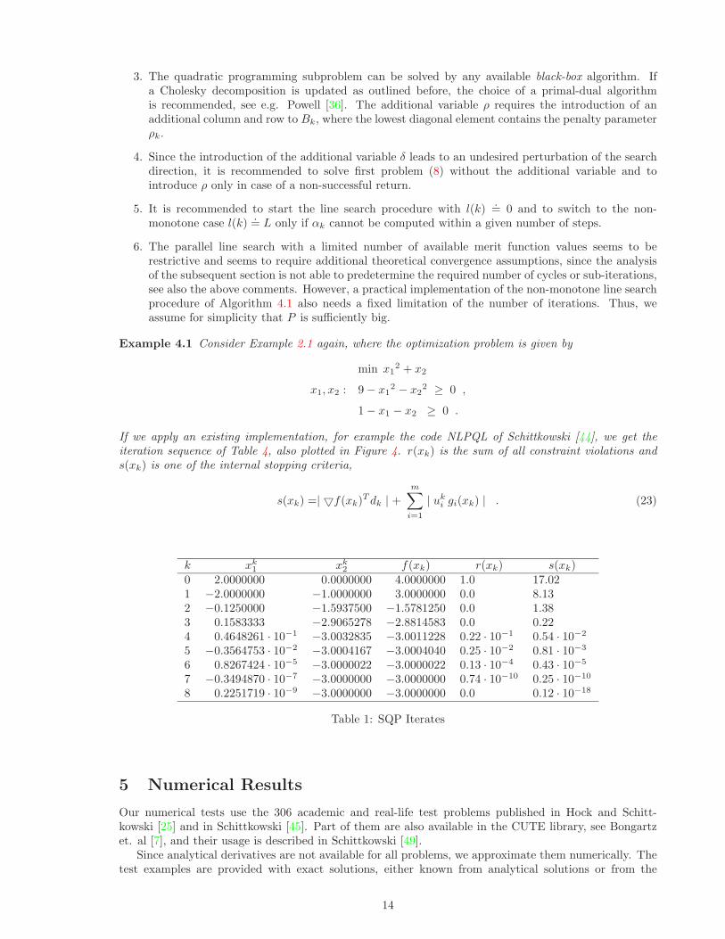
If we apply an existing implementation, for example the code NLPQL of Schittkowski [44], we get theiteration sequence of Table 4, also plotted in Figure 4. r(xk) is the sum of all constraint violations ands(xk) is one of the internal stopping criteria,

s(xk) =| �f(xk)T dk | +m∑

i=1

| uki gi(xk) | . (23)

k xk1 xk

2 f(xk) r(xk) s(xk)0 2.0000000 0.0000000 4.0000000 1.0 17.021 −2.0000000 −1.0000000 3.0000000 0.0 8.132 −0.1250000 −1.5937500 −1.5781250 0.0 1.383 0.1583333 −2.9065278 −2.8814583 0.0 0.224 0.4648261 · 10−1 −3.0032835 −3.0011228 0.22 · 10−1 0.54 · 10−2

5 −0.3564753 · 10−2 −3.0004167 −3.0004040 0.25 · 10−2 0.81 · 10−3

6 0.8267424 · 10−5 −3.0000022 −3.0000022 0.13 · 10−4 0.43 · 10−5

7 −0.3494870 · 10−7 −3.0000000 −3.0000000 0.74 · 10−10 0.25 · 10−10

8 0.2251719 · 10−9 −3.0000000 −3.0000000 0.0 0.12 · 10−18

Table 1: SQP Iterates

5 Numerical Results

Our numerical tests use the 306 academic and real-life test problems published in Hock and Schitt-kowski [25] and in Schittkowski [45]. Part of them are also available in the CUTE library, see Bongartzet. al [7], and their usage is described in Schittkowski [49].

Since analytical derivatives are not available for all problems, we approximate them numerically. Thetest examples are provided with exact solutions, either known from analytical solutions or from the

14

-4

-3

-2

-1

0

1

2

3

4

-6 -5 -4 -3 -2 -1 0 1 2 3 4 5 6

g2(x) = 0f(x) = c

g1(x) = 0

x1

x2

�

�

��

���

�

�

���

Figure 4: SQP Iterates

best numerical data found so far. The Fortran codes are compiled by the Intel Visual Fortran Compiler,Version 8.0, under Windows XP, and executed on a Pentium IV processor with 2.8 GHz. Total calculationtime for solving the test problems with forward differences for the gradient approximation is about 1 sec.

First we need a criterion to decide, whether the result of a test run is considered as a successfulreturn or not. Let ε > 0 be a tolerance for defining the relative accuracy, xk the final iterate of a testrun, and x� the supposed exact solution known from the two test problem collections. Then we call theoutput a successful return, if the relative error in the objective function is less than ε and if the maximumconstraint violation is less than ε2, i.e. if

f(xk) − f(x�) < ε|f(x�)| , if f(x�) <> 0

orf(xk) < ε , if f(x�) = 0

andr(xk) .= max(‖g(xk)+‖∞) < ε2 ,

where ‖ . . . ‖∞ denotes the maximum norm and gj(xk)+ .= −min(0, gj(xk)) for j > me and gj(xk)+ .=gj(xk) otherwise.

We take into account that a code returns a solution with a better function value than the knownone within the error tolerance of the allowed constraint violation. However, there is still the possibilitythat an algorithm terminates at a local solution different from the given one. Thus, we call a testrun a successful one, if the internal termination conditions are satisfied subject to a reasonably smalltermination tolerance, and if in addition to the above decision,

f(xk) − f(x�) ≥ ε|f(x�)| , if f(x�) <> 0

orf(xk) ≥ ε , if f(x�) = 0

andr(xk) < ε2 .

For our numerical tests, we use ε = 0.01, i.e., we require a final accuracy of one per cent. Gradientsare approximated by the forward difference formula:

∂

∂xif(x) ≈ 1

ηi

(f(x + ηiei) − f(x)

)(24)

Here ηi = η max(10−5, |xi|) and ei is the i-th unit vector, i = 1, . . . , n. The tolerance η depends on thedifference formula and is set to η = ηm

1/2, where ηm is a guess for the accuracy by which function values

15

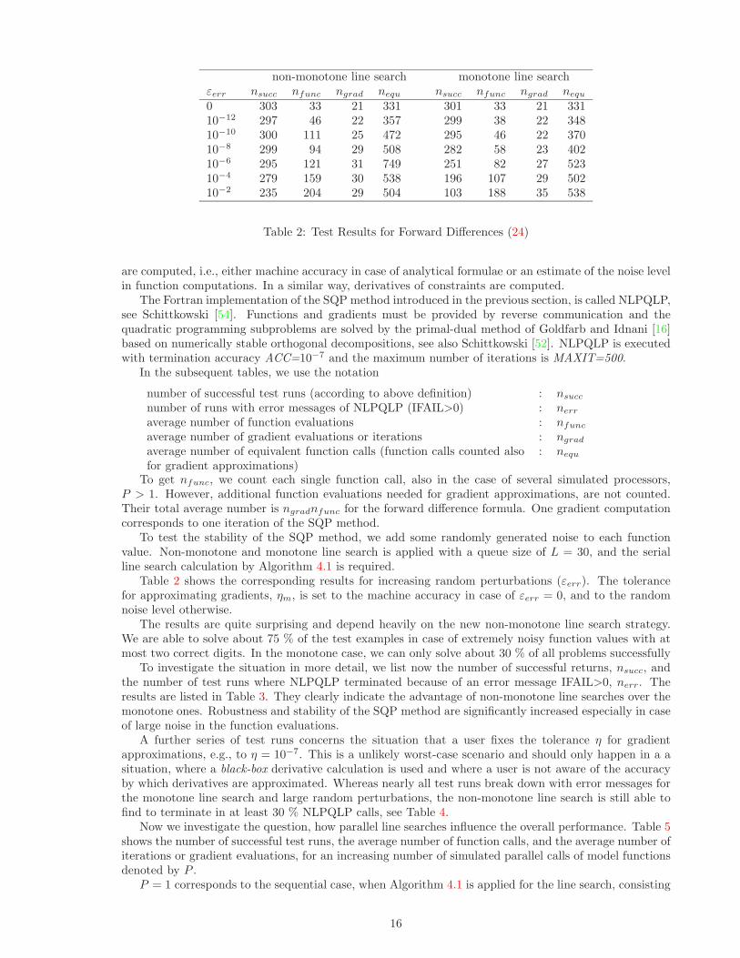
non-monotone line search monotone line searchεerr nsucc nfunc ngrad nequ nsucc nfunc ngrad nequ

0 303 33 21 331 301 33 21 33110−12 297 46 22 357 299 38 22 34810−10 300 111 25 472 295 46 22 37010−8 299 94 29 508 282 58 23 40210−6 295 121 31 749 251 82 27 52310−4 279 159 30 538 196 107 29 50210−2 235 204 29 504 103 188 35 538

Table 2: Test Results for Forward Differences (24)

are computed, i.e., either machine accuracy in case of analytical formulae or an estimate of the noise levelin function computations. In a similar way, derivatives of constraints are computed.

The Fortran implementation of the SQP method introduced in the previous section, is called NLPQLP,see Schittkowski [54]. Functions and gradients must be provided by reverse communication and thequadratic programming subproblems are solved by the primal-dual method of Goldfarb and Idnani [16]based on numerically stable orthogonal decompositions, see also Schittkowski [52]. NLPQLP is executedwith termination accuracy ACC=10−7 and the maximum number of iterations is MAXIT=500.

In the subsequent tables, we use the notation

number of successful test runs (according to above definition) : nsucc

number of runs with error messages of NLPQLP (IFAIL>0) : nerr

average number of function evaluations : nfunc

average number of gradient evaluations or iterations : ngrad

average number of equivalent function calls (function calls counted alsofor gradient approximations)

: nequ

To get nfunc, we count each single function call, also in the case of several simulated processors,P > 1. However, additional function evaluations needed for gradient approximations, are not counted.Their total average number is ngradnfunc for the forward difference formula. One gradient computationcorresponds to one iteration of the SQP method.

To test the stability of the SQP method, we add some randomly generated noise to each functionvalue. Non-monotone and monotone line search is applied with a queue size of L = 30, and the serialline search calculation by Algorithm 4.1 is required.

Table 2 shows the corresponding results for increasing random perturbations (εerr). The tolerancefor approximating gradients, ηm, is set to the machine accuracy in case of εerr = 0, and to the randomnoise level otherwise.

The results are quite surprising and depend heavily on the new non-monotone line search strategy.We are able to solve about 75 % of the test examples in case of extremely noisy function values with atmost two correct digits. In the monotone case, we can only solve about 30 % of all problems successfully

To investigate the situation in more detail, we list now the number of successful returns, nsucc, andthe number of test runs where NLPQLP terminated because of an error message IFAIL>0, nerr. Theresults are listed in Table 3. They clearly indicate the advantage of non-monotone line searches over themonotone ones. Robustness and stability of the SQP method are significantly increased especially in caseof large noise in the function evaluations.

A further series of test runs concerns the situation that a user fixes the tolerance η for gradientapproximations, e.g., to η = 10−7. This is a unlikely worst-case scenario and should only happen in a asituation, where a black-box derivative calculation is used and where a user is not aware of the accuracyby which derivatives are approximated. Whereas nearly all test runs break down with error messages forthe monotone line search and large random perturbations, the non-monotone line search is still able tofind to terminate in at least 30 % NLPQLP calls, see Table 4.

Now we investigate the question, how parallel line searches influence the overall performance. Table 5shows the number of successful test runs, the average number of function calls, and the average number ofiterations or gradient evaluations, for an increasing number of simulated parallel calls of model functionsdenoted by P .

P = 1 corresponds to the sequential case, when Algorithm 4.1 is applied for the line search, consisting

16

non-monotone monotoneεerr nsucc nerr nsucc nerr

0 303 3 301 1010−12 297 8 299 2710−10 300 8 295 5810−8 299 8 282 10610−6 295 24 251 15910−4 279 44 196 21010−2 235 78 103 251

Table 3: Successful and Non-Successful Returns

non-monotone monotoneεerr nsucc nerr nsucc nerr

0 303 4 301 1210−12 300 4 299 3510−10 295 14 278 8310−8 265 43 196 14510−6 183 124 49 26510−4 114 194 13 29810−2 108 199 23 288

Table 4: Successful and Non-Successful Returns, η = 10−7

P nsucc nfunc ngrad

1 303 33 213 237 434 1364 265 442 1085 291 318 636 296 235 387 298 220 318 296 223 279 299 231 25

10 296 241 2415 299 342 2320 298 466 2350 299 1,146 23

Table 5: Performance Results for Parallel Line Search

17

of a quadratic interpolation combined with an Armijo-type bisection strategy. Since we need at least onefunction evaluation for the subsequent iterate, we observe that the average number of additional functionevaluations needed for the line search, is about two.

In all other cases, P > 1 simultaneous function evaluations are made according to Algorithm 4.2.Thus, the total number of function calls nfunc is quite big in Table 5. If, however, the number ofparallel machines is sufficiently large in a practical situation, we need only one simultaneous functionevaluation in each step of the SQP algorithm. To get a reliable and robust line search, we need at least 5parallel processors. No significant improvements are observed, if we have more than 10 parallel functionevaluations.

The most promising possibility to exploit a parallel system architecture occurs, when gradients cannotbe calculated analytically, but have to be approximated numerically, for example by forward differences,two-sided differences, or even higher order methods. Then we need at least n additional function calls,where n is the number of optimization variables, or a suitable multiple of n.

6 Numerical Pitfalls

A particular advantage od SQP methods is their numerical stability and robustness. Only very fewparameters must be set to call the corresponding code, typically only the maximum number of iterationsand a termination tolerance. Nevertheless numerous pitfalls and traps exist which can occur during themodelling process and which can prevent a successful and efficient solution. We show some remedies andoutline how to avoid them that at least in certain situations.

6.1 Inappropriate Termination Accuracy

Termination of an SQP algorithm depends on certain conditions, in our case summarized by some checks(22), and a tolerance ε > 0. The choice of ε is crucial for the overall success of an optimization run. A toosmall value could prevent successful termination completely, since internal round-off errors can preventsatisfaction of (22). On the other hand, a too big value stops the algorithm at an intermediate iterateand we do not know by sure, whether at least a local solution is approximated or not.

On the other hand, the calculation of a search direction mainly depends on the accuracy by whichgradients are computed. Objective function values, for example, are not part of the quadratic program-ming subproblem (8) at all. Only the line search requires function values, but the strategy is to reachthe stopping criterion (20) as early as possible.

Thus, a reasonable recommendation is to choose an ε > 0 which is in the order or even a bit higherthan the accuracy by which gradients are computed.

6.2 Violation of Constraint Qualification

A certain regularity condition called constraint qualification is required for being able to formulate thenecessary optimality conditions, see Definition 2.3. However, also the local convergence theorems andmost solvers for the underlying quadric program depend on the validity of this assumption at least inthe neighborhood of an optimal solution. In general, it is not possible to validate this condition a priorybefore starting an optimization algorithm. On the other hand, the evaluation of active constraints andthe rank determination of the Jacobian of the active constraints depends on a predetermined tolerance,which is be difficult to setup a priory.

If an optimization problem (2) does not satisfy this assumption when approaching a local minimum,the corresponding code typically slows down convergence speed and superlinear convergence is prevented.In other cases, the SQP algorithm could stop because of numerical instabilities when trying to solve thequadratic programming problem (8).

At least in some simple situations, it is possible to prevent violation of the constraint qualification.Consider, for example, a problem with an equality constraint g(x) = 0, but the available implementationis unable to handle equality constraints directly as is the case for many structural design optimizationcodes. The straightforward transformation of each equality constraint to two inequality constraints ofthe form g(x) ≥ 0 and −g(x) ≥ 0, however, should be prevented. In this case, the constraint qualificationis always violated.

18

6.3 Non-Differentiable Model Functions

In most practical and complex applications, it not guaranteed that the model functions by which f(x)and gj(x), j = 1, . . ., are computed, are continuously differentiable as required. A typical simple standardsituation is found if the nonlinear program consists of minimizing the maximum or the sum of absolutevalues of differentiable functions f1(x), . . ., fp(x),

x ∈ IRn :

min max{fi(x) : i = 1, . . . , p}gj(x) = 0 , j = 1, . . . ,me ,

gj(x) ≥ 0 , j = me + 1, . . . , m ,

(25)

or

x ∈ IRn :

min∑p

i=1 |fi(x)|gj(x) = 0 , j = 1, . . . ,me ,

gj(x) ≥ 0 , j = me + 1, . . . , m .

(26)

In the first case, we add one additional variable and p additional constraints, and get

x ∈ IRn+1 :

min xn+1

gj(x) = 0 , j = 1, . . . , me ,

gj(x) ≥ 0 , j = me + 1, . . . ,m ,

fi(x) ≤ xn+1 , i = 1, . . . , p ,

(27)

in the second case, we add p additional variables and 2p additional constraints,

x ∈ IRn+p :

min∑p

i=1 xn+i

gj(x) = 0 , j = 1, . . . ,me ,

gj(x) ≥ 0 , j = me + 1, . . . , m ,

fi(x) ≤ xn+i , i = 1, . . . , p ,

fi(x) ≥ −xn+i , i = 1, . . . , p .

(28)

We obtain equivalent nonlinear programs of the form (2) which can be solved by any algorithm for smoothoptimization.

However, the general situation is much more complex and cannot be resolved in the same simpleway. Sometimes, a careful gradient calculation based on smooth approximations are applicable. In thesimulation code by which objective function and constraint function values are computed, one could tryto prevent typical situations leading to instabilities by hand, e.g., by smoothing techniques. For example,the Kreiselmeier-Steinhauser function is often used to smoothen the maximum function by

Ψ(x) =1ρ

log

(p∑

i=1

exp(ρfi(x)

).

6.4 Empty Feasible Domains

There is no mathematical criterion nor any applicable numerical method that allows us to detect whetherthe feasible domain P of (2) is empty or not. Infeasible domains occur for example in case of modellingerrors or programming bugs, but also in a systematical way. The subsequent case study of Section 8, thedesign of surface acoustic wave filters, is a typical example. If the design demands of a customer are toostringent, the feasible domain of (37) is empty.

A simple remedy is to perform a certain regularization of (1) by introducing an additional variablexn+1 of the form

x ∈ IRn+1 :

min f(x) + ρxn+1

gj(x) ≥ −xn+1 , j = me + 1, . . . , m ,

xl ≤ x ≤ xu , xn+1 ≥ 0 .

(29)

For simplicity, we omit the equality constraints. A penalty parameter ρ is to reduce the additionalperturbation of the solution by xn+1 as much as possible, and must be chosen carefully.

19

6.5 Undefined Model Function Values

SQP methods have a particular practical advantage. Linear constraints and bounds of variables remainsatisfied in all iterations, if the starting point x0 satisfies them. Thus, these constraints can be used toprevent undefined function calls. For example, if the simulation code for computing f(x) or any of theconstraints gj(x), j = 1, . . ., m, contains an expression of the form log(aT x), it is recommended to adda constraint of the form gm+1(x) .= aT x − ε, ε > 0.

In general, however, it is not possible to prevent a function call from the infeasible domain. If thereis an internal error code, one could try to return a function value of the form δ‖xk − x‖ with x ∈ P . Butif the corresponding constraint becomes active at a solution, we will run into an instability and an SQPcode will break done with an error message. In such a situation, it is recommended to shrink the feasibleset by replacing gj(x) by gj(x) − δ, δ > 0, and to adapt δ step-by-step.

6.6 Wrong Function and Variable Scaling

There is no way to find a general scaling routine which automatically predetermines perfect scalingparameters for optimization variables and constraints. The goal is to find positive numbers by which allfunctions and all individual variables are multiplied, so that, roughly speaking, a change of the scaledvariables in the order of one leads to an alteration of the scaled function values in the order of one.However, these coefficients can be determined only at the very beginning of an optimization run basedon some information available at the starting point x0.

But depending on the application, it is sometimes possible to scale the problem in a suitable way.If some constraints have a physical background to prevent them from exceeding an upper bound, forexample stress constraints in a mechanical structural optimization model, it is possible to normalizethem accordingly. A constraint of the form σ(x) ≤ σ0 with an upper stress limit σ0 could be replaced byσ(x)σ0

≤ 1, for example. Also non-negative variables for which reasonable upper bounds are available, i.e.,bounds which a likely to be attained, can be scaled to remain between zero and one.

7 Case Study: Horn Radiators for Satellite Communication

Corrugated horns are frequently used as reflector feed sources for large space antennae, for example forINTELSAT satellites. The goal is to achieve a given spatial energy distribution of the radio frequency(RF) waves, called the radiation or directional characteristic. The transmission quality of the informationcarried by the RF signals is strongly determined by the directional characteristics of the feeding horn asdetermined by its geometric structure.

The electromagnetic field theory is based on Maxwell’s equations relating the electrical field E, themagnetic field H, the electrical displacement, and the magnetic induction to electrical charge density andcurrent density, see Collin [9] or Silver [56]. Under some basic assumptions, particularly homogeneousand isotropic media, Maxwell’s equations can be transformed into an equivalent system of two coupledequations. They have the form of a wave equation,

∇2Ψ − c2 ∂2

∂t2Ψ + f = 0

with displacement f enforcing the wave, and wave velocity c. Ψ is to be replaced either by E or H,respectively.

For circular horns with rotational symmetry, the usage of cylindrical coordinates (ρ, φ, z) is advan-tageous, especially since only waves propagating in z direction occur. Thus, a scalar wave equation incylindrical coordinates can be derived from which general solution is obtained, see for example Collin [9]for more details.

By assuming that the surface of the wave guide has ideal conductivity, and that homogeneous Dirichletboundary conditions Ψ = 0 for Ψ = E and Neumann boundary conditions ∂Ψ/∂n = 0 for Ψ = H at thesurface are applied, we get the eigenmodes or eigenwaves for the circular wave guide. Since they form acomplete orthogonal system, electromagnetic field distribution in a circular wave guide can be expandedinto an infinite series of eigenfunctions, and is completely described by the amplitudes of the modes. Forthe discussed problem, only the transversal eigenfunctions of the wave guides need to be considered andthe eigenfunctions of the circular wave guide can be expressed analytically by trigonometric and Besselfunctions.

20

In principle, the radiated far field pattern of a horn is determined by the field distribution of the wavesemitted from the aperture. On the other hand, the aperture field distribution itself is uniquely determinedby the excitation in the feeding wave guide and by the interior geometry of the horn. Therefore, assuminga given excitation, the far field is mainly influenced by the design of the interior geometry of the horn.Usually, the horn is excited by the TE11 mode, which is the fundamental, i.e., the first solution of thewave equation in cylindrical coordinates. In order to obtain a rotational symmetric distribution of theenergy density of the field in the horn aperture, a quasi-periodical corrugated wall structure according toFigure 5 is assumed, see Johnson and Jasik [27].

Figure 5: Cross Sectional View of a Circular Corrugated Horn

To reduce the number of optimization parameters, the horn geometry is described by two envelopefunctions from which the actual geometric data for ridges and slots can be derived. Typically, a hornis subdivided into three sections, see Figure 6, consisting of an input section, a conical section, and anaperture section. For the input and the aperture section, the interior and outer shape of slots and ridgesis approximated by a second-order polynomial, while a linear function is used to describe the conicalsection. It is assumed that the envelope functions of ridges and slots are parallel in conical and aperturesection. By this simple analytical approach, it is possible to approximate any reasonable geometry withsufficient accuracy by the design parameters.

Figure 6: Envelope Functions of a Circular Corrugated Horn

A circular corrugated horn has a modular structure, where each module consists of a step transitionbetween two circular wave guides with different diameters, see Figure 7. The amplitudes of waves,travelling towards and away from the break point, are coupled by a so-called scattering matrix. Bycombining all modules of the horn step by step, the corresponding scattering matrix describing the totaltransition of amplitudes from the entry point to the aperture can be computed by successive matrix

21

operations, see Hartwanger et al. [22] or Mittra [30].

Figure 7: Cross Sectional View of One Module

From Maxwell’s equations, it follows that the tangential electrical and magnetic field componentsmust be continuous at the interface between two wave guides. This continuity condition is exploited tocompute a relation between the mode amplitudes of the excident bk

E,j , bkH,j and incident ak

E,j , akH,j waves

in each wave guide of a module, see Figure 7, k = 1, 2. Then voltage and current coefficients UkH,j , Uk

E,j ,IkH,j , and Ik

E,j are defined by the amplitudes.As mentioned before, the tangential fields must be continuous at the transition between two wave

guides. Moreover, boundary conditions must be satisfied, E2 = 0 for r1 ≤ r ≤ r2. Now only n1 eigenwavesin region 1 and n2 eigenwaves in region 2 are considered. The electric field in area 1 is expanded subjectto the eigenfunctions in area 2 and the magnetic field in area 2 subject to the eigenfunctions in area 1.After some manipulations, in particular interchanging integrals and finite sums, the following relationshipbetween voltage coefficients in region 1 and 2 can be formulated in matrix notation,(

U2E

U2H

)=

(XEE XHE

XEH XHH

)(U1

E

U1H

). (30)

Here UkE and Uk

H are vectors consisting of the coefficients UkE,j and Uk

H,j for j = 1, . . . , nk, respectively,k = 1, 2. The elements of the matrix XEE are given by

XijEE =

∫ r2

0

∫ 2π

0

e2E,i(ρ, z, φ)T e1

E,j(ρ, z, φ) ρ dφ dρ (31)

with tangential field vectors ekE,i(ρ, z, φ) for both regions k = 1 and k = 2. In the same way XHE , XEH ,

and XEE are defined. Moreover, matrix equations for the current coefficients are available.Next, the relationship between the mode amplitude vectors bk

E and bkH of the excident waves bk

E,j ,bkH,j , and ak

E and akH of the incident waves ak

E,j , akH,j , j = 1, . . . , nk, k = 1, 2, are evaluated through a

so-called scattering matrix. By combining all scattering matrices of successive modules, we compute thetotal scattering matrix relating the amplitudes at the feed input with those at the aperture,(

b1(x)b2(x)

)=

(S�

11(x) S�12(x)

S�21(x) S�

22(x)

)(a1

a2

). (32)

The vector a1 describes the amplitudes of the modes exciting the horn, the TE11 mode in our case. Thus,a1 is the 2n1-dimensional unity vector. The vector a2 contains the amplitudes of the reflected modes atthe horn aperture, known from the evaluation of the far field. Only a simple matrix × vector computationis performed to get the modes of reflected waves b1(x) and b2(x), once the scattering matrix is known.

The main goal of the optimization procedure is to find an interior geometry x of the horn so that thedistances of b2(x)j from given amplitudes b

j

2 for j = 1, . . . , 2n2 become as small as possible. The firstcomponent of the vector b1(x) is a physically significant parameter, the so-called return loss, representingthe power reflected at the throat of the horn. Obviously, this return loss should be minimized as well.The phase of the return loss and further components of b1(x) are not of interest.

From these considerations, the least squares optimization problem

x ∈ IRn :min

∑2n2j=1 (bj

2(x) − bj

2)2 + µ b1

1(x)2

xl ≤ x ≤ xu

(33)

22

name xi0 xi

opt commentx1 50.0 111.85 length of input sectionxcon 50.0 0.00 length of conical sectionxo 50.0 47.00 length of output sectionα 28.0 29.00 semi flare angle of conical sectionq 0.25 0.20 quotient of slot and ridge widtht1 12.5 11.97 depth of first slot in input sectiont2 7.2 7.82 depth of slots in conical section

Table 6: Initial and Optimal Parameter Values

is obtained. The upper index j denotes the j-th coefficient of the corresponding vector, µ a suitableweight, and xl, xu lower and upper bounds for the parameters to be optimized. Note also that complexnumbers are evaluated throughout this section, leading to a separate evaluation of the regression functionof (33) for the real and imaginary parts of bj

2(x).The least squares problem is solved by a special variant of NLPQL called DFNLP, see Schittkowski [46,

53], which retains main features of a Gauss-Newton method after a certain transformation. For a typicaltest run under realistic assumptions, the radius of the feeding wave guide, and the radius of the apertureare kept constant, rg = 11.28mm and ra = 90.73mm, where 37 ridges and slots are assumed. Parameternames, initial values x0, and optimal solution values xopt are listed in Table 7. The number of modes,needed to calculate the scattering matrix, is 70. Forward differences are used to evaluate numericalderivatives subject to a tolerance of 10−7, and µ = 1 was set for weighting the return loss. NLPQLneeded 51 iterations to satisfy the stopping tolerance 10−7.

8 Case Study: Design of Surface Acoustic Wave Filters

Computer-aided design optimization of electronic components is a powerful tool to reduce developmentcosts on one hand and to improve the performance of the components on the other. A bandpass filterselects a band of frequencies out of the electro-magnetic spectrum. In this section, we consider surface-acoustic-wave (SAW) filters consisting of a piezo-electric substrate, where the surface is covered by metalstructures. The incoming electrical signal is converted to a mechanical signal by this setup. The SAWfilter acts as a transducer of electrical energy to mechanical energy and vice versa. The efficiency of theconversion depends strongly on the frequencies of the incoming signals and the geometry parameters ofthe metal structures, for example length, height, etc. On this basis, the characteristic properties of afilter are achieved.

Due to small physical sizes and unique electrical properties, SAW-bandpass filters raised tremendousinterest in mobile phone applications. The large demand of the mobile phone industry is covered bylarge-scale, industrial mass-production of SAW-filters. For industrial applications, bandpass filters aredesigned in order to satisfy pre-defined electrical specifications. The art of filter design consists of definingthe internal structure, or the geometry parameters, respectively, of a filter such that the specifications aresatisfied. The electrical properties of the filters are simulated based on physical models. The simulationof a bandpass filter consists of the acoustic tracks, i.e., the areas on the piezo-electrical substrate on whichthe electrical energy is converted to mechanical vibrations and vice versa, and the electrical combinationsof the different acoustic tracks. Typically, only the properties of the acoustic tracks are varied during thedesign process, and are defined by several physical parameters. As soon as the filter properties fit to thedemands, the mass production of the filter is started.

When observing the surface of a single-crystal, we see that any deviation of an ion from its equilibriumposition provokes a restoring force and an electrical field due to the piezo-electric effect. Describing thedeviations of ions at the surface in terms of a scalar potential, we conclude that the SAW is described bya scalar wave equation

φtt = c2∆φ . (34)

The boundary conditions are given by the physical conditions at the surface and are non-trivial, sincethe surface is partly covered by a metal layer. In addition, the piezo-electric crystal is non-isotropic, and

23

�

�

�

�

� �

�a1

�b1

�

a2�

b2

� u

�i

P

Figure 8: Base Cell of the P-Matrix Model with Two Acoustic and One Electric Port

the velocity of the wave depends on its direction. For the numerical simulation, additional effects suchas polarization charges in the metal layers have to be taken into account. Consequently, the fundamentalwave equation is not solvable in a closed form.

For this reason, Tobolka [59] introduced the P-matrix model as an equivalent mathematical descriptionof the SAW. One element is a simple base cell, which consists of two acoustic ports, and an additionalelectric port. The acoustic ports describe the incoming and outgoing acoustic signals, the electrical portsthe electric voltage at this cell, see Figure 8. The quantities a1, a2, b1 and b2 denote the intensities of theacoustic waves. In terms of a description based on the wave equation, we have a1 ∝ φ, u is the electricalvoltage at the base cell, and i is the electrical current.

The P-matrix model describes the interaction of the acoustic waves at the acoustic ports, with theelectric port in linear form. Typically, a transformation is given in the form⎛

⎝ b1

b2

i

⎞⎠ = P

⎛⎝ a1

a2

u

⎞⎠ , (35)

where for example

P =

⎛⎝ 0 1 E

1 0 −E∗

−2E 2E∗ 2|E|2 + i(−H{2|E|2} + ωC)

⎞⎠ . (36)

H denotes the Hilbert transformation, C the static capacity between two fingers, E the excitation givenby

E = −i 0.5√

ωWK ·∫tr

σe(x) exp−ik|x| dx ,

ω the frequency, W the aperture of the IDT, K a material constant, and σe the electric load distribution.In general, the elements of P are the dimensionless acoustic reflection and transmission coefficients in

the case of a short-circuited electrical port. The 2×2 upper diagonal submatrix is therefore the scatteringmatrix of the acoustic waves and describes the interaction of the incoming and outgoing waves. Otherelements characterize the relation of the acoustic waves with the electric voltage, i.e., the piezo-electriceffect of the substrate, or the admittance of the base cell, i.e., the the quotient of current to voltage andthe reciprocal value of the impedance.

Proceeding from the P-matrix model, we calculate the scattering matrix S. This matrix is the basicphysical unit that describes the electro-acoustic properties of the acoustic tracks, and finally the filteritself. The transmission coefficient T is one element of the scattering matrix, T = S21.

Mobile phone manufacturers provide strict specifications towards the design of a bandpass filter.Typically, the transmission has to be above certain bounds in the pass band and below certain bounds inthe stop band depending on the actual frequency. These specifications have to be achieved by designingthe filter in a proper way. Depending on the exact requirements upon the filter to be designed, differentoptimization problems can be derived.

To formulate the optimization problem, let us assume that x ∈ IRn denotes the vector of designvariables. By T (f, x) we denote the transmission subject to frequency f and the optimization variablevector x. Some disjoint intervals R0, . . ., Rs define the design space within the frequency intervalfl ≤ f ≤ fu. Our goal is to maximize the minimal distance of transmission T (f, x) over the interval R0,

24

Figure 9: Design Goals of an SAW Filter

under lower bounds T1, . . ., Ts for the transmission in the remaining intervals R1, . . ., Rs. Moreover, itis required that the transmission is always above a certain bound in R0, i.e., that T (f, x) ≥ T0 for allf ∈ R0. The optimization problem is formulated as

x ∈ IRn :

max min {T (f, x) : f ∈ R0}T (f, x) ≤ Ti for f ∈ Ri , i = 1, . . . , s ,

x ≤ x ≤ x , .

(37)

Here x and x ∈ IRn are lower and upper bounds for the design variables.To transform the infinite dimensional optimization problem into a finite dimensional one, we proceed

from a given discretization of the frequency variable f by an equidistant grid in each interval. Thecorresponding index sets are called J0, J1, . . ., Js. Let l be the total number of all grid points. Firstwe introduce the notation Tj(x) = T (fj , x), fj suitable grid point, j = 1, . . ., l. All indices are orderedsequentially so that {1, . . . , l} = J0 ∪ J1 ∪ . . . ∪ Js, i.e., J0 = {1, . . . , l0}, J1 = {l0 + 1, . . . , l1}, . . .,Js = {ls−1 + 1, . . . , l}. Then the discretized optimization problem is

x ∈ IRn :

max min {Tj(x) : j ∈ J0}Tj(x) ≤ Ti for j ∈ Ji , i = 1, . . . , s ,

x ≤ x ≤ x , .

(38)

The existence of a feasible design is easily checked by performing the test Tj(x) ≥ T0 for all j ∈ J0.Problem (38) is equivalent to a smooth nonlinear program after a simple standard transformation. Formore details, see Bunner et. al [8], where also integer variables are taken into account.

Lower and upper bounds for the ten design variables under consideration are shown in Table 7 togetherwith initial values and final ones obtained by the code NLPQL. Simulation is performed with respect to154 frequency points leading to 174 constraints. Altogether 56 iterations of NLPQL are needed.

9 Conclusions

A brief introduction is presented to illustrate optimality conditions for differentiable nonlinear programs.It is quite easy to derive the basic iteration step of an SQP method, which can be considered as aNewton step for satisfying the optimality conditions. We present a modification of an SQP algorithmdesigned for execution under noisy function values and/or a parallel computing environment (SPMD) andwhere a non-monotone line search is applied in error situations. Numerical results indicate stability androbustness for a set of more than 300 standard test problems. It is shown that not more than 6 parallelfunction evaluation per iterations are required for conducting the line search. Significant performanceimprovement is achieved by the non-monotone line search especially in case of noisy function values and

25

variable lower bound initial value optimal value upper boundx1 5.0 11.58 9.589 15.0x2 50.0 50.0 92.39 150.0x3 10.5 11.39 11.25 11.5x4 10.0 10.61 10.62 11.0x5 0.3 0.3 0.3 0.5x6 0.95 1.033 1.031 1.05x7 0.95 1.031 1.023 1.05x8 0.95 1.012 1.015 1.02x9 0.985 1.001 0.998 1.03x10 1.0 1.0 1.000 1.03

Table 7: Bounds, Initial, and Optimal Values for Design Variables

numerical differentiation. With the new non-monotone line search, we are able to solve about 80 % ofthe test examples in case of extremely noisy function values with at most two correct digits and forwarddifferences for derivative calculations. Two industrial case studies from electrical engineering are outlinedwhich show the complexity of practical simulation models and the applicability of SQP algorithms.

References

[1] Armijo L. (1966): Minimization of functions having Lipschitz continuous first partial derivatives,Pacific Journal of Mathematics, Vol. 16, 1–3

[2] Barzilai J., Borwein J.M. (1988): Two-point stepsize gradient methods, IMA Journal of NumericalAnalysis, Vol. 8, 141–148

[3] Boderke P., Schittkowski K., Wolf M., Merkle H.P. (2000): Modeling of diffusion and concurrentmetabolism in cutaneous tissue, Journal on Theoretical Biology, Vol. 204, No. 3, 393-407

[4] Bonnans J.F., Panier E., Tits A., Zhou J.L. (1992): Avoiding the Maratos effect by means of anonmonotone line search, II: Inequality constrained problems – feasible iterates, SIAM Journal onNumerical Analysis, Vol. 29, 1187–1202

[5] Birk J., Liepelt M., Schittkowski K., Vogel F. (1999): Computation of optimal feed rates andoperation intervals for tubular reactors, Journal of Process Control, Vol. 9, 325-336

[6] Blatt M., Schittkowski K. (1998): Optimal Control of One-Dimensional Partial Differential Equa-tions Applied to Transdermal Diffusion of Substrates, in: Optimization Techniques and Applica-tions, L. Caccetta, K.L. Teo, P.F. Siew, Y.H. Leung, L.S. Jennings, V. Rehbock eds., School ofMathematics and Statistics, Curtin University of Technology, Perth, Australia, Vol. 1, 81 - 93

[7] Bongartz I., Conn A.R., Gould N., Toint Ph. (1995): CUTE: Constrained and unconstrained testingenvironment, Transactions on Mathematical Software, Vol. 21, No. 1, 123–160

[8] Bunner M.J., Schittkowski K., van de Braak G. (2002): Optimal design of surface acoustic wavefilters for signal processing by mixed-integer nonlinear programming, submitted for publication

[9] Collin R.E. (1991): Field Theory of Guided Waves, IEEE Press, New York

[10] Dai Y.H. (2000): A nonmonotone conjugate gradient algorithm for unconstrained optimization,Journal of Systems Science and Complexity, Vol. 15, No. 2, 139–145.

[11] Dai Y.H. (2002): On the nonmonotone line search, Journal of Optimization Theory and Applica-tions, Vol. 112, No. 2, 315–330.

[12] Dai Y.H., Schittkowski K. (2005): A sequential quadratic programming algorithm with non-monotone line search, submitted for publication.

26

[13] Dai Y.H., Liao L.Z. (2002): R-Linear Convergence of the Barzilai and Borwein Gradient Method,IMA Journal of Numerical Analysis, Vol. 22, No. 1, 1–10.

[14] Edgar T.F., Himmelblau D.M. (1988): Optimization of Chemical Processes, McGraw Hill

[15] Geist A., Beguelin A., Dongarra J.J., Jiang W., Manchek R., Sunderam V. (1995): PVM 3.0. AUser’s Guide and Tutorial for Networked Parallel Computing, The MIT Press

[16] Goldfarb D., Idnani A. (1983): A numerically stable method for solving strictly convex quadraticprograms, Mathematical Programming, Vol. 27, 1-33

[17] Grippo L., Lampariello F., Lucidi S. (1986): A nonmonotone line search technique for Newtons’smethod, SIAM Journal on Numerical Analysis, Vol. 23, 707–716

[18] Grippo L., Lampariello F., Lucidi S. (1989): A truncated Newton method with nonmonotone linesearch for unconstrained optimization, Journal of Optimization Theory and Applications, Vol. 60,401–419

[19] Grippo L., Lampariello F., Lucidi S. (1991): A class of nonmonotone stabilization methods inunconstrained optimization, Numerische Mathematik, Vol. 59, 779–805

[20] Han S.-P. (1976): Superlinearly convergent variable metric algorithms for general nonlinear pro-gramming problems Mathematical Programming, Vol. 11, 263-282

[21] Han S.-P. (1977): A globally convergent method for nonlinear programming Journal of OptimizationTheory and Applications, Vol. 22, 297–309

[22] Hartwanger C., Schittkowski K., Wolf H. (2000): Computer aided optimal design of horn radiatorsfor satellite communication, Engineering Optimization, Vol. 33, 221-244

[23] Frias J.M., Oliveira J.C, Schittkowski K. (2001): Modelling of maltodextrin DE12 drying processin a convection oven, to appear: Applied Mathematical Modelling

[24] Hock W., Schittkowski K. (1981): Test Examples for Nonlinear Programming Codes, Lecture Notesin Economics and Mathematical Systems, Vol. 187, Springer

[25] Hock W., Schittkowski K. (1983): A comparative performance evaluation of 27 nonlinear program-ming codes, Computing, Vol. 30, 335-358

[26] Hough P.D., Kolda T.G., Torczon V.J. (2001): Asynchronous parallel pattern search for nonlinearoptimization, to appear: SIAM J. Scientific Computing

[27] Johnson R.C., Jasik H. (1984): Antenna Engineering, McGraw Hill, New York

[28] Ke X., Liu G., Xu D. (1996): A nonmonotone trust-region algorithm for unconstrained optimization,Chinese Science Bulletin, Vol. 41, 197–201

[29] Kneppe G., Krammer J., Winkler E. (1987): Structural optimization of large scale problems usingMBB-LAGRANGE, Report MBB-S-PUB-305, Messerschmitt-Bolkow-Blohm, Munich

[30] Mittra R. (1973): Computer Techniques for Electromagnetics, Pergamon Press, Oxford

[31] Ortega J.M., Rheinbold W.C. (1970): Iterative Solution of Nonlinear Equations in Several Vari-ables, Academic Press, New York-San Francisco-London

[32] Panier E., Tits A. (1991): Avoiding the Maratos effect by means of a nonmonotone line search, I:General constrained problems, SIAM Journal on Numerical Analysis, Vol. 28, 1183–1195

[33] Papalambros P.Y., Wilde D.J. (1988): Principles of Optimal Design, Cambridge University Press

[34] Powell M.J.D. (1978): A fast algorithm for nonlinearly constraint optimization calculations, in:Numerical Analysis, G.A. Watson ed., Lecture Notes in Mathematics, Vol. 630, Springer

27

[35] Powell M.J.D. (1978): The convergence of variable metric methods for nonlinearly constrainedoptimization calculations, in: Nonlinear Programming 3, O.L. Mangasarian, R.R. Meyer, S.M.Robinson eds., Academic Press

[36] Powell M.J.D. (1983): On the quadratic programming algorithm of Goldfarb and Idnani. ReportDAMTP 1983/Na 19, University of Cambridge, Cambridge

[37] Raydan M. (1997): The Barzilai and Borwein gradient method for the large-scale unconstrainedminimization problem, SIAM Journal on Optimization, Vol. 7, 26–33

[38] Rockafellar R.T. (1974): Augmented Lagrange multiplier functions and duality in non-convexprogramming, SIAM Journal on Control, Vol. 12, 268–285

[39] Schittkowski K. (1980): Nonlinear Programming Codes, Lecture Notes in Economics and Mathe-matical Systems, Vol. 183 Springer

[40] Schittkowski K. (1981): The nonlinear programming method of Wilson, Han and Powell. Part 1:Convergence analysis, Numerische Mathematik, Vol. 38, 83-114

[41] Schittkowski K. (1981): The nonlinear programming method of Wilson, Han and Powell. Part 2:An efficient implementation with linear least squares subproblems, Numerische Mathematik, Vol.38, 115-127

[42] Schittkowski K. (1983): Theory, implementation and test of a nonlinear programming algorithm,in: Optimization Methods in Structural Design, H. Eschenauer, N. Olhoff eds., Wissenschaftsverlag

[43] Schittkowski K. (1983): On the convergence of a sequential quadratic programming method with anaugmented Lagrangian search direction, Optimization, Vol. 14, 197-216

[44] Schittkowski K. (1985/86): NLPQL: A Fortran subroutine solving constrained nonlinear program-ming problems, Annals of Operations Research, Vol. 5, 485-500

[45] Schittkowski K. (1987): More Test Examples for Nonlinear Programming, Lecture Notes in Eco-nomics and Mathematical Systems, Vol. 182, Springer

[46] Schittkowski K. (1988): Solving nonlinear least squares problems by a general purpose SQP-method,in: Trends in Mathematical Optimization, K.-H. Hoffmann, J.-B. Hiriart-Urruty, C. Lemarechal,J. Zowe eds., International Series of Numerical Mathematics, Vol. 84, Birkhauser, 295-309

[47] Schittkowski K. (1992): Solving nonlinear programming problems with very many constraints, Op-timization, Vol. 25, 179-196

[48] Schittkowski K. (1994): Parameter estimation in systems of nonlinear equations, Numerische Math-ematik, Vol. 68, 129-142

[49] Schittkowski K. (2002): Test problems for nonlinear programming - user’s guide, Report, Depart-ment of Mathematics, University of Bayreuth

[50] Schittkowski K. (2002): Numerical Data Fitting in Dynamical Systems, Kluwer Academic Publish-ers, Dordrecht

[51] Schittkowski K. (2002): EASY-FIT: A software system for data fitting in dynamic systems, Struc-tural and Multidisciplinary Optimization, Vol. 23, No. 2, 153-169

[52] Schittkowski K. (2003): QL: A Fortran code for convex quadratic programming - user’s guide,Report, Department of Mathematics, University of Bayreuth, 2003

[53] Schittkowski K. (2003): DFNLP: A Fortran implementation of an SQP-Gauss-Newton algorithm -user’s guide, Report, Department of Mathematics, University of Bayreuth, 2003

[54] Schittkowski K. (2004): NLPQLP20: A Fortran implementation of a sequential quadratic program-ming algorithm with distributed and non-monotone line search - user’s guide, Report, Departmentof Computer Science, University of Bayreuth

28

[55] Schittkowski K., Zillober C., Zotemantel R. (1994): Numerical comparison of nonlinear program-ming algorithms for structural optimization, Structural Optimization, Vol. 7, No. 1, 1-28

[56] Silver S. (1949): Microwave Antenna Theory and Design, McGraw Hill, New York

[57] Spellucci P. (1993): Numerische Verfahren der nichtlinearen Optimierung, Birkhauser

[58] Stoer J. (1985): Foundations of recursive quadratic programming methods for solving nonlinearprograms, in: Computational Mathematical Programming, K. Schittkowski, ed., NATO ASI Series,Series F: Computer and Systems Sciences, Vol. 15, Springer

[59] Tobolka G. (1979): Mixed matrix representation of SAW transducers, Proceedings of the IEEEUltrasonics Symposium, Vol. 26, 426-428

[60] Toint P.L. (1996): An assessment of nonmontone line search techniques for unconstrained opti-mization, SIAM Journal on Scientific Computing, Vol. 17, 725–739

[61] Toint P.L. (1997): A nonmonotone trust-region algorithm for nonlinear optimization subject toconvex constraints, Mathematical Programming, Vol. 77, 69–94

[62] Wolfe P. (1969): Convergence conditions for ascent methods, SIAM Review, Vol. 11, 226–235

29