Optimization-based Data Mining

Techniques with Applications

Proceedings of a Workshop held in Conjunction with

2005 IEEE International Conference on Data MiningHouston, USA, November 27, 2005

Edited by

Yong Shi

ISBN 0-9738918-1-5

Optimization-based Data Mining

Techniques with Applications

Proceedings of a Workshop held in Conjunction with

2005 IEEE International Conference on Data MiningHouston, USA, November 27, 2005

Edited by

Yong Shi

The papers appearing in this book reflect the authors’ opinions and are published in the

interests of timely dissemination based on review by the program committee or volume

editors. Their inclusion in this publication does not necessarily constitute endorsement by

the editors.

©2005 by the authors and editors of this book.

No part of this work can be reproduced without permission except as indicated by the

“Fair Use” clause of the copyright law. Passages, images, or ideas taken from this work

must be properly credited in any written or published materials.

ISBN 0-9738918-0-7

Printed by Saint Mary’s University, Canada.

CONTENTS

Introduction…………………………………………..………..…………..II

Novel Quadratic Programming Approaches for Feature Selection

and Clustering with Applications W. Art Chaovalitwongse……………………………………………………………....…..1

Fuzzy Support Vector Classification Based on Possibility Theory Zhimin Yang, Yingjie Tian, Naiyang Deng……………………………………………….8

DEA-based Classification for Finding Performance Improvement

DirectionShingo Aoki, Yusuke Nishiuchi, Hiroshi Tsuj……………………………………..……16

Multi-Viewpoint Data Envelopment Analysis for Finding

Efficiency and Inefficiency Shingo AOKI, Kiyosei MINAMI, Hiroshi TSUJI………………………………...……..21

Mining Valuable Stocks with Genetic Optimization Algorithm Lean Yu, Kin Keung Lai and Shouyang Wang……………………………...…………..27

A Comparison Study of Multiclass Classification between

Multiple Criteria Mathematical Programming and Hierarchical

Method for Support Vector Machines Yi Peng, Gang Kou, Yong Shi, Zhenxing Chen and Hongjin Yang…………………….30

Pattern Recognition for Multimedia Communication Networks

Using New Connection Models between MCLP and SVM Jing HE, Wuyi YUE, Yong SHI…………………………………………………...…….37

I

Introduction

For last ten years, the researchers have extensively applied quadratic programming

into classification, known as V. Vapnik’s Support Vector Machine, as well as various

applications. However, using optimization techniques to deal with data separation and

data analysis goes back to more than thirty years ago. According to O. L. Mangasarian,

his group has formulated linear programming as a large margin classifier in 1960’s. In

1970’s, A. Charnes and W.W. Cooper initiated Data Envelopment Analysis where a

fractional programming is used to evaluate decision making units, which is economic

representative data in a given training dataset. From 1980’s to 1990’s, F. Glover proposed

a number of linear programming models to solve discriminant problems with a small

sample size of data. Then, since 1998, the organizer and his colleagues extended such a

research idea into classification via multiple criteria linear programming (MCLP) and

multiple criteria quadratic programming (MQLP). All of these methods differ from

statistics, decision tree induction, and neural networks. So far, there are numerous

scholars around the world who have been actively working on the field of using

optimization techniques to handle data mining problems. This workshop intends to

promote the research interests in the connection of optimization and data mining as well

as real-life applications among the growing data mining communities. All of seven

papers accepted by the workshop reflect the findings of the researchers in the above

interface fields.

Yong Shi

Beijing, China

II

Novel Quadratic Programming Approaches for Feature Selection and Clusteringwith Applications

W. Art Chaovalitwongse

Department of Industrial and Systems EngineeringRutgers, The State University of New Jersey

Piscataway, New Jersey 08854Email: wchaoval@rci.rutgers.edu

Abstract

Uncontrolled epilepsy poses a significant burden tosociety due to associated healthcare cost to treat andcontrol the unpredictable and spontaneous occurrence ofseizures. The main objective of this paper is to develop andapply novel optimization-based data mining approachesto the study of brain physiology, which might be able torevolutionize current diagnosis and treatment of epilepsy.Through quantitative analyses of electroencephalogram(EEG) recordings, a new data mining paradigm for featureselection and clustering is developed based on mathemat-ical models and optimization techniques proposed in thispaper. The experimental results in this study demonstratethat the proposed techniques can be used as a feature(electrode) selection technique to capture seizure pre-cursors. In addition, the proposed techniques will not onlyexcavate hidden patterns/relationships in EEGs, but alsowill give a greater understanding of brain functions (aswell as other complex systems) from a system perspective.

I.. Introduction and Background

Most data mining (DM) tasks fundamentally involvediscrete decisions based on numerical analyses of data(e.g., the number of clusters, the number of classes, theclass assignment, the most informative features, the outliersamples, the samples capturing the essential information).These techniques are combinatorial in nature and can natu-rally be formulated as discrete optimization problems. Thegoal of most DM tasks naturally lends itself to a discreteNP-hard optimization problem. Aside from complexityissue, the massive scale of real life DM problems is anotherdifficulty arising in optimization-based DM research.

In this paper, we focus our main application on epilepsyresearch. Epilepsy is the second most common braindisorder after stroke. The most disabling aspect of epilepsyis the uncertainty of recurrent seizures, which can becharacterized by a chronic medical condition producedby temporary changes in the electrical function of thebrain. The aim of this research is to develop and applya new DM paradigm used to predict seizures based on thestudy of neurological brain functions through quantitativeanalyses of electroencephalograms (EEGs), which is a toolfor evaluating the physiological state of the brain. AlthoughEEGs offer excellent spatial and temporal resolution tocharacterize rapidly changing electrical activity of brainactivation, it is not an easy task to excavate hidden patternsor relationships in massive data with properties in time andspace like EEG time series. This paper involves researchactivities directed toward the development of mathematicalmodels and optimization techniques for DM problems. Theprimary goal of this paper is to incorporate novel opti-mization methods with DM techniques. Specifically, novelfeature selection and clustering techniques are proposedin this paper. The proposed techniques will enhance theability to provide more precise data characterization, moreaccurate prediction/classification, and greater understand-ing of EEG time series.

A.. Feature/Sample Selection

Although the brain is considered to be the largestinterconnected network, neurologists believe that seizuresrepresent the spontaneous formation of self-organizingspatiotemporal patterns that involve only some parts (elec-trodes) of the brain network. The localization of epilepto-genic zones is one of the proofs of this concept. Therefore,feature selection techniques have become a very essentialtool for selecting the critical brain areas participating in

the epileptogenesis process during seizure development.In addition, graph theoretical approaches appear to fitvery well as a model of a brain structure [12]. Featureselection will be very useful in selecting/identifying thebrain areas correlated to the pathway to seizure onset.In general, feature/sample selection is considered to be adimensionality reduction technique within the frameworkof classification and clustering. This problem can naturallybe defined as a binary optimization problems. The notionof selection a sub-set of variables, out of superset of pos-sible alternatives, naturally lends itself to a combinatorial(discrete) optimization problem.

In general, depending on the model used to describe thedata the problem of feature selection will end up being a(non)-linear mixed integer programming (MIP) problem.The most difficult issue in DM problems arises when onehas to deal with spatial and temporal data. It is extremelycritical to be able to identify the best features in timelyfashion. To overcome this difficulty, the feature selectionproblem in seizure prediction research is modeled as aMutli-Quadratic Integer Programming (MQIP) problem.MQIP is very difficult to solve. Although many efficientreformulation-linearization techniques (RTLs) have beenused to linearize QP and nonlinear integer programmingproblems [1], [14], additional quadratic constraints makeMQIP problems much more difficult to solve and currentRTLs fail to solve MQIP problems effectively. A fast andscalable RTL that can be used to solve MQIPs for featureselection is herein proposed based on our preliminary stud-ies in [7], [24]. In addition, a novel framework applyinggraph theory to feature selection, which is based on thepreliminary study in [28], is also proposed in this paper.

B.. Clustering

The elements and dynamical connections of the braindynamics can portray the characteristics of a group ofneurons and synapses or neuronal populations driven bythe epileptogenic process. Therefore, clustering the brainareas portraying similar structural and functional relation-ships will give us an insight in the mechanisms of epilep-togenesis and an answer to a question of how seizuresare generated, developed, and propagated, and how theycan be disrupted and treated. The goal of clustering isto find the best segmentation of raw data into the mostcommon/similar groups. In clustering similarity measureis, therefore, the most important property. The difficultyin clustering arises from the fact that clustering is anunsupervised learning, in which the property or the ex-pected number of groups (clusters) are not known aheadof time. The search for the optimal number of clusters isparametric in nature. Distance-based method is the mostcommonly studied clustering technique, which attempts to

identify the best k clusters that minimize the distance ofthe points assigned in the cluster from the center of thecluster. A very well-known example of the distance-basedmethod is k-mean clustering. Another clustering method isa model-based method, which assumes a functional modelexpression that describes each of the clusters and thensearches for the best parameter to fit the cluster model byminimizing a likelihood measure. Most clustering methodsattempt to identify the best k clusters that minimize thedistance of the points assigned in the cluster from thecenter of the cluster. k-median clustering is another widelystudied clustering technique, which can be modeled asa concave minimization problem and reformulated as aminimization problem of a bilinear function over a polyhe-dral set [3]. Although these clustering techniques are wellstudied and robust, they still require a priori knowledge ofthe data (e.g., the number of clusters, the most informativefeatures).

II.. Data Mining in EEGs

Recent quantitative EEG studies previously reportedin [5], [11], [10], [8], [16], [24], suggest that seizures aredeterministic rather than random and it may be possible topredict the onset of epileptic seizures based on quantitativeanalysis of the brain electrical activity through EEGs.The seizure predictability has also been confirmed byseveral other groups [13], [29], [20], [21]. This analysisproposed in this research was motivated by mathematicalmodels from chaos theory used to characterize multi-dimensional complex systems and reduce the dimension-ality of EEGs [19], [31]. These techniques demonstratedynamical changes of epileptic activity that involve thegradual transition from a state of spatiotemporal chaosto spatial order and temporal chaos [4], [27]. Such atransition that precedes seizures for periods on the orderof minutes to hours is detectable in the EEG by theconvergence in value of chaos measures (i.e., LyapunovExponent-STLmax) among critical electrode sites on theneocortex and hippocampus [10]. T-statistical distance wasproposed to estimate the pair-wise difference (similarity) ofthe dynamics of EEG time series between brain electrodepairs. The T -index will measure the convergence degreeof chaos measures among critical electrode sites. The T -index at time t between electrode sites i and j is definedas: Ti,j(t) =

√N × |E{STLmax,i−STLmax,j}|/σi,j(t),

where E{·} is the sample average difference for theSTLmax,i − STLmax,j estimated over a moving windowwt(λ) defined as:

wt(λ) =

{1 if λ ∈ [t − N − 1, t]0 if λ �∈ [t − N − 1, t],

where N is the length of the moving window. Then,σi,j(t) is the sample standard deviation of the STLmax

differences between electrode sites i and j within themoving window wt(λ). The thus defined T -index follows at-distribution with N-1 degrees of freedom. A novel featureselection technique based on optimization techniques toselect critical electrode sites minimizing T -index similaritymeasure was proposed in [4], [24]. The results of that studydemonstrated that spatiotemporal dynamical properties ofEEG’s manifest patterns corresponding to specific clinicalstates [6], [4], [17], [24]. In spite of promising signsof the seizure predictabilty, research in epilepsy is stillfar from complete. The existence of seizure pre-cursorsremains to be further investigated with respect to parametersettings, accuracy, sensitivity, specificity. Essentially, thereis a need of new feature selection and clustering usedto systematically identify the brain areas underlying theseizure evolution as well as epileptogenic zones (the areasinitiating the habitual seizures).

III.. Feature Selection

The concept of optimization models for feature selec-tion used to select/identify the brain areas correlated tothe pathway to seizure onset came from the Ising modelhas been a powerful tool in studying phase transitions instatistical physics. Such an Ising model can be described bya graph G(V, E) having n vertices {v1, . . . , vn} and eachedge (i, j) ∈ E having a weight (interaction energy) Jij .Each vertex vi has a magnetic spin variable σi ∈ {−1, +1}associated with it. An optimal spin configuration of min-imum energy is obtained by minimizing the Hamiltonian:H(σ) = −∑

1≤i≤j≤n Jijσiσj over ∀σ ∈ {−1, +1}n.This problem is equivalent to the combinatorial problemof quadratic 0-1 programming [15]. This has motivated usto use quadratic 0-1 (integer) programming to select thecritical cortical sites, where each electrode has only twostates, and to determine the minimal-average T-index state.In addition, we also introduce an extension of quadraticinteger programming for electrode selection includingFeature Selection via Multi-Quadratic Programming andFeature Selection via Graph Theory.

A.. Feature Selection via Quadratic Integer Pro-gramming (FSQIP)

FSQIP is a novel mathematical model for selectingcritical features (electrodes) of the brain network, whichcan be modeled as a quadratic 0-1 knapsack problemwith objective function to minimize the average T-index(a measure of statistical distance between the mean valuesof STLmax) among electrode sites and the knapsackconstraint to identify the number of critical cortical sites. A

powerful quadratic 0-1 programming technique proposedin [25] is employed to solve this problem. Next we willdemonstrate how to reduce a quadratic program with aknapsack constraint to a non-constrained quadratic 0-1program. In order to formalize the notion of equivalence,we propose the following definitions.

Definition 1: We say that problem P is “polynomiallyreducible” to problem P0 if given an instance I(P ) ofproblem P , we can in polynomial time obtain an instanceI(P0) of problem P0 such that solving I(P ) will solveI(P0).

Definition 2: Two problems P1 and P2 are called“equivalent” if P1 is “polynomially reducible” to P2 andP2 is “polynomially reducible” to P1.Consider the following three problems:

P1 : min f(x) = xT Ax, x ∈ {0, 1}n, A ∈ Rn×n.P1 : min f(x) = xT Ax + cT x, x ∈ {0, 1}n, A ∈

Rn×n, c ∈ Rn.P1 : min f(x) = xT Ax, x ∈ {0, 1}n, A ∈

Rn×n,∑n

i=1 xi = k, where 0 ≤ k ≤ n is aconstant .

Define A as an n × n T-index pair-wise distance matrix,and k is the number of selected electrode sites. ProblemsP1, P1, and P1 can be shown to be all “equivalent” byproving that P1 is “polynomially reducible” to P1, P1

is “polynomially reducible” to P1, P1 is “polynomiallyreducible” to P1, and P1 is “polynomially reducible” toP1. For more details, see [4], [6].

B.. Feature Selection via Multi-Quadratic IntegerProgramming (FSMQIP)

FSMQIP is a novel mathematical model for selectingcritical features (electrodes) of the brain network, whichcan be modeled as a MQIP problem given by: min xT Ax,

s.t.,n∑

i=1

xi = k; xT Cx ≥ Tαk(k − 1); x ∈ {0, 1}n,

where A is an n × n matrix of pairwise similarity ofchaos measures before a seizure, C is an n × n matrixof pairwise similarity of chaos measures after a seizure,and k is the pre-determined number of selected electrodes.This problem has been proved to be NP-hard in [24].The objective function is to minimize the average T-indexdistance (similarity) of chaos measures among the criticalelectrode sites. The knapsack constraint is to identify thenumber of critical cortical sites. The quadratic constraintis to ensure the divergence of chaos measures among thecritical electrode sites after a seizure. A novel RLT toreformulate this MQIP problem as a MIP problem wasproposed in [7], which demonstrated the equivalence ofthe following two problems:

P2 : minx

f(x) = xT Ax, s.t. Bx ≥ b, xT Cx ≥α, x ∈ {0, 1}n, where α is a positive constant.

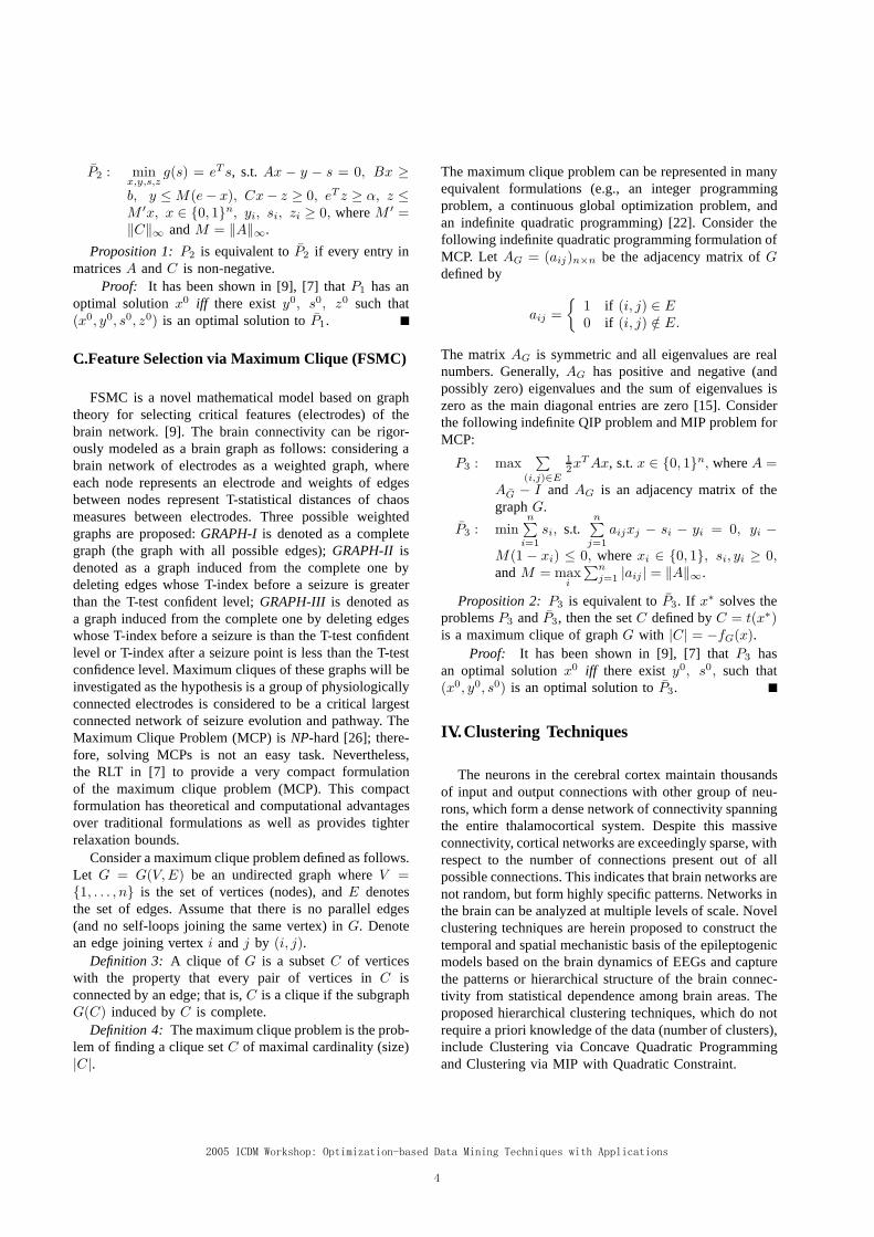
P2 : minx,y,s,z

g(s) = eT s, s.t. Ax − y − s = 0, Bx ≥b, y ≤ M(e − x), Cx − z ≥ 0, eT z ≥ α, z ≤M ′x, x ∈ {0, 1}n, yi, si, zi ≥ 0, where M ′ =‖C‖∞ and M = ‖A‖∞.

Proposition 1: P2 is equivalent to P2 if every entry inmatrices A and C is non-negative.

Proof: It has been shown in [9], [7] that P1 has anoptimal solution x0 iff there exist y0, s0, z0 such that(x0, y0, s0, z0) is an optimal solution to P1.

C.. Feature Selection via Maximum Clique (FSMC)

FSMC is a novel mathematical model based on graphtheory for selecting critical features (electrodes) of thebrain network. [9]. The brain connectivity can be rigor-ously modeled as a brain graph as follows: considering abrain network of electrodes as a weighted graph, whereeach node represents an electrode and weights of edgesbetween nodes represent T-statistical distances of chaosmeasures between electrodes. Three possible weightedgraphs are proposed: GRAPH-I is denoted as a completegraph (the graph with all possible edges); GRAPH-II isdenoted as a graph induced from the complete one bydeleting edges whose T-index before a seizure is greaterthan the T-test confident level; GRAPH-III is denoted asa graph induced from the complete one by deleting edgeswhose T-index before a seizure is than the T-test confidentlevel or T-index after a seizure point is less than the T-testconfidence level. Maximum cliques of these graphs will beinvestigated as the hypothesis is a group of physiologicallyconnected electrodes is considered to be a critical largestconnected network of seizure evolution and pathway. TheMaximum Clique Problem (MCP) is NP-hard [26]; there-fore, solving MCPs is not an easy task. Nevertheless,the RLT in [7] to provide a very compact formulationof the maximum clique problem (MCP). This compactformulation has theoretical and computational advantagesover traditional formulations as well as provides tighterrelaxation bounds.

Consider a maximum clique problem defined as follows.Let G = G(V, E) be an undirected graph where V ={1, . . . , n} is the set of vertices (nodes), and E denotesthe set of edges. Assume that there is no parallel edges(and no self-loops joining the same vertex) in G. Denotean edge joining vertex i and j by (i, j).

Definition 3: A clique of G is a subset C of verticeswith the property that every pair of vertices in C isconnected by an edge; that is, C is a clique if the subgraphG(C) induced by C is complete.

Definition 4: The maximum clique problem is the prob-lem of finding a clique set C of maximal cardinality (size)|C|.

The maximum clique problem can be represented in manyequivalent formulations (e.g., an integer programmingproblem, a continuous global optimization problem, andan indefinite quadratic programming) [22]. Consider thefollowing indefinite quadratic programming formulation ofMCP. Let AG = (aij)n×n be the adjacency matrix of Gdefined by

aij =

{1 if (i, j) ∈ E0 if (i, j) /∈ E.

The matrix AG is symmetric and all eigenvalues are realnumbers. Generally, AG has positive and negative (andpossibly zero) eigenvalues and the sum of eigenvalues iszero as the main diagonal entries are zero [15]. Considerthe following indefinite QIP problem and MIP problem forMCP:

P3 : max∑

(i,j)∈E

12xT Ax, s.t. x ∈ {0, 1}n, where A =

AG − I and AG is an adjacency matrix of thegraph G.

P3 : minn∑

i=1

si, s.t.n∑

j=1

aijxj − si − yi = 0, yi −M(1 − xi) ≤ 0, where xi ∈ {0, 1}, si, yi ≥ 0,and M = max

i

∑n

j=1 |aij | = ‖A‖∞.

Proposition 2: P3 is equivalent to P3. If x∗ solves theproblems P3 and P3, then the set C defined by C = t(x∗)is a maximum clique of graph G with |C| = −fG(x).

Proof: It has been shown in [9], [7] that P3 hasan optimal solution x0 iff there exist y0, s0, such that(x0, y0, s0) is an optimal solution to P3.

IV.. Clustering Techniques

The neurons in the cerebral cortex maintain thousandsof input and output connections with other group of neu-rons, which form a dense network of connectivity spanningthe entire thalamocortical system. Despite this massiveconnectivity, cortical networks are exceedingly sparse, withrespect to the number of connections present out of allpossible connections. This indicates that brain networks arenot random, but form highly specific patterns. Networks inthe brain can be analyzed at multiple levels of scale. Novelclustering techniques are herein proposed to construct thetemporal and spatial mechanistic basis of the epileptogenicmodels based on the brain dynamics of EEGs and capturethe patterns or hierarchical structure of the brain connec-tivity from statistical dependence among brain areas. Theproposed hierarchical clustering techniques, which do notrequire a priori knowledge of the data (number of clusters),include Clustering via Concave Quadratic Programmingand Clustering via MIP with Quadratic Constraint.

A.. Clustering via Concave Quadratic Programming(CCQP)

CCQP is a novel clustering mathematical model usedto formulate a clustering problem as a QIP problem [9].Given n points of data to be clustered, we can formulatea clustering problem as follows: min

xf(x) = xT Ax− λI,

s.t. x ∈ {0, 1}n, where A is an n×n Euclidean matrix ofpairwise distance, I is an identity matrix, λ is a parameteradjusting the degree of similarity within a cluster, xi isa 0-1 decision variable indicating whether or not pointi is selected to be in the cluster. Note that λI is anoffset parameter added to the objective function to avoidthe optimal solution of all xi are zero. This will happenwhen every entry aij of Euclidean matrix A is positiveand the diagonal is zero. Although this clustering problemis formulated as a large QIP problem, in some instanceswhen λ is large enough to make the quadratic functionbecome concave function, this problem can be convertedto a continuous problem (minimizing a concave quadraticfunction over a sphere) [9]. The reduction to a continuousproblem is the main advantage of CCQP. This propertyholds because of the fact that a concave function f : S → over a compact convex set S ⊂ n attains its globalminimum at one of the extreme points of S [15]. Twoequivalent forms of CCQP problems are given by:

P4 : minx

f(x) = xT Ax, s.t. x ∈ {0, 1}n, where A isan n × n Euclidean matrix

P4 : minx

f(x) = xT Ax, s.t. 0 ≤ x ≤ e, where A =

A + λI , λ is any real number, I is a diagonalmatrix.

Proposition 3: P4 is equivalent to P4.

Proof: We will demonstrate that P2 has an optimalsolution x0 iff x0 is an optimal solution to P2 as follows.If we choose λ such that A = A+ λI becomes a negativesemidefinite matrix (e.g., λ = −μ, where μ is the largesteigenvalue of A), then the objective function f(x) becomesconcave and the constraints can be replaced by 0 ≤ x ≤e. Thus, discrete problem P2 is equivalent to continuousproblem P2 [9].

One of the advantages of CCQP is the ability to systemat-ically determine the optimal number of clusters. AlthoughCCQP has to solve m clustering problems iteratively(where m is the final number of clusters at the terminationof CCQP algorithm), it is efficient enough to solve large-scale clustering problems because only one continuousproblem is solved in each iteration. After each iteration,the problem size will become significantly smaller [9].Figure 1 presents the procedure of CCQP.

CCQPInput: All n unassigned data points in set S

Output: The number of clusters and cluster assignmentfor all n data points

WHILE S �= ∅ DO- Construct an Euclidean matrix A from

pair-wise distance of data points in S

- Solve CCQP in problem P4

IF Optimal solution xi = 1 THEN- Remove point i from set S

Fig. 1. Procedure of CCQP algorithm

B.. Clustering via MIP with Quadratic Constraint(CMIPQC)

CMIPQC is a novel clustering mathematical modelin which a clustering problem can be formulated as amixed-integer programming problem with quadratic con-straint [9]. The goal of CMIPQC is to maximize numberof data points to be in a cluster such that the simi-larity degrees among data points in a cluster are lessthan a pre-determined parameter, α. This technique canbe incorporated with hierarchical clustering methods asfollows: (a) Initialization: assign all data points into onecluster; (b) Partition: use CMIPQC to divide the bigcluster into smaller clusters; (3) Repetition: repeat thepartition process until the stopping criterion are reachedor a cluster contains a single point. Novel mathematical

formulation for CMIPQC is given by: maxx

n∑i=1

xi, s.t.

xT Cx ≤ α, x ∈ {0, 1}, where n is the number of datapoints to be clustered, C is an n × n Euclidean matrix ofpairwise distance, α is a predetermined parameter of thesimilarity degree within each cluster, xi is a 0-1 decisionvariable indicating whether or not point i is selected to bein the cluster. The objective of this model is to maximizenumber of data points to be in a cluster such that theaverage pairwise distances among those points are lessthan α. The difficulty of this problem comes from thequadratic constraint; however, this quadratic constraint canbe efficiently linearized by the RLT described in [7]. TheCMIPQC problem is much easier to solve as it can bereduced to an equivalent MIP problem. Similar to CCQP,the CMIPQC algorithm has the ability to systematicallydetermine the optimal number of clusters and only needsto solve m MIP problems (see Figure 2 for CMIPQCalgorithm). Two equivalent forms of CMIPQC are givenby:

P5 : minx

f(x) =n∑

i=1

xi, s.t. xT Cx ≤ α, x ∈ {0, 1}n

P5 : minx

f(x, y, z) =n∑

i=1

xi, s.t. Cx − z ≥ 0, eT z ≥α, z ≤ M ′x, x ∈ {0, 1}n, zi ≥ 0, where M ′ =

‖C‖∞.

Proposition 4: P3 is equivalent to P3.Proof: The proof of P5 has an optimal solution x0

iff there exist z0 such that (x0, z0) is an optimal solutionto P5 as follows. P5 is a special case of P2 is very similarto the one in [9], [7].

CMIPQCInput: All n unassigned data points in set S

Output: The number of clusters and cluster assignmentfor all n data points

WHILE S �= ∅ DO- Construct an Euclidean matrix A from

pair-wise distance of data points in S

- Solve CMIPQC in problem P5

IF Optimal solution xi = 1 THEN- Remove point i from set S

Fig. 2. Procedure of CMIPQC algorithm

V.. Materials and Methods

The data used in our studies consist of continuousintracranial EEGs from 3 patients with temporal lobeepilepsy. FSQIP was previously used to demonstrate thepredictability of epileptic seizures [4]. In this research, weextend our previous findings of the seizure predictabilityby using FSMQIP to select the critical cortical sites. TheFSMQIP problem is formulated as a MQIP problem withobjective function to minimize the average T-index (ameasure of statistical distance between the mean values ofSTLmax) among electrode sites, the knapsack constraintto identify the number of critical cortical sites [18], and anadditional quadratic constraint to ensure that the optimalgroup of critical sites shows the divergence in STLmax

profiles after a seizure. The experiment in this studyis to test the hypothesis that FSMQIP can be used toselect critical features (electrodes) that are mostly likely tomanifest pre-cursor patterns prior to a seizure. The resultsof this study will demonstrate that if one can select criticalelectrodes that will manifest seizure pre-cursors, it maybe possible to predict a seizure in time to warn of animpending seizure [6]. To test this hypothesis, we designedan experiment used to compare the probability of detectingseizure pre-cursor patterns from critical electrodes selectedby FSMQIP with that from randomly selected electrodes.In this experiment, testing on 3 patients with 20 seizures,we randomly selected 5,000 groups of electrodes, and usedFSMQIP to select the critical electrodes. The experimentin this study is conducted as the following steps:

1) The estimation of STLmax profiles [2], [19], [23],[30], [31] is used to measure the degree of order ordisorder (chaos) of the EEG signals.

2) FSMQIP select the critical electrodes based upon thebehavior of STLmax profiles before and after eachpreceding seizure.

3) Such a seizure pre-cursor will be detected when thebrain dynamics from critical electrodes manifest apattern of transitional convergence in the similaritydegree of chaos. This pattern can be viewed as asynchronization of the brain dynamics from criticalelectrodes.

VI.. Results

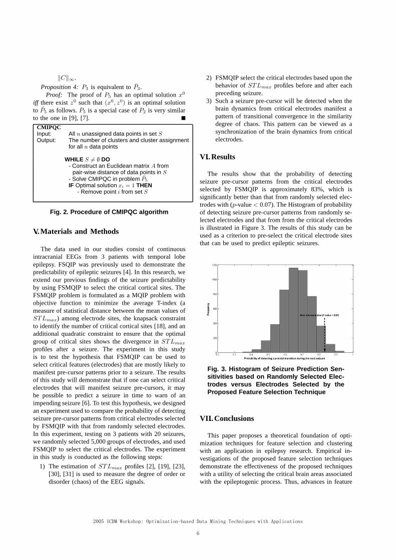
The results show that the probability of detectingseizure pre-cursor patterns from the critical electrodesselected by FSMQIP is approximately 83%, which issignificantly better than that from randomly selected elec-trodes with (p-value < 0.07). The Histogram of probabilityof detecting seizure pre-cursor patterns from randomly se-lected electrodes and that from from the critical electrodesis illustrated in Figure 3. The results of this study can beused as a criterion to pre-select the critical electrode sitesthat can be used to predict epileptic seizures.

Fig. 3. Histogram of Seizure Prediction Sen-sitivities based on Randomly Selected Elec-trodes versus Electrodes Selected by theProposed Feature Selection Technique

VII.. Conclusions

This paper proposes a theoretical foundation of opti-mization techniques for feature selection and clusteringwith an application in epilepsy research. Empirical in-vestigations of the proposed feature selection techniquesdemonstrate the effectiveness of the proposed techniqueswith a utility of selecting the critical brain areas associatedwith the epileptogenic process. Thus, advances in feature

selection and clustering techniques will result in the futuredevelopment of a novel DM paradigm to predict impendingseizures from multichannel EEG recordings. Prediction ispossible because, for the vast majority of seizures, thespatio-temporal dynamical features of seizure pre-cursorsare sufficiently similar to that of the preceding seizure.Mathematical formulations for novel clustering techniquesare also proposed in this paper. These techniques are theo-retically fast and scalable. The results from this preliminaryresearch suggest that empirical studies of the proposedclustering techniques should be investigated in the futureresearch.

References

[1] W. Adams and H. Sherali, “Linearization strategies for a classof zero-one mixed integer programming problems,” OperationsResearch, vol. 38, pp. 217–226, 1990.

[2] A. Babloyantz and A. Destexhe, “Low dimensional chaos in aninstance of epilepsy,” Proc. Natl. Acad. Sci. USA, vol. 83, pp. 3513–3517, 1986.

[3] P. Bradley, O. Mangasarian, and W. Street, “Clustering via con-cave minimization,” in Advances in Neural Information ProcessingSystems, M. Mozer, M. Jordan, and T. Petsche, Eds. MIT Press,1997.

[4] W. Chaovalitwongse, “Optimization and dynamical approaches innonlinear time series analysis with applications in bioengineering,”Ph.D. dissertation, University of Florida, 2003.

[5] W. Chaovalitwongse, L. Iasemidis, P. Pardalos, P. Carney, D.-S. Shiau, and J. Sackellares, “Performance of a seizure warningalgorithm based on the dynamics of intracranial EEG,” EpilepsyResearch, vol. 64, pp. 93–133, 2005.

[6] W. Chaovalitwongse, P. Pardalos, L. Iasemidis, D.-S. Shiau, andJ. Sackellares, “Applications of global optimization and dynamicalsystems to prediction of epileptic seizures,” in Quantitative Neu-roscience, P. Pardalos, J. Sackellares, L. Iasemidis, and P. Carney,Eds. Kluwer, 2003, pp. 1–36.

[7] W. Chaovalitwongse, P. Pardalos, and O. Prokoyev, “Reduction ofmulti-quadratic 0–1 programming problems to linear mixed 0–1programming problems,” Operations Research Letters, vol. 32(6),pp. 517–522, 2004.

[8] W. Chaovalitwongse, O. Prokoyev, and P. Pardalos, “Electroen-cephalogram (EEG) time series classification: Applications inepilepsy,” Annals of Operations Research, vol. To appear, 2005.

[9] W. A. Chaovalitwongse, “A robust clustering technique viaquadratic programming,” Department of Industrial and SystemsEngineering, Rutgers University, Tech. Rep., 2005.

[10] W. A. Chaovalitwongse, P. Pardalos, L. Iasemidis, D.-S. Shiau, andJ. Sackellares, “Dynamical approaches and multi-quadratic integerprogramming for seizure prediction,” Optimization Methods andSoftware, vol. 20(2–3), pp. 383–394, 2005.

[11] W. Chaovalitwongse, P. Pardalos, L. Iasemidis, J. Sackellares, andD.-S. Shiau, “Optimization of spatio-temporal pattern processingfor seizure warning and prediction,” U.S. Patent application filedAugust 2004, Attorney Docket No. 028724–150, 2004.

[12] C. Cherniak, Z. Mokhtarzada, and U. Nodelman, “Optimal-wiringmodels of neuroanatomy,” in Computational Neuroanatomy, G. A.Ascoli, Ed. Humana Press, 2002.

[13] C. Elger and K. Lehnertz, “Seizure prediction by non-linear timeseries analysis of brain electrical activity,” European Journal ofNeuroscience, vol. 10, pp. 786–789, 1998.

[14] F. Glover, “Improved linear integer programming formulations ofnonlinear integer programs,” Management Science, vol. 22, pp. 455–460, 1975.

[15] R. Horst, P. Pardalos, and N. Thoai, Introduction to global opti-mization. Kluwer Academic Publishers, 1995.

[16] L. Iasemidis, P. Pardalos, D.-S. Shiau, W. Chaovalitwongse,K. Narayanan, A. Prasad, K. Tsakalis, P. Carney, and J. Sackellares,“Long term prospective on-line real-time seizure prediction,” Jour-nal of Clinical Neurophysiology, vol. 116(3), pp. 532–544, 2005.

[17] L. Iasemidis, D.-S. Shiau, W. Chaovalitwongse, J. Sackellares,P. Pardalos, P. Carney, J. Principe, A. Prasad, B. Veeramani, andK. Tsakalis, “Adaptive epileptic seizure prediction system,” IEEETransactions on Biomedical Engineering, vol. 5(5), pp. 616–627,2003.

[18] L. Iasemidis, D.-S. Shiau, J. Sackellares, and P. Pardalos, “Tran-sition to epileptic seizures: Optimization,” in DIMACS series inDiscrete Mathematics and Theoretical Computer Science, D. Du,P. Pardalos, and J. Wang, Eds. American Mathematical Society,1999, pp. 55–74.

[19] L. Iasemidis, H. Zaveri, J. Sackellares, and W. Williams, “Phasespace analysis of EEG in temporal lobe epilepsy,” in IEEE Eng.in Medicine and Biology Society, 10th Ann. Int. Conf., 1988, pp.1201–1203.

[20] B. Litt, R. Esteller, J. Echauz, D. Maryann, R. Shor, T. Henry,P. Pennell, C. Epstein, R. Bakay, M. Dichter, and G. Vachtservanos,“Epileptic seizures may begin hours in advance of clinical onset: Areport of five patients,” Neuron, vol. 30, pp. 51–64, 2001.

[21] F. Mormann, T. Kreuz, C. Rieke, R. Andrzejak, A. Kraskov,P. David, C. Elger, and K. Lehnertz, “On the predictability of epilep-tic seizures,” Journal of Clinical Neurophysiology, vol. 116(3), pp.569–587, 2005.

[22] T. Motzkin and E. Strauss, “Maxima for graphs and a new proofsof a theorem turan,” Canadian Journal of Mathematics, vol. 17, pp.533–540, 1965.

[23] N. Packard, J. Crutchfield, and J. Farmer, “Geometry from timeseries,” Phys. Rev. Lett., vol. 45, pp. 712–716, 1980.

[24] P. Pardalos, W. Chaovalitwongse, L. Iasemidis, J. Sackellares, D.-S.Shiau, P. Carney, O. Prokopyev, and V. Yatsenko, “Seizure warningalgorithm based on spatiotemporal dynamics of intracranial EEG,”Mathematical Programming, vol. 101(2), pp. 365–385, 2004.

[25] P. Pardalos and G. Rodgers, “Computational aspects of a branch andbound algorithm for quadratic zero-one programming,” Computing,vol. 45, pp. 131–144, 1990.

[26] P. Pardalos and J. Xue, “The maximum clique problem,” Journalof Global Optimization, vol. 4, pp. 301–328, 1992.

[27] P. Pardalos, V. Yatsenko, J. Sackellares, D.-S. Shiau, W. Chaovalit-wongse, and L. Iasemidis, “Analysis of EEG data using optimiza-tion, statistics, and dynamical system techniques,” ComputationalStatistics & Data Analysis, vol. 44(1–2), pp. 391–408, 2003.

[28] O. Prokopyev, V. Boginski, W. Chaovalitwongse, P. Pardalos,J. Sackellares, and P. Carney, “Network-based techniques in EEGdata analysis and epileptic brain modeling,” in Data Mining inBiomedicine, P. Pardalos and A. Vazacopoulos, Eds. Springer,2005, p. To appear.

[29] M. L. V. Quyen, J. Martinerie, M. Baulac, and F. Varela, “Anticipat-ing epileptic seizures in real time by non-linear analysis of similaritybetween EEG recordings,” NeuroReport, vol. 10, pp. 2149–2155,1999.

[30] P. Rapp, I. Zimmerman, and A. M. Albano, “Experimental studiesof chaotic neural behavior: cellular activity and electroencephalo-graphic signals,” in Nonlinear oscillations in biology and chemistry,H. Othmer, Ed. Springer-Verlag, 1986, pp. 175–205.

[31] F. Takens, “Detecting strange attractors in turbulence,” in Dynamicalsystems and turbulence, Lecture notes in mathematics, D. Rand andL. Young, Eds. Springer-Verlag, 1981.

Fuzzy Support Vector Classification Based on Possibility Theory*

Zhimin Yang1 Yingjie Tian

2 Naiyang Deng

3**

1College of Economics & Management, China Agriculture University, 100083, Beijing, China 2Chinese Academy of Sciences Research Center on Data Technology & Knowledge Economy,

100080, Beijing, China 3College of Science, China Agriculture University, 100083, Beijing, China

Abstract

This paper is concerned with the fuzzy support vector classification in which the type of both the output of the training point and the value of the final fuzzy classification function is triangle fuzzy number. First, the fuzzy classification problem is formulated as a fuzzy chance constrained programming. Then we transform this programming into its equivalence quadratic programming. As a result, we propose fuzzy support vector classification algorithm. In order to show its rationality of the algorithm, a example is presented.Keywords machine learning fuzzy support vector classification possibility measuretriangle fuzzy number

1. INTRODUCTION

Support vector machines (SVMs)

proposed by Vapnik, is a powerful tool for

machine learning (Vapnik 1995 Vapnik

1998 Cristianini 2000 Mangasarian 1999

Deng 2004). It is also one of the most

interesting topics in this field. Lin and Wang

in (Lin, 2002) investigated a classification

problem with fuzzy information, where the

training set is )~,(,),~,( 11 ll yxyxS with

output ),,1(~ ljy j is fuzzy number. This

paper studies this problem in a different way.

We formulate it as a fuzzy chance constrained

programming. Then we transform this

programming into its equivalence quadratic

programming.

Assume that the training points contain

complete fuzzy information, i.e. the sum of

the positive membership degree and negative

membership degree of its output is 1. We

propose a fuzzy support vector classification

algorithm. Given an arbitrary test, its

corresponding output obtained by the

algorithm is a triangle fuzzy number.

2. FUZZY SUPPORT VECTOR

CLASSIFICATION MACHINE

As an extension of positive symbol 1 and

negative symbol -1, we introduce triangle

fuzzy number. Define the corresponding

output by the triangle fuzzy number. For an

input of a training point which belongs to the

positive class with the membership

degree )15.0( , the triangle fuzzy

number is

1 2 3

2 2

( , , )

2( ) 2 2( ) 3 2( ,2 1, ),

0.5 1

y r r r

1

Similarly, for an input of a training point

which belongs to the negative class with the

membership degree )15.0( , the

triangle fuzzy number is

1 2 3

2 2

( , , )

2( ) 3 2 2( ) 2( , 2 1, ),

0.5 1

y r r r

. 2

Thus we use )~,( yx to express a training

point, where y~ is a triangle fuzzy number 1

or 2 .We could use ),(x to express a

training point too, where is

3

Given training set of classification is

)~,(,),~,( 11 ll yxyxS , 4

and nj Rx is usual input, ),,1(~ ljy j is a

triangle fuzzy number (1) or (2). According to

(1) ,(2) and (3), the training set (4) can have

another form

),(,),,( 11 llxxS 5

where jx is same to those in (4), while j is

those in (3) lj ,,1 .

Definition 1 )~,( jj yx in (4) and ),( jjx in (5)

are called as fuzzy training points, lj ,,1 ,

and S and S are called as fuzzy training sets.

Definition 2 Fuzzy training point )~,( jj yx or

),( jjx is called as fuzzy positive point if it

corresponds to (1); similarly, fuzzy training

point )~,( jj yx or ),( jjx is called as fuzzy

negative point if it corresponds to (2).

Note: In this paper, the case either 5.0j

or 5.0j is omitted, because the

corresponding triangle fuzzy

number )2,0,2(~jy can not provide any

information.

We rearrange the fuzzy training points in

fuzzy training set 4 or 5 , such that the

new fuzzy training set

)~,(,),~,(),~,(,),~,( 1111 llpppp yxyxyxyxS6

or

),(,),,(),,(,),,( 1111 llpppp xxxxS 7

has the following property:

)~,( tt yx and ),( ttx are fuzzy positive points

( pt ,,1 ), )~,( ii yx and ),( iix are fuzzy

negative points ( lpi ,,1 ).

Definition 3 Suppose a fuzzy training set (6)

or equivalently (7) and a confidence level

10 .If there exist nRw and

Rb so that

ljbxwyPos jj ,,1}1))((~{

(8

then fuzzy training set (6) or (7)is fuzzy

linearly separable, moreover the

corresponding fuzzy classification problem is

fuzzy linearly separable.

Note: 1 Fuzzy linearly separable can be

considered, roughly speaking, that inputs of

fuzzy positive points and fuzzy negative

points can be separated at least with the

possibility degree )10( .

2 Fuzzy linearly separability is

generalization of linearly separability of usual

training set. In fact, if ),,11 ptt and

),,1(1 lpii in training set (7),

fuzzy training set degenerates to usual

training set. So fuzzy linearly separability of

fuzzy training set degenerates to linearly

separability of usual training set. Supposed

1t ( pt ,,1 ) or

1i ( lpi ,,1 ), it is possible that, on

one hand, pxx ,,1 and lp xx ,,1 are not

linearly separable in usual meaning; on the

other hand, they are fuzzy linearly separable.

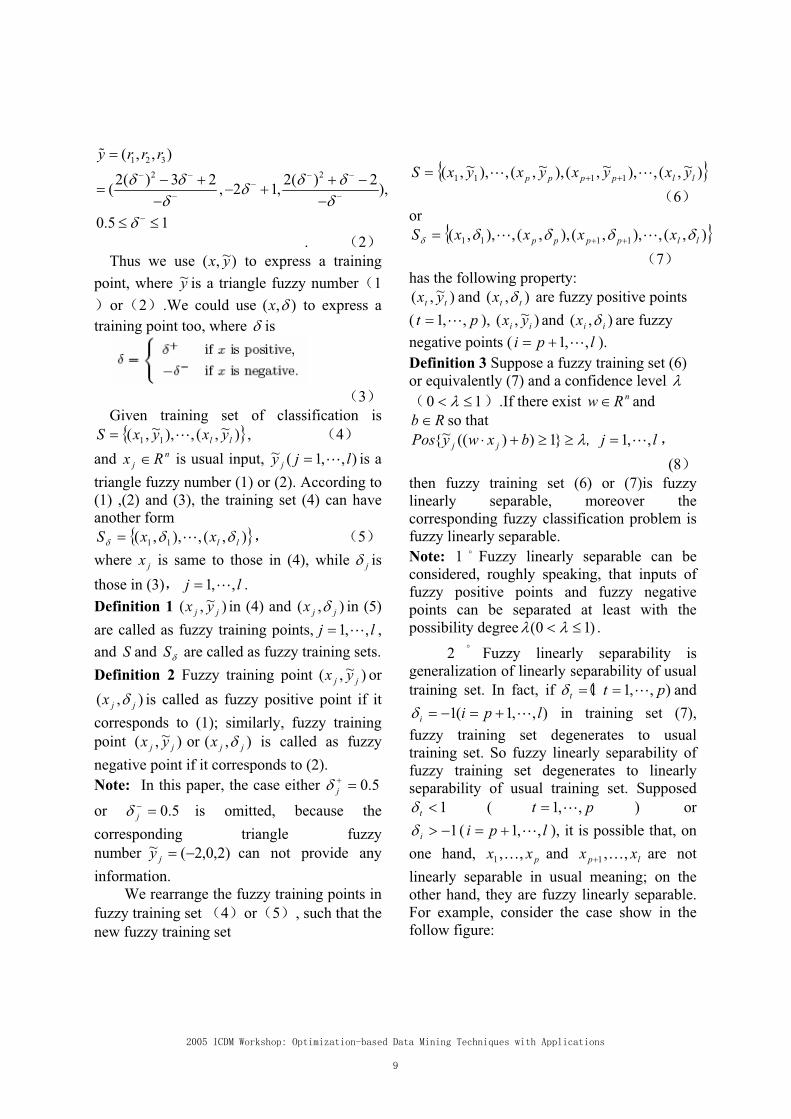
For example, consider the case show in the

follow figure:

13x 0 12x 21x

)1(1 33 y )1(1 22 y 1

Supposed there are three fuzzy training

points ),( 11 yx , ),( 22 yx and ),( 33 yx . The fuzzy

training points ),( 22 yx and ),( 33 yx are

certain with )1(1 22 y and

)1(1 33 y . The first fuzzy training

point ),( 11 yx is fuzzy with two possible

negative membership degrees 51.01 and

6.01 .

51.01 .According to (2), triangle

fuzzy number of ),( 11x is

)9.1,02.0,94.1(~1y .So the fuzzy training

set is )},(),,(),~,{( 332211 yxyxyxS .

Suppose 72.0 , and classification

hyperplane 0x , then 2)( 1 bxw , so

7.0722.0}1))((~{ 11 bxwyPos ,

moreover

7.01}1))(({ 22 bxwyPos7.01}1))((~{ 33 bxwyPos .

Therefore fuzzy training set S is fuzzy

linearly separable in the confidence level

72.0 .

� 6.01 .According to (2), triangle

fuzzy number of ),( 11x is

)13.1,2.0,53.1(~1y .So the fuzzy training

set is )},(),,(),~,{( 332211 yxyxyxS .

Suppose 47.0 , and classification

hyperplane 0x , then 2)( 1 bxw , so

47.047.0}1))((~{ 11 bxwyPos ,

moreover

47.01}1))(({ 22 bxwyPos47.01}1))((~{ 33 bxwyPos .

Therefore fuzzy training set S is fuzzy

linearly separable in the confidence level

47.0 .Supposed 72.0 , we will find no

classification hyperplane such that

72.0}1))((~{ 11 bxwyPos . 9

So fuzzy training set S is not fuzzy

linearly separable in the confidence level 72.0 .

Generally speaking, possibility measure

inequality of fuzzy event can be equivalently

transformed to real inequalities, as shown in

(10).

Theorem 1. (8) in Definition 3 is

equivalent with the real inequalities shown in

:

.,,1,1)))(()1((

,,1,1)))(()1((

21

23

lpibxwrrptbxwrr

iii

ttt

10

Proof: ),,(~321 jjjj rrry is a triangle fuzzy

number, so ))((~1 bxwy jj is also a triangle

fuzzy number due to triangle fuzzy number

operation rule. More concretely,

If 0)( bxw t ,

then

3

2

1

1 (( ) ) (1 (( ) ),

1 (( ) ),

1 (( ) ))

t t t t

t t

t t

y w x b r w x br w x br w x b

pt ,,1 .

According to a triangle fuzzy number

),,(~321 rrra and arbitrary given confidence

level 10 , there exists

21)1(}0~{ rraPos .

Therefore, if 0)( bxw t , then

3

2

{1 (( ) ) 0}

(1 )(1 (( ) ))

(1 (( ) )) 0

1, ,

t t

t t

t t

Pos y w x br w x b

r w x bt p

or 3 2

{ (( ) ) 1}

((1 ) )(( ) ) 1

t t

t t t

Pos y w x br r w x b

pt ,,1 .

Similarly, if 0)( bxw i , then

1 2

{ (( ) ) 1}

((1 ) )(( ) ) 1

i i

i i i

Pos y w x br r w x b

lpi ,,1 .

Therefore (8) in Definition 3 is equivalent

with (10). �

In (10), suppose

ptrr

ktt

t ,,1)1(

1

23

lpirr

lii

i ,,1,)1(

1

21

, 11

then 10 can be rewritten:

.,,1,)(

,,1,)(

lpilbxwptkbxw

ii

tt

Definition 4 Suppose fuzzy linearly

separable problem of fuzzy training set (6) or

(7), the two parallel hyperplanes

kbxw )( and lbxw )( are support

hyperplanes about fuzzy training set (6) or

(7), so that:

.}){(max

,,1,)(

}){(min

,,1,)(

,,1

,,1

lbxwlpilbxw

kbxw

ptkbxw

ilpi

ii

tpt

tt

),,1( ptkt ),,1( lpili is the same

to those in (10 }{min,,1

tptkk

}{max,,1

ilpill .

Distance of two support hyperplanes

kbxw )( and lbxw )( is

||||

||

wlk

and we call the distance with margin

0k and 0l are constant . Due to

essence idea of Support Vector Machine, our

goal is to maximize margin. In the confidence

level )10( , fuzzy linearly separable

problem with fuzzy training set (6)or (7) can

be transformed to fuzzy chance constrained

programming with decision variable Tbw ),,( :

ljbxwyPosts

w

jj

bw

,,1,}1))((~{..

||||2

1min 2

,

12

where Pos is possibility measure of fuzzy

event .

Theorem 2 In the confidence level

)10( , the certain equivalence

programming (usual programming equivalent

with (12) )of fuzzy chance constrained

programming 13 is the quadratic

programming below:

.,,1,1)))(()1((

,,1,1)))(()1.((.

||||2

1min

21

23

2

,

lpibxwrrptbxwrrts

w

iii

ttt

bw

13

Proof: The result can be got directly

with Theorem 1. �

Theorem 3. There exists an optimal

solution of quadratic programming (13).

Proof: omitted. (see Deng 2004)�

We will solve the dual programming of

quadratic programming (13).

Theorem 4. The dual programming of

quadratic programming (13) is quadratic

programming with decision variable is T),( :

,1 1

3 2

1

1 2

1

1min ( 2 ) ( )

2

. . ((1 ) )

((1 ) ) 0

0, 1, ,

0, 1, ,

p l

t it i p

p

t t ttl

i i ii p

t

i

A B C

s t r r

r r

t pi p l

14

where

3 2

1 1

3 2

((1 ) )

*((1 ) )( )

p p

t s t tt s

s s t s

A r r

r r x x

3 2

1 1

1 2

((1 ) )

*((1 ) )( )

p l

t i t tt i p

i i t i

B r r

r r x x

1 2

1 1

1 2

((1 ) )

*((1 ) )( )

l l

i q i ii p q p

q i i q

C r r

r r x xpT

p R),,( 1

plTlp R),,( 1

T),( is

decision variable.

Proof: omitted. (see Deng 2004)�

Programming 14 is convex. After

getting its optimal solution T),( ** ,,,( **

1 pT

lp ), *1

* , we

find a optimal solution Tbw ),( ** of fuzzy

coefficient programming (12) is:

* *

3 2

1

*

1 2

1

((1 ) )

((1 ) )

p

t t t tt

l

i i i ii p

w r r x

r r x

*

3 2

*

3 2

1

*

1 2

1

((1 ) )

((1 ) )( )

((1 ) )( )

s sP

t t t t stl

i i i i si p

b r r

r r x x

r r x x

}0|{ *

sssor

*

2

*

3 2

1

*

1 2

1

((1 ) )

((1 ) )( )

((1 ) )( )

qi q

p

t t t t qtl

i i i i qi p

b r r

r r x x

r r x x

}0|{ *

qqq .

So we can get certain optimal classification

hyperplane(see Deng 2004) : nRxbxw ,0)( ** . (15)

Defining the function:** )()( bxwxg

)1(,1

0)1(),(

)1(,1

)1(0),(

)(

1

1

1

1

uuu

uuu

u , 16

Where )(1 u and )(1 u are

respectively the inverse function of )(uand )(u .

Both )(u and )(u are regression function

(monotonously on u ) obtained by the

following way:

Computation of )(u :

� Construct training set of regression

problem

)}),((,),),({( 11 ppxgxg 17

� Using (17) as training set , and

selecting appropriate 0 , 0C ,

support vector regression machine with

linear kernel are executed.

Computation of )(u :

� Construct training set of regression

problem

)}),((,),),({( 11 llpp xgxg . 18

� Using (13) as training set, and

selecting the same 0 , 0C , support

vector regression machine with linear kernel

are executed.

Note: The equation (11) has the following

explanation: Consider an input x .It seems

natural that the larger )(xg is, the larger the

corresponding membership degree to be a

fuzzy positive point is; the smaller )(xg is,

the larger the corresponding membership

degree to be a fuzzy negative point is. The

regression function )( and )( just reflect

this idea.

The above discussion leads to

Algorithm (fuzzy support vector

classification)

� Given a fuzzy training set (6) or (7)

,and select a appropriate confidence

level )1( , 0C and a kernel

function ),( xxK ,then construct quadratic

programming:

,1 1

3 2

1

1 2

1

1min ( 2 ) ( )

2

. . ((1 ) )

((1 ) ) 0

0 , 1, ,

0 , 1, ,

p l

K K K t it i p

p

t t ttl

i i ii p

t

i

A B C

s t r r

r r

C t pC i p l

18

where

3 2

1 1

3 2

((1 ) )

*((1 ) ) ( , )

p p

K t s t tt s

s s t s

A r r

r r K x x

3 2

1 1

1 2

((1 ) )

*((1 ) ) ( , )

p l

K t i t tt i p

i i t i

B r r

r r K x x

1 2

1 1

1 2

((1 ) )

*((1 ) ) ( , )

l l

K i q i ii p q p

q i i q

C r r

r r K x xpT

p R),,( 1

plTlp R),,( 1

T),( is

decision variable.

� Solve quadratic programming (18),

and get optimal solution T),( ** T

lpp ),,,,,( **

1

**

1 .

� Select ),0(* Cs in* or ),0(* Cq in * then compute

*

3 2

*

3 2

1

*

1 2

1

((1 ) )

((1 ) ) ( , )

((1 ) ) ( , )

s sp

t t t t stl

i i i i si p

b r r

r r K x x

r r K x x

Or*

2

*

3 2

1

*

1 2

1

((1 ) )

((1 ) ) ( , )

((1 ) ) ( , ))

qi q

p

t t t t qtl

i i i i qi p

b r r

r r K x x

r r K x x

.

� Construct function

*

3 2

1

*

1 2

1

( ) ((1 ) ) ( , )

((1 ) ) ( , )

p

t t t ttl

i i i ii p

g x r r K x x

r r K x x.

(�)Consider )}),((,),),({( 11 ppxgxgand )}),((,),),({( 11 llpp xgxg as

training set respectively and construct

regression functions

)(u and )(u by support vector

regression with linear kernel.

� According to (1),(2) and (3), we

transform the function ))(( xg in 16

to triangle fuzzy number ( )y y x , then we

get fuzzy optimal classification function.

Note: 1 If the outputs of all fuzzy training

points in fuzzy training set(6) or (7) are real

number 1 or -1, then fuzzy training set

degenerate to normal training set, so fuzzy

support vector classification machine

degenerate to support vector classification

machine.

2 The selection of confidence level

)10( in fuzzy support vector

classification machine would be seen as

parameter selection problem, so we can use

methods in parameter selection such as LOO

error and LOO error bound (Deng 2004).

3. Numerical Experiments

In order to show the rationality of our

algorithm, we give a simple example.

Suppose fuzzy training set contains three

fuzzy positive points and three fuzzy negative

points. According to (6) and (7), this fuzzy

training set can be expressed:

)}~,(,),~,(),~,(,),~,{( 66443311 yxyxyxyxS,

)},(,),,(),,(,),,{( 66443311 xxxxSTx )2,,2(1

Tx )2,7.1(2

Tx )1,5.1(3

Tx )0,0(4

Tx )5.0,8.0(5

Tx )5.0,1(6

)1,1,1(11y )1,1,1(12y)1.1,6.0,1.0(~

3y )1,1,1(14y)1,1,1(15y

)1.0,6.0,1.1(1~6y 11 12

8.03 14 15

8.06 .

Suppose a confidence

level 8.0 , 10C and kernel

function xxxxK ),( . We use the

Algorithm (fuzzy support vector

classification), so that we get

function 4][2][2)( 21 xxxg .

We will establish function ))(( xg :

Look )}8.0,1(),1,4.3(),1,4{(1S as fuzzy

training set, and select 10,1.0 C and

linear kernel. Construct support vector

regression, and we get regression function

72.008.0)( uu ;

Look )}8.0,1(),1,4.1(),1,4{(2S as

fuzzy training set, and select

10,1.0 C and linear kernel. Construct

support vector regression, and we get

regression function 73.007.0)( uu ;

So we get membership function is:

0.08 ( ) 0.72,0 ( ) 3.50

1, ( ) 3.50( ( ))

0.07 ( ) 0.73, 3.86 ( ) 0

1, ( ) 3.86

g x g xg x

g xg x g x

g x

.

Suppose test points

input TT xx )0,1(,)2,1( 87 , and we get

02)( 7xg 88.0))(( 7xg02)( 8xg 87.0))(( 8xg through

)(xg and ))(( xg . According to

(1),(2)and(3), we can get

)03.1,76.0,49.0(~7y and

)44.0,74.0,9.0(~8y (triangle fuzzy

number).

In order to find relationship and difference

between fuzzy support vector classification

and support vector classification, we will have

three respective outputs of the third fuzzy

training point in fuzzy training set S ,more

concretely, 13 , 8.03 13 .

While output of the sixth fuzzy training point

is 16 , therefore fuzzy training set S will

become three sets respectively:

)},(,),,(),,(,),,{( 66443311

1 xxxxSTx )1,5.1(3 13

Tx )5.0,1(6

16 .The inputs and outputs of other fuzzy

training points is the same to those in S .

)},(,),,(),,(,),,{( 66443311

2 xxxxSTx )1,5.1(3 8.03

Tx )5.0,1(6

16 . The inputs and outputs of other

fuzzy training points is the same to those

in S .

)},(,),,(),,(,),,{( 66443311

3 xxxxSTx )1,5.1(3 13

Tx )5.0,1(6

16 .

The inputs and outputs of other fuzzy

training points is the same to those in S .

So we observe the change of optimal

classification hyperplanes with the variety of

output of the third fuzzy training point:

18.08.01 3333 (19)

When all the outputs of training points in

training set are 1 or -1,fuzzy training set

degenerate to usual training set such as 31 , SS . At the same time, fuzzy support

vector classification degenerates to support

vector classification.

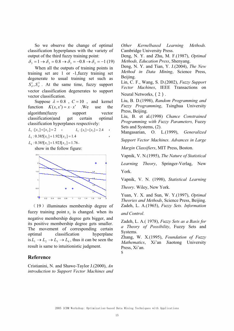
Suppose 8.0 , 10C , and kernel

function xxxxK ),( .We use the

algorithm(fuzzy support vector

classification)and get certain optimal

classification hyperplanes respectively:

2][][: 211 xxL 4.2][][: 212 xxL

4.1][923.1][385.0: 213 xxL

76.1][923.1][385.0: 214 xxL .

show in the follow figure:

0 0.2 0.4 0.6 0.8 1 1.2 1.4 1.6 1.8 20

0.5

1

1.5

2

2.5

L1

L2

L3

L4

19 illuminates membership degree of

fuzzy training point 3x is changed. when its

negative membership degree gets bigger, and

its positive membership degree gets smaller.

The movement of corresponding certain

optimal classification hyperplane

is 4321 LLLL , thus it can be seen the

result is same to intuitionistic judgment.

Reference

Cristianini, N. and Shawe-Taylor J.(2000), Anintroduction to Support Vector Machines and

Other Kernelbased Learning Methods.Cambridge University Press.

Deng, N. Y. and Zhu, M. F.(1987), OptimalMethods, Education Press, Shenyang.

Deng, N. Y. and Tian, Y. J.(2004), The New Method in Data Mining, Science Press,

Beijing.

Lin, C. F., Wang, S. D.(2002), Fuzzy Support Vector Machines, IEEE Transactions on

Neural Networks, 2 .

Liu, B. D.(1998), Random Programming and Fuzzy Programming, Tsinghua University

Press, Beijing.

Liu, B. et al.(1998) Chance Constrained Programming with Fuzzy Parameters, Fuzzy

Sets and Systems, (2).

Mangasarian, O. L.(1999), Generalized

Support Vector Machines. Advances in Large

Margin Classifiers, MIT Press, Boston.

Vapnik, V. N.(1995), The Nature of Statistical

Learning Theory, Springer-Verlag, New

York.

Vapnik, V. N. (1998), Statistical Learning

Theory. Wiley, New York.

Yuan, Y. X. and Sun, W. Y.(1997), OptimalTheories and Methods, Science Press, Beijing.

Zadeh, L. A.(1965), Fuzzy Sets. Information

and Control.

Zadeh, L. A.( 1978), Fuzzy Sets as a Basis for a Theory of Possibility, Fuzzy Sets and

Systems.

Zhang, W. X.(1995), Foundation of Fuzzy Mathematics, Xi’an Jiaotong University

Press, Xi’an. S

Abstract—In order to find the performance improvement

direction for DMU (Decision Making Unit), this paper proposes a

new classification techniques. The proposed method consists of

two stages: (1) DEA (Data Envelopment Analysis) for evaluating

DMUs by their inputs/outputs, (2) GT (Group Technology) for

finding clusters among DMUs. A case study for twelve DMUs with

two inputs and two outputs shows that the proposed technique

works to obtain four clusters where each cluster has its own

performance improvement direction. This paper also discusses

the comparison on the traditional clustering and the proposed

clustering.

Index Terms—Data Envelopment Analysis, Clustering methods,

Data mining, Decision-making, Linear programming.

I. INTRODUCTION

nder the condition that there are a great number of

competitors in a general marketplace, a company should

find out its own advantages compared with others and extend it

[2]. For the reason mentioned above, the concern with the

mathematical approach has been growing [5] [11] [16].

Especially, this paper concentrates on the following issues: (1)

characterize each company in the marketplace by its activity

and define groups by similarity, and (2) compare a company to

others and find the performance improvement direction [3] [4].

As the former issue, in these years, a lot of cluster analyses

have been developed. Cluster analysis is the method for

classification samples which are characterized by multi

property values [5] [6]. It allows us to get common

characteristics in a group, in other words, the reason why a

sample belongs to a group. However, the traditional analysis

calculation regards all property values as appositional.

Therefore, it often gets rules which are based on absolute

property values, and makes difficult to find the performance

Manuscript received October 1, 2005, DEA-based Classification for Finding

Performance Improvement Direction.

S. Aoki is with the Graduate School of Engineering, Osaka Prefecture

University, 1-1 Gakuencho, Sakai, Osaka 599-8531, Japan (corresponding

author to provide phone: +81-72-254-9354; fax: +81-72-254-9915; e-mail:

aoki@cs.osakafu-u.ac.jp)

Y. Nishiuchi is with the Graduate School of Engineering, Osaka Prefecture

University, 1-1 Gakuencho, Sakai, Osaka 599-8531, Japan (e-mail:

nisiuti@cs.osakafu-u.ac.jp)

H. Tsuji is with the Graduate School of Engineering, Osaka Prefecture

University, 1-1 Gakuencho, Sakai, Osaka 599-8531, Japan (e-mail:

tsuji@cs.osakafu-u.ac.jp)

improvement direction for each sample.

As the other issue, DEA has been developed and applied a

variety of the managerial and economic problem situations [8].

By comparison with Pareto optimal solution so called

"efficiency frontier", performance of DMUs is measured

relatively. However, in other words, DEA has considered only

a part of DMUs which used to form the efficiency frontier.

Therefore, little attention has been given to the cluster

technique for classification all DMUs.

In order to improve these problems, this paper proposes a

new classification techniques. The proposed method consists of

two stages: (1) DEA for evaluating DMUs by their

inputs/outputs, (2) GT for finding clusters among DMUs.

The remaining structure of this paper is organized as

follows: section 2 describes about DEA as the basis of this

research. Section 3 proposes the DEA based classification

method. Section 4 illustrates a numerical simulation using the

proposal method and the traditional method, and discusses the

difference between their classification results. Section 5 obtains

universal prospects of two methods. Finally, conclusion and

future extensions are summarized in section 6.

II. DATA ENVELOPMENT ANALYSIS (DEA)

A. An overview on DEA Data Envelopment Analysis, initiated by Charnes et al.

(1978) [7], has been widely applied to efficiency (productivity)

analysis, and more than fifteen hundreds of researches have

been performed in the past twenty years [8].

DEA assumes DMUs activity that uses multiple inputs to

yield multiple outputs, and defines the process which changes

multiple inputs into multiple outputs as “efficiency score”. By

comparison with Pareto optimal solution so called "efficiency

frontier", efficiency score of DMU is measured relatively.

B. Efficiency frontier This section illustrates efficiency frontier visually using

an exercise with a sample data set. In Figure 1, suppose that

there are seven DMUs which have one input and two outputs

where X-axis is an amount of sales (output 1) over a number of

shops (input) and Y-axis is a number of visitors (output 2) over

a number of shops (input). So, if a DMU is located in

upper–right region, it shows that the DMU has high

productivity.

Line B-C-F-G is efficiency frontier in Figure 1. The

DMUs on this frontier are considered that an “efficient”

DEA-based Classification for Finding

Performance Improvement Direction

Shingo Aoki, Member, IEEE, Yusuke Nishiuchi, Non-Member, Hiroshi Tsuji, Member, IEEE

U

activity is done. Other DMUs are considered that an

“inefficient” activity is done and there are rooms to improve

their activities.

For instance, the DMUE’s efficiency score equals to

OE/OE1. Thus the range of efficiency score is [0, 1]. The

efficiency score for DMUB, DMUC, DMUF, and DMUE are

equal to 1.

Number of visitors per number of shops

Am

ou

nt

of

sale

s p

er n

um

ber

of

Sh

op

s

A

B

C

F

GE

D

Efficiency FrontierA1

E1

Fig. 1. Graphical description of efficiency measurement

C. DEA model When there are n DMUs (DMU1, …, DMUk, …, DMUn),

and each DMU is characterized by its own performance with m

inputs (x1k, x2k,…, xmk) and s outputs (y1k, y2k,…, ysk), DEA

model is mathematically expressed by the following

formulation [11] [12]:

freenj

UL

sryy

mixxtoSubject

Minimize

j

n

jj

rk

n

jjrj

ik

n

jjij

k

:),,...,2,1(0

),...,2,1(

),...,2,1(0

1

1

1

In Formulation (1), L and U are the values of lower bound

and upper bound of then

j j1. If L = 0 and U = ,

Formulation (1) is called “the CCR model”, and if L = U = 1,

Formulation (1) is called “the BCC model”[13] [14] [15]. This

paper used the CCR model.

k is the efficiency score in the manner that k = 1 (100%)

means DMU “efficient”, while k < 1 means “inefficient”.

j (j = 1, 2, , n) can be considered to form the efficiency

frontier about DMUk. Especially, if j > 0, then DMUj is on the

efficiency frontier. A set of these DMU is so called a

“Reference set (Rk)” for the DMUk and expressed as follows:

n}1,...,j0,|{jR jk (2)

Using “Reference Set”, this paper re-defines a set of Rk as a

vector ak which is shown as following:

},...,,{**

2

*

1 nka (3)

In Formulation (1), for instance, when ak = {*

1,…,

*

1v = 0, *

v = 0.7, *

1v ,…, *

1w = 0, *

w = 0.3, *

1w ,…,

*

n = 0} and *

k = 0.85, a reference set of DMUk is { DMUV,

DMUW }. In Fig. 2, the point k’ is nearest point from DMUk on

the efficiency frontier and efficiency value of DMUk shows a

ratio of 1 to 0.85.

0.7

0.3DMUv

DMUw

DMUk

k’

Efficiency frontier

for DMUk

1.0

0.85

Fig.2. Reference set for DMUk

What is important is that this research obtains the segment

connecting the origin with k’ not by researchers’ subjectivities

but by the intention which makes the efficiency of DMUk as

well as possible. The efficiency score of DMUk+1 is obtained

by replacing “k” with “k+1” at Formulation (1).

III. DEA-BASED CLASSIFICATION METHOD

Let us propose the method which consists of the following

steps:

A: Divine a data set into input items or output items.

B: For each DMU, solve formula (1) for getting the

efficiency score and the j values. Then we will get a

similarity coefficient matrix S.

C: Apply rank order algorithm to the similarity coefficient

matrix. Then we will get clusters.

A. Select input and output itmes For the first step, there is a guideline to define a data set as

follows [9]:

1. Each data is numeric, and its value is more than zero,

2. In order to show the feature of DMU’s activity, analyst

should be divined a data set into input items or output items,

3. As for the input item, analyst should choose the data which is

used for the investment such as amount of capital stock,

number of employee, and amount of advertisement invest,

4. As for the output item, analysis should choose the data which

is used for the return such as amount of sales, and number of

visitors,

(1)

B. Create similarity coefficient matrix As the second step, the proposal method calculates an

efficiency score ( k ) for each DMUk in Formula (1), and a

vector ak in formula (3). Then the proposal method creates

similarity coefficient matrix S as follows:

},,,{ n21 aaaS (4)

C. Classify DMUs by rank order algorithm As the last step, DMUs are classified into some groups by

Group Technology (GT) [18], handling the similarity

coefficient matrix S. In this classification, rank order algorithm

by King, J. R [19] is employed. The rank order algorithm

consists of four steps as follows:

1. Step GOTO

weight,ascendingby rows Arrange else

STOP. by weight,order ascendingin are rows If4. Step

2 row,each of weight totalCalculate3. Step

weight,ascendingby columns Arrange2. Step

2column,each of weight totalCalculate1. Step

jij

ji

iij

ij

Mw

Mw

IV. A CASE STUDY

In order to verify the availability of the proposal method,

let us illustrate a numerical simulation.

A. A data set A sample data set is shown in Table 1. The data set

concerns on regards the performance of 12 DMU (DMUA, …,

DMUL), and each DMU has four data items: number of

employee, number of shops, number of visitors and amount of

sales.

B. Traditional cluster analysis B.1. METHOD OF CLUSTERING ANALYSIS. Cluster analysis is an

exploratory data analysis method which aims at sorting

different objects into groups in a way that the degree of

association between objects are maximal if they belong to the

same group and minimal otherwise[5] [20].

Table .DATA SET FOR NUMERICAL STUDIES

DMU

Entity

Number of

employees

Number of

shops

Number of visitors

(K person/month)

Amount of sales

(M /month)

A 10 8 23 21

B 26 10 37 32

C 40 15 80 68

D 35 28 76 60

E 30 21 23 20

F 33 10 38 41

G 37 12 78 65

H 50 22 68 77

I 31 15 48 33

J 12 10 16 36

20 12 64 23

45 26 72 35

Inputs Outputs

The degree of association is estimated by the distance

which is calculated by Ward’s method [21].

Ward’s method is distinct from other methods because it

uses an analysis of variance approach to evaluate the distances

between clusters. When a new cluster c is created by combining

cluster a and cluster b, for example, a distance between cluster

x and cluster c is mathematically expressed by the following

formulation:

2222

abcx

xxb

cx

bxxa

cx

axxc d

nnnd

nnnnd

nnnnd

.cluster in sindividual ofnumber the:

. and cluster between distance a:

mnnmd

m

mn

In general, this method is computationally simple, while it

tends to create small size of clusters.

B2. CLASSIFICATION RESULT. The result of classification for the

data set with Ward’s clustering method obtains a dendrogram

(See Fig. 3). Dendrogram is also called tree diagram.

In Fig.3, when the two individuals have combined together

on the left, it is concerned that the two individuals belong to the

same group.

The final number of clusters depends on the position where

the dendrogram is cut off. To get four clusters, for example, (A,

J, E), (B, F, I), (K, L) and (C, G, D, H) are obtained by cutting

the dendrogram at (1) in Figure 3.

Cut off (1)

(distance among DMUs)

Cut off (2)DMU

Fig.3. Dendrogram by Ward-method

From this classification result and Table 1, the feature of

each group is considered as follows:

(i) Group (A, J, E) is considered as that consists of “small

scale” DMUs,

(ii) Group (B, F, I) is considered as that consists of “lower

middle scale” DMUs,

(iii) Group (K, L) is considered as that consists of “larger

middle scale” DMUs and that a visitor unit price is very

low,

(iv) Group (C, G, D, H) is considered as that consists of

“large scale” DMUs.

(5)

Fig.4 is illustrated the classification analysis by the traditional

method.

Small scaleSmall scale

Lower middle scaleLower middle scale

Larger middle scale

A visitor unit price is very low.

Larger middle scale

A visitor unit price is very low.

Large scaleLarge scale

Numbers of employees

and number of shops

Number of visitors

and amount of sales

Fig.4. Traditional classification result

V. DEA-BASED CLASSIFICATION

This section describes the process of the proposal method.

Step1: Select inputs and outputs. According to Step 1 in

Section 3, the number of employee and the number of shops are

selected as input values, and the number of visitors and the

amount of sales are selected as output values.

Step2: Create a similarity coefficient matrix. By

Formulation (1), (3) and (4), the similarity coefficient matrix S

is obtained as shown in Table .

TABLE II.

SIMILARITY COEFFICIENT MATRIX S

A B C D E F G H I J K L

A 1 1 0 0 0 0 0 0 0 0 0 0 0

B 0.674 0 0 0 0 0 0 0.404 0 0 0.124 0.054 0

C 0.943 0 0 0 0 0 0 0.889 0 0 0.21 0.113 0

D 0.885 1 0 0 0 0 0 0 0 0 0 0.265 0

E 0.331 0 0 0 0 0 0 0.007 0 0 0.38 0.256 0

F 0.757 0 0 0 0 0 0 0.631 0 0 0 0 0

G 1 0 0 0 0 0 0 1 0 0 0 0 0

H 0.755 0 0 0 0 0 0 0.789 0 0 0.715 0 0

I 0.638 0 0 0 0 0 0 0.276 0 0 0.184 0.368 0

J 1 0 0 0 0 0 0 0 0 0 1 0 0

K 1 0 0 0 0 0 0 0 0 0 0 1 0

L 0.556 0 0 0 0 0 0 0.103 0 0 0.176 0.956 0

DMUak

A B C D E F G H I J K L

A 1 1 0 0 0 0 0 0 0 0 0 0 0

B 0.674 0 0 0 0 0 0 0.404 0 0 0.124 0.054 0

C 0.943 0 0 0 0 0 0 0.889 0 0 0.21 0.113 0

D 0.885 1 0 0 0 0 0 0 0 0 0 0.265 0

E 0.331 0 0 0 0 0 0 0.007 0 0 0.38 0.256 0

F 0.757 0 0 0 0 0 0 0.631 0 0 0 0 0

G 1 0 0 0 0 0 0 1 0 0 0 0 0

H 0.755 0 0 0 0 0 0 0.789 0 0 0.715 0 0

I 0.638 0 0 0 0 0 0 0.276 0 0 0.184 0.368 0

J 1 0 0 0 0 0 0 0 0 0 1 0 0

K 1 0 0 0 0 0 0 0 0 0 0 1 0

L 0.556 0 0 0 0 0 0 0.103 0 0 0.176 0.956 0

DMUak

Let us note S in Table . The j values of DMUA, DMUG,

DMUJ and DMUK on efficiency frontier are more than zero,

and at least one of the other DMUs is equal to zero. This means

that the each DMU is characterized by combination of

“efficient” DMUs’ features.

The proposal method is focused attention on such DEA

contribution, and finds the performance improvement direction

for each DMU.

Step3: Classify DMUs by rank order algorithm. The rank

order algorithm for the similarity coefficient matrix S generates

classification as shown in Fig. 5.

The matrix S in Fig. 5 is expressed as follows:

If Sij > 0, then it is considered that there is relevance in

DMUI and DMUJ, the entry is 1.

If Sij = 0, then it is considered that there is no relevance in

DMUI and DMUJ, the entry is empty.

Initial state

Final state

ha

nd

ling

Fig. 5. Classification demonstration by rank order algorithm

Then, four clusters: (A, D), (B, C, E, I, K, L), (F, G, H) and

(J) are obtained as shown in Fig.5. The feature of each group is

considered as follows:

(i) group (A, D) is considered as that consists of DMUs

which get many visitors and large amount of sales by a

few employee and a few shops,

(ii) group (B, C, E, I, K, L) is considered as that consists of

DMUs whose employees are clever in marquee,

(iii) group (F, G, H) is considered as that consists of DMUs

which are managed with large-sized shops,

(iv) group (J) is considered as that consists of DMU which has

many visitors who purchase a lot.

From the above analysis, Fig. 6 is illustrated as a

conceptual diagram which shows the situation of the

classification.

B

D

E

F

J

H

Brand Side

Profit Side

Shop Scale Side

A

BC

D

H

I

K

G

L

Marquee Side

Get large sales with

a few visitor.

Get many visitors

with a few employee.

Get many visitors

and large sales with

many employees

get many visitors and

large amount of sales

in a few employee and

shops.

Fig.6. Proposal classification result

VI. DISCUSSION

From the result of section 4.2, two characteristics by

clustering analysis are considered as follows:

(a) Classification result is based on the scale of management,

(b) The number of clusters can be assigned according to the

purpose.

Therefore, the traditional method does not require

preparation in advance. However, there are demerits that it is

difficult to find the performance improvement direction for a

DMU, since the classification result is only based on scale of

management.

On the other hand, DEA-based classification has three

characteristics as follows:

(a) Classification result is based on the direction of

management,

(b) The number of groups which classified is the same

number of “efficient” DMUs,

(c) Every group has at least one “efficient” DMU.

Since the j values in the similarity coefficient matrix S

(TABLE ) are positive only if the DMU is “efficient”, (b) is

true. As shown in Figure 5, since there is one “efficient” DMU

in every classified group, (c) is also true.

Then, the merits and the demerits of the proposal method

are described. It is easy to find the performance improvement

direction for a DMU. For example, even if a DMU is evaluated

“inefficient”, it is possible to refer the feature of the “efficient”

DMU which belongs to the same group. However, it is

necessary to select right input and right output for preparation.

VII. CONCLUSIONS AND FUTURE EXTENSIONS

This paper has described issues of the traditional

classification method and proposed a new classification

method which finds performance improvement direction. Case

study has shown that the classification by cluster analysis was

based on the scale of management, and that, on the other hand,

the classification by the proposal method was based on the

direction of management.

Future extensions of this research include as follows:

(a) Application for a large scale practical problem,

(b) Meaning assigning method for the derived groups,

(c)Investigating reliability of the performance improvement

direction,

(d) Establishment of the one-step application for the proposed

method.

REFERENCES

[1] Y. Hirose et al, Brand value evaluation paper group report, the Ministry of

Economy, Trade and Industry, 2002.

[2] Y. Hirose et al, Brand value that on-balance-ization is hurried, weekly

economist special issue, Vol.24, 2001.

[3] S. Aoki, Y. Naito, and H. Tsuji, “DEA-based Indicator for performance

Improvement”, Proceeding of The 2005 International Conference on

Active Media Technology, 2005.

[4] Y. Taniguchi, H. Mizuno and H. Yajima, “Visual Decision Support

System”, Proceeding of IEEE International Conference on Systems, Man

and Cybernetics (SCM97), 1997, pp.554-558.

[5] S. Miyamoto, Fuzzy sets in information retrieval and cluster analysis,

Kluwer Academic Publishers, Dordrecht: Boston, 1990.

[6] M.R. Anderberg, Cluster analysis for applications, Academic Press, New

York, USA, 1973.

[7] A. Charnes, W.W. Cooper, and E. Rhodes, “Measuring the efficiency of

decision-making units”, European journal of operational research, vol.2,

1978, pp.429-444.

[8] T. Sueyoshi, Management Efficiency Analysis (in Japanese), Asakura

Shoten Co., Ltd, Tokyo, 2001.

[9] K. Tone, Measurement and Improvement of Management Efficiency (in

Japanese), JUSE Press, Ltd, Tokyo, 1993.

[10] M.J. Farrell, “The Measurement of Productive Efficiency”, Journal of the

Royal Statical Society, (Series A), vol.120, 1957, pp.253-281.

[11] D.L, Adolphson, G.C. Cornia, and L.C. Walters, “A Unified Framework

for Classifying DEA Models”, Operational Research ’90, edited by

E.E.Bradley, Pergamon Press, 1991, pp.647-657.

[12] A. Boussofiane, R.G. Dyson, and E. Thanassoulis, “Invited Review:

Applied Data Envelopment Analysis”, European Journal of Operational

Research, vol.52, 1991, pp-1-15.

[13] R. D. Banker, and R.C. Morey, “The use of categorical variables in Data

Envelopment Analysis”, Management Science vol.32, 1984,

pp.1613-1627

[14] R.D. Banker, A. Charnes, and W.W. Cooper, “Some models for

estimating technical and scale inefficiencies in data envelopment

analysis”, Management Science, Vol.30, 1984, pp.1078-1092.

[15] R.D. Banker, “Estimating Most Productive Scale Size Using Data

Envelopment Analysis”, European Journal of Operational Research,

vol.17, 1984, pp.35-44.

[16] W.A. Kamakura, “A note on the use of categorical variables in Data

Envelopment Analysis”, Management Science, vol.34, 1988,

pp.1273-1276.

[17] [J.J. Rousseau, and J. Semple, “Categorical outputs in Data Envelopment

Analysis”, Management Science, vol.39, 1993, pp.384-386.

[18] J.R. King, V. Nakornchai, “Machine-component group formation in

group technology: review and extension”, Internat. J. Prod, vol.20, 1982,

pp.117-133.

[19] J.R. King, “Machine-Component Grouping in Production Flow Analysis:

An Approach Using a Rank Order Clustering Algorithm”, International

Journal of Production Research, vol. 18, 1980, pp.213-232.

[20] J.G. Hirschberg, and D.J. Aigner, “A Classification for Medium and

Small Firms by Time-of-Day Electricity Usage”, Papers and Proceedings

of the Eight Annual North American Conference of the International

Association of Energy Economists, 1986, pp.253-257.

[21] J. Ward, “Hierarchical grouping to optimize an objective function”,

Journal of the American Statistical Association, vol.58, 1963,

pp.236-244.

Abstract—This paper proposes a decision support method for

the measuring the productivity efficiency based on DEA (Data

Envelopment Analysis). The decision support method, called

Multi-Viewpoint DEA model which integrates the efficiency

analysis and the inefficiency analysis, is possible to identify the

performance of DMU (Decision Making Unit) between the strong

points and weak points by changing the view parameter. A case

study for twenty-five Japanese baseball players shows that the

proposed model is robust of the evaluation value.

Index Terms—Data Envelopment Analysis, Decision-Making,

Linear programming, Productivity.

I. INTRODUCTION

EA [1] is a nonparametric method for finding the relative

efficiency of DMUs, each of which is a company

responsible for converting multiple inputs into multiple outputs.

DEA has been applied to a variety of managerial and economic

problem situations in both public and private sectors [5, 9, 13,

14]. DEA defines the process which changes multiple inputs

into multiple outputs as one evaluation value.

The decision method based on DEA induces two kinds of

approaches: One is the efficiency analysis based on the Pareto

optimal solution for the aspect only of the strong points [1, 5].

The other is the inefficiency analysis based on the Pareto

optimal solution for the aspect only of the weak points [7].

Then, the evaluation values in two approaches are inconsistent

[8]. However, analysts have evaluated DMUs only by extreme

aspect: either strong points or weak points. Thus, the traditional

two analyses lack flexibility and robustness [17].

In fact, while there are many inputs and outputs in DEA

framework, these items are not fully used in the previous

approaches. This type of DEA problem has been usually

tackled by multiplier restriction approaches [15] and cone ratio

Manuscript received September 28, 2005, Multi-Viewpoint Data

Envelopment Analysis for Finding Efficiency and Inefficiency.

S. Aoki is with the Graduate School of Engineering, Osaka Prefecture

University, 1-1 Gakuencho, Sakai, Osaka 599-8531, Japan (corresponding

author to provide phone: +81-72-254-9354; fax: +81-72-254-9915; e-mail:

aoki@cs.osakafu-u.ac.jp)

K. Minami is with the Graduate School of Engineering, Osaka Prefecture

University, 1-1 Gakuencho, Sakai, Osaka 599-8531, Japan

H. Tsuji is with the Graduate School of Engineering, Osaka Prefecture

University, 1-1 Gakuencho, Sakai, Osaka 599-8531, Japan (e-mail:

tsuji@cs.osakafu-u.ac.jp)

approaches [16]. While such multiplier restrictions usually

reduce the number of zero weight, they often produce an

infeasible solution in DEA. Therefore, new DEA model which

has robustness on the evaluation values is required.

This paper proposes a decision support technique referred

to as Multi-Viewpoint DEA model. The remaining structure of

this paper is organized as follows: the next section reviews the

traditional DEA models. Section 3 proposes a new model. The

proposed model integrates the efficiency analysis and the

inefficiency analysis into one mathematical formulation, and

allows us to analyze the performance of DMU by

multi-viewpoint between the strong points and weak points.

Section 4 verifies the proposed model through a case study. A

case study shows that the proposed model has two desirable

features: (1) robustness of the evaluation value, and (2)

unification between efficiency analysis and inefficiency

analysis. Finally, conclusion and future study are summarized

in section 5.

II. DEA-BASED EFFICIENCY AND INEFFICIENCY ANALYSES

A. DEA: Data Envelopment Analysis In order to describe the mathematical structure of the

evaluation value, this paper assumes that there are n DMUs

),DMU,,DMU,,DMU( nk1 where each DMU is

characterized by m inputs )x,,x,,x( mkikk1 and s outputs

).y,,y,,y( skrkk1 Evaluation value of is mathematically

formulated by

mkmk22k11

sksk22k11

k xvxvxv

yuyuyu

DMUof

ValueEvaluation (1)

Here ru is multiplier weight given to the thr output, and

iv is multiplier weight given to the thi input. From the

analysis concept, there are two decision methods for

calculating these weights. One is the efficiency analysis

based on the Pareto optimal solution for the aspect only of

the strong points [1, 5]. The other is the inefficiency analysis

based on the Pareto optimal solution for the aspect only of

the weak points [7, 8].

Fig 1 visually represents the difference of two methods.

Suppose that there are nine DMUs which have one input and

two outputs where X-axis is output 1 over input and Y-axis is

Multi-Viewpoint Data Envelopment Analysis for

Finding Efficiency and Inefficiency

Shingo AOKI, Member, IEEE, Kiyosei MINAMI, Non-Member, Hiroshi TSUJI, Member, IEEE

D

output 2 over input. So, if DMU is located in upper-right

region, it shows that the DMU has high productivity.

Efficiency analysis finds out the efficiency frontier which

indicates the best practice line (B-C-D-E-F in Figure 1) and

evaluates the relative evaluation value by the aspect only of

the strong points. On the other hand, inefficiency analysis

finds out the inefficiency frontier which indicates the worst

practice line (B-I-H-G-F in Fig 1) and evaluates the relative

evaluation value by the aspect only of the weak points.

Output 1 Input

Inefficiency frontier

Efficiency frontier

A

B C

D

E

FG

H

I

A’

A’’

O

Ou

tpu

t 2

Input

Output 1 Input

Inefficiency frontier

Efficiency frontier

A

B C

D

E

FG

H

I

A’

A’’

O

Ou

tpu

t 2

Input

Fig 1. Efficiency analysis and Inefficiency analysis

B. Efficiency Analysis The efficiency analysis measures the efficiency level of a

specific by relativity comparing its performance to the

efficiency frontier. This paper is based on CCR model [1] while

there are other models [5, 11]. The efficiency analysis can be

mathematically formulated by

0u,0v

3)-(21xv

)n,,2,1j(

2)-(20yuxvs.t.

1)-(2)(yuMax

ri

m

1iiki

s

1rrjr

m

1iiji

Ek

s

1rrkr

(2)

Here formula (2-2) is a restriction condition because the

productivity of all DMUs (formula (1)) becomes 100% or less.

And the objective function (2-1) represents the maximization of

the sum of virtual outputs of kDMU , setting that the virtual

inputs of kDMU is equal to 1 (formula (2-3)). Therefore, the

optimal solution of ( u,v ri ) represents the convenient weight

for kDMU . Especially, the optimal objective function value

indicates the evaluation value ( Ek ) for kDMU . This evaluation

value by the convenient weight is called “efficiency score” in

the manner that %)100(1Ek means the state of efficiency,

while %)100(1Ek means the state of inefficiency.

C. Inefficiency analysis There is another analysis which measures the inefficiency

level of a specific kDMU based on Inversed DEA model [7].

The inefficiency analysis can be mathematically formulated by

0u,0v

3)-(31xv

)n,,2,1j(

2)-(30yuxvs.t.

1)-(3)1

(yuinM

ri

m

1iiki

s

1rrjr

m

1iiji

IEk

s

1rrkr

(3)

Again, formula (3-2) is a restriction condition because the

productivity of all DMU (formula (1)) becomes 100% or more.

And the objective function (3-1) represents the minimization of

the virtual outputs of kDMU , setting that the virtual inputs of

kDMU is equal to 1 (formula (3-3)). Therefore, the optimal

solution of ( u,v ri ) represents the inconvenient weight for

kDMU . Especially, the inverse number of optimal objective

function value indicates the “inefficiency score” in the manner

that %)100(1IEk means the state of inefficiency, while

%)100(1IEk means the state of efficiency.

D. Requirement for Multi-Viewpoint DEA As shown in Figure 1, BDMU and FDMU are evaluated

as both states of “efficiency ( 1Ek )” and “inefficiency

)1( IEk ”. This result clearly shows mathematical difference in

two analyses. For the example, BDMU has the best

productivity for the Output 2 / input, while it has worst

productivity for the Output 1 / input. In efficiency analysis, the

weight of BDMU is evaluated by the aspect of the strong points.

Therefore, the weight of Output 2 / input becomes a positive

value and the weight of Output 1 / input becomes zero. On the

other hand, in inefficiency analysis, the weight of BDMU is

evaluated by the aspect of the weak points. Therefore, the

weight of Output 2 / input becomes zero and the weight of

Output 1 / input becomes a positive value. This difference of

the weight estimation causes the mathematical problems as

follow:

a) No robustness of evaluation value

Both analyses may produce zero weights for most inputs

and outputs. The zero weight indicates that the corresponding

inputs or outputs are not used for the evaluation value.

Moreover, if the specific inputs or output items are removed

from the analysis, the evaluation value may change greatly [17].

This type of DEA problem is usually tackled by multiplier

restriction approaches [15] and cone ratio approaches [16].

Such multiplier restrictions usually reduce the number of zero

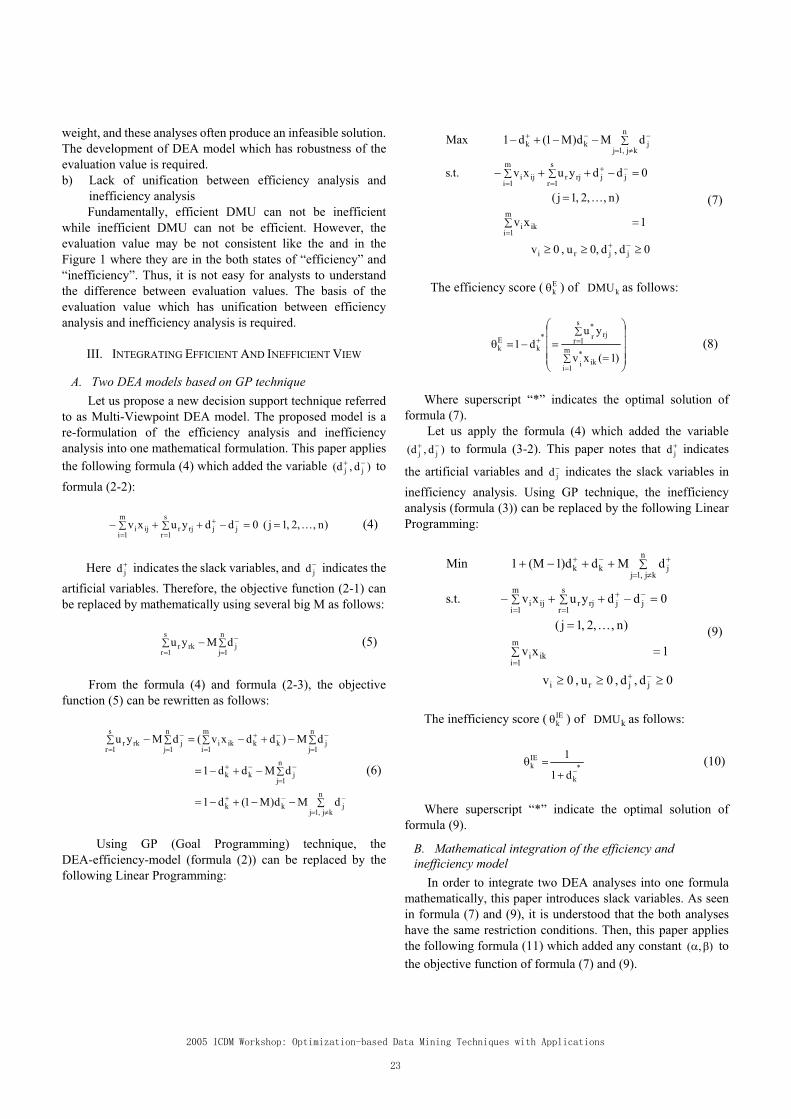
weight, and these analyses often produce an infeasible solution.

The development of DEA model which has robustness of the

evaluation value is required.

b) Lack of unification between efficiency analysis and

inefficiency analysis

Fundamentally, efficient DMU can not be inefficient

while inefficient DMU can not be efficient. However, the

evaluation value may be not consistent like the and in the

Figure 1 where they are in the both states of “efficiency” and

“inefficiency”. Thus, it is not easy for analysts to understand

the difference between evaluation values. The basis of the

evaluation value which has unification between efficiency

analysis and inefficiency analysis is required.

III. INTEGRATING EFFICIENT AND INEFFICIENT VIEW

A. Two DEA models based on GP technique Let us propose a new decision support technique referred

to as Multi-Viewpoint DEA model. The proposed model is a

re-formulation of the efficiency analysis and inefficiency

analysis into one mathematical formulation. This paper applies

the following formula (4) which added the variable )d,d( jj to

formula (2-2):

)n,,2,1j(0ddyuxv jj

s

1rrjr

m

1iiji (4)

Here jd indicates the slack variables, and jd indicates the

artificial variables. Therefore, the objective function (2-1) can

be replaced by mathematically using several big M as follows:

n

1jj

s

1rrkr dMyu (5)

From the formula (4) and formula (2-3), the objective

function (5) can be rewritten as follows:

n

kj,1jjkk

n

1jjkk

n

1jjkk

m

1iiki

n

1jj

s

1rrkr

dMd)M1(d1

dMdd1

dM)ddxv(dMyu

(6)

Using GP (Goal Programming) technique, the

DEA-efficiency-model (formula (2)) can be replaced by the

following Linear Programming:

0d,d,0u,0v

1xv

)n,,2,1j(

0ddyuxv.t.s

dMd)M1(d1Max

jjri

m

1iiki

jj

s

1rrjr

m

1iiji

n

kj,1jjkk

(7)

The efficiency score ( Ek ) of kDMU as follows:

)1(xv

yu

d1m

1iik

*

i

s

1rrj

*

r*

kEk (8)

Where superscript “*” indicates the optimal solution of

formula (7).

Let us apply the formula (4) which added the variable

)d,d( jj to formula (3-2). This paper notes that jd indicates

the artificial variables and jd indicates the slack variables in

inefficiency analysis. Using GP technique, the inefficiency

analysis (formula (3)) can be replaced by the following Linear

Programming:

0d,d,0u,0v

1xv

)n,,2,1j(

0ddyuxv.t.s

dMdd)1(M1inM

jjri

m

1iiki

jj

s

1rrjr

m

1iiji

n

kj,1jjkk

(9)

The inefficiency score ( IEk ) of kDMU as follows:

*

k

IEk

d1

1 (10)

Where superscript “*” indicate the optimal solution of

formula (9).

B. Mathematical integration of the efficiency and inefficiency model In order to integrate two DEA analyses into one formula

mathematically, this paper introduces slack variables. As seen

in formula (7) and (9), it is understood that the both analyses

have the same restriction conditions. Then, this paper applies

the following formula (11) which added any constant ),( to

the objective function of formula (7) and (9).

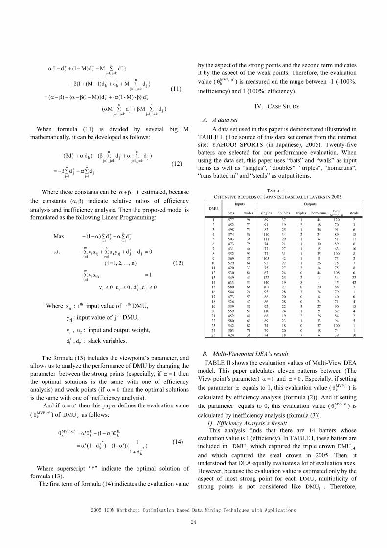
)dMdM(

d}-M)-(1{d)}M1({)(

}dMdd)1(M1{

}dMd)M1(d1{

n

kj,1jj

n

kj,1jj

-kk

n

kj,1jjkk

n

kj,1jjkk

(11)

When formula (11) is divided by several big M

mathematically, it can be developed as follows:

n

1jj

n

1jj

n

kj,1jj

n

kj,1jj

-kk

dd

)dd()dd(

(12)

Where these constants can be 1 estimated, because

the constants ),( indicate relative ratios of efficiency

analysis and inefficiency analysis. Then the proposed model is

formulated as the following Linear Programming:

0d,d,0u,0v

1xv

)n,,2,1j(

0ddyuxv.t.s

dd)1(xaM

jjri

m

1iiki

jj

s

1rrjr

m

1iiji

n

1jj

n

1jj

(13)

Where ijx : thi input value of thj DMU,

rjy : input value of thj DMU,

iv , ru : input and output weight,

id , rd : slack variables.

The formula (13) includes the viewpoint’s parameter, and

allows us to analyze the performance of DMU by changing the

parameter between the strong points (especially, if 1 then

the optimal solutions is the same with one of efficiency

analysis) and weak points (if 0 then the optimal solutions

is the same with one of inefficiency analysis).

And if ' then this paper defines the evaluation value

( ',MVPk ) of kDMU as follows:

)

d1

1()'-(1)d(1'

)'1('

*

k

*

k

IEk

Ek

',MVPk

(14)

Where superscript “*” indicate the optimal solution of

formula (13).

The first term of formula (14) indicates the evaluation value

by the aspect of the strong points and the second term indicates

it by the aspect of the weak points. Therefore, the evaluation

value ( ',MVPk ) is measured on the range between -1 (-100%:

inefficiency) and 1 (100%: efficiency).

IV. CASE STUDY

A. A data set A data set used in this paper is demonstrated illustrated in

TABLE I. (The source of this data set comes from the internet

site: YAHOO! SPORTS (in Japanese), 2005). Twenty-five

batters are selected for our performance evaluation. When

using the data set, this paper uses “bats” and “walk” as input

items as well as “singles”, “doubles”, “triples”, “homeruns”,

“runs batted in” and “steals” as output items.

TABLE .

OFFENSIVE RECORDS OF JAPANESE BASEBALL PLAYERS IN 2005

bats walks singles doubles triples homerunsruns

batted insteals

1 577 96 89 37 1 44 120 2

2 452 73 91 19 2 18 70 3

3 498 71 82 25 1 36 91 6

4 574 56 110 34 2 24 89 18

5 503 38 111 29 1 6 51 11

6 473 75 74 21 1 30 89 6

7 431 46 77 27 1 15 63 10

8 552 91 77 31 1 35 100 8

9 569 57 105 42 1 11 73 2

10 529 64 92 22 1 26 75 7

11 420 33 75 27 2 14 75 8

12 530 84 67 24 0 44 108 0

13 549 41 122 25 2 2 34 22

14 633 51 140 19 8 4 45 42

15 580 66 107 27 0 20 88 7

16 544 24 95 28 3 24 79 1

17 473 53 88 20 0 6 40 0

18 526 47 86 28 0 24 71 4

19 559 50 92 22 3 27 90 18

20 559 51 110 24 1 9 62 4

21 452 40 68 19 2 26 84 2

22 580 61 89 23 1 33 94 5

23 542 82 74 18 0 37 100 1

24 503 78 79 20 0 18 74 1

25 424 36 74 18 7 6 39 10

DMUInputs Outputs

B. Multi-Viewpoint DEA’s result TABLE II shows the evaluation values of Multi-View DEA

model. This paper calculates eleven patterns between (The

View point’s parameter) 1 and 0 . Especially, if setting

the parameter equals to 1, this evaluation value ( 1,MVPk ) is

calculated by efficiency analysis (formula (2)). And if setting

the parameter equals to 0, this evaluation value ( 0,MVPk ) is

calculated by inefficiency analysis (formula (3)).

1) Efficiency Analysis’s Result This analysis finds that there are 14 batters whose

evaluation value is 1 (efficiency). In TABLE I, these batters are

included in 1DMU which captured the triple crown 14DMU

and which captured the steal crown in 2005. Then, it

understood that DEA equally evaluates a lot of evaluation axes.

However, because the evaluation value is estimated only by the

aspect of most strong point for each DMU, multiplicity of

strong points is not considered like 1DMU . Therefore,

superiority can not be applied between these batters in this

analysis.

2) Inefficiency Analysis’s Result This analysis finds that there are 10 batters whose evaluation

value is -1 (inefficiency). Because the evaluation value is

estimated only by the aspect of weak points, these batters are

included in the batters which have a little steals even if

excelling in the long hits like 12DMU and 23DMU . As well as

efficiency analysis, superiority can not be applied between

these batters.

3) Proposed Model’s Result The proposed model allows to analyze the performance of

DMU between efficiency and inefficiency. To clarify the

change of the evaluation value when the view point’s parameter

is shifted from 1 to 0, let us not focus on evaluation value but

on rank. Fig 2 shows the change of rank for the specific four

batters ( 12DMU , 13DMU , 14DMU , 25DMU ) which estimated

the both states of “efficiency” and “inefficiency”.

a) Robustness of the evaluation value Although 25DMU has high rank (25) in the case ( 1 ),

the rank of 25DMU is rapidly lower in the other cases. Where,

thinking about strong points, in TABLE I, it is understood that

it has the superiority for the ratio of doubles (output) / bats

(input). However, the other ratios are not excellent respect.

That is to say, 25DMU has a limited strong point. Oppositely,

as seen in TABLE II, for the batters who is as almighty like

1DMU and 2DMU , the rank does not change easily. Because

the proposed model allows us to know whether DMU has the

multiplicity or limit of strong points, it is possible to evaluate

the DMU with robustness.

b) Unification between DEA-efficiency and DEA-inefficiency model

In the case ( 1, 0.8, 0.7, 0.4, 0.2), the rank of 14DMU

are changed to 25, 12, 19, 11 and 24. Thus, the change of the

rank is large. As shown in TABLE I, because 14DMU has the

multiplicity of strong points such as singles, triples and steals, it

is understood that 14DMU has high rank roughly. However,

this result indicates that the rank does not change linear from

the aspect of strong to weak points. Although the efficiency

analysis and the inefficiency analysis are integrated into one

mathematical formulation, how to assign the view point’s

parameter still remains.

TABLE II.

PARAMETER AND ESTIMATION VALUE ( MVPk )

=1 =0.9 =0.8 =0.7 =0.6 =0.5 =0.4 =0.3 =0.2 =0.1 =0

1 1 0.787 0.592 0.414 0.226 0.043 -0.138 -0.320 -0.504 -0.695 -0.931

2 1 0.805 0.606 0.422 0.231 0.052 -0.135 -0.315 -0.491 -0.634 -0.988

3 1 0.801 0.605 0.419 0.228 0.048 -0.144 -0.327 -0.502 -0.696 -0.890

4 1 0.803 0.610 0.417 0.226 0.045 -0.143 -0.328 -0.509 -0.661 -0.846

5 1 0.800 0.609 0.412 0.220 0.035 -0.158 -0.350 -0.526 -0.656 -0.881

6 0.980 0.749 0.557 0.373 0.196 0.021 -0.172 -0.355 -0.543 -0.720 -0.933

7 0.989 0.743 0.553 0.381 0.185 0.012 -0.184 -0.377 -0.569 -0.718 -0.909

8 0.981 0.683 0.499 0.319 0.150 -0.034 -0.209 -0.405 -0.604 -0.793 -1

9 1 0.710 0.507 0.353 0.159 -0.023 -0.218 -0.405 -0.603 -0.732 -0.963

10 0.947 0.746 0.559 0.373 0.197 0.012 -0.187 -0.377 -0.555 -0.733 -0.930

11 1 0.803 0.612 0.423 0.228 0.037 -0.163 -0.349 -0.501 -0.674 -0.905

12 1 0.714 0.515 0.330 0.177 -0.020 -0.211 -0.386 -0.578 -0.799 -1

13 1 0.738 0.557 0.392 0.177 -0.009 -0.198 -0.372 -0.541 -0.701 -1

14 1 0.748 0.554 0.405 0.209 0.006 -0.201 -0.376 -0.499 -0.677 -1

15 0.955 0.762 0.563 0.389 0.212 0.022 -0.176 -0.362 -0.550 -0.696 -1

16 1 0.797 0.570 0.398 0.216 0.011 -0.185 -0.377 -0.545 -0.722 -0.922

17 0.851 0.640 0.445 0.277 0.126 -0.054 -0.239 -0.427 -0.622 -0.802 -1

18 0.926 0.716 0.520 0.359 0.165 -0.029 -0.213 -0.409 -0.609 -0.787 -1

19 1 0.758 0.573 0.383 0.182 -0.006 -0.198 -0.385 -0.558 -0.733 -0.935

20 0.926 0.729 0.527 0.373 0.176 -0.012 -0.207 -0.406 -0.587 -0.716 -0.946

21 1 0.764 0.570 0.377 0.176 -0.009 -0.197 -0.382 -0.572 -0.744 -0.961

22 0.934 0.731 0.539 0.353 0.172 -0.017 -0.209 -0.404 -0.588 -0.773 -0.971

23 0.916 0.696 0.499 0.326 0.161 -0.033 -0.215 -0.411 -0.608 -0.800 -1

24 0.849 0.644 0.456 0.276 0.117 -0.069 -0.251 -0.427 -0.619 -0.806 -1

25 1 0.632 0.451 0.294 0.109 -0.071 -0.252 -0.436 -0.624 -0.805 -1

DMUEstimation Value

=1 =0=0.5

Ran

k

Parameter

0

5

10

15

20

25

No.12

No.13

No.14

No.25

=1 =0=0.5

Ran

k

Parameter

0

5

10

15

20

25

No.12

No.13

No.14

No.25

Fig 2. Rank of four players

V. CONCLUSION

This paper has proposed a new decision support method,

called Multi-Viewpoint DEA model which integrated the

efficiency analysis and the inefficiency analysis by one

mathematical formulation. The proposed model allows us to

analyze the performance of DMU by changing the view point’s

parameter between the strong points (especially, if 1 then it

becomes efficiency analysis) and weak points (if 0 then it

becomes inefficiency analysis). Regarding twenty-five

Japanese baseball players as DMUs, a case study has shown

that the proposed model has two desirable features: (a)

robustness of the evaluation value, and (b) unification between

efficiency analysis and inefficiency analysis. For the future

study, we will also analytically compare our method to the

traditional approaches [15, 16] and explore how to set the view

point’s parameter.

REFERENCES

[1] A.Charnes, W.W.Cooper, and E.Rhodes, “Measuring the efficiency of

decision making units”, European Journal of Operational Research, 1978,

Vol.2, pp429-444.

[2] T. Sueyoshi and S. Aoki, “A use of a nonparametric statistic for DEA

frontier shift: the Kruskal and Wallis rank test”, OMEGA: The

International Journal of Management Science, Vol.29, No.1, 2001,

pp1-18.

[3] T.Sueyoshi, K.Onishi, and Y.Kinase, “A Bench Mark Approach for

Baseball Evaluation”, European Journal of Operational Research,

Vol.115, 1999, pp.429-428.

[4] T. Sueyoshi, Y. Kinase and S. Aoki, “DEA Duality on Returns to Scale in

Production and Cost Analysis”, Proceedings of the Sixth Asia Pacific

Management Conference 2000, 2000, pp1-7.

[5] W. W. Cooper, L. M. Seiford, K. Tone, Data Envelopment Analysis: A

comprehensive text with models, applications, references and

DEA-Solver software, Kluwer Academic Publishers, 2000.

[6] R. Coombs, P. Sabiotti and V. Walsh, Economics and Technological

Change, Macmillan, 1987.

[7] Y. Yamada, T. Matui and M. Sugiyama, "An inefficiency measurement

method for management systems", Journal of Operations Research

Society of Japan, vol. 37, 1994, pp. 158-168 (In Japanese).

[8] Y. Yamada, T. Sueyoshi, M. Sugiyama, T. Nukina and T. Makino “The

DEA Method for Japanese Management: The Evaluation of Local

Governmental Investments to the Japanese Economy”, Journal of the

Operations Research Society of Japan, Vol.38, No.4, 1995, pp.381-396.

[9] S. Aoki, K. Mishima, H. Tsuji: Two-Staged DEA model with Malmquist

Index for Brand Value Estimation, The 8th World Multiconference on

Systemics, Cybernetics and Informatics, Vol. 10, pp.1-6, 2004.

[10] R. D. Banker, A. Charnes, W. W. Cooper, “Some Models for Estimating

Technical and Scale Inefficiencies in Data Envelopment Analysis”,

Management Science, Vol.30, 1984, pp.1078-1092.

[11] R. D. Banker, and R. M. Thrall, “Estimation of Returns to Scale Using

Data Envelopment Analysis”, European Journal of Operational Research,

Vol.62, 1992, pp.74-82.

[12] H. Nakayama, M. Arakawa, Y. B. Yun, Data Envelopment Analysis in

Multicriteria Decision Making”,M. Ehrgott and X. Gandibleux (eds.)

Multiple Criteria Optimization: State of the Art Annotated Bibliographic

Surveys, Kluwer Acadmic Publishiers, 2002.

[13] E. W. N. Bernroider, V. Stix , “The Evaluation of ERP Systems Using

Data Envelopment Analysis”, Information Technology and Organizations,

Idea Group Pub, 2003, pp.283-286.

[14] Y. Zhou, Y. Chen, “DEA-based Performance Predictive Design of

Complex Dynamic System Business Process Improvement”, Proceeding

of Systems, Man and Cybernetics, 2003. IEEE International Conference,

2003, pp.3008-3013.

[15] R. G. Thompson, L. N. Langemeier, C. T. Lee, and R. M. Thrall, “The

Role of Multiplier Bounds in Efficiency Analysis with Application to

Kansas Farming”, Journal of Econometrics, Vol.46, 1990, pp.93-108.

[16] W. W. Cooper, W. Quanling and G. Yu, “Using Displaced Cone

Representation in DEA models for Nondominated Solutions in

Multiobjective Programming”, Systems Science and Mathematical

Sciences, Vol.10, 1997, pp.41-49.

[17] S. Aoki, Y. Naito, and H. Tsuji, “DEA-based Indicator for performance

Improvement”, Proceeding of The Third International Conference on

Active Media Technology, 2005, pp.327-330.

Abstract—In this study, we utilize the genetic algorithm (GA)

to mine high quality stocks for investment. Given the

fundamental financial and price information of stocks trading,

we attempt to use GA to identify stocks that are likely to

outperform the market by having excess returns. To evaluate the

efficiency of the GA for stock selection, the return of equally

weighted portfolio formed by the stocks selected by GA is used as

evaluation criterion. Experiment results reveal that the proposed

GA for stock selection provides a very flexible and useful tool to

assist the investors in selecting valuable stocks.

Index Terms—Genetic algorithms; Portfolio optimization;

Data mining; Stock selection

I. INTRODUCTION

N the stock market, investors are often faced with a large

number of stocks. A crucial work of their investment

decision process is the selection of stocks. From a data-mining

perspective, the problem of stock selection is to identify good

quality stocks that are potential to outperform the market by

having excess return in the future. Given the fundamental

accounting and price information of stock trading, it is a

prediction problem that involves discovering useful patterns

or relationship in the data, and applying that information to

identify whether a stock is good quality.

Obviously, it is not an easy task for many investors when

they faced with enormous amount of stocks in the market.

With focus on the business computing, applying artificial

intelligence to portfolio selection and optimization is one way

to meet the challenge. Some research has presented to solve

asset selection problem. Levin [1] applied artificial neural

network to select valuable stocks. Chu [2] used fuzzy multiple

attribute decision analysis to select stocks for portfolio.

Similarly, Zargham [3] used a fuzzy rule-based system to

evaluate the listed stocks and realize stock selection. Recently,

Fan [4] utilized support vector machine to train universal

Manuscript received July 30, 2005. This work was supported in part by the

SRG of City University of Hong Kong under Grant No. 7001806.

Lean Yu is with the Institute of Systems Science, Academy of Mathematics

and Systems Science, Chinese Academy of Sciences, Beijing, 100080, China

(e-mail: yulean@amss.ac.cn).

Kin Keung Lai is with the Department of Management Science, City

University of Hong Kong and is also with the College of Business

Administration, Hunan University, 410082, China (phone: 852-2788-8563;

fax:852-2788-8560; e-mail: mskklai@cityu.edu.hk).

Shouyang Wang is with the Institute of Systems Science, Academy of

Mathematics and Systems Science, Chinese Academy of Sciences, Beijing,

100080, China (e-mail: sywang@amss.ac.cn).

feedforward neural networks to perform stock selection.

However, these approaches have some drawbacks in

solving the stock selection problem. For example, fuzzy

approach [2-3] usually lack learning ability, while neural

network approach [1, 4] has overfitting problem and is often

easy to trap into local minima. In order to overcome these

shortcomings, GA is used to perform this task. Some related

typical literature can be referred to [5-7] for more details.

The main aim of this study is to mine valuable stocks using

GA and test the efficiency of the GA for stock selection. The

rest of the study is organized as follows. Section 2 describes

the mining process based on the genetic algorithm in detail.

Section 3 presents a simulation experiment. And Section 4

concludes the paper.

II. GA-BASED STOCK SELECTION PROCESS

Generally, GA imitates the natural selection process in

biological evolution with selection, crossover and mutation,

and the sequence of the different operations of a genetic

algorithm is shown in the left part of Figure 1. That is, GA is

procedures modeled after genetics and evolution. Genetics

provide the chromosomal representation to encode the

solution space of the problem while evolutionary procedures

are designed to efficiently search for attractive solutions to

large and complex problem. Usually, GA is based on the

survival-of-the-fittest fashion by gradually manipulating the

potential problem solutions to obtain the more superior

solutions in population. Optimization is performed in the

representation rather than in the problem space directly. To

date, GA has become a popular optimization method as they

often succeed in finding the best optimum by global search in

contrast to most common optimization algorithms. Interested

readers can be referred to [8-9] for more details.

The aim of this study is to identify the quality of each stock

using GA so that investors can choose some good ones for

investment. Here we use stock ranking to determine the

quality of stock. The stocks with a high rank are regarded as

good quality stock. In this study, some financial indicators of

the listed companies are employed to determine and identify

the quality of each stock. That is, the financial indicators of

the companies are used as input variables while a score is

given to rate the stocks. The output variable is stock ranking.

Throughout the study, four important financial indicators,

return on capital employed (ROCE), price/earnings ratio (P/E

Ratio), earning per share (EPS) and liquidity ratio are utilized

Mining Valuable Stocks with Genetic

Optimization Algorithm

Lean Yu, Kin Keung Lai and Shouyang Wang

I

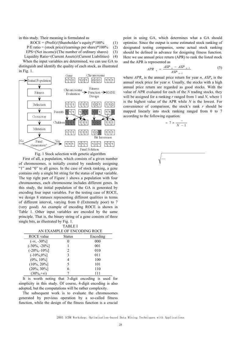
in this study. Their meaning is formulated as

ROCE = (Profit)/(Shareholder’s equity)*100% (1)

P/E ratio = (stock price)/(earnings per share)*100% (2)

EPS=(Net income)/(The number of ordinary shares) (3)

Liquidity Ratio=(Current Assets)/(Current Liabilities) (4)

When the input variables are determined, we can use GA to

distinguish and identify the quality of each stock, as illustrated

in Fig. 1.

Fig. 1 Stock selection with genetic algorithm

First of all, a population, which consists of a given number

of chromosomes, is initially created by randomly assigning

“1” and “0” to all genes. In the case of stock ranking, a gene

contains only a single bit string for the status of input variable.

The top right part of Figure 1 shows a population with four

chromosomes, each chromosome includes different genes. In

this study, the initial population of the GA is generated by

encoding four input variables. For the testing case of ROCE,

we design 8 statuses representing different qualities in terms

of different interval, varying from 0 (Extremely poor) to 7

(very good). An example of encoding ROCE is shown in

Table 1. Other input variables are encoded by the same

principle. That is, the binary string of a gene consists of three

single bits, as illustrated by Fig. 1.

TABLE I

AN EXAMPLE OF ENCODING ROCE

ROCE value Status Encoding

(- , -30%] 0 000

(-30%, -20%] 1 001

(-20%,-10%] 2 010

(-10%,0%] 3 011

(0%, 10%] 4 100

(10%, 20%] 5 101

(20%, 30%] 6 110

(30%,+ ) 7 111

It is worth noting that 3-digit encoding is used for

simplicity in this study. Of course, 4-digit encoding is also

adopted, but the computations will be rather complexity.

The subsequent work is to evaluate the chromosomes

generated by previous operation by a so-called fitness

function, while the design of the fitness function is a crucial

point in using GA, which determines what a GA should

optimize. Since the output is some estimated stock ranking of

designated testing companies, some actual stock ranking

should be defined in advance for designing fitness function.

Here we use annual price return (APR) to rank the listed stock

and the APR is represented as

1

1

n

nnn ASP

ASPASPAPR (5)

where APRn is the annual price return for year n, ASPn is the

annual stock price for year n. Usually, the stocks with a high

annual price return are regarded as good stocks. With the

value of APR evaluated for each of the N trading stocks, they

will be assigned for a ranking r ranged from 1 and N, where 1

is the highest value of the APR while N is the lowest. For

convenience of comparison, the stock’s rank r should be

mapped linearly into stock ranking ranged from 0 to 7

according to the following equation:

17

N

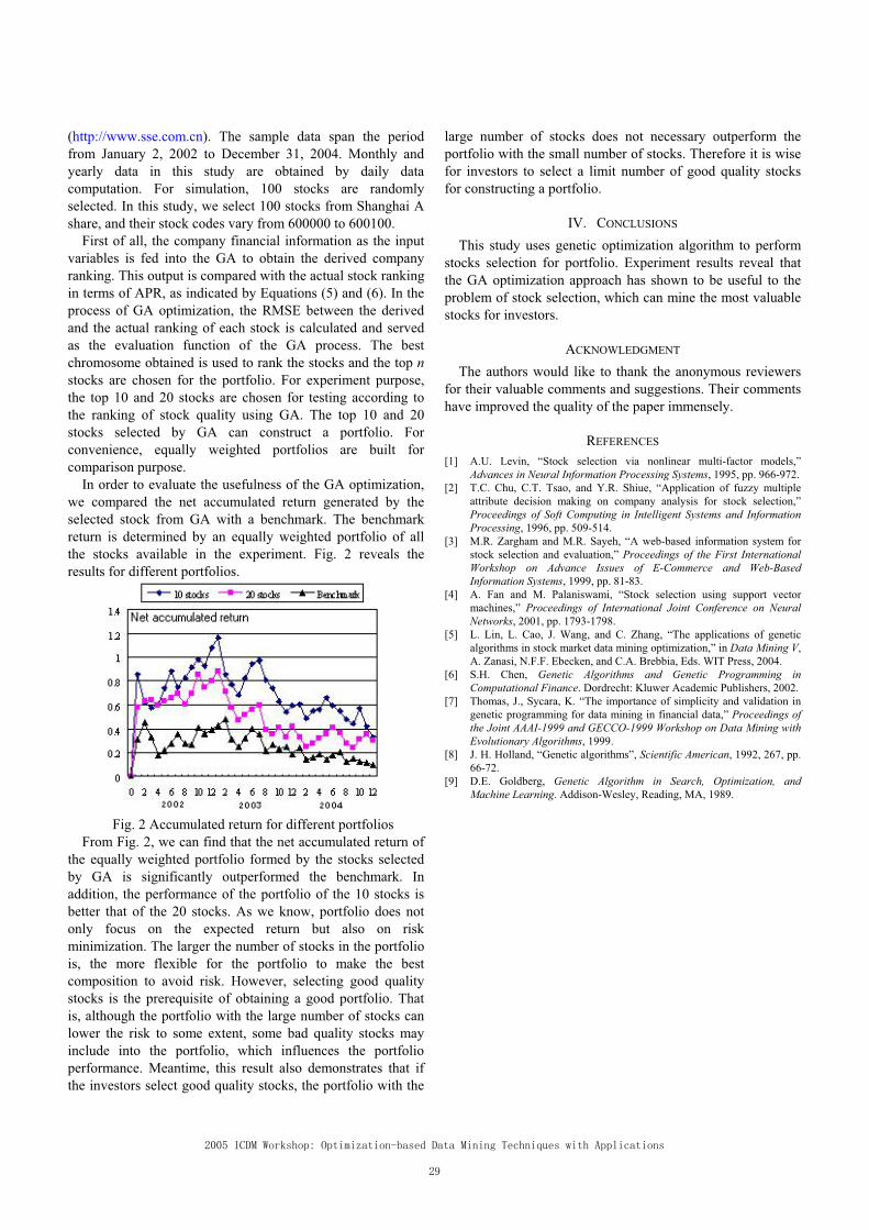
(http://www.sse.com.cn). The sample data span the period

from January 2, 2002 to December 31, 2004. Monthly and

yearly data in this study are obtained by daily data

computation. For simulation, 100 stocks are randomly

selected. In this study, we select 100 stocks from Shanghai A

share, and their stock codes vary from 600000 to 600100.

First of all, the company financial information as the input

variables is fed into the GA to obtain the derived company

ranking. This output is compared with the actual stock ranking

in terms of APR, as indicated by Equations (5) and (6). In the

process of GA optimization, the RMSE between the derived

and the actual ranking of each stock is calculated and served

as the evaluation function of the GA process. The best

chromosome obtained is used to rank the stocks and the top nstocks are chosen for the portfolio. For experiment purpose,

the top 10 and 20 stocks are chosen for testing according to

the ranking of stock quality using GA. The top 10 and 20

stocks selected by GA can construct a portfolio. For

convenience, equally weighted portfolios are built for

comparison purpose.

In order to evaluate the usefulness of the GA optimization,

we compared the net accumulated return generated by the

selected stock from GA with a benchmark. The benchmark

return is determined by an equally weighted portfolio of all

the stocks available in the experiment. Fig. 2 reveals the

results for different portfolios.

Fig. 2 Accumulated return for different portfolios

From Fig. 2, we can find that the net accumulated return of

the equally weighted portfolio formed by the stocks selected

by GA is significantly outperformed the benchmark. In

addition, the performance of the portfolio of the 10 stocks is

better that of the 20 stocks. As we know, portfolio does not

only focus on the expected return but also on risk

minimization. The larger the number of stocks in the portfolio

is, the more flexible for the portfolio to make the best

composition to avoid risk. However, selecting good quality

stocks is the prerequisite of obtaining a good portfolio. That

is, although the portfolio with the large number of stocks can

lower the risk to some extent, some bad quality stocks may

include into the portfolio, which influences the portfolio

performance. Meantime, this result also demonstrates that if

the investors select good quality stocks, the portfolio with the

large number of stocks does not necessary outperform the

portfolio with the small number of stocks. Therefore it is wise

for investors to select a limit number of good quality stocks

for constructing a portfolio.

IV. CONCLUSIONS

This study uses genetic optimization algorithm to perform

stocks selection for portfolio. Experiment results reveal that

the GA optimization approach has shown to be useful to the

problem of stock selection, which can mine the most valuable

stocks for investors.

ACKNOWLEDGMENT

The authors would like to thank the anonymous reviewers

for their valuable comments and suggestions. Their comments

have improved the quality of the paper immensely.

REFERENCES

[1] A.U. Levin, “Stock selection via nonlinear multi-factor models,”

Advances in Neural Information Processing Systems, 1995, pp. 966-972.

[2] T.C. Chu, C.T. Tsao, and Y.R. Shiue, “Application of fuzzy multiple

attribute decision making on company analysis for stock selection,”

Proceedings of Soft Computing in Intelligent Systems and Information Processing, 1996, pp. 509-514.

[3] M.R. Zargham and M.R. Sayeh, “A web-based information system for

stock selection and evaluation,” Proceedings of the First International Workshop on Advance Issues of E-Commerce and Web-Based Information Systems, 1999, pp. 81-83.

[4] A. Fan and M. Palaniswami, “Stock selection using support vector

machines,” Proceedings of International Joint Conference on Neural Networks, 2001, pp. 1793-1798.

[5] L. Lin, L. Cao, J. Wang, and C. Zhang, “The applications of genetic

algorithms in stock market data mining optimization,” in Data Mining V,

A. Zanasi, N.F.F. Ebecken, and C.A. Brebbia, Eds. WIT Press, 2004.

[6] S.H. Chen, Genetic Algorithms and Genetic Programming in Computational Finance. Dordrecht: Kluwer Academic Publishers, 2002.

[7] Thomas, J., Sycara, K. “The importance of simplicity and validation in

genetic programming for data mining in financial data,” Proceedings of the Joint AAAI-1999 and GECCO-1999 Workshop on Data Mining with Evolutionary Algorithms, 1999.

[8] J. H. Holland, “Genetic algorithms”, Scientific American, 1992, 267, pp.

66-72.

[9] D.E. Goldberg, Genetic Algorithm in Search, Optimization, and Machine Learning. Addison-Wesley, Reading, MA, 1989.

A Comparison Study of Multiclass Classification between Multiple Criteria

Mathematical Programming and Hierarchical Method for Support Vector

Machines

Yi Peng1, Gang Kou

1, Yong Shi

1, 2, 3, Zhenxing Chen

1 and Hongjin Yang

2

1College of Information Science & Technology, University of Nebraska at Omaha,Omaha, NE 68182, USA

{ ypeng, gkou, zchen}@mail.unomaha.edu 2Chinese Academy of Sciences Research Center on Data Technology & Knowledge Economy,

Graduate University of the Chinese Academy of Sciences, Beijing 100080, China {yshi, hjyang}@gucas.ac.cn 3The corresponding author

Abstract

Multiclass classification refers to classify data objects into more than two classes. The purpose of this paper is to compare two multiclass classification approaches: Multiple Criteria Mathematical Programming (MCMP) and Hierarchical Method for Support Vector Machines (SVM). While MCMP considers all classes at once, SVM was initially designed for binary classification. It is still an ongoing research issue to extend SVM from two-class classification to multiclass classification and many proposed approaches use hierarchical method. In this paper, we focus on one common hierarchical method – pairwise classification. We compare the performance of MCMP and SVM pairwise approach using KDD99, a large network intrusion dataset. Results show that MCMP achieves better multiclass classification accuracies than SVM pairwise.Keywords: classification, multi-group classification, multi-group Multiple criteria mathematical programming (MCMP), pairwise classification

1. INTRODUCTION

As one of the major data mining

functionalities, classification has broad

applications such as credit card portfolio

management, medical diagnosis, and fraud

detection. Based on historical information,

classification builds classifiers to predict

categorical class labels for unknown data.

Classification methods can be classified in

various ways, and one distinction is between

binary and multiclass classification. Binary

classification, as the name indicates, classifies

data into two classes. Multiclass classification

refers to classify data objects into more than

two classes. Many real-life applications

require multiclass classification. For example,

a multiclass classification that is capable of

predicting subtypes of cancer will be more

helpful than a binary classification that can

only predict cancer or non-cancer.

Researchers have suggested various

multiclass classification methods. Multiple

Criteria Mathematical Programming (MCMP)

and Hierarchical Method for Support Vector

Machines (SVM) are two of them. MCMP

and SVM are both based on mathematical

programming and there is no comparison

study has been conducted to date. The

purpose of this paper is to compare these two

multiclass classification approaches. While

MCMP considers all classes at once, SVM

was initially designed for binary classification.

It is still an ongoing research issue to extend

SVM from two-class classification to

multiclass classification and many proposed

approaches use hierarchical approach. In this

paper, we focus on one common hierarchical

method – pairwise classification. We first

introduce MCMP and SVM pairwise

classification, and then implement an

experiment to compare their performance

using KDD99, a large network intrusion

dataset.

This paper is structured as follows. The

next section discusses the formulation of

multiple-group multiple criteria mathematical

programming classification model. The third

section describes pairwise SVM multiclass

classification method. The fourth section

compares the performance of MCMP and

pairwise SVM using KDD99. The last section

concludes the paper.

2. MULTI-GROUP MULTI-CRITERIA

MATHEMATICAL PROGRAMMING

MODEL

This section introduces a MCMP model

for multiclass classification. Simply speaking,

this method classifies observations into

distinct groups based on two criteria. The

following models represent this concept

mathematically:

Given an r-dimensional attribute

vector ),...,( 1 raaa , let r

irii AAA ),...,( 1 be one of the sample

records, where ;,...,1 ni n represents the total

number of records in the dataset. Suppose k

groups, G1, G2, …, Gk, are predefined.

kjijiGG ji ,1,, and

}...{ 21 ki GGGA , ni ,...,1 . A series

of boundary scalars b1<b2<…<bk-1, can be set

to separate these k groups. The boundary bj is

used to separate Gj and Gj+1. Let X = rT

r Rxx ),...,( 1 be a vector of real number to

be determined. Thus, we can establish the

following linear inequations (Fisher 1936, Shi

et al. 2001):

A i X < b1, A i G1; (1)

bj-1 A i X< bj, A i Gj; (2)

A i X bk-1, A i Gk; (3)

2 j k-1, 1 i n.

A mathematical function f can be used to

describe the summation of total overlapping

while another mathematical

function g represents the aggregation of all

distances. The final classification accuracies

of this multi-group classification problem

depend on simultaneously minimize f and

maximize g . Thus, a generalized bi-criteria

programming method for classification can be

formulated as:

Generalized Model Minimize f and

Maximize gSubject to: (1), (2) and (3)

To formulate the criteria and complete

constraints for data separation, some variables

need to be introduced. In the classification

problem, A i X is the score for the ith data

record. If an element Ai jG is misclassified

into a group other than jG , then let pji,

(p-norm of pji 1,, ) be the Euclidean

distance from A i to bj, and AiX = bj +

ji, , 11 kj and let pji 1, be the

Euclidean distance from A i jG to bj-1, and

AiX = bj-1 - 1, ji , kj2 . Otherwise,

ni1k,j1,, ji , equals to zero.

Therefore, the function f of total overlapping

of data can be represented as k

j

n

ipji

1 1

, .

If an element Ai jG is correctly

classified into jG , let pji, be the

Euclidean distance from A i to bj, and AiX =bj - ji, , 11 kj and let

pji 1, be the

Euclidean distance from A i jG to bj-1, and

AiX = bj-1 + 1, ji , kj2 . Otherwise,

ni1k,j1,, ji , equals to zero. Thus,

the objective is to maximize the distance

pji, from A i to boundary if A i 1G or kG

and is to minimize the distance

pjijj bb

,

1

2from A i to the middle of

two adjunct boundaries bj-1 and bj if

A i 12, kjG j . So the function g of

the distances of every data to its class

boundary or boundaries can be represented as

orkj

n

ipji

1 1

, -1

2 1

,

1

2

k

j

n

ipji

jj bb.

Furthermore, to transform the generalized

bi-criteria classification model into a single-

criterion problem, weights w > 0 and w > 0

are introduced for )(f and )(g ,

respectively. The values of w and w can be

pre-defined in the process of identifying the

optimal solution. As a result, the generalized

model can be converted into a single-criterion

mathematical programming model as:

Model 1 Minimize wk

j

n

ipji

1 1

, - w

(korjj

n

ipji

1 1

, -1

2 1

,

1

2

k

j

n

ipji

jj bb)

Subject to: AiX = bj + ji, - ji, , 11 kj (4)

AiX = bj-1 - 1, ji + 1, ji , kj2 (5)

ji, bj - bj-1 , kj2 (a)

ji, bj+1 - bj , 11 kj (b)

where Ai, i = 1, …, n are given, X and bj are

unrestricted, and ji, , .1,0, niji .

(a) and (b) are defined as such because

the distances from any correctly classified

data (A i 12, kjG j ) to two adjunct

boundaries bj-1 and bj must be less than bj -

bj-1 . A better separation of two adjunct

groups may be achieved by the following

constraints instead of (a) and (b) because (c)

and (d) set up stronger limitation on ji :

ji, (bj - bj-1 )/2+ , kj2 (c)

ji, (bj+1 - bj )/2+ , 11 kj (d)

is a small positive real number.Let p = 2, then objective function in

Model 1 can now be a quadratic objective and

we have:

(Model 2

Minimize wk

j

n

iji

1 1

2

, )( - w

(korjj

n

iji

1 1

2

, )( -

1

2 1

,1

2

, ])()[(k

j

n

ijijjji bb ) (6)

Subject to: (4), (5), (c) and (d)

Note that the constant 21)

2(

jj bbis

omitted from the (6) without any effect to the

solution.

A version of model 2 for three

predefined classes is given in Figure 1. The

stars represent group 1 data objects, the black

dots represent group 2 data objects, and the

white circles represent group 3 data objects.

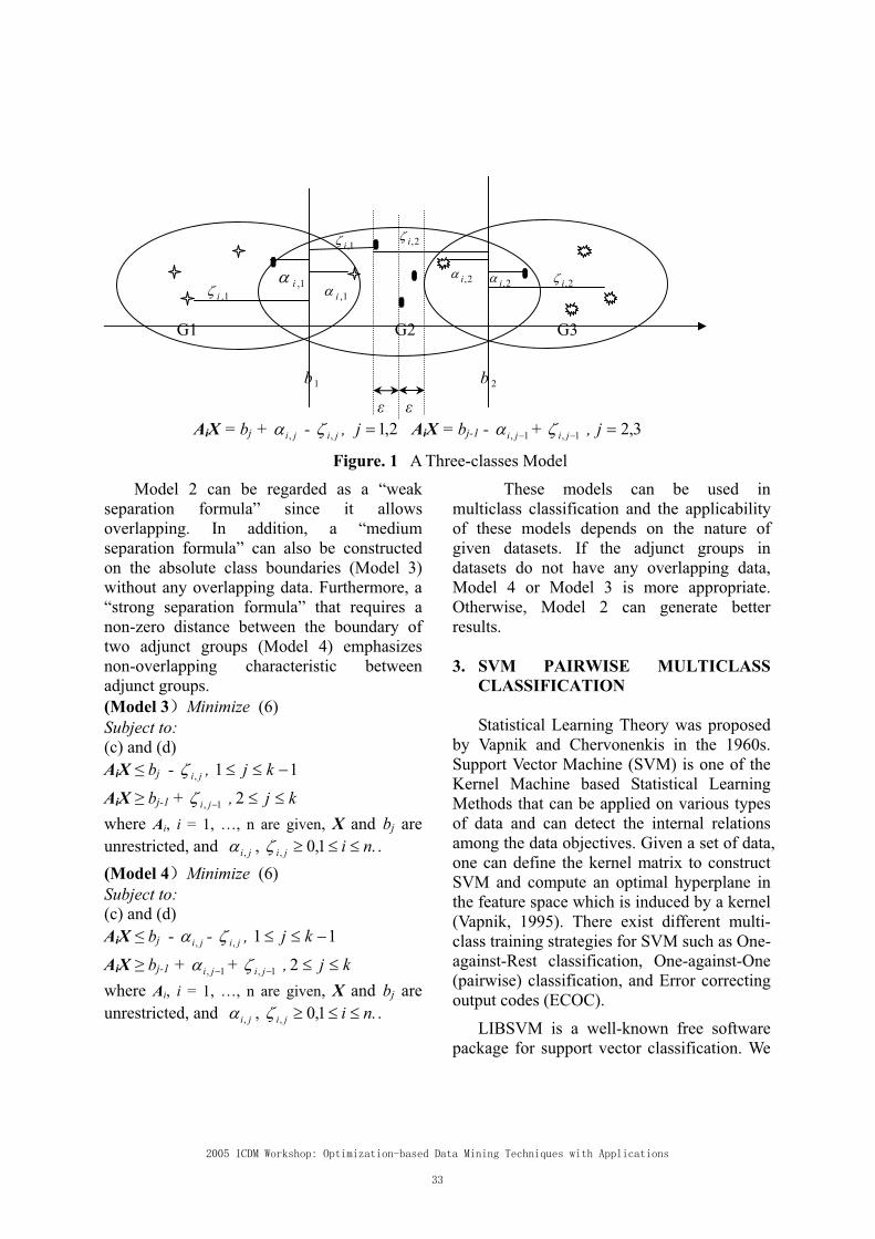
G1 G2 G3

b 1 b 2

AiX = bj + ji, - ji, , 2,1j AiX = bj-1 - 1, ji + 1, ji , 3,2j

Figure. 1 A Three-classes Model

Model 2 can be regarded as a “weak

separation formula” since it allows

overlapping. In addition, a “medium

separation formula” can also be constructed

on the absolute class boundaries (Model 3)

without any overlapping data. Furthermore, a

“strong separation formula” that requires a

non-zero distance between the boundary of

two adjunct groups (Model 4) emphasizes

non-overlapping characteristic between

adjunct groups.

(Model 3 Minimize (6)

Subject to: (c) and (d)

AiX bj - ji, , 11 kj

AiX bj-1 + 1, ji , kj2

where Ai, i = 1, …, n are given, X and bj are

unrestricted, and ji, , .1,0, niji .

(Model 4 Minimize (6)

Subject to: (c) and (d)

AiX bj - ji, - ji, , 11 kj

AiX bj-1 + 1, ji + 1, ji , kj2

where Ai, i = 1, …, n are given, X and bj are

unrestricted, and ji, , .1,0, niji .

These models can be used in

multiclass classification and the applicability

of these models depends on the nature of

given datasets. If the adjunct groups in

datasets do not have any overlapping data,

Model 4 or Model 3 is more appropriate.

Otherwise, Model 2 can generate better

results.

3. SVM PAIRWISE MULTICLASS

CLASSIFICATION

Statistical Learning Theory was proposed

by Vapnik and Chervonenkis in the 1960s.

Support Vector Machine (SVM) is one of the

Kernel Machine based Statistical Learning

Methods that can be applied on various types

of data and can detect the internal relations

among the data objectives. Given a set of data,

one can define the kernel matrix to construct

SVM and compute an optimal hyperplane in

the feature space which is induced by a kernel

(Vapnik, 1995). There exist different multi-

class training strategies for SVM such as One-

against-Rest classification, One-against-One

(pairwise) classification, and Error correcting

output codes (ECOC).

LIBSVM is a well-known free software

package for support vector classification. We

2,i

2,i

2,i1,i

1,i1,i

2,i

1,i

use the latest version, LIBSVM 2.8, in our

experimental study. This software uses one-

against-one (pairwise) method for multiclass

SVM (Chang and Lin, 2001). The one-

against-one method was first proposed by

Knerr et al. in 1990. It constructs totally

2

)1(kk binary SVM classifiers where the

classifiers are trained by two distinct classes

of the total k classes (Hsu and Lin, 2002). The

following quadratic program is used 2

)1(kk

times to generate the multi-category SVM

classifiers.

Min ( /2) || ||2 + (1/2) ||x, b||2

Subject to:

D (AX – eb) e - , where e is a vector of

ones

After2

)1(kk number of SVM classifiers

were produced, a majority vote strategy is

applied to the 2

)1(kk classifiers. Each

classifier has one vote and every data is

predicted to the class with the largest vote.

4. EXPERIMENTAL COMPARISON OF

MCMP AND PAIRWISE SVM

The KDD99 dataset was provided by

Defense Advanced Research Project Agency

(DARPA) in 1998 for the competitive

evaluation of intrusion detection approaches.

KDD 99 dataset contains 9 weeks of raw TCP

data from Simulation of a typical U.S. Air

Force LAN. A version of this dataset was

used in 1999 KDD-CUP intrusion detection

contest (Stolfo et al. 2000). After the contest,

KDD99 has become a de facto standard

dataset for intrusion detection experiments.

There are five main categories of attacks:

denial-of-service (DOS); unauthorized access

from a remote machine (R2L); unauthorized

access to local root privileges (U2R);

surveillance and other probing (Probe).

Because the number of U2R attacks is too

small (52 records), only three types of attacks,

DOS, R2L, and Probe, are used in this

experiment. The KDD99 dataset used in this

experiment has 4898430 records and contains

1071730 distinguish records. MCMP was solved by LINGO 8.0, a software

tool for solving nonlinear models (LINDO

Systems Inc.). LIBSVM version 2.8 (Chang

and Lin, 2001), an integrated software which

uses pairwise approach to support multi-class

SVM classification, was applied to KDD99

data and the classification results of LIBSVM

were compared with MCMP’s.

The four-group classification results of

MCMP and LIBSVM on KDD99 data were

summarized in Table 1 and Table 2,

respectively. The classification results were

displayed in the format of confusion matrices,

which pinpoint the kinds of errors made.

From the confusion matrices in Table 1 and

2, we observe that (1) LIBSVM achieves

perfect classification for training data: 100%

accuracy. The training results of MCMP are

almost perfect: 100% accuracy for “probe”

and “DOS” and 99% accuracy for “normal”

and “R2L”; (2) Contrasted LIBSVM’s

training classification accuracies with testing,

its performance is unstable. LIBSVM

achieves almost perfect classification for

“normal” class: 99.99% accuracy, but poor

performance for three attack types: 44.48%

for “probe”, 53.17% for “R2L”, and 74.49%

for “DOS”. (3) MCMP has a stable

performance on testing data: 97.2% accuracy

for “probe”, 99.07% for “DOS”, 88.43% for

“R2L”, and 97.05% for “normal”.

Table 1. MCMP KDD99 Classification Results

Evaluation on training data (400 cases): Accuracy

False

Alarm

Rate

(1) (2) (3) (4) <-classified as

100 0 0 0 (1): Probe 100.00% 0.99%

0 100 0 0 (2): DOS 100.00% 0.00%

0 0 99 1 (3): R2L 99.00% 0.00%

1 0 0 99 (4): Normal 99.00% 1.00%

Evaluation on test data (1071330 cases):

(1) (2) (3) (4) <-classified as

13366 216 145 24 (1): Probe 97.20% 7.88%

1084 244867 1202 14 (2): DOS 99.07% 6.32%

1 4 795 99 (3): R2L 88.43% 91.86%

59 16313 7623 788718 (4): Normal 97.05% 0.02%

Table 2. LIBSVM KDD99 Classification Results

Evaluation on training data (400 cases): Accuracy

False

Alarm

Rate

(1) (2) (3) (4) <-classified as

100 0 0 0 (1): Probe 100.00% 0.00%

0 100 0 0 (2): DOS 100.00% 0.00%

0 0 100 0 (3): R2L 100.00% 0.00%

0 0 0 100 (4): Normal 100.00% 0.00%

Evaluation on test data (1071330 cases):

(1) (2) (3) (4) <-classified as

6117 569 0 7065 (1): Probe 44.48% 67.84%

12861 184107 0 50199 (2): DOS 74.49% 0.31%

0 0 478 421 (3): R2L 53.17% 6.64%

41 0 34 812638 (4): Normal 99.99% 6.63%

5. CONCLUSION

This is the first time that we investigate the

differences between MCMP and pairwise

SVM for multiclass classification using a

large network intrusion dataset. The results

indicate that MCMP achieves better

classification accuracy than pairwise SVM. In

our future research, we will focus on the

theoretical differences between these two

multiclass approaches.

References

Bradley, P.S., Fayyad, U.M., Mangasarian,

O.L. (1999) Mathematical programming for

data mining: Formulations and challenges.

INFORMS Journal on Computing, 11, 217-

238.

Chang, C. C. and Lin, C. J. (2001) LIBSVM :

a library for support vector machines.

Software available at

http://www.csie.ntu.edu.tw/~cjlin/libsvm.

Hsu, C. W. and Lin, C. J. (2002) A

comparison of methods for multi-class

support vector machines, IEEE Transactions on Neural Networks, 13(2), 415-425.

Knerr, S., Personnaz, L., and Dreyfus, G.

(1990), “Single-layer learning revisited: A

stepwise procedure for building and training a

neural network”, in Neurocomputing:Algorithms, Architectures and Applications, J.

Fogelman, Ed. New York: Springer-Verlag.

Kou, G., Peng, Y., Shi, Y., Chen, Z. and Chen

X. (2004b) “A Multiple-Criteria Quadratic

Programming Approach to Network Intrusion

Detection” in Y. Shi, et al (Eds.): CASDMKM

2004, LNAI 3327, Springer-Verlag Berlin

Heidelberg, 145–153.

LINDO Systems Inc., An overview of LINGO 8.0,

http://www.lindo.com/cgi/frameset.cgi?leftlin

go.html;lingof.html.

Stolfo, S.J., Fan, W., Lee, W., Prodromidis, A.

and Chan, P.K. (2000) Cost-based Modeling

and Evaluation for Data Mining With

Application to Fraud and Intrusion Detection:

Results from the JAM Project, DARPA Information Survivability Conference.

Vapnik, V. N. and Chervonenkis (1964), On

one class of perceptrons, Autom. And Remote Contr. 25(1).Vapnik, V. N. (1995), The Nature of Statistical Learning Theory, Springer, New

York.Zhu, D., Premkumar, G., Zhang, X. and Chu,

C.H. (2001) Data Mining for Network Intrusion Detection: A comparison of Alternativest Methods, Decision Sciences,

Volume 32 No. 4, Fall 2001.

Pattern Recognition for Multimedia CommunicationNetworks Using New Connection Models

between MCLP and SVMJing HE

Institute of Intelligent Informationand Communication Technology

Konan UniversityKobe 658-8501, Japan

Email: hejing@gucas.ac.cn

Wuyi YUEDepartment of Information Science

and Systems EngineeringKonan University

Kobe 658-8501, JapanEmail: yue@konan-u.jp

Yong SHIChinese Academy of Sciences

Research Center on Data Technologyand Knowledge Economy

Beijing 100080, ChinaEmail: yshi@gucas.ac.cn

Abstract— Data mining system of performance evaluation formultimedia communication networks (MCNs) is a challengingresearch and development issue. The data mining system offerstechniques of discovering patterns in voluminous databases. Bymeans of dividing the performance data into usual and unusualcategories, we try to find out the category corresponding to thedata mining system. Many pattern recognition algorithms for thedata mining system have been developed and explored in recentyears such as rough sets, tough fuzzy hybridization, granularcomputing, artificial neural networks, support vector machines(SVM), and multiple criteria linear programming (MCLP). Inthis paper, a new connection model between MCLP and SVM isemployed to identify performance data. In addition to theoreticalfoundations, the paper also includes experiment results. Somereal-time and nontrivial examples for MCNs given in this papershows how MCLP and SVM work and how they can be combinedto be used at the same time in reality. The advantages that everyalgorithm offers are compared with the other methods.

I. INTRODUCTION

Data mining system of performance evaluation for mul-timedia communication networks (MCNs) is a challengingresearch and development issue. The data mining system offerstechniques for discovering patterns in voluminous databases.Fraudulent activity costs the telecommunication industry mil-lions of dollars a year.

It is important to identify potentially fraudulent users andtheir typical usage patterns, and detect their attempts to gainfraudulent entry in order to perpetrate illegal activity. Severalways of identifying unusual patterns can be used such asmultidimensional analysis, cluster analysis and outlier analysis[1].

By means of dividing the performance data into usual andunusual categories, we try to find out the category corre-sponding to the data mining system. Many pattern recognitionalgorithms for data mining have been developed and exploredin recent years such as rough sets, tough fuzzy hybridiza-tion, granular computing, artificial neural Networks, supportvector machines (SVM), multiple criteria linear programming(MCLP) and so on [2].

SVM has been gaining popularity as one of the effectivemethods for machine learning in recent years. In pattern

classification problems with two class sets, SVM generalizeslinear classifiers into high dimensional feature spaces throughnon-linear mappings. The non-linear mappings are definedimplicitly by kernels in the Hilbert space. This means SVMmay produce non-linear classifiers in the original data space.Linear classifiers then are optimized to give the maximalmargins separation between the classes [3]-[5].

Research of linear programming (LP) approach to classifi-cation problems was initiated in [6]-[8]. [9], [10] applied thecompromise solution of MCLP to deal with the same question.

In [11], an analysis for fuzzy linear programming (FLP) inclassification of credit card holder behaviors was presented.During the process of the calculation in [11], we found thatexcept some approaches such as MCLP, SVM, many datamining algorithms try to minimize the influence of outliersor eliminate them altogether.

In other words, the unusual outliers may be of particularinterest, such as in the case of unusual pattern detection,where unusual outliers may indicate fraudulent activities. Thusidentification of usual and unusual patterns is an interestingdata mining task, referred to as “pattern recognition”.

In this paper, by means of dividing the performance datainto usual and unusual categories, we try to find out thecategory corresponding to the data mining system. The newpattern recognition model, which connects MCLP and SVM,is employed to identify performance data.

Some real-time and non-trivial examples for MCNs withdifferent pattern recognition approaches such as SVM, LP, andMCLP are given to show how the different techniques workand can be used in reality. The advantages that the differentalgorithms offer are compared with each other. The results ofthe comparisons are listed in this paper.

In Section II, we describe the basic formulas of MCLPand SVM. Connection models between MCLP and SVM arepresented in Section III. The real-time data experiments ofpattern recognition for MCNs are given out in Section IV.Finally, we conclude the paper with a brief summary in SectionV.

II. BASIC FORMULA OF SVM AND MCLP

Support Vector Machines (SVMs) were developed in [3],[12] and their main features are as follows:

(1) SVM maps the original data set into a high dimensionalfeature space by non-linear mapping implicitly definedby kernels in the Hilbert space.

(2) SVM finds linear classifiers with the maximal margins onthe feature space.

(3) SVM provides an evaluation of the generalization ability.

A. Hard Margin SVM

We define two classes of A and B among the training datasets , . We use a variable ,with two values of 1 and -1 to represent which class of A andB a training data set belongs. Namely, if A, then ,if B, then .

Let be a separating hyperplane parameter and bea separating parameter, where and is theattribute size. Then we use a separating hyperplane

to separate samples, where = and. is a boundary value. From the above

definition, we know that and . Such methodfor separating the samples is called the classification.

The separating hyperplane with maximal margins can begiven by solving the problem with the normalization

at points with the minimum interior deviation asfollows:

(M1) Min

(1)

where represents the function of norm. is given,and are unrestricted.

Several norms are possible. When is used, the prob-lem is reduced to quadratic programming, while the problemwith or is reduced to linear programming [13].The SVM method which can separate two classes of A andB completely is called the hard margin SVM method. But thehard margin SVM method tends to cause over-learning.

The hard margin SVM method with is given asfollows:

(M2) Min

(2)

where is given, and are unrestricted.The aim of machine learning is to predict which class new

patterns belong to on the basis of the given training data set.

B. Soft Margin SVM

The hard margin SVM method is easily affected by noise.In order to overcome this shortcoming, the soft margin SVMmethod is introduced. The soft margin SVM method allowssome slight errors which are represented by slack variables

(exterior deviation) , . Using a trade-offparameter between Min and Min , wehave the soft margin SVM method as follows:

(M3) Min

(3)

where and are given, , and are unrestricted.It can be seen that the idea of the soft margin SVM method

is the same as the linear programming approach to linearclassifiers. This idea was used in an extension by [14]. Notonly exterior deviations but also interior deviations can beconsidered in SVM. Then we propose various algorithms ofSVM considering both of slack variables for misclassifieddata points (i.e., exterior deviations) and surplus variables forcorrectly classified data points (i.e., interior deviations).

In order to minimize the slackness and to maximize thesurplus, the surplus variable (interior deviation) is used,

. The trade-off parameter is used for theslackness variable, and another trade-off parameter isused for the surplus variable. Then we have the optimizationproblems as follows:

(M4) Min

(4)

where , and are given, , , and areunrestricted.

C. MCLP

For the classification explained in Subsection A, the multi-ple criteria linear programming (MCLP) model is used. Wewant to determine the best coefficients of variables

, where are the best co-efficients of variables obtained by the following Eq. (5), isthe attribute size and . A boundary value , ,is used to separate two classes of A and B.

A

B

(5)

where is defined in Subsection A. is given, andare unrestricted.Eq. (5) is equal to the following equation:

(6)

where is defined in Subsection A. is given,and are unrestricted.

Let , denote the exterior deviation whichis a deviation from the hyperplane of . Similarly, let ,

denote the interior deviation which is a deviationfrom the hyperplane of . Our purposes are as follows: (1)to minimize the maximum exterior deviation (decrease errorsas much as possible). (2) to maximize the minimum interiordeviation (i.e. maximize the margins). (3) to maximize theweighted sum of interior deviation (MSD). (4) to minimizethe weighted sum of exterior deviation (MMD).

MSD can be written as follows:

Min

A

B

(7)

where is given, and are unrestricted.Then,

(M5) Min

(8)

where is given, and are unrestricted.The alternative of the above model is to find MMD as

follows:

Max

A

B

(9)

where is given, and are unrestricted.Then,

(M6) Max

(10)

where is given, and are unrestricted.[11] applied the compromise solution of multiple criteria

linear programming to minimize the sum of and maximizethe sum of simultaneously. A two criteria linear program-ming model is given as follows:

(M7) Min and Max

(11)

where is given, and are unrestricted.

A hybrid model presented in [8] that combines Eq. (8) andEq. (10) is given as follows:

Min

(12)

where is given, and are unrestricted.

III. CONNECTION BETWEEN MCLP AND SVM

A. Linear Separable Examples

It should be noted that the LP of Eq. (8) may yield someunacceptable solutions such as as well as unboundedsolutions in the goal programming approach. Therefore, someappropriate normality condition must be imposed on inorder to provide a bounded nontrivial optimal solution. Onesuch normality condition is .

If the classification is linearly separable, then using thenormalization , the separating hyperplane

with the maximal margins can be given by solving theproblem as follows:

(M8) Max

(13)

where and are defined in Section II. is given,and are unrestricted.

However, this normality condition makes the problem to benon-linear optimization model. Instead of maximizing the min-imum interior deviation in Eq. (13), we can use the followingequivalent formulation with the normalization

at points with the minimum interior deviation [15].Theorem. The discrimination problem of Eq. (13) is equiv-

alent to the formula used in Eq. (1) as follows:

(M1) Min

where is given, and are unrestricted.Proof :

The above M1 can be rewritten as follows:

Min

(14)

where , is the attribute size,and . is given, and are unrestricted.First notice that any optimal solution to Eq. (1) must satisfy

. Otherwise we should have and

, i.e. , an impossibility since atthe optimum in the strictly convex case. Similarly,

at the optimum of Eq. (14).Let be an optimal vector for Eq. (1). Then

= is well defined for Eq. (14).Assume it is not the optimal solution for Eq. (14). And let

, be the optimal solution instead. Thenand = is feasible forEq. (1). Then = , == (the constraint is tight at the optimum), incontradiction with the optimality of . Hence isthe optimal solution for Eq. (14).

Now let be the optimal solution for Eq. (14).Then = isdefined. Again, assume that is the suboptimalsolution, let be the optimal solution withand define = . We have, = /

= = , in contradiction with the optimalityof .

Then M1 and M8 are the same, and Theorem is proved.

B. Linear Unseparable Examples

As what have been mentioned in Eq. (8), MSD is as follows:

(M5) Min

where and are defined in Section II. is given,and are unrestricted.

The above equation as Eq. (8) can be rewritten as Eq. (1)according to Theorem as follows:

(M1) Min

where is given, and are unrestricted.Then we use as norm of Eq. (1). is chosen

to be the trade-off parameter between Min and Min, we have the formulation for the soft margin SVM

methods combining Eq. (8) with Eq. (1) as follows:

Min

(15)

where and are given, and are unrestricted.Eq. (15) is the same as the SVM formula in Eq. (3).

IV. PATTERN RECOGNITION FOR MCNS

A. Real-time Experiments Data

A set of attributes for MCNs, such as throughput capacity,package forwarding rate, response time, connection attempts,

delay time, transfer rate and the criteria about “unusual pat-terns” is designed. In these real-time experiments, the twoclasses of the training data sets in MCNs are A and B, Aand B are defined in Section II. The class A represents usualpattern, and the class B represents unusual pattern.

The purpose of pattern recognition techniques for MCNs isto find the better classifier through a training data set and usethe classifier to predict all other performance data of MCNs.The frequently used pattern recognition in the telecommuni-cation industry is still two-class separation technique. The keyquestion of two-class separation is to separate the “unusual”patterns called fraudulent activity from the “usual” patternscalled normal activity. The pattern recognition model is toidentify as many MCNs as possible. This is also known as themethod of “detecting fraudulent list”. In this section, a real-time performance data mart with 65 derived attributes and1000 records of a major CHINA TELECOM MCNs databaseis first used to train the different classifiers. Then, the trainingsolutions are employed to predict the performances of another5000 MCNs. Finally, the classification results in differentmodels are compared with each other.

B. Accuracy Measure

We would like to be able to access how well the classifiercan recognize “usual” samples (referred to as positive samples)and how well it can recognize “unusual” samples (refereed toas negative samples). The sensitivity and specificity measurescan be used, respectively, for this purpose. In addition, we mayuse precision to access the percentage of samples labeled as“unusual” that actually are “unusual” samples. These measuresare defined as follows:

Sensitivityt pospos

Specificityt negneg

Precisiont pos

t pos f pos

where “t pos” is the number of true positives samples (“usual”samples that were correctly classified as such), “pos” is thenumber of positive samples (“usual” samples), “t neg” is thenumber of true negatives samples (“unusual” samples thatwere correctly classified as such), “neg” is the number ofnegative samples (“unusual” samples), and “f pos” is the num-ber of false positives samples (“unusual” samples that wereincorrectly labeled as “usual”). It can be shown that Accuracyis a function of Sensitivity and Specificity as follwos:

Accuracy Sensitivitypos

pos negSpecificity

negpos neg

The higher the four rates (Sensitivity rate, Specificity rate,Precision rate, Accuracy rate) are, the better the classificationresults are.

A threshold in this paper is defined to set up against speci-ficity and precision depending on the requirement performanceevaluation of MCNs.

C. Experiment Results

A previous experience on classification test showed that thetraining results of a data set with balanced records (numberof usual samples is equal to number of unusual samples) maybe different from that of an unbalanced data set (number ofusual samples is not equal to number of unusual samples).

Given there are unbalanced 1000 training accounts, where860 usual samples are usual and 140 are unusual. Models M1to M8 can be used to test. M1 to M8 are given in Sections IIand III.

Namely, M1 is the SVM model with the objective function. M2 is the SVM model with the objective function

. M3 is the SVM model with the objective function+ . M4 is the SVM model to minimize

the slackness and to maximize the surplus. M5 is the linearprogramming model with the objective function . M5is called the MSD model. M6 is the linear programming modelwith the objective function . M6 is called the MMDmodel. M7 is the MCLP model. M8 is the MCLP model usingthe normalization. is the boundary value for each model.Here we use tocalculate for models M1 to M8.

A well-known commercial soft package, Lingo [16] hasbeen used to perform the training and predicting processes.The learning results of unbalanced 1000 records in Sensitivityand Specificity are shown in Table 1, where the columns ofH are the Sensitivity rates for the usual pattern, the columnsof K are the Specificity rates for the unusual pattern.

Table 1: Learning Results of Unbalanced 1000 Records inSensitivity and Specificity.

Table. 1 shows the learning results of models M1 to M8for different values of the boundary . If the threshold ofthe specificity rate K is predetermined as , then the modelsM1, M8 with , , , , , , , , M3 with

, M4 with , , , M6 with , ,, M7 with , , , are satisfied as better classifiers.

M1 and M8 have the same results of H and K with all valuesof .

The best specificity rate model of the threshold in thelearning result of unusual patterns in K is M1, M8 with

. The order in the learning result of unusual patternsin the specificity K is M8 = M1, M6, M3, M7, M4, M2, M5.

Table. 2 shows the predicting results of unbalanced 5000records in Precision with models M1 to M8 for different values

of the boundary .

Table 2: Predicting Results of Unbalanced 5000 Records inPrecision.

The Precision rates in models M3, M7, M4 are as high asthe learning results. M1 and M8 have the same results of Hand K with all values of b. If the threshold of the precisionof pattern recognition is predetermined as 0.9. Then the modelM3 with , , , , , , M8 with , , ,

, are satisfied as better classifiers. The best model of thethreshold in the learning results is M3 with . The orderof average predicting precision is M3, M7, M4, M2, M5, M6,M1, M8.

In this data mart of Table 2, M1 and M8 have similarstructures and solution characterizations due to the formulapresented in Section III. When the classification is to find thehigher specificity, M1 or M8 can give the better results. Whenthe classification is to find the higher precision, M3, M4, M7can give the better results.

V. CONCLUSION

In this paper, we have proposed a heuristic connectionclassification method to recognize unusual patterns of mul-timedia communication networks (MCNs). This algorithm isbased on the connection model between multiple criteria linearprogramming (MCLP) with support vector machines (SVM).Although the mathematical modeling is not new, the frame-work of connection configuration is innovative. In addition,empirical training sets and the prediction results on the real-time MCNs from a major company, CHINA TELECOM, werelisted out. Comparison studies have shown that the connectionmodel combining MCLP and SVM has the performed betterlearning results with an aspect to predicting the future per-formance pattern of MCNs. The connection model also has agreat deal of potential to be used in various data mining tasks.Since the connection model is readily implemented by non-linear programming, any available non-linear programmingpackages, such as Lingo, can be used to conduct the dataanalysis. In the meantime, we explored the other possibleconnections between SVM and MCLP. The results of ongoingprojects to solve more complex problem will be reported inthe near future.

ACKNOWLEDGMENT

This work was supported in part by GRANT-IN-AID FORSCIENTIFIC RESEARCH (No. 16560350) and MEXT.ORC

(2004-2008), Japan and in part by NSFC (No. 70472074),China.

REFERENCES

[1] J. Han and M. Kamber, Data Mining: Concepts and Techniques, AnImpernt of Academic Press, San Francisco, 2003.

[2] S. Pal and P. Mitra, Pattern Recognition Algorithms for Data Mining,ACRC Press Company, 2004.

[3] V. Vapnik, Statistical Learning Theory, John Wiley & Sons, New York,1998.

[4] O. Mangasarian, Linear and Nonlinear Separation of Pattern by LinearProgramming, Operations Research, 31(1): 445-453, 1965.

[5] O. Mangasarian. Multisurface Method for Pattern Separation, IEEETransactions on Information Theory, IT-14: 801-807, 1968.

[6] N. Freed and F. Glover, Simple but Powerful Goal Programming Modelsfor Discriminant Problems, European Journal of Operational Research,7(3): 44-60, 1981.

[7] N. Freed and F. Glover, Evaluating Alternative Linear ProgrammingModels to Solve the Two-group Discriminant Problem, Decision Science,17(1): 151-162, 1986.

[8] F. Glover, Improve Linear Programming Models for Discriminant Anal-ysis, Decision Sciences, 21(3): 771-785, 1990.

[9] G. Kou, X. Liu, Y. Peng, Y. Shi, M. Wise and W. Xu, Multiple CriteriaLinear Programming Approach to Data Mining: Models, AlgorithmDesigns and Software Development, Optimization Methods and Software,18(4): 453-473, 2003.

[10] G. Kou and Y. Shi, Linux based Multiple Linear Programming Clas-sification Program: Version 1.0, College of Information Science andTechnology, University of Nebraska-Omaha, U.S.A., 2002.

[11] J. He, X. Liu, Y. Shi, W. Xu and N. Yan, Classification of CreditCardholder Behavior by using Fuzzy Linear Programming, InternationalJournal of Information Technology Decision Making, 3(4): 223-229,2004.

[12] C. Cortes and V. Vapnik, Support Vector Networks, Machine Learning,15(20): 273-297.

[13] O. Mangasarian, Arbitrary-Norm Separating Plane, Operations ResearchLetters 23, 1999.

[14] K. Bennett and O. Mangasarian, Robust Linear Programming Discrim-ination of Two Linearly Inseparable Sets, Optimization Methods andSoftware, 12(1): 23-24.

[15] P. Marcotte and G. Savard, Novel Approaches to the DiscriminationProblem, ZOR-Methods and Models of Operations Research, 12(36): 517-545.

[16] http://www.lindo.com/.[17] J. He, W. Yue and Y. Shi, Identification Mining of Unusual Patterns

for Multimedia Communication Networks, Abstract Proc. of AutumnConference 2005 of Operations Research Society of Japan, 262-263,2005.

[18] Y. Shi and J. He, Computer-based Algorithms for Multiple Criteria andMultiple Constraint Level Integer Linear Programming, Computers andMathematics with Applications, 49(5): 903-921, 2005.

[19] T. Asada and H. Nakayama, SVM using Multi Objective Linear Pro-gramming and Goal Programming, T. Tanino, T. Tanaka and M. Inuiguchi(eds), Multi-objective Programming and Goal Programming, 93-98, 2003.

[20] H. Nakayama and T. Asada, Support Vector Machines Formulated asMulti Objective Linear Programming, Proc. of ICOTA2001, 1171-1178,2001.

[21] M. Yoon, Y. B. Yun, and H. Nakayama, A Role of Total Margin inSupport Vector Machines, Proc. of IJCNN03, 7(4): 2049-2053, 2003.

[22] W. Yue, J. Gu and X. Tang, A Performance Evaluation Index Systemfor Multimedia Communication Networks and Forecasting for Web-basedNetwork Traffic, Journal of Systems Science and Systems Engineering,13(1): 78-97, 2002.

[23] J. He, Y. Shi and W. Xu, Classifications of Credit Cardholder Behaviorby using Multiple Criteria Non-linear Programming, Conference Proc.of the International Conference on Data-Ming Knowledge Management,Lecture Notes in Computer Science series, Springer-Verlag, 2004.

[24] http://www.rulequest.com/see5-info.html/.[25] http://www.sas.com/.[26] Y. Shi, M. Wise, M. Luo and Y. Lin, Data Mining in Credit Card

Portfolio Management: a Multiple Criteria Decision Making Approach,Multiple Criteria Decision Making in the New Millennium, Springer,Berlin, 2001.

Published by

Department of Mathematics and Computing Science

Technical Report Number: 2005-05 November, 2005

ISBN 0-9738918-1-5