Embed Size (px)
Citation preview

OPTIMIZATION APPROACHES ONSMOOTH MANIFOLDS
Huibo Ji
October 2007
A thesis submitted for the degree of Doctor of Philosophy ofThe Australian National University
Department of Information EngineeringResearch School of Information Sciences and Engineering
The Australian National University

To Guiyuan Ji and Cuilan Zhang, my parentsand Chenxu Li, my wife.
i

Acknowledgements
First of all, I would like to express my deep gratitude to my supervisor, Professor Jonathan
Manton for being supportive and motivating throughout this research. His rigorous mathemat-
ics knowledge and deep insights help me understand my topic well and complete my research
smoothly. His serious attitude towards scientific research greatly influences me on research and
life. Most of work in this thesis is attributed to the lively meetings and intense discussions with
Jonathan.
I am greatly indebted to Professor John Moore for his valuable suggestions and kind support
to my research. I would also like to thank my previous supervisor Danchi Jiang, who helped me
build up the basic framework of this research.
I would like to express my special thanks to Dr. Minyi Huang and Dr. Christian Lageman for
their advice and support for my PhD research.
I am grateful to Dr. Jochen Trumpf and Dr. Robert Orsi for their instructions on mathematics.
Moreover, I would like to thank Dr. Vinayaka Pandit for his supports during my internship in the
IBM India Research Lab.
I would like to thank the NICTA SEACS program leader and my advisor, Dr. Knut Huper for
his support of my research. I also thank the administrative and IT staff in both the Department of
Information Engineering and NICTA for various support, in particular, Debbie Pioch, Rosemary
Shepherd, Rita Murray, Julie Arnold, Lesley Goldburg and Peter Shevchenko.
I am grateful to my fellow students, in particular, Huan Zhang, Kaiyang Yang, Pei Yean Lee,
Hendra Nurdin, Arvin Dehghani, Wynita Griggs, Andrew Danker, Chi Li, Hao Shen and Yueshi
Shen. Their help and friendship enrich my PhD experiences and broaden my horizons.
I would like to acknowledge the financial support from the Australian National University
and National ICT Australia Limited (NICTA) for provision of scholarships.
Last, but definitely not least, I offer my special thanks to my family, especially my wife
Chenxu Li for all her love, encouragement and understanding.
ii

Statement of Originality
I hereby declare that this submission is my own work, in collaboration with others, while
enrolled as a PhD candidate at the Department of Information Engineering, Research School of
Information Sciences and Engineering, the Australian National University. To the best of my
knowledge and belief, it contains no material previously published or written by another person
nor material which to a substantial extent has been accepted for the award of any other degree or
diploma of the university or other institute of higher learning, except where due acknowledge-
ment has been made in the text.
Most of the technical discussions in this thesis are based on the following papers published
or in preparation:
• Huibo Ji and Danchi Jiang. “A Dynamical System Approach to Semi-definite Program-
ming”. Proceedings of 2006 CACS Automatic Control Conference, Taiwan, pp. 105-110,
Nov. 2006.
• Huibo Ji, Minyi Huang, John B. Moore and Jonathan H. Manton. “A Globally Convergent
Conjugate Gradient Method for Minimizing Self-Concordant Functions with Application
to Constrained Optimisation Problems”. Proceedings of the 2007 American Control Con-
ference, New York, pp. 540-545, July 2007.
• Danchi Jiang, John B. Moore and Huibo Ji. “Self-Concordant Functions for Optimization
on Smooth Manifolds”. Journal of Global Optimization, Vol. 38, No. 3, pp. 437-457, July
2007.
• Huibo Ji, Jonathan H. Manton and John B. Moore. “A Globally Convergent Conjugate
Gradient Method for Minimizing Self-Concordant Functions on Riemannian Manifolds.
Submitted to the 2007 IFAC World Congress, July 6- 11, 2008, Seoul, Korea.
iii

• Huibo Ji, Jonathan H. Manton and John B. Moore. “A Globally Convergent Conjugate
Gradient Method for Minimizing Self-Concordant Functions on Riemannian Manifolds ”.
In preparation
• Huibo Ji, Jonathan H. Manton and John B. Moore. “An Interior Point Method Based on
Conjugate Gradient Method ”. In preparation
• Huibo Ji and Jonathan H. Manton. “An Novel Quasi-Newton Method For Optimization on
Smooth Manifolds ”. In preparation
Huibo Ji
October 2007
Department of Information Engineering
Research School of Information Sciences and EngineeringThe Australian National University
iv
Abstract
In recent years, optimization on manifolds has drawn more attention since it can reduce the
dimension of optimization problems compared against solving the problems in their ambient
Euclidean space. Many traditional optimization methods such as the steepest decent method,
conjugate gradient method and Newton method have been extended to Riemannian manifolds
or smooth manifolds. In Euclidean space, there exist a special class of convex functions, self-
concordant functions introduced by Nesterov and Nemirovskii. They are used in interior point
methods, where they play an important role in solving certain constrained optimization problems.
Thus, to define self-concordant functions on manifolds will provide the guidance for developing
corresponding interior point methods. The aims of this thesis are to
• fully explore properties of the self-concordant function in Euclidean space and develop
gradient-based algorithms for optimization of such function;
• define the self-concordant function on Riemannian manifolds, explore its properties and
devise corresponding optimization algorithms;
• generalize a quasi-Newton method on smooth manifolds without the Riemannian structure.
Firstly, in Euclidean space, we present a damped gradient method and a damped conjugate gradi-
ent method for minimizing self-concordant functions. These two methods are ordinary gradient-
based methods but with step-size selection rules chosen to guarantee convergence. As a result,
we build up an interior point method based on our proposed damped conjugate gradient method.
This method is shown to have lower computational complexity than the Newton-based interior
point method.
Secondly, we define the concept of self-concordant functions on Riemannian manifolds and
develop the corresponding damped Newton and conjugate gradient methods to minimize such
functions on Riemannian manifolds. These methods are proved to guarantee the convergence.
v

Thirdly, we propose a numerical quasi-Newton method for the optimization on smooth mani-
folds. This method only requires the local parametrization of smooth manifolds without the need
of the Riemannian structure. This method is also shown to have super-linear convergence.
Numerical results show the effectiveness of our proposed algorithms.
vi

Table of Contents
1 Introduction 11.1 Overview . . . . . . . . . . . . . . . . . . . . . . . . . . . . . . . . . . . . . . 11.2 Literature Review . . . . . . . . . . . . . . . . . . . . . . . . . . . . . . . . . . 2
1.2.1 Interior Point Method and Self-concordant Functions . . . . . . . . . . . 21.2.2 Optimization On Smooth Manifolds . . . . . . . . . . . . . . . . . . . . 3
1.3 Motivation and Research Aims . . . . . . . . . . . . . . . . . . . . . . . . . . . 61.3.1 Motivation . . . . . . . . . . . . . . . . . . . . . . . . . . . . . . . . . 61.3.2 Research Aims . . . . . . . . . . . . . . . . . . . . . . . . . . . . . . . 6
1.4 Outline of This Thesis . . . . . . . . . . . . . . . . . . . . . . . . . . . . . . . 71.4.1 Self-concordant Functions in Euclidean Space . . . . . . . . . . . . . . . 71.4.2 Self-concordant Functions On Riemannian Manifolds . . . . . . . . . . . 71.4.3 The Quasi-Newton Methods . . . . . . . . . . . . . . . . . . . . . . . . 8
I Self-concordant Functions in Euclidean Space 9
2 Introduction to Self-Concordant Functions in Euclidean Space 102.1 Introduction . . . . . . . . . . . . . . . . . . . . . . . . . . . . . . . . . . . . . 102.2 Definition and Properties . . . . . . . . . . . . . . . . . . . . . . . . . . . . . . 102.3 Damped Newton Algorithm . . . . . . . . . . . . . . . . . . . . . . . . . . . . . 13
3 Damped Gradient and Conjugate Gradient Methods 153.1 Introduction . . . . . . . . . . . . . . . . . . . . . . . . . . . . . . . . . . . . . 153.2 Review of The Gradient and Conjugate Gradient Methods . . . . . . . . . . . . . 173.3 The Damped Method . . . . . . . . . . . . . . . . . . . . . . . . . . . . . . . . 19
3.3.1 The Damped Gradient Method . . . . . . . . . . . . . . . . . . . . . . . 193.3.2 The Damped Conjugate Gradient Method . . . . . . . . . . . . . . . . . 23
3.4 Interior Point Method . . . . . . . . . . . . . . . . . . . . . . . . . . . . . . . . 30
vii

3.5 Numerical Examples . . . . . . . . . . . . . . . . . . . . . . . . . . . . . . . . 333.5.1 Example One . . . . . . . . . . . . . . . . . . . . . . . . . . . . . . . . 333.5.2 Example Two . . . . . . . . . . . . . . . . . . . . . . . . . . . . . . . . 38
3.6 Conclusion . . . . . . . . . . . . . . . . . . . . . . . . . . . . . . . . . . . . . 42
II Self-Concordant Functions On Riemannian Manifolds 43
4 Self-concordant Functions on Riemannian Manifolds 444.1 Introduction . . . . . . . . . . . . . . . . . . . . . . . . . . . . . . . . . . . . . 444.2 Concepts of Riemannian Manifolds . . . . . . . . . . . . . . . . . . . . . . . . 454.3 Self-Concordant Functions . . . . . . . . . . . . . . . . . . . . . . . . . . . . . 494.4 Newton Decrement . . . . . . . . . . . . . . . . . . . . . . . . . . . . . . . . . 584.5 A Damped Newton Algorithm for Self-Concordant Functions . . . . . . . . . . . 604.6 Conclusion . . . . . . . . . . . . . . . . . . . . . . . . . . . . . . . . . . . . . 67
5 Damped Conjugate Gradient Methods on Riemannian Manifolds 685.1 Introduction . . . . . . . . . . . . . . . . . . . . . . . . . . . . . . . . . . . . . 685.2 Conjugate Gradient Method On Riemannian manifolds . . . . . . . . . . . . . . 695.3 Damped Conjugate Gradient Method . . . . . . . . . . . . . . . . . . . . . . . . 715.4 Conclusion . . . . . . . . . . . . . . . . . . . . . . . . . . . . . . . . . . . . . 80
6 Application of Damped Methods on Riemannian Manifolds 816.1 Example One . . . . . . . . . . . . . . . . . . . . . . . . . . . . . . . . . . . . 826.2 Example Two . . . . . . . . . . . . . . . . . . . . . . . . . . . . . . . . . . . . 836.3 Example Three . . . . . . . . . . . . . . . . . . . . . . . . . . . . . . . . . . . 87
III The Quasi-Newton Method 102
7 A Quasi-Newton Method On Smooth Manifolds 1037.1 Introduction . . . . . . . . . . . . . . . . . . . . . . . . . . . . . . . . . . . . . 1037.2 Preliminaries . . . . . . . . . . . . . . . . . . . . . . . . . . . . . . . . . . . . 1047.3 Quasi-Newton Method On Smooth Manifolds . . . . . . . . . . . . . . . . . . . 1047.4 Numerical Example . . . . . . . . . . . . . . . . . . . . . . . . . . . . . . . . . 1137.5 Conclusions . . . . . . . . . . . . . . . . . . . . . . . . . . . . . . . . . . . . . 116
Bibliography 117
viii

List of Figures
3.1 Conjugate gradient in Euclidean space . . . . . . . . . . . . . . . . . . . . . . . 183.2 Error vs. iteration number with good initial guess for QCQOP from the back-
tracking gradient method, damped Newton method, line search gradient methodand line search conjugate gradient method . . . . . . . . . . . . . . . . . . . . . 36
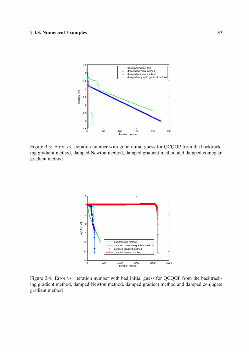
3.3 Error vs. iteration number with good initial guess for QCQOP from the back-tracking gradient method, damped Newton method, damped gradient methodand damped conjugate gradient method . . . . . . . . . . . . . . . . . . . . . . 37
3.4 Error vs. iteration number with bad initial guess for QCQOP from the back-tracking gradient method, damped Newton method, damped gradient methodand damped conjugate gradient method . . . . . . . . . . . . . . . . . . . . . . 37
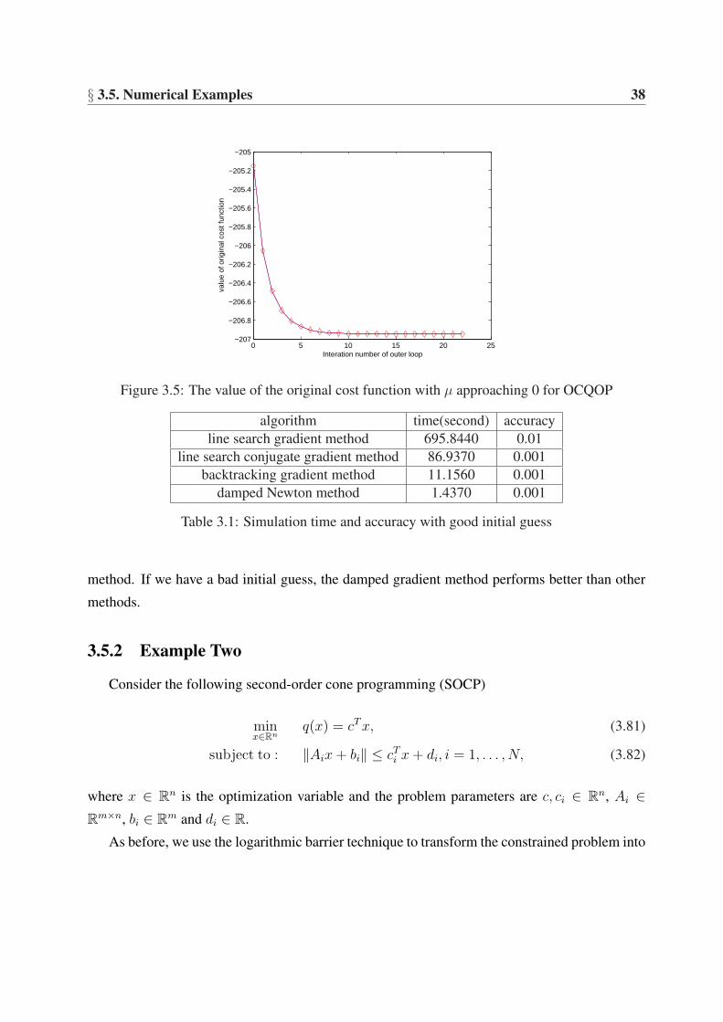
3.5 The value of the original cost function with µ approaching 0 for OCQOP . . . . . 383.6 Error vs. iteration number for SOCP from the damped Newton method, damped
gradient method and damped conjugate gradient method . . . . . . . . . . . . . 413.7 The value of the original cost function with µ approaching 0 for SOCP . . . . . . 42
4.1 The tangent and normal spaces . . . . . . . . . . . . . . . . . . . . . . . . . . . 464.2 Move a tangent vector parallel to itself to another point on the manifold . . . . . 474.3 Parallel transport (infinitesimal space) . . . . . . . . . . . . . . . . . . . . . . . 47
5.1 Conjugate gradient direction on Riemannian Manifolds . . . . . . . . . . . . . . 70
6.1 The result of damped Newton method for the self-concordant function definedon the circle . . . . . . . . . . . . . . . . . . . . . . . . . . . . . . . . . . . . . 85
6.2 The result of damped Newton method for the self-concordant function definedon high-dimension sphere . . . . . . . . . . . . . . . . . . . . . . . . . . . . . . 86
6.3 The result of damped conjugate gradient method for the self-concordant functiondefined on high-dimension sphere . . . . . . . . . . . . . . . . . . . . . . . . . 87
6.4 The result of the the damped Newton method for the self-concordant functiondefined on the Hyperboloid model . . . . . . . . . . . . . . . . . . . . . . . . . 100
ix
6.5 The result of the damped conjugate gradient method for the self-concordant func-tion defined on the Hyperboloid model . . . . . . . . . . . . . . . . . . . . . . . 101
7.1 The result of Quasi-Newton Method compared against the Newton method andsteepest decent method . . . . . . . . . . . . . . . . . . . . . . . . . . . . . . . 115
x

List of Notation
R The real numbers.Rn The set of all real n× 1 vectors.Rn×p The set of all real n× p matrices.AT The transpose of a matrix A.In The n× n identity matrix.det(A) The determinant of matrix A.diag(x) The n× n diagonal matrix for x ∈ Rn whose ith diagonal term is xi.vec(A) The column vector consisting of the stacked columns of the matrix A.tr(A) The sum of the diagonal elements of a matrix A.‖x‖ The Euclidean norm of a vector x ∈ Rn, ‖x‖ =
√xT x.
‖A‖F The Frobenius Norm of a matrix A ∈ Rn×p, ‖A‖F =√
tr(AT A).TpM The tangent space of a manifold M at p ∈ M .〈X,Y 〉p The inner product defined on X, Y ∈ TpM , where p ∈ M and M is a
Riemannian manifold.‖X‖p The norm of a tangent vector X ∈ TpM , ‖X‖p =
√〈X, X〉p, wherep ∈ M and M is a Riemannian manifold.
ExpptX The geodesic emanating from p ∈ M in the direction X ∈ TpM where M
is a Riemannian manifold.τpq The parallel transport from TpM to TqM along the given geodesic
connecting p and q where p, q ∈ M and M is a Riemannian manifold.Sn The n−dimensional unit sphere in Rn+1, Sn = x ∈ Rn+1|xT x = 1.In The n−dimensional hyperboloid model in Rn+1,
In = x ∈ Rn+1| −∑ni=1 x2
i + x2n+1 = 1, xn+1 > 0.
St(n, p) The Stiefel manifold defined by the set of real n× p orthogonal matrices,St(n, p) := X ∈ Rn×p|XT X = Ip.
Gr(n, p) The Grassmann manifold defined by the set of all p−dimensional spaces ofRn.
xi

Chapter 1
Introduction
1.1 Overview
Optimization plays an important role in both research and applications. The essence of op-
timization problems is to search the minimum or maximum of cost functions. Methods to solve
optimization problems have been widely studied. For example, given a cost function f defined
on the whole Rn, one can use conventional methods such as the steepest descent method, con-
jugate gradient method or Newton method to minimize this function. However, in engineering,
many cost functions are subject to constraints. For example, see [53, 72]. Minimizing functions
subject to inequality constraints have resulted in new optimization methods. If a constraint is
linear or nonlinear convex, the interior point method is commonly used. Assuming that we have
an optimization problem defined on a linear or nonlinear convex constraint, the idea of the in-
terior point method is to transform the constrained optimization problem into a parameterized
unconstrained one using a barrier penalty function, commonly constructed by a self-concordant
function defined by Nesterov and Nemirovskii [58]. The barrier function remains relatively flat
in the interior of the constraint while tending to infinity when approaching the boundary. A new
cost function including the original cost function and the barrier function is constructed. Then
we can use plain methods to minimize the new cost function until we find the optimal value of
the original problem.
In recent years, optimization on smooth manifolds has drawn more attention since it can re-
duce the dimension of optimization problems compared to solving the original problem in their
ambient Euclidean space. Its applications appear in medicine [3], signal processing [53], ma-
chine learning [60], computer vision [50, 32], and robotics [35, 33]. Optimization approaches
1
§ 1.2. Literature Review 2
on smooth manifolds can be categorized into Riemannian approaches and non-Riemannian ap-
proaches.
1. Methods of solving minimization problems on Riemannian manifolds have been exten-
sively researched. For more details, see [70, 67, 18, 19, 71]. In fact, traditional optimiza-
tion methods such as the steepest gradient method, conjugate gradient method and Newton
method in Euclidean space can be applied to optimization on Riemannian manifolds with
slight changes. A typical intrinsic approach for minimization is based on the computation
of geodesics and covariant differentials, which may be resource expensive. However, there
are many meaningful cases where the computation can be very simple. An example is the
hyperboloid space, where the geodesic and parallel transformation can be computed via
hyperbolic functions and vector calculations. Another simple but non-trivial case is the
sphere, where the geodesic and parallel transformation can be computed via trigonometri-
cal functions and vector calculation. As a consequence, it is natural to ask: can we define
self-concordant functions on Riemannian manifolds and what is the related interior point
method? Clearly solving such a question will have practical importance and theoretical
completeness.
2. As mentioned above, the computational cost of computing geodesics is often relatively
high. For this and other reasons, Manton [53] developed a more general framework for
optimization on manifolds. This framework does not require a Riemannian structure to be
defined on the manifold and its greater generality allows more efficient algorithms to be
developed.
In the rest of this chapter, we first review the developments in the interior point methods,
self-concordant functions and the optimization on smooth manifolds. Then the motivation and
research aims are given. Finally, the outline of this thesis is presented.
1.2 Literature Review
1.2.1 Interior Point Method and Self-concordant Functions
The basic idea of interior-point methods is as follows. If f(x) is a linear convex cost function
we wish to minimize on a convex set Q of Rn, and if g(x) is a barrier function meaning that g(x)

§ 1.2. Literature Review 3
approaches infinity on the boundary of Q, then we solve the sequence of optimization problems
xk = arg minx
1
µk
f(x) + g(x) where µk → 0 and µk > 0. As µk converges to zero, xk will
converge to the minimal point of the original cost function f(x) constrained to Q, under the
assumption that f(x) and g(x) are convex.
The history of the interior point method can be traced back to Khachiyan’s work [45] which
first introduced the polynomial-time interior point method in 1979. However, the start of the
interior-point revolution was Karmarkar’s claim in 1984 of a polynomial-time linear program-
ming method [43]. Then the equivalence between Karmarkar’s method and the classical loga-
rithmic barrier method was shown in 1986 [26].
The milestone work of Nesterov and Nemirovskii [58] presented a new special class of bar-
rier methods and developed polynomial-time complexity results for new convex optimization
problems. Their proposed self-concordant functions are critically important in powerful interior
point polynomial algorithms for convex programming in Euclidean space. The significance of
these functions lies in two aspects. Firstly, they provide many of logarithmic barrier functions
which are important in interior point methods for solving convex optimization problems. Sec-
ondly, the proposed damped Newton method for optimizing self-concordant functions does not
involve unknown parameters. This is useful for constrained optimization problems. It is also
worth noting that using self-concordant barrier functions guarantees the original problem to be
solved in a polynomial time for a pre-defined precision.
1.2.2 Optimization On Smooth Manifolds
As stated before, traditional optimization techniques in Euclidean space can have their coun-
terparts on smooth manifolds, which have been studied. In this section, we first review the
classical Riemannian approaches and then the relatively recent non-Riemannian approaches.
Riemannian Approach
1. Steepest descent method on manifolds
The steepest descent method is the simplest method for the optimization on Riemannian
manifolds and it has good convergence properties but slow linear convergence rate. This
method was first introduced to manifolds by Luenberger [48, 49] and Gabay [25]. In the
early nineties, this method was carried out to problems in systems and control theory by
Brockett [13], Helmke and Moore [34], Smith [66] and Mahony [51].

§ 1.2. Literature Review 4
2. Newton method on manifolds
Compared against the steepest descent method, the Newton method has a faster (quadratic)
local convergence rate. In 1982, Gabay extended the Newton method to a Riemannian
sub-manifold of Rn by updating iterations along a geodesic. Other independent work has
been developed to extend the Newton method on Riemannian manifolds by Smith [67] and
Mahony [51, 52] restricting to the compact Lie group, and by Udriste [70] restricting to
convex optimization problems on Riemannian manifolds. Edelman, Arias and Smith [19]
also introduced a Newton method for the optimization on orthogonality constraints - the
Stiefel and Grassmann manifolds. There is also a recent paper by Dedieu, Priouret and
Malajovich [18] which studied the Newton method to find zero of a vector field on general
Riemannian manifolds.
3. Quasi-Newton method on manifolds
Even though the Newton’s method has faster quadratic convergence rate, it requires com-
puting the inverse of a symmetric matrix, called the Hessian consisting of the second order
local information of the cost function. Therefore, it increases the computational cost. In
order to avoid this problem, the quasi-Newton method in Euclidean space was presented
by Davidon [17] in late 1950s. This method uses only the first order information of the
cost function to approximate the Hessian inverse and has a super-linear local convergence
rate. Since then, various quasi-Newton methods have been introduced. However, among
them, the most popular methods are the Davidon-Fletcher-Powell (DFP) [22] method and
the Broyden [15, 16] Fletcher [21] Goldfarb [28] Shanno [65] (BFGS) method.
In the early eighties, Gabay [65] firstly generalized the BFGS method to a Riemannian
manifold. However, he did not give the complete proof of the convergence of his method.
Recently, Brace and Manton [12] developed an improved BFGS method on the Grassmann
manifold and achieved a lower computational complexity compared to Gabay’s method.
4. Conjugate gradient method on manifolds
While considering the large scale optimization problems with sparse Hessian matrices,
the quasi-Newton methods encounters difficulties. Due to avoiding computing the inverse
of the Hessian, the conjugate gradient method can be used for solving such problems.
This method was originally developed by Hestenes and Stiefel [38] in the 1950s to solve
large scale systems of linear equations. Then in the mid 1960s, Fletcher and Reeves [24]

§ 1.2. Literature Review 5
popularized this method to solve unconstrained optimization problems. In 1994, Smith
[67] extended this method to Riemannian manifolds and later Edelman, Arias and Smith
[19] applied his method specifically on the Stiefel and Grassmann manifolds.
Non-Riemannian Approach
The traditional methods for optimizing a cost function on a manifold all start by endowing
the manifold with a metric structure, thus making it into a Riemannian manifold. The reason for
doing so is that it allows Euclidean algorithms, such as steepest descent and Newton methods, to
be generalised reasonably straightforwardly; the gradient is replaced by the Riemannian gradient,
for example. However, as pointed out in [54], the introduction of a metric structure is extraneous
to the underlying optimisation problem and thus, in general, is detrimental. (A possible exception
is when the cost function is somehow related to the Riemannian geometry, such as if it is defined
in terms of the distance function on the Riemannian manifold.)
For an arbitrary smooth manifold, the only structure we know is that around any point, the
manifold looks like Rn. This is explained as follows. Let M be a smooth n-dimensional mani-
fold. For every point p ∈ M , there exists a smooth map
ψp Rn → M, ψp(0) = p (1.1)
which is a local diffeomorphism around 0 ∈ Rn. Such a ψp is called a local parametrization.
In [53], Manton gave a general framework for developing numerical algorithms for minimis-
ing a cost function defined on a manifold. The framework entailed choosing a particular local
parametrization about each point on the manifold. In the same paper, this framework was ap-
plied to the Stiefel and Grassmann manifolds, and as an example, the local parametrizations were
chosen, in a certain sense, to be projections from the tangent space to the manifold itself. Based
on this parametrization, the corresponding steepest descent and Newton methods were shown to
reduce the computational complexity compared with the traditional Riemannian methods.

§ 1.3. Motivation and Research Aims 6
1.3 Motivation and Research Aims
1.3.1 Motivation
Since from the optimization point of view self-concordant functions enjoy good tractabil-
ity, it is tempting to extend its definition to manifolds and develop corresponding optimization
algorithms. In [57], Nesterov only provided a Newton-based algorithm for optimization of a self-
concordant function in Euclidean space. Although this algorithm has quadratic convergence, the
requirement of computing the inverse of the Hessian matrix creates significant computational
complexity per iteration. To avoid this problem, some gradient-based methods such as gradient
and conjugate gradient methods can be taken first before switching to Newton-based methods.
Due to the importance of gradient-based method, we are motivated to develop a damped gradient
method and a damped conjugate gradient method for optimization of self-concordant functions.
Furthermore, it is expected that these two methods can be applied to the optimization of self-
concordant functions on Riemannian manifolds. Consequently, they can provide guidance to
develop interior point methods on Riemannian manifolds.
In addition, although the steepest and Newton methods have been developed as the non-
Riemannian approach, to our best knowledge, we are not aware of any published papers intro-
ducing the non-Riemannian based quasi-Newton methods on smooth manifolds. Since the quasi-
Newton method has prominent advantages, we are also motivated to develop a quasi-Newton
method on smooth manifolds.
1.3.2 Research Aims
The aims of this thesis are to
• fully explore properties of the self-concordant function in Euclidean space and develop
gradient-based algorithms for optimization of such function;
• define the self-concordant function on Riemannian manifolds, explore its properties and
devise corresponding optimization algorithms;
• generalize a quasi-Newton method on smooth manifolds without the Riemannian stucture.

§ 1.4. Outline of This Thesis 7
1.4 Outline of This Thesis
To achieve our research aims, besides this introduction chapter, this thesis consists of three
parts.
1.4.1 Self-concordant Functions in Euclidean Space
Part I includes three chapters and mainly focuses on the properties of self-concordant func-
tions in Euclidean space and algorithms for the optimization of such functions.
In Chapter 2, we review the definition of self-concordant functions in Euclidean space, in-
troduced by Nesterov and Nemirovskii in [58] and their properties. We also recall the damped
Newton algorithm from [58] for the optimization of self-concordant functions and its conver-
gence properties.
In Chapter 3, we propose a damped gradient method and a damped conjugate gradient method
for optimization of self-concordant functions. A damped Newton method introduced by Nes-
terov is an ordinary Newton method but with a step-size selection rule chosen to guarantee con-
vergence. Based on the gradient and conjugate gradient methods, our methods provide novel
step-size selection rules which are proved to ensure that algorithms converge to the global mini-
mum. The advantage of our methods over the damped Newton method is that the former have a
lower computational complexity. Then, we build up an interior point method based on our pro-
posed damped conjugate gradient method. Finally, our algorithms are applied to second order
cone programming and quadratically constrained quadratic optimization problems.
1.4.2 Self-concordant Functions On Riemannian Manifolds
Part II includes three chapters and mainly focuses on the properties of self-concordant func-
tions on Riemannian manifolds and algorithms for the optimization of such functions.
In chapter 4, the self-concordant functions are defined on Riemannian manifolds. Then gen-
eralizations of the properties of self-concordant functions on Riemannian manifolds are derived.
Based on properties, a damped Newton algorithm is proposed for optimization of self-concordant
functions, which guarantees that the solution falls in any given small neighborhood of the opti-
mal solution, with its existence and uniqueness also proved in this chapter, in a finite number of
steps. It also ensures quadratic convergence within a neighborhood of the minimal point.

§ 1.4. Outline of This Thesis 8
In Chapter 5, we present a damped conjugate gradient method for optimization of self-
concordant functions defined on smooth Riemannian manifolds. A damped conjugate gradient
method is an ordinary conjugate gradient method with an explicit step-size selection rule. It is
proved that this method guarantees to converge to the global minimum super-linearly. Com-
pared against the damped Newton method, the damped conjugate gradient method has a lower
computational complexity.
In Chapter 6, we introduce three examples in which the cost functions are self-concordant
on different Riemannian manifolds. We also applied our damped Newton method and conjugate
gradient method into minimizing these three cost functions. Simulation results show the nice
performance of our algorithms.
1.4.3 The Quasi-Newton Methods
Part III includes one chapter and mainly focuses developing a new quasi-Newton method on
smooth manifolds.
In Chapter 7, we propose a new quasi-Newton method on smooth manifolds based on the
local parametrization. This method is proved to converge to the minimum of the cost function. To
demonstrate its efficiency, we applied this quasi-Newton method into a cost function defined on
the Grassmann manifold. The simulation result shows our method has super-linear convergence.

Part I
Self-concordant Functions in EuclideanSpace
9

Chapter 2
Introduction to Self-Concordant Functionsin Euclidean Space
2.1 Introduction
In this chapter, we review the self-concordant function in Euclidean space, which is proposed
by Nesterov and Nemirovskii in [58]. A damped Newton method was also presented in [58] for
optimization of such function. In this chapter, we briefly introduce the damped Newton method
and its convergence properties. For more details, refer to [58] and [57].
2.2 Definition and Properties
In this section, we recall some concepts and properties related to self-concordant functions
defined in Euclidean space.
Throughout this chapter, f will denote a real-valued function from a convex subset Q of Rn.
We consider constrained optimization problems of the following form
minx∈Q
f(x) f : Q ⊂ Rn → R. (2.1)
In general, it is hard to solve (2.1), even numerically. However, if f has certain nice proper-
ties, there exist powerful techniques to solve (2.1). In [57], Nesterov considered the case when f
is self-concordant, defined as follows.
10

§ 2.2. Definition and Properties 11
Definition 1. Let f : Q → R be a C3-smooth closed convex function defined on an open domain
Q ⊂ Rn. Then f is self-concordant if there exists a constant Mf > 0 such that the inequality
|D3f(x)[u, u, u]| ≤ MfD2f(x)[u, u]3/2 (2.2)
holds for any x ∈ Q and direction u ∈ Rn.
Recall that f being C3-smooth means f is three-times continuously differentiable. A convex
function f : Q → R is called closed if its epigraph, defined as epi(f) = (x, t) ∈ Q × R|t ≥f(x), is closed. The reason why f is required to be closed in Definition 1 is to ensure that f
behaves nicely on the boundary of its domain; see (2.8). Also, the second and third directional
derivatives D2 and D3 are defined as follows. Given x ∈ Q and u ∈ Rn,
D2f(x)[u, u] =d2
dt2
t=0
f(x + tu), (2.3)
D3f(x)[u, u, u] =d3
dt3
t=0
f(x + tu). (2.4)
We consider the special case of the optimization problem in (2.1) where f satisfies the fol-
lowing assumption.
Assumption 1. The function f in (2.1) is self-concordant, has a minimum in Q and for all x ∈ Q,
f ′′(x) is nonsingular. By scaling f if necessary, it is assumed without loss of generality that f
satisfies (2.2) with Mf = 2.
The need for assuming f has a minimum in Assumption 1 can be seen from the example
g(x) = − ln x defined on (0, +∞) where g is self-concordant but g has no minimum. If f has a
minimum, then it is unique because f is strictly convex by Assumption 1. Note that by Theorem
4.1.3 in [57], f ′′(x) is nonsingular for all x ∈ Q if the domain Q contains no straight line.
Functions satisfying Assumption 1 have interesting properties which facilitate our further
analysis. For details, see [57]. For a given x ∈ Q, we introduce a local norm on Rn
‖u‖x = 〈f ′′(x)u, u〉 12 , u ∈ Rn (2.5)
and the Dikin ellipsoid of unit length
W 0(x) = y ∈ Rn∣∣‖y − x‖x < 1. (2.6)
§ 2.2. Definition and Properties 12
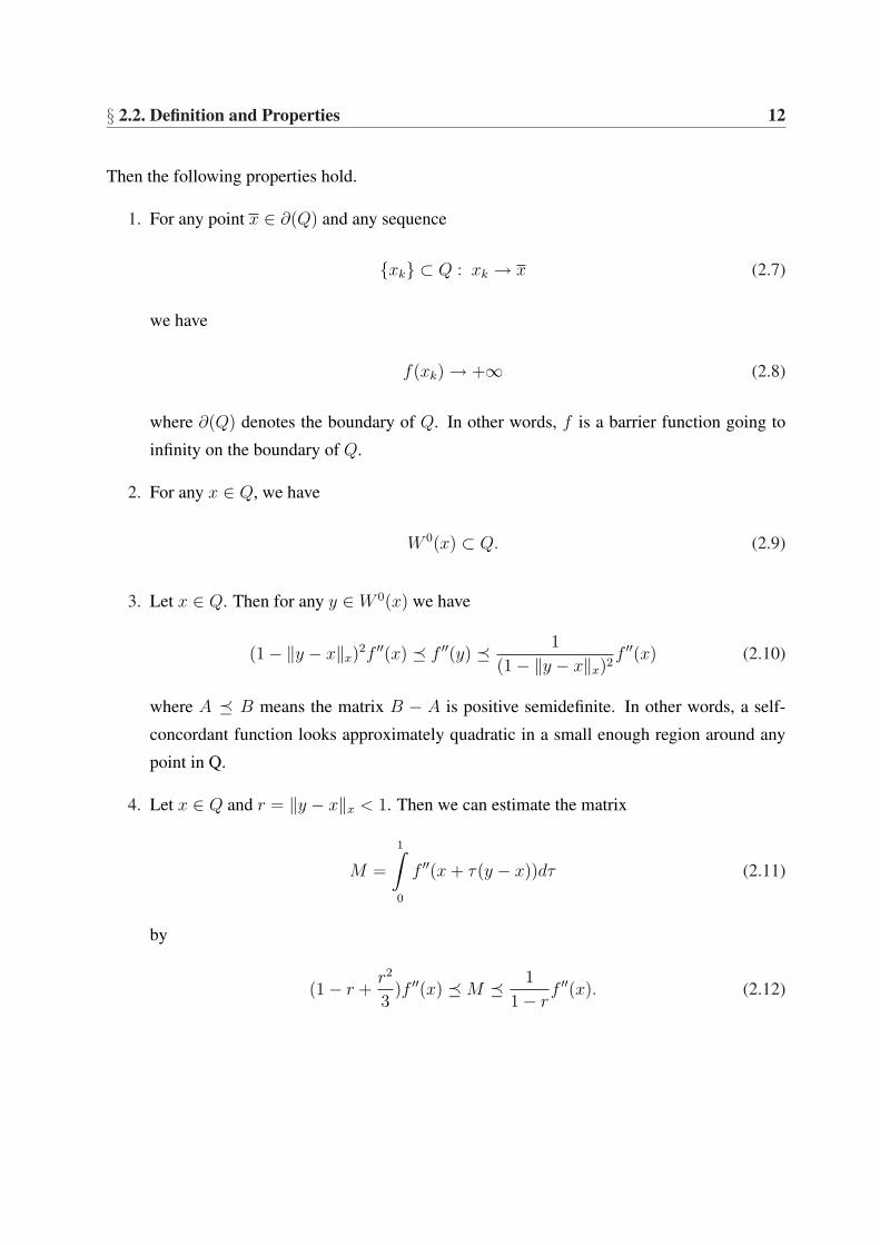
Then the following properties hold.
1. For any point x ∈ ∂(Q) and any sequence
xk ⊂ Q : xk → x (2.7)
we have
f(xk) → +∞ (2.8)
where ∂(Q) denotes the boundary of Q. In other words, f is a barrier function going to
infinity on the boundary of Q.
2. For any x ∈ Q, we have
W 0(x) ⊂ Q. (2.9)
3. Let x ∈ Q. Then for any y ∈ W 0(x) we have
(1− ‖y − x‖x)2f ′′(x) ¹ f ′′(y) ¹ 1
(1− ‖y − x‖x)2f ′′(x) (2.10)
where A ¹ B means the matrix B − A is positive semidefinite. In other words, a self-
concordant function looks approximately quadratic in a small enough region around any
point in Q.
4. Let x ∈ Q and r = ‖y − x‖x < 1. Then we can estimate the matrix
M =
1∫
0
f ′′(x + τ(y − x))dτ (2.11)
by
(1− r +r2
3)f ′′(x) ¹ M ¹ 1
1− rf ′′(x). (2.12)

§ 2.3. Damped Newton Algorithm 13
5. For any x, y ∈ Q we have
f(y) ≥ f(x) + 〈∇f(x), y − x〉+ ω(‖y − x‖x) (2.13)
where ω(t) = t− ln(1 + t). Note that if y 6= x, then ω(‖y − x‖x) is positive, hence (2.13)
gives a useful lower bound on f(y).
6. Let x ∈ Q and ‖y − x‖x < 1. Then
f(y) ≤ f(x) + 〈∇f(x), y − x〉+ ω∗(‖y − x‖x) (2.14)
where ω∗(t) = −t − ln(1 − t). Similar to above, if y 6= x, then ω∗(‖y − x‖x) is also
positive, and hence (2.14) gives a useful upper bound on f(y).
Lemma 1. Let f : Q → R be a C3-smooth closed convex function defined on an open domain
Q ⊂ Rn. Then f is self-concordant if and only if there exists a constant Mf > 0 such that for all
x ∈ Q and any directions u1, u2, u3 ∈ Rn, we have
|D3f(x)[u1, u2, u3]| ≤ Mf
3∏i=1
‖ui‖x.
Lemma 1 gives an alternative definition of a self-concordant function.
2.3 Damped Newton Algorithm
In this section, we review the damped Newton algorithm [57] for optimization of self-concordant
functions. This algorithm is a Newton-based method but with an explicit step-size rule.
To illustrate the algorithm, the Newton decrement λ(x) is introduced, defined in terms of the
gradient and the Hessian as follows
λ(x) = 〈[f ′′(x)]−1∇f(x),∇f(x)〉 12 . (2.15)
The Newton decrement λ(x) plays an important role in the optimization of self-concordant func-
tions based on the Newton method.
Nesterov constructed a damped Newton method as follows to minimize f in (2.1) when f
satisfies Assumption 1.

§ 2.3. Damped Newton Algorithm 14
Algorithm 1. (Damped Newton Algorithm) [57]
step 0: Select an initial point x0 ∈ Q and set k=0;
step k: Set
λ(xk) = 〈[f ′′(xk)]−1∇f(xk),∇f(xk)〉 1
2
xk+1 = xk − 1
1 + λ(xk)[f ′′(xk)]
−1∇f(xk).
Increment k and repeat until convergence.
It is worth noting that Algorithm 1 guarantees in every step that xk+1 lies in the Dikin ellipsoid
around xk. In other words, the sequence xk given by Algorithm 1 lies in the domain Q.
The following proposition shows that the damped Newton method decreases the value of f(x)
significantly.
Proposition 2.3.1. [57] Let xk be a sequence generated by Algorithm 1, where the cost func-
tion f : Q → R in 2.1 satisfies Assumption 1. Then, ∀k, we have
f(xk+1) ≤ f(xk)− ω(λ(xk)) (2.16)
where ω(t) = t− ln(1 + t).
The following proposition illustrates that the local convergence of Algorithm 1 is quadratic.
Proposition 2.3.2. [57] Let xk be a sequence generated by Algorithm 1, where the cost func-
tion f : Q → R in (2.1) satisfies Assumption 1. Then ∀k
λ(xk+1) ≤ 2λ2(xk). (2.17)

Chapter 3
Damped Gradient and Conjugate GradientMethods
3.1 Introduction
Background In [57], Nesterov developed a damped Newton method to compute the mini-
mum of a self-concordant function. The key feature of this method is that it provides an explicit
step-size choice based on the Newton method and the value of the function strictly decreases in
each iteration of this method. In addition, this method guarantees that the iteration sequence re-
mains in the domain of the cost function. It was proved that this method always converges to the
minimum of the self-concordant function. On the other hand, since the damped Newton method
is Newton-based, it possesses certain inherent disadvantages of the Newton method. One of them
is the expensive computational cost involved in computing the inverse of the Hessian matrix of
the cost function. Therefore, we are motivated to build up gradient-based methods with explicit
step-size rules for the optimization of self-concordant functions.
Concerning finding an appropriate step-size, several rules have been developed for gradient-
based methods. For instance, the gradient-based step-size can be determined via various line
search methods for constrained optimization problems. However, the resulting disadvantage of
these methods is that they may increase the cost of additional iterations for a suitable step-size.
In [68], Sun and Zhang presented an explicit formula for step-size selection to find the minimum
of an unconstrained function based on the conjugate gradient direction. This method is shown
to ensure convergence to the local minimum. However, it does not generalize immediately to
the constrained case since it can not guarantee that the iterations remain inside the constrained
15

§ 3.1. Introduction 16
domain.
Our work In this chapter, we present a damped gradient method and a damped conjugate
gradient method to minimize self-concordant functions on Euclidean space. Our methods are
shown to converge to the optimal solution of a self-concordant function if it exists. One of
the advantages of our methods is that they only consist of computing the gradient and Hessian
matrix of the cost function without computing the inverse of the Hessian matrix. In every step,
the complexity of these two methods is O(n2) instead of O(n3) in the damped Newton method,
where n is the dimension of the variable.
Chapter outline The rest of this chapter is organized as follows. We review the traditional
gradient and conjugate gradient methods in Section 3.2. In Section 3.3, the damped gradient and
conjugate gradient methods are derived and it is shown that these two algorithms converge to the
minimum of the cost function provided the cost function is self-concordant. In the last section,
two examples are included to illustrate the convergence properties of these algorithms.
Notation: The symbol Sn denotes the set of n dimensional real symmetric matrices. An inner
product on Sn is:
〈X, Y 〉F = trace(XY ). (3.1)
It induces the Frobenius norm ‖X‖F = 〈X, X〉12F . The notation 0 ¹ X means that X is positive
semidefinite. For any X, Y ∈ Sn, Y ¹ X means that X−Y is positive semidefinite. Throughout,
the Euclidean inner product on Rn is used, namely 〈x, y〉 = xT y. It induces the Euclidean norm
‖x‖ = 〈x, x〉 12 . The symbol ∂(Q) denotes the boundary of the set Q. Throughout, f will denote
a real-valued function defined on a convex subset Q ofRn. We consider constrained optimization
problems of the form
minx∈Q
f(x), f : Q ⊂ Rn → R. (3.2)

§ 3.2. Review of The Gradient and Conjugate Gradient Methods 17
3.2 Review of The Gradient and Conjugate Gradient Meth-
ods
In this section, we review descent methods such as the gradient method and the conjugate
gradient method for solving the unconstrained optimization problem
minx∈Rn
f(x), f : Rn → R. (3.3)
Motivation for introducing our novel damped methods in Section 4 for optimization of self-
concordant functions is also given.
Descent algorithms for solving (3.3), such as the gradient and conjugate gradient methods,
are of the following form. Initially, a point x0 ∈ Rn is chosen at random. Then the sequence xkis generated according to the rule xk+1 = xk + hkHk where Hk is called the descent direction
and hk the step-size. There are several step-size rules commonly used:
1. The sequence hk∞k=0 is chosen in advance [57]. Two examples are a constant step-size
hk = h > 0, or hk = h√k+1
, h > 0.
2. Line search [57]: hk = arg minh≥0
f(xk + hHk).
3. Backtracking [72]: Start with unit step-size hk = 1, then reduce it by the multiplicative
factor β until the stopping condition f(xk +hkHk) ≤ f(xk)+αhk〈f ′(xk), Hk〉 holds. The
parameter α is typically chosen between 0.01 and 0.3, and β between 0.1 and 0.8.
Although these step-sizes can work well in practice, they each have their limitations. The
first rule cannot guarantee that the decent algorithm converges to the solution of (3.3). Indeed,
the values f(xk) need not even form a decreasing sequence. In general the second rule is only
acceptable in theory because the line search is often too hard to compute in practice. The choice
of α and β in the third rule is somewhat arbitrary.
Different algorithms use different rules for determining the descent direction Hk, as now
reviewed.
The gradient method chooses Hk to be−f ′(xk). Since it requires only first order information,
the gradient method is relatively cheap to implement. Often, a few steps of the gradient method
are taken before switching to a higher order method.

§ 3.2. Review of The Gradient and Conjugate Gradient Methods 18
xk
xk+1
Hk
Hk+1
f(xk+1)
Figure 3.1: Conjugate gradient in Euclidean space
The conjugate gradient method is a popular method because it is easy to implement, has low
storage requirements, and provides superlinear convergence in the limit. The primary idea of the
conjugate gradient method is to use the conjugacy to find the search direction.
Algorithm 2. (Conjugate gradient algorithm)step 0: Select an initial point x0, compute H0 = −f ′(x0), and set k = 0.
step k: If f ′(xk) = 0 then terminate. Otherwise, compute hk with the exact line search
method.
Set xk+1 = xk + hkHk.
Set
γk+1 = −‖f′(xk+1)‖2
〈f ′(xk), Hk〉 , (3.4)
Hk+1 = −f ′(xk+1) + γk+1Hk. (3.5)

§ 3.3. The Damped Method 19
If k + 1 mod n ≡ 0, set Hk+1 = −f ′(xk+1). Increment k and repeat until convergence.
Figure 3.1 illustrates the conjugate gradient direction in Euclidean space. Whereas Hk+1
in the gradient method depends only on f ′(xk+1), in the conjugate gradient method, Hk+1 relies
also on the past history of Hk via a weighting factor γk+1. In (3.4), γk+1 is given by the conjugate
descent method in [23]; other choices are possible.
Consider applying a gradient or conjugate gradient method to the constrained optimization
problem (3.2). None of the three step-size rules presented earlier are suitable; the first and third
rules cannot ensure xk remains in Q, while the second rule is difficult to implement in practice.
This motivates the introduction of novel step-size rules which guarantee the convergence of the
algorithm to the minimum of the cost function.
3.3 The Damped Method
In this section, we derive explicit step-size rules for use in gradient and conjugate gradient
methods for solving (3.2) when f is self-concordant. These step-size rules guarantee convergence
to the global minimum.
3.3.1 The Damped Gradient Method
Let f in (3.2) satisfy Assumption 1. Suppose we have a point xk in Q at time k. Given an
appropriate step-size hk, the gradient method sets xk+1 = xk−hkf′(xk). We propose choosing hk
to maximize the bound in (2.14). Later, in Theorem 3.3.1, it is proved such a strategy guarantees
convergence to the minimum of f .
From (2.14), provided xk+1 ∈ W (xk) and hk ≥ 0, we have
f(xk)− f(xk+1) ≥ hk‖f ′(xk)‖2 + hk‖f ′(xk)‖xk
+ ln(1− hk‖f ′(xk)‖xk). (3.6)
The right hand side is of the form ψ(hk) where ψ(h) = αh+ln(1−βh) with α = ‖f ′(xk)‖2+
‖f ′(xk)‖xkand β = ‖f ′(xk)‖xk
. Since h is a descent step, it is required to be positive. Moreover,
if we are not at the minimum of f , then β will be strictly positive. Therefore, ψ is defined on
the interval [0, 1/β). Note that if hk ∈ [0, 1/β), then xk+1 ∈ W (xk) as required for (3.6) to be a
valid bound.

§ 3.3. The Damped Method 20
Differentiating ψ(h) yields
ψ′(h) = α− β
1− βh, (3.7)
ψ′′(h) = − β2
(1− βh)2< 0, (3.8)
showing that ψ(h) is concave on its domain [0, 1/β). It achieves its maximum at
h =α− β
αβ. (3.9)
Let λ(x) = ‖f ′(x)‖2‖f ′(x)‖x
. Substituting α and β into (3.9), we obtain the rule
hk =λk
(1 + λk)‖f ′(xk)‖xk
(3.10)
where λk = λ(xk) = ‖f ′(xk)‖2‖f ′(xk)‖xk
.
This motivates us to define the following damped gradient method.
Algorithm 3. (Damped Gradient Algorithm)step 0: Select an initial point x0 ∈ Q and set k = 0.
step k: If f ′(xk) = 0 then terminate. Otherwise, set
λk =‖f ′(xk)‖2
‖f ′(xk)‖xk
,
hk =λk
(1 + λk)‖f ′(xk)‖xk
,
xk+1 = xk − hkf′(xk).
Increment k and repeat until convergence.
The convergence of Algorithm 3 is proved in Theorem 3.3.1 with the help of Lemma 2.
Lemma 2. Let xk be a sequence generated by Algorithm 3, where the cost function f : Q → R
in (3.2) satisfies Assumption 1 in Chapter 1. Then:
1. ∀k, xk ∈ Q.

§ 3.3. The Damped Method 21
2. If f ′(xk) 6= 0, then f(xk+1) ≤ f(xk)− ω(λk) < f(xk), where ω(t) = t− ln(1 + t).
3. Let x∗ ∈ Q be the solution of (3.2). If x ∈ Q satisfies x 6= x∗, then λ(x) > 0. Moreover,
limx→x∗
λ(x) = 0.
Proof:
1. From the earlier derivation, it was already proved that
xk+1 ∈ W (xk). (3.11)
Therefore, from (2.9) and the fact that x0 ∈ Q, it follows that xk ∈ Q.
2. Substituting hk into (3.6), we obtain
f(xk+1) ≤ f(xk)− ω(λk) (3.12)
where ω(t) = t− ln(1 + t). Since f ′(xk) 6= 0 implies λk > 0 and, from (2.13), w(t) > 0
for t > 0, the result follows.
3. Recall that Assumption 1 implies x∗ is unique. Therefore f ′(x) = 0 only and only if
x = x∗. Suppose x ∈ Q but x 6= x∗. Since f ′′(x) is positive definite by Assumption 1 and
f ′(x) 6= 0 we have λ(x) > 0.
Let K = x∣∣‖x − x∗‖ ≤ ρ where ρ > 0 is sufficiently small such that K ⊂ Q. Let
νmin(f ′′(x)) denote the minimum eigenvalue of the Hessian matrix f ′′(x). Then θ =
minx∈K
νmin(f ′′(x)) exists since K is compact and νmin(f ′′(x)) is continuous. Since f ′′(x) is
positive definite on Q by Assumption 1, θ > 0. Moreover, for any x ∈ K and any direction
u ∈ Rn, we have
uT f ′′(x)u = ‖u‖2x ≥ θ‖u‖2. (3.13)
Therefore, for x ∈ K, we obtain
λ(x) =‖f ′(x)‖2
‖f ′(x)‖x
≤ 1√θ‖f ′(x)‖. (3.14)

§ 3.3. The Damped Method 22
Therefore, at x∗, we get
0 ≤ limx→x∗
λ(x) ≤ limx→x∗
1√θ‖f ′(x)‖. (3.15)
Since f ′(x) is continuous and f ′(x∗) = 0, limx→x∗
λ(x) = 0.
¤
Theorem 3.3.1. Consider the constrained optimization problem in (3.2). If the cost function
f : Q → R in (3.2) satisfies Assumption 1 in Chapter 1, then Algorithm 3 converges to the
unique minimum of f .
Proof: Let K = y∣∣f(y) ≤ f(x0) where x0 denotes the initial point. Let x∗ be the solution
of (3.2). Then for any y ∈ K in view of (2.13), we have
f(y) ≥ f(x∗) + ω(‖y − x∗‖x∗). (3.16)
It follows from (3.46) that
ω(‖y − x∗‖x∗) ≤ f(y)− f(x∗) ≤ f(x0)− f(x∗); (3.17)
Note that ω(t) is strictly increasing in t. Therefore, ‖y − x∗‖x∗ ≤ t where t is the unique
positive root of the following equation
ω(t) = f(x0)− f(x∗). (3.18)
Thus, K is closed bounded and hence compact.
From Lemma 2, we have
f(xk+1) ≤ f(xk)− ω(λk). (3.19)
Summing up the inequalities (3.19) for k = 0 . . . N , we obtain
N∑
k=0
ω(λk) ≤ f(x0)− f(xN+1) ≤ f(x0)− f(x∗), (3.20)

§ 3.3. The Damped Method 23
where x∗ is the solution of (3.2). As a consequence of (3.20), we have
ω(λk) → 0 as k →∞ (3.21)
and therefore
λk → 0 as k →∞. (3.22)
Since f(xk) decreases as k increases, xk ∈ K for all k. By Lemma 2, λk → 0 if and only if
xk → x∗ where x∗ denotes the solution of (3.2). Therefore, the theorem follows. ¤
3.3.2 The Damped Conjugate Gradient Method
Let f in (3.2) satisfy Assumption 1 in Chapter 1 . We construct a damped conjugate gradient
method to solve (3.2).
Suppose we have a point xk at time k. Given an appropriate step-size hk and conjugate
gradient direction Hk defined in (3.5), the conjugate gradient method sets xk+1 = xk + hkHk.
Similar to the derivation of the damped gradient method, we propose choosing hk to maximize
the bound in (2.14). In Theorem 3.3.2, it is proved that such a strategy guarantees convergence
to the minimum of the cost function.
From (2.14), provided xk+1 ∈ W (xk), we have
f(xk)− f(xk+1) ≥ −hk〈f ′(xk), Hk〉+ ‖hkHk‖xk
+ ln(1− ‖hkHk‖xk). (3.23)
Initially we assume 〈f ′(xk), Hk〉 < 0. Later, in Lemma 3, it is proved that this assumption is
correct. Hence, hk is required to be positive.
The right hand side of (3.23) is of the form ψ(hk) where ψ(h) = αh + ln(1 − βh) with
α = −〈f ′(xk), Hk〉+ ‖Hk‖xkand β = ‖Hk‖xk
.
As before, ψ(h) is defined on the interval [0, 1/β), and if hk ∈ [0, 1/β), then xk+1 ∈ W (xk)
as required for (3.23) to be a valid bound. Recall that ψ(h) achieves its maximum at h = α−βαβ
.
Let λk = |〈f ′(xk),Hk〉|‖Hk‖xk
and λ(x) = 〈f ′(x),H〉‖H‖x
. Substituting α and β into h, we obtain the rule
hk =λk
(1 + λk)‖Hk‖xk
. (3.24)

§ 3.3. The Damped Method 24
Therefore, the proposed damped conjugate gradient algorithm for (3.2) is as follows.
Algorithm 4. (Damped Conjugate Gradient Algorithm)step 0: Select an initial point x0, compute H0 = −f ′(x0), and set k = 0.
step k: If f ′(xk) = 0, then terminate. Otherwise, set
λk =|〈f ′(xk), Hk〉|‖Hk‖xk
, (3.25)
hk =λk
(1 + λk)‖Hk‖xk
, (3.26)
xk+1 = xk + hkHk, (3.27)
γk+1 =‖f ′(xk+1)‖2
−〈f ′(xk), Hk〉 , (3.28)
Hk+1 = −f ′(xk+1) + γk+1Hk. (3.29)
Increment k and repeat until convergence.
The convergence of Algorithm 4 is proved in Theorem 3.3.2 with the help of Lemma 3, 4 and
5.
Lemma 3. Let the cost function f : Q → R in (3.2) satisfy Assumption 1 in Chapter 1. Assume
x0 ∈ Q is such that f ′(x0) 6= 0. Then Algorithm 4 generates an infinite sequence xk (that is,
there are no divisions by zeros). Moreover, ∀k, 〈f ′(xk), Hk〉 < 0 provided f ′(xk) 6= 0.
Proof: This proof is by induction. When k = 0, H0 = −f ′(x0). Then we obtain
〈f ′(x0), H0〉 = −‖f ′(x0)‖2 < 0 (3.30)
where the inequality follows from the fact that x0 is not the solution of (3.2).
Assume that 〈f ′(xk), Hk〉 < 0 for some k. It follows that xk+1 is well defined.
hk =λk
(1 + λk)‖Hk‖xk
= − 〈f ′(xk), Hk〉(|〈f ′(xk), Hk〉|+ ‖Hk‖xk
)‖Hk‖xk
. (3.31)

§ 3.3. The Damped Method 25
Moreover we have
〈f ′(xk+1), Hk〉 = 〈f ′(xk), Hk〉+〈f ′(xk+1)− f ′(xk), Hk〉
〈f ′(xk), Hk〉 〈f ′(xk), Hk〉= ρk〈f ′(xk), Hk〉. (3.32)
where ρk = 1 + 〈f ′(xk+1)−f ′(xk),Hk〉〈f ′(xk),Hk〉 .
Furthermore,
f ′(xk+1)− f ′(xk) =
1∫
0
f ′′(xk + τ(xk+1 − xk))(xk+1 − xk)dτ
= hkMkHk (3.33)
where Mk =
1∫
0
f ′′(xk + τ(xk+1 − xk))dτ and Mk is positive definite because f ′′(x) is positive
definite.
In view of (2.12), we have
Mk ¹ (1 + λk)f′′(xk). (3.34)
Substituting (3.33) into the second part of ρk, we obtain
〈f ′(xk+1)− f ′(xk), Hk〉〈f ′(xk), Hk〉 =
hkHTk MkHk
〈f ′(xk), Hk〉 (3.35)
= − HTk MkHk
(|〈f ′(xk), Hk〉|+ ‖Hk‖xk)‖Hk‖xk
≥ − (1 + λk)‖Hk‖2xk
(|〈f ′(xk), Hk〉|+ ‖Hk‖xk)‖Hk‖xk
= −1 + λk
1 + λk
= −1 (3.36)
where (3.31) was substituted for hk to obtain the second equality.
Because Mk is positive definite and 〈f ′(xk), Hk〉 < 0 by assumption, it follows from (3.35)
§ 3.3. The Damped Method 26
that
〈f ′(xk+1)− f ′(xk), Hk〉〈f ′(xk), Hk〉 < 0. (3.37)
Therefore, we obtain
0 ≤ ρk < 1. (3.38)
For the conjugate gradient method, since γk+1 = ‖f ′(xk+1)‖2−〈f ′(xk),Hk〉 , we have
〈f ′(xk+1), Hk+1〉 = 〈f ′(xk+1),−f ′(xk+1) +‖f ′(xk+1)‖2
−〈f ′(xk), Hk〉Hk〉
= −‖f ′(xk+1)‖2 − ‖f ′(xk+1)‖2 〈f ′(xk+1), Hk〉〈f ′(xk), Hk〉
= −‖f ′(xk+1)‖2 − ‖f ′(xk+1)‖2ρk〈f ′(xk), Hk〉〈f ′(xk), Hk〉
= −(1 + ρk)‖f ′(xk+1)‖2 < 0. (3.39)
Consequently, this lemma follows. ¤
Lemma 4. Let xk be a sequence generated by Algorithm 4 where the cost function f : Q → R
in (3.2) satisfies Assumption 1 in Chapter 1. Then:
1. ∀k, xk ∈ Q.
2. If f ′(xk) 6= 0, then λk > 0.
3. If f ′(xk) 6= 0, then f(xk+1) ≤ f(xk)− ω(λk) < f(xk), where ω(t) = t− ln(1 + t).
Proof:
1. From the earlier derivation, it was already proved that
xk+1 ∈ W (xk). (3.40)
Therefore, from (2.9) and the fact that x0 ∈ Q, it follows that xk ∈ Q.
2. Since f ′(xk) 6= 0, it follows from Lemma 3 that 〈f ′(xk), Hk〉 < 0. Then it implies that
λk > 0 by the definition of λk.

§ 3.3. The Damped Method 27
3. Substituting hk into (3.23), we obtain that
f(xk+1) ≤ f(xk)− ω(λk) < f(xk) (3.41)
where ω(t) = t− ln(1 + t) > 0 since λk > 0 by 2.
¤
Lemma 5. Let xk and Hk be sequences generated by Algorithm 4 where the cost function
f : Q → R in (3.2) satisfies Assumption 1 in Section 2. If f ′(xk) 6= 0, then for all k
‖Hk+1‖2
‖f ′(xk+1)‖4≤ ‖Hk‖2
‖f ′(xk)‖4+
3
‖f ′(xk+1)‖2. (3.42)
Proof: Note that from (3.32) and the inequality (3.38), we have
(〈f(xk+1), Hk+1〉)2 = (1 + ρk)2‖f ′(xk+1)‖4 ≥ ‖f ′(xk+1)‖4. (3.43)
In view of (3.29), (3.28), (3.32) and (3.43), we obtain
‖Hk+1‖2 = ‖ − f ′(xk+1) + γkHk‖2
= ‖ − f ′(xk+1) +‖f ′(xk+1)‖2
−〈f ′(xk), Hk〉Hk‖2
= ‖f ′(xk+1)‖2 +‖f ′(xk+1)‖4
(〈f ′(xk), Hk〉)2‖Hk‖2 + 2
‖f ′(xk+1)‖2
〈f ′(xk), Hk〉〈f′(xk+1), Hk〉
= (1 + 2ρk)‖f ′(xk+1)‖2 +‖f ′(xk+1)‖4
(〈f ′(xk), Hk〉)2‖Hk‖2
≤ 3‖f ′(xk+1)‖2 +‖f ′(xk+1)‖4
‖f ′(xk)‖4‖Hk‖2. (3.44)
It follows via dividing both sides of (6.33) by ‖f ′(xk+1)‖4 that
‖Hk+1‖2
‖f ′(xk+1)‖4≤ ‖Hk‖2
‖f ′(xk)‖4+
3
‖f ′(xk+1)‖2(3.45)
¤
Theorem 3.3.2. Consider the constrained optimization problem in (3.2). If the cost function
f : Q → R in (3.2) satisfies Assumption 1 in Section 2, then Algorithm 4 converges to the unique
minimum of f .

§ 3.3. The Damped Method 28
Proof: Let K = y∣∣f(y) ≤ f(x0) where x0 denotes the initial point. Let x∗ be the solution
of (3.2). Then for any y ∈ K in view of (2.13), we have
f(y) ≥ f(x∗) + ω(‖y − x∗‖x∗). (3.46)
It follows from (3.46) that
ω(‖y − x∗‖x∗) ≤ f(y)− f(x∗) ≤ f(x0)− f(x∗); (3.47)
Note that ω(t) is strictly increasing in t. Therefore, ‖y − x∗‖x∗ ≤ t where t is the unique
positive root of the following equation
ω(t) = f(x0)− f(x∗). (3.48)
Thus, K is closed bounded and hence compact.
Let νmax(f′′(x)) denote the maximum eigenvalue of the Hessian matrix f ′′(x). Then θ =
maxx∈K
νmax(f′′(x)) exists since K is compact and νmax(f
′′(x)) is continuous. Because f ′′(x) is
positive definite on Q by Assumption 1, θ > 0. Moreover, for any x ∈ K and any direction
u ∈ Rn, we have
uT f ′′(x)u = ‖u‖2x ≤ θ‖u‖2. (3.49)
Hence by the definition of λk, we obtain
λk =|〈f ′(xk), Hk〉|‖Hk‖xk
≥ |〈f ′(xk), Hk〉|√θ‖Hk‖
. (3.50)
By (3.38) and (3.39), (3.50) becomes
λk ≥ ‖f ′(xk)‖2
√θ‖Hk‖
. (3.51)
From Lemma 4, we have
f(xk+1) ≤ f(xk)− ω(λk). (3.52)

§ 3.3. The Damped Method 29
Summing up the inequalities (3.52) for k = 0 . . . N , we obtain
N∑
k=0
ω(λk) ≤ f(x0)− f(xN+1) ≤ f(x0)− f(x∗), (3.53)
where x∗ is the solution of (3.2). As a consequence of (3.53), we have
∞∑
k=0
ω(λk) < +∞. (3.54)
Assume lim infk→∞ ‖f ′(xk)‖ 6= 0. Then there exists α > 0 such that ‖f ′(xk)‖ ≥ α for all k.
Therefore, it follows from Lemma 5
‖Hi‖2
‖f ′(xi)‖4≤ ‖Hi−1‖2
‖f ′(xi−1)‖4+
3
α2. (3.55)
Summing up the above inequalities for i = 0, . . . , k, we get
‖Hk‖2
‖f ′(xk)‖4≤ ‖H0‖2
‖f ′(x0)‖4+
3k
α2. (3.56)
Let a = 3α2 and b = ‖H0‖2
‖f ′(x0)‖4 = 1‖f ′(x0)‖2 . Then it follows from (3.56)
‖f ′(xk)‖4
‖Hk‖2≥ 1
ka + b. (3.57)
Combining (3.51) and (3.57), we obtain
λk ≥ c√ka + b
(3.58)
where c = 1√θ.
Let βk be a sequence such that βk = c√ka+b
. Then it is easy to show
∞∑
k=1
β2k = +∞. (3.59)

§ 3.4. Interior Point Method 30
Consider the sequence ω(βk). Since a, b, c are constant, we have
limk→∞
ω(βk)
β2k
= limt→0
t− ln(1 + t)
t2=
1
2. (3.60)
It follows from (3.59) and (3.60)
∞∑
k=1
ω(βk) = +∞. (3.61)
Since ω(t) is increasing with respect to t, by (3.58) and (3.61) we obtain
∞∑
k=1
ω(λk) = +∞ (3.62)
which is contradictory to (3.54). Therefore, we have
lim infk→∞
‖f ′(xk)‖ = 0. (3.63)
Hence, the theorem follows. ¤
3.4 Interior Point Method
Given c ∈ Rn and αi ∈ R, i = 1, . . . , m, we consider the following convex programming
problem
minx∈Rn
cT x,
s.t. fi(x) ≤ αi, i = 1, . . . , m, (3.64)
where all functions fi, i = 1, . . . , m are convex. We also assume that this problem satisfies the
Slater condition: There exists x ∈ Rn such that fi(x) < 0 for all i = 1, . . . , m.
To apply the interior point method to this problem, we are required to construct the self-
concordant barrier for the domain. Let us assume that there exist standard self-concordant bar-
riers Fi(x) for the inequality constraints fi(x) ≤ αi. Then the resulting barrier function for this

§ 3.4. Interior Point Method 31
problem is as follows
F (x) =m∑
i=1
Fi(x). (3.65)
Recall the framework of the interior point method in Chapter 1. Given a sequence µt such
that µt > 0 and limt→∞ = 0, we minimize the new cost function f(x; µt)
f(x; µt) =1
µt
cT x + F (x) (3.66)
in sequence and use the solution of current minimization problem as the initial guess for the next
optimization. As µt goes to zero in the limit, we obtain the minimum of the original problem.
In fact, as stated in [10], it is not necessary to obtain the exact minimum of the cost function
f(x; µt) for every given µt. A common way used in practice is to perform one step or several
steps of Newton method and then go to the next µ. For more details, see [10].
Recall that the Newton method requires expensive computational cost involved in computing
the inverse of the Hessian matrix of the cost function. Therefore, the gradient-based methods
are preferred for large scale problems due to avoid computing the inverse of the Hessian matrix.
Since cT x is linear and F (x) is standard self-concordant, f(x; µt) is still standard self-concordant
for all µt > 0 by Corollary 4.1.1 in [57]. Consequently, instead of the Newton method, the
damped conjugate gradient method can be used to minimize f(x; µt) as follows.
Algorithm 5. (Damped Conjugate Gradient Algorithm)step 0: Select an initial point x0 satisfying the constraints in (3.64), compute H0 = −f ′(x0; µt),
and set k = 0.
step k: If f ′(xk; µt) = 0, then terminate. Otherwise, set
λk =|〈f ′(xk; µt), Hk〉|
‖Hk‖xk
, (3.67)
hk =λk
(1 + λk)‖Hk‖xk
, (3.68)
xk+1 = xk + hkHk, (3.69)

§ 3.4. Interior Point Method 32
γk+1 =‖f ′(xk+1; µt)‖2
−〈f ′(xk; µt), Hk〉 , (3.70)
Hk+1 = −f ′(xk+1; µt) + γk+1Hk, (3.71)
where ‖Hk‖xk=
√HT
k f ′′(xk; µt)Hk.
Increment k and repeat until convergence.
In practice, for the interior point method, we may need just a few damped conjugate gradient
iterations to reach the required accuracy. By the proof of Theorem 3.3.2, the sequence λkgenerated by Algorithm 5 satisfies λk → 0 if x → x∗ where x∗ is the minimum of f(x; µt).
Therefore, we can set the stopping criterium based on the value of λk. That is if λk is small
enough, we go then to next µ.
As a result, we give the proposed barrier interior point algorithm based on the truncated
damped conjugate gradient method as follows.
Algorithm 6. (Barrier Interior Point Algorithm)Cycle 0: Set µ0 = 1 and the cycle counter t = 0. Select an initial point x0 satisfying the
inequality constraints in (3.64).
Cycle t:
step 0: Compute the gradient f ′(x0; µt) and λ0 = ‖f ′(x0;µt)‖2‖f ′(x0;µt)‖x0
, set H0 = −f ′(x0; µt) and
k = 0.
step k: If f ′(xk; µt) = 0, then terminate. Otherwise, set
λk =|〈f ′(xk; µt), Hk〉|
‖Hk‖xk
,
hk =λk
(1 + λk)‖Hk‖xk
,
xk+1 = xk + hkHk,
where ‖Hk‖xk= 〈f ′′(xk; µt)Hk, Hk〉 and f ′′(xk; µt) is the Hessian of f(xk; µt).
Set
γk+1 =‖f ′(xk+1; µt)‖2
−〈f ′(xk; µt), Hk〉 ,Hk+1 = −f ′(xk; µt) + γk+1Hk.
Increment k and repeat until λk < ε1 where ε1 > 0 is a predefined tolerance.

§ 3.5. Numerical Examples 33
Set x0 = xk and µt+1 = θµt where θ is a constant satisfying 0 < θ < 1. Then increment t
and repeat until µ < ε2 where ε2 > 0 is also a predefined tolerance.
Remark 1. The damped conjugate gradient of the inner iteration in Algorithm 6 is stopped when
ε1 is small enough. In practice, the choice of ε1 = 5 × 10⁻² is sufficient; that is proved by the
numerical simulations in the next chapter.
3.5 Numerical Examples
In this section, we apply our algorithms to self-concordant functions to show convergence of
the damped gradient and conjugate gradient methods.
3.5.1 Example One
Consider the following quadratically constrained quadratic optimization problem (QCQOP)
minx∈Rn
q0(x) = α0 + aT0 x +
1
2xT A0x, (3.72)
subject to : qi(x) = αi + aTi x +
1
2xT Aix ≤ βi, i = 1, . . . ,m, (3.73)
where Ai, i = 0, . . . ,m are positive semidefinite (n × n)-matrices, x, ai ∈ Rn and αi ∈ Rand the superscript T denotes the transpose.
By Equation (4.3.4) in [57], the QCQOP problem could be rewritten in the same form as
(3.64):
minx∈Rn,τ∈R
τ, (3.74)
subject to : q0(x) ≤ τ, (3.75)
qi(x) ≤ βi, i = 1, . . . , m. (3.76)
We use the logarithmic barrier technique to transform the constrained problem into an un-
constrained one. The additional logarithmic barrier term for this problem is
F (x, τ) = − ln(τ − q0(x))−m∑
i=1
ln(βi − qi(x)). (3.77)

§ 3.5. Numerical Examples 34
Combining τ and the barrier term, we get the new optimization problem
minx∈Rn,τ∈R
f(x, τ ; µ) =1
µτ + F (x, τ). (3.78)
It is shown in [57] that f(x, τ ; µ) in (3.78) satisfies Assumption 1 in Chapter 1 for all µ > 0.
For a given µ > 0, it is easy to compute the gradient f ′(x, τ ; u) and the Hessian matrix
f ′′(x, τ ; µ) as follows
f ′(x, τ ; µ) =
[q′0(x)
τ−q0(x)+
∑mi=1
q′i(x)
βi−qi(x)
1µ− 1
τ−q0(x)
](3.79)
f ′′(x, τ ; µ) =
[q′′0 (x)
τ−q0(x)+
q′0(x)q′T0 (x)
(τ−q0(x))2+
∑mi=1(
q′′i (x)
βi−qi(x)+
q′i(x)q′Ti (x)
(βi−qi(x))2) − q′T0
(τ−q0(x))2
− q′T0(τ−q0(x))2
1(τ−q0(x))2
](3.80)
where q′i(x) = Aix + ai and q′′i (x) = Ai for i = 0, . . . , m.
Given a sequence µt such that µt > 0 for all t and limt→∞ µt = 0, we minimize f(x; µt)
in sequence. As µt goes to zero in the limit, we obtain the minimum of the original problem. In
this chapter, we follow the strategy in [72] to choose the sequence µt.
The proposed damped gradient algorithm for QCQOP is as follows.
Algorithm 7. (Damped Gradient Algorithm for QCQOP)Cycle 0: Set µ0 = 1 and the cycle counter t = 0. Select an initial point x0 satisfying the
inequality constraints in (3.73).
Cycle t:
step 0: Compute the gradient f ′(x0; µt) by (3.79), and set k = 0.
step k: If f ′(xk, τ ; µt) = 0, then terminate. Otherwise, set
λk =‖f ′(xk, τ ; µt)‖2
‖f ′(xk, τ ; µt)‖xk
,
hk =λk
(1 + λk)‖f ′(xk, τ ; µt)‖xk
,
xk+1 = xk − hkf′(xk, τ ; µt),
where ‖f ′(xk, τ ; µt)‖xk= 〈f ′′(xk, τ ; µt)f
′(xk, τ ; µt), f′(xk, τ ; µt)〉 and f ′′(xk, τ ; µt) is
computed by (3.80).
§ 3.5. Numerical Examples 35
Increment k and repeat until λk < 0.05.
Set x0 = xk and µt+1 = θµt where θ is a constant satisfying 0 < θ < 1. Then increment t
and repeat until µ < ε2 where ε2 > 0 is a predefined tolerance.
The proposed damped conjugate gradient method for QCQOP is as follows.
Algorithm 8. (Damped Conjugate Gradient Algorithm for QCQOP)Cycle 0: Set µ0 = 1 and the cycle counter t = 0. Select an initial point x0 satisfying the
inequality constraints in (3.73).
Cycle t:
step 0: Compute the gradient f ′(x0, τ ; µt) by (3.79), set H0 = −f ′(x0, τ ; µt), and set
k = 0.
step k: If f ′(xk, τ ; µt) = 0, then terminate. Otherwise, set
λk =−〈f ′(xk, τ ; µt), Hk〉
‖Hk‖xk
,
hk =λk
(1 + λk)‖Hk‖xk
,
xk+1 = xk + hkHk,
where ‖Hk‖xk= 〈f ′′(xk, τ ; µt)Hk, Hk〉 and f ′′(xk, τ ; µt) is computed by (3.80).
Set
γk+1 =‖f ′(xk+1, τ ; µt)‖2
−〈f ′(xk, τ ; µt), Hk〉 ,Hk+1 = −f ′(xk+1, τ ; µt) + γk+1Hk.
Increment k and repeat until λk < 0.05.
Set x0 = xk and µt+1 = θµt where θ is a constant satisfying 0 < θ < 1. Then increment t
and repeat until µt < ε2 where ε2 > 0 is a predefined tolerance.
We performed these two algorithms for two cases: a good initial guess and a poor initial
guess. In addition, the performance of these two algorithms is compared against the traditional
line search method and damped Newton method [57]. In particular, we take m = 3, n = 400.
Figure 3.2 illustrates the results of implementing the inner loop using the traditional line
search and damped Newton methods with µ = 1 and a good initial guess.

§ 3.5. Numerical Examples 36
0 50 100 150 200−4.5
−4
−3.5
−3
−2.5
−2
−1.5
−1
−0.5
0
0.5
Iteration number
log1
0||x
−x*
||
backtracking methoddamped Newton methodGradient methodconjugate gradient method
Figure 3.2: Error vs. iteration number with good initial guess for QCQOP from the backtrackinggradient method, damped Newton method, line search gradient method and line search conjugategradient method
Figure 3.3 illustrates the results of implementing the inner loop using the damped gradient,
conjugate gradient and Newton methods with µ = 1 and a good initial guess.
Figure 3.4 illustrates the results of implementing the inner loop using the damped gradient,
conjugate gradient and Newton methods with µ = 1 and a bad initial guess.
Figure 3.5 illustrates the results of implementing the outer loop with µ from 1 to 0.
Table 3.1 shows the simulation time and accuracy using the traditional line search and damped
Newton methods with µ = 1 and a good initial guess.
Table 3.2 shows the simulation time and accuracy using the damped gradient, conjugate
gradient and Newton methods with µ = 1 and a good initial guess.
Table 3.3 shows the simulation time and accuracy using the damped gradient, conjugate
gradient and Newton methods with µ = 1 and a bad initial guess.
These times were obtained using a 3.06 GHZ Pentium 4 machine, with 1Gb of memory,
running Windows XP Professional.
Simulation results show the convergence property of damped gradient and conjugate gradient
methods. It is easy to see that the damped gradient method has linear convergence rate and
the damped conjugate gradient method super-linear convergence rate. Furthermore, because
these two methods provide explicit step-size choice rules, they cost less time than traditional line
search and backtracking methods. In addition, due to avoiding the computation the inverse of the
Hessian matrix, the damped conjugate gradient method costs less time than the damped Newton
§ 3.5. Numerical Examples 37
0 50 100 150 200 250−3.5
−3
−2.5
−2
−1.5
−1
−0.5
0
0.5
Iteration number
log1
0||x
−x*
||
backtracking methoddamped Newton methoddamped gradient methoddamped conjugate gradient method
Figure 3.3: Error vs. iteration number with good initial guess for QCQOP from the backtrack-ing gradient method, damped Newton method, damped gradient method and damped conjugategradient method
0 500 1000 1500 2000 2500−4
−3
−2
−1
0
1
2
3
Iteration number
log1
0||x
−x*
||
backtracking methoddamped conjugate gradient methoddamped gradient methoddamped Newton method
Figure 3.4: Error vs. iteration number with bad initial guess for QCQOP from the backtrack-ing gradient method, damped Newton method, damped gradient method and damped conjugategradient method
§ 3.5. Numerical Examples 38
0 5 10 15 20 25−207
−206.8
−206.6
−206.4
−206.2
−206
−205.8
−205.6
−205.4
−205.2
−205
Interation number of outer loop
valu
e of
orig
inal
cos
t fun
ctio
n
Figure 3.5: The value of the original cost function with µ approaching 0 for OCQOP
algorithm time(second) accuracyline search gradient method 695.8440 0.01
line search conjugate gradient method 86.9370 0.001backtracking gradient method 11.1560 0.001
damped Newton method 1.4370 0.001
Table 3.1: Simulation time and accuracy with good initial guess
method. If we have a bad initial guess, the damped gradient method performs better than other
methods.
3.5.2 Example Two
Consider the following second-order cone programming (SOCP)
minx∈Rn
q(x) = cT x, (3.81)
subject to : ‖Aix + bi‖ ≤ cTi x + di, i = 1, . . . , N, (3.82)
where x ∈ Rn is the optimization variable and the problem parameters are c, ci ∈ Rn, Ai ∈Rm×n, bi ∈ Rm and di ∈ R.
As before, we use the logarithmic barrier technique to transform the constrained problem into

§ 3.5. Numerical Examples 39
algorithm time(second) accuracydamped gradient method 10.2820 0.001
damped conjugate gradient method 0.8590 0.001damped Newton method 1.4370 0.001
backtracking gradient method 11.1560 0.01
Table 3.2: Simulation time and accuracy with good initial guess
algorithm time(second) accuracydamped gradient method 3.1560 0.001
damped conjugate gradient method 3.5470 0.001damped Newton method 60.1560 0.001
backtracking gradient method 5.8750 0.01
Table 3.3: Simulation time and accuracy with bad initial guess
an unconstrained one. The additional logarithmic barrier term [72] for this problem is
F (x) = −N∑
i=1
ln((cTi x + di)
2 − ‖Aix + bi‖2). (3.83)
Combining q(x) and the barrier term, we get the new optimization problem
minx∈Rn
f(x; µ) =1
µq(x) + F (x). (3.84)
It is shown in [72] that f(x; µ) in (3.84) satisfies Assumption 1 in Chapter 1 for all µ > 0.
For a given µ > 0, the gradient f ′(x; , u) and the Hessian matrix f ′′(x; µ) are as follows
f ′(x; µ) =1
µc−
N∑i=1
2((cTi x + di)ci − AT
i (Aix + bi))
(cTi x + di)2 − ‖Aix + bi‖2
(3.85)
f ′′(x; µ) = −N∑
i=1
(−4((cT
i x + di)ci − ATi (Aix + bi))((c
Ti x + di)ci − AT
i (Aix + bi))T
((cTi x + di)2 − ‖Aix + bi‖2)2
+2(cic
Ti − AT
i Ai)
(cTi x + di)2 − ‖Aix + bi‖2
) (3.86)
As before, we minimize f(x; µt) in sequence for a given sequence µtwhich satisfies µt > 0
and limt→∞ = 0. As µt goes to zero in the limit, we obtain the minimum of the original problem.

§ 3.5. Numerical Examples 40
The proposed damped gradient algorithm for SOCP is as follows.
Algorithm 9. (Damped Gradient Algorithm for SOCP)Cycle 0: Set µ0 = 1 and the cycle counter t = 0. Select an initial point x0 satisfying the
inequality constraints in (3.82).
Cycle t:
step 0: Compute the gradient f ′(x0; µt) by (3.85), and set k = 0.
step k: If f ′(xk; µt) = 0, then terminate. Otherwise, set
λk =‖f ′(xk; µt)‖2
‖f ′(xk; µt)‖xk
,
hk =λk
(1 + λk)‖f ′(xk; µt)‖xk
,
xk+1 = xk − hkf′(xk; µt),
where ‖f ′(xk; µt)‖xk= 〈f ′′(xk; µt)f
′(xk; µt), f′(xk; µt)〉 and f ′′(xk; µt) is computed by
(3.86).
Increment k and repeat until λk < 0.05.
Set x0 = xk and µt+1 = θµt where θ is a constant satisfying 0 < θ < 1. Then increment t
and repeat until µ < ε2 where ε2 > 0 is a predefined tolerance.
The proposed damped conjugate gradient method for SOCP is as follows.
Algorithm 10. (Damped Conjugate Gradient Algorithm for SOCP)Cycle 0: Set µ0 = 1 and the cycle counter t = 0. Select an initial point x0 satisfying the
inequality constraints in (3.82).
Cycle t:
step 0: Compute the gradient f ′(x0; µt) by (3.85) , set H0 = −f ′(x0; µt), and set k = 0.
step k: If f ′(xk; µt) = 0, then terminate. Otherwise, set
λk =|〈f ′(xk; µt), Hk〉|
‖Hk‖xk
,
hk =λk
(1 + λk)‖Hk‖xk
,
xk+1 = xk + hkHk,
where ‖Hk‖xk= 〈f ′′(xk; µt)Hk, Hk〉 and f ′′(xk; µt) is computed by (3.86)..

§ 3.5. Numerical Examples 41
0 20 40 60 80 100 120−10
−8
−6
−4
−2
0
2
4
Iteration number
log1
0||x
−x*
||
damped gradient methoddamped Newton methoddamped conjugate gradient method
Figure 3.6: Error vs. iteration number for SOCP from the damped Newton method, dampedgradient method and damped conjugate gradient method
Set
γk+1 =‖f ′(xk+1; µt)‖2
−〈f ′(xk; µt), Hk〉 ,Hk+1 = −f ′(xk; µt) + γk+1Hk.
Increment k and repeat until λk < 0.05.
Set x0 = xk and µt+1 = θµt where θ is a constant satisfying 0 < θ < 1. Then increment t
and repeat until µ < ε2 where ε2 > 0 is a predefined tolerance.
We carried out the damped gradient and conjugate gradient methods on a SOCP problem. In
addition, the performance of these two methods is compared with the damped Newton method.
In particular, we take m = 600, n = 600, N = 3.
Figure 3.6 illustrates the results of implementing the inner loop using the damped gradient,
conjugate gradient and Newton methods with µ = 1.
Figure 3.6 illustrates the result of implementing the outer loop with µ from 1 to 0.
Table 3.4 shows the simulation time and accuracy using the damped gradient, conjugate
gradient and Newton methods with µ = 1.
Simulation results show convergence of our algorithms. In comparison with the damped
Newton method, the damped conjugate method cost less time and has super-linear convergence
rate.

§ 3.6. Conclusion 42
0 5 10 15 20 25 3018
18.5
19
19.5
20
20.5
valu
e of
orig
inal
cos
t fun
ctio
n
interation number of outer loop
Figure 3.7: The value of the original cost function with µ approaching 0 for SOCP
algorithm time(second) accuracydamped gradient method 5.8750 10−6
damped conjugate gradient method 0.5470 10−6
damped Newton method 1.1520 10−6
Table 3.4: Simulation time and accuracy
3.6 Conclusion
In this chapter, we present a damped gradient method and a damped conjugate gradient
method for the numerical optimization of self-concordant functions. These two methods have
been shown to make the cost function strictly decrease in each step and also have the sequence
inside the domain of the cost function. Simulation results indicate that these two methods per-
form very well and converge to the minimums of self-concordant functions.

Part II
Self-Concordant Functions OnRiemannian Manifolds
43

Chapter 4
Self-concordant Functions on RiemannianManifolds
4.1 Introduction
Background Recall from Chapter 1 that self-concordant functions play an important role
in developing interior point algorithms for solving certain convex constrained optimization prob-
lems including linear programming. It is therefore natural to attempt to extend the definition of
self-concordance to functions on Riemannian manifolds, and then exploit this definition to derive
novel optimization algorithms on Riemannian manifolds. In fact, the self-concordant concept has
been extended to Riemannian manifolds in [71]. In that work, the author considered the convex
programming problem
min f0(p)
s.t. fi(p) ≤ 0, i = 1, . . . , m; p ∈ M (4.1)
where M is a complete n-dimensional Riemannian manifold and developed a logarithmic barrier
interior point method for solving it. Recall that in the Euclidean space, one approach for solving
(4.1) is the barrier interior point method which uses the barrier function to enforce the constraint;
this barrier function is chosen to be self-concordant. In order to extend this idea to Rieman-
nian manifolds, it is necessary to extend the concept of self-concordant functions to Riemannian
manifolds. To this end, the concept of a self-concordant function was defined on Riemannian
manifolds and some of its properties was studied in [71]. Moreover, a Newton method with a
44

§ 4.2. Concepts of Riemannian Manifolds 45
step-size choice rule was proposed to keep the iterates inside the constraint and guarantee the
convergence.
We note that self-concordance appears to have not been defined precisely in [71]. For in-
stance, the domain of a self-concordant function must be convex, but there are different types of
convexity on a manifold, which was not considered in [71]. Furthermore, it was stated on p.352
that a self-concordant function goes to ∞ on the boundary of its domain. However this does not
appear to be true in general; perhaps the requirement that a self-concordant function is closed
was accidentally omitted from the definition? There also appears to be a mistake on p.351; the
reference lemma B. 2 in [37] is not true on a general manifold and hence its argument cannot be
used. In addition, the properties of self-concordant functions were not extensively studied.
Our work In this chapter, we give a precise definition of a self-concordant function on a
Riemannian manifold and derive properties of self-concordant functions which will be used to
develop optimization algorithms; first a damped Newton method in this chapter, then a damped
conjugate gradient method in Chapter 5. Convergence proofs of the damped Newton method are
also given.
Chapter outline This chapter is organized as follows: Concepts of Riemannian manifolds
are listed in Section 4.2. Section 4.3 defines self-concordant functions on manifolds. This def-
inition is chosen to preserve as many nice properties of its original version in Euclidean space
as possible. To facilitate the derivation and analysis of the proposed damped Newton method in
Section 4.5, the Newton decrement is defined and analyzed in Section 4.4. It is shown that the
damped Newton method has similar convergence properties to the algorithm for self-concordant
functions in Euclidean space proposed in [57].
4.2 Concepts of Riemannian Manifolds
In this section, some fundamental concepts from differential geometry are introduced. How-
ever, we do not intend to present self-contained and complete exposure, and most of the proofs
are omitted. See [30] for more details.
Let an n-dimensional smooth manifold be denoted as M which is an embedded manifold
in RN . The differential structure of M is a set of local charts covering M . Each local chart
is a pair of a neighborhood and a smooth mapping from this neighborhood to an open set in
Euclidean space. The tangent space of M at a point p can be denoted as TpM. It is the set of
linear mappings from all smooth functions passing through the point p to real numbers, satisfying

§ 4.2. Concepts of Riemannian Manifolds 46
Figure 4.1: The tangent and normal spaces
the derivative condition. For n-dimensional manifolds, the tangent space at every point is an n-
dimensional vector space with origin at this point of tangency. The normal space is the orthogonal
complement of the tangent space in the ambient space. Figure 4.1 shows the tangent space and
normal space at a point on a manifold.
A smooth manifold M is called Riemannian manifold if it is endowed with a metric structure.
In Euclidean space, a vector can be moved parallel to itself by just moving the base of the arrow.
For the manifold if a tangent vector is moved to another point on the manifold parallel to itself in
its ambient space, it is generally not a tangent vector to the new point. For example, see Figure
4.2. However, we can transport tangent vectors along paths on the manifold by infinitesimally
removing the component of the transported vector in the normal space. Figure 4.3 describes
the following idea. Assume that we want to move a tangent vector ∆ along the curve γ(t) on
the manifold. Then in every infinitesimal step, we first move ∆ parallel to itself in the ambient
Euclidean space and then remove the normal component.
Let M denote a smooth n-dimensional geodesically complete Riemannian manifold. Recall
that Ck smooth means derivatives of the order k exist and are continuous. For convenience, by
smooth, we mean C∞, that is, derivatives of all orders exist. Let TpM denote the tangent space
at the point p ∈ M . Since M is a Riemannian manifold, it comes with an inner product 〈·, ·〉p on
TpM for each p ∈ M . This induces the norm ‖ · ‖p given by ‖X‖p = 〈X,X〉12p for X ∈ TpM .
There is a natural way (precisely, the Levi-Civita connection) of defining acceleration on a
Riemannian manifold which is consistent with the metric structure. A curve with zero accel-
eration at every point is called a geodesic. Since M is geodesically complete, given a point

§ 4.2. Concepts of Riemannian Manifolds 47
Figure 4.2: Move a tangent vector parallel to itself to another point on the manifold
Figure 4.3: Parallel transport (infinitesimal space)

§ 4.2. Concepts of Riemannian Manifolds 48
p ∈ M and a tangent vector X ∈ TpM , there exists a unique geodesic γX : R → M such that
γX(0) = p and γX(0) = X . We therefore define an exponential map Expp : TpM → M by
Expp(X) = γX(1) for all X ∈ TpM . Note that ExpptX is the geodesic emanating from p in
the direction X . Another consequence of M being geodesically complete is that any two points
on M can be joined by a geodesic of shortest length. The distance d(p, q) between two points
p, q ∈ M is defined to be the length of this minimizing geodesic. Since the length of the curve
γ : [0, 1] → M, γ(t) = ExpptX , is ‖X‖p, it follows that if q = ExppX then d(p, q) ≤ ‖X‖p,
where the inequality is possible if there exists a shorter geodesic connecting p and q.
If γ : [0, 1] → M is a smooth curve from p = γ(0) to q = γ(1), there is an associated linear
isomorphism τpq : TpM → TqM called parallel transport. One of its properties is that lengths of
vectors and angles between vectors are preserved, i.e. ∀X, Y ∈ TpM , 〈τpqX, τpqY 〉q = 〈X, Y 〉p.
For a point p ∈ M and a tangent vector X ∈ TpM , we use τpExpp(tX) to denote the parallel
transport from the point p to the point ExpptX along the geodesic emanating from p in the
direction X .
Let N be an open subset of M . Consider the function f : N → R. Given p ∈ N and
X ∈ TpN , the first, second and third covariant derivatives of f are defined as follows:
∇Xf(p) =d
dt
∣∣∣∣t=0
f(ExpptX), (4.2)
∇2Xf(p) =
d2
dt2
∣∣∣∣t=0
f(ExpptX), (4.3)
∇3Xf(p) =
d3
dt3
∣∣∣∣t=0
f(ExpptX). (4.4)
The gradient of f at p ∈ N , denoted by gradpf , is defined as the unique tangent vector in
TpN such that ∇Xf(p) = 〈gradpf, X〉 for all X ∈ TpN .
The Hessian of f at p ∈ N is the unique symmetric bilinear form Hesspf defined by the
property
Hesspf(X, X) = ∇2Xf(p), X ∈ TpN. (4.5)
Note that (4.5) fully defines Hesspf since
Hesspf(X, Y ) =Hesspf(X + Y, X + Y )− Hesspf(X, X)− Hesspf(Y, Y )
2(4.6)

§ 4.3. Self-Concordant Functions 49
for X, Y ∈ TpN .
4.3 Self-Concordant Functions
Referring to Definition 1 in chapter 1, extending the definition of self-concordance to Rie-
mannian manifolds requires carefully defining the convex set. Intuitively, the convex set on Rie-
mannian manifolds can be determined by the geodesics connecting two points. However, there
could be more than one geodesic connecting two points on Riemannian manifolds. For instance,
for any two different points on the sphere, there exist two geodesics joining them. Therefore,
there is no single best definition of convexity of selected subset [70]. The definition of convex-
ity used extensively in [70] is concerned with all geodesics of the whole Riemannian manifolds
connecting two points. On the other hand, this definition limits the definition of convex functions
since in most cases, the cost functions defined on Riemannian manifolds are locally convex. To
be more general, our definition goes as follows. We say a subset N of M is convex if for any
p, q ∈ N , out of all the geodesics connecting p and q, there is precisely one which is contained
in N . Note that this is a weaker condition than that used extensively in [70]. Then, a function
f : N ⊂ M → R is said to be convex if N is a convex set and for any geodesic γ : [0, 1] → N ,
the function f γ : [0, 1] → R satisfies the usual definition of convexity, namely
f(γ(t)) ≤ (1− t)f(γ(0)) + tf(γ(1)), t ∈ [0, 1]. (4.7)
If f : N → R is C∞-smooth and N is convex, then f is convex if and only if ∇2Xf(p) ≥ 0 for
all p ∈ N and X ∈ TpN .
The epigraph epi(f) of f is defined by
epi(f) = (p, t) ∈ N × R|f(p) ≤ t. (4.8)
A function f is said to be closed convex if its epigraph epi(f) is both convex and a closed subset
of M × R.
Consequently, our definition of self-concordance given below, differs from the Euclidean
definition in 1 in chapter 1.
Definition 2. Let M be a smooth n-dimensional geodesically complete Riemannian manifold.
Let f : N ⊂ M → R be a C3-smooth closed function. Then f is self-concordant if

§ 4.3. Self-Concordant Functions 50
1. N is an open convex subset of M ;
2. f is convex on N ;
3. there exists a constant Mf > 0 such that the inequality
|∇3X(f(p))| ≤ Mf (∇2
Xf(p))3/2 (4.9)
holds for all p ∈ N and X ∈ TpN .
The reason why f is required to be closed in Definition 2 is to ensure that f behaves nicely
on the boundary of N ; this is shown in the following proposition.
Proposition 4.3.1. Let f : N → R be self-concordant. Let ∂(N) denote the boundary of N .
Then for any p ∈ ∂(N) and any sequence of points pk ∈ N converging to p we have f(pk) →∞.
Proof: The proof is a straightforward generalization of the proof of Theorem 4.1.4 in [57].
For k = 2, 3, . . . , define Xk ∈ Tp1N to be such that pk := Expp1Xk and pk ∈ N . Since f is
convex, in view of (4.7), we have
f(Expp1tXk) ≤ (1− t)f(p1) + tf(pk) (4.10)
where 0 ≤ t ≤ 1.
It follows from (4.10) that if 0 < t ≤ 1 then
f(p1) +f(Expp1
tXk)− f(p1)
t≤ f(pk). (4.11)
As t → 0, from (4.11) we have
f(p1) + limt→0
f(Expp1tXk)− f(p1)
t= f(p1) +∇Xk
f(p1)
= f(p1) + 〈gradp1f, Xk〉
≤ f(pk). (4.12)
Therefore the sequence f(pk) is bounded below by
f(pk) ≥ f(p1) + 〈gradp1f, Xk〉 (4.13)

§ 4.3. Self-Concordant Functions 51
where we recall that Xk ∈ Tp1N is such that pk := Expp1Xk.
Assume to the contrary that the sequence f(pk), k ≥ 1 is bounded from above. Then it
has a limit point f . By considering a subsequence if necessary, we can regard it as a unique limit
point of the sequence. Let zk = (pk, f(pk)). Then we have
zk = (pk, f(pk)) → z = (p, f). (4.14)
By definition, zk ∈ epi(f). However, we have z /∈ epi(f) since p /∈ N . That is a contradic-
tion since f is closed. ¤
Proposition 4.3.2. Let fi : N ⊂ M → R be self-concordant with constants Mfi, i = 1, 2 and
let α, β > 0. Then the function f(x) = αf1(x) + βf2(x) is self-concordant with the constant
Mf = max
1√α
Mf1 ,1√β
Mf2
. (4.15)
Proof: This proof is similar to the proof of Theorem 4.1.1 in [57]. Since fi, i = 1, 2 are
closed convex on N , f is closed convex on N , which can be easily proved in view of the proof
of Theorem 3.1.5 in [57]. Moreover, for any fixed p ∈ N and X ∈ TpN , we have
|∇3Xfi(p)| ≤ Mfi
(∇2Xfi(p))
32 , i = 1, 2. (4.16)
Now, consider two cases.
Case One: α∇2Xf1(p) + β∇2
Xf2(p) = 0.
Since f1 and f2 are both self-concordant, we have
∇2Xf1(p) ≥ 0, (4.17)
∇2Xf2(p) ≥ 0. (4.18)
Therefore from the assumption, we obtain
∇2Xf1(p) = 0, (4.19)
∇2Xf2(p) = 0. (4.20)

§ 4.3. Self-Concordant Functions 52
By the definition of self-concordance, it follows from (4.19) and (4.20) that
∇3Xf1(p) = 0, (4.21)
∇3Xf2(p) = 0. (4.22)
Hence, it follows that
|∇3Xf(p)| ≤ Mf (∇2
Xf(p))32 (4.23)
where Mf = max
1√αMf1 ,
1√βMf2
.
Case Two: α∇2Xf1(p) + β∇2
Xf2(p) 6= 0.
Denote ωi = ∇2Xfi(p). Since ωi > 0, i = 1, 2 by the assumption, we have
|∇3Xf(p)|
(∇2Xf(p))
23
≤ |α∇3Xf1(p)|+ |β∇3
Xf2(p)|[α∇2
Xf1(p) + β∇2Xf2(p)]
32
≤ αMf1ω321 + βMf2ω
322
[αω1 + βω2]32
. (4.24)
Note that the last inequality is not changing when we replace (ω1, ω2) by (tω1, tω2) with
t > 0. Consequently, we can assume that αω1 + βω2 = 1. Let ξ = αω1. Then the right hand
side of (4.24) becomes
Mf1√α
ξ32 +
Mf2√β
(1− ξ)32 . (4.25)
Now, consider (4.25) as a function in ξ ∈ [0, 1].
This function is convex in ξ [57]. As a result, its maximum is either ξ = 0 or ξ = 1.
This completes the proof. ¤If a function f is self-concordant with the constant Mf , then the function M−2
f f is self-
concordant with the constant 1 as can be directly checked by a simple computation. As such, we
assume Mf = 2 for the rest of this chapter. Such functions are called standard self-concordant.
Consider a function defined on N :
f : N ⊂ M → R. (4.26)

§ 4.3. Self-Concordant Functions 53
For the simplicity of the analysis in this chapter, we assume that f in (4.26) additionally
satisfies
Assumption 2.∇2
Xf(p) > 0, ∀p ∈ N, X ∈ TpN.
Then, the second order covariant differentials can be used to define a Dikin-type ellipsoid
W (p; r) ⊂ TpN – for any p ∈ N, and r > 0,
W (p; r) := Xp ∈ TpN | [∇2Xp
f(p)]1/2 < r. (4.27)
Mapping all the elements in W (p; r) by the exponential map Expp yields a subset Q(p; r) of M
where
Q(p; r) = q ∈ M | q = ExppXp, Xp ∈ W (p; r). (4.28)
A self-concordant function also has the following interesting property:
Proposition 4.3.3. ∀p ∈ N, Q(p; 1) ⊆ N.
This property gives a safe bound for the line search along geodesics for optimization prob-
lems so that the search will always be in the admissible domain. We need the following lemma
to prove it.
Lemma 6. Let f : N → R in (4.26) be a standard self-concordant function satisfying Assump-
tion 2. For a point p ∈ N and a non-zero tangent vector X ∈ TpN , recall the definitions of
ExpptX and τpExpp(tX) in Section 4.2. Let U = t ∈ R|ExpptX ∈ N. Define a function
φ : U → R as follows
φ(t) := [∇2τpExpp(tX)X
f(ExpptX)]−1/2. (4.29)
Then, the following results hold:
1. | φ′(t) |≤ 1;
2. If φ(0) > 0, then, (−φ(0), φ(0)) ⊆ U.

§ 4.3. Self-Concordant Functions 54
Proof:
1. It can be calculated that
φ′(t) = −ddt
[∇2τpExpp(tX)X
f(ExpptX)]
2[∇2τpExpp(tX)X
f(ExpptX)]3/2
= −∇3
τpExpp(tX)Xf(ExpptX)
2[∇2τpExpp(tX)X
f(ExpptX)]3/2.
The claim 1 follows directly from the definition of self-concordant function.
2. In view of Proposition 4.3.1, we have f(ExpptX) goes to ∞ as ExpptX approaches the
boundary of N . It implies that the function ∇2τpExpp(tX)X
f(ExpptX) cannot be bounded.
Therefore, we have
φ(t) →∞ as ExpptX → ∂(N). (4.30)
Since the function f satisfies Assumption 2, by (4.30), we obtain
U ≡ t|φ(t) > 0. (4.31)
By the claim 1, we have
φ(t) ≥ φ(0)− |t|. (4.32)
Combining (4.31) and (4.32), it follows that
(−φ(0), φ(0)) ⊆ U. (4.33)
In the following, two groups of properties will be given to reveal the relationship between
two different points on a geodesic. They are delicate characteristics of self-concordant functions.
In fact, they are the foundation for the polynomial complexity of self-concordant functions.
Proposition 4.3.4. For any p ∈ N and Xp ∈ TpN, such that for t ∈ [0, 1] the geodesic ExpptXp
is contained in N. Let q = ExppXp. If f : N → R in (4.26) is a self-concordant function, the

§ 4.3. Self-Concordant Functions 55
following results hold:
[∇2τpqXp
f(q)]1/2 ≥ [∇2Xp
f(p)]1/2
1 + [∇2Xp
f(p)]1/2, (4.34)
∇τpqXpf(q)−∇Xpf(p) ≥ ∇2Xp
f(p)
1 + [∇2Xp
f(p)]1/2, (4.35)
f(q) ≥ f(p) +∇Xpf(p) + [∇2Xp
f(p)]1/2
− ln(1 + [∇2Xp
f(p)]1/2), (4.36)
where τpq is the parallel transport from p to q along the geodesic ExpptXp.
Proof. Let φ(t) be the same function defined in Lemma 6, where one can see that φ(1) ≤ φ(0)+
1. This is equivalent to (4.34) taking into account that φ(0) = [∇2Xp
f(p)]−1/2, and φ(1) =
[∇2τpqXp
f(q)]−1/2. Furthermore,
∇τpqXpf(q)−∇Xpf(p)
=
∫ 1
0
∇2τpExpptXpXp
f(ExpptXp)dt,
=
∫ 1
0
1
t2∇2
tτpExpptXpXpf(ExpptXp)dt (4.37)
which leads to (4.35) using the inequality (4.34).
For the inequality (4.36), notice that:
f(q)− f(p)−∇Xpf(p)
=
∫ 1
0
(∇τpExpptXpXpf(ExpptXp)−∇Xpf(p))dt
=
∫ 1
0
1
t[(∇tτpExpptXpXpf(ExpptXp)−∇tXpf(p)]dt
≥∫ 1
0
∇2tXp
f(p)
t(1 + [∇2tXp
(p)]1/2)dt.
Let r = [∇2Xp
f(p)]1/2. The last integral becomes
∫ 1
0
tr2
1 + trdt = r − ln(1 + r),

§ 4.3. Self-Concordant Functions 56
which leads to the inequality (4.36) by replacing r with its original form.
Proposition 4.3.5. For any p ∈ N and Xp ∈ W (p; 1), let q = ExppXp. If f : N → R in (4.26)
is a self-concordant function, then there holds:
(1− [∇2Xp
f(p)]1/2)2∇2Xp
f(p) ≤ ∇2τpqXp
f(q) ≤ ∇2Xp
f(p)
(1− [∇2Xp
f(p)]1/2)2,
(4.38)
∇τpqXpf(q)−∇Xpf(p) ≤ ∇2Xp
f(p)
1− [∇2Xp
f(p)]1/2, (4.39)
f(q) ≤ f(p) +∇Xpf(p)− [∇2Xp
f(p)]1/2 − ln(1− [∇2Xp
f(p)]1/2),
(4.40)
where τpq is the parallel transport from p to q along the geodesic ExpptXp.
Proof. Let ψ(t) be a function defined in the following form:
ψ(t) =d2
dt2f(ExpptXp). (4.41)
where t ∈ [0, 1].
Since Xp ∈ W (p; 1), we have ExpptXp ∈ N for all t ∈ [0, 1].
Taking the first order derivative of ψ, we obtain
|ψ′(t)| =
∣∣∣∣d3
dt3f(ExpptXp)
∣∣∣∣= |∇3
τpExpp(tXp)Xpf(Expp(tXp))|
≤ 2(∇2τpExpp(tXp)
f(Expp(tXp)))12 (∇2
τpExpp(tXp)f(Expp(tXp)))
= 2(∇2τpExpp(tXp)
f(Expp(tXp)))12 ψ(t)
=2
t(∇2
tτpExpp(tXp)f(Expp(tXp)))
12 ψ(t)
≤ 2
t
t[∇2Xp
f(p)]12
1− t[∇2Xp
f(p)]12
ψ(t). (4.42)
Here the last part is obtained by applying φ(1) ≥ φ(0)− 1 from Lemma 6.

§ 4.3. Self-Concordant Functions 57
Integrating both sides of the inequality (4.42) from 0 to 1, we have
(1− [∇Xpf(p)]12 )2 ≤ ψ(1)
ψ(0)≤ 1
(1− [∇Xpf(p)]12 )2
(4.43)
which is equivalent to the inequality (4.38).
Combining the inequality (4.38) and the formula (4.37), one obtains
∇τpqXpf(q)−∇Xpf(p) ≤∫ 1
0
1
t2∇2
tXpf(p)
(1− [∇2tXp
f(p)]1/2)2dt
=∇2
Xpf(p)
1− [∇2Xp
f(p)]1/2,
which proves the inequality (4.39).
Combining this result and using the same technique as that used in the proof of the last
property, there holds:
f(q)− f(p)−∇Xpf(p)
=
∫ 1
0
∇τpExpptXpXpf(ExpptXp)dt−∇Xpf(p)
=
∫ 1
0
1
t[∇tτpExpptXpXpf(ExpptXp)]−∇Xpf(p)
dt
≤∫ 1
0
∇2tXp
f(p)
t(1− [∇2tXp
f(p)]1/2)dt
= −[∇2Xp(p)f(p)]1/2 − ln(1− [∇2
Xpf(p)]1/2).
As such, the inequality (4.40) is obtained by a simple transformation of this inequality.
Proposition 4.3.6. Let f : N → R in (4.26) be a self-concordant function. For any p ∈ N, and
Xp ∈ TpN , if r =√∇2
Xpf(p) < 1, there holds:
(1− r +r2
3)∇2
Xpf(p)
≤∫ 1
0
∇2τpExpptXpXp
f(ExpptXp)dt
≤ ∇2Xp
f(p)
1− r. (4.44)

§ 4.4. Newton Decrement 58
Proof: In view of the right inequality of (4.38), we have
∫ 1
0
∇2τpExpptXpXp
f(ExpptXp)dt
=
∫ 1
0
1
t2∇2
tτpExpptXpXpf(ExpptXp)dt
≤∫ 1
0
1
t2∇2
tXpf(p)
(1−√∇2
tXpf(p))2
dt
=
∫ 1
0
∇2Xp
f(p)
(1− t√∇2
Xpf(p))2
dt
=∇2
Xpf(p)
1− r. (4.45)
Similarly, in view of the left inequality of (4.38), we have
(1− r +r2
3)∇2
Xpf(p)
≤∫ 1
0
∇2τpExpptXpXp
f(ExpptXp)dt. (4.46)
¤
4.4 Newton Decrement
Consider the following auxiliary quadratic cost defined on TpM
Nf,p(X) := f(p) +∇Xf(p) +1
2∇2
Xf(p). (4.47)
Definition 3. Let f : N → R in (4.26) be a self-concordant function. The Newton decrement
XN(f, p) is defined as the minimal solution to the auxiliary cost function given by (4.47). More
specifically,
XN(f, p) := arg minX∈TpM
Nf,p(X). (4.48)
Similar to the case in Euclidean space, the Newton decrement can be characterized in many
ways. The following theorem summaries its properties.

§ 4.4. Newton Decrement 59
Theorem 4.4.1. Let f : N → R in (4.26) be a self-concordant function, p, a given point in
N ⊆ M , and XN , its Newton decrement defined at p. The following results hold:
Hessp(XN , X) = −∇Xf(p), ∀X ∈ TpM, (4.49)√∇2
XNf(p) = max∇Xf(p)|X ∈ TpM,∇2
Xf(p) ≤ 1. (4.50)
Proof. Since p is a given point on the manifold M , the claimed results can be converted into
their local representation in Euclidean space. More specifically, consider the following quadratic
function:
q(x) :=1
2x>Ax + b>x + c,
where A ∈ Rn ×Rn, A> = A, b ∈ Rn, c ∈ R. (4.51)
Let x? denote the optimal point. Then, the gradient of q at x? must be a zero vector. i.e.,
y>(Ax? + b) = 0. ∀y ∈ Rn.
This is the local representation of (4.49).
On the other hand,
| y>b | = | y>Ax? |=| y>A1/2A1/2x? |≤ (y>Ay)1/2((x?)>Ax?)1/2,
where the equality holds if and only if y = x?. As such,
maxy>b|y ∈ Rn, y>Ay ≤ 1 = max y>b√y>Ay
|y ∈ Rn
=√
(x?)>Ax?.
This is the local representation of (4.50). Therefore, the proof is complete.

§ 4.5. A Damped Newton Algorithm for Self-Concordant Functions 60
4.5 A Damped Newton Algorithm for Self-Concordant Func-
tions
Consider now the minimization problem of self-concordant functions on a smooth manifold.
First, let us establish the existence of the minimal point:
Theorem 4.5.1. Let f : N → R in (4.26) be a self-concordant function. Let λf (p) be defined as
follows:
λf (p) := maxX∈TpM
| ∇Xf(p) |√∇2
Xf(p), for p ∈ N. (4.52)
Then we have
1. λf (p) =√∇2
XNf(p),
2. if λf (p) < 1 for some p ∈ N , then there exists a unique point p?f ∈ N such that
f(p?f ) = minf(p) | p ∈ N.
Proof. 1. In view of (4.50), if we fix p, since∇Xf(p) is linear and∇2Xf(p) bilinear on X for
any X ∈ TpN , we have
√∇2
XNf(p) = max∇Xf(p)|X ∈ TpM,∇2
Xf(p) ≤ 1
= maxX∈TpM
| ∇Xf(p) |√∇2
Xf(p), for p ∈ N
= λf (p). (4.53)
2. Let p0 is a point such that λf (p0) < 1. For any q ∈ N such that f(q) < f(p0), from (4.36)
we have
f(q) ≥ f(p0)− λf (p0)[∇2Xp0q
f(p0)]1/2
+[∇2Xp0q
f(p0)]1/2 − ln(1 + [∇2
Xp0qf(p0)]
1/2).
Hence,ln(1 + [∇2
Xp0qf(p0)]
1/2)
[∇2Xp0q
f(p0)]1/2≥ 1− λ.

§ 4.5. A Damped Newton Algorithm for Self-Concordant Functions 61
Since
limt→+∞
ln(1 + t)
t= 0,
there exists a constant c > 0, such that
[∇2Xp0q
f(p0)]1/2 ≤ c. (4.54)
Hence these Xp0q contained in the compact set defined by inequality (4.54). Consider the
map from the any tangent vector X to its geodesic Exp(X). This map is continuous by
the definition of geodesic. This indicates the image of compact set defined by inequality
(4.54) is also compact. Therefore, a minimal point exists.
On the other hand, let p? denote a minimal point. Then,
f(q) ≥ f(p?) + [∇2Xp?q
f(p?)]1/2 − ln(1 + [∇2Xp?q
f(p?)]1/2)
> f(p?),∀q ∈ N, q 6= p?. (4.55)
The uniqueness is proved.
Consider optimization problems of the form
minx∈N
f : N ⊂ M → R. (4.56)
In general, it is hard to solve (4.56) since the domain of f is an open subset of a Riemannian
manifold. However, if f has nice properties, there exist powerful techniques to solve (4.56). In
this section, we concentrate on the special case of the optimization problem (4.56) when f in
(4.56) satisfies the following assumption.
Assumption 3. The function f in (4.56) is self-concordant, has a minimum and ∇2Xf(p) >
0, ∀p ∈ N, X ∈ TpN . By scaling f if necessary, it is assumed without loss of generality that f
satisfies (4.9) with Mf = 2.
Assumption 3 guarantees that f has a unique minimum on N . Let K = p ∈ N∣∣f(p) ≤
f(p0), p0 ∈ N. Then Assumption 3 implies that there exist α, θ > 0 such that
θ‖X‖2p ≤ ∇2
Xf(p) ≤ α‖X‖2p ∀p ∈ K, X ∈ TpN. (4.57)

§ 4.5. A Damped Newton Algorithm for Self-Concordant Functions 62
Consider the following damped Newton method for solving (4.56) when f in (4.56) satisfies
Assumption 3.
Algorithm 11. (Damped Newton Algorithm)step 0: Randomly generate an initial point p0 ∈ N and compute gradp0
f . Set k = 0.
step k: If gradpkf = 0, then terminate. Otherwise, compute the Newton decrement XNk by
(4.49). Then compute
λk = ∇2XNk
f(pk), (4.58)
tk =1
1 + λk
, (4.59)
pk+1 = ExppktkXNk, (4.60)
where Exppk−1tXN is the exponential map of the Newton decrement at pk−1.
The following theorem establishes the convergence properties of the proposed damped New-
ton algorithm.
Theorem 4.5.2. Let the minimal point of f(p) be denoted as p?, and p is any admissible point in
W (p?; 1).
(1). The following inequality holds:
[∇2Xpp?
f(p)]1/2 ≤ λf (p)
1− λf (p). (4.61)
(2). If λf (p) < 1, then
0 ≤ f(p)− f(p?) ≤ −λf (p)− ln(1− λf (p)). (4.62)
(3). For the proposed Damped Newton Method algorithm, there holds:
f(p?) ≤ f(pk) ≤ f(pk−1)− ω(λk−1), (4.63)
where ω(t) = t− ln(1 + t).

§ 4.5. A Damped Newton Algorithm for Self-Concordant Functions 63
Proof. (1). Let [∇2Xpp?
f(p)]1/2 be denoted as r(p). In view of (4.35) and (4.39) we have:
r2
1− r≥ −∇Xpp?f(p) ≥ r2(p)
1 + r(p)≥ 0. (4.64)
On the other hand, there holds
| ∇Xpp?f(p) |≤ λf (p)r(p),
by the definition of λf (p). Therefore,
λf (p) ≥ r(p)
1 + r(p),
where r can be solved as follows:
r(p) ≤ λf (p)
1− λf (p),
which is (4.61).
(2). Based on (4.36) and the inequality (4.61) obtained above, one has:
f(p?)− f(p) ≥ ∇Xpp? f(p) + r(p)− ln(1 + r(p))
≥ r(p)− ln(1 + r(p))− λf (p)r(p). (4.65)
Let an auxiliary function g(x, y) be defined as:
g(x, y) = x− ln(1 + x)− xy + y − ln(1− y),
∀x ≥ 0, 1 > y ≥ 0.
It can be easily checked that
g(x, 0) = x− ln(1 + x) ≥ 0,
and
g(0, y) = y − ln(1− y) ≥ 0.
If there is a point (x0, y0) such that g(x0, y0) < 0, this function must have a minimal interior

§ 4.5. A Damped Newton Algorithm for Self-Concordant Functions 64
point. The gradient will be zero at such a point. However, it can be calculated that
∂g
∂x|(x0,y0)= 1− 1
1 + x0
− y0 = 0,
∂g
∂y|(x0,y0)= −x0 + 1 +
1
1− y0
= 0.
The solution to this system of equations satisfies
(1− y0)(1 + x0) = 1.
As such, at the minimal point there holds:
g(x0, y0) = x0 − x0y0 + y0 = x0(1− y0) + y0 > 0,
which is a contradiction. Therefore, the minimum, if it exists, is achieved at the boundary. Hence,
g(x, y) ≥ 0, ∀x ≥ 0, 1 > y ≥ 0.
Applying this inequality to (4.65), we obtain the right side of the inequality (4.62).
(3). It is clear that pk+1 ∈ W (pk, 1) since
∇21
1+λf (pk)XNk
f(pk) = [1
1 + λf (pk)]2λf (pk)
2 < 1.
Applying (4.40), there holds
f(pk+1) ≤ f(pk) +1
1 + λf (pk)∇XNk
f(pk)− 1
1 + λf (pk)[∇2
XNkf(pk)]
1/2
− ln(1− 1
1 + λf (pk)[∇2
XNkf(pk)]
1/2)
= f(pk)− λf (pk) + ln(1 + λf (pk)),
by the definition of λf (pk) and the results in Theorem 4.4.1. Therefore, the inequality (4.63) is
proved.
Notice that the two functions
λ− ln(1 + λ), ∀λ ∈ (0, +∞),

§ 4.5. A Damped Newton Algorithm for Self-Concordant Functions 65
and
−λ− ln(1− λ), ∀λ ∈ (0, 1),
are positive and monotonically increasing. The results proved in Theorem 4.5.2 have already
given a set of error bounds for the function f(p) and estimation of the variable point p based on
λf (p). More specifically, the inequality (4.63) implies the following results:
Corollary 4.5.1. For the Damped Newton algorithm, the λf (pk) is bounded as follows:
λf (pk)− ln(1 + λf (pk)) ≤ f(pk)− f(p?). (4.66)
Furthermore, for a given precision ε > 0, the number of iterations, denoted as N , required such
that λf (pN) < ε is less than or equal to f(p0)−f(p?)ε−ln(1+ε)
.
Theorem 4.5.3. Consider the optimization problem in (4.56). If the cost function f : N → R in
(4.56) satisfies Assumption 3, then Algorithm 11 converges to the unique minimum of f .
Proof: If Algorithm 11 terminates after a finite number of iterations, then there exists a finite
number k such that
gradpkf = 0. (4.67)
Hence, Algorithm 11 converges to the unique minimum of f .
Otherwise, let K = p ∈ N∣∣f(p) < f(p0) where p0 denotes the initial point. Let p∗ be the
solution of (4.56). Then for any p ∈ K in view of (4.36), we have
f(p) ≥ f(p∗) + ω([∇2Xpp∗f(p)]
12 ) (4.68)
where Xpp∗ ∈ TpN such that p∗ = Exp(Xpp∗) with the distance d(p, p∗) between p and p∗
defined as
d(p, p∗) = ‖Xpp∗‖p. (4.69)
It follows from (4.68) that
ω([∇2Xpp∗f(p)]
12 ) ≤ f(p)− f(p∗) ≤ f(p0)− f(p∗). (4.70)

§ 4.5. A Damped Newton Algorithm for Self-Concordant Functions 66
Note that ω(t) is strictly increasing in t. Therefore,
[∇2Xpp∗f(p)]
12 ≤ t (4.71)
where t is the unique positive root of the following equation
ω(t) = f(p0)− f(p∗). (4.72)
In view of (4.57), we have
[∇Xpp∗f(p)]12 ≥
√θ‖Xpp∗‖p. (4.73)
Joining (4.69), (4.71) and (4.73), we obtain
d(p, p∗) ≤ t√θ. (4.74)
Thus, K is closed bounded and hence compact.
In view of (4.63), we have
f(pk+1) ≤ f(pk)− ω(λk). (4.75)
Summing up the inequalities (4.75) for k = 0 . . . N , we obtain
N∑
k=0
ω(λk) ≤ f(p0)− f(pN+1) ≤ f(p0)− f(p∗), (4.76)
where p∗ is the solution of (4.56). As a consequence of (4.76), we have
ω(λk) → 0 as k →∞, (4.77)
and therefore λk → 0 as k →∞.
By (4.57) and (4.58), it follows from (4.77) that
XNk → 0 as k →∞. (4.78)
Therefore, the theorem follows. ¤
§ 4.6. Conclusion 67
4.6 Conclusion
This chapter reports our effort to generalize the definition and known results for self-concordant
functions in Euclidean space to manifolds. It lays a comparative solid foundation to facilitate the
construction of barrier functions for interior-point algorithms on manifolds.
For the proposed self-concordant function defined on a general class of smooth manifolds, a
number of desirable properties are obtained. These include the feasibility of a Dikin-type ellip-
soid and several inequalities that characterizes the similarity between self-concordant functions
and quadratic functions along the geodesics of the manifold in various inequalities. Under the
convexity condition on manifold defined by second order covariant differential, it is also shown
that the optimal solution is global.
A Newton decrement is defined for this specific class of functions. This concept is analyzed
in regards to the relationship between first order covariant derivatives along Newton direction and
along general direction, and to the maximal ratio of the norm of first order covariant derivative
and that of second order derivative. The later facilitate the definition of the index λf (p). With
those theoretical preparation, the existence of global optimal solution is shown when λf (p) < 1
holds for a point p.
A damped Newton algorithm is proposed to guarantee the convergence to the minimum of a
self-concordant function.

Chapter 5
Damped Conjugate Gradient Methods onRiemannian Manifolds
5.1 Introduction
Background For the optimization of self-concordant functions in Euclidean space, Nes-
terov and Nemirovskii [58] developed a damped Newton method. Then, to reduce the compu-
tational cost, we present a damped gradient method and a conjugate gradient method. On the
other hand, the notion of a self-concordant function has deep roots in geometry. In Chapter
4, self-concordance has been defined on Riemannian manifolds and the corresponding damped
Newton method is proposed. As a result, they can provide guidance for the construction of ef-
ficient interior-point methods on smooth manifolds. However, the Newton-based method, on
Riemannian manifolds as well as in Euclidean space, has a main drawback as a numerical opti-
mization method. It is that in order to obtain the Newton descent direction, a linear system has to
be solved at each iteration, which increases the computational cost. Alternatively, the conjugate
gradient method can converge to the solution super-linearly without solving a linear system. In
[67], Smith generalized the conjugate gradient method on Riemannian manifolds, which uses the
exact geodesic (like a line in Euclidean space) search method to find the step-size. However, the
geodesic search is only accepted in theory since it is often hard to compute in practice. There-
fore, due to nice properties of self-concordant functions, we are motivated to develop a damped
conjugate gradient method with a novel step-size rule for the optimization of such functions on
Riemannian manifolds.
Our work Our method provides an explicit step-size rule based on the conjugate gradient
68
§ 5.2. Conjugate Gradient Method On Riemannian manifolds 69
method. It is proved to converge to the optimal solution of a self-concordant function. The main
advantage of our method is that it only uses the first and second covariant derivatives of the cost
function without the need of computing a linear system. In each step, the complexity of our
method is O(n2) instead of O(n3) for the damped Newton method, where n is the dimension of
the Riemannian manifold.
Chapter outline The rest of this chapter is organized as follows. We will review the conju-
gate gradient method developed in [25] for optimization of cost functions on Riemannian mani-
folds in Section 4.3. Then in Section 5.3, the damped conjugate gradient method is proposed for
optimization of the self-concordant function on Riemannian manifolds and it is proved that this
method converges to the minimum of the self-concordant function. At last, we finish this chapter
with a remarkable conclusion in 5.4.
5.2 Conjugate Gradient Method On Riemannian manifolds
Let M denote a smooth n-dimensional geodesic complete Riemannian manifold with Rie-
mannian inner product 〈·, ·〉p on the tangent space to p ∈ M . We consider optimization problems
of the form
minx∈M
f : M → R. (5.1)
In this section, we review the traditional conjugate gradient method on Riemannian manifolds
proposed by Smith [67] to solve (5.1). One of the conjugate gradient algorithms to solve (5.1)
goes as follows.
Algorithm 12. (Conjugate Gradient Algorithm)step 0: Select an initial point p0 ∈ N , compute H0 = G0 = −gradp0f , and set k = 0.
step k: If gradfpk= 0, then terminate. Otherwise, compute
tk = mint∈R
f(ExppktHk), (5.2)
such that ExppktHk ∈ N .

§ 5.2. Conjugate Gradient Method On Riemannian manifolds 70
Figure 5.1: Conjugate gradient direction on Riemannian Manifolds
Then set
pk+1 = ExppktkHk, (5.3)
Gk+1 = −gradpk+1f, (5.4)
γk+1 =〈Gk+1, Gk+1〉pk+1
〈Gk, Hk〉pk
, (5.5)
Hk+1 = Gk+1 + γk+1τpkpk+1Hk, (5.6)
where τpkpk+1is the parallel transport with respect to the geodesic from pk to pk+1. If k + 1
mod n− 1 = 0, set Hk+1 = Gk+1. Increment k and repeat until convergence.
Figure 5.1 sketches the conjugate gradient algorithm on a curved space. We select the conju-
gate descent method to determine γk; other choice is possible:
γk+1 =〈Gk+1, Gk+1〉pk+1
〈Gk, Hk〉pk
. (5.7)
The above algorithm uses the geodesic search to find the optimal step-size. However, in
general, the geodesic search is only accepted in theory because it is often too hard to compute
in practice. Since self-concordant functions on Riemannian manifolds has nice properties, we
are motivated to introduce a novel step-size rule based on the conjugate gradient method for
optimization of such functions.
§ 5.3. Damped Conjugate Gradient Method 71
5.3 Damped Conjugate Gradient Method
Let M denote a smooth n-dimensional geodesic complete Riemannian manifold with Rie-
mannian structure g. Throughout this chapter, f denotes a real-valued function defined on an
open convex subset N of M . Recall that, in [71], a subset N of M is convex if for any p, q ∈ N ,
the geodesic connecting p and q is a subset of N . Consider optimization problems of the form
minx∈N
, f : N ⊂ M → R. (5.8)
In general, it is hard to solve (5.8) since the domain of f is an open subset of a Riemannian
manifold. However, if f has nice properties, there exist powerful techniques to solve (5.8). In
Chapter 4, the case when f is self-concordant on Riemannian manifolds is considered. In this
section, we focus on the special case of the optimization problem 5.8 when f in 5.8 satisfies the
Assumption 3.
In this section, a damped conjugate gradient method for optimization of (5.8) is presented
when f satisfies Assumption 3.
Suppose we are at a point pk at time k. Given an appropriate step-size tk and conjugate
gradient direction Hk defined in (5.6), the conjugate gradient method sets pk+1 = ExppktkHk.
From (4.40), provided pk+1 ∈ W 0(pk; 1), we have
f(pk)− f(pk+1) ≥ −∇tkHkf(pk) + [∇2
tkHkf(pk)]
1/2
+ ln(1− [∇2tkHk
f(pk)]1/2). (5.9)
We propose choosing tk to maximize the right side hand in (5.9). Later in Theorem 5.3.1,
it is proved that such a strategy guarantees convergence to the minimum of the cost function.
Initially, we assume that ∇Hkf(pk) < 0. Later, in Lemma 7, it is proved that this assumption is
correct. Hence, tk is required to be positive.
The right side of (5.9) is of the form ψ(tk) where ψ(t) = αt + ln(1 − βt) with α =
−∇Hkf(pk) +
√∇2
Hkf(pk) and β =
√∇2
Hkf(pk). Note that β will be strictly positive if we
are not at the minimum of f . Therefore, ψ is defined on the interval [0, 1/β). If tk ∈ [0, 1/β),
pk+1 ∈ W 0(pk) as required for (5.9) to be a valid bound.

§ 5.3. Damped Conjugate Gradient Method 72
Differentiating ψ(t) yields
ψ′(t) = α− β
1− βt, (5.10)
ψ′′(t) = − β2
(1− βt)2< 0, (5.11)
showing that ψ(t) is concave on its domain [0, 1/β). It achieves its maximum at
t =α− β
αβ. (5.12)
Let λk =−∇Hk
f(pk)√∇2
Hkf(pk)
. Substituting α and β into t, we obtain
tk =λk
(1 + λk)√∇2
Hkf(pk)
. (5.13)
Therefore, the proposed damped conjugate gradient algorithm for (5.8) is as follows.
Algorithm 13. (Damped Conjugate Gradient Algorithm)step 0: Select an initial point p0 ∈ N , compute H0 = G0 = −gradp0
f , and set k = 0.
step k: If gradpkf = 0, then terminate. Otherwise, compute
λk =−∇Hk
f(pk)√∇2
Hkf(pk)
, (5.14)
tk =λk
(1 + λk)√∇2
Hkf(pk)
, (5.15)
pk+1 = ExppktkHk, (5.16)
Gk+1 = −gradpk+1f, (5.17)
γk+1 =〈Gk+1, Gk+1〉pk+1
〈Gk, Hk〉pk
, (5.18)
Hk+1 = Gk+1 + γk+1τpkpk+1Hk, (5.19)
where τpkpk+1is the parallel translation with respect to the geodesic from pk to pk+1. If k + 1
mod n− 1 = 0, set Hk+1 = Gk+1. Increment k and repeat until convergence.
The convergence of Algorithm 13 is demonstrated in Theorem 5.3.1 with the help of Lemma
§ 5.3. Damped Conjugate Gradient Method 73
7, 8 and 9.
Lemma 7. Let the cost function f : N → R in (5.8) satisfy Assumption 3. Assume p0 is such
that gradp0f 6= 0. Then either 1) Algorithm 13 terminates after a finite number iterations if
gradpkf = 0 at a certain k, or 2) Algorithm 13 generates an infinite sequence pk of points
(That is, there are no divisions by zeros) if zero gradient never encountered in the iteration and
moreover, ∀k, ∇Hkf(pk) = 〈gradpk
f, Hk〉pk< 0.
Proof:
1. If Algorithm 13 terminates, it means that there exists a finite number k such that
gradpkf = 0 (5.20)
2. If Algorithm 13 generates an infinite sequence pk of points, it implies that for all k
gradpkf 6= 0. (5.21)
The further proof is by induction. Since we reset the conjugate direction to the negative
gradient every n steps, without loss of generality, we only consider the first n steps. When
k = 0, H0 = −gradp0f . Then we get
∇H0f(p0) = 〈gradp0f,−gradp0
f〉p0 = −‖gradp0f‖2
p0< 0. (5.22)
Assume that∇Hkf(pk) = 〈gradfpk
, Hk〉pk< 0 for some k ≤ n− 1. It implies that pk+1 is
well defined. Then we obtain
tk =λk
(1 + λk)√∇2
Hkf(pk)
=−∇Hk
f(pk)
(−∇Hkf(pk) +
√∇2
Hkf(pk))
√∇2
Hkf(pk)
. (5.23)
§ 5.3. Damped Conjugate Gradient Method 74
Moreover, we have
∇τpkpk+1Hk
f(pk+1)
= ∇Hkf(pk) +∇τpkpk+1
Hkf(pk+1)−∇Hk
f(pk)
= ∇Hkf(pk) +
∇τpkpk+1Hk
f(pk+1)−∇Hkf(pk)
∇Hkf(pk)
∇Hkf(pk)
=
(1 +
∇τpkpk+1Hk
f(pk+1)−∇Hkf(pk)
∇Hkf(pk)
)∇Hk
f(pk)
= ρk∇Hkf(pk) (5.24)
where τpkpk+1is the parallel transport with respect to the geodesic from pk to pk+1 and
ρk = 1 +∇τpkpk+1
Hkf(pk+1)−∇Hk
f(pk)
∇Hkf(pk)
.
Furthermore,
∇τpkpk+1Hk
f(pk+1)−∇Hkf(pk)
=1
tk
∫ 1
0
∇2tkτpkExppk
ttkHkHk
f(ExppkttkHk)dt (5.25)
≤ ∇2tkHk
f(pk)
tk(1− tk√∇2
Hkf(pk))
=tk∇2
Hkf(pk)
1− tk√∇2
Hkf(pk)
= −∇Hkf(pk) (5.26)
where the inequality is obtained from (4.44) and the last equality by substituting tk.
Since ∇Hkf(pk) < 0 by assumption and ∇τpkpk+1
Hkf(pk+1) − ∇Hk
f(pk) > 0 by (5.25),
we have
0 >∇τpkpk+1
Hkf(pk+1)−∇Hk
f(pk)
∇Hkf(pk)
≥ −∇Hkf(pk)
∇Hkf(pk)
= −1
(5.27)
As such, we obtain
0 ≤ ρk < 1. (5.28)
§ 5.3. Damped Conjugate Gradient Method 75
For the conjugate gradient algorithm, since γk+1 =〈Gk+1,Gk+1〉pk+1
〈Gk,Hk〉pk=
‖gradpk+1f‖2pk+1
−∇Hkf(pk)
, we
have
∇Hk+1f(pk+1)
= 〈gradpk+1f,Hk+1〉pk+1
= 〈gradpk+1f,−gradpk+1
f + γk+1τpkpk+1Hk〉pk+1
= −‖gradpk+1f‖2
pk+1+‖gradpk+1
f‖2pk+1
−∇Hkf(pk)
∇τpkpk+1Hk
f(pk+1)
= −‖gradpk+1f‖2
pk+1− ρk‖gradpk+1
f‖2pk+1
= −(1 + ρk)‖gradpk+1f‖2
pk+1< 0. (5.29)
Similarly, we can prove for all k,
∇Hkf(pk) = 〈gradpk
f,Hk〉pk< 0. (5.30)
As a result, we complete the proof of Lemma 7.
¤
Lemma 8. Let pk be an infinite sequence of points generated by Algorithm 13 where the cost
function f : N → R satisfies Assumption 3. Then:
1. ∀k, pk ∈ N .
2. If gradpk+1f 6= 0, then λk > 0.
3. If gradpk+1f 6= 0, then f(pk+1) ≤ f(pk) + ω(λk) < f(pk) where ω(t) = t− ln(1 + t).
Proof:
1. From the earlier derivation, it was already proved that
pk+1 ∈ W (pk) (5.31)
Therefore, from Proposition 4.3.3 and the fact that p0 ∈ N , it follows that pk ∈ N .

§ 5.3. Damped Conjugate Gradient Method 76
2. Since gradpk+1f 6= 0, it follows from Lemma 7 that ∇Hk
f(pk) < 0. Then, it implies that
λk > 0 by the definition of λk.
3. Substituting tk into (5.9), we obtain
f(pk+1) ≤ f(pk)− ω(λk) (5.32)
where ω(t) = t− ln(1 + t) > 0 since λk > 0 by 2.
¤
Lemma 9. Let pk and Hk be infinite sequences generated by Algorithm 13 where the cost
function f : N → R satisfies Assumption 3. If gradfpk6= 0, then for all k
‖Hk+1‖2pk+1
‖gradpk+1f‖4
pk+1
≤ ‖Hk‖2pk
‖gradpkf‖4
pk
+3
‖gradpkf‖2
pk
. (5.33)
Proof: First we consider the iterations when k + 1 mod n 6= 0. Note that from (5.24) and
the inequality (5.28), we have
(∇Hk+1f(pk+1))
2 = (1 + ρk)2‖gradpk+1
f‖4pk+1
≥ ‖gradpk+1f‖4
pk+1. (5.34)
Moreover, in view of (5.17), (5.19), (5.24) and (5.29), we have
‖Hk+1‖2pk+1
= ‖ − gradpk+1f + γk+1τpkpk+1
Hk‖2pk+1
= ‖gradpk+1f‖2
pk+1+‖gradpk+1
f‖4pk+1
(∇Hkf(pk))2
‖τpkpk+1Hk‖2
pk+1
+ 2‖gradpk+1
f‖2pk+1
∇Hkf(pk)
∇τpkpk+1Hk
f(pk+1)
= ‖gradpk+1f‖2
pk+1+‖gradpk+1
f‖4pk+1
(∇Hkf(pk))2
‖Hk‖2pk
+ 2ρk‖gradpk+1f‖2
pk+1
≤ 3‖gradpk+1f‖2
pk+1+‖gradpk+1
f‖4pk+1
‖gradpkf‖4
pk
‖Hk‖2pk
(5.35)

§ 5.3. Damped Conjugate Gradient Method 77
Dividing both sides of (5.35) by ‖gradpk+1f‖4
pk+1, we obtain
‖Hk+1‖2pk+1
‖gradpk+1f‖4
pk+1
≤ ‖Hk‖2pk
‖gradpkf‖4
pk+1
+3
‖gradpkf‖2
pk
. (5.36)
Now, we consider the iterations when k + 1 mod n = 0. In these iterations, we reset the
conjugate direction to the negative gradient. Therefore, we have
‖Hk+1‖2pk+1
‖gradpk+1f‖4pk+1
=1
‖gradpk+1f‖2pk+1
≤ ‖Hk‖2pk
‖gradpkf‖4
pk
+3
‖gradpk+1f‖2pk
. (5.37)
As a consequence, this lemma follows. ¤
Theorem 5.3.1. Consider the optimization problem in (5.8). If the cost function f : N → R in
(5.8) satisfies Assumption 3, then Algorithm 13 converges to the unique minimum of f .
Proof: If Algorithm 13 terminates after a finite number of iterations, then there exists a finite
number k such that
gradpkf = 0. (5.38)
Hence, Algorithm 13 converges to the unique minimum of f .
Otherwise, let K = p ∈ N∣∣f(p) < f(p0) where p0 denotes the initial point. Let p∗ be the
solution of (5.8). Then for any p ∈ K in view of (4.36), we have
f(p) ≥ f(p∗) + ω([∇2Xpp∗f(p)]
12 ) (5.39)
where Xpp∗ ∈ TpN such that p∗ = Exp(Xpp∗) with the distance d(p, p∗) between p and p∗
defined as
d(p, p∗) = ‖Xpp∗‖p. (5.40)
It follows from (5.39) that
ω([∇2Xpp∗f(p)]
12 ) ≤ f(p)− f(p∗) ≤ f(p0)− f(p∗). (5.41)

§ 5.3. Damped Conjugate Gradient Method 78
Note that ω(t) is strictly increasing in t. Therefore,
[∇2Xpp∗f(p)]
12 ≤ t (5.42)
where t is the unique positive root of the following equation
ω(t) = f(p0)− f(p∗). (5.43)
In view of (4.57), we have
[∇Xpp∗f(p)]12 ≥
√θ‖Xpp∗‖p. (5.44)
Joining (5.40), (5.42) and (5.44), we obtain
d(p, p∗) ≤ t√θ. (5.45)
Thus, K is closed bounded and hence compact.
By (4.57), (5.14) and (5.29), we obtain
λk =−∇Hk
f(pk)√∇2
Hkf(pk)
≥ (1 + ρk−1)‖gradpkf‖2
pk√α‖Hk‖pk
≥ ‖gradpkf‖2
pk√α‖Hk‖pk
. (5.46)
From Lemma 8, we have
f(pk+1) ≤ f(pk)− ω(λk). (5.47)
Summing up the inequalities (5.47) for k = 0 . . . N , we obtain
N∑
k=0
ω(λk) ≤ f(p0)− f(pN+1) ≤ f(p0)− f(p∗)
(5.48)

§ 5.3. Damped Conjugate Gradient Method 79
where p∗ is the solution of (5.8). As a consequence of (5.48), we have
∞∑
k=0
ω(λk) < +∞. (5.49)
Assume lim infk→∞ ‖gradpkf‖pk
6= 0. Then there exists d > 0 such that ‖gradpkf‖pk
≥ d
for all k. Therefore, it follows from Lemma 9
‖Hi‖2pi
‖gradpif‖4
pi
≤ ‖Hi−1‖2pi−1
‖gradpi−1f‖4
pi−1
+3
‖gradfpi−1‖2
pi−1
. (5.50)
Adding up the above inequalities for i = 0, . . . , k, we get
‖Hk‖2pk
‖gradpkf‖4
pk
≤ ‖H0‖2p0
‖gradp0f‖4
p0
+3k
d2. (5.51)
Let a = 3d2 and b =
‖H0‖2p0
‖gradp0f‖4p0
= 1‖gradp0
f‖2p0
. Then it follows from (5.51)
‖gradpkf‖4
pk
‖Hk‖2pk
≥ 1
ka + b. (5.52)
Combining (5.46) and (5.52), we obtain
λk ≥ c√ka + b
(5.53)
where c = 1√α
.
Let βk be a sequence such that βk = c√ka+b
. Then it is easy to show
∞∑
k=1
β2k = +∞. (5.54)
Consider the sequence ω(βk). Since a, b, c are constant, we have
limk→∞
ω(βk)
β2k
= limt→0
t− ln(1 + t)
t2=
1
2. (5.55)
§ 5.4. Conclusion 80
It follows from (5.54) and (5.55)
∞∑
k=1
ω(βk) = +∞. (5.56)
Since ω(t) is increasing with respect to t, by (5.53) and (5.56) we obtain
∞∑
k=1
ω(λk) = +∞ (5.57)
which is contradictory to (5.49). Therefore, we have
lim infk→∞
‖gradpkf‖pk
= 0. (5.58)
Hence, the theorem follows.
¤
5.4 Conclusion
In this chapter, we propose a damped conjugate gradient method for optimization of self-
concordant functions on Riemannian manifolds. Such method is an ordinary conjugate gradient
method but with a novel step-size selection rule which is proved to ensure that this algorithm
converges to the global minimum. The advantage of the damped conjugate gradient method
over the damped Newton method is that the former has a lower computational complexity. Both
methods are applied to examples in the next section and shown to converge to the minimum of a
self-concordant function.

Chapter 6
Application of Damped Methods onRiemannian Manifolds
In this chapter, we apply the damped Newton method in Chapter 4 and the damped conjugate
gradient method in Chapter 5 to three examples.
In the first example, the cost function is defined on the hyperbola model and proved to be
self-concordant.
In the second example, the cost function is defined on the part of the sphere and proved to be
self-concordant. Hence, it can be thought of as a barrier function on the given domain.
In the third example, given some points p1, . . . , pk on the Hyperboloid model In, the prob-
lem is to find the point on In which minimizes the mean squared intrinsic distance to every point
of p1, . . . , pk. This minimum is also known as the “Karcher mean”, first introduced in [42]
as the centre of mass on a Riemannian manifold. The methods to find the “Karcher mean” on
Riemannian manifolds have been well studied. For instance, see [55, 2]. However, the problems
in [55, 2] are defined on Riemannian manifolds with positive curvatures. Even though these
methods can still be used to find the “Karcher mean” on Riemannian manifolds with negative
curvatures, until now, we are not aware of the particular method based on the properties of nega-
tive curvatures. In [42], it is shown that the “Karcher mean” function defined on the Riemannian
manifolds with negative curvatures is convex. By this result, since the Hyperboloid model has
constant negative curvature, we proved that the “Karcher mean” function defined on this model is
self-concordant. Simulation results show our method converges to the “Karcher mean” of given
points on the Hyperboloid model super-linearly.
81

§ 6.1. Example One 82
6.1 Example One
Consider the following optimization problem:
minimize f(x) := x1 + x2
subject to: x1, x2 > 0, x = (x1, x2)> ∈ H
where H is a hyperbola satisfying x1x2 = 1. The Riemannian metric is defined as the induced
metric from the ambient Eucleadean space. Let TxH be the tangent space of H at x. i. e.,
TxH = αh|h = (−x1, x2), α ∈ R. Then, the geodesic on the hyperbola can be calculated as:
ExpxtX = Ax (6.1)
Where A=
(e−αt 0
0 eαt
)and X ∈ TxH . Hence, covariant differentials can be calculated as
follows:
∇Xf(x) = (−x1 + x2)α
∇2hf(X) = (x1 + x2)α
2
∇3hf(X) = (−x1 + x2)α
3
It can be seen that ∇2Xf(x) is positive definite. Then
(∇3Xf(x))
2
(∇2Xf(x))
3 =(x2 − x1)
2
(x1 + x2)3≤ 1 (6.2)
As such, f(x) is a self-concordant function.
Now we can apply the proposed damped Newton algorithm.
Algorithm 14. (Damped Newton Algorithm)
step 0: randomly generate a feasible initial point x0.
step k: calculate the k-th step according to:
xk = Expxk−1(1
1 + λ(xk−1)XN) = Ak−1xk−1

§ 6.2. Example Two 83
Step k x f(x) λ(x)0 (6.0000,0.1667) 6.1667 21 (0.2525,3.9601) 4.2126 2.34902 (2.9852,0.3350) 3.3202 1.80643 (0.4208,2.3762) 2.7971 1.45454 (1.9173,0.5216) 2.4389 1.16925 (0.6487,1.5417) 2.1903 0.89386 (1.2471,0.8018) 2.0490 0.60347 (0.9379,1.0662) 2.0041 0.31118 (1.0057,0.9943) 2.0000 0.09069 (1.0000,1.0000) 2.0000 0.0081
10 (1.0000,1.0000) 2.0000 0.000111 (1.0000,1.0000) 2.0000 0.0000
Table 6.1: The simulation result for Example 1
where
Ak−1 =
e
− 1
1+λ(xk−1)αk−1
0
0 e1
1+λ(xk−1)αk−1
,
λ(xk−1) =
√(xk−1
1 + xk−12 )α2
XN = αk−1(−xk−11 , xk−1
2 )T , αk−1 = −xk−12 − xk−1
1
xk−11 + xk−1
2
.
The simultaion result is shown in Table 2.
6.2 Example Two
Consider the following simple optimization problem:
min f(x) := − ln(x1x2)
subject to: x1, x2 > 0, x = (x1, x2) ∈ S1,
where S1 is unit circle. We define a Riemannian metric as the induced metric from the ambient
Euclidean space. Let x ∈ S1 and h ∈ TxS1 have unit length. Then the geodesic on the unit circle

§ 6.2. Example Two 84
is Expxth = x cos(t) + h sin(t). Hence, the following covariant differentials can be calculated:
∇hf(x) = −h1
x1
− h2
x2
∇2hf(x) =
h21
x21
+h2
2
x22
+ 2
∇3hf(x) = −(
h31
x31
+h1
x1
+h3
2
x32
+h2
x2
)
It is obvious that ∇2hf(x) is positive definite.
Let x ∈ S1 and h ∈ TxS1 and ‖h‖ = 1. Notice that h = (−x2, x1) or h = (x2,−x1). Therefore,
(∇3hf(x))
2
(∇2hf(x))
3 =4(
h31
x31
+ h1
x1+
h32
x32
+ h2
x2)2
(h21
x21
+h22
x22
+ 2)3≤ 4. (6.3)
As such, f(x) is self-concordant function. Now the damped Newton algorithm proposed in this
paper becomes:
Algorithm 15. (Damped Newton Algorithm)
step 0: randomly generate a feasible initial point x0.
step k: calculate the k−th step according to:
xk = xk−1 cos(‖XN‖
1 + λ(xk−1)) +
XN
‖XN‖ sin(‖XN‖
1 + λ(xk−1)),
where
XN = (x1x
22(x
21 − x2
2)
x42 + x2
1x42 + x4
1(1 + x22)
,−x4
1x2 + x21x
32
x42 + x2
1x42 + x4
1(1 + x22)
)T
and
λ(x) =
√2 +
X2N1
‖XN‖x21
+X2
N2
‖XN‖x22
.
The following figure is a simulation result with the initial point (0.4359, 0.9000)T . It demon-
strates the quadratic convergence of the proposed algorithm. Now consider the following opti-
mization problem:
min f(x) := −lnx1 − · · · − lnxn,
subject to :
x = (x1, x2, . . . , xn) ∈ Sn−1,
0 < x1, . . . , xn < 1,(6.4)
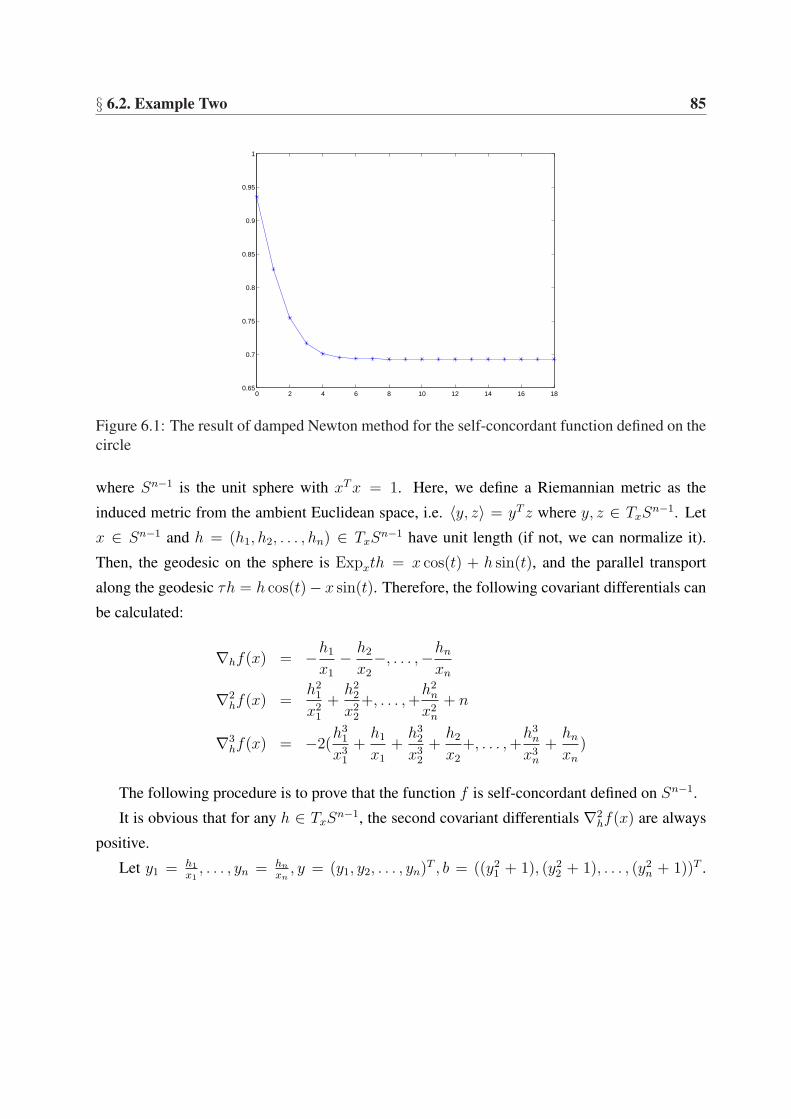
§ 6.2. Example Two 85
0 2 4 6 8 10 12 14 16 180.65
0.7
0.75
0.8
0.85
0.9
0.95
1
Figure 6.1: The result of damped Newton method for the self-concordant function defined on thecircle
where Sn−1 is the unit sphere with xT x = 1. Here, we define a Riemannian metric as the
induced metric from the ambient Euclidean space, i.e. 〈y, z〉 = yT z where y, z ∈ TxSn−1. Let
x ∈ Sn−1 and h = (h1, h2, . . . , hn) ∈ TxSn−1 have unit length (if not, we can normalize it).
Then, the geodesic on the sphere is Expxth = x cos(t) + h sin(t), and the parallel transport
along the geodesic τh = h cos(t)− x sin(t). Therefore, the following covariant differentials can
be calculated:
∇hf(x) = −h1
x1
− h2
x2
−, . . . ,−hn
xn
∇2hf(x) =
h21
x21
+h2
2
x22
+, . . . , +h2
n
x2n
+ n
∇3hf(x) = −2(
h31
x31
+h1
x1
+h3
2
x32
+h2
x2
+, . . . , +h3
n
x3n
+hn
xn
)
The following procedure is to prove that the function f is self-concordant defined on Sn−1.
It is obvious that for any h ∈ TxSn−1, the second covariant differentials ∇2
hf(x) are always
positive.
Let y1 = h1
x1, . . . , yn = hn
xn, y = (y1, y2, . . . , yn)T , b = ((y2
1 + 1), (y22 + 1), . . . , (y2
n + 1))T .

§ 6.2. Example Two 86
0 1 2 3 4 5 6 7 8 9−16
−14
−12
−10
−8
−6
−4
−2
0
Iteration number
log1
0d(x
,x* )
Figure 6.2: The result of damped Newton method for the self-concordant function defined onhigh-dimension sphere
Then, we have
(∇3hf(x))2
(∇2hf(x))3
=4(y3
1+, . . . , +y3n + y1 + · · ·+ yn)
(y21 + · · ·+ y2
n + n)3
= 4(y1(y
21 + 1) + · · ·+ yn(y2
n + 1))2
((y21 + 1) + · · ·+ (y2
n + 1))3
≤ 4(y21 + · · ·+ y2
n)
(y21 + 1) + · · ·+ (y2
n + 1)
≤ 4 (6.5)
Therefore, the function f is a self-concordant function defined on Sn−1 with Mf = 2.
We apply damped Newton and damped conjugate gradient algorithms to this problem. In
particular, n = 10. Figure 6.3 illustrates the result of the damped Newton method on function f .
This result also demonstrates the quadratic convergence of the damped Newton algorithm.
Figure 6.3 illustrates the result of the damped conjugate gradient method on function f . This
result also shows the superlinear convergence of the damped conjugate gradient method.

§ 6.3. Example Three 87
0 2 4 6 8 10 12−9
−8
−7
−6
−5
−4
−3
−2
−1
0
Iteration number
log1
0d(x
,x* )
Figure 6.3: The result of damped conjugate gradient method for the self-concordant functiondefined on high-dimension sphere
6.3 Example Three
In this subsection, we consider the problem of computing the center of mass of a set of given
points defined on the hyperboloid model. Before defining this problem, we first introduce the
geometric properties of the hyperboloid model. In Rn+1, consider the following quadratic form
Q,
Q(x) = −n∑
i=1
x2i + x2
n+1. (6.6)
Let A = diag(−1,−1, . . . ,−1︸ ︷︷ ︸n
, 1). Then Q can be represented in terms of A by
Q(x) = xT Ax. (6.7)
Given this quadratic form, the upper fold In of the hyperboloid is determined by the formula
In = x ∈ Rn+1|Q(x) = 1, xn+1 > 0. (6.8)
The set In can be regarded as a differentiable hypersurface in Rn+1 since it is an open subset
of the pre-image of a regular value of a differentiable function. In particular, it inherits from

§ 6.3. Example Three 88
Rn+1 a differentiable structure of dimension n. For any x ∈ In, the tangent space TxIn is
TxIn = X ∈ Rn+1|xT AX = 0. (6.9)
For any x ∈ In, we define a Riemannian metric on the tangent space of x by
〈X, Y 〉x = XT (−A)Y, X, Y ∈ TxIn. (6.10)
Given a point x ∈ In and a non-zero tangent vector X ∈ TxIn, the geodesic emanating from
x in the direction X is given by [6]
ExpxtX = xcosh(θt) +1
θXsinh(θt) (6.11)
where θ =√
XT (−A)X .
The intrinsic distance between x ∈ In and y ∈ In on this hyperboloid model is given by [73]
d(x, y) = arccosh(xT Ay). (6.12)
Recall that arccosh(t) = ln(t +√
t2 − 1) for t > 1. Since d(x, y) ≥ 0, we can expect that
xT Ay ≥ 1 holds for all x, y ∈ In. Since we require this result elsewhere, we prove it from first
principles.
Proposition 6.3.1. For any two points x, y ∈ In, there holds
xT Ay ≥ 1. (6.13)
Proof: Since x, y ∈ In, we have
−x21 − x2
2 − · · · − x2n + x2
n+1 = 1, (6.14)
−y21 − y2
2 − · · · − y2n + y2
n+1 = 1. (6.15)
Let p = x21 + x2
2 + · · · + x2n and q = y2
1 + y22 + · · · + y2
n. Since xn+1 > 0 and yn+1 > 0, it

§ 6.3. Example Three 89
follows from (6.14) and (6.15) that
xn+1 =√
1 + p, (6.16)
yn+1 =√
1 + q. (6.17)
Then, we obtain
xT Ay = −x1y1 − x2y2 − . . . xnyn + xn+1yn+1
=√
(1 + p)(1 + q)− x1y1 − x2y2 − . . . xnyn
≥√
1 + p + q + pq −√pq
≥√
1 + 2√
pq + pq −√pq
= 1 +√
pq −√pq
= 1. (6.18)
¤Consider the following optimization problem
arg minp∈In
f(p) =1
2
n∑i=1
d2(p, pi) =1
2
n∑i=1
arccosh2(pT Api) (6.19)
where pi ∈ In, i = 1, . . . ,m. The solution of (6.19) is called the Karcher mean [42] of the given
points p1, . . . , pm.
By computation, we obtain the first, second and third covariant derivatives of the cost function
at p ∈ In in the direction H ∈ TpIn by
∇Hf(p) = θ
m∑i=1
arccosh(pT Api)XT Api√
(pT (−A)pi)2 − 1, (6.20)
∇2Hf(p) = θ2
m∑i=1
[(XT Api)
2
(pT APi)2 − 1
+ arccosh(pT Api)pT Api[(p
T Api)2 − (XT Api)
2 − 1]
(pT APi)2 − 1)32
], (6.21)
∇3Hf(p) = θ3
m∑i=1
[XT Api
((pT APi)2 − 1)32
− (XT Api)3
((pT APi)2 − 1)52
]
(3pT Api(pT Ap2
i − 1)12 − arccosh(pT Api)(2p
T Ap2i + 1)) (6.22)

§ 6.3. Example Three 90
where θ =√
HT (−A)H and X = H/θ.
By Theorem 2.1 in Page 111 in [71], since In is simply connected, complete with negative
sectional curvature, the function f(p) in (6.19) is strictly convex. Hence, this implies that for all
p ∈ In and H ∈ TpIn
∇2Hf(p) > 0. (6.23)
For any p ∈ In, the gradient gradpf of f is given by
gradpf = (kT Ap)p− k (6.24)
where k =∑m
i=1arccos(pT Api)pi√
(pT (−A)pi)2−1.
To prove that f in (6.19) is self-concordant, we need several auxiliary inequalities.
Proposition 6.3.2. For any x ≥ 1, the following inequality holds.
1.
arccosh(x) ≤√
x2 − 1 ≤ xarccosh(x) (6.25)
where the equalities hold only at x = 1.
2.
3x√
x2 − 1 ≤ arccosh(x)(2x2 + 1) (6.26)
where the equality holds only at x = 1.
3.
(3x√
x2 − 1− arccosh(x)(2x2 + 1))2 ≤ 4(x2 − 1)(xarccosh(x))2 (6.27)
where the equality holds only at x = 1.
Proof:

§ 6.3. Example Three 91
1. Let g(x) =√
x2 − 1− arccosh(x) where x ≥ 1. Then it can be calculated that
g′(x) =x√
x2 − 1− 1√
x2 − 1
=x− 1√x2 − 1
. (6.28)
Therefore, when x > 1, we obtain
g′(x) > 0. (6.29)
Thus, g(x) is monotonically increasing with respect to x when x > 1. Since g is continuous
on x and g(1) = 0, we have
g(x) ≥ g(1) = 0. (6.30)
Hence, it follows from (6.30) that
arccosh(x) ≤√
x2 − 1 (6.31)
where the equality holds only at x = 1.
Similarly, we can prove that
√x2 − 1 ≤ xarccosh(x) (6.32)
where the equality holds only at x = 1.
2. Let g(x) = 3x√
x2 − 1− arccosh(x)(2x2 + 1) where x ≥ 1. Then it can be calculated
g′(x) = 3√
x2 − 1 +3x2
√x2 − 1
− 2x2 + 1√x2 − 1
− 4xarccosh(x)
= 4(√
x2 − 1− xarccosh(x)). (6.33)
In view of (6.25), we obtain
g′(x) < 0 (6.34)

§ 6.3. Example Three 92
where x > 1.
Thus, g(x) is monotonically decreasing with respect to x when x > 1. Since g is continu-
ous on x and g(1) = 0, we have
g(x) ≤ g(1) = 0. (6.35)
Hence, it follows from (6.40) that
3x√
x2 − 1 ≤ arccosh(x)(2x2 + 1) (6.36)
where the equality holds only at x = 1.
3. Let g(x) = (3x√
x2 − 1−arccosh(x)(2x2 +1))2−4(x2−1)(xarccosh(x))2 where x ≥ 1.
Then it can be calculated
g′(x) = 8(3x√
x2 − 1− arccosh(x)(2x2 + 1))√
x2 − 1
+ arccosh(x)(2xarccosh(x)− 4x2√
x2 − 1). (6.37)
By (6.25), when x > 1, we obtain
2xarccosh(x) < 4x2√
x2 − 1. (6.38)
In view of (6.26) and (6.38), since arccosh(x) > 0 when x > 1, we have
g′(x) < 0. (6.39)
where x > 1.
Thus, g(x) is monotonically decreasing with respect to x when x > 1. Since g is continu-
ous on x and g(1) = 0, we have
g(x) ≤ g(1) = 0. (6.40)
§ 6.3. Example Three 93
Hence, it follows from (6.40) that
(3x√
x2 − 1− arccosh(x)(2x2 + 1))2 ≤ 4(x2 − 1)(xarccosh(x))2 (6.41)
where the equality holds only at x = 1.
¤Without loss of generality, now we consider the following optimization problem
min f0(p) =1
2d2(p, p0) =
1
2arccosh(pT Ap0)
s.t. p ∈ In (6.42)
where p0 ∈ In is given. Similarly, we obtain the first, second and third covariant derivatives of
f0 as follows.
∇Hf0(p) = θarccosh(pT Ap0)XT Ap0√
(pT (A)p0)2 − 1, (6.43)
∇2Hf0(p) = θ2
[(XT Ap0)
2
(pT AP0)2 − 1
+ arccosh(pT Ap0)pT Ap0[(p
T Ap0)2 − (XT Ap0)
2 − 1]
((pT AP0)2 − 1)32
], (6.44)
∇3Hf0(p) = θ3
[XT Ap0
((pT AP0)2 − 1)32
− (XT Ap0)2
((pT AP0)2 − 1)52
]
(3pT Ap0((pT Ap0)
2 − 1)12 − arccosh(pT Ap0)(2(pT Ap0)
2 + 1)),
(6.45)
where θ =√
HT (−A)H and X = H/θ.
Lemma 10. Given any p ∈ In, and H ∈ TpIn, the following result holds:
(XT Ap0)2 ≤ (pT Ap0)
2 − 1 (6.46)
where θ =√
HT (−A)H , X = H/θ and X = 0 if H = 0.
Proof: For simplicity, let B = pT Ap0. If H = 0, since pT Ap0 ≥ 1 by Proposition 6.3.1, we

§ 6.3. Example Three 94
have
B2 − 1 ≥ 0 = (XT Ap0)2. (6.47)
Otherwise, consider two cases here.
Case one: p = p0. Then we have B = 1 and XT Ap0 = 0. Consequently, we obtain
B2 − 1 ≥ 0 = (XT Ap0)2. (6.48)
Case two: p 6= p0. Then we have B > 1 and XT Ap0 6= 0. Let γ(t) denote the geodesic
emanating from p in the direction H . Then we have γ(t) = ExpptH = pcosh(θt) + Xsinh(θt)
where θ =√
HT (−A)H and X = H/θ. Consider the function f0 in (6.42). In view of Equation
(1.2.2) of Theorem 1.2 in [42], we have
∇2Hf0(p) ≥ ‖H‖2
p. (6.49)
Substituting (6.44) into (6.49), we obtain
√B2 − 1−Barccosh(B)
(B2 − 1)32
(XT Ap0)2 +
Barccosh(B)√(B2 − 1)
≥ 1. (6.50)
It follows from (6.50) that
(XT Ap0)2 ≤ B2 − 1. (6.51)
This completes the proof of the lemma. ¤With the help of Proposition 6.3.2 and Lemma 10, we can show that f0 in (6.42) is self-
concordant.
Lemma 11. The function f0 in (6.42) is a self-concordant function defined on the n-dimensional
hyperboloid model with the constant Mf0 =√
1627
.
Proof: Given a point p = p0 and a tangent vector H ∈ TpIn, we have
∇2Hf(p) = ‖H‖2
p, (6.52)
∇3Hf(p) = 0. (6.53)

§ 6.3. Example Three 95
Then, it holds
|∇3Hf(p)| ≤
√16
27
(∇2
Hf(p)
) 32
. (6.54)
Otherwise, given a point p ∈ In, p 6= p0 and a nonzero tangent vector H ∈ TpIn, let
B = pT Ap0 and w = XT Ap0. Then we have
(∇3Hf0(p))2
(∇2Hf0(p))3
=
[w
(B2−1)32− w3
(B2−1)52
]2[3B√
B2 − 1− (2B2 + 1)arccosh(B)
]2
[√B2−1−Barccosh(B)
(B2−1)32
w2 + Barccosh(B)√B2−1
]3
=[3B
√B2 − 1− (2B2 + 1)arccosh(B)]2[(B2 − 1)w − w3]2√
B2 − 1[(√
B2 − 1−Barccosh(B))w2 + (B2 − 1)Barccosh(B)]3
=[3B
√B2 − 1− (2B2 + 1)arccosh(B)]2√
B2 − 1(Barccosh(B)−√B2 − 1)3
w2(B2 − 1− w2)2
[Barccosh(B)
Barccosh(B)−√B2−1(B2 − 1)− w2
]3 (6.55)
Let t = w2. Then we have the range of t by Lemma 10
0 ≤ t ≤ B2 − 1. (6.56)
For simplicity, let a = B2 − 1 and b = Barccosh(B)
Barccosh(B)−√B2−1(B2 − 1). By (6.25), we have
b > a > 0. (6.57)
Now we consider the following auxiliary function
π(t) =t(a− t)2
(b− t)3(6.58)
where t satisfies (6.56).

§ 6.3. Example Three 96
By computation, we obtain the first and second order derivatives of π
π′(t) =(a− t)[(2a− 3b)t + ab]
(b− t)4(6.59)
π′′(t) =(a− t)(2a− 3b)(b− t)− ((2a− 3b)t + ab)(b− 4a + 3t)
(b− t)5. (6.60)
Setting π′(t) = 0, it is easy to compute critical points t∗ of π
t∗ = a,
t∗ =ab
3b− 2a.
It is easy to see that these two critical points satisfy (6.56). Then substituting t∗ into (6.60), we
obtain
π′′(a) =3a
(b− a)3(6.61)
π′′(ab
3b− 2a) =
−3a(b− a)
(b− ab3b−2a
)4(6.62)
By (6.57), we obtain
π′′(a) > 0, (6.63)
π′′(ab
3b− 2a) < 0. (6.64)
Since π(t) is continuous on t, it follows from (6.64) that π achieves its maximum at t = ab3b−2a
.
By computation, we can get such maximum
π(ab
3b− 2a) =
4
27
a3
b2(b− a). (6.65)
Combining (6.55) and (6.65), we obtain
(∇3Hf0(p))2
(∇2Hf0(p))3
≤ 4
27
[3B√
B2 − 1− (2B2 + 1)arccosh(B)]2
(B2 − 1)(Barccosh(B))2(6.66)

§ 6.3. Example Three 97
In view of (6.27), it follows from (6.66) that
(∇3Hf0(p))2
(∇2Hf0(p))3
≤ 16
27. (6.67)
As a consequence, we conclude that f0 is self-concordant with Mf0 =√
1627
. ¤
Lemma 12. The function f in (6.19) is a self-concordant function defined on the n-dimensional
hyperboloid model with the constant Mf =√
1627
.
Proof: In view of Proposition 4.3.2 and Lemma 11, it is easy to conclude that f in (6.19) is
self-concordant with the constant Mf =√
1627
. ¤Since the function f in (6.19) is self-concordant, we are able to apply our damped Newton
and conjugate gradient algorithms to find the minimum of f on In. In particular, we take n = 19.
First, we consider building up the damped Newton algorithm for (6.19).
In view of (4.49), given a point p ∈ In, the Newton direction XN of f at p is the unique
tangent vector determined by
Hesspf(XN , H) = 〈−gradpf, H〉p for all tangent vectors H ∈ TpIn. (6.68)
By (4.6) and (6.21), we obtain
Hesspf(XN , H) =m∑
i=1
[1
(pT Api)2 − 1XT
NApiHT Api +
arccosh(pT Api)pT Api√
(pT Api)2 − 1
XTN(−A)H − arccosh(pT Api)p
T Api
((pT Api)2 − 1)32
]. (6.69)
Then, combining (6.68) and (6.69), we get
m∑i=1
[(1
(pT Api)2 − 1− arccosh(pT Api)p
T Api
((pT Api)2 − 1)32
)(XT
NApipTi App− pip
Ti AXN
)
+
(arccosh(pT Api)p
T Api√(pT Api)2 − 1
)XN = −gradpf (6.70)
Thus, the solution of the linear system (6.70) is the Newton direction of f at p which can be
used for the damped Newton method. To solve this linear system, we adopt the linear conjugate
gradient method modified directly from Golub and Van Loan [29] as follows.

§ 6.3. Example Three 98
Algorithm 16. (Linear Conjugate Gradient Algorithm)step 0: Given a point p ∈ In, compute R0 = −gradpf , and set P0 = R0 and k = 0.
step k: If k = n, then terminate. If k = 1, set
P1 = R0. (6.71)
Otherwise, compute
Qk =m∑
i=1
[(1
(pT Api)2 − 1− arccosh(pT Api)p
T Api
((pT Api)2 − 1)32
)(P T
k ApipTi App− pip
Ti APk
)
+
(arccosh(pT Api)p
T Api√(pT Api)2 − 1
)Pk, (6.72)
βk−1 =〈Rk−1, Rk−1〉p〈Rk−2, Rk−2〉p , (6.73)
Pk = Rk−1 + βk−1Pk−1, (6.74)
αk =〈Rk−1, Rk−1〉p〈Pk, Qk〉p , (6.75)
Xk = Xk−1 + αkPk, (6.76)
Rk = Rk−1 − αkQk. (6.77)
Increment k and repeat until k = n.
After n steps, Algorithm 16 generates a finite sequence X1, . . . , Xn and the Newton
direction of f at p is given by
XN = Xn. (6.78)
Now, we are able to construct the damped Newton method for solving (6.19).
Algorithm 17. step 0: Randomly generate an initial point p0 ∈ In and compute gradp0f . Set
k = 0.
step k: If gradpkf = 0, then terminate. Otherwise, compute XNpk
using Algorithm 16. Then,

§ 6.3. Example Three 99
compute
λk = ∇2XNpk
f(pk), (6.79)
tk =1
1 + λk
, (6.80)
pk+1 = pk cosh
(√XNpk
(−A)XNpktk
)+
XNpk√XNpk
(−A)XNpk
sinh
(√XNpk
(−A)XNpktk
),
(6.81)
where ∇2XNpk
f(pk) is from (6.21).
Increment k and repeat until convergence.
On the other hand, the damped conjugate gradient method for solving (6.19) is given as
follows.
Algorithm 18. (Conjugate Gradient Algorithm)step 0: Select an initial point p0 ∈ In, compute H0 = G0 = −(gradp0
f) by (6.85), and set
k = 0.
step k: If gradpkf = 0, then terminate. Otherwise, compute
λk =−∇Hk
f(pk)√∇2
Hkf(pk)
, (6.82)
tk =λk
(1 + λk)√∇2
Hkf(pk)
, (6.83)
pk+1 = pk cosh
(√Hk(−A)Hktk
)+
Hk√Hk(−A)Hk
sinh
(√Hk(−A)Hktk
), (6.84)
Gk+1 = −gradpk+1f, (6.85)
γk+1 =〈Gk+1, Gk+1〉pk+1
〈Gk, Hk〉pk
, (6.86)
Hk+1 = Gk+1 + γk+1τpkpk+1Hk, (6.87)
where τpkpk+1is the parallel transport with respect to the geodesic from pk to pk+1. If k + 1
mod n− 1 = 0, set Hk+1 = Gk+1. Increment k and repeat until convergence.

§ 6.3. Example Three 100
0 2 4 6 8 10 12 14 16 18−14
−12
−10
−8
−6
−4
−2
0
2
Iteration number
log1
0(f−
f* )
Damped Newton method
Figure 6.4: The result of the the damped Newton method for the self-concordant function definedon the Hyperboloid model
Figure 6.5 illustrates the result of the damped Newton method and conjugate gradient method
on function f in (6.19). Table 6.2 shows the simulation time and accuracy using the damped
conjugate gradient and Newton methods. From Figure 6.5, it can be see that the damped Newton
method converges to the minimum quadratically, but the damped conjugate gradient method gets
to the minimum super-linearly. Although the damped conjugate gradient method requires more
steps, due to avoid computing the linear system, it costs less time than the damped Newton
method, seen from Table 6.2.
algorithm time(second) accuracydamped conjugate gradient method 0.062 10−5
damped Newton method 0.313 10−5
Table 6.2: Simulation time and accuracy

§ 6.3. Example Three 101
0 5 10 15 20 25−10
−8
−6
−4
−2
0
2
Iteration number
log1
0((f
(xk))
−f(
x* ))
Damped conjugate gradeint method
Figure 6.5: The result of the damped conjugate gradient method for the self-concordant functiondefined on the Hyperboloid model

Part III
The Quasi-Newton Method
102

Chapter 7
A Quasi-Newton Method On SmoothManifolds
7.1 Introduction
Background The quasi-Newton method is preferred by engineers since it has lower com-
putational cost than the Newton method and super-linear convergence rate. As we mentioned in
Chapter 1, Gabay has generalized the quasi-Newton method to Riemannian manifolds. However,
in recent years, the non-Riemannian methods on smooth manifolds have drawn more attentions
due to their prominent advantages. To our best knowledge, we are not aware of any publications
generalizing quasi-Newton methods on the non-Riemannian cases. Hence, we are motivated to
develop a non-Riemannian quasi-Newton method for the optimization on smooth manifolds.
Our work In this chapter, we present a numerical non-Riemannian quasi-Newton method
on smooth manifolds. This method is proved to converge to the local minimum of the cost func-
tion. The super-linear convergence rate was demonstrated by simulation results on the Grass-
mann manifold.
Chapter outline The rest of this chapter is organized as follows. We first give the prelim-
inaries associated with smooth manifolds in Section 7.2. Then a non-Riemannian quasi-Newton
method is presented for the optimization on smooth manifolds and it is proved to converge to the
minimum of the cost function in Section 7.3. In Section 7.4 simulation results show our method
has the super-linear convergence rate. This is followed by the conclusions in Section 7.5.
103

§ 7.2. Preliminaries 104
7.2 Preliminaries
In this section, we briefly introduce notations and concepts of local parametrization for
smooth manifolds. For more details, see [46]. Let M be a smooth n−dimensional manifold.
Then for every point p ∈ M there exists a smooth map
ψp : Ωp ⊂ Rn → Up ⊂ M, ψp(0) = p (7.1)
where Up is an open neighborhood of p and Ωp an open subset of Rn around 0. Such a map
is called a local parametrization around p. We use the triple (ψp, Up, Ωp) to denote the local
parametrization around p. Let f : M → R be a real-valued smooth function defined on a smooth
manifold M . Given a point p ∈ M and a local parametrization (ψp, Up, Ωp) around p, then the
composition of f and ψp is called the local cost function and denoted by fψp. For simplification,
let gp : Ωp → R denote such local cost function satisfying
gp(x) = f(ψp(x)). (7.2)
7.3 Quasi-Newton Method On Smooth Manifolds
In this section, we develop a quasi-Newton method for the optimization of smooth functions
defined on smooth manifolds.
Before we give our method, we review the BFGS method [64] for the optimization in Eu-
clidean space. Consider the following optimization problem
minx∈Rn
f : Rn → R : x → f(x). (7.3)
Let f ′(x) denote the first derivative of f at x. Then the BFGS algorithm for solving (7.3)
goes as follows.
Algorithm 19. (BFGS Algorithm in Euclidean Space)step 0: Select an initial point x0 and set B0 = In where In denotes the n−dimensional
identity matrix and k = 0. Compute H0 = −B−10 f ′(x0).
step k: If f ′(xk) = 0, then terminate. Otherwise, compute the step-size λk as follows.
λk = 2−l (7.4)

§ 7.3. Quasi-Newton Method On Smooth Manifolds 105
where l is the smallest positive integer such that
f(λkHk) ≤ f(xk) + c1λkHTk f ′(xk), (7.5)
HTk f ′(λkHk) ≥ c2H
Tk f ′(xk), (7.6)
where 0 < c1 < c2 < 1.
Set
xk+1 = xk + λk+1Hk, (7.7)
sk = xk+1 − xk, (7.8)
yk = f ′(xk+1)− f ′(xk), (7.9)
Bk+1 = Bk +yky
Tk
〈yk, sk〉 +Bksk(Bksk)
T
〈Bksk, sk〉 , (7.10)
Hk+1 = −B−1k+1f
′(xk+1). (7.11)
Increment k and repeat until convergence.
In Algorithm 19, Equation (7.5) and (7.6) form the Wolfe conditions [61] used to determine
the appropriate step-size in the line search. Equation (7.10) provides an approximation to the
Hessian of f over successive iterations using only its first order information. Moreover, Algo-
rithm 19 turns out to has super-linear convergence in [64].
Now, we consider to generalize the BFGS method for the optimization on smooth manifolds.
Let M be a smooth n−dimensional manifold. For p ∈ M , let the triple (ψp, Up, Ωp) be the local
parametrization around p. Consider the following optimization problem
minp∈M
f : M → R : p → f(p). (7.12)
For any p ∈ M and the local parametrization (ψp, Up, Ωp) around p, let gp(x) denote the local
cost function of f . Moreover, let g′p(x) and g′′p(x) denote the first and second derivatives of gp(x)
with respect to x respectively. Then a quasi-Newton method is developed for solving (7.12) as
follows.
Algorithm 20. (Quasi-Newton Algorithm)step 0: Select an initial point p0 ∈ M and set B0 = In where In denotes n−dimensional
identity matrix and k = 1. Compute H0 = −B−10 g′p0
(0).

§ 7.3. Quasi-Newton Method On Smooth Manifolds 106
step k: If g′pk(0) = 0, then terminate. Otherwise, compute the step-size λk as follows.
λk = 2−l (7.13)
where l is the smallest positive integer such that
gpk(λkHk) ≤ gpk
(0) + c1λkHTk g′pk
(0), (7.14)
HTk g′pk
(λkHk) ≥ c2HTk g′pk
(0), (7.15)
where 0 < c1 < c2 < 1.
Set
xk+1 = λk+1Hk, (7.16)
sk = xk+1, (7.17)
yk = g′pk(xk+1)− g′pk
(0), (7.18)
Bk+1 = Bk +yky
Tk
〈yk, sk〉 +Bksk(Bksk)
T
〈Bksk, sk〉 , (7.19)
pk+1 = ψpk(xk+1), (7.20)
Hk+1 = −B−1k+1g
′pk+1
(0). (7.21)
Increment k and repeat until convergence.
In Algorithm 21, Equation (7.14) and (7.15) form the Wolfe conditions [61] used to deter-
mine the appropriate step-size in the line search. They facilitate the proof of the convergence of
Algorithm 21.
Now, we consider proving the convergence of Algorithm 21. Before we do that, we need an
assumption.
Assumption 4. There exist
1. a point p0 ∈ M which defines a sub-level set K = p ∈ M∣∣f(p) ≤ f(p0);
2. local parametrization ψp for all p ∈ K, defined in (7.1);
such that for all p ∈ K, x ∈ Ωp and any u ∈ Rn,
α‖u‖2 ≤ uT g′′pk(x)u ≤ β‖u‖2 (7.22)
§ 7.3. Quasi-Newton Method On Smooth Manifolds 107
where β, α > 0 are constants.
Assumption 4 implies that for each p ∈ K, we can find a local parametrization such that
the local cost function determined by it is convex on its local Euclidean space. For example,
consider the convex function defined on Riemannian manifolds in [70]. Viewing the geodesics
as one kind of local parametrization, then according to the definition of convex functions on
Riemannian manifolds, we can find a neighborhood around the local minimum such that the
local cost functions are convex.
Equation (7.19) gives the formula which approximates the Hessian of the local cost function.
It is worth noting that Equation (7.19) has the same expression as the BFGS update formula
(7.10). Since the local cost function satisfies (7.22), according to Theorem 1.6.7 in [64], we
conclude that if Bk is symmetric positive-definite, then Bk+1, given by (7.19), is also symmetric
positive-definite. Furthermore, since the initial matrix B0 is identity, it is easy to see the matrix
in Bk generated by Algorithm (21) is always symmetric positive-definite. As a result, at each
step, Algorithm (21) yields a descent step. In addition, in view of Equation (28f) and (29) in
[64], the trace and determinant of Bk+1 are given by
tr(Bk+1) = tr(Bk) +‖yk‖2
〈yk, sk〉 −‖Bksk‖〈Bksk, sk〉 , (7.23)
det(Bk+1) = det(Bk)〈yk, sk〉〈Bksk, sk〉 . (7.24)
To show the global convergence of Algorithm 21, we follow the frameworks in [8]. Initially,
motivated by (7.23) and (7.24), we obtain the following lemmas, which lead to the convergence
result.
Lemma 13. Let the cost function f : M → R in (7.12) satisfy Assumption 4. Then given
p0 ∈ K, applying Algorithm 21 to minimize f , we have
‖yk‖2
〈yk, sk〉 ≤ β (7.25)
where sk and yk are defined by (7.66) and (7.18) respectively.

§ 7.3. Quasi-Newton Method On Smooth Manifolds 108
Proof: Consider the local cost function gpkdefined on Ωpk
. Since xk+1 ∈ Ωpk, then we have
∫ 1
0
g′′pk(tsk)dtsk = g′pk
(xk+1)− g′pk(0)
= yk. (7.26)
Let Bk+1 =∫ 1
0g′′pk
(tsk)dt. Then it follows from (7.26) that
Bk+1sk = yk. (7.27)
In addition, for any v 6= 0 ∈ Rn, we have
vT Bk+1v = vT
∫ 1
0
g′′pk(tsk)dtv
≤∫ 1
0
β‖v‖2dt
= β‖v‖2 (7.28)
where the inequality comes from (7.22).
Then it follows from (7.28) that
vT Bk+1v
‖v‖2≤ β. (7.29)
Since Bk+1 is symmetric and positive definite, let v = B12k+1. Combining (7.27) and (7.29),
we obtain
‖yk‖2
〈yk, sk〉 ≤ β. (7.30)
¤
Lemma 14. Let the cost function f : M → R in (7.12) satisfy Assumption 4. Then given
p0 ∈ K, applying Algorithm 21 to minimize f , there exists a constant A > 0 such that
tr(Bk+1) ≤ Ak. (7.31)

§ 7.3. Quasi-Newton Method On Smooth Manifolds 109
Proof: By (7.23), it is easy to see that
tr(Bi+1) ≤ tr(Bi) +‖yi‖2
〈yi, si〉 . (7.32)
Summing up the inequalities (7.32) for i = 0, 1, . . . , k, we have
trBk+1 ≤ tr(B0) +k∑
i=0
‖yi‖2
〈yi, si〉≤ tr(B0) + βk
≤ Ak (7.33)
where A = tr(B0) + β.
This completes the proof of the lemma. ¤
Lemma 15. Let the cost function f : M → R in (7.12) satisfy Assumption 4. Then given
p0 ∈ K, applying Algorithm 21 to minimize f , there exists a constant L > 0 such that
det(Bk+1) ≥ β
k∏i=0
‖g′pi(0)‖2〈yi, si〉
L〈g′pi(0), si〉 . (7.34)
Proof: Multiplying (7.24) from i = 1, . . . , k, we have
det(Bk+1) = det(B0)k∏
i=0
〈yi, si〉〈Bisi, si〉 . (7.35)
It follow from (7.23) and (7.30) that
tr(Bi+1)− tr(Bi) +‖Bisi‖〈Bisi, si〉 =
‖yi‖2
〈yi, si〉≤ β. (7.36)
Then, by (7.36), we have
β + tr(Bi)− tr(Bi+1) ≥ ‖Bisi‖2
〈Bisi, si〉 . (7.37)

§ 7.3. Quasi-Newton Method On Smooth Manifolds 110
Summing up (7.37) from i = 0, 1, . . . , k, we obtain
k∑i=0
‖Bisi‖2
〈Bisi, si〉 ≤ kβ + trB0 − tr(Bk+1)
≤ kβ + tr(B0). (7.38)
Let L = β + tr(B0). Then it follows from (7.38) that
1
k + 1
k∑i=0
‖Bisi‖2
〈Bisi, si〉 ≤ L. (7.39)
Recall that given k positive numbers z1, . . . zk, then the arithmetic mean is greater than the
geometric mean. That is
(1
k
k∑i=1
ai
)k
≥k∏
i=1
ai. (7.40)
Therefore, by (7.39), we obtain
Lk+1 ≥k∏
i=0
‖Bisi‖2
〈Bisi, si〉 . (7.41)
Multiplying (7.35) and (7.41), we have
Lk+1 det(Bk+1) ≥k∏
i=0
‖Bisi‖2〈yi, si〉〈Bisi, si〉2 . (7.42)
In view of (7.65), (7.66) and (7.21), we get
Bisi = −λi+1g′pi
(0). (7.43)
Substituting (7.43) into (7.42), we obtain
Lk+1 det(Bk+1) ≥ βk∏
i=0
‖g′pi(0)‖2〈yi, si〉〈g′pi
(0), si〉 . (7.44)

§ 7.3. Quasi-Newton Method On Smooth Manifolds 111
Thus, it follow from (7.44) that
det(Bk+1) ≥ β
k∏i=0
‖g′pi(0)‖2〈yi, si〉
L〈g′pi(0), si〉 . (7.45)
As a result, this lemma follows. ¤The following theorem show that Algorithm 21 converges to the minimum of f in (7.12)
when it satisfies Assumption (4).
Theorem 7.3.1. Let the cost function f : M → R in (7.12) satisfy Assumption 4. Then given
p0 ∈ K, applying Algorithm 21 to minimize f , it holds
limk→∞
inf ‖g′pk(0)‖ = 0. (7.46)
Proof: By definition,
〈yk, sk〉 = 〈g′pk(xk+1)− g′pk
(0), sk〉= 〈g′pk
(xk+1), sk〉 − 〈g′pk(0), sk〉. (7.47)
In view of (7.15), it follows from (7.47) that
〈yk, sk〉 ≥ (c2 − 1)〈g′pk(0), sk〉. (7.48)
By (7.14), we have
gpk(xk+1)− gpk
(0) ≤ c1〈g′pk(0), sk〉. (7.49)
Substituting (7.48) and (7.49)into (7.34), we obtain
det(Bk+1) ≥ β
k∏i=0
c1‖g′pi(0)‖2(1− c2)
L(gpk(xk+1)− gpk
(0))
= βθk+1‖g′pi
(0)‖2
gpk(xk+1)− gpk
(0)(7.50)
where θ = c1(1−c2)L
.

§ 7.3. Quasi-Newton Method On Smooth Manifolds 112
Using the original cost function f , by (7.50) and (7.40), we have
det(Bk+1) ≥ βθk+1
∏ki=0 ‖g′pi
(0)‖2
∏ki=0(f(pi+1)− f(pi))
≥ βθk+1
∏ki=0 ‖g′pi
(0)‖2
( 1k+1
∑ki=0(f(pi+1)− f(pi)))k
≥ β(L(k + 1))k+1
(f(p0)− f(p∗))k+1
k∏i=0
‖g′pi(0)‖2
≥ β(S(k + 1))k+1
k∏i=0
‖g′pi(0)‖2 (7.51)
where S = Lf(p0)−f(p∗) and p∗ is the local minimum.
Applying (7.40) again, by (7.51) we have
β(S(k + 1))k+1
k∏i=0
‖g′pi(0)‖2 ≤ det(Bk+1)
≤ (1
ntr(Bk))
≤ (1
nA(k + 1))n
≤ N(k + 1)n (7.52)
where the second inequality comes from Lemma (14) and N = (An)n.
Assume that (7.46) does not hold. That is there exists an ε > 0 such that for all k
‖g′pk(0)‖2 ≥ ε > 0. (7.53)
As a result of (7.53), in view of (7.52), we obtain
β(Sε(k + 1))k+1 ≤ N(k + 1)n (7.54)
which is impossible when k →∞ due to an exponential growing faster than a polynomial.
Consequently, this theorem follows. ¤

§ 7.4. Numerical Example 113
7.4 Numerical Example
In this section, we apply our quasi-Newton algorithm to find the dominant eigenspace of a
real symmetric matrix.
Let A ∈ Rn×n be a symmetric matrix, i.e. A = AT . Let λ1 ≥ λ2 ≥ · · · ≥ λp ≥ · · · ≥ λn
be the eigenvalues of A. Our aim is to find the subspace of Rn spanned by the eigenvectors
corresponding to the p largest eigenvalues λ1, . . . , λk. This subspace is called the dominant
eigenspace of A. To solve this problem, the natural way is to consider minimizing a cost function
defined on the Grassmann manifold.
Recall that the Grassmann manifold Gr(n, p) is defined as the set of all p−dimensional sub-
spaces of Rn. Let St(n, p) denote the Stiefel manifold defined as all matrices X ∈ Rn×p sat-
isfying XT X = Ip where Ip is the p−dimensional identity matrix. Let X ∈ St(n, p) and bXcdenote the subspace spanned by the columns of X . Then we have bXc ∈ Gr(n, p). The Grass-
mann manifold Gr(n, p) can be thought of as a quotient manifold of the Stiefel manifold. This
is explained as follows. Given two points X, Y ∈ St(n, p), we say X and Y are equivalent,
denoted by X ≡ Y if there exists a unitary matrix Q such that Y = XQ. It is easy to see that
X ≡ Y if and only if bXc = bY c. Thus, there exists a one-to-one correspondence between
points on the Grassmann manifold Gr(n, p) and equivalence classes of St(n, p). Given a point
X ∈ St(n, p), the tangent space TbXcGr(n, p) at bXc ∈ Gr(n, p) is given by
TbXcGr(n, p) = Z ∈ Rn×p : Z = X⊥B, B ∈ R(n−p)×p (7.55)
where X⊥ ∈ R(n−p)×p means the orthogonal complement of X and satisfies [X X⊥]T [X X⊥] =
In where In is the n−dimensional identity matrix.
In [53], Manton proposed a general framework for optimizing cost functions defined on
manifolds. As an example of how to apply the framework, the same paper considered local
parametrizations on the Grassmann manifold based on projections. Let X ∈ Rn×p be a matrix
with the rank p. Then the projection operator π : Rn×p → Gr(n, p) onto the Grassmann manifold
Gr(n, p) is defined by
π(X) =
⌊arg min
Q∈St(n,p)‖X −Q‖F
⌋. (7.56)
Then, given X ∈ St(n, p) and X⊥ - the orthogonal complement of X , in view of (7.55) and
(7.56), the local parametrization ψbXc : R(n−p)×p → Gr(n, p) around bXc ∈ Gr(n, p) is given
§ 7.4. Numerical Example 114
by
ψbXc(B) = π(X + X⊥B). (7.57)
Consider the following optimization problem:
min f : Gr(n, p) → R, bXc 7→ −tr(XT AX) (7.58)
where X ∈ St(n, p) and A = AT . The solution of (7.58) is the dominant eigenspace of A.
In view of (7.57), the local cost function gbXc : R(n−p)×p → R around bXc ∈ Gr(n, p) is
determined by
gbXc(B) = f ψbXc(B) = f(π(X + X⊥B)). (7.59)
By Proposition 22 in [53], an easy computation shows that
g′bXc(0) = −XT⊥AX, (7.60)
g′bXc(B) = −XT⊥A(X + X⊥B). (7.61)
Let vec(X) denote the vector by stacking the columns of the matrix X into a vector . Then,
the proposed quasi-Newton method for (7.58) goes as follows.
Algorithm 21. (Quasi-Newton Algorithm)step 0: Select an initial point X0 ∈ St(n, p) and set G0 = I(n−p)p where I(n−p)p denotes
(n − p)p−dimensional identity matrix and k = 1. Compute H0 = −G−10 vec(g′bX0c(0)) and set
H0 = uvec(H0) where uvec forms an n× p matrix in the reverse manner to the vec operator.
step k: If g′bXkc(0) = 0, then terminate. Otherwise, compute the step-size λk as follows.
λk = 2−l (7.62)
where l is the smallest positive integer such that
gbXkc(λkHk) ≤ gbXkc + c1λktr(HTk g′bXkc(0)), (7.63)
tr(HTk g′bXkc(λkHk)) ≥ c2tr(H
Tk g′bXkc(0)), (7.64)

§ 7.4. Numerical Example 115
0 5 10 15 20 25 30−9
−8
−7
−6
−5
−4
−3
−2
−1
0
Iteration number
log1
0(f(
Xk)−
f(X
* ))
The Newton MethodThe Steepest Decent MethodThe Quasi−Newton Method
Figure 7.1: The result of Quasi-Newton Method compared against the Newton method and steep-est decent method
where 0 < c1 < c2 < 1.
Set
Bk+1 = λk+1Hk, (7.65)
sk = vec(Bk+1), (7.66)
yk = vec(g′bXkc(Bk+1))− vec(g′bXkc(0)), (7.67)
Gk+1 = Gk +yky
Tk
〈yk, sk〉 +Gksk(Gksk)
T
〈Gksk, sk〉 , (7.68)
Xk+1 = π(Bk+1), (7.69)
Hk+1 = −G−1k+1g
′bXk+1c(0), (7.70)
Hk+1 = uvec(Hk+1), (7.71)
where π in (7.69) is defined in (7.56).
Increment k and repeat until convergence.
Figure 7.1 describes the result of applying our quasi-Newton method to solve (7.58). In
particular, we take n = 10, p = 6. This result demonstrates that the proposed quasi-Newton
method has super-linear convergence rate.

§ 7.5. Conclusions 116
7.5 Conclusions
In this chapter, we have presented a novel non-Riemannian quasi-Newton algorithm for the
optimization on smooth manifolds. This algorithm is developed based on the local parametriza-
tion and proved to converge to the local minimum of the cost function. Furthermore, this al-
gorithm is applied to minimize a cost function on the Grassmann manifold and the simulation
results show the super-linear convergence of our method.
Bibliography
[1] S. Abe, J. Kawakami, and K. Hirasawa. Solving inequality constrained combinatorial opti-
mization problems by the hopfield neural networks. Neural Networks, 5:663–670, 1992.
[2] P. A. Absil, R. Mahony, and R. Sepulchre. Riemannian geometry of grassmann manifolds
with a view on algorithmic computation. Acta Applicandae Mathematicae, 80(2):199220,
Jan. 2004.
[3] R. L. Adler, M. Dedieu J-P, Y. Joesph, M. Martens, and M. Shub. Newton’s method on
riemannian manifolds and a geometric model for the human spine. IMA J. Numerical
Analysis, 22:359–390, 2002.
[4] F. Alizadeh. Interior point methods in semidefinite programming with applications to com-
binatorial optimization. SIAM Jounal on Optimization, 5:13–51, 1995.
[5] F. Alizadeh, J. A. Haeberly, and M. Overton. Primal-dual interior point methods for
semidefinite programming: convergence rates, stabilibty, and numerical analysis. SIAM
Journal on Optimization, 8:746–768, 1998.
[6] R. Benedetti and C. Petronio. Lectures on Hyperbolic Geometry. Springer-Verlag, Berlin,
1992.
[7] L. Blum, F. Cucker, M. Shub, and S. Smale. Complexity and Real Computation. Springer-
Verlag, New York, 1998.
[8] J. F. Bonnans, J. C. Gilbert, C. Lemarechal, and C. A. Sagastizabal. Numerical Optimiza-
tion: Theoretical and Practical Aspects. Springer Verlag, New York, NY, 2003.
[9] S. Boyd, L. E. Ghaoui, and V. Balakrishnan. Linear Matrix Inequalities and Control Theory.
studies in applied mathematics 15. SIAM, Philadelphia, 1994.
117

BIBLIOGRAPHY 118
[10] S. Boyd and L. Vandenberghe. Convex Optimization. Cambridge University Press, Cam-
bridge, 2004.
[11] I. Brace. Optimisation on Manifolds with Applications. PhD thesis, University of Mel-
bourne, Melbourne, March 2006.
[12] I. Brace and J. H. Manton. An improved BFGS-on-manifold algorithm for computing
weighted low rank approximations. In Proceedings of the 17th International Symposium
on Mathematical Theory of Networks and Systems, Kyoto, Japan, 2006.
[13] R. W. Brockett. Differential geometry and the design of gradient algorithms. In ED. R.
Green and S. T. Yau, editors, Proceedings of the Symposium on Pure Mathematics, pages
69–92, Providence, RI, 1993.
[14] C. B. Brown and M. C. Bartholomew-Biggs. Some effective methods for unconstrained
optimization based on the solution of sytems of ordinary differential equations. Jounral on
Optimization Theory and Applications, 67:211–224, 1989.
[15] C. G. Broyden. A new double-rank minimization algorithm. Notices of the American
Mathematical Society, 16:670, 1969.
[16] C. G. Broyden. The convergence of a class of double-rank minimization algorithms. IMA
Journal of Applied Mathematics, 6(3):222–231, 1970.
[17] W. Davidon. Technical report anl-5990. Technical report, Argonne National Laboratory,
1959.
[18] P. Dedieu, J.-P. Priouret and G. Malajovich. Newton’s method on Riemannian manifolds:
Covariant alpha-theory. IMA Journal of Numerical Analysis, 23:395–419, 2003.
[19] A. Edelman, T. Arias, and S. T. Smith. The geometry of algorithms with orthogonality
constraints. SIAM Journal on Matrix Analysis and Applications.
[20] L. Faybusovich. Infinite dimensional semidefinite programming: regularized determinants
and self-concordant barriers. Fields Institute Communications, 8:39–49, 1998.
[21] R. Fletcher. A new approach to variable metric algorithms. Computer Journal, 13:317–322,
1970.

BIBLIOGRAPHY 119
[22] R. Fletcher. A nonlinear programming problem in statistics (educational testing). SIAM
Jounal on Scientific and Statistical Computing, 2:257–267, 1981.
[23] R. Fletcher. Practical Methods of Optimization, Vol I: Unconstrained Optimization. Wiley,
New York, 1987.
[24] R. Fletcher and C. M. Reeves. Functions minimization by conjugate gradients. Computer
Journal, 7:149–154, 1964.
[25] D. Gabay. Minimizing a differentiable function over a differentiable manifold. Journal of
Optimization Theory and Applications, 37(2):177–219, 1982.
[26] P. E. Gill, W. Murray, A. Saunders, and M. H. Wright. On projected newton methods for
linear programming and an equivalence to karmarkars projective method. Math. Program.,
36:183–209, 1986.
[27] F. Glineur. Improving complexity of structured convex optimization problems using self-
concordant barriers. European Jouranl of Operational Research, 143:291–310, 2002.
[28] D. Goldfarb. A family of variable-metric methods derived by variational means. Mathe-
matics of Computation, 24(109):23–26, 1970.
[29] G. H. Golub and C. F. V. Loan. Matrix computations. Johns Hopkins University Press,
Baltimore, MD, 1996.
[30] S. Helgason. Differential Geometry, Lie Groups, and Symmetric Spaces. Academic Press,
New York, 1978.
[31] C. Helmberg, F. Rendl, R. Vanderbei, and H. Wolkowicz. An interior-point method for
semidefinite programming. SIAM Jounal on Optimization, 6:342–361, 1996.
[32] U. Helmke, K. Huper, P. Lee, and J. B. Moore. Essential matrix estimation via newton-type
methods. In Proceedings of the MTNS, Leuven, 2004.
[33] U. Helmke, K. Huper, and J. B. Moore. Quadratically convergent algorithms for optimal
dextrous hand grasping. IEEE Trans. Robot. Automat., 18(2):38–146, Apr. 2002.
[34] U. Helmke and J. B. Moore. Optimization and Dynamical Systems. Springer-Verlag, Lon-
don, 1996.

BIBLIOGRAPHY 120
[35] U. Helmke, S. Riardo, and J. B. Yoshizawa. Newton’s algorithm in Euclidean jordan alge-
bras, with applications to robotics. Communications in Information and Systems, 2(3):283–
297, 2002.
[36] W. Yan, U. Helmke, and J. B. Moore. Global analysis of Oja’s flow for neural networks.
IEEE Transactions on Neural Networks, 5:674–683, 1993.
[37] D. den Hertog. Interior Point Approach to Linear, Quadratic and Convex Programming.
Mathematics and Its Applications 277. Kluwer Academic Publishers, London, 1994.
[38] M. R. Hestenes and E. Stiefel. Methods of conjugate gradients for solving linear systems.
Jouranl of Research of the National Bureau of Standards, 49:409–436, 1952.
[39] K. Huper and J. Trumpf. Newton-like methods for numerical optimization mainifolds. In
Proceedings of the 38th Asilomar Conference on Signals, Systems and Computers, pages
136–139, Asilomar Hotel and Conference Grounds, California, USA, 2004.
[40] D. Jiang, J. B. Moore, and H. Ji. Self-concordant functions for optimization on smooth
manifolds. In Proceedings of the 43rd IEEE Conference on Decision and Control, pages
3631–3636, Bahamas, Dec. 2004.
[41] D. Jiang and J. Wang. A recurrent neural network for real-time semidefinite programming.
IEEE Transactions on Neural Networks, 10:81–93, 1999.
[42] H. Karcher. Riemannian center of mass and mollifier smoothing. Communication on Pure
and Applied Mathematics, 30:509–541, 1977.
[43] N. Karmarkar. A new polynomial time algorithm for linear programming. Combinatorica,
4:373–395, 1984.
[44] M. P. Kennedy and L. O. Chua. Neural network for nonlinear programming. IEEE Trans.
Circuits Syst., 35:554–562, 1988.
[45] L. G. Khatchiyan. A polynomial algorithm in linear programming. Soviet Mathematics
Doklady, 20:191–194, 1979.
[46] S. Lang. Fundamentals of Differential Geometry. Springer, New York, 1999.

BIBLIOGRAPHY 121
[47] P. Y. Lee. Geometric Optimization for Computer Vision. PhD thesis, Australian National
University, Canberra, April 2005.
[48] D. G. Luenberger. The gradient projection method along geodesics. Management Science,
18:620–631, 1972.
[49] D. G. Luenberger. Introduction to Linear and Nonlinear Programming. Reading, 1973.
[50] Y. Ma, J. Kosecka, and S. Sastry. Optimization criteria and geometric algorithms for motion
and structure estimation. International Journal of Computer Vision, 44(3):219–249, 2001.
[51] R. Mahony. Optimization Algorithms on Homogeneous Spaces. PhD thesis, Australian
National University, Canberra, March 1994.
[52] R. Mahony. The constrained newton method on a lie group and the symmetric eigenvalue
problem. Linear Algebra and Its Applications, 248:67–89, 1996.
[53] J. H. Manton. Optimisation algorithms exploting unitary constraints. IEEE Transactions
on Signal Processing, 50(3):635–650, Mar. 2002.
[54] J. H. Manton. On the various generalisations of optimisation algrithms to manifolds. In
Sixteenth International Symposium on Mathematical Theory of Networks and Systems,
Katholieke Universiteit Leuven, Belgium, 2004.
[55] J. H. Manton. A centroid (karcher mean) approach to the joint approximate diagonalisation
problem: The real symmetric case. Digital Signal Processing, 16:468–478, 2006.
[56] L. Nazareth. A relationship between BFGS and conjugate gradient algorithms and its im-
plications for new algorithms. SIAM Journal on Numerical Analysis, 16(5):794–800, Oct.
1979.
[57] Y. Nesterov. Introductory Lectures on Convex Optimization: A Basic Course. Kluwer
Academic Publishers, Massachusetts, 2004.
[58] Y. Nesterov and A. Nemirovskii. Interior-Point Polynomial Algorithms in Convex Program-
ming. studies in applied mathematics 13. SIAM, Philadelphia, 1994.
[59] Y. Nesterov and M. Todd. On the Riemannian geometry defined by self-concordant barriers
and interior-point methods. Foundations of Computational Mathematics, pages 333–361,
2002.

BIBLIOGRAPHY 122
[60] Y. Nishimori and S. Akaho. Learning algorithms utilizing quasi-geodesic flows on the
stiefel manifold. Neurocomputing, 67:106–135, 2005.
[61] J. Nocedal and S. J. Wright. Numerical Optimization. Springer Verlag, New York, NY,
1999.
[62] P. Pan. New ode methods for equality constrained optimization, part 1: equations. Journal
of Conputational Mathematicas, 10:77–92, 1992.
[63] J. Peng, C. Roos, and T. Terlaky. New complexity analysis of the primal-dual method for
semidefinite optimization based on the neterov-todd direction. Journal of Optimization
Theory and Applications, 109:327–343, 2001.
[64] E. Polak. Optimization: Algorithms and Cosistent Approximations. Springer Verlag, New
York, NY, 1997.
[65] D. F. Shanno. Conditioning of quasi-newton methods for function minization. Mathematics
of Computation, 24:647–656, 1970.
[66] S. T. Smith. Geometric Optimization Methods for Adaptive Filtering. PhD thesis, Harvard
University, Cambridge Massachusetts, 1993.
[67] S. T. Smith. Optimization techniques on Riemannian manifolds. Fields Institute Commu-
nications, 3:113–146, 1994.
[68] J. Sun and J. Zhang. Global convergence of conjugate gradient methods without line search.
Annals of Operations Research, 103:161–173.
[69] D. W. Tank and J. Hopfield. Simple neural optimization: an a/d converter, siganl decision
network, and a linear programming circuit. IEEE Trans. Circuits Syst., 33:533–541, 1986.
[70] C. Udriste. Convex Functions and Optimization Methods on Riemannian Manifolds. Math-
ematics and Its Applications 297. Kluwer Academic Publishers, London, 1994.
[71] C. Udriste. Optimization methods on Riemannian manifolds. Algebras, Groups and Ge-
ometries, 14:339–359, 1997.
[72] L. Vandenberghe and S. Boyd. Semidefinite programming. SIAM Review, 38:49–95, 1996.

BIBLIOGRAPHY 123
[73] F. R. William. Hyperbolid geometry on a hyperboloid. The American Mathematical
Monthly, 100:442–455, 1993.
[74] M. Xiong, J. Wang, and P. Wang. Differential-algebraic approach to linear programming.
Journal of Optimization Theory and Applications, 114:443–470, 2002.
[75] S. Zhang. A new self-dual embedding for convex programming. Technical report
seem2001-09, Department of Systems Engineering & Engineering Management, the Chi-
nese University of Hong Kong, 2001.


![Quantum general relativity and the classification of smooth ...framework of smooth manifolds [2], and unless d≤ 2+1, the structure of smooth manifolds is in general rather different](https://img.dokumen.tips/doc/110x75/5f1585faad3d2e39236e4215/quantum-general-relativity-and-the-classiication-of-smooth-framework-of-smooth.jpg)