Embed Size (px)
Citation preview

Optimization and Numerical Analysis: Nonlinearprogramming without constraints
Robert Gower
October 12, 20201 / 76

Table of ContentsUnconstrained Nonlinear Programming
HistoryMultivariate CalculusLocal Descent Lemma and Local OptimalitySufficient and Necessary conditions for local optimalityConvex functionsGradient methodNewton’s Method
Constrained Nonlinear OptimizationExistence TheoryAdmissable and Feasible directionsEquality Constrained OptimizationKarush, Kuhn and Tuckers conditionGeometry of PolyhedraKKT proof and examplesProject Gradient DescentThe constrained descent method
2 / 76

Unconstrained Nonlinear Programming
History
I (1669) Invents simplyversion of Newton’smethod for finding roots ofpolynomials (no calculus!):De analysi per aequationesnumero terminoruminfinitas.
I (1740) Full Newton’smethod as we know it:Thomas Simpson
Figure: Isaac Newton
Figure: Augustin Louis Cauchy
I (1847) Invents gradientdescent: Compte Rendu al’Academie des Sciences
I Why? Solving algebraicequations of the orbit ofheavenly bodies.
I Ecole Polytechnique and hewrote almost 800 papers!
3 / 76

Unconstrained Nonlinear Programming
History
The Problem: Nonlinear programmingMinimize a nonlinear differentiable function f : x ∈ Rn 7→ f (x) ∈ R
x∗ = arg minx∈Rn
f (x). (1)
Warning: This problem is often impossible. First check there exists aminimum. Even linear programming does not always have a maximum!Develop iterative methods x1, . . . , xk , . . . , such that
limk→∞
xk = x∗.
Template method
xk+1 = xk + skdk ,
where sk > 0 is a step size and dk ∈ Rn is search direction. Satisfy thedescent condition
f (xk+1) < f (xk).
4 / 76

Unconstrained Nonlinear Programming
History
Local and Global Minima
Definition of Local Minima
The point x∗ ∈ Rn is a local minima of f (x) if there exists r > 0such that
f (x∗) ≤ f (x), ∀‖x − x∗‖2 < r . (2)
Definition of Global Minima
The point x∗ ∈ Rn is a global minima of f (x) if
f (x∗) ≤ f (x), ∀x . (3)
5 / 76

Unconstrained Nonlinear Programming
History
In general finding global minima is impossible.6 / 76

Unconstrained Nonlinear Programming
Multivariate Calculus
Multivariate CalculusFor a differentiable function f : x ∈ Rn 7→ f (x) ∈ R, we refer to ∇f (x)as the gradient evaluated at x defined by
∇f (x) =[∂f (x)∂x1
, . . . , ∂f (x)∂xn
]>.
Note that ∇f (x) is a column-vector. For any vector valued functionF : x ∈ Rn → F (x) = [f1(x), . . . , fn(x)]> ∈ Rn define the Jacobianmatrix by
∇F (x)def=
∂f1(x)∂x1
∂f2(x)∂x1
∂f3(x)∂x1
. . . ∂fn(x)∂x1
∂f2(x)∂x1
∂f2(x)∂x2
∂f3(x)∂x2
. . . ∂fn(x)∂x2
......
.... . .
...∂f1(x)∂xn
∂f2(x)∂xn
∂f3(x)∂xn
. . . ∂fn(x)∂xn
=[∇f1(x),∇f2(x),∇f3(x), . . . ,∇f2(x)
]7 / 76
Unconstrained Nonlinear Programming
Multivariate Calculus
Multivariate CalculusThe gradient is useful because of 1st order Taylor expansion
f (x0 + d) = f (x0) +∇f (x0)>d + ε(d)‖d‖2, (4)
where ε(d) is a real valued such that
limd→0
ε(d) = 0. (5)
Definition of limit: given any constant c > 0 there exists δ > 0 such that
‖d‖ < δ ⇒ |ε(d)| < c . (6)
Example (The ε(d) function)
If f (x) = ‖x‖22 and f (x) = x>Ax , where A = A>, what is ε(d)?
Name three functions ε such that limd→0 ε(d) = 0.
8 / 76

Unconstrained Nonlinear Programming
Multivariate Calculus
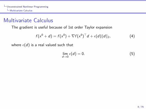
Example (The ε(d) function)
If f (x) = ‖x‖22 and f (x) = x>Ax , where A = A>, what is ε(d)?
Name three functions ε such that limd→0 ε(d) = 0.
Solution:f (x0 + d) = (x0 + d)>A(x0 + d) = x>0 Ax0︸ ︷︷ ︸
=f (x0)
+ 2x>0 A︸ ︷︷ ︸=∇f (x0)>
d + d>Ad
Thus ε(d)‖d‖2 = d>Ad ⇒ ε(d) =d>Ad
‖d‖2and
limd→0
ε(d) = 0
Three examples:
ε(d) = log(d), ε(d) = ‖d‖, ε(d) =a‖d‖3 + b‖d‖2
c‖d‖+ e.
9 / 76

Unconstrained Nonlinear Programming
Multivariate Calculus
The Hessian MatrixIf f ∈ C 2, we refer to ∇2f (x) as the Hessian matrix:
∇2f (x)def=
∂2f (x)∂x1∂x1
∂2f (x)∂x1∂x2
∂2f (x)∂x1∂x3
. . . ∂2f (x)∂x1∂xn
∂2f (x)∂x1∂x2
∂2f (x)∂x2∂x2
∂2f (x)∂x2∂x3
. . . ∂2f (x)∂x2∂xn
......
.... . .
...∂2f (x)∂xn∂x1
∂2f (x)∂xn∂x2
∂2f (x)∂xn∂x3
. . . ∂2f (x)∂xn∂xn
If f ∈ C 2 then
∂2f (x)
∂xi∂xj=∂2f (x)
∂xj∂xi, ∀i , j ∈ {1, . . . , n}, ⇔ ∇2f (x) = ∇2f (x)>.
Hessian matrix useful for 2nd order Taylor expansion.
f (x0 + d) = f (x0) +∇f (x0)>d +1
2d>∇2f (x0)d + ε(d)‖d‖2
2. (7)
Exe: If f (x) = x3 or f (x) = x>Ax what is ε(d)?
Sol: (x + d)3 = x3 + 3x2d + 3xd2 + d3. Thus ε(d) = d
10 / 76

Unconstrained Nonlinear Programming
Multivariate Calculus
The Hessian MatrixIf f ∈ C 2, we refer to ∇2f (x) as the Hessian matrix:
∇2f (x)def=
∂2f (x)∂x1∂x1
∂2f (x)∂x1∂x2
∂2f (x)∂x1∂x3
. . . ∂2f (x)∂x1∂xn
∂2f (x)∂x1∂x2
∂2f (x)∂x2∂x2
∂2f (x)∂x2∂x3
. . . ∂2f (x)∂x2∂xn
......
.... . .
...∂2f (x)∂xn∂x1
∂2f (x)∂xn∂x2
∂2f (x)∂xn∂x3
. . . ∂2f (x)∂xn∂xn
If f ∈ C 2 then
∂2f (x)
∂xi∂xj=∂2f (x)
∂xj∂xi, ∀i , j ∈ {1, . . . , n}, ⇔ ∇2f (x) = ∇2f (x)>.
Hessian matrix useful for 2nd order Taylor expansion.
f (x0 + d) = f (x0) +∇f (x0)>d +1
2d>∇2f (x0)d + ε(d)‖d‖2
2. (7)
Exe: If f (x) = x3 or f (x) = x>Ax what is ε(d)?Sol: (x + d)3 = x3 + 3x2d + 3xd2 + d3. Thus ε(d) = d
10 / 76

Unconstrained Nonlinear Programming
Multivariate Calculus
The Product-ruleThe vector valued version of the product ruleI For any function F (x) : Rn → Rn and matrix A ∈ Rn×n we
have∇(F (x)>A) = ∇F (x)>A. (8)
I For any two vector valued functions F1 and F2 we have that
∇(F1(x)>F2(x)) = ∇F1(x)F2(x) +∇F2(x)F1(x). (9)
Example
Let f (x) = 12x>Ax , where A ∈ Rn×n is a symmetric positive
definite matrix. Calculate the gradient and the Hessian of f (x).
Let F1(x) = A>x and F2(x) = x then∇f (x) = 1
2∇(A>x)x + 12∇(x)A>x = 1
2 (A + A>)x = Ax since∇(A>x) = A>∇(x) = A. Differentiating again∇(∇f (x)) = ∇(Ax) = ∇(A)x +∇(x)A = A.
11 / 76

Unconstrained Nonlinear Programming
Multivariate Calculus
The Product-ruleThe vector valued version of the product ruleI For any function F (x) : Rn → Rn and matrix A ∈ Rn×n we
have∇(F (x)>A) = ∇F (x)>A. (8)
I For any two vector valued functions F1 and F2 we have that
∇(F1(x)>F2(x)) = ∇F1(x)F2(x) +∇F2(x)F1(x). (9)
Example
Let f (x) = 12x>Ax , where A ∈ Rn×n is a symmetric positive
definite matrix. Calculate the gradient and the Hessian of f (x).
Let F1(x) = A>x and F2(x) = x then∇f (x) = 1
2∇(A>x)x + 12∇(x)A>x = 1
2 (A + A>)x = Ax since∇(A>x) = A>∇(x) = A. Differentiating again∇(∇f (x)) = ∇(Ax) = ∇(A)x +∇(x)A = A. 11 / 76

Unconstrained Nonlinear Programming
Local Descent Lemma and Local Optimality
Template method
xk+1 = xk + skdk ,
where sk > 0 is a step size and dk ∈ Rn is search direction. Satisfythe descent condition
f (xk+1) < f (xk).
How to choose d?
12 / 76

Unconstrained Nonlinear Programming
Local Descent Lemma and Local Optimality
How to find d ∈ Rn such that
f (xk + skd) ≤ f (xk).
Lemma (Steepest Descent)
For d ∈ Rn the local change of f (x) around x0 is
∆(d)def= lim
s→0+
f (x0 + sd)− f (x0)
s. (10)
Let v = − ∇f (x0)/‖∇f (x0)‖2 be the normalized gradient. We
have
v = arg mind∈Rn
∆(d)
subject to ‖d‖2 = 1. (11)
The negative normalized gradient is the direction that minimizesthe local change of f (x) around x0. The normalized gradientmaximizes the local change.
13 / 76

Unconstrained Nonlinear Programming
Local Descent Lemma and Local Optimality
Proof.Using 1st order Taylor we have that
f (x0 + sd)− f (x0) = s∇f (x0)>d + ε(sd)s.
Dividing by s and taking the limit s → 0 we have
∆(d) = lims→0+
f (x0 + sd)− f (x0)
s= ∇f (x0)>d+ lim
s→0+ε(sd) = ∇f (x0)>d .
Now using that ‖d‖2 = 1 together with the Cauchy inequality
− ‖∇f (x0)‖2 ≤ ∆(d) = ∇f (x0)>d ≤ ‖∇f (x0)‖2. (12)
The upper and lower bound is achieved when d = ∇f (x0)/‖∇f (x0)‖2
and d = − ∇f (x0)/‖∇f (x0)‖2, respectively.
14 / 76

Unconstrained Nonlinear Programming
Local Descent Lemma and Local Optimality
The search direction d is a descent direction if it has an obtuseangle with the gradient
Corollary (Descent Condition)
If d>∇f (x0) < 0 then there exists s > 0 such that
f (x0 + sd) < f (x0).
Proof.
From (12) we have that ∆(d) = ∇f (x0)>d < 0.Let c = −∇f (x0)>d > 0.Let s > 0 be such that ε(sd) < c
2 . (Because lims→0 ε(sd) = 0 )Consequently from 1st order Taylor:
f (x0 + sd)− f (x0)
s= ∇f (x0)>d + ε(sd) ≤ −c
2< 0.
Re-arranging f (x0 + sd) ≤ f (x0)− s c2 < f (x0)
15 / 76

Unconstrained Nonlinear Programming
Local Descent Lemma and Local Optimality
The search direction d is a descent direction if it has an obtuseangle with the gradient
Corollary (Descent Condition)
If d>∇f (x0) < 0 then there exists s > 0 such that
f (x0 + sd) < f (x0).
Proof.
From (12) we have that ∆(d) = ∇f (x0)>d < 0.Let c = −∇f (x0)>d > 0.
Let s > 0 be such that ε(sd) < c2 . (Because lims→0 ε(sd) = 0 )
Consequently from 1st order Taylor:
f (x0 + sd)− f (x0)
s= ∇f (x0)>d + ε(sd) ≤ −c
2< 0.
Re-arranging f (x0 + sd) ≤ f (x0)− s c2 < f (x0)
15 / 76

Unconstrained Nonlinear Programming
Local Descent Lemma and Local Optimality
The search direction d is a descent direction if it has an obtuseangle with the gradient
Corollary (Descent Condition)
If d>∇f (x0) < 0 then there exists s > 0 such that
f (x0 + sd) < f (x0).
Proof.
From (12) we have that ∆(d) = ∇f (x0)>d < 0.Let c = −∇f (x0)>d > 0.Let s > 0 be such that ε(sd) < c
2 . (Because lims→0 ε(sd) = 0 )
Consequently from 1st order Taylor:
f (x0 + sd)− f (x0)
s= ∇f (x0)>d + ε(sd) ≤ −c
2< 0.
Re-arranging f (x0 + sd) ≤ f (x0)− s c2 < f (x0)
15 / 76

Unconstrained Nonlinear Programming
Local Descent Lemma and Local Optimality
The search direction d is a descent direction if it has an obtuseangle with the gradient
Corollary (Descent Condition)
If d>∇f (x0) < 0 then there exists s > 0 such that
f (x0 + sd) < f (x0).
Proof.
From (12) we have that ∆(d) = ∇f (x0)>d < 0.Let c = −∇f (x0)>d > 0.Let s > 0 be such that ε(sd) < c
2 . (Because lims→0 ε(sd) = 0 )Consequently from 1st order Taylor:
f (x0 + sd)− f (x0)
s= ∇f (x0)>d + ε(sd) ≤ −c
2< 0.
Re-arranging f (x0 + sd) ≤ f (x0)− s c2 < f (x0)
15 / 76

Unconstrained Nonlinear Programming
Sufficient and Necessary conditions for local optimality
Definition of Local Minima
The point x∗ ∈ Rn is a local minima of f (x) if there exists r > 0such that
f (x∗) ≤ f (x), ∀‖x − x∗‖2 < r . (13)
Theorem (Necessary optimality conditions)
If x∗ is a local minima of f (x) then
1 ∇f (x∗) = 0
2 d>∇2f (x∗)d ≥ 0, ∀d ∈ Rn.
So it is necessary that ∇f (x∗) = 0 and the d is positive curvaturedirection before we stop.
16 / 76

Unconstrained Nonlinear Programming
Sufficient and Necessary conditions for local optimality
Proof.
That ∇f (x∗) = 0 follows from Descent Condition. Suppose there existsd ∈ Rn such that d>∇2f (x∗)d < 0. Suppose w.l.o.g that ‖d‖2 = 1.Using the 2nd order Taylor we have that
f (x∗ + sd) = f (x∗) +s2
2d>∇2f (x∗)d + ε(sd)s2.
Let δ > 0 be such that for s ≤ δ we have that ε(sd) < |d>∇2f (x∗)d |/
4.Dividing the above by s2, for s ≤ δ we have that
f (x∗ + sd)
s2=
f (x∗)
s2+
1
2d>∇2f (x∗)d + ε(sd)
<f (x∗)
s2+
1
4d>∇2f (x∗)d ,
thus f (x∗ + sd) < f (x∗) for all s ≤ δ which contradicts the definition oflocal minima.
17 / 76

Unconstrained Nonlinear Programming
Sufficient and Necessary conditions for local optimality
With a slight modification, same conditions they are also sufficient.
Theorem (Sufficient Local Optimality conditions)
If x∗ ∈ Rn is such that
1 ∇f (x∗) = 0
2 d>∇2f (x∗)d > 0, ∀d ∈ Rn with d 6= 0,
then x∗ is a local minima.
We can use this theorem to find local minima!
18 / 76

Unconstrained Nonlinear Programming
Sufficient and Necessary conditions for local optimality
Proof: Let d ∈ Rn. Because ∇2f (x∗) is positive definite, the smallestnon-zero eigenvalue must be strictly positive. Consequently
‖d‖2λmin(∇2f (x∗)) ≤ d>∇2f (x∗)d .
Using the second-order Taylor expansion, we have that
f (x∗ + d) = f (x∗) +1
2d>∇2f (x∗)d + ε(d)‖d‖2
2
≥ f (x∗) +‖d‖2
2
2λmin(∇2f (x∗)) + ε(d)‖d‖2
2.
Let r > 0 be such that every d with ‖d‖ ≤ r we have that
|ε(d)| < λmin(∇2f (x∗))/4 ⇒ ε(d) > −λmin(∇2f (x∗))/4.
Thus for ‖d‖ ≤ r we have
f (x∗ + d) ≥ f (x∗) +‖d‖2
2
2λmin(∇2f (x∗)) + ε(d)‖d‖2
2
≥ f (x∗) +‖d‖2
2
4λmin(∇2f (x∗)) > f (x∗).
19 / 76

Unconstrained Nonlinear Programming
Sufficient and Necessary conditions for local optimality
Exercise
Let f (x) = 12x>Ax − x>b + c , with A symmetric positive definite.
How many local/global minimas can f (x) have? Find a formula forthe minima using only the data A and b.
Proof.
By the sufficient conditions x∗ is a local minima if
∇f (x∗) = 0 ⇔ Ax∗ = b,
and∇2f (x∗) = A � 0.
Since Ax = b has only one solution there exists only one localminima which must be the global minima.
20 / 76

Unconstrained Nonlinear Programming
Convex functions
Convex Functions
f (tx + (1− t)y) ≤ tf (x) + (1− t)f (y), ∀x , y ∈ Rd , t ∈ [0, 1].
21 / 76

Unconstrained Nonlinear Programming
Convex functions
Theorem
If f is a convex function, then every local minima of f is also aglobal minima. We only need to check 1st order ∇f (x∗) = 0!
Proof.Let x∗ be a local minima and suppose there exists x ∈ Rn such thatf (x) < f (x∗). Let zt = tx + (1− t)x∗ for t ∈ [0, 1]. By the definition ofconvexity we have that
f (zt) = f ((1− t)x + tx∗) ≤ (1− t)f (x) + tf (x∗)
< (1− t)f (x∗) + tf (x∗) = f (x∗). (14)
Thus x∗ cannot be a local minima. Indeed, for any r > 0 withr ≤ ‖x − x∗‖2, we have that by choosing t = 1− r/‖x − x∗‖2 we havethat
‖zt − x∗‖2 = (1− t)‖x − x∗‖2 ≤ r .
Yet from (14) we have that f (zt) < f (x∗). A contraction. Thus thereexists no x with f (x) < f (x∗). 22 / 76

Unconstrained Nonlinear Programming
Convex functions
Theorem
If f is twice continuously differentiable, then the following threestatements are equivalent
f (tx + (1− t)y) ≤ tf (x) + (1− t)f (y), ∀x , y , t ∈ [0, 1]. (0th)
f (y) ≥ f (x) +∇f (x)>(y − x), ∀x , y . (1st)
0 ≤ d>∇2f (x)d , ∀x , d . (2nd)
Proof.
We prove (0th)⇒ (1st)⇒ (2nd).The remaing (2nd)⇒ (0th) is left as an exercise.(0th)⇒ (1st): Dividing (0th) by t and re-arranging
f (y + t(x − y))− f (y)
t≤ f (x)− f (y).
Now taking the limit t → 0 gives (1st).23 / 76

Unconstrained Nonlinear Programming
Convex functions
Proof.
(1st)⇒ (2nd): First we prove this holds for 1–dimensional functionsf : R→ R. From (1st) we have that
f (y) ≥ f (x) + f ′(x)(y − x),
f (x) ≥ f (y) + f ′(y)(x − y).
Combining the above two we have that
f ′(x)(y − x) ≤ f (y)− f (x) ≤ f ′(y)(y − x).
Dividing by (y − x)2 we have
f ′(y)− f ′(x)
y − x≥ 0, ∀x , y , x 6= y .
It remains to take the limit. Extend to every n–dimensional functionusing
d2f (x + tv)
dv2
∣∣∣∣t=0
= v>∇2f (x)v ≥ 0,∀v 6= 0.
24 / 76
Unconstrained Nonlinear Programming
Gradient method
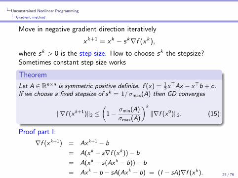
Move in negative gradient direction iteratively
xk+1 = xk − sk∇f (xk),
where sk > 0 is the step size. How to choose sk the stepsize?Sometimes constant step size works
Theorem
Let A ∈ Rn×n is symmetric positive definite. f (x) = 12x>Ax − x>b + c .
If we choose a fixed stepsize of sk = 1/σmax(A) then GD converges
‖∇f (xk+1)‖2 ≤(
1− σmin(A)
σmax(A)
)k
‖∇f (x0)‖2. (15)
Proof part I:
∇f (xk+1) = Axk+1 − b
= A(xk − s∇f (xk))− b
= A(xk − s(Axk − b))− b
= Axk − b − sA(Axk − b) = (I − sA)∇f (xk). 25 / 76

Unconstrained Nonlinear Programming
Gradient method
Proof part II: From ∇f (xk+1) = (I − sA)∇f (xk) taking norms
‖∇f (xk+1)‖2 ≤ ‖I − sA‖2‖∇f (xk)‖2.
Choosing s = 1/σmax(A) we have that I − sA is symmetric positivedefinite and
‖I − sA‖2 = 1− sσmin(A) = 1− σmin(A)
σmax(A)< 1.
Homework: Prove this last step! Thus finally
‖∇f (xk+1)‖2 ≤(
1− σmin(A)
σmax(A)
)‖∇f (xk)‖2
≤(
1− σmin(A)
σmax(A)
)k
‖∇f (x0)‖2.
26 / 76

Unconstrained Nonlinear Programming
Gradient method
What to do for non-quadratic functions? Choose the best sk ?
sk = arg mins≥0
f (xk + sdk).
Seems good, but leads to zig-zagging convergence because
∇f (xk+1)>∇f (xk) = 0.
To prove this
d
dsf (xk − s∇f (xk))
∣∣s=sk
= 0.
Using the chain-rule we have that
d
dsf (xk − s∇f (xk))
∣∣s=sk
= −sk∇f (xk−sk∇f (xk))>∇f (xk) = 0.
27 / 76

Unconstrained Nonlinear Programming
Gradient method
Backtracking Line searchInstead of *best* step size, find a good one.
Algorithm 1 Backtracking Line Search(α, ρ, c)
1: Choose α > 0, ρ, c ∈ (0, 1).2: while f (xk + αdk) ≤ f (xk) + c α∇f (xk)>dk do3: Update α = ρα.
Figure: Where φ(α) = f (xk + αdk) and l(α) = f (xk) + c α∇f (xk)>dk28 / 76

Unconstrained Nonlinear Programming
Gradient method
Putting everything together with a stopping criteria
Algorithm 2 Gradient Descent
1: Choose x0 ∈ Rn.2: while ‖∇f (xk)‖2 > ε or f (xk+1)− f (xk) ≤ ε do3: Calculate dk = −∇f (xk)4: Calculate sk using Backtracking Line Search.5: Update xk+1 = xk + skdk .
Figure: Convergence of Gradient Descent
29 / 76

Unconstrained Nonlinear Programming
Newton’s Method
Gradient uses 1st order approximation. What about 2nd order?
Figure: Comparing 1st order and 2nd Taylor of f (x) = ex .
Local quadratic approximation using 2nd Taylor
qk(x) = f (xk) +∇f (xk)>(x − xk) +1
2(x − xk)>∇2f (xk)(x − xk).
30 / 76

Unconstrained Nonlinear Programming
Newton’s Method
Newton’s Method
Newton’s method minimizes the local quadratic approximation.
qk(x) = f (xk) +∇f (xk)>(x − xk) +1
2(x − xk)>∇2f (xk)(x − xk).
Assume that ∇2f (xk) is invertible. Let xk+1 be the point that solves
∇xqk(x) = ∇f (xk) +∇2f (xk)(xk+1 − xk) = 0.
Isolating xk+1 we have
xk+1 = xk −∇2f (xk)−1∇f (xk) .
Newton’s method can converge at a quadratic speed. Much faster thanGradient Descent.
31 / 76

Unconstrained Nonlinear Programming
Newton’s Method
Theorem
Let f (x) be a µ–strongly convex function:
v>∇2f (x)v ≥ µ‖v‖2, ∀x , v ∈ Rn. (16)
If the Hessian is also Lipschitz
‖∇2f (x)−∇2f (y)‖2 ≤ L‖x − y‖2 (17)
then Newton’s method converges according to
‖xk+1 − x∗‖2 ≤L
2µ‖xk − x∗‖2
2. (18)
In particular if ‖x0 − x∗‖2 ≤ µL , then for k ≥ 1 we have that
‖xk − x∗‖2 ≤1
22k
µ
L. (19)
32 / 76

Unconstrained Nonlinear Programming
Newton’s Method
Proof:
xk+1 − x∗ = xk − x∗ −∇2f (xk)−1(∇f (xk)−∇f (x∗)
)= xk − x∗ −∇2f (xk)−1
∫ 1
s=0
∇2f (xk + s(x∗ − xk))(xk − x∗)ds
= ∇2f (xk)−1
∫ 1
s=0
(∇2f (xk)−∇2f (xk + s(x∗ − xk))
)(xk − x∗)ds
Let δk := xk − x∗. Taking norms we have that
‖δk+1‖ ≤ ‖∇2f (xk)−1‖∫ 1
s=0
‖∇2f (xk)−∇2f (xk + s(x∗ − xk))‖ ‖δk‖ds
≤ L
µ
∫ 1
s=0
s‖δk‖2ds
=L
2µ‖δk‖2.
33 / 76

Unconstrained Nonlinear Programming
Newton’s Method
Proof Part II: So now we have shown
‖xk+1 − x∗‖ ≤ ;L
2µ‖xk − x∗‖2.
If ‖x0 − x∗‖ ≤ µL , then by induction that
‖xk − x∗‖ ≤ 1
22k
µ
L, (20)
then we have that
‖xk+1−x∗‖ ≤ L
2µ‖xk−x∗‖2 ≤ L
2µ
1
22k
1
22k
(µL
)2
<1
22k+1
µ
L,
which concludes the induction proof.
34 / 76

Constrained Nonlinear Optimization
Constrained Nonlinear OptimizationLet f , gi and hj be C 1 continuous functions, for i = 1, . . . ,m andj = 1, . . . , p. Consider the constrained optimization problem
minx∈Rn
f (x)
subject to gi (x) ≤ 0, for i ∈ I .
hj(x) = 0, for j ∈ J, (21)
where I = {1, . . . ,m} and J = {1, . . . , p}. Some notation:
I Inequality constraints: gi (x) ≤ 0, for i ∈ I
I Equality constraints: hj(x) = 0, for j ∈ J
I Feasible point x : Satisfies all inequality and equality constraints.
I Feasible set X : All the feasible points
Xdef= {x ∈ Rn : gi (x) ≤ 0, hj(x) = 0, for i ∈ I , and j ∈ J}.
I Abbreviated form: minx∈X
f (x).
35 / 76

Constrained Nonlinear Optimization
Exercise: Solve the following constrained nonlinear optimization problemgraphically.
minx∈Rn
(x1 − 3)2 + (x2 − 2)2
subject to x21 − x2 − 3 ≤ 0,
x2 − 1 ≤ 0,
−x1 ≤ 0.
Figure: Plot of feasible set
36 / 76

Constrained Nonlinear Optimization
Exercise: Solve the following constrained nonlinear optimization problemgraphically.
minx∈Rn
(x1 − 3)2 + (x2 − 2)2
subject to x21 − x2 − 3 ≤ 0,
x2 − 1 ≤ 0,
−x1 ≤ 0.
Figure: Plot of feasible set
37 / 76

Constrained Nonlinear Optimization
Adding constraints can make the problem easy.Easy example: If X = {x0} is a single point, we are done. IfX = {x0 + td0, ∀t ∈ R} it is easier.But constraints can also make the problem harder (speciallyconceptually). Also even if gi and hj are smooth, the feasible set can benon-smooth. Hard example:
Figure: Difficult feasible set with objective function
38 / 76

Constrained Nonlinear Optimization
Existence Theory
Theorem (Existence)
If the feasible set X is bounded and non-empty, then there exists asolution to minx∈X f (x).
Proof.
Given that the sets R− = [−∞, 0] and {0} are closed, by thecontinuity of gi and hj we have that X is closed. Indeed,
X =
(m⋂i=1
g−1i ([−∞, 0])
)∩
p⋂j=1
h−1j ({0})
,
and thus is a finite intersection of closed sets. By assumption X isbounded, thus it is compact. By the continuity of f we have thatf (X ) is also compact (The Extreme value theorem). Consequentlythere exists a minimum in f (X ).
39 / 76

Constrained Nonlinear Optimization
Existence Theory
Definition
We say that f : Rn → R is coercive if lim‖x‖→∞ f (x) =∞.
Theorem
If X is non-empty and f is coercive, then there exists a solution tominx∈X f (x).
Proof.
Let x0 ∈ X . Define Br := {x : ‖x‖ ≤ r}. Since f is coercive, there existsr such that for each x with ‖x‖ ≥ r we have that f (xk) ≥ f (x0).Otherwise we would be able to construct a sequence xk with ‖xk‖ → ∞such that f (x) ≤ f (x0), which contracts the coercivity of f .Thus clearly the minimum of f is in Br . Since Br is bounded and closed,we have that x0 ∈ Br ∩ X thus it is bounded, closed and nonempty.Again by the extreme value theorem, f (x) attains its minimum in Br ∩X ,which is also the minimum in X .
40 / 76

Constrained Nonlinear Optimization
Admissable and Feasible directions
Given x0 ∈ X how can me move and still stay inside X?If X was a polyhedra then d is a feasible or an admissible direction atx0 ∈ X if there exists ε > 0 such that x0 + td ∈ X for all 0 ≤ t ≤ ε.
Figure: Difficult feasible set with objective function
For the case that the frontier of the feasible set is nonlinear, we need toconsider a more general notion of feasible directions.
41 / 76

Constrained Nonlinear Optimization
Admissable and Feasible directions
Definition
We say that d is an admissible direction at x0 ∈ X if there exists a C 1
differentiable curve φ : R+ → Rn such that
1 φ(0) = x0
2 φ′(0) = d
3 There exists ε > 0 such that t ≤ ε we have φ(t) ∈ X
We denote by A(x0) the set of admissable directions at x0.
Some examples of admissable sets
I As a straight forward example, given d ∈ Rn letX = {x | ∀α ∈ R, x = αd}. For any x0 ∈ X we have thatA(x0) = X .
I Consider the circle X = {(cos(θ), sin(θ)) | 0 ≤ θ ≤ 2π} ⊂ R2. Thenfor every x0 = ((cos(θ0), sin(θ0))) we have that
A(x0) = {(−α sin(θ), α cos(θ)),∀α ∈ R}.42 / 76

Constrained Nonlinear Optimization
Admissable and Feasible directions
Taylor for Composition with Curve
Lemma
Let φ : R+ → Rn be a C 1 curve as defined in Definition 15. Letf : Rn → R be continuously differentiable. Then the first order Taylorexpansion of the composition f (φ(t)) around x0 can be written as
f (φ(t)) = f (x0) + td>∇f (x0) + t ε(t), (22)
where limt→0 ε(t) = 0.
Proof: Since both f and φ are C 1, their composition is also C 1. Thusf (φ(t)) first order Taylor expansion around t = 0 gives
f (φ(t)) = f (φ(0)) + tdf (φ(t))
dt|t=0 + tε(t).
Now plugging in φ(0) = x0 and using the chain-rule
df (φ(t))
dt|t=0 = (φ′(t)>∇f (φ(t)))|t=0 = (d>∇f (x0)).
43 / 76

Constrained Nonlinear Optimization
Admissable and Feasible directions
Theorem (Necessary Condition for Admissable Direction)
Let I0(x0) = {i : gi (x0) = 0, i ∈ I} be the indexes of saturatedinequalities. If d ∈ A(x0) is an admissable direction then
1 For every i ∈ I (x0) we have that d>∇gi (x0) ≤ 0.
2 For every j ∈ J we have that d>∇hj(x0) = 0.
Let B(x0) be the set of directions that satisfy the above two conditions.Thus A(x0) ⊂ B(x0).
Proof 1. Let i ∈ I (x0). Let φ(t) be the curve associated to d . The 1storder Taylor expansion of gi around x0 in the d direction which is
gi (φ(t))(22)= gi (x0) + td>∇gi (x0) + tε(t)
= td>∇gi (x0) + tε(t) ≤ 0,
where we used gi (φ(t)) ≤ 0 for t sufficiently small. Dividing by t gives
d>∇gi (x0) + ε(t) ≤ 0.
Letting t → 0 we have that d>∇gi (x0) ≤ 0. 44 / 76

Constrained Nonlinear Optimization
Admissable and Feasible directions
Theorem (Necessary Condition for Admissable Direction)
Let I0(x0) = {i : gi (x0) = 0, i ∈ I} be the indexes of saturatedinequalities. If d ∈ A(x0) is an admissable direction then
1 For every i ∈ I (x0) we have that d>∇gi (x0) ≤ 0.
2 For every j ∈ J we have that d>∇hj(x0) = 0.
Let B(x0) be the set of directions that satisfy the above two conditions.Thus A(x0) ⊂ B(x0).
Proof 2. Using the first order Taylor expansion of hj around x0 gives
hj(φ(t))(22)= hj(x0) + td>∇hj(x0) + tε(t) = td>∇hj(x0) + tε(t) = 0.
Dividing by t and then taking the limit as t → 0 givesd>∇hj(x0) = 0.
45 / 76

Constrained Nonlinear Optimization
Admissable and Feasible directions
Cone of Feasible DirectionsWe refer to B(x0) as the cone of feasible directions.Cones are easy to work with. We would like to use B(x0) instead A(x0).But sometimes B(x0) and to A(x0) are not the same.
Example (Degeneracy)
Consider the constraint given by
h1(x) = (x21 + x2
2 − 2)2 = 0.
Thus
∇h1(x) = 2(x21 + x2
2 − 2)
(x1
x2
).
Every feasible point satisfies ∇h1(x) = 0. Consequently B(x) = R2 forevery feasible point. Yet h1(x) = 0 describes a circle, and clearly A(x) isthe tangent line at x . Thus we cannot use ∇h1(x) to describe feasibledirections. We would not have this problem if instead we used instead
h1(x) = (x21 + x2
2 − 2) = 0.46 / 76

Constrained Nonlinear Optimization
Admissable and Feasible directions
To exclude these degeneracies, we impose the Constraint qualifications.
Definition
We say that the constraint qualifications hold at x0 if for every d ∈ B(x0)there exists a sequence (dt)
∞t=1 ∈ A(x0) such that dt → d .
Recall
B(x)def={d | d>∇gi (x) ≤ 0, d>∇hj(x0) = 0, ∀j ∈ J, ∀i ∈ I (x)
}.
Constraint qualifications makes things easier.
Theorem (Necessary conditions)
Let x∗ be a local minimum. If the constraint qualification holds at x∗
then for every d ∈ B(x∗) we have that ∇f (x∗)>d ≥ 0. Every direction inthe feasible cone is not descent directions.
So we can check if x∗ is a local minima by testing the directions in thefeasible cone!
47 / 76

Constrained Nonlinear Optimization
Admissable and Feasible directions
Theorem (Necessary conditions)
Let x∗ be a local minimum. If the constraint qualification holds at x∗
then for every d ∈ B(x∗) we have that ∇f (x∗)>d ≥ 0. Every direction inthe feasible cone is not descent directions.
Proof: Let dk ∈ A(x∗) be a sequence such that dk → d . Let φk be thecurve associated to dk . Using the first order Taylor expansion we have
f (φk(t)) = f (x∗) + t∇f (x∗)>dk + tεk(t).
Since x∗ is a local minima, there exists T for which t ≤ T we have thatf (x∗) ≤ f (φk(t)). Consequently
t∇f (x∗)>dk + tεk(t) = f (φk(t))− f (x∗) ≥ 0, for t ≤ T .
Dividing by t and taking the limit we have
limt→0∇f (x∗)
>dk + εk(t) = ∇f (x∗)>dk ≥ 0.
Taking the limit in k concludes the proof.48 / 76

Constrained Nonlinear Optimization
Equality Constrained Optimization
Consider equality constrained optimization problem
minx∈Rn
f (x)
subject to hj(x) = 0, for j ∈ J (23)
Figure: Graphical solution: Not optimal49 / 76

Constrained Nonlinear Optimization
Equality Constrained Optimization
Consider equality constrained optimization problem
minx∈Rn
f (x)
subject to hj(x) = 0, for j ∈ J (24)
Figure: Graphical solution: Optimal50 / 76

Constrained Nonlinear Optimization
Equality Constrained Optimization
Theorem (Langrange’s Condition)
Let x∗ ∈ X be a local minima and suppose that the constraintqualifications hold at x∗ for (32). It follows that the gradient of theobjective is a linear combination of the gradients of constraints at x∗,that is, there exists µj ∈ R for j ∈ J such that
∇f (x∗) =∑j∈J
µj∇hj(x∗). (25)
Let E = span ({∇h1(x∗), . . . ,∇hp(x∗)}) . Let us re-write∇f (x∗) = y + z where y ∈ E and w ∈ E⊥, thus
−z>∇hj(x∗) = 0, ∀j ∈ J.
Thus by definition −z ∈ B(x∗). Consequently by Necessary Conditionswe have that −z>∇f (x∗) ≥ 0. It follows that
−z>∇f (x∗) = −z>y − ‖z‖22 = −‖z‖2
2 ≥ 0.
Consequently z = 0 and ∇f (x∗) = y ∈ E .51 / 76

Constrained Nonlinear Optimization
Equality Constrained Optimization
Consider equality constrained optimization problem
minx∈Rn
f (x)
subject to hj(x) = 0, for j ∈ J (26)
Figure: Graphical solution two constraints: Optimal
52 / 76

Constrained Nonlinear Optimization
Karush, Kuhn and Tuckers condition
minx∈Rn
f (x)
subject to gi (x) ≤ 0, for i ∈ I .
hj(x) = 0, for j ∈ J, (27)
Theorem (Karush, Kuhn and Tuckers condition)
Let x∗ ∈ X be a local minima and suppose that the constraintqualifications hold at x∗ for (26). It follows that there existsµj ∈ R and λi ∈ R+ for j ∈ J and i ∈ I (x∗) such that
∇f (x∗) =∑j∈J
µj∇hj(x∗)−∑
i∈I (x∗)
λi∇gi (x∗). (28)
For this proof, we need to learn about some geometry of Polyhedra.53 / 76

Constrained Nonlinear Optimization
Karush, Kuhn and Tuckers condition
Theorem (Karush, Kuhn and Tuckers condition)
Let x∗ ∈ X be a local minima and suppose that the constraintqualifications hold at x∗ for (26). It follows that there exists µj ∈ R andλi ∈ R+ for j ∈ J and i ∈ I (x∗) such that
∇f (x∗) =∑j∈J
µj∇hj(x∗)−∑
i∈I (x∗)
λi∇gi (x∗).
Figure: Left: Not optimal. Right: Optimal. 54 / 76

Constrained Nonlinear Optimization
Geometry of Polyhedra
Theorem (Separating Hyperplane theorem)
Let X ,Y ⊂ Rn be two disjoint convex sets. Then there exists ahyperplane defined by v ∈ Rn and β ∈ R such that
〈v , x〉 ≤ β and 〈v , y〉 ≥ β, ∀x ∈ X , ∀y ∈ Y .
Figure: Difficult feasible set with objective function
55 / 76

Constrained Nonlinear Optimization
Geometry of Polyhedra
Theorem (Separating a cone and a point)
Consider a given vector b and the cone
Kdef= {Aλ+ Bµ | ∀λ ≥ 0,∀µ}. (29)
Then either b ∈ K or there exists a vector y such that
〈y , b〉 ≤ 0 and 〈y , k〉 ≥ 0, ∀k ∈ K . (30)
Figure: Difficult feasible set with objective function
56 / 76

Constrained Nonlinear Optimization
Geometry of Polyhedra
Figure: Separating a cone and a line
Proof: Let `b = {αb | ∀α > 0} Since K is a cone,
b ∈ K ⇔ K ∩ `b = 6 ∅.Since K and `b are convex sets, by the Separating Hyperplane theoremthere exists a hyperplane separating K and `b. Clearly this hyperplanemust pass through the origin. 57 / 76

Constrained Nonlinear Optimization
Geometry of Polyhedra
Theorem (2nd Version of Farkas Lemma)
Consider the set
P = {(λ, µ) : Aλ+ Bµ = b, λ ≥ 0}
andQ = {y : A>y ≥ 0, B>y = 0}.
The set P is non-empty if and only if every y ∈ Q is such that b>y ≥ 0.
LetK
def= {Aλ+ Bµ | ∀λ ≥ 0,∀µ}.
If P is not empty then b ∈ K .
58 / 76

Constrained Nonlinear Optimization
KKT proof and examples
Proof.If b ∈ P is equivalent to b ∈ K . If b is not in K then there exists aseparating hyperplane that passes through the origin parametrized by avector y . Consequently
〈y ,Aλ+ Bµ〉 = 〈A>y , λ〉+ 〈B>y , µ〉 ≥ 0, ∀λ ≥ 0, ∀µ. (31)
Since this has to hold for every vector µ it is easy to see that B>y = 0.Otherwise, fix λ = 0. If the ith row of B>y is non-zero we can chooseµ = ei and then µ = −ei which when inserted into (31) gives
〈B>y , ei 〉 ≥ 0 and 〈B>y , ei 〉 ≤ 0,
which gives a contradiction and shows that B>y = 0.Furthermore A>y ≥ 0. This follows by simply choosing λ as the ithcoordinate vector. The converse is also true, since if A>y ≥ 0 and λ ≥ 0then clearly their inner product is positive. Finally, from (30) we alsohave that b>y ≥ 0.
59 / 76

Constrained Nonlinear Optimization
KKT proof and examples
minx∈Rn
f (x)
subject to gi (x) ≤ 0, for i ∈ I .
hj(x) = 0, for j ∈ J, (32)
Theorem (Karush, Kuhn and Tuckers condition)
Let x∗ ∈ X be a local minima and suppose that the constraintqualifications hold at x∗ for (26). It follows that there existsµj ∈ R and λi ∈ R+ for j ∈ J and i ∈ I (x∗) such that
∇f (x∗) =∑j∈J
µj∇hj(x∗)−∑
i∈I (x∗)
λi∇gi (x∗). (33)
We call this the KKT equation.
We now prove this using Farkas Lemma.59 / 76

Constrained Nonlinear Optimization
KKT proof and examples
∇f (x∗) =∑j∈J
µj∇hj(x∗)−∑
i∈I (x∗)
λi∇gi (x∗). (34)
Proof KKT: Since Constraint Qualifications holds by the NecessaryConditions Theorem we know that for every d ∈ Rn that satisfies
−d>∇gi (x∗) ≥ 0, for i ∈ I (x∗)
d>∇hj(x∗) = 0, for j ∈ J,
we have that d>∇f (x∗) ≥ 0. By defining b = ∇f (x∗) and
A = [−∇g1(x∗), . . .−∇gm(x∗)] and B = [∇h1(x∗), . . .∇hp(x∗)],
we can re-write the conic constraint as
d ∈ {d : A>d ≥ 0, B>d = 0}
implies that d>b ≥ 0. By Farkas Lemma this is equivalent to there exists(λ, µ) ∈ P where
P = {(λ, µ) : Aλ+ Bµ = b, λ ≥ 0},
which in turn is equivalent to (34).60 / 76

Constrained Nonlinear Optimization
KKT proof and examples
Definition of KKT conditions
There exists x that is feasible x ∈ X and µ ∈ R|J| and λ ∈ R|I | such that:
∇f (x∗) =∑j∈J
µj∇hj(x∗)−∑
i∈I (x∗)
λi∇gi (x∗)
Theorem (Sufficient conditions)
Let f and gi for i ∈ I be convex functions. Let hj be linear for j ∈ J.Suppose the constraint qualifications hold at x∗ ∈ X and the KKTconditions are verified. Then x∗ is a local minima
61 / 76

Constrained Nonlinear Optimization
KKT proof and examples
Proof: Let µj ∈ R and λi ∈ R+ for j ∈ J and i ∈ I (x∗) such thatKKT (33) holds. Let x ∈ X . Since f (x) is convex, we have that
f (x) ≥ f (x∗) +∇f (x∗)>(x − x∗)
(33)= f (x∗) +
∑j∈J
µj∇hj(x∗)>(x − x∗)−∑
i∈I (x∗)
λi∇gi (x∗)>(x − x∗).
Since hj is linear and hj(x) = 0 = hj(x∗) we have that
∇hj(x∗)>(x − x∗) = hj(x)− hj(x∗) = 0.
Since each gi is convex, we have that
∇gi (x∗)>(x − x∗) ≤ gi (x)− gi (x∗)
i∈I (x∗)= gi (x) ≤ 0.
Plugging the above into (35) gives
f (x)(35)
≥ f (x∗)−∑
i∈I (x∗)
λi∇gi (x∗)>(x − x∗).
(35)
≥ f (x∗)−∑
i∈I (x∗)
λigi (x) ≥ f (x∗).
62 / 76

Constrained Nonlinear Optimization
KKT proof and examples
Lagrangian FormulationThe KKT conditions are often described with the help of anauxiliary function called the Lagrangian function
L(x , µ, λ)def= f (x)− 〈µ, h(x)〉+ 〈λ, g(x)〉 , (35)
where h(x)def= (hj(x))j∈J and g(x)
def= (gi (x))i∈I for shorthand.
Theorem
Let x ∈ Rn, µ ∈ R|J| and λ ∈ R|I |. If
∇xL(x , µ, λ) = 0 (36)
∇µL(x , µ, λ) = 0 (37)
∇λL(x , µ, λ) ≤ 0 (38)
then the KKT conditions holds.
63 / 76

Constrained Nonlinear Optimization
KKT proof and examples
Theorem
Let x ∈ Rn, µ ∈ R|J| and λ ∈ R|I |. If
∇xL(x , µ, λ) = 0 (39)
∇µL(x , µ, λ) = 0 (40)
∇λL(x , µ, λ) ≤ 0 (41)
then the KKT conditions holds.
Proof: Differentiating we have that
∇xL(x , µ, λ) = ∇f (x∗)−∑j∈J
µj∇hj(x∗) +∑
i∈I (x∗)
λi∇gi (x∗) (42)
∇µL(x , µ, λ) = h(x) (43)
∇λL(x , µ, λ) = g(x) (44)
Setting (42) to zero is equivalent to (33). Setting (43) to zero andrestricting (44) to be less then zero gives h(x) = 0 and g(x) ≤ x andthus x is feasible, and the KKT conditons hold.
64 / 76

Constrained Nonlinear Optimization
KKT proof and examples
Example: Largest Circle in Ellipse?
min−x2 − y2 =: f (x , y)
subject to ax2 + by2 ≤ 1,
where a > b > 0. Use graphic solution first.
Figure: Graphic solution
65 / 76

Constrained Nonlinear Optimization
KKT proof and examples
Example: Largest Circle in Ellipse?
min−x2 − y2 =: f (x , y)
subject to ax2 + by2 ≤ 1,
where a > b > 0. Use graphic solution first.
Figure: Graphic solution
65 / 76

Constrained Nonlinear Optimization
KKT proof and examples
Solve using the KKT conditions.
min−x2 − y2 =: f (x , y)
subject to ax2 + by2 ≤ 1,
where a > b > 0. Assume that constraint qualifications hold.
Assuming the constraint is active (why?), we have the KKT conditions
2x = 2aλx
2y = 2bλy .
ax2 + by2 = 1. (KKT)
1 x 6= 0. From the KKT we have that 1 = aλ and consequentlyλ = a−1. From 2y = 2bλy , since bλ 6= 1 we have that y = 0. Thefeasibility constraint now gives us that x = ±a−1/2.
2 x = 0. If y 6= 0, then necessarily λ = b−1, and feasibility gives usthat y = ±b−1/2.
In case (1) we have that f (x , y) = −x2 − y2 = −a−1. In case (2) wehave f (x , y) = −b−1. Since −b−1 < −a−1 ≤ 0, we have that(x , y) = (0,±b−1/2) are the two minimum. What is the maximum?
66 / 76

Constrained Nonlinear Optimization
KKT proof and examples
Solve using the KKT conditions.
min−x2 − y2 =: f (x , y)
subject to ax2 + by2 ≤ 1,
where a > b > 0. Assume that constraint qualifications hold.Assuming the constraint is active (why?), we have the KKT conditions
2x = 2aλx
2y = 2bλy .
ax2 + by2 = 1. (KKT)
1 x 6= 0. From the KKT we have that 1 = aλ and consequentlyλ = a−1. From 2y = 2bλy , since bλ 6= 1 we have that y = 0. Thefeasibility constraint now gives us that x = ±a−1/2.
2 x = 0. If y 6= 0, then necessarily λ = b−1, and feasibility gives usthat y = ±b−1/2.
In case (1) we have that f (x , y) = −x2 − y2 = −a−1. In case (2) wehave f (x , y) = −b−1. Since −b−1 < −a−1 ≤ 0, we have that(x , y) = (0,±b−1/2) are the two minimum. What is the maximum? 66 / 76

Constrained Nonlinear Optimization
KKT proof and examples
Example: Quadratic with Linear ConstraintsLet A ∈ Rn×n be symmetric positive definite, B ∈ Rn×n be invertible andb, y ∈ Rn. Consider the problem
min 12x>Ax − b>x
subject to Bx = y .
Write the solution x∗ to the above as a function of A,B, b and y .
Using KKT there exists µ ∈ Rn such that
Ax∗ − b = B>µ
Bx∗ = y
Rearranging gives (A −B>B 0
)(x∗
µ
)=
(by
)Thus (
x∗
µ
)=
(A −B>B 0
)−1(by
).
67 / 76

Constrained Nonlinear Optimization
KKT proof and examples
Example: Quadratic with Linear ConstraintsLet A ∈ Rn×n be symmetric positive definite, B ∈ Rn×n be invertible andb, y ∈ Rn. Consider the problem
min 12x>Ax − b>x
subject to Bx = y .
Write the solution x∗ to the above as a function of A,B, b and y .Using KKT there exists µ ∈ Rn such that
Ax∗ − b = B>µ
Bx∗ = y
Rearranging gives (A −B>B 0
)(x∗
µ
)=
(by
)Thus (
x∗
µ
)=
(A −B>B 0
)−1(by
).
67 / 76

Constrained Nonlinear Optimization
KKT proof and examples
Exercise: Deducing Duality using KKT
Consider the primal problem
maxx
c>x
subject to Ax = b,
x ≥ 0, (P)
Using the KKT condition show that the dual is given by
minx
b>y
subject to A>y ≤ c (D)
68 / 76

Constrained Nonlinear Optimization
KKT proof and examples
In primal change the min for a max, then KKT equations with λ ≥ 0 forthe inequalities and y variables is
A>y + λ = c Colinear gradients
Ax = b Enforcing equality constraints
x ≥ 0 Enforcing inequality constraints
λ ≥ 0 Positive Lagrange multipliers
xiλi = 0, i = 1, . . . , n. Testing if xi is active (45)
The constraint xiλi = 0 checks if the xi ≥ 0 constraint is active or not.Since both x and λ are positive we can rewrite (45) as x>λ ≥ 0.
TheKKT equations of dual with x ≥ 0 Lagrange parameters is
Ax = b Colinear gradients
A>y ≤ c Enforcing inequality constraints
x ≥ 0 Positive Lagrange multipliers
x>(A>y − c) = 0, i = 1, . . . , n. Testing if constraints are active (46)
Now rename λ = c − A>y and substitute throughout.
69 / 76

Constrained Nonlinear Optimization
KKT proof and examples
In primal change the min for a max, then KKT equations with λ ≥ 0 forthe inequalities and y variables is
A>y + λ = c Colinear gradients
Ax = b Enforcing equality constraints
x ≥ 0 Enforcing inequality constraints
λ ≥ 0 Positive Lagrange multipliers
xiλi = 0, i = 1, . . . , n. Testing if xi is active (45)
The constraint xiλi = 0 checks if the xi ≥ 0 constraint is active or not.Since both x and λ are positive we can rewrite (45) as x>λ ≥ 0. TheKKT equations of dual with x ≥ 0 Lagrange parameters is
Ax = b Colinear gradients
A>y ≤ c Enforcing inequality constraints
x ≥ 0 Positive Lagrange multipliers
x>(A>y − c) = 0, i = 1, . . . , n. Testing if constraints are active (46)
Now rename λ = c − A>y and substitute throughout.69 / 76

Constrained Nonlinear Optimization
Project Gradient Descent
Now we come back to designing algorithms that fit the format
xk+1 = xk + skdk , (47)
such that f (xk+1) < f (xk) and xk+1 ∈ X .In the constrained setting we have the additional problem of enforcingxk+1 ∈ X .Divide tasks: Take one step to decrease f and another to becomefeasible. For this we need the Projection Operator.
PX (z)def= arg min
1
2‖x − z‖2
subject to x ∈ X .
With the projection operator we can now define the projected gradientdescent method
xk+1 = PX (xk − sk∇f (xk)) .
First, let us study some examples of projections.70 / 76

Constrained Nonlinear Optimization
Project Gradient Descent
Projection onto the sphere
If X = {x : ‖x‖ ≤ r} where r > 0 show that
PX (z) = rz
‖z‖.
Proof. We can solve this project problem
min1
2‖x − z‖2 subject to ‖x‖2 ≤ r2.
Suppose that ‖z‖ ≤ r . Clearly x = z is the solution.Suppose instead ‖z‖ > r . Since {x : ‖x‖ ≤ r} is a closed set, we knowthe projection will be on the boundary ‖x‖ = r . Let h(x) = ‖x‖2 − r2.Using the KKT conditions we have that
∇f (x) = −µ∇h(x) =⇒ (x − z) = −2µx =⇒ x =z
1 + 2λ.
Since ‖x‖ = r we have that
‖z‖1 + 2µ
= r =⇒ 1
1 + 2µ=
r
‖z‖=⇒ x = r
z
‖z‖.
71 / 76

Constrained Nonlinear Optimization
Project Gradient Descent
Projection onto hyperplane
Let A ∈ Rn×n be and invertible matrix and let b ∈ Rn. IfX = {x : Ax = b}. Show that
PX (z) = z − A>(AA>)−1(Az − b).
Proof The Lagrangian function associated to the projection is given by
L(x , µ) =1
2‖x − z‖2 + µ>(Ax − b). (48)
Taking the derivative in x and setting to zero gives
∇xL(x , µ) = x − z + A>µ = 0 ⇔ x = z − A>µ (49)
Now using that Ax = b and left multiplying the above by A gives
b = Ax = Az − AA>µ = 0.
Since A is invertible, isolating µ in the above gives
µ = (AA>)−1(Az − b).
Inserting this value for µ into (49) gives the solution. 72 / 76

Constrained Nonlinear Optimization
Project Gradient Descent
Remark on Pseudoinverse operators
We did not need A to be square or invertible to define the projection ontoAx = b. Indeed, no matter what A is the set {x : Ax = b} is a closedset, and thus there must exist a solution to the projection optimizationproblem. In general, the projection of z onto Ax = b is given by
PX (z) = z − A†(Az − b),
where A† is known as the Moore-Penrose Pseudoinverse. Infact, thepseudoinverse of a matrix can be defined as the operator that gives thissolution!
73 / 76

Constrained Nonlinear Optimization
Project Gradient Descent
Projected GD: The good and the bad
xk+1 = PX (xk − sk∇f (xk)) .
Figure: PGD can zig-zag and beslow
Good: General, can be applied toany closed convex constraint. Easyto implement when PX (x) is knownBad: If PX (x) is not known, can betoo expensive to approximate. Canzig-zag.
74 / 76

Constrained Nonlinear Optimization
The constrained descent method
Consider the problem
minx∈Rn
f (x)
subject to gi (x) ≤ 0, for i ∈ I . (50)
Develop a method the given feasible point xk ∈ Rn finds xk+1 such that
f (xk) ≤ f (xk+1)
and for which gi (xk+1) ≤ 0 for all i ∈ I .
Hint: Look for an admissible directions d ∈ Rn that are also descentdirection. This can be done by solvig LP
minx∈Rn
d>∇f (xk)
subject to d>∇gi (xk) ≤ 0, ∀i ∈ I (xk)
− 1 ≤ d ≤ 1 (LPd)
75 / 76

Constrained Nonlinear Optimization
The constrained descent method
Algorithm 3 Descent Algorithm
1: Choose x0 ∈ X and ε > 0. Set k = 0.2: while KKT(xk) conditions not verified or ‖∇f (xk)‖ > ε do3: Find d by solving (LPd) . Find feasible direction4: Find s ∈ R+ such that f (xk + sd) < f (xk) and xk + sd ∈ X5: xk+1 = xk + sd . Take a step6: k = k + 1
Issues: LPd is expensive to solve, and this only works when g(x) ≤ 0 is aPolyhedra, and is only efficient in R2.
76 / 76