Embed Size (px)
Citation preview

Optimisation et simulation numerique.
Lecture 1
A. d’Aspremont. M2 MathSV: Optimisation et simulation numerique. 1/106
Today
� Convex optimization: introduction
� Course organization and other gory details...
� Convex sets, functions, basic definitions.
A. d’Aspremont. M2 MathSV: Optimisation et simulation numerique. 2/106

Convex Optimization
A. d’Aspremont. M2 MathSV: Optimisation et simulation numerique. 3/106

Convex Optimization
� How do we identify easy and hard problems?
� Convexity: why is it so important?
� Modeling: how do we recognize easy problems in real applications?
� Algorithms: how do we solve these problems in practice?
A. d’Aspremont. M2 MathSV: Optimisation et simulation numerique. 4/106

Least squares (LS)
minimize ‖Ax− b‖22A ∈ Rm×n, b ∈ Rm are parameters; x ∈ Rn is variable
� Complete theory (existence & uniqueness, sensitivity analysis . . . )
� Several algorithms compute (global) solution reliably
� We can solve dense problems with n = 1000 vbles, m = 10000 terms
� By exploiting structure (e.g., sparsity) can solve far larger problems
. . . LS is a (widely used) technology
A. d’Aspremont. M2 MathSV: Optimisation et simulation numerique. 5/106
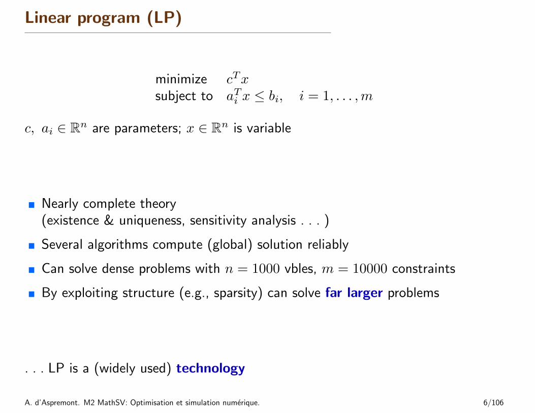
Linear program (LP)
minimize cTxsubject to aTi x ≤ bi, i = 1, . . . ,m
c, ai ∈ Rn are parameters; x ∈ Rn is variable
� Nearly complete theory(existence & uniqueness, sensitivity analysis . . . )
� Several algorithms compute (global) solution reliably
� Can solve dense problems with n = 1000 vbles, m = 10000 constraints
� By exploiting structure (e.g., sparsity) can solve far larger problems
. . . LP is a (widely used) technology
A. d’Aspremont. M2 MathSV: Optimisation et simulation numerique. 6/106

Quadratic program (QP)
minimize ‖Fx− g‖22subject to aTi x ≤ bi, i = 1, . . . ,m
� Combination of LS & LP
� Same story . . . QP is a technology
� Reliability: Programmed on chips to solve real-time problems
� Classic application: portfolio optimization
A. d’Aspremont. M2 MathSV: Optimisation et simulation numerique. 7/106

The bad news
� LS, LP, and QP are exceptions
� Most optimization problems, even some very simple looking ones, areintractable
� The objective of this class is to show you how to recognize the nice ones. . .
� Many, many applications across all fields. . .
A. d’Aspremont. M2 MathSV: Optimisation et simulation numerique. 8/106

Polynomial minimization
minimize p(x)
p is polynomial of degree d; x ∈ Rn is variable
� Except for special cases (e.g., d = 2) this is a very difficult problem
� Even sparse problems with size n = 20, d = 10 are essentially intractable
� All algorithms known to solve this problem require effort exponential in n
A. d’Aspremont. M2 MathSV: Optimisation et simulation numerique. 9/106

What makes a problem easy or hard?
Classical view:
� linear is easy
� nonlinear is hard(er)
A. d’Aspremont. M2 MathSV: Optimisation et simulation numerique. 10/106

What makes a problem easy or hard?
Emerging (and correct) view:
. . . the great watershed in optimization isn’t between linearity andnonlinearity, but convexity and nonconvexity.
— R. Rockafellar, SIAM Review 1993
A. d’Aspremont. M2 MathSV: Optimisation et simulation numerique. 11/106

Convex optimization
minimize f0(x)subject to f1(x) ≤ 0, . . . , fm(x) ≤ 0
x ∈ Rn is optimization variable; fi : Rn → R are convex:
fi(λx+ (1− λ)y) ≤ λfi(x) + (1− λ)fi(y)
for all x, y, 0 ≤ λ ≤ 1
� includes LS, LP, QP, and many others
� like LS, LP, and QP, convex problems are fundamentally tractable
A. d’Aspremont. M2 MathSV: Optimisation et simulation numerique. 12/106

Convex Optimization
A brief history. . .
� The field is about 50 years old.
� Starts with the work of Von Neumann, Kuhn and Tucker, etc
� Explodes in the 60’s with the advent of “relatively” cheap and efficientcomputers. . .
� Key to all this: fast linear algebra
� Some of the theory developed before computers even existed. . .
A. d’Aspremont. M2 MathSV: Optimisation et simulation numerique. 13/106

Convex optimization: history
� Convexity =⇒ low complexity:
”... In fact the great watershed in optimization isn’t between linearity andnonlinearity, but convexity and nonconvexity.” T. Rockafellar.
� True: Nemirovskii and Yudin [1979].
� Very true: Karmarkar [1984].
� Seriously true: convex programming, Nesterov and Nemirovskii [1994].
A. d’Aspremont. M2 MathSV: Optimisation et simulation numerique. 14/106
Standard convex complexity analysis
� All convex minimization problems with: a first order oracle (returning f(x) anda subgradient) can be solved in polynomial time in size and number ofprecision digits.
� Proved using the ellipsoid method by Nemirovskii and Yudin [1979].
� Very slow convergence in practice.
A. d’Aspremont. M2 MathSV: Optimisation et simulation numerique. 15/106

Linear Programming
� Simplex algorithm by Dantzig (1949): exponential worst-case complexity, veryefficient in most cases.
� Khachiyan [1979] then used the ellipsoid method to show the polynomialcomplexity of LP.
� Karmarkar [1984] describes the first efficient polynomial time algorithm for LP,using interior point methods.
A. d’Aspremont. M2 MathSV: Optimisation et simulation numerique. 16/106

From LP to structured convex programs
� Nesterov and Nemirovskii [1994] show that the interior point methods used forLPs can be applied to a larger class of structured convex problems.
� The self-concordance analysis that they introduce extends the polynomialtime complexity proof for LPs.
� Most operations that preserve convexity also preserve self-concordance.
� The complexity of a certain number of elementary problems can be directlyextended to a much wider class.
A. d’Aspremont. M2 MathSV: Optimisation et simulation numerique. 17/106

Symmetric cone programs
� An important particular case: linear programming on symmetric cones
minimize cTxsubject to Ax− b ∈ K
� These include the LP, second-order (Lorentz) and semidefinite cone:
LP: {x ∈ Rn : x ≥ 0}Second order: {(x, y) ∈ Rn × R : ‖x‖ ≤ y}Semidefinite: {X ∈ Sn : X � 0}
� Again, the class of problems that can be represented using these cones isextremely vast.
A. d’Aspremont. M2 MathSV: Optimisation et simulation numerique. 18/106

Course Organization
A. d’Aspremont. M2 MathSV: Optimisation et simulation numerique. 19/106
Course Plan
� Convex analysis & modeling
� Duality
� Algorithms: interior point methods, first order methods.
� Applications
A. d’Aspremont. M2 MathSV: Optimisation et simulation numerique. 20/106

Grading
Course website with lecture notes, homework, etc.
http://www.cmap.polytechnique.fr/~aspremon/MathSVM2.html
� A few homeworks, will be posted online.
� Final exam: TBD
A. d’Aspremont. M2 MathSV: Optimisation et simulation numerique. 21/106

Short blurb
� Contact info on http://www.cmap.polytechnique.fr/~aspremon
� Email: [email protected]
� Dual PhDs: Ecole Polytechnique & Stanford University
� Interests: Optimization, machine learning, statistics & finance.
Recruiting PhD students starting next year. Full ERC funding for 3 years.
A. d’Aspremont. M2 MathSV: Optimisation et simulation numerique. 22/106

References
� All lecture notes will be posted online
� Textbook: Convex Optimization by Lieven Vandenberghe and Stephen Boyd,available online at:
http://www.stanford.edu/~boyd/cvxbook/
� See also Ben-Tal and Nemirovski [2001], “Lectures On Modern ConvexOptimization: Analysis, Algorithms, And Engineering Applications”, SIAM.
http://www2.isye.gatech.edu/~nemirovs/
� Nesterov [2003], “Introductory Lectures on Convex Optimization”, Springer.
� Nesterov and Nemirovskii [1994], “Interior Point Polynomial Algorithms inConvex Programming”, SIAM.
A. d’Aspremont. M2 MathSV: Optimisation et simulation numerique. 23/106

Convex Sets
A. d’Aspremont. M2 MathSV: Optimisation et simulation numerique. 24/106

Convex Sets
� affine and convex sets
� some important examples
� operations that preserve convexity
� generalized inequalities
� separating and supporting hyperplanes
� dual cones and generalized inequalities
A. d’Aspremont. M2 MathSV: Optimisation et simulation numerique. 25/106

Affine set
line through x1, x2: all points
x = θx1 + (1− θ)x2 (θ ∈ R)
x1
x2
θ = 1.2θ = 1
θ = 0.6
θ = 0θ = −0.2
affine set: contains the line through any two distinct points in the set
example: solution set of linear equations {x | Ax = b}
A. d’Aspremont. M2 MathSV: Optimisation et simulation numerique. 26/106

Convex set
line segment between x1 and x2: all points
x = θx1 + (1− θ)x2
with 0 ≤ θ ≤ 1
convex set: contains line segment between any two points in the set
x1, x2 ∈ C, 0 ≤ θ ≤ 1 =⇒ θx1 + (1− θ)x2 ∈ C
examples (one convex, two nonconvex sets)
A. d’Aspremont. M2 MathSV: Optimisation et simulation numerique. 27/106

Convex combination and convex hull
convex combination of x1,. . . , xk: any point x of the form
x = θ1x1 + θ2x2 + · · ·+ θkxk
with θ1 + · · ·+ θk = 1, θi ≥ 0
convex hull CoS: set of all convex combinations of points in S
A. d’Aspremont. M2 MathSV: Optimisation et simulation numerique. 28/106

Convex cone
conic (nonnegative) combination of x1 and x2: any point of the form
x = θ1x1 + θ2x2
with θ1 ≥ 0, θ2 ≥ 0
0
x1
x2
convex cone: set that contains all conic combinations of points in the set
A. d’Aspremont. M2 MathSV: Optimisation et simulation numerique. 29/106

Hyperplanes and halfspaces
hyperplane: set of the form {x | aTx = b} (a 6= 0)
a
x
aTx = b
x0
halfspace: set of the form {x | aTx ≤ b} (a 6= 0)
a
aTx ≥ b
aTx ≤ b
x0
� a is the normal vector
� hyperplanes are affine and convex; halfspaces are convex
A. d’Aspremont. M2 MathSV: Optimisation et simulation numerique. 30/106

Euclidean balls and ellipsoids
(Euclidean) ball with center xc and radius r:
B(xc, r) = {x | ‖x− xc‖2 ≤ r} = {xc + ru | ‖u‖2 ≤ 1}
ellipsoid: set of the form
{x | (x− xc)TP−1(x− xc) ≤ 1}
with P ∈ Sn++ (i.e., P symmetric positive definite)
xc
other representation: {xc +Au | ‖u‖2 ≤ 1} with A square and nonsingular
A. d’Aspremont. M2 MathSV: Optimisation et simulation numerique. 31/106

Norm balls and norm cones
norm: a function ‖ · ‖ that satisfies
� ‖x‖ ≥ 0; ‖x‖ = 0 if and only if x = 0
� ‖tx‖ = |t| ‖x‖ for t ∈ R
� ‖x+ y‖ ≤ ‖x‖+ ‖y‖
notation: ‖ · ‖ is general (unspecified) norm; ‖ · ‖symb is particular norm
norm ball with center xc and radius r: {x | ‖x− xc‖ ≤ r}
norm cone: {(x, t) | ‖x‖ ≤ t}
Euclidean norm cone is called second-order cone
x1x2
t
−1
0
1
−1
0
10
0.5
1
norm balls and cones are convex
A. d’Aspremont. M2 MathSV: Optimisation et simulation numerique. 32/106
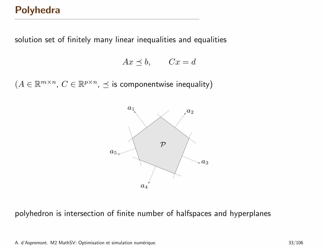
Polyhedra
solution set of finitely many linear inequalities and equalities
Ax � b, Cx = d
(A ∈ Rm×n, C ∈ Rp×n, � is componentwise inequality)
a1 a2
a3
a4
a5
P
polyhedron is intersection of finite number of halfspaces and hyperplanes
A. d’Aspremont. M2 MathSV: Optimisation et simulation numerique. 33/106

Positive semidefinite cone
notation:
� Sn is set of symmetric n× n matrices
� Sn+ = {X ∈ Sn | X � 0}: positive semidefinite n× n matrices
X ∈ Sn+ ⇐⇒ zTXz ≥ 0 for all z
Sn+ is a convex cone
� Sn++ = {X ∈ Sn | X � 0}: positive definite n× n matrices
example:
[x yy z
]∈ S2
+
xy
z
0
0.5
1
−1
0
10
0.5
1
A. d’Aspremont. M2 MathSV: Optimisation et simulation numerique. 34/106

Operations that preserve convexity
practical methods for establishing convexity of a set C
1. apply definition
x1, x2 ∈ C, 0 ≤ θ ≤ 1 =⇒ θx1 + (1− θ)x2 ∈ C
2. show that C is obtained from simple convex sets (hyperplanes, halfspaces,norm balls, . . . ) by operations that preserve convexity
� intersection
� affine functions
� perspective function
� linear-fractional functions
A. d’Aspremont. M2 MathSV: Optimisation et simulation numerique. 35/106

Intersection
the intersection of (any number of) convex sets is convex
example:S = {x ∈ Rm | |p(t)| ≤ 1 for |t| ≤ π/3}
where p(t) = x1 cos t+ x2 cos 2t+ · · ·+ xm cosmt
for m = 2:
0 π/3 2π/3 π
−1
0
1
t
p(t)
x1
x2 S
−2 −1 0 1 2−2
−1
0
1
2
A. d’Aspremont. M2 MathSV: Optimisation et simulation numerique. 36/106

Affine function
suppose f : Rn → Rm is affine (f(x) = Ax+ b with A ∈ Rm×n, b ∈ Rm)
� the image of a convex set under f is convex
S ⊆ Rn convex =⇒ f(S) = {f(x) | x ∈ S} convex
� the inverse image f−1(C) of a convex set under f is convex
C ⊆ Rm convex =⇒ f−1(C) = {x ∈ Rn | f(x) ∈ C} convex
examples
� scaling, translation, projection
� solution set of linear matrix inequality {x | x1A1 + · · ·+ xmAm � B}(with Ai, B ∈ Sp)
� hyperbolic cone {x | xTPx ≤ (cTx)2, cTx ≥ 0} (with P ∈ Sn+)
A. d’Aspremont. M2 MathSV: Optimisation et simulation numerique. 37/106

Perspective and linear-fractional function
perspective function P : Rn+1 → Rn:
P (x, t) = x/t, domP = {(x, t) | t > 0}
images and inverse images of convex sets under perspective are convex
linear-fractional function f : Rn → Rm:
f(x) =Ax+ b
cTx+ d, dom f = {x | cTx+ d > 0}
images and inverse images of convex sets under linear-fractional functions areconvex
A. d’Aspremont. M2 MathSV: Optimisation et simulation numerique. 38/106

example of a linear-fractional function
f(x) =1
x1 + x2 + 1x
x1
x2 C
−1 0 1−1
0
1
x1
x2
f(C)
−1 0 1−1
0
1
A. d’Aspremont. M2 MathSV: Optimisation et simulation numerique. 39/106

Generalized inequalities
a convex cone K ⊆ Rn is a proper cone if
� K is closed (contains its boundary)
� K is solid (has nonempty interior)
� K is pointed (contains no line)
examples
� nonnegative orthant K = Rn+ = {x ∈ Rn | xi ≥ 0, i = 1, . . . , n}
� positive semidefinite cone K = Sn+
� nonnegative polynomials on [0, 1]:
K = {x ∈ Rn | x1 + x2t+ x3t2 + · · ·+ xnt
n−1 ≥ 0 for t ∈ [0, 1]}
A. d’Aspremont. M2 MathSV: Optimisation et simulation numerique. 40/106

generalized inequality defined by a proper cone K:
x �K y ⇐⇒ y − x ∈ K, x ≺K y ⇐⇒ y − x ∈ intK
examples
� componentwise inequality (K = Rn+)
x �Rn+y ⇐⇒ xi ≤ yi, i = 1, . . . , n
� matrix inequality (K = Sn+)
X �Sn+Y ⇐⇒ Y −X positive semidefinite
these two types are so common that we drop the subscript in �K
properties: many properties of �K are similar to ≤ on R, e.g.,
x �K y, u �K v =⇒ x+ u �K y + v
A. d’Aspremont. M2 MathSV: Optimisation et simulation numerique. 41/106

Minimum and minimal elements
�K is not in general a linear ordering : we can have x 6�K y and y 6�K x
x ∈ S is the minimum element of S with respect to �K if
y ∈ S =⇒ x �K y
x ∈ S is a minimal element of S with respect to �K if
y ∈ S, y �K x =⇒ y = x
example (K = R2+)
x1 is the minimum element of S1
x2 is a minimal element of S2 x1
x2S1
S2
A. d’Aspremont. M2 MathSV: Optimisation et simulation numerique. 42/106

Separating hyperplane theorem
if C and D are disjoint convex sets, then there exists a 6= 0, b such that
aTx ≤ b for x ∈ C, aTx ≥ b for x ∈ D
D
C
a
aTx ≥ b aTx ≤ b
the hyperplane {x | aTx = b} separates C and D
strict separation requires additional assumptions (e.g., C is closed, D is asingleton)
A. d’Aspremont. M2 MathSV: Optimisation et simulation numerique. 43/106
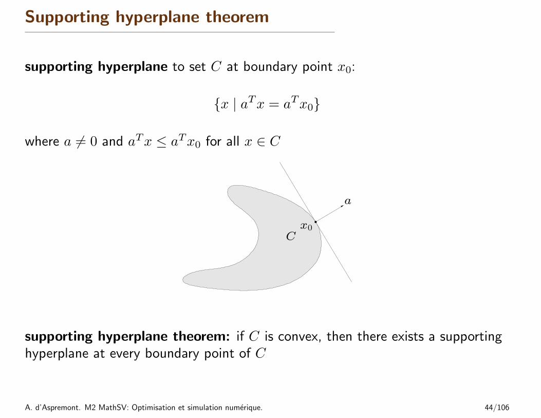
Supporting hyperplane theorem
supporting hyperplane to set C at boundary point x0:
{x | aTx = aTx0}
where a 6= 0 and aTx ≤ aTx0 for all x ∈ C
C
a
x0
supporting hyperplane theorem: if C is convex, then there exists a supportinghyperplane at every boundary point of C
A. d’Aspremont. M2 MathSV: Optimisation et simulation numerique. 44/106

Dual cones and generalized inequalities
dual cone of a cone K:
K∗ = {y | yTx ≥ 0 for all x ∈ K}
examples
� K = Rn+: K∗ = Rn+� K = Sn+: K∗ = Sn+
� K = {(x, t) | ‖x‖2 ≤ t}: K∗ = {(x, t) | ‖x‖2 ≤ t}
� K = {(x, t) | ‖x‖1 ≤ t}: K∗ = {(x, t) | ‖x‖∞ ≤ t}
first three examples are self-dual cones
dual cones of proper cones are proper, hence define generalized inequalities:
y �K∗ 0 ⇐⇒ yTx ≥ 0 for all x �K 0
A. d’Aspremont. M2 MathSV: Optimisation et simulation numerique. 45/106

Minimum and minimal elements via dual inequalities
minimum element w.r.t. �Kx is minimum element of S iff for allλ �K∗ 0, x is the unique minimizer ofλTz over S
x
S
minimal element w.r.t. �K
� if x minimizes λTz over S for some λ �K∗ 0, then x is minimal
Sx1
x2
λ1
λ2
� if x is a minimal element of a convex set S, then there exists a nonzeroλ �K∗ 0 such that x minimizes λTz over S
A. d’Aspremont. M2 MathSV: Optimisation et simulation numerique. 46/106

Convex Functions
A. d’Aspremont. M2 MathSV: Optimisation et simulation numerique. 47/106

Outline
� basic properties and examples
� operations that preserve convexity
� the conjugate function
� quasiconvex functions
� log-concave and log-convex functions
� convexity with respect to generalized inequalities
A. d’Aspremont. M2 MathSV: Optimisation et simulation numerique. 48/106

Definition
f : Rn → R is convex if dom f is a convex set and
f(θx+ (1− θ)y) ≤ θf(x) + (1− θ)f(y)
for all x, y ∈ dom f , 0 ≤ θ ≤ 1
(x, f(x))
(y, f(y))
� f is concave if −f is convex
� f is strictly convex if dom f is convex and
f(θx+ (1− θ)y) < θf(x) + (1− θ)f(y)
for x, y ∈ dom f , x 6= y, 0 < θ < 1
A. d’Aspremont. M2 MathSV: Optimisation et simulation numerique. 49/106

Examples on R
convex:
� affine: ax+ b on R, for any a, b ∈ R
� exponential: eax, for any a ∈ R
� powers: xα on R++, for α ≥ 1 or α ≤ 0
� powers of absolute value: |x|p on R, for p ≥ 1
� negative entropy: x log x on R++
concave:
� affine: ax+ b on R, for any a, b ∈ R
� powers: xα on R++, for 0 ≤ α ≤ 1
� logarithm: log x on R++
A. d’Aspremont. M2 MathSV: Optimisation et simulation numerique. 50/106

Examples on Rn and Rm×n
affine functions are convex and concave; all norms are convex
examples on Rn
� affine function f(x) = aTx+ b
� norms: ‖x‖p = (∑ni=1 |xi|p)1/p for p ≥ 1; ‖x‖∞ = maxk |xk|
examples on Rm×n (m× n matrices)
� affine function
f(X) = Tr(ATX) + b =
m∑i=1
n∑j=1
AijXij + b
� spectral (maximum singular value) norm
f(X) = ‖X‖2 = σmax(X) = (λmax(XTX))1/2
A. d’Aspremont. M2 MathSV: Optimisation et simulation numerique. 51/106

Restriction of a convex function to a line
f : Rn → R is convex if and only if the function g : R→ R,
g(t) = f(x+ tv), dom g = {t | x+ tv ∈ dom f}
is convex (in t) for any x ∈ dom f , v ∈ Rn
can check convexity of f by checking convexity of functions of one variable
example. f : Sn → R with f(X) = log detX, domX = Sn++
g(t) = log det(X + tV ) = log detX + log det(I + tX−1/2V X−1/2)
= log detX +
n∑i=1
log(1 + tλi)
where λi are the eigenvalues of X−1/2V X−1/2
g is concave in t (for any choice of X � 0, V ); hence f is concave
A. d’Aspremont. M2 MathSV: Optimisation et simulation numerique. 52/106

Extended-value extension
extended-value extension f of f is
f(x) = f(x), x ∈ dom f, f(x) =∞, x 6∈ dom f
often simplifies notation; for example, the condition
0 ≤ θ ≤ 1 =⇒ f(θx+ (1− θ)y) ≤ θf(x) + (1− θ)f(y)
(as an inequality in R ∪ {∞}), means the same as the two conditions
� dom f is convex
� for x, y ∈ dom f ,
0 ≤ θ ≤ 1 =⇒ f(θx+ (1− θ)y) ≤ θf(x) + (1− θ)f(y)
A. d’Aspremont. M2 MathSV: Optimisation et simulation numerique. 53/106

First-order condition
f is differentiable if dom f is open and the gradient
∇f(x) =
(∂f(x)
∂x1,∂f(x)
∂x2, . . . ,
∂f(x)
∂xn
)exists at each x ∈ dom f
1st-order condition: differentiable f with convex domain is convex iff
f(y) ≥ f(x) +∇f(x)T (y − x) for all x, y ∈ dom f
(x, f(x))
f(y)
f(x) + ∇f(x)T (y − x)
first-order approximation of f is global underestimator
A. d’Aspremont. M2 MathSV: Optimisation et simulation numerique. 54/106

Second-order conditions
f is twice differentiable if dom f is open and the Hessian ∇2f(x) ∈ Sn,
∇2f(x)ij =∂2f(x)
∂xi∂xj, i, j = 1, . . . , n,
exists at each x ∈ dom f
2nd-order conditions: for twice differentiable f with convex domain
� f is convex if and only if
∇2f(x) � 0 for all x ∈ dom f
� if ∇2f(x) � 0 for all x ∈ dom f , then f is strictly convex
A. d’Aspremont. M2 MathSV: Optimisation et simulation numerique. 55/106

Examples
quadratic function: f(x) = (1/2)xTPx+ qTx+ r (with P ∈ Sn)
∇f(x) = Px+ q, ∇2f(x) = P
convex if P � 0
least-squares objective: f(x) = ‖Ax− b‖22
∇f(x) = 2AT (Ax− b), ∇2f(x) = 2ATA
convex (for any A)
quadratic-over-linear: f(x, y) = x2/y
∇2f(x, y) =2
y3
[y−x
] [y−x
]T� 0
convex for y > 0 xy
f(x
,y)
−2
0
2
0
1
20
1
2
A. d’Aspremont. M2 MathSV: Optimisation et simulation numerique. 56/106

log-sum-exp: f(x) = log∑nk=1 expxk is convex
∇2f(x) =1
1Tzdiag(z)− 1
(1Tz)2zzT (zk = expxk)
to show ∇2f(x) � 0, we must verify that vT∇2f(x)v ≥ 0 for all v:
vT∇2f(x)v =(∑k zkv
2k)(∑k zk)− (
∑k vkzk)
2
(∑k zk)
2≥ 0
since (∑k vkzk)
2 ≤ (∑k zkv
2k)(∑k zk) (from Cauchy-Schwarz inequality)
geometric mean: f(x) = (∏nk=1 xk)
1/n on Rn++ is concave
(similar proof as for log-sum-exp)
A. d’Aspremont. M2 MathSV: Optimisation et simulation numerique. 57/106
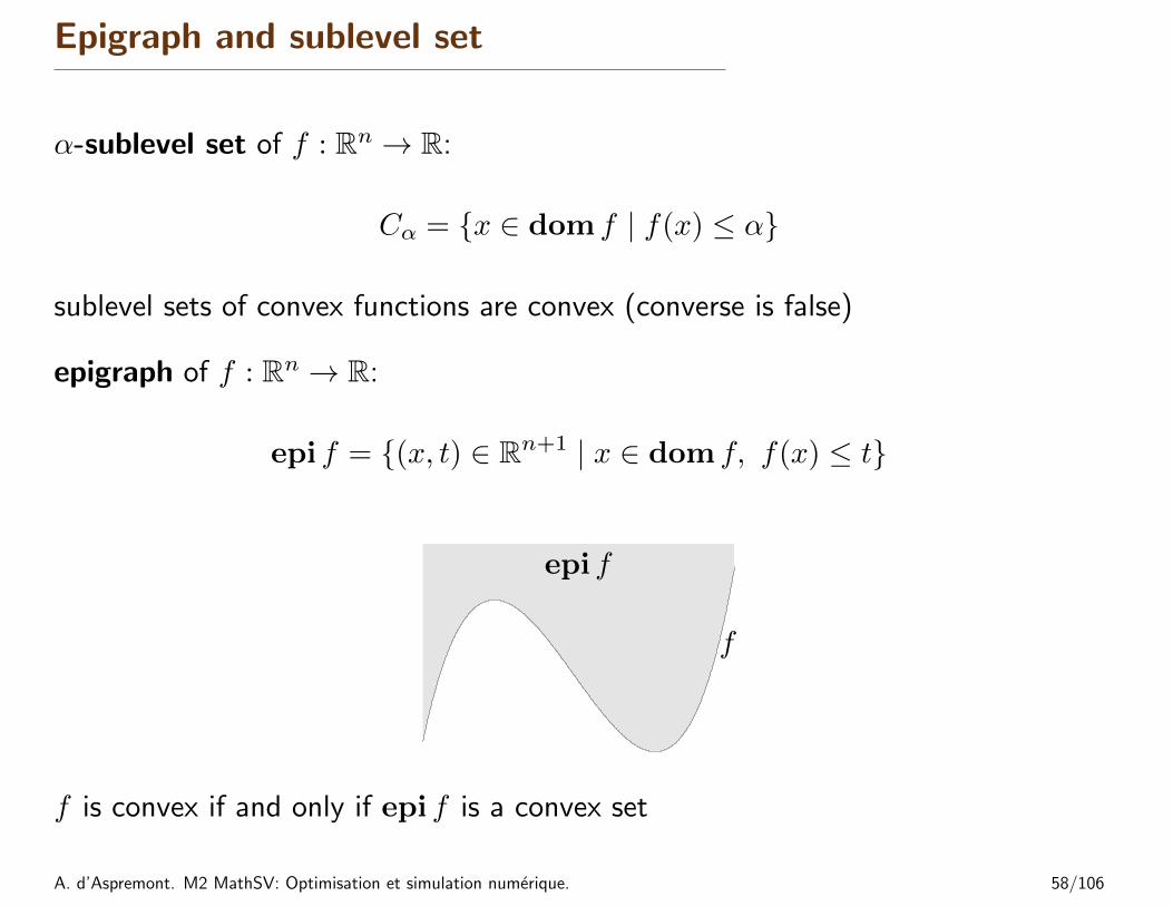
Epigraph and sublevel set
α-sublevel set of f : Rn → R:
Cα = {x ∈ dom f | f(x) ≤ α}
sublevel sets of convex functions are convex (converse is false)
epigraph of f : Rn → R:
epi f = {(x, t) ∈ Rn+1 | x ∈ dom f, f(x) ≤ t}
epi f
f
f is convex if and only if epi f is a convex set
A. d’Aspremont. M2 MathSV: Optimisation et simulation numerique. 58/106
Jensen’s inequality
basic inequality: if f is convex, then for 0 ≤ θ ≤ 1,
f(θx+ (1− θ)y) ≤ θf(x) + (1− θ)f(y)
extension: if f is convex, then
f(E z) ≤ E f(z)
for any random variable z
basic inequality is special case with discrete distribution
Prob(z = x) = θ, Prob(z = y) = 1− θ
A. d’Aspremont. M2 MathSV: Optimisation et simulation numerique. 59/106

Operations that preserve convexity
practical methods for establishing convexity of a function
1. verify definition (often simplified by restricting to a line)
2. for twice differentiable functions, show ∇2f(x) � 0
3. show that f is obtained from simple convex functions by operations thatpreserve convexity
� nonnegative weighted sum� composition with affine function� pointwise maximum and supremum� composition� minimization� perspective
A. d’Aspremont. M2 MathSV: Optimisation et simulation numerique. 60/106

Positive weighted sum & composition with affine function
nonnegative multiple: αf is convex if f is convex, α ≥ 0
sum: f1 + f2 convex if f1, f2 convex (extends to infinite sums, integrals)
composition with affine function: f(Ax+ b) is convex if f is convex
examples
� log barrier for linear inequalities
f(x) = −m∑i=1
log(bi − aTi x), dom f = {x | aTi x < bi, i = 1, . . . ,m}
� (any) norm of affine function: f(x) = ‖Ax+ b‖
A. d’Aspremont. M2 MathSV: Optimisation et simulation numerique. 61/106

Pointwise maximum
if f1, . . . , fm are convex, then f(x) = max{f1(x), . . . , fm(x)} is convex
examples
� piecewise-linear function: f(x) = maxi=1,...,m(aTi x+ bi) is convex
� sum of r largest components of x ∈ Rn:
f(x) = x[1] + x[2] + · · ·+ x[r]
is convex (x[i] is ith largest component of x)
proof:
f(x) = max{xi1 + xi2 + · · ·+ xir | 1 ≤ i1 < i2 < · · · < ir ≤ n}
A. d’Aspremont. M2 MathSV: Optimisation et simulation numerique. 62/106

Pointwise supremum
if f(x, y) is convex in x for each y ∈ A, then
g(x) = supy∈A
f(x, y)
is convex
examples
� support function of a set C: SC(x) = supy∈C yTx is convex
� distance to farthest point in a set C:
f(x) = supy∈C‖x− y‖
� maximum eigenvalue of symmetric matrix: for X ∈ Sn,
λmax(X) = sup‖y‖2=1
yTXy
A. d’Aspremont. M2 MathSV: Optimisation et simulation numerique. 63/106

Composition with scalar functions
composition of g : Rn → R and h : R→ R:
f(x) = h(g(x))
f is convex ifg convex, h convex, h nondecreasing
g concave, h convex, h nonincreasing
� proof (for n = 1, differentiable g, h)
f ′′(x) = h′′(g(x))g′(x)2 + h′(g(x))g′′(x)
� note: monotonicity must hold for extended-value extension h
examples
� exp g(x) is convex if g is convex
� 1/g(x) is convex if g is concave and positive
A. d’Aspremont. M2 MathSV: Optimisation et simulation numerique. 64/106

Vector composition
composition of g : Rn → Rk and h : Rk → R:
f(x) = h(g(x)) = h(g1(x), g2(x), . . . , gk(x))
f is convex ifgi convex, h convex, h nondecreasing in each argument
gi concave, h convex, h nonincreasing in each argument
proof (for n = 1, differentiable g, h)
f ′′(x) = g′(x)T∇2h(g(x))g′(x) +∇h(g(x))Tg′′(x)
examples
�∑mi=1 log gi(x) is concave if gi are concave and positive
� log∑mi=1 exp gi(x) is convex if gi are convex
A. d’Aspremont. M2 MathSV: Optimisation et simulation numerique. 65/106
Minimization
if f(x, y) is convex in (x, y) and C is a convex set, then
g(x) = infy∈C
f(x, y)
is convex
examples
� f(x, y) = xTAx+ 2xTBy + yTCy with[A BBT C
]� 0, C � 0
minimizing over y gives g(x) = infy f(x, y) = xT (A−BC−1BT )x
g is convex, hence Schur complement A−BC−1BT � 0
� distance to a set: dist(x, S) = infy∈S ‖x− y‖ is convex if S is convex
A. d’Aspremont. M2 MathSV: Optimisation et simulation numerique. 66/106

The conjugate function
the conjugate of a function f is
f∗(y) = supx∈dom f
(yTx− f(x))
f(x)
(0,−f∗(y))
xy
x
� f∗ is convex (even if f is not)
� Used in regularization, duality results, . . .
A. d’Aspremont. M2 MathSV: Optimisation et simulation numerique. 67/106

examples
� negative logarithm f(x) = − log x
f∗(y) = supx>0
(xy + log x)
=
{−1− log(−y) y < 0∞ otherwise
� strictly convex quadratic f(x) = (1/2)xTQx with Q ∈ Sn++
f∗(y) = supx
(yTx− (1/2)xTQx)
=1
2yTQ−1y
A. d’Aspremont. M2 MathSV: Optimisation et simulation numerique. 68/106

Quasiconvex functions
f : Rn → R is quasiconvex if dom f is convex and the sublevel sets
Sα = {x ∈ dom f | f(x) ≤ α}
are convex for all α
α
β
a b c
� f is quasiconcave if −f is quasiconvex
� f is quasilinear if it is quasiconvex and quasiconcave
A. d’Aspremont. M2 MathSV: Optimisation et simulation numerique. 69/106

Examples
�
√|x| is quasiconvex on R
� ceil(x) = inf{z ∈ Z | z ≥ x} is quasilinear
� log x is quasilinear on R++
� f(x1, x2) = x1x2 is quasiconcave on R2++
� linear-fractional function
f(x) =aTx+ b
cTx+ d, dom f = {x | cTx+ d > 0}
is quasilinear
� distance ratio
f(x) =‖x− a‖2‖x− b‖2
, dom f = {x | ‖x− a‖2 ≤ ‖x− b‖2}
is quasiconvex
A. d’Aspremont. M2 MathSV: Optimisation et simulation numerique. 70/106
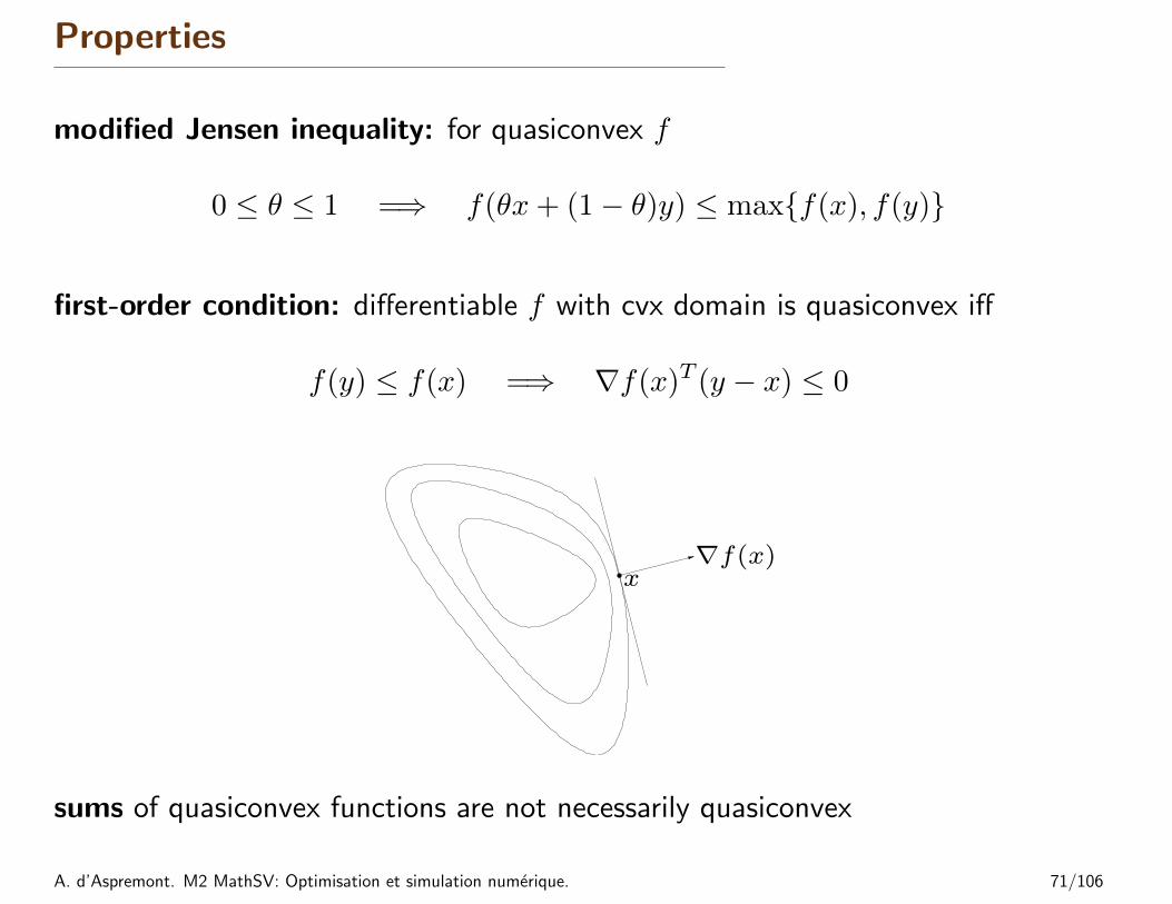
Properties
modified Jensen inequality: for quasiconvex f
0 ≤ θ ≤ 1 =⇒ f(θx+ (1− θ)y) ≤ max{f(x), f(y)}
first-order condition: differentiable f with cvx domain is quasiconvex iff
f(y) ≤ f(x) =⇒ ∇f(x)T (y − x) ≤ 0
x∇f(x)
sums of quasiconvex functions are not necessarily quasiconvex
A. d’Aspremont. M2 MathSV: Optimisation et simulation numerique. 71/106

Log-concave and log-convex functions
a positive function f is log-concave if log f is concave:
f(θx+ (1− θ)y) ≥ f(x)θf(y)1−θ for 0 ≤ θ ≤ 1
f is log-convex if log f is convex
� powers: xa on R++ is log-convex for a ≤ 0, log-concave for a ≥ 0
� many common probability densities are log-concave, e.g., normal:
f(x) =1√
(2π)n det Σe−
12(x−x)TΣ−1(x−x)
� cumulative Gaussian distribution function Φ is log-concave
Φ(x) =1√2π
∫ x
−∞e−u
2/2 du
A. d’Aspremont. M2 MathSV: Optimisation et simulation numerique. 72/106

Properties of log-concave functions
� twice differentiable f with convex domain is log-concave if and only if
f(x)∇2f(x) � ∇f(x)∇f(x)T
for all x ∈ dom f
� product of log-concave functions is log-concave
� sum of log-concave functions is not always log-concave
� integration: if f : Rn × Rm → R is log-concave, then
g(x) =
∫f(x, y) dy
is log-concave (not easy to show)
A. d’Aspremont. M2 MathSV: Optimisation et simulation numerique. 73/106

consequences of integration property
� convolution f ∗ g of log-concave functions f , g is log-concave
(f ∗ g)(x) =
∫f(x− y)g(y)dy
� if C ⊆ Rn convex and y is a random variable with log-concave pdf then
f(x) = Prob(x+ y ∈ C)
is log-concave
proof: write f(x) as integral of product of log-concave functions
f(x) =
∫g(x+ y)p(y) dy, g(u) =
{1 u ∈ C0 u 6∈ C,
p is pdf of y
A. d’Aspremont. M2 MathSV: Optimisation et simulation numerique. 74/106

Convex Optimization Problems
A. d’Aspremont. M2 MathSV: Optimisation et simulation numerique. 75/106

Outline
� optimization problem in standard form
� convex optimization problems
� quasiconvex optimization
� linear optimization
� quadratic optimization
� geometric programming
� generalized inequality constraints
� semidefinite programming
� vector optimization
A. d’Aspremont. M2 MathSV: Optimisation et simulation numerique. 76/106

Optimization problem in standard form
minimize f0(x)subject to fi(x) ≤ 0, i = 1, . . . ,m
hi(x) = 0, i = 1, . . . , p
� x ∈ Rn is the optimization variable
� f0 : Rn → R is the objective or cost function
� fi : Rn → R, i = 1, . . . ,m, are the inequality constraint functions
� hi : Rn → R are the equality constraint functions
optimal value:
p? = inf{f0(x) | fi(x) ≤ 0, i = 1, . . . ,m, hi(x) = 0, i = 1, . . . , p}
� p? =∞ if problem is infeasible (no x satisfies the constraints)
� p? = −∞ if problem is unbounded below
A. d’Aspremont. M2 MathSV: Optimisation et simulation numerique. 77/106

Optimal and locally optimal points
x is feasible if x ∈ dom f0 and it satisfies the constraints
a feasible x is optimal if f0(x) = p?; Xopt is the set of optimal points
x is locally optimal if there is an R > 0 such that x is optimal for
minimize (over z) f0(z)subject to fi(z) ≤ 0, i = 1, . . . ,m, hi(z) = 0, i = 1, . . . , p
‖z − x‖2 ≤ R
examples (with n = 1, m = p = 0)
� f0(x) = 1/x, dom f0 = R++: p? = 0, no optimal point
� f0(x) = − log x, dom f0 = R++: p? = −∞
� f0(x) = x log x, dom f0 = R++: p? = −1/e, x = 1/e is optimal
� f0(x) = x3 − 3x, p? = −∞, local optimum at x = 1
A. d’Aspremont. M2 MathSV: Optimisation et simulation numerique. 78/106

Implicit constraints
the standard form optimization problem has an implicit constraint
x ∈ D =
m⋂i=0
dom fi ∩p⋂i=1
domhi,
� we call D the domain of the problem
� the constraints fi(x) ≤ 0, hi(x) = 0 are the explicit constraints
� a problem is unconstrained if it has no explicit constraints (m = p = 0)
example:
minimize f0(x) = −∑ki=1 log(bi − aTi x)
is an unconstrained problem with implicit constraints aTi x < bi
A. d’Aspremont. M2 MathSV: Optimisation et simulation numerique. 79/106

Feasibility problem
find xsubject to fi(x) ≤ 0, i = 1, . . . ,m
hi(x) = 0, i = 1, . . . , p
can be considered a special case of the general problem with f0(x) = 0:
minimize 0subject to fi(x) ≤ 0, i = 1, . . . ,m
hi(x) = 0, i = 1, . . . , p
� p? = 0 if constraints are feasible; any feasible x is optimal
� p? =∞ if constraints are infeasible
A. d’Aspremont. M2 MathSV: Optimisation et simulation numerique. 80/106

Convex optimization problem
standard form convex optimization problem
minimize f0(x)subject to fi(x) ≤ 0, i = 1, . . . ,m
aTi x = bi, i = 1, . . . , p
� f0, f1, . . . , fm are convex; equality constraints are affine
� problem is quasiconvex if f0 is quasiconvex (and f1, . . . , fm convex)
often written asminimize f0(x)subject to fi(x) ≤ 0, i = 1, . . . ,m
Ax = b
important property: feasible set of a convex optimization problem is convex
A. d’Aspremont. M2 MathSV: Optimisation et simulation numerique. 81/106

example
minimize f0(x) = x21 + x2
2
subject to f1(x) = x1/(1 + x22) ≤ 0
h1(x) = (x1 + x2)2 = 0
� f0 is convex; feasible set {(x1, x2) | x1 = −x2 ≤ 0} is convex
� not a convex problem (according to our definition): f1 is not convex, h1 is notaffine
� equivalent (but not identical) to the convex problem
minimize x21 + x2
2
subject to x1 ≤ 0x1 + x2 = 0
A. d’Aspremont. M2 MathSV: Optimisation et simulation numerique. 82/106

Local and global optima
any locally optimal point of a convex problem is (globally) optimal
proof: suppose x is locally optimal and y is optimal with f0(y) < f0(x)
x locally optimal means there is an R > 0 such that
z feasible, ‖z − x‖2 ≤ R =⇒ f0(z) ≥ f0(x)
consider z = θy + (1− θ)x with θ = R/(2‖y − x‖2)
� ‖y − x‖2 > R, so 0 < θ < 1/2
� z is a convex combination of two feasible points, hence also feasible
� ‖z − x‖2 = R/2 and
f0(z) ≤ θf0(x) + (1− θ)f0(y) < f0(x)
which contradicts our assumption that x is locally optimal
A. d’Aspremont. M2 MathSV: Optimisation et simulation numerique. 83/106

Optimality criterion for differentiable f0
x is optimal if and only if it is feasible and
∇f0(x)T (y − x) ≥ 0 for all feasible y
−∇f0(x)
Xx
if nonzero, ∇f0(x) defines a supporting hyperplane to feasible set X at x
A. d’Aspremont. M2 MathSV: Optimisation et simulation numerique. 84/106

� unconstrained problem: x is optimal if and only if
x ∈ dom f0, ∇f0(x) = 0
� equality constrained problem
minimize f0(x) subject to Ax = b
x is optimal if and only if there exists a ν such that
x ∈ dom f0, Ax = b, ∇f0(x) +ATν = 0
� minimization over nonnegative orthant
minimize f0(x) subject to x � 0
x is optimal if and only if
x ∈ dom f0, x � 0,
{∇f0(x)i ≥ 0 xi = 0∇f0(x)i = 0 xi > 0
A. d’Aspremont. M2 MathSV: Optimisation et simulation numerique. 85/106

Equivalent convex problems
two problems are (informally) equivalent if the solution of one is readily obtainedfrom the solution of the other, and vice-versa
some common transformations that preserve convexity:
� eliminating equality constraints
minimize f0(x)subject to fi(x) ≤ 0, i = 1, . . . ,m
Ax = b
is equivalent to
minimize (over z) f0(Fz + x0)subject to fi(Fz + x0) ≤ 0, i = 1, . . . ,m
where F and x0 are such that
Ax = b ⇐⇒ x = Fz + x0 for some z
A. d’Aspremont. M2 MathSV: Optimisation et simulation numerique. 86/106

� introducing equality constraints
minimize f0(A0x+ b0)subject to fi(Aix+ bi) ≤ 0, i = 1, . . . ,m
is equivalent to
minimize (over x, yi) f0(y0)subject to fi(yi) ≤ 0, i = 1, . . . ,m
yi = Aix+ bi, i = 0, 1, . . . ,m
� introducing slack variables for linear inequalities
minimize f0(x)subject to aTi x ≤ bi, i = 1, . . . ,m
is equivalent to
minimize (over x, s) f0(x)subject to aTi x+ si = bi, i = 1, . . . ,m
si ≥ 0, i = 1, . . .m
A. d’Aspremont. M2 MathSV: Optimisation et simulation numerique. 87/106
� epigraph form: standard form convex problem is equivalent to
minimize (over x, t) tsubject to f0(x)− t ≤ 0
fi(x) ≤ 0, i = 1, . . . ,mAx = b
� minimizing over some variables
minimize f0(x1, x2)subject to fi(x1) ≤ 0, i = 1, . . . ,m
is equivalent to
minimize f0(x1)subject to fi(x1) ≤ 0, i = 1, . . . ,m
where f0(x1) = infx2 f0(x1, x2)
A. d’Aspremont. M2 MathSV: Optimisation et simulation numerique. 88/106
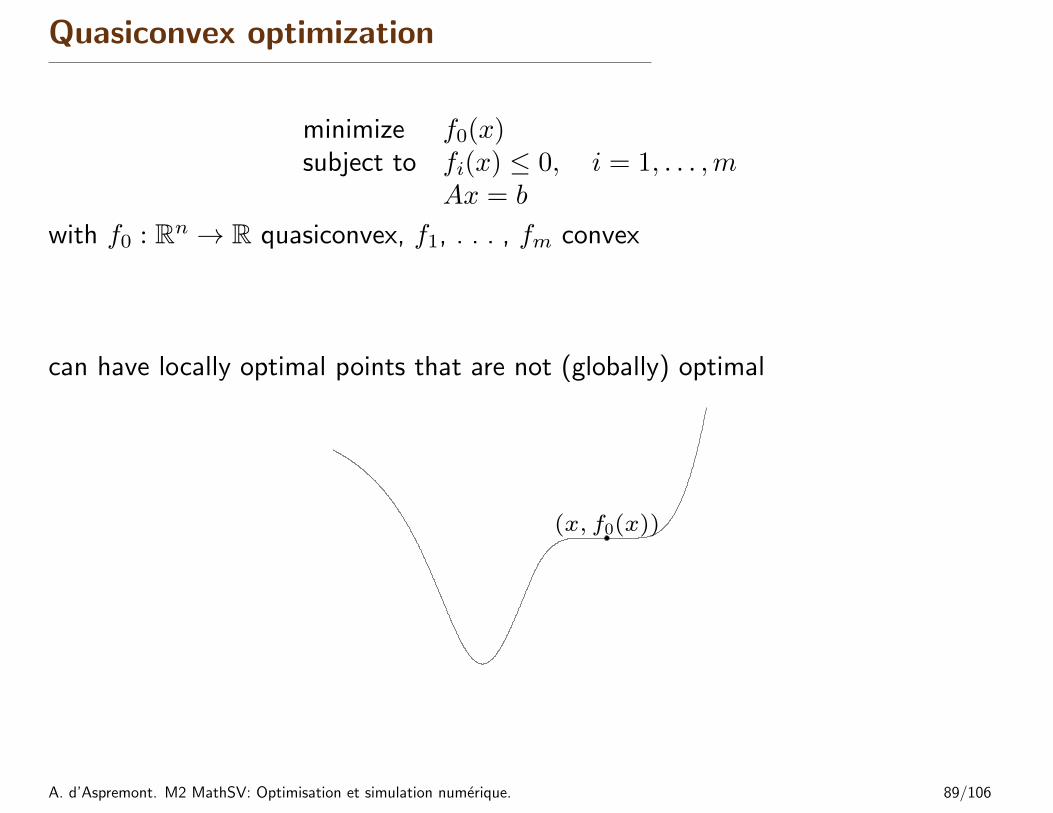
Quasiconvex optimization
minimize f0(x)subject to fi(x) ≤ 0, i = 1, . . . ,m
Ax = b
with f0 : Rn → R quasiconvex, f1, . . . , fm convex
can have locally optimal points that are not (globally) optimal
(x, f0(x))
A. d’Aspremont. M2 MathSV: Optimisation et simulation numerique. 89/106

quasiconvex optimization via convex feasibility problems
f0(x) ≤ t, fi(x) ≤ 0, i = 1, . . . ,m, Ax = b (1)
� for fixed t, a convex feasibility problem in x
� if feasible, we can conclude that t ≥ p?; if infeasible, t ≤ p?
Bisection method for quasiconvex optimization
given l ≤ p?, u ≥ p?, tolerance ε > 0.
repeat1. t := (l + u)/2.2. Solve the convex feasibility problem (1).3. if (1) is feasible, u := t; else l := t.
until u− l ≤ ε.
requires exactly dlog2((u− l)/ε)e iterations (where u, l are initial values)
A. d’Aspremont. M2 MathSV: Optimisation et simulation numerique. 90/106

Linear program (LP)
minimize cTx+ dsubject to Gx � h
Ax = b
� convex problem with affine objective and constraint functions
� feasible set is a polyhedron
Px⋆
−c
A. d’Aspremont. M2 MathSV: Optimisation et simulation numerique. 91/106

Examples
diet problem: choose quantities x1, . . . , xn of n foods
� one unit of food j costs cj, contains amount aij of nutrient i
� healthy diet requires nutrient i in quantity at least bi
to find cheapest healthy diet,
minimize cTxsubject to Ax � b, x � 0
piecewise-linear minimization
minimize maxi=1,...,m(aTi x+ bi)
equivalent to an LP
minimize tsubject to aTi x+ bi ≤ t, i = 1, . . . ,m
A. d’Aspremont. M2 MathSV: Optimisation et simulation numerique. 92/106

Chebyshev center of a polyhedron
Chebyshev center of
P = {x | aTi x ≤ bi, i = 1, . . . ,m}
is center of largest inscribed ball
B = {xc + u | ‖u‖2 ≤ r}
xchebxcheb
� aTi x ≤ bi for all x ∈ B if and only if
sup{aTi (xc + u) | ‖u‖2 ≤ r} = aTi xc + r‖ai‖2 ≤ bi
� hence, xc, r can be determined by solving the LP
maximize rsubject to aTi xc + r‖ai‖2 ≤ bi, i = 1, . . . ,m
A. d’Aspremont. M2 MathSV: Optimisation et simulation numerique. 93/106

(Generalized) linear-fractional program
minimize f0(x)subject to Gx � h
Ax = b
linear-fractional program
f0(x) =cTx+ d
eTx+ f, dom f0(x) = {x | eTx+ f > 0}
� a quasiconvex optimization problem; can be solved by bisection
� also equivalent to the LP (variables y, z)
minimize cTy + dzsubject to Gy � hz
Ay = bzeTy + fz = 1z ≥ 0
A. d’Aspremont. M2 MathSV: Optimisation et simulation numerique. 94/106

Quadratic program (QP)
minimize (1/2)xTPx+ qTx+ rsubject to Gx � h
Ax = b
� P ∈ Sn+, so objective is convex quadratic
� minimize a convex quadratic function over a polyhedron
P
x⋆
−∇f0(x⋆)
A. d’Aspremont. M2 MathSV: Optimisation et simulation numerique. 95/106

Examples
least-squaresminimize ‖Ax− b‖22
� analytical solution x? = A†b (A† is pseudo-inverse)
� can add linear constraints, e.g., l � x � u
linear program with random cost
minimize cTx+ γxTΣx = E cTx+ γ var(cTx)subject to Gx � h, Ax = b
� c is random vector with mean c and covariance Σ
� hence, cTx is random variable with mean cTx and variance xTΣx
� γ > 0 is risk aversion parameter; controls the trade-off between expected costand variance (risk)
A. d’Aspremont. M2 MathSV: Optimisation et simulation numerique. 96/106

Quadratically constrained quadratic program (QCQP)
minimize (1/2)xTP0x+ qT0 x+ r0
subject to (1/2)xTPix+ qTi x+ ri ≤ 0, i = 1, . . . ,mAx = b
� Pi ∈ Sn+; objective and constraints are convex quadratic
� if P1, . . . , Pm ∈ Sn++, feasible region is intersection of m ellipsoids and anaffine set
A. d’Aspremont. M2 MathSV: Optimisation et simulation numerique. 97/106

Second-order cone programming
minimize fTxsubject to ‖Aix+ bi‖2 ≤ cTi x+ di, i = 1, . . . ,m
Fx = g
(Ai ∈ Rni×n, F ∈ Rp×n)
� inequalities are called second-order cone (SOC) constraints:
(Aix+ bi, cTi x+ di) ∈ second-order cone in Rni+1
� for ni = 0, reduces to an LP; if ci = 0, reduces to a QCQP
� more general than QCQP and LP
A. d’Aspremont. M2 MathSV: Optimisation et simulation numerique. 98/106
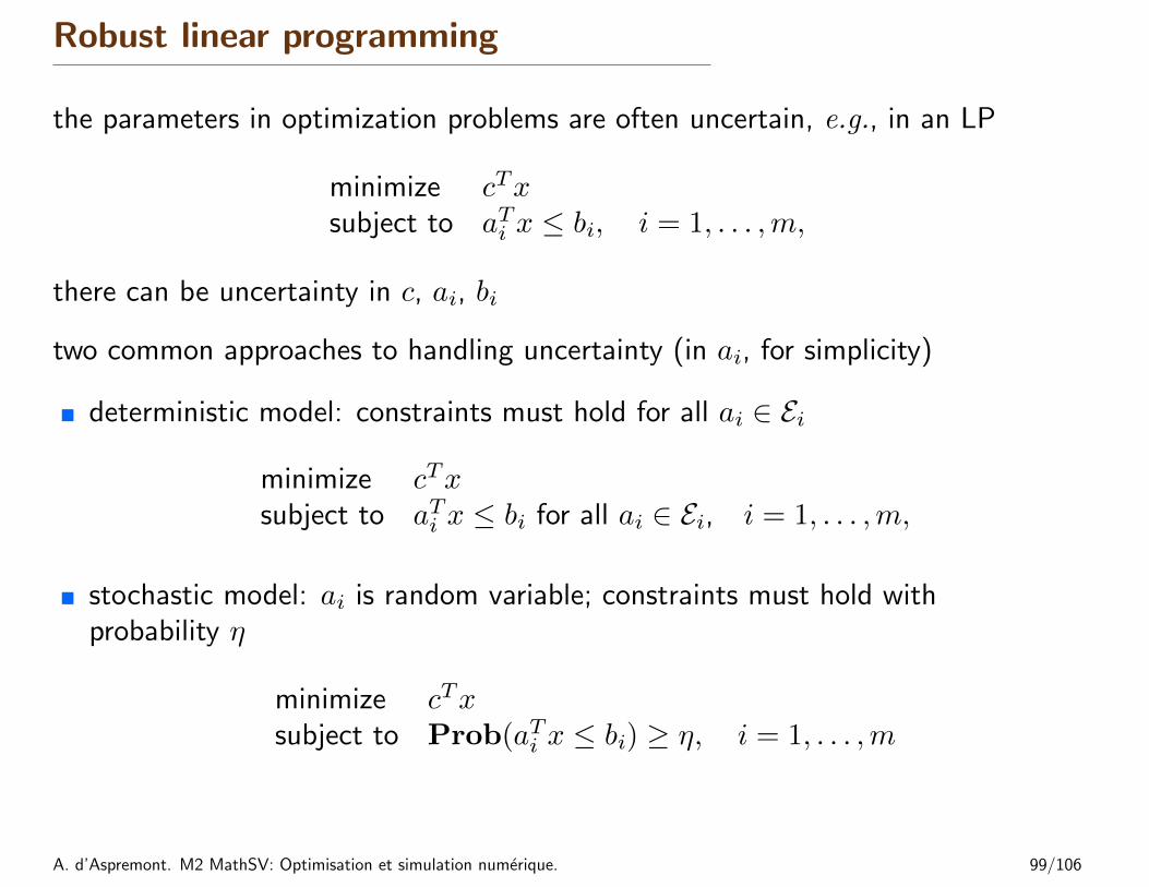
Robust linear programming
the parameters in optimization problems are often uncertain, e.g., in an LP
minimize cTxsubject to aTi x ≤ bi, i = 1, . . . ,m,
there can be uncertainty in c, ai, bi
two common approaches to handling uncertainty (in ai, for simplicity)
� deterministic model: constraints must hold for all ai ∈ Ei
minimize cTxsubject to aTi x ≤ bi for all ai ∈ Ei, i = 1, . . . ,m,
� stochastic model: ai is random variable; constraints must hold withprobability η
minimize cTxsubject to Prob(aTi x ≤ bi) ≥ η, i = 1, . . . ,m
A. d’Aspremont. M2 MathSV: Optimisation et simulation numerique. 99/106

deterministic approach via SOCP
� choose an ellipsoid as Ei:
Ei = {ai + Piu | ‖u‖2 ≤ 1} (ai ∈ Rn, Pi ∈ Rn×n)
center is ai, semi-axes determined by singular values/vectors of Pi
� robust LP
minimize cTxsubject to aTi x ≤ bi ∀ai ∈ Ei, i = 1, . . . ,m
is equivalent to the SOCP
minimize cTxsubject to aTi x+ ‖PTi x‖2 ≤ bi, i = 1, . . . ,m
(follows from sup‖u‖2≤1(ai + Piu)Tx = aTi x+ ‖PTi x‖2)
A. d’Aspremont. M2 MathSV: Optimisation et simulation numerique. 100/106

stochastic approach via SOCP
� assume ai is Gaussian with mean ai, covariance Σi (ai ∼ N (ai,Σi))
� aTi x is Gaussian r.v. with mean aTi x, variance xTΣix; hence
Prob(aTi x ≤ bi) = Φ
(bi − aTi x‖Σ1/2
i x‖2
)
where Φ(x) = (1/√
2π)∫ x−∞ e
−t2/2 dt is CDF of N (0, 1)
� robust LP
minimize cTxsubject to Prob(aTi x ≤ bi) ≥ η, i = 1, . . . ,m,
with η ≥ 1/2, is equivalent to the SOCP
minimize cTx
subject to aTi x+ Φ−1(η)‖Σ1/2i x‖2 ≤ bi, i = 1, . . . ,m
A. d’Aspremont. M2 MathSV: Optimisation et simulation numerique. 101/106
Generalized inequality constraints
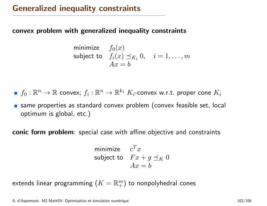
convex problem with generalized inequality constraints
minimize f0(x)subject to fi(x) �Ki 0, i = 1, . . . ,m
Ax = b
� f0 : Rn → R convex; fi : Rn → Rki Ki-convex w.r.t. proper cone Ki
� same properties as standard convex problem (convex feasible set, localoptimum is global, etc.)
conic form problem: special case with affine objective and constraints
minimize cTxsubject to Fx+ g �K 0
Ax = b
extends linear programming (K = Rm+ ) to nonpolyhedral cones
A. d’Aspremont. M2 MathSV: Optimisation et simulation numerique. 102/106

Semidefinite program (SDP)
minimize cTxsubject to x1F1 + x2F2 + · · ·+ xnFn +G � 0
Ax = b
with Fi, G ∈ Sk
� inequality constraint is called linear matrix inequality (LMI)
� includes problems with multiple LMI constraints: for example,
x1F1 + · · ·+ xnFn + G � 0, x1F1 + · · ·+ xnFn + G � 0
is equivalent to single LMI
x1
[F1 0
0 F1
]+ x2
[F2 0
0 F2
]+ · · ·+ xn
[Fn 0
0 Fn
]+
[G 0
0 G
]� 0
A. d’Aspremont. M2 MathSV: Optimisation et simulation numerique. 103/106
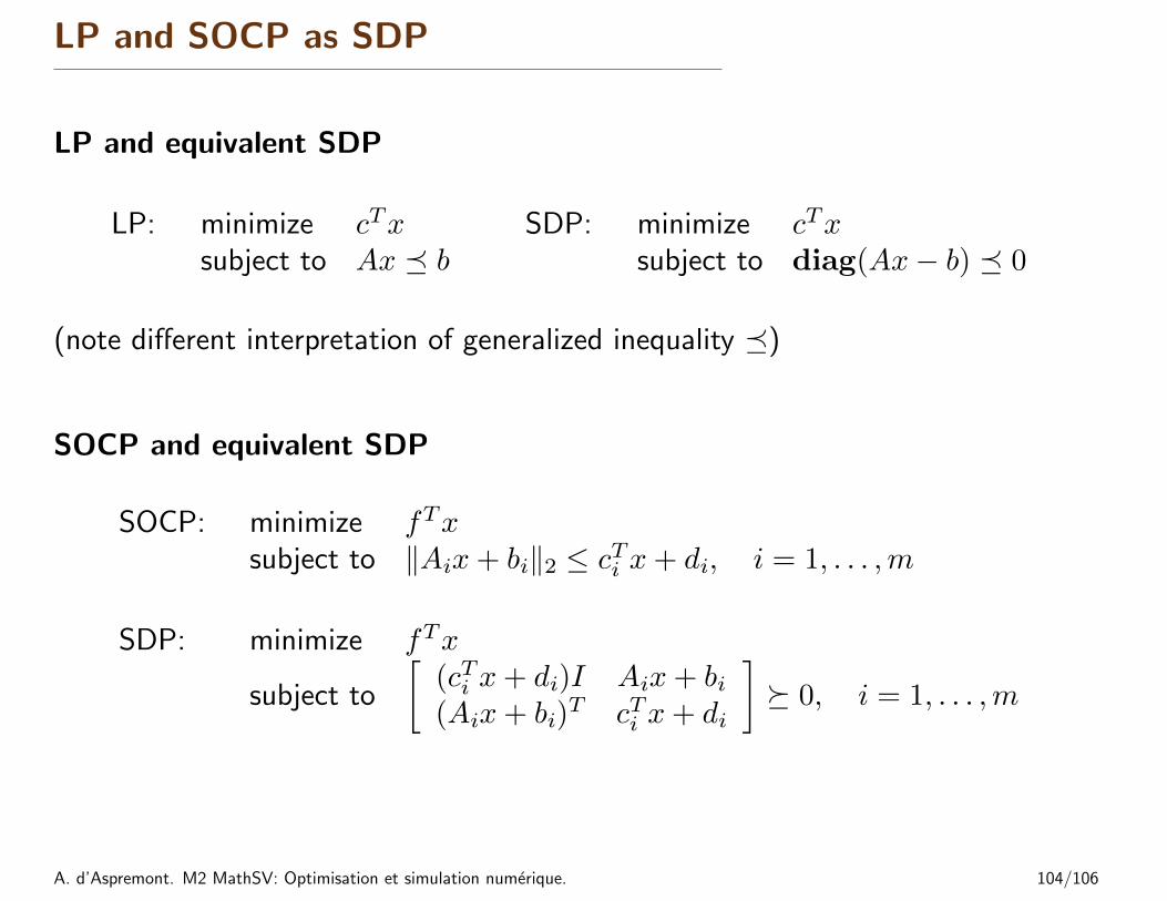
LP and SOCP as SDP
LP and equivalent SDP
LP: minimize cTxsubject to Ax � b
SDP: minimize cTxsubject to diag(Ax− b) � 0
(note different interpretation of generalized inequality �)
SOCP and equivalent SDP
SOCP: minimize fTxsubject to ‖Aix+ bi‖2 ≤ cTi x+ di, i = 1, . . . ,m
SDP: minimize fTx
subject to
[(cTi x+ di)I Aix+ bi(Aix+ bi)
T cTi x+ di
]� 0, i = 1, . . . ,m
A. d’Aspremont. M2 MathSV: Optimisation et simulation numerique. 104/106

Eigenvalue minimization
minimize λmax(A(x))
where A(x) = A0 + x1A1 + · · ·+ xnAn (with given Ai ∈ Sk)
equivalent SDPminimize tsubject to A(x) � tI
� variables x ∈ Rn, t ∈ R
� follows fromλmax(A) ≤ t ⇐⇒ A � tI
A. d’Aspremont. M2 MathSV: Optimisation et simulation numerique. 105/106

Matrix norm minimization
minimize ‖A(x)‖2 =(λmax(A(x)TA(x))
)1/2where A(x) = A0 + x1A1 + · · ·+ xnAn (with given Ai ∈ Sp×q)
equivalent SDPminimize t
subject to
[tI A(x)
A(x)T tI
]� 0
� variables x ∈ Rn, t ∈ R
� constraint follows from
‖A‖2 ≤ t ⇐⇒ ATA � t2I, t ≥ 0
⇐⇒[tI AAT tI
]� 0
A. d’Aspremont. M2 MathSV: Optimisation et simulation numerique. 106/106

*
References
A. Ben-Tal and A. Nemirovski. Lectures on modern convex optimization : analysis, algorithms, and engineering applications. MPS-SIAMseries on optimization. Society for Industrial and Applied Mathematics : Mathematical Programming Society, Philadelphia, PA, 2001.
N. K. Karmarkar. A new polynomial-time algorithm for linear programming. Combinatorica, 4:373–395, 1984.
L. G. Khachiyan. A polynomial algorithm in linear programming (in Russian). Doklady Akademiia Nauk SSSR, 224:1093–1096, 1979.
A. Nemirovskii and D. Yudin. Problem complexity and method efficiency in optimization. Nauka (published in English by John Wiley,Chichester, 1983), 1979.
Y. Nesterov. Introductory Lectures on Convex Optimization. Springer, 2003.
Y. Nesterov and A. Nemirovskii. Interior-point polynomial algorithms in convex programming. Society for Industrial and AppliedMathematics, Philadelphia, 1994.
A. d’Aspremont. M2 MathSV: Optimisation et simulation numerique. 107/106