DOI 10.1007/s00158-004-0502-0

RESEARCH PAPER

Struct Multidisc Optim (2005) 30: 101–112

S. Turteltaub

Optimal non-homogeneous composites for dynamic loading

Received: 4 August 2004 / Revised manuscript received: 6 October 2004 / Published online: 17 February 2005 Springer-Verlag 2005

Abstract An algorithm is proposed to optimize the per-formance of a two-phase composite under dynamic loading.The goal is to determine a series of different layouts of thetwo base materials in a three-dimensional region such thatthe time-averaged stress energy is minimized. Four caseswith different boundary conditions and ratios of mass dens-ity are considered and solved numerically. The resultingoptimal designs are compared to the static case to illustratethe effect of the dynamic loading. Furthermore, a qualita-tive comparison is done to indicate the difference betweenthe optimization of eigenfrequencies and the present formu-lation.

Keywords Optimal design · Functionally graded material ·Inverse problem · Parameter identification · Stress waves

1 Introduction

The performance of composite materials can be improvedby considering a non-homogeneous layout instead of a ho-mogeneous one. Such layouts may be obtained through anoptimization procedure that tailors the material to a specificapplication, resulting in the so-called functionally gradedmaterials (FGMs, see e.g., Suresh and Mortensen (1998)).A non-homogeneous composite material can be though ofas a “structure”, hence, for convenience, that term will beused when referring to a FGM that occupies a region Ω. Anoptimal design corresponds to specifying a particular layoutthat outperforms all others by minimizing or maximizing anobjective functional (measure of performance).

Optimal design of material and structures is often car-ried out in a static framework. Typical examples includethe minimum structural compliance problem (i.e., maximumstructural stiffness) and maximization or minimization ofmaterial properties (e.g., bulk or shear modulus). However,in many practical situations it is important to take into ac-count the transient response, such as in impact problems. In

S. TurteltaubFaculty of Aerospace Engineering, Delft University of Technology,Kluyverweg 1, NL-2629 HS Delft, The NetherlandsE-mail: s.r.turteltaub@lr.tudelft.nl

the present communication, an algorithm is proposed to op-timize the performance of a two-phase composite under dy-namic loading. In particular, as explained below in Sect. 3,the goal is to determine a series of different layouts of thetwo base materials such that the time-averaged stress energyis sequentially minimized.

The motivation for this choice of the objective functionalstems from several considerations. Under dynamic loading,different stress waves propagate throughout the solid. Dueto the inhomogeneity of the material, the decoupling ofstress waves inside the solid into pressure and shear wavesis in general not possible. Furthermore, due to the finite sizeof a three-dimensional specimen, further reflections gener-ate a relatively complex transient stress distribution whichmay differ considerably from its quasi-static counterpart. Inthe optimal design problem, the purpose is to utilize thebase materials efficiently for the corresponding stress waves,though of course this is a coupled inverse problem since thewave pattern depends in turn on the layout of the two mate-rials.

Optimal design under impact loads has been analyzed inthe one-dimensional case1 (Bruck 2000; Velo et al. 2002),where the objective was to reduce the amplitude of the stresswaves. It was found that a time delay can be achieved, butthat any reinforcement leads to higher stresses (which issimilar to what happens in the static case). This is not nec-essarily a problem since the stresses need to be comparedto a failure criterion, which itself depends on the amountand type of reinforcement, but it highlights the fact that re-duction of stresses alone might not be a practical objectivefunctional.

A class of problems related to dynamic loading is themaximization of the smallest eigenvalue of a structure infree vibration (Dıaz and Kikuchi 1992; Krog and Olhoff1999; Allaire et al. 2001). That problem, however, is onlyindirectly related to the transient response of a particularloading case. Moreover, maximization of the smallest eigen-value in free vibration may occur at the expense of othereigenvalues (whose magnitude might be reduced). In that

1 For zero displacement boundary conditions on the end opposite tothe applied loads.

102 S. Turteltaub

case the solution to the max-min eigenvalue problem mightnot be optimal for a given design load that, e.g., activatespreferentially one or several higher vibration modes (an ex-ample that illustrates this situation is shown in Sect. 7).

In view of the previous considerations, the goal of thepresent communication is to identify a suitable objectivefunctional and to develop a solution method for the designproblem that takes into account the transient response ofa particular loading case. To this end, the paper is dividedas follows: Section 2 contains preliminary definitions thatwill be used throughout the paper, including the materialmodel. The definition of the objective functional and the for-mulation of the problem are presented in Sect. 3. In Sect. 4,the gradient of the objective functional is computed and thecorresponding numerical algorithm to solve the optimiza-tion problem is summarized. Examples of optimal designare presented in Sect. 5 where the effect of different typesof boundary conditions and ratios of mass density of thebase materials are analyzed. In Sect. 6, the performance ofthe optimal designs obtained in Sect. 5 are computed forlonger analysis times to assess their behavior outside of theoptimization time interval. Further analysis of the optimalsolutions is shown in Sect. 7. In particular, the optimal de-signs are compared to the corresponding quasi-static onesand, additionally, the effect of the optimization procedureon the lowest eigenvalue is quantified. Finally, some closingremarks are included in Sect. 8.

It is worth pointing out that, although the composite be-ing designed is assumed to be an elastic material, the cor-responding optimal design problem using variable materialproperties is a non-linear path-dependent problem with sev-eral inequality constraints and thus it has common featureswith inelastic behavior. The path dependency of the designproblem has been illustrated in the case of quasi-static, non-proportional loading in Turteltaub (2002b)

2 Preliminaries

Starting from a set of arbitrary two-phase microstructures,Allaire et al. (2001) proved the optimality of rank-N lami-nates in a problem where they optimize the (macroscopic)eigenfrequency of a composite in a domain Ω. A similarresult was shown earlier for the optimization of the (macro-scopic) compliance, see Lipton (1994). A common charac-teristic of the examples mentioned above is that the com-bined design/objective functional problem corresponds toa max-min (or min-max) formulation: the objective func-tional is computed minimizing or maximizing a functionalwith respect to field variables (the inner problem) while theouter design problem corresponds to maximizing or mini-mizing the objective functional. Since those problems admita saddle point, then the outer and inner problems can be(partially) exchanged. The application of the saddle pointtheorem, where rank-N laminates are shown to be opti-mal microstructures, simplifies the design problem to thesearch of optimal (local) volume fractions of the laminates(see Bendsøe and Sigmund (2002) for a comprehensive re-view).

In contrast, the present formulation, as shown below,is only a minimization problem (i.e., minimization of theobjective functional). The objective functional, definedin Sect. 3, cannot be obtained from a maximum or minimumprinciple. The main reason for this limitation is that in dy-namics there is no counterpart to the minimum or maximumprinciples that characterize the static or the eigenfrequencyproblems.

In view of the previous considerations and in order tokeep the problem computationally tractable, we choose torestrict attention to a smaller class of two-phase composites.In particular, the FGM is assumed to be (i) macroscopi-cally isotropic and (ii) its effective properties are assumed todepend only on the local volume fraction. Although these as-sumptions restrict the class of admissible designs, it still re-mains technologically relevant in the sense that many FGMsapproximately satisfy these assumptions. In particular, it isassumed that the effective properties are given as the aver-age between the Hashin–Shtrikman upper and lower bounds(Hashin and Shtrikman 1963), which provide a good ap-proximation for two-phase composites of moderate contrast2

and are automatically consistent with the bounds.Consider a simply connected regular domain Ω with

boundary ∂Ω. Inside the domain Ω there is an inhomoge-neous two-phase FGM. The effective material properties aremodelled as functions of the volume fraction ω = ω(x) ofone the phases in a representative volume element centeredat a point x. For definiteness, suppose that ω is the vol-ume fraction of material 1. At each point x ∈ Ω, the volumefraction ω(x) is henceforth referred to as the design vari-able. It is assumed that the composite is made out of particleinclusions where the size of a characteristic inclusion is suf-ficiently small compared to the dimensions of a specimenso that there is a clear separation of scales. Further, the roleof matrix and inclusions is reversed as ω varies from 0 to1. Variations of ω in space are assumed to be small com-pared to the size of the inclusions and second-order effectsdue to spatially varying volume fractions are neglected whencomputing properties at each point x.

Let C = C(ω(x)) be the effective elasticity tensor andρ = ρ(ω(x)) the mass density. The effective stress σ isgiven by σ = Cε, where ε = 1

2 (∇u+∇uT ) is the effectivestrain tensor and u the displacement. Introduce the follow-ing fourth-order tensors: H := 1

3 I ⊗ I, J := I−H, where Iand I are the second- and fourth-order (symmetric) identitytensors, respectively. For the isotropic case, one has

C = ebH+ esJ , D = e−1b H+ e−1

s J , eb = 3κ , es = 2µ ,

where D = C−1 is the compliance tensor, eb and es arethe distinct eigenvalues of C, κ is the bulk modulus andµ the shear modulus. For design purposes, suppose thatone has available two homogeneous, isotropic, linear ma-terials (i = 1, 2) with respective properties κi , µi and massdensities ρi . The effective properties are given by func-tions κ = κ(κi, µi, ω), µ = µ(κi, µi, ω) and ρ = ρ(ρi, ω),

2 See Turteltaub (2002b) for the case of Ni/Al2O3.

Optimal non-homogeneous composites for dynamic loading 103

which depend on ω = ω(x) (the volume fraction of material1 in a representative volume element). Although the presentmodel characterizes the microstructure using a single pa-rameter ω, one can in principle consider a larger class ofcomposites if higher-order data are included.

Fields and properties can be viewed as functions of pos-ition and/or time as well as functions of the local volumefraction. To avoid additional notation the functions and theirvalues are denoted by the same letter whenever the mean-ing is clear by the context. The type of FGM consideredin this analysis is, for example, a ceramic-metal compositewith continuously varying volume fraction. A restriction onthe admissible functions ω is that they have to be continu-ous functions of x. Moreover, fluctuations of displacementsinside a representative element volume are averaged andthe effect of inhomogeneities are only measured at a lengthscale large enough to reflect changes in volume fraction.

For a given field ω, the displacement field is inter-preted as an implicit function of the material properties (i.e.,u = u[ω]) since it corresponds to the solution to the follow-ing dynamic process:

div σ = ρu in Ω × (0, T ] ,

σ(x, t)n = t(x, t) on ∂Ωt × (0, T ] ,

u(x, t) = u(x, t) on ∂Ωu × (0, T ] ,

u(x, 0) = u0(x) in Ω ,

u(x, 0) = v0(x) in Ω ,

(1)

where σ = C(ω)ε is the effective stress, n is the normal out-ward unit vector to the boundary ∂Ω and t, u, u0 and v0 aregiven functions. For simplicity, it is assumed that u = 0 andthat u0 is consistent with this assumption3. To avoid usingdifferent symbols, the same letters are used to designate thefields when viewed as functions of position and time (fora fixed ω) as well as when they are interpreted as implicitfunctions of ω (i.e., for each ω there are different fields thatsatisfy (1)). The spatial gradient and time derivative of thedisplacement are always interpreted for fixed ω. The nota-tion fω corresponds to the gradient of a field f interpretedas a function of ω (i.e., it measures changes in the field whendifferent distributions of material properties are considered).

3 Formulation of the problem

3.1 Definition of the objective functional

As mentioned in the introduction, there is a need to definean appropriate objective functional for the dynamics prob-lem. To this end, we use as a guideline an objective func-tional used in the static problem and look for an extensionto the dynamic case. Let ∂Ω = ∂Ωu ∪ ∂Ωt be the bound-ary of the domain occupied by the material. For simpli-city, we will assume henceforth that only zero displacementboundary conditions are prescribed on ∂Ωu while non-zero

3 The case of non-zero displacements for the quasi-static problem isanalyzed in Turteltaub (2002b).

traction is prescribed on ∂Ωt . Under that assumption, theminimum compliance problem for a static problem is equiva-lent to minimization of the strain energy4. The structure ornon-homogeneous material that minimizes the complianceis identified as having maximum stiffness. That formulation,however, cannot be extended to the dynamic setting (or thecase of non-proportional quasi-static loading) without an ad-ditional complication since, in a closed cycle for an elasticmaterial, the work done is zero and thus any material wouldbe trivially optimal. To circumvent this problem, the objec-tive functional used in the present formulation is definedbased on the loading path and the stress history.

Suppose that we have a system that starts from a strain-free state. The stress energy at time t for a process in a timeinterval [0, t] is

U [σ, t] := 1

2

∫

Ω

σ(x, t) ·D(x)σ(x, t) dv . (2)

The measure used in this paper to qualify an optimal de-sign is based on integrating the stress energy throughouta process in a given time interval of interest [0, T ], i.e., theobjective functional J is defined as follows:

J[ω] :=T∫

0

U[σ, t] dt . (3)

The domain Ω, the time interval [0, T ], the properties of thebase materials and the loads are considered to be given de-sign parameters. As such, they are not determined by thephysics of the problem directly but rather by design con-siderations of the specific problem being solved. Althoughthe choice of the time T is in principle arbitrary, it is notedthat a large T would typically correspond to a design thatis mostly concerned with the steady-state response whereasa small T corresponds to a design where the transient re-sponse is of primary interest. Even though no a priori restric-tions are imposed on the value of T , the present formulationis geared towards the latter due to computational cost. Asa guideline, one can choose the time T such that it capturesa few stress waves reflections based on a characteristic wavespeed of the base materials and a characteristic length of Ω.

The objective functional J is seen as a function of ω(x)

only since the stress field can be obtained as the solution toproblem (1). From this point of view, using the stress en-ergy is equivalent to using the strain energy in the objectivefunctional. Moreover, the objective functional, in a quasi-static process under proportional loading, coincides with theclassical formulation of the minimum compliance problemfor the static case with prescribed tractions on ∂Ωt and zerodisplacement on ∂Ωu .

The values of the volume fraction ω are constrained to liein the interval [ωm, ωM], with 0 ≤ ωm ≤ ωM ≤ 1. In the ex-amples shown in subsequent sections, the “box constraints”

4 For non-zero displacements and zero traction, the minimum compli-ance problem in the static case is equivalent to maximization of thestrain energy.

104 S. Turteltaub

are chosen as ωm = 0 and ωM = 1. To avoid trivial solutions,a global constraint on ω is enforced (the so-called resourceconstraint). The integral of ω over the design domain is as-sumed to lie below some value R, which is chosen from theoutset, i.e.,∫

Ω

ω dv ≤ R . (4)

In this case, the value R (such that 0 < R ≤ vol(Ω)) serves tobound the total amount of material 1 (reinforcement) used.Observe that the bound is specified in terms of volume andnot in terms of mass. Further, the objective functional doesnot include a term related to the kinetic energy, so that the re-inforcement is achieved through stiffness only, regardless ofwhether the mass density of the reinforcement is higher thanthat of material 2 or not. Results for different mass densityratios are presented in Sect. 5.

3.2 Formulation of the problem

Define the design space A as

A :=

ω | ω continuous in Ω ,

ωm ≤ ω ≤ ωM ,

∫

Ω

ω dv ≤ R

.

The design space should be a closed set. Since a sequence ofcontinuous functions can tend to a discontinuous function, itis not closed. This can potentially lead to a mesh-dependentnumerical solution. There are several ways to address thisproblem (see, e.g., Sigmund and Petersson (1998) for a re-view). In particular, one can restrict the admissible functionswith a penalty constraint5.

With the interpretation that the stress field in (3) is ob-tained from (1), the optimization problem can be expressedas follows:

Find ω0 ∈A such thatJ[ω0] ≤ J[ω] ∀ω ∈A .

(5)

4 Gradient of the objective functional and numericalalgorithm

4.1 Gradient

There are several methods that one could use to solve the op-timal layout problem. The method used here is based on thegradient of the objective functional with respect to layoutsof material properties. Its computation is outlined in this

5 Details can be found in Turteltaub (2002a). For the specific problemstreated in the present communication, this issue did not arise in thesense that a penalty constraint used in the numerical simulations wasnot active.

section. Since there is one objective functional and an infi-nite number of design variables ω(x) (in the continuum casethere is one variable for each point), then an adjoint tech-nique is particularly convenient instead of a direct method(see e.g., Kleiber et al. (1997), Dems and Mroz (1998)).

In order to compute the gradient of the objectivefunctional with respect to the design function ω(x), firstaugment J with the local constraints ωm − ω ≤ 0 andω−ωM ≤ 0 and the global constraint

∫

Ωω dv − R ≤ 0.

Introduce the corresponding Lagrange multiplier fieldsλm(x) ≥ 0 and λM(x) ≥ 0 for the local constraints and theLagrange multiplier Λ ≥ 0 for the global constraint as fol-lows:

L[ω, λm, λM,Λ] := J[ω]+∫

Ω

λm(ωm −ω) dv

+∫

Ω

λM(ω−ωM) dv+Λ

∫

Ω

ω dv− R

. (6)

A direct calculation using (2), (3) and (6) shows that the firstvariation of L with respect to ω is formally given by

δL[ω, λm, λM,Λ; δω] =T∫

0

∫

Ω

Dσ · δσ dv dt

+ 1

2

T∫

0

∫

Ω

Dωσ ·σ δω dv dt

+∫

Ω

(−λm +λM +Λ)δω dv , (7)

where δσ(x, t) measures the difference in stress for two dif-ferent distributions of volume fraction ω1 and ω2 such thatω2(x) = ω1(x)+ δω(x). The subscript ω indicates differen-tiation with respect to volume fractions, i.e., (·)ω = ∂(·)/∂ω.

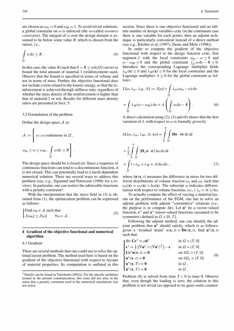
To actually compute the effect of varying a material lay-out on the performance of the FGM, one has to solve anadjoint problem with adjoint “constitutive” relations (i.e.,the purpose is to compute δσ). Let u∗ be a vector-valuedfunction, ε∗ and σ∗ tensor-valued functions (assumed to besymmetric) defined in Ω ×[0, T ].

Following the adjoint method, one can identify the ad-joint problem that u∗ should satisfy, which is as follows:given a “residual strain” ε(x, t) = Dσ(x, t), find u∗(x, t)such that

div Cε∗ = ρu∗ in Ω × (T, 0]ε∗ = 1

2

(∇u∗ + (∇u∗)T)− ε in Ω × (T, 0]

Cε∗n(x, t) = 0 on ∂Ωt × (T, 0]u∗(x, t) = 0 on ∂Ωu × (T, 0]u∗(x, T ) = 0 in Ω ,

u∗(x, T ) = 0 in Ω .

(8)

Problem (8) is solved from time T > 0 to time 0. Observethat, even though the loading is zero, the solution to thisproblem is not trivial (as opposed to its quasi-static counter-

Optimal non-homogeneous composites for dynamic loading 105

part). For computational purposes, it is useful to introducethe adjoint time variable τ := T − t. Using τ instead of t theproblem can be solved from 0 to T . Using the solution to theadjoint problem, one can show that

T∫

0

∫

Ω

Dσ · δσ dv dt =

−T∫

0

∫

Ω

(ε∗ ·Cωε+ρωu∗ · u

)δω dv dt .

In view of (7) and the previous relation, the first variation ofL can be written as

δL[ω, λm, λM,Λ; δω] =∫

Ω

L ′δω dv , (9)

where the gradient of the augmented objective functional Lis

L ′(x) = g(x)+ f(x)−λm(x)+λM(x)+Λ , (10)

and the functions f (explicit gradient of J) and g (implicitgradient of J) are given by

f(x) := 1

2

T∫

0

Dωσ ·σ dt (11)

and

g(x) := −T∫

0

ε∗ ·Cωε+ρωu∗ · u

dt . (12)

The necessary conditions for the optimal solution ω0 fol-low from the first-order Karush–Kuhn–Tucker conditions.For brevity, these are not listed here.

4.2 Numerical implementation

The algorithm used for the solution of problem (5) is basedon the gradient L ′. Since the design problem is non-linear,an iterative scheme is used to find a numerical approxima-tion of the solution. Details on implementation of a gradient-based method can be found in Turteltaub (2002a,b), thoughsome remarks pertinent to the present problem are includedhere.

The procedure starts from an arbitrary configurationω(0) = ω(0)(x). At some iteration n, with an approximationω(n) for the optimal distribution of volume fractions, all ef-fective material properties can be computed for all points xat the level of integration points. The strain ε(x, t) can beobtained by solving problem (1). Subsequently, ε(x, t) isintroduced as a time-dependent residual strain in the ad-joint problem (8), which can be solved to obtain u∗ andε∗. The direct and adjoint fields are then combined in (11)

and (12) to compute f(x) and g(x). It is worth noticing that,for a more efficient numerical implementation, the functionsf and g admit other equivalent expressions. Indeed, sinceCD = I (hence Dω = −DCωD), then f can alternatively becomputed as

f(x) = −1

2

T∫

0

Cωε · ε dt .

In this case, since Cω needs to be computed for the func-tion g, then there is no need to compute Dω separately. Con-versely, one can transform the first term of g as

−T∫

0

ε∗ ·Cωε dt =T∫

0

σ∗ ·Dωσ dt ,

where σ∗ = Cε∗, while keeping the expression of f as in(11). This form is useful when the stress energy is simpler tocompute (instead of the strain energy). Furthermore, in viewof (12) and problems (1) and (8), the second term of g canalso be expressed in terms of velocities, i.e.,

g(x) = −T∫

0

ε∗ ·Cωε−ρωu∗ · u

dt +u∗(x, 0) ·v0(x) .

This step has the advantage of reducing the numerical in-accuracies inherent in the acceleration term, although inprinciple the error in u∗ · u is of the same order of magni-tude as u∗ · u. The Lagrange multipliers can be determinedvia several internal loops to satisfy the constraints. All thisinformation is then combined to obtain the gradient L ′(x)given by (10). A new approximation ω(n+1) is then obtainedby either following the direction of −L ′(x) directly (clas-sical gradient method) or, if additional auxiliary problemsare solved, by following a modified descent direction (con-jugate gradient method, see Turteltaub (2002a)). The newdistribution ω(n+1) is used in the next iteration and the pro-cedure is repeated until |J (n+1) − J (n)|/|J (n)| is smaller thana prescribed tolerance, say ε. The field ω is approximatedusing the same basis functions used for the field variables.In the fully discrete version, the total number of unknownsω is equal to the total number of nodes. This numerical al-gorithm was implemented to analyze the problem of optimaldesign for impact loads. To solve for the transient response,finite elements were used for space discretization while animplicit, unconditionally stable Hilber–Hughes–Taylor op-erator was used for time discretization. The effective mate-rial properties were computed at integration points based onthe local value of the volume fraction. Several examples areshown in the next section.

5 Optimal stiffness for impact loads

In this section several examples of optimal reinforcementin a given domain Ω, shown in Fig. 1, are presented. Com-mon data used in all cases are summarized in Table 1,

106 S. Turteltaub

where the ratio of bulk and shear moduli correspond toNickel/Alumina (Ni/Al2O3). In all cases, a uniformly dis-tributed compressive traction is applied normal to side 2 asshown in Fig. 1. The compressive load is initially rampedlinearly to time T/2 and subsequently held constant untiltime T , i.e.,

t(x, t) =−σ0(2t/T )e3 0 ≤ t ≤ T/2

−σ0e3 T/2 ≤ t ≤ Tfor x ∈ S2 .

The examples are divided as follows: Case A correspondsto a domain where side 1 (back side opposite to the loadedside) is held fixed while the lateral sides are traction free.Conversely, Case B corresponds to a domain where side 1 istraction free while the lateral sides are held fixed. Further,in each case, two sub-cases are analyzed to investigate theeffect of the relative properties of the two base materials ofthe composite. While keeping all other properties the same,in one case the mass density of material 1 (reinforcement) ishigher than the density of material 2 and in the second sub-case it is lower. The four loading cases are summarized inTable 2.

For all problems, the initial layout is a pure material 2domain (ω(0) = 0). This initial layout is used as a refer-ence for measuring changes in the objective functional6. Thebody force was assumed to be zero in all cases.

Observe that, due to the finite length of the specimen andto the boundary conditions, the deformation is not homo-geneous (and thus cannot be reduced to a one-dimensionalanalysis). The loading in these examples is chosen to be ofthe proportional type to emphasize the dynamic effects (thecase of non-proportional loading under quasi-static condi-tions is discussed in Turteltaub (2002b)). As a guideline, theanalysis time T and the size of the specimen (see Table 1)are chosen such that roughly, for a homogeneous body, aninitially plane wave has enough time to travel back and forthat least once. However, in the examples shown here, this

6 Other initial layouts, not shown here, provided convergent optimallayouts.

Fig. 1 Design region Ω for dynamic loads. Side numbers are showninside boxes

Table 1 Summary of common data used for all examples

Bulk moduli κ2/κ1 = 0.6Shear moduli µ2/µ1 = 0.5Analysis time T = 40 µsResource constraint R = 50%Load σ0 = 10 MPaInitial conditions u0(x) = 0, v0(x) = 0Domain Ω 100×100×50 mmConvergence tolerance ε = 10−5

Table 2 Summary of loading cases: mass density ratio of materials,boundary conditions and reduction of objective functional. The reduc-tion is defined as (Jopt − J ini)/J ini, where J ini and Jopt are the initialand optimal values of the objective functional

Case Densities Boundary Reductionρ2/ρ1 conditions

A1 2.24 S1: u = 0, S3,4,5,6: t = 0 −48%A2 0.22 S1: u = 0, S3,4,5,6: t = 0 −31%B1 2.24 S1: t = 0, S3,4,5,6: u = 0 −22%B2 0.22 S1: t = 0, S3,4,5,6: u = 0 −31%

is just a guideline since there is scattering due to inhomo-geneities and edge effects.

The domain Ω is a plate of dimensions 2h ×2h ×h and itis discretized using a regular mesh of tetragonal elements ofcommon side 0.1h (i.e., 20×20×10 = 4000 elements). Theinitial time step used is 0.4 µs. This relatively coarse meshis chosen in order to keep the computational time withintractable values based on current CPU performance. It isnoted that the algorithm is time consuming since two im-pact problems (direct and adjoint) have to be solved in everyoptimization iteration. Moreover, the whole time history ofthese problems has to be stored in order to compute the gra-dient, which can require a large storage capacity if the meshis further refined. Nonetheless, a mesh refinement analysis(not reported here) was carried out for one case and showedconvergence in terms of the optimized layouts.

5.1 Example A: fixed back side

5.1.1 Case A1: lightweight reinforcement

In this case the ratio of mass densities of the base materials isρ2/ρ1 = 2.24. The reinforcement (material 1) has a smallermass density than material 2. The optimal distribution ofvolume fractions of the reinforcement is shown in Fig. 2.One quarter of the domain was removed to show the inter-nal distribution of volume fractions. Darker areas indicatehigher reinforcement. On the back side, the reinforcementoccurs mostly on the edges while the less stiff material ison the center. The overall reduction in the objective func-tional, as shown in Table 2, is 48%. To illustrate the effectof the reinforcement, the displacement and strain of the mid-dle node on side 2, in the direction perpendicular to the side,are shown in Fig. 3 for the initial (unreinforced) and the op-timal layouts. Observe that the displacement and strain are

Optimal non-homogeneous composites for dynamic loading 107

reduced while the “oscillations” are faster, which is intu-itively expected since the mass density of the reinforcementis smaller, hence the wave speeds are higher.

5.1.2 Case A2: dense reinforcement

This case is similar to the previous one except that the ratioof mass densities of the base materials is ρ2/ρ1 = 0.22. Theoptimal layout is shown in Fig. 4. This layout has somecommon characteristics with the previous case, but the re-inforcement is more homogeneously distributed and shiftedtowards the front end (side 2). The relative reduction inthe objective functional is 31%, which is smaller than for

Fig. 2 Case A1: optimal distribution of volume fraction of lightweightreinforcement for fixed back side support

Fig. 3 Case A1: displacement and strain in the e3 direction of middlenode on front side for initial and optimized layouts

Fig. 4 Case A2: optimal distribution of volume fraction of dense re-inforcement for fixed back side support

Fig. 5 Case A2: displacement and strain in the e3 direction of middlenode on front side for initial and optimized layouts

Case A1. The normal displacement and strain of the middlenode on side 2 are shown in Fig. 5. The magnitude of the dis-placements and strains is reduced and so is the frequency ofoscillations.

5.2 Example B: fixed lateral sides

5.2.1 Case B1: lightweight reinforcement

Whereas the previous case was meant to simulate a hardbacking support for the specimen, the present example cor-responds to a stress-free back and hard lateral support. Theratio of mass densities is ρ2/ρ1 = 2.24 (same as Case A1

108 S. Turteltaub

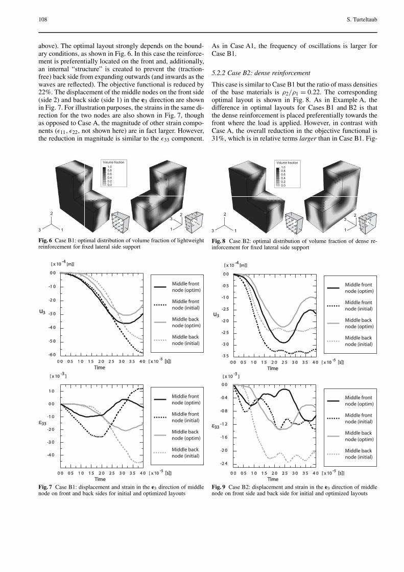
above). The optimal layout strongly depends on the bound-ary conditions, as shown in Fig. 6. In this case the reinforce-ment is preferentially located on the front and, additionally,an internal “structure” is created to prevent the (traction-free) back side from expanding outwards (and inwards as thewaves are reflected). The objective functional is reduced by22%. The displacement of the middle nodes on the front side(side 2) and back side (side 1) in the e3 direction are shownin Fig. 7. For illustration purposes, the strains in the same di-rection for the two nodes are also shown in Fig. 7, thoughas opposed to Case A, the magnitude of other strain compo-nents (ε11, ε22, not shown here) are in fact larger. However,the reduction in magnitude is similar to the ε33 component.

Fig. 6 Case B1: optimal distribution of volume fraction of lightweightreinforcement for fixed lateral side support

Fig. 7 Case B1: displacement and strain in the e3 direction of middlenode on front and back sides for initial and optimized layouts

As in Case A1, the frequency of oscillations is larger forCase B1.

5.2.2 Case B2: dense reinforcement

This case is similar to Case B1 but the ratio of mass densitiesof the base materials is ρ2/ρ1 = 0.22. The correspondingoptimal layout is shown in Fig. 8. As in Example A, thedifference in optimal layouts for Cases B1 and B2 is thatthe dense reinforcement is placed preferentially towards thefront where the load is applied. However, in contrast withCase A, the overall reduction in the objective functional is31%, which is in relative terms larger than in Case B1. Fig-

Fig. 8 Case B2: optimal distribution of volume fraction of dense re-inforcement for fixed lateral side support

Fig. 9 Case B2: displacement and strain in the e3 direction of middlenode on front side and back side for initial and optimized layouts

Optimal non-homogeneous composites for dynamic loading 109

ure 9 shows the change in behavior for the middle nodes onthe front and back side.

6 Performance of optimal designs for different analysistimes

Since the choice of the design time T in the examples shownin the previous section is essentially arbitrary, it is relevantto study the performance of the optimized layouts for timeslarger than T . In particular, it is in principle possible thata material layout that was optimized based on an optimiza-tion interval [0, T ] would provide undesirable results fort > T . In order to obtain some insight into this issue, the per-formance of the optimal layouts in Cases A and B of Sect. 5,which are optimal for the time interval [0, T ], are analyzedfor the time interval [0, 3T ] and, in each case, comparedto the corresponding initial layout. The traction boundaryconditions are extended to the time interval [0, 3T ] as fol-lows:

t(x, t) =

−σ0(2t/T )e3 0 ≤ t ≤ T/2

−σ0e3 T/2 ≤ t ≤ 3Tfor x ∈ S2 ,

Fig. 10 Case A1 (lightweight reinforcement with fixed back side).Above: von Mises stress at the middle node on front side and backside for initial and optimized layouts. Below: Stress energy for initialand optimized layouts

i.e., the traction conditions are the same as for the examplesin Sect. 5 for the time interval [0, T ], while for t > T thetraction on the impacted side is kept constant at its maximumvalue σ0. Moreover, the initial and displacement boundaryconditions are the same as those used in Sect. 5 (i.e., fixedback side for Case A and fixed lateral sides for Case B, asindicated in Table 2).

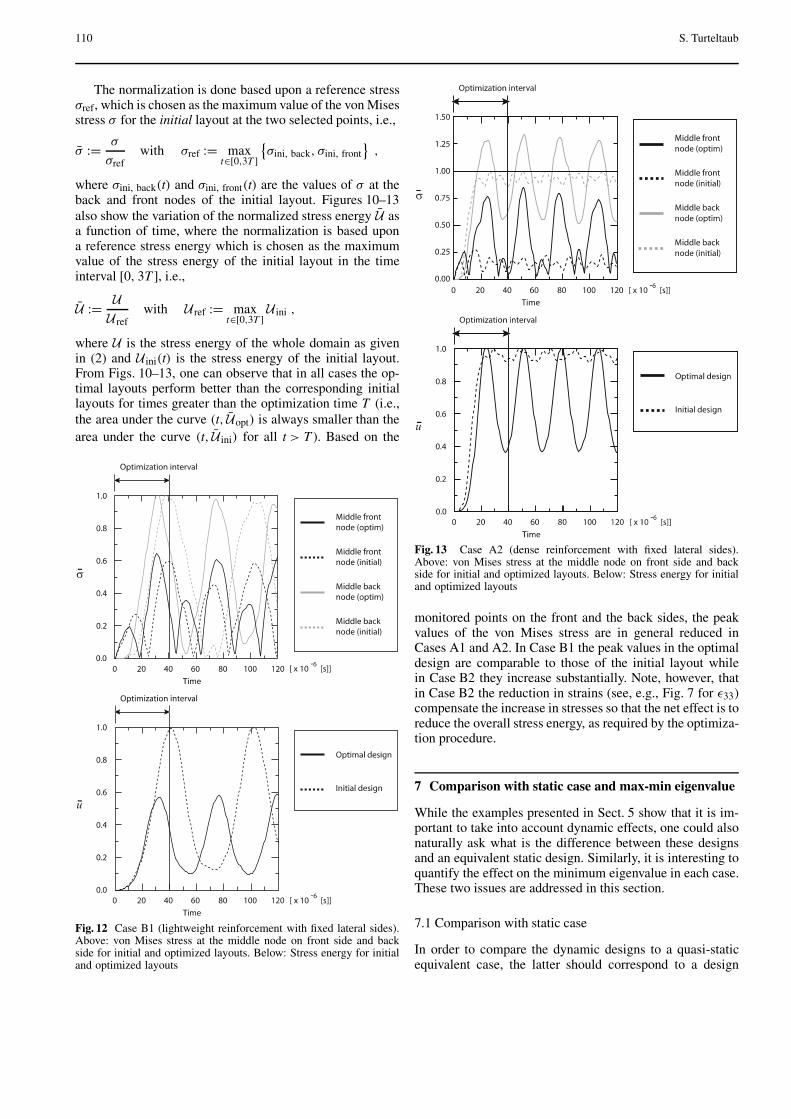
The functional optimized in the foregoing method is thetime average of the stress energy, hence no direct controlis placed upon local values of the stress. As mentioned inthe introduction, the stresses in the optimized layout maybe higher at certain locations compared to the initial lay-out, however this is not a problem per se, since the optimalmaterial at those points is typically different than the initiallayout and it is assumed to have a locally higher resistanceto failure (for example, higher yield stress, higher fracturetoughness, etc.). What is relevant in terms of optimization isthat the overall stress energy, averaged in time, is reduced.Nonetheless, for illustration purposes, the von Mises stressis reported at selected locations in Cases A and B. In particu-lar, the normalized von Mises stress σ at the middle point onside 2 (front of the plate) and side 1 (back of the plate) areshown in Figs 10, 11, 12, 13 for Cases A1, A2, B1 and B2respectively.

Fig. 11 Case A2 (dense reinforcement with fixed back side). Above:von Mises stress at the middle node on front side and back side forinitial and optimized layouts. Below: Stress energy for initial and op-timized layouts

110 S. Turteltaub

The normalization is done based upon a reference stressσref, which is chosen as the maximum value of the von Misesstress σ for the initial layout at the two selected points, i.e.,

σ := σ

σrefwith σref := max

t∈[0,3T ]σini, back, σini, front

,

where σini, back(t) and σini, front(t) are the values of σ at theback and front nodes of the initial layout. Figures 10–13also show the variation of the normalized stress energy U asa function of time, where the normalization is based upona reference stress energy which is chosen as the maximumvalue of the stress energy of the initial layout in the timeinterval [0, 3T ], i.e.,

U := U

U refwith U ref := max

t∈[0,3T ]U ini ,

where U is the stress energy of the whole domain as givenin (2) and U ini(t) is the stress energy of the initial layout.From Figs. 10–13, one can observe that in all cases the op-timal layouts perform better than the corresponding initiallayouts for times greater than the optimization time T (i.e.,the area under the curve (t, Uopt) is always smaller than thearea under the curve (t, U ini) for all t > T ). Based on the

Fig. 12 Case B1 (lightweight reinforcement with fixed lateral sides).Above: von Mises stress at the middle node on front side and backside for initial and optimized layouts. Below: Stress energy for initialand optimized layouts

Fig. 13 Case A2 (dense reinforcement with fixed lateral sides).Above: von Mises stress at the middle node on front side and backside for initial and optimized layouts. Below: Stress energy for initialand optimized layouts

monitored points on the front and the back sides, the peakvalues of the von Mises stress are in general reduced inCases A1 and A2. In Case B1 the peak values in the optimaldesign are comparable to those of the initial layout whilein Case B2 they increase substantially. Note, however, thatin Case B2 the reduction in strains (see, e.g., Fig. 7 for ε33)compensate the increase in stresses so that the net effect is toreduce the overall stress energy, as required by the optimiza-tion procedure.

7 Comparison with static case and max-min eigenvalue

While the examples presented in Sect. 5 show that it is im-portant to take into account dynamic effects, one could alsonaturally ask what is the difference between these designsand an equivalent static design. Similarly, it is interesting toquantify the effect on the minimum eigenvalue in each case.These two issues are addressed in this section.

7.1 Comparison with static case

In order to compare the dynamic designs to a quasi-staticequivalent case, the latter should correspond to a design

Optimal non-homogeneous composites for dynamic loading 111

Fig. 14 Optimal distribution of volume fraction of reinforcement forquasi-static Case A (back side support)

Fig. 15 Optimal distribution of volume fraction of reinforcement forquasi-static Case B (lateral side support)

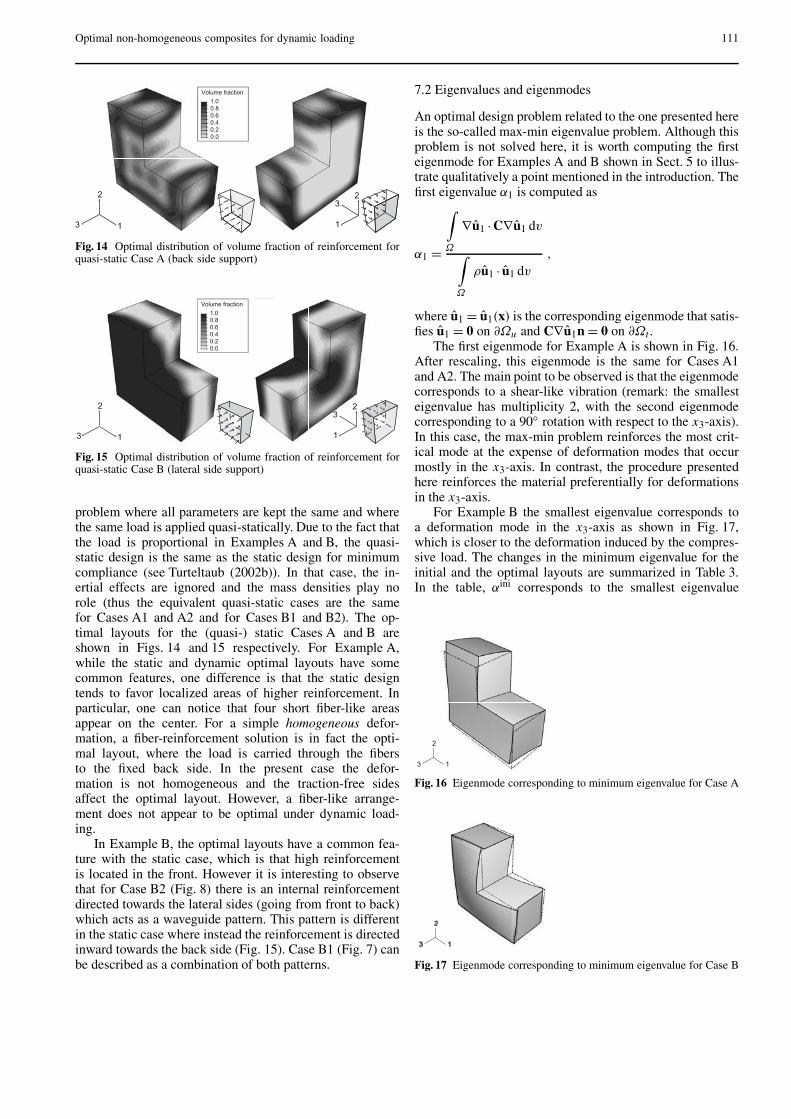
problem where all parameters are kept the same and wherethe same load is applied quasi-statically. Due to the fact thatthe load is proportional in Examples A and B, the quasi-static design is the same as the static design for minimumcompliance (see Turteltaub (2002b)). In that case, the in-ertial effects are ignored and the mass densities play norole (thus the equivalent quasi-static cases are the samefor Cases A1 and A2 and for Cases B1 and B2). The op-timal layouts for the (quasi-) static Cases A and B areshown in Figs. 14 and 15 respectively. For Example A,while the static and dynamic optimal layouts have somecommon features, one difference is that the static designtends to favor localized areas of higher reinforcement. Inparticular, one can notice that four short fiber-like areasappear on the center. For a simple homogeneous defor-mation, a fiber-reinforcement solution is in fact the opti-mal layout, where the load is carried through the fibersto the fixed back side. In the present case the defor-mation is not homogeneous and the traction-free sidesaffect the optimal layout. However, a fiber-like arrange-ment does not appear to be optimal under dynamic load-ing.

In Example B, the optimal layouts have a common fea-ture with the static case, which is that high reinforcementis located in the front. However it is interesting to observethat for Case B2 (Fig. 8) there is an internal reinforcementdirected towards the lateral sides (going from front to back)which acts as a waveguide pattern. This pattern is differentin the static case where instead the reinforcement is directedinward towards the back side (Fig. 15). Case B1 (Fig. 7) canbe described as a combination of both patterns.

7.2 Eigenvalues and eigenmodes

An optimal design problem related to the one presented hereis the so-called max-min eigenvalue problem. Although thisproblem is not solved here, it is worth computing the firsteigenmode for Examples A and B shown in Sect. 5 to illus-trate qualitatively a point mentioned in the introduction. Thefirst eigenvalue α1 is computed as

α1 =

∫

Ω

∇u1 ·C∇u1 dv

∫

Ω

ρu1 · u1 dv

,

where u1 = u1(x) is the corresponding eigenmode that satis-fies u1 = 0 on ∂Ωu and C∇u1n = 0 on ∂Ωt .

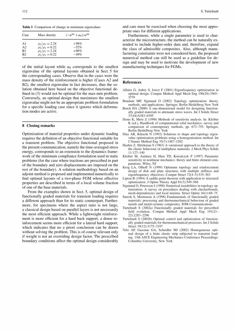
The first eigenmode for Example A is shown in Fig. 16.After rescaling, this eigenmode is the same for Cases A1and A2. The main point to be observed is that the eigenmodecorresponds to a shear-like vibration (remark: the smallesteigenvalue has multiplicity 2, with the second eigenmodecorresponding to a 90 rotation with respect to the x3-axis).In this case, the max-min problem reinforces the most crit-ical mode at the expense of deformation modes that occurmostly in the x3-axis. In contrast, the procedure presentedhere reinforces the material preferentially for deformationsin the x3-axis.

For Example B the smallest eigenvalue corresponds toa deformation mode in the x3-axis as shown in Fig. 17,which is closer to the deformation induced by the compres-sive load. The changes in the minimum eigenvalue for theinitial and the optimal layouts are summarized in Table 3.In the table, αini corresponds to the smallest eigenvalue

Fig. 16 Eigenmode corresponding to minimum eigenvalue for Case A

Fig. 17 Eigenmode corresponding to minimum eigenvalue for Case B

112 S. Turteltaub

Table 3 Comparison of change in minimum eigenvalues

Case Mass density (−αini +α0)/αini

A1 ρ2/ρ1 = 2.24 +98%A2 ρ2/ρ1 = 0.22 −52%B1 ρ2/ρ1 = 2.24 +96%B2 ρ2/ρ1 = 0.22 −49%

of the initial layout while α0 corresponds to the smallesteigenvalue of the optimal layouts obtained in Sect. 5 forthe corresponding cases. Observe that in the cases were themass density of the reinforcement is higher (Cases A2 andB2), the smallest eigenvalue in fact decreases, thus the so-lution obtained here based on the objective functional de-fined in (3) would not be optimal for the max-min problem.Conversely, an optimal design that maximizes the smallesteigenvalue might not be an appropriate problem formulationfor a specific loading case since it ignores which deforma-tion modes are active.

8 Closing remarks

Optimization of material properties under dynamic loadingrequires the definition of an objective functional suitable fora transient problem. The objective functional proposed inthe present communication, namely the time-averaged stressenergy, corresponds to an extension to the dynamics frame-work of the minimum compliance formulation used in staticproblems (for the case where tractions are prescribed in partof the boundary and zero displacements are imposed on therest of the boundary). A solution methodology based on anadjoint method is proposed and implemented numerically tofind optimal layouts of a two-phase FGM whose effectiveproperties are described in terms of a local volume fractionof one of the base materials.

From the examples shown in Sect. 5, optimal design offunctionally graded materials for transient loading requiresa different approach than for its static counterpart. Further-more, for specimens where the aspect ratio is not large,a classical design based on parallel layers is not necessarilythe most efficient approach. While a lightweight reinforce-ment is more efficient for a hard back support, a dense re-inforcement seems more efficient for a lateral hard support,which indicates that no a priori conclusion can be drawnwithout solving the problem. This is of course relevant onlyif weight is not an overriding design factor. The prescribedboundary conditions affect the optimal design considerably

and care must be exercised when choosing the most appro-priate ones for different applications.

Furthermore, while a single parameter is used to char-acterize the microstructure, the method can be naturally ex-tended to include higher-order data and, therefore, expandthe class of admissible composites. Also, although manu-facturing constraints were not considered here, the proposednumerical method can still be used as a guideline for de-sign and may be used to motivate the development of newmanufacturing techniques for FGMs.

References

Allaire G, Aubry S, Jouve F (2001) Eigenfrequency optimization inoptimal design. Comput Method Appl Mech Eng 190(28):3565–3579

Bendsøe MP, Sigmund O (2002) Topology optimization: theory,methods, and applications. Springer, Berlin Heidelberg New York

Bruck HA (2000) A one-dimensional model for designing function-ally graded materials to attenuate stress waves. Int J Solids Struct37(44):6383–6395

Dems K, Mroz Z (1998) Methods of sensitivity analysis. In: KleiberK (ed.), Handbook of computational solid mechanics: survey andcomparison of contemporary methods, pp. 673–755. Springer,Berlin Heidelberg New York

Dıaz AR, Kikuchi N (1992) Solutions to shape and topology eigen-value optimization problems using a homogenization method. IntJ Numer Method Eng 35(7):1487–1502

Hashin Z, Shtrikman S (1963) A variational approach to the theory ofthe elastic behaviour of multiphase materials. J Mech Phys Solids11:127–140

Kleiber M, Antunez H, Hien TD, Kowalczyk P (1997) Parametersensitivity in nonlinear mechanics: theory and finite element com-putations. Wiley, NJ

Krog LA, Olhoff N (1999) Optimum topology and reinforcementdesign of disk and plate structures with multiple stiffness andeigenfrequency objectives. Comput Struct 72(4–5):535–563

Lipton R (1994) A saddle-point theorem with application to structuraloptimization. J Optim Theory Appl 81(3):549–568

Sigmund O, Petersson J (1998) Numerical instabilities in topology op-timization: A survey on procedures dealing with checkerboards,mesh-dependencies and local minima. Struct Optim 16(1):68–75

Suresh S, Mortensen A (1998) Fundamentals of functionally gradedmaterials: processing and thermomechanical behaviour of gradedmetals and metal-ceramic composites. IOM Communications

Turteltaub S (2002a) Functionally graded materials for prescribedfield evolution. Comput Method Appl Mech Eng 191(21–22):2283–2296

Turteltaub S (2002b) Optimal control and optimization of function-ally graded materials for thermomechanical processes. Int J SolidsStruct 39(12):3175–3197

Velo AP, Gazonas GA, Scheidler MJ (2002) Homogeneous opti-mal design of a finite elastic strip subjected to transient load-ing. 15th ASCE Engineering Mechanics Conference Proceedings.Columbia University, New York