This article was downloaded by: [Stony Brook University]On: 24 October 2014, At: 18:56Publisher: Taylor & FrancisInforma Ltd Registered in England and Wales Registered Number: 1072954 Registered office: Mortimer House,37-41 Mortimer Street, London W1T 3JH, UK

Communications in Statistics - Theory and MethodsPublication details, including instructions for authors and subscription information:http://www.tandfonline.com/loi/lsta20

Optimal Spare Ordering Time for PreventiveReplacement to Maximize the Cost EffectivenessJih-An Chen a & Yu-Hung Chien ba Department of Business Administration , Kao-Yuan University , Kaohsiung County, Taiwanb Department of Applied Statistics , National Taichung Institute of Technology , TaichungCity, TaiwanPublished online: 23 Jun 2010.

To cite this article: Jih-An Chen & Yu-Hung Chien (2010) Optimal Spare Ordering Time for Preventive Replacementto Maximize the Cost Effectiveness, Communications in Statistics - Theory and Methods, 39:13, 2404-2421, DOI:10.1080/03610926.2010.484156

To link to this article: http://dx.doi.org/10.1080/03610926.2010.484156

PLEASE SCROLL DOWN FOR ARTICLE

Taylor & Francis makes every effort to ensure the accuracy of all the information (the “Content”) containedin the publications on our platform. However, Taylor & Francis, our agents, and our licensors make norepresentations or warranties whatsoever as to the accuracy, completeness, or suitability for any purpose of theContent. Any opinions and views expressed in this publication are the opinions and views of the authors, andare not the views of or endorsed by Taylor & Francis. The accuracy of the Content should not be relied upon andshould be independently verified with primary sources of information. Taylor and Francis shall not be liable forany losses, actions, claims, proceedings, demands, costs, expenses, damages, and other liabilities whatsoeveror howsoever caused arising directly or indirectly in connection with, in relation to or arising out of the use ofthe Content.

This article may be used for research, teaching, and private study purposes. Any substantial or systematicreproduction, redistribution, reselling, loan, sub-licensing, systematic supply, or distribution in anyform to anyone is expressly forbidden. Terms & Conditions of access and use can be found at http://www.tandfonline.com/page/terms-and-conditions

Communications in Statistics—Theory and Methods, 39: 2404–2421, 2010Copyright © Taylor & Francis Group, LLCISSN: 0361-0926 print/1532-415X onlineDOI: 10.1080/03610926.2010.484156

Optimal Spare Ordering Time for PreventiveReplacement toMaximize the Cost Effectiveness

JIH-AN CHEN1 AND YU-HUNG CHIEN2

1Department of Business Administration, Kao-Yuan University,Kaohsiung County, Taiwan2Department of Applied Statistics, National Taichung Instituteof Technology, Taichung City, Taiwan

This article presents a model for determining the optimal spare ordering time forpreventive replacement under the cost effectiveness criterion. The spare unit forreplacement is available only by order and the lead-time for delivering the sparedue to regular or expedited ordering follows general distributions. To analyze theordering policy, the failure process is modelled by a non homogeneous Poissonprocess. By introducing the ordering, shortage, repair, replacement cost, and thesalvage value, the expected long term cost effectiveness is derived as a criterion ofoptimality. It is shown that, under certain conditions, the optimum spare orderingtime which maximizes the expected cost effectiveness is given by a unique solution ofan equation. A special case of this model is also presented and discussed. Finally,a numerical example is given for illustration of the proposed model.

Keywords Cost effectiveness; Minimal repair; Ordering policy; Preventivereplacement; Salvage; Spare.

Mathematics Subject Classification 90B25; 90B50.

1. Introduction

Most of maintenance policies treated in the literature have assumed implicitly thatat any time there is an unlimited supply of units available for replacement; typicallyspare units are assumed to be inexpensive and bulk purchased under a stockingpolicy (Wang, 2002). However, this might not be true on some occasions. Forinstance, when spare units are expensive and/or storage is costly, it is natural incommercial industries that only one spare unit, which can be delivered by order, isavailable for replacement. In this case, we cannot neglect the random lead-time fordelivering a spare unit. That is, it is essential and practical to introduce the randomlead times. Once we take account of the random lead times, we should consider

Received February 11, 2009; Accepted March 15, 2010Address correspondence to Yu-Hung Chien, Department of Applied Statistics, National

Taichung Institute of Technology, No. 129, Sec. 3, San-min Rd., North District, TaichungCity 40401, Taiwan; E-mail: yhchien@ntit.edu.tw

2404

Dow

nloa

ded

by [

Ston

y B

rook

Uni

vers

ity]

at 1

8:56

24

Oct

ober

201

4

Optimal Spare Ordering Time 2405

an ordering policy that determines when to order a spare and when to replace theoperating unit after it has begun operating.

Previous works on ordering policies have assumed that the costs for preventiveand corrective replacements are equal (Chien, 2005; Dohi et al., 1998; Kaio andOsaki, 1978b,a; Kalpakam and Hameed, 1981; Park and Park, 1979; Sheu, 1999;Sheu and Liou, 1994; Thomas and Osaki, 1978), which implies in essential thatthere is no particular need for preventive replacement. Beside, most of them seek theoptimum ordering policy by minimizing the expected cost per unit time in the longrun as a criterion of optimality. In general, however, the policy maximizing profitrate does not discriminate among large and small investments. Thus, the policy thatmentioned above might have this property. Therefore, the cost effectiveness as analternative criterion is suitable for reflecting efficiency per dollar spent. The costeffectiveness is defined as

s-avaliabilitys-expected cost rate

(where “s-” implies statistical meaning) which reflects the efficiency per dollar outlay.Chien and Chen (2008) and Park and Park (1979) also determined the optimalordering time based on the cost effectiveness criterion, the criterion is useful for theeffective use of available money; especially, this criterion is useful when the benefitsobtained from investment are difficult to quantify. As an example, national securitymay benefit from weapon systems, but expressing the gains in monetary terms isquite challenging (Grant et al., 1982).

In this article, a general failure model with general random repair cost isconsidered, and a spare ordering policy for preventive replacement is presented forsuch a system. In the general failure model, there are two type of failures whenthe system fails. One is Type I failure, which is assumed to be minor and can berectified through minimal repair. The other is Type II failure, which is assumedto be a major failure and can be removed only by replacement. The occurrenceprobability of the Type I or II failures are depend on the system age. Minimalrepair means that the repaired system is returned in the same condition as it was,i.e., the failure rate of the repaired system remains the same as it was just prior tofailure. The minimal repair cost depends on the age and the number of repair, andthe cost for corrective replacement is larger than that for preventive replacement.Salvage value for an un-failed system that preventive replaced should be involvedinto the cost model. The cost effectiveness for operating the system in an infinitetime-span is adopted as a criterion of optimality. The problem is to determine theoptimal scheduled ordering time so as to maximize the expected cost effectiveness.Under some reasonable assumptions, the existence and uniqueness of optimumordering time is derived and discussed. Finally, numerical examples for illustrationthis problem are demonstrated.

The reminder of this article is organized as follows. In Sec. 2, the notations andmodel assumptions about the ordering/replacement model are introduced. In Sec. 3,the mathematical formulation is established. Based on the model, the optimalordering policy is derived, and its structural properties are presented in Sec. 4.A discussion about the special case of this model is given in Sec. 5. Finally,sensitivity analysis is carried out through numerical examples in Sec. 6, and somecomments are also concluded.

Dow

nloa

ded

by [

Ston

y B

rook

Uni

vers

ity]

at 1

8:56

24

Oct

ober

201

4

2406 Chen and Chien

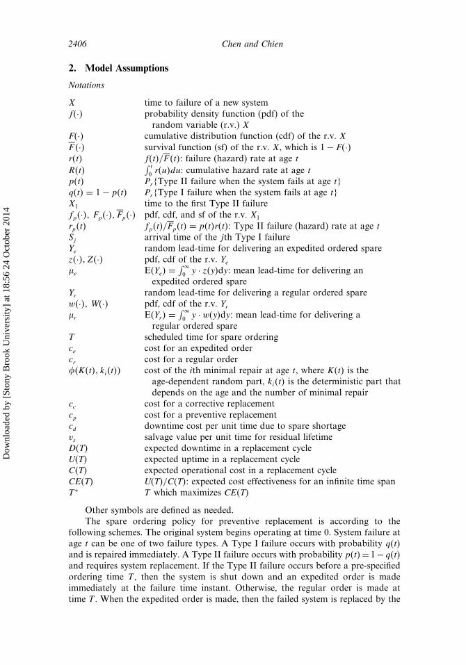
2. Model Assumptions

Notations

X time to failure of a new systemf�·� probability density function (pdf) of the

random variable (r.v.) XF�·� cumulative distribution function (cdf) of the r.v. X�F�·� survival function (sf) of the r.v. X, which is 1− F�·�r�t� f�t�/�F�t�: failure (hazard) rate at age t

R�t�∫ t

0 r�u�du: cumulative hazard rate at age tp�t� Pr{Type II failure when the system fails at age t}q�t� = 1− p�t� Pr{Type I failure when the system fails at age t}X1 time to the first Type II failurefp�·�� Fp�·���Fp�·� pdf, cdf, and sf of the r.v. X1

rp�t� fp�t�/�Fp�t� = p�t�r�t�: Type II failure (hazard) rate at age tSj arrival time of the jth Type I failureYe random lead-time for delivering an expedited ordered sparez�·�� Z�·� pdf, cdf of the r.v. Ye�e E�Ye� =

∫ �0 y · z�y�dy: mean lead-time for delivering an

expedited ordered spareYr random lead-time for delivering a regular ordered sparew�·�� W�·� pdf, cdf of the r.v. Yr�r E�Yr� =

∫ �0 y · w�y�dy: mean lead-time for delivering a

regular ordered spareT scheduled time for spare orderingce cost for an expedited ordercr cost for a regular order��K�t�� ki�t�� cost of the ith minimal repair at age t, where K�t� is the

age-dependent random part, ki�t� is the deterministic part thatdepends on the age and the number of minimal repair

cc cost for a corrective replacementcp cost for a preventive replacementcd downtime cost per unit time due to spare shortagevs salvage value per unit time for residual lifetimeD�T� expected downtime in a replacement cycleU�T� expected uptime in a replacement cycleC�T� expected operational cost in a replacement cycleCE�T� U�T�/C�T�: expected cost effectiveness for an infinite time spanT ∗ T which maximizes CE�T�

Other symbols are defined as needed.The spare ordering policy for preventive replacement is according to the

following schemes. The original system begins operating at time 0. System failure atage t can be one of two failure types. A Type I failure occurs with probability q�t�and is repaired immediately. A Type II failure occurs with probability p�t�= 1− q�t�and requires system replacement. If the Type II failure occurs before a pre-specifiedordering time T , then the system is shut down and an expedited order is madeimmediately at the failure time instant. Otherwise, the regular order is made attime T . When the expedited order is made, then the failed system is replaced by the

Dow

nloa

ded

by [

Ston

y B

rook

Uni

vers

ity]

at 1

8:56

24

Oct

ober

201

4

Optimal Spare Ordering Time 2407

ordered spare as soon as the spare is delivered. The lead time for delivering thatexpedited ordered spare is a generally distributed r.v. with pdf z�t�, cdf Z�t�, andfinite mean �e. When the regular order is made, then the original system, no matteroperating or not, is replaced by the ordered spare as soon as the spare is delivered.The lead time for delivering that regular ordered spare is a generally distributed r.v.with pdf w�t�, cdf W�t�, and finite mean �r , where �r ≥ �e > 0. After a replacement,the procedure is repeated.

Various costs for operating this ordering-replacement procedure are defined asfollows. The cost of the ith minimal repair at age t is ��K�t�� ki�t��, where K�t� is theage-dependent random part, ki�t� is the deterministic part that depends on the ageand the number of minimal repair, and � is a positive non-decreasing continuousfunction. The cost for an expedited order is ce, the cost for a regular order is cr ,and it satisfies ce ≥ cr > 0. The cost for a corrective replacement is cc, the cost fora preventive replacement is cp, and cc ≥ cp > 0 is true. The cost rate resulting fromthe system shutdown is cd. The salvage value per unit time for the residual lifetimeof an un-failed system is vs.

Finally, the following two hypotheses are necessary and required in this study:(i) replacements are made perfectly and do not affect the system’s characteristics;(ii) all failures are instantly detected and is repaired instantaneously if it is a Type Ifailure.

3. Mathematical Formulation

Based on the model assumptions, the mathematical formulation is established in thissection.

3.1. Preliminaries

Suppose the non homogeneous Poisson process (NHPP) �N�t�� t ≥ 0� with intensityr�t� and successive arrival times S1� S2� � � � describes the failure behavior of a system.The two system failure types are associated at random with the event epochs ofthe process. At time Sn, the system has two possible types of failure. The outcomeindicator function is:

n ={0� (Type I failure) with probability q�Sn��

1� (Type II failure) with probability p�Sn��

Let L�t� = ∑N�t�n=1 n count the number of Type II failures of the system in

the interval 0� t�. Then M�t� = N�t�− L�t� counts the number of Type I failures,and it can be shown that �L�t�� t ≥ 0� and �M�t�� t ≥ 0� are independent NHPPswith intensities p�t�r�t� and q�t�r�t� (Savits, 1988). This is similar to the classicaldecomposition of a Poisson process for a constant event probability p. Let X1

denote the waiting time until the first Type II failure, then X1 = inf�t ≥ 0 � L�t� = 1�.Note that X1 is independent of �M�t�� t ≥ 0�. Thus, the sf of the time to first TypeII failure is given by

�Fp�t� = P�X1 > t� = P�L�t� = 0� = exp{−∫ t

0p�x�r�x�dx

}� (1)

In order to develop the model, the following lemma from Sheu and Liou (1994)is required.

Dow

nloa

ded

by [

Ston

y B

rook

Uni

vers

ity]

at 1

8:56

24

Oct

ober

201

4

2408 Chen and Chien

Lemma 3.1. Let �M�t�� t ≥ 0� be a non homogeneous Poisson process with intensityq�t�r�t� and EM�t�� = ∫ t

0 q�x�r�x�dx. Denote the successive arrival time by S1� S2� � � � .Assume that at time Si (i = 1� 2� � � � ) a cost of ��K�Si�� ki�Si�� is incurred. Supposethat K�t� at age t is a random variable with finite mean EK�t��. If �t� is the total costincurred over 0� t�, then

E �t�� = E

[M�t�∑i=1

��K�Si�� ki�Si��

]=

∫ t

0��x�q�x�r�x�dx� (2)

where ��t� = EM�t�EK�t���K�t�� kM�t�+1�t����.

3.2. Model Development

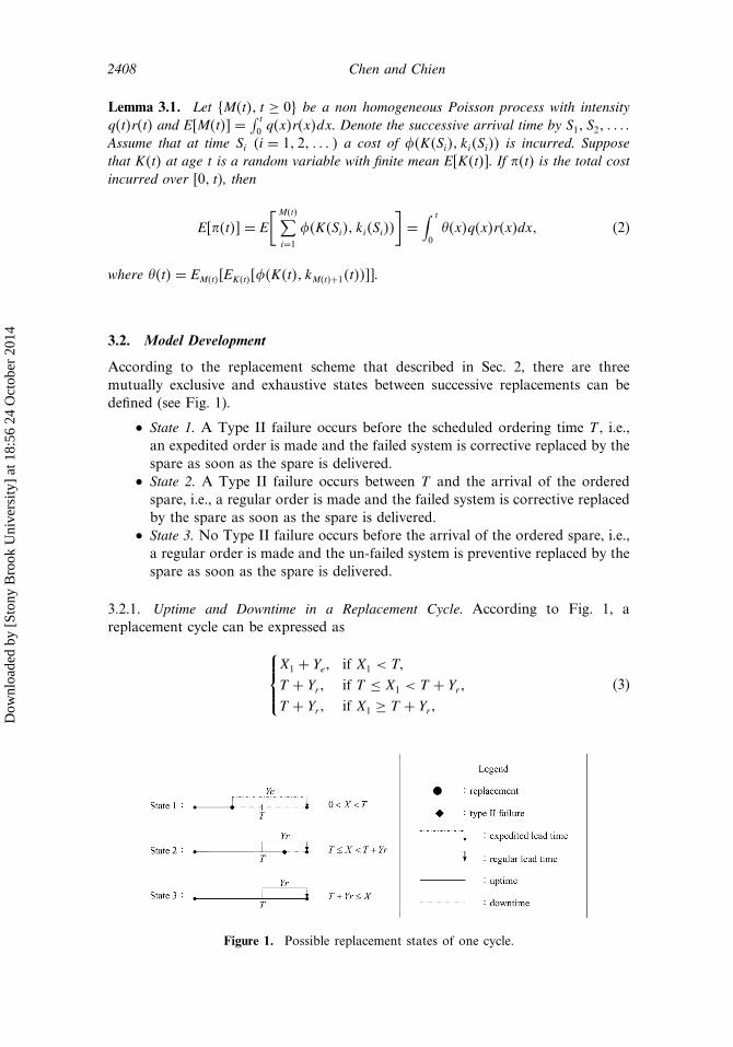
According to the replacement scheme that described in Sec. 2, there are threemutually exclusive and exhaustive states between successive replacements can bedefined (see Fig. 1).

• State 1. A Type II failure occurs before the scheduled ordering time T , i.e.,an expedited order is made and the failed system is corrective replaced by thespare as soon as the spare is delivered.

• State 2. A Type II failure occurs between T and the arrival of the orderedspare, i.e., a regular order is made and the failed system is corrective replacedby the spare as soon as the spare is delivered.

• State 3. No Type II failure occurs before the arrival of the ordered spare, i.e.,a regular order is made and the un-failed system is preventive replaced by thespare as soon as the spare is delivered.

3.2.1. Uptime and Downtime in a Replacement Cycle. According to Fig. 1, areplacement cycle can be expressed as

X1 + Ye� if X1 < T�

T + Yr� if T ≤ X1 < T + Yr�

T + Yr� if X1 ≥ T + Yr�

(3)

Figure 1. Possible replacement states of one cycle.

Dow

nloa

ded

by [

Ston

y B

rook

Uni

vers

ity]

at 1

8:56

24

Oct

ober

201

4

Optimal Spare Ordering Time 2409

where Ye and Yr are the random lead time, respectively, for delivering the expeditedand regular ordered spare. Thus, by Eq. (3), the expected cycle length can beobtained as:

∫ �

0

∫ T

0�x + y�dFp�x�dZ�y�+

∫ �

0

∫ T+y

T�T + y�dFp�x�dW�y�

+∫ �

0

∫ �

T+y�T + y�dFp�x�dW�y�

=∫ �

0

∫ T

0�x + y�dFp�x�dZ�y�+

∫ �

0

∫ �

T�T + y�dFp�x�dW�y�

= �e · Fp�T�+ �r · �Fp�T�+∫ T

0

�Fp�x�dx

= �r − ��r − �e� · Fp�T�+∫ T

0

�Fp�x�dx� (4)

Since downtime only occurs in the states 1 and 2, thus the expected downtimeper cycle is

D�T� =∫ �

0

∫ T

0ydFp�x�dZ�y�+

∫ �

0

∫ T+y

T�T + y − x�dFp�x�dW�y�

=∫ �

0

∫ T+y

TFp�x�dx dW�y�− ��r − �e� · Fp�T�� (5)

Furthermore, since the uptime per cycle is the cycle length minus the downtimeper cycle, thus the expected uptime per cycle can be obtained through Eqs. (4) and(5), which is given by

U�T� = �r +∫ T

0

�Fp�x�dx −∫ �

0

∫ T+y

TFp�x�dx dW�y�

=∫ �

0

∫ T+y

0

�Fp�x�dx dW�y�� (6)

3.2.2. Operational Costs in a Replacement Cycle. The expected operational cost percycle is the sum of the costs for ordering, minimal repair, downtime, replacement,and the salvage value of the system.

Ordering/Downtime Costs: According to Fig. 1, it is obviously that theexpected cost due to spare ordering per cycle is

ce · Fp�T�+ cr · �Fp�T� = cr + �ce − cr�Fp�T�� (7)

and by Eq. (5) the expected cost due to downtime per cycle is

cd ·D�T� = cd

{ ∫ �

0

∫ T+y

TFp�x�dx dW�y�− ��r − �e�Fp�T�

}� (8)

Replacement Costs: Since the replacement that occurs in the states 1 and 2 isthe corrective replacement, and the replacement that occurs in the state 3 is the

Dow

nloa

ded

by [

Ston

y B

rook

Uni

vers

ity]

at 1

8:56

24

Oct

ober

201

4

2410 Chen and Chien

preventive replacement, thus the expected cost due to replacement per cycle is

cc

{Fp�T�+

∫ �

0

∫ T+y

TdFp�x�dW�y�

}+ cp ·

∫ �

0

∫ �

T+ydFp�x�dW�y�

= cp + �cc − cp�∫ �

0Fp�T + y�dW�y�� (9)

Minimal Repair Costs: There are three mutually exclusive and exhaustivepossibilities for the minimal repair costs that exist in every cycle, which can beexpressed as:

M�X1�∑i=1

��K�Si�� ki�Si��� if X1 < T�

M�X1�∑i=1

��K�Si�� ki�Si��� if T ≤ X1 < T + Yr�

M�T+Yr �∑i=1

��K�Si�� ki�Si��� if X1 ≥ T + Yr�

(10)

Thus, by using Lemma 3.1 and take expectation for Eq. (10), the expected cost dueto minimal repair per cycle is

∫ T

0E{M�x�∑

i=1

��K�Si�� ki�Si��

}dFp�x�+

∫ �

0

∫ T+y

TE{M�x�∑

i=1

��K�Si�� ki�Si��

}dFp�x�dW�y�

+∫ �

0

�Fp�T + y�E{M�T+y�∑

i=1

��K�Si�� ki�Si��

}dW�y�

=∫ T

0

∫ x

0��t�q�t�r�t�dtdFp�x�+

∫ �

0

∫ T+y

T

∫ x

0��t�q�t�r�t�dtdFp�x�dW�y�

+∫ �

0

�Fp�T + y�∫ T+y

0��t�q�t�r�t�dtdW�y�

=∫ �

0

∫ T+y

0

�Fp�x���x�q�x�r�x�dx dW�y�� (11)

Salvage Value: It seems reasonable that salvage value of a used unit, whichis still operable, is proportional to the expected residual lifetime (Kaio and Osaki,1978a). Because salvage value only occurs in the state 3, thus the expected salvagevalue per cycle is

vs ·∫ �

0

∫ �

T+y�x − T − y�dFp�x�dW�y� = vs ·

∫ �

0

∫ �

T+y

�Fp�x�dx dW�y�� (12)

Therefore, by Eqs. (7)–(12), the expected operational cost per cycle is

C�T� = �cr + cp�+ �ce − cr�− cd��r − �e��Fp�T�

+∫ �

0

∫ T+y

0

�Fp�x���x�q�x�r�x�dx dW�y�+ �cc − cp�∫ �

0Fp�T + y�dW�y�

+ cd ·∫ �

0

∫ T+y

TFp�x�dx dW�y�− vs ·

∫ �

0

∫ �

T+y

�Fp�x�dx dW�y�� (13)

Dow

nloa

ded

by [

Ston

y B

rook

Uni

vers

ity]

at 1

8:56

24

Oct

ober

201

4

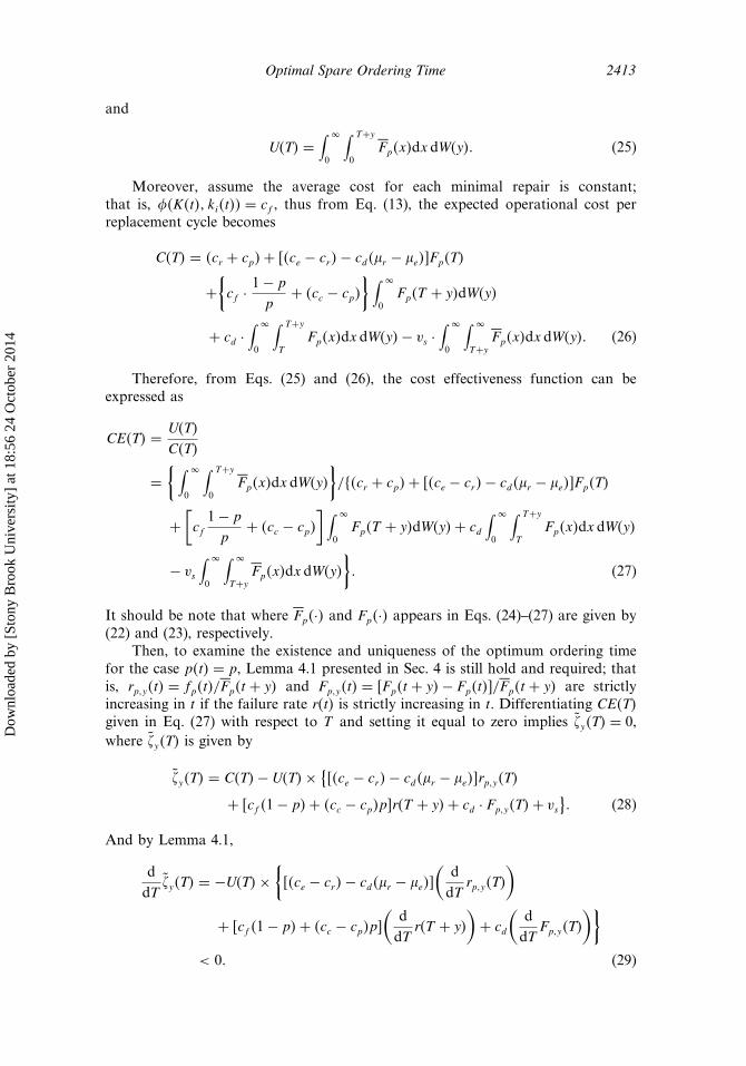
Optimal Spare Ordering Time 2411

3.2.3. The Cost Effectiveness. Since in our formulation for the spare ordering andreplacement process, each replacement is a regeneration point, we can rewrite thecost effectiveness as

s-avaliabilitys-expected cost rate

= expected uptime per cycleexpected operational cost per cycle

�

Therefore, the cost effectiveness function can be expressed as

CE�T� = U�T�

C�T�� (14)

where U�T� and C�T� are, respectively, given by Eqs. (6) and (13).

4. Optimization Analysis

Define rp�y�t� = fp�t�/�Fp�t + y� and Fp�y�t� = Fp�t + y�− Fp�t��/�Fp�t + y�, thefollowing lemma is required and helpful to examine the existence and uniquenessof the optimum ordering policy.

Lemma 4.1. Both rp�y�t� and Fp�y�t� are strictly increasing in t if r�t� is strictlyincreasing in t and p�t� is non decreasing in t.

Proof. Since rp�t� = p�t�r�t� and r�t� have the same monotone properties, strictlyIFR means

rp�t + y�− rp�t� > 0 (15)

and

ddt

rp�t� =ddt fp�t�+ rp�t�fp�t�

�Fp�t�> 0� (16)

which implies

ddt

fp�t�+ rp�t�fp�t� > 0� (17)

Thus, by Eqs. (15) and (17), it yields

ddt

rp�y�t� =ddt fp�t�+ rp�t + y�fp�t�

�Fp�t + y�>

ddt fp�t�+ rp�t�fp�t�

�Fp�t + y�> 0� (18)

On the other hand, by Eq. (15), it yields

ddt

Fp�y�t� =�Fp�t�rp�t + y�− rp�t��

�Fp�t + y�> 0� (19)

Therefore, both rp�y�t� and Fp�y�t� are strictly increasing in t.

Dow

nloa

ded

by [

Ston

y B

rook

Uni

vers

ity]

at 1

8:56

24

Oct

ober

201

4

2412 Chen and Chien

Define the numerator of the derivative of CE�T� in Eq. (14) divided by �Fp�T +y� as �y�T�; that is,

�y�T� = C�T�− U�T�× {�ce − cr�− cd��r − �e��rp�y�T�

+ ��T + y�q�T + y�+ �cc − cp�p�T + y��r�T + y�+ cd · Fp�y�T�+ vs}�(20)

Then, the main results concerning the optimal ordering time T ∗ whichmaximizes CE�T� are summarized below.

Theorem 4.1. Suppose that the function ��t�q�t�+ �cc − cp�p�t��r�t� is continuousand strictly increasing in t, and �ce − cr� ≥ cd��r − �e�. Then:

(i) If �y�0� ≤ 0, then the optimum ordering time T ∗ = 0.(ii) If �y�0� > 0 and �y��� < 0, then there exists a finite and unique optimum ordering

time T ∗ (0 < T ∗ < �) satisfying �y�T∗� = 0.

(iii) If �y��� ≥ 0, then the optimum ordering time T ∗ = �.

where �y�·� is defined in Eq. (20).

Proof. Differentiating CE�T� with respect to T and setting it equal to zero implies�y�T� = 0.

Further,

ddT

�y�T� ≤ −U�T�×{�ce − cr�− cd��r − �e��

(ddT

rp�y�T�

)

+ ddT

���T + y�q�T + y�+ �cc − cp�p�T + y��r�T + y��

+ cd

(ddT

Fp�y�T�

)}< 0 (21)

since both rp�y�t� and Fp�y�t� are strictly increasing in t. Thus, the existence of T ∗ inthe theorem follows trivially.

5. Special Cases

In this section, special cases for the ordering/replacement model are investigated.First, the case p�t� = p is considered. From Eq. (1), the sf of the r.v. X1 becomes

�Fp�t� = exp{−p

∫ t

0r�x�dx

}= �F�t��p� (22)

and the cdf of X1 is

Fp�t� = 1−�Fp�t� = 1− �F�t��p� (23)

Under the case p�t� = p, the expected downtime and uptime in a replacementcycle are as the same forms as Eqs. (5) and (6), respectively, that is,

D�T� =∫ �

0

∫ T+y

TFp�x�dx dW�y�− ��r − �e� · Fp�T�� (24)

Dow

nloa

ded

by [

Ston

y B

rook

Uni

vers

ity]

at 1

8:56

24

Oct

ober

201

4

Optimal Spare Ordering Time 2413

and

U�T� =∫ �

0

∫ T+y

0

�Fp�x�dx dW�y�� (25)

Moreover, assume the average cost for each minimal repair is constant;that is, ��K�t�� ki�t�� = cf , thus from Eq. (13), the expected operational cost perreplacement cycle becomes

C�T� = �cr + cp�+ �ce − cr�− cd��r − �e��Fp�T�

+{cf ·

1− p

p+ �cc − cp�

} ∫ �

0Fp�T + y�dW�y�

+ cd ·∫ �

0

∫ T+y

TFp�x�dx dW�y�− vs ·

∫ �

0

∫ �

T+y

�Fp�x�dx dW�y�� (26)

Therefore, from Eqs. (25) and (26), the cost effectiveness function can beexpressed as

CE�T� = U�T�

C�T�

={ ∫ �

0

∫ T+y

0

�Fp�x�dx dW�y�

}/��cr + cp�+ �ce − cr�− cd��r − �e��Fp�T�

+[cf

1− p

p+ �cc − cp�

] ∫ �

0Fp�T + y�dW�y�+ cd

∫ �

0

∫ T+y

TFp�x�dx dW�y�

− vs

∫ �

0

∫ �

T+y

�Fp�x�dx dW�y�

}� (27)

It should be note that where �Fp�·� and Fp�·� appears in Eqs. (24)–(27) are given by(22) and (23), respectively.

Then, to examine the existence and uniqueness of the optimum ordering timefor the case p�t� = p, Lemma 4.1 presented in Sec. 4 is still hold and required; thatis, rp�y�t� = fp�t�/�Fp�t + y� and Fp�y�t� = Fp�t + y�− Fp�t��/�Fp�t + y� are strictlyincreasing in t if the failure rate r�t� is strictly increasing in t. Differentiating CE�T�given in Eq. (27) with respect to T and setting it equal to zero implies �̃y�T� = 0,where �̃y�T� is given by

�̃y�T� = C�T�− U�T�× {�ce − cr�− cd��r − �e��rp�y�T�

+ cf �1− p�+ �cc − cp�p�r�T + y�+ cd · Fp�y�T�+ vs}� (28)

And by Lemma 4.1,

ddT

�̃y�T� = −U�T�×{�ce − cr�− cd��r − �e��

(ddT

rp�y�T�

)

+ cf �1− p�+ �cc − cp�p�

(ddT

r�T + y�

)+ cd

(ddT

Fp�y�T�

)}< 0� (29)

Dow

nloa

ded

by [

Ston

y B

rook

Uni

vers

ity]

at 1

8:56

24

Oct

ober

201

4

2414 Chen and Chien

Thus, the properties related to the optimal ordering time T ∗ which maximizes theCE�T� given in (27) are summarized below.

Corollary 5.1. Suppose �ce − cr� ≥ cd��r − �e�.

(i) If �̃y�0� ≤ 0, then the optimum ordering time T ∗ = 0.(ii) If �̃y�0� > 0 and �̃y��� < 0, then there exists a finite and unique optimum ordering

time T ∗ (0 < T ∗ < �) satisfying �̃y�T∗� = 0.

(iii) If �̃y��� ≥ 0, then the optimum ordering time T ∗ = �.

where �̃y�·� is defined in Eq. (28).

Furthermore, a constant lead time for delivering the ordered spare is considered.That is, assume that the lead-time for delivering an expedited ordered spare is �e,and the lead-time for delivering an regular ordered spare is �r . Thus, from Eqs. (24)and (25), the expected downtime and uptime in a replacement cycle become

D�T� =∫ T+�r

TFp�x�dx − ��r − �e� · Fp�T�� (30)

and

U�T� =∫ T+�r

0

�Fp�x�dx� (31)

and form Eq. (26), the expected operational cost per replacement cycle becomes

C�T� = �cr + cp�+ �ce − cr�− cd��r − �e��Fp�T�+{cf ·

1− p

p+ �cc − cp�

}Fp�T + y�

+cd ·∫ T+�r

TFp�x�dx − vs ·

∫ �

T+�r

�Fp�x�dx� (32)

Therefore, by Eqs. (31) and (32), the cost effectiveness function under theconstant delivery lead time is

CE�T� = U�T�

C�T�

={ ∫ T+�r

0

�Fp�x�dx}/{

�cr + cp�+ �ce − cr�− cd��r − �e��Fp�T�

+{cf ·

1− p

p+ �cc − cp�

}Fp�T + y�+ cd ·

∫ T+�r

TFp�x�dx

− vs ·∫ �

T+�r

�Fp�x�dx}� (33)

ddT CE�T� = 0 is equivalent to

��r �T� = C�T�− U�T�× {�ce − cr�− cd��r − �e��rp��r �T�

+ cf �1− p�+ �cc − cp�p�r�T + �r�+ cd · Fp��r�T�+ vs

}= 0� (34)

Dow

nloa

ded

by [

Ston

y B

rook

Uni

vers

ity]

at 1

8:56

24

Oct

ober

201

4

Optimal Spare Ordering Time 2415

where rp� �r �t� = fp�t�/�Fp�t + �r�, Fp��r�t� = Fp�t + �r�− Fp�t��/�Fp�t + �r�. By

Lemma 4.1, both rp��r �t� and Fp��r�t� are strictly increasing in t if r�t� is strictly

increasing in t, thus ddT ��r �T� < 0 is hold.

Then, the properties related to the optimal ordering time T ∗ which maximizesthe CE�T� given in (33) are summarized below.

Corollary 5.2. Suppose �ce − cr� ≥ cd��r − �e�.

(i) If ��r �0� ≤ 0, then the optimum ordering time T ∗ = 0.(ii) If ��r �0� > 0 and ��r ��� < 0, then there exists a finite and unique optimum ordering

time T ∗ (0 < T ∗ < �) satisfying ��r �T∗� = 0.

(iii) If ��r ��� ≥ 0, then the optimum ordering time T ∗ = �.

where ��r �·� is defined in Eq. (34).

Based on Theorem 4.1, as well as the Corollaries 5.1 and 5.2, the followingremarks can be drawn.

Remark 5.1. For both the general case and special cases, the properties of theoptimal spare ordering policy are very similarly. T ∗ = 0 means that the optimalspare ordering policy is to place a regular order at the same instant when a newsystem is put in service and never place an expedited order; while T ∗ = � meansthe optimal policy is to place an expedited order at the instant of the Type II failureand never place a regular order.

Remark 5.2. A sufficient condition for the optimality in the theorem andcorollaries, �ce − cr� ≥ cd��r − �e�, has been widely used in spare ordering policies(Chien, 2005; Dohi et al., 1998; Kaio and Osaki, 1978a,b; Kalpakam and Hameed,1981; Sheu, 1999; Sheu and Liou, 1994). However it should be noted that theassumption does not economically justify placing an expedited order since theadditional cost for the expedition �ce − cr� is larger than the savings obtained fromthe expedition cd��r − �e�. Hence, it is meaningful only when there exists suchintangibles as loss of goodwill, reputation, and credit which are difficult to bequantified and included in downtime cost.

Remark 5.3. The condition �y�0� ≤ 0 in Theorem 4.1 is equivalent to

C�0�U�0�

≤ [�ce − cr�− cd��r − �e�

]rp�y�0�+ ��y�q�y�+ �cc − cp�p�y��r�y�

+ cd · Fp�y�0�+ vs� (35)

The right-hand side of the above inequality can be represented as the expectedmarginal operational cost at any time y the spare arrives when it is regular orderedat time 0, where C�0�/U�0� is the expected operational cost per unit up-time whenthe spare is regular ordered at time 0. This means that if the spare is regularordered at time 0 and the operational cost per unit uptime is less than the marginaloperational cost at any time the ordered spare arrives, then the optimal spareordering policy is always to place an order for a spare at time 0, i.e., place a regularorder at the same instant when a new system is put in service and never place anexpedited order. Similar properties can also be found in Corollaries 5.1 and 5.2.

Dow

nloa

ded

by [

Ston

y B

rook

Uni

vers

ity]

at 1

8:56

24

Oct

ober

201

4

2416 Chen and Chien

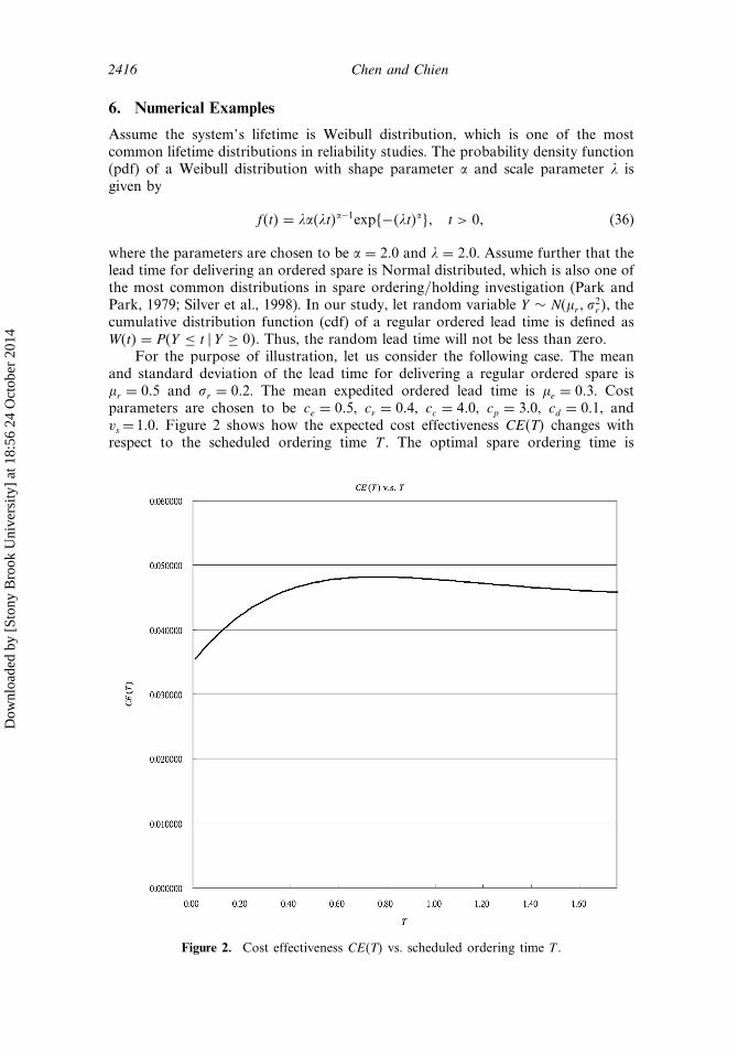
6. Numerical Examples

Assume the system’s lifetime is Weibull distribution, which is one of the mostcommon lifetime distributions in reliability studies. The probability density function(pdf) of a Weibull distribution with shape parameter � and scale parameter � isgiven by

f�t� = ����t��−1exp�−��t���� t > 0� (36)

where the parameters are chosen to be � = 2�0 and � = 2�0. Assume further that thelead time for delivering an ordered spare is Normal distributed, which is also one ofthe most common distributions in spare ordering/holding investigation (Park andPark, 1979; Silver et al., 1998). In our study, let random variable Y ∼ N��r� �

2r �, the

cumulative distribution function (cdf) of a regular ordered lead time is defined asW�t� = P�Y ≤ t � Y ≥ 0�. Thus, the random lead time will not be less than zero.

For the purpose of illustration, let us consider the following case. The meanand standard deviation of the lead time for delivering a regular ordered spare is�r = 0�5 and �r = 0�2. The mean expedited ordered lead time is �e = 0�3. Costparameters are chosen to be ce = 0�5, cr = 0�4, cc = 4�0, cp = 3�0, cd = 0�1, andvs = 1�0. Figure 2 shows how the expected cost effectiveness CE�T� changes withrespect to the scheduled ordering time T . The optimal spare ordering time is

Figure 2. Cost effectiveness CE�T� vs. scheduled ordering time T .

Dow

nloa

ded

by [

Ston

y B

rook

Uni

vers

ity]

at 1

8:56

24

Oct

ober

201

4

Optimal Spare Ordering Time 2417

Table 1Optimal policies under variousce based on parameters cr = 0�4,

cc = 4�0, cp = 3�0, cd = 0�1,vs = 1�0 are fixed

ce T ∗ CE�T ∗�

0.5 0.76 0.0481891.0 0.70 0.0477961.5 0.66 0.0474702.0 0.63 0.0471882.5 0.60 0.0469393.0 0.58 0.0467163.5 0.56 0.0465134.0 0.55 0.0463274.5 0.53 0.046155

determined by maximizing the expected cost effectiveness. Under this case, theoptimal policy is placing a regular order at T ∗ = 0�76 and the corresponding costeffectiveness is CE�T ∗� = 0�0482.

Furthermore, to investigate the effect of �r on the ordering policy, we haveobtained the following by numerical methods. For �r = 0�01, 0.05, 0.10, 0.15, 0.20,the optimal spare ordering times maximizing the cost effectiveness are 0.71, 0.71,0.72, 0.74, 0.76, respectively; the corresponding cost effectiveness are 0.048674,0.048645, 0.048554, 0.048392, 0.048189, respectively. As might be expected, as thestandard deviation �r increases, the optimal cost effectiveness decreases due touncertainty; but, the corresponding optimal ordering time increases, according as �r

increases. This is reasonable and confirms to our expectation since more stabilize of

Table 2Optimal policies under variouscr based on parameters ce = 0�5,

cc = 4�0, cp = 3�0, cd = 0�1,vs = 1�0 are fixed

cr T ∗ CE�T ∗�

0.05 0.65 0.0509480.10 0.66 0.0505150.15 0.68 0.0500970.20 0.69 0.0496910.25 0.71 0.0492970.30 0.73 0.0489160.35 0.74 0.0485470.40 0.76 0.0481890.45 0.78 0.047843

Dow

nloa

ded

by [

Ston

y B

rook

Uni

vers

ity]

at 1

8:56

24

Oct

ober

201

4

2418 Chen and Chien

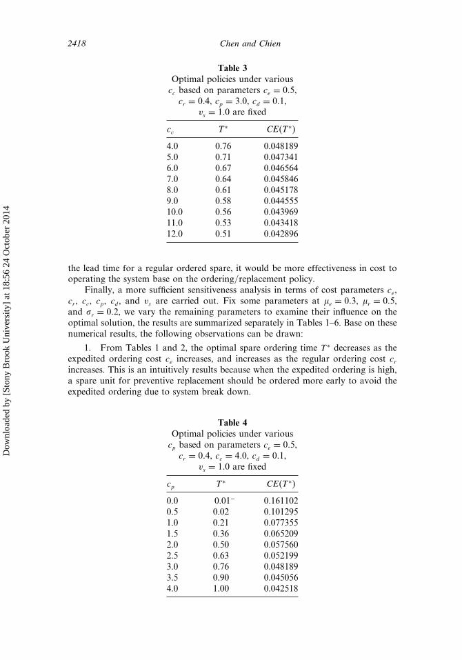
Table 3Optimal policies under variouscc based on parameters ce = 0�5,

cr = 0�4, cp = 3�0, cd = 0�1,vs = 1�0 are fixed

cc T ∗ CE�T ∗�

4.0 0.76 0.0481895.0 0.71 0.0473416.0 0.67 0.0465647.0 0.64 0.0458468.0 0.61 0.0451789.0 0.58 0.04455510.0 0.56 0.04396911.0 0.53 0.04341812.0 0.51 0.042896

the lead time for a regular ordered spare, it would be more effectiveness in cost tooperating the system base on the ordering/replacement policy.

Finally, a more sufficient sensitiveness analysis in terms of cost parameters ce,cr , cc, cp, cd, and vs are carried out. Fix some parameters at �e = 0�3, �r = 0�5,and �r = 0�2, we vary the remaining parameters to examine their influence on theoptimal solution, the results are summarized separately in Tables 1–6. Base on thesenumerical results, the following observations can be drawn:

1. From Tables 1 and 2, the optimal spare ordering time T ∗ decreases as theexpedited ordering cost ce increases, and increases as the regular ordering cost crincreases. This is an intuitively results because when the expedited ordering is high,a spare unit for preventive replacement should be ordered more early to avoid theexpedited ordering due to system break down.

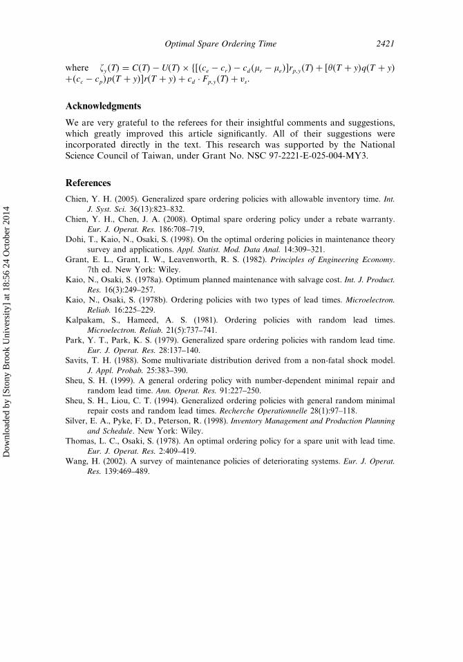
Table 4Optimal policies under variouscp based on parameters ce = 0�5,

cr = 0�4, cc = 4�0, cd = 0�1,vs = 1�0 are fixed

cp T ∗ CE�T ∗�

0.0 0.01− 0.1611020.5 0.02 0.1012951.0 0.21 0.0773551.5 0.36 0.0652092.0 0.50 0.0575602.5 0.63 0.0521993.0 0.76 0.0481893.5 0.90 0.0450564.0 1.00 0.042518

Dow

nloa

ded

by [

Ston

y B

rook

Uni

vers

ity]

at 1

8:56

24

Oct

ober

201

4

Optimal Spare Ordering Time 2419

Table 5Optimal policies under variouscd based on parameters ce = 0�5,

cr = 0�4, cc = 4�0, cp = 3�0,vs = 1�0 are fixed

cd T ∗ CE�T ∗�

0.05 0.77 0.0482490.10 0.76 0.0481890.15 0.76 0.0481290.20 0.75 0.0480710.25 0.74 0.0480130.30 0.74 0.0479560.35 0.73 0.0478990.40 0.73 0.0478430.45 0.72 0.047788

2. From Tables 3 and 4, the optimal spare ordering time T ∗ decreases as thecorrective replacement cost cc increases, and increases as the preventive replacementcost cp increases. This is to be expected because when the cost for a failurereplacement is high, one should order a spare more early for preventive replacementto avoid system failures. Conversely, when the cost for a preventive replacement ishigh, one should wait as long as possible before ordering a spare.

3. From Table 5, as the downtime cost cd increases, the optimal spare orderingtime T ∗ decreases. The reason is that when a system with higher downtime cost, aspare unit for preventive replacement should be ordered more early to avoid systemshut down.

Table 6Optimal policies under various vsbased on parameters ce = 0�5,cr = 0�4, cc = 4�0, cp = 3�0,

cd = 0�1 are fixed

vs T ∗ CE�T ∗�

1.0 0.76 0.0481892.0 0.68 0.0488713.0 0.59 0.0497414.0 0.50 0.0508705.0 0.40 0.0523746.0 0.29 0.0544597.0 0.16 0.0575478.0 0.01 0.0627279.0 0.01− 0.070475

Dow

nloa

ded

by [

Ston

y B

rook

Uni

vers

ity]

at 1

8:56

24

Oct

ober

201

4

2420 Chen and Chien

4. From Table 6, as the salvage value vs increases, the optimal spare orderingtime T ∗ decreases. This is also reasonable because when the salvage value is large,one should order a spare more early for preventive replacement in order to get thebenefits from that un-failed unit.

5. From Tables 1–6, as might be expected, the optimal expected costeffectiveness decreases as the ordering, replacement or downtime costs increases, andincreases as the salvage value increases.

All the numerical results are intuitive and match our expectations.

Appendix: Derivation of Eq. (20)

By Eqs. (6), (13), and (14), the numerator of the derivative of CE�T� is

C�T�× U ′�T�− U�T�× C ′�T�

= C�T�×∫ �

0

�Fp�T + y�dW�y�− U�T�×{�ce − cr�− cd��r − �e��fp�T�

+∫ �

0

�Fp�T + y���T + y�q�T + y�r�T + y�dW�y�+ �cc − cp�∫ �

0fp�T + y�dW�y�

+ cd

∫ �

0Fp�T + y�− Fp�T��dW�y�+ vs

∫ �

0

�Fp�T + y�dW�y�

}

= C�T�×∫ �

0

�Fp�T + y�dW�y�− U�T�×∫ �

0

{�ce − cr�− cd��r − �e��fp�T�

+�Fp�T + y���T + y�q�T + y�r�T + y�+ �cc − cp�fp�T + y�

+ cdFp�T + y�− Fp�T��+ vs�Fp�T + y�

}dW�y�

= C�T�×∫ �

0

�Fp�T + y�dW�y�−∫ �

0

�Fp�T + y�U�T�

{�ce − cr�− cd��r − �e��

× fp�T�

�Fp�T + y�+ ��T + y�q�T + y�r�T + y�+ �cc − cp�

fp�T + y�

�Fp�T + y�

+ cdFp�T + y�− Fp�T�

�Fp�T + y�+ vs

}dW�y�

=∫ �

0C�T��Fp�T + y�dW�y�−

∫ �

0

�Fp�T + y�U�T�{�ce − cr�− cd��r − �e��rp�y�T�

+ ��T + y�q�T + y�r�T + y�+ �cc − cp�p�T + y�r�T + y�+ cdFp�y�T�+ vs}dW�y�

=∫ �

0C�T��Fp�T + y�dW�y�−

∫ �

0

�Fp�T + y�U�T�{�ce − cr�− cd��r − �e��rp�y�T�

+ ��T + y�q�T + y�+ �cc − cp�p�T + y��r�T + y�+ cdFp�y�T�+ vs}dW�y�

=∫ �

0

�Fp�T + y�{C�T�− U�T�× {

�ce − cr�− cd��r − �e��rp�y�T�++ ��T + y�q�T + y�+ �cc − cp�p�T + y��r�T + y�+ cd · Fp�y�T�+ vs

}}dW�y�

=∫ �

0

�Fp�T + y��y�T�dW�y��

Dow

nloa

ded

by [

Ston

y B

rook

Uni

vers

ity]

at 1

8:56

24

Oct

ober

201

4

Optimal Spare Ordering Time 2421

where �y�T� = C�T�− U�T�× ��ce − cr�− cd��r − �e��rp�y�T�+ ��T + y�q�T + y�+�cc − cp�p�T + y��r�T + y�+ cd · Fp�y�T�+ vs.

Acknowledgments

We are very grateful to the referees for their insightful comments and suggestions,which greatly improved this article significantly. All of their suggestions wereincorporated directly in the text. This research was supported by the NationalScience Council of Taiwan, under Grant No. NSC 97-2221-E-025-004-MY3.

References

Chien, Y. H. (2005). Generalized spare ordering policies with allowable inventory time. Int.J. Syst. Sci. 36(13):823–832.

Chien, Y. H., Chen, J. A. (2008). Optimal spare ordering policy under a rebate warranty.Eur. J. Operat. Res. 186:708–719,

Dohi, T., Kaio, N., Osaki, S. (1998). On the optimal ordering policies in maintenance theorysurvey and applications. Appl. Statist. Mod. Data Anal. 14:309–321.

Grant, E. L., Grant, I. W., Leavenworth, R. S. (1982). Principles of Engineering Economy.7th ed. New York: Wiley.

Kaio, N., Osaki, S. (1978a). Optimum planned maintenance with salvage cost. Int. J. Product.Res. 16(3):249–257.

Kaio, N., Osaki, S. (1978b). Ordering policies with two types of lead times. Microelectron.Reliab. 16:225–229.

Kalpakam, S., Hameed, A. S. (1981). Ordering policies with random lead times.Microelectron. Reliab. 21(5):737–741.

Park, Y. T., Park, K. S. (1979). Generalized spare ordering policies with random lead time.Eur. J. Operat. Res. 28:137–140.

Savits, T. H. (1988). Some multivariate distribution derived from a non-fatal shock model.J. Appl. Probab. 25:383–390.

Sheu, S. H. (1999). A general ordering policy with number-dependent minimal repair andrandom lead time. Ann. Operat. Res. 91:227–250.

Sheu, S. H., Liou, C. T. (1994). Generalized ordering policies with general random minimalrepair costs and random lead times. Recherche Operationnelle 28(1):97–118.

Silver, E. A., Pyke, F. D., Peterson, R. (1998). Inventory Management and Production Planningand Schedule. New York: Wiley.

Thomas, L. C., Osaki, S. (1978). An optimal ordering policy for a spare unit with lead time.Eur. J. Operat. Res. 2:409–419.

Wang, H. (2002). A survey of maintenance policies of deteriorating systems. Eur. J. Operat.Res. 139:469–489.

Dow

nloa

ded

by [

Ston

y B

rook

Uni

vers

ity]

at 1

8:56

24

Oct

ober

201

4