Embed Size (px)
Citation preview
HAL Id: tel-01417133https://tel.archives-ouvertes.fr/tel-01417133
Submitted on 15 Dec 2016
HAL is a multi-disciplinary open accessarchive for the deposit and dissemination of sci-entific research documents, whether they are pub-lished or not. The documents may come fromteaching and research institutions in France orabroad, or from public or private research centers.
L’archive ouverte pluridisciplinaire HAL, estdestinée au dépôt et à la diffusion de documentsscientifiques de niveau recherche, publiés ou non,émanant des établissements d’enseignement et derecherche français ou étrangers, des laboratoirespublics ou privés.
Optimal sizing and control of energy storage systems forthe electricity markets participation of intelligent
photovoltaic power plantsAndoni Saez de Ibarra Martinez de Contrasta
To cite this version:Andoni Saez de Ibarra Martinez de Contrasta. Optimal sizing and control of energy storage sys-tems for the electricity markets participation of intelligent photovoltaic power plants. Electric power.Université Grenoble Alpes, 2016. English. �NNT : 2016GREAT057�. �tel-01417133�

THÈSEPour obtenir le grade de
DOCTEUR DE LA COMMUNAUTE UNIVERSITE GRENOBLE ALPESSpécialité : Génie Electrique
Arrêté ministériel : 7 août 2006
Présentée par
Andoni SAEZ DE IBARRA MARTINEZ DE CONTRASTA
Thèse dirigée par Seddik BACHA etcodirigée par Vincent DEBUSSCHERE et Aitor MILO
préparée au sein du Laboratoire de Génie Electrique de Grenoble(G2Elab) et IK4-IKERLAN Technology Research Centredans l'École Doctorale Électronique, Électrotechnique, Automatique & Traitement du Signal (EEATS)
Dimensionnement et contrôle-commande optimisé des systèmes de stockage énergétique pour la participation au marché de l'électricité des parcs photovoltaïques intelligentsThèse soutenue publiquement le 7 octobre 2016,devant le jury composé de :
M. Cristian NICHITAProfesseur à l’Université Le Havre, Président
M. Bruno BURGERFraunhofer ISE, Rapporteur
M. Luis MARTINEZ SALAMEROProfesseur à l’Universitat Rovira i Virgili, Rapporteur
M. Ionel VECHIUProfesseur à l’ESTIA, Rapporteur
M. Seddik BACHAProfesseur à l’Université Grenoble Alpes, Directeur de thèse
M. Vincent DEBUSSCHEREMaître de Conférences Grenoble INP, Co-encadrant de thèse
M. Aitor MILOIK4-IKERLAN Technology Research Centre, Co-encadrant de thèse
Mme. Haizea GAZTAÑAGAIK4-IKERLAN Technology Research Centre, Examinatrice
M. Tuan TRAN QUOCCEA-INES, Invité


Résumé
iii
Titre : Dimensionnement et contrôle-commande optimisé des systèmes de stockage
énergétique pour la participation au marché de l'électricité des parcs photovoltaïques
intelligents
Résumé
L’objet de cette thèse est l’intégration des parcs photovoltaïques intelligents au marché
de l’électricité dans un environnement de libre concurrence. Les centrales photovoltaïques
intelligentes sont celles qu’incluent systèmes de stockage pour réduire sa variabilité et en
plus fournir à l’ensemble une plus grande contrôlabilité. Ces objectives techniques sont
obtenues grâce à la capacité bidirectionnelle d’échange et stockage d’énergie qu’apportent
les systèmes de stockage, dans ce cas, les batteries. Pour obtenir la rentabilité maximale des
systèmes de stockage, le dimensionnement doit être optimisé en même temps que la
stratégie de gestion avec laquelle le système de stockage est commandé. Dans cette thèse,
une fois la technologie de stockage plus adapté à l’application photovoltaïque est
sélectionnée, à savoir la technologie de lithium-ion, une participation innovatrice de part des
parcs photovoltaïques intelligents dans le marché de l’électricité est proposée qui optimise à
la fois le dimensionnement et la stratégie de gestion d’une manière simultanée. Ce
processus d'optimisation ainsi que la participation au marché de l'électricité a été appliquée
dans un cas d’étude réel, ce qui confirme que cette procédure permet de maximiser la
rentabilité économique de ce type de production.
Mots clés : centrale photovoltaïque, system de stockage d’énergie, réseau, optimisation,
marché de l’électricité, dimensionnement, stratégie de contrôle-commande.
Title: Optimal sizing and control of energy storage systems for the electricity markets
participation of intelligent photovoltaic power plants
Abstract
The present PhD deals with the integration of intelligent photovoltaic (IPV) power plants
in the electricity markets in an environment subject to free competition. The IPV power
plants are those that include energy storage systems to reduce the variability and to provide
the entire group a controllability increase. These technical objectives are obtained thanks to
the bidirectional exchanging and storing capability that the storage system contributes to, in
this case, battery energy storage system (BESS). In order to obtain the maximum profitability
of the BESS, the sizing must be optimized together with the control strategy that the BESS
will be operated with. In the present PhD, once the most performing battery energy storage
technology has been selected, the lithium-ion technology, an innovative IPV power plant
electricity market participation process is proposed which optimizes both the sizing and the
energy management strategy in the same optimization step. This optimization process
together with the electricity market participation has been applied in a real case study,
confirming that this procedure permits to maximize the economic profitability of this type of
generation.
Keywords: photovoltaic power plant, energy storage system, grid, optimization,
electricity markets, sizing, energy management strategy.

Resumen
iv
Título: Dimensionamiento y control óptimos de sistemas de almacenamiento para la
participación en los mercados eléctricos de plantas fotovoltaicas inteligentes
Resumen
Esta tesis se centra en la integración de las plantas fotovoltaicas inteligentes en los
mercados eléctricos en un entorno de libre competencia. Las plantas fotovoltaicas
inteligentes son las que incluyen sistemas de almacenamiento para reducir su variabilidad y
dotar al conjunto de una mayor controlabilidad. Estos objetivos técnicos se obtienen gracias
a la capacidad bidireccional de intercambio y al almacenamiento de energía que aporta el
sistema de almacenamiento, en este caso, baterías. Para obtener la máxima rentabilidad de
los sistemas de almacenamiento se tiene que optimizar el dimensionamiento junto con la
estrategia de gestión con la que se opere dicha batería. En esta tesis, tras determinar la
tecnología de almacenamiento más adecuada para esta aplicación, la tecnología de litio-ion,
se ha propuesto una innovadora participación en los mercados eléctricos por parte de las
plantas fotovoltaicas inteligentes, la cual optimiza tanto su gestión como su
dimensionamiento de manera conjunta. Este proceso de optimización junto con la
participación en los mercados eléctricos ha sido aplicado en un caso de estudio real,
confirmando que este procedimiento permite maximizar la rentabilidad económica de este
tipo de generadores.
Palabras clave: parque fotovoltaico, sistema de almacenamiento, red, optimización,
mercado eléctrico, dimensionamiento, estrategia de gestión energética.
Izenburua: Biltegiratze sistemen dimentsionamendu eta kontrol optimoak parke
fotoboltaiko adimenduek elektrizitate-merkatuetan parte-hartzeko.
Laburpena
Tesi hau parke fotoboltaiko adimenduen integrazioan oinarritzen da, merkatu
elektrikoetan parte hartu ahal izateko konpetentzia libreko inguru batean. Parke
fotoboltaiko adimenduak biltegiratze sistemak barneratzen dituztenak dira, euren
aldagarritasuna murrizteko eta talde osoari kontrolagarritasun handiagoa emateko. Helburu
tekniko hauek potentzi aldaketa bidirekzionalari esker lortzen dira eta baita biltegiratze
sistemetan gordeta dagoen energiari esker, kasu honetan, baterietan dagoen energiari
esker. Biltegiratze sistemen errentagarritasun handiena lortzeko, bateriaren
dimentsionamendua optimizatu behar da bere kudeaketa estrategiarekin batera. Tesi
honetan, behin biltegiratze teknologia hoberena aukeratu ondoren, litio ioizko teknologia,
parke fotoboltaiko adimenduaren aldetik elektrizitate merkatuan parte hartzeko estrategia
berritzaile bat proposatu da, bai bere kudeaketa eta baita bere dimentsionamendua aldi
berean optimizatuz. Optimizazio prozesu hau, merkatu parte-hartzearekin batera azterketa
kasu erreal batean aplikatu izan da, prozesu hau sorgailu mota hauen errentagarritasun
ekonomikoa maximizatzeko aukera ematen duela baieztatuz.
Hitz gakoak: parke fotoboltaikoa, biltegiratze sistema, sare elektrikoa, optimizazioa,
merkatu elektrikoa, dimentsionamendua, kudeaketa energetikoko estrategia.

When you talk, you are only repeating what you know; but
when you listen, you learn something new.
-Dalai Lama-


Acknowledgements
vii
Acknowledgements
I want to tell a story that started eight years ago, when I was in the third course of the
electrical engineering in Mondragon University when the professor Cecilio Ugarte offered to
me the possibility to complete my engineering studies both in ENSEEIHT of Toulouse and in
ENSE3 of Grenoble. After having correctly chosen to come to the university where I have
already completed 6 years of different studies (engineering and PhD thesis), I prepared my
bag plenty of wishes for knowing another culture and for learning different things as
technical skills from very distinguished professors, as well as to live beautiful experiences in
the place where I met my near future wife.
During a lesson of the strict Prof. Bacha, I proposed a question whose answer was
another question from the Prof. Bacha asking to me about my nationality. After a nervous
moment and a complicity feeling, the strict and feared Prof. Bacha was transformed into
Seddik, my adorable master thesis supervisor and charming PhD Director.
This was possible thanks to him because he introduced me another very important
person in which I see myself identified, Ion Etxeberria. This pleasant and close person
accepted me and offered me the possibility to work where I am nowadays, one of the best
research centre of the Basque Country, IK4-Ikerlan Technology Research Centre, following
the human chain of multiple Basque people that after having completed our studies in
Grenoble, we came back to Ikerlan, as Ion, Haizea, Amaia, Aitor and Karlos.
There, in Ikerlan, I started a lovely relation with my boss, Haizea, and after the master
thesis, with Aitor, the person that has helped (endured) me the most during these long four
years. Sorry for my annoying behavior and my extensive null explanations. This powerful
trio, we are nowadays part of the electrical energy management team.
Also during the last year of the engineering studies, another young teacher, very
concerned about his job fighting to obtain the best of his students was crossed in this lovely
story, Vincent. I would like to express my most sincere gratitude for all the emails, calls, visits
and questions that I have asked to you, because you always has tried to help or answer me
as soon as possible.
Those 5 people, Seddik, Ion, Vincent, Haizea and Aitor, you have helped me to complete
this period of my life, to continue being what I have always wanted to be, a researcher
concerned about renewable energies and storage systems included in several applications,
in a technical aspect, and a more adult, responsible and polite person in other more social
skills. Thank you all very much. Merci beaucoup à tous. Eskerrik asko danoi!
I would also like to express my sincere gratitude to the reviewers and jury members for
their contributions that have improved the complete manuscript and for their acceptance to
come to this PhD dissertation, Prof. Cristian Nichita (Université Le Havre), Prof. Bruno Burger

Acknowledgements
viii
(Fraunhofer ISE), Prof. Ionel Vechiu (ESTIA), Prof. Martinez Salamero (Universitat Rovira i
Virgili) and Dr. Tuan Tran Quoc (CEA-INES).
Regarding the SYREL team and the whole Grenoble Electrical Engineering Laboratory,
G2Elab, I am grateful to all the staff and colleagues that helped me so much accepting me in
their atmosphere, as the PhD students that I met there: Julian, Ekaitz, Guilherme, Andrés,
Rubén, José, Nils, Xavier, Timothé, Olivier, Audrey, Gatien, Kaustav, Gaspard, Aurélien,
Victor, Archie and Mounir.
I would also like to thank all the Control Engineering and Power Electronics and
Alternative Generation Systems people I have been working with: Luis, Irma, Alex, Sanse,
Joseba, Aron, Mamel, Igor, Amaia, Crego, Atzur, Rafa, Valentín, Gabri, Iñigo, Mikel, Jon and
Lide.
I also carried out a little stage in Terrassa with the SEER group of the UPC, and I want to
express my gratitude to Pedro, Alvaro, Iñaki, Joan, Raul and Catalin.
After this visit, I also carried out another longer internship in Abengoa Research working
for Pedro Rodriguez in the Power Systems group. I wanted to thank to him the opportunity
to join them during 2014 in Seville, working with Antoni, Daniel, Cosmin, Elyas, Mohamed,
Jacobo, Jonas, Zulema, Alvaro, Paquito, Nicolas, Eva and Dulce. During this internship I
collaborated with the Batteries 2020 project, where I have also worked with the people of
Aalborg University as Maciej and Daniel. Also thank you for your constructive discussions
and support.
Of course that I want to thank to my PhD mates of Ikerlan as Endika, Asier, Karlos, Asier,
Maitane, Eli, Nerea, Damian, Gustavo, Alejandro, Victor, Ugaitz, Egoitz, Maitane, Leire, Aitor,
Ander, Joannes and Iñigo. Sorry for the spam and thank you for your support and
comprehension.
I have spent a lot of time going to the work sharing the car with Josu, Karlos, Jean
François, Alejandro, Alex and Victor, so thank you for supporting me asleep, half-asleep and
awake.
For the commodity of my travels to Grenoble, I cannot forget my near future uncle and
aunt, David and Angie Riley. Thank you very much for your help offering me your home and
also your time to correct this document, David. Once arrived to Grenoble, my colleagues
Xabel, Nuria and Alex have always offered me their home, but more specifically their sofa.
Sorry for appropriating your living room. Moreover, Alex, thank you very much for helping
me in the yearly registration. You still have my last student card.
Coming back to the technical supports, this PhD started from a previous project called
ILIS where Ikerlan worked for Acciona Energia. I would like to thank Asun Padrós and
Eugenio Guelbenzu for the possibility of considering the Tudela PV power plant as the case
study.

Acknowledgements
ix
I also wanted to thank all my bosses in Ikerlan, offering me the best technical and social
resources. Milesker Ion, Unai, Igor eta Haizea!
Once again I wanted to emphasize my gratitude to Victor Isaac Herrera, my PhD brother
for his help, support, discussions, and corrections.
I want to apologize to my kuadrila because in the last months I have not had any minute
for pleasing them with my modest presence. Sorry but this work has been really hard to me.
And last but not least, I would like to thank to my complete family who is always
present. I am thinking in my complete family, not only my Basque family, but also my new
Sigüenza’s, Swiss and Valencian family.
I have to finish this acknowledgements coming back to the end of the first paragraph
expressing my most sincere gratitude to you, Laura. You know that more than the half of this
work is thanks to you, for accepting my cries, my long faces and my bad humor in the bad
days, but also my smile, my jokes and my caresses in sunny days. Thank you for staying
always by my side providing me the necessary support to be able to finish this work.
Eskerrik asko
Muchas gracias
Moltes gràcies
Merci beaucoup
Thank you


Contents
xi
Contents
General introduction ................................................................................ 3
1. State of the art of IPV plants, storage systems and electricity
markets… ........................................................................................... 11
1.1. IPV power plant architecture ............................................................................. 12
1.1.1. PV power plant with DC connection ........................................................... 12
1.1.2. PV power plant with AC connection ........................................................... 13
1.1.3. IPV power plant with centralized storage system connected in AC ........... 14
1.1.4. IPV power plant with centralized storage system connected in DC ........... 15
1.1.5. IPV power plant with distributed storage ................................................... 16
1.2. IPV plant control structure and management layers ......................................... 17
1.2.1. IPV plant energy management layer .......................................................... 20
1.2.2. IPV plant power management layer ........................................................... 22
1.3. Energy storage systems ...................................................................................... 25
1.3.1. Energy storage systems’ technologies ........................................................ 25
1.3.2. Energy storage systems characteristic parameters .................................... 26
1.3.3. Energy storage system sizing methods ....................................................... 28
1.4. Electricity market analysis .................................................................................. 34
1.4.1. Organization of electricity markets ............................................................ 34
1.4.2. Operation of traditional generators on electricity markets ....................... 36
1.4.3. PV plants and electricity markets ............................................................... 40
1.5. Conclusions ......................................................................................................... 44
2. IPV power plant description and modeling ........................................ 49
2.1. Storage technology selection methodology ...................................................... 49

Contents
xii
2.1.1. Considered technical and economic criteria .............................................. 50
2.1.2. Value assignment for each criterion and comparison of technologies ...... 50
2.1.3. Description of the proposed methodology ................................................ 52
2.1.4. Application of the proposed methodology ................................................. 53
2.2. Case study system description ........................................................................... 55
2.2.1. Power architecture ..................................................................................... 56
2.2.2. Control architecture .................................................................................... 58
2.3. IPV agents modeling ........................................................................................... 61
2.3.1. PV model ..................................................................................................... 61
2.3.2. Energy storage system model ..................................................................... 63
2.3.3. Electricity market economic model ............................................................ 71
2.3.4. IPV power plant economic model ............................................................... 74
2.4. Conclusions ......................................................................................................... 75
3. Market participation based on rules based control strategies ............ 79
3.1. Standard IPV control strategies .......................................................................... 79
3.1.1. Description of rules based control strategies ............................................. 79
3.1.2. Comparison of rules based strategies ......................................................... 83
3.2. Market participation based on MPC with RB strategy ....................................... 86
3.2.1. Detailed MPC explanation .......................................................................... 89
3.2.2. PV generation prediction ............................................................................ 90
3.2.3. Results of the market participation based on RB5 control strategy .......... 93
3.3. Conclusions ......................................................................................................... 99
4. IPV storage system sizing and control strategy optimization ............ 103
4.1. Sizing and control co-optimization procedure ................................................. 103

Contents
xiii
4.1.1. Co-optimization procedure ....................................................................... 103
4.2. IPV power plant storage system sizing at Design Stage ................................... 119
4.2.1. Design Stage description ........................................................................... 119
4.2.2. Optimal storage system sizing results ...................................................... 121
4.3. IPV power plant control strategy at Operation Stage ...................................... 126
4.3.1. Control strategy definition ........................................................................ 126
4.3.2. Market participation based on MPC with optimal strategy ..................... 130
4.4. Market participation comparison with RB and optimal control strategies ..... 135
4.4.1. Market participation comparison ............................................................. 135
4.4.2. Economic comparison ............................................................................... 139
4.5. Conclusions ....................................................................................................... 140
5. Real time validation of the rules based and the optimal control
strategies ......................................................................................... 145
5.1. General description of the validation platform ............................................... 145
5.2. Results of the market participation based on RB strategy .............................. 146
5.2.1. Description of the validation platform architecture ................................. 146
5.2.2. Results of a sunny day market participation process ............................... 149
5.2.3. Results of a cloudy day market participation process .............................. 152
5.3. Results of the market participation based on optimal strategy ...................... 155
5.3.1. Description of the validation platform architecture ................................. 155
5.3.2. Results of a sunny day market participation process ............................... 158
5.3.3. Results of a cloudy day market participation process .............................. 161
5.4. Conclusions ....................................................................................................... 165
Conclusions and future research lines ................................................... 169

Contents
xiv
References ............................................................................................ 175
Nomenclature ....................................................................................... 187
List of figures ......................................................................................... 197
List of tables .......................................................................................... 203
Publications ........................................................................................... 205

General introduction


General introduction
3
General introduction
Renewable energy sources (RES) are today a rising solution to face climate change,
environmental pollution and increasing global demand. Renewable energies cover around
20 % of worldwide electricity generation. On this percentage, energy directly coming from
the sun, wind, geothermal and non-traditional biomass barely reach 2 % of total installed
electricity generation. However, over the last few years these technologies and especially
wind and solar ones, are experiencing important worldwide development. According to
experts, these sources will provide the biggest proportion of electricity energy generation in
the World by the end of the century.
There are multiple reasons that cause interest in these technologies: the advances in the
cost reduction, the energetic efficiency improvements, governments’ promotion and funds,
the easiness of installation and the possibility to get them running in reduced periods of
time. From the energetic and environmental point of view the advantages of the wind and
solar energies are perfectly well known: they are inexhaustible resources available all over
the world and free of greenhouse gas emissions. From the grid integration perspective, the
connection between the RES (especially wind and photovoltaic, PV) and the grid is usually
made by means of power electronics systems providing a high level of controllability and
rapidness. These devices allow a fast reaction of RES in front of any undesired event or
situation that occurs or that may occur in the grid.
Nevertheless, the integration of RES in the grid also involves some challenges related to
stability and reliability which are caused by the unpredictable and variable nature of RES.
The stochastic nature of the wind and the clouds affects the production of renewable energy
unbalancing the electric grid in both directions, overloading and discharging the grid. This
drawback reduces the controllability and rapidness explained before, necessary in the
electric grid and complicates the operation from the energetic and economic point of view
compared to other traditional electricity generators.
For that reason there is a need to regulate the RES connection conditions and the many
new grid codes will demand more controllable behavior to deal with this drawback (oriented
to wind power). Until now PV power plants, due to their relatively smaller size, have not
been considered under the scope of these codes. Nevertheless, as the installed PV capacity
increases as well as the rating of PV plants, the interest for improvement of their grid
integration is also increasing. Some controllable PV power plants could be adapted to those
grid codes, working below the MPPT (maximum power point tracking) to create spinning
reserves, but this operation mode is not optimal from the PV plant production point of view.
One of the most promising solutions to solve this problem is the use of energy storage
systems (ESS). Among the different ESS, battery energy storage systems (BESS) are now

General introduction
4
considered as a main enabling technology to face the previously explained issues, providing
control flexibility to the PV power plants. Due to this control flexibility and energy reserve
that the storage system provides to the PV power plant this combination is named in this
PhD as Intelligent PV (IPV) power plant.
This flexibility and energy reserve of the BESS contributes to: 1) the fulfillment of the
grid codes by optimizing the PV plant production; 2) the generation of controllable power.
This reduces the generation variability inherent to these plants and offers the possibility to
participate in electricity markets, allowing a proper and viable integration of IPV plants in
the grid.
The grid codes require some specific ancillary services for the regulation of active and
reactive power separately (for frequency and voltage control participation) and IPV power
plants could respond to these requirements demanded by the system operator much faster
than other generators do (due to the power electronics systems for reactive power and the
BESS for active power). Moreover, the PV plant production is optimized due to the fact that
the BESS provides the required services, instead of being provided by PV inverters, working
below the MPPT.
Related to the controllable power, the energy reserves of the BESS are able to provide
this controllable power, reducing the variability of this type of generation and also enabling
the possibility to participate in electricity markets. This market participation is based on the
constant power production of the power plant during the market period, typically one hour.
Thus, with the energy reserves, the IPV power plant could participate in electricity markets
as other traditional generators would, offering an important improvement to be taken into
account in future electric grids.
Nevertheless, the main issue that these IPV power plants are facing is the high
acquisition cost of the BESS and its operational costs due to degradation. Depending on how
it is managed, BESS degradation is increased or decreased, and will conclude with
replacement of the BESS. Thus, considering each IPV application, the local grid codes, the
desired ancillary services and the market participation, the power and energy needs of the
BESS are different. In this context, the sizing and optimal operation of the BESS are two
crucial factors to assure a viable and efficient operation of these plants. Thus, it is necessary
to look for a balance between the size and optimal operation of the BESS. Therefore, the
studies and tool developments for a correct sizing and optimal control of the joint operation
are presented as an innovative research field essential to ensure the integration and viable
operation of these systems in the grid.
Due to the fact that PV power plants have not participated in electricity markets as
traditional generators until today the size of the required storage system has not been
extensively calculated by taking into account these factors together with the electricity
markets operations for this application.

General introduction
5
In this framework, the objective of this PhD is:
“To develop an innovative IPV power plant electricity market
participation process based on BESS optimal sizing and
advanced control operation strategies”
In addition to this main objective, other subsidiary objectives proposed in the present
study are:
To review electrochemical storage technologies lifetime, cost and use, and
electricity markets operation.
To develop advanced control operation strategies for the participation of IPV
power plants in electricity markets.
To test and validate the developed advanced control operation strategies in a
real time simulator with real controllers.
The solutions to these objectives will be developed in this thesis. First, together with the
photovoltaic power plants’ introduction, different electrochemical storage technologies are
analyzed, as well as the electricity markets. From this analysis, different energy management
strategies are developed and are included in a model predictive control simulation where
the market integration of an IPV power plant is simulated. Finally, this simulation is tested
and validated in a real-time simulator.
The present thesis has been organized into six chapters:
The first chapter contains the state-of-the-art of the different parts or aspects that
compose this PhD work, such as the PV power plants, the energy storage systems and the
electricity markets. Aspects of power and control architecture of existing PV power plants,
identification of storage systems characteristic parameters, battery energy storage system
sizing methods or daily electricity market operation are some of the topics analyzed in this
chapter. Moreover, the IPV power plant scenario is introduced together with the services
that this type of power plant could provide to the grid. To complete this analysis, some
existing plants currently providing services are described and classified, determining that the
most beneficial service is the pool market participation.
In the second chapter, the IPV power plant scenario is presented in depth and modeled.
From the aforementioned existing plants review, the fact that the storage technology is a
very important selection is observed. Therefore, in this chapter a storage technology
selection methodology is suggested and applied. Furthermore, the IPV power plant is
presented, with its internal architecture and control modes. Moreover, the modeling of
different existing IPV agents is described: PV, energy storage, electricity markets and
complete IPV power plant models are developed.

General introduction
6
In the third chapter, several Rules Based (RB) control strategies are proposed and
developed. A comparison of the different RB control strategies is presented. Finally, a Model
Predictive Control based on the most suitable RB control strategy is developed for
presenting the proposed electricity market participation of the IPV power plant. This new
market participation is one of the main contributions of this PhD.
In the fourth chapter, optimization for sizing and control is carried out, where the
optimization objective function is oriented to achieve the optimal economic exploitation of
the IPV power plant. As a result, the optimal sizing of the storage system is obtained
together with the best operation of the IPV power plant. Based on the resultant BESS’s
sizing, an online model predictive control is proposed which will take into account forecast
errors of PV generation. The solver of the MPC is the same optimization that calculates the
optimal sizing of the storage system. This online MPC application for market participation of
IPV power plants is the major contribution of this PhD work. Finally, the IPV power plant
market participation results are presented based on the developed online MPC. To complete
this chapter, the comparison of the control strategy developed in the third chapter and the
one detailed in this forth chapter is carried out.
In the fifth chapter, real time validation is carried out. The proposed online MPC is
validated in a real time simulator where control is executed in a Hardware in the Loop
platform. This platform is controlled by a real controller (PLC), the same as the one which
controls the IPV power plant before mentioned located in Tudela (Navarre, Spain).
Lastly, the sixth chapter describes the conclusions and contributions of the present PhD
work, offering some future lines and possible propositions about the developed topics. A
diagram to present the chapters and their organization is presented in Figure 1.

General introduction
7
MODELING OF PV, ESS, IPV POWER PLANT AND ELECTRICITY MARKET
RULES BASED CONTROL
STRATEGIES MODELING
OPTIMIZATION MODELING
MARKET PARTICIPATION
MPC RB
MARKET PARTICIPATION
MPC OPTIMIZED
RESULTS COMPARISON
HARDWARE IN THE LOOP VALIDATION
CONTROL
STRATEGYESS SIZING
CONCLUSIONS
Ch. 3 Ch. 4
Ch. 5
Ch. 6
ESS TECHNOLOGY SELECTION METHODOLOGY
CASE STUDY SYSTEM DEFINITION
Ch. 2
STATE OF THE ART
Ch. 1
Figure 1: Chapters organization diagram.


1 State of the art of IPV
plants, storage
systems and
electricity markets


1. State of the art of IPV plants, storage systems and electricity markets
11
1. State of the art of IPV plants, storage
systems and electricity markets
Today, the annual installation of solar power capacity is increasing to unbelievable
levels, exceeding the installation of 30 GW every year since 2011 [1], and having exceeded
40 GW in 2014 [2]. With the experienced growth in 2014 the global solar photovoltaic sector
reaches a cumulative capacity of 178 GW [3]. As it can be verified in Figure 1.1, while the
installation rate in Europe is decreasing (still 7 GW in 2014), other regions present a huge
growth like Americas (7 GW), China (10.6 GW) and APAC (Asia Pacific 13 GW) as the most
growing areas [3-5].
Figure 1.1: Evolution of global solar PV annual installed capacity 2000-2014. Source: Solar Power Europe 2015 [3].
The expectations for 2015 and over the next three years are very positive, where almost
200 GW of cumulative PV power could be reached [3].
Analyzing the segmentation of the installed capacity, last year’s worldwide solar PV
market showed a correct balance between utility scale installations and distributed or
residential ones. In the Iberian Peninsula, the utility scale PV has more relevance due to the
important incentives granted from 2007 to 2010.
Together with the PV power plants’ development, over the last few years the storage
systems grid integration (and more specifically the battery based storage systems, BESS) is
also another increasing innovative field which is experiencing an exponential interest from
producers and consumers’ point of view [1, 3, 4, 6-11]. Both residential scale (contributed by

1. State of the art of IPV plants, storage systems and electricity markets
12
Tesla Gigafactory and the PowerWall [12]) and utility scale thank to several government
support, are emerging as complementary solutions for improving energy efficiency and for
increasing renewable integration at grid and end-user levels [7-10, 13-18].
Related to grid-scale demonstrators, the joint operation between PV power plants and
battery based storage systems is oriented to validate their technical capacity in order to
reach different objectives: to fulfill the recent grid codes [19-22], to provide several ancillary
services [14, 23-25], and based on the energy reserves of the BESS, to validate their capacity
of participation in electricity markets [23, 26-31]. To reach these objectives, it is necessary to
apply advanced control methods which take into account input data as the PV predictions,
the BESS state of charge (SOC) or electricity markets’ price perspectives [14, 28-31].
Recently, the research and development around these controls, both at energy and at power
level, are attracting increasing attention [23-31].
In this chapter, an analysis of the state of the art of the aforementioned grid-scale
demonstrators will be done. Starting with the grid-scale intelligent photovoltaic power
plants architectures and control structures, the storage systems’ technologies and their
sizing methods are summarized. The electricity markets’ operation is also analyzed
(specifically the Spanish electricity market), looking for the most appropriate market or
markets to introduce the IPV power plant production. Finally, a conclusion is done,
highlighting the opportunities of development about the described topics.
1.1. IPV power plant architecture
The power architecture refers to the electrical connection mode between converters
and inverters and the thousands of installed PV panels. The connection modes between PV
modules (considering a PV module as parallel and series connection of several hundreds of
PV panels) create different power distribution architectures. Without considering the BESS,
the existing PV plants’ connection modes could be classified into two different ones [32-34],
which are direct current (DC) connection and alternative current (AC) connection. Below, a
summary description of these two mentioned architectures will be presented. After that, the
integration modes of a BESS to the PV plant will be discussed, introducing the IPV power
plants.
1.1.1. PV power plant with DC connection
The PV power plant with modules connected in DC is shown in the Figure 1.2 [32, 34]. In
this connection model the different PV panel modules have to be controlled by a DC/DC
converter. This converter controls the output power of each PV module. It could manage this
output power by controlling the output active power (P) reference or with the reference for
MPPT (maximum power point tracking) control. The output DC bus voltage of these
converters is controlled by the grid-connected inverter, which also controls the reactive
power exchanged with the grid. So, each module (PV + DC/DC) injects to the DC bus all the

1. State of the art of IPV plants, storage systems and electricity markets
13
power that could get (MPPT), or the demanded power (active power reference), and the
inverter pulls out this active power by means of controlling the bus voltage. Thus, this
inverter has to be designed considering the sum of powers that the other converters could
provide.
Figure 1.2: PV power plant with the modules connected in DC [32].
The advantage of this power distribution is that it only uses one inverter where reactive
power control must be implemented, as well as fault ride through capability. Nevertheless,
this inverter has to be designed for injecting all the power generated by the whole PV plant,
so it can be a MW scale inverter.
1.1.2. PV power plant with AC connection
Another way to connect the PV modules between them is with an alternative current
connection [14, 35]. In this case, the modules are composed by the PV panels, the DC/DC
converter and the DC/AC inverter. The Figure 1.3 shows the explained power distribution.
Figure 1.3: PV power plant with the modules connected in AC [14].
The inverter of each module controls the DC bus voltage as well as the reactive power
(Q). The DC/DC converter works with the active power reference or with the MPPT control
command. This architecture is composed by more inverters, one for each module, and these
inverters are designed for the same power of the DC/DC converters, which is much lower
regarding the previous explained architecture.

1. State of the art of IPV plants, storage systems and electricity markets
14
The advantage of this distribution is that each module works with its own control, which
increases the resilience of the system, because only one module stops its production during
a fault. Furthermore, as the inverters are designed for the rated power of each module, they
have to transform less power than in the previous connection, so are designed for this lower
power range.
1.1.3. IPV power plant with centralized storage system connected in
AC
The previously described PV power plants’ connection modes are important due to the
fact that the integration of storage systems is different depending on these explained
architectures. The energy storage system can be integrated into different parts of the IPV
power systems and moreover it can be connected in a centralized mode, or in a distributed
connection mode, as it will be described. So, depending on the previous summarized
connection modes, the centralized storage system will be differently connected, in an AC
connection or in a DC connection.
In the previous AC connection mode, the storage system could also be connected in AC,
as it is shown in [14, 23, 36]. In this way, the storage system is centralized and is connected
in one point (AC point) to the PV power plant. This architecture is illustrated in the Figure
1.4.
Figure 1.4: Power architecture of IPV power plant with the centralized storage connected in AC [14].
For connecting the storage system in the AC point, it is necessary to use a DC/AC
converter. In this case, it could be formed by a DC/DC converter and a DC/AC inverter, or
only by a regular inverter. In the first mode, DC/DC + DC/AC, the DC/DC converter controls
the charge and discharge of the storage system, then its SOC. The DC/AC controls the bus
voltage and the reactive power exchanged. Without using the DC/DC converter, the DC/AC
inverter indirectly controls the storage system SOC by regulating the active and reactive
power exchanged at its connection point.

1. State of the art of IPV plants, storage systems and electricity markets
15
The advantage of this connection mode is that the inverter associated to the storage has
the capacity to control the reactive power, as to propose a fault ride through service. So, if
any PV module inverter fails to follow its reactive power reference, the storage inverter
could provide this extra power. Additionally, it could be considered as another module just
for being more flexible due to its adaptability to inject and absorb power in the IPV power
plant connection point, the Point of Common Coupling (PCC).
1.1.4. IPV power plant with centralized storage system connected in
DC
The architecture for the centralized storage system is built with an internal DC grid. As
for the previous case, the storage system is connected to a single point, but in this case, it is
a DC connecting point. This architecture (Figure 1.5) is proposed and developed in [7, 24, 37,
38].
Figure 1.5: Power architecture of IPV power plant with the centralized storage connected in DC.
As it has been mentioned before, this architecture has an internal DC grid and a unique
inverter extracts the power of the entire IPV power plant. This inverter has to be designed
for the maximum power of the whole system and it must control the reactive power
exchange.
For controlling the active power of the installation there are several converters to
manage. The DC/DC of PV panels controls the output power of them. It could be controlled
by a power reference or by a MPPT mode. If the storage system is connected without any
converter to the internal DC bus, it imposes the DC voltage bus and the inverter will manage
the active power, indirectly controlling the SOC. Despite the fact that this architecture is
widely used on residential PV storage system, this connection is not usually installed in PV
plants because the storage system is not properly controlled.
In the configuration presented in Figure 1.5, there are two control modes. In one case,
similarly to the previous case, the DC/DC converter of the storage system controls the DC
1. State of the art of IPV plants, storage systems and electricity markets
16
bus voltage, and the inverter controls the active power, indirectly controlling the SOC. In the
second case, the most commonly used, [24, 38], the DC/DC converter controls the SOC while
the inverter controls the DC bus voltage.
The advantage of this architecture is that the integration of the storage system only
includes one DC/DC converter and moreover the storage system helps in the stability of the
internal DC bus. This advantage is counteracted with the disadvantage that in case the whole
system works at its nominal power and the control-command needs more power for the
storage system, the centralized inverter is not able to provide it. Therefore, this architecture
is an appropriate distribution if the whole PV power plant is a newly designed IPV plant, but
if the project is the integration of the storage system in an existent PV plant, the over-cost
caused by the change of the inverter will be a significant setback.
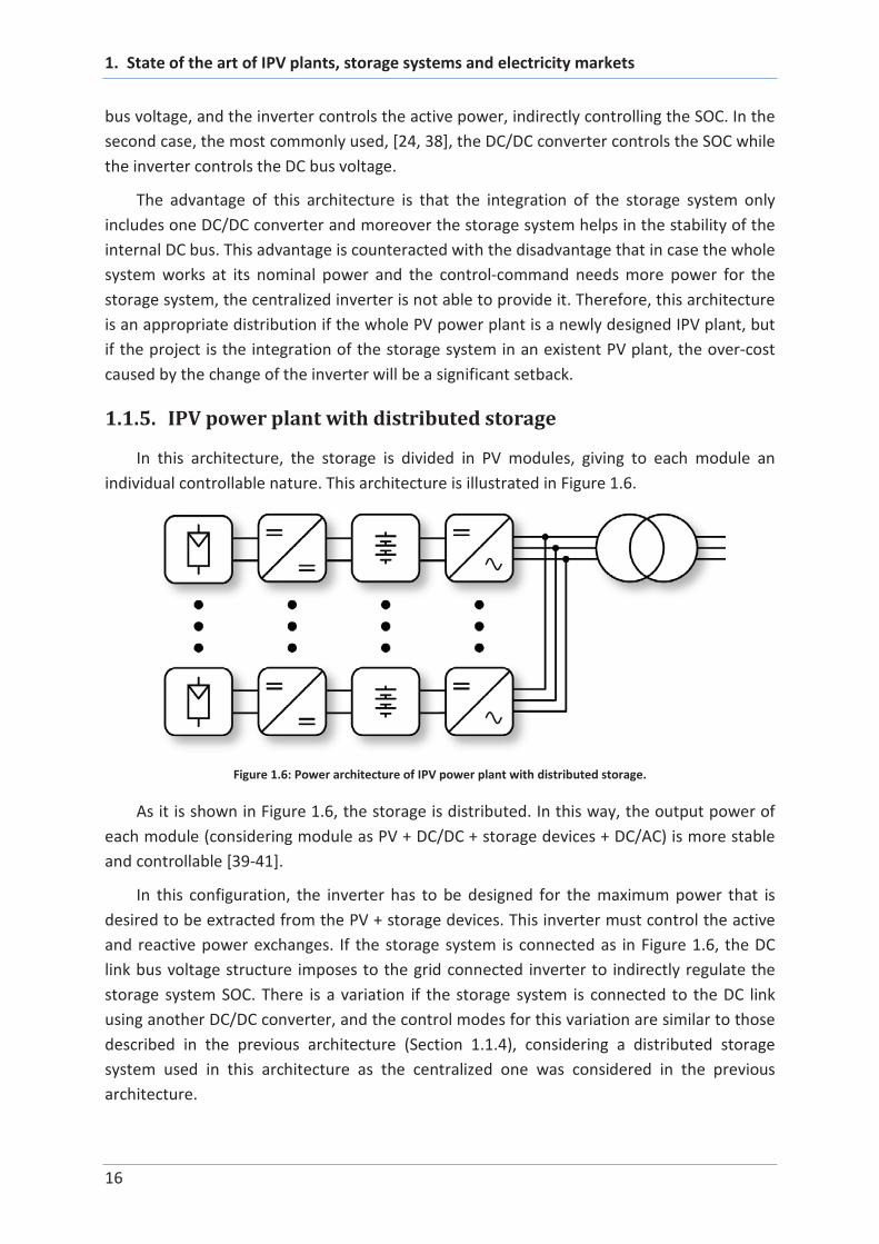
1.1.5. IPV power plant with distributed storage
In this architecture, the storage is divided in PV modules, giving to each module an
individual controllable nature. This architecture is illustrated in Figure 1.6.
Figure 1.6: Power architecture of IPV power plant with distributed storage.
As it is shown in Figure 1.6, the storage is distributed. In this way, the output power of
each module (considering module as PV + DC/DC + storage devices + DC/AC) is more stable
and controllable [39-41].
In this configuration, the inverter has to be designed for the maximum power that is
desired to be extracted from the PV + storage devices. This inverter must control the active
and reactive power exchanges. If the storage system is connected as in Figure 1.6, the DC
link bus voltage structure imposes to the grid connected inverter to indirectly regulate the
storage system SOC. There is a variation if the storage system is connected to the DC link
using another DC/DC converter, and the control modes for this variation are similar to those
described in the previous architecture (Section 1.1.4), considering a distributed storage
system used in this architecture as the centralized one was considered in the previous
architecture.
1. State of the art of IPV plants, storage systems and electricity markets
17
1.2. IPV plant control structure and management layers
After the power architecture description, in this section the control structure of the IPV
plant is presented. The control structure is another key factor for obtaining the wanted
reliability, stability and profitability of the IPV power plant.
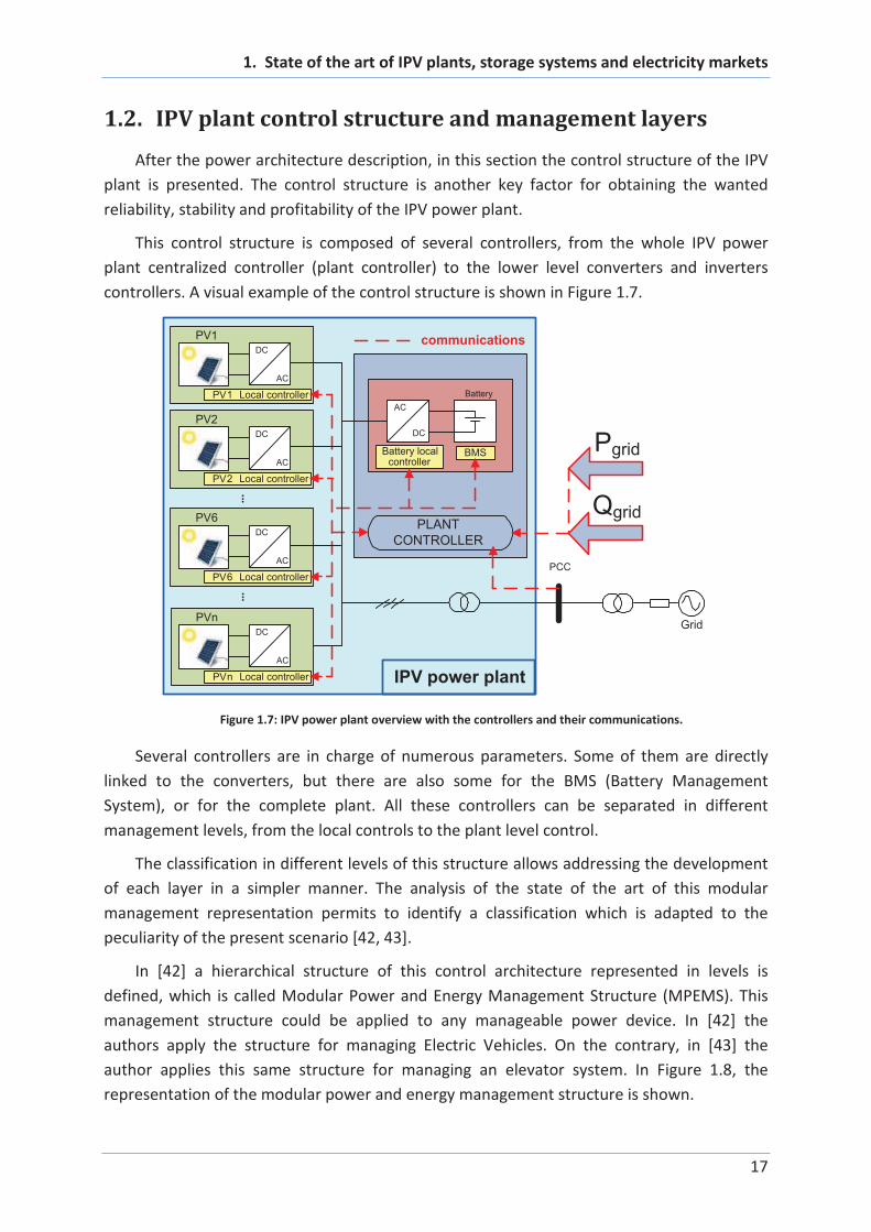
This control structure is composed of several controllers, from the whole IPV power
plant centralized controller (plant controller) to the lower level converters and inverters
controllers. A visual example of the control structure is shown in Figure 1.7.
Grid
PLANT
CONTROLLER
AC
DC
Battery localcontroller
BMS
PCC
Battery
communications
DC
AC
PV6
PV6 Local controller
DC
AC
PV2
PV2 Local controller
DC
AC
PV1
PV1 Local controller
...
IPV power plant
Pgrid
Qgrid
...
DC
AC
PVn
PVn Local controller
Figure 1.7: IPV power plant overview with the controllers and their communications.
Several controllers are in charge of numerous parameters. Some of them are directly
linked to the converters, but there are also some for the BMS (Battery Management
System), or for the complete plant. All these controllers can be separated in different
management levels, from the local controls to the plant level control.
The classification in different levels of this structure allows addressing the development
of each layer in a simpler manner. The analysis of the state of the art of this modular
management representation permits to identify a classification which is adapted to the
peculiarity of the present scenario [42, 43].
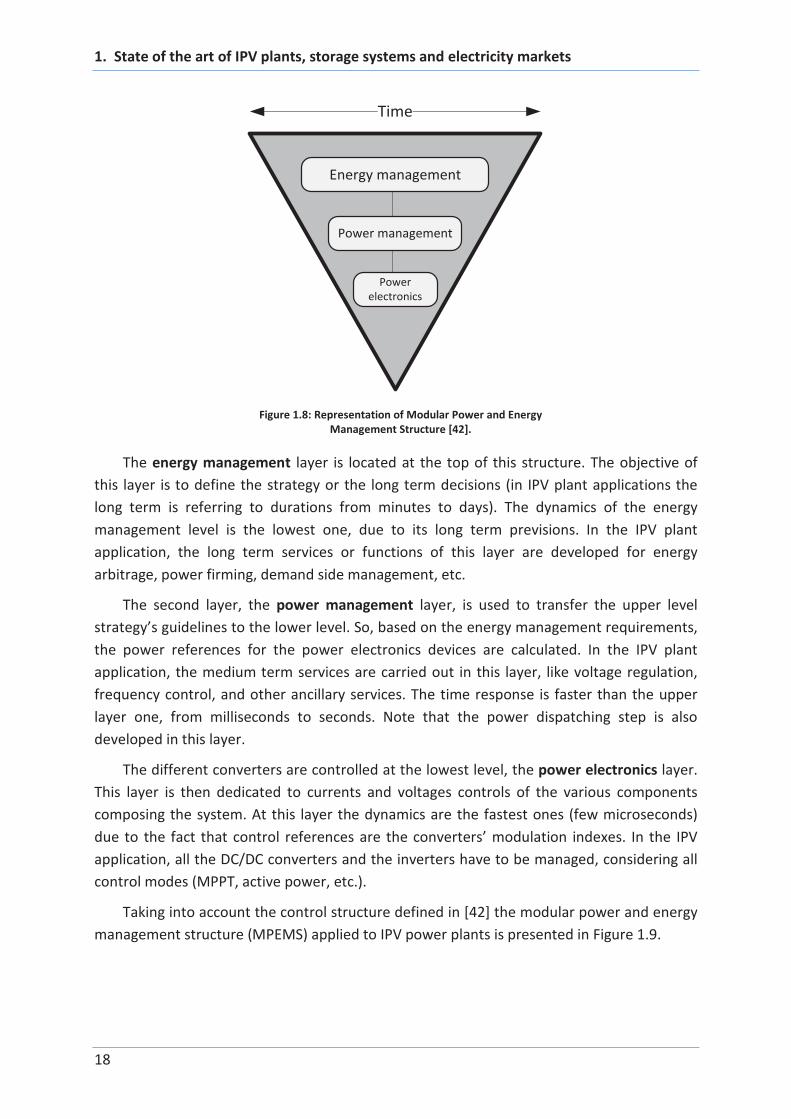
In [42] a hierarchical structure of this control architecture represented in levels is
defined, which is called Modular Power and Energy Management Structure (MPEMS). This
management structure could be applied to any manageable power device. In [42] the
authors apply the structure for managing Electric Vehicles. On the contrary, in [43] the
author applies this same structure for managing an elevator system. In Figure 1.8, the
representation of the modular power and energy management structure is shown.
1. State of the art of IPV plants, storage systems and electricity markets
18
Energy management
Power management
Power electronics
Time
Figure 1.8: Representation of Modular Power and Energy
Management Structure [42].
The energy management layer is located at the top of this structure. The objective of
this layer is to define the strategy or the long term decisions (in IPV plant applications the
long term is referring to durations from minutes to days). The dynamics of the energy
management level is the lowest one, due to its long term previsions. In the IPV plant
application, the long term services or functions of this layer are developed for energy
arbitrage, power firming, demand side management, etc.
The second layer, the power management layer, is used to transfer the upper level
strategy’s guidelines to the lower level. So, based on the energy management requirements,
the power references for the power electronics devices are calculated. In the IPV plant
application, the medium term services are carried out in this layer, like voltage regulation,
frequency control, and other ancillary services. The time response is faster than the upper
layer one, from milliseconds to seconds. Note that the power dispatching step is also
developed in this layer.
The different converters are controlled at the lowest level, the power electronics layer.
This layer is then dedicated to currents and voltages controls of the various components
composing the system. At this layer the dynamics are the fastest ones (few microseconds)
due to the fact that control references are the converters’ modulation indexes. In the IPV
application, all the DC/DC converters and the inverters have to be managed, considering all
control modes (MPPT, active power, etc.).
Taking into account the control structure defined in [42] the modular power and energy
management structure (MPEMS) applied to IPV power plants is presented in Figure 1.9.

1. State of the art of IPV plants, storage systems and electricity markets
19
Figure 1.9: Representation of the hierarchical control structure on the IPV application.
In Figure 1.9, a higher level control, which is not defined in [42], has been added. The
IPV power plant has an external link which is the market participation. The energy
management layer defines some market participation offers and the system operator (SO)
determines the amount of energy that has to be provided in each period of time. Therefore,
although the IPV power plant presents its market offers, it must accomplish the SO
requirements. This requirements are considered as the external control, which is managed
by the System Operator (SO) [44]. The SO dispatches the reference for the IPV power plant,
which are the inputs of the energy management control layer. By this communication line
between the SO and the IPV power plant, other grid services calls are made, as the
secondary regulation [45, 46], other ancillary services, etc. As the energy management
control receives the measures of the grid voltages and injected currents from its PCC, it
controls the active and reactive power exchanges depending on those measurements [47].
Focusing on the IPV’s scenarios, which are the core of the present work, the power
management can be a centralized control (as proposed in Figure 1.9) or a distributed one (at
the converters level).
The two highest control layers of the modular power and energy management
structure, which are the energy management layer and the power management layer, are
considered in the scope of the present work.
1. State of the art of IPV plants, storage systems and electricity markets
20
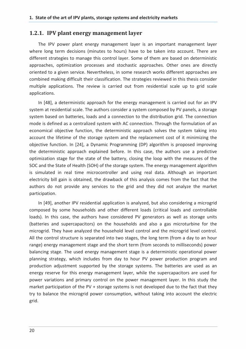
1.2.1. IPV plant energy management layer
The IPV power plant energy management layer is an important management layer
where long term decisions (minutes to hours) have to be taken into account. There are
different strategies to manage this control layer. Some of them are based on deterministic
approaches, optimization processes and stochastic approaches. Other ones are directly
oriented to a given service. Nevertheless, in some research works different approaches are
combined making difficult their classification. The strategies reviewed in this thesis consider
multiple applications. The review is carried out from residential scale up to grid scale
applications.
In [48], a deterministic approach for the energy management is carried out for an IPV
system at residential scale. The authors consider a system composed by PV panels, a storage
system based on batteries, loads and a connection to the distribution grid. The connection
mode is defined as a centralized system with AC connection. Through the formulation of an
economical objective function, the deterministic approach solves the system taking into
account the lifetime of the storage system and the replacement cost of it minimizing the
objective function. In [24], a Dynamic Programming (DP) algorithm is proposed improving
the deterministic approach explained before. In this case, the authors use a predictive
optimization stage for the state of the battery, closing the loop with the measures of the
SOC and the State of Health (SOH) of the storage system. The energy management algorithm
is simulated in real time microcontroller and using real data. Although an important
electricity bill gain is obtained, the drawback of this analysis comes from the fact that the
authors do not provide any services to the grid and they did not analyze the market
participation.
In [49], another IPV residential application is analyzed, but also considering a microgrid
composed by some households and other different loads (critical loads and controllable
loads). In this case, the authors have considered PV generators as well as storage units
(batteries and supercapacitors) on the households and also a gas microturbine for the
microgrid. They have analyzed the household level control and the microgrid level control.
All the control structure is separated into two stages, the long term (from a day to an hour
range) energy management stage and the short term (from seconds to milliseconds) power
balancing stage. The used energy management stage is a deterministic operational power
planning strategy, which includes from day to hour PV power production program and
production adjustment supported by the storage systems. The batteries are used as an
energy reserve for this energy management layer, while the supercapacitors are used for
power variations and primary control on the power management layer. In this study the
market participation of the PV + storage systems is not developed due to the fact that they
try to balance the microgrid power consumption, without taking into account the electric
grid.

1. State of the art of IPV plants, storage systems and electricity markets
21
Another residential IPV system is the Zero Energy Building (ZEB) developed by [18]. In
this work, the authors work with a grid-friendly hydrogen based ZEB, taking into account the
PV panels, a wind generator, house loads, the grid connection, an electric storage system
and a hydrogen storage tank with its electrolyzer and its fuel cell. The authors develop
optimized energy and power management strategies. The energy management layer is
composed by an adaptive optimization-based strategy called Adaptative Optimized Five-step
Charge Controller, which optimizes the overall operation cost and reduces the energy
exchange with the grid, turning on and off the electrolyzer and the fuel cell depending on
the battery SOC. The authors propose an optimization process applying the Genetic
Algorithm (GA) to determine the most well suited fuel cell and electrolyzer turning on and
off thresholds, but it is not considered to provide any direct services to the grid. The
limitation of the study comes from the fact that the market participation is not evaluated,
while the grid connected and the stand-alone modes are analyzed.
At grid scale, in wind power application, there are also installations of energy storage
systems and in this case they could be named Intelligent Wind Power or IWP. Several
research works are also focusing on this type of systems, related to the energy management
subject. In [50], the authors consider a wind/hydrogen/supercapacitor hybrid power system.
The objective of the control system is to make controllable the generated wind power to
provide some ancillary services to the grid (voltage and frequency regulation). The authors
also separate three control layers as the above mentioned MPEMS, but with different layers’
names. In MPEMS’ energy management layer, the authors develop two control strategies,
which are called “grid-following” and “source-following”. The control strategies, as their
names mention, regulate the power related to the grid and to the source. The authors
conclude that the one that regulates the power related to the source, the “source-following”
control strategy, is better because counteracting the source fluctuations by the energy
storage systems, the complete system output power has better performances on the grid
regulation. The limitation of the present study is mainly the lack of grid services, despite the
development of control strategies.
The papers [51, 52] are also dealing with the IWP application, but in this case, they use a
sodium sulphur battery as energy storage system (ESS) connected to a wind power farm. For
decreasing the day-ahead forecast errors of the stochastic behavior of the wind power
production, the authors use an autoregressive model. For analyzing the behavior and the
performance of the ESS, they use a Monte Carlo simulation tool. The authors use the ESS to
mitigate the forecast errors in order to fulfill the day-ahead power production commitment
and they assess the storage performance using a Mean Absolute Deviation criterion. It is a
relevant study which considers the day-ahead commitment (which could be developed by
electricity markets), but did not take into account the SOC and ageing level for determining
this day-ahead commitment.
Finally, considering the grid scale IPV power plants, in [53], the integration of an energy
storage system into a PV power plant is analyzed. In this work, the energy management layer

1. State of the art of IPV plants, storage systems and electricity markets
22
is considered one important fact, and thus it is widely developed. Two main energy
management strategies are described which are the constant power steps control strategy
and the fluctuations reduction control strategy. Within those energy management
strategies, the author has developed multiple complementary control options that are
introduced into the power management layer. In the energy management constant power
steps control strategy, the author has differentiated between one single constant step,
multiple constant steps, and hourly-adapted constant steps per day. This energy
management strategy is perfectly adapted to the electricity market pool participation. In this
strategy, the ESS has to inject or absorb the difference between the committed step values
and the PV production. The other energy management strategy is the fluctuations’ reduction
control strategy, also called smoothing control strategy. This one uses the ESS capacity as a
real energy buffer or as energy filter, filtering the fluctuations of the power variation caused
by the instantaneous solar irradiation variations, also called clouds effect. Depending on the
filter’s time constant the variations will be more flattened or not, and in conclusion, with a
greater filter’s time constant, the ESS energy capacity has to be higher. This energy
management is better adapted for cloudy days, in order to not introduce disturbances into
the electric network, but it cannot be used to introduce the IPV power plant in the electricity
market.
The constant power steps control strategy, as it is perfectly adapted to electricity
market participation, is the base study for the development of the present PhD study, where
the hourly steps will be optimized, maximizing the economic exploitation of the IPV power
plant based on an innovative market participation. This development is discussed in detail in
chapter 2.
1.2.2. IPV plant power management layer
Getting back to the MPEMS and having explained the upper layer, i.e. the energy
management layer, in this section, the focus is made on the power management layer. All
power management layer strategies are oriented to given services as balance control, ramp
rate control, frequency control, peak shaving, inertia response, back up service, islanding
mode, fluctuation reduction control, voltage control, etcetera. The applications that are
going to be analyzed are the wind energy and the PV systems because the wind energy has
similar disadvantages from the grid point of view compared to the application of the present
work, the IPV power plants.
As mentioned before, for the energy management layer, the use of an ESS is almost
necessary, but for the power management layer, it is not totally required. For that reason,
the first application here described includes a power management layer without ESS, but
providing some ancillary services to the grid by a wind farm. In [54] the power design of the
wind farm controller is explained, providing better grid integration characteristics. The
implemented control functions are: balance control, delta control, power ramp rate
limitation, automatic frequency control, reactive power control and automatic voltage

1. State of the art of IPV plants, storage systems and electricity markets
23
control. As it will be shown afterwards, these functions can be provided by the ESS, but in
this case, they are provided by the wind farm, by means of reducing its power production.
For that reason, the use of an ESS may be a better solution for providing those functions
(through its charge and discharge) instead of decreasing the power production point, thus
reducing the wind farm generation from the optimal production point.
In [55], a wind farm is also assessed but in this case the application is an IWP system: a
wind farm with storage capacity. The relevance of this work lies in the fact that the proposed
controls are tested in a real facility composed by 12 MW of wind power and 1.6 MW of
lithium-ion battery energy storage system. Tested controls are the primary reserve, or the
frequency support, the inertia response and the power oscillation damping. On this power
management layer, once the mentioned controls are operated, the power dispatch is carried
out, for distributing the power references between the wind generators and the energy
storage system.
Another IWP application analysis is carried out in [50]. As explained in the previous part,
the authors consider a wind/hydrogen/supercapacitor hybrid power system and separate
the energy management layer and the power management layer. The power management
layer is called Automatic Control Unit (ACU). In this unit, they have separated the power
management control for each power device, which are the wind generators, the
supercapacitor, the electrolyzer, the fuel cell and the grid connection unit. The control
strategy is applied using PI controllers in order to regulate the desired variable of each unit
and without causing controlling conflicts between controllers.
The power management layer is also analyzed in [49]. The IPV residential application
that has been worked with considers PV generators, batteries and supercapacitors. The
authors consider an IPV residential application but they also consider a microgrid composed
by some households and other different loads (critical loads and controllable loads). In the
power management layer of the IPV household, the authors have presented a strategy to
manage solar energy resources and grid requirements, having a primary frequency control
mode as well as a PV limitation mode, a storage mode but no real time power dispatching
mode. Depending on the working mode, the PV, the batteries and the supercapacitors are
controlled on a different control method.
Hydrogen based grid-friendly Zero Energy Building (ZEB) developed by [18] proposes
another residential IPV system. Authors develop optimized energy and power management
strategies. The power management layer includes some auxiliary services (peak-shaving and
Reactive Power Control (RPC)) and a back-up service. In the ZEB facility the auxiliary services
together with the back-up service are implemented in the electric energy storage control
and fuel cell and electrolyzer operation is commanded taking into account the energy
management references. This power management layer is simulated in a RT-Lab real-time
simulation platform, where the interaction between the energy management layer and
power management layer are tested.

1. State of the art of IPV plants, storage systems and electricity markets
24
In [56], another IPV system is presented composed by a PV - lithium-ion battery -
supercapacitor system. In this case, the IPV system supplies the needed energy of a
microgrid. Nevertheless, this microgrid is also connected to the main grid. The power
management presented in this work explains a state machine control strategy, taking into
account the following states: black-start, islanding and grid-connected. The power
management strategy describes a control structure enabling, through the supercapacitor
system, fast variations (low energy and high power value) and enabling also, through the
lithium-ion battery system, the possibility to balance the PV production and the
consumption of the loads (high energy and lower power value).
For the above mentioned energy management strategies, the author in [53] has
developed multiple power management complementary controls which are: 1) preferred
state-of-charge, 2) power change rate limitation, 3) meteorologically-based adjustments, 4)
steps optimization, and 5) predictive control for constant steps value. In the scope of this
work, the most important control is the predictive control for constant steps value. This
control is also developed in [27]. In this control, the future prices of the electricity and the
SOC of the ESS are considered in order to decide whether the commitments are going to be
accomplished or not, accepting the corresponding penalties.
The Wakkanai Mega Solar Park, in Japan, is composed of 5MW of PV panels and 1.5 MW
- 11.8 MWh of Sodium Sulphur (NaS) battery system [15, 16, 57]. In the power management
layer, the NaS battery system is used to reduce the short term fluctuations of the PV
production through different strategies: a Moving Average (MA) method and a HYbrid (HY)
method. The HY method selectively uses the MA and the Fluctuation Center Following (FCF)
methods according to the fluctuation magnitude. In [57], a comparison of these two
methods is carried out.
The last project analyzed in this state of the art is the European Union supported ILIS
project, Innovative Lithium-Ion System management design for MW solar plants [13]. This
project integrates a 1 MW - 560 kWh lithium-ion battery energy storage system to a 1.2 MW
PV power plant in Navarre, Spain (Figure 1.10). In [14], the developed power management
layer proposes some ancillary services (constant power production, active power ramp rate
limitation, frequency control function and voltage control function). The imperative need of
a centralized plant controller is demonstrated for the improvement of the PV systems
integration into the grid. This power management layer calculates the ancillary services
responds (power references) and dispatches them around the lower level, which is the
power electronics layer. The advantage of the use of the ESS is clearly concluded with the
different control modes, showing the results obtained with and without the use of the ESS.

1. State of the art of IPV plants, storage systems and electricity markets
25
Figure 1.10: Aerial picture of the ILIS project PV power plant demonstrator.
1.3. Energy storage systems
Energy storage systems are one of the key elements to solve the biggest electric grid
challenge: the imperative constant balance between production and consumption.
Moreover, it is also important for a lot of different applications which are not always
connected to the electric grid. In these applications the storage system provides the energy
needed to autonomously work during a specific period of time. And, in the present issue, it is
also a key element for a well-suited integration of the RESs to the electric network, due to
the fact that it allows the flexibility, reliability, availability and efficiency of these variable
and unpredictable energy sources [13-18, 53, 58, 59].
1.3.1. Energy storage systems’ technologies
The energy storage system could be classified depending on their technology or their
work principle, as mechanical, electromagnetic, electrochemical and thermal [60]. As
summarized in [53, 61, 62], a detailed classification of energy storage technologies is shown
in Figure 1.11.
Depicted electromagnetic storage technologies are ultracapacitors or supercapacitors
and Superconducting Magnetic Energy Storage (SMES). Mechanical storage technologies are
Pumped Hydroelectric Storage (PHS), Compressed Air Energy Storage (CAES) and Flywheel
Energy Storage (FES). Electrochemical technologies are separated into Battery Energy
Storage (BES), Flow Battery Energy Storage (FBES), air batteries and hydrogen based storage.
BES can be differentiated into lead acid batteries, nickel cadmium (NiCd) or nickel metal
hydride (NiMH) batteries, sodium sulphur (NaS) batteries, zebra batteries and lithium-ion (Li-
ion) batteries. FBES, could also be divided into vanadium redox batteries and zinc bromine

1. State of the art of IPV plants, storage systems and electricity markets
26
batteries. Finally, thermal operation principle energy storage is formed by the High
Temperature Thermoelectric Energy Storage (HT-TES) and Low Temperature Thermoelectric
Energy Storage (LT-TES).
Energy storage technologies
Electromagnetic
SMESSupercapacitors
Mechanical
PHS CAES FES
Electrochemical
BES FBESAir
batteriesHydrogen
Thermal
HT-TES
Vanadium redox
Zinc bromine
Li-ionNaS Zebra
LT-TES
Lead acidNiCdNiMH
Figure 1.11: Classification of energy storage technologies [53, 61].
Some of these technologies are more suited for the integration of RESs [50, 56, 63-65]
due to their characteristics. Note that some of them, like PHS or CAES, require some natural
conditions to operate. Nowadays the most emerging technologies are the electrochemical
ones and mainly the battery based energy storage systems. Among them, even if lead-acid
and nickel based technologies have solid market share due to their maturity and low cost,
sodium sulphur and lithium ion are the most installed technologies. Lithium based
technologies are expected to dominate the market in a mid-term perspective. An example of
this fact is shown in [59], where it is stated that actually one third of all ESS projects are
based on lithium-ion technology.
The characteristic parameters to determine the appropriate technology for each
application are explained in the following sub-section.
1.3.2. Energy storage systems characteristic parameters
As it has been explained before, there are several technologies of storage system and
each one of them has its main characteristics. For each application, some characteristics are
much more important than others. In this case, for the integration of RESs, the identified
most representative technical parameters of an energy storage system are the next ones
[53, 66-68]:
Power capacity [W]: It is the maximum power that the ESS could provide. Its charge
power capacity and its discharge power capacity can be different.
Energy capacity [Wh]: It is the amount of energy that the ESS could store. It is also
named as capacity (C) and measured in Ampere-hours [Ah].
Power to energy ratio [W/Wh]: It describes the ratio between power and energy.
C-rate: It specifies the speed of charge or discharge rate of the storage system. It
determines the storage system’s charge or discharge current in relation to its
nominal capacity which is expressed by the letter C and measured in Ampere-hours

1. State of the art of IPV plants, storage systems and electricity markets
27
[Ah]. A charge or discharge of nC rate means that the capacity of the storage system
will be charged or discharged in 1/n hours. For example, a 50 Ah storage system
which is being discharged at 2C rate implies a 100 A current and a 0.5 h discharge
time.
Energy density [kWh/m3]: It represents the available energy per volume unit.
Specific energy [kWh/kg]: It quantifies the ratio of the energy delivered to its weight.
Power density [kW/m3]: It defines the available power per volume unit.
Specific power [kW/kg]: It depicts the ratio of the power delivered to its weight.
Energetic efficiency [%]: It shows the relation between the discharged energy and
the amount of energy needed to restore the initial charge state, under specific
conditions. It is measured in percentage.
Life cycles [cycles]: It determines the quantity of consecutive charge and discharge
processes that a battery can undergo while maintaining some minimum
performances.
Calendar life [time]: It determines the period of time in which the battery maintains
some minimum performances without being used.
The Electricity Storage Association [60] shows some figures of several storage
technologies which include two parameters’ relation. In Figure 1.12, the relation between
the discharge time and the rated power is depicted, where it can be concluded that for large
scale energy storage systems the PHS is the most appropriated technology. In this figure,
knowing the discharge time and the rated power, the energy capacity parameter can be
obtained, and for that reason, this figure is one of the most illustrative ones to evaluate the
power and energy rates of each technology.
Figure 1.12: Energy storage technologies discharge time versus their rated power [60].

1. State of the art of IPV plants, storage systems and electricity markets
28
From Figure 1.12 it can be observed that the characteristics of the lithium-ion
technology are wide and cover a large region, from large discharge time (over 10 hours) to
rated power that overpasses the MW range. Other technologies as lead acid or sodium
sulphur have a larger rated power characteristic compared to the lithium-ion technology.
In Figure 1.13, two other important parameters are shown, which are the technology
efficiency and the lifetime. These two parameters are proportionally related to the energy
storage system cost. On the one hand, the efficiency means losses of energy while charging
and discharging the storage system. On the other hand, if the purpose is to cycle the ESS
thousand times, the replacement cost has to be evaluated. Thus, this figure is also very
illustrative to evaluate the technologies’ performances.
Figure 1.13: Energy storage technologies’ efficiency versus their lifetime [60].
The most beneficial area of this Figure 1.13 is the upper right side of the figure, for being
very efficient and for having a long lifetime. As it can be extracted, the lithium-ion
technology has very high efficiency with a lifetime of several thousands of cycles, so it is
demonstrated that currently it is a relevant technology. The characteristics of the other
electrochemical technologies are not so good as the ones of the lithium-ion technology.
1.3.3. Energy storage system sizing methods
As stated in the introduction of this document, the sizing process of an energy storage
system is one of the key factors of the present work. The sizing process which includes the
definition of power and energy requirements is totally correlated with the management of
the storage system, and for that reason, the sizing process has to be co-performed with the
energy management strategy.

1. State of the art of IPV plants, storage systems and electricity markets
29
An example of this significant correlation is explained in [23] and shown in Figure 1.14.
The power requirement for an energy storage system is the instantaneous value between
the PV power production curve (the black one) and the other curves (the power
commitment with different energy management strategies, EMSs). As it is shown, the hourly
constant power step curve (the orange one, named HCPS) represents the configuration
requesting a lower power, because it is continuously close to the PV power production
curve. The energy requirements’ value is the area drawn between the PV power production
and the commitment curves. In this case, the single constant power step curve (the red one,
named 1SCPS), which was established by a simpler EMS, needs the highest energy value.
Figure 1.14: Real PV power production pattern and different power
commitment according to different EMS configurations [23].
Together with this figure, in the same study, the energy storage sizing is conducted
taking into consideration also a simulation of a whole year and still applying each of these
three EMS. The results of these simulations are shown in Table 1.1, where the percentage of
time that the IPV power plant cannot track the EMS calculated grid power is presented as a
function of the storage system capacity. This percentage of time that the IPV power plant
cannot track the EMS calculated grid power is due to the fact that the storage system is
saturated, upward (fully charged) or downward (fully discharged). As it can be seen, with a
simpler EMS configuration as the SCPS, the storage system is saturated much quicker than
with more complex strategies. The HCPS, which is the most complicated one, has then the
best results with regards to the other storage systems sizing.
Table 1.1: Percentage of time that the IPV power plant cannot track the EMS calculated grid power as a function of
the storage system capacity. Source: [23].
EMS
configuration
Capacity
0.2 pu
Capacity
0.25 pu
Capacity
0.3 pu
Capacity
0.35 pu
Capacity
0.4 pu
Capacity
0.45 pu
Capacity
0.5 pu
SCPS 9.32 5.40 2.94 1.79 1.08 0.61 0.29
4LCPS 2.68 1.48 0.88 0.50 0.29 0.18 0.11
HCPS 1.63 0.94 0.64 0.37 0.26 0.16 0.09

1. State of the art of IPV plants, storage systems and electricity markets
30
As a conclusion, with a more complex energy management strategy, lower power and
energy requirements are needed and vice versa. For matching these two criteria several
sizing methodologies have been described in the literature.
In [69] and in [43] one sizing methodology is presented, which will be the base for other
methods explanation. This methodology is separated into three steps, which are the
definition of system requirements, the sizing of the energy storage system and the
verification of possible solutions. In Figure 1.15, graphical illustration of this methodology is
proposed.
Figure 1.15: Energy storage system sizing methodology [43].
In this first step, the definition of the system requirements is done as well as the system
constraints’ definition. The storage system’s requirements are the power and energy needs.
Other important requirements are the energy and power management strategies. In order
to determine the optimal sizing of the energy storage system, the energy management
strategy definition is necessary. The energy storage system constraints are related to the
characteristics of the application. In this case, these are: the connection voltage to the grid,
the volume and the weight of the storage system, the operation temperature and the
efficiency. But there are some other constraints that are not related to the application, like
lifecycles, calendar life, capital and BMS cost and maintenance cost of the storage system.
In the second step, the energy storage sizing is calculated, taking into account the
system requirements and constraints. In order to achieve the system’s requirements, several
solutions can be considered. The third step consists thus in verifying the possibilities and
evaluating the options before going back to the first step for changing some requirements or
constraints in order to improve the final sizing result. In this feedback, the energy and power
management strategy could be changed to calculate the optimal sizing for that new strategy.
With several strategies/sizing relation results, the optimal storage sizing could be selected
considering its optimal strategy.
The energy management strategy is introduced in the first step, as one of the definitions
of the system requirements for the following sizing process. It has been decided to select
first the energy management strategy in order to size the storage system based on this
strategy. Nevertheless, the energy storage sizing methods can be separated by their nature

1. State of the art of IPV plants, storage systems and electricity markets
31
and they can also be grouped in different categories. As a first work, a classification based on
the nature of each sizing method is proposed and shown in Figure 1.16.
Energy storage sizing methods
Stochastic
Monte Carlo Probabilistic
Deterministic
Rule based Extrema
Service oriented
Load following
Peak shaving
Figure 1.16: Proposed energy storage sizing methods classification by their nature.
1.3.3.1. Stochastic energy storage sizing methods
Stochastic methods for energy storage sizing are, as their name indicates, methods that
are dependent to predicted values and also dependent to some random elements. The
probability methods are, thus, included in this group.
Monte Carlo method
Monte Carlo sizing method is a stochastic method. It randomly generates some inputs
(in this case sizing parameters) and verifies if those inputs accomplish the required
performances. The more iteration, the better result is.
For energy storage sizing, this method is used in [70], where an IPV application at the
residential scale is considered. Taking into account load profiles, weather forecasts and the
local historical outage distribution of a household, the Monte Carlo method calculates
energy storage sizing parameters for the demand shift at peak electricity cost and outage
protection objectives.
Another energy storage system for wind power application is analyzed in [51]. The
authors use an autoregressive model to obtain the correlation of the day-ahead forecast
errors. Afterwards, they quantify the impact of this correlation with the storage sizing by
means of a Monte Carlo approach, using the autoregressive model as input. Taking into
account the time when the storage system is saturated (totally charged or discharged), the
authors are able to compute an optimized size of the storage system.
Probabilistic approach
A probabilistic approach is another stochastic method based on probability. Its first step
or its input is the predicted value(s). From this data, the probability of having an error is
calculated and error probability areas are obtained as shown in Figure 1.17.

1. State of the art of IPV plants, storage systems and electricity markets
32
Figure 1.17: Probability of wind power generation forecast error [71].
The sizing problem also appears for wind energy applications with an energy storage
system. In [71] the sizing problem tries to minimize the power production forecasts errors,
assuming the market conditions where penalties are considered. Based on a probabilistic
forecast, the sizing requirements could be minimized.
In [72], another IWP application where the storage sizing is carried out through a
probabilistic approach is developed. The objective of the proposed method is the reduction
of the uncertainty on wind power forecasts (up to 48 hours), analyzing the statistical
behavior of the forecast error as well as the SOC. Empirical probability density functions are
developed reducing the size of the ESS and the uncertainty of the IWP system.
1.3.3.2. Deterministic energy storage sizing methods
Deterministic methods for energy storage sizing are, as their name suggests, methods
that are not dependent to randomness to calculate inputs/outputs’ relationship.
Rule based method
Rule based method is a simple method that contains some rules. It applies the desired
control output to the given inputs of the system. It is an applied method that can be used as
a benchmark to assess other more advanced techniques.
For an IPV grid scale application, in [23], the sizing process relation with the energy
management system is analyzed and discussed. The authors have developed three EMSs
that are 1) one single constant power step; 2) four-level constant power step; and 3) hourly
constant power step (HCPS). These energy management strategies are based on rules, so
they could be considered as rule based methods. For each of these EMSs and for a different
capacity sizes, the authors have calculated the percentage of the time the IPV power plant
cannot track the reference grid power. These different sizing capacities are selected
depending on the PV plant capacity factor, which is the equivalent value of energy that each
kW installed could produce per day. Thus, the sizing is not calculated but analyzed related

1. State of the art of IPV plants, storage systems and electricity markets
33
with the EMS configurations. Nevertheless, they have showed that with the HCPS strategy,
the energy requirements are much lower than in the other energy management strategies.
Extrema method
Extrema method is a deterministic strategy which makes a grid search of a set of input
values and obtains their feasibility range to keep the optimal solution.
In [73], the application of an industrial customer with a battery energy storage system is
considered. The objective service is the peak load shaving, but the methodology used for the
calculus of the sizing is optimized maximizing the customer’s economic benefits. For doing
so, the sizing and the operating steps are developed using the “extrema” method for
optimizing the sizing problem and using dynamic programming strategy for the operation
optimization. Dynamic programming is an optimization method for large decision problems
which breaks the problem into smaller sub-problems, separately solving each one of them
and obtaining an optimal decision policy [74].
1.3.3.3. Service oriented energy storage sizing strategies
The strategies included in this section are completely oriented to provide a given
service. Multiple applications could be taken into account but only the ones related to grid
services are considered in this section.
Load following strategy
The objective of this strategy is to adjust the output power to the demand of electricity.
When the demand is important, this strategy leads to produce more, and when the demand
is low, the strategy decreases the generation. In the case of an energy storage system, it
could refer to absorb energy.
In [75], the analyzed application is a residential distribution feeder where a battery
energy storage system is installed. The objective (the service to be provided) is the shaving
of the peak where a percentage of the peak power is selected setting a lower peak value.
From this value the power requirement is calculated, and with an analysis of the time when
this value is exceeded, the energy requirement is also obtained. This method is referred as
load following method. In this paper, the impact of the distributed PV generation in a BESS
sizing is briefly analyzed, concluding that the power sizing is maintained and the needed
amount of energy (for the storage) is reduced.
Peak shaving strategy
The objective of this strategy is to reduce the peak power providing an amount of
energy from the storage system, reducing the given peak. This service is used to avoid a
higher power contract in end user applications (residential and commercial) and also to
avoid having to repower a substation, from the grid operator point of view.

1. State of the art of IPV plants, storage systems and electricity markets
34
A residential application equipped by a BES/PV system is analyzed in [36, 76, 77]. The
authors have studied the sizing problem, proposing upper and lower bounds for the storage
size and two algorithms to calculate the exact storage size taking into account a fixed load
curve and time-of-use electricity purchase rate. The provided services are power arbitrage
and peak shaving and the objective is to minimize the purchase cost from the grid with the
optimal battery size while satisfying the fixed loads. It has been verified that for certain
scenarios, the characterization of the exact storage size is achievable, but without
considering the loads variation possibility as well as real hourly changes in electricity
purchase.
1.4. Electricity market analysis
In this section, an electricity market analysis is proposed. This state of the art review
concludes with an analysis of the market where the IPV power plants could seek for an
economical viability through their participation. The electricity market selected is the
Spanish one, due to the fact that Spain is one of the European countries with higher
renewable energy integration level.
Similarly to the other European electricity markets, the liberalization of the Spanish
sector was established in the 90s [78]. Since that moment, the sector regulation laws have
been gradually signed as well as renewable sources referred laws [79-82]. In the first laws,
important incentives, financial support and feed-in-tariff were signed [81, 82], which heavily
increased the Spanish photovoltaic share. Nevertheless, by means of other laws, these
incentives decreased after that [80], until recently (2013) [83, 84]. These last laws have
dramatically stopped the renewable energies’ incentives.
In this context, the situation for the renewable generation systems over the coming
years is that they could participate on the electricity markets in the same conditions, with
the same rights, the same obligations and without any incentives as other traditional
generation units. So the next section describes the organization of the electricity markets
and the markets where the IPV power plants could potentially participate.
1.4.1. Organization of electricity markets
Throughout all Europe, most electricity markets are similar and have the same markets:
futures markets, daily market (day-ahead market), intraday markets and operation markets
(system adjustment markets). The organization of the electricity markets is distributed in the
previously mentioned markets where requirements for offering and bidding are different
among all of them. Each market is organized in a different way and the Iberian Peninsula
case is summarized in the Figure 1.18.

1. State of the art of IPV plants, storage systems and electricity markets
35
Figure 1.18: Iberian organization of the electricity markets.
“Not organized” markets are energy contracts between some producers and some big
consumers like an industrial factory.
The Iberian electricity market (MIBEL, Mercado Ibérico de la Electricidad) [85] is the
market where almost all of the energy needs are negotiated, using different markets. In the
future markets, which are managed by the Portuguese section of the Iberian Market
Operator (OMIP, Operador del Mercado Ibérico – Polo Portugués), long term contracts
(week, month, quarter and annual) are auctioned [86]. The other MIBEL’s markets, the daily
and the intraday markets, are managed by the Spanish section of the Iberian Market
Operator (OMIE, Operador del Mercado Ibérico – Polo Español) [87].
Daily market, also known as pool market, is important because its objective is to match
the whole energy that will be consumed on the following day [88, 89]. The Market Operator
(MO) receives the producer and consumer’s offers for each programming period (an hour
period in that case). With those offers the matching process is carried out starting from the
lowest offers until the crossing point between the offer and the demand with the lowest
price in each programming period. That price is known as marginal price. Generators and
consumers that have presented a lower generation offer (and greater consumption offer)
than the marginal price are scheduled for generation/consumption (power commitment)
and are paid at the marginal price.
Besides the daily market, which has been resolved on the previous day, another market
exists which is the intraday market and it is resolved closer to operation time. It is not always
possible to match the forecasted consumption profile with the daily market scheduled
power, and these differences are solved by the intraday markets. In the Iberian markets’
case, six intraday markets exist, where the same process as in the daily market is carried out
despite the fact that each intraday market has a different duration [89], from 27 hours to 9
hours.
An example for the daily market matching process for the hour 12 of the 7th August
2015 is presented in Figure 1.19.
OMIP
OMIEPRODUCER
SELLER
CONSUMER
BUYER
SO... ...

1. State of the art of IPV plants, storage systems and electricity markets
36
Figure 1.19: Daily market matching process curves of generation and consumption of the hour 12
(from 11:00 to 12:00) of the date 2015/07/08 [87].
Once the daily market has been closed by the OMIE, the information is transferred to
the System Operator (SO), REE (Red Eléctrica de España) (P.O. 9.0) [90], which makes the
necessary technical adjustment and restrictions (P.O. 3.2 and P.O. 3.10) [91, 92]. After this
adjustment, the final matching curves are generated, also visible in Figure 1.19, where the
final marginal price for each hour is defined. The System Operator also organizes the
deviation market, (P.O. 3.3) [93], if necessary, and the ancillary services market. As ancillary
services, the Iberian System Operator, REE, considers the voltage control (P.O. 7.4) [94], an
additional reserve power to be raised (P.O. 3.9) [95] and frequency regulation. Regarding the
frequency regulation service, the primary (P.O. 7.1) [96], secondary (P.O. 7.2) [97] and
tertiary (P.O. 7.3) [98] reserves are taken into account. In the Iberian electricity system the
primary regulation is a compulsory service that all generators must provide and it is not
remunerated.
The last market or power exchange identified in Figure 1.18 is carried out at an
international level (P.O. 4.0) [99], including daily markets as well as two intraday markets
with France (P.O. 4.1) [100], and daily markets with Morocco and Andorra. These markets
are bidirectional, but the power exchange is not always transferred from both countries.
1.4.2. Operation of traditional generators on electricity markets
In this section, the operation of traditional generators on electricity markets is detailed,
explaining the process of the most important markets and the timing when offers must be
sent to the market operator. A general overview of the mentioned markets is shown in
Figure 1.20.

1. State of the art of IPV plants, storage systems and electricity markets
37
Figure 1.20: Iberian Peninsula electricity markets operation schedule and offers sending period of time.
1.4.2.1. Daily market
The daily market is the most important market of electricity because the whole part of
daily energy transactions are bidden and cleared in this market. It is also known as electricity
pool market. The horizon of this market is composed by the 24 hours of each day.
Generators prepare their generation planning and try to clear themselves in this market.
The planning offers (for the daily market) to the day D must be sent to the market
operator before midday of day D-1, as shown in Figure 1.20 [10-12]. These offers (or bids)
are composed by an amount of energy at a given price for each market period, normally an
hour.
The market operator clears each market period and sends the results to the system
operator. The system operator includes the technical constraints concluding with the viable
daily schedule [11]. This schedule is sent to all generators, including the cleared amount of
energy to produce and the associated marginal price for time step (each hour).
From this moment on, if the offers sent by a generator are accepted, they must be
provided as cleared energy, during the cleared market periods of the day D. If the offers are
not accepted, the concerned generators do not have to produce energy in this period of
time. This means that all generators willing to participate in the daily market need to have
very reliable production predictions on a day-ahead basis, to be able to make feasible offers.
As the generation plan is based on the day ahead predictions of generation and
consumption, errors are to be expected on these predictions. Moreover, as the daily market
cleared energy is resolved by means of offer and demand laws, not all the electricity needs
are solved. For that reason, the market participation is not only based on the daily market,
and the differences in consumption needs are solved taking advantage of the intraday

1. State of the art of IPV plants, storage systems and electricity markets
38
markets, which are closer to the real time operation. The closer the market period is to real
time, the better the system operator consumption predictions are.
1.4.2.2. Intraday market
Intraday markets exist to clear the consumption needs that have not been resolved
through the daily market. It can be considered as some kind of adjustment markets. All
generators that have participated in the daily market can participate in the different sessions
of the intraday market [11]. In the Iberian Peninsula the six intraday sessions are operating
on different time horizons, which are depicted on Figure 1.20 and detailed in Table 1.2 [11].
Table 1.2: Intraday sessions detailed information.
Intraday sessions
S1 S2 S3 S4 S5 S6
Session opening 17:00 21:00 01:00 04:00 08:00 12:00
Session closing 18:45 21:45 01:45 04:45 08:45 12:45
Program publication 20:45 23:45 03:45 06:45 10:45 14:45
Schedule horizon 27h 24h 20h 17h 13h 9h
Operation starting 21:00 00:00 04:00 07:00 11:00 15:00
Market participators (also named market agents) can offer a purchase or sale bids. So,
the generators can sell and buy energy, adjusting their operation program. The market
operator clears each market period and sends to the system operator the cleared powers
and prices. The system operator publishes then the final program, including the technical
constraints. This program is named the hourly final program (PHF, in Spanish) [11].
As it could be verified in Table 1.2, the period between the session closing and the
operation starting time is closer than in the daily market, which offers the availability to
present more performing bids from all generators, and especially from renewable
generators, based on closer and better predictions. Another important remark that can be
done about the intraday market is that there is a market session every 3-4 hours (except
between session 6 and session 1 of the next day, where there are 6 hours). This fact provides
the opportunity to adjust all generation programs each 3-4 hours.
1.4.2.3. Ancillary services
The Iberian System Operator, REE, considers as ancillary services voltage control,
additional reserve power to raise and frequency and power regulation (with primary,
secondary and tertiary reserves). The primary regulation or frequency regulation (P.O. 7.1)
[96] is a compulsory service that all generators must provide and it is not remunerated.

1. State of the art of IPV plants, storage systems and electricity markets
39
The voltage control is remunerated but it is not resolved through market offers due to
the local voltage control needs which make impossible its market regulation. For that
reason, there is a minimum compulsory service that all generators must furnish. It is also
composed by a not compulsory service due to the extra reactive power generation
capabilities of some generators. These generators offer their capabilities every year and the
system operator take advantage of them only if it is necessary, remunerating them as
detailed in (P.O. 7.4) [94].
The additional reserve power to raise service (P.O. 3.9) [95], also known as upwards
reserve power, is a service oriented to thermal generation units. As these units are fully
controllable and have different operation modes, they can provide a significant amount of
power during the periods that the SO needs. It is an optional daily process to guarantee the
security of the power system that the SO can call if needed. As it is not a service that
renewable power plants could participate on, it is not analyzed more in detail.
The secondary regulation (P.O. 7.2) [97] is a system adjustment service in which
frequency deviations are automatically controlled by the Automatic Generation Control
(AGC) units. Each AGC unit sends a power variation reference (upward or downward) to the
secondary regulation generation units to react to frequency variations. Time horizon of this
service is comprised between 30 seconds and 15 minutes. It starts in 30 seconds due to the
fact that the primary regulation regulates the frequency until this time. The generation units,
selected to provide this service, are paid for two different factors: the power reserve to be
provided (cleared in the market) and the actual energy provided (only paid if the service is
finally provided). This market is resolved between 16:00 and 17:30 and the generation units
that clear this market are the ones that offer the lower price until satisfying the SO
requirements. As the frequency could be regulated upward and downward, the generators
that want to participate in the secondary reserve market must offer the possibility to raise
and to drop the power [95].
If an important frequency deviation is not resolved within 15 minutes, the tertiary
regulation (P.O. 7.3) [98] will start. The main objective of the tertiary reserve is the
constitution of the secondary reserve. This service is defined as the maximum power
variation that a production unit could provide during 15 minutes within a minimum duration
of two hours. The SO calls for this service manually, only when it is needed. The market
offers to this service are composed by pairs of reserves to upward or downward with the
prices for each service. This market is managed between 21:00 and 23:00, once several other
markets are resolved for each hour (daily market, other system adjustment markets,
intraday session 1, and intraday session2).
Apart from these explained closed services, if the SO detects imbalances predictions
greater than 300MWh for long duration periods, it could call for another service named
imbalances management, which is very occasional. When this service is called, the deviation

1. State of the art of IPV plants, storage systems and electricity markets
40
requirements and the time duration to cover are published. The offers reception period is 30
minutes from the call presentation and the clearing prize is obtained from the lowest offers
that satisfy the SO requirements.
1.4.3. PV plants and electricity markets
In this section the participation of the renewable generation, and more specifically the
PV plants market integration in the Iberian Peninsula case study, is considered. The PV
generation and renewable generation installed before 2010 have received important
incentives and special treatment in terms of injected power. These generators have a fixed
price (higher than the market price) for the produced energy and they can inject to the grid
all their production, without taking into account markets’ requirements of constant power
production during each hour nor the bidding system of different markets (daily, intraday,
etc.).
These advantageous conditions were developed during the first decade of the XXIst
century to promote the renewable generation installations. Nevertheless, due to the
overproduction of renewable installations (superior to what was expected), the payment
conditions were reduced [80] until 2013, when the government completely cut the
incentives [83, 84]. From this moment on, it is not allowed to construct a PV power plant
without participating to the market requirements. As the market participation is difficult and
needs an important controllability level that not all the PV power plants have, the market
participation of PV power plants is happening nowadays by means of the aggregators. An
aggregator is an intermediate entity between generators and the market that aggregates the
producers’ generation curves for participating into the market with a grouped offer. This
compensates generators’ errors and allows reaching the minimum power offer to participate
in electricity markets, which is 100 kW.
If a PV power plant is controllable in power and wants to participate in electricity
markets as any other traditional generators, a strategy could be to propose market offers
below the maximum power point available, providing the firming service on the lower value
of generation predictions of each programming period, as shown in Figure 1.21. In this case,
knowing this lower value for each programming period and controlling the converters to
provide a constant power production during this hour (which is the firming control), the PV
plant can participate in electricity markets. The drawback of this strategy is that not all the
available PV generation is being obtained from the PV panels, working out from the optimal
point and not optimizing the PV production. Moreover, if predictions are not correct and
generation has one or more points below the predicted lower value for each hour, some
penalties are applied, which have an influence on the economic viability of the PV power
plant.
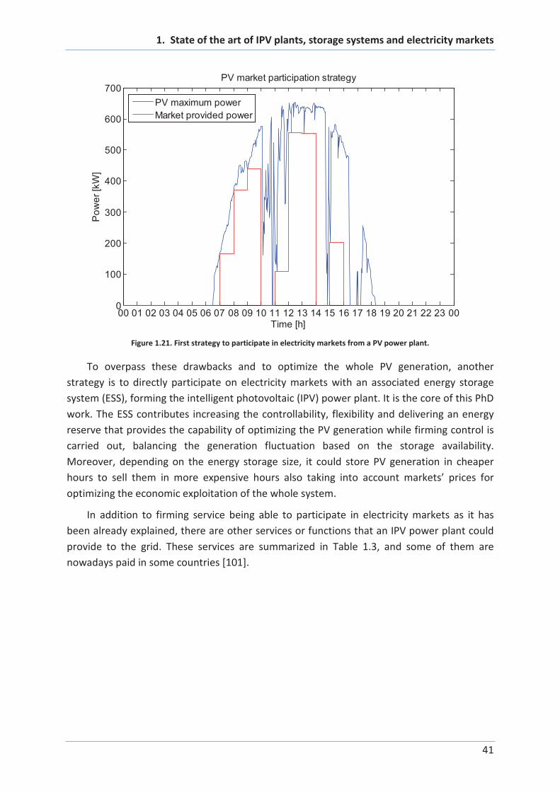
1. State of the art of IPV plants, storage systems and electricity markets
41
Figure 1.21. First strategy to participate in electricity markets from a PV power plant.
To overpass these drawbacks and to optimize the whole PV generation, another
strategy is to directly participate on electricity markets with an associated energy storage
system (ESS), forming the intelligent photovoltaic (IPV) power plant. It is the core of this PhD
work. The ESS contributes increasing the controllability, flexibility and delivering an energy
reserve that provides the capability of optimizing the PV generation while firming control is
carried out, balancing the generation fluctuation based on the storage availability.
Moreover, depending on the energy storage size, it could store PV generation in cheaper
hours to sell them in more expensive hours also taking into account markets’ prices for
optimizing the economic exploitation of the whole system.
In addition to firming service being able to participate in electricity markets as it has
been already explained, there are other services or functions that an IPV power plant could
provide to the grid. These services are summarized in Table 1.3, and some of them are
nowadays paid in some countries [101].
00 01 02 03 04 05 06 07 08 09 10 11 12 13 14 15 16 17 18 19 20 21 22 23 000
100
200
300
400
500
600
700
Time [h]
Po
we
r [k
W]
PV market participation strategy
PV maximum power
Market provided power

1. State of the art of IPV plants, storage systems and electricity markets
42
Table 1.3: Possible functions that an IPV power plant could provide to the grid [101].
Possible functions that an IPV power plant could provide to the grid
Arbitrage Frequency control or
primary control Black-start
Power shifting Inertia emulation Power quality improvement
Filtering or firming Power oscillation damping Load leveling/peak shaving
Voltage control or var
regulation Islanded mode operation Demand side management
The most representative or usual ones are: the frequency control or primary control
service which is referred to primary frequency regulation; the voltage control or var
regulation which operates similarly but injecting or absorbing reactive power for controlling
the voltage value; the power shifting service which is used to shift the production profile and
to match the demand curve; the power quality improvement service which reduces the
production fluctuations as well as unbalances and distortions, filtering the output profile of
the generator or producer; and the firming or filtering service, which makes the output
profile constant for participating in the electricity market.
Some of these functions or services demand a low power and energy requirements, and
some other ones demand greater power and energy requirements. For that reason,
depending on the objectives (functions or services) for the desired application, it is necessary
to consider the benefits obtained due to increasing the size of the storage (providing more
services) counteracted with the extra costs assumed by that system. Once weighted up
these mentioned issues, the sizing of the ESS has to be carried out, also taking into account
the most appropriate storage technology. Nevertheless, it is known that the storage system
capacity cost is the most expensive part of the whole IPV power plant, and for that reason it
will not be viable to construct an IPV power plant with a huge storage system to provide
services of big amounts of energy as secondary or tertiary regulation. The same reason
cancels the purely arbitrage service: buying cheap energy for storage and selling expensive
energy from the ESS.
Considering the above explained possible services operation, several projects of IPV
power plants are being developed as demonstrators all over the world. These demonstrators
are developed for showing the usefulness of participating in different markets and services
as represented in the Table 1.4. In this review, not only the PV power plants are analyzed,
but also a possible combination of wind power with storage systems (named IWP) due to the
drawbacks of the PV fluctuations and predictions difficulties also happening with the wind
power. Location, battery energy storage system technology, application and provided

1. State of the art of IPV plants, storage systems and electricity markets
43
services are included in this review presented in the Table 1.4, where all included systems
are experimental installations.
Table 1.4: Relevant experimental RES + BESS installations summary.
Relevant experimental RES + BESS installations
Project Location BESS
Technology Application Provided services
PNM Prosperity
Energy Storage
Project [102]
New Mexico,
USA
Adv. lead acid
and
ultrabatteries
IPV
BESS (750 kW /
2.8 MWh)
PV (500 kW)
Voltage control, power shifting and
peak shaving
ILIS Project [13, 14] Navarre,
Spain Lithium-ion
IPV
BESS (1 MW /
560 kWh)
PV (1.2 MW)
Firming, voltage control, frequency
control and ramp rate control
Kaua’I Island Utility
Cooperative (KIUC)
Project [17]
Hawaii, USA Adv. lead acid
IPV
BESS (1.5 MW /
1 MWh)
PV (3 MW)
Firming and frequency control
Wakkanai Mega
Solar Project [16]
Wakkanai,
Japan
Sodium sulphur
(NaS)
IPV
BESS (1.5 MW /
11.8 MWh)
PV (5 MW)
Firming and short term fluctuation
reduction (filtering or firming)
National Wind and
Solar Energy
Storage and
Transmission
Demonstration
Project (I) [103]
Zhangbei,
China Lithium-ion
PV + WP + BESS
BESS (6MW /
36MWh)
WP (100 MW)
PV (40 MW)
Power shifting and firming
Tehachapi Wind
Energy Storage
project [104, 105]
California,
USA Lithium-ion
IWP
BESS (8MW /
32MWh)
WP (660 MW)
Power shifting, firming and
frequency and voltage regulation
Kaheawa Wind
Power Project II
[106]
Hawaii, USA Adv. Pb acid
IWP
BESS (10MW / 7.5 MWh)
WP (21 MW)
Power shifting, firming, reserve capacity and frequency and
voltage regulation
Rokkasho-
Futamata Wind
Farm [107]
Rokkasho,
Japan Sodium sulphur
(NaS)
IWP
BESS (34MW / 238MWh)
WP (51 MW)
Power shifting, firming, load leveling and spinning reserve
AES Laurel
Mountain Wind
Farm [108]
West
Virginia, USA Lithium-ion
IWP
BESS (32 MW / 8MWh)
WP (98 MW)
Power shifting and firming

1. State of the art of IPV plants, storage systems and electricity markets
44
As it can be confirmed from the Table 1.4, most of the installations have the firming
capacity, which is the most important function for participating in the electricity markets.
Moreover, several demonstrators have also the frequency and voltage regulation control
which is a payment service in some countries as USA [109], and is a necessary service in
islanded regions as Japan, Hawaii or Puerto Rico [110-113]. In this last one, a new energy
storage mandate was signed that requires a 30 % of minimum storage capacity for any new
grid-connected solar and wind power projects to help with the control of the frequency
[113]. In Chile, the government is introducing a requirement of 7 % of power reserve, which
is only feasible by introducing ESS to renewable power plants [114, 115]. In French islands
also a mandatory regulation requires at any time of the day that the uncontrollable
electricity generation (wind and PV) never exceeds 30 % of the overall electricity
consumption [116]. For that reason, in 2012 the French Electricity Regulation Commission
(CRE) selected some projects to install more reliable wind generation systems to provide
some ancillary services based on storage systems [51].
Another possible control that the renewable generators with storage can provide is the
ramp rate control. The regulation of some countries imposes nowadays ramp rate limits
[111, 112, 117, 118]. It is the case of islands or weak grids regions. This fact forces to include
storage systems in those regions to enable the connection of renewable generation plants.
For that reason, the ramp rate control is a very common research topic of the renewable
power plants with storage systems [14, 25, 119-122].
Thus, the perspectives about renewable generators are that these types of sources must
also operate as other traditional generators, participating in current electricity markets with
current laws. To do so, it is necessary to develop operation strategies to maximize the
economic exploitation of these systems. In that perspective, most interesting markets are
the daily market and the intraday market. The daily market operation is the most beneficial
one because the overall PV generation could be cleared in this market requiring a relatively
low amount of energy capacity to provide the firming service. The intraday market is as
beneficial as daily market when palliating erroneous predictions for example. Services that
require a huge amount of energy (secondary or tertiary regulation) are not viable due to the
heavy cost of the storage system. Other services, such as inertia emulation or primary
control of frequency could be provided but are negligible in terms of energy for the storage
system because they need a low amount of energy [25].
1.5. Conclusions
The conclusions of the analysis of the state of the art are focused on summarizing the
main lacks found in the topics that are part of the present application. Therefore, the
possible improvements detected within this analysis will serve as basis to the developments
proposed in this PhD work.

1. State of the art of IPV plants, storage systems and electricity markets
45
Analyzing the first section about power architectures, one of the conclusions is that,
depending whether the IPV power plant is constructed from a given PV power plant or not,
the optimal power architecture can differ. Moreover, the possible introduction of
supplementary converters has an influence on the cost of the whole system, while also
providing some complementary controllability level. Consequently, the configuration of the
storage system in the power architecture is considered as another parameter to take into
account in the present study and there is not an optimal architecture for all cases. Thus, the
optimal power architecture depends on the original PV power plant and the desired level of
controllability. As the considered IPV power plant as case study is a real IPV power plant
located in Navarre (Spain), the configuration selected for the present PhD is the one of this
IPV power plant where the storage system is a centralized system connected to an AC
connection mode.
Regarding the control structure, the first and easiest conclusion is that the management
layers must be separated to have an easier view of different control layers and the objective
of each of them. Thus, different conclusions must be drawn about the energy management
layer and the power control layer. The number of works related to researches in the energy
management layer is limited for the IPV application at grid scale due to the innovation to
participate in electricity markets, accepting that a long-term horizon must be taken into
account in that case, and that the storage system plays an important role in the capacities of
the management. Nevertheless, there are several works about the energy management
layer for wind power applications, which offer an idea of the services that could be
integrated in this management layer [49-52, 54, 55]. To counteract this lack of works about
energy management of IPV power plants, advanced energy management strategies are
developed and are presented in later chapters as main contribution of the scientific
community through this PhD.
Analyzing the power control layer, several works have been carried out, changing the
maximum power point of the PV converters, but from the scope of this PhD work, the power
control layer focuses more on the rapid ancillary services. On this aspect, the main
conclusion of the power control layer is that the IPV power plant is able to participate in
some services as frequency and voltage regulation, inertia emulation, power oscillation
damping, power fluctuation reduction and ramp rate control. Therefore, the combination of
the centralized power plant controller explained in [14], with the predictive control constant
steps value of [27, 53], could achieve a well performing power management layer, also
considering the higher level of the energy management. In this predictive control, some
other criteria and constraints could be included in order to improve the general
management structure.
As a conclusion of the energy storage system and its sizing, the technology selection is
defined as one important milestone which determines the possibility to provide some
services or another ones, as well as balances the economic exploitation of the whole IPV

1. State of the art of IPV plants, storage systems and electricity markets
46
system. For that reason, a technology selection methodology is developed in this PhD work
and will be presented in the next chapter.
Related to the sizing methods review, it must be underlined that most of the cited
authors have shared that the economic viability of the integration of an energy storage
system is not clear in most renewable applications. Nevertheless, in the present work and
taking into account energy policies that allow the participation of the IPV power plants in the
electricity markets and providing ancillary services, the storage system could help or
collaborate in the augmentation of the massive integration of the renewable energy sources.
For obtaining the desired economic viability of the IPV power plant system, the balance
between the sizing of the storage system and the operation strategies to correctly use this
storage system is essential. Thus, a combined optimization that calculates the best storage
system together with the most interesting operation strategy to obtain the optimal
economic exploitation is carried out in the present PhD.
This operation strategy is based on the electricity markets’ analysis, showing that
nowadays the most interesting markets to participate in are the daily and the intraday
markets. With the developed combined optimization mentioned before, some innovative
market participations are proposed, which maximize the economic exploitation, reducing
the PV uncertainties through a participation in the intraday markets. This market
participation follows the perspectives about renewable generators, which states that these
types of sources must also work as other traditional generators, participating in the current
electricity markets with current laws.

2 IPV power plant
description and
modeling


2. IPV power plant description and modeling
49
2. IPV power plant description and
modeling
The objective of this second chapter is to detail the IPV power plant features in order to
be able to carry out their modeling issues. As it has been previously verified in the section
where the experimental RES + BESS installations have been presented, the storage system
size and its technology have to be selected, depending on the services or functions to be
provided. For that reason, there are two questions that must be answered which are: “What
is wanted to do?” which refers to the functions or services that are required to the given
power plant; and the second question is “How is it going to be done?” referring to the
technology and the size of the storage system.
As it has been introduced before, the main objective of the present PhD is to develop an
electricity market participation process, and therefore, the first question has already been
answered. In this chapter, the second question related to which technology is going to be
selected will be answered. To do so, a technology selection methodology is developed. This
methodology analyzes the services that have to be provided to different grid levels, to finish
selecting the correct technology for its following integration.
Once the technology has been chosen, the case study IPV power plant is presented and
described. Finally, the modeling of the different IPV power plant agents is carried out
considering the electric and economic models of the PV field; the energetic, degradation and
economic models of the storage system; the electricity market model; and the IPV power
plant model.
2.1. Storage technology selection methodology
Taking into account the several parameters of the storage systems, a technology
selection methodology is developed and proposed. This methodology is presented in [66].
First of all, a storage system can be installed in different locations of the whole electricity
network: at the generation systems, at the T&D (transport and distribution), at the end-user
and at the RES connection point. At each location, the functionalities that the storage system
can provide are different and can be summarized in [66]. In the present work, the most
relevant grid level is the RES integration. For that reason, once the relevant experimental
RES + BESS installations have been summarized (Table 1.4 of Chapter 1.4.3), it can be stated
that the most installed BESS technologies are lithium-ion batteries (Li-ion), sodium sulphur
batteries (NaS) and advanced lead acid batteries (adv. Pb acid).
Not only technical criteria must be taken into account to determine which of these three
technologies is the most adequate one for RES integration. Therefore, other criteria are
included to select the most suitable technology.
2. IPV power plant description and modeling
50
2.1.1. Considered technical and economic criteria
The considered technical and economic criteria for the following comparison are
described below. These criteria are considered to be the most representative ones for the
present application. Nevertheless, if the application requires it, other criteria could be
included. Some of them are the technical ones explained in the previous chapter (Section
1.3.2), but are also included here to list both technical and economic criteria.
1) Power to energy ratio [kW/kWh]: It describes the ratio between power and
energy.
2) Energy density [Wh/m3]: It represents the available energy per volume unit.
3) Energetic efficiency [%]: It shows the relation between the discharged energy and
the amount of energy needed to restore the initial charge state, under specific
conditions. It is measured in percentage.
4) Life cycles [cycles]: It determines the quantity of consecutive charge and discharge
processes that a battery can undergo while maintaining some minimum
performances.
5) Calendar life [time]: It determines the period of time in which the battery
maintains some minimum performances without being used.
6) Capital cost & BMS cost [€/kWh]: It represents the cost of the BESS with its BMS
(Battery Management System) incorporated.
7) Maintenance cost [€/kWh]: It represents the cost of maintenance of the BESS in
order to assure some specific performances.
8) Commercial maturity: It indicates the period of time in which the technology has
been in use and the development experienced in that period.
9) Security: It represents the safe operation range of the BESS.
2.1.2. Value assignment for each criterion and comparison of
technologies
Based on the described criteria, Li-ion, NaS and adv. Pb acid technologies are compared
in detail. The results of the comparison in terms of value assignment of criteria are depicted
in the spider chart of Figure 2.1.

2. IPV power plant description and modeling
51
Figure 2.1: Spider chart of relevant BESS technologies comparison.
1) Power to energy ratio [kW/kWh]: Li-ion technology (~15 kW/kWh) has the
highest power to energy ratio, much higher than the one of the adv. Pb acid (~5
kW/kWh) and NaS technologies (~2 kW/kWh) [68, 123].
2) Energy density [Wh/m3]: The Li-ion has the greatest energy density (200-350
Wh/m3) followed by NaS technology (150-250 Wh/m3). Adv. Pb acid technology
has the lowest energy density value (50-100 Wh/m3) [61].
3) Energetic efficiency [%]: The Li-ion has the greatest efficiency with 90-94%,
followed by the adv. Pb acid (75-90%) and the NaS (75%) [124].
4) Life cycles [cycles]: Li-ion and NaS technologies have similar life cycles around
5000 cycles and adv. Pb acid technology has approximately a durability of 1000
cycles [124, 125].
5) Calendar life [time]: The NaS has the best calendar life (15-20 years) followed by
Li-ion (5-20 years depending on temperature and SOC) and by adv. Pb acid (5-15
years depending on temperature and SOC) [68].
6) Capital cost & BMS cost [€/kWh]: Li-ion batteries are the most expensive ones. So
they have the lowest value in this criterion followed by NaS technology. Adv. Pb
acid technology is much cheaper than other technologies having the best score
[61, 126].
7) Maintenance cost [€/kWh]: NaS batteries have the most expensive maintenance
cost, due to their high operation temperature. This technology is followed by Li-
ion and adv. Pb acid technologies, which require little maintenance. Thus, the
lowest score is for NaS, followed by Li-ion and adv. Pb acid [127].
EESS technologies comparison
510
Power to energy ratio
5
10
Energy density
5
10
Energy efficiency
5
10Life cycles
5
10
Calendar life
5
10
Capital cost & BMS cost 5
10
Maintenance cost
5
10
Commercial maturity
5
10Security
Li-ion
NaS
Adv. Pb acid

2. IPV power plant description and modeling
52
8) Commercial maturity: The NaS is the most mature technology and Li-ion and adv.
Pb acid technologies are still in demonstration stage [128].
9) Security: The adv. Pb acid is the most secure technology followed by Li-ion and
NaS technologies [68].
In conclusion, as it can be observed in Figure 2.1, there is not a technology that prevails
over the others at all criteria. The comparison between the arithmetic additions of criteria’s
values shows that Li-ion is the best positioned technology. However, for a specific
functionality, some characteristics are considered to be much more important than others,
i.e. the security characteristic in transport applications (trains, electric vehicles, planes). As a
result, this arithmetic addition could not be enough to select a battery energy storage
technology. In order to rate the importance of some BES characteristics for a specific
application a new selection methodology is proposed in this PhD work and is presented as
follows.
2.1.3. Description of the proposed methodology
The objective of the proposed methodology is to offer the possibility to rate the
importance of some BES characteristics for the specific application where the methodology
is applied. The methodology is based on the flowchart depicted in Figure 2.2.
The first step of the methodology consists in defining the main aspects of the
application where the BESS will be installed. These aspects include, among others, the
energetic and location requirements, specific legal regulations, functionality to be provided,
etc. The second step includes the numerical identification of the above described criteria for
each considered BES technology. The third step contains the weigh up value assignment for
each criterion. This assignment process will be done based on the analysis of the application
of the step 1. The following step calculates each technology qualification applying Eq. 2.1.
= 1( ) + 2( ) + 3( ) +
4( ) + 5( ) + 6( ) & +
7( ) + 8( ) + 9( )
Eq. 2.1
Where:
( ) is the weigh up value of the functionality for the criterion. The sum of all
values for each functionality must be 100, so each criterion has a weigh up
value between 0 and 100. It must be noticed that if a given ( ) value
increases over 11.11 (which represents the equitable weighting value as it can
be verified in Table 1.1), another value must decrease.
is the value of each criterion for each technology, with a value between 0 and
10. These values can be obtained from the spider chart of Figure 2.1.

2. IPV power plant description and modeling
53
The result of this equation will be a value up to 900 because there are 9 criteria
multiplied each one by the functionality weigh up value. The higher the value, the better is
the technology. The different qualifications obtained for the different BES technologies are
then compared to select the best technology for the considered application. By replacing the
coefficients Kx of each criterion by cost values, equation (Eq. 2.1) could also represent a cost
equation. In that case, the lower the value, the better is the corresponding technology.
Figure 2.2: BES technologies selection methodology flowchart.
2.1.4. Application of the proposed methodology
For demonstrating the usefulness of the methodology, its application is presented in this
section. The considered case study is a 500 kWh/1MW BESS for RES integration functionality.
The following requirements are defined for the application:
Country legal regulations demand a high security installation.
In order to follow green politics an efficient installation is required.
The cost factor is considered to be very important.
It is considered that the RES integration functionality requires a high power to
energy ratio for high peak power response.
Based on those requirements, among the technical and economical characteristics
identified in section 2.4.1.1, the most important criteria for this application are the security,
the energetic efficiency, the capital cost and the BMS cost, the power to energy ratio and the
life cycles (since it affects on the replacement cost). These criteria are weighed up with a
15% value. In terms of importance, the next family criteria are considered to be the
commercial maturity with a weigh up value of 10%. The other characteristics that are the
calendar life, the maintenance cost and the energy density, which are less relevant in this
application, are weighed up with a 5% value. These values for different criteria are depicted
Application
analysis
Weight value
assignment
Equation result
interpretation:
technology election
iaaa ,...,, 21
SeciEnDenPErat KaKaKaQual ...21
321 TechTechTech QualQualQual
Identification of
criteria values SecEnDenPErat KKK ,...,,
identification
- energetic requirement
- location needs
- legal regulations
- ….
- functionality to provide

2. IPV power plant description and modeling
54
in Table 2.1. The defined values are compared with the values obtained by applying the
equitable weighting.
Table 2.1: Weigh up value table with equitable weighting and for RES integration functionality.
Weigh up
value
Technical and economic
criteria
Equitable
weighting
RES
integration
functionality
1( ) Power to energy ratio 11.11 15
2( ) Energy density 11.11 5
3( ) Energetic efficiency 11.11 15
4( ) Life cycles 11.11 15
5( ) Calendar life 11.11 5
6( ) Capital and BMS cost 11.11 15
7( ) Maintenance cost 11.11 5
8( ) Commercial maturity 11.11 10
9( ) Security 11.11 15
( ) Total 99.99 100
Considering the weigh value assignment in Table 2.1 (corresponding to the equitable
weighting for one and a customization for RES integration for the other one) the proposed
methodology is applied and the results obtained are shown in Table 2.2.
Table 2.2: Methodology application results for equitable weighting and for RES integration functionality.
Technologies Li-ion NaS Adv. Pb acid
Results
Equitable weighting
789 (87.65%)
633 (70.36%)
744 (82.71%)
RES integration functionality
765 (85.00%)
615 (68.33%)
755 (83.89%)
Applying the equitable weighting, the Li-ion technology (789 – 88%) is much better than
the others with a significant margin, 5% respect to adv. Pb acid (744 – 83%) and 18% respect
to NaS technology (633 – 70%). The difference of the adv. Pb acid is due to its low energy
density and power to energy ratio values, which are counteracted in part by its low capital

2. IPV power plant description and modeling
55
cost and high security. Concerning the NaS technology, the main reason of the difference
comes from its low security and high maintenance cost.
Applying the weighting defined for the RES integration functionality, the best
qualification is also for the Li-ion technology (765 – 85%) but with a lower value than the
previous case. This is due to the high capital cost and the BMS cost of the Li-ion that
considerably influences the qualification. It must be noticed that the adv. Pb acid technology
(755 – 84%) has increased its qualification value, due to its low cost and high security levels.
The NaS technology qualification value (615 – 68%) has decreased. Its qualification is even
further from the other two technologies because of its low security and high cost which
make it more penalized.
These results confirm the choice adopted in the experimental installations of Table 1.4
(Section 1.4.3), where for the RES integration, the most applied technologies are the Li-ion
and the adv. Pb acid technologies. Nevertheless, for the present PhD study one of these two
technologies must be selected. For that reason, the lithium-ion, which is the best qualified
technology, is selected as the storage system technology for the present PhD work.
Regarding the current available worldwide energy storage systems, one third of them are
based on lithium-ion technology [59] and therefore the selection of lithium-ion is confirmed
as a correct selection.
2.2. Case study system description
As a case study of an IPV power plant, a real plant located in Tudela, Navarre, Spain, is
considered. This power plant is owned by Acciona Energía [35]. Nevertheless, Ikerlan has
participated in a project (ILIS project[14, 129, 130]) to convert this PV power plant in an IPV
power plant, installing a BESS. The connection configuration of the BESS to the PV power
plant is by means of a centralized storage system connected in AC mode. Thus, the
considered system is this real plant, which is detailed in this section.
The considered system is a 1.2 MW PV power plant. The plant covers an area of 70000
square meters and the solar radiation of its location is 1600 kWh/(m2·year). This power plant
was constructed in 2001. Its aerial picture is presented in Figure 2.3.

2. IPV power plant description and modeling
56
Figure 2.3: Aerial picture of the PV power plant located in Tudela, Navarre, Spain [14].
2.2.1. Power architecture
The power plant is separated in two areas: a 700 kW / 865.8 kWp centralized generation
area and a distributed generation area with 300 kW / 321.11 kWp installed PV power.
The centralized generation area represents 70 % of the PV plant and it is composed of
280 trackers, each one with 36 PV panels in series connection mode. The 10080 PV panels
that compose this area are the model BP 585 monocrystalline photovoltaic modules of BP
Solar [131]. The 280 trackers generation is connected forming 7 controllable generation
units. Each of them, with a peak power of 122.4 kWp, is connected to the internal 380 VAC
network by a 100 kW power electronics converter (Voltage source converter, VSC).
The distributed area is composed by 11 types of PV panels of nine manufacturers and
five technologies, with a total of 2522 PV panels. This area is considered as a single
generation unit without energy management capability and also connected to the internal
380 VAC network.
The PV generation is connected to the medium voltage by a 380 V / 20 kV transformer
inside the PV plant and to the transmission system (66 kV) through another transformer
located in a substation also owned by Acciona at 2 km from the PV plant.
This configuration was restructured in 2012 in the framework of a European Union
supported ILIS project [129, 130], including a storage system and a centralized plant
controller to adapt the PV plant to the new interconnection requirements and to
experimentally test them as it is explained in [14]. The configuration of this IPV power plant

2. IPV power plant description and modeling
57
is presented in Figure 2.4. This configuration was only in operation between 2012 and 2013,
in the framework of the mentioned European project.
380 V 20kV 66kV
Grid
20kV
DC
AC
100kWPV6
DC
AC
Local controller
300kWDistributed
PV
PLANT
CONTROLLER
AC
DC
Battery localcontroller
BMS
PCC
1MW Battery
communications
PV6 Local controller
DC
AC
100kWPV7
PV7 Local controller
DC
AC
100kWPV5
PV5 Local controller
DC
AC
100kWPV4
PV4 Local controller
DC
AC
100kWPV3
PV3 Local controller
DC
AC
100kWPV2
PV2 Local controller
DC
AC
100kWPV1
PV1 Local controller
IPV power plant
Figure 2.4: Configuration of the IPV power plant (in operation between 2012 and 2013).
The included storage system was a Lithium-ion battery of 1 MW / 560 kWh of SAFT, as it
can be shown in Figure 2.5. This storage system was composed by 10 parallel battery strings,
each of them built by 29 battery modules. Its nominal voltage was 730 V.

2. IPV power plant description and modeling
58
Figure 2.5: Picture of the installed lithium-ion battery of 1 MW / 560 kWh of SAFT [14].
The storage system was connected to the internal network through a 1 MW power
electronic converter (VSC). The centralized plant controller carried out the IPV power plant
level control and the communications with all lower level controllers of the facility. The
existing communications can also be seen by means of the red dashed lines of Figure 2.4.
2.2.2. Control architecture
Related to the control architecture, it is important to mention that the IPV power plant
has a hierarchical structure. The higher level controller, which is the plant controller,
controls the power injected into the grid measured at the PCC. Based on these
measurements, the plant controller sends the needed references to the lower level
controllers. These communications are carried out by standard communication protocols.
Each of those lower level controllers (which are all of the controllable PV generation units,
the converter of the storage system and the storage system itself) have their own local
controller, as it can be verified in yellow rectangles in Figure 2.4.
The PV local controllers can be controlled in two different ways: in MPPT mode (where
the objective is to extract the maximum power from the sun irradiation) and in PQ mode
(where the defined active and reactive power set-points of the higher level plant controller
are followed). The battery local controller was controlled in PQ mode and the BMS (Battery
Management System) provided information to the plant controller related to the battery,
like the state of charge. The plant controller carried out the regulation of the active and
reactive power injected to the grid at the PCC. For doing so, it had two modules which were
the control module and the dispatch module as it can be shown in Figure 2.6.

2. IPV power plant description and modeling
59
Plant PQ
control
module
PQ dispatch
module
Plant controller
System
operator
demands
P references
Q references
PV generation
ESS generation
measurementsPCC
Figure 2.6: Internal control blocks of the plant controller [14].
Plant PQ control module: this module contains the active and the reactive power
control loops based on PI controllers. They assure that the global power references received
from the system operator are reached at the PCC. These references are calculated taken into
account the estimated available PV power and the ESS reserves. Several grid functionalities
or services as frequency regulation, voltage regulation, ramp rate control or firming control
(constant power production) are implemented in this module.
PQ dispatch module: this module distributes to the controllable PV systems and the
storage system the calculated references of the before explained module. It has two
different dispatching strategies that are dependent to the PV power availability and the SOC
of the storage system. Each strategy is explained in the Table 2.3.

2. IPV power plant description and modeling
60
Table 2.3: PQ dispatching strategies.
Mode 1: IPV plant control without ESS Mode 2: IPV plant control with ESS
This mode can be activated when there
is no storage system or when it is not
available.
Only the PV controllable units
participate in the plant control.
Both PV controllable units and the
BESS participate in the plant control.
Depending on the SOC of the storage
system, PV controllable units operate
in MPPT mode or in PQ mode.
Mode 1 dispatching equations: Mode 2 dispatching equations:
In MPPT mode:
= Eq. 2.2 = Eq. 2.3
= Eq. 2.4 = Eq. 2.5
= 0 Eq. 2.6 = Eq. 2.7
= 0 Eq. 2.8 = Eq. 2.9
Where:
= 1, … ,7 = 7
Where:
= 1, … ,7 = 8 = 7( ) + 1( )
In PQ mode:
= = Eq. 2.10
= = Eq. 2.11
Where:
= 1, … ,7 = 8 = 7( ) + 1( )
System
operator
demandsPLANT CONTROLLER
PCC
measurements
PV1
PV2
PV3PV4
PV5
PV6
PV7
PV local controller
Power
references
PV power generation
System
operator
demandsPLANT CONTROLLER
PCC
measurements
PV1
PV2
PV3PV4
PV5
PV6
PV7
PV local controller
Power
references
PV power generation
ESS
Battery localcontroller
Power
reference
ESS exchanged power
Figure 2.7: Mode 1 dispatching strategy. Figure 2.8: Mode 2 dispatching strategy.

2. IPV power plant description and modeling
61
The selected dispatching strategy is the Mode 2, which considers the storage system
taking advantage of its energy reserves. Among those two operation modes, the MPPT mode
is the principal one, because it optimizes the PV generation while controlling the IPV output
power by the storage system flexibility. Nevertheless, the PQ mode and the first strategy
(without ESS) provide more flexibility to the whole plant for the cases when the SOC of the
storage system is near its limits or when there is some kind of problems with the storage
system (as communication errors, for example).
As it has been mentioned before, the ESS was in operation between 2012 and 2013, in
the framework of the European project, but the centralized plant controller continues today
in operation, managing the whole PV power plant with the developed control architecture.
Nevertheless, the present PhD work has been developed assuming the scenario where an
ESS is connected to the PV power plant, considering then an IPV power plant.
2.3. IPV agents modeling
This section includes all modeling steps of each device or agent of the IPV power plant.
As the main objective of the present work is to determine the required energetic capacity of
the storage system in order to take advantage of it to participate in the market, the energy
storage model is an energetic model, which means taking into account its power and energy
values, more than voltage and current values (parameters of an electric model). The
economic models of these devices are also considered and explained in this section, as well
as the degradation model of the storage system.
2.3.1. PV model
The considered PV models are the electric and the economic ones. They are developed
as follows:
2.3.1.1. Electric model
The electric model applied in this study is an energetic one, which means that the
output power of a PV subsystem (PV panel + converter) is considered. The PV generation
data taken into account is a one yearlong and two minutes sample time generation data [26]
(which do not represent real data from Tudela) of the generated kilowatts per installed
kilowatt peak value [kW/kWp]. This data is, therefore, the generated power at the converter
output in per unit of installed peak power ( [ ]) and it is presented in Figure
2.9.
From this data, the output power generation of a given PV power plant is easy to obtain,
knowing its installed PV peak power. As the experimental validation of the present PhD is
done based on a real PV power plant, the model of this plant is considered to determine the
output power generation. The mentioned PV power plant has 1.2 MWp installed capacity.
Therefore, its output power generation is calculated as in Eq. 2.12.

2. IPV power plant description and modeling
62
= [ ] = 1.2 Eq. 2.12
1 29 57 85 113 141 169 197 225 253 281 309 337 3650
0.1
0.2
0.3
0.4
0.5
0.6
0.7
0.8Real one year long PV generation profile
Time [days]
kW
/kW
p
58 59 60 610
0.1
0.2
0.3
0.4
0.5
0.6
0.7
0.8
Time [days]
kW
/kW
p
PV
dat
a[k
W/k
Wp
]
Figure 2.9: Real one year long PV generation profile with a three days detail [26].
2.3.1.2. Economic model
The economic model of the PV system includes the initial investment cost. The initial
investment cost is divided in two terms, considering the purely PV installation and its
associated power electronics (PE). Therefore, the initial investment cost of the PV
system, , is calculated as in Eq. 2.13.
= + Eq. 2.13
Where (€) and (€) are the PV panels investment cost and PV related
power electronics investment cost. Each of these costs is calculated as in Eq. 2.14 and in Eq.
2.15, respectively.
= Eq. 2.14
= Eq. 2.15

2. IPV power plant description and modeling
63
Where (W), is the installed PV power capacity and (€/W) and (€/W)
are the cost per watt of PV panels and power electronics. The considered costs are 1 €/W
and 0.1 €/W, respectively.
2.3.2. Energy storage system model
The energy storage system is detailed in three models which are the energetic model,
the degradation model and the economic model. This classification is made to take into
account the energetic capacities of the storage system, the degradation that this energetic
capacity supports and the cost caused from the degradation that concludes with a
replacement of the storage system.
2.3.2.1. Energetic model
The energetic model considered in this study calculates the state of charge ( ) of the
storage system based on Eq. 2.16 [24].
( ) =( )
( ) Eq. 2.16
Where ( ) (Wh) is the current energetic capacity and (Wh) is the current
maximum capacity. A fresh or new storage system has a nominal capacity value, , and
since this moment, the battery is degraded reducing its maximum capacity value. Therefore,
the current ( ) maximum capacity value is ( ).
Although the definition of the SOC can be calculated based on Eq. 2.16, the Coulomb
Counting technique is also very extended to calculate the SOC for each moment [132, 133].
This method is also known as Ah-counting and it carries out the integration of the current
flowing through the storage system according to Eq. 2.17.
( ) = ( 0) ( )0
Eq. 2.17
Where is the efficiency of the charge and discharge processes, which is more than 1
on discharge and less than 1 on charge; (Ah) is the nominal capacity; and ( )(A) is the
current extracted or injected to the battery over the time. This method, as its name indicates
(Ah-counting), calculates the quantity of the Ampere-hours (current during time) flow.
Nevertheless, in this study the capacity of the battery ( ) is considered in watts-hour,
instead of ampere-hour, as mentioned in Eq. 2.16. Therefore, the voltage ( ) is included as
constant value in the integration of the current, to maintain the equation units
correspondingly [134]. With this assumption, the Eq. 2.17 is used as Eq. 2.18 in this study.
( ) = ( 0)( )
( ) 0
= ( 0)( )
( ) 0
Eq. 2.18

2. IPV power plant description and modeling
64
Where (W) is the power exchanged with the battery. The discrete equation of Eq.
2.18 is presented in Eq. 2.19.
( ) = ( 0)( )
( )
= 0
Eq. 2.19
Where (h) is the sample time counted in hours. As it can be shown in Eq. 2.19, the
SOC is a recursive parameter, which means that it is related to its previous values. As in Eq.
2.19, the SOC value of the previous sample time, ( 1), is calculated as in Eq. 2.20.
( 1) = ( 0)( 1)
( )
1
= 0
Eq. 2.20
Combining Eq. 2.19 and Eq. 2.20, and assuming that the capacity decay is negligible
between two continuous steps ( ( ) ( 1) 0), a simplified equation of the
SOC can be obtained (Eq. 2.21), which calculates the current SOC only with the information
of the previous step, which reduces the calculation time. This Eq. 2.21 is the one that is used
in the present study.
( ) = ( 1)( )
( ) Eq. 2.21
2.3.2.2. Degradation model
At the present PhD study, a degradation model is also considered to take into account
the battery capacity reduction. To do that, the state of health ( ) of the battery is
calculated as in Eq. 2.22.
( ) =( )
Eq. 2.22
Where ( ) (Wh) is the current maximum capacity and (Wh) is the capacity of
the battery in its beginning of life (BOL), which means when it is fresh or new battery.
The ageing in storage systems refers to a reduction of the amount of energy that the
batteries are able to provide and also to an internal impedance increase. Therefore, when
there are degraded, they are able to provide lower amount of energy within lower power
values. This degradation is caused by two factors: the cycling ageing and the calendar ageing.
The cycling ageing is modeled as in [24] assuming that the capacity losses are linear
according to the discharges of the storage system [135-139]. That means that at each
discharge, there is a capacity loss. This fact is modeled in a discrete domain as in Eq. 2.23.
( ) = ( 1) ( ) at each discharge step Eq. 2.23

2. IPV power plant description and modeling
65
Where (Wh) is the capacity loss of the step . This capacity loss is calculated as in
Eq. 2.24.
( ) = ( 1) ( ) Eq. 2.24
Where is the linear ageing coefficient. This coefficient has different values for
different storage systems’ technologies [137]. For lithium-ion batteries this coefficient has a
1,1 10 3 value [26].
Overwriting the Eq. 2.22 in the discrete domain, the resultant equation is Eq. 2.25 or Eq.
2.26 for different time steps.
( ) =( )
Eq. 2.25
( 1) =( 1)
Eq. 2.26
Replacing Eq. 2.23 in Eq. 2.25 and applying there the Eq. 2.26, Eq. 2.27 is obtained:
( ) =( )
=( 1) ( )
= ( 1)( )
Eq. 2.27
Finally, replacing Eq. 2.24 in Eq. 2.27, the cycling ageing equation (Eq. 2.28) is obtained:
( ) = ( 1)( 1) ( )
= ( 1) ( 1) ( ) Eq. 2.28
As it is aforementioned, this equation models the discharge processes and therefore, by
means of the model applied, in the charge processes the capacity and the values are
maintained constant [24]. Thus, the equation that models all cases is expressed by Eq.
2.29.
( ) =( 1) ( 1) ( ) ,
( 1), Eq. 2.29
An example of the real cycling ageing can be shown in Figure 2.10, where 6 same
battery cells are tested with different conditions: 25 ºC, 50% middle SOC, 1C (C-rate), and
different DOD (depicted in the legend) [140]. The full equivalent cycles (FEC) are counted on
each cycling test.
Once the capacity ( ( )) or the reference ( ) value cross the end of life (EOL)
threshold ( ), it is considered that the storage system is not useful for the current
application.

2. IPV power plant description and modeling
66
Figure 2.10: Example of cycling ageing for six different DOD [140].
Related to the calendar ageing, it is considered as linear ageing but in this case between
the beginning of life (BOL) and the EOL of the batteries. It is known that the calendar ageing
is dependent on the temperature, the SOC and the time of storage [141], but the
approximation carried out in this work is the linear one.
An example of the real calendar ageing can be shown Figure 2.11, where another 6
same battery cells are stored with different temperature and SOC conditions [141].
Figure 2.11: Example of calendar ageing for different conditions [141].
Based on a linear equation, the coefficients that model this ageing process can be
obtained as in Eq. 2.30.
75
80
85
90
95
100
0 1000 2000 3000 4000 5000 6000 7000
SO
H [
%]
FEC
5% DOD, 1C10% DOD, 1C30% DOD, 1C50% DOD, 1C60% DOD, 1C100% DOD, 1C
75
80
85
90
95
100
0 100 200 300 400 500 600 700
SO
H [
%]
Storage time [days]
30ºC, 70% SOC40ºC, 30% SOC40ºC, 70% SOC40ºC, 90% SOC50ºC, 70% SOC50ºC, 90% SOC
or
or
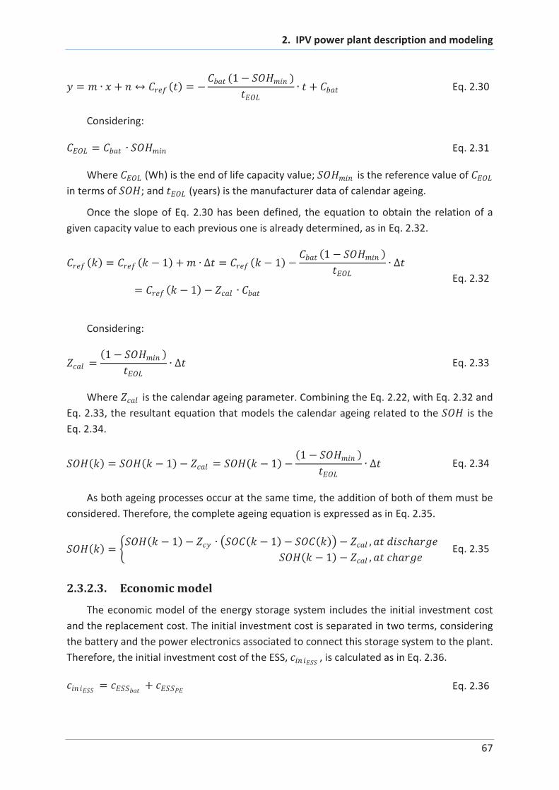
2. IPV power plant description and modeling
67
= + ( ) =(1 )
+ Eq. 2.30
Considering:
= Eq. 2.31
Where (Wh) is the end of life capacity value; is the reference value of
in terms of ; and (years) is the manufacturer data of calendar ageing.
Once the slope of Eq. 2.30 has been defined, the equation to obtain the relation of a
given capacity value to each previous one is already determined, as in Eq. 2.32.
( ) = ( 1) + = ( 1)(1 )
= ( 1) Eq. 2.32
Considering:
=(1 )
Eq. 2.33
Where is the calendar ageing parameter. Combining the Eq. 2.22, with Eq. 2.32 and
Eq. 2.33, the resultant equation that models the calendar ageing related to the is the
Eq. 2.34.
( ) = ( 1) = ( 1)(1 )
Eq. 2.34
As both ageing processes occur at the same time, the addition of both of them must be
considered. Therefore, the complete ageing equation is expressed as in Eq. 2.35.
( ) =( 1) ( 1) ( ) ,
( 1) , Eq. 2.35
2.3.2.3. Economic model
The economic model of the energy storage system includes the initial investment cost
and the replacement cost. The initial investment cost is separated in two terms, considering
the battery and the power electronics associated to connect this storage system to the plant.
Therefore, the initial investment cost of the ESS, , is calculated as in Eq. 2.36.
= + Eq. 2.36

2. IPV power plant description and modeling
68
Where (€) and (€) are the battery investment cost and ESS related power
electronics investment cost. Each of these costs is calculated as in Eq. 2.37 and in Eq. 2.38,
respectively.
= Eq. 2.37
= Eq. 2.38
Where (Wh) is the installed battery energetic capacity; (W) is the
installed battery power capacity; (€/Wh) is the cost per watt-hour of batteries;
and (€/W) is the cost per watt of power electronics. The considered battery cost is
0.4 €/Wh and the cost of power electronics is 0.1 €/W.
As the life span of the batteries is not the same as the life span of the whole IPV power
plant, the replacement cost of the batteries is considered here. The replacement cost of the
batteries is the same as the batteries investment cost, but the difference is that this cost is
usually annualized [142]. To annualize it, the Eq. 2.39 is applied:
= (1 + )
=1
Eq. 2.39
Where (€/year) is the annualized replacement cost of the batteries; is the
number of needed replacements; is the interest rate in percentage; is the lifespan of
the storage system in years; and is the capital recovery factor, which is a factor that
permits to annualize a given cost [142]. It is calculated as in Eq. 2.40.
=(1 + )
(1 + ) + 1 Eq. 2.40
Where is the lifetime of the whole IPV power plant system in years and is the
interest rate in percentage. In this case, the lifetime ( ) is considered as 25 years and the
interest rate ( ) is considered as 2.5 %.
To determine the replacements needed ( ) and the lifespan of the storage system ( ),
the battery power profile is analyzed. From this profile, the profile is obtained to apply
the Rainflow cycling counting algorithm [143, 144].
This algorithm counts the charging and discharging cycles analyzing the profile. Its
internal process can be summarized in the following three steps [145].
First, the algorithm analyses the discharges cycles beginning from the highest SOC value
and counting from top to bottom. It analyzes the discharge curve until finding the lowest
SOC value following a continuously decreasing path. The algorithm repeats the previous
process starting from the next highest SOC value until finding the next lowest SOC value

2. IPV power plant description and modeling
69
without overlapping the previous paths. This process is repeated until all the discharges of
the SOC profile are analyzed and it is demonstrated by means of an example in Figure 2.12.
Time [s]
SO
C[%
]
SOC profileDischarge
analysis1 2 3
45
6
7
Figure 2.12: First step of Rainflow cycling counting algorithm (discharge analysis).
The second step of the algorithm is similar to the previous one but charges and
discharges are analyzed in the same way. Thus, beginning from the lowest SOC value and
following until the highest SOC value, the first increasing path is determined. This process is
repeated from the next lowest SOC value until the next highest SOC value without
overlapping previous paths. Figure 2.13 shows this second step on the same example.
Time [s]
SO
C[%
]
SOC profileCharge
analysis
5
12
3 4
67
Figure 2.13: Second step of Rainflow cycling counting algorithm (charge analysis).

2. IPV power plant description and modeling
70
The third and last step matches the discharge and charge semi-cycles completing full
cycles of the same depth of discharge (DOD) and from the same upper SOC value and lower
SOC value. Figure 2.14 presents this matching process.
Time [s]
SO
C[%
]SOC profile
Cycles with
different DODs
Discharge
analysis
Charge
analysis
Figure 2.14: Third step of Rainflow cycling counting algorithm (matching process).
Once the quantity of cycles has been obtained, these cycles are matched with the
lifetime data (specific depth of discharge, DOD, versus the number of cycles) of the
datasheet of the battery manufacturer obtaining the lifetime of the storage system [146].
The cycles are grouped ten by ten to a correct match of datasheet data versus the counted
cycles. The lifetime is calculated applying Eq. 2.41.
=1
9=1
[ ] Eq. 2.41
Where is the lifetime of the energy storage system [years]; is the number of
cycles counted of DOD group per year [cycles/year] obtained from the Rainflow cycling
counting algorithm; and is the number of cycles of DOD group that causes the EOL of
the storage system taken from the datasheet of the manufacturer and also from different
cycling tests carried out in the energy storage laboratory of Ikerlan [cycles].
The considered values are the ones depicted on Table 2.4 [146]. These values
correspond to a NMC-based 40 Ah battery cell.

2. IPV power plant description and modeling
71
Table 2.4: Considered number of cycles per DOD group [146].
DOD interval
1 0 – 15 % 70000
2 15 – 25 % 31000
3 25 – 35 % 18100
4 35 – 45 % 11800
5 45 – 55 % 8100
6 55 – 65 % 5800
7 65 – 75 % 4300
8 75 – 85 % 3300
9 85 – 100 % 2500
From the obtained lifespan of the storage system ( ) and the whole IPV power plant
lifetime ( ), the needed replacements ( ) are calculated as in Eq. 2.42.
= 1 Eq. 2.42
Where the ( ) mathematical function calculates the following positive integer value
of , in order to have an integer value of replacements.
2.3.3. Electricity market economic model
The electricity market economic model analyzed in the present PhD work includes the
revenues and the penalties that an energy producer can generate participating in the
electricity markets of the Iberian Peninsula. As it is explained in the chapter 1, the markets
where an IPV power plant can participate are the daily market and the six sessions of the
intraday market. Therefore, in this section the revenues and penalties obtained from this
participation are formulated.
Regarding the revenues, the equation that models them is defined as Eq. 2.43.
= _
24
=1
= _ 1+ _ 2
+ + _ 24 Eq. 2.43
Where _ (€) is the revenue of market hour . Each of this revenue is calculated
as in Eq. 2.44:

2. IPV power plant description and modeling
72
_ = +
6
=1
Eq. 2.44
Where (€/Wh) is the cost of the hour of the daily market (DM); (Wh)
is the energy cleared in the hour of the DM; (€/Wh) is the cost of the hour of the
session of the intraday market (IM); and (Wh) is the energy cleared in the hour
of the session of the IM.
For almost all of the simulations carried out in this dissertation, the prices are indexed to
the year 2014 [147]. From the 365 days of this year, the average value of each hour is
calculated. The different days of the year that are included in the simulations have been
randomly selected, and for not taking into account specific prices related to multiple factors
(seasonality, day of the week, windy days, rainy days), the average values are calculated and
taken into account. The daily market prices are shown in Figure 2.15 and the intraday market
prices in Figure 2.16.
Figure 2.15: Average 2014 daily market prices of the Iberian Peninsula market.
0 1 2 3 4 5 6 7 8 9 10 11 12 13 14 15 16 17 18 19 20 21 22 23 2420
25
30
35
40
45
50
55Average 2014 daily market prices
Time [h]
Price [
€/M
Wh]

2. IPV power plant description and modeling
73
Figure 2.16: Average 2014 intraday market prices of the Iberian Peninsula market.
Regarding the penalties that can be applied to a generation plant, and in this case, from
an IPV power plant, the equation that models them ( ) is defined as Eq. 2.45. This
equation includes the penalties cost caused by the deviation of the supplied grid energy
related with the cleared one. The produced deviations are calculated at each market period
and can be positive or negative, obtaining a different penalty cost.
=
24
=1
= 1
+ 2
+ + 24
Eq. 2.45
Where (€) is the penalty cost of market hour . An important fact related to the
penalties is that at each hour, the generation and the consumption is not completely equal.
In this case, if a given generation plant generates more than what it has cleared, and the
generation and consumption balance is negative (more consumption than generation), as
the given generation plant has collaborated with the balance, this generation plant does not
pay for its deviation (because it has unintentionally helped to reduce the consumption and
generation difference). For that effect, each of this penalty cost is calculated as in Eq. 2.46:
=
+ , > 0
0, = 0
, < 0
Eq. 2.46
Where + (€/Wh) and (€/Wh) are the cost per energy of positive and negative
penalties of market hour , respectively; and (Wh) is the energy that has caused the
penalty of hour . The penalty costs employed in this study are also the average values of the
0 1 2 3 4 5 6 7 8 9 10 11 12 13 14 15 16 17 18 19 20 21 22 23 2420
25
30
35
40
45
50
55Average 2014 intraday market prices
Time [h]
Price [
€/M
Wh]
Session 1
Session 2
Session 3
Session 4
Session 5
Session 6

2. IPV power plant description and modeling
74
2014 whole year and are shown in Figure 2.17. Both the penalty costs and the daily and
intraday market prices are available in [147].
Figure 2.17: Average 2014 penalties costs of the Iberian Peninsula market.
2.3.4. IPV power plant economic model
The economic model of the IPV power plant is based on the economic models of the PV,
storage system and the model of the electricity market participation (considering both
revenues and penalties). To complete this model the operation and maintenance (O&M)
cost of the whole IPV power plant has to be included. & (€/year) is the annualized
operation and maintenance cost, which is calculated as in Eq. 2.47:
& = (1 + )
=1
Eq. 2.47
Where (€) is the maintenance cost. This value is considered not dependent
on the storage size and could be around 40000 € for a 1 MW PV power plant [148].
The whole economic model equation ( ) is represented in Eq. 2.48.
= = Eq. 2.48
Where are the ones calculated in Eq. 2.43 and Eq. 2.44 and are defined
as in Eq. 2.49.
= + + & + Eq. 2.49
0 1 2 3 4 5 6 7 8 9 10 11 12 13 14 15 16 17 18 19 20 21 22 23 2420
25
30
35
40
45
50
55
60Average 2014 penalties prices
Time [h]
Price [
€/M
Wh]
Positive imbalance penalties
Negative imbalance penalties

2. IPV power plant description and modeling
75
Where (€/year) is the annualized initial investment cost and is calculated as in Eq.
2.50 and Eq. 2.51; (€/year) is detailed in Eq. 2.39; & (€/year) is expressed in Eq.
2.47; and (€/year) is formulated in Eq. 2.45.
= Eq. 2.50
= + = + + + Eq. 2.51
A summary table with some of the most relevant cost values considered in this study is
presented in Table 2.5.
Table 2.5: Summary of the considered cost values detail information.
Symbol Magnitude Value
Cost of PV per installed power 1 €/W
Cost of PE per installed power 0.1 €/W
Cost of battery per capacity 0.4 €/Wh
Interest rate 2.5 %
Lifetime of the whole IPV power plant 25 years
Maintenance cost 40000 €
2.4. Conclusions
In this second chapter, the bases of the present PhD work have been summarized. A
storage technology selection methodology has been proposed, following with the detailed
explanation of the case study IPV power plant, and concluding with the modeling of the IPV
power plant agents.
First, a methodology to select the most performing storage system technology has been
proposed taking into account different criteria, not only technical, but also economic criteria.
The proposed storage technology selection methodology has also been applied, obtaining as
best qualified technologies the lithium-ion and the advanced lead acid, respectively. That is
why the lithium-ion batteries are considered for the present PhD study. Moreover, as the
storage system installed in the considered IPV power plant is based on lithium ion
technology, the selection of the lithium-ion has been confirmed.
The considered IPV power plant has been detailed, which has several advantages almost
necessary for the proposed market participation. As it can be verified, the developed plant
controller is able to fix a whole IPV power plant active and reactive power references. It is
also able to maintain those references every time that there is sun or there are energy

2. IPV power plant description and modeling
76
reserves in the storage system. This fact is very important in the present study because it
permits to participate in electricity markets providing to the grid constant power during each
market period. Moreover, having the PQ control mode in the PV controllable units, if an
underestimation of PV production happens and the storage system is fully charged, the PQ
control mode can reduce the PV generation, reducing or avoiding therefore, the market
penalties.
Finally, the modeling step of the PV, the ESS, the whole IPV power plant and the
electricity markets have been presented. First, the detailed economic and electric models of
PV have been summarized together with the energetic, degradation and economic models of
the energy storage system. The degradation models of the storage system offers and
important improvement gap, where both calendar and cycling ageing have been considered.
For determining the ESS lifetime, the Rainflow cycling counting algorithm has been applied
together with battery manufacturer data and some cycling tests data (carried out in energy
storage laboratory of Ikerlan). Therefore, the lifetime estimation has been calculated based
on real measurements, which provide a realistic approach to estimate the lifetime of
different manufacturer batteries. The prices taken into account in the electricity market
model are also based on real Iberian electricity market values (from 2014) what provides a
realistic approach to the economic analysis that has been presented.

3 Market participation
based on rules based
control strategies


3. Market participation based on rules based control strategies
79
3. Market participation based on rules
based control strategies
This third chapter aims the explanation of the IPV power plant market participation. This
market participation is carried out applying the model predictive control (MPC). Firstly,
several rules based (RB) control strategies are proposed to provide the firming service. After
that, a comparison between different RB strategies is carried out in order to analyze which
of the presented strategies is the most performing one for the present application. Finally,
the market participation based on MPC and the application of this strategy to the MPC are
developed and the obtained results are discussed.
3.1. Standard IPV control strategies
In this section, some standard base control strategies to participate in electricity
markets are explained. As it has been mentioned before, one of the requirements to
participate in electricity markets is to have the ability to provide constant power during each
market programming period, which is an hour. Based on the PV generation and taking
advantage of the energy reserves of the storage system, the IPV power plant is able to
provide this service, which is called firming service.
The firming service implies, therefore, the maintenance of an amount of power during
the whole horizon of a market programming period. The difficulty is to define the value
which has to be maintained constant and this is calculated by means of different firming
strategies. Some of them can be calculated based on an optimization process, but in this first
part, those firming strategies are calculated based on rules.
3.1.1. Description of rules based control strategies
In this section several rules based strategies have been developed to calculate the
firming value which is used to provide constant power to the grid. These strategies are
applied to the market participation within the IPV power plant management strategy. Each
firming control strategy offers to the market a constant power ( ) from the PV
generated power ( ), during each market period. The proposed ones are described as
follows.
RB1: Hour initial value. This strategy proposes the power which is expected on the
initial point of each hour. During the whole hour, this value is provided to the grid, even if
the PV power generation is greater or lower than the hour initial value. In the sunny morning
hours, when the PV power generation is continuously increasing (as in Figure 3.1) the
storage system absorbs the overproduction, while in the afternoons, when the PV power

3. Market participation based on rules based control strategies
80
generation is continuously decreasing the storage system provides the strategy power
targets. The equation that models this strategy is calculated in Eq. 3.1.
( ) =( ), =
( 1), Eq. 3.1
Where is the market power and strategy output for each discrete state; is
the predicted PV power; and is the discrete state of each hour on the dot.
P [W]
t [h]tn tn+1
PPV
Pmarket
tn+2
RB1: Hour initial value
Figure 3.1: RB1: hour initial value strategy example.
RB2: Hour end value. This strategy proposes the power which is expected on the final
point of each hour. During the whole hour, the end value is provided to the grid even if the
PV power generation is greater or lower than the hour end value. In the sunny morning
hours, when the PV power generation is continuously increasing (as in Figure 3.2) the
storage system provides the strategy power targets, while in the afternoons, when the PV
power generation is continuously decreasing the storage system absorbs the
overproduction. The equation that models this strategy is formulated in Eq. 3.2.
( ) =( + ), =
( 1), Eq. 3.2
Where is the difference between each , which is always one hour.

3. Market participation based on rules based control strategies
81
P [W]
t [h]tn tn+1
PPV
Pmarket
tn+2
RB2: Hour end value
Figure 3.2: RB2: hour end value strategy example.
RB3: Hour middle value. This strategy proposes the power which is expected on the
middle point of each hour. It is also similar to the previous strategies, but during the whole
day the storage system absorbs and provides energy every hour if the PV power generation
is continuously increasing (as in Figure 3.3) or decreasing. The equation that models this
strategy is calculated in Eq. 3.3.
( ) =( + /2), =
( 1), Eq. 3.3
P [W]
t [h]tn tn+1
PPV
Pmarket
tn+2
RB3: Hour middle value
Figure 3.3: RB3: hour middle value strategy example.
RB4: Hour power mean value. This strategy proposes the power which is expected as
mean value between the initial and end points of each hour. As the previous strategy, during
the whole day the storage system absorbs and provides energy each hour if the PV power

3. Market participation based on rules based control strategies
82
generation is continuously increasing (as in Figure 3.4) or decreasing. The previous strategy
proposes the time axis middle point for each hour, while this strategy proposes the power
axes middle point also for each hour. The equation that models this strategy is determined
in Eq. 3.4.
( ) =
( ) + ( + )
2, =
( 1),
Eq. 3.4
P [W]
t [h]tn tn+1
PPV
Pmarket
tn+2
RB4: Power mean value
Figure 3.4: RB4: hour power mean value strategy example.
RB5: Hour energy balance value. This strategy proposes the power that obtains an
energy balance with the expected power during the whole hour. As the previous strategies
(RB3 and RB4), during the whole day the storage system absorbs and provides energy each
hour even if the PV power generation is continuously increasing (as in Figure 3.5), decreasing
or varying. But in this case, the energy provided and absorbed during each hour is always the
same, maintaining the state of charge (SOC) of the storage system in the same point after
each hour. The equation that models this strategy is formulated in Eq. 3.5.
( ) =
( )= +1
=
1= +1
=
, =
( 1),
Eq. 3.5

3. Market participation based on rules based control strategies
83
P [W]
t [h]tn tn+1
PPV
Pmarket
tn+2
RB5: Energy balance value
Figure 3.5: RB5: energy balance value strategy example.
3.1.2. Comparison of rules based strategies
To compare the applicability and the results of each proposed firming strategy, a
comparison process has been carried out. The objective of this process is to obtain the
maximum economic exploitation by means of optimal market participation of the IPV power
plant. The market participation is based on the aforementioned firming control strategies.
To determine the most appropriate firming control strategy, different criteria are taken into
account as the lifetime of the energy storage system and the percentage of time that the IPV
power plant provides to the market cleared offer.
Rainflow cycling counting algorithm, the battery manufacturer data and different cycling
tests carried out in the energy storage laboratory of Ikerlan have been used to determine
the battery lifetime of each strategy. The calculation for obtaining this lifetime of the storage
system ( ) is explained in 2.3.2.3 (Eq. 2.41).
Another crucial parameter to quantify the benefits obtained from the electricity markets
is the time in which the market cleared energy has been provided by the IPV power plant
( ) achieving the objective of the correct market participation. If any generator
produces more or less than what has been cleared in the market, there are penalties to
counteract the overproduction or the not provided production. Therefore, this value must
be maximized, trying to obtain the 100%. The time when the IPV plant output power does
not match the cleared value produces penalties. These penalties are separated in two other
parameters that are the time when the IPV power plant produces more than what has been
cleared in the market ( ) and the time when the IPV power plant has not reached
what has been cleared in the market ( ). These three values are calculated applying
Eq. 3.6, Eq. 3.7, and Eq. 3.8.

3. Market participation based on rules based control strategies
84
= 100 [%] Eq. 3.6
= 100 [%] Eq. 3.7
= 100 [%] Eq. 3.8
Where (h) is the time of the simulation in which the market cleared energy is
provided; (h) is the simulation length, which value is the 8760 hours of a whole
year; (h) is the time of the simulation in which the IPV plant has provided more than
what it has cleared; and (h) is the time of the simulation in which the IPV plant has
provided less than what it has cleared.
The firming control strategies are programmed in Matlab and variable length
simulations are carried out using real PV generation data as PV prediction with two minutes
time step. For the present work, whole year simulations are performed analyzing the before
explained parameters: the lifetime of the storage system and the time percentages in which
the market cleared energy is provided by the IPV power plant.
For analyzing the robustness of each control strategy, some PV generation errors are
included, from the predicted power generation to the real generation data. The introduced
errors are modeled by a normal distribution function with mean parameter = 0 and
standard deviation parameter = 0.01, which is an additive white Gaussian noise, AWGN.
The use of this type of error is very common on this type of studies [149]. Due to the nature
of the introduced errors, each simulation obtains different results and for that reason three
realizations are carried out introducing the explained errors for each control strategy.
The results with and without error are summarized in Figure 3.6 and Figure 3.7. Figure
3.6 explains the matching time percentages between the market cleared generation and the
grid provided energy ( , , and ). Figure 3.7 describes the lifetime of
the storage system, .
In Figure 3.6 each strategy is depicted with four bars, the first one is calculated without
errors between prediction and real data and the next three ones with the previously
explained errors. As the value of is always above 90%, the presented figure is a
zoom over the 90 and 100% of the time in Y axis.
As it could be verified, the most well suited strategy is the RB5, the hour energy balance
value. Almost all the time, the market cleared power is provided by the IPV power plant
(every time greater than 99.86%), so the economic exploitation is the best one. The next
most performed strategies in terms of these parameters are the RB3 and RB4 respectively.

3. Market participation based on rules based control strategies
85
Figure 3.6: Results of market matching time percentages of the whole year simulation with (with error) and without
prediction errors (no error).
As in the previous figure, in Figure 3.7, the results are also presented with three
realizations of errors and without prediction errors.
Figure 3.7: Results of storage system lifetime of the whole year simulation with (with error) and without prediction
errors (no error).
From the 7 years of the strategy RB2 to the 10.2 years of the other strategies, the
difference to be taken into account is important, but analyzing the most interesting control
strategies mentioned before, RB5, RB3 and RB4 respectively, all of them obtain similar
results, between 9.3 and 10.2 years. Even so, the RB3 obtains the best lifetime results
(average 10.2 years), followed by RB5 (average 9.7 years).
The lifetime defined for the present IPV power plant is 25 years, so the storage system
demands some replacements apart from the initial investment. Analyzing the storage system

3. Market participation based on rules based control strategies
86
lifetime by applying RB3 and RB5, leads to the same amount of replacements (two)
calculated as in Eq. 2.42. Therefore, in this case, the RB strategy selection has to be done
based on the results related to the matching time percentages.
Thus, it could be stated that the best control strategy among the presented ones is the
RB5 (hour energy balance value), which has representative values for the relevant analyzed
criteria. For that reason this strategy is being applied in the IPV power plant management
strategy for market participation.
3.2. Market participation based on MPC with RB strategy
The market participation is an online operation process to participate in the pool market
by the IPV power plant. It is composed by two steps: 1) the generation planning of the day
d+1, and 2) the online operation. This process is carried out on the plant controller of the IPV
power plant and it is presented on Figure 3.8.
At the generation planning step, the daily market generation offers (an amount of
energy for each hour, ( ), at a given cost, ( )) based on some control
strategies are submitted to the market operator (MO) in order to participate in the daily
market. In this case, the control strategy applied to calculate the firming value is the RB5
(hour energy balance value) before explained. These daily market offers are based on the PV
generation prediction that will be explained in the following section 3.2.2. In order to make
sure that the proposed offer is cleared, the hourly cost offered must be zero or very close to
zero. The resolution of the market is composed by the cleared energy ( ( )) and the
marginal prices ( ( )) for each hour. This planning is transformed into the power
references for the IPV power plant, ( ).
After the planning, the online operation is developed, using the model predictive control
(MPC) to participate in intraday markets. The detailed explanation of this MPC controller will
be presented in the next section. This controller has two tasks: the intraday market
participation and the control of the battery power to maintain the IPV power plant output
power to the targets cleared in the different markets.
Based on the power references of the IPV power plant ( ( )), the MPC calculates
the intraday markets’ (IM) offers (also an amount of energy for each hour, ( ), at a
given cost, ( )) and sends them only in the last sample time before closing each
intraday market session ( ). In this case, the control strategy applied to calculate the
firming value is also the RB5 (hour energy balance value), and once again, in order to make
sure that the proposed offer is cleared, the hourly cost offered must be zero or very close to
zero. The resolution of the market is composed by the intraday market ( ) cleared
energy ( ( )) and the marginal prices ( ( )) for each hour. This planning is
added to the previous markets’ resolutions in order to update the power references for the
IPV power plant, ( ).

3. Market participation based on rules based control strategies
87
The whole market participation process is carried out in the plant controller because
besides the fact of participating in the market, the plant controller controls the power
reference of the storage system, ( ), as it can be verified in Figure 3.8. That is why this
process must be managed in the plant controller. An overview of this market participation
process is presented in Figure 3.8, and the flowchart that explains more in detail each step of
the market participation sequence is depicted in Figure 3.9.
*
Plant controller
Generation planning
RB5
control
strategy
PV forecast
(1:24)
Market forecastEoffered(k)
MPC
RB5
control
strategy
PV forecast
(k:24)
Ecleared(k)
Eoffered(k)
Ecleared(k)
Pbat(k)
Pbat meas (k)SOC
PPV meas (k)
Tim
e s
equence
DC
AC
PV
PV local controller
Battery localcontroller
BMS
DC
AC
Battery
IPV plant Grid
PCC
comms
Plantcontroller
Pgrid(k)
Online operation
Market
Daily market
Pgrid(k)
*
IMj
DM
DM
IMj
IMj)))))))
Intraday markets
...1
26
coffered(k)DM
ccleared(k)DM
1/hourEcleared(k)
ccleared(k)
coffered(k)IMj
ccleared(k)
Figure 3.8: Market participation scenario, where the plant controller and different markets’ interactions are presented,
including the generation planning (to daily market) and the online operation (to intraday markets) steps.

3. Market participation based on rules based control strategies
88
Calculate daily
market offers
Start
Send daily market
offers to MO
Receive cleared
market references
j=1
Calculate intraday
market j offers
Calculate grid
references
Send intraday market
j offers to MO
Receive cleared
market references
j++
Battery power control
day d end?
End
No
Yes
Update grid
references
Pbat(k)
coffered(k)DM
Eoffered(k)DM
Ecleared(k)DM
ccleared(k)DM
Pgrid(k)*
ccleared(k)IMj
Ecleared(k)IMj
coffered(k)IMj
Eoffered(k)IMj
Update PV prediction
Pgrid(k)*
Online operation
Generation planning
k=ksend?IMjNo
Yes
k=kreceive?No
Yes
k++
IMj
RB5
control strategy
RB5
control strategy
MPC start
PPV(k)^
Figure 3.9: Market participation detailed flowchart, with the sequence to manage the whole day participation.

3. Market participation based on rules based control strategies
89
As it can be shown in Figure 3.9, the MPC controls the battery power in each discrete
state ( ). Moreover, only in some discrete states, when = , the MPC manages the
intraday market participation (calculating the offers and sending them). Each intraday
market resolution is also always published at some discrete states, when = , and
at those moments, the power references for the IPV power plant, ( ), are updated. It is
worth to remember that there are 6 intraday markets nowadays in the Iberian Peninsula
electricity market.
Once the market participation operation scenario has been detailed by means of
different figures, in order to understand the whole system and the internal steps that are
carried out in the plant controller, the detailed explanation of the MPC will be developed in
the next section.
3.2.1. Detailed MPC explanation
The model predictive control is an advanced control technique, which optimizes a fixed
horizon taking into account the preceding inputs and outputs as well as the future
predictions [27, 150, 151]. The internal steps that are carried out at every discrete state of
the MPC are the next ones, and can be better understood with the diagram of the Figure
3.10.
1) Horizon definition: The horizon is shifted from the previous step,
maintaining the horizon length fixed. This horizon is called prediction
horizon.
2) Optimal trajectory prediction: The optimal output trajectory is
predicted taking into account the preceding inputs and outputs. The
optimal trajectory is, therefore, defined.
3) Control signals calculation: The control signals to obtain the
predicted optimal trajectory (step 2) are calculated, optimizing a
determined criterion. This control signal is the control input ( ) of the
Figure 3.10.
4) First control signal application: From the control signal sequence
( ( )), only the first value is applied to the process, 0( ).
5) Process repetition: The explained process is repeated at every
discrete state, shifting the prediction horizon, predicting the new
optimal trajectory, calculating the control signal ( ( + 1)), applying the
first value ( 0( + 1)) and repeating again the process.

3. Market participation based on rules based control strategies
90
k+1k k+2 k+p
Desired set-point
FuturePast
Sample Time
k-1
Measured outputOptimal trajectoryControl input u(k)
Past control input
Prediction Horizon
Prediction Horizon
u(k+1)
Control input u(k+1)
u0(k)u0(k+1)
...
u(k)
Figure 3.10: MPC operation summary diagram.
Therefore, at every discrete state the MPC calculates the operation of a given window
(prediction horizon) based on the predictions and measures of some parameters, in this case
the PV generation. At this point, the optimal trajectory applying the RB5 is calculated as well
as the control input ( ( )) for obtaining this optimal trajectory. From this control input, only
the first point ( 0( )) is applied to the system. The control input in this study is composed
by two parameters: the battery power, ( ), and the intraday markets participation
offers (an amount of energy for each hour, ( ), at a given cost, ( )).
On the one hand, the battery power control is carried out to maintain the IPV power
plant output power on the market cleared references. This is calculated subtracting the PV
generation to the power references for the IPV power plant, ( ), as in Eq. 3.9.
( ) = ( ) ( ) Eq. 3.9
On the other hand, the MPC calculates the intraday market offers taking into account
the last PV predictions. If the PV forecasts of the day 1 are maintained, the MPC do not
participate in the intraday market (assuming that the PV generation is already cleared in the
daily market). Even so, as there is not an intraday market session every discrete state, the
market offers are calculated only in the last discrete state before closing each intraday
market j session ( ), as it can be shown in Figure 3.9. This market participation is based
on RB5 strategy, whose market offer is calculated as in Eq. 3.5.
3.2.2. PV generation prediction
In this section, the PV prediction ( ) calculation is explained. The PV prediction is
necessary in order to estimate the PV generation to be able to participate in electricity
markets with a given prediction value. The predicted values can be more or less correct, but

3. Market participation based on rules based control strategies
91
finally, these are the values the market participation can be carried out with. In this study,
the considered different PV predictions are calculated as the following ones, but each PV
plant owner can calculate its predictions with different level of detail. Nowadays there are
several PV prediction software which are based on meteorological data, historical data, and
also based on autoregressive models [152]. In the present work the PV prediction is
separated in three different subsections which analyze the year 1 real generation to
determine PV prediction for daily market, the preceding days measured generation in order
to correct the previous prediction and the own day generation to correct again the
preceding predictions.
1) PV prediction for daily market: In this first step, the PV prediction is calculated as in
Eq. 3.10 to determine the daily market offers. In order to include the seasonal effect on
PV generation (from a real PV generation data of the year 1), this prediction
considers a window of days to estimate the average value. Therefore, for each
discrete state of a given day , the PV prediction is calculated by the average value from
the PV generation of the year 1 taking into account the 2 preceding days up to
the 2 following days.
1 : = 1 :
/2
= /2
Eq. 3.10
Where 1 and are the initial discrete state (midnight of day ) and the last discrete
state (discrete state before midnight of day + 1) in the day of the present year ,
respectively. 1 and are the initial discrete state (midnight of day ) and the last
discrete state (discrete state before midnight of day + 1) in the day from the year
1, respectively. is the real PV generation of the year 1. It is worth
mentioning that in Eq. 3.10, the value of each discrete state 1 : is the average
one by taking into account the values in the same discrete state in each day .
2) PV prediction in MPC before the day : once the MPC has started, the PV prediction is
separated into two different steps: the one that is calculated before the day under
consideration (before midnight), and the one that is calculated during the day under
consideration, the day . The prediction before midnight takes into account the whole
horizon of the day prediction and it is calculated as in Eq. 3.11. It includes the
prediction explained in Eq. 3.10 plus the previous days measured generation
( ). These terms are weighed by the factors and . Therefore the sum of these two
values must be always equal to one. The factor includes the seasonal effect and the
factor contributes to the current generation (the measured generation of the previous
days). After several simulation tests related to the proper weighting values for
and , it was determined that the factor is more relevant than factor due to the fact
that the current generation (which is trying to predict it) could follow the trends of the

3. Market participation based on rules based control strategies
92
generation of the previous days. In this work, it is assumed the following weighting
values: = 0,2 and = 0,8.
1 : = 1 :
2
=2
+
1 :
1
=
Eq. 3.11
3) PV prediction in MPC during the day : The prediction during the day ( ) is
calculated as in Eq. 3.12, which calculates the PV prediction from the current discrete
state ( ) until the final discrete state ( ) of the day . In this case, the considered
prediction terms are the ones explained in Eq. 3.12 plus a correction factor ( )
expressed in Eq. 3.13. This term calculates the energetic error generated between the
real measured PV generation profile ( ) and the predicted profile ( ) until the
discrete state of the current time ( ). Considering that this error (
) will be maintained from the current time ( ( )) until the time when the
next intraday market starts in operation ( ( )), the energetic error estimation of this
period of time is obtained. The is, therefore, calculated by the addition of the
energetic error generated and the energetic error estimated divided by the time .
This value is the period of time in hours between the time when the next intraday
session starts its operation and the time of the discrete state of the sunset of the day
, which is ( ). This value is estimated based on the sunset of the previous days.
Therefore, the , which is a power value, is obtained. This equation is only applied
until the discrete state of the sunset of the day . The value of the discrete states
between the sunset and the end of the day are zero, as it can be verified in Eq. 3.13.
The detail of this PV prediction estimation is calculated as in Eq. 3.12, Eq. 3.13, Eq. 3.14,
Eq. 3.15 and Eq. 3.16.
: = :
2
=2
+
:
1
=
+ :
Eq. 3.12

3. Market participation based on rules based control strategies
93
:
=
+, <
0,
Eq. 3.13
= ( ) ( 1 ) Eq. 3.14
= ( ) ( ) Eq. 3.15
= ( ) Eq. 3.16
Where is the energy generated during the day until the discrete state of the
current time. is the predicted energy generation during the day until the
discrete state of the current time. is the period of time in hours between the initial
time of the day and the time of the current discrete state. The initial discrete state of
the day is always the midnight, so this variable calculates the time from midnight to the
current time in hours. is the period of time in hours between the time of the
current step and the time when the next intraday session starts its operation, ( ).
is the period of time in hours between the estimated discrete state of the sunset,
, and the time when the next intraday session starts its operation, ( ).
3.2.3. Results of the market participation based on RB5 control
strategy
The online IPV power plant market participation is carried out by the plant controller.
This market participation includes both daily and intraday market participation, which are
the generation planning and the online operation steps, respectively, presented in Figure 3.8
and Figure 3.9. As shown in Figure 3.8, from PV forecast and market forecasts the plant
controller calculates the offers for daily market based on the before analyzed firming
strategy, RB5, the hour energy balance value. As it has been mentioned before, the IPV
power plant generation offers cost is always zero or very close to zero in order to make sure
that the proposed offer is cleared.
Assuming that the daily market offers are cleared ( ( ) ( )), the plant
controller already has every hour generation profile or every hour power reference profile
( ( ) in Figure 3.8). These references are obtained the day before the online operation.
With these references and the actualization of the PV predictions the online operation can
be done. In this case, as explained before, the Model Predictive Control is proposed to

3. Market participation based on rules based control strategies
94
calculate these adjustments offering positive or negative offers in intraday different
sessions. So, the MPC executes the firming strategy before each intraday session closing,
when = , providing some references for each hour. If the calculated references are
the same as the ones cleared in the daily market, this intraday session offers will be zero.
For clearly explaining the results of the presented IPV power plant market participation,
an example of the PV generation with the markets schedule is depicted in Figure 3.11. This
example is composed by the time sequence in x axis with a given PV prediction and real
generation in the upper section. In the bottom section, daily and intraday markets bidding
sessions and operation horizons are presented. This figure is oriented to explain the second
day (day ) market participation. For doing so, the market participation must start the first
day (day 1) to participate in the daily market (by means of the generation planning of
Figure 3.8 or Figure 3.9). Therefore, once the daily market offers have been sent (before
midday of day 1 shown in the grey rectangle in Figure 3.11), the MPC can start assuming
that the sent offers will be cleared due to the proposed cheap cost ( ( ) equals or
close to zero). From this point (midday of day 1), for including the 24 hours of operation
horizon of the day , 36 hours of MPC horizon are needed. This horizon is also required due
to the fact that the intraday session 1 has 27 hours of length plus the period of time
between market closing time and operation starting time (around 30 hours). The MPC
prediction horizon is depicted in the red sliding rectangles of Figure 3.11. The operation is
finished when the starting point of the MPC prediction horizon crosses the end of the day .
The selected sample time is 10 minutes. This value has been selected as the tradeoff
between computational cost of the optimization and the desired simulation detail.
The blue rectangles are the period of time when the intraday markets sessions are
opened and the green rectangles are the intraday markets operation horizons (detailed in
Table 1.2 of Section 1.4.2.2).
Therefore, at each 10 minutes sample time, the MPC calculates the optimal battery
exchanged power ( ( )), considering the PV generation to maintain the IPV power plant
output power ( ( ) shown in the bottom of Figure 3.8) matching to its reference
( ( )), which comes from the market cleared energy. Just before closing the intraday 1
market session (blue rectangle in Figure 3.11 and when = in Figure 3.9), the MPC
calculates these market offers, based on the last PV predictions. This process is repeated at
each intraday session, knowing that each intraday operation horizon is different. As an
example, in Figure 3.11, the PV predictions have changed and the participation on the
intraday markets permits to face the prediction changes from the operation starting point of
each intraday market.
As it can also be seen in Figure 3.11, between intraday session 5 and 6, the following day
(day + 1) daily market is resolved, closing the cyclic behavior of the market participation
scenario.

3. Market participation based on rules based control strategies
95
00 04 08 12 16 20 00
Intraday 2
Intraday 3
Intraday 4
Intraday 5
Planing d+1
Intraday 6
Daily market
12
Intraday 1
Intraday 1
Daily marketPlaning d
12
16
20
04
08
00
16
20
00
12
04
08
16
20
04
08
00
00 04 08 12 16 20 00 04 08 12 16 20 00 04 08 12 16 200
Pow
er
[kW
]
day d-1 day d day d+1
Daily market
Intraday 1
MPC prediction
horizon
Intraday 2
Intraday 3
Intraday 4
Intraday 5
Intraday 6
Daily market
Intraday 1
00
12
04
08
16
20
00
Intraday market session open
Daily market session open
Daily market operation hours
Intraday market operation hours
day d+2
PV prediction
PV real generation
200
400
600
800
1000
MPC prediction horizon
Figure 3.11: Market participation example of the second day (day ) with the different markets operation hours,
participation periods and MPC prediction horizon.
Some results of the explained simulation are shown in Figure 3.12, where the simulation
of two days market participation is carried out. The first one is detailed in Figure 3.12 a, b
and c, and the other one in Figure 3.12 d, e and f. These days are the second (day ) and the
third (day + 1) days that are presented in Figure 3.11. Therefore, the market participation
is executed on a sunny day and on a cloudy day. Figure 3.12 depicts the operation in the last
discrete state before closing intraday market 6 session ( 6 ). Figure 3.12 a and d include
the PV real generation and the different PV predictions explained in Eq. 3.10, Eq. 3.11 and
Eq. 3.12. Figure 3.12 b and e show the market participation (applying the RB5 control
strategy) based on the PV generation (measurement and prediction). Figure 3.12 c and f
depict the six intraday markets’ offers.
As Figure 3.12 a and d are obtained at the discrete state 6 (depicted by the pink
vertical line), the PV predictions available until this discrete state are: the prediction for the
daily market (black profile calculated by Eq. 3.10), the MPC prediction (green profile
calculated by Eq. 3.11) and the MPC prediction with the CF (blue profile calculated by Eq.
3.12).
Until the discrete state 6 , an energetic error is accumulated between the real
generation (red profile on Figure 3.12 a and d) and the predicted generation. This error is
positive in the sunny day (Figure 3.12 a) and negative in the cloudy day (Figure 3.12 d). The
CF takes into account this error in order to calculate the new prediction, as in Eq. 3.12 and
Eq. 3.13, counteracting the PV prediction deviation.

3. Market participation based on rules based control strategies
96
Regarding Figure 3.12 b and e, the included profiles are calculated based on the
predictions before explained applying the RB5 control strategy. As the MPC prediction is
included once the MPC has started operating, the first intraday market to correct these
deviations is the intraday 1 and, therefore, intraday 1 provides important market offers
(around 200 kW during several hours of the sunny day as it can be shown in Figure 3.12 c,
and more than 200 kW during several hours of the cloudy day as it can be shown in Figure
3.12 f). As it is assumed that this offer is cleared, the offer of the intraday 2 (in both cases,
sunny and cloudy day) is a 0 power offer. The grey vertical lines of the Figure 3.12 c and f are
the discrete states of the five intraday session’s offers sending time ( 1 , 2 , 3 , 4 , 5 ) while the pink one is the discrete state of the intraday 6 offer sending time, 6 .
From midnight, the PV prediction is corrected through the , but in the discrete states
when the intraday 3 and 4 are resolved, as there is no PV generation, the value is null
and therefore, these markets offers are also null (in both cases, sunny and cloudy day). As
the offer of the intraday 5 is sent before 8:45 a.m., a little negative energetic error is
generated in both cases represented in (about some Watts). This error produces a very
low intraday 5 market offer, just below zero, that can be appreciated by the light blue profile
of Figure 3.12 c and f. Finally, until the period of time when the intraday 6 offer is sent, an
important positive energetic error is generated between the prediction and the real
generation in the sunny day, and therefore, the value is around 100 kW. Consequently,
the obtained prediction for calculating the intraday 6 offer takes into account this correction
and determines the intraday market 6 offer shown in Figure 3.12 c (red profile). As it can be
shown, this offer is sent until the estimated sunset of the day . On the cloudy day, the
inverse effect can be observed. A negative error is generated, computing a negative
value and, correspondingly, a negative intraday 6 offer is calculated as shown in Figure 3.12 f
(also red profile).

3. Market participation based on rules based control strategies
97
Figure 3.12: Online operation results for a sunny day (a, b and c) and for a cloudy day (d, e and f). a and d: PV generation
predictions and real generation; b and e: predicted market profiles; c and f: intraday offers calculated by the MPC.
Thus, as it is verified, the MPC reacts to the predictions changes, improving the
generation planning (that has participated in daily market) at the online operation (that has
participated in intraday markets) and reducing penalties caused by the whole IPV power
plant.
The economic results related to the MPC application are depicted in Figure 3.13, where
it can be seen the economic difference between three cases: a) single day with perfect
prediction cleared on daily market (considering the real generation as prediction); b) single
16 20 00 04 08 12 16 20 00 040
500
1000
Time [h]
Pow
er
[kW
]
PV generation prediction data profile
16 20 00 04 08 12 16 20 00 040
200
400
600
800
Time [h]
Pow
er
[kW
]
16 20 00 04 08 12 16 20 00 04-100
0
100
200
Time [h]
Pow
er
[kW
]
16 20 00 04 08 12 16 20 00 040
500
1000
Time [h]
Pow
er
[kW
]
16 20 00 04 08 12 16 20 00 040
200
400
600
800Predicted market profile after different markets sessions
Time [h]
Pow
er
[kW
]
16 20 00 04 08 12 16 20 00 04-100
0
100
200
Generated intraday sessions market offers profile
Time [h]
Pow
er
[kW
]
IM1 offer IM2 offer IM3 offer IM4 offer IM5 offer IM6 offer
IM1..5 offer sending time IM6 offer sending time
PV real generation PV pred daily PV pred MPC
PV pred MPC + CF IM6 offer sending time
Daily predicted market Intraday 1 predicted market
Intraday 6 predicted market IM6 offer sending time
(a) (d)
(b) (e)
(f)(c)

3. Market participation based on rules based control strategies
98
day with erroneous prediction (the one calculated as in Eq. 3.10) only using the daily market;
and c) single day with erroneous prediction using the daily market and correcting the PV
deviations on the intraday markets based on the MPC with the . The benefits relation
between these three cases is evaluated for the previously presented two days, the sunny
day and the cloudy day.
This economic analysis is based on the benefits obtained in electricity markets;
therefore, it is based on the energy sold in different markets. This energy comes from the
solar resource and also from the energy stored in the battery. All simulations start with the
same SOC of the storage system, but they do not finish with the same point of SOC, which
indicates that the energy stored in the storage system is different. For that reason, to
analyze a more objective scenario, the economic result also takes into account the final SOC
difference which indicates a difference in the amount of energy stored for the following
days. This SOC or energy difference is economically quantified as the mean daily market
price which is 42.12€/MWh in the Iberian Peninsula market of 2014 [147]. Thus, including
also this effect, the related benefits depending on predictions and markets participation are
presented in Figure 3.13.
Figure 3.13: Benefits relation between different simulations.
In all cases the economic results are calculated based on the daily market prices and
positive and negative deviations prices [147]. These results show the improvement that the
use of the MPC includes on the IPV power plant economic exploitation. From the perfect
prediction scenario, including prediction errors, without using the MPC and applying only the
daily market, the benefits reduction is around 5% in a sunny day and around 2.5% in a cloudy
day. Based on these scenarios, including the prediction changes of Eq. 3.11 and Eq. 3.12
during the day, and participating on intraday markets by means of the MPC, the benefits are
improved in a 4% and a 1%, respectively, getting more than 98.8% of the perfect scenario
benefits in both cases.

3. Market participation based on rules based control strategies
99
As it could be verified, the daily market operation is very important but the MPC for
reacting to PV uncertainties in the intraday sessions is as important as daily market
participation, due to the fact that it corrects the errors introduced in the daily market caused
by erroneous predictions.
3.3. Conclusions
In this third chapter the market participation process has been presented based on the
base control strategies, which are some rules based control strategies. Several RB strategies
have been presented; a comparison among them has been carried out in order to determine
which is the most performing one; and finally, the market participation process has been
presented and implemented showing the good results of the market participation process
based on the MPC.
Related to the rules based control strategies, it has been demonstrated that the RB5,
hour energy balance strategy, is the best firming strategy to introduce the IPV power plant in
the electricity spot market. The energy that could be stored in the ESS provides to the IPV
power plant the required controllability level to enable the market participation.
In addition to that, the IPV power plant market participation model has been developed,
demonstrating the potentiality of renewable generators to participate in electricity markets.
The daily market and the intraday different sessions have been explained for the Iberian
Peninsula case and a real operation has been simulated. It has been demonstrated that it is
possible to participate in electricity markets through the model predictive control. The more
accurate PV generation predictions have been considered in the implementation of the MPC
which have also updated the firming strategy values, avoiding the important penalties
caused by the PV prediction errors. With the proposed strategy, the viability of the
renewable generators market participation has been enhanced. This has been obtained
thanks to the intraday participation, reducing the penalties caused by the PV prediction
errors and achieving almost the 99% of the benefits of the ideal scenario, which is the one
with the perfect prediction.


4 IPV storage system
sizing and control
strategy optimization


4. IPV storage system sizing and control strategy optimization
103
4. IPV storage system sizing and control
strategy optimization
This fourth chapter explains the optimization process carried out in the present PhD in
order to optimize both storage system sizing and control strategy. This optimal control
strategy is applied to develop the market participation based on MPC, which is the main
contribution of this PhD work.
In the first subsection, the procedure of the sizing and control co-optimization is
presented. After that, the sequence to obtain the optimal storage system sizing and the
obtained results are summarized, determining the optimal storage system sizing for the
given application’s conditions. In addition, the market participation sequence to obtain the
optimal control strategy is developed. The results of this market participation are presented
based on the application of the MPC. Finally, the comparison between the before explained
market participation of chapter 3 and the one based on this chapter optimization is carried
out, showing the optimality of the presented proposition.
4.1. Sizing and control co-optimization procedure
In this section, the sizing and control strategy co-optimization procedure is described
and detailed. All the internal steps included within an optimization process are extensively
developed and justified in this section.
4.1.1. Co-optimization procedure
A co-optimization is an optimization procedure that is focused in more than one
objective. In this case, the co-optimization term is selected due to the fact that this
optimization procedure aims to optimize both storage system sizing and control strategy.
An optimization procedure is composed by several steps. One of the most important
steps for the application of an optimization process is the selection of the optimization
algorithm. This algorithm is a mathematical tool adapted to the nature of the objective to be
optimized, and also to the control variables and procedure states where the optimization
problem is applied.
The optimization algorithms search the maximization or the minimization of one or
more objectives taking advantage of their own available resources. This process is limited by
some constraints which limit the surface of the results, where the final solution is included.
To get the optimal introduced objectives, the correct selection and application of the
optimization algorithm is needed. Nevertheless, the application of the correct optimization
algorithm is only the last step of the whole optimization process. The correct development

4. IPV storage system sizing and control strategy optimization
104
of all those steps is as important as the selection and application of the optimization
algorithm [153].
The steps identified and developed in the present work are summarized in Figure 4.1
and deeply developed in this section.
Problem identification
Objective function
Simulation execution process
Design variables
Optimization constraints
Algorithm selection and application
Figure 4.1: Optimization process steps.
4.1.1.1. Problem identification
The first step of this optimization process is the problem identification where the
problem to be solved is identified and the optimization objective is grammatically described.
In this case, the objectives are both the optimal sizing and the optimal market participation
of the IPV power plant in the electricity markets. For that reason a co-optimization process is
considered which optimizes the participation taking into account the storage system SOC
and its degradation, the PV prediction and the measured real generation and the market
prices forecast. Nevertheless, both of the objectives can be achieved by means of
maximizing of the profits of the IPV power plant, assuming that this maximization will be
obtained with the optimal storage capacity able to optimally participate in electricity
markets. This problem is the one that will be mathematically introduced in the following
objective function step. Therefore, the following objective function will be an economic
function.

4. IPV storage system sizing and control strategy optimization
105
Another important fact is the identification of the nature of the selected problem.
Depending on its nature, the problem can be resolved with a different computational cost,
and also with a different speed. As the current optimization process will be applied to
control a highly dynamic system, a fast optimization process is needed. For that reason, as
the fastest optimization methods are the linear ones, a linear problem is tried to be
modeled.
So, considering the objective of a linear problem, the equation that models the linear
programming (LP) optimization algorithm is the one formulated in Eq. 4.1.
Where is the vector composed by the design variables; ( ) is the objective function
that has to be a linear equation; , , , , , and are some constraint matrixes and
vectors that are explained in the following sections.
4.1.1.2. Objective function
In this case the objective function is an economic one. The economic model of the IPV
power plant is the model explained in chapter 2, section 2.3.4. Based on the economic
model , represented in Eq. 2.48, the objective function applied in this optimization process
is calculated.
The objective function is, therefore, a cost equation which aims to maximize the net
profits. Some terms are not dependent on the optimization design variables ( ) and are
considered constant ( ). Others are the multipliers ( ) of the design variables. The
optimization process can only optimize the design variables’ terms, having as the objective
function the function ( ). For obtaining the maximization of this function, the
minimization of its negative function is calculated. These equations are modeled in Eq. 2.1.
( , ) = +
( ) =
–
Eq. 4.2
The detailed objective function equation is calculated as in Eq. 4.3.
=365
+365
=1
( )
Eq. 4.3
( )
,
= ,
.
Eq. 4.1
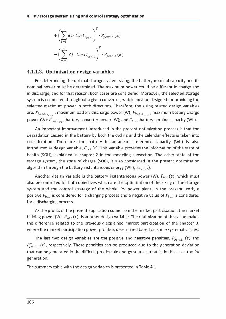
4. IPV storage system sizing and control strategy optimization
106
+
=1
+ + ( )
=1
( )
4.1.1.3. Optimization design variables
For determining the optimal storage system sizing, the battery nominal capacity and its
nominal power must be determined. The maximum power could be different in charge and
in discharge, and for that reason, both cases are considered. Moreover, the selected storage
system is connected throughout a given converter, which must be designed for providing the
selected maximum power in both directions. Therefore, the sizing related design variables
are: , maximum battery discharge power (W); , maximum battery charge
power (W); , battery converter power (W); and , battery nominal capacity (Wh).
An important improvement introduced in the present optimization process is that the
degradation caused in the battery by both the cycling and the calendar effects is taken into
consideration. Therefore, the battery instantaneous reference capacity (Wh) is also
introduced as design variable, ( ). This variable provides the information of the state of
health (SOH), explained in chapter 2 in the modeling subsection. The other state of the
storage system, the state of charge (SOC), is also considered in the present optimization
algorithm through the battery instantaneous energy (Wh), ( ).
Another design variable is the battery instantaneous power (W), ( ), which must
also be controlled for both objectives which are the optimization of the sizing of the storage
system and the control strategy of the whole IPV power plant. In the present work, a
positive is considered for a charging process and a negative value of is considered
for a discharging process.
As the profits of the present application come from the market participation, the market
bidding power (W), ( ), is another design variable. The optimization of this value makes
the difference related to the previously explained market participation of the chapter 3,
where the market participation power profile is determined based on some systematic rules.
The last two design variables are the positive and negative penalties, + ( ) and
( ), respectively. These penalties can be produced due to the generation deviation
that can be generated in the difficult predictable energy sources, that is, in this case, the PV
generation.
The summary table with the design variables is presented in Table 4.1.
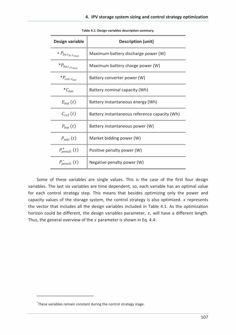
4. IPV storage system sizing and control strategy optimization
107
Table 4.1: Design variables description summary.
Design variable Description (unit)
Maximum battery discharge power (W)
* Maximum battery charge power (W)
* Battery converter power (W)
* Battery nominal capacity (Wh)
( ) Battery instantaneous energy (Wh)
( ) Battery instantaneous reference capacity (Wh)
( ) Battery instantaneous power (W)
( ) Market bidding power (W)
+ ( ) Positive penalty power (W)
( ) Negative penalty power (W)
Some of these variables are single values. This is the case of the first four design
variables. The last six variables are time dependent, so, each variable has an optimal value
for each control strategy step. This means that besides optimizing only the power and
capacity values of the storage system, the control strategy is also optimized. represents
the vector that includes all the design variables included in Table 4.1. As the optimization
horizon could be different, the design variables parameter, , will have a different length.
Thus, the general overview of the parameter is shown in Eq. 4.4:
*These variables remain constant during the control strategy stage.

4. IPV storage system sizing and control strategy optimization
108
=( ) × 1
( ) × 1
( ) × 1
( ) × 1
+ ( ) × 1
( ) × 1 (4+6 ) × 1
Eq. 4.4
As an example, for the case of a single day optimization with a ten minutes time step,
the size of the parameter length is calculated as follows.
= 2460
1
1
10 = 144
[4 + 6 144 × 1] = [868 × 1] Eq. 4.5
The lower and upper bounds of the design variables are also included in order to
represent a real scenario (the battery capacity can only be a positive value, or the energy
stored in the battery must be positive), but giving to the optimization the ability to fix the
maximum and minimum values. Therefore, the lower ( ) and upper ( ) bounds of the
variables are defined as in Eq. 4.6.
=
0
0
0
0 × 1
0 × 1
× 1
0 × 1
0 × 1
× 1
=
0
× 1
× 1
× 1
× 1
× 1
0 × 1
Eq. 4.6
4.1.1.4. Optimization constraints
The optimization constraints are related to several physical and economic aspects of the
whole IPV power plant and are listed below:
Battery exchange power
Battery associated converter power
Update of the state of charge, SOC
Update of the state of health, SOH
Battery ageing processes
Regulatory issues
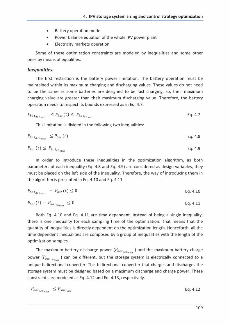
4. IPV storage system sizing and control strategy optimization
109
Battery operation mode
Power balance equation of the whole IPV power plant
Electricity markets operation
Some of these optimization constraints are modeled by inequalities and some other
ones by means of equalities.
Inequalities:
The first restriction is the battery power limitation. The battery operation must be
maintained within its maximum charging and discharging values. These values do not need
to be the same as some batteries are designed to be fast charging, so, their maximum
charging value are greater than their maximum discharging value. Therefore, the battery
operation needs to respect its bounds expressed as in Eq. 4.7.
( ) Eq. 4.7
This limitation is divided in the following two inequalities:
( ) Eq. 4.8
( ) Eq. 4.9
In order to introduce these inequalities in the optimization algorithm, as both
parameters of each inequality (Eq. 4.8 and Eq. 4.9) are considered as design variables, they
must be placed on the left side of the inequality. Therefore, the way of introducing them in
the algorithm is presented in Eq. 4.10 and Eq. 4.11.
( ) 0 Eq. 4.10
( ) 0 Eq. 4.11
Both Eq. 4.10 and Eq. 4.11 are time dependent. Instead of being a single inequality,
there is one inequality for each sampling time of the optimization. That means that the
quantity of inequalities is directly dependent on the optimization length. Henceforth, all the
time dependent inequalities are composed by a group of inequalities with the length of the
optimization samples.
The maximum battery discharge power ( ) and the maximum battery charge
power ( ) can be different, but the storage system is electrically connected to a
unique bidirectional converter. This bidirectional converter that charges and discharges the
storage system must be designed based on a maximum discharge and charge power. These
constraints are modeled as Eq. 4.12 and Eq. 4.13, respectively.
Eq. 4.12

4. IPV storage system sizing and control strategy optimization
110
Eq. 4.13
As in the previous case, as both parameters of each inequality (Eq. 4.12 and Eq. 4.13)
are design variables, they must be placed on the left side of the inequality. Therefore, the
way of introducing them in the algorithm is presented in Eq. 4.14 and Eq. 4.15.
0 Eq. 4.14
0 Eq. 4.15
Those inequalities are not time dependent.
Another group of constraints is related to the energy limitation of the storage system.
As in the case of the power limitation, the energy of the storage system must be maintained
within its limits as it has been presented in Eq. 4.16. This equation represents the
variation, but instead of working with percentage values, it is represented in energy values,
Wh.
( ) ( ) ( ) Eq. 4.16
Where and are the minimum and maximum state of charge of the
storage system, both of them in percentage. The other terms are the design variables that
have been already explained. This limitation is divided into two inequalities, as follows:
( ) ( ) Eq. 4.17
( ) ( ) Eq. 4.18
These inequalities represent the energy limitation downward, when the storage system
is fully discharged, and upward, when the storage system is fully charged. The way to
introduce them as optimization constraints is presented in Eq. 4.19 and Eq. 4.20.
( ) ( ) 0 Eq. 4.19
( ) ( ) 0 Eq. 4.20
Another inequality is related to the of the storage system. It considers the capacity
losses related to the battery nominal capacity. Therefore, Eq. 4.21 determines the end of life
(EOL) of the storage system, analyzing the battery instantaneous reference capacity, ( ).
This EOL is considered as percentage of the nominal capacity.
( ) Eq. 4.21
Where is the minimum state of health in percentage, the value where the EOL
of the storage system is considered. Below this value, the storage system can no longer be
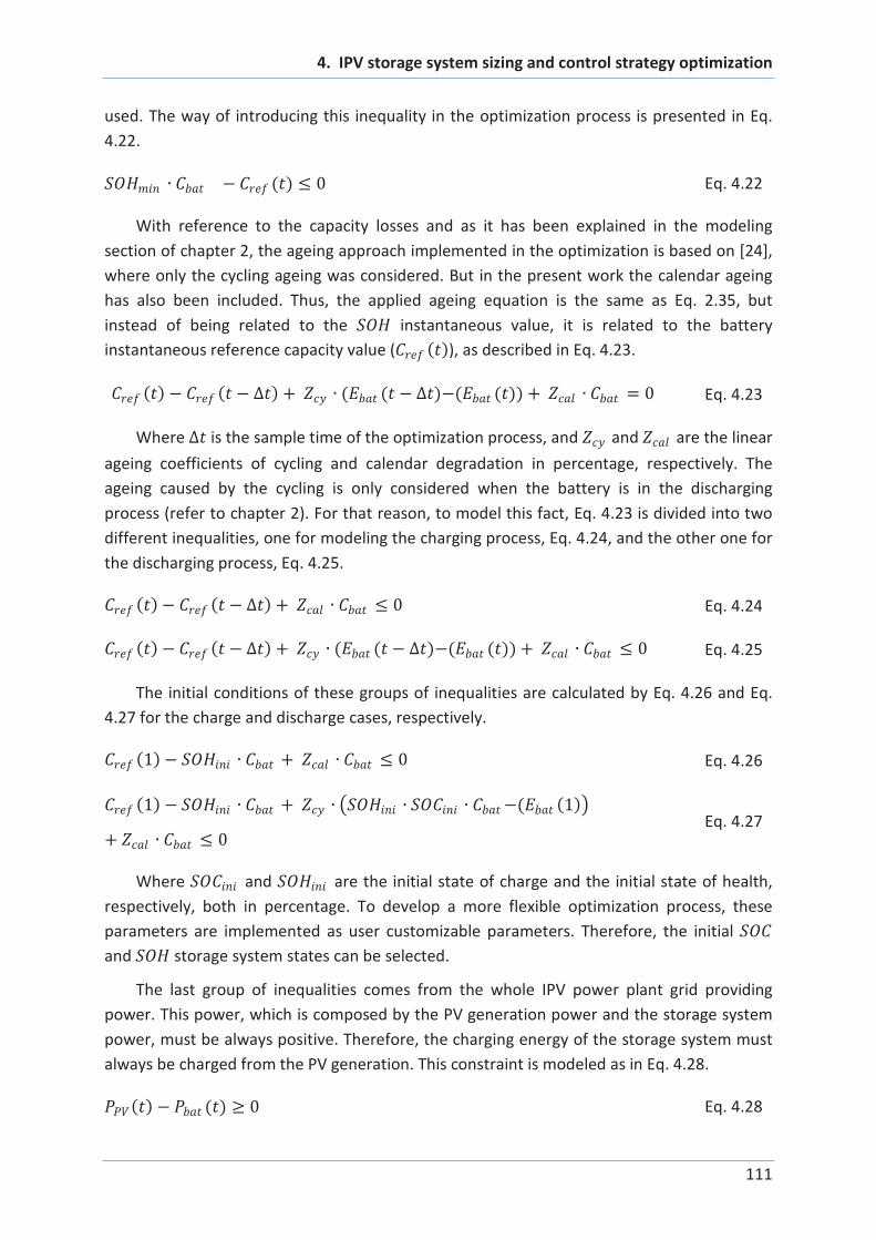
4. IPV storage system sizing and control strategy optimization
111
used. The way of introducing this inequality in the optimization process is presented in Eq.
4.22.
( ) 0 Eq. 4.22
With reference to the capacity losses and as it has been explained in the modeling
section of chapter 2, the ageing approach implemented in the optimization is based on [24],
where only the cycling ageing was considered. But in the present work the calendar ageing
has also been included. Thus, the applied ageing equation is the same as Eq. 2.35, but
instead of being related to the instantaneous value, it is related to the battery
instantaneous reference capacity value ( ( )), as described in Eq. 4.23.
( ) ( ) + ( ( ) ( ( )) + = 0 Eq. 4.23
Where is the sample time of the optimization process, and and are the linear
ageing coefficients of cycling and calendar degradation in percentage, respectively. The
ageing caused by the cycling is only considered when the battery is in the discharging
process (refer to chapter 2). For that reason, to model this fact, Eq. 4.23 is divided into two
different inequalities, one for modeling the charging process, Eq. 4.24, and the other one for
the discharging process, Eq. 4.25.
( ) ( ) + 0 Eq. 4.24
( ) ( ) + ( ( ) ( ( )) + 0 Eq. 4.25
The initial conditions of these groups of inequalities are calculated by Eq. 4.26 and Eq.
4.27 for the charge and discharge cases, respectively.
(1) + 0 Eq. 4.26
(1) + ( (1)
+ 0 Eq. 4.27
Where and are the initial state of charge and the initial state of health,
respectively, both in percentage. To develop a more flexible optimization process, these
parameters are implemented as user customizable parameters. Therefore, the initial
and storage system states can be selected.
The last group of inequalities comes from the whole IPV power plant grid providing
power. This power, which is composed by the PV generation power and the storage system
power, must be always positive. Therefore, the charging energy of the storage system must
always be charged from the PV generation. This constraint is modeled as in Eq. 4.28.
( ) ( ) 0 Eq. 4.28

4. IPV storage system sizing and control strategy optimization
112
Where ( ) (W) is the photovoltaic generation power profile. It is worth to remember
that a positive battery power is a charge process, and for that reason the battery power
profile is included as a negative term to model a battery discharge process, which implies an
energy flow from the battery to the grid. In order to introduce this constraint in the
optimization process, Eq. 4.28 is transformed into Eq. 4.29. As the ( ) is not a design
variable, neither a multiplier of some design variables, it must be located in the right side of
the inequality.
( ) ( ) Eq. 4.29
All the explained inequalities compose the matrix and vector of Eq. 4.37 and Eq.
4.38 respectively, which are included in the optimization as follows:
1st row: Inequality represented by Eq. 4.14 [1 X (4+6·length)].
2nd row: Inequality represented by Eq. 4.15 [1 X (4+6·length)].
3rd row: Group of inequalities represented by Eq. 4.10 [length X (4+6·length)].
4th row: Group of inequalities represented by Eq. 4.11 [length X (4+6·length)].
5th row: Group of inequalities represented by Eq. 4.19 [length X (4+6·length)].
6th row: Group of inequalities represented by Eq. 4.20 [length X (4+6·length)].
7th row: Group of inequalities represented by Eq. 4.22 [length X (4+6·length)].
8th row: Group of inequalities represented by Eq. 4.24 [length X (4+6·length)],
with the initial inequality Eq. 4.26.
9th row: Group of inequalities represented by Eq. 4.25 [length X (4+6·length)],
with the initial inequality Eq. 4.27.
10th row: Group of inequalities represented by Eq. 4.29 [length X
(4+6·length)].
Equalities:
The first equality represents the battery operation that models its energy flow. This
equation is the same as the Eq. 2.21 explained in chapter 2, but considering the energy of
the storage system, , instead of the . Moreover, to maintain the objective of
modeling a linear problem, the efficiency term ( ) is removed due to the fact that it includes
a non-linearity. Therefore, the efficiency is not considered in the purely optimization process
but it is taken into account in the following step. The equation that models this behavior is
shown in Eq. 4.30.
( ) = ( ) + ( ) Eq. 4.30
Once again, in order to introduce this equation in the optimization process, it is
transformed into the form presented in Eq. 4.31.
( ) ( ) ( ) = 0 Eq. 4.31
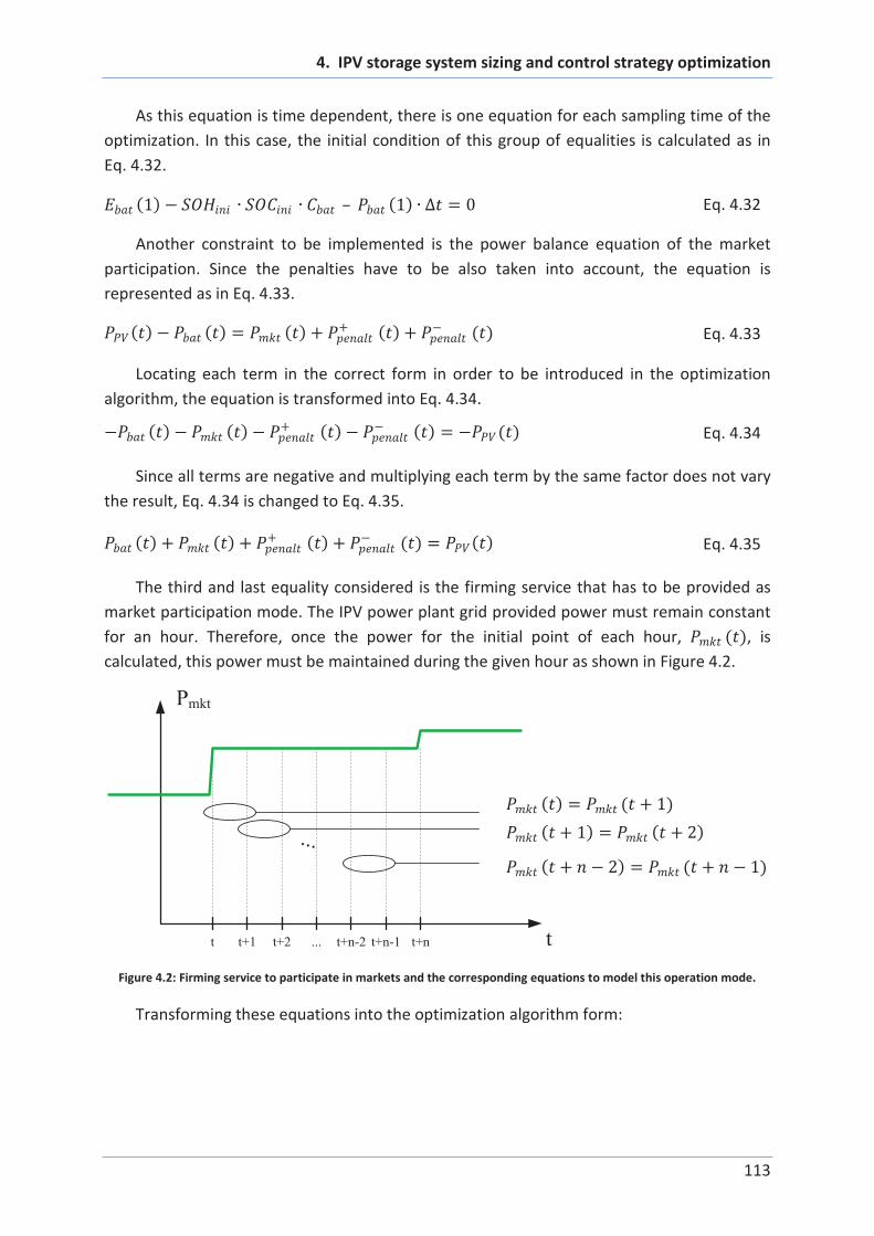
4. IPV storage system sizing and control strategy optimization
113
As this equation is time dependent, there is one equation for each sampling time of the
optimization. In this case, the initial condition of this group of equalities is calculated as in
Eq. 4.32.
(1) – (1) = 0 Eq. 4.32
Another constraint to be implemented is the power balance equation of the market
participation. Since the penalties have to be also taken into account, the equation is
represented as in Eq. 4.33.
( ) ( ) = ( ) + + ( ) + ( ) Eq. 4.33
Locating each term in the correct form in order to be introduced in the optimization
algorithm, the equation is transformed into Eq. 4.34.
( ) ( ) + ( ) ( ) = ( ) Eq. 4.34
Since all terms are negative and multiplying each term by the same factor does not vary
the result, Eq. 4.34 is changed to Eq. 4.35.
( ) + ( ) + + ( ) + ( ) = ( ) Eq. 4.35
The third and last equality considered is the firming service that has to be provided as
market participation mode. The IPV power plant grid provided power must remain constant
for an hour. Therefore, once the power for the initial point of each hour, ( ), is
calculated, this power must be maintained during the given hour as shown in Figure 4.2.
t
Pmkt
t t+1 t+2 ... t+n-2 t+n-1 t+n
...
Figure 4.2: Firming service to participate in markets and the corresponding equations to model this operation mode.
Transforming these equations into the optimization algorithm form:
( ) = ( + 1)
( + 1) = ( + 2)
( + 2) = ( + 1)

4. IPV storage system sizing and control strategy optimization
114
( ) ( + 1) = 0
( + 1) ( + 2) = 0
( + 2) ( + 1) = 0
Eq. 4.36
As it can be evaluated from Eq. 4.36, the number of needed equations for each hour is
1, considering as the number of equations needed for each hour depending on the
sample time. This special behavior is modelled by means of the auxiliary matrix ,
presented in Eq. 4.43.
All the exposed equalities compose the matrix and vector of Eq. 4.39 and Eq.
4.40 respectively, which are included in the optimization as follows:
1st row: Group of equalities represented by Eq. 4.31 [length X (4+6·length)],
with the initial equality Eq. 4.32.
2nd row: Group of equalities represented by Eq. 4.35 [length X (4+6·length)].
3rd row: Group of inequalities represented by Eq. 4.36 [length X (4+6·length)].
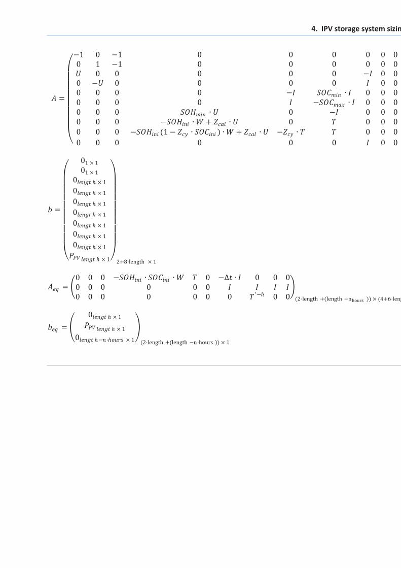
4. IPV storage system sizing and control strategy optimizat
=
1 0 1 0 0 0 0 0 0 0
0 1 1 0 0 0 0 0 0 0
0 0 0 0 0 0 0 0
0 0 0 0 0 0 0 0
0 0 0 0 0 0 0 0
0 0 0 0 0 0 0 0
0 0 0 0 0 0 0 0
0 0 0 + 0 0 0 0 0
0 0 0 (1 ) + 0 0 0 0
0 0 0 0 0 0 0 0 0 (
=
01 × 1
01 × 1
0 × 1
0 × 1
0 × 1
0 × 1
0 × 1
0 × 1
0 × 1
× 1 2+8·length × 1
=0 0 0 0 0 0 0
0 0 0 0 0 0
0 0 0 0 0 0 0 0 0 (2·length +(length nhours )) × (4+6·length )
=
0 × 1
× 1
0 · × 1 (2·length +(length n·hours )) × 1

4. IPV storage system sizing and control strategy optimization
116
= 1
length × 1
, = 1
1 length × 1
, =
1
0
0 length × 1
, =1 0 0
0 0
0 0 1 length × length
=
1 0 0
1 1
0 1
1 1 0
0 0 1 1 length × length
, =
1 1 0 0
0 1 1
1 1 0
0 0 1 1 length hour 1 × length hour
=
0 0
0
0
0 0 length nhours × length
The vectors and matrixes presented in Eq. 4.41, Eq. 4.42 and Eq. 4.43 are some sub matrixes or auxiliary matrixes included in matrixes
and and vectors and for an easier visualization:
The single column matrix includes the PV power generation values for each sample time of the given optimization
The matrix is a single column auxiliary matrix composed by ones.
The matrix is a single column auxiliary matrix composed by one being the first value and all the other values are zero.
The matrix is the identity matrix.
The matrix is an auxiliary square matrix, which has the main diagonal composed by ones and the lower bidiagonal composed by
minus ones. This matrix is used to represent a subtraction of a given value with its previous one, as in
The matrix is an auxiliary matrix composed by the matrix without its first row. As it is mentioned before, it is used t
the firming service that has to be provided for participating in electricity markets. This matrix models a one hour operation
The matrix is an auxiliary matrix composed by several matrixes in the main diagonal to complete the
optimization. For each hour in the developed optimization, a column that includes another matrix is needed.

4. IPV storage system sizing and control strategy optimization
117
4.1.1.5. Algorithm selection and application
Once the objective function, the design variables and all the constraints have been
described, the optimization algorithm selection and application is carried out. As it has been
verified, all equations that model the objective function and the constraints are included as
linear equations. Thus, the objective of using a linear programming (LP) optimization process
is achieved.
The LP optimization algorithm is executed in Matlab by the function (included
in the Optimization Toolbox [154]). Therefore, Eq. 4.1 can be rewritten as Eq. 4.44.
Where is the vector composed by the design variables; ( ) is the linear objective
function; is the transposed vector composed by the multipliers of (for that reason is a
linear programming problem); and are the constraints matrixes; and are the
constraints vectors; and and are the vectors of lower and upper bounds of the design
variables.
The LP optimization in Matlab comes with several solvers as the interior-point, the
simplex, the dual-simplex, and the active-set [154, 155]. Each of them follows a different
iterative process to search the optimal solution. In the present case, the interior-point is
used as it is the one recommended for large scale optimization processes.
4.1.1.6. Simulation execution process
With the previous algorithm application the co-optimization process is almost complete
but there is an input/output correlation that is solved within the process proposed in the
present subsection.
Based on this optimization, the sizing and optimal operation values can be obtained
almost simultaneously. Nevertheless, one of the inputs of the objective function is the
lifetime of the battery ( ) which is calculated based on the Rainflow cycling counting
algorithm and the depth of discharge data of both the battery manufacturer and the
different cycling tests carried out in the energy storage laboratory of Ikerlan. Therefore, one
of the outputs of the optimization (the battery power profile) has an influence on one of the
inputs (the lifetime of the battery). In order to solve this modeling constraint, an iterative
execution of the optimization must be carried out, aiming to obtain the optimal values based
on the real lifetime of the battery. Thus, the proposed simulation follows the diagram of
Figure 4.3.
( ) =
,
= ,
.
Eq. 4.44

4. IPV storage system sizing and control strategy optimization
118
?
| ( 1) ( )| >
| ( 1) ( )| >
| ( 1) ( )| >
Initialization
Pre-simulation
Optimization
Post-processing Update variables
yes
noi
Results treatment
End
i++
<
<
<
Figure 4.3: Complete simulation execution flowchart.
In the initialization step, all the parameters are initialized by means of defining the size
of the simulation process. In the pre-simulation step, an initial lifetime of the battery is
calculated to run the following optimization step. The optimization step executes the
optimization process described in the previous sections. In the post-processing step the
optimization results are processed in order to verify if the next condition is fulfilled. If the
results regarding the battery capacity ( ), the objective function ( ) and the lifetime of
the battery ( ) are maintained within their respective error thresholds ( , and
, respectively) between the previous optimization iteration ( 1) and the last iteration
( ), the results are processed (results treatment) and the optimization algorithm is finished. If
not, the Rainflow algorithm is executed in the update variables step for running the next
optimization iteration. The error thresholds ( , and ) have been selected
around the 1% of each parameter final result after several trial and error repetitions.
Once the co-optimization process has been explained, the next sections focus on the
proposed process to get the optimal sizing and the optimal operation of the IPV power plant.
This process is separated into two stages, which are the Design Stage and the Operation
Stage. On the first one, the optimal sizing of the storage system is determined and on the
second one the optimal control strategy to participate in electricity markets is established.
Both stages of this process are detailed hereafter.
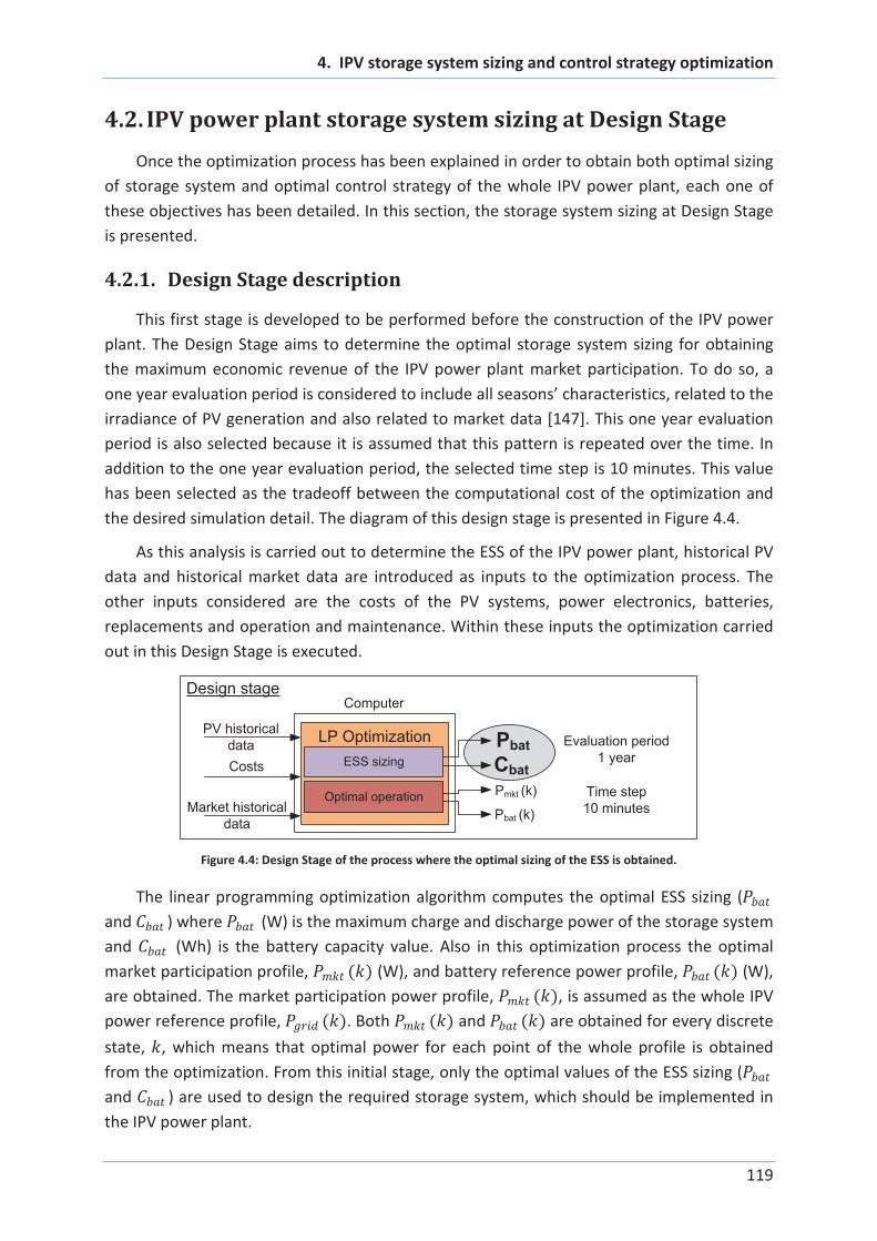
4. IPV storage system sizing and control strategy optimization
119
4.2. IPV power plant storage system sizing at Design Stage
Once the optimization process has been explained in order to obtain both optimal sizing
of storage system and optimal control strategy of the whole IPV power plant, each one of
these objectives has been detailed. In this section, the storage system sizing at Design Stage
is presented.
4.2.1. Design Stage description
This first stage is developed to be performed before the construction of the IPV power
plant. The Design Stage aims to determine the optimal storage system sizing for obtaining
the maximum economic revenue of the IPV power plant market participation. To do so, a
one year evaluation period is considered to include all seasons’ characteristics, related to the
irradiance of PV generation and also related to market data [147]. This one year evaluation
period is also selected because it is assumed that this pattern is repeated over the time. In
addition to the one year evaluation period, the selected time step is 10 minutes. This value
has been selected as the tradeoff between the computational cost of the optimization and
the desired simulation detail. The diagram of this design stage is presented in Figure 4.4.
As this analysis is carried out to determine the ESS of the IPV power plant, historical PV
data and historical market data are introduced as inputs to the optimization process. The
other inputs considered are the costs of the PV systems, power electronics, batteries,
replacements and operation and maintenance. Within these inputs the optimization carried
out in this Design Stage is executed.
LP Optimization
ESS sizing
Optimal operation
Costs
Market historical
data
Pbat
Cbat
Design stage
Pmkt (k)
Pbat (k)
Evaluation period
1 year
Time step
10 minutes
Computer
PV historical
data
Figure 4.4: Design Stage of the process where the optimal sizing of the ESS is obtained.
The linear programming optimization algorithm computes the optimal ESS sizing (
and ) where (W) is the maximum charge and discharge power of the storage system
and (Wh) is the battery capacity value. Also in this optimization process the optimal
market participation profile, ( ) (W), and battery reference power profile, ( ) (W),
are obtained. The market participation power profile, ( ), is assumed as the whole IPV
power reference profile, ( ). Both ( ) and ( ) are obtained for every discrete
state, , which means that optimal power for each point of the whole profile is obtained
from the optimization. From this initial stage, only the optimal values of the ESS sizing (
and ) are used to design the required storage system, which should be implemented in
the IPV power plant.

4. IPV storage system sizing and control strategy optimization
120
The other variables included in the before explained design variables parameter ( ) are
used to verify the correct execution of the optimization and the operation of the storage
system.
The evaluation of a whole year requires a large optimization size which cannot be
carried out by the solver proposed by the Matlab software. As the selected time step is 10
minutes, the length of the parameter and of the matrix of the whole year optimization
are calculated as follows:
= 36524
1
60
1
1
10 = 52560
[4 + 6 52560 × 1] = [315364 × 1]
[(2 + 8 · length) × (4 + 6 · length)] = [420482 × 315364]
Eq. 4.45
The class of a standard Matlab variable is double, which means that it is composed by 8
bytes (B) or 64 bits (b). For that reason, the memory allocation of each variable is 8 bytes.
Analyzing the 315364 variables of the parameter, its memory allocation is calculated as:
315364 8 = 2522912 ~ 2463 ~ 2.4 Eq. 4.46
The same process is carried out to calculate the memory allocation of the matrix :
(420482 315364) 8 = 1.061 1012 ~ 988G Eq. 4.47
With these sizes (and memory allocations), it is verified that the optimization terms are
large enough to be infeasible by the Matlab software in regular conditions. The simulations
of this optimal sizing step are implemented on an Intel Core i5 CPU 3.1GHz with 16 GB of
RAM. For that reason, it has been decided to reduce the optimization length to a single
month. In this way the lengths of the vector and matrix are reduced to the following values
(for a 31 day month).
= 3124
1
60
1
1
10 = 4464
[4 + 6 4464 × 1] = [26788 × 1]~209
[(2 + 8 · length) × (4 + 6 · length)] = [35714 × 26788] ~ 7.12
Eq. 4.48
Although the resulting sizes are still large, the Matlab software and the used computer
are able to work with them. Therefore, in order to take into account the whole year, the 12
month optimizations are carried out separately. The flowchart applied to represent this
optimization execution is presented in Figure 4.5. It is the same as the one explained in the
optimization execution process section (4.1.1.6) with an additional loop that evaluates the
12 months and an additional block to save each month’s results.

4. IPV storage system sizing and control strategy optimization
121
In the last block named as Results treatment, a statistic analysis of the results of this
optimization process is applied in order to determine the optimal size for the battery. This
process is analyzed in the next results’ section.
?
| ( 1) ( )| >
| ( 1) ( )| >
| ( 1) ( )| >
Initialization
Pre-simulation
Optimization
Post-processing Update variables
no
yesi
Results treatment
End
i++
Save results
months<12? yesi
month++
no
Figure 4.5: Design Stage of the process where the optimal sizing is determined.
4.2.2. Optimal storage system sizing results
In this section the results related to the optimal sizing obtained in the Design Stage are
presented. The optimization is applied for the case study presented in chapter 2. In the next
table, the main characteristics of this IPV power plant are summarized.
Table 4.2: IPV power plant main characteristics.
Parameter description Value
Installed PV power 1 MW / 1.2 MWp
Battery inverter maximum power 1 MW
Battery nominal capacity 560 kWh

4. IPV storage system sizing and control strategy optimization
122
As it has been mentioned before, a whole year optimization is carried out but based on
monthly size optimizations. With a time step of 10 minutes, efficient and computationally
light monthly length optimizations are carried out obtaining, for each month, the optimal
and values. As each month has a different length, the size of each month
optimization matrix is different. The size of matrix is [34562 x 25924] for a 30 days month;
[35714 x 26788] for a 31 days month; and [32258 x 24196] for the 28 days of February. The
PV predictions taken into account are the real generation data presented in Figure 2.9, in
chapter 2, section 2.3.1. Therefore, perfect predictions are considered for this sizing
optimization because the objective is to firm the PV generation profile to participate in
electricity markets in the optimal operation mode. There will be PV deviations, but in both
directions, so it is assumed an error with a null mean value, and thus, the positive deviations
are counteracted in a natural way with the negative ones.
The results obtained for each month are summarized in the next figures. In Figure 4.6
each month battery power capacity value ( ) is presented, with the mean value
represented by the red horizontal line. In Figure 4.7, the energetic capacity values are
presented ( ) with the maximum and minimum values highlighted together with the
mean and barycenter values. In Figure 4.8, the calculated life span of each optimization is
shown also with the average value highlighted. In Figure 4.9, each month benefits of the
whole IPV power plant (PV + BESS) are depicted; and finally, in Figure 4.10, the relation
between the capacity value and the benefits is shown, together with the calculated
barycenter. This value is calculated weighting each month capacity value with the benefits of
the own month optimization.
Figure 4.6: Design stage ESS sizing optimization results: battery power capacity values.
The results related to the storage system power needs show a similar optimal value for
the whole year. This value, 511kW, is the half of the installed PV power (1 MW), and the half
of the installed converter in the case study IPV power plant. This result provides useful
information regarding the relation between the PV power and the storage system power
needs. The mean value is taken into account as the optimal one, because when the worst
1 2 3 4 5 6 7 8 9 10 11 120
1
2
3
4
5
6
x 105 Battery power capacities
Time [months]
Pow
er
[W]
Battery power capacity

4. IPV storage system sizing and control strategy optimization
123
case is considered the system is oversized the most part of the time (which is not the
objective: indeed, it results in a sub-optimal economic optimization). It means that in that
case, the ESS power capabilities will not be able to fully compensate the needed
requirement, but from the global (economic) point of view, this is the optimal scenario.
Figure 4.7: Design stage ESS sizing optimization results: battery energy capacity values.
With reference to the capacity value, the difference among the months is much more
representative, obtaining almost a factor two between the optimal values of May and April,
compared to July and December. Nevertheless, several months’ optimal values are similar
and are around the average value of 426kWh. In the capacity analysis case, the barycenter is
calculated, analyzing each month capacity value related to its benefits. The result of the
barycenter is also very similar: 433kWh. As the difference between them is lower than 2%,
the optimal value selected is the one obtained using the barycenter (433kWh). This value is
more representative because it includes the value of the benefits for each month. This result
provides a significant reduction (around 23 %) comparing to the installed storage capacity of
the presented case study, which is 560 kWh. As it has been mentioned before, with this
capacity the worst case is not fulfilled, but from the global (economic) point of view, it is
better than the worst case, which oversizes again the storage system. The objective is not to
fulfill all cases but to obtain the optimal storage system.
1 2 3 4 5 6 7 8 9 10 11 120
1
2
3
4
5
6
7x 10
5 Battery energy capacities
Time [months]
Capacity [
Wh]
Battery energetic capacity
Mean value
Barycenter value
Max value
Min value

4. IPV storage system sizing and control strategy optimization
124
Figure 4.8: Design stage ESS sizing optimization results: battery life span values.
The life span results of the present optimization vary between 7 and 9 years of lifetime.
In summer months, the life span is reduced, which could be caused by the greater use of the
ESS in this period of time. Nevertheless, the results are close to the average value of 8 years,
which enforces the resultant average value.
Figure 4.9: Design stage ESS sizing optimization results: obtained benefits values.
The results of the obtained benefits present an inverse effect compared with the
previous lifetime results. As in summer there are sunnier days and more hours of sun per
day, the obtained benefits increase in the same proportion.
The obtained annual benefit is around 65000€. Although it seems low, the yearly
average PV generation in this location is around 1300MWh at an average daily market price
of 42 €/MWh. Therefore, the optimization increases the profits from 54600€ to 65000€
(around 20%). Of course, this economic difference justifies the decision of including the
energy storage system.
1 2 3 4 5 6 7 8 9 10 11 120
1
2
3
4
5
6
7
8
9
Life span of the battery
Time [months]
Life s
pan [
years
]
1 2 3 4 5 6 7 8 9 10 11 120
1000
2000
3000
4000
5000
6000
7000
8000
9000Obtained benefits based on optimal algorithm
Time [months]
Benefits
[€]
Optimal benefits
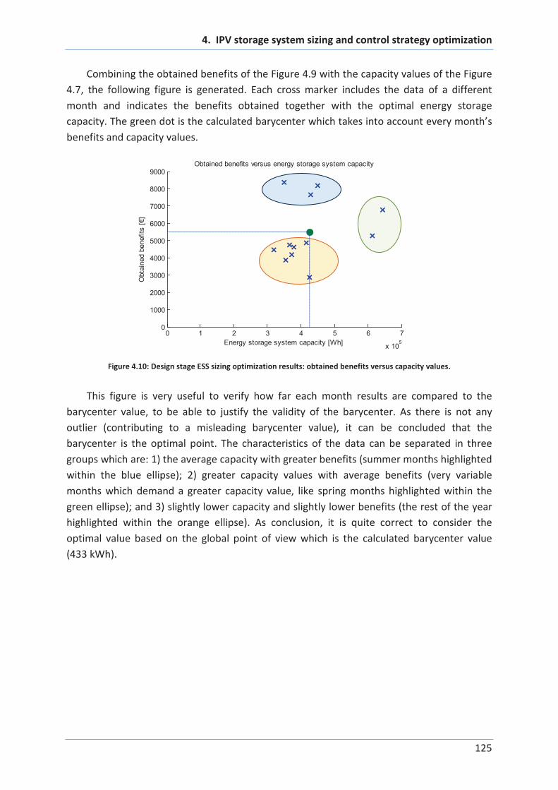
4. IPV storage system sizing and control strategy optimization
125
Combining the obtained benefits of the Figure 4.9 with the capacity values of the Figure
4.7, the following figure is generated. Each cross marker includes the data of a different
month and indicates the benefits obtained together with the optimal energy storage
capacity. The green dot is the calculated barycenter which takes into account every month’s
benefits and capacity values.
Figure 4.10: Design stage ESS sizing optimization results: obtained benefits versus capacity values.
This figure is very useful to verify how far each month results are compared to the
barycenter value, to be able to justify the validity of the barycenter. As there is not any
outlier (contributing to a misleading barycenter value), it can be concluded that the
barycenter is the optimal point. The characteristics of the data can be separated in three
groups which are: 1) the average capacity with greater benefits (summer months highlighted
within the blue ellipse); 2) greater capacity values with average benefits (very variable
months which demand a greater capacity value, like spring months highlighted within the
green ellipse); and 3) slightly lower capacity and slightly lower benefits (the rest of the year
highlighted within the orange ellipse). As conclusion, it is quite correct to consider the
optimal value based on the global point of view which is the calculated barycenter value
(433 kWh).
0 1 2 3 4 5 6 7
x 105
0
1000
2000
3000
4000
5000
6000
7000
8000
9000Obtained benefits versus energy storage system capacity
Energy storage system capacity [Wh]
Obta
ined b
enefits
[€]

4. IPV storage system sizing and control strategy optimization
126
4.3. IPV power plant control strategy at Operation Stage
Once the optimal storage system has been obtained, in this Operation Stage, the IPV
power plant control strategy is optimized, to participate in electricity markets. This section
includes the control strategy definition to participate in electricity markets, and the market
participation based on MPC with this optimal strategy.
4.3.1. Control strategy definition
The Operation Stage of the proposed process includes two steps related to the two
electricity markets that the IPV power plant participates on. The optimization applied in both
steps considers a fixed storage system size, which is the output of the previous explained
design stage. The first step is the generation planning for participating in the daily market of
the following day. The second step is the online operation, where the PV generation
prediction errors are counteracted participating in the intraday markets. This second step is
carried out thanks to the MPC in order to be able to participate in the different intraday
markets to recover the benefits that the PV prediction errors have been generated. That is
why the MPC is implemented and is necessary to be able to have the possibility to
participate in the intraday markets in order to improve the economic revenues of the IPV
power plant. The operation stage block diagram is presented in Figure 4.11. It is similar to
the one explained in chapter 3 but including the optimal control strategy.
Regarding the market participation, instead of the power value calculated by the
optimization process, ( ), a detailed market participation offer is composed by an
energy offer, ( ), at a given cost, ( ), for each hour. As in this operation
stage the market participation is the core idea, these parameters are used to explain in
detail the whole operation.

4. IPV storage system sizing and control strategy optimization
127
*
Plant controller
Generation planning
PV forecast
(1:24)
Market forecastEoffered(k)
MPC
PV forecast
(k:24)
Ecleared(k)
Eoffered(k)
Ecleared(k)
Pbat(k)
Pbat meas (k)SOC(k)
PPV meas (k)
Tim
e s
equence
DC
AC
PV
PV local controller
Battery localcontroller
BMS
DC
AC
Battery
IPV plant Grid
PCC
comms
Plantcontroller
Pgrid(k)
Online operation
Market
Daily market
Pgrid(k)
*
IMj
DM
DM
IMj
IMj)))))))))
Intraday markets
...1
26
coffered(k)DM
ccleared(k)DM
1/hourEcleared(k)
ccleared(k)
coffered(k)IMj
ccleared(k)
LP Optimization
ESS fixed
Optimal operation
LP Optimization
ESS fixed
Optimal operation
Market forecast
Figure 4.11: Operation Stage block diagram, including the generation planning (to the daily market) and the online
operation step (to the intraday market).
The generation planning step is similar to the previously explained Design Stage. In this
case, the ESS rate is fixed and the relevant output of the applied optimization is the
generation planning offers to the daily market (DM) of the following day, ( ), at a
given cost, ( ), for each hour. This planning step is carried out the day before the
real operation. In order to make sure that the proposed offer is cleared, the offered hourly
cost must be zero or close to zero. Therefore, it is assumed that the offers sent to the market
operator are always cleared. The resolution of the DM is composed by the cleared energy,
( ), and the market clearing price, ( ), for each hour. This information is
obtained the day before the online operation and it is transformed into the initial power
reference profile, ( ) (W), to the online operation, which is the second step. This
explanation can be followed in the upper dotted blue rectangle of the Figure 4.11. A
flowchart to explain more in detail the market participation sequence of Figure 4.11 is
presented in Figure 4.12.

4. IPV storage system sizing and control strategy optimization
128
Run
optimization
Start
Send daily market
offer to MO
Receive cleared
market references
j=1
Calculate intraday
market j offer
Calculate grid
references
Send intraday market
j offer to MO
Receive cleared
market references
j++
Run
optimization
day d end?
End
No
Yes
Update grid
references
coffered(k)DM
Eoffered(k)DM
Ecleared(k)DM
ccleared(k)DM
Pgrid(k)*
ccleared(k)IMj
Ecleared(k)IMj
coffered(k)IMj
Eoffered(k)IMj
Update PV prediction
Pgrid(k)*
Online operation
Generation planning
k=ksend?IMjNo
Yes
k=kreceive?No
Yes
k++
IMj
From
optimization
results
MPC start
PPV(k)^
Pmkt(k)
Pbat(k)
Pmkt(k)
Pbat(k)
?
| ( 1) ( )| >
| ( 1) ( )| >
| ( 1) ( )| >
Initialization
Pre-simulation
Optimization
Post-processing Update variables
no
yesi
Results treatment
End
i++
?
| ( 1) ( )| >
| ( 1) ( )| >
| ( 1) ( )| >
Initialization
Pre-simulation
Optimization
Post-processing Update variables
no
yesi
Results treatment
End
i++
Figure 4.12: Detailed flowchart of the optimal strategy to participate in electricity markets.

4. IPV storage system sizing and control strategy optimization
129
The objective of the second step, the online operation step, is the operation of the IPV
power plant to maximize the economic revenues. This operation is managed using the
Model Predictive Control (MPC) [150, 151]. The inputs of this control are: the market cleared
power reference, ( ); PV generation forecast, ( . .24) (W); market prices
forecast; PV real power generation, ( ) (W); battery power, ( ) (W); and
the state of charge of the storage system, ( ) (%). The control outputs are the intraday
market’s (IM) offers (also an amount of energy for each hour, ( ), at a given cost,
( )) and the storage system reference power, ( ).
The internal process is detailed in the diagram of Figure 4.12, where it can be shown
that in the first step (generation planning), the output of the optimization related to the
battery profile is not used (and crossed out in the diagram), as the objective is to participate
in the daily market but the operation has not started yet. It is worth mentioning that the
block called Run optimization computes all the before explained process of Figure 4.3.
In the second step (online operation), the IPV power plant output power, ( ), must
be controlled every discrete state. Thereby, the optimal storage system reference power,
( ), is calculated every discrete state to maintain the IPV plant output power matching
the market cleared value, as it is stated in Eq. 4.49.
( ) = ( ) = ( ( )) Eq. 4.49
Moreover, the optimal market participation power profile ( ( )) is calculated every
discrete state, in the same optimization where the storage system power reference
( ( )) is calculated. Nevertheless, as there is no intraday market every discrete state, the
intraday market participation offer (an amount of energy for each hour, ( ), at a
given cost, ( )) is only calculated at the last discrete state before closing each
intraday market session ( ). There is an intraday market every 4 hours. The resolution
of the intraday markets is also composed by the intraday market session ( ) cleared
energy, ( ), and the market clearing price, ( ) for each hour. This resolution
is received at the discrete state , and added to the previously resolved markets to
update the power references for the IPV power plant, ( ).
The internal steps of the MPC operation have already been detailed in section 3.2.1 of
chapter 3 and therefore are not completely explained in this section. Even so and as a
summary, at each discrete state, the MPC optimizes the operation of a given window
(prediction horizon) based on the predictions and measures of some parameters, calculating
the optimal trajectory and the control input ( ( )) for obtaining this optimal trajectory
during the whole window. Nevertheless, only the first point of this control input ( 0( )) is
applied to the system. At the next discrete state, the operation is repeated, shifting the
window but maintaining its length. The optimization executed to calculate the control input
is the optimization proposed and explained in the present chapter.

4. IPV storage system sizing and control strategy optimization
130
Thus, the MPC runs the optimization every discrete state to obtain the optimal storage
system power ( ( )) and the optimal market participation power profile ( ( )).
Nevertheless, the market participation offer ( ( ) and ( )) is sent to the
market operator (MO) at the last discrete state where each intraday market session is
opened, at .
These MPC references are applied to the IPV power plant model, where the PV and ESS
models are included. As it has been mentioned before, the LP optimization does not take
into account the efficiency of the storage system (to be a linear programming optimization).
But in the model of the IPV power plant, where the MPC applies its calculated references,
this efficiency term ( ) is included. The efficiency of the storage system is directly
proportional to the charging power and inversely proportional to the discharging power.
Therefore, the equations that model this system are Eq. 4.50 and Eq. 4.51, respectively.
( ) = ( ) + ( ) Eq. 4.50
( ) ( ) ( )
= 0 Eq. 4.51
The introduction of this detailed model of the battery comprises a SOC reduction (or a
SOC increase) because when the controller requires a given power value to the storage
system (a discharge), in order to provide this amount at the output, a higher value is
extracted from the battery. This causes a higher SOC reduction than the expected one by
means of the optimization process. For that reason, the SOC is recalculated once the
efficiency of the battery is applied, to include the detailed SOC value to the next MPC
optimization step, as it can be shown in Figure 4.11.
4.3.2. Market participation based on MPC with optimal strategy
In this section the IPV power plant market participation analysis is presented. This
market participation analysis is executed considering the optimal 433 kWh storage system.
The analysis of the results of the market participation is based on a four day simulation,
as presented in Figure 4.13. It is the same example as the one used in chapter 3, presented
in Figure 3.11. As it can be observed, the presented simulation is oriented to explain the
second day (day ) market participation. For doing so, the simulation must start the first day
(day 1) in order to participate in the daily market. Therefore, once the daily market offer
has been sent (before midday of day 1), the MPC starts its operation. From this point, to
include the 24 hours of operation horizon of the day , 36 hours of MPC horizon is needed.
This horizon is also required due to the fact that the intraday session S1 has 27 hours of
length plus the period of time up to market session closing (more than 29 hours). The MPC
prediction horizon is depicted in the sliding red rectangles of Figure 4.13. The selected
sample time is 10 minutes. This value has been selected as the tradeoff between
computational cost of the optimization and the desired simulation detail.

4. IPV storage system sizing and control strategy optimization
131
00 04 08 12 16 20 00
Intraday 2
Intraday 3
Intraday 4
Intraday 5
Planing d+1
Intraday 6
Daily market
12
Intraday 1
Intraday 1
Daily marketPlaning d
12
16
20
04
08
00
16
20
00
12
04
08
16
20
04
08
00
00 04 08 12 16 20 00 04 08 12 16 20 00 04 08 12 16 200
Pow
er
[kW
]
day d-1 day d day d+1
Daily market
Intraday 1
MPC prediction
horizon
Intraday 2
Intraday 3
Intraday 4
Intraday 5
Intraday 6
Daily market
Intraday 1
00
12
04
08
16
20
00
Intraday market session open
Daily market session open
Daily market operation hours
Intraday market operation hours
day d+2
PV prediction
PV real generation
200
400
600
800
1000
MPC prediction horizon
Figure 4.13: Market participation example of the second day (day d) with the different markets operation hours,
participation periods and MPC prediction horizon.
At each sample time of 10 minutes, the MPC calculates the optimal battery exchanged
power ( ( )), considering the PV generation to maintain the market cleared power, which
is the IPV plant power reference profile ( ( )). Just before closing the intraday 1 market
session (blue square in Figure 4.13), the MPC calculates this market offer (when = 1 ),
based on the last PV predictions, PV measurements and battery SOC. This process is
repeated at each intraday session, knowing that each intraday operation horizon is different.
As the intraday markets are solved closer to their operation starting time, the PV prediction
could change and the participation on these markets permits to face the prediction changes
from their operation starting time. The operation is finished when the starting point of the
MPC prediction horizon crosses the end of the day d.
The simulations of this market participation are also implemented in MATLAB. The
presented optimization has been performed through the Optimization Toolbox [155]. The
whole simulation of a single day market operation is completed in around 15 minutes.
Some results of the explained market participation are presented in Figure 4.14, where
the simulation of two days market participation is carried out. The simulated days are
identical to the ones explained in chapter 3. The first day is detailed in Figure 4.14 a, b and c,
and is the day presented in Figure 4.13, which represents a sunny day. The second one is
detailed in Figure 4.14 d, e and f and is the day + 1 presented in Figure 4.13, which is a
cloudy day. Figure 4.14 depicts the market participation carried out in all the analyzed
markets, which are the daily and the six intraday markets. Figure 4.14 a and d show the PV
real generation and the PV predictions calculated by Eq. 3.11 and Eq. 3.12 as explained in
Chapter 3. Figure 4.14 b and e include the optimal market participation profile calculated to

4. IPV storage system sizing and control strategy optimization
132
participate in every market, based on the PV prediction, the measured PV generation and
the SOC of the storage system. Figure 4.14 c and f depict the six intraday markets’ offers. The
vertical grey lines included in Figure 4.14 b, c, e and f are the moments where the different
intraday market sessions offers are sent, .
Figure 4.14: Online operation results.
The seasonal effect of the PV prediction (calculated in Eq. 3.11) is presented by the black
profile of Figure 4.14 a and Figure 4.14 d. This profile is applied to determine the daily
market participation offer. In the MPC operation, where the intraday markets are resolved,
16 20 00 04 08 12 16 20 00 040
200
400
600
800
Time [h]
Pow
er
[kW
]
PV generation prediction and real generation profiles
16 20 00 04 08 12 16 20 00 040
200
400
600
800
Time [h]
Pow
er
[kW
]16 20 00 04 08 12 16 20 00 04
0
200
400
600
800
Time [h]
Pow
er
[kW
]
16 20 00 04 08 12 16 20 00 040
200
400
600
800Optimal market profiles calculated after every market session
Time [h]
Pow
er
[kW
]
16 20 00 04 08 12 16 20 00 04
-100
0
100
200
Generated intraday sessions market offer profiles
Time [h]
Pow
er
[kW
]
PV real generation PV pred daily PV pred MPC
DM IM1 IM2 IM3 IM4 IM5 IM6
IM1..6 sending time
16 20 00 04 08 12 16 20 00 04
-100
0
100
200
Time [h]
Pow
er
[kW
]
IM1..6 sending time
IM1 offer IM2 offer IM3 offer IM4 offer IM5 offer IM6 offer
(a) (d)
(b) (e)
(c) (f)

4. IPV storage system sizing and control strategy optimization
133
the PV prediction is calculated as in Eq. 3.12 and shown in the green profile. This profile is
closer to the real PV generation, and with this prediction the intraday markets could improve
the daily market cleared generation, maximizing the economic revenues.
Regarding Figure 4.14 b and e, the profiles included are the ones calculated by the
optimization of the MPC as optimal market profiles and the daily market offer. As it has been
mentioned before, the MPC takes into account the PV prediction, the PV measurement, the
SOC and the prices forecast. For that reason, an important power offer appears in all
markets in the hour 22 (from 21:00 to 22:00). This is because this hour is the most expensive
period in the Iberian Peninsula electricity market. This statement can be verified in Figure
2.15, on the second chapter. Therefore, the MPC decides to sell the overproduction stored in
the storage system in this hour.
After the daily market, the intraday S1 is resolved, and as this market can participate in
the last 3 hours of the previous day (it can be verified in Figure 4.13), the controller sells the
stored energy in the most expensive hour, once again the hour 22 (the first hour of the
intraday S1). This event can be shown by the blue profile in Figure 4.14 b and c for the sunny
day, and in the Figure 4.14 e and f for the cloudy day. In this intraday market, as it counts
with closer and better PV predictions, its market offer is the greatest one of all intraday
markets (around 200 kW during the sunny hours of the day).
As the PV prediction has not changed and there is no difference between the generation
estimation and the real generation during the night, the S2, S3 and S4 intraday sessions’
offers are almost zero, because it has already been cleared in previous markets (daily and
intraday session S1).
Until the discrete state where the intraday S5 is sent, there is little PV deviation from
the prediction to the real measurement, and for that reason, there is a little program change
in some hours (as it can be shown by the light blue profile of Figure 4.14 c and f).
Nevertheless, this change is not very representative.
In the intraday S6, there is a different incident in the sunny and in the cloudy day. In the
sunny day, the MPC has detected an important PV deviation that has overcharged the
storage system. For that reason, it decides to increase some hours’ market offer (depicted in
red profile of Figure 4.14 c) to counteract this event. Moreover, analyzing that it still has
some energy reserves in the storage system, it increases the offer of the most expensive
hour, the hour 22, maximizing again the economic revenues.
In the cloudy day, the MPC has detected the inverse effect, which is a reduction in the
PV generation. This event has discharged the storage system more than what it was
expected. This deviation is counteracted by the intraday S6 market participation (depicted in
red profile of Figure 4.14 f). The offer sent is a negative offer due to the fact that the storage
system does not have enough energy reserves to provide the before cleared target. This
negative offer reduces the potential penalties which are greater than the presented
purchase offer (a negative offer can be evaluated as a purchase offer).
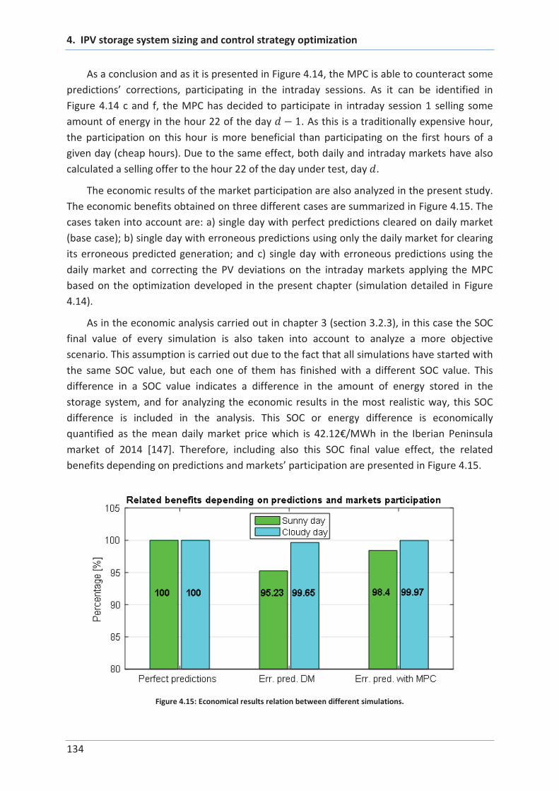
4. IPV storage system sizing and control strategy optimization
134
As a conclusion and as it is presented in Figure 4.14, the MPC is able to counteract some
predictions’ corrections, participating in the intraday sessions. As it can be identified in
Figure 4.14 c and f, the MPC has decided to participate in intraday session 1 selling some
amount of energy in the hour 22 of the day 1. As this is a traditionally expensive hour,
the participation on this hour is more beneficial than participating on the first hours of a
given day (cheap hours). Due to the same effect, both daily and intraday markets have also
calculated a selling offer to the hour 22 of the day under test, day .
The economic results of the market participation are also analyzed in the present study.
The economic benefits obtained on three different cases are summarized in Figure 4.15. The
cases taken into account are: a) single day with perfect predictions cleared on daily market
(base case); b) single day with erroneous predictions using only the daily market for clearing
its erroneous predicted generation; and c) single day with erroneous predictions using the
daily market and correcting the PV deviations on the intraday markets applying the MPC
based on the optimization developed in the present chapter (simulation detailed in Figure
4.14).
As in the economic analysis carried out in chapter 3 (section 3.2.3), in this case the SOC
final value of every simulation is also taken into account to analyze a more objective
scenario. This assumption is carried out due to the fact that all simulations have started with
the same SOC value, but each one of them has finished with a different SOC value. This
difference in a SOC value indicates a difference in the amount of energy stored in the
storage system, and for analyzing the economic results in the most realistic way, this SOC
difference is included in the analysis. This SOC or energy difference is economically
quantified as the mean daily market price which is 42.12€/MWh in the Iberian Peninsula
market of 2014 [147]. Therefore, including also this SOC final value effect, the related
benefits depending on predictions and markets’ participation are presented in Figure 4.15.
Figure 4.15: Economical results relation between different simulations.

4. IPV storage system sizing and control strategy optimization
135
These economic results are calculated based on the daily market, intraday markets and
positive and negative deviation penalties’ prices of Iberian Peninsula market in 2014 [147].
These values are explained in chapter 2.
The results show how the unique daily market participation considering erroneous
prediction can reduce the benefits around 5% in a sunny day and around 1% in a cloudy day,
while the MPC based intraday market participation improves these results. Applying the
MPC presented in this chapter (which optimizes the participation taking into account the
storage system SOC and its degradation, the PV prediction and the measured real generation
and the market prices forecast), the economic results are improved by around 3% in a sunny
day and maintains them around 99% in a cloudy day, compared to the second scenario.
Compared to the base case, both types of days (sunny and cloudy) have obtained around
99% of potential benefits. Assuming that the base case is the ideal scenario, this result (99%)
corresponds to a very positive result. This is due to the fact that the MPC has compensated
the PV deviation participating in some hours when there is no PV generation but the storage
system energy reserves have provided the possibility to sell some energy in other more
expensive hours of the day.
Therefore, the intraday market participation carried out by the MPC for reacting to PV
uncertainties provides the opportunity to obtain important benefits that justifies the
development of the control algorithm.
4.4. Market participation comparison with RB and optimal
control strategies
In this section the comparison of the both control strategies presented before, which
are related to their market participation, is carried out. The two presented control strategies
are the one based on rules (explained in Chapter 3) and the optimal one (explained in the
present chapter). The comparison is based on the market participation profile and the
economic results.
4.4.1. Market participation comparison
Regarding the market participation comparison, both sunny and cloudy days are
compared. In both cases, on the left side of the figures the rules based control strategy
results are presented while in the right side the results of the optimal control strategy are
presented. It is worth mentioning that each strategy is implemented in a different IPV power
plant (with different ESS capacity value), and for that reason, the objective of this
comparison is to analyze the philosophy of both strategies, more than the power
capabilities, that are influenced by the ESS.
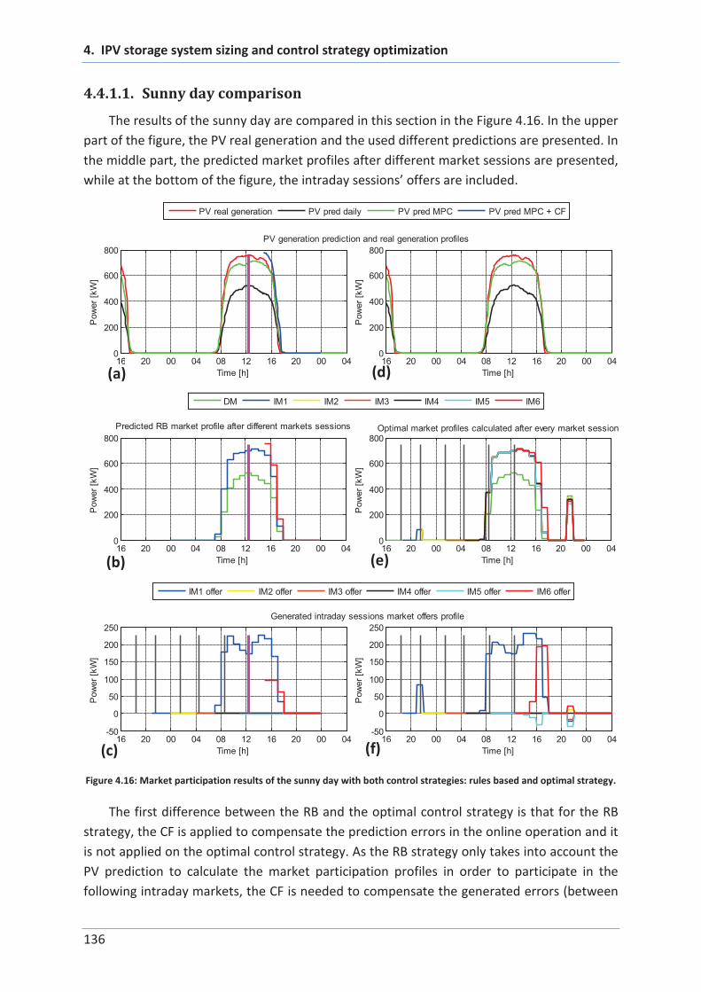
4. IPV storage system sizing and control strategy optimization
136
4.4.1.1. Sunny day comparison
The results of the sunny day are compared in this section in the Figure 4.16. In the upper
part of the figure, the PV real generation and the used different predictions are presented. In
the middle part, the predicted market profiles after different market sessions are presented,
while at the bottom of the figure, the intraday sessions’ offers are included.
Figure 4.16: Market participation results of the sunny day with both control strategies: rules based and optimal strategy.
The first difference between the RB and the optimal control strategy is that for the RB
strategy, the CF is applied to compensate the prediction errors in the online operation and it
is not applied on the optimal control strategy. As the RB strategy only takes into account the
PV prediction to calculate the market participation profiles in order to participate in the
following intraday markets, the CF is needed to compensate the generated errors (between
16 20 00 04 08 12 16 20 00 040
200
400
600
800
Time [h]
Pow
er
[kW
]
16 20 00 04 08 12 16 20 00 040
200
400
600
800Optimal market profiles calculated after every market session
Time [h]
Pow
er
[kW
]
DM IM1 IM2 IM3 IM4 IM5 IM6
16 20 00 04 08 12 16 20 00 04-50
0
50
100
150
200
250
Time [h]
Pow
er
[kW
]
IM1 offer IM2 offer IM3 offer IM4 offer IM5 offer IM6 offer
16 20 00 04 08 12 16 20 00 040
200
400
600
800
Time [h]
Pow
er
[kW
]
PV generation prediction and real generation profiles
16 20 00 04 08 12 16 20 00 040
200
400
600
800
Predicted RB market profile after different markets sessions
Time [h]
Pow
er
[kW
]
16 20 00 04 08 12 16 20 00 04-50
0
50
100
150
200
250
Generated intraday sessions market offers profile
Time [h]
Pow
er
[kW
]
PV real generation PV pred daily PV pred MPC PV pred MPC + CF
16 20
(a)
16 20
(b)
16
(c)
16 20
(d)
16 20
(e)
16-50
(f)

4. IPV storage system sizing and control strategy optimization
137
the PV prediction and real measurements). These errors (caused by PV generation deviation)
cause a variation of the SOC of the storage system, and as the optimization strategy also
takes into account this factor (the SOC), it does not need the CF to be able to compensate
the unexpected generated errors. The optimal control strategy, when it measures a lower
SOC value, it reduces the following markets’ participation in order to recover the SOC
reference value and indirectly, to avoid the penalties. This is the main difference regarding
the PV predictions for both strategies.
Analyzing the purely market participation operation, there is a relevant difference
between one strategy and the other. As it has been mentioned before, as the RB strategy
only takes into account the PV generation prediction in order to calculate the market
participation profile, it does not optimize the economic revenues; it only obtains the
revenues of the hours when there is PV generation. When the PV predictions change, the RB
control strategy changes its market participation profile, increasing or decreasing the
previously cleared profile. It can be observed that with a change in the PV prediction before
participating in the intraday session S1, the RB strategy proposes an incremental production
offer. This offer can be observed by the blue profile of Figure 4.16 c and f. The same effect
happens in the discrete state when the intraday session S6 is proposed, and it is presented
by the red profile of Figure 4.16 c and f.
Moreover, the optimal control strategy, as it takes into account the market prices, the
SOC of the storage system, and the produced error between the actual PV generation and
the prediction, is able to counteract these events, adapting the intraday sessions offers to
each optimal scenario. Also, as it considers the market prices, it decides to participate in the
most expensive hour of the day in all intraday sessions. But it is worth mentioning that as the
intraday session S1 starts with the most expensive hour of the day, the hour 22, between 9
p.m. and 10 p.m., the optimization of the revenues is still more important than the one
obtained with the RB strategy.
As a conclusion just for the control strategy comparison, it can be summarized that the
RB strategy is able to react to PV prediction changes but the optimal strategy not only takes
into account this information but is also able to react to PV generation changes, market
prices changes or SOC variations.
4.4.1.2. Cloudy day comparison
Analyzing the control strategies for the cloudy day, the overall results are similar with
some minor changes. The control strategies visual comparison is presented in Figure 4.17.
In this case, the error generated between the PV prediction and the real measurement,
results in a negative CF value. This causes a negative intraday session S6 offer based on the
RB strategy. The same effect is counteracted in the optimal strategy with a negative market
offer in the most expensive hour of the day, during hour 22, reducing the revenues but
avoiding more relevant penalties, obtaining the most beneficial scenario with this offer.

4. IPV storage system sizing and control strategy optimization
138
Figure 4.17: Market participation results of the cloudy day with both control strategies: rules based and optimal strategy.
The conclusions are the same as the ones stated for the sunny day, with a little
difference of sign for the intraday session S6 offer. This negative offer can be considered as a
purchase offer, as it is proposed by a generator. This operation is typical in renewable based
generators, in order to reduce their program due to more detailed predictions. Moreover, it
is worth mentioning an original effect appearing in the optimal strategy. As the optimal
scenario includes a relevant amount of energy offer at the hour 22, this offer serves as a
buffer for the predictions’ deviation, as it can be observed in the right side (optimal strategy)
results of Figure 4.17.
16 20 00 04 08 12 16 20 00 040
200
400
600
800
Time [h]
Pow
er
[kW
]
PV generation prediction and real generation profiles
16 20 00 04 08 12 16 20 00 040
200
400
600
800
Time [h]
Pow
er
[kW
]
Optimal market profiles calculated after every market session
16 20 00 04 08 12 16 20 00 04
-100
0
100
200
Time [h]
Pow
er
[kW
]
16 20 00 04 08 12 16 20 00 040
200
400
600
800
Time [h]
Pow
er
[kW
]
16 20 00 04 08 12 16 20 00 040
200
400
600
800
Time [h]
Pow
er
[kW
]
Predicted RB market profile after different markets sessions
16 20 00 04 08 12 16 20 00 04
-100
0
100
200
Time [h]
Pow
er
[kW
]
Generated intraday sessions market offers profile
DM IM1 IM2 IM3 IM4 IM5 IM6
IM1 offer IM2 offer IM3 offer IM4 offer IM5 offer IM6 offer
PV real generation PV pred daily PV pred MPC PV pred MPC + CF
16 20
(a)
16 20
(b)
16
(c)
16
(d)
16
(e)
16
(f)
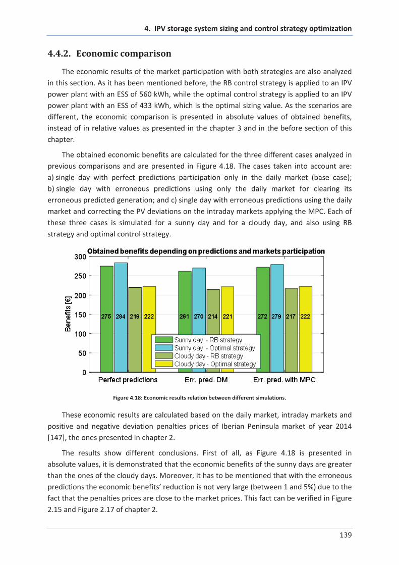
4. IPV storage system sizing and control strategy optimization
139
4.4.2. Economic comparison
The economic results of the market participation with both strategies are also analyzed
in this section. As it has been mentioned before, the RB control strategy is applied to an IPV
power plant with an ESS of 560 kWh, while the optimal control strategy is applied to an IPV
power plant with an ESS of 433 kWh, which is the optimal sizing value. As the scenarios are
different, the economic comparison is presented in absolute values of obtained benefits,
instead of in relative values as presented in the chapter 3 and in the before section of this
chapter.
The obtained economic benefits are calculated for the three different cases analyzed in
previous comparisons and are presented in Figure 4.18. The cases taken into account are:
a) single day with perfect predictions participation only in the daily market (base case);
b) single day with erroneous predictions using only the daily market for clearing its
erroneous predicted generation; and c) single day with erroneous predictions using the daily
market and correcting the PV deviations on the intraday markets applying the MPC. Each of
these three cases is simulated for a sunny day and for a cloudy day, and also using RB
strategy and optimal control strategy.
Figure 4.18: Economic results relation between different simulations.
These economic results are calculated based on the daily market, intraday markets and
positive and negative deviation penalties prices of Iberian Peninsula market of year 2014
[147], the ones presented in chapter 2.
The results show different conclusions. First of all, as Figure 4.18 is presented in
absolute values, it is demonstrated that the economic benefits of the sunny days are greater
than the ones of the cloudy days. Moreover, it has to be mentioned that with the erroneous
predictions the economic benefits’ reduction is not very large (between 1 and 5%) due to the
fact that the penalties prices are close to the market prices. This fact can be verified in Figure
2.15 and Figure 2.17 of chapter 2.

4. IPV storage system sizing and control strategy optimization
140
Analyzing the purely strategies’ results, in all cases the optimal strategy obtains better
results than the RB strategy, although the storage system of these scenarios is reduced by
23%, from 560 kWh to 433 kWh. This result demonstrates the advantage of the optimal
strategy that considers the whole system (PV predictions, PV measurement, SOC, electricity
market prices) compared to a strategy that only considers the PV predictions.
Regarding the use of the MPC, the results are also positives, due to the fact that in all
cases, with RB and mainly with optimal strategy, the economic benefits are very close to the
ideal scenario, which is the base case of perfect predictions. Moving the benefit closer to the
ideal scenario is the most interesting result that can be obtained in this study, and in this
case, the benefits have increased up to 99% of the ideal scenario.
Finally, assuming this benefits’ increase from erroneous prediction but considering the
use of MPC with the optimal strategy, the benefits’ increase every year about 3000€, in
addition to the ESS reduction.
4.5. Conclusions
This forth chapter contains the main contributions of the present PhD work. The market
participation based on the optimal control strategy and the optimal storage system sizing
are the objectives that have been presented in the general introduction, and they have been
explained and developed in this chapter.
First, the procedure of the optimization has been presented and explained in detail. This
procedure includes the details for carrying out both optimal sizing and control of the
selected application. The co-optimization process includes the problem identification, the
objective function explanation, the design variables selection and lower and upper bound
identification, constraints analysis considering inequalities and equalities, algorithm
application and simulation execution process explanation. Within these equations the model
of the storage system degradation is included (considering both cycling and calendar
degradation) together with its operation equation and market operation behavior equation.
The objective function includes some terms of the whole economic model presented in
chapter 2. The main contribution of the proposed optimization procedure is that both sizing
and control strategies variables have been included, having the possibility to run a single
optimization which calculates the optimal sizing with the optimal control strategy.
After the model explanation, the sizing and control strategy steps have been presented,
considering the two stages that need to be followed, which are the design stage of the IPV
power plant, defining the size of the storage system; and the operation stage where the size
of the storage system has been already fixed and the optimal control strategy has been
calculated in order to obtain the maximum economic revenues from the market
participation of the whole IPV power plant.
4. IPV storage system sizing and control strategy optimization
141
Once these stages have been determined, the results of the optimization have been
presented, analyzing the results for obtaining the optimal sizing, together with the results of
the control strategy. This control strategy has been afterwards included in the market
participation based on the MPC, where the operation has been described and the results
related to this participation have been also presented. These results are related to each
market participation offers (daily market and the six sessions of the intraday market) and
also related to the economic benefits. The market participation has been presented for two
different days, a sunny and a cloudy day, demonstrating the correct operation of the optimal
control strategy in both cases and the relevant improvement gap obtained from the daily
market participation case, as presented in Figure 4.15.
Considering that the base case (perfect predictions) is the ideal scenario, reaching 99%
of that value represents a very positive result. This is due to the fact that the MPC has
compensated the PV deviation participating in some hours when there is no PV generation
but the storage system energy reserves have provided the possibility to sell some energy in
other more expensive hours of the day. Therefore, the intraday market participation carried
out by the MPC for reacting to PV uncertainties has provided the opportunity to obtain
important benefits that justifies the development of the control algorithm.
Finally, the results of the presented optimization process and market participation have
been compared to the ones presented in chapter 3 where the control strategy has been
developed based on the analyzed RB strategy. This comparison shows the good results of the
market participation based on rules, and the still better results of the proposed optimization
process. The economic results have been improved from the cases where the MPC is not
used, and also from the cases where the optimal strategy is not used. Thus, the results
applying the MPC with the optimal control strategy have reached also 99% of the ideal
scenario results, which is an important benefits increase compared to a case without those
algorithms. This case of optimal based MPC has increased the benefits while it has reduced
the ESS size of 23%, demonstrating that the optimization based MPC permits to increase the
benefits in a considerable way.


5 Real time validation of
the rules based and
the optimal control
strategies


5. Real time validation of the rules based and the optimal control strategies
145
5. Real time validation of the rules
based and the optimal control
strategies
This fifth chapter presents the real time validation carried out in a Hardware-in-the-Loop
(HIL) platform. The objective of this chapter is to demonstrate the possibility of
implementation of the control strategies developed and described in chapters 3 and 4 to
participate in the electricity market in a commercial real-time IPV controller device.
In the fourth chapter, the optimal sizing of the energy storage system that composes an
IPV power plant has been calculated. The obtained results show a lifetime of 8 years (as it is
presented in Figure 4.8 of chapter 4), working as the optimization required conditions. These
conditions are the ones that calculate the optimal control strategy. This strategy is calculated
to extend the lifetime of the storage system and, in the general point of view, it is also
calculated to obtain the greatest benefits of the whole system during the complete lifetime
of the IPV power plant.
Unfortunately, neither the optimal sizing nor the optimal strategy can be validated in
some days, weeks or months, because the optimal strategy is calculated for the whole
lifetime of the system, which is of several years. This validation horizon exceeds the time
horizon of this PhD work. Therefore, the optimal sizing and the economic optimality of the
control strategy cannot be directly validated in the scope of this PhD.
Nevertheless, the real-time operation conditions of the optimal control strategy and the
rules based (RB) control strategy can be validated and it is validated in this chapter. Thus, the
algorithms of the control strategies are conceptually validated. Moreover, in the case of the
optimal control strategy, at every discrete state, an optimization must be carried out, and
the possibility to do these optimizations as fast as the selected discrete state is also
demonstrated.
Furthermore, from the simulation of a given control strategy to its application in a real
system, different steps should be followed. The real time validation is an intermediate step
that facilitates the transition from the simulation to the real application.
This validation chapter is composed by the general description of the validation
platform, the description of the market participation results with the RB control strategy,
and the description of the market participation results with the optimal control strategy.
5.1. General description of the validation platform
In the present real time validation, the used platform is composed with a simulated IPV
power plant controlled by a real industrial controller, a PLC (Programmable Logic Controller).

5. Real time validation of the rules based and the optimal control strategies
146
This controller is managing the real PV power plant presented in chapter 2. It is an actual
hardware part of the system, programmed and constructed to be able to control a real IPV
power plant. Therefore, the validation platform used in this PhD work is very close to the
real application, due to the fact that the implemented control strategies can be directly
uploaded in the PLC. An overall picture that presents the whole platform is shown in Figure
5.1.
Figure 5.1: Real time validation platform picture.
5.2. Results of the market participation based on RB strategy
In this section, the possibility to run the RB control strategy in the Hardware-in-the-Loop
platform is validated. To do so, firstly, the validation platform architecture is described and
secondly, the results of a sunny and a cloudy day’s real time operation are presented,
validating in this way, the possibility to participate in electricity markets with the RB control
strategy.
5.2.1. Description of the validation platform architecture
From the complete platform presented in Figure 5.1, not all the devices are used for the
validation of the RB control strategy. In this case, the used devices and their main functions
are summarized as follows:

5. Real time validation of the rules based and the optimal control strategies
147
PIP8: IPV power plant and grid electric models real time emulation.
PLC: IPV power plant control based on market cleared references and IPV power
plant measurements.
Main computer: control references and IPV power plant measurements
monitoring, the PV prediction update and the market participation.
Therefore, the diagram to carry out this validation is the one presented in Figure 5.2.
*
Plant controller
Generation planning
RB5
control
strategy
PV forecast
(1:24)
Market forecastEoffered(k)
MPC
RB5
control
strategy
PV forecast
(k:24)
Ecleared(k)
Eoffered(k)
Ecleared(k)
Pbat(k)
Pbat meas (k)SOC
PPV meas (k)T
ime s
equence
DC
AC
PV
PV local controller
Battery localcontroller
BMS
DC
AC
Battery
IPV plant Grid
PCC
comms
Plantcontroller
Pgrid(k)
Online operation
Market
Daily market
Pgrid(k)
*
IMj
DM
DM
IMj
IMj))))
Intraday markets
...1
26
coffered(k)DM
ccleared(k)DM
1/hourEcleared(k)
ccleared(k)
coffered(k)IMj
ccleared(k)
PLC task:
- IPV power plant control based on
market cleared references
PLC task:
- IPV power plant control based on
market cleared references
Power
referencesMeasure-
ments
Main computer tasks:
- Control references monitoring
- IPV power plant measurements monitoring
- PV prediction update
- Market participation
Measurements: Pgrid, PPV, Pbat, SOC, SOH
Power references: Pmkt, Pbat
Market cleared
references
PIP8 task:
- Real time execution of the IPV power plant
model
DC
AC
PV
PV local controller
Battery localcontroller
BatteryBatteryBMS
DC
AC
Battery
IPV plant Grid
PCC
comms
Plantcontroller
Market
Pgrid(k) PIP8 task:
- Real time execution of the IPV power plant
model
Figure 5.2: Market participation validation scenario based on the RB control strategy.
As it is shown in Figure 5.2, the PLC controls the IPV power plant model (presented in
chapter 3) included in the PIP8 and the IPV power plant measurements are sent back to the
PLC. The main computer carries out the market participation process and, based on this

5. Real time validation of the rules based and the optimal control strategies
148
process, the market cleared references are transferred to the PIP8, in order to control the
IPV power plant providing the cleared power references. The main computer also manages
the monitoring of all important parameters as the market cleared references, the power
references sent from PLC to the PIP8 and the IPV power plant measurements ( , ,
, , , ).
In this validation step, the electrical parameters of the IPV power plant model included
in the PIP8 are the ones summarized in Table 5.1.
Table 5.1: Implemented IPV power plant electrical parameters.
Parameter description Value
Maximum power of PV inverter 1 MW
Maximum power of battery inverter 1 MW
Maximum battery charge power 1 MW
Maximum battery discharge power 1 MW
Battery nominal capacity 560 kWh
Limited maximum SOC 90%
Limited minimum SOC 10%
Initial SOC 50%
Initial SOH 100%
Once the IPV power plant electrical parameters have been defined, the simulation
characteristics must be explained. In this case, as the market participation is carried out
based on the PV predictions and without taking into account the storage system state of
charge of the IPV power plant, the market participation profile is just the same compared
with the one calculated in chapter 3. For that reason, and considering that the cleared
profile is centered in the 13 hours of the middle of the day (from 6:00 am to 19:00 pm), the
real time simulation is carried out considering a time horizon of 15 hours. To maintain the
real scope, each real minute is simulated as a second. Therefore, the 15 hours of the real
time validation are simulated in 15 minutes. The details of the simulation characteristics are
presented in Table 5.2.

5. Real time validation of the rules based and the optimal control strategies
149
Table 5.2: Simulation characteristics of the market participation based on RB strategy.
Parameter description Value
Ts 0.25ms
Real time simulation length 900s
Real reference time length 15 hours
Starting time 5:00 am
5.2.2. Results of a sunny day market participation process
The results of a sunny day market participation process are presented in this section.
Firstly, the inputs of the process are presented. As the market participation process is
calculated based on the PV predictions, the market profile which is the reference for the IPV
power plant is calculated as presented in chapter 3. The other input is the real PV
generation, which is also presented in chapter 3. Both profiles for a representative sunny day
are depicted in Figure 5.3.
Figure 5.3: Market cleared and the PV generation inputs of the validation for a sunny day.
As it can be shown in Figure 5.3, the market profile is below the PV generation profile
during the middle day hours and this difference is counteracted in the final hours of the day,
with an increased market profile.
Once the inputs of the model have been introduced, the operation carried out in the
validation scenario is presented. The included profiles are the ones included in the last figure

5. Real time validation of the rules based and the optimal control strategies
150
(Figure 5.3, and ) together with the storage system power profile ( ) and the
generated IPV power plant output power profile or grid provided power profile ( ).
These results are presented in Figure 5.4.
Figure 5.4: Sunny day operation based on RB control strategy.
Figure 5.5 represents the SOC variation of the storage system for providing the power
profile shown in Figure 5.4. Both figures must be jointly analyzed to understand the whole
day operation.
Figure 5.5: Storage system SOC variation corresponding to a sunny day operation based on RB control strategy.
As it can be extracted from Figure 5.4, the IPV power plant perfectly follows the market
profile every time the battery is within its operation condition bounds (included in Table
4.1). In the morning hours, as the battery SOC starting point is considered to be 50% of SOC,
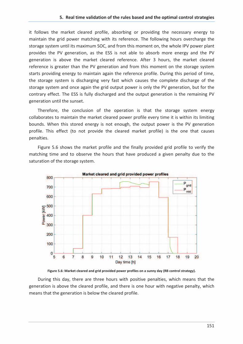
5. Real time validation of the rules based and the optimal control strategies
151
it follows the market cleared profile, absorbing or providing the necessary energy to
maintain the grid power matching with its reference. The following hours overcharge the
storage system until its maximum SOC, and from this moment on, the whole IPV power plant
provides the PV generation, as the ESS is not able to absorb more energy and the PV
generation is above the market cleared reference. After 3 hours, the market cleared
reference is greater than the PV generation and from this moment on the storage system
starts providing energy to maintain again the reference profile. During this period of time,
the storage system is discharging very fast which causes the complete discharge of the
storage system and once again the grid output power is only the PV generation, but for the
contrary effect. The ESS is fully discharged and the output generation is the remaining PV
generation until the sunset.
Therefore, the conclusion of the operation is that the storage system energy
collaborates to maintain the market cleared power profile every time it is within its limiting
bounds. When this stored energy is not enough, the output power is the PV generation
profile. This effect (to not provide the cleared market profile) is the one that causes
penalties.
Figure 5.6 shows the market profile and the finally provided grid profile to verify the
matching time and to observe the hours that have produced a given penalty due to the
saturation of the storage system.
Figure 5.6: Market cleared and grid provided power profiles on a sunny day (RB control strategy).
During this day, there are three hours with positive penalties, which means that the
generation is above the cleared profile, and there is one hour with negative penalty, which
means that the generation is below the cleared profile.

5. Real time validation of the rules based and the optimal control strategies
152
The economic evaluation of this market participation based on the market prices of the
Iberian Peninsula electricity markets is the one presented in chapter 3, in section 3.2.3 and in
Figure 3.13 (sunny day).
5.2.3. Results of a cloudy day market participation process
As in the sunny day’s market participation process, the results of the cloudy day are also
presented in order to analyze the market participation process and the IPV power plant
operation.
As in the previous case, the inputs of the market participation based on the RB control
strategy are the market cleared profile and the PV generation profile presented in Figure 5.7.
Figure 5.7: Market cleared and the PV generation inputs of the validation for a cloudy day.
In this case, the generation of several hours of the day is below the market cleared
reference, with important variability and restrictive peaks that it is supposed that will rapidly
discharge the storage system.
The operation of the IPV power plant based on the RB control strategy is presented in
Figure 5.8. As in the sunny day case, this figure depicts the PV generation profile, the market
cleared profile, the ESS power profile and the IPV power plant output power profile or grid
provided profile.
Together with this figure, the following Figure 5.9 shows the storage system SOC
variation, which corresponds to the power profile needed and presented in Figure 5.8.

5. Real time validation of the rules based and the optimal control strategies
153
Figure 5.8: Cloudy day operation based on RB control strategy.
Figure 5.9: Storage system SOC variation corresponding to a cloudy day operation based on RB control strategy.
In this case, as in the previous case, while the battery SOC is within its limits, the grid
output power of the whole IPV power plant matches perfectly with the cleared reference
power profile. This happens from the dawn until 1 pm. During this period of time, there are
several peaks which demand an important power requirement to the storage system (with a
maximum peak about 400 kW). The storage system is able to provide this peak and also to
vary its operation from providing energy to continuously absorbing energy as it can be
verified between 11 am and 1 pm. Around 1 pm, the storage system is completely
discharged, and for that reason the output power of the IPV power plant is directly the PV
generation. At 2 pm and at 2.45 pm, there are two little peaks of PV generation that
overpass the market cleared reference and they are used to charge the ESS. From 3 pm on,
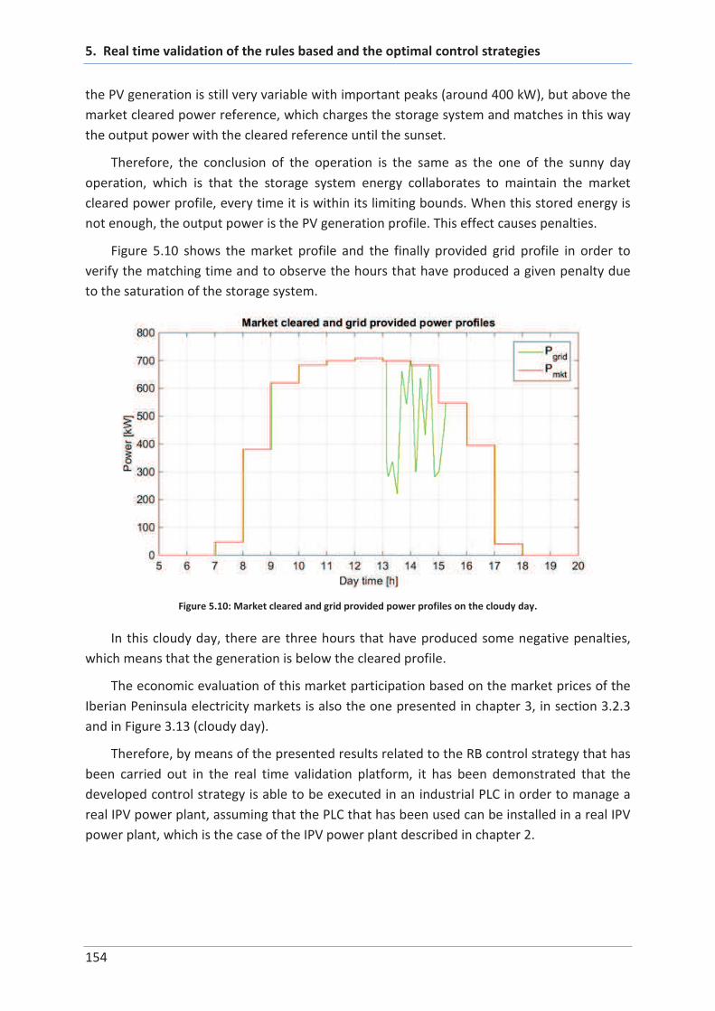
5. Real time validation of the rules based and the optimal control strategies
154
the PV generation is still very variable with important peaks (around 400 kW), but above the
market cleared power reference, which charges the storage system and matches in this way
the output power with the cleared reference until the sunset.
Therefore, the conclusion of the operation is the same as the one of the sunny day
operation, which is that the storage system energy collaborates to maintain the market
cleared power profile, every time it is within its limiting bounds. When this stored energy is
not enough, the output power is the PV generation profile. This effect causes penalties.
Figure 5.10 shows the market profile and the finally provided grid profile in order to
verify the matching time and to observe the hours that have produced a given penalty due
to the saturation of the storage system.
Figure 5.10: Market cleared and grid provided power profiles on the cloudy day.
In this cloudy day, there are three hours that have produced some negative penalties,
which means that the generation is below the cleared profile.
The economic evaluation of this market participation based on the market prices of the
Iberian Peninsula electricity markets is also the one presented in chapter 3, in section 3.2.3
and in Figure 3.13 (cloudy day).
Therefore, by means of the presented results related to the RB control strategy that has
been carried out in the real time validation platform, it has been demonstrated that the
developed control strategy is able to be executed in an industrial PLC in order to manage a
real IPV power plant, assuming that the PLC that has been used can be installed in a real IPV
power plant, which is the case of the IPV power plant described in chapter 2.

5. Real time validation of the rules based and the optimal control strategies
155
5.3. Results of the market participation based on optimal
strategy
In this section another configuration of the platform is presented in order to validate the
possibility of running the optimal control strategy to participate in electricity markets. To do
so, the tertiary computer presented in Figure 5.1 is used to execute the optimization
process. Together with the new platform configuration and its description, the market
participation process results corresponding to a sunny and a cloudy day are presented.
5.3.1. Description of the validation platform architecture
The necessary devices to carry out the present validation are the ones included in the
following list, where their main tasks are also summarized:
PIP8: IPV power plant and grid electric models real time emulation.
PLC: IPV power plant control based on market cleared references and IPV power
plant measurements.
Main computer: control references and IPV power plant measurements
monitoring, the PV prediction update and the market participation
communications (from the tertiary computer to the PLC).
Tertiary computer: it runs the developed optimization process (chapter 4) to
calculate the optimal market participation offers and battery power references.
Figure 5.11 presents a diagram explaining the task of each device and the information
sent from one device to the others. Therefore, this scenario presents a real market
participation system, which is able to manage a real IPV power plant and is also prepared to
participate in electricity markets through the tertiary computer.

5. Real time validation of the rules based and the optimal control strategies
156
*
Plant controller
Generation planning
PV forecast
(1:24)
Market forecastEoffered(k)
MPC
PV forecast
(k:24)
Ecleared(k)
Eoffered(k)
Ecleared(k)
Pbat(k)
Pbat meas (k)SOC(k)
PPV meas (k)
Tim
e s
equence
DC
AC
PV
PV local controller
Battery localcontroller
BMS
DC
AC
Battery
IPV plant Grid
PCC
comms
Plantcontroller
Pgrid(k)
Online operation
Market
Daily market
Pgrid(k)
*
IMj
DM
DM
IMj
IMj))))))))))))
Intraday markets
...1
26
coffered(k)DM
ccleared(k)DM
1/hourEcleared(k)
ccleared(k)
coffered(k)IMj
ccleared(k)
LP Optimization
ESS fixed
Optimal operation
LP Optimization
ESS fixed
Optimal operation
Market forecast
PLC task:
- IPV power plant control based on
market cleared references
PLC task:
- IPV power plant control based on
market cleared references
Power
referencesMeasure-
ments
Main computer tasks:
- Control references monitoring
- IPV power plant measurements monitoring
- PV prediction update
- Market participation
Market cleared
references
PIP8 task:
- Real time execution of the IPV power plant
model
DC
AC
PV
PV local controller
Battery localcontroller
BatteryBatteryBMS
DC
AC
Battery
IPV plant Grid
PCC
comms
Plantcontroller
Market
Pgrid(k) PIP8 task:
- Real time execution of the IPV power plant
model
Tertiary computer task:
- Run optimization process to calculate the optimal
market participation and battery power reference
PV prediction,
SOC, SOH
Optimal
referencesMeasurements: Pgrid, PPV, Pbat, SOC, SOH
Power references: Pmkt, Pbat
Figure 5.11: Market participation validation scenario based on the optimal control strategy.
As it can be shown in Figure 5.11, the PLC controls the IPV power plant model included
in the PIP8 as it has been presented in chapter 4. The measurements of the IPV power plant
are sent back to the PLC in order to close the control loop. The main computer sends to the
PLC the market cleared references based on the market participation process optimally
executed in the tertiary computer. As it has been mentioned before, this optimization based
market participation process presented and analyzed in chapter 4 is the main contribution of
this PhD work. This market participation is carried out taking into account some internal
variables of the IPV power plant as the PV prediction, PV real measurement, and the SOC
and the SOH of the storage system. Therefore, based on this optimization based market
participation process the market cleared optimal references are transferred from the
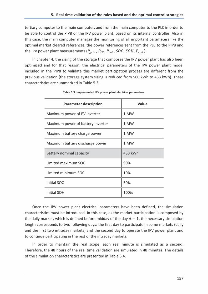
5. Real time validation of the rules based and the optimal control strategies
157
tertiary computer to the main computer, and from the main computer to the PLC in order to
be able to control the PIP8 or the IPV power plant, based on its internal controller. Also in
this case, the main computer manages the monitoring of all important parameters like the
optimal market cleared references, the power references sent from the PLC to the PIP8 and
the IPV power plant measurements ( , , , , , ).
In chapter 4, the sizing of the storage that composes the IPV power plant has also been
optimized and for that reason, the electrical parameters of the IPV power plant model
included in the PIP8 to validate this market participation process are different from the
previous validation (the storage system sizing is reduced from 560 kWh to 433 kWh). These
characteristics are summarized in Table 5.3.
Table 5.3: Implemented IPV power plant electrical parameters.
Parameter description Value
Maximum power of PV inverter 1 MW
Maximum power of battery inverter 1 MW
Maximum battery charge power 1 MW
Maximum battery discharge power 1 MW
Battery nominal capacity 433 kWh
Limited maximum SOC 90%
Limited minimum SOC 10%
Initial SOC 50%
Initial SOH 100%
Once the IPV power plant electrical parameters have been defined, the simulation
characteristics must be introduced. In this case, as the market participation is composed by
the daily market, which is defined before midday of the day 1, the necessary simulation
length corresponds to two following days: the first day to participate in some markets (daily
and the first two intraday markets) and the second day to operate the IPV power plant and
to continue participating in the rest of the intraday markets.
In order to maintain the real scope, each real minute is simulated as a second.
Therefore, the 48 hours of the real time validation are simulated in 48 minutes. The details
of the simulation characteristics are presented in Table 5.4.

5. Real time validation of the rules based and the optimal control strategies
158
Table 5.4: Simulation characteristics of the market participation based on optimal strategy.
Parameter description Value
Ts 0.5ms
Real time simulation length 2880s
Real reference time length 48 hours
5.3.2. Results of a sunny day market participation process
Once described the real time validation platform where the market participation based
on optimal control strategy is applied, in this section, the results of a sunny day market
participation process are presented.
In this case, the inputs of the IPV power plant are the market cleared profiles and the PV
generation profile. The market cleared profiles are the ones that have been calculated in the
tertiary computer to obtain the optimal market participation process. Although these
profiles are presented all together, each one of them is obtained in a different moment with
different storage system and PV predictions conditions. The market cleared profiles obtained
in the tertiary computer based on the optimal market participation are presented in Figure
5.12.
Figure 5.12: Optimal daily and intraday markets participation calculated in the tertiary computer (sunny day).
As it can be concluded from Figure 5.12, the daily market clears a typical PV generation
bell (around 500 kW) and the first session of the intraday market clears another important
generation area (around 200 kW during the whole part of the day). Moreover, as the

5. Real time validation of the rules based and the optimal control strategies
159
intraday 1 is able to participate in the last three hours of the previous day and one of these
three hours is the most expensive hour of the day, it calculates an offer from the energy
stored in the ESS. Apart from that, all markets reserve an important energy amount for the
most expensive hour of the day under consideration (hour 22). That is why all markets make
an offer in this hour. The last market that operates in this day is the intraday 1 of the
following day, which in this case has reduced the market offer of the hour 22 due to the SOC
of the storage system.
Once the market participation profiles have been presented, the operation carried out
in the validation scenario is described. Four profiles are included: the addition of the market
participation profiles (from Figure 5.12) that compose the market cleared reference profile;
the PV power profile; the storage system power profile; and the generated IPV power plant
output power profile (or grid provided power profile). These results are presented in Figure
5.13. Figure 5.14 represents the SOC variation of the storage system for providing the power
profile shown in Figure 5.13.
Figure 5.13: Sunny day operation based on the optimal control strategy.

5. Real time validation of the rules based and the optimal control strategies
160
Figure 5.14: Storage system SOC variation corresponding to a sunny day operation based on the optimal control strategy.
Both figures (Figure 5.13 and Figure 5.14) must be jointly analyzed in order to
understand the whole day operation. Once again, as in the previous validation, it can be
stated that the IPV power plant perfectly follows the market profile while the battery is
within its operation condition bounds (included in Table 5.3).
First of all, as the most beneficial hour is the hour 22, the IPV power plant provides
some amount of energy discharging in this way the ESS. It is not a complete discharge in
order to be able to react in the presence of any unknown effect and for that reason the
optimal strategy decides to discharge the storage system until the 30% of SOC.
In the morning hours, the first objective is to recharge the storage system for future
events. So, the IPV power plant output power follows the market cleared profile, absorbing
or providing the necessary energy to maintain the grid power matching with its reference
while it is also charging. From 9 am on, there is an unexpected PV generation that
overcharges the storage system until its maximum SOC value. The next intraday market to
react to this effect is the intraday 6 that is resolved around midday but that starts in
operation at 3 pm. As it can be verified in Figure 5.12, the intraday 6 has an important offer
to resolve this fact.
During this period of time, as the PV generation is maintained above the cleared market
profile, the storage system is maintained saturated in its upper bound. Moreover, the whole
IPV power plant directly provides the PV generation as the ESS is not able to absorb more
energy.
At 3pm the last market starts in operation (the intraday 6) and the storage system
discharges its energy providing a greater market value than the one of the PV generation
while maintaining again the grid provided profile to the cleared one until the sunset. At this
point, the energy of the storage system is reserved again to the most expensive hour of the

5. Real time validation of the rules based and the optimal control strategies
161
day (hour 22), and at this period of time, it provides an amount of energy to discharge the
storage system at the most expensive hour of the day.
Therefore, the conclusion of the operation is that the most expensive hour of the day is
selected to discharge an important part of the storage system in order to obtain the highest
benefit, which shows how the optimal market participation has been searched.
The last figure to verify the validation of the market participation based on the optimal
control strategy is the one presented in Figure 5.15. This figure shows the optimal market
profile and the finally provided grid profile to verify the matching time and to observe the
hours that have produced a given penalty due to the saturation of the storage system.
Figure 5.15: Market cleared and grid provided power profiles on a sunny day (optimal control strategy).
In this day, there are several hours that have produced some positive penalties, which
means that the generation is above the cleared profile. This is due to an unexpected PV
generation excess and it is counteracted in the next intraday market session. Moreover, the
market participation has selected the most expensive hour of the day, which maximizes the
obtained benefits.
The economic evaluation of this market participation based on the market prices of the
Iberian Peninsula electricity markets is the one presented in chapter 4, in section 4.3.2 and in
Figure 4.15 (sunny day).
5.3.3. Results of a cloudy day market participation process
As in a sunny day’s market participation process, the results of a cloudy day are also
presented here, analyzing the same power profiles. They have been analyzed starting from
the optimal market participation of all markets (daily and intraday markets) and finishing
with the grid provided power profile in order to analyze the economic aspects of the
presented optimal market participation.
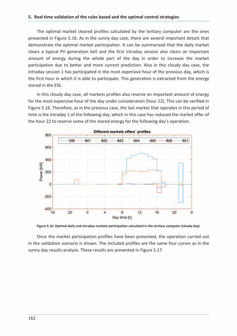
5. Real time validation of the rules based and the optimal control strategies
162
The optimal market cleared profiles calculated by the tertiary computer are the ones
presented in Figure 5.16. As in the sunny day case, there are several important details that
demonstrate the optimal market participation. It can be summarized that the daily market
clears a typical PV generation bell and the first intraday session also clears an important
amount of energy during the whole part of the day in order to increase the market
participation due to better and more current prediction. Also in this cloudy day case, the
intraday session 1 has participated in the most expensive hour of the previous day, which is
the first hour in which it is able to participate. This generation is extracted from the energy
stored in the ESS.
In this cloudy day case, all markets profiles also reserve an important amount of energy
for the most expensive hour of the day under consideration (hour 22). This can be verified in
Figure 5.16. Therefore, as in the previous case, the last market that operates in this period of
time is the intraday 1 of the following day, which in this case has reduced the market offer of
the hour 22 to reserve some of the stored energy for the following day’s operation.
Figure 5.16: Optimal daily and intraday markets participation calculated in the tertiary computer (cloudy day).
Once the market participation profiles have been presented, the operation carried out
in the validation scenario is shown. The included profiles are the same four curves as in the
sunny day results analysis. These results are presented in Figure 5.17.
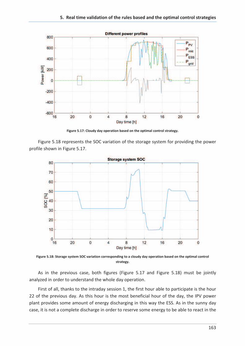
5. Real time validation of the rules based and the optimal control strategies
163
Figure 5.17: Cloudy day operation based on the optimal control strategy.
Figure 5.18 represents the SOC variation of the storage system for providing the power
profile shown in Figure 5.17.
Figure 5.18: Storage system SOC variation corresponding to a cloudy day operation based on the optimal control
strategy.
As in the previous case, both figures (Figure 5.17 and Figure 5.18) must be jointly
analyzed in order to understand the whole day operation.
First of all, thanks to the intraday session 1, the first hour able to participate is the hour
22 of the previous day. As this hour is the most beneficial hour of the day, the IPV power
plant provides some amount of energy discharging in this way the ESS. As in the sunny day
case, it is not a complete discharge in order to reserve some energy to be able to react in the
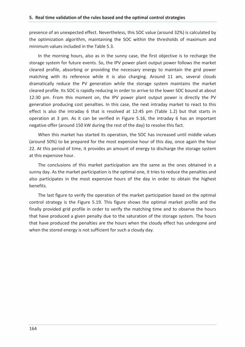
5. Real time validation of the rules based and the optimal control strategies
164
presence of an unexpected effect. Nevertheless, this SOC value (around 32%) is calculated by
the optimization algorithm, maintaining the SOC within the thresholds of maximum and
minimum values included in the Table 5.3.
In the morning hours, also as in the sunny case, the first objective is to recharge the
storage system for future events. So, the IPV power plant output power follows the market
cleared profile, absorbing or providing the necessary energy to maintain the grid power
matching with its reference while it is also charging. Around 11 am, several clouds
dramatically reduce the PV generation while the storage system maintains the market
cleared profile. Its SOC is rapidly reducing in order to arrive to the lower SOC bound at about
12:30 pm. From this moment on, the IPV power plant output power is directly the PV
generation producing cost penalties. In this case, the next intraday market to react to this
effect is also the intraday 6 that is resolved at 12:45 pm (Table 1.2) but that starts in
operation at 3 pm. As it can be verified in Figure 5.16, the intraday 6 has an important
negative offer (around 150 kW during the rest of the day) to resolve this fact.
When this market has started its operation, the SOC has increased until middle values
(around 50%) to be prepared for the most expensive hour of this day, once again the hour
22. At this period of time, it provides an amount of energy to discharge the storage system
at this expensive hour.
The conclusions of this market participation are the same as the ones obtained in a
sunny day. As the market participation is the optimal one, it tries to reduce the penalties and
also participates in the most expensive hours of the day in order to obtain the highest
benefits.
The last figure to verify the operation of the market participation based on the optimal
control strategy is the Figure 5.19. This figure shows the optimal market profile and the
finally provided grid profile in order to verify the matching time and to observe the hours
that have produced a given penalty due to the saturation of the storage system. The hours
that have produced the penalties are the hours when the cloudy effect has undergone and
when the stored energy is not sufficient for such a cloudy day.

5. Real time validation of the rules based and the optimal control strategies
165
Figure 5.19 Market cleared and grid provided power profiles on a cloudy day (optimal control strategy).
In this day, there are three hours that have produced some negative penalties, which
means that the generation is below the cleared profile. This is due to the unexpected PV
generation reduction caused by the clouds effect. This fact is counteracted in the next
intraday market session. Moreover, the market participation has selected the most
expensive hour of the day (hour 22), which maximizes the obtained benefits.
The economic evaluation of this market participation based on the market prices of the
Iberian Peninsula electricity markets is the one presented in chapter 4, in section 4.3.2 and in
Figure 4.15 (cloudy day).
As a conclusion, by means of the presented results related to the optimal control
strategy that has been carried out in the real time platform, it has been demonstrated that
the developed optimal control strategy is able to be executed in an industrial PLC in order to
manage a real IPV power plant. Moreover, this optimal control strategy, that increases the
obtained benefits, is able to increase the viability of the IPV power plants, increasing in this
way, the renewable resources rate in energy mixes.
5.4. Conclusions
In this fifth chapter, the real time validation of the proposed market participation
process has been presented. The objective of this validation is to demonstrate the possibility
of implementation of the developed control strategies to participate in the electricity market
in a commercial real-time IPV controller device.
Two different control strategies to manage the market participation process have been
validated. The first one is the RB control strategy extensively described in chapter 3 and the

5. Real time validation of the rules based and the optimal control strategies
166
second one is the optimal control strategy precisely detailed in chapter 4. Both strategies
have been implemented in a real time validation platform.
The strength of the present validation comes from the real PLC that has been used in
the platform, which provides the validation of the intermediate step from the simulation
based algorithms to the application of those algorithms in real systems. Thus, it can be
stated that the validation has been carried out in a scenario very close to the real
application, considering an IPV power plant real time conditions.
It has also been stated that the optimal storage system sizing cannot be verified nor
validated due to the fact that the validation horizon of this process exceeds the time horizon
of this PhD work, but the important fact has been the demonstration of the possibility to
participate in electricity markets and the control of the IPV power plant based on the
presented participation and control strategies.
Moreover, the simulations carried out in a single computer have been validated in a
hardware-in-the-loop system where the obtained results have been the same as the ones
obtained in the simulation step. This has been performed for both the RB control strategy
and the optimal control strategy, showing that the real time operation does not includes any
unexpected effect or delay in the whole IPV power plant.
In addition to that, in the optimal control strategy validation, the time steps of the
different markets (the daily one and the six sessions of the intraday market) have been
respected sending an offer and assuming a cleared power reference for the different horizon
of each market. This fact increases the reality of the current market participation application
managed by an IPV power plant.
As a main conclusion, the validation of the proposed market participation has been
demonstrated, offering the possibility to participate in electricity markets with the
developed process from today on. Moreover, the possibility to implement these strategies in
the same PLC that is controlling a real IPV power plant provides the reliability to the
proposed control strategies, both RB and optimal control strategies.
And, finally, as the optimal control strategy is also able to be implemented in a real IPV
power plant, it is able to increase the economic benefits of the IPV power plants increasing,
in this way, the renewable resources’ rate in energy mixes.

Conclusions and future
research lines

Conclusions and future research lines
169
Conclusions and future research lines
In this PhD study the optimal participation of IPV power plants in electricity markets has
been developed. To do so, BESS storage capability is used to reduce variability and provide
to the entire IPV power plant an increase in controllability. Based on such a system, a PV
power plant when associated with an energy storage system may provide different control
strategies to participate efficiently in the electricity markets. Moreover, a co-optimization
procedure has been developed to optimize both the sizing and the energy management
strategy in the same optimization step. The developed control strategies are included in an
innovative market participation process through the model predictive control, which
provides the possibility to participate in daily and intraday electricity markets.
The system on which the controllability of the whole IPV power plant must be relied, the
ESS, has a different operation behavior depending on how it is used. For that reason it is the
main and the most complicated system to be determined. That is why its sizing and control
has to be optimized to obtain the maximum benefits of the whole IPV power plant.
Therefore, the main contribution of this PhD is the development of a market
participation process where the ESS sizing and its control strategy is optimized to maximize
revenues based on the participation in the intraday markets by means of the model
predictive control, MPC.
Other contributions of this PhD study are summarized as follows:
A battery energy storage technology selection methodology proposition. After an
analysis about the most often used battery energy storage technologies, a selection
methodology has been proposed and applied to obtain that Lithium-ion technology is the
most appropriate storage technology to be used for the application considered in the
present PhD work.
The identification of the most beneficial electricity markets to participate in by means
of an IPV power plant. A detailed analysis of the electricity market has been performed to
verify and to identify the most beneficial ones. Although some ancillary services markets are
excluded for RES, the technical supply of some of those markets is possible, but it is
identified and concluded that the most beneficial ones for RES are the spot markets,
considering both daily and intraday markets. In addition, the development of the market
participation process of these two markets by means of MPC has been carried out.
Moreover, this market participation process has been applied considering two different
control strategies.
One of these two strategies is the most appropriate one among the rules based
strategies. Several rules based strategies have been proposed and a selection process to

Conclusions and future research lines
170
define which is the most beneficial to market matching time and ESS lifetime conditions has
been applied. The “Hourly energy balance value” has been selected as the optimal rules
based strategy and it has been implemented in the MPC based market participation process.
The results obtained by the application of this optimal RB strategy have shown that
predictions play a crucial role to obtain a significant benefit, though the MPC that reacts in
intraday markets is also as important as the daily market participation.
As a second strategy, an optimal control strategy of the whole IPV power plant has been
carried out within a co-optimization process. This co-optimization process applied in a
design stage has optimized both the ESS sizing and the control strategy of the whole IPV
power plant for optimal participation in the electricity markets. Due to the fact that is able to
optimize the sizing of the ESS and also the control strategy this co-optimization is one of the
main contributions of this PhD study. Therefore, once the ESS sizing has been optimized, the
same co-optimization process may optimally control the whole IPV power plant on an
operation stage, leading to a maximization of the economic benefits of the whole system.
The sizing optimization has been carried out considering real PV data and market costs
over an entire year. This optimal sizing value has reduced the ESS size of a considered case
study by 23%. Moreover, the economic benefits obtained with this ESS have improved the
results by applying the RB strategy. This multiplies the obtained improvements by two: more
benefits and lower ESS size.
As previously mentioned, the co-optimization process has optimized the control
strategy which has been implemented in the market participation process by means of the
MPC. Due to the fact that the MPC has increased the benefits up to the 99% of the ideal
benefits both in sunny and cloudy days this optimal market participation process is the other
main contribution of this PhD study. Moreover, this has been obtained with the lower ESS
size mentioned before. This optimal control strategy has optimized the market participation
offers based on PV measurements, battery power measurements, PV predictions, SOC value
and also market values. Thus, almost all of the crucial parameters are taken into account to
determine the optimal market participation. That is why the complexity of the scenario has
required advanced tools to optimize the whole market participation.
Last but not least, the only feasible validation that can be carried out in a reasonable
time horizon has been implemented: an online execution of the proposed control
algorithms in a Hardware in the Loop platform. Both RB and optimal control strategies have
been implemented, achieving the same results as obtained through Matlab simulations.
Furthermore, this platform has been equipped with a real PLC that currently manages the
whole control of a real IPV power plant. This demonstrates the proximity of the validation
presented to the real application world. The length of the validations and the sample time
selected has provided the possibility to run a two days validation simulation within 48

Conclusions and future research lines
171
minutes, participating in each market at its exact time and starting in operation the
participation of every market at the appropriate hour.
As main conclusion, the work developed during this PhD contributed developing
procedures and strategies to allow optimal IPV power plant participation on electricity
markets.
From the work developed in this PhD study, the following future research lines have
been identified:
The analysis of the possibility to participate in other complementary services or
functionalities and the evaluation of which of them can be economically
profitable. Once an ESS is introduced in a PV power plant, the possibilities of the
whole IPV power plant increase. These possibilities include ancillary services
supply as the frequency regulation or the voltage regulation. But other services
such as the secondary regulation could be evaluated as the Iberian law opens
this possibility to renewable based systems since February 2016.
Sensitivity analysis of the results related to the input parameters. Some of the
most important input parameters such as the PV predictions, battery lifetime
table and market costs could quantitatively vary the outputs of the market
participation process and also the sizing of the storage system. Based on the
most relevant parameters, the need of better specifications can be identified,
and future research could focus on this.
Increase the sizing of ESS to a portfolio of RES plants and determine the optimal
sizing for the whole portfolio and the optimal location of the ESS. Strategies to
analyze the technical and economic viability of including an ESS in a single PV
power plant have been developed. Nevertheless, the contribution of an energy
storage system in a complete portfolio can increase the controllability level and
the complete portfolio revenues. This topic opens a field where the renewable
technologies can be matched with conventional generation technologies, or
where a storage system can manage a portfolio of renewable generators.
Moreover, the size of this ESS can be physically unfeasible from the network
point of view, opening again the variety of possibilities to implement more than
one ESS and in more than one connection point. Analyzing the sizing and the
location of the ESS(s) is identified as a field for investigation together with the
definition and the development of the optimal operation management strategy
of the global portfolio.


References

References
175
References
[1] EPIA, Global market outlook for photovoltaics 2014-2018, European Photovoltaic Industry Association, 2014.
[2] IEA, Energy and climate change, World Energy Outlook Special Report, International Energy Agency, 2015.
[3] S.P. Europe, Global Marketl Outlook for Solar Power 2015-2019, Solar Power Europe, 2014.
[4] S.a.G. Research, U. S. Solar market insight: 2014 year in review, Solar Energy Industries Association and GTM Research, 2015.
[5] NEA, NEA 2014 Report, National Energy Administration, 2015.
[6] P. Denholm, E. Ela, B. Kirby, M. Milligan, The Role of Energy Storage with Renewable Electricity Generation, National Renewable Energy Laboratory (NREL), 2010.
[7] M. Braun, K. Büdenbender, D. Magnor, A. Jossen, Photovoltaic Self-Consumption in Germany - Using Lithium-Ion Storage to Increase Self-Consumed Photovoltaic Energy, Hamburg, Germany, 2009, pp. 3121 - 3127.
[8] M. Braun, D. Geibel, Multifunctional PV battery systems for industrial applications, Photovoltaics International, (2009) 180-186.
[9] M. Braun, T. Stetz, R. Bründlinger, C. Mayr, K. Ogimoto, H. Hatta, H. Kobayashi, B. Kroposki, B. Mather, M. Coddington, K. Lynn, G. Graditi, A. Woyte, I. MacGill, Is the distribution grid ready to accept large-scale photovoltaic deployment? State of the art, progress, and future prospects, Progress in Photovoltaics: Research and Applications, 20 (2012) 681-697.
[10] J. Von Appen, M. Braun, T. Stetz, K. Diwold, D. Geibel, Time in the sun: The challenge of high PV penetration in the German electric grid, IEEE Power and Energy Magazine, 11 (2013) 55-64.
[11] a.F. ISEA, Georg and Lunz, Benedikt and Leuthold, Matthias and Sauer, Dirk Uwe, Technology Overview on Electricity Storage, ISEA, 2012.
[12] T. Motors, http://www.teslamotors.com/powerwall
[13] ACCIONA, ACCIONA incorpora almacenamiento a una planta solar fotovoltaica por primera vez en Europa, (2012), http://www.acciona.es/noticias/acciona-incorpora-almacenamiento-a-una-planta-solar-fotovoltaica-por-primera-vez-en-europa
[14] H. Gaztañaga, J. Landaluze, I. Etxeberria-Otadui, A. Padros, I. Berazaluce, D. Cuesta, Enhanced experimental PV plant grid-integration with a MW Lithium-Ion energy storage system, Energy Conversion Congress and Exposition (ECCE), 2013 IEEE, 2013, pp. 1324-1329.

References
176
[15] A. Kuwayama, Y. Saito, N. Matsuno, T. Ito, R. Hara, H. Kita, N. Matsuoka, K. Taira, Grid Connected 5MW PV Plant with Battery Storage System: Results from Four Years Operation of Wakkanai Mega Solar Project, 25th European Photovoltaic Solar Energy Conference and Exhibition / 5th World Conference on Photovoltaic Energy Conversion, 2010.
[16] M. Niiyama, A. Kuwayama, Y. Saito, H. Kita, Y. Ueda, K. Yamaguchi, Development of output control technologies for a large-scale PV system with battery storage - Wakkanai mega-solar project, CIGRE, 2012.
[17] KIUC, Kaua’i Island Utility Cooperative (KIUC) I, (2013), http://www.xtremepower.com/advantage/experience#6-kaua’i-island-utility-cooperative-kiuc-i
[18] A. Milo, H. Gaztañaga, I. Etxeberria-Otadui, S. Bacha, P. Rodríguez, Optimal economic exploitation of hydrogen based grid-friendly zero energy buildings, Renewable Energy, 36 (2011) 197-205.
[19] REE, P.O. 12.2 Systems connected to the transmission network and generation systems: design, equipment, operation, service set-up and security minimum requirements, Red Eléctrica de España, 2009.
[20] REE, P.O. 12.3 Requisitos de respuesta frente a hucos de tensión de las instalaciones eólicas, Red Eléctrica de España, 2006.
[21] Eltra, Specifications for connecting wind farms to the transmission network, Eltra, 2000.
[22] E.ON, Grid code high and extra high voltage, E.ON Netz Gmbh, 2006.
[23] H. Beltran, E. Bilbao, E. Belenguer, I. Etxeberria-Otadui, P. Rodriguez, Evaluation of storage energy requirements for constant production in PV power plants, IEEE Transactions on Industrial Electronics, 60 (2013) 1225-1234.
[24] Y. Riffonneau, S. Bacha, F. Barruel, S. Ploix, Optimal power flow management for grid connected PV systems with batteries, IEEE Transactions on Sustainable Energy, 2 (2011) 309-320.
[25] C. Gavriluta, I. Candela, J. Rocabert, I. Etxeberria-Otadui, P. Rodriguez, Storage system requirements for grid supporting PV-power plants, Energy Conversion Congress and Exposition (ECCE), 2014 IEEE, 2014, pp. 5323-5330.
[26] A. Saez-de-Ibarra, A. Milo, H. Gaztanaga, V.I. Herrera, I. Etxeberria-Otadui, A. Padros, Intelligent photovoltaic power plants management strategy for market participation, Energy Conversion Congress and Exposition (ECCE), 2015 IEEE, 2015, pp. 35-42.
[27] E. Perez, H. Beltran, N. Aparicio, P. Rodriguez, Predictive power control for PV plants with energy storage, IEEE Transactions on Sustainable Energy, 4 (2013) 482-490.
[28] I. Miranda, N. Silva, H. Leite, A. Carrapatoso, Distributed energy storage potentiating the participation of PV sources in electricity markets, 2015.

References
177
[29] M.Z. Daud, A. Mohamed, M.A. Hannan, An improved control method of battery energy storage system for hourly dispatch of photovoltaic power sources, Energy Conversion and Management, 73 (2013) 256-270.
[30] M. Gitizadeh, H. Fakharzadegan, Battery capacity determination with respect to optimized energy dispatch schedule in grid-connected photovoltaic (PV) systems, Energy, 65 (2014) 665-674.
[31] A. Nottrott, J. Kleissl, B. Washom, Energy dispatch schedule optimization and cost benefit analysis for grid-connected, photovoltaic-battery storage systems, Renewable Energy, 55 (2013) 230-240.
[32] R. Carbone, Grid-connected photovoltaic systems with energy storage, 2009, pp. 760-767.
[33] A. Saez-de-Ibarra, Analyse des structures de distribution de puissance et contrôle commande pour des parcs photovoltaïques intelligentes avec stockage d'énergie, ENSE3 - INP Grenoble, 2012.
[34] A. Zanon, Decentralized Power Generation in PV Plants, 2013.
[35] ACCIONA, Planta solar fotovoltaica de 1,2 MW en Tudela, 2010.
[36] Y.a.K. Ru, J. and Martinez, S., Storage size determination for grid-connected photovoltaic systems, IEEE Transactions on Sustainable Energy, 4 (2013) 68-81.
[37] B.J.a. Szymanski, K.c. Kompa, L.b. Roslaniec, A.b. Dmowski, J.d. Szymanski, Operation of photovoltaic power systems with energy storage, 2011, pp. 86-91.
[38] P. Arun, R. Banerjee, S. Bandyopadhyay, Optimum sizing of photovoltaic battery systems incorporating uncertainty through design space approach, Solar Energy, 83 (2009) 1013-1025.
[39] C.V. Nayar, M. Ashari, W.W.L. Keerthipala, A grid-interactive photovoltaic uninterruptible power supply system using battery storage and a back up diesel generator, IEEE Transactions on Energy Conversion, 15 (2000) 348-353.
[40] H. Fakham, D. Lu, B. Francois, Power control design of a battery charger in a hybrid active PV generator for load-following applications, IEEE Transactions on Industrial Electronics, 58 (2011) 85-94.
[41] R. Carbone, A. Tomaselli, Recent advances on AC PV-modules for grid-connected photovoltaic plants, 2011, pp. 124-129.
[42] L. Rosario, P.C.K. Luk, Applying management methodology to electric vehicles with multiple energy storage systems, 2007, pp. 4223-4230.
[43] E. Bilbao, Energy Management Strategies Based on Dynamic Programming for Applications with Energy Storing Capacity, École Polytechnique Fédérale de Lausanne, 2013.

References
178
[44] REE, CECOEL Power Control Centre, Red Eléctrica de España, 2010.
[45] L. Chen, J. Zhong, D. Gan, Optimal Automatic Generation Control (AGC) Dispatching and Its Control Performance Analysis for the Distribution Systems with DGs, Power Engineering Society General Meeting, 2007. IEEE, 2007, pp. 1-6.
[46] K.W. Cheung, P. Shamsollahi, D. Sun, J. Milligan, M. Potishnak, Energy and ancillary service dispatch for the interim ISO New England electricity market, IEEE Transactions on Power Systems, 15 (2000) 968-974.
[47] X. Xi, R. Sioshansi, V. Marano, A stochastic dynamic programming model for co-optimization of distributed energy storage, Energy Systems, (2013) 1-31.
[48] Y. Riffonneau, S. Bacha, F. Barruel, A. Delaille, Energy flow management in grid connected PV systems with storage - A deterministic approach, IEEE International Conference on Industrial Technology, ICIT, 2009.
[49] H. Kanchev, D. Lu, F. Colas, V. Lazarov, B. Francois, Energy management and operational planning of a microgrid with a PV-based active generator for smart grid applications, IEEE Transactions on Industrial Electronics, 58 (2011) 4583-4592.
[50] T. Zhou, B. Francois, Energy management and power control of a hybrid active wind generator for distributed power generation and grid integration, IEEE Transactions on Industrial Electronics, 58 (2011) 95-104.
[51] P. Haessig, B. Multon, H. Ben Ahmed, S. Lascaud, P. Bondon, Energy storage sizing for wind power: Impact of the autocorrelation of day-ahead forecast errors, Wind Energy, (2013).
[52] P. Haessig, B. Multon, H. Ben Ahmed, S. Lascaud, L. Jamy, Aging-aware NaS battery model in a stochastic wind-storage simulation framework, PowerTech (POWERTECH), 2013 IEEE Grenoble, 2013, pp. 1-6.
[53] H. Beltran, Energy Storage Systems Integration into PV Power Plants, UPC, 2011.
[54] A.D. Hansen, P. Sorensen, F. Iov, F. Blaabjerg, Grid support of a wind farm with active stall wind turbines and AC grid connection, Wind Energy, 9 (2006) 341-359.
[55] P.C. Kjaer, R. Larke, G.C. Tarnowski, Ancillary services provided from wind power plant augmented with energy storage, Power Electronics and Applications (EPE), 2013 15th European Conference on, 2013, pp. 1-7.
[56] Y. Zhu, F. Zhuo, H. Shi, Power management strategy research for a photovoltaic-hybrid energy storage system, 2013, pp. 842-848.
[57] M. Akatsuka, R. Hara, H. Kita, T. Ito, Y. Ueda, S. Miwa, N. Matsuno, K. Takitani, M. Saito, Analysis on fluctuation of PV power plant output with energy storage system, 24th European Photovoltaic Solar Energy Conference, 21-25 September 2009, Hamburg, Germany, 2009.
References
179
[58] I. Serban, C. Marinescu, Battery energy storage system for frequency support in microgrids and with enhanced control features for uninterruptible supply of local loads, International Journal of Electrical Power \& Energy Systems, 54 (2014) 432 - 441.
[59] DOE, Department of Energy, http://energy.gov/
[60] ESA, Electricity Storage Association (2011), http://www.electricitystorage.org/technology/tech_archive/technology_comparisons
[61] H.a.b. Chen, T.N.a. Cong, W.a. Yang, C.b. Tan, Y.a. Li, Y.a. Ding, Progress in electrical energy storage system: A critical review, Progress in Natural Science, 19 (2009) 291-312.
[62] M.a. Swierczynski, R.a. Teodorescu, C.N.a. Rasmussen, P.a. Rodriguez, H.b. Vikelgaard, Overview of the energy storage systems for wind power integration enhancement, 2010, pp. 3749-3756.
[63] D.L.a. Yao, S.S.a. Choi, K.J.a. Tseng, T.T.b. Lie, Determination of short-term power dispatch schedule for a wind farm incorporated with dual-battery energy storage scheme, IEEE Transactions on Sustainable Energy, 3 (2012) 74-84.
[64] G. Xu, L. Xu, D.J. Morrow, Wind turbines with energy storage for power smoothing and FRT enhancement, 2011 IEEE PES General Meeting, 2011.
[65] F. Díaz-González, A. Sumper, O. Gomis-Bellmunt, R. Villafáfila-Robles, A review of energy storage technologies for wind power applications, Renewable and Sustainable Energy Reviews, 16 (2012) 2154-2171.
[66] A. Saez-de-Ibarra, A. Milo, H. Gaztanaga, I. Etxeberria-Otadui, P. Rodriguez, S. Bacha, V. Debusschere, Analysis and comparison of battery energy storage technologies for grid applications, PowerTech (POWERTECH), 2013 IEEE Grenoble, 2013, pp. 1-6.
[67] K.C. Divya, J. Ostergaard, Battery energy storage technology for power systems-An overview, Electric Power Systems Research, 79 (2009) 511-520.
[68] G. Fuchs, B. Lunz, M. Leuthold, D.U. Sauer, Technology Overview on Electricity Storage, ISEA, 2012.
[69] S.a.B. Mariéthoz, P., Design methodology of an electric vehicle hybrid energy storage unit for improved energy efficiency, 2010.
[70] C.W. Tan, T.C. Green, C.A. Hernandez-Aramburo, A stochastic method for battery sizing with uninterruptible-power and demand shift capabilities in PV (photovoltaic) systems, Energy, 35 (2010) 5082-5092.
[71] P. Pinson, G. Papaefthymiou, B. Klockl, and J. Verboomen, Dynamic sizing of energy storage for hedging wind power forecast uncertainty, 2009 IEEE Power and Energy Society General Meeting, PES '09, 2009.
References
180
[72] H. Bludszuweit, and J. A. Domínguez-Navarro, A probabilistic method for energy storage sizing based on wind power forecast uncertainty, IEEE Transactions on Power Systems, 26 (2011) 1651-1658.
[73] A. Oudalov, D. Chartouni, C. Ohler, Optimizing a battery energy storage system for primary frequency control, IEEE Transactions on Power Systems, 22 (2007) 1259-1266.
[74] R. Bellman, Bottleneck problems and dynamic programming, Proceedings of the National Academy of Sciences of the United States of America, 39 (1953) 947-951.
[75] C. Venu, Y. Riffonneau, S. Bacha, Y. Baghzouz, Battery storage system sizing in distribution feeders with distributed photovoltaic systems, 2009 IEEE Bucharest PowerTech 2009.
[76] Y. Ru, J. Kleissl, and S. Martinez, Battery sizing for grid connected PV systems with fixed minimum charging/discharging time, 2012 American Control Conference, ACC 2012, 2012, pp. 270-275.
[77] Y. Ru, J. Kleissl, and S. Martinez, Exact sizing of battery capacity for photovoltaic systems, European Journal of Control, (2013).
[78] Ley, Ley 54/1997, del Sector Eléctrico, Gobierno de España, 1997.
[79] RD, Real Decreto 436/2004, por el que se establece la metodología para la actualización y sistematización del régimen jurídico y económico de la actividad de producción de energía eléctrica en régimen especial, Gobierno de España, 2004.
[80] RDL, Real Decreto-ley 14/2010, por el que se establecen medidas urgentes para la corrección del déficit tarifario del sector eléctrico, Gobierno de España, 2010.
[81] RD, Real Decreto 1578/2008, de retribución de la actividad de producción de energía eléctrica mediante tecnología solar fotovoltaica para instalaciones posteriores a la fecha límite de mantenimiento de la retribución del RD 661/2007 para dicha tecnología, Gobierno de España, 2008.
[82] RD, Real Decreto 661/2007, por el que se regula la actividad de producción de energía eléctrica en régimen especial, Gobierno de España, 2007.
[83] RDL, Real Decreto-ley 1/2012, por el que se procede a la suspensión de los procedimientos de preasignación de retribución y a la suspensión de los incentivos económicos para las nuevas instalaciones de producción de energía eléctrica a partir de cogeneración, fuentes de energía renovables y residuos, Gobierno de España, 2012.
[84] RDL, Real Decreto-ley 2/2013, de medidas urgentes en el sistema eléctrico y en el sector financiero, Gobierno de España, 2013.
[85] MIBEL, Mercado Ibérico de la Electricidad, http://www.mibel.com/
[86] OMIP, Operador del Mercado Ibérico – Polo Portugués, The Iberian Energy Derivatives Exchange, http://www.omip.pt/
References
181
[87] OMIE, Operador del Mercado Ibérico – Polo Español, http://www.omie.es/inicio
[88] OMIE, Market Access Guide, OMIE, 2013.
[89] OMIE, Daily and intraday electricity market operating rules, 2013.
[90] REE, P.O. 9.0 Información intercambiada por el operador del sistema, Red Eléctrica de España, 2012.
[91] REE, P.O. 3.2 Resolución de restricciones técnicas, Red Eléctrica de España, 2013.
[92] REE, P.O. 3.10 Resolución de restricciones por garantía de suministro, Red Eléctrica de España, 2010.
[93] REE, P.O. 3.3 Gestión de desvíos generación-consumo, Red Eléctrica de España, 2009.
[94] REE, P.O. 7.4 Servicio complementario de control de tensión de la red de transporte, Red Eléctrica de España, 2000.
[95] REE, P.O. 3.9 Contratación y gestión de reserva de potencia adicional a subir, Red Eléctrica de España, 2013.
[96] REE, P.O. 7.1 Servicio complementario de regulación primaria, Red Eléctrica de España, 1998.
[97] REE, P.O. 7.2 Regulación secundaria, Red Eléctrica de España, 2009.
[98] REE, P.O. 7.3 Regulación terciaria, Red Eléctrica de España, 2009.
[99] REE, P.O. 4.0 Gestión de las conexiones internacionales, Red Eléctrica de España, 2011.
[100] REE, P.O. 4.1 Resolución de congestiones en la interconexión Francia-España, Red Eléctrica de España, 2009.
[101] P. Rodriguez, Added values applications in stationary electrical storage systems, 2013.
[102] PNM, PNM Prosperity Energy Storage Project, (2013), http://www.pnm.com/systems/battery.htm
[103] Zhang, The World’s Biggest Battery Energy Storage Solution - China State Grid 6MW/36MWh Project, 2012.
[104] L. Gaillac, J. Castaneda, A.A. Edris, D. Elizondo, C. Wilkins, C. Vartanian, D. Mendelsohn, Tehachapi Wind Energy Storage Project: Description of operational uses, system components, and testing plans, 2012.
[105] L.a. Gaillac, Tehachapi Wind Energy Storage Project, 2010.
[106] Kaheawa, Kaheawa Wind Power II, (2012), http://www.xtremepower.com/advantage/experience#8-kaheawa-wind-power-ii

References
182
[107] Rokkasho, Rokkasho-Futamata Wind Farm - Case Study, (2008), http://www.cleanenergyactionproject.com/CleanEnergyActionProject/CS.Rokkasho-Futamata_Wind_Farm___Energy_Storage_Case_Study.html
[108] AES, AES Laurel Mountain Wind Farm, (2011), http://www.aesenergystorage.com/projects/laurel-mountain-64-mw-operation.html
[109] PJM, PJM Manual 11: Energy & ancillary services market operations, PJM, 2015.
[110] M.E. Hawaiian Electric, Hawai'i Electric Light, Provision of grid services utilizing demand-side resources, 2015.
[111] PREPA, Puerto Rico Electric Power Authority Minimum Technical Requirements for Photovoltaic Generation (PV) Projects, 2012.
[112] APER, Minimum technical requirements compliance procedure proposal, Tech. Rep., 2014.
[113] AEE, Puerto Rico issues energy storage mandate, (2014), http://www.powermag.com/puerto-rico-issues-energy-storage-mandate/?hq_e=el&hq_m=2808576&hq_l=4&hq_v=1bebde560c
[114] CDEC-SING, Tratamiento Dispositivos Tipo BESS Procedimiento DP, 2008.
[115] Gener, Observaciones Procedimiento DP: Tratamiento de equipos BESS, AES Gener, 2009.
[116] R. Française, Arrêté du 23 avril 2008 relatif aux prescriptions techniques de conception et de fonctionnement pour le raccordement à un réseau public de distribution d'électricité en basse tension ou en moyenne tension d'une installation de production d'énergie électrique, 2008.
[117] ENTSO-E, Network Code for Requirements for Grid Connection Applicable to all Generators, 2013.
[118] CRE, Reglas generales de interconexión al sistema eléctrico nacional, 2014.
[119] J. Marcos, O. Storkël, L. Marroyo, M. Garcia, E. Lorenzo, Storage requirements for PV power ramp-rate control, Solar Energy, 99 (2014) 28 - 35.
[120] J. Marcos, I. de La Parra, M. GarcÃ-a, L. Marroyo, Control strategies to smooth short-term power fluctuations in large photovoltaic plants using battery storage systems, Energies, 7 (2014) 6593-6619.
[121] I. de la Parra, J. Marcos, M. GarcÃ-a, L. Marroyo, Control strategies to use the minimum energy storage requirement for PV power ramp-rate control, Solar Energy, 111 (2015) 332-343.

References
183
[122] C. Koch-Ciobotaru, A. Saez-de-Ibarra, E. Martinez-Laserna, D.I. Stroe, M. Swierczynski, P. Rodriguez, Second life battery energy storage system for enhancing renewable energy grid integration, Energy Conversion Congress and Exposition (ECCE), 2015 IEEE, 2015, pp. 78-84.
[123] M. Conte, P.P. Prosini, S. Passerini, Overview of energy/hydrogen storage: State-of-the-art of the technologies and prospects for nanomaterials, Materials Science and Engineering B: Solid-State Materials for Advanced Technology, 108 (2004) 2-8.
[124] D. Rastler, Electricity Energy Storage Technology Options: A White Paper Primer on Applications, Costs and Benefits, Electric Power Research Institute, EPRI, 2010.
[125] Xtreme Power Company Solar Projects, (2013), http://www.xtremepower.com/projects/solar.php
[126] P. Poonpun, W.T. Jewell, Analysis of the Cost per Kilowatt Hour to Store Electricity, IEEE Transactions on Energy Conversion, 23 (2008) 529-534.
[127] A. Nourai, Installation of the First Distributed Energy Storage System (DESS) at American Electric Power (AEP), Sandia National Laboratories, 2007.
[128] JRC, Technology Map of the European Strategic Energy Technology Plan, JRC, 2011.
[129] ILIS, Innovative lithium-ion system management design for MW solar plants, (2013), http://www.eurogia.com/projects/eurogia-projects/9-ilis.html
[130] ACCIONA, ACCIONA incorporates energy storage into a grid connected PV solar plant for the first time in Europe, (2012), http://www.acciona.com/news/acciona-incorporates-energy-storage-into-a-grid-connected-pv-solar-plant-for-the-first-time-in-europe
[131] BP-Solar, BP 585, 85 Watt high-efficiency monocrystalline photovoltaic module, (2012), http://www.comel.gr/pdf/bpsolar/BP585.pdf
[132] G. Perez, Advanced closed loop algorithms for state of charge and state of health estimation in Li-ion batteries at wide operating conditions, Mondragon Unibertsitatea, 2016.
[133] I.-S. Kim, The novel state of charge estimation method for lithium battery using sliding mode observer, Journal of Power Sources, 163 (2006) 584-590.
[134] S. Teleke, M.E. Baran, S. Bhattacharya, A.Q. Huang, Optimal control of battery energy storage for wind farm dispatching, IEEE Transactions on Energy Conversion, 25 (2010) 787-794.
[135] A. Delaille, Development of New State-of-Charge and State-of-Health Criteria for Batteries Used in Photovoltaic Systems, 2006.
[136] Y. Riffonneau, A. Delaille, F. Barruel, S. Bacha, System modeling and energy management for grid connected PV systems with storage, 24th EU Photovoltaic Solar Energy Conference, Valencia, Spain, 2008.

References
184
[137] E. Lemaire-Potteau, F. Mattera, A. Delaille, P. Malbranche, Assessment of storage ageing in different types of PV systems technical and economical aspects, 24th EU Photovoltaic Solar Energy Conference, Valencia, Spain, 2008.
[138] Y. Guoa, S. Tang, G. Meng, S. Yang, Failure modes of valve-regulated lead-acid batteries for electric bicycle applications in deep discharge, Journal of Power Sources, 191 (2009) 127-133.
[139] S. Hua, Q. Zhou, D. Kong, J. Ma, Application of valve-regulated lead-acid batteries for storage of solar electricity in stand-alone photovoltaic systems in the northwest areas of china, Journal of Power Sources, 158 (2006) 1178-1185.
[140] E. Sarasketa-Zabala, I. Gandiaga, E. Martinez-Laserna, L.M. Rodriguez-Martinez, I. Villarreal, Cycle ageing analysis of a LiFePO4/graphite cell with dynamic model validations: Towards realistic lifetime predictions, Journal of Power Sources, 275 (2015) 573-587.
[141] E. Sarasketa-Zabala, I. Gandiaga, L.M. Rodriguez-Martinez, I. Villarreal, Calendar ageing analysis of a LiFePO4/graphite cell with dynamic model validations: Towards realistic lifetime predictions, Journal of Power Sources, 272 (2014) 45-57.
[142] B. Zakeri, S. Syri, Electrical energy storage systems: A comparative life cycle cost analysis, Renewable and Sustainable Energy Reviews, 42 (2015) 569-596.
[143] C. Amzallag, J.P. Gerey, J.L. Robert, J. Bahuaud, Standardization of the rainflow counting method for fatigue analysis, International Journal of Fatigue, 16 (1994) 287-293.
[144] R. Dufo, Dimensionado y control optimos de sistemas hibridos aplicando sistemas evolutivos, Universidad de Zaragoza, 2007.
[145] V. I. Herrera, H. Gaztañaga, A. Milo, A. Saez-de-Ibarra, I. Etxeberria-Otadui, T. Nieva, Optimal energy management of a battery-supercapacitor based light rail vehicle using genetic algorithm, 2015 IEEE Energy Conversion Congress & Expo. (ECCE), Montreal, Canada, 2015, pp. 1359-1366.
[146] V. I. Herrera, A. Saez-de-Ibarra, A. Milo, H. Gaztañaga, H. Camblong, Optimal energy management of a hybrid electric bus with a battery-supercapacitor storage system using genetic algorithm, 2015 International Conference on Electrical Systems for Aircraft, Railway, Ship Propulsion and Road Vehicles (ESARS), Aachen, Germany, 2015, pp. 1-6.
[147] REE, Sistema de Información del Operador del Sistema Eléctrico Español Red Eléctrica de España, (2014), http://www.esios.ree.es
[148] H. Ossenbrink, T. Huld, A. Jäger Waldau, N. Taylor, Photovoltaic Electricity Cost Maps, Report JRC 83366, European Commission, Joint Research Centre - Institute for Energy and Transport, 2013.
[149] N. Lu, R. Diao, R. P. Hafen, N. Samaan, Y. V. Makarov, A comparison of forecast error generators for modeling wind and load uncertainty, 2013 IEEE Power and Energy Society General Meeting (PES), Vancouver, Canada, 2013, pp. 1-5.

References
185
[150] E. F. Camacho, C. Bordons, Model Predictive Control, Second Edition, Springer, London, 2007.
[151] D. Q. Mayne, J. B. Rawlings, C. V. Rao, P. O. M. Scokaert, Constrained model predictive control: stability and optimality, Automatica, 36 (2000) 789-814.
[152] P. Haessig, Dimensionnement & gestion d’un stockage d’énergie pour l’aténuation des incertitudes de production éolienne, École Normale Supérieure de Cachan, 2014.
[153] A. Milo, Metodología de aplicación de la optimización para el aumento de la eficiencia energética en las redes de distribución de baja tensión, Mondragon Unibertsitatea, 2011.
[154] Mathworks, Matlab Optimization Toolbox 3, 2007.
[155] Mathworks, Optimization Toolbox User’s Guide, (2015), http://uk.mathworks.com/help/pdf_doc/optim/optim_tb.pdf


Nomenclature
187
Nomenclature
Abbreviations
AC Alternative Current
Adv. Pb acid Advanced lead acid batteries
ACU Automatic Control Unit
AGC Automatic Generation Control
AOFC2 Adaptative Optimized Five-step Charge Controller
APAC Asia Pacific
AWGN Additive White Gaussian Noise
BES Battery Energy Storage
BESS Battery energy storage System
BMS Battery Management System
BOL Beginning of Life
CAES Compressed Air Energy Storage
CRE French Electricity Regulation Commission (in French, Commission de
Régulation de l’Énergie)
DC Direct Current
DM Daily Market
DOD Depth of Discharge
DP Dynamic Programming
EMS Energy Management Strategy
EOL End of Life
ESA Electricity Storage Association
ESS Energy Storage System

Nomenclature
188
FBES Flow Battery Energy Storage
FCF Fluctuation Center Following
FEC Full Equivalent Cycles
FES Flywheel Energy Storage
GA Genetic Algorithm
HCPS Hourly Constant Power Step
HIL Hardware in the Loop
HT-TES High Temperature Thermoelectric Energy Storage
HY Hybrid method
ILIS Innovative Lithium-Ion System management design for MW solar plants
IM Intraday Market
IPV Intelligent Photovoltaic power plant
IWP Intelligent Wind Power plant
Li-ion Lithium-ion battery
LP Linear Programming
LT-TES Low Temperature Thermoelectric Energy Storage
MA Moving Average
MAD Mean Absolute Deviation criterion
MIBEL Iberian electricity market (in Spanish, Mercado Ibérico de la electricidad)
MO Market Operator
MPC Model Predictive Control
MPEMS Modular Power and Energy Management Structure
MPPT Maximum Power Point Tracking
NaS Sodium Sulphur battery

Nomenclature
189
NiCd Nickel Cadmium battery
NiMH Nickel Metal Hydride battery
NMC Lithium Nickel Manganese Cobalt Oxide battery
O&M Operation & Maintenance
OMIE Spanish section of the Iberian Market Operator (in Spanish, Operador del
mercado Ibérico – Polo Español)
OMIP Portuguese section of the Iberian Market Operator (in Spanish, Operador
del mercado Ibérico – Polo Portugués)
PCC Point of Common Coupling
PE Power Electronics
PHF Hourly Final Program (in Spanish, Programa Horario Final)
PHS Pumped Hydroelectric Storage
PLC Programmable Logic Controller
PQ Active power (P) and reactive power (Q) control mode
PV Photovoltaic
RB Rules Based
REE Red Eléctrica de España
RES Renewable Energy Source
RPC Reactive Power Control
RT-Lab Real Time Laboratory
SCPS Single Constant Power Step
SMES Superconducting Magnetic Energy Storage
SO System Operator
SOC State of Charge
SOH State of Health

Nomenclature
190
T&D Transport and Distribution
VSC Voltage Source Converter
ZEB Zero Energy Building

Nomenclature
191
Symbols
Weighting factor for PV prediction (seasonal effect)
( ) Weigh up value of the functionality for the criterion
and Inequalities and equalities constraints’ matrixes
Weighting factor for PV prediction (current effect)
and Inequalities and equalities constraints’ vectors
Multipliers of design variables ( )
Cost per watt-hour of batteries
( ) Daily market cleared energy’s cost profile
( ) Intraday market cleared energy’s cost profile
Cost of the hour of the session of the intraday market (IM)
ESS batteries investment cost
ESS related power electronics investment cost
+ Cost per energy of positive penalties of market hour
Cost per energy of negative penalties of market hour
Initial investment cost
Initial investment cost of the ESS
Initial investment cost of the PV system
. Annualized initial investment cost
Maintenance cost
( ) Daily market energy offer’s cost profile
( ) Intraday market energy offer’s cost profile
( ) Cost of detailed market participation energy offer for each hour

Nomenclature
192
& Annualized operation and maintenance cost
. All penalties cost
Cost of penalties of market hour
Cost of power electronics per installed power
Cost of PV per installed power
PV panels investment cost
PV related power electronics investment cost
. Annualized replacement cost
Battery initial capacity value
Installed battery capacity
End of life capacity value
Nominal capacity
( ) Current ( ) maximum capacity value, or reference capacity value
.
+ Cost per energy of positive penalty of market hour
. Cost per energy of negative penalty of market hour
Correction Factor
Capital recovery factor
Capacity loss of the step
Given day to participate and operate in electricity market
Number of days for optimization process
Battery capacity error threshold
Objective function error threshold
Battery lifetime error threshold
( ) Battery instantaneous energy
Nomenclature
193
( ) Daily market cleared energy profile
Energy cleared in the hour of the DM
( ) Intraday market cleared energy profile
Energy cleared in the hour of the session of the IM
( ) Daily market energy offer profile
( ) Intraday market energy offer profile
( ) Energy offer detailed market participation
. Energy penalty of market hour
Predicted PV energy profile
Real measured PV generations’ energy profile
Energy generated during the day until the discrete state of the current
time (ct)
Energy supplied during hour
Efficiency of the charge and discharge processes
( , ) Economic model cost function
( ) Optimization objective function (cost function)
Interest rate
( ) Current extracted or injected to the battery over the time
Each discrete state
1 Initial discrete state (midnight of day )
1 First discrete state of day
Current discrete state
Discrete state of each hour on the dot

Nomenclature
194
Last discrete state (discrete state before midnight of day + 1) in the
day
Last discrete state of day
Discrete state where resolution is received
Discrete state where offer is sent
Value of each criterion for each technology
Difference between each
, Lower bound and upper bound of
Number of equations needed for each hour depending on the sample
time
Number of cycles of DOD group that causes the EOL of the storage
system
Previous year (past) prediction window size
Previous days (current) measured window size
Number of cycles counted of DOD group per year [cycles/year]
( ) Battery power reference profile
Maximum battery charge power (W)
Maximum battery discharge power (W)
( ) Measured battery power profile
Battery converter power (W)
Installed ESS power
( ) IPV power plant grid provided profile
( ) IPV power plant reference profile
( ) Market participation power profile
+ ( ) Positive penalty power profile

Nomenclature
195
( ) Negative penalty power profile
( ) PV predicted power profile
( ) Measured PV power generation profile
Installed PV power
Real PV generation of the year 1
Market clearing price of hour
Real PV generation data of the year 1, in [ ]
PV generation forecast
Batteries replacements needed during
_ Revenues of market hour
( ) State of charge profile
Initial state of charge, , of the batteries
Maximum of the batteries
Minimum of the batteries
Initial state of health, , of the batteries
Minimum of the batteries
Current time of the optimization process
Lifespan of the storage system in years
Manufacturer data of calendar ageing in years.
Time of the simulation in which the IPV plant has provided less than
what it has cleared
Time of the simulation in which the market cleared energy is provided
Time of the simulation in which the IPV plant has provided more than
what it has cleared
Simulation length

Nomenclature
196
Lifetime of the whole IPV power plant
( ) Time when the next intraday market starts in operation
( ) Time of the discrete state of the sunset of the day
Time when the IPV power plant has not reached what has been cleared
in the market
Time in which the market cleared energy has been provided by the IPV
power plant
Time when the IPV power plant produces more than what has been
cleared in the market
Auxiliary matrix.
Sample time of the optimization process
Period of time in hours between the initial time of the day and the
time of the current discrete state
Period of time in hours between the estimated discrete state of the
sunset and the time when the next intraday session starts its operation
Period of time in hours between the time of the current step and the
time when the next intraday session starts its operation
Constant factors of economic model
( ) Control input
Optimization design variables
Calendar ageing coefficient
Cycling ageing coefficient

List of figures
197
List of figures
Figure 1: Chapters organization diagram. .................................................................................. 7
Figure 1.1: Evolution of global solar PV annual installed capacity 2000-2014. Source: Solar
Power Europe 2015 [3]. ........................................................................................................... 11
Figure 1.2: PV power plant with the modules connected in DC [32]. ...................................... 13
Figure 1.3: PV power plant with the modules connected in AC [14]. ...................................... 13
Figure 1.4: Power architecture of IPV power plant with the centralized storage connected in
AC [14]. ..................................................................................................................................... 14
Figure 1.5: Power architecture of IPV power plant with the centralized storage connected in
DC. ............................................................................................................................................ 15
Figure 1.6: Power architecture of IPV power plant with distributed storage. ........................ 16
Figure 1.7: IPV power plant overview with the controllers and their communications. ......... 17
Figure 1.8: Representation of Modular Power and Energy Management Structure [42]. ...... 18
Figure 1.9: Representation of the hierarchical control structure on the IPV application. ...... 19
Figure 1.10: Aerial picture of the ILIS project PV power plant demonstrator. ........................ 25
Figure 1.11: Classification of energy storage technologies [53, 61]. ....................................... 26
Figure 1.12: Energy storage technologies discharge time versus their rated power [60]. ...... 27
Figure 1.13: Energy storage technologies’ efficiency versus their lifetime [60]. ..................... 28
Figure 1.14: Real PV power production pattern and different power commitment according
to different EMS configurations [23]. ...................................................................................... 29
Figure 1.15: Energy storage system sizing methodology [43]. ................................................ 30
Figure 1.16: Proposed energy storage sizing methods classification by their nature. ............ 31
Figure 1.17: Probability of wind power generation forecast error [71]. ................................. 32
Figure 1.18: Iberian organization of the electricity markets. ................................................... 35
Figure 1.19: Daily market matching process curves of generation and consumption of the
hour 12 (from 11:00 to 12:00) of the date 2015/07/08 [87]. .................................................. 36

List of figures
198
Figure 1.20: Iberian Peninsula electricity markets operation schedule and offers sending
period of time. .......................................................................................................................... 37
Figure 1.21. First strategy to participate in electricity markets from a PV power plant. ........ 41
Figure 2.1: Spider chart of relevant BESS technologies comparison. ...................................... 51
Figure 2.2: BES technologies selection methodology flowchart. ............................................. 53
Figure 2.3: Aerial picture of the PV power plant located in Tudela, Navarre, Spain [14]. ....... 56
Figure 2.4: Configuration of the IPV power plant (in operation between 2012 and 2013)..... 57
Figure 2.5: Picture of the installed lithium-ion battery of 1 MW / 560 kWh of SAFT [14]. ..... 58
Figure 2.6: Internal control blocks of the plant controller [14]. .............................................. 59
Figure 2.7: Mode 1 dispatching strategy. ................................................................................. 60
Figure 2.8: Mode 2 dispatching strategy. ................................................................................. 60
Figure 2.9: Real one year long PV generation profile with a three days detail [26]. ............... 62
Figure 2.10: Example of cycling ageing for six different DOD [140]. ....................................... 66
Figure 2.11: Example of calendar ageing for different conditions [141]. ................................ 66
Figure 2.12: First step of Rainflow cycling counting algorithm (discharge analysis). .............. 69
Figure 2.13: Second step of Rainflow cycling counting algorithm (charge analysis). .............. 69
Figure 2.14: Third step of Rainflow cycling counting algorithm (matching process). ............. 70
Figure 2.15: Average 2014 daily market prices of the Iberian Peninsula market. ................... 72
Figure 2.16: Average 2014 intraday market prices of the Iberian Peninsula market. ............. 73
Figure 2.17: Average 2014 penalties costs of the Iberian Peninsula market. ......................... 74
Figure 3.1: RB1: hour initial value strategy example. .............................................................. 80
Figure 3.2: RB2: hour end value strategy example. ................................................................. 81
Figure 3.3: RB3: hour middle value strategy example. ............................................................ 81
Figure 3.4: RB4: hour power mean value strategy example. ................................................... 82
Figure 3.5: RB5: energy balance value strategy example. ....................................................... 83

List of figures
199
Figure 3.6: Results of market matching time percentages of the whole year simulation with
(with error) and without prediction errors (no error). ............................................................ 85
Figure 3.7: Results of storage system lifetime of the whole year simulation with (with error)
and without prediction errors (no error). ................................................................................ 85
Figure 3.8: Market participation scenario, where the plant controller and different markets’
interactions are presented, including the generation planning (to daily market) and the
online operation (to intraday markets) steps. ......................................................................... 87
Figure 3.9: Market participation detailed flowchart, with the sequence to manage the whole
day participation. ..................................................................................................................... 88
Figure 3.10: MPC operation summary diagram. ...................................................................... 90
Figure 3.11: Market participation example of the second day (day ) with the different
markets operation hours, participation periods and MPC prediction horizon. ...................... 95
Figure 3.12: Online operation results for a sunny day (a, b and c) and for a cloudy day (d, e
and f). a and d: PV generation predictions and real generation; b and e: predicted market
profiles; c and f: intraday offers calculated by the MPC. ......................................................... 97
Figure 3.13: Benefits relation between different simulations. ................................................ 98
Figure 4.1: Optimization process steps. ................................................................................. 104
Figure 4.2: Firming service to participate in markets and the corresponding equations to
model this operation mode.................................................................................................... 113
Figure 4.3: Complete simulation execution flowchart. .......................................................... 118
Figure 4.4: Design Stage of the process where the optimal sizing of the ESS is obtained. ... 119
Figure 4.5: Design Stage of the process where the optimal sizing is determined. ................ 121
Figure 4.6: Design stage ESS sizing optimization results: battery power capacity values. .... 122
Figure 4.7: Design stage ESS sizing optimization results: battery energy capacity values. ... 123
Figure 4.8: Design stage ESS sizing optimization results: battery life span values. ............... 124
Figure 4.9: Design stage ESS sizing optimization results: obtained benefits values. ............. 124
Figure 4.10: Design stage ESS sizing optimization results: obtained benefits versus capacity
values. ..................................................................................................................................... 125

List of figures
200
Figure 4.11: Operation Stage block diagram, including the generation planning (to the daily
market) and the online operation step (to the intraday market). ......................................... 127
Figure 4.12: Detailed flowchart of the optimal strategy to participate in electricity markets.
................................................................................................................................................ 128
Figure 4.13: Market participation example of the second day (day d) with the different
markets operation hours, participation periods and MPC prediction horizon. .................... 131
Figure 4.14: Online operation results. ................................................................................... 132
Figure 4.15: Economical results relation between different simulations. ............................. 134
Figure 4.16: Market participation results of the sunny day with both control strategies: rules
based and optimal strategy. ................................................................................................... 136
Figure 4.17: Market participation results of the cloudy day with both control strategies: rules
based and optimal strategy. ................................................................................................... 138
Figure 4.18: Economic results relation between different simulations. ................................ 139
Figure 5.1: Real time validation platform picture. ................................................................. 146
Figure 5.2: Market participation validation scenario based on the RB control strategy. ...... 147
Figure 5.3: Market cleared and the PV generation inputs of the validation for a sunny day.
................................................................................................................................................ 149
Figure 5.4: Sunny day operation based on RB control strategy. ............................................ 150
Figure 5.5: Storage system SOC variation corresponding to a sunny day operation based on
RB control strategy. ................................................................................................................ 150
Figure 5.6: Market cleared and grid provided power profiles on a sunny day (RB control
strategy). ................................................................................................................................ 151
Figure 5.7: Market cleared and the PV generation inputs of the validation for a cloudy day.
................................................................................................................................................ 152
Figure 5.8: Cloudy day operation based on RB control strategy. .......................................... 153
Figure 5.9: Storage system SOC variation corresponding to a cloudy day operation based on
RB control strategy. ................................................................................................................ 153
Figure 5.10: Market cleared and grid provided power profiles on the cloudy day. .............. 154

List of figures
201
Figure 5.11: Market participation validation scenario based on the optimal control strategy.
................................................................................................................................................ 156
Figure 5.12: Optimal daily and intraday markets participation calculated in the tertiary
computer (sunny day). ........................................................................................................... 158
Figure 5.13: Sunny day operation based on the optimal control strategy. ........................... 159
Figure 5.14: Storage system SOC variation corresponding to a sunny day operation based on
the optimal control strategy. ................................................................................................. 160
Figure 5.15: Market cleared and grid provided power profiles on a sunny day (optimal
control strategy). .................................................................................................................... 161
Figure 5.16: Optimal daily and intraday markets participation calculated in the tertiary
computer (cloudy day). .......................................................................................................... 162
Figure 5.17: Cloudy day operation based on the optimal control strategy. .......................... 163
Figure 5.18: Storage system SOC variation corresponding to a cloudy day operation based on
the optimal control strategy. ................................................................................................. 163
Figure 5.19 Market cleared and grid provided power profiles on a cloudy day (optimal
control strategy). .................................................................................................................... 165


List of tables
203
List of tables
Table 1.1: Percentage of time that the IPV power plant cannot track the EMS calculated grid
power as a function of the storage system capacity. Source: [23]. ......................................... 29
Table 1.2: Intraday sessions detailed information. .................................................................. 38
Table 1.3: Possible functions that an IPV power plant could provide to the grid [101]. ......... 42
Table 1.4: Relevant experimental RES + BESS installations summary. .................................... 43
Table 2.1: Weigh up value table with equitable weighting and for RES integration
functionality. ............................................................................................................................ 54
Table 2.2: Methodology application results for equitable weighting and for RES integration
functionality. ............................................................................................................................ 54
Table 2.3: PQ dispatching strategies. ....................................................................................... 60
Table 2.4: Considered number of cycles per DOD group [146]. .............................................. 71
Table 2.5: Summary of the considered cost values detail information. .................................. 75
Table 4.1: Design variables description summary. ................................................................ 107
Table 4.2: IPV power plant main characteristics. ................................................................... 121
Table 5.1: Implemented IPV power plant electrical parameters. .......................................... 148
Table 5.2: Simulation characteristics of the market participation based on RB strategy. .... 149
Table 5.3: Implemented IPV power plant electrical parameters. .......................................... 157
Table 5.4: Simulation characteristics of the market participation based on optimal strategy.
................................................................................................................................................ 158


Publications
205
Publications
Journals
A. Saez-de-Ibarra, A. Milo, H. Gaztañaga, V. Debusschere, S. Bacha, “Co-Optimization of
Storage System Sizing and Control Strategy for Intelligent Photovoltaic Power Plants Market
Integration”, in IEEE Transactions on Sustainable Energy, vol. 7, no. 4, pp. 1749-1761, 2016.
doi: 10.1109/TSTE.2016.2555704
A. Saez-de-Ibarra, V. I. Herrera, A. Milo, H. Gaztañaga, I. Etxeberria-Otadui, S. Bacha, A.
Padrós, “Management Strategy for Market Participation of Photovoltaic Power Plants
including Storage Systems”, in IEEE Transactions on Industry Applications, vol. 52, no. 5, pp.
4292-4303, 2016.
doi: 10.1109/TIA.2016.2585090
A. Saez-de-Ibarra, E. Martinez-Laserna, D. Stroe, M. Swierczynski, P. Rodriguez, “Sizing Study
of Second Life Li-ion Batteries for Enhancing Renewable Energy Grid Integration”, in IEEE
Transactions on Industry Applications, vol. 52, no. 6, 2016.
doi: 10.1109/TIA.2016.2593425
V. I. Herrera, H. Gaztañaga, A. Milo, A. Saez-de-Ibarra, I. Etxeberria-Otadui and T. Nieva,
“Optimal Energy Management and Sizing of a Battery-Supercapacitor-Based Light Rail
Vehicle With a Multiobjective Approach”, in IEEE Transactions on Industry Applications, vol.
52, no. 4, pp. 3367-3377, July-Aug. 2016.
doi: 10.1109/TIA.2016.2555790
Conferences
Andoni Saez-de-Ibarra, Aitor Milo, Haizea Gaztañaga, Ion Etxeberria-Otadui, Pedro
Rodríguez, Seddik Bacha, and Vincent Debusschere, “Analysis and comparison of battery
energy storage technologies for grid applications”, 2013 IEEE Grenoble PowerTech
(POWERTECH), Grenoble, 2013, pp. 1-6.
doi: 10.1109/PTC.2013.6652509
V. I. Herrera, A. Saez-de-Ibarra, A. Milo, H. Gaztañaga and H. Camblong, “Optimal energy
management of a hybrid electric bus with a battery-supercapacitor storage system using
genetic algorithm”, 2015 International Conference on Electrical Systems for Aircraft, Railway,
Ship Propulsion and Road Vehicles (ESARS), Aachen, 2015, pp. 1-6.
doi: 10.1109/ESARS.2015.7101452
Publications
206
A. Saez-de-Ibarra, E. Martinez-Laserna, C. Koch-Ciobotaru, P. Rodriguez, D. I. Stroe and M.
Swierczynski, “Second life battery energy storage system for residential demand response
service”, 2015 IEEE International Conference on Industrial Technology (ICIT), Seville, 2015,
pp. 2941-2948.
doi: 10.1109/ICIT.2015.7125532
A. Saez-de-Ibarra, A. Milo, H. Gaztañaga, V. I. Herrera, I. Etxeberria-Otadui and A. Padrós,
“Intelligent photovoltaic power plants management strategy for market participation”, 2015
IEEE Energy Conversion Congress and Exposition (ECCE), Montreal, QC, 2015, pp. 35-42.
doi: 10.1109/ECCE.2015.7309666
V. I. Herrera, H. Gaztañaga, A. Milo, A. Saez-de-Ibarra, I. Etxeberria-Otadui and T. Nieva,
“Optimal energy management of a battery-supercapacitor based light rail vehicle using
genetic algorithms”, 2015 IEEE Energy Conversion Congress and Exposition (ECCE), Montreal,
QC, 2015, pp. 1359-1366.
doi: 10.1109/ECCE.2015.7309851
C. Koch-Ciobotaru, A. Saez-de-Ibarra, E. Martinez-Laserna, D. I. Stroe, M. Swierczynski and P.
Rodriguez, “Second life battery energy storage system for enhancing renewable energy grid
integration”, 2015 IEEE Energy Conversion Congress and Exposition (ECCE), Montreal, QC,
2015, pp. 78-84.
doi: 10.1109/ECCE.2015.7309672

Yo me siento mucho mejor siendo un loco
Milesker Muchas gracias Merci beaucoup Thank you Moltes gràcies