Embed Size (px)
Citation preview

Optimal signal reconstruction
Quantification and graphical representation of optimal signal reconstructions
Master Thesisin Applied Mathematics
by
A. Snippe
September 29, 2011
Chairman: Dr. Ir. G. MeinmsaProf. Dr. A.A. StoorvogelDr. R.M.J. Van Damme

Abstract
This report will use, in order to measure the performance of a (mathematical) system, the L2 norm for systems. Fora BIBO-stable (Bounded Input Bounded Output) and Linear Continuous Time Invariant (LCTI) system usually atransfer function is defined. Using this transfer function it is possible to calculate the L2 norm of the system.In the process of sampling and reconstruction of a signal two systems are used: a sampler and a hold. Most of thetime these systems are not LCTI but only linear and h-shift invariant or equivalently Linear Discrete Time Invariant(LDTI). For this class of systems a way of calculating the L2 system norm is presented. This calculation is based onthe Frequency Power Response (FPR) of a system which is introduced in this report as well. This FPR is for an LDTIsystem what the frequency response, e.g. |G(iω)|2 is for an LCTI system.It has already been shown that the optimal combination of sampler and hold for a given sampling period h is alwaysLCTI. This means that the L2 norm of the system can be calculated in a classical way. This report shows how tocalculate the L2 norm of the optimal combination of sampler and hold. Also a graphical interpretation is given forthis optimal combination.Because of the FPR, the L2 norm can now be calculated not only for LCTI systems but for LDTI systems as well. Andit is shown how to determine the optimal hold for a given sampler and sampling period h. Additionally the L2 normof the system can be calculated and graphically represented: how good (or how bad) is a certain hold in combinationwith the given sampler.

Preface
This report is part of my graduation project for theMaster of Science program in Systems & Control at theUniversity of Twente. The set up for the project camefrom my supervisor Dr. Ir. G. Meinsma who has donea lot of research in this area. I have had a great timeworking with him and I would like to thank him for hisgood advice, the way he tutored me and all the work andeffort he put in reading parts of my report and answeringmy countless questions.Furthermore I would like to thank all my colleagues withwhom I attended lectures and spend numerous hours ofstudying and playing cards.Last but certainly not least I would like to thank myfriends and family for supporting me all these years.
Almar SnippeSeptember 2011
i
Contents
Preface i
List of Symbols iv
1 Introduction 1
1.1 Motivation . . . . . . . . . . . . . . . . . . 1
1.2 History of Sampling . . . . . . . . . . . . . 1
2 Background Information 2
2.1 Introduction . . . . . . . . . . . . . . . . . . 2
2.1.1 Sampler . . . . . . . . . . . . . . . . 2
2.1.2 Hold . . . . . . . . . . . . . . . . . . 3
2.1.3 Sampler and Hold combination . . . 4
2.1.4 Signal Generator . . . . . . . . . . . 4
2.2 Signals . . . . . . . . . . . . . . . . . . . . . 4
2.2.1 Laplace transform . . . . . . . . . . 4
2.2.2 Fourier transform . . . . . . . . . . . 5
2.2.3 Lifting . . . . . . . . . . . . . . . . . 5
2.3 Systems . . . . . . . . . . . . . . . . . . . . 6
2.4 Norms . . . . . . . . . . . . . . . . . . . . . 7
2.4.1 Signal Norms . . . . . . . . . . . . . 7
2.4.2 LCTI System Norms . . . . . . . . . 7
2.4.3 LDTI System Norms . . . . . . . . . 8
2.5 Calculation of the L2 system norm . . . . . 8
2.5.1 Classical Calculation . . . . . . . . . 8
2.5.2 Alternative Calculation . . . . . . . 9
3 Truncated System Norm 11
3.1 Introduction . . . . . . . . . . . . . . . . . . 11
3.2 Monotonically decreasing response . . . . . 11
3.2.1 Unstable matrix A . . . . . . . . . . 11
3.2.2 Stable matrix A . . . . . . . . . . . 12
3.3 Folding . . . . . . . . . . . . . . . . . . . . 13
4 Frequency Power Response 18
4.1 Introduction . . . . . . . . . . . . . . . . . . 18
4.2 Frequency Power Response . . . . . . . . . 18
4.3 FPR Theorem . . . . . . . . . . . . . . . . . 19
5 Construction of Optimal Hold 21
5.1 Introduction . . . . . . . . . . . . . . . . . . 21
5.2 Harmonic input for HS . . . . . . . . . . . 21
5.2.1 Sampler . . . . . . . . . . . . . . . . 21
5.2.2 Hold . . . . . . . . . . . . . . . . . . 21
5.3 Calculation of the FPR . . . . . . . . . . . 21
5.4 Find the optimal Hold . . . . . . . . . . . . 23
5.5 Comparison with other Holds . . . . . . . . 24
6 Concluding Remarks 26
Appendices 27
A Definitions and Theorems 27A.1 Classical system theory . . . . . . . . . . . 27A.2 Sampling theory . . . . . . . . . . . . . . . 29A.3 General mathematics . . . . . . . . . . . . . 30A.4 Lifting theory . . . . . . . . . . . . . . . . . 31
References 32
ii
List of Symbols
F (s) transfer function of the combination HS, 4Nk kth Nyquist band, 11u[j] sampled input, 2
f [k](τ) lifted representation of a signal f , 5δ(t) Dirac delta function, 2i the imaginary unit
√−1, 5
κ(t, s) kernel of the combination HS, 4λi eigenvalues of a matrix, 9uω[j] sampled harmonic input, 211[a,b](t) stepfunction, 2G signal generator, 4H hold, 3S sampler, 2ωnyq Nyquist frequency, 3ω frequency in radians per time unit, 5ωk the kt aliased frequency, 5φ(t) hold function, 3ψ(t) sampling function, 2e error signal, 2g(t) impulse response, 4g(t, s) kernel of a general system G, 4h sampling period, 2nu dimension of the input u, 6ny dimension of the output y, 6u(t) input signal, 2uω(t) harmonic input, 18y(t) output signal, 3yω(t) sampled-and-reconstructed harmonic input, 21
LCTI Linear Continuous Time Invariant, 4LDTI Linear Discrete Time Invariant, 2
MIMO Multi Input Multi Output, 6
SISO Single Input Single Output, 6
iii
1 Introduction
1.1 Motivation
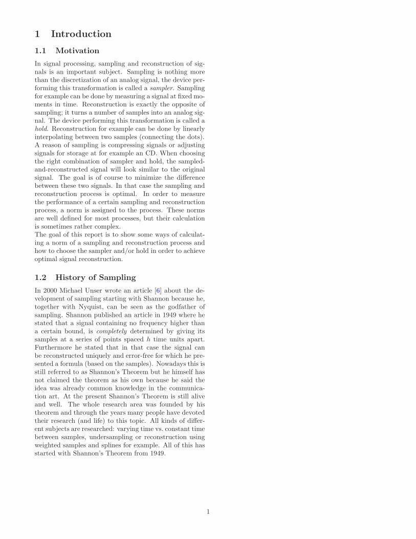
In signal processing, sampling and reconstruction of sig-nals is an important subject. Sampling is nothing morethan the discretization of an analog signal, the device per-forming this transformation is called a sampler. Samplingfor example can be done by measuring a signal at fixed mo-ments in time. Reconstruction is exactly the opposite ofsampling; it turns a number of samples into an analog sig-nal. The device performing this transformation is called ahold. Reconstruction for example can be done by linearlyinterpolating between two samples (connecting the dots).A reason of sampling is compressing signals or adjustingsignals for storage at for example an CD. When choosingthe right combination of sampler and hold, the sampled-and-reconstructed signal will look similar to the originalsignal. The goal is of course to minimize the differencebetween these two signals. In that case the sampling andreconstruction process is optimal. In order to measurethe performance of a certain sampling and reconstructionprocess, a norm is assigned to the process. These normsare well defined for most processes, but their calculationis sometimes rather complex.The goal of this report is to show some ways of calculat-ing a norm of a sampling and reconstruction process andhow to choose the sampler and/or hold in order to achieveoptimal signal reconstruction.
1.2 History of Sampling
In 2000 Michael Unser wrote an article [6] about the de-velopment of sampling starting with Shannon because he,together with Nyquist, can be seen as the godfather ofsampling. Shannon published an article in 1949 where hestated that a signal containing no frequency higher thana certain bound, is completely determined by giving itssamples at a series of points spaced h time units apart.Furthermore he stated that in that case the signal canbe reconstructed uniquely and error-free for which he pre-sented a formula (based on the samples). Nowadays this isstill referred to as Shannon’s Theorem but he himself hasnot claimed the theorem as his own because he said theidea was already common knowledge in the communica-tion art. At the present Shannon’s Theorem is still aliveand well. The whole research area was founded by histheorem and through the years many people have devotedtheir research (and life) to this topic. All kinds of differ-ent subjects are researched: varying time vs. constant timebetween samples, undersampling or reconstruction usingweighted samples and splines for example. All of this hasstarted with Shannon’s Theorem from 1949.
1

2 Background Information
2.1 Introduction
The idea behind sampling is to reduce the data quantityof an (analog) signal or to be able to record the signal in away that allows one to reconstruct the signal afterwards.
Example 2.1.1. In order to record music on a CD, themusic is sampled and these samples are recorded on theCD. When playing the CD, the CD-player reconstructsan analog signal based on the samples recorded on theCD.
The device that turns the analog signal u (in Exam-ple 2.1.1 the music) in discrete samples u is called a sam-pler and it is denoted by the symbol S. The device that re-constructs an analog signal y (in Example 2.1.1 the soundleaving the speakers) from the samples u is called a holdand is denoted by the symbol H. An illustration of thisset-up is shown in Figure 1. Here the device G is calledthe signal generator. In the context of Example 2.1.1 thisgenerator can be seen as the instruments producing themusic.Of special interest is the error signal e which is the differ-ence between the original signal u and the sampled-and-reconstructed signal y. The smaller this signal e, the morethe reconstructed signal looks like to the original signal.
we
u uy
u
+
−H S
G
Figure 1: A system with sampler S, hold H, gen-erator G, generator signal w, input signal u, sam-pled input signal u, output signaly and error sig-nal e
In general a continuous time signal is represented by anordinary letter and round brackets, e.g. u(t). Whereas therepresentation of a sampled (discrete) signal is a barredletter and square brackets, e.g. u[j].
2.1.1 Sampler
The reason for sampling and reconstruction of a signal isstated above. This subsection will focus on some proper-ties of samplers. A sampler turns an analog input signalu(t) into a discrete signal u[j], see Figure 2.
For a sampler the time between two consecutive samplesis called the sampling period. This sampling period canbe uniform (constant) or it can vary over time. For someapplications it is desirable to use a varying sampling timewhereas in this report the sampling period will be uniform
S
u[j] u(t)
h
Figure 2: Example of a sampler that takes sam-ples according to the value of the input functionat multiples of the sampling period h (the idealsampler)
and it is denoted byh.
Besides a uniform sampling period, the samplers S in thisreport are assumed to be Linear Discrete Time Invariant(LDTI), see Definition A.1.8. This means that it is linearand that a shift of the analog input by a multiple k ofthe sampling period h results in a shift of the sampled(discrete) output by k samples
Sσkh = σkS.
It can be shown [3] that essentially every LDTI samplercan be written as a convolution
u = Su : u [j] =
∫ ∞
−∞
ψ(jh− s)u(s)ds, j ∈ Z (2.1)
for some function ψ(t). This function ψ(t) is called thesampling function and it defines the sampler, see Defi-nition A.2.2. The most conventional sampler is the idealsampler which can be obtained by taking ψ(t) as the Diracdelta function δ(t). This results in samples that are justthe values of the input at multiples of the sampling period,see Figure 2. Of course the class of samplers (2.1) is muchricher than the ideal sampler. For instance, taking
0 h
1h
ψ(t) = 1h1[0,h](t) =
leads to samples that are averages of the input over onesampling period.Clearly, sampling throws away an enormous amount ofinformation since, based purely on the samples one can-not determine a unique analog input signal. Therefore,in order to reconstruct the original analog input signalto a certain extend, one must assume certain propertiesof the input signal. For example, if the (ideal) samplesu[j] := u(jh) are all zero, the input signal might have beenthe zero signal u(t) = 0. But it might also have been thesignal
u(t) = sin(π
ht)
which has its zeros in multiples of h. This shows that it isnot clear what the input signal has been considering only
2

the information of the samples. For example, informationabout the frequency of the signal can be used in order toreconstruct the signal to a certain extend.The famous result of Shannon (see Theorem A.2.4) showsthat if the maximal frequency of the analog input signalu(t) is bounded by the Nyquist frequency ωnyq, defined as
ωnyq :=π
h
(see Definition A.2.1), then the signal can be constructeduniquely and error-free. Note that this is an assumptionon the input signal. The ideal sampler
ψ(t) = δ(t).
in combination with the correct hold, which will be men-tioned shortly in Subsection 2.1.2, will achieve this error-free reconstruction.
2.1.2 Hold
In this subsection some properties of holds will be re-viewed. A hold turns a discrete signal u[j] into an analogoutput signal y(t), see Figure 3.
H
y(t) u[j]
Figure 3: Example of a hold that holds the out-put constant over one sampling period (zero-order hold)
The holds H in this report are assumed to be LDTI devicesas are the samplers. In this case this means that it is linearand that a shift of the discrete input by k samples results ina shift of the reconstructed (analog) output by a multiplek of the sampling period h
Hσk = σkhH.
Similar to the sampler it can be shown [3] that essentiallyevery LDTI hold can be written as a convolution
y = Hu : y(t) =∑
j∈Z
φ(t− jh)u [j] , t ∈ R (2.2)
for some function φ(t). This function φ(t) is called thehold function and it defines the hold, see Definition A.2.3.Just like for the sampler, the class of holds (2.2) is a richclass containing numerous holds. For example the zero-order hold which keeps the analog output signal constantover each sampling period can be obtained by using thehold function
0 h
1
φ(t) = 1[0,h](t) =
A schematic representation of this hold is shown inFigure 3. Another example of a hold is the one thatlinearly interpolates between consecutive samples. Thishold is defined by the hold function
0 h−h
1
φ(t) =(
1 − |t|h
) 1[−h,h](t) =
and is illustrated in Figure 4.
H
y(t) u[j]
Figure 4: Example of a hold that linearly inter-polates between two consecutive samples (first-order hold)
From these two examples one can see that the quality ofthe analog output can vary a lot using different holds.The zero-order hold only uses the information from onesample, whereas the first-order hold also uses the infor-mation from the neighboring samples. As mentioned inSubsection 2.1.1 Shannon’s theorem (Theorem A.2.4) alsoprovides the hold function that will reconstruct a signalerror-free and uniquely if the maximum frequency of thesignal is smaller than ωnyq. Shannon’s reconstruction for-mula reads
f(t) =∑
k∈Z
sinc (t− kh) f(kh).
Hence the hold function defining this hold (referred to asthe sinc-hold) is the sinc:
sinc (t) :=sin(πt)
πt.
So by Shannon’s theorem using the ideal sampler and thesinc-hold leads to an error-free reconstruction of the analoginput signal if the maximal frequency of the input signalis smaller than ωnyq. And thus as explained previouslyShannon’s sampler and hold are defined by the functions
ψ(t) = δ(t) (2.3)
φ(t) = sinc (t) . (2.4)
3

2.1.3 Sampler and Hold combination
The combination of sampler and hold sometimes has thespecial property of being Linear Continuous Time Invari-ant (LCTI), see Definition A.1.7, and this has some usefulconsequences.In general both sampler and hold are LDTI whichmeans that they have certain shift-properties (see Subsec-tions 2.1.1 and 2.1.2). In addition if a device is LCTI, theproperties are somewhat extended. Sometimes the com-bination of sampler and hold HS is LCTI whereas bothsampler and hold individually are not. If the combinationHS is LCTI, then by definition it is linear and a shift ofthe analog input by any real number τ results in a shift ofthe analog output by τ
(HS)στ = στ (HS).
Since systems that are not LCTI have no classic transferfunction (see Subsection 2.3) the individual transfer func-tions of H and S mostly do not exist (only in the specialcase that both H and S are LCTI and stable, see Sub-section 2.3). Sometimes the combination HS does have atransfer function. In order to avoid notational confusion,if HS has a transfer function, its notation is
F (s) := (HS)(s).
In general the combination HS is assumed to be LDTIand its mapping can be constructed by substituting theexpression for u[j] (2.1) in the expression for y(t) (2.2).This results in a mapping from the input u to the out-put y = HSu
y(t) =∑
j∈Z
φ(t− jh)
∫ ∞
−∞
ψ(jh− s)u(s) ds.
Since the summation is independent of the variable s itcan be taken inside the integral leading to a product ofthe hold- and sampler function
y(t) =
∫ ∞
−∞
∑
j∈Z
φ(t− jh)ψ(jh− s)u(s) ds.
Thus HS is an integral operator of the form
y(t) =
∫ ∞
−∞
κ(t, s)u(s) ds
where κ(t, s) is called the kernel of HS and it equals
κ(t, s) :=∑
j∈Z
φ(t− jh)ψ(jh− s). (2.5)
Note that this kernel h-shift invariant, i.e. for all l ∈ Z
κ(t+ lh, s+ lh) =∑
k∈Z
φ(t + lh− jh)ψ(jh− s− lh)
=∑
k∈Z
φ(t + (l − j)h)ψ((j − l)h− s)
=∑
k∈Z
φ(t − jh)ψ(jh− s)
= κ(t, s).
2.1.4 Signal Generator
The last device from the setting in Figure 1 is the signalgenerator G. This device is assumed to be LCTI (see Defi-nition A.1.7) and is assumed to have a strictly proper andstable transfer function G(s) (see Subsection 2.3). It canbe shown [3] that every LCTI generator G can be writtenas a convolution
u = Gw : u(t) =
∫ ∞
−∞
g(t− τ)w(τ) dτ, k ∈ Z
for some function g(t). This function g(t) is called theimpulse response and it defines the generator.In this report the symbol G will also be used as the symbolfor a general (not explicitly specified) system. From thecontext it will be clear when G refers to a signal generatorand when to a general system.It can be shown [3] that a general LDTI system y = Gu isof the form
y(t) =
∫ ∞
−∞
g(t, s)u(s) ds
where g(t, s) is called the kernel and it is h-shift invariant:
g(t+ h, s+ h) = g(t, s).
2.2 Signals
This subsection will focus on the representation of signalsand some of their properties. Furthermore a way of rep-resenting a continuous-time signal as a kind of discretesignal (Lifting) is mentioned.
2.2.1 Laplace transform
In signal processing the most straight forward way to rep-resent a signal f is the time domain representation, i.e.
f(t), ∀t ∈ R.
However for some applications it is convenient to knowthe Laplace transform of a signal. The Laplace transformF (s) of a signal f(t) is defined as
F (s) :=
∫ ∞
−∞
f(t)e−st dt (2.6)
for those s ∈ C for which this integral exists. This trans-formation is called the two-sided Laplace transform be-cause the signal is integrated from −∞ to ∞. The one-sided Laplace transform is defined as well
F1(s) :=
∫ ∞
0
f(t)e−st dt
for those s ∈ C for which this integral exists. Clearly thisone-sided Laplace transform throws away a lot of infor-mation about the signal if the signal is non-causal (seeDefinition A.1.9). A signal f(t) is said to be causal if
f(t) = 0 ∀t < 0.
4

This report will consider non-causal signals as well, there-fore the two-sided Laplace transform will be used. So fromnow on the two-sided Laplace transform (2.6) will be re-ferred to as the Laplace transform.
2.2.2 Fourier transform
It can be shown [1] that for an absolutely integrable signalf(t), i.e.
∫ ∞
−∞
|f(t)| dt <∞
the Laplace transform (2.6) exists for all s ∈ C withRe (s) = 0. This means that the Laplace transform existson the entire imaginary axis. Write the complex numbers as σ + iω with σ and ω real numbers and i being theimaginary unit
√−1. Now the Laplace transform looks
like
F (σ + iω) =
∫ ∞
−∞
f(t)e−σt−iωt dt
=
∫ ∞
−∞
f(t)e−σte−iωt dt
for σ = 0 which leads to
F (iω) =
∫ ∞
−∞
f(t)e−iωt dt. (2.7)
where ω is the frequency in radians per time unit. Thistransform exists for all ω ∈ R and is a special case of theLaplace transform, it is called the Fourier transform. TheFourier transform has an inverse given by
f(t) =1
2π
∫ ∞
−∞
F (iω)eiωt dω. (2.8)
In this report, the Fourier transform F (iω) of a signalf(t) is always denoted by a capital. Using Equations (2.7)and (2.8) one can switch between the time domain rep-resentation and the frequency domain representation of asignal.If a signal f(t) is square integrable, i.e. the energy of thesignal Ef is finite
Ef :=
∫ ∞
−∞
|f(t)|2 dt <∞
then the two representations have a special property cap-tured in Parseval’s theorem (see Theorem A.3.6). Thistheorem shows that integrating the signal over all timeequals integrating the signal over all frequencies, exceptfor a contstant
∫ ∞
−∞
|f(t)|2 dt =1
2π
∫ ∞
−∞
|F (iω)|2 dω. (2.9)
This means that the energy of the signal equals the energyof its Fourier transform, except for the constant 2π.
2.2.3 Lifting
Lifting is a technique to represent a continuous time signalf(t) with t ∈ R on a smaller, finite time interval [0, h). Infact the signal is cut into an infinite number of intervals,each of length h, see Definition A.4.1. However this meansthat the lifted signal f now is a function of two variables,i.e. k and τ , and it is defined as
f [k](τ) = f(kh+ τ) k ∈ Z, τ ∈ [0, h).
In other words, with lifting, a signal f on R is consideredas a sequence of functions on the interval [0, h). A positiveaspect of this process is that there is no loss of information.The process of lifting is illustrated in Figure 5. The idea
−2h −h 0 h 2h t→
f(t) in continuous time
0 h 0 h 0 h 0 h
−2 −1 0 1 k →
f [k] in the lifted domain
Figure 5: Lifting the analog signal f(t) = 1 +cos( π
2h t)
behind this representation is to allow only time shifts thatare multiples of h. This implies that if a continuous-timesystem y = Gu (see Subsection 2.3) is h-periodic, then inlifted representation u = Gy is shift invariant (i.e. a shiftin k) [3].It turns out [3] that the Fourier transform of a lifted signal
f exists if the Fourier transform of f itself exists, and it isgiven by
Ff = f(eiωh; τ) :=∑
k∈Z
f [k] (τ)e−iωkh
where the frequency ω is 2π-periodic, see Definition A.4.2.A very useful result [3] is a theorem that shows thatthere exists a bijection from the lifted fourier transformf(eiωh; τ) and the classical Fourier transform F (iω), seeTheorem A.4.3. The projection in one direction is givenby
f(eiωh; τ) =1
h
∑
k∈Z
F (iωk)eiωkτ (2.10)
for all τ ∈ [0, h), where ωk = ω+2ωnyqk is the kth aliasedfrequency (see Definition A.2.1). And its inverse is givenby
F (iωk) =
∫ h
0
f(eiωh; τ)e−iωkτdτ.
This allows to switch between the classical representationof a signal and its lifted representation using both (theordinary and the lifted) Fourier transforms.
5

2.3 Systems
This subsection reviews mathematical systems, their prop-erties and why it is convenient to use systems in signalreconstruction.In general a mathematical input-output system is a devicethat receives an input signal u and produces a output sig-nal y based on this input signal. Figure 6 shows a graph-ical interpretation of an input-output system. Examplesof such systems are samplers, holds and signal generators.In general the input- and output signals of a system aremultidimensional. This means that the system is multiinput multi output (MIMO). In order to understand theresults derived in this report, using MIMO systems is sim-ply unnecessarily complicated. Therefore this report willfocus on systems that are single input single output (SISO)only, but all results can be extended to MIMO systems byuse of matrix operations.
u yG
Figure 6: A system G with input u, output y
If a system G is LCTI (see Definition A.1.7), then thereexists a convolution (see Definition A.1.10) that obtainsan output y based on the input u
y(t) = (g ∗ u)(t) =
∫ ∞
−∞
g(t− τ)u(τ) dτ. (2.11)
The function g(t) describes the system.A system G is said to be BIBO-stable (see Definition A.1.2)if the output is bounded for every bounded input. G isBIBO-stable iff the infinite integral of |g(t)| is finite:
∫ ∞
−∞
|g(t)| dt <∞
and then the (two sided) Laplace transform of the functiong(t) exists as well on the imaginary axis. If additionallythe in- and output have Laplace transforms, the systemcan be written as
Y (s) = G(s)U(s)
often notated as simply
y = G(s)u.
Note that this transfer function can only exist if the sys-tem is LCTI, if the system is only LDTI it has no classictransfer function. In general the in- and output signalscan be multidimensional which results in a transfer ma-trix. The dimensions of the in- and output signals aredenoted by nu and ny respectively. In this report nu andny are both one.
If the transfer function G(s) is rational and proper thetransfer function can be written in the form
G(s) = C(sI −A)−1B +D (2.12)
with real matrices A, B, C and D. A rational transferfunction is said to be proper if the degree of the numer-ator does not exceed the degree of the denominator. Ifadditionally the transfer function is strictly proper (thedegree of the numerator is smaller than the degree of thedenominator), then D equals zero.Furthermore, if the system (2.12) is considered causal andproper, then the impulse response g(t) of (2.12) is
g(t) = CeAtB · 1(t) +Dδ(t). (2.13)
This corresponds to a state space representation
x = Ax +Buy = Cx+Du
(2.14)
with a new variable x: the internal state of the system.Figure 7 shows a block-diagram of a proper state spacerepresentation.
ux x
yB1s C
A
D
+ +
Figure 7: The state space respresentation of sys-tem (2.14) with input u, output y, real matricesA, B, C and D and where 1
s denotes a pure in-tegrator
A common notation for the state space representation ofa transfer function is
G(s) = C(sI−A)−1B+Ds=
[
A BC D
]
⇔
x = Ax+Buy = Cx+Du.
Equations (2.11) and (2.13) combined provide the solutionfor the output y
y(t) =
∫ ∞
−∞
g(t− τ)u(τ) dτ
=
∫ ∞
−∞
(
CeA(t−τ)B · 1(t− τ) +Dδ(t− τ))
u(τ) dτ
=
∫ t
−∞
CeA(t−τ)Bu(τ) dτ +Du(t).
So, to conclude this subsection, if an LCTI system G isstable it has a transfer function G(s) for Re (s) = 0. Ifadditionally the system is causal and the transfer functionis rational and proper, then the system has a state spacerepresentation of the form (2.14).This report will focus on strictly proper systems, i.e. ma-trix D is the zero matrix.
6

2.4 Norms
In order to decide which of two sampler-and-hold combi-nations is the best one, some kind of measure will be usedto compare multiple options. Such a measure is calleda norm, see Definition A.3.1. This subsection will showsome examples and applications of norms. Of special inter-est are the norms suitable for signals and systems. Somephysical interpretations are mentioned as well.In general, a norm (denoted by ||·||) is measure on a vectorspace that assigns a non-negative number to every elementof the space. This number is the size of the element, mea-sured by this specific norm. One vector space can havemultiple norms with different (physical) interpretations.
Example 2.4.1. In the vector space R3 every elementx ∈ R3 is of the form
x =
x1
x2
x3
. (2.15)
The Euclidean norm on R3
||x||2 =√
x21 + x2
2 + x23
represents the distance of the element x to the origin.Whereas the norm
||x||∞ = maxx1, x2, x3
represents the maximum distance in one direction (x1-, x2-or x3-axis) of the element x to the origin. Both ||·||2 and||·||∞ are norms on the space R3 but they have differentinterpretations.
Example 2.4.1 shows that there exist several norms forone vector space. The norm that is most convenient forsignals is studied in Subsection 2.4.1. For a system it isnot straight forward how to compute its norm, Subsec-tion 2.4.2 will show the solution to this problem.
2.4.1 Signal Norms
For signals it is convenient to work with a norm thatrepresents the energy of the signal. Before introducingthis norm, first the vector space on which the signals liveneeds to be introduced. In this report this is the spaceL2(R) see Definition A.3.3. The space L2[a, b] consists ofall (Lebesque-integrable) functions f(t) with finite energyon the interval [a, b]:
∫ b
a
|f(t)|2 dt <∞.
For all elements f(t) in the space L2[a, b] the norm
||f ||L2 :=
√
∫ b
a
|f(t)|2 dt
represents the square root of the signal’s energy. Note thatL2(R) is besides a normed space an inner product spaceas well (see Definition A.3.2). The inner product betweentwo elements in L2(R) is defined as
〈f, g〉 :=
∫ ∞
−∞
f(t)g(t) dt.
By definition of the inner product, two elements are or-thogonal if their inner product equals zero. Furthermore,the relation between the inner product and the norm of asignal is the following: the norm of a signal is the squareroot of the inner product of the signal with itself
||f ||L2 =√
〈f, f〉.
2.4.2 LCTI System Norms
As mentioned in the introduction of this subsection, it isslightly more complicated to calculate norms of a system.However, if a system G is stable and LCTI the norm ofthe system can be defined in a similar way as the signalnorms. Recall that if G is stable and LCTI the system hasa transfer function G(s) mapping the input on the output.Define yδ as the response of the system to the Dirac deltafunction
yδ := Gδ.
If a system is stable and LCTI, the L2 system norm is theL2 signal norm of the system’s response to the Dirac deltafunction
||G||L2 := ||yδ||L2 =
√
∫ ∞
−∞
|Gδ(t)|2 dt (2.16)
=
√
∫ ∞
−∞
|(g ∗ δ)(t)|2 dt
=
√
∫ ∞
−∞
∣
∣
∣
∣
∫ ∞
−∞
g(t− τ)δ(τ) dτ
∣
∣
∣
∣
2
dt
=
√
∫ ∞
−∞
|g(t)|2 dt
= ||g||L2 .
Note that ||G||L2 is a system norm whereas ||yδ||L2 and||g||L2 are signal norms. Furthermore, the L2-norm forsystems has an interpretation in terms of stochastic sig-nals. If the input signal is white noise (see Defini-
tion A.1.11), then the squared norm of the system ||G||2L2
is exactly the variance or power of the output.Equation (2.16) is the definition of the L2-norm for sys-tems but it is not straightforward how to calculate thisnorm. The following equation shows how to compute the
7

system norm in the frequency domain
||G||L2 = ||yδ||L2 =
√
∫ ∞
−∞
|Gδ(t)|2 dt
=
√
∫ ∞
−∞
|(g ∗ δ)(t)|2 dt
=
√
1
2π
∫ ∞
−∞
|G(iω) · 1|2 dω
=
√
1
π
∫ ∞
0
|G(iω)|2 dω (2.17)
where G(iω) is the transfer function G(s) evaluated in thepurely imaginary points iω. The function G(iω) is theFourier transform of the impulse response g(t). Note that|G(iω)| is an even function and that the derivations aboveonly hold for LCTI systems.In order to calculate |G(iω)|2 the conjugate of a real trans-fer matric G∼(s), defined as
G∼(s) := [G(−s)]T (2.18)
will be used. Similar to the scalar case, the squared abso-lute value of a multidimensional real transfer function isthe function itself times its conjugate
|G(iω)|2 = G∼(iω)G(iω).
This leads to the following expression for the L2 systemnorm of an LCTI system G:
||G||L2 =
√
1
π
∫ ∞
0
G∼(iω)G(iω) dω. (2.19)
This is the expression for the L2 system norm for anLCTI system that will be used in further sections of thisreport.
2.4.3 LDTI System Norms
The L2 system norm of an LDTI system G is defined as
||G||L2 :=
√
1
h
∫ h
0
||Gδ(· − t)||2L2 dt (2.20)
which can be seen as the integral over the response of thesystem to a series of Dirac delta functions. There does notexist a nice expression for this norm that is easy to workwith yet.
2.5 Calculation of the L2 system norm
An expression for the L2 norm for a system was derived inSubsection 2.4.2 and given by (2.19), still this expressionis not solvable in a clear way. This subsection will providean explicit solution for the L2 system norm and it containsa few examples to show how this norm is calculated.
2.5.1 Classical Calculation
If the matrix A of the transfer function
G(s) = C(sI −A)−1B
is stable (see Definition A.3.8) the L2 system norm ofG (2.19) can be calculated in a classic way [5]. A Ma-trix A is stable if all its eigenvalues λi lie in the open lefthalf of the complex plane C:
Re (λi) < 0 ∀i.
If so, the system has a unique solution P of the Lyapunovequation [5]:
ATP + PA = −CTC. (2.21)
It is a classic result that if A is stable, then the calculationof the L2 system norm of G can be reduced to
||G||L2 =√BTPB. (2.22)
Example 2.5.1. Consider the system G with transferfunction
G(s) =1
1 + s.
This corresponds to a state space representation
x = −1x+ 1uy = 1x
and the squared magnitude of G(iω) looks like
0 w →
1∣
∣
11+iω
∣
∣
2=
Note that all matrices are only scalars and that thereforeAhas only one eigenvalue, i.e. −1 and thus A is stable. TheLyapunov equation reduces to a simple, scalar equation
−P − P = −1
which has the solution P = 12 . So the L2 system
norm (2.22) equals
||G||L2 =
√
1 · 1
2· 1
=
√
1
2. (2.23)
8

2.5.2 Alternative Calculation
From Subsection 2.3 it is known that a real, rational andstrictly proper transfer function G(s) can be written inthe form
G(s) = C(sI −A)−1Bs=
[
A BC 0
]
.
In combination with (2.18) this gives an expression for theconjugate G∼(s) of the transfer matrix
G∼(s) =[
C(−sI −A)−1B]T
= BT[
(−sI −A)T]−1
CT
= −BT (sI +AT )−1CT .
In Equation (2.19) the transfer function G(s) and its con-jugate G∼(s) form a coupled system G∼G which meansthat the output y of G is the input for G∼. Define K asthis coupled system
K(s) := G∼(s)G(s).
K also has a state space representation which will beshown next [5]. Say, G has input u, output y and state xwhereas G∼ has input y, output z and state q, then thecoupled system can be written as
y = G(s)u
z = G∼(s)y
z = G∼(s)G(s)u
z = K(s)u.
Since both transfer functions G and G∼ are real, rationaland strictly proper, they both have a state space realiza-tion
y = G(s)u ⇔
x(t) = Ax(t) +Bu(t)y(t) = Cx(t)
z = G∼(s)y ⇔
q(t) = −AT q(t) − CT y(t)z(t) = BT q(t).
Combining these two state space realizations and mergingthem into one vector notation leads to
x
q
z
=
A 0 B
−CTC −AT 0
0 BT 0
x
q
u
which is the state space representation of K(s). Definethe real matrices A, B and C as
[
A B
C 0
]
:=
A 0 B
−CTC −AT 0
0 BT 0
. (2.24)
This means that K(s) can be written as
K(s) = C(sI − A)−1B.
Now, the L2 system norm (2.19) reduces to the integralover K(s) for which a state space representation exists.Note that CB = 0. It can be shown [5] that if A, B andC are real matrices and if CB = 0, then the semi-infiniteintegral of K(s) can be determined explicitly:
∫ ∞
0
K(iω) dω = iC log(
iA)
B. (2.25)
This equation only holds as long as A has no eigenvaluesλi on the imaginary axis:
Re (λi) 6= 0 ∀i.
Note that this does not mean that A has to be stable (seeDefinition A.3.8); A can have eigenvalues in the entirecomplex plane as long as they do not lie on the imaginaryaxis.Equation (2.25) uses the principal logarithm (see Defini-tion A.3.7) of a matrix. MATLAB R© has a command thatgenerates the principal logarithm for any square matrix ofwhich the real eigenvalues are strictly positive.Equation (2.25) provides that the L2 system norm of asystem G can be written as
||G||L2 =
√
i
π
[
C log(
iA)
B]
(2.26)
provided that A has no eigenvalues on the imaginary axes.
Example 2.5.2. Consider the same system G as in Ex-ample 2.5.1
G(s) =1
1 + s
s=
[
−1 11 0
]
.
This example will show how to calculate the L2 systemnorm of this system in the way explained in Subsec-tion 2.5.2
In order to calculate the L2 system norm, first A, B andC are computed:
A =
[
−1 0−1 1
]
B =
[
10
]
C =[
0 1]
Note that the eigenvalues of A are −1 and 1, so Equa-tion (2.26) can be applied to this system. The principallogarithm of iA is computed using MATLAB R©:
log(
iA)
=
[
−π2 i 0
−π2 i π
2 i
]
.
Now Equation (2.26) can be exploited to determine the L2
9

norm of the system G(s) = 11+s
||G||L2 =
√
i
π
(
[
0 1]
[
−π2 i 0
−π2 i π
2 i
] [
10
])
=
√
− i
π· πi
2
=
√
1
2. (2.27)
Of course, the L2 norm of this system can also be de-termined analytically in order to verify the validation ofEquation (2.26). To do this, Equation (2.17) will be ex-ploited together with the conjugate
G∼(s) =1
1 − s
of the transfer function G(s). The squared magnitude ofthe transfer function reads (see Equation (2.18))
|G(iω)|2 =1
1 + iω· 1
1 − iω
=1
1 + ω2.
Now the L2 norm of the system G can be calculated ana-lytically
||G||L2 =
√
1
π
∫ ∞
0
|G(iω)|2 dω
=
√
1
π
∫ ∞
0
1
1 + ω2dω
=
√
1
πlim
ω→∞arctan(ω)
=
√
1
π· π2
=
√
1
2.
Note that this norm is exactly the same as the one cal-culated using the principal logarithm (2.27) and the onecalculated using the classical expression (2.23).
In Example 2.5.2 the transfer function is SISO thereforeit is rather easy to calculate the L2 system norm analyt-ically. Whereas calculating the norm using the principallogarithm is a more complex calculation. In general, if thetransfer function is MIMO it is a lot more complicated tocalculate the norm analytically. Therefore it is very con-venient to work with Equation (2.22) or (2.26) in order tocalculate the L2 norm of a system.
10

3 Truncated System Norm
3.1 Introduction
The signal- and system norms on the vector space L2
are introduced in Subsections 2.4.1 and 2.4.2 respectively.This subsection will focus on the concept of frequencytruncated system norms. Figure 1 on page 2 shows theset up for a sample-and-reconstruction problem, this sys-tem will be referred to as the error system. The signal wis the input signal for G that will generate the signal to besampled and reconstructed u. The mapping from w to ereads
e = (I −HS)Gw.The goal is, given a (fixed) sampling period h, to minimizethe error e in some sense. For instance that the mappingfrom w to e is minimized according to the L2 system norm:
minH,S
||(I −HS)G||L2 . (3.1)
Here the norm is minimized over all stable and LDTI sam-plers and holds. The interpretations of equation (3.1)reads that the smaller the norm the more the sampled-and-reconstructed signal y looks like the original signal u.It can be shown [5] that if G is LCTI, then the combina-tion of sampler and hold that minimizes the norm (3.1)is in fact LCTI and stable as well. This means that thecombination F = HS has a transfer function (see Subsec-tion 2.1.3):
F (s).
3.2 Monotonically decreasing response
If additionally the system G has a monotonically decreas-ing magnitude |G(iω)| for positive ω, then the combinationof sampler and hold is the ideal low pass filter:
0 ωnyq
1
ω →F (iω) = 1[−ωnyq,ωnyq](ω) =
This low-pass filter can be achieved using a low pass fil-ter in combination with the ideal sampler and sinc-holdfrom Shannon’s Theorem, see Equations (2.3) and (2.4)on page 3.The system (I −HS) with the minimizing sampler andhold is in fact an ideal high-pass filter feeding through allfrequencies higher than the Nyquist frequency ωnyq.So for a fixed sampling period h and an LTCI systemG with monotonically decreasing magnitude |G(iω)|2, thebest one can do is filter out the first Nyquist band N1
consisting of the frequencies [0, ωnyq), from the frequencyresponse (see Definition A.2.1).Now the question arrises what the L2 norm of the system(I −HS)G with optimal sampler-and-hold combination is.This is in fact the object that was minimized in the first
place, see Equation (3.1). The norm of the error systemcan be calculated in the same way as in Subsection 2.5.Now the optimal sampler-and-hold combination causes themagnitude |(I − F (iω))G(iω)|2 of the whole system to beof the form
|(I − F (iω))G(iω)|2 =
0 0 < ω ≤ ωnyq
|G(iω)|2 ω > ωnyq
since (I − F )(iω) is a high-pass filter. This leads to thefollowing expression of the system norm
||(I −HS)G||L2 =
√
1
π
∫ ∞
0
|(I − F (iω))G(iω)|2 dω
=
√
1
π
∫ ∞
ωnyq
|G(iω)|2 dω. (3.2)
Equation (3.2) is called the truncated L2 system norm ofthe system G and is denoted by
||G||ωnyq:=
√
1
π
∫ ∞
ωnyq
|G(iω)|2 dω. (3.3)
Note that Equation (3.3) is in fact not really a norm (seeDefinition A.3.1) since ||G||ωnyq
= 0 does not necessarily
imply G(iω) = 0 for all ω ∈ [0,∞].
3.2.1 Unstable matrix A
The truncated L2 system norm (3.3) is almost the sameas the L2 system norm (2.17) on page 8 except that theintegral of the truncated L2 system norm (3.3) starts atthe Nyquist frequency instead of at zero. It turns out thatthe truncated L2 system norm (3.3) can be calculated in asimilar way as the oridinary L2 system norm (2.17) usingthe state space representation
K(s) = C(sI + A)−1B
as defined in Subsection 2.5. Now the truncated L2 systemof G can be expressed in terms of the real matrices A, Band C
||G||ωnyq=
√
1
π
∫ ∞
ωnyq
|G(iω)|2 dω
=
√
1
π
∫ ∞
ωnyq
G∼(iω)G(iω) dω
=
√
1
π
∫ ∞
ωnyq
K(iω) dω.
This is the same derivation as used for Equation (2.17). Itcan be shown [5] that the semi-infinite integral of K(iω)also exists if the lower bound of the integral is larger thanzero:
∫ ∞
ωnyq
K(iω) dω = iC log(
ωnyqI + iA)
B
11

provided that ωnyq > ωmax := max |ωk|, where the maxi-
mum is taken over all pure imaginary eigenvalues iωk of A.This leaves a concrete expression for the truncated systemnorm
||G||ωnyq=
√
i
π
[
C log(
ωnyqI + iA)
B]
(3.4)
which can be used to calculate the truncated L2 systemnorm explicitly. So if the sampler-and-hold combinationis optimal, the L2 norm of the error system reduces to
||(I −HS)G||L2 =
√
i
π
[
C log(
ωnyqI + iA)
B]
. (3.5)
Example 3.2.1. Consider the same system G as in Ex-ample 2.5.1 with the transfer function
G(s) =1
1 + s
and sampling period h = 1. The squared magnitude ofthe transfer function looks like
0 w →
1
|G(iω)|2 =
Since the magnitude of G is monotonically decreasing, theoptimal hold-and-sampler combination will cut of the firstNyquist band:
0 w →
1
ωnyq
|(I − F (iω))G(iω)|2 =
The matrices A, B and C are the same as in Example 2.5.2which leads to the calculation of the truncated L2 systemnorm using Equation (3.5). In this case the Nyquist fre-quency ωnyq = π
h equals π
||G||ωnyq=
√
i
π
(
[
0 1]
log
([
π − i 0−i π + i
])[
10
])
=
√
i
π· −0.3082i
= 0.3132.
Again, the norm can be determined analytically. Exam-ple 2.5.2 already derived the anti-derivative of the inte-
grant
||G||ωnyq=
√
1
π
∫ ∞
π
1
ω2 + 1dω
=
√
1
π
(
limω→∞
arctan(ω) − arctan(π))
=
√
1
π
(π
2− 1.2626
)
= 0.3132.
Note that this norm, which is calculated analytically, isexactly the same as the on calculated using the principlelogarithm.In order to get an indication how much energy of the origi-nal system G is preserved by sampling and reconstruction,the following formula is exploited
||G||2L2 − ||(I −HS)G||2L2
||G||2L2
× 100% =0.5 − 0.0981
0.5× 100%
= 80.4%.
In this formula the numerator is the energy of the systemitself minus the energy of the error system. So the nu-merator consists of thet total energy that is preserved bysampling and reconstruction. Dividing this by the energyof the system and multiplying by 100 gives the percentageof energy that is preserved.So 80.4% of the system’s energy is preserved by samplingand reconstruction if a sampling period h = 1 is used incombination with the optimal sampler and hold combina-tion.
3.2.2 Stable matrix A
Subsection 3.2.1 showed how to calculate the norm
||(I −HS)G||L2 (3.6)
of the error system for the optimal sampler-and-hold com-bination
F (iω) = 1[−ωnyq,ωnyq](ω). (3.7)
The system G is assumed to be LCTI and to have a mono-tonically decreasing magnitude |G(iω)|2, and the samplingperiod, h, is fixed.In this case the L2 norm of the optimal error system(I −HS)G reduces to the truncated L2 system norm ofonly G as shown in Subsection 3.2
||(I −HS)G||L2 = ||G||ωnyq
=
√
i
π
[
C log(
ωnyqI + iA)
B]
.
However, calculating A, B and C requires a lot of thecomputational capacity since the dimensions of A are twiceas large as of A itself. The computational burden can bereduced if the matrix A of the transfer function
G(s) = C(sI −A)−1B
12

is stable. Subsection 2.5.1 showed that if A is stable theL2 system norm of G reduces to
||G||L2 =√BTPB.
It can be shown [5] that if G is stable, strictlyproper and if G has the state space representationG(s) = C(sI −A)−1B with real matrices A, B and C andA is stable, then
||G||ωnyq=
√
− 2
πIm (BTP log (ωnyqI + iA)B)
=
√
||G||2L2 −2
πIm (BTP log (iωnyqI − iA)B)
where P is the unique solution of the Lyapunov equa-tion (2.21) on page 8. This provides the possibility tocalculate the L2 norm of the error system (3.6) with theoptimal sampler-and-hold combination (3.7), without thecomputational burden of A, B and C.So if the matrix A is stable and the sampler-and-hold com-bination is optimal, the L2 norm of the error system re-duces to
||(I −HS)G||L2 =
√
− 2
πIm (BTP log (ωnyqI + iA)B).
(3.8)
Example 3.2.2. This example will show how to calculatethe truncated L2 system norm using the Equation (3.8).Consider the same system G as in Example 2.5.1 with thetransfer function
G(s) =1
1 + s
and sampling period h = 1. The cut-off frequency ωnyq isagain π. Matrix P is again 1
2 just as in Example 2.5.1 andthus the truncated L2 system norm reduces to
||G||ωnyq=
√
− 2
πIm
(
1 · 1
2· log (π − i) · 1
)
=
√
− 2
πIm
(
1
2· (1.1930− 0.3082i)
)
=
√
− 2
π(−0.154)
= 0.3132.
Note that this norm is the same as the one from Exam-ple 3.2.1.
3.3 Folding
This subsection will discuss how the optimal sampler andhold combination HS will look when the squared magni-tude |G(iω)|2 of the system G is not monotonically de-creasing. Still the goal is to minimize
||(I −HS)G||L2
−3ωnyq −2ωnyq −ωnyq 0 ωnyq 2ωnyq 3ωnyqω →
|G(iω)|2
0 ωnyq 2ωnyq 3ωnyqω →
|G(iω)|2
0 ωnyq
0 ωnyq
Figure 8: Folding the response of |G(iω)|2
over all stable and LDTI samplers and holds.The assumption that G is strictly proper still holds, soeventually there will be a frequency from where on |G(iω)|2will be monotonically decreasing. This frequency is de-noted by
ω∗.
It can be shown [4] that the optimal combination HS fil-ters a finite number of frequency bands out of the response|G(iω)|2. Though the total length of these frequency bandsequals the length of one Nyquist Band: ωnyq. So the pos-sibilities of reducing the L2 system norm are limited byωnyq and thus by h. The next thing is to find the fre-quency bands that need to be filtered out, in order to
13

achieve a minimal L2 norm of the error system. It turnsout that to find these frequency bands, one must fold theresponse |G(iω)|2 like a harmonica. The response is foldedin multiples of the Nyquist frequency and since |G(iω)|2 isan even function, this only needs to be done for positivefrequencies. This process is illustrated in Figure 8.Once the response has been folded, the maximum over thefolded part is determined. In Figure 8 this is just the firstNyquist band N1 because the response is monotonicallydecreasing, but in general the maximum will consist ofseveral small frequency bands each corresponding to an-other Nyquist band Nk. This is the case in Figure 9 andExample 3.3.1.In order to determine the maximum over the folded func-tion, all Nyquist bandsNk will be projected on the interval[0, ωnyq)
hk(ζ) =
|G(i ((k − 1)ωnyq + ζ))|2 k = 1, 3, 5, ...|G(i (kωnyq − ζ))|2 k = 2, 4, 6, ...
with ζ ∈ [0, ωnyq) and k ∈ Z+ the Nyquist band index.Now for every ζ in the domain the maximum over all func-tions hk will be determined numerically
maxk
hk(ζ).
Every folded frequency ζm ∈ [0, ωnyq) has a maximum inone of the Nyquist bands, indicated by the km correspond-ing to this maximum. So the maximum corresponding toζm, lies in the Nyquist band Nkm
. In order to determinethe original frequency corresponding to the maxima, thekm and ζm of every maximum are used to project thefolded frequency back on the original frequency domain(shown in Figure 9)
ωm =
kmωnyq + ζm km = 1, 3, 5, ...kmωnyq + (ωnyq − ζm) km = 2, 4, 6, ...
Folding does not imply that the frequencies with thelargest peak of the response are filtered out, but it fil-ters out the maximum of the folded response.Important for folding is to know from where on the fre-quency response is monotonically decreasing. Here thetransfer matrix K(s) will be exploited once again, recall
|G(s)|2 = G∼(s)G(s) = K(s) = C(sI − A)−1B.
As stated in the beginning of this subsection, the fre-quency response will decrease monotonically after ω∗.This frequency is the largest frequency for which thederivative of K(iω)
d
diωK(iω) = −C(iωI − A)−2B
equals zero. By transferring this expression back to a(MIMO) transfer matrix it is just a matter of equaling the(multiple) numerator(s) to zero. The largest frequency for
−3ωnyq −2ωnyq −ωnyq 0 ωnyq 2ωnyq 3ωnyqω →
|G(iω)|2
0 ωnyq
h1
h2
h3
0 ωnyq 2ωnyq 3ωnyqω →
|G(iω)|2
δ1ǫ1 δ2
|(I − F )G(iω)|2
Figure 9: Unfolding the response of |G(iω)|2 afterdetermining the maxima (red). In blue the fre-quencies that will be filtered in order to achievea minimal L2 norm of the error system. There isone unfiltered band [δ1, ǫ1] and the tail [δn,∞),so in this case n equals 1
which (one of) the numerator(s) equals zero, is ω∗. It isnot difficult to determine in which Nyquist band ω∗ lies.This Nyquist band is called
Nk∗ .
Folding needs to been done up till Nyquist band Nk∗+1
because this band can still tribute to the maximum dueto folding.
14

In the case where |G(iω)|2 is monotonically decreasing, thecalculation of the L2 norm of the error system (3.1) con-sist of only one integral. Since the optimal combinationof sampler-and-hold HS filters several frequency bands ifthe response is not monotonically decreasing, the calcula-tion is somewhat more complicated. The number of fre-quency bands that are filtered out is finite, so the num-ber frequency bands that are unchanged is finite as well(say n). Additionally the ”tail” of the frequency responsecontributes to the norm as well
||(I −HS)G||L2
=
√
√
√
√
1
π
n∑
k=1
∫ ǫk
δk
|G(iω)|2 dω +1
π
∫ ∞
δn+1
|G(iω)|2 dω
=
√
√
√
√
1
π
n∑
k=1
−iC log (Ωk) B + ||G||2δn+1(3.9)
with
Ωk :=(
ǫkI + iA)(
δkI + iA)−1
and A, B and C as defined in (2.24). Furthermore ǫk andδk are respectively the under- and lower bound of the unfil-tered frequency bands. The norm ||G||δn+1
is defined in the
same way as the truncated L2 system norm ||G||ωnyq(3.3),
only with a lower bound δn+1 instead of ωnyq.The optimal sampler-and-hold combination HS now lookslike a series concatenated step functions
F (iω) = 1[0,δ1] +
n∑
k=1
1[ǫk,δk+1]
0
1
F (iω) =
δ1ǫ1 δ2
ǫ2 δn+1ω →
where the following holds for ǫk and δk
(δ1 − 0) +
n∑
k=1
(δk+1 − ǫk) = ωnyq
since the optimal combination HS can only filter multiplefrequency bands with a total length of ωnyq.Note that the above also holds for negative frequenciessince the function F (iω) is an even function.
Example 3.3.1. Consider the ideal sampler, a samplingperiod h = 4 and the system
G(s) =1
(s+ 0.2)2 + 1.
This corresponds to a transfer functionG(s) = C(sI −A)−1B with
A =
[
−0.4 −1.041 0
]
, B =
[
10
]
, C =[
0 1]
.
The squared magnitude of the transfer function looks like
1 ω →
|G(iω)|2 =
The matrix A (as defined in Equation (2.24) on page 9)now looks like
A =
−0.4 −1.04 0 01 0 0 00 0 0.4 −10 −1 1.04 0
which has the eigenvalues −0.2± i and 0.2± i. This meansthat A has no pure imaginary eigenvalues, so the L2 sys-tem norm of G can be calculated using Equation (2.26).
0 0.5 1 1.5 2 2.5 3 3.5 4 4.50
1
2
3
4
5
6
7
Figure 10: Frequency Response of G = 1/((s +0.2)2 + 1). In red the maxima found by foldingand in pink the frequencies that will be filteredout by the optimal hold-and-sampler combina-tion
15

Figure 10 shows the magnitude of the frequency responseof the system G. In this figure, the dotted lines are mul-tiples of the Nyquist frequency ωnyq = π
4 . These are thelines over which the function is folded, similar to Figure 8.After determining the maxima (in red) the function isfolded back (similar to Figure 9) and the frequencies cor-responding to the maxima are highlighted in pink. TheL2 norm of the error system corresponding to the optimalsampler-and-hold combination HS for this specific G canbe calculated using Equation (3.9)
||(I −HS)G||L2 = 0.6487.
In order to get an indication how much energy of the origi-nal system G is preserved by sampling and reconstruction,the following formula is exploited
||G||2L2 − ||(I −HS)G||2L2
||G||2L2
× 100%
=1.2019− 0.4208
1.2019× 100%
= 65.0.%
This means that 65.0% of the systems energy is preservedafter sampling and reconstruction if a sampling periodh = 4 is used in combination with the optimal samplerand hold combination.
Intuitively one might think that reducing the samplingperiod h leads to better performance of the system. Afterall, reducing the sampling period leads to more samples(more data) and therefore it might be expected that thesampled-and-reconstructed signal y looks more similar tothe input signal u. Though it turns out that this is nottrue. Example 3.3.2 shows that reducing the samplingperiod does not automatically lead to a smaller L2 normof the error system. Of course, eventually the error willgo to zero but this is only for very small h. Example 3.3.2shows a lower bound for the L2 norm of the error systemas well.
Example 3.3.2. [4] Consider the same system as in Ex-ample 3.3.1:
G(s) =1
(s+ 0.2)2 + 1.
Now instead of taking the sampling period h fixed and de-termining the error for this one sample period , the sampleperiod will vary and hence the norm of the system will bea function of h. In this example the norm of G is exploitedin three different ways:
m(h) := ||G||2L2
p(h) := ||(I − HS)G||2L2
q(h) := ||G||2L2 −||G||2L∞
h
where the infinity norm is defined as
||G||L∞ := ess supω∈R
|G(iω)| .
The function q(h) is a lower bound for the L2 norm of theerror system p(h) which can be seen in the proceedingsof the example. For every sampling period h the normis based on the corresponding optimal sampler and holdcombination, in the same way as in Example 3.3.1.In this example the fundamental limit is where q(h) equalszero, i.e.
hG :=||G||2L2
||G||2L∞
=2.52
125/104= 5.2.
Figure 11 shows the L2-norm, the truncated norm and thedifference between the L2-norm and the scaled L∞-normfor different sample periods.
0 10 20 30 40 50 600
0.2
0.4
0.6
0.8
1
1.2
1.4
Figure 11: In red the L2-norm of G; m(h), inblue the L2 norm of the error system (I −HS)G;p(h) and in pink the difference between the L2
norm and the scaled L∞ norm of G; q(h). Onthe horizontal axis the sampling period h andon the vertical axis the size of the norm. Hereit is clear that q(h) is indeed a lower bound for||(I −HS)G||
To conclude this section, as long as the combinationsampler-and-hold HS is optimal, it is LCTI and has atransfer function F (s) on the imaginary axis. This meansthat the L2 norm of the error system can be calculated ina nice way for the minimizing combination HS.For a monotonically decreasing frequency response|G(iω)|2 of the generator G the minimizing combinationHS filters the first Nyquist band N1. In this case thenorm can be calculated using either Equation (3.5) orEquation (3.8) depending on whether the matrix A of thetransfer function G(s) is stable or not.If the response is not monotonically decreasing the op-timal sampler-and-hold combination can be constructedby the concept of folding. This will cause HS to filter a
16

finite number of frequency bands from the frequency re-sponse. In this case the norm can be calculated usingEquation (3.9).
17

4 Frequency Power Response
4.1 Introduction
This section will study another kind of problem as studiedin Section 3. Instead of minimizing the L2 norm
||(I −HS)G||L2
over the combination of sampler-and-holdHS, the sampleris always the ideal sampler (thus fixed) and the norm willbe minimized over all possible LDTI and stable holds H.This means that (almost always) the combination HS isnot LCTI, but only LDTI. Therefore the L2 norm of theerror system
||(I −HS)G||L2 =
√
1
π
∫ ∞
0
|(I − F (iω))G(iω)|2 dω
is defined, but it can not be calculated in this way becausethe transfer function F (s) of HS does not exist. In orderto be able to minimize the error system, in this sectionanother form of the L2 system norm will be derived.
4.2 Frequency Power Response
This subsection will introduce the set up for a possiblenew expression of the L2 system norm. This expressionis based on the Frequency Power Response (FPR) of thesystem.
Definition 4.2.1. For an LDTI system G the Fre-quency Power Response (FPR) is defined as
PG(ω) := limT→∞
1
2T
∫ T
−T
|Guω(t)|2 dt (4.1)
where uω is defined as the harmonic input
uω(t) := eiωt. (4.2)
The FPR is the LDTI alternative for what |G(iω)|2 is toan LCTI system G. Note that for an LCTI system G thethe FPR PG equals |G(iω)|2. Before continuing with theFPR a small remark is in place.
Remark 4.2.2. Note that the response Guω(t) has anh-periodic magnitude, i.e.
|(Guω)(t+ h)| = |G(eiω(t+h))|= |G(eiωteiωh)|= |G(eiωt) · eiωh|= |G(eiωt)| · |eiωh|= |(Guω)(t)| · 1.
Remark 4.2.2 implies that the FPR of an LDTI system Greduces to
PG(ω) =1
h
∫ h
0
|Guω(t)|2 dt. (4.3)
Equation (4.3) is the formula of the FPR that will be usedin further sections of this report.
Example 4.2.3. This example will show how the FPRwill be used and that its interpretation is the same as|G(iω)|2 for an LCTI system.Consider a sampling period h = 1 and the series of func-tions fk defined as
fk(t, s) := e−(s−kh)1[0,∞)(s− kh) · cos
(
2π
ht
)
for s, t ∈ R. Now define the kernel g(t, s) of the system Gas the concatenation of these functions
g(t, s) := fk(t, s) if t ∈ [kh, (k + 1)h).
Note that g(t+ lh, s+ lh) = g(t, s). The mapping y = Guis given by
y(t) =
∫ ∞
−∞
g(t, s)u(s) ds.
Using Equation (4.3), the expression for the FPR of theLDTI system G can be derived
PG(ω) =1
h
∫ h
0
∣
∣
∣
∣
∫ ∞
−∞
g(t, s)e−iωs ds
∣
∣
∣
∣
2
dt
=1
h
∫ h
0
∣
∣
∣
∣
∫ ∞
−∞
f0(t, s)e−iωs ds
∣
∣
∣
∣
2
dt
=1
h
∫ h
0
∣
∣
∣
∣
∫ ∞
−∞
e−s1[0,∞)(s) · cos
(
2π
ht
)
e−iωs ds
∣
∣
∣
∣
2
dt
=1
h
∫ h
0
∣
∣
∣
∣
cos
(
2π
ht
)∫ ∞
0
e(−iω−1)s ds
∣
∣
∣
∣
2
dt
=1
h
∫ h
0
∣
∣
∣
∣
cos
(
2π
ht
)
1
iω + 1
∣
∣
∣
∣
2
dt
=1
h
∫ h
0
cos2(
2π
ht
)
1
ω2 + 1dt
=1
2(ω2 + 1).
Figure 12 shows the plot of PG(ω). Note that this plotlooks similar to the one of |G(iω)|2 in Example 3.2.1.
0 w →
12PG(ω) =
Figure 12: Plot of PG(ω)
18

4.3 FPR Theorem
Before introducing the FPR Theorem first a Lemma isproven that will be used in the proof of the FPR Theo-rem. This lemma proves a property of the kernel g(t, s) ofan LDTI system G. In fact it proves that integrating thekernel over a horizontal strip (−∞,∞) × [0, h] equals inte-grating the kernel over an vertical strip [0, h]× (−∞,∞).
Lemma 4.3.1. For an LDTI system G that is of theform
y = Gu y(t) =
∫ ∞
−∞
g(t, s)u(s) ds
with h-shift invariant kernel g(t, s), the following holds
∫ h
0
∫ ∞
−∞
g(t, s) ds dt =
∫ h
0
∫ ∞
−∞
g(s, t) ds dt.
ProofRecall that the h-shift invariance of the kernel means that
g(t+ kh, s+ kh) = g(t, s)
for every k ∈ Z. And thus
∫ h
0
∫ h
0
g(s+ kh, t+ kh) ds dt =
∫ h
0
∫ h
0
g(s, t) ds dt.
Knowing this gives
∫ h
0
∫ ∞
−∞
g(t, s) ds dt
=∑
k∈Z
∫ h
0
∫ (k+1)h
kh
g(t, s) ds dt
=∑
k∈Z
∫ h
0
∫ h
0
g(t, s+ kh) ds dt
=∑
k∈Z
∫ h
0
∫ h
0
g(t− kh, s+ kh− kh) ds dt
=∑
k∈Z
∫ h
0
∫ h
0
g(t− kh, s) ds dt
=∑
k∈Z
∫ (k+1)h
kh
∫ h
0
g(t, s) ds dt
=
∫ ∞
−∞
∫ h
0
g(t, s) ds dt
=
∫ h
0
∫ ∞
−∞
g(s, t) ds dt.
This lemma can be explained intuitively by the fact thatg(t, s) is h-shift invariant. The kernel can be seen as alarge matrix with blocks of h×h. This matrix is constantover all (sub)diagonals (because of the shift invariance).
All rows of hight h contain all different existing blocks,as do all columns of width h. Therefore integrating overone row of hight h is the same as integrating over onecolumn of width h. This is illustrated in Figure 13 wherethe vertical and horizontal strips are indicated in red anblue respectively. Both strips contain the same blocks.
Figure 13: The kernel κ(t, s) represented as amatrix. In blue a horizontal strip and in red avertical strip
The FPR Theorem links the L2 norm of an LDTI systemG to the Frequency Power Response PG of the system andis therefore very useful in order to calculate the L2 systemnorm of an LDTI system. Recall that the L2 norm for anLDTI system G was defined as
||G||L2 =
√
1
h
∫ h
0
||Gδ(· − t)||2L2 dt.
where ||Gδ(· − t)||L2 is an L2 signal norm whereas ||G||L2
is an L2 system norm.
Theorem 4.3.2. [Frequency Power Response]For an LDTI system G that is of the form
y = Gu y(t) =
∫ ∞
−∞
g(t, s)u(s) ds
with h-shift invariant kernel g(t, s), the following holds
||G||2L2 =1
2π
∫ ∞
−∞
PG(ω)dω. (4.4)
ProofThe system G is LDTI and it is given that
y(τ) =
∫ ∞
−∞
g(τ, s)u(s) ds
19

with g(t, s) being the kernel of the system G. This kernelis h-periodic:
g(t+ lh, s+ lh) = g(t, s)
for all l ∈ Z. For a harmonic input uω the outputyω := Guω has a squared magnitude
|yω(t)|2 =
∣
∣
∣
∣
∫ ∞
−∞
g(t, s)eiωs ds
∣
∣
∣
∣
2
=
∣
∣
∣
∣
∫ ∞
−∞
gt(s)e−iωs ds
∣
∣
∣
∣
2
= |Gt(iω)|2 (4.5)
where gt(s) is the function g(t, s) where t is treated as afixed variable (independent of s) and Gt(iω) is its Fouriertransform.By definition the L2 norm for LDTI systems (see Subsec-
tion 2.4), ||G||2L2 is given by
||G||2L2 =1
h
∫ h
0
||Gδ(· − t)||2L2 dt.
For y = Gδ(· − t) the following expression exists
y(τ) =
∫ ∞
−∞
g(τ, s)δ(s− t) ds
= g(τ, t).
This means that the L2 system norm can be written as
||Gδ(· − t)||2L2 = ||y||2L2
=
∫ ∞
−∞
|y(τ)|2 dτ
=
∫ ∞
−∞
|g(τ, t)|2 dτ
= ||g(·, t)||2L2 .
And thus reduces the expression for the L2 system normof G to
||G||2L2 =1
h
∫ h
0
||g(·, t)||2L2 dt.
Substituting the definition of the L2 norm for a (non-causal) signal g(s, t) in this integral gives
||G||2L2 =1
h
∫ h
0
∫ ∞
−∞
|g(s, t)|2 ds dt.
This can be written in the following form usingLemma 4.3.1
||G||2L2 =1
h
∫ h
0
∫ ∞
−∞
|g(t, s)|2 ds dt. (4.6)
The right hand side from the equation in the theorem canbe expressed in terms of the kernel as well
1
2π
∫ ∞
−∞
PG(ω) dω =1
2π
∫ ∞
−∞
1
h
∫ h
0
|Guω(t)|2 dt dω
=1
2π
∫ ∞
−∞
1
h
∫ h
0
|yω(t)|2 dt dω
=1
2π
∫ ∞
−∞
1
h
∫ h
0
|Gt(iω)|2 dt dω
where Equation (4.5) is used. By interchanging the orderof integration, Parseval’s Theorem (2.9) on page 5 can beapplied on gt(s)
1
2π
∫ ∞
−∞
PG(ω) dω =1
h
∫ h
0
1
2π
∫ ∞
−∞
|Gt(iω)|2 dω dt
=1
h
∫ h
0
∫ ∞
−∞
|gt(s)|2 ds dt.
This means that the right hand side of the equation in thetheorem can be written like
1
2π
∫ ∞
−∞
PG(ω) dω =1
h
∫ h
0
∫ ∞
−∞
|g(t, s)|2 ds dt. (4.7)
And thus the left hand side (4.6) of the theorem’s equationequals the right hand side (4.7)
20

5 Construction of Optimal Hold
5.1 Introduction
Just like in Section 4, this section will focus on the mini-mizing problem where the sampler is always the ideal sam-pler. This means that the L2 norm of the error system
||(I −HS)G||L2
will be minimized over all LDTI and stable holds H. Sec-tion 4 already showed that the L2 system norm of an LDTIsystem can be expressed in terms of its kernel κ(t, s) usingthe Frequency Power Response.
5.2 Harmonic input for HSIn this subsection the input to the system HS is harmonic.This means that the input u in Figure 1 on page 2 isharmonic. So the input u of S is as defined in (4.2):
uω(t) = eiωt
for some ω ∈ R. Now the sampled-and-reconstructed sig-nal y based on the harmonic input uω is defined as
yω(t) := HSeiωt
for some ω ∈ R. The explicit form of yω will be derived inthis subsection.
5.2.1 Sampler
The form of the sampled signal u will be determined for aharmonic input, applied to a general LDTI sampler S:
uω[j] := Suω(t) =
∫ ∞
−∞
ψ(jh− s)uω(s) ds
=
∫ ∞
−∞
ψ(jh− s)eiωs ds.
The expression on the right hand side is almost the sameas the Fourier transform (see Definition A.3.5). The nextderivation shows that it is in fact a special form of theFourier transform of ψ(t).
uω[j] =
∫ ∞
−∞
ψ(jh− s)eiωs+iωjh−iωjh ds
=
∫ ∞
−∞
ψ(jh− s)e−iω(jh−s)+iωjh ds
= eiωjh
∫ ∞
−∞
ψ(jh− s)e−iω(jh−s) ds
= eiωjhΨ(iω).
5.2.2 Hold
The form of the sampled-and-reconstructed signal yω willbe determined based on the sampled input uω
yω(t) = Huω[j] =∑
j∈Z
φ(t− jh)uω[j]
=∑
j∈Z
φ(t− jh)eiωjhΨ(iω).
By slightly modifying the equation on the right hand side,it can be seen as the Fourier transform of the lifted func-tion φ[j](τ) where τ is the residual after dividing t by h(t = mh+ τ)
yω(t) =∑
j∈Z
φ(τ + jh)e−iωjhΨ(iω)
=∑
j∈Z
φ[j](τ)e−iωjhΨ(iω)
= φ(eiωh; τ)Ψ(iω).
Using the Key Lifting Theorem (2.10) on page 5, thisequation can be expressed in terms of the classical Fouriertransform of ψ(t)
φ(eiωh; τ) =1
h
∑
k∈Z
Φ(iωk)eiωkτ
for all τ ∈ [0, h). This means that if the input to thesystem HS is of the form uω, then the sampled-and-reconstructed output yω is of the form
yω(t) =
(
1
h
∑
k∈Z
Φ(iωk)eiωkτ
)
Ψ(iω). (5.1)
5.3 Calculation of the FPR
Although it has been shown that the L2 norm of an LDTIsystem can be expressed using the FPR, it is not clear howto explicitly calculate the L2 system norm when applyingTheorem 4.3.2. This subsection will provide a solution forthe calculation of the L2 system norm of an LDTI system.In order to apply the FPR Theorem (4.4) to the problemof this report, the FPR of the system (I −HS)G needs tobe determined
P(I−HS)G(ω) =1
h
∫ h
0
|(I −HS)Geiωt|2 dt
=1
h
∫ h
0
|(I −HS)eiωt|2 · |G(iω)|2 dt
= PI−HS(ω) · |G(iω)|2.
So in fact, only the FPR of the system I −HS needsto be determined. In the end this will be multiplied with|G(iω)|2 in order to determine the FPR of the error system.
21

By definition, the FPR of I −HS equals
PI−HS(ω) =1
h
∫ h
0
|(I −HS)eiωt|2 dt
=1
h
∫ h
0
|eiωt − yω(t)|2 dt
where yω is as in Equation (5.1). Substituting this expres-sion, dividing the whole equation by eiωt and using thedefinition of ωk = ω + 2ωnyqk leaves
PI−HS(ω)
=1
h
∫ h
0
|eiωt −(
1
h
∑
k∈Z
Φ(iωk)eiωkt
)
Ψ(iω)|2 dt
=1
h
∫ h
0
|1 − 1
h
∑
k∈Z
Φ(iωk)ei2πkt/hΨ(iω)|2 dt. (5.2)
The derivation of the FPR of the system I −HS can beextended which is stated in the following lemma.
Lemma 5.3.1. The FPR of I −HS is of the form
PI−HS(ω)
= 1 − 2
hRe (Φ(iω)Ψ(iω)) +
1
h2|Ψ(iω)|2
∑
k∈Z
|Φ(iωk)|2 .
(5.3)
ProofTo simplify the derivation of Equation (5.2) the followingnotations are introduced
Bk := Φ(iωk)Ψ(iω)
Ak := Bkei2πkt/h.
This means the the FPR of I −HS reduces to
PI−HS(ω) =1
h
∫ h
0
|1 − 1
h
∑
k∈Z
Ak|2 dt. (5.4)
The summation of this integral can be written more ex-plicitly, using the complex conjugate
∣
∣
∣
∣
∣
1 − 1
h
∑
k∈Z
Ak
∣
∣
∣
∣
∣
2
=
(
1 − 1
h
∑
k∈Z
Ak
)(
1 − 1
h
∑
n∈Z
An
)
= 1 − 1
h
∑
k∈Z
Ak − 1
h
∑
n∈Z
An +1
h2
∑
k∈Z
Ak
∑
n∈Z
An
= 1 − 2
hRe
(
∑
k∈Z
Ak
)
+1
h2
∑
k=n
AkAn +1
h2
∑
k 6=n
AkAn.
Note that the complex conjugate of Ak is
Ak = Bke−i2πkt/h
which means that
AkAk = BkBkei2π(k−n)t/h.
Substituting this in the equation of the FPR (5.4) givesthe somewhat more complicated expression
PI−HS(ω) =1
h
∫ h
0
1 − 2
hRe
(
∑
k∈Z
Ak
)
+1
h2
∑
k=n
AkAn +1
h2
∑
k 6=n
AkAn dt
(5.5)
nevertheless, this expression can be simplified extensively.Consider the following integral for all k ∈ Z.For k 6= 0:
∫ h
0
ei2πkt/h dt =
[
h
i2πkei2πkt/h
]h
0
=h
i2πk
(
ei2πk − e0)
=h
i2πk
(
cos (2πk) + i sin (2πk) − e0)
=h
i2πk
(
1 − e0)
= 0.
And for k = 0:∫ h
0
ei2πkt/h dt =
∫ h
0
e0 dt
= h.
This means that the last term in the integral (5.5) equalszero. Since in this last term the k−n of the exponential isalways unequal to zero, therefore by the derivation above,this last term is always zero. In combination with theexpression for Bk the FPR of I −HS now reduces to
PI−HS(ω) =1
h
∫ h
0
1 − 2
hRe
(
∑
k∈Z
Ak
)
+1
h2
∑
k=n
AkAn dt
= 1 − 1
h
∫ h
0
2
hRe
(
∑
k∈Z
Ak
)
dt+1
h2
∑
k∈Z
|Bk|2
Now substituting the expression for Ak and adapting theintegration into the summation leaves
PI−HS(ω)
= 1 − 2
h2Re
(
∫ h
0
∑
k∈Z
Bkei2πkt/h dt
)
+1
h2
∑
k∈Z
|Bk|2
= 1 − 2
h2Re
(
∑
k∈Z
∫ h
0
Bkei2πkt/h dt
)
+1
h2
∑
k∈Z
|Bk|2 .
22
The definitions for Ak and Bk as introduced in the be-ginning of this subsection can be substituted in order toget an expression in terms of the sampler- and hold func-tion. In fact not the actual sampler- and hold functionsare used, but their Fourier transforms. Note that ω0 issimply ω and hence:
PI−HS(ω)
= 1 − 2
h2Re (hBo) +
1
h2
∑
k∈Z
|Bk|2
= 1 − 2
hRe (Φ(iω0)Ψ(iω)) +
1
h2
∑
k∈Z
|Φ(iωk)|2 |Ψ(iω)|2
= 1 − 2
hRe (Φ(iω)Ψ(iω)) +
1
h2|Ψ(iω)|2
∑
k∈Z
|Φ(iωk)|2 .
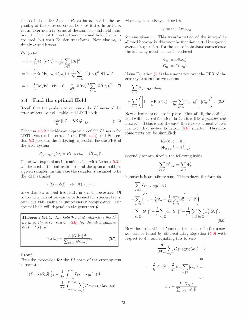
5.4 Find the optimal Hold
Recall that the goals is to minimize the L2 norm of theerror system over all stable and LDTI holds:
minH
||(I −HS)G||L2 (5.6)
Theorem 4.3.2 provides an expression of the L2 norm forLDTI systems in terms of the FPR (4.4) and Subsec-tion 5.3 provides the following expression for the FPR ofthe error system
P(I−HS)G(ω) = PI−HS(ω) · |G(iω)|2.
These two expressions in combination with Lemma 5.3.1will be used in this subsection to find the optimal hold fora given sampler. In this case the sampler is assumed to bethe ideal sampler
ψ(t) = δ(t) ⇔ Ψ(iω) = 1
since this one is used frequently in signal processing. Ofcourse, the derivation can be performed for a general sam-pler, but this makes it unnecessarily complicated. Theoptimal hold will depend on the generator G.
Theorem 5.4.1. The hold H∗ that minimizes the L2
norm of the error system (5.6) for the ideal samplerψ(t) = δ(t), is
Φ∗(iω) =h |G(iω)|2
∑
k∈Z|G(iωk)|2 . (5.7)
ProofFirst the expression for the L2 norm of the error systemis rewritten
||(I −HS)G||2L2 =1
2π
∫ ∞
−∞
P(I−HS)G(ω) dω
=1
2π
∫ ωnyq
−ωnyq
∑
n∈Z
P(I−HS)G(ωn) dω
where ωn is as always defined as
ωn := ω + 2nωnyq
for any given ω. This transformation of the integral isallowed because in this way the function is still integratedover all frequencies. For the sake of notational conveniencethe following notations are introduced
Φn := Φ(iωn)
Gn := G(iωn).
Using Equation (5.3) the summation over the FPR of theerror system can be written as
∑
n∈Z
P(I−HS)G(ωn)
=∑
n∈Z
([
1 − 2
hRe (Φn) +
1
h2
∑
k∈Z
|Φn+k|2]
|Gn|2)
. (5.8)
Now a few remarks are in place. First of all, the optimalhold will be a real function, in fact it will be a positive realfunction. If this is not the case, there exists a positive realfunction that makes Equation (5.8) smaller. Thereforesome parts can be simplified:
Re (Φn) = Φn
|Φn+k|2 = Φ2n+k.
Secondly for any fixed n the following holds
∑
k∈Z
Φ2n+k =
∑
k∈Z
Φ2k
because it is an infinite sum. This reduces the formula∑
n∈Z
P(I−HS)G(ωn)
=∑
n∈Z
([
1 − 2
hΦn +
1
h2
∑
k∈Z
Φ2k
]
|Gn|2)
=∑
n∈Z
|Gn|2 −2
h
∑
n∈Z
Φn|Gn|2 +1
h2
∑
n∈Z
∑
k∈Z
Φ2k|Gn|2.
(5.9)
Now the optimal hold function for one specific frequencyωm can be found by differentiating Equation (5.9) withrespect to Φm and equalling this to zero
∂
∂Φm
∑
n∈Z
P(I−HS)G(ωn) = 0
⇔
0 − 2
h|Gm|2 +
2
h2Φm
∑
n∈Z
|Gn|2 = 0
⇔
Φm =h |Gm|2
∑
n∈Z|Gn|2
.
23

This means that the optimal hold H∗ is
Φ∗(iω) =h |G(iω)|2
∑
k∈Z|G(iωk)|2 .
This is the same result as shown in [4] but the derivationis different.
5.5 Comparison with other Holds
The great advantage of the optimal hold (5.7) comparedto standard holds like the zero- or first-order hold, is thatit changes if the generator G changes. This will be demon-strated by a few examples. To compare the optimal hold,several frequently used holds are exploited in these exam-ples. Recall the zero-order hold
φ(t) = 1[0,h](t)
the first-order hold
φ(t) =
(
1 − |t|h
)1[−h,h](t)
and the sinc holdφ(t) = sinc(t)
from Subsection 2.1.2.
Example 5.5.1. Consider the same system G as in Ex-ample 2.5.1 on page 8:
G(s) =1
s+ 1.
The L2 system norm of (I −HS)G will be calculated fordifferent holds using Theorem 4.3.2. The sampler is as-sumed to be the ideal sampler ψ(t) = δ(t) and the sam-pling period h equals 1. The optimal hold is comparedwith the zero-order hold, the first-order hold and the sinchold.Figure 14 shows plots of P(I−HS)G(ω) for the differentholds. Table 1 shows the L2 norm of the error system forthe different holds.
Hold ||I − HS)G||2L2
Zero-order 0.3655First-order 0.1572
Sinc 0.1942Optimal 0.1549
Table 1: L2 norm of the error system for differentholds for the system G(s) = 1
s+1
In order to get an indication how much energy of the origi-nal system G is preserved by sampling and reconstruction,the following formula is exploited
||G||2L2 − ||(I −HS)G||2L2
||G||2L2
× 100% =0.5 − 0.1549
0.5× 100%
= 69.0%.
So 69.0% of the system’s energy is preserved by samplingand reconstruction if a sampling period h = 1 in combina-tion with the optimal hold is used. In Example 3.2.1 thepreserved energy with optimal HS was 80.4% and nowwith this fixed sampler 69.0% is the best one can do.Another explanation of the formula above is that if theinput signal is white noise (see Definition A.1.11) then69.0% of its power is preserved by sampling and recon-struction with the optimal hold in combination with thisfixed sampler and a sampling period h = 1.
0 2 4 6 8 10 12 14 160
0.05
0.1
0.15
0.2
0.25
Zero−orderFirst−orderSincOptimal
Figure 14: Plots of the FPR of (I −HS)G forG(s) = 1
s+1 , the ideal sampler and differentholds. In blue the zero-order hold, in red thefirst-order hold, in green the sinc hold and inpink the optimal hold
Example 5.5.2. Consider the same system G as in Ex-ample 3.3.1 on page 15:
G(s) =1
(s+ 0.2)2 + 1.
Similar to Example 5.5.1, the L2 system norm of(I −HS)G will be calculated for different holds using The-orem 4.3.2. The optimal hold is compared with the sameholds and again the sampler is assumed to be the idealsampler. In this example is the sampling period h = 4,unlike Example 5.5.1.Figure 15 shows plots of P(I−HS)G(ω) for the differentholds. Table 2 shows the L2 norm of the error system forthe different holds.In order to get an indication how much energy of the origi-nal system G is preserved by sampling and reconstruction,the following formula is exploited
||G||2L2 − ||(I −HS)G||2L2
||G||2L2
× 100% =1.2019− 0.5492
1.2019× 100%
= 54.3%.
24

Hold ||I − HS)G||2L2
Zero-order 2.2918First-order 1.0238
Sinc 1.6379Optimal 0.5492
Table 2: L2 norm of the error system for differentholds for the system G(s) = 1
(s+0.2)2+1
So 54.3% of the system’s energy is preserved by samplingand reconstruction if a sampling period h = 4 in combina-tion with the optimal hold is used. In Example 3.3.1 thepreserved energy with optimal HS was 65.0% and nowwith this fixed sampler 54.3% is the best one can do.Another explanation of the formula above is that if the in-put signal is white noise (see Definition A.1.11) then 54.3%of its power is preserved by sampling and reconstructionwith the optimal hold in combination with this fixed sam-pler and a sampling period h = 4.In this example the L2 norm of the error system for thesinc hold and the zero-order hold are larger than the L2
norm of the system itself ||G||2L2 = 1.2019. This meansthat it is better to take the zero hold φ(t) := 0, ∀t ∈ R be-cause then the L2 norm of the error system is smaller.
0 0.5 1 1.5 2 2.5 30
5
10
15
Zero−orderFirst−orderSincOptimal
|G(iw)|2
Figure 15: Plots of the FPR of (I −HS)G forG(s) = 1
(s+0.2)+1 , the ideal sampler and different
holds. In blue the zero-order hold, in red thefirst-order hold, in green the sinc hold, in pinkthe optimal hold and in black the response ofthe system itself |G(iω)|2
25

6 Concluding Remarks
In this report it has been achieved to calculate the L2
norm of the error system for the optimal combination ofsampler and hold for both monotonically decreasing andnon-monotically decreasing frequency response |G(iω)|2.Furthermore the graphical interpretation of this optimalcombination is presented.Next the Frequency Power Response is introduced in or-der to calculate the L2 norm of an LDTI system and ithas been proven that the L2 norm of an LDTI system canindeed be expressed in terms of this FPR. Using this ex-pression of the L2 norm of an LDTI system, the optimalhold is constructed for a given sampler and sampling pe-riod.And last, this optimal hold is compared to several otherholds. For different holds the L2 norm of the error systemis calculated and the graphical interpretation (using theFPR) of the error system for these holds is presented.
26

Appendices
A Definitions and Theorems
A.1 Classical system theory
Definition A.1.1. A system is an input/output system if
• the input u is not restricted by the system.
• the ouput y is completely determined by the input u.
Figure 16 is an illustration of an input/output system.
u yG
Figure 16: A system with input u, output y andmapping G
Definition A.1.2. A system G is said to be BIBO-stableif its output y is bounded as long as its input u is boundedas well:
|u(t)| < M1 ⇒ |y(t)| < M2.
Definition A.1.3. A system has a state space represen-tation if it can be written in the following form
x = Ax+Bu
y = Cx+Du(A.1)
where A, B and C are real matrices. Figure 17 shows theblock representation of the state space representation ofthe system.
ux x
yB1s C
A
D
+ +
Figure 17: The state space respresentation of sys-tem (A.1) with input u, output y, real matricesA, B, C and D and where 1
s denotes a pure in-tegrator
Definition A.1.4. Transforming system (A.1) to theLaplace domain gives a simple set of equations withoutderivatives (differentiating in the time domain reduces tomultiplying by s in the Laplace domain):
sX(s) = AX(s) +BU(s)
Y (s) = CX(s) +DU(s).
Substituting the solution of X(s) of the first equation inthe second equation (provided that the inverse of (sI−A)exists) leads to a transfer function G(s) that maps theinput u on the output y:
Y (s) = [C(sI −A)−1B +D]U(s)
Y (s) = G(s)U(s)
which often has the following notation
y = G(s)u.
Definition A.1.5. For a real transfer matrix G the con-jugate is defined as:
G∼(s) := [G(−s)]T .
Furthermore this conjugate is used to computate the mag-nitude of the frequency response of the transfer function:
|G(iω)|2 = G∼(iω)G(iω)
Definition A.1.6. A system G is said to be linear if
G(λ1y1 + λ2y2) = λ1Gy1 + λ2Gy2
for every two inputs y1, y2 and scalars λ1, λ2.
Definition A.1.7. To define continuous time invariance,first the continuous time shift of a signal στ is defined:
(στ f)(t) := f(τ + t).
A system G is said to be Linear Continuous Time Invari-ant (LCTI) if it is linear (see Definition A.1.6) and if
G(στ ) = στ (G)
holds for every τ ∈ R.
Definition A.1.8. To define discrete time invariance, thediscrete time shift of a signal σk is defined:
(σkf)(t) := f(kh+ t)
for a fixed h ∈ R.A system G is said to be Linear Discrete Time Invariant(LDTI) if it is linear (see Definition A.1.6) and if
G(σk) = σk(G)
holds for every k ∈ Z.
Definition A.1.9. A signal f : R → C is said to be causalif f(t) = 0 for all t < 0.
27

Definition A.1.10. The convolution of two contin-uous signals f : R → C and g : R → C is the signal(f ∗ g) : R → C defined as
(f ∗ g)(t) :=
∫ ∞
−∞
f(τ)g(t− τ)dτ.
Definition A.1.11. A signal w(t) is said to be white noiseif its expectation equals zero:
E(w(t)) = 0
and its standard deviation equals σ:
E(w(t)w(s)) = σ2δ(t− s).
28
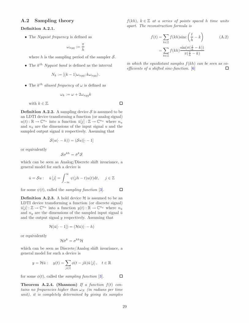
A.2 Sampling theory
Definition A.2.1.
• The Nyquist frequency is defined as
ωnyq :=π
h
where h is the sampling period of the sampler S.
• The kth Nyquist band is defined as the interval
Nk := [(k − 1)ωnyq; kωnyq) .
• The kth aliased frequency of ω is defined as
ωk := ω + 2ωnyqk
with k ∈ Z.
Definition A.2.2. A sampling device S is assumed to bean LDTI device transforming a function (or analog signal)u(t) : R → Cnu into a function u[j] : Z → Cnu where nu
and nu are the dimensions of the input signal u and thesampled output signal u respectively. Assuming that
S(u(· − h)) = (Su)[· − 1]
or equivalently
Sσkh = σkSwhich can be seen as Analog/Discrete shift invariance, ageneral model for such a device is
u = Su : u [j] =
∫ ∞
−∞
ψ(jh− t)u(t)dt, j ∈ Z
for some ψ(t), called the sampling function [3].
Definition A.2.3. A hold device H is assumed to be anLDTI device transforming a function (or discrete signal)u[j] : Z → Cnu into a function y(t) : R → Cny where nu
and ny are the dimensions of the sampled input signal uand the output signal y respectively. Assuming that
H(u[· − 1]) = (Hu)(· − h)
or equivalentlyHσk = σkhH
which can be seen as Discrete/Analog shift invariance, ageneral model for such a device is
y = Hu : y(t) =∑
j∈Z
φ(t− jh)u [j] , t ∈ R
for some φ(t), called the sampling function [3].
Theorem A.2.4. (Shannon) If a function f(t) con-tains no frequencies higher than ωN (in radians per timeunit), it is completely determined by giving its samples
f(kh), k ∈ Z at a series of points spaced h time unitsapart. The reconstruction formula is
f(t) =∑
k∈Z
f(kh)sinc
(
t
h− k
)
(A.2)
=∑
k∈Z
f(kh)sin(π( t
h − k))
π( th − k)
in which the equidistant samples f(kh) can be seen as co-efficients of a shifted sinc-function. [6]
29

A.3 General mathematics
Definition A.3.1. A real-valued function
||·|| : F → R
is called a norm on a vector space F if it satisfies
1. ||f || ≥ 0 for all f ∈ F , and ||f || = 0 ⇔ f = 0
2. ||λf || = |λ| · ||f || for all λ ∈ R and f ∈ F3. ||f + g|| ≤ ||f || + ||g|| for all f, g ∈ F .
If all these assumptions hold for all elements of F , then Fis called a vector space.
Definition A.3.2. A complex-valued function
〈·, ·〉 : F × F → C
is called a (complex) inner product on a vector space F ifit satisfies
• 〈f + g, h〉 = 〈f, h〉 + 〈g, h〉 for all f, g, h ∈ F• 〈λf, g〉 = λ 〈f, g〉 for all λ ∈ R and f, g ∈ F• 〈f, g〉 = 〈g, f〉 for all f, g ∈ F• 〈f, f〉 > 0 if f 6= 0, while 〈f, f〉 = 0 for f = 0.
If all these assumptions hold for all elements of F , then Fis called an inner product space.
Note that every inner product space is an normed spaceas well; by taking the norm of an element as the squareroot of the inner product of the element with itself:
||·|| =√
〈·, ·〉.Definition A.3.3. The L2-space is a vector space consist-ing of all functions f : [a, b] → R for certain a and b ∈ R.A function f : [a, b] → R is an element of L2[a, b] if
∫ b
a
|f(t)|2 dt <∞.
If additionally a and b equal −∞ and ∞ respectively thenthe space is denoted as L2(R).The standard L2-norm of f ∈ L2[a, b] is the mapping||·||L2 : L2[a, b] → R defined as
||f ||L2 :=
√
∫ b
a
|f(t)|2 dt.
Definition A.3.4. Another frequently used norm in sig-nal theory is the L∞-norm.A function f : R → R is an element of L∞(R) if
ess supt∈R
|f(t)| <∞.
The standard L∞-norm of f ∈ L∞(R) is defined as
||f ||L∞ := ess supt∈R
|f(t)|.
Definition A.3.5. Let f(t) be an absolutely integrablefunction. Then the following Fourier integral:
F (iω) =
∫ ∞
−∞
f(t)e−iωtdt
exists for all ω ∈ R and its inverse is given by
f(t) =1
2π
∫ ∞
−∞
F (iω)eiωtdω.
The Fourier transform of f(t) is always denoted by a cap-ital: F (iω).
Theorem A.3.6. (Parseval) Let f(t) be a square inte-grable function, then
∫ ∞
−∞
|f(t)|2 dt =1
2π
∫ ∞
−∞
|F (iω)|2 dω. (A.3)
Definition A.3.7. The principal logarithm of a squarematrix A without eigenvalues on the branch cut (the neg-ative real axis, including zero) is defined as the unique ma-trix B := log(A) for which eB = A and whose spectrumlies in the open horizontal strip z ∈ C|−π < Im (z) < πof the complex plane [2, 5].
Definition A.3.8. A matrix A is called stable if it issquare and all its eigenvalues lie in the left open half ofthe complex plane C:
Re (λi) < 0 ∀i.
30

A.4 Lifting theory
Definition A.4.1. For any signal f : R → Cnf , the lifting
f : Z → [0, h) → Cnf is the sequence of functions f [k]defined as [3]
f [k](τ) = f(kh+ τ), k ∈ Z, τ ∈ [0, h).
Definition A.4.2. The (lifted) Fourier transform Ffof a lifted function f is defined as
Ff = f(eiωh; τ) :=∑
k∈Z
f [k] (τ)e−iωkh
where the frequency ω is 2π-periodic [3].
Theorem A.4.3. (Key lifting formula) Let f ∈ L2(R).Then the lifted Fourier transform can be determined fromthe classic Fourier transform via:
f(eiωh; τ) =1
h
∑
k∈Z
F (iωk)eiωkτ
for all τ ∈ [0, h), where ωk = ω + 2ωNk. And its inverseis given by [3]
F (iωk) =
∫ h
0
f(eiωh; τ)e−iωkτdτ.
31

References
[1] R.E. Bellman and R.S. Roth. The Laplace Transform.World Scientific, 1984.
[2] N. J. Higham. Functions of Matrices: Theory andComputation. Society for Industrial and AppliedMathematics, 2008.
[3] G. Meinsma and L. Mirkin. Sampling from a system-theoretical viewpoint: part 1 - concepts and tools.IEEE Trans. on Signal Processing, 58, issue 7:3578–3590, July 2010.
[4] G. Meinsma and L. Mirkin. Sampling from a system-theoretical viewpoint: part 2 - noncausal solutions.IEEE Trans. on Signal Processing, 58, issue 7:3591–3606, July 2010.
[5] G. Meinsma and H. S. Shekawat. Frequency-truncatedsystem norms. Automatica, 47, issue 8:1842–1845, May2011.
[6] M. Unser. Sampling - 50 years after shannon. Proceed-ings of the IEEE, 88, issue 4:569–587, April 2000.
32