Embed Size (px)
Citation preview
Optimal Portfolio Selection using Regularization�
Marine Carrasco and Nérée NoumonUniversité de Montréal
June 2012Preliminary and incomplete
Abstract
The mean-variance principle of Markowitz (1952) for portfolio selection givesdisappointing results once the mean and variance are replaced by their samplecounterparts. The problem is ampli�ed when the number of assets is large andthe sample covariance is singular or nearly singular. In this paper, we investigatefour regularization techniques to stabilize the inverse of the covariance matrix: theridge, spectral cut-o¤, Landweber-Fridman and LARS Lasso. These four methodsinvolve a tuning parameter that needs to be selected. The main contribution is toderive a data-driven method for selecting the tuning parameter in an optimal way,i.e. in order to minimize the expected loss in utility of a mean-variance investor.The cross-validation type criterion takes a similar form for the four regularizationmethods. The resulting regularized rules are compared to the sample-based mean-variance portfolio and the naive 1/N strategy in terms of in-sample and out-of-sample Sharpe ratio and expected loss in utility. The main �nding is that aregularization to covariance matrix drastically improves the performance of mean-variance problem and outperforms the naive portfolio especially in ill-posed cases,as demonstrated through extensive simulations and empirical study.
Keywords: Portfolio selection, mean-variance analysis, estimation error, regularization,model selection.JEL subject Classi�cation: G11, C52, C58
�We thank Raymond Kan, Bruce Hansen, and Marc Henry for their helpful comments.
1 Introduction
In his seminal paper of 1952, Markowitz stated that the optimal portfolio selectionstrategy should be an optimal trade-o¤ between return and risk instead of an expectedreturn maximization only. In his theoretical framework, Markowitz made the importantassumption that the beliefs about the future performance of asset returns are known.However in practice these beliefs have to be estimated. The damage caused by the so-called parameter uncertainty has been pointed out by many authors, see for instance Kanand Zhou (2007). Solving the mean-variance problem leads to estimate the covariancematrix of returns and take its inverse. This results in estimation error, ampli�ed by twofacts. First, the number of securities is typically very high and second, these securityreturns may be highly correlated. This results in an ill-posed problem in the sensethat a slight change in portfolio return target implies a huge change in the optimalportfolio weights. In-sample, these instabilities are expressed by the fact that the sampleminimum-variance frontier is a highly biased estimator of the population frontier asshown by Kan and Smith (2008); out-of-sample, the resulting rules are characterized byvery poor performances. To tackle these issues, various solutions have been proposed.Some authors have taken a Bayesian approach, see Frost and Savarino (1986). Some haveused shrinkage, more precisely Ledoit and Wolf (2003, 2004a,b) propose to replace thecovariance matrix by a weighted average of the sample covariance and some structuredmatrix. Tu and Zhou (2009) take a combination of the naive 1/N portfolio with theMarkowitz portfolio. Alternatively, Brodie, Daubechies, De Mol, Giannone and Loris(2008) and Fan, Zhang, and Yu (2009) use a method called Lasso which consists inimposing a constraint on the sum of the absolute values (l1 norm) of the portfolioweights. The l1�constraint generalizes the shortsale constraint of Jagannathan and Ma(2003) and generates sparse portfolios which degree of sparsity depends on a tuningparameter. Recently, a general and uni�ed framework has been proposed by DeMiguel,Garlappi, Nogales and Uppal (2009) in terms of norm-constrained minimum-varianceportfolio that nests all the rules cited above. A new promising approach introduced byBrandt, Santa-Clara and Valkanov (2009) avoid the di¢ culties in the estimation of assetreturns moments by modelling directly the portfolio weight in each asset as a functionof the asset�s characteristics.In this paper, we investigate various regularization (or stabilization) techniques bor-
rowed from the literature on inverse problems. Indeed, inverting a covariance matrix canbe regarded as solving an inverse problem. Inverse problems are encountered in many�elds and have been extensively studied, see Carrasco, Florens, and Renault (2007) fora review. Here, we will apply the three regularization techniques that are the mostused: the ridge which consists in adding a diagonal matrix to the covariance matrix, thespectral cut-o¤ which consists in discarding the eigenvectors associated with the small-est eigenvalues, and Landweber Fridman iterative method. For completeness, we alsoconsider a form of Lasso where we penalize the l1 norm of the optimal portfolio weights.
1
These various regularization techniques have been used and compared in the context offorecasting macroeconomic time series using a large number of predictors by i.e. Stockand Watson (2002), Bai and Ng (2008), and De Mol, Giannone, and Reichlin (2008).The four methods under consideration involve a regularization (or tuning) parameterwhich needs to be selected. Little has been said so far on how to choose the tuning pa-rameter to perform optimal portfolio selection. For example using the Lasso, Brodie etal. (2008), Fan et al. (2009) show that by tuning the penalty term one could constructportfolio with desirable sparsity but do not give a systematic rule on how to select it inpractice. Ledoit and Wolf (2004) choose the tuning parameter in order to minimize themean-square error of the shrinkage covariance matrix, however this approach may notbe optimal for portfolio selection. DeMiguel et al (2009) calibrate the upper bound onthe norm of the minimum variance portfolio weights, by minimizing portfolio varianceor by maximizing the last period out-of-sample portfolio return. Their calibrations maybe improved by considering an optimal trade-o¤ between portfolio risk and return.The main objective of this paper is to derive a data-driven method for selecting
the regularization parameter in an optimal way. Following the framework of Kan andZhou (2008), we suppose that the investor is characterized by a mean-variance utilityfunction and would like to minimize the expected loss incurred in using a particularportfolio strategy. The mean-variance investor approach nests di¤erent problems suchas the minimum-variance portfolio considered in DeMiguel et al (2009) and Fan et al.(2009), the mean-variance portfolio considered in Brodie et al (2009) and the tangencyportfolio. The expected loss can not be derived analytically. Our contribution is toprovide an estimate of the expected loss in utility that uses only the observations. Thisestimate is a bias-corrected version of the generalized cross-validation criterion. Theadvantage of our criterion is that it applies to all the methods mentioned above andgives a basis to compare the di¤erent methods.The rest of the paper is organized as follows. Section 2 reviews the mean-variance
principle. Section 3 describes three regularization techniques of the inverse of the covari-ance matrix. Section 4 discusses stabilization techniques that take the form of penalizedleast-squares. Section 5 derives the optimal selection of the tuning parameter. Section6 presents simulations results and Section 7 empirical results. Section 8 concludes.
2 Markowitz paradigm
Markowitz (1952) proposes the mean-variance rule, which can be viewed as a trade-o¤between expected return and the variance of the returns. For a survey, see Brandt(2009). Consider N risky assets with random return vector Rt+1 and a riskfree assetwith known return Rft . De�ne the excess returns rt+1 = Rt+1�Rft :We assume that theexcess returns are independent identically distributed with mean and covariance matrixdenoted by � and �, respectively. The investor allocates a fraction x of wealth to risky
2

assets and the remainder (1� 10Nx) to the risk-free asset, where 1N denotes a N�vectorof ones. The portfolio excess return is therefore x0rt+1: The investor is assumed to choosethe vector x to maximize the mean-variance utility function
U (x) = x0��
2x0�x (1)
where is the relative risk aversion. The optimal portfolio is given by
x� =1
��1�: (2)
In order to solve the mean variance problem (1), the expected return and the covari-ance matrix of the vector of security return, which are unknown, need to be estimatedfrom available data set. In particular, an estimate of the inverse of the covariance matrixis needed. The sample covariance may not be appropriate because it may be nearly sin-gular, and sometimes not even invertible. The issue of ill-conditioned covariance matrixmust be addressed because inverting such matrix increases dramatically the estimationerror and then makes the mean variance solution unreliable. Many regularization tech-niques can stabilize the inverse. They can be divided into two classes: regularizationdirectly applied to the covariance matrix and regularization expressed as a penalizedleast-squares.
3 Regularization as approximation to an inverse prob-lem
3.1 Inverse problem
Let rt, t = 1; � � � ; T be the observations of asset returns and R be the T � N matrixwith tth row given by r0t. Let = E (rtr
0t) = E (R0R) =T:
��1� = (� ��0)�1�
=
��1 +
�1��0�1
1� �0�1�
��
=�1�
1� �0�1�
where the second equality follows from the updating formula for an inverse matrix (seeGreene, 1993, p.25). Hence
x� =�1�
(1� �0�1�)=
�
(1� �0�)(3)
3

where� = �1� = E (R0R)
�1E (R01T ) : (4)
We can replace the unknown expectation � by the sample average � = 1T
PTt=1 rt and the
covariance � by the sample covariance � = (R� 1T �0)0 (R� 1T �0) =T � ~R0 ~R: Replacing� and � by their sample counterparts, one obtains the sample based optimal allocationbx = ��1�= : Jobson and Korkie (1983, Equation (15)) and later Britten-Jones (1999)showed that bx can be rewritten as
bx = �=� �1� �0�
��where � is the OLS estimate of � in the regression
1 = �0rt+1 + ut+1
or equivalently1T = R� + u (5)
where R is the T �N matrix with rows composed of r0t. In other words, one should notcenter rt in the calculation of x�. Finding � can be thought of as �nding the minimumleast-squares solution to the equation:
R� = 1T : (6)
It is a typical inverse problem.The stability of the previous problem depends on the characteristics of the matrix
= R0R=T . Two di¢ culties may occur: the assets could be highly correlated (i.e. thepopulation covariance matrix � is nearly singular) or the number of assets could be toolarge relative to the sample size (i.e. the sample covariance is (nearly) singular eventhough the population covariance is not). In such cases, typically has some singularvalues close to zero resulting in an ill posed problem, such that the optimization ofthe portfolio becomes a challenge. These di¢ culties are summarized by the conditionnumber which is the ratio of the maximal and minimal eigenvalue of . A large conditionnumber leads to unreliable estimate of the vector of portfolio weights x.The inverse problem literature, that usually deals with in�nite dimensional problems,
has proposed various regularization techniques to stabilize the solution to (6). For anoverview on inverse problems, we refer the readers to Kress (1999) and Carrasco, Flo-rens, and Renault (2007). We will consider here the three most popular regularizationtechniques: ridge, spectral cut-o¤, and Landweber Fridman. Each method will give a dif-ferent estimate of �, denoted �� and estimate of x
�, denoted bx� = ��=� �1� �0��
��:
The T � N matrix R can be regarded as an operator from RN (endowed with theinner product hv; wi = v0w) into RT (endowed with the inner product h�; 'i = �0'=T ).
4

The adjoint of R is R0=T: Let��j; �j; vj
�; j = 1; 2; :::; N be the singular system of R,
i.e. R�j = �j vj, R0vj=T = �j�j, moreover��2
j ; �j
�are the eigenvalues and orthonor-
mal eigenvectors of R0R=T and��2
j ; vj
�are the nonzero eigenvalues and orthonormal
eigenvectors of RR0=T: If N < T , it is easier to compute �j and �2
j , j = 1; :::; N theorthonormal eigenvectors and eigenvalues of the matrix R0R=T and deduce the spectrumof RR0=T: Indeed, the eigenvectors of RR0 are vj = Rb�j=�j associated with the samenonzero eigenvalues �
2
j . Let � > 0 be a regularization parameter.
3.2 Ridge regularization
The Ridge regression has been introduced by Hoerl and Kennard (1970) as a more stablealternative to the standard least-squares estimator with potential lower risk. It consistsin adding a diagonal matrix to R0R=T .
�� =
�R0R
T+ �I
��1R01TT
; (7)
�� =NXj=1
�j
�2
j + �(10Tbvj) �j:
This regularization has a Bayesian interpretation, see i.e. De Mol et al (2008).
3.3 Spectral cut-o¤ regularization
This method discards the eigenvectors associated with the smallest eigenvalues.
�� =Xb�2j>�
1b�j (10Tbvj) b�j:Interestingly, bvj are the principal components of , so that if rt follows a factor model,bv1, bv2,... estimate the factors.3.4 Landweber-Fridman regularization
Let c be a constant such that 0 < c < 1= kRk2 where kRk is the largest eigenvalue of R:The solution to (6) can be computed iteratively as
k =
�I � c
R0R
T
� k�1 + c
R01TT
; k = 1; 2; :::; 1=� � 1
5

with 0 = cR01T=T . Alternatively, we can write
�� =X 1b�j
�1�
�1� cb�2j�1=�� (10Tbvj) b�j:
Here, the regularization parameter � is such that 1=� � 1 represents the number ofiterations.The three methods involve a regularization parameter � which needs to converge to
zero with T at a certain rate for the solution to converge.
3.5 Explicit expression of estimators
For the three regularizations considered above, we have
Rb�� =MT (�) 1T
with
MT (�)w =TXj=1
q�� ; �
2
j
�(w0bvj) bvj
for any T� vectors w. Moreover, trMT (�) =PT
j=1 q�� ; �
2
j
�. The function q takes
a di¤erent form depending on the type of regularization. For Ridge, q�� ; �
2
j
�=
�2
j=��2
j + ��: For Spectral cut-o¤, q
�� ; �
2
j
�= I
��2
j � ��. For Landweber Fridman,
q�� ; �
2
j
�= 1�
�1� c�
2
j
�1=�.
3.6 Related estimator: Shrinkage
In this subsection, we compare our methods with a popular alternative called shrinkage.Shrinkage can also be regarded as a form of regularization. Ledoit and Wolf (2003)propose to estimate the returns covariance matrix by a weighted average of the samplecovariance matrix � and an estimator with a lot of structure F; based on a model.The �rst one is easy to compute and has the advantage to be unbiased. The secondone contains relatively little estimation error but tends to be misspeci�ed and can beseverely biased. The shrinkage estimator takes the form of a convex linear combination :�F+(1��)�, where � is a number between 0 and 1. This method is called shrinkage sincethe sample covariance matrix is shrunk toward the structured estimator. � is referred toas the shrinkage constant. With the appropriate shrinkage constant, we can obtain anestimator that performs better than either extreme (invertible and well-conditioned).Many potential covariance matrices F could be used. Ledoit and Wolf (2003) sug-
gested the single factor model of Sharpe (1963) which is based on the assumption that
6
stock returns follow the model (Market model):
rit = �i + �ir0t + "it
where residuals �it are uncorrelated to market returns r0t and to one another, with aconstant variance V ar(�it) = �ii. The resulting covariance matrix is
� = �20��0 +�
Where �20 is the variance of market returns and � = diag(�ii). �20 is consistentlyestimated by the sample variance of market returns, � by OLS, and �ii by the residualvariance estimate. A consistent estimate of � is then
F = s20bb0 +D:
Instead of using the F derived from a factor model, one can use the constant correlationmodel1 (Ledoit and Wolf (2004a)) or the identity matrix F = I (Ledoit and Wolf(2004b)). They give comparable results but are easier to compute.In the particular case where the shrinkage target is the identity matrix, the shrinkagemethod is equivalent to Ridge regularization since the convex linear combination �I +(1� �)� can be rewritten :
�Shrink = c��+�I
�;
and��1Shrink =
��+�I
��1=c;
where c is a constant.Once the shrinkage target is determined one has to choose the Optimal Shrinkage
intensity ��. Ledoit and Wolf (2004b) propose to select �� so that it minimizes theexpected L2 distance between the resulting shrinkage estimator �Shrink = �
�F+(1���)�
and the true covariance matrix �. The limitation of this criterion is that it only focuseson the statistical properties of �, and in general could fail to be optimal for the portfolioselection.
4 Regularization scheme as penalized least-square
The traditional optimal Markowitz portfolio x� is obtained from (3) and
� = argmin�Ehj1� �0rtj2
i1All the pairwise covariances are identical.
7

If one replaces the expectation by the sample average �; the problem becomes:
� = argmin�k1T �R�k22 (8)
As mentioned before, the solution of this problem may be very unreliable if R0R isnearly singular. To avoid having explosive solutions, we can penalize the large values byintroducing a penalty term applied to a norm of �. Depending on the norm we choose,we end up with di¤erent regularization techniques.
4.1 Bridge method
For & > 0 the Bridge estimate is given by
b�� = argmin�k1T�R�k22 + �
NXi=1
j�ij&
where � is the penalty term.The Bridge method includes two special cases. For & = 1 we have the Lasso regu-
larization, while & = 2 leads to the Ridge method. The termNPi=1
jxij& can be interpretedas a transaction cost. It is linear for Lasso, but quadratic for the ridge. The portfoliowill be sparse as soon as & � 1. The objective function is strictly convex when & > 1,convex for & = 1 and no longer convex for & < 1: The case with & < 1 is considered inHuang, Horowitz, and Ma (2008), but will not be examined any further here.
4.2 Least Absolute Shrinkage and Selection Operator (LASSO)
The Lasso regularization technique introduced by Tibshirani (1996) is the l1-penalizedversion of the problem (8). The Lasso regularized solution is obtained by solving:
b�� = argmin�k1T �R�k22 + � k�k1 :
The main feature of this regularization scheme is that it induces sparsity. It hasbeen studied by Brodie, Daubechies, De Mol, Giannone and Loris (2008) to computeportfolio involving only a small number of securities. For two di¤erent penalty constants� 1 and � 2 the optimal regularized portfolio satis�es: (� 1� � 2)
� �[�2] 1� �[�1]
1
�� 0
then the higher the l1-penalty constant (�), the sparser the optimal weights. So that aportfolio with non negative entries corresponds to the largest values of � and thus tothe sparsest solution. In particular the same solution can be obtained for all � greaterthan some value � 0.
8

Brodie et al. consider models without a riskfree asset. Using the fact that all thewealth is invested (x01N = 1), they use the equivalent formulation for the objectivefunction as:
k1T �Rxk22 + 2�X
i with xi<0
jxij+ �
which is equivalent to a penalty on the short positions. The Lasso regression thenregulates the amount of shorting in the portfolio designed by the optimization process,so that the problem stabilizes. For a value of � su¢ ciently large, all the components ofx will be nonnegative, thus excluding short-selling. This gives a rationale for the �ndingof Jagannathan and Ma (2003). Jagannathan and Ma found that imposing the no short-selling constraint improves the performance of portfolio selection. This constraint actsas a regularization on the portfolio weights.The general form of the l1-penalized regression with linear constraints is:b�� = argmin
�2Hkb� A�k22 + � k�k1
H is an a¢ ne subspace de�ned by linear constraints. The regularized optimal portfoliocan be found using an adaptation of the homotopy / LARS algorithm as described inBrodie et al (2008). In appendix A, we provide a detailed description of this algorithm.
4.3 Ridge method
Interestingly, the ridge estimator described in (7) can be written alternatively as apenalized least-squares with l2 norm. The Ridge regression is then given by
b�� = argmin�k1T �R�k22 + � k�k22 (9)
Contrary to the Lasso regularization, the Ridge does not deliver a sparse portfolio,but selects all the securities with possibly short-selling.
5 Optimal selection of the regularization parameter
5.1 Loss function of estimated allocation
It is natural to think that the investor would like to select the parameter � that maxi-mizes the expected utility E (U (x� )) or equivalently minimizes the expected Loss func-
9
tion E (LT (�)) where
LT (�) = U (x�)� U (x� )
= (x� � x� )0 �+
2(x0��x� � x�0�x�)
= (x� � x� )0 (�� �x�) +
2(x� � x�)0� (x� � x�)
=
2(x� � x�)0� (x� � x�) : (10)
Our goal is to give a convenient expression for the criterion E (LT (�)). Consider bx� =��=
� �1� �0��
��where �� is given byb�� = b�1� R01T=T (11)
where b�1� is a regularized inverse of = R0R=T . Using the notation (3); the optimalallocation x� can be written as �= ( (1� �0�)) :The criterion (10) involves
(x� � x�) =��
1� �0��� �
1� �0�
=�� � ��
1� �0��
�(1� �0�)
��� (�
0�)� ���0��
��1� �0��
�(1� �0�)
: (12)
Note that j�0�j < 1 by construction. To evaluate (10), we need to evaluate the rateof convergence of the di¤erent terms in its expansion. To do so, we assume that � (orequivalently �) satis�es some regularity condition. This condition given in Assumption Ais similar in spirit to the smoothness condition of a function in nonparametric regressionestimation for instance. However contrary to a smoothness condition that would concernonly �, this condition relates the properties of � to those of . It implies that � belongsto the range of �=2: This type of conditions can be found in Carrasco, Florens, andRenault (2007) and Blundell, Chen, and Kristensen (2007) among others.Assumption A. (i) For some � > 0, we have
NXj=1
�; �j
�2�2�+4j
<1
where �j and �2j denote the eigenvectors and eigenvalues of .
(ii) � is Hilbert Schmidt (its eigenvalues are square summable).
Assumption A(i) is equivalent toPN
j=1
h�;�ji2�2�j
<1 because � = �1�.
Assumption A implies in particular that k�k2 <1. Let �� be de�ned as E��� jR
�where E (:jR) is the orthogonal projection on R.
10

Proposition 1 Under Assumption A and assuming N and T go to in�nity, we have
2 (1� �0�)2E�(x� � x�)0� (x� � x�)
�� 1
TE R��� � �
� 2 + (�0 (�� � �))2
(1� �0�):
The proof of Proposition 1 is given in Appendix B.
5.2 Cross-validation
From Proposition 1, it follows that minimizing E (LT (�)) is equivalent to minimizing
1
TE R��� � �
� 2 (13)
+(�0 (�� � �))2
(1� �0�): (14)
Terms (13) and (14) depend on the unknown � and hence need to be approximated.Interestingly, (13) is equal to the prediction error of model (5) plus a constant and hasbeen extensively studied. To approximate (13), we use results on cross-validation fromCraven and Wahba (1979), Li (1986, 1987), and Andrews (1991) among others.The rescaled MSE
1
TE
� R�b�� � �� 2�
can be approximated by generalized cross validation criterion:
GCV (�) =1
T
k(IT �MT (�)) 1Tk2
(1� tr (MT (�)) =T )2 :
Using the fact that
�0 (�� � �) =10TT(MT (�)� IT )R�;
(14) can be estimated by plug-in:�10T (MT (�)� IT )R�e�
�2T 2�1� �0�e�
� (15)
where �e� is an estimator of � obtained for some consistent ~� (~� can be obtained byminimizing GCV (�)). Note that the expression of (15) does not presume anything onthe regularity of � (value of �).
11
The optimal value of � is de�ned as
� = arg min�2HT
8><>:GCV (�) +�10T (MT (�)� IT )R�e�
�2T 2�1� �0�e�
�9>=>;
where HT = f1; 2; :::; Tg for spectral cut-o¤ and Landweber Fridman and HT = (0; 1)for Ridge.The Lasso estimator does not take the simple form (11). However, Tibshirani (1996)
shows that it can be approximated by a ridge type estimator and suggests using thisapproximation for cross-validation. Let ~� (�) be the Lasso estimator for a value � . Bywriting the penalty
P���j�� as P �2j=���j��, we see that ~� (�) can be approximated by
�� =�R0R + � (c)W� (�)
��1R01T
where c is the upper boundP���j�� in the constrained problem equivalent to the penal-
ized Lasso and W (�) is the diagonal matrix with diagonal elements���~�j (�)��� ; W� is the
generalized inverse of W and � (c) is chosen so thatP
j
����j �� = c: Since � (c) representsthe Lagrangian multiplier on the constraint
Pj
����j �� � c, we always have this constraintbinding when � (c) 6= 0 (ill-posed cases). Let
p (�) = trnR�R0R + � (c)W� (�)
��1R0o:
The generalized cross-validation criterion for Lasso is
GCV (�) =1
T
1T �Re� (�) 2(1� p (�) =T )2
:
Tibshirani (1996) shows in simulations that the above formula gives good results.
5.3 Optimality
Let L�T (�) =1T
R��� � �� 2 + (�0(����))
2
1��0� ; hence LT (�) = L�T (�) + rest (�) (where
rest (�) is de�ned as LT (�)� L�T (�)): Let R�T (�) = EL�T (�) :
Assumption B. (i) ut in the regression 1 = �0rt + ut is independent, identicallydistributed with mean (1� �0�) and E (u2t ) = !2. Moreover, E (utrt) = 0:(ii) Eu4mt <1;(iii)
P�2HT (TR
�T (�))
�m ! 0 for some natural number m,(iv) N diverges to in�nity as T goes to in�nity and NT�1=(�+2) goes to zero.
12

Note that the model in Assumption B(i) should not be regarded as an economicmodel. It is an arti�cial regression for which the assumptions on ut are consistent withour assumptions on rt and the fact that � = E (R0R)�1E (R01) :Using the same argument as in Li (1987, (2.5)), it can be shown that a su¢ cient
condition for B(iii) for spectral cut-o¤ and m = 2 is
inf�2HT
TR�T (�)!1:
This condition is satis�ed under Assumption A (see Lemma 3 in Appendix).
Proposition 2 Under Assumptions A and B, our selection procedure for � in the caseof Spectral Cuto¤ is asymptotically optimal in the sense that
LT (�)
inf�2HT LT (�)! 1 in probability.
The proof of Proposition 2 draws from that Li (1987) for discrete sets HT . However,it requires some adjustments for two reasons. First, our residual ut does not have meanzero. On the other hand, E (utrt) = 0 and we will exploit this equality in our proof.Second, it is usual to prove optimality by assuming that the regressors are deterministicor alternatively by conditioning on the regressors. Here, we can not condition on theregressors because, given rt, ut is not random. Hence, we have to proceed uncondition-ally. So far, we have established the asymptotic optimality of SC only. The same proofcould be used for LF with possibly additional assumptions. We are planning to provealso the asymptotic optimality of ridge using Li (1986).
6 Simulations
In this section, we use simulated data to assess the performance of each of the investmentstrategies x�(� �). The naive 1/N portfolio is taken as a benchmark to which we comparethe regularized rules. The comparisons are made in terms of in-sample performance asin Fan and Yu (2009). For a wide range of number of observations and level of aversionto risk, we examine the in-sample expected loss in utility and the sharpe ratio. The out-of-sample performances in terms of Sharpe ratio are instead provided in the empiricalstudy.
6.1 A three-factor model
We use a three-factor model to assess the in-sample performance of our strategiesthrough a Monte Carlo study. Precisely, we suppose that the N excess returns of assetsare generated by the model:
rit = bi1f1t + bi2f2t + bi3f3t + "it for i = 1; � � � ; N (16)
13

or in a contracted form:R = BF + "
where bij are the factors loading of the ith asset on the factor fj, "i is the idiosyncraticnoise independent of the three factors and independent of each other.We assume further a trivariate normal distribution for the factor loading coe¢ cients
and for the factors: bi � N (�b;�b) and ft � N��f ;�f
�. The "i are supposed to be
normally distributed with level �i drawn from a uniform distribution, so their covariancematrix is �" = diag(�21; � � � ; �2p). As a consequence the covariance matrix of returns isgiven by:
� = B�fB0 + �"
The parameters �f ,�f , �b and �b used in the model (16) are calibrated to market datafrom July 1980 to June 2008. The data sets used consist of 20 years monthly returnsof Fama-French three factors and of 30 industry portfolio from French data library. Aspointed out in Fan et al (2008) a natural idea for estimating � is to use the least-squaresestimators of B, �f and �� and obtain a substitution estimator:
� = B�f B0 + �"
where B = RF 0(FF 0)�1 is the matrix of estimated regression coe¢ cients, �f is thecovariance matrix of the three Fama-French factors. These three factors are the excessreturn of the proxy of the market portfolio over the one-month treasury bill, the di¤er-ence of return between large and small capitalization, that capture the size e¤ect, andthe di¤erence of returns between high and low book-to-market ratios, that capture thevaluation e¤ect. We choose idiosyncratic noise to be normally distributed with standarddeviation �i uniformly distributed between 0:01 and 0:03. The calibrated values aresuch that the generated asset returns exhibit three principal components. This meansin practice that the covariance matrix of the generated returns have three dominanteigenvalues. Once generated, the factors and the factor loadings are kept �xed through-out replications. Table 1 summarizes the calibrated mean and covariance matrix for thefactors and the factors loadings.
Parameters for factor loadings Parameters for factor returns�b �b �f �f
0.9919 0.0344 0.0309 0.0005 0.0060 0.0019 0.0003 -0.00050.0965 0.0309 0.0769 0.0042 0.0014 0.0003 0.0009 -0.00030.1749 0.0005 0.0042 0.0516 0.0021 -0.0005 -0.0003 0.0012
Table 1: Calibrated parameters used in simulations
14
6.2 Estimation methods and tuning parameters
We start by a series of simulations to assess the performance of the di¤erent strategiesproposed. This is done relative to the benchmark naive 1 over N strategy and thesample based Markowitz portfolio that is well known to perform poorly. The portfoliosconsidered are the naive equally weighted portfolio (1oN), the sample-based meanvariance portfolio (M), the Lasso portfolio (L), the ridge-regularized portfolio (Rdg),the spectral cut-o¤ regularized portfolio (SC) and the Landweber-Fridman portfolio(LF) as summarized in Table 2.
# Model Abbreviations1 Naive evenly weighted portfolio 1oN2 Sample-based mean variance portfolio M3 Lasso Portfolio L4 Optimal Ridge portfolio Rdg5 Optimal Spectral cut-o¤ Portfolio SC6 Optimal Landweber-Fridman Portfolio LF
Table 2: List of investment rules
The three regularization techniques introduced to improve the optimality of thesample-based Markowitz portfolio involve a regularization parameter � and they cor-respond to the sample-based Markowitz portfolio for � = 0. So our approach can beconsidered as a generalization that aims to stabilize while improving the performance ofthe sample-based mean-variance portfolio. Here we give some insights about the e¤ectfrom tuning di¤erent regularization parameters.The ridge, the spectral cut-o¤ and the Landweber-Fridman schemes have a common
feature that they transform the eigenvalues of the returns covariance matrix so thatthe resulting estimate has a more stable inverse. This transformation is done with adamping function q(� ; �) speci�c to each approach as introduced previously.The Ridge is the easiest regularization to implement and recovers the sample-based
mean-variance minimizer for � = 0.For SC, minimizing GCV with respect to � is equivalent to minimizing with respect
to p, the number of eigenvalues ranked in decreasing order. The higher the number ofeigenvectors kept, the closer we are to the sample based Markowitz portfolio. For valuesof � lower than the smallest eigenvalue, the SC portfolio is identical to the classicalsample-based portfolio.The Landweber-Fridman regularization technique can be implemented in two equiv-
alent ways. Either we perform a certain number l of iterations or we transform theeigenvalues using the function q(1
l; �). Consequently, a larger number of iterations cor-
responds to smaller value the penalty term � that belongs to the interval ]0; 1[. Besides,
15

for a large number of iterations (� � 0) the regularized portfolio x� obtained becomesvery close to the sample-based optimal portfolio x. In the Landweber-Fridman casewe seek the optimal number of iterations so that x� is the closest to the theoreticallyoptimal rule x�. In the ill-posed case we typically have a very few number of iterationswhich corresponds to a value of � close to one. That is, x� is far from the Markowitzallocation x known to perform very poorly.In the context of lasso regularization, the e¤ect of tuning the penalty � in the l1-
penalized regression have been extensively studied Brodie et al (2009). Our approachis di¤erent in the fact that we are interested in the rule that maximizes the utility ofmean-variance investor. An additional distinction is that our rules are function of theparameter �
�derived using the unconstrained version of the Homotopy/Lars Algorithm
(see Appendix for a detailed description). For a given value of the penalty term, thealgorithm determine the number of assets (from 1 toN) to be included in the portfolio aswell as the weights associated up to a normalization. For illustration, Figure 1 plots theportfolio weights constructed using the 10 industry portfolios from Fama and Frenchdata library, against the penalty term. The data set used is the French 10 industryPortfolios from January 1990 to September 2009. We seek to determine the portfolioweights associated with each of the 10 industry portfolios. The case � = 0 corresponds tothe sample-based tangency portfolio. The higher the penalty the smaller the number ofindustries included in the optimal portfolio. Furthermore, there exists a threshold (here� � 3:3) beyond which all the industry portfolios are ruled out. By order of entrance inthe optimal portfolio, the industry considered are: HiTec, Enrgy, Hlth, NoDur, Other,Durbl, Shops, Telcm and Utils.The e¤ect of tuning � can also be captured by the shape of the bias corrected version
of the GCV criterion, GCVb; plotted in Figure 2 for a single sample with N = 100 andT = 120. In our computations, the GCVb for the Rdg the SC and the LF portfoliosare minimized respectively with respect to � , the number p of eigenvectors kept in thespectral decomposition of returns covariance matrix, and the number of iterations l.For all the regularization schemes, the function GCVb have a convex shape which is aparticularly interesting feature since it guarantees the unicity of the optimal parameter� : Another interesting pattern of the GCVb is that its curve gets steeper and giveshigher values for the parameters corresponding to the sample-based investment rule:ridge penalty term close to 0, large number of eigenvectors kept for SC or large numberof iterations for LF. This suggests that the performance of the regularized rules arealways improved relative to the sample-based rule.
6.3 In-sample performance
We perform 1000 replications. In each of the replications, model (16) is used alongwith the parameters in Table 1 to generate T = 120 monthly observations of asset ex-cess returns. We consider four di¤erent values for the number of assets traded, namely
16

Figure 1: Evolution of the tangency portfolio weights with the penalty term � val-ues. The weights are obtained by normalizing the weights from the unconstrained Larsalgorithm.
N 2 f20; 40; 60; 100g. These values correspond to ill-posed case with a large numberof assets and a number of observations relatively small. The case N = 100 being theworse, while the other less ill-posed cases give us insights about how our method per-form in general. Indeed, Table 9 displays some characteristics of the minimum and themaximum eigenvalues of the sample covariance matrix over replications. The smallesteigenvalue �min is typically very small (of the order 10�5) relative to the largest eigen-value �max , due to the factor structure of the generating model. The ill-posedness isbetter measured by the condition number, �max= �min, and the relative condition num-ber de�ned as the ratio of the empirical condition number to the theoretical conditionnumber. The bigger the condition number, the more ill-posed the case. Table 10 showsthe evolution of the ill-posedness as the number N of assets increases. In e¤ect, theempirical condition number goes from 0:89 to 12:3 times the value of the theoreticalcondition number.
We compare actual loss in utility for di¤erent levels of aversion to risk and acrossthe di¤erent rules listed in Table 2. The di¤erent degrees of aversion to risk are re�ectedby the parameter of risk aversion chosen in f1; 3; 5g. In addition, we also consider theactual Sharpe ratio SR (x� ) =
x0��px��x�
as a performance criterion to compare strategies.This is particularly relevant since most investors are interested by the reward to the riskthey take by investing in risky assets. The results on empirical Sharpe ratio SRT (x� ) =x0� �px0� �x�
are not reported here because they are no reliable. Essentially, they correspond
17
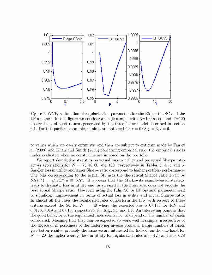
Figure 2: GCVb as function of regularization parameters for the Ridge, the SC and theLF schemes. In this �gure we consider a single sample with N=100 assets and T=120observations of asset returns generated by the three-factor model described in section6.1. For this particular sample, minima are obtained for � = 0:08; p = 3; l = 6.
to values which are overly optimistic and then are subject to criticism made by Fan etal (2009) and Khan and Smith (2008) concerning empirical risk: the empirical risk isunder evaluated when no constraints are imposed on the portfolio.We report descriptive statistics on actual loss in utility and on actual Sharpe ratio
across replications for N = 20; 40; 60 and 100 respectively in Tables 3, 4, 5 and 6.Smaller loss in utility and larger Sharpe ratio correspond to higher portfolio performance.The bias corresponding to the actual SR uses the theoretical Sharpe ratio given bySR (x�) =
p�0��1� � SR�. It appears that the Markowitz sample-based strategy
leads to dramatic loss in utility and, as stressed in the literature, does not provide thebest actual Sharpe ratio. However, using the Rdg, SC or LF optimal parameter leadto signi�cant improvement in terms of actual loss in utility and actual Sharpe ratio.In almost all the cases the regularized rules outperform the 1/N with respect to thesecriteria except the SC for N = 40 where the expected loss is 0:0188 for 1oN and0:0176; 0:019 and 0:0165 respectively for Rdg, SC and LF. An interesting point is thatthe good behavior of the regularized rules seems not to depend on the number of assetsconsidered. Meaning that they can be expected to work well in-sample, irrespective ofthe degree of ill-posedness of the underlying inverse problem. Large numbers of assetsgive better results, precisely the issue we are interested in. Indeed, on the one hand forN = 20 the higher average loss in utility for regularized rules is 0:0123 and is 0:0178
18
for 1oN; for N = 40 the higher loss in utility is 0:019 compared to 0:0188 for 1oN. Onthe other hand, for N = 60 the worst performance is 0:0077 compared to 0:0194 for1oN; for N = 100 the higher loss is obtained is 0:007 compared to 0:0202 for the naiverule. The simulations then reveal that the regularized rules proposed beat the 1oN bya larger margin for larger number of assets. The performance of the rules Rdg, SC andLF are con�rmed by the actual Sharpe ratio for which we obtain similar results.Concerning the Lasso, for all the value for N and , the regularized portfolios ob-
tained performs better than the sample-based Markowitz portfolio but is still far fromwhat is theoretically optimal. The adaptation of GCV criterion proposed by Tibshirani(1996) does not provide a good approximation to the Lasso penalty term that minimizesthe expected loss in utility, in presence of a large number of assets relative to the samplesize. The reason why this is so is that the procedure usually selects a large portion of theavailable assets, as it appears in Table 7, so that the instability of the inverse problemremains unsolved and the performance of the resulting sparse portfolio deteriorates.
6.4 Monte Carlo assessment of GCVb
A question that we seek to answer through simulations is whether the corrected versionof generalized cross-validation criterion (GCVb) provides a good approximation to thetheoretically optimal � that minimizes the expected loss in utility. To address thisissue, we use the 1000 samples generated in the previous section (T = 120 and N 2f20; 40; 60; 100g ). For each of the samples, we compute the GCVb as a function of �and determine its minimizer � . We provide some statistics for � in Table 8.To compute the MSE of � , we need to derive the true optimal regularization para-
meter � 0. To do so, we use our 1000 samples to approximate � 0 as the minimizer � 0 ofthe sample counterpart of the expected loss in utility corresponding to the use of theregularized rule bx (�) = ��1� �= :
E�(bx (�)� x�)0� (bx (�)� x�)
�where E is an average over the 1000 replications, � the theoretical covariance matrix,��1� the regularized inverse to the sample covariance matrix and x� = ��1�= thetheoretical optimal allocation. This �rst step provides us with an estimation of the trueparameter which is a function of the number of assets N and the sample size T underconsideration and does not depend on .Simulations reported in Table 8 show that the minimizer of GCVb are relatively good
approximations to the expected loss in utility of the mean-variance strategy. For eachregularization scheme the true optimal parameter is approximated by the value thatminimizes the sample counterpart of the expected loss in utility E .In general, regularization parameters have a relatively high volatility across replica-
tions especially for the LF. As this appears in the Table 8, this is mainly due to thepresence of outliers in the tails. In contrast, the value provided as a minimizer of the
19

GCVb are relatively accurate for the Rdg and SC in the sense that they are relativelyclose to the estimations of their theoretical value. A very intuitive fact concerning theridge penalty term is that it increases with the number of assets in the portfolio, re-�ecting that the penalty intensity increase with the degree of ill-posedness. In the SCcase, the GCVb criterion selects on average value of p close to 3, the number of factorsused, which is also the minimizer of the expected loss in utility in most cases.To visualize the e¤ectiveness of the regularization parameter that minimizes GCVb,
we plot in the mean-variance plane the corresponding strategies for the Rdg, the SCand the LF. All the rules are computed on a single sample of 100 asset returns andT = 120 monthly returns. A comparison is made with three benchmarks: the M, 1oNand the theoretical tangency portfolio. This experiment aims at providing a better un-derstanding of the e¤ect of regularization on the sample-based rule M. Figure 3 showshow dramatic estimation errors can a¤ect the optimality of the mean-variance opti-mizer. We can see a huge discrepancy between the theoretically optimal mean-varianceand the sample-based optimal Markowitz portfolio. However, each of our regularizedstrategies get closer to theoretically optimal rule. The main message from Figure 3 isthat regularization reduces the distance between the sample-based tangency portfolioand the theoretical tangency portfolio.
7 Empirical Application
In this section, we adopt the rolling sample approach used in MacKinlay and Pastor(2000) and in Kan and Smith (2008). Given a dataset of size T and a window sizeM , we obtain a set of T �M out-of-sample returns, each generated recursively usingthe M previous returns. For each rolling window, the portfolio constructed are held forone year (Brodie et al (2009)) which in our computations leads essentially to the sameresults as when holding optimal rules for one month (DeMiguel et al (2007, 2009)).Thetime series of out-of-sample returns obtained can then be used to compute out-of-sampleperformance for each strategy. As pointed out by Brodie et al (2009), this approach canbe seen as an investment exercise to evaluate the e¤ectiveness of an investor who baseshis strategy on the M last periods returns. For each estimation window, we minimizethe GCVb criterion to determine the optimal tuning parameter for the ridge, the spectralcut-o¤ and the Landweber-Fridman. The investment rules listed in table 2 are thencompared with respect to their out-of-sample Sharpe ratios for sub-periods extendingover M years. The obtained values re�ect the performance in terms of the reward torisk an investor would have if he were trading over the considered period.We apply our methodology to two sets of portfolios from French web site: the 48 in-
dustry portfolios (FF48) and 100 portfolios formed on size and book-to-market (FF100),ranging respectively from July 1969 to June 2009 and from July 1963 to June 2009. Fol-lowing our methodology for FF48, the optimal portfolios listed in Table 2 are constructed
20
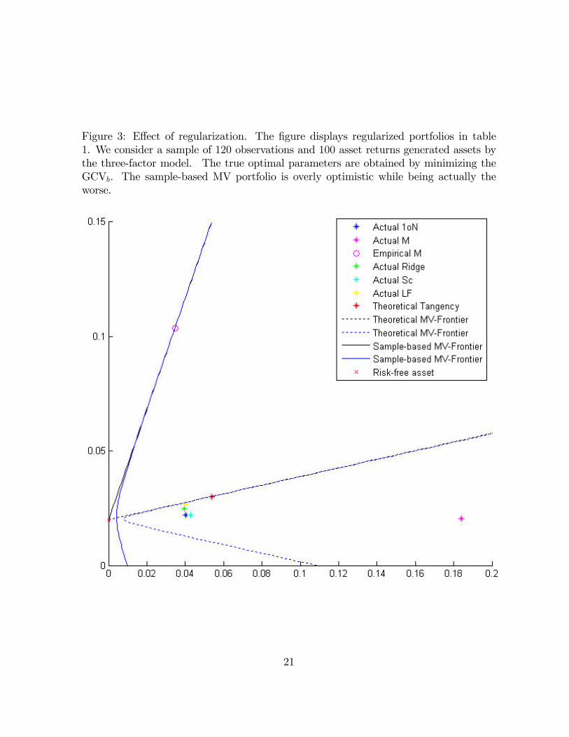
Figure 3: E¤ect of regularization. The �gure displays regularized portfolios in table1. We consider a sample of 120 observations and 100 asset returns generated assets bythe three-factor model. The true optimal parameters are obtained by minimizing theGCVb. The sample-based MV portfolio is overly optimistic while being actually theworse.
21

at the end of June every year from 1974 to 2009 for a rolling window of size M = 60months and from 1979 to 2009 for M = 120. The risk-free rate is taken to be the one-month T-bill rate. Given the estimation windows considered, the portfolio constructionproblem can be considered as ill-posed for the two datasets as re�ected by the conditionnumbers in table 11. The rolling sample covariance matrices, tend to have very smalleigenvalues and large condition numbers, and the situation is worse for the cases wherethe magnitude of N is of a comparable order of magnitude as the estimation windowM .We use an appropriate range for � to carry out our optimizations depending on the
regularization scheme. For the Ridge we use a grid on [0; 1] with a precision of 10�2,for the SC the parameter p ranges from 1 to pmax = N � 1 while for LF we use amaximal number of iterations equal to lmax = 300. For FF48 and M = 60 our �rstportfolios are constructed in June 1974. From the T � N matrix of excess returns R,empirical mean �, regularized inverse b�1� and b�� are computed using historical returnsfrom July 1969 to June 1974. We then deduce the optimal portfolio corresponding toeach type of regularization as a function of the minimizer of the corrected version ofthe GCV criterion. The portfolio obtained is kept from July 1974 to June 1975 andits returns recorded. We repeat the same process using data from July 1970 to June1975 to predict portfolio return from July 1975 to June 1976. The simulated investmentexercise is done recursively until the last set of portfolio constructed at the end of June2009. The di¤erent steps are essentially the same for the FF100 except that we onlyconsider a rolling window of M = 120; so that the �rst portfolio is constructed in June1973.In Table 12, 13, 14, we see that using a regularized portfolio is a more stable alter-
native to the Markowitz sample-based portfolio. Compared to the naive strategy, theobtained results are relatively good. The performance of the proposed rules are better inill-posed cases, (N = 48, M = 60 and N = 100, M = 120 ) where the best performanceof our regularized rule is higher than the performance the out-of-sample Sharpe ratioprovided by the 1/N rule in all the break-out periods and in the whole period of study.The lasso strategy using the approximated GCVb do not provide considerable im-
provement upon the Markowitz portfolio as noticed in the in-sample simulation exercise.E¤ort remain to be done tackle the unsatisfactory performances of the GCV-based lassoportfolio. Among possible alternatives, one that is worth investigating is a two-stageprocedure that consists in applying the Rdg, the SC or the LF scheme to subsets ofassets provided by the Lasso. Once the GCVb is minimized for each optimal subsetcontaining a given number of assets n, the open question is how do we select the opti-mal n that leads to the maximum out-of-sample performance. Table 15 that shows themaximum level of out-of-sample attainable by tuning the number of assets to be kept,after the GCV has been minimized. It supports the fact that the two-stage procedureo¤ers additional room to improvement. We plan to solve the issue in future work.
22

8 Conclusion
In this paper, we address the issue of estimation error in the framework of the mean-variance analysis. We propose to regularize the portfolio choice problem using regu-larization techniques from inverse problem literature. These regularization techniquesnamely the ridge, the spectral cut-o¤, and Landweber-Fridman involve a regularizationparameter or penalty term whose optimal value is selected to minimize the implied ex-pected loss in utility of a mean-variance investor. We show that this is equivalent toselect the penalty term as the minimizer of a bias-corrected version of the generalizedcross validation criterion.To evaluate the e¤ectiveness of our regularized rules, we did some simulations using
a three-factor model calibrated to real data and an empirical study using French�s 48industry portfolios and 100 portfolios formed on size and book-to-market. The rules areessentially compared with respect to their expected loss in utility and Sharpe ratios. Themain �nding is that in ill-posed cases a regularization to covariance matrix drasticallyimproves the performance of mean-variance problem, very often better results than theexisting asset allocation strategies and outperforms the naive portfolio especially in ill-posed cases.Our methodology can be used as well for any investment rule that requires an es-
timate of the covariance matrix and given a performance criterion. The appeal of theinvestment rules we propose is that they are easy to implement and constitute a validalternative to the existing rules in ill-posed cases, as demonstrated by our simulations.
23

Table 3: Distribution characteristics of actual loss in utility and actual Sharpe ratiofrom optimal strategies using a three-factor model for N = 20 and T = 120 over 1000replications. The risk aversion parameter is in f1; 3; 5g
Actual Loss in utility for Optimal strategies Statistics 1oN M L Rdg SC LF
Mean 0.0178 0.1516 0.0256 0.0072 0.0123 0.008Std 0.0001 0.0706 0.0705 0.0262 0.0143 0.009
= 1 q1 0.0178 0.1036 0.0056 0.0029 0.0058 0.004median 0.0178 0.1372 0.009 0.0037 0.0069 0.004q3 0.0178 0.1835 0.0155 0.0058 0.0121 0.007Mean 0.0054 0.0505 0.0085 0.0024 0.0041 0.003Std 0 0.0235 0.0235 0.0087 0.0048 0.003
= 3 q1 0.0054 0.0345 0.0019 0.001 0.0019 0.001median 0.0054 0.0457 0.003 0.0012 0.0023 0.001q3 0.0054 0.0612 0.0052 0.0019 0.004 0.002Mean 0.0032 0.0303 0.0051 0.0014 0.0025 0.002Std 0 0.0141 0.0141 0.0052 0.0029 0.002
= 5 q1 0.0032 0.0207 0.0011 0.0006 0.0012 7E-04median 0.0032 0.0274 0.0018 0.0007 0.0014 8E-04q3 0.0032 0.0367 0.0031 0.0012 0.0024 0.001
Actual Sharpe ratio for Optimal strategiesBias -0.0268 -0.1 -0.065 -0.0193 -0.0264 -0.0207Std 0 0.0537 0.0422 0.0093 0.0156 0.0095rmse 0.0268 0.1136 0.0776 0.0214 0.0307 0.0227q1 0.1533 0.0796 0.1037 0.1587 0.153 0.1579
median 0.1533 0.0942 0.12 0.1625 0.1535 0.1601q3 0.1533 0.107 0.137 0.166 0.1645 0.1634
24
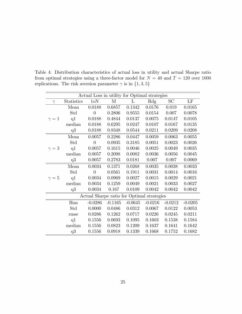
Table 4: Distribution characteristics of actual loss in utility and actual Sharpe ratiofrom optimal strategies using a three-factor model for N = 40 and T = 120 over 1000replications. The risk aversion parameter is in f1; 3; 5g
Actual Loss in utility for Optimal strategies Statistics 1oN M L Rdg SC LF
Mean 0.0188 0.6857 0.1342 0.0176 0.019 0.0165Std 0 0.2806 0.9555 0.0154 0.007 0.0078
= 1 q1 0.0188 0.4844 0.0137 0.0075 0.0147 0.0105median 0.0188 0.6295 0.0247 0.0107 0.0167 0.0135q3 0.0188 0.8348 0.0544 0.0211 0.0209 0.0208Mean 0.0057 0.2286 0.0447 0.0059 0.0063 0.0055Std 0 0.0935 0.3185 0.0051 0.0023 0.0026
= 3 q1 0.0057 0.1615 0.0046 0.0025 0.0049 0.0035median 0.0057 0.2098 0.0082 0.0036 0.0056 0.0045q3 0.0057 0.2783 0.0181 0.007 0.007 0.0069Mean 0.0034 0.1371 0.0268 0.0035 0.0038 0.0033Std 0 0.0561 0.1911 0.0031 0.0014 0.0016
= 5 q1 0.0034 0.0969 0.0027 0.0015 0.0029 0.0021median 0.0034 0.1259 0.0049 0.0021 0.0033 0.0027q3 0.0034 0.167 0.0109 0.0042 0.0042 0.0042
Actual Sharpe ratio for Optimal strategiesBias -0.0286 -0.1165 -0.0645 -0.0216 -0.0212 -0.0205Std 0.0000 0.0486 0.0312 0.0067 0.0122 0.0053rmse 0.0286 0.1262 0.0717 0.0226 0.0245 0.0211q1 0.1556 0.0693 0.1095 0.1603 0.1538 0.1584
median 0.1556 0.0823 0.1209 0.1637 0.1641 0.1642q3 0.1556 0.0918 0.1339 0.1668 0.1752 0.1682
25
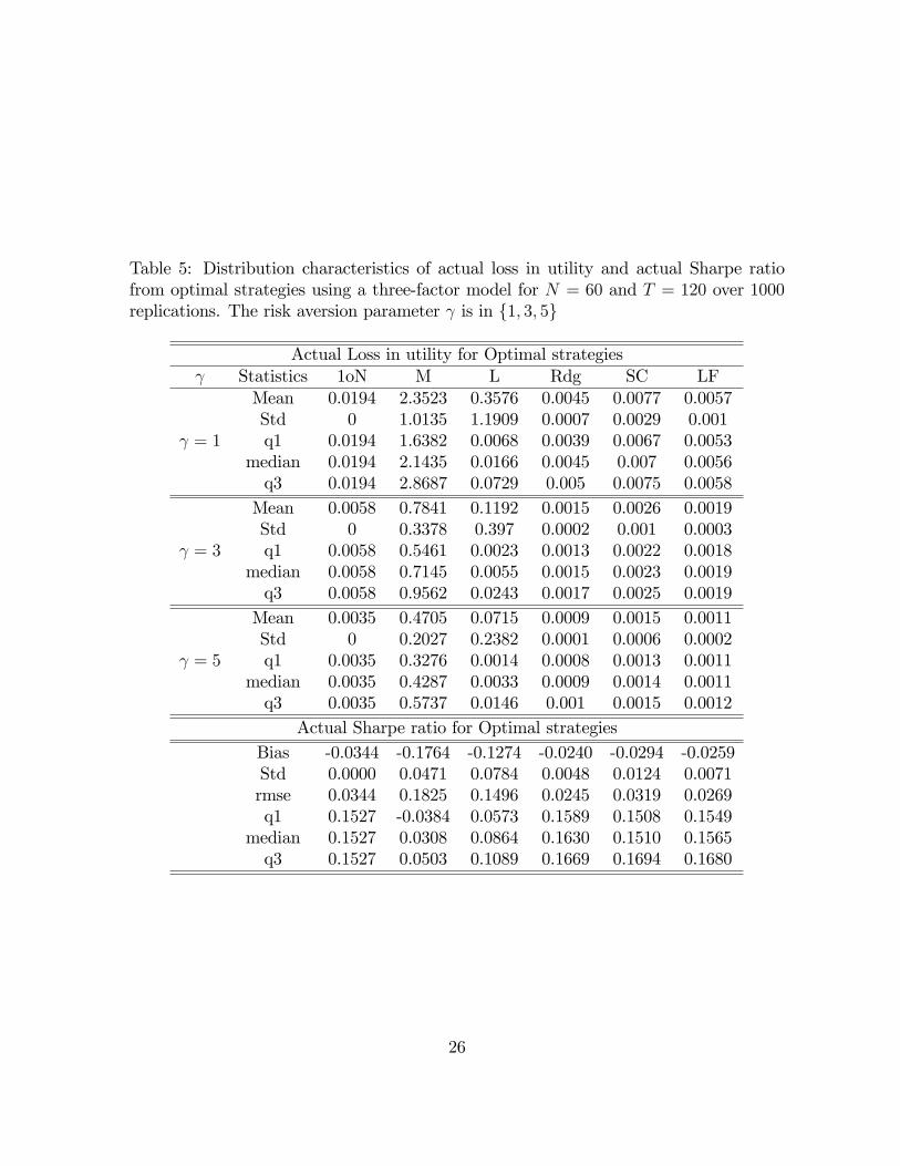
Table 5: Distribution characteristics of actual loss in utility and actual Sharpe ratiofrom optimal strategies using a three-factor model for N = 60 and T = 120 over 1000replications. The risk aversion parameter is in f1; 3; 5g
Actual Loss in utility for Optimal strategies Statistics 1oN M L Rdg SC LF
Mean 0.0194 2.3523 0.3576 0.0045 0.0077 0.0057Std 0 1.0135 1.1909 0.0007 0.0029 0.001
= 1 q1 0.0194 1.6382 0.0068 0.0039 0.0067 0.0053median 0.0194 2.1435 0.0166 0.0045 0.007 0.0056q3 0.0194 2.8687 0.0729 0.005 0.0075 0.0058Mean 0.0058 0.7841 0.1192 0.0015 0.0026 0.0019Std 0 0.3378 0.397 0.0002 0.001 0.0003
= 3 q1 0.0058 0.5461 0.0023 0.0013 0.0022 0.0018median 0.0058 0.7145 0.0055 0.0015 0.0023 0.0019q3 0.0058 0.9562 0.0243 0.0017 0.0025 0.0019Mean 0.0035 0.4705 0.0715 0.0009 0.0015 0.0011Std 0 0.2027 0.2382 0.0001 0.0006 0.0002
= 5 q1 0.0035 0.3276 0.0014 0.0008 0.0013 0.0011median 0.0035 0.4287 0.0033 0.0009 0.0014 0.0011q3 0.0035 0.5737 0.0146 0.001 0.0015 0.0012
Actual Sharpe ratio for Optimal strategiesBias -0.0344 -0.1764 -0.1274 -0.0240 -0.0294 -0.0259Std 0.0000 0.0471 0.0784 0.0048 0.0124 0.0071rmse 0.0344 0.1825 0.1496 0.0245 0.0319 0.0269q1 0.1527 -0.0384 0.0573 0.1589 0.1508 0.1549
median 0.1527 0.0308 0.0864 0.1630 0.1510 0.1565q3 0.1527 0.0503 0.1089 0.1669 0.1694 0.1680
26

Table 6: Distribution characteristics of actual loss in utility and actual Sharpe ratiofrom optimal strategies using a three-factor model for N = 100 and T = 120 over 1000replications. The risk aversion parameter is in f1; 3; 5g
Actual Loss in utility for Optimal strategies Statistics 1oN M L Rdg SC LF
Mean 0.0202 138.74 290.92 0.005 0.0038 0.0069Std 0 126.51 7799.7 0.0029 0.002 0.0026
= 1 q1 0.0202 60.586 0.0065 0.0024 0.0024 0.0038median 0.0202 98.993 0.0246 0.0032 0.003 0.0083q3 0.0202 171.42 1.6148 0.0082 0.0048 0.009Mean 0.0059 46.247 96.972 0.0017 0.0013 0.0023Std 0 42.17 2599.9 0.001 0.0007 0.0009
= 3 q1 0.0059 20.195 0.0022 0.0008 0.0008 0.0013median 0.0059 32.998 0.0082 0.0011 0.001 0.0028q3 0.0059 57.14 0.5383 0.0027 0.0016 0.003Mean 0.0036 27.748 58.183 0.001 0.0008 0.0014Std 0 25.302 1559.9 0.0006 0.0004 0.0005
= 5 q1 0.0036 12.117 0.0013 0.0005 0.0005 0.0008median 0.0036 19.799 0.0049 0.0006 0.0006 0.0017q3 0.0036 34.284 0.323 0.0016 0.001 0.0018
Actual Sharpe ratio for Optimal strategiesBias -0.0355 -0.1838 -0.1358 -0.0181 -0.021 -0.0251Std 0 0.0241 0.0584 0.0072 0.0159 0.0064rmse 0.0355 0.1853 0.1478 0.0195 0.0263 0.026q1 0.1532 -0.0127 0.0386 0.1626 0.1525 0.1584
median 0.1532 0.0057 0.0618 0.1737 0.1744 0.1593q3 0.1532 0.0228 0.0833 0.177 0.1763 0.1709
27
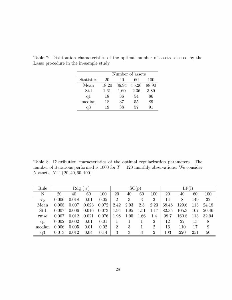
Table 7: Distribution characteristics of the optimal number of assets selected by theLasso procedure in the in-sample study
Number of assetsStatistics 20 40 60 100Mean 18.20 36.94 55.26 88.90Std 1.61 1.60 2.36 3.89q1 18 36 54 86
median 18 37 55 89q3 19 38 57 91
Table 8: Distribution characteristics of the optimal regularization parameters. Thenumber of iterations performed is 1000 for T = 120 monthly observations. We considerN assets, N 2 f20; 40; 60; 100g
Rule Rdg ( �) SC(p) LF(l)N 20 40 60 100 20 40 60 100 20 40 60 100� 0 0.006 0.018 0.01 0.05 2 3 3 3 14 8 149 32Mean 0.008 0.007 0.023 0.072 2.42 2.93 2.3 2.23 68.48 129.6 113 24.18Std 0.007 0.006 0.016 0.073 1.94 1.95 1.51 1.17 82.35 105.3 107 20.46rmse 0.007 0.012 0.021 0.076 1.98 1.95 1.66 1.4 98.7 160.8 113 32.94q1 0.002 0.002 0.01 0.01 1 1 1 2 12 22 15 8
median 0.006 0.005 0.01 0.02 2 3 1 2 16 110 17 9q3 0.013 0.012 0.04 0.14 3 3 3 2 103 220 251 50
28

Table 9: Statistical properties of the maximum eigenvalue and the minimum eigenvaluederived from the sample covariance matrices in the in-sample study
�min �maxN 20 40 60 100 20 40 60 100� 1.52E-05 2.79E-05 7.83E-06 1.53E-05 0.0346 0.0708 0.1039 0.19
Mean 1.26E-05 1.77E-05 3.80E-06 1.50E-06 0.025 0.061 0.1166 0.211Std 1.78E-06 2.75E-06 6.95E-07 3.97E-07 0.0006 0.001 0.0013 0.002q1 1.13E-05 1.58E-05 3.30E-06 1.23E-06 0.0245 0.0604 0.1157 0.209
median 1.24E-05 1.77E-05 3.76E-06 1.47E-06 0.025 0.0611 0.1166 0.211q3 1.37E-05 1.95E-05 4.26E-06 1.75E-06 0.0254 0.0617 0.1175 0.212
Table 10: Distribution characteristics of the condition number of the sample covariancematrices obtained over replications in the in-sample study.
�max=�min (�max=�min)/(�max=�min)N 20 40 60 100 20 40 60 100Mean 2027.9497 3527.8 31767.5 152232 0.8904 1.3879 2.392 12.3Std 297.58027 573.51 6058.67 47231.5 0.1307 0.2256 0.4562 3.816q1 1820.7269 3121.4 27225.8 120726 0.7994 1.228 2.05 9.753
median 2008.3814 3454.6 31054.8 143773 0.8818 1.3591 2.3384 11.61q3 2198.8976 3875.3 35266.7 171208 0.9654 1.5246 2.6555 13.83
29

Table 11: Statistics on eigenvalues and condition number of the rolling window samplecovariance matrices. The estimation window considered are M= 60, 120 and the datasetsF48 and FF100
Data set M Statistics �min �max �max=�minMean 8.93E-06 0.1197 1.77E+04Std 4.08E-06 0.0443 1.56E+04
FF48 60 q1 6.36E-06 0.0870 8.82E+03median 8.05E-06 0.1157 1.37E+04q3 1.14E-05 0.1557 2.14E+04Mean 8.58E-05 0.1160 1.68E+03Std 3.66E-05 0.0293 8.79E+02
FF48 120 q1 5.76E-05 0.0940 7.38E+02median 7.35E-05 0.1136 1.61E+03q3 0.0001237 0.1399 2.49E+03Mean 5.23E-06 0.2697 5.74E+04Std 1.52E-06 0.0645 2.78E+04
FF100 120 q1 4.14E-06 0.2265 3.79E+04median 5.07E-06 0.2527 5.14E+04q3 6.17E-06 0.3301 6.73E+04
Table 12: Out-of-sample performance in terms of Sharpe ratio of the optimal rulesapplied on FF48 using a rolling window length of 60 months.
Period 1oN M L Rdg Sc LF07/74 - 06/79 0.1334 0.0797 0.1252 0.1243 0.3006 0.262007/79 - 06/84 0.1070 -0.2879 0.0004 0.0874 -0.0186 0.122707/84 - 06/89 0.1823 0.1302 0.1895 0.2974 0.3131 0.215807/89 - 06/94 0.1077 0.0332 -0.1140 0.0490 0.2856 0.152607/94 - 06/99 0.2910 0.0433 -0.2273 0.3370 0.2954 0.337907/99 - 06/04 0.0767 0.0375 -0.0202 0.0602 0.0673 0.069907/04 - 06/09 -0.0119 -0.2494 -0.0294 -0.0212 -0.0987 -0.011107/74-06/09 0.1266 -0.0305 -0.0108 0.1334 0.1635 0.1642
30

Table 13: Out-of-sample performance in terms of Sharpe ratio of the optimal rulesapplied on FF48 using a rolling window length of 120 months. The combined rules usethe lasso a �rst step procedure and are obtained by minimizing GCV over di¤erent setsof assets.
Period 1oN M L Rdg Sc LF07/79 - 06/89 0.1468 -0.0183 0.0465 0.1311 0.1282 0.124707/89 - 06/99 0.2002 -0.0568 -0.0656 0.2427 0.1664 0.237307/99 - 06/09 0.0269 -0.0485 -0.0462 -0.0555 -0.0992 -0.046507/79 - 06/09 0.1246 -0.0412 -0.0218 0.1061 0.0651 0.1052
Table 14: Out-of-sample performance in terms of Sharpe ratio for FF100 using a rollingwindow length of M = 120 months
Period 1oN M L Rdg Sc LF07/73 - 06/83 0.1830 -0.0418 -0.1351 0.0352 0.0587 0.191707/83 - 06/93 0.1177 0.0177 0.0146 0.3083 0.3783 0.169007/93 - 06/03 0.1576 0.2848 0.3826 0.2945 0.3782 0.225107/03 - 06/09 0.0515 0.0285 -0.0877 0.0472 0.0380 0.060707/73 - 06/09 0.1275 0.0723 0.0436 0.1713 0.2133 0.1616
Table 15: Out-of-sample performance in terms of Sharpe ratio of optimal rules appliedon FF48 using a rolling window length of 60 months. The optimal number of assetsover di¤erent subsets of assets maximize the out-of-sample Sharpe ratio from holdingfor one-year the optimal rules.
Period 1oN M L Rdg Sc LF L-Rdg L-Sc L-LF07/74 - 06/79 0.1334 0.0797 0.1252 0.1287 0.3006 0.2620 0.3576 0.3506 0.362407/79 - 06/84 0.1070 -0.2879 0.0004 0.0879 -0.0186 0.1227 0.4541 0.3826 0.165307/84 - 06/89 0.1823 0.1302 0.1895 0.2979 0.3131 0.2158 0.4590 0.4937 0.376307/89 - 06/94 0.1077 0.0332 -0.1140 0.0490 0.2856 0.1526 0.2961 0.3551 0.355607/94 - 06/99 0.2910 0.0433 -0.2273 0.3372 0.2954 0.3379 0.4847 0.5193 0.486207/99 - 06/04 0.0767 0.0375 -0.0202 0.0610 0.0673 0.0699 0.2258 0.2723 0.254207/04 - 06/09 -0.0119 -0.2494 -0.0294 -0.0206 -0.0987 -0.0111 0.2369 0.3200 0.356807/69 - 06/03 0.1266 -0.0305 -0.0108 0.1344 0.1635 0.1642 0.3592 0.3848 0.3367
31

References
[1] Andrews, D. (1991) �Asymptotic optimality of generalized CL, cross-validation,and generalized cross-validation in regression with heteroskedastic errors�, Journalof Econometrics, 47, 359-377.
[2] Bai, J. and S. Ng (2008) "Forecasting economic time series using targeted predic-tors", Journal of Econometrics, 146, 304-317.
[3] Blundell, R., X. Chen, and D. Kristensen (2007) �Semi-Nonparametric IV Estima-tion of Shape-Invariant Engel Curves�, Econometrica, 75, 1613-1669.
[4] Brandt, M. W. (2004) Portfolio choice problems,http://home.uchicago.edu/lhansen/handbook.htm.
[5] Brandt, M. W., P. Santa-Clara, and R. Valkanov (2009) " Parametric PortfolioPolicies: Exploiting Characteristics in the Cross-Section of Equity Returns", Thereview of Financial Studies, 22, 3411-3447.
[6] Britten-Jones, M. (1999) �The sampling error in estimates of mean-variance e¢ cientportfolio weights�, Journal of Finance, 54, 655-671.
[7] Brodie, J., I. Daubechies, C. De Mol, D. Giannone, I. Loris (2009) �Sparse andstable Markowitz portfolios�, Proceedings of the National Academy of Sciences ofthe USA, 106, 12267-12272.
[8] Carrasco , M. (2012) �A regularization approach to the many instrument problem�,forthcoming in Journal of Econometrics.
[9] Carrasco, M., J-P. Florens (2000) �Generalization of GMM to a Continuum ofMoment Conditions�, Econometric Theory, 16, 797-834.
[10] Carrasco, M., J-P. Florens, E. Renault (2007) �Linear Inverse Problems and Struc-tural Econometrics: Estimation Based on Spectral Decomposition and Regulariza-tion�, Handbook of Econometrics, 6, 5633-5751.
[11] Craven, P. and G. Wahba (1979) �Smoothing noisy data with spline functions:Estimating the correct degree of smoothing by the method of the generalized cross-validation�, Numer. Math. 31, 377-403.
[12] DeMiguel, V., L. Garlappi, F. J. Nogales, R. Uppal (2009) �A Generalized Ap-proach to Portfolio Optimization: Improving Performance by Constraining Portfo-lio Norms�, Management Science, 55, 798-812.
32
[13] DeMiguel, V., L. Garlappi, R. Uppal (2007) �Optimal Versus Naive Diversi�cation: How Ine¢ cient is the 1/N Portfolio Strategy ? �, The review of Financial studies,22, 1915-1953.
[14] De Mol, C., D. Giannone, and L. Reichlin (2008) �Forecasting using a large numberof predictors: Is Bayesian shrinkage a valid alternative to principal components?",Journal of Econometrics, 146, 318-328.
[15] Fan, J., Y. Fan and J. Lv (2008) "High dimensional covariance matrix estimationusing a factor model", Journal of Econometrics, 147, 186-197.
[16] Fan, J., Y. Zhang and Ke Yu. (2009) "Asset allocation and Risk Assessment withGross Exposure Constraints for Vast Portfolios ", Working paper, Princeton Uni-versity.
[17] Frost, A. and E. Savarino (1986) �An Empirical Bayes Approach to E¢ cient Port-folio Selection�, Journal of Financial and Quantitative Analysis, 21, 293-305.
[18] Hoerl, A.E. and R.W. Kennard (1970) �Ridge regression: biased estimation fornonorthogonal problems�, Technometrics, 12, 55-67.
[19] Huang J., J. Horowitz, and S. Ma (2008) �Asymptotic properties of bridge es-timators in sparse high-dimensional regression models�, Annals of Statistics, 36,587-613.
[20] Jagannathan, R. and T. Ma (2003) �Risk Reduction in Large Portfolios: WhyImposing the Wrong Constraints Helps�, Journal of Finance, LVIII, 1651-1683.
[21] Jobson, J.D. and B. Korkie (1983) �Statistical Inference in Two-Parameter PortfolioTheory with Multiple Regression Software�, Journal of Financial and QuantitativeAnalysis, 18, 189-197.
[22] Kan, R. and D. R. Smith (2008) " The distribution of the Sample Minimun-VarianceFrontier", Management, 54, 1364-1380.
[23] Kan, R. and G. Zhou (2007) "Optimal portfolio choice with parameter uncertainty",Journal of Financial and Quantitative Analysis, 42, 621-656.
[24] Ledoit, O. and M. Wolf (2003) �Improved estimation of the covariance matrix ofstock returns with an application to portfolio selection�, The Journal of EmpiricalFinance, 10, 603-621.
[25] Ledoit, O. and M. Wolf (2004a) �Honey, I shrunk the sample covariance matrix�,The Journal of Portfolio Management, 30, 110-119.
33

[26] Ledoit, O. and M. Wolf (2004b) � A Well-Conditioned Estimator for Large-Dimensional Covariance Matrices�, Journal of Multivariate Analysis, 88, 365-411.
[27] Li, K.C. (1986) �Asymptotic optimality of CL and generalized cross-validation inridge regression with application to spline smoothing�, The Annals of Statistics,14, 1101-1112.
[28] Li, K-C. (1987) �Asymptotic optimality for Cp, CL, cross-validation and generalizedcross-validation: Discrete Index Set�, The Annals of Statistics, 15, 958-975.
[29] MacKinlay, A.C. and L. Pastor (2000) �Asset Pricing Models: Implications forExpected Returns and Portfolio Selection�, The Review of �nancial studies, 13,883-916.
[30] Markowitz, H. M. (1952) �Portfolio selection�, The Journal of Finance, 7, 77-91.
[31] Michaud, R.O. (1989) �The Markowitz Optimization Enigma: Is Optimal Opti-mized�, Financial Analyst Journal, 45, 31-42.
[32] Prigent, J.-L. (2007) Portfolio Optimization and performance analysis, Chapmanand Hall/CRC.
[33] Stock, J. and M. Watson (2002) "Forecasting Using Principal Components from aLarge Number of Predictors", Journal of the American Statistical Association, 97,1167-1179.
[34] Tibshirani, R. (1996) �Regression Shrinkage and Selection via the Lasso �J. Roy.Statist. Soc. B, 58, 267-288.
[35] Tu, J. and G. Zhou (2010) � Markowitz Meets Talmud: A combination of Sophis-ticated and Naive Diversi�cation Strategies�, Journal of Financial Economics, 99,204-215.
[36] Varian, H. (1996) �A Portfolio of Nobel Laureates: Markovitz, Miller and Sharpe�, The Journal of economic Perspectives, 7, 159-169.
[37] Whittle, P. (1960) "Bounds for the moments of linear and quadratic forms in inde-pendent variables", Theory Probab. Appli. 5, 302-305.
34

Appendix A: Homotopy - LARS Algorithms for penalized least-squaresHomotopy (Continuation) is a general approach for solving a system of equation by
tracking the solution of nearby system of parametrized equation. In the penalized Lassocase the Homotopy variable is the penalty term. We give below a detailed descriptionof the Homotopy/LARS algorithm which provides the solution path to the l1-penalizedleast-squares objective function:
~x(�) = argminxky �Rxk22 + � kxk1 :
The solution to this minimization problem ~x(�) is provided as a continuous piecewisefunction of the penalty � satisfying the variational equations given by:�
(R0(y �Rx))i =�2sgn(xi) xi 6= 0
j(R0(y �Rx))ij � �2
xi = 0
Meaning that the residual correlations bi = (R0(y �Rx))i corresponding to nonzero weights are equal to �=2 in absolute value, while the absolute residual correla-tion corresponding the zero weights must by bounded by �=2. Throughout the al-gorithm, it is critical to identify the set of active elements, that is the componentswith non zeros weights. At a given iteration k of the algorithm this set is denoted byJk =
ni for which jbij = �k
2
o, and also corresponds to the set of maximal residual cor-
relations components.
The algorithm starts with an initial solution satisfying the variational equations,for a penalty term suitably chosen. The obvious initial solution is obtained by settingall the weights to zeros. The corresponding penalty term � 0, must then satisfy � 0 �2maxi j(R0y)ij. Hence we have that ~x(�) = 0 for all � � � 0. This allow us to setJ1 = fi�g, where i� = argmaxi j(R0y)ij.From one iteration k to the next the algorithm manages to update the active set
Jk, which represents the support of ~x(� k), so that the �rst-order conditions remainssatis�ed. Hence in each iteration k + 1, the vector b decreases at the same rate k+1 inthe active set to preserve the same level of correlation for active elements.
(bk+1)Jk+1 = (bk)Jk+1 � k+1(sign(bk))Jk+1
This result is obtained by updating the optimal weights while moving along a walkingdirection uk+1:
x(� k+1) = x(� k) + k+1uk+1
Denote RJ the submatrix consisting of the columns J of R, the walking directionun+1 is a solution to a linear system:
R0Jk+1RJk+1(uk+1)Jk+1 = (sgn(b
k)Jk+1) =�sgn(bkj )j2Jk+1
�= vk+1
35

The remaining components of uk+1 are set to zero that is:
uk+1i = 0 for i =2 Jk+1
The step k+1 to make in direction uk+1 to �nd x(� k+1) is the minimum value such
that an inactive element becomes active or the reverse.If an inactive element i becomes active, it means that its correlation reached the
maximal correlation in the descent procedure. And then is must be case that:
��bki � k+1r0k+1i
�� = ��(bk)Jk+1 � k+1vJk+1�� = � k+1 =
� k
2� k+1
with ri is the ith column of R. This implies that:
k+1 =�k
2� bki
1� r0k+1i
or n+1 =�k
2+ bki
1 + r0k+1i
The optimal step is then given by :
k+1+ = mini2Jc
+
(�k
2� bki
1� r0k+1i
;�k
2+ bki
1 + r0k+1i
)
On the other hand, if n+1 is such that an active element i reaches zero then (??)implies that:
k+1� = � xkiuk+1i
The smallest step to make so that an element leaves the active set:
k+1� = mini2Jk+1
+
�� xkiuk+1i
�Finally the next step is given by:
k+1 = min� k+1+ ; k+1�
At the end of each stage the corresponding penalty term is � k+1 = � k � 2 k+1 which
is smaller than � k. We stop when � k+1 becomes negative. After q + 1 iterations theAlgorithm provides q + 1 breakpoints � 0 > � 1 > � � � > � q and their correspondingminimizers x(� i). From there, the optimal solution for any � can be deduced by linearinterpolation.
36
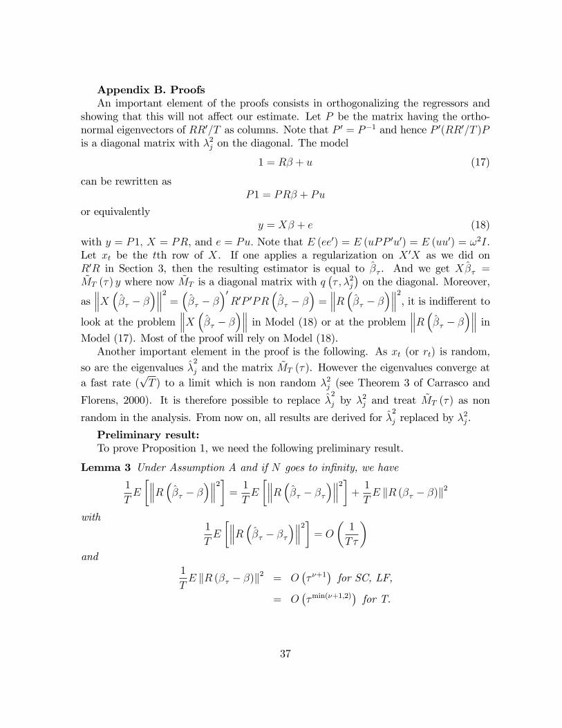
Appendix B. ProofsAn important element of the proofs consists in orthogonalizing the regressors and
showing that this will not a¤ect our estimate. Let P be the matrix having the ortho-normal eigenvectors of RR0=T as columns. Note that P 0 = P�1 and hence P 0(RR0=T )Pis a diagonal matrix with �2j on the diagonal. The model
1 = R� + u (17)
can be rewritten asP1 = PR� + Pu
or equivalentlyy = X� + e (18)
with y = P1; X = PR, and e = Pu: Note that E (ee0) = E (uPP 0u0) = E (uu0) = !2I.Let xt be the tth row of X. If one applies a regularization on X 0X as we did onR0R in Section 3, then the resulting estimator is equal to �� . And we get X�� =~MT (�) y where now ~MT is a diagonal matrix with q
�� ; �2j
�on the diagonal. Moreover,
as X ��� � �
� 2 = ��� � ��0R0P 0PR
��� � �
�= R��� � �
� 2, it is indi¤erent tolook at the problem
X ��� � �� in Model (18) or at the problem R��� � �
� inModel (17). Most of the proof will rely on Model (18).Another important element in the proof is the following. As xt (or rt) is random,
so are the eigenvalues �2
j and the matrix ~MT (�). However the eigenvalues converge ata fast rate (
pT ) to a limit which is non random �2j (see Theorem 3 of Carrasco and
Florens, 2000). It is therefore possible to replace �2
j by �2j and treat ~MT (�) as non
random in the analysis. From now on, all results are derived for �2
j replaced by �2j .
Preliminary result:To prove Proposition 1, we need the following preliminary result.
Lemma 3 Under Assumption A and if N goes to in�nity, we have
1
TE
� R��� � �� 2� = 1
TE
� R��� � ��
� 2�+ 1
TE kR (�� � �)k2
with1
TE
� R��� � ��
� 2� = O
�1
T�
�and
1
TE kR (�� � �)k2 = O
�� �+1
�for SC, LF,
= O��min(�+1;2)
�for T.
37

In summary1
TE R��� � �
� 2 � �21
T�+ C� �+1
which is minimized for � = T�1=(�+2) and is equivalent to T�(�+1)=(�+2). We can check
that Li (1986)�s condition for optimality holds, namely that inf�E R��� � �
� 2 !1.Note that if N is �xed, this condition is not ful�lled.
Proof of Lemma 3. As discussed earlier, it is indi¤erent to work on X ��� � �
� in Model (18) or on
R��� � �� in Model (17). From now on, we work with Model
(18): y = X� + e: We have Xb�� = ~MT (�) y and E�Xb�� jX� � X�� = ~MT (�)X�
where E (:jX) denotes the linear projection on X. Hence,
X�b�� � ��
�= ~MT (�) e;
X (�� � �) =�~MT (�)� IT
�X�:
The �rst equality in Lemma 3 follows from the fact that the cross-product vanishes,indeed:
EDX�b�� � ��
�; X (�� � �)
E=Xj
qj (1� qj)E�ejx
0j��= 0;
where qj denotes q�� ; �2j
�.
E X �b�� � ��
� 2 = E�e0 ~MT (�)
2 e�
= !2Xj
q�� ; �2j
�2� !2 sup q
�� ; �2j
�Xj
q�� ; �2j
�= O
�1
�
�
38

by Lemma 4 of Carrasco (2012). We have
1
TkX (�� � �)k2 =
1
T
� ~MT (�)� IT
�X� 2
=Xj
(qj � 1)2hX�; vji2
T
=Xj
�2j (qj � 1)2D�; �j
E2
=Xj
�2+2�j (qj � 1)2D�; �j
E2�2�j
� sup�2+2�j (qj � 1)2Xj
D�; �j
E2�2�j
:
Taking the expectation, one obtains
1
TE kX (�� � �)k2 � sup�2+2�j (qj � 1)2
Xj
�; �j
�2�2�j
=
�O�� (�+1)
�for SC and LF,
O��min(�+1;2)
�for Ridge
by Assumption A and Proposition 3.11 of Carrasco, Florens, and Renault (2007).
Proof of Proposition 1.First we analyze the elements of (12):
�� (�0�)� �
��0��
�=
��� � �
�(�0�)� �
��0�� � �0
�� � �� + ��
��=
��� � �
�(�0�)� �
�(�� �)0 �� + �0
��� � �
��=
��� � �
��0�| {z }
(a1)
� � (�� �)0��� � �
�| {z }
(a2)
� � (�� �)0 �| {z }(a3)
� ��0��� � �
�| {z }
(a4)
: (19)
Term (a2):���(�� �)0
��� � �
����2 � k�� �k2 �� � �
2 = Op�NT
� �� � � 2 :
Term (a3):��(�� �)0 �
��2 � k�� �k2 k�k2 = Op�NT
�because k�k2 <1:
So both terms (a2) and (a3) will be negligible compared to �� � �
2 by AssumptionB(iv) and Lemma 3.
39

1�1� �0��
� � 1
1� �' 1
1� �+
1
(1� �)2
�� � �
�
=1
1� �0�+�0��� � �
�(1� �0�)2
+ o��0��� � �
��:
Since �0��� � �
�= op (1), we have
�� � ��1� �0��
� = �� � �
(1� �0�)+Op
���� � �
��0��� � �
��:
��� � �
�0���� � �
�=
��� � �
�0���� � �
�+��� � �
�0 ��� �
���� � �
�:
Moreover, ��� � �
�0 ��� �
���� � �
��
�� � � 2 �� �
= Op
�1pT
�� � � 2�
by Theorem 4 of Carrasco and Florens (2000) and the Hilbert-Schmidt assumption of�. �
�� � ��0���� � �
�=
��� � �
�0 �R0RT
��R01
T
��R01
T
�0���� � �
�+Op
0B@ �� � �
2pT
1CA=
1
T
��� � �
�0R0R
��� � �
����� � �
�0��0��� � �
�+Op
0B@ �� � �
2pT
1CA=
1
T
R��� � �� 2 � ��0 ��� � �
��2+Op
0B@ �� � �
2pT
1CA :
40

Using (12) and (19), we obtain
(x� � x�) =
��� � �
�(1� �0�)
+��0
��� � �
�(1� �0�)2
+Op
���� � �
��0��� � �
��+Op
rN
T
!:
(x� � x�)0� (x� � x�) (20)
=
��� � �
�0���� � �
�(1� �0�)2
+
��� � �
�0��0���0
��� � �
�(1� �0�)4
+2
��� � �
�0���0
��� � �
�(1� �0�)3
+Op
���� � �
�0���� � �
��0��� � �
��+ op
rN
T���� � �
�!:
41
Replacing � by R0R=T � ��0, (20) is equal to
1T
R��� � �� 2
(1� �0�)2(21)
�
��0��� � �
��2(1� �0�)2
(22)
+1
T
R��0 ��� � �� 2
(1� �0�)4(23)
�
�b�0��0 ��� � ���2
(1� �0�)4(24)
+2
T
��� � �
�0R0R��0
��� � �
�(1� �0�)3
(25)
�2
��� � �
�0 b� �b�0���0 ��� � ��
(1� �0�)3(26)
+rest (�) : (27)
Note that b�0� is a scalar that can be approximated by �0�. The next step consists intaking the expectation of each term and writing �� � � = �� � �� + �� � �:
42

We turn our attention to E���0��� � �
��2�. The variance term is given by
1
T 2E
���0��� � ��
��2�=
1
T 2E
"�10TTR��� � ��
��2#
=1
T 2E
"�10TTMT (�) e
�2#
=1
T 2E
�e0MT (�)
1T10T
T 2MT (�) e
�=
1
T 2E
��Xqjej
�2�=
Pq2j!
2
T 2+1
T 2
Xj
Xi6=j
qjqi!2
�Pq2j!
2
T 2+!2
T 2
Xj
qjXi
qi (28)
� 1
T 2E R��� � ��
� 2 +O
�1
� 2T 2
�: (29)
Therefore, this term is negligible with respect to (21). However, the bias term is not:
(�0 (�� � �))2=
�10TT(MT (�)� IT )R�
�2� k1Tk2
T 2k(MT (�)� IT )R�k2
� 1
Tk(MT (�)� IT )R�k2 :
Therefore, the bias of (22) may be of the same order as that of (21).Let us examine the term (23):The variance corresponding to (23) is
1
TE
���� � ��
�0��0R0R��0
��� � ��
��Note that R
0RT� = R0R
TE�R0RT
��1� ' �: Replacing � by �, we get
1
TE
���� � ��
�0��0R0R��0
��� � ��
��' �0�E
���0��� � ��
��2�43

which is negligible.The bias corresponding to (23) is
(�� � �)0 ��0R0RT��0 (�� � �)
(1� �0�)4
' �0�(�0 (�� � �))2
(1� �0�)4:
Similarly, the variances of the terms (24) to (26) are negligible. The bias termcorresponding to (24) is equal to
��b�0��0 (�� � �)
�2(1� �0�)4
' �(�0�)2 (�0 (�� � �))2
(1� �0�)4:
Combining the biases of (23) and (24), we obtain
(�0�) (�0 (�� � �))2
(1� �0�)3:
The bias corresponding to the term (25) is given by
2(�� � �)0 R
0RT��0 (�� � �)
(1� �0�)3
' 2(�0 (�� � �))2
(1� �0�)3:
The bias term corresponding to (26) is equal to
�2(�� � �)0 b� �b�0���0 (�� � �)
(1� �0�)3
' �2(�0�) (�0 (�� � �))2
(1� �0�)3:
Combining the bias terms of (22) to (26), we obtain
(�0�) (�0 (�� � �))2
(1� �0�)3+(�0 (�� � �))2
(1� �0�)2
=(�0 (�� � �))2
(1� �0�)3:
44
Combining all the terms together, we obtain:
2 (1� �0�)2E�(x� � x�)0� (x� � x�)
�=
1
TE R��� � �
� 2 + (�0 (�� � �))2
(1� �0�)+ rest (�) :
Proof of Proposition 2.Intermediate result: Let = E (xtx
0t) = E (X 0X) =T = E (R0R) =T:
R�T (�) =1
TE X� �Xb�� 2 + (15)
=1
T
Xj
(1� qj)2 (�0�) +
!2
T
Xj
q2j + (15) (30)
where !2 = E�e2j�:
Proof of (30): Let AT (�) = I �MT (�). Following the proof of Li (1987), we have
1
TE X� �Xb�� 2
=1
TE kX� �MT (�) (X� + e)k2
=1
TE kAT (�)X� �MT (�) ek2
=1
TkAT (�)X�k2 +
1
TE kMT (�) ek2 +
2
TE [hAT (�)X�;MT (�) ei] :
As MT (�) and AT (�) are diagonal matrices, we have
1
TkAT (�)X�k2 =
1
T
Xj
(1� qj)2Eh�x0j��2i
=1
T
Xj
(1� qj)2 (�0T�) ;
where �0T� = �0� < 1;
E hAT (�)X�;MT (�) ei =Xj
qj (1� qj)E�ejx
0j��= 0
and E�kMT (�) ek2
�= E
�Pj q
2j e2j
�= !2
Pj q
2j :
45

First we establish the optimality for a Mallows�CL criterion where !2 is assumed tobe known. Let
�C = argmin�fCrit (�)g
whereCrit (�) =
1
Tk(IT �MT (�)) yk+ 2!2
1
TtrMT (�) + (15)
We want to show thatLT (�C)
inf� LT (�)
P! 1: (31)
Crit (�) can be rewritten as
Crit (�)
=1
Tkek2 + LT (�) +
2
The; AT (�)X�i
+2
T
�!2trMT (�)� he;MT (�) ei
�+(15)� (�
0 (�� � �))2
1� �0�
�rest (�) :
To establish (31), we need to show that in probability
Crit (�)� cT = LT (�) (1 + "T (�))
wheresup�j"T (�)j = op (1) :
Hence, to establish (31), it is su¢ cient to show that
sup�
�� 1The; AT (�)X�i
��R�T (�)
! 0; (32)
sup�
1Tj!2trMT (�)� he;MT (�) eij
R�T (�)! 0 (33)
sup�
jrest (�)jR�T (�)
! 0; (34)
sup�
�����(15)� (�0 (�� � �))2
1� �0�
����� =R�T (�) ! 0; (35)
sup�
����LT (�)R�T (�)� 1���� ! 0 (36)
46
Proof of the optimality of Mallows�CL criterion for SC and LF:Now we focus to the case of SC and LF regularizations. By a slight abuse of notation,
� denotes from now on the number of eigenvalues retained in SC or the number ofiterations in LF. Note that � is an integer number and lies in a discrete index setHT = f1; 2; :::; Ng for SC since N � T and HT = f1; 2; :::; Tg for LF. We are going tocheck the conditions (32) to (36). We follow a proof similar to that of Li (1987).Consider (32). By Chebyshev�s inequality, we have
P
"sup�2HT
�� 1The; AT (�)X�i
��R�T (�)
> �
#�X�2HT
1T 2m
E�he; AT (�)X�i2m
��2mR�T (�)
2m (37)
for some integer m: Using the fact that AT (�) is diagonal, we have
E�he; AT (�)X�i2m
�= E
24 Xj
ej (1� qj)x0j�
!2m35< C
Xj
E��ejx
0j��2m�1=m
(1� qj)2
!m
for some constant C by Theorem 2 of Whittle (1960) using the fact that ejx0j� areindependent and have mean zero (which follows from rt; ut i.i.d. and E (utrt) = 0).Moreover, Lp inequality implies that
1
T
Xj
E��ejx
0j��2m�1=m
(1� qj)2 � 1
T
Xj
E��ejx
0j��2�
(1� qj)2
� C1
T�0T�
Xj
(1� qj)2 (38)
� CR�T (�)
where inequality (38) follows from the fact that et = yt � x0t� and e0X� =
Pt etx
0t�.
Moreover as etx0t� are independent with mean zero, we have
E�(etx
0t�)
2�= E
(e0X�)2
T
!= E
(u0R�)2
T
!= E
�(utr
0t�)
2�:
Now replacing ut by 1� r0t�, we obtain
E�(utr
0t�)
2�� E
�(r0t�)
2�+ E
�(r0t�)
4�< CE
�(r0t�)
2�
where C can be taken equal to 2�E�(r0t�)
2�+ E�(r0t�)
4�� =E �(r0t�)2� :47

Therefore, (37) is no greater than C��2mP
�2HT (TR�T (�))
�m which tends to zeroby assumption B3.Now, consider (33),
!2trMT (�)� he;MT (�) ei =Xj
�!2 � e2j
�qj:
Again by Chebyshev�s inequality,
P
�sup�
1Tj!2trMT (�)� he;MT (�) eij
R�T (�)> �
��X�
1T 2m
E
��Pj
�!2 � e2j
�qj
�2m�R�T (�)
2m :
By Whittle (1960, Theorem 2), we have
1
T 2mE
24 Xt
�!2 � e2t
�qt
!2m35 � C1
T 2m
Xj
q2jE��!2 � e2j
�2m�1=m!m
� C 01
T 2m
Xj
q2j
!m� C 0
1
TmR�T (�) :
Hence, (33) holds by Assumption B3.Consider (35). Using � = �� �+ �, we have
(15)� (�0 (�� � �))2
1� �0�
= (15)� (�0 (�� � �))
2
1� �0���(�� �)0 (�� � �)
�21� �0�
� �0 (�� � �) (�� �)0 (�� � �)
1� �0�
Note that b�0 (�� � �) =10T (MT (�)�IT )R�
Tand�
10T (MT (�)� IT )R��2
T 2�1� b�0b�� =
�10T (MT (�)� IT )R�
�2T 2 (1� �0�)
+
�10T (MT (�)� IT )R�
�2T 2 (1� �0�)2
��0� � b�0b�� :
48

Moreover, ��������10T (MT (�)� IT )R�
�2T 2
��b�0 (�� � �)
�2�������=
������10T (MT (�)� IT )R
�� � �
�T
10T (MT (�)� IT )R�� + �
�T
������� k10T (MT (�)� IT )k2
T
R�� � ��
pT
R�� + ��
pT
=Xj
(qj � 1)2
Top (1)
� CR�T (�) op (1)
because R�� + �
� 2 =T = �� + ��0(Prtr
0t=T )
�� + �
�<1 because �0T� < 1:
Consider (36). Given LT = L�T + rest and (34) holds, it su¢ ces to prove the resultfor L�T instead of LT : Let d (�) denote (�
0 (�� � �))2 =(1� �0�).
L�T (�) =1
T
X ��� � �� 2 + d (�)
=1
TkAT (�)X� �MT (�) ek2 + d (�)
=1
TkAT (�)X�k2 +
1
TkMT (�) ek2 �
2
ThAT (�)X�;MT (�) ei+ d (�) :
L�T (�)�R�T (�) =1
T
�kMT (�) ek2 � E
�kMT (�) ek2
��� 2ThAT (�)X�;MT (�) ei :
Hence, we need to show that
sup�
1TjhAT (�)X�;MT (�) eij
R�T (�)! 0; (39)
sup�
1T
�kMT (�) ek2 � E
�kMT (�) ek2
��R�T (�)
! 0: (40)
Note that jhAT (�)X�;MT (�) eij =���Pj qj (1� qj)x
0j�ej
��� � ���Pj (1� qj)x0j�ej
��� be-cause sup jqj � 1. Similarly,
��kMT (�) ek2 � E�kMT (�) ek2
��� = ���Pj
�!2 � e2j
�q2j
��� �49

���Pj
�!2 � e2j
�qj
���. So the same proof as for (32) and (33) can be used to establish (39)and (40).This completes the proof of the optimality of Mallows�CL criterion for SC and LF.
Relating the GCV to the CL via the Nil trace estimator:Denote T = X� and T = MT (�) yT .
The GCV can be related to CL via the nil-trace estimate, de�ned from the estimateof interest T as
� T = ��yT + (1 + �) T
with
� =n�1trMT (�)
1� n�1trMT (�)
In other words, � T = �MT (�) yT with
�MT (�) = ��I + (1 + �)MT (�)
From the previous expression, tr �MT (�) = 0. Then selecting a model from the classf T (�) : � 2 HT g using the GCV criterion, is equivalent to using the CL to select anestimate from f� T (�) : � 2 HT g. Following Li 87, we adopt the following assumptions:
Assumption CA4: inf
h2HTLT (�)! 0
A5: for any f�T 2 HTg such that : T�1trMT (�)MT (�)0 ! 0
we have (T�1trMT (�))2
T�1trMT (�)MT (�)0 ! 0
A6: suph2HT
T�1trMT (�) � 1 for some 1 > 1 > 0
A7: suph2HT
(T�1trMT (�))2
T�1trMT (�)MT (�)0 � 2 for some 1 > 2 > 0
Under assumption A1-A7, the crucial inequality (6.3 and 6.4 in Li, 87)
c1 �tr �MT (h) �MT (h)
0
trMT (h)MT (h)0 � c2; c1 �
�RT (h)
RT (h)� c2;
where c1 and c2 are two positive constants, still hold. The justi�cation of the replacementof the original estimate by the nil-trace estimate is then essentially the same as in Li87, Theorem 3.2.Let us check that the assumption C is satis�ed for SC. A4 is implied by Lemma 3
in Appendix. Then note that
T�1trMT (�)MT (�)0 =
1
T
Xj
qj =1
T�=N�T
50

where N� is the number of selected eigenvectors. A5 is trivially satis�ed. A6 and A7are equivalent to
N�T
< 1: (41)
Given that N� is necessarily smaller than N (the number of assets) and N is limited byassumption B(iv), condition (41) holds. The asymptotic optimality of SC follows.
51