Optimal Pilot Placement for Time-Varying Channels fileoutperforms RPP-1 in the other regimes. This demonstrates the potential for using superimposed training This demonstrates the

1

ADAPTIVE COMMUNICATIONS AND SIGNAL PROCESSING LABORATORY

CORNELL UNIVERSITY, ITHACA, NY 14853

Optimal Pilot Placement for Time-Varying Channels

Min Dong, Lang Tong and Brian M. Sadler

Technical Report No. ACSP-TR-01-03-02

January 2003

January 29, 2003 DRAFT

2

Abstract

Two major training techniques for wireless channels are time division multiplexed (TDM) training

and superimposed training. For the TDM schemes with regular periodic placements (RPP), the closed-

form expression for the steady-state minimum mean square error (MMSE) of channel estimate is obtained

as a function of placement for Gauss-Markov flat fading channels. We then show that, among all periodic

placements, the single pilot RPP scheme (RPP-1) minimizes the maximum steady-state channel MMSE.

For BPSK and QPSK signaling, we further show that the optimal placement that minimizes the maximum

bit error rate (BER) is also RPP-1. We next compare the MMSE and BER performance under the

superimposed training scheme with those under the optimal TDM scheme. It is shown that while the

RPP-1 scheme performs better at high SNR and for slowly varying channels, the superimposed scheme

outperforms RPP-1 in the other regimes. This demonstrates the potential for using superimposed training

in relatively fast time-varying environments.

Index Terms

Time Varying, Channel Tracking, Gauss-Markov, Kalman Filter, Pilot Symbols, Placement Schemes,

PSAM, Superimposed.

EDICS: 3-CEQU (Channel modeling, estimation, and equalization), 3-PERF (Performance Anal-

ysis, Optimization, and Limits).

I. INTRODUCTION

Channel estimation is a major challenge for reliable wireless transmissions. Often, in practice,

pilot symbols known to the receiver are multiplexed with data symbols for channel acquisition.

Two major types of training for single carrier systems are time division multiplexed (TDM)

training, and superimposed training. Pilot symbols in a TDM system are inserted into the data

stream according to a certain placement pattern, and the channel estimate is updated using these

pilot symbols. For superimposed training, on the other hand, pilot and data symbols are added

and transmitted together, and the channel estimate is updated at each symbol.

The way that pilot symbols are multiplexed into the data stream affects the system performance

for time-varying channels. Under TDM training, the presence of pilot symbols makes channel

estimation accurate at some periods of time and coarse at others. If the percentage of pilot

symbols is fixed, we then have to choose between obtaining accurate estimations infrequently,

or frequent but less accurate estimates. Is it better to cluster pilot symbols as in the case of GSM

DRAFT January 29, 2003

3

systems, or to spread pilot symbols evenly in the data stream as in the pilot symbol assisted

modulation (PSAM) [1]? What is the optimal placement that minimizes the mean square error

(MSE) of the channel estimator? Does the MSE-minimizing training also minimize the bit error

rate (BER)? In choosing the optimal training scheme, do we need to know the rate of channel

variation and the level of signal-to-noise ratio (SNR)? How does TDM training compare with

superimposed training? Intuitively, superimposed training may have the advantage when the

channel fades rapidly, but the superimposed data interferes with pilot-aided channel estimation,

which may lead to an undesirable performance floor in the high SNR regime.

In this paper, we address these issues systematically. We model the time-varying flat fading

channel by a Gauss-Markov process, and use the minimum mean square error (MMSE) channel

estimator along with the symbol-by-symbol maximum likelihood (ML) detector. The MMSE

channel estimator is implemented using the Kalman filter. For TDM training we show that, among

all periodic placements, the regular periodic placement with pilot cluster size one (referred to as

RPP-1) minimizes the maximum steady-state channel MMSE and BER for both BPSK and QPSK

signaling, regardless of the SNR level or the rate of channel variation. Given the constraint of the

minimum length of pilot clusters � , we show that RPP- � is optimal. Performance comparisons

between the optimal TDM scheme and the superimposed scheme are given both analytically

and numerically. We show that the optimal TDM scheme performs better at high SNR and for

slowly varying channels, whereas the superimposed scheme is superior for many situations of

practical importance. In the process of establishing the optimality of RPP-1, we also provide the

closed-form expression for steady-state channel MMSE at each data symbol position, which is

useful to evaluate the performance of coded transmissions.

Pilot symbol assisted modulation (PSAM), proposed in [2], [3], includes the periodic TDM

training with cluster size one—the RPP-1 scheme. Cavers first analyzed the performance of

PSAM [1]. While the optimality of RPP-1 has never been shown for either channel MMSE

or BER until now, it has been applied and studied in various settings [4]–[8]. The optimality

of RPP-1 may not be surprising in retrospect–but that the optimality holds uniformly across all

fading and SNR levels may seem unexpected. Establishing the optimality formally and uniformly

across a wide range of channel conditions, however, does not come from a direct application

of the standard Kalman filtering theory. In particular, we need to examine all possible training

patterns and their corresponding maximum steady-state MMSEs, which would not have been


4

possible without characterizing the MSE behavior with respect to the placement pattern. Under

TDM training, the channel estimator switches between the Kalman updates using pilot symbols

and the Kalman predictions during data transmissions, and the switching occurs before the

steady-state in either phase has been reached.

Optimal training has been previously considered for block fading channels from a channel

estimation perspective under both TDM and superimposed trainings [9]–[11], and from an

information theoretic viewpoint [12], [13]. For time-varying channels, existing results tend

to assume the RPP-1 scheme and optimize parameters such as pilot symbol spacing, power

and rate allocations [1], [6], [7]. In [6], for flat Rayleigh fading modeled by a Gauss-Markov

process and the PSAM scheme, the optimal spacing between the pilot symbols is determined

numerically by maximizing the mutual information with binary inputs. In [7], with the flat fading

channel modeled by a band-limited process, at high SNR and large block length regime, optimal

parameters for pilots, including pilot symbol spacing and power allocation, are determined by

maximizing a lower bound on capacity. In [14], the performance in various aspects of CDMA

systems under two pilot-assisted schemes is analyzed. In [15], we addressed the problem of

optimal placement of pilot symbols in TDM schemes for packetized transmission over time

varying channels at high SNR.

This paper is organized as follows. In Section II, we study the optimal pilot placement

for TDM schemes. We first introduce the system model and formulate the problem, and then

obtain the optimal placement for both channel tracking and BER performance. We then consider

superimposed training in Section III, where we derive the steady-state channel MSE with Kalman

tracking, and the BER. In Section IV, we provide both analytical and numerical performance

comparison under the optimal TDM scheme, and the superimposed scheme. Finally, we conclude

in Section V.

II. OPTIMAL PLACEMENT FOR TDM TRAINING

A. The Channel Model

We model a time-varying flat Rayleigh fading channel as

�� (1)


5

where �� is the received observation, � � the transmitted symbol, �� the zero mean

complex Gaussian channel state with variance � , and �� the complex circular

AWGN at time � . We assume that data � � , channel �� , and noise �� are jointly independent.

The dynamics of the channel state � � are modeled by a first-order Gauss-Markov process

� � �� "! ��#! �$�� &%"� � � � � (2)

where ! � is the white Gaussian driving noise. Parameter �('*) � ��,+ is the fading correlation

coefficient that characterizes the degree of time variation; small � models fast fading and large �corresponds to slow fading. The value of � can be determined by the channel Doppler spread and

the transmission bandwidth, where the relation among the three is found in [16]. Here we assume� is known. The Gauss-Markov model is widely adopted as a simple and effective model to

characterize the fading process [16]–[19]. The first-order Gauss-Markov model is parameterized

by the fading correlation coefficient � , which depends on the channel Doppler spread, and can

be accurately obtained at the receiver for a variety of channels [6], [18], [19].

B. The Periodic TDM Placements

We consider the class of periodic placements, as shown in Fig. 1, where the placement pattern

of pilot symbols repeats periodically. The restriction to periodic placements is mild; a system

with aperiodic training will not reach a steady state, and is seldom considered in practice. We

define the period of a placement, denoted by - , to be the length of the smallest block over

which the placement pattern repeats. Note that the starting point of a period can be arbitrarily

chosen. Without loss of generality, we assume that each period starts with a pilot symbol and

ends with a data symbol.

In general, any periodic placement with . clusters of pilot symbols in a period of length -can be specified by a 2-tuple / � �10 ��2 � , where

0 �3) �4� �� 657+ is the pilot cluster length

vector and 2 � )986� � �� :875;+ the data block length vector, as illustrated in Fig. 2. Note that

- �=< 5�?> �

� � � @8 � � . We further denote ACB � / � as the index set containing positions (relative to

the beginning of the period) of the pilot symbols within one period.

For different placement schemes, we also assume the following:

A1: All pilot symbols have equal power, denoted by �B ; the power for data symbols is denoted

by �� .January 29, 2003 DRAFT

6

A2: The percentage of pilot symbols in a data stream � � < 5�?> � � �

� - is fixed.

PSfrag replacements

--

- ��

�� pilot symbols

Fig. 1: Data streams with periodic placements

figure

PSfrag replacements

��

��

Fig. 2: Representation of placement within one placement period

figure

PSfrag replacements

MMSEChannel

EstimationDetector

ML��

� � ' A B �� A B ��

��

��

Fig. 3: Receiver structure

figure

C. The Receiver

We consider a typical receiver structure shown in Fig. 3, where the channel estimator provides

the channel estimate�� to the demodulator, and the data symbol � � is detected based on the

received sample �� and�� using the symbol-by-symbol ML detector � .

For a given placement / , the observations over pilot symbols are given by � � �"!$# �&% � 'A B � / � �(' � � ��() . We consider the MMSE channel estimator based on the current and all

past pilot symbols and their corresponding observations. The MMSE channel estimator at time

*Note that the globally optimum detector is the ML sequence detector.


7

� ' - � � , denoted by�� "!$# � , is then given by

�� "!$# � � / � � E � � � !$# � � � � � !$#�� %�� ' A B � / � ) �� !$#�� % � ' A�B � / � �� ) )

which, for a channel with Gaussian statistics, is equivalent to the linear MMSE (LMMSE)

estimator, and can be implemented recursively by a Kalman filter. The Kalman filter switches

between two modes: it updates the channel estimate using the pilot symbols during the training

period, and predicts the channel state during data transmission.

Given the estimated channel state�� , the optimal detection is given by the ML detector. For

a fixed placement / , let �) �� / +�� E � � �� / � % � � � / � � � )

be the MMSE of the channel estimate at time � produced by the Kalman filter. Conditioned on

any data symbol �� , �� and�� / � are jointly Gaussian with zero mean and covariance

� �� %�) �� / + �

�� % � ) �� / + � �� %�) �� / +

��

For any phase-shift keying (PSK) constellation, we have� � � � � � �� . The ML decision rule is

given by

�� "!$#&%'�)(*,+ - � �� "!$#&%/.10*2+ ) � �� / � + � � �� ) �� / � + !

� �"!$#&%'�)(*,+ Re � � �� / � ��)� �"!$#&%/.10* + � ��$% �� / � �� (3)

which shows that the same ML detector for the known channel can be used by substituting the

channel estimate.

D. The Optimization Criteria

The MSE and BER performance of TDM schemes are not stationary. During a training block,

the Kalman filter uses pilot symbols to produce increasingly more accurate channel estimates

until the data transmission starts, during which time the Kalman filter can only predict the


8

channel state based on the Gauss-Markov model, and therefore produces increasingly inaccurate

estimates.

During a training block, from the standard Kalman filter theory [20], we obtain the recursive

expressions for the channel MMSE as, for � ' A B � / � and all integer ' ,�) ' - �� / + � ��

�) ' - � % �"� / + � � % � � � � �

�� ) ' - � % � � / + � ��% � � � � � �B

�(4)

Once the�th training cluster in a placement period ends, of which the index (relative to the

beginning of the period) is denoted by - � as shown in Fig. 2, the Kalman filter predicts the

channel state during data transmissions of duration 8 � . This MMSE is given by�) ' - - � �� / + � � � �

�) ' - - � � / + � � ��%"� � � � (5)

for �� :8 � .As '�� , the system converges to a periodic steady state, and we are naturally interested

in the steady-state performance�� / � �� 1.1%��

�) ' - �� / + � � � �� -

�(6)

Furthermore, we will only be interested in the MSE of the channel estimator during data

transmission. Thus, from (5)-(6),�B� # � � / � � � � �

�B� � / � � � %"� � � � � � �� :8 � (7)

which monotonically increases with � .

In a placement period, let � � �� - � 8 � be the index of the position of the last symbol in

the�th data block, as shown in Fig. 2. Then, the maximum steady-state MMSE in this block is

reached at � � . The maximum steady-state channel MMSE over data symbols is then given by

$� / � �� %'�)(�� / � � %�� (�� 65

�� / �

�(8)

The optimal placement / �MMSE that minimizes the maximum steady-state channel MMSE can then

be obtained by �/ �MMSE

� �"!$# %'. 0/

&� / � � � ! # %'. 0/

%�� (�� 65�� / �

�(9)

�We assume there are � pilot clusters for a given placement � .


9

The BER performance is directly affected by channel MMSE, and our goal is to find the

optimal placement that minimizes the maximum steady-state BER. Specifically, let �� / � be

the steady-state BER at the � th position relative to the beginning of the placement period. We

are interested in the following optimization

/ �BER� �"!$# %'. 0

/%'�)(�� ! �� / �

�(10)

We show next that / �MMSE� / �BER for the BPSK and QPSK constellations.

Proposition 1: Under the Gauss-Markov channel model with BPSK or QPSK input symbols,

if the MMSE channel estimator is used along with the ML detector, then

/ �MMSE

� / �BER

�Proof: : See Appendix I.

E. The Optimal TDM Placement

We first find the optimal placement for a special class of placements called regular periodic

placements. The extension to the general class follows.

The regular periodic placement RPP- � has only one pilot cluster of size � , and one data cluster

of size 8 , with - � � � � . In Fig. 1, the second and third examples are placements belonging to

this class.

From (8) and (9), it follows that for RPP- � , the optimal placement is obtained by

� � � �"! # %/.10� $� � � � �"!$# %'. 0�� ! � � �

�(11)

Our problem now is to find the explicit expression of the steady-state solution

�! � � � , and

analyze its behavior as a function of pilot cluster size � .

A useful quantity in the sequel is the steady-state MMSE when all symbols are pilots. It is

the solution to the steady-state Riccati equation�� .1%� ��

��

��

� �� B�

� �� " � SNRB � �� " � SNRB � � � �� SNRB

(12)

where signal-to-noise ratio SNRB ��( �B � �� . Obviously,

�� is a lower bound on MMSE for any

placement.


10

The following Lemma provides the closed-form MMSE expression for the RPP- � scheme.

Lemma 1: For any RPP- � scheme, the steady-state channel MMSE is given by�! � � � �� ! � � �

�� (13)�

� � � � �� ! � � � % � � ��% � � � ! � � � �

� � � ! � � � � �� - % � (14)

where � ! � � � is computed as follows:� ! � � � � %�� (15)� � �� % � � �� % �� % �

�� % � � %"� � �� (16)� � �� %"� � ��

� % �� % �� (17)� �� % � � � � � � SNRB � � �� SNRB � � � � % � � � � � � SNRB � (18)� � ��%�

� �

�(19)

Proof: See Appendix II.

From (13), because

�� is not a function of � , the optimization in (11) can now be rewritten

as� � � �"!$#&%/.10� � ! � � � (20)

where the explicit expression of � ! � � � is obtained in (15) as a function of � . By analyzing the

behavior of � ! � � � as a function of � , we obtain the optimal placement for RPP schemes in the

following theorem.

Theorem 1: For the class of RPP schemes, under A1-A2, the maximum MMSE &� � � of the

channel estimates during data transmission is a monotone increasing function of � . Thus RPP-1

is optimal among all RPP placements, and the minimum $� � � is given by

TDM �� %/.10� $� � � � $� � ��( � %"� � �� %

�� (21)

where ��

�� " � SNRB � �� " � SNRB � � � �� SNRB

�(22)


11

Proof: See Appendix III.

Theorem 1 demonstrates that decreasing the training cluster length and training the channel

more frequently results in decreased steady-state maximum channel MMSE and thus lower BER.

This immediately implies that if there is a constraint on the minimum pilot cluster size �� , RPP- ��

is optimal.

We next show that RPP-1 is in fact optimal among all periodic placements. We outline a few

steps required to prove the optimality of RPP-1, leaving the details to Appendix IV. Consider

first the case with two pilot clusters of lengths0 � � �4� � � � � , and two data blocks of lengths

2 � � 8 ��:8 � � , present in each period. Let � � � � � 8 � and � � � � � � � 8 � be the end positions

of the two data blocks, where the MMSE

�� / � reaches maximum. Intuition suggests that

moving the second pilot cluster away from the first, i.e., increasing 8�� and decreasing 8 � , increases�� / � and decreases

�� / � . This is not obvious, however, because moving the second pilot

cluster will also affect the initial MMSE

�� / � . To minimize the maximum MMSE for the entire

period suggests the equalization rule that forces

�� / � � � � � � / � , which leads to making pilot

clusters equal, and eventually, results in the reduction to the RPP- � scheme. Extending to any

placement with . pilot clusters in a period, using the similar equalization rule and applying the

above result to each two consecutive pilot clusters repeatedly, leads to the same reduction to

RPP- � . Combining Theorem 1 and Proposition 1, we then have the optimality of RPP-1.

Theorem 2: Given a fixed percentage of pilot symbols � , the optimal placement for periodic

TDM training that minimizes the maximum steady-state MMSE and BER for any first order

Gauss-Markov channel is RPP- �� , with �� the minimum pilot cluster size allowed.

Proof: See Appendix IV.

We point out that this optimality holds regardless of the values of SNR B and � .

III. THE SUPERIMPOSED TRAINING SCHEME

The pilot design for superimposed training takes the form of allocating power to pilot and

data symbols at each time index. For the stationary Gauss-Markov channel considered here,

it is reasonable to consider the time invariant power allocation where the transmitted symbol�� is the superposition of pilot and data symbols. The observation is given by

�� (23)


12

where � � � ) is the pilot sequence, and � � ��) is the data sequence which is drawn from an i.i.d.

zero mean sequence. We assume � � and � � have unit powers, i.e., E � � �� ) � E � � �� ) � � , and we

denote � � and � � as the pilot and data power allocation coefficients, respectively.

A. Kalman Tracking with Superimposed Training

A complication of superimposed training is that � � and� �� are not jointly Gaussian.

Therefore, the MMSE channel estimator based on the conditional expectation is difficult to

compute and implement. Instead, we consider the LMMSE channel estimator implemented via

the Kalman filter. Rewrite (23) as��

where �� . Because � � � ) is i.i.d. zero mean and independent of � � , we have

E � � � � �� ) � � � �� " �� E � � � � �� ) � � � � � � �Let

�� be the LMMSE estimator of �� based on the current and all past observations � � � � �� ) ,then the Kalman filter can again be used as the optimal LMMSE estimator to track the channel.

Let

�) � + �� E � � � �&% �� ) . Then, we have the Kalman filtering algorithm for channel tracking

under superimposed training with

� ) � + � � � ��) � % �,+ � � % � � � � � � �� ) � % � + � ��% � � � � � � �� (24)

�� ) � + � ��&%"� � �� ) � + � � � % � ) � + � � � � � � � � � ) � % �,+ � � % � � � � �

�(25)

Combine (24) and (25), and define the steady-state MSE sup �� .1% � ��

�) � + . We have

sup �

� � ��

� � �� where

�� (26)

is the received signal-to-interference plus noise ratio (SINR).

The solution of the above equation is

sup � �

��

�(27)


13

Note that at the steady-state, in contrast to the periodic placement scheme, the channel MSE in

this case is time-invariant.

B. BER Performance

We again consider BPSK signaling. The detector estimates � � based on�� and �� by

�� sign � Re � �� &% � �� )�) �

Notice that this detector is not the true ML detector based on � � and�� ; it is a pseudo ML that

assumes the estimated�� has no error.

If� � � � � � � � �� are transmitted,

�� and� �� % � �� are correlated, zero mean complex

Gaussian random variables. Therefore, from the error probability calculation in [21, Appendix

C], for a system using BPSK at the steady state, the bit error probability conditioned on � � is

Pr� �� E � � + �� Pr

� �� )��

�� % Re � �� ) � + )

� % Im � �� ) � + ) (28)

where � ) � + � E � �� $% � �� )� E� �� E � �� % � ��

The terms in the denominator and the numerator are derived as follows.

E� �� % sup

E� ��$% � �� " �� sup % � )�� +� ��

�� sup

� % �� E � �� $% � �� ) � � � � � � � % sup � � )�� +� ��

�� % sup

� � � �� , � where �� sup� � � �� sup� � � � ��

�� % � ��


14

The BER is then given by

� � � E � Pr� �� ) � E � �� ) � % � � ) �6+ � + )

��% �� % � sup� � ��

� �� sup� � % �� &% � sup� � �% �� % �� % � sup� � ��

� % � �� sup� � % �� % � sup� � ��

(29)

IV. TDM VS. SUPERIMPOSED SCHEMES: PERFORMANCE COMPARISON

In this section, we compare the optimal TDM training (RPP-1) with superimposed training

under the same transmission power � . We thus need to impose the following power constraints:

� � � �� B � � % � � �� B� % ��

(30)

The first constraint keeps the transmission power � used in each scheme the same, and the

second one keeps the ratio of power allocated to pilots and data in each scheme the same. Then,

for a TDM scheme with the percentage of pilot symbols � , pilot power �B , and data power �� ,the corresponding power allocation coefficients � � and � � for the superimposed scheme are given

by � �� B � � �� % � � ��and in (26) can be rewritten by

� �� SNR �

�(31)

The normalized MMSEs (NMMSEs) corresponding to those in (21) and (27) are given by� TDM

� � �� SNRB � �� TDM

�

��&%"� � �� % �

�� " � SNRB � � � �� " � SNRB � � � �� SNRB

��(32)

� sup � � �� SNRB � �� B �� sup

� �

��

�(33)


15

We note that, for the superimposed scheme, channel tracking is affected by both noise and

the interference from data. This effect is evident from (33), where� sup � � �� SNRB �

� �� is a

function of which indicates the SINR level. The higher is, the smaller� sup � � �� SNRB �

� �� .Differing from the RPP-1 scheme, where the NMMSE in (32) is only affected by SNR B , the

NMMSE for the superimposed scheme is a function of data/pilot power ratio �� B . Thus, the

performance under superimposed training varies with data power, while that under RPP-1 does

not.

A. The Limiting Cases

To gain insights into the fundamental differences of the two schemes, we consider the limiting

performance in various cases.

1) Fast Fading ( � � �): For this case, we have almost i.i.d. fading. For fixed � SNRB ,�

TDM� � �� SNRB � ��%�� sup � � �� SNRB �

�� B� � �

� %��

(34)

As expected, the superimposed scheme provides a better tracking ability than that of the RPP-1

scheme.

2) Slow Fading ( � � � ): As � � � , the channel becomes constant. In the limit, channel

estimation becomes perfect for both schemes, and we have� TDM

� � �� SNRB � �� % � �� (35)� sup � � �� SNRB �

�� B �� %"� �

�(36)

For constant channels, it is intuitive that both of the schemes should give perfect estimation at

the steady state. However, it is evident from (35) and (36) that, as � becomes less than 1, the

variation rate of�

TDM� � �� SNRB � is faster than that of

� sup � � �� SNRB �� . In other words,

the NMMSE of TDM training deteriorates at a much more rapid rate than that of superimposed

training, as the channel varies faster.

3) High SNR (SNRB � � ): This corresponds to the noiseless case. For RPP-1, the channel

state over each pilot symbol can be perfectly estimated. Estimation errors during data transmis-

sion are due to the tracking ability of the Kalman filter, and we have� TDM

� � �� SNRB � � � %"� � ��

�

SNRB � � (37)


16

For the superimposed scheme, although there is no noise, the interference from data is always

present. Therefore, the tracking error is due to the data symbol interference, and we have� sup � � �� SNRB � �� B� � �

��

��

�

SNRB � (38)

where in this case is given by

� �B ��

� % ��

The NMMSEs for both schemes vary with SNR B on the same order. The limiting NMMSEs

depend on the channel fading rate, characterized by � . Because it is difficult to directly compare

(37) and (38), we resort to numerical comparisons.

B. Numerical Comparisons

1) Optimal vs. Suboptimal TDM Schemes: We compare the performance under different TDM

RPP- � placement schemes. The received signal-to-noise ratio is defined as SNR ��( � � � �� . The

MMSE and BER were calculated using Lemma 1 and (40). Fig. 7 (a) and (b) show the maximum

steady-state MMSE and BER performance, respectively, under the variation of � for SNR �� dB. The percentage of pilot symbols in the stream was � �� . The power of data and pilot

symbols were set to be equal ( �� B ). We observe that the largest gain obtained by placing

pilot symbols optimally occurs when � is in the range from��

to � , which is a common range

of channel time variation � . Fig. 8 shows the maximum steady-state BER performance under the

variation of SNR at � � ��

. Note that the gain of the optimal placement increases with SNR.

Furthermore, placing pilot symbols optimally can result in several dB gain and achieve a much

lower error floor.

2) Superimposed vs. RPP-1 Schemes: Under the power constraints in (30), we calculate the

MMSE and BER under superimposed training using (27) and (29), and compare them with those

under RPP-1.

Fig. 9 and Fig. 10 show the MMSE and BER performance vs. fading rate � , for superimposed

and RPP-1 schemes with � � � �� , when SNR � � � dB and 5 dB, respectively. We set half of

�For bandwidths in the 10 kHz range and Doppler spreads of order 100 Hz, the parameter � typically ranges between 0.9

and 0.99 [6]


17

the total transmission power � to pilot symbols, i.e., � �� . Average BER is also shown for

the RPP-1 scheme.

For high SNR (20 dB), we observe in Fig. 9(b) that RPP-1 performs better than the su-

perimposed scheme for slowly varying channels ( � above 0.98). For such cases, the TDM

scheme gives more accurate channel estimates during training than the superimposed training.

However, as the channel varies more rapidly, the TDM training deteriorates at a more rapid

rate than that of the superimposed scheme. It is apparent that even for the common fade rates

of��

��

, the superimposed scheme which offers better tracking is preferred. The

advantage of the superimposed training is more pronounced when SNR is lowered to 5 dB as

shown in Fig. 10(b), where the effect of interference from data is less significant compared to

the noise.

Fig. 11 (a) and (b) show the BER performance against SNR for � � ��

and � � ��

,

respectively. Similar performance gain regimes for each scheme can be seen. For � � ��

(very

slow variation), at low SNR, we see that there is little difference in the performance under the two

schemes. At high SNR, the RPP-1 scheme provides better performance. For � � ��

, however,

we see that the superimposed scheme uniformly performs better than RPP-1 at different SNR.

Finally, under the power constraints in (30), Fig. 12 shows the BER vs. the percentage of

pilot symbols in the RPP-1 scheme, with SNR �� dB and � � ��. Notice that RPP-1 benefits

from a high percentage of pilot symbols, resulting in small tracking error. Therefore, in a high

� regime, the BER is lower than that of the superimposed scheme.

V. CONCLUSIONS

In this paper, we have studied two different forms of training schemes, using the MMSE

of channel estimation and BER as the figures-of-merit. For Gauss-Markov fading channels, we

have established the optimality of the single-pilot periodic training (RPP-1) among all periodic

TDM training schemes. The optimality of RPP-1 holds uniformly across all SNR levels and all

fade rates. This result allows us to compare the best TDM training with superimposed training.

We showed that, while the traditional TDM training performs better for slow fading channels at

high SNR, the superimposed scheme outperforms the best TDM scheme in regimes of practical

importance.

The performance metrics chosen in this paper are practical, but limited from an information


18

theoretic perspective. Although we have shown the connection between MMSE and BER, we

have not considered coding. To this end, the work by Medard, Abou-Faycal and Madhow [6]

is most relevant. In their work, adaptive modulation and coding for channels with PSAM is

considered, and the spacing between the pilot symbols is optimized numerically by maximizing

the mutual information with binary inputs, resulting in improved channel capacity. From our

results, the complete characterization of MMSE and BER performance should provide guidelines

on code design, rate allocation, and power allocation.

APPENDIX I

PROOF OF PROPOSITION 1

Proof: The ML detection rule is given in (3). For a system using BPSK, the decision statistic

is � � � Re � �� ) � �� Re � �� ) Re � �� . � )�

(39)

Conditioned on�� and �� , the second and third terms in (39) are independent zero mean Gaussian

random variables. At the steady state,� � � �� / � " ��

�Therefore, for a system using BPSK, the bit error probability conditioned on

�� and �� is

Pr� ��

� � �� / � " ��

�� Define SNR � ��

� �� . The BER for data symbols at the � th position of a placement period is

thus given by

� � � �� / � � E

�� / � ��

��

��

�� % � � � %�� + � / ��

� �� SNR ��

(40)

Similarly, for QPSK signaling, the bit error probability conditioned on�� and �� is

Pr�bit error

� �� / � " ��

��DRAFT January 29, 2003

19

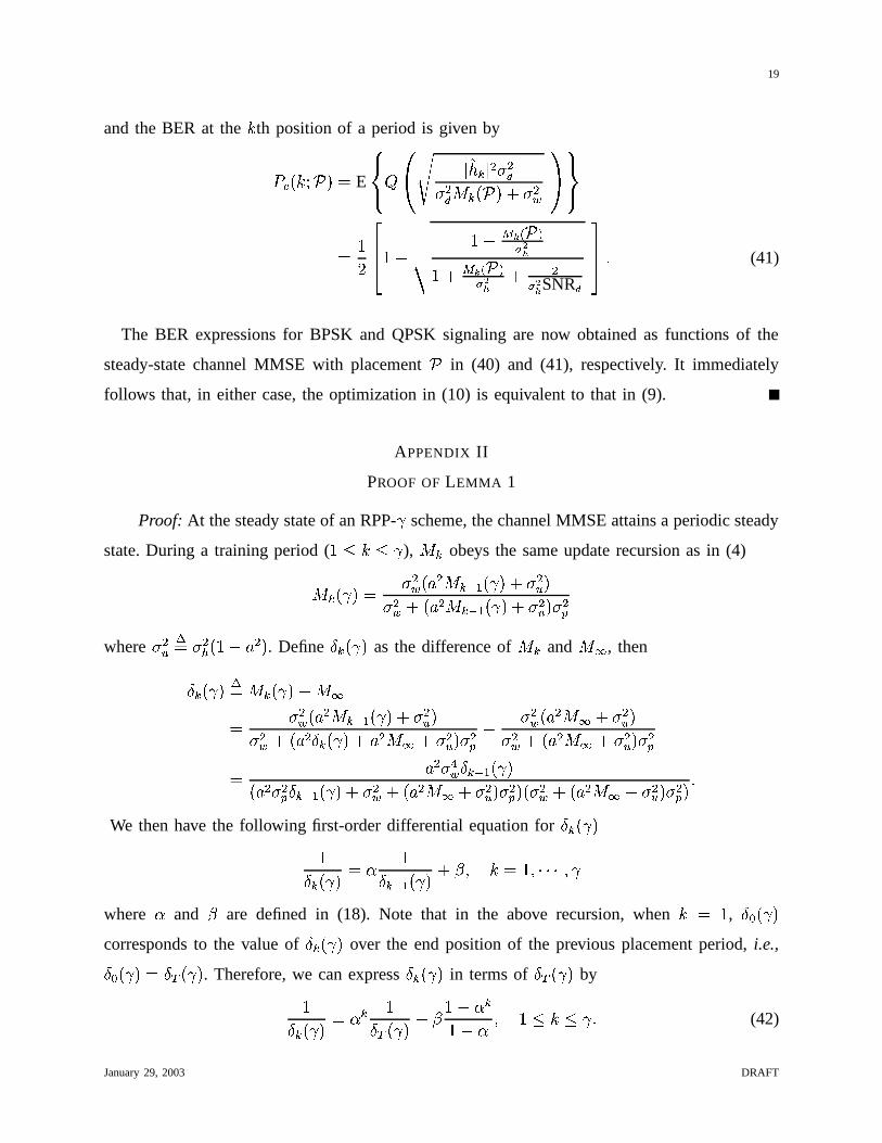
and the BER at the � th position of a period is given by

�� / � � E

�� / � " ��

��

��

�� % � �

� % � + � / �� + � / �� SNR �

�� (41)

The BER expressions for BPSK and QPSK signaling are now obtained as functions of the

steady-state channel MMSE with placement / in (40) and (41), respectively. It immediately

follows that, in either case, the optimization in (10) is equivalent to that in (9).

APPENDIX II

PROOF OF LEMMA 1

Proof: At the steady state of an RPP- � scheme, the channel MMSE attains a periodic steady

state. During a training period ( � � � � � ),

�� obeys the same update recursion as in (4)�

� � � � � �� " �� " �� B

where �� %"� � � . Define � � � � � as the difference of

�� and

�� , then� � � � � �� %

��

� ��

��

�� B % ��

�� " ��

� " �� B�

� � �� B � � � � � � � ��

� �� B � � ��

� " �� B ��

We then have the following first-order differential equation for ��

� ��

where�

and � are defined in (18). Note that in the above recursion, when � � � , �� corresponds to the value of �� over the end position of the previous placement period, i.e.,�� ! � � � . Therefore, we can express � � � � � in terms of � ! � � � by

�� ! � � � � ��% � �� % � � � � � � �

�(42)


20

During data transmission ( � � � � � - ), the updating recursion for

�� is in (7). Therefore,� � � � � � � � � � � � � � � � � � � � %"� � � � � � � � � � � � � � � �� -

�(43)

From (42-43), � � � � � and � ! � � � satisfy the following relations�� # � � � � �� ! � � � ��

� %"� � � �� (44)

where for a given � , we have used the relation - � � � � . The steady-state equation for � ! � � � is

then given by�� ! #"�$&% '�)('* �,+.-0//� 132 � ��4 '�5��0�6�� 7 � 8� * � 2 +.-0// ".9,:<; �=�> � ��! #" � � '� * � 2 +.-0// "�9?:@; �=BADC (45)

Solving the above equation, we have the expression of � ! � � � , as a function of � , given in (15).

From (7), for any RPP- � scheme, the expression of the steady-state channel MMSE

��

over each data symbol is then obtained in (13) and (14).

APPENDIX III

PROOF OF THEOREM 1

A. The Algebraic Proof

Proof: We begin with the following lemma.

Lemma 2: For� �� and

�FE � E � E � , and G 'IH , J � G � � � � �LK� �NM K is a monotone decreasing

function.

Proof: We need to show that for any given GPO �

��% �#Q # ��% � Q # � E � % �6Q

� % � Q R ��S"� � � %"�6Q # �� %"� Q E � % ��Q # �

� % � Q � (46)

Let ��.T � � � ��U KWV �� U K . Then, to show (46) is equivalent to show that �

�.T � is monotone increasing

for�XEYTZE � . Differentiate �

��T � w.r.t.T

, we obtain

� �� T � % � G � � T Q � � % T Q � G T Q � � � � % T Q # � �� % T Q � �

�T Q � � � � % T � � G % T � � T T � �� T Q � � � �� % T Q � �[ �


21

where the inequality is due to� E TZE � , and thus,

T � � T T � �� T Q � � � E G . Therefore,

the inequality (46) holds, and J � G � is monotone increasing.

Lemma 3: For� �� and

�XE �� E � , and G ' H , let J � G � � � � � K� �NM K . Then,�� J � G � E J � G � � E � J � G � � (47)

Proof: We need to show�� %"�6Q� % � Q E � %"�#Q # �

� % � Q # � E �� % �6Q� % � Q

i.e.,�� % � Q # �� % � Q E � %"� Q # �

� %"� Q E �� % � Q # �� % � Q

Let ��.T � � � ��U K4V �� U K . Then, to show (47) is equivalent to show

�� E � � � � E �� E �� E �

�(48)

Notice that, for�7E T E � , �

��T � [ � . From Lemma 2, we know � ��T � is monotone increasing.

Therefore, for any�XE �� E � ,

� E � � � � E � .1%� � � � � � � �� G � � E �� (49)

where we use the fact that GPO � . By the same argument, we have

� � � � E ��

(50)

Combine (49) and (50), we have (47).

Using Lemma 3, we then obtain a property of � � that is needed in the optimization in the

following lemma.

Lemma 4: For � � defined in (17), we have�� [ �

�� # � � (51)

Proof: Notice that � � ,�

and � are not functions of � . From (19) and (12),� � � � � � .

From (18), since�IE � E � , and SNRB [ �

, we have� [ � . And from (18), � [ �

. Thus� � � � % � � [ �. From (17), this implies that � � [ �

. Then, to show (51), it is equivalent to show� � % �� %"� � �� [ �

�� % �� V �

��%"� � �� # �2� �which immediately follows Lemma 3.


22

Proof of Theorem 1: Rewrite � ! � � � in (15) as� ! � � � � �M �� M ��

We will prove that � ! � � � monotonic increases with � , or equivalently,� ! � � � � �� ! � � � �� (52)

monotonic decreases with � . We fist show that � � � � � is monotone decreasing. Let� �� % � � � � .

From � � and � � in (17) and (16), we have� �� % � � �� %"� ��

� � � � ��

� � � �� % � �

� ��

�� % � �

�(53)

As we have shown in Lemma 4,� [ � , we have

� E � � �� E � �� E ��

By Lemma 2, it follows that J � � � � is monotone decreasing. Also, J � � � � is monotone decreasing.

Notice that � � ,�

, and � are not functions of � . Also,� [ � and � � [ �

. Therefore, � � � � � in

(53) is monotone decreasing.

Again, by Lemma 2, � � in (16) is a monotone function of � . Since � � [ �, from above, it

follows that � ! � � � [ �. Notice that for any � O � , � ! � � � is a positive root of the following

quadratic equation� � % � �� % ��

(54)

whereas the other root of is negative. Therefore, to show � ! � � � monotone decreases, i.e.,� ! � � � � E � ! � � � � � � O � (55)

it is enough to show � � � �� ! � � � % � � # �� # � � ! � � � % �� # � [ ��

(56)

Substitute (52) in (56), we have � � � ��

� �� % � � # �� # � � � �� % � � # �� # � � � �� % �� # � (57)

Since � � � � � monotonic decreases, we consider the following three cases:


23

1)� E M � V �� V � E M �� : In this case, � � � in (57) satisfies

� � � [ �� % � � �� % � �� % �� # �

��

�� % �� # � �[ �

The last inequality holds because the first two terms are both positive, and the third term is

also positive by Lemma 4.

2)M � V �� V � E@�XE M �� : Rewrite � � � in (57) as

� � � � ��

% � � # �� # � � � �� % � � # �� # � � � � ��

�� % �� # � �By the assumption of the sign and Lemma 4, each term is positive. Therefore, � � � [ �

.

3)M � V �� V � E M �� E �

: In this case, we have � � � [ �� ! � � � �� % �� # � (58)

�� ! � � � % �

� � � � �� % �� # �� ! � � � �

�

�� % �

�� # � �[ �(59)

where inequality (58) is because � � [ �, thus

% � � # �� # � � � �� [ � � # �� # � � � �� [ ��

and inequality (59) follows from Lemma 4.

Combining 1)-3), we have (56), and thus (55). Therefore, � ! � � � monotone increases with � .

Since � ! � � � �� ! � � � %

�� , and

�� is not a function of � , it follows that

� ! � � � also a

monotonic increases with � . Therefore, by (11), &� � � is a monotone increasing function of � ,

and it immediately follows that

� � � �"!$#&%/.10� &� � � � ��

Under this placement, � !�� in (44) can be obtained and we have $� � � �� in (21).


24

B. The Graphic-Aided Proof

Here we give a more intuitive graphic-aided proof using Fig. 4.

For a RPP- � scheme, during training, from (42), we have� � � � � � � ! � � �� ! � � � �

� � � �� + ��

�(60)

Thus, � � � � � exponentially decreases with rate� � � � � � . During a data block, it follows from (43)

that� � � � % � � � � � � exponentially decreases at rate � � � � � � � .

PSfrag replacements

�

�

��

�

� �

� � ��

� � �

� ��

� �

� �

� ��

� �

� �

� � + �� V � ��

(a)

(b)

Fig. 4: Proof of Theorem 1

figureFig. 4 (b) and (a) describe the placement pattern / and the corresponding steady-state trajec-

tory of � � � � � � �� %

�� , respectively. For fixed pilot percentage � consider two schemes,

RPP- � � with / � � � � � �:8 � � , and RPP- � � with / � � � � � �:8 � � , where �C� [ � � . Shown in the left

part of Fig. 4(b) is the RPP- � � scheme, where the placement period is - � . Indexes � and ��denote the end positions of the data blocks in the

� ' % � � th and ' th placement periods under

RPP- � � , respectively. Index � denotes the end position of the pilot cluster in the ' th period.

Assume that in the� ' % � � th and ' th placement periods, the channel MMSE is at its steady

state. The corresponding � � � � � � at � and �� is � ! � � � � � . The trajectory curve �� of � � � �C� �is shown in Fig. 4(a). Because the changing rates of �� during pilot and data cluster are

exponential, �� and � � � � � are both exponential. The trajectory curve �� in Fig. 4(a)

is equivalent to � � �� , assuming RPP- �C� . Now, after the ' th period, we change the placement

to RPP- � � , shown in the right part of Fig. 4(b), where indexes �!� and �� denote the new end

positions of pilot and data cluster in the period, respectively. The change of placement results in

the new MMSE. Denote � � � # �2�� ) ' - � � + %

�� , and similarly � � � # �2�! � � � � � over �� . Then,� � � # �2�� is still on the trajectory curve �� in Fig. 4(a). Because for fixed pilot percentage


25

� , � � � � � � 8 � � 8 � , we have � � � � � � � � � � � � � � � � � � � � , shown in Fig. 4(a). Because �� and

� � � � �� are exponential, from the geometry, we have� � � # �2�� ! � � � � � � � � ��

This implies that � � � # �2�! � � � � � � � ! � � � � � . Consequently, � � � �! � � � � � � � ! � � � � � , for � [ ' . At the steady

state of RPP- � � , � ! � � � � � � � .1%�� # �2�! � � � � � � � ! � � � � ��

Because $� � � � � � ! � � � �

�� and

�� is not a function of � , we have

$� � � � O &� � � � , for� � [ � � . The minimum

$� � � can be obtained using Lemma 1.

APPENDIX IV

PROOF OF THEOREM 2

Recall that � � is the index for the end position of the�th data block relative to the beginning

of a period. We have the following lemma.

Lemma 5: Given / � � 0 ��2 � , with . pilot clusters in a placement period, then for any � �� . , �

� � 0 ��2 � �� 10 ��2 %�� (61)�

� �� 0 ��2 � O � � � � 0 ��2 %�� (62)

where � � denotes a �� . unit row vector with 1 at the�th entry and 0 elsewhere.

Proof: We use Fig. 5 to assist our proof. The figure describes the placement pattern / in

��

PSfrag replacements

��

Fig. 5: Proof of Lemma 1

figure

a period, and the steady state trajectory of �� / � � � � � � / � % � � � . Relative to the beginning

of a period, let � and � denote the end positions of the� � %�� th and

�th data block, and


26

� the end position of the�th pilot cluster. Let / � � � 0 ��2 � � be the new placement satisfying

2 � ��2 �� %�� . Then, showing (61) is equivalent to showing� � � 0 �2 � � E � � � 0 ��2 � �For simplicity, we denote � �� as � � � 0 ��2 � � and � � as � � �10 ��2 � , and similarly those of other points.

Assume in the� ' % � � th placement period, the MMSE is at its steady state. In the ' th period,

we move the�th pilot cluster right by one step. Let � � � � � and � � � � �� . This results

in the new MMSE at� ' % � � - �� and thereafter. Denote � � � � �� ) � ' % � � - �� + %

�� , and

similarly � � � � �� and � � � � �� . Then, from (42) and (43), we have�� % � � � � � � �� (63)

The one-step increment on the trajectory � � � is � � � � � % � � � � � � � % � � � . If we can show� � � � �� E � � � � � (64)

then � � � � �� E � � . Consequently, � � � � �� E � � ,� � [ ' and � �� .1% �� E � � . Therefore, we

only need to show (64). Let � � � � �� , where �� [ �. From the first equation of (63), we

have � � � � � %"� � � � � � � % � � � . From the second and third equations of (63), we have� � � � �� % � � � � � ��

� � ��) � � �� + )� � �� + % ��

� �� % �� % � �� %"� � �

� � � � � � % � � �) � � �� + )� � �� + % � � � % � �� E � � %"� � �

�� % � � � % � � � % � �� E �

where the inequalities are due to� [ � . Therefore, we have proved (61). By a similar argument,

we can show (62).

Lemma 6: Given � , for any0 �=) � �� 65 + , � 2 � '�� 5��

, such that�� 10 ��2 � � �

�� 0 ��2 � � � %'. 02 $� 0 ��2 �

�(65)


27

Proof: Let 2 � �#) 8 � �� :8 � + , � � � � . . For fixed 8 � # � � �� :875 , let

� � � �10 ��2 � �� %'�)(�� 0 �2 � � 2 �� "! # %'. 0� � � � �10 ��2 � �

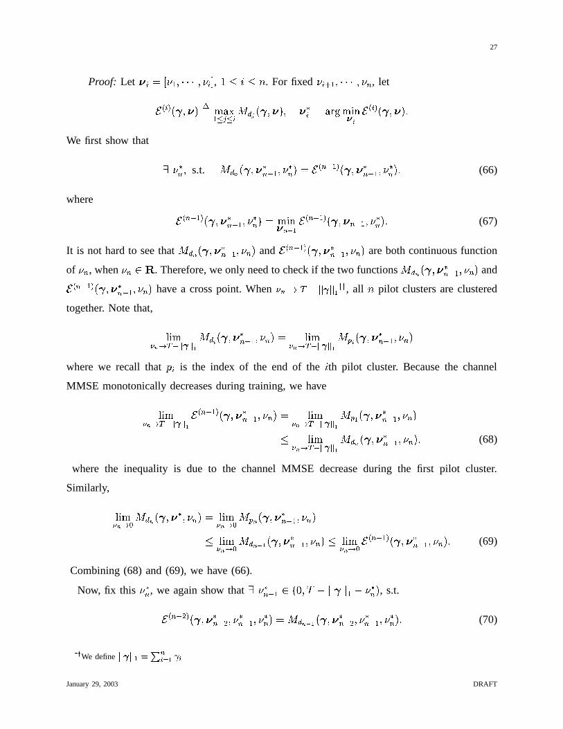
We first show that

� 8 �5 � s.t.

�� 0 �2 �5 � � ��8 �5 � � � 5 � �2� � 0 �2 �5 � � ��8 �5 � � (66)

where � 5 � �2� � 0 �2 �5 � � ��8 �5 � � %'. 02 � �� 5 � �2� � 0 ��2 5;� ��:8 �5 � � (67)

It is not hard to see that

�� 0 �2 �5 � � ��875 � and

� 5;� �2� � 0 ��2 �5;� � �:875 � are both continuous function

of 875 , when 875 ' � . Therefore, we only need to check if the two functions

�� 10 �2 �5 � � ��875 � and

� 5;� �2� �10 ��2��5 � � �:875 � have a cross point. When �� , all . pilot clusters are clustered

together. Note that,

� .1%� � � ! �� 0 �2 �5 � � ��875 � � � .1%� � � ! �� B �10 ��2 �5 � � �:875 �where we recall that - � is the index of the end of the

�th pilot cluster. Because the channel

MMSE monotonically decreases during training, we have

�1. %� � � ! �� 5;� �2� �10 ��2 �5;� � �:875 � � � .1%� � � ! �� B � � 0 ��2 �5;� � �:8�5 �� .1%� � � ! �� 0 ��2 �5 � � �:8�5 � � (68)

where the inequality is due to the channel MMSE decrease during the first pilot cluster.

Similarly,

�1. %� � � �

�� 10 ��2 � �:8�5 � � � .1%� � � �

�B � � 0 ��2 �5 � � �:8�5 �� .1%� � � �

�� 0 �2 �5 � � ��875 � � �1. %� � � �

� 5 � �2� � 0 ��2 �5 � � �:8�5 � � (69)

Combining (68) and (69), we have (66).

Now, fix this 8 �5 , we again show that� 8 �5;� � ' �� - % �1� 0 �1� � %"8 �5 � , s.t.

� 5 � � � � 0 ��2 �5 � � �:8 �5 � � ��8 �5 � �� 0 ��2 �5;� � �:8 �5 � � �:8 �5 � � (70)

*�*We define

�� A�� January 29, 2003 DRAFT

28

Again, it suffices to check if the two functions have a cross point by checking the two end point

values that 875;� � can take. Similar to (69) above, we have

�1. %� � � � �

�� 0 ��2 �5;� � �:8�5 � ��:8 �5 � � �1.1%� � � � �

� 5 � � � � 0 ��2 �5 � � �:8�5 � ��8 �5 ��

Assume there is no cross point, i.e.,

�� 0 �2 �5 � � ��875 � � �:8 �5 � E � 5 � � � �10 ��2 �5 � � ��875 � � �:8 �5 � , for

875;� � ' �� - % �1� 0 �1� � % 8 �5 � . Then, � 5 � �2� � 0 ��2 �5 � � �:8 �5 � � %/.10 � � � � 5 � � � � 0 ��2 �5;� � �:8�5 � ��:8 �5 � . By

Lemma 5, it follows that

8 �5 � � � �"!$#&%/.10� � �� 5 � � � � 0 ��2 �5 � � �:8�5 � ��:8 �5 � � - % � � 0 �1� � %"8 �5i.e., when all first

� . % � � pilot clusters are together. Then, we have

� 5 � �2� � 0 ��2 �5 � � �:8 �5 � � �1. %� � � � ! �� 0 �2 �5 � � ��875 � � �:8 �5 � � � B � �10 ��2 �5 � � �:875;� ��:8 �5 �E � �� 0 �2 �5 � � ��8 �5 � �This contradicts our earlier conclusion in (66). Thus, we have (70). From (66)-(67),�

� � � �10 ��2 �5 � � ��8 �5 � � �:8 �5 � � � 5;� � � �10 ��2 �5;� � �:8 �5;� � �:8 �5 �O � 5;� �2� � 0 ��2 �5;� � �:8 �5 � � � � � � 0 ��2 �5 � � �:8 �5 ��

(71)

Recursively, for fixed 8 �� # � �� :8 �5 , we can show that� 8 �� ' �� - % �1� 0 �1� � % < 5� >�� # � 8 �� s.t.

for � � � � . ,

�� 10 ��2 �� :8 �� 8 �5 � � � � � �2� � 0 ��2 �� :8 �� :8 �5 � .

Let 2 � �=)98 �� :8 �5 + , where 8 �� is obtained as above. Then similar to (71), we have

�� 0 �2�� O�

� V � �10 ��2 � � , for � � � � . % � , and

�� 10 ��2 � � � � � �2� �10 ��2 � � � � � � � �10 ��2 � � . By Lemma 5,

it is easy to see that�� 0 ��2 � � � %'. 02 � � � � � 0 ��2 � ��8 �� 8 �5 � � � � � � 0 ��2 � � � � �� 0 ��2 � �

�Using the same argument recursively, we finally have

�� 10 ��2 � � �

�� 0 ��2 � � , for � � � � � � � . .

By Lemma 5, it follows that under 2 � , $� � ��2 � � reaches the minimum, and we have (65).

Proof of Theorem 2: By Lemma 6, we have the optimal 2 ( ' � 5) for each choice of

0,

denoted as 8 �� . The optimization of the placement can be rewritten as

�10 � ��2 � � � �"! # %'. 0� $� 0 ��2 ��

(72)

Given � and - , we fixed the number of pilot clusters in a period . and show that the optimal

placement is the one that reduces to RPP- � , and eventually by Theorem 1, the result follows.


29

1) The Two-Cluster Case (n=2):

Lemma 7: Assume . � � . Then, the optimal placement is given by

/ � � � ) � � �C+ ��) 8��8 + � � (73)

Proof: We give a geographic proof. By Lemma 6, for a given0 � ) �� + , there exist

2 �� , such that�� 0 ��2 �� 0 ��2 �� %'. 02 $� 0 ��2 �

�(74)

Now we need to show that, for / � � � ) � � �C+ �7) 8 �:8 + � ,�� / � � � � � � � / � � � $� / � � � &�10 ��2 ��

�(75)

Fig. 6 shows the trajectory of � � � / � under / � � 0 � 2�

� � at the steady state for . � � case.

PSfrag replacements

�

�

��

�

�

� �

� ��

� �

� �

� ��

�

��

��

��

�

�

Fig. 6: Proof of Lemma 7

figure

The curve � � � � � � � is the trajectory for the fist pilot cluster and data block. The corresponding

positions for indexes are also shown in the placement for one period of transmission. Then,� � � / � is on the trajectory �� !� � � � . Note that � � and � on � � � � � � � correspond to the same

point in the placement. Let � � � �C� � � � � � and 8 � � 8 � 8 � � � � . At the steady state of / ,

suppose for the next ' th period, we change the placement to / � � � ) � � �C+ �7) 8 �:8 + � . We denote

� ( � � ) as the position of the end of the first pilot cluster under / � . Then, � � � �� / � � is still

on the trajectory �� . The position � ( � � ) on the trajectory curve satisfies � � � � �

and � � � � � � � � . Since � � � � / � � � � � / � and rate of change of � � � / � during training and data


30

transmission, respectively ((60) and (43)), by the geometry property, we have � � � �� / � � � � � � �� / � .This implies that � � � �� / � � � � � � � / � �� / �Thus, � � � �� / � � E � � � �� / � � , for � [ ' . At the steady state of / � ,� � � � / � � � �1. %� �� / � � � � � � / � �From (75), because

0is arbitrary, we have

&� / � � � %'. 0/ &� / ��

2) General n-Cluster Case: For a placement period with . pilot clusters, we use the equalizing

rule in Lemma 6 and apply the result in Lemma 7 to the placement of each two consecutive

pilot clusters.

Given any placement / � �10 ��2 � , we construct the following procedure. Denote� 0 ��2 � at the

�th step by

�10 � � � ��2 � � � � , then

(1) At step i, by Lemma 6, there exists 2 �� , such that, for� �� . ,

&�10 � � � �2 �� 0 � � � ��2 �� %/.102 � $� 0 � � � ��2 � � � � � (76)

Denote0 �

� � 0 � � 2 �� 2 �� .

(2) Let � � � . Using the result in Lemma 7, we equalize each two consecutive pilot cluster

lengths in order:

(i) Define the ’averaging’ matrix� � as

� � � � � � � �� ' � � �� )�� ' � � �� )��

otherwise

�We average the lengths of the � th and

� � � � th pilot clusters, and the same to the� th and

� � � � th data blocks, while keeping the lengths of the rest of the pilot and

data clusters unchanged:

0 � � �� 0 � � �� 2 � � �� 2 � � ��


31

Then, from Lemma 7, we know that

$� 0 � � �� 2 � � �� $� 0 � � �� 2 � � �� (ii) By Lemma 6, there exists 2 �� such that, for all

� �� . ,

&�10 � � �� 2 �� 0 � � �� 2 �� %/.102 $� 0 � � �� 2 � �Let 2

� � �� 2 �� . Then, we have

$� 0 � � �� 2 � � �� $� 0 � � �� 2 � � �� (iii) If �

E . % � , then let � % � � � , repeat (i)-(iii).

(iv) Let�10 � � # �2� ��2 � � # �2� � � � 0 � � �5 � � ��2 � � �5 � � � . Then,

$� 0 � � # �2� ��2 � � # �2� � � $� 0 � � � ��2 � � � � �(3) Let

� % � � � . Repeat (1)-(3).

Repeat the above procedure. As� � � , we have

$� �1. %� �� 0 � � � � � .1%

� � � 2 � � � � � $� 0 ��2 ��

If we can show that

� .1%� � � 0 � � � � 0 � �=) � � �� C+ � (77)

� .1%� �� 2 � � � � 2 � �=)98�� :86+ � (78)

then, because / � � 0 �2 � is arbitrary, it follows that

$� / � � � %'. 0/ $� / �

and we prove Theorem 2.

Now, we show (77) is true. For a given0 � � � , define � � as the maximum difference of lengths

between the pilot clusters at step�:

� � � %�� (��> � � � � > � �� 5 � 0 � � � ) � +�% 0 � � � ) � + � �The procedure we describe in part (2) tries to even the lengths of all pilot clusters. After part

(2) is finished, we have

%'. 0�� 65 � �� # �2� ) � + ) O %/.10�� 65 � �

� � � ) � + ) � %��)(�� 65 � �� # �2� ) � + ) � %'�)(�� 65 � �

� � � ) � + ) �


32

Thus, we have

� � O � � # � O ��

Because the sequence � � � ) monotonically decreases and is bounded from below, its limit exists.

We now bound the decrement of � � . Because there are . pilot clusters, at the�th step, there

exists at least two consecutive clusters, say � th and� � � � th clusters, so that� � � � � ) � + % �

� � � ) � �,+ � O �

. � ��

After� . % � � times of the pilot clusters averaging process in part (2), the decrement of the largest

pilot cluster length, or the increment of the smallest pilot cluster length, is lower bounded by

%'�)( � � %'�)(�� 65 �� ) � + % %��)(�� 65 �

� � # �2� ) � + � � � %/.10�� 65 �� # �2� ) � + % %/.10�� 65 �

� � � ) � + �� O �� 5 � � . � �

�Then, it follows that

� � # � ��% �

� 5 � � . ��

(79)

Recall that � E � . Thus, �1. % � �� . The same argument applies to 2 � � � . Thus, we have (77)

and (78).

REFERENCES

[1] J. K. Cavers, “An Analysis of Pilot Symbol Assisted Modulation for Rayleigh Fading Channels,” IEEE Trans. on Veh.

Tech., vol. 40, pp. 686–693, November 1991.

[2] J. H. Lodge and M. L. Moher, “Time Diversity for Mobile Satellite Channels Using Trellis Coded Modulations ,” in Proc.

IEEE Global Telecommun. Conf., (Tokyo), 1987.

[3] S. Sampei and T.Sunaga, “Rayleigh Fading Compensation Method for 16QAM in Digital Land Mobile Radio Channels ,”

in Proc. IEEE Veh. Technol. Conf., (San Francisco, CA), pp. 640–646, May 1989.

[4] J. M. Torrance and L. Hanzo, “Comparative study of pilot symbol assisted modem schemes,” in Proc. 6th Conf. Radio

Receivers and Associated Systems,, pp. 36–41, Sept. 1995.

[5] M. K. Tsatsanis and Z. Xu, “Pilot Symbol Assisted Modulation in Frequency Selective Fading Wireless Channels,” IEEE

Trans. Signal Processing, vol. 48, pp. 2353–2365, August 2000.

[6] M. Medard, I. Abou-Faycal, and U. Madhow, “Adaptive Coding with Pilot Signals ,” in 38th Allerton Conference, October

2000.

[7] S. Ohno and G. B. Giannakis, “Average-Rate Optimal PSAM Transmissions over Time-Selective Fading Channels,” IEEE

Trans. on Wireless Communications, vol. 1, pp. 712–720, October 2002.

[8] J. Gansman, M. Fitz, and J. Krogmeier, “Optimum and Suboptimum Frame synchronization for pilot-symbol-assisted

modulation,” IEEE Trans. Signal Processing, vol. 45, pp. 1327–1337, April 1997.


33

[9] R. Negi and J. Cioffi, “Pilot Tone Selection For Channel Estimation In A Mobile OFDM System,” IEEE Trans. on Consumer

Electronics, vol. 44, pp. 1122–1128, Aug. 1998.

[10] M. Dong and L. Tong, “Optimal Design and Placement of Pilot Symbols for Channel Estimation,” IEEE Trans. on Signal

Processing, vol. 50, pp. 3055–3069, December 2002.

[11] C. Budianu and L. Tong, “Channel Estimation for Space-Time Orthogonal Block Code,” IEEE Trans. on Signal Processing,

vol. 48, pp. 2515–2528, October 2002.

[12] S. Adireddy, L.Tong, and H.Viswanathan, “Optimal Placement of Training for Frequency Selective Block-Fading Channels,”

IEEE Trans. on Info. Theory, vol. 48, August 2002.

[13] S. Ohno and G. B. Giannakis, “Optimal Training and Redundant Precoding for Block Transmissions with Application to

Wireless OFDM,” IEEE Trans. on Communications, vol. 50, December 2002.

[14] F. Ling, “Optimal Reception, Performance Bound, and Cutoff Rate Analysis of References-Assisted Coherent CDMA

Communications with Applications,” IEEE Trans. Communications, vol. 47, pp. 1583–1592, Oct. 1999.

[15] M. Dong, S.Adireddy, and L. Tong, “Optimal Pilot Placement for Semi-Blind Channel Tracking of Packetized Transmission

over Time-Varying Channels,” to appear in IEICE Transactions on Communication, March 2003; Available at

http://acsp.ece.cornell.edu/pubJ.html

[16] M. Medard, “The Effect upon Channel Capacity in Wireless Communications of Perfect and Imperfect Knowledge of the

Channel,” IEEE Trans. Information Theory, vol. 46, pp. 933–946, May 2000.

[17] A. Gaston, W. Chriss, and E. Walker, “A multipath fading simulator for radio,” IEEE Trans. Veh. Technol., vol. 22,

pp. 241–244, 1973.

[18] R. Iltis, “Joint Estimation of PN Code Delay and Multipath Using the Extended Kalman Filter,” IEEE Trans. Commun.,

vol. 38, pp. 1677–1685, October 1990.

[19] M. Stojanovic, J. Proakis, and J. Catipovic, “Analysis of the Impact of Channel Estimation Errors on the Performance

of a Decision-Feedback Equalizer in Fading Multipath Channels,” IEEE Trans. Commun., vol. 43, pp. 877–886, February

1995.

[20] T. Kailath, A. Sayed, and B. Hassibi, Linear Estimation. Upper Saddle River, NJ 07458: Prentice Hall, 2000.

[21] J. Proakis, Digital Communications, Third edition. McGraw Hill, 1995.

[22] M. Dong, L. Tong and B.M. Sadler, “Optimal Pilot Placement for Time-Varying Channels,” ACSP TR-01-03-02, Jan. 2003.

Available at http://acsp.ece.cornell.edu/pubR.html


34

0.9 0.91 0.92 0.93 0.94 0.95 0.96 0.97 0.98 0.99 10

0.1

0.2

0.3

0.4

0.5

0.6

0.7

0.8

0.9

1

Fading correlation coefficient a

max

MM

SE

SNR=20dB,η=0.2, σh2 = 1

γ=1γ=2γ=4γ= 10γ=20

0.9 0.91 0.92 0.93 0.94 0.95 0.96 0.97 0.98 0.99 110

−3

10−2

10−1

100


max

BE

R

SNR=20dB,η=0.2

γ=1γ=2γ=4γ= 10γ=20

Fig. 7: (a) Maximum steady-state channel MMSE &� � � vs. � . (b)

Maximum steady-state BER vs. � . ( � �� , SNR=20 dB)figure

0 5 10 15 20 25 3010

−2

10−1

100

SNR(dB)

max

BE

R

a=0.985,η=0.2

γ=1γ=2γ=4γ= 10γ=20

Fig. 8: Maximum steady-state BER vs. SNR ( � � ��

, � � � �� ).

figure

0.9 0.91 0.92 0.93 0.94 0.95 0.96 0.97 0.98 0.99 10

0.1

0.2

0.3

0.4

0.5

0.6

0.7

0.8

0.9

1


max

MM

SE

SNR=20dB, η=0.1

TDM:RPP−1Superimposed

0.9 0.91 0.92 0.93 0.94 0.95 0.96 0.97 0.98 0.99 110

−2

10−1

100

correlation coefficient a

BE

R

SNR=20dB, η=0.1

TDM:RPP−1 (max BER)SuperimposedTDM:RPP−1 (avg BER)

Fig. 9: (a) Max. steady-state MMSE vs. � . (b) Max. steady-state BER vs.� . (SNR=20 dB, � � � �� )

figure


35

0.9 0.91 0.92 0.93 0.94 0.95 0.96 0.97 0.98 0.99 10.1

0.2

0.3

0.4

0.5

0.6

0.7

0.8

0.9


max

MM

SE

SNR=5dB, η=0.1

TDM:RPP−1Superimposed

0.9 0.91 0.92 0.93 0.94 0.95 0.96 0.97 0.98 0.99 110

−1

100

correlation coefficient a

BE

R

SNR=5dB, η=0.1

TDM:RPP−1 (max BER)SuperimposedTDM:RPP−1 (avg BER)

Fig. 10: (a) Max. steady-state MMSE vs. � . (b) Max. steady-state BER vs.� . (SNR=5 dB, � � � �� ))

figure

5 10 15 20 25 3010

−2

10−1

100

SNR

BE

R

a=0.99, η=0.1

Superimposed TDM:RPP−1 (max BER)TDM:RPP−1 (avg BER)

5 10 15 20 25 3010

−2

10−1

100

SNR

BE

R

a=0.95, η=0.1

Superimposed TDM:RPP−1 (max BER)TDM:RPP−1 (avg BER)

Fig. 11: (a) Max. steady-state BER vs. SNR. (a=0.99, � � � �� ) (b) Max.

steady-state BER vs. SNR. (a=0.95, � � � �� )figure

0.1 0.15 0.2 0.25 0.3 0.35 0.4 0.45 0.510

−2

10−1

100

Percentage of pilot symbols η

max

BE

R

SNR=20dB, a=0.9

Superimposed TDM:RPP−1(max)TDM:RPP−1(avg)

Fig. 12: BER vs. � for � � ��, SNR=20 dB.

figure


Documents

Optimal Pilot Placement for Time-Varying Channels fileoutperforms RPP-1 in the other regimes. This demonstrates the potential for using superimposed training This demonstrates the