WORKING PAPER SERIES

Optimal Monopoly Investment and Capacity Utilization

under Random Demand

David B. Nickerson

Stanley S. Reynolds

Working Paper 1990-003A

http://research.stlouisfed.org/wp/1990/90-003.pdf

FEDERAL RESERVE BANK OF ST. LOUISResearch Division

411 Locust Street

St. Louis, MO 63102

______________________________________________________________________________________

The views expressed are those of the individual authors and do not necessarily reflect official positions of

the Federal Reserve Bank of St. Louis, the Federal Reserve System, or the Board of Governors.

Federal Reserve Bank of St. Louis Working Papers are preliminary materials circulated to stimulate

discussion and critical comment. References in publications to Federal Reserve Bank of St. Louis Working

Papers (other than an acknowledgment that the writer has had access to unpublished material) should be

cleared with the author or authors.

Photo courtesy of The Gateway Arch, St. Louis, MO. www.gatewayarch.com

OPTIMAL MONOPOLY INVESTMENT AND CAPACITY

UTILIZATION UNDER RANDOM DEMAND

April 1990

Abstract

Unique value-maximizing programs of irreversible capacity investment and capacity utilization are

described and shown to exist under general conditions for monopolist exhibiting capital adjustment costs

and serving random consumer demand for a nondurable good over an infinite horizon. Stationary

properties of these programs are then fully characterized under the assumption of serially independent

demand disturbances. Optimal monopoly behavior in this case includes acquisition of a constant and

positive level of capacity, the maintenance of a positive expected value of excess capacity in each period,

and an asymmetrical response of price to unanticipated fluctuations in consumer demand. Under a

general form of Markovian demand, the effect of uncertainty on irreversible capacity investment is also

described in terms of the discounted flow of expected revenue accruing to the marginal unit of existing

capacity and the option value of deferring the acquisition of additional capital. The option value of

deferring such acquisition, created by the irreversibility of capacity investment, is characterized directly

in terms of the value function of the firm, and is then shown to be zero in a stationary equilibrium with

serially independent demand disturbances. The response of investment to increase demand uncertainty

depends, as a result, directly on the properties of the marginal revenue product of capital. A non-negative

response of optimal capacity to increased uncertainty in market demand is demonstrated for a general

class of aggregate consumerpreferences.

David B. Nickerson Stanley S. ReynoldsUniversity of British Columbia University of Arizona

and Visiting Scholar,Federal Reserve Bank of St. Louis

We would like to thank Lanny Aryan, David Backus, Mukesh Eswaran, RobertPindyck, Neil Ramon, PatReagan, Todd Sandier, Bill Schworm and seminar participants at the 1988 Meetings of the Society forEconomic Dynamics and Controi, the Federal Reserve Banks of New York and St. Louis, North CarolinaState University, the University of Waterloo and the University of British Columbia for their helpfulcomments, correspondence, and discussion regarding an earlier version of this paper. Partial researchsupport for David Nickerson was provided by UBC-HSS Research Grant 5-57899. The usual disclaimerapplies.

Abstract

Unique value-maximizing programs of irreversible capacity investment and capacity utiliza-tion are described and shown to exist under general conditions for a monopolist exhibiting capitaladjustment costs and serving random consumer demand for a nondurable good over an infinitehorizon. Stationary properties of these programs are then fully characterized under the assump-tion of serially independent demand disturbances. Optimal monopoly behavior in this case includesacquisition of a constant and positive level of capacity, the maintenance of a positive expected valueof excess capacity in each period, and an asymmetrical response of price to unanticipated fluctua-tions in consumer demand. Under a general form of Markovian demand, the effect of uncertaintyon irreversible capacity investment is also described in terms of the discounted flow of expectedrevenue accruing to the marginal unit of existing capacity and the option value of deferring theacquisition of additional capital. The option value of deferring such acquisition, created by theirreversibility of capacity investment, is characterized directly in terms of the value function of thefirm, and is then shown to be zero in a stationary equilibrium with serially independent demanddisturbances. The response of investment to increased demand uncertainty depends, as a result,directly on the properties of the marginal revenue product of capital. A non-negative response ofoptimal capacity to increased uncertainty in market demand is demonstrated for a general class ofaggregate consumer preferences.

I. Introduction

The existence of uncertainty in consumer demand can exert a crucial influence on the invest-

ment, production and pricing decisions of firms. When investment in capital is irreversible, such

uncertainty can expose firms to risk from the possibility of having insufficient productive capacity

on hand in periods of robust demand, while in periods of slack demand firms are exposed to risk

from the opportunity cost of committing to suboptimal levels of current capacity, instead of re-

maining flexible to postpone investment to more advantageous future states. This tension between

committing to current investment or maintaining the flexibility to invest at a more propitious date

in the future can also directly affect the current pricing and production decisions of those firms

which have extensive market power, requiring managers to assess the trade-off between respond-

ing to unanticipated demand fluctuations through price adjustment or through an adjustment of

current production schedules.

When capacity constraints in the production technology and the irreversible nature of capital

investment represent bounds on the ability of a firm to profitably exploit current and future random

fluctuations in consumer demand, the influence of uncertainty on the investment, production and

pricing decisions of the firm is represented in the firm’s two types of decisions about the value of

capacity: (i) investment decisions, which affect future capacity; and (ii) production and pricing

decisions, which reflect the optimal utilization of existing capacity. The purpose of this paper is

to integrate these two types of decisions into a single intertemporal model capable of generating

explicit implications of demand uncertainty and capacity irreversibility for the nonstrategic invest-

ment, production and pricing behavior of a representative firm. Specifically, we consider optimal

investment, production and pricing rules for a risk-neutral monopolist exhibiting capacity adjust-

ment costs and serving random consumer demand for a nondurable good over an infinite horizon.

A one period-lag in the acquisition of productive capital exposes the firm to risk from the alter-

native possibilities of inadequate capacity and insufficient demand while decisions regarding the

utilization of existing capacity are made after the resolution of current uncertainty. These features

lead to important implications for the roles of uncertainty and irreversibility in influencing the

intertemporal behavior of investment, prices and capacity utilization.

Five propositions about monopoly behavior are offered. First, unique value-maximizing rules

for capacity, investment, production and pricing are shown to exist under an extremely general

Markovian specification of demand uncertainty and several characteristics of these rules are ex-

amined. The influence of uncertainty and irreversibility on capital investment are, when gross

investment is positive, described in terms of both the discounted flow of expected revenue accruing

to the marginal unit of capacity as well as the value of deferring the acquisition of an additional unit

of capital, which will be non-negative as a result of the irreversible nature of capital investment.

The flow of expected marginal revenue, and the value of deferring acquisition of the marginal unit

of capital, are respectively characterized directly in terms of the value function describing the firm’s

optimal dynamic program. Optimal capacity is shown to equate the discounted flow of expected

marginal revenue to the total cost of acquiring the marginal unit of capital, which consists of both

a direct cost and an opportunity cost of exercising the firm’s option to defer acquisition of this unit

to a subsequent period.

Second, four stationary properties of these rules are then characterized under the assumption

that disturbances to consumer demand display serial independence. Optimal monopoly behavior

in this situation includes the maintenance of both a constant level of capacity over time and,

in contrast to the analogous competitive industry, a positive level of expected excess capacity

in each period. Optimal monopoly behavior also includes an asymmetrical response of price to

unanticipated demand fluctuations, with any downward adjustment of price in response to a weak

state of demand being circumscribed by the market power of the firm and its optimal maintenance

of a measure of excess capacity. Finally, the option value of deferring acquisition of the marginal

unit of capital is shown to be zero in a stationary equilibrium with serially independent demand,

and the response of optimal capacity to a mean-preserving spread in the distribution of disturbances

to market demand, which in this case will depend entirely on the convexity of the marginal revenue

product of capital, is shown to be non-negative for a broad class of aggregate consumer preferences.

The role of demand uncertainty in the nonstrategic investment, pricing and capacity utiliza-

tion decisions of firms has been a topic of considerable interest in recent years and has generated

numerous analyses of each of these separate decisions. Lucas and Prescott (1971) demonstrated

the existence of optimal investment programs for risk-neutral firms in a competitive industry with

endogenous price uncertainty and gave a limited characterization of a stationary competitive equi-

librium with serially independent demand disturbances. Hartman (1972), Nickell (1977), Pindyck

(1982), Abel ((1983), (1984)), and Albrecht and Hart (1983), among others, subsequently exam-

ined the response of capital investment by competitive firms to increased uncertainty in consumer

demand, with disparate results. Jones and Ostroy (1984) provided a general characterization of the

value of flexibility, with an application to capital investment, in a simple finite-horizon model of

sequential decision-making. Smith (1969), Zabel (1972) and Meyer (1975) examined the influence

2

of demand uncertainty on the maintenance of excess capacity by monopolists operating in either a

static market or under a finite planning horizon. Appelbaum and Lim (1982) studied the differen-

tial responses of industry production to increased demand uncertainty in static monopolistic and

competitive equilibria. Reagan (1982), Schutte (1984), Amihud and Mendelson (1983) and Zabel

(1986) considered the role of optimal inventory policies of monopolistic firms in influencing the

response of prices to unanticipated serially independent demand fluctuations in stationary equilib-

ria. Nickell ((1974), (1978)) examined the influence of irreversibility on the investment decisions of

firms respectively operating under certainty or under uncertainty about the timing of a single shift

in demand, while Pindyck (1988) most recently characterized the marginal investment decision and

the value of deferring irreversible capacity investment in terms of financial option theory, using the

specific case of consumer demand evolving according to geometric Brownian motion.’ Each of these

papers uses a distinct model to study the influence of demand uncertainty on one unique aspect

of firm behavior. Our paper integrates all of these aspects into a single intertemporal model of

the firm. This allows us to describe the effects of uncertainty and irreversibility on the value of

a marginal unit of capacity under relatively general assumptions about market demand and capi-

tal adjustment costs and, in particular, to illustrate the recursive influence of current investment

decisions on the utilization of capacity, as reflected through production and pricing decisions, in

subsequent periods.

The paper is organized as follows. The model of the firm is presented in section II. The

existence and uniqueness of market equilibrium and the nature of the unique optimal investment

rule for the monopolist under a general Markovian specification of consumer demand are examined

in section III. Section IV characterizes stationary properties of optimal monopoly investment,

pricing and capacity utilization rules for the case of serial independence. Conclusions appear in the

final section.

II. The Model

We consider a monopolist producing a quantity q(t) of a nondurable good in each period t by

means of the single input of capital, k(t)~2 Production occurs under constant returns to scale so

that k(t) denotes the level of full capacity, q(t)/k(t) denotes the current level of capacity utilization,

and the production function may be written as:

0 ~ q(t) ~ k(t). (1)

Costs of adjusting capacity are represented by a nonlinear relation between investment and

3

capital in successive periods,

k(t + 1) = k(t)h(x(t)/k(t)), (2)

where x(t) denotes gross investment and h(.) is bounded, continuously different able, increasing and

strictly concave.3 Investment in capital is assumed at least partially irreversiHe, so that x(t) 0

and 0 < h(0) ~ 1, and depreciation in capacity is indexed by the parameter 6, so that S = h’ (1)

exists for 0 < 6 < 1, allowing maintenance of the capacity level k(t) to occur at the rate of gross

investment Sk(t).

Market demand in each period is described by a conventional inverse demand function,

p(t) = D(q(t),u(t)), (3)

where p(t) is the current product price and u(t) is a random disturbance. Under all realizations of

u(t), the inverse demand function is assumed to be twice-continuously differentiable with D, <0,

D2 > 0, and D, < (—q(t)/2)D,,, non-negative, finite and bounded above S at a zero level of

sales. The random disturbance u(t) is assumed to be a real-valued Markov process over a compact

support [st, u}, with a continuously-differentiable transition probability function f (u(t), u(t + 1)) .~

Revenue from current sales is defined by (2) to be:

G(q(t),u(t)) = q(t)D(q(t),u(t)). (4)

The qualities of the inverse demand function in (3) imply that, for any realization of the random

disturbance u(t), the function G (.) is twice continuously-differentiable, strictly concave in q(t),

bounded uniformly for all q(t) > 0 and, conditional on the capacity constraint (1), defined over

the compact interval [0, k(t)]. Expected marginal revenue from the minimal level of optimal sales

is also assumed to exceed the marginal cost of maintaining a constant level of capacity, so that

EG1 ~ u(t)) > 8, where ~(u(t)) denotes, for any realization u(t), an unconstrained maximum

for revenue from current sales in (4) .~ Using (4), the stochastic value of the monopolist is defined

as:

>~~t(G(q(t)u(t))— x(t)), (5)

where fi = 1/(l + r) is the constant discount rate and r > 0 is the riskiess rate of interest.6

The timing of the monopolist’s sales and investment decisions create a dependence of revenue

on existing capacity, k(t), and the demand disturbance, u(t). At the beginning of each period, the

monopolist observes the current realization of the inverse demand schedule and selects a level of

production and sales, q(t), to maximize current revenue in (4) subject to the constraint imposed

4

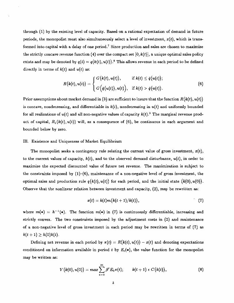
through (1) by the existing level of capacity. Based on a rational expectation of demand in future

periods, the monopolist must also simultaneously select a level of investment, x(t), which is trans-

formed into capital with a delay of one period.7 Since production and sales are chosen to maximize

the strictly concave revenue function (4) over the compact set [0, k(t)], a unique optimal sales policy

exists and may be denoted by q(t) = q(k(t), u(t)) ~8 This allows revenue in each period to be defined

directly in terms of k(t) and u(t) as:

( G(k(t), u(t)), if k(t) ~

R(k(t),u(t)) = (6)G (~(u(t)), u(t)), if k(t) >

Prior assumptions about market demand in (3) are sufficient to insure that the function R(k(t), u(t))

is concave, nondecreasing, and differentiable in k(t), nondecreasing in u(t) and uniformly bounded

for all realizations of u(t) and all non-negative values of capacity k(t) .° The marginal revenue prod-

uct of capital, R, (k(t), u(t)) will, as a consequence of (6), be continuous in each argument and

bounded below by zero.

III. Existence and Uniqueness of Market Equilibrium

The monopolist seeks a contingency rule relating the current value of gross investment, x(t),

to the current values of capacity, k(t), and to the observed demand disturbance, u(t), in order to

maximize the expected discounted value of future net revenue. The maximization is subject to

the constraints imposed by (1)—(6), maintenance of a non-negative level of gross investment, the

optimal sales and production rule q(k(t), u(t)) for each period, and the initial state (k(0), u(0)).

Observe that the nonlinear relation between investment and capacity, (2), may be rewritten as:

x(t) = k(t)m(k(t + 1)/k(t)), (7)

where rn(.) = h~’(.). The function m(.) in (7) is continuously differentiable, increasing and

strictly convex. The two constraints imposed by the adjustment costs in (2) and maintenance

of a non-negative level of gross investment in each period may be rewritten in terms of (7) as

k(t + 1) h(0)k(t).

Defining net revenue in each period by ir(t) = R(k(t), u(t)) — z(t) and denoting expectations

conditioned on information available in period I by E~(.),the value function for the monopolist

may be written as:

V(k(0),u(0)) = max>fltEox(t); k(t + 1) e C(k(t)), (8)

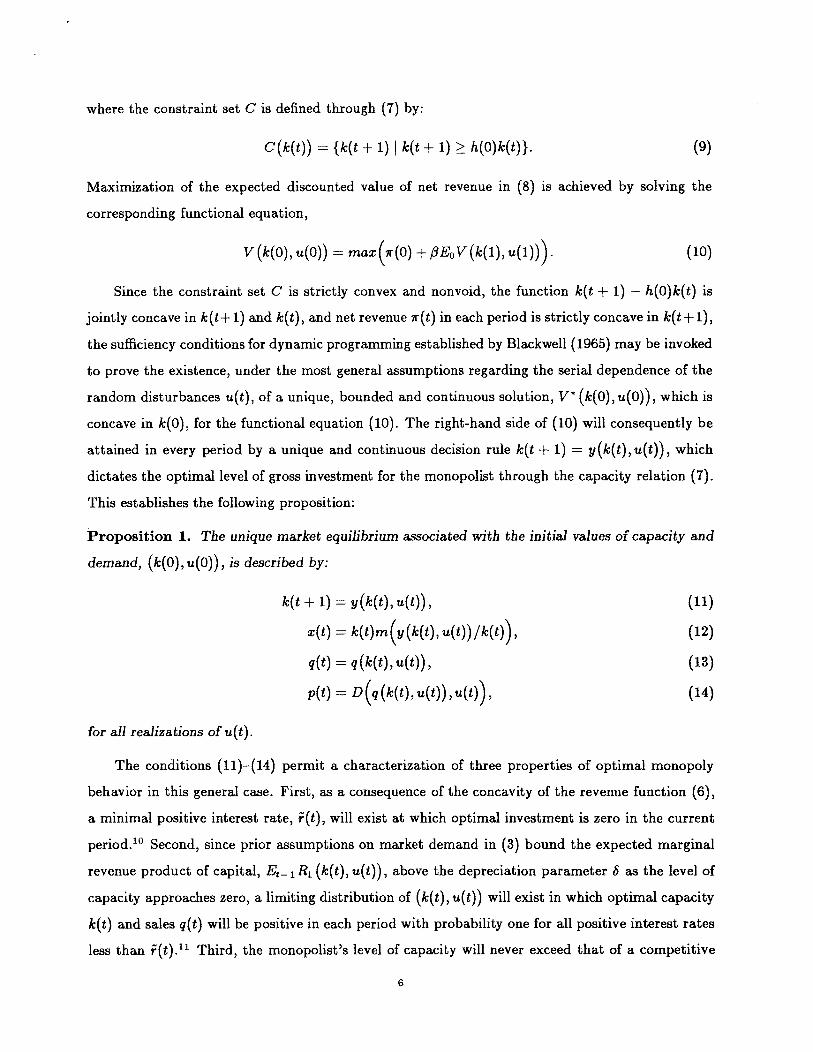
where the constraint set C is defined through (7) by:

c(k(t)) = {k(t + 1) k(t + 1) h(0)k(t)}. (9)

Maximization of the expected discounted value of net revenue in (8) is achieved by solving the

corresponding functional equation,

V (k(o), u(o)) = max(ir(O) + 13E0V (k(1), u(1))). (10)

Since the constraint set C is strictly convex and nonvoid, the function k(t + 1) — h(0)k(t) is

jointly concave in k(t+ 1) and k(t), and net revenue ir(t) in each period is strictly concave in k(t+ 1),

the sufficiency conditions for dynamic programming established by Blackwell (1965) may be invoked

to prove the existence, under the most general assumptions regarding the serial dependence of the

random disturbances u(t), of a unique, bounded and continuous solution, V~(k(o), u(0)), which is

concave in k(0), for the functional equation (10). The right-hand side of (10) will consequently be

attained in every period by a unique and continuous decision rule k(t + 1) = y(k(t), u(t)), which

dictates the optimal level of gross investment for the monopolist through the capacity relation (7).

This establishes the following proposition:

Proposition 1. The unique market equilibrium associated with the initial values of capacity and

demand, (k(0), u(0)), is described by:

k(t + 1) = y(k(t),u(t)), (11)

x(t) = k(t)m(y(k(t),u(t))/k(t)), (12)

q(t) = q(k(t),u(t)), (13)

p(t) = D(q(k(t),u(t)),u(t)), (14)

for all realizations of u(t).

The conditions (1 1)—(14) permit a characterization of three properties of optimal monopoly

behavior in this general case. First, as a consequence of the concavity of the revenue function (6),

a minimal positive interest rate, ~(t), will exist at which optimal investment is zero in the current

period.’0 Second, since prior assumptions on market demand in (3) bound the expected marginal

revenue product of capital, E~1R1 (k(t), u(t)), above the depreciation parameter S as the level of

capacity approaches zero, a limiting distribution of (k(t), u(t)) will exist in which optimal capacity

k(t) and sales q(t) will be positive in each period with probability one for all positive interest rates

less than ~(t).” Third, the monopolist’s level of capacity will never exceed that of a competitive

6

industry under similar conditions, precisely because the market power of the monopolist, reflected

in the concavity of the revenue function (6), implies that the expected marginal revenue product

of capital is always less than expected market price for any existing level of capacity.’2

A fourth property of monopoly behavior in this general case concerns the influence of irre-

versibility on the nature of the optimal investment decision. When investment is irreversible, the

timing of capital purchases assumes great importance in determining the value of the firm. De-

ferring the opportunity to acquire a unit of capital in the current period can be viewed as being

analogous to holding a financial call option written on the discounted flow of revenue expected to

accrue to this unit. Making the decision to acquire the unit of capital now is, as a consequence,

much like exercising such an option, and this exercise represents an opportunity cost to the firm

which must be evaluated, along with the direct acquistion cost, against the discounted expected

value of this unit, as implicitly measured by the value function V* (k(0), u(O)).

The optimal timing and magnitude of investment is reflected in the sequence of optimal capacity

levels, {k(s + 1)}~~,selected by the firm. Using the arguments of Benveniste and Scheinkman

(1979) regarding the differentiability of the value function (8), whenever the ratio of capacity in

successive periods exceeds h(0), for any initial stock of productive capacity k(t) extant in period

I, the optimal level of capacity selected in any period I for production in the subsequent period,

k(t + 1), must satisfy the first-order condition:

fiE~V,*(k(t + 1),u(t + 1)) = m’Qc(t + 1)/k(t)), (15)

where /9Ez V,~(k(t+1), u(t+i)) is the discounted expected value of the derivative of the value function

with respect to capacity. If x(t) is interpreted as the real cost of gross investment in the current

period, equation (15) indicates that optimal investment equates the direct real cost of acquiring the

marginal unit of capital, m’(.), to I3EtV,* (k(t + 1), u(t + 1)), the discounted expected value of that

marginal unit, evaluated along the unique optimal dynamic program of capital accumulation.’3

Now consider defining the functional S(k(t), u(t)) as

E~(~/3~’(R(k(t),u(t + j)) — k(t)m(1))), (16)

so that S(k(t),u(t)) ~ V*(k(t),u(t)). S(k(t),u(t)) is the value in any period t of the “constant

capacity” program of capital accumulation, a value which may not exceed, but may coincide with,

the value in that period of the optimal program of capital accumulation, V*(k(t), u(t)). By the

properties of the revenue function G(.), the functional S(.) is everywhere differentiable in its

7

arguments and

S, (k(t), u(t)) = ~ (k(t), u(t + j)) - 5)), (17)

where R1(k(t),u(t)) = max(0,G,(k(t),u(t))). S,(k(t),u(t)) is the expected discounted value of the

marginal unit of capacity, acquired in period t and evaluated in terms of the stream of future values

of the marginal revenue product of that unit, max(0, C, (k(t), u(t +j)), in each future period I +j.Equivalently, S, (.) is the expected value of the derivative of the value function associated with the

“constant capacity” program, S(.).

The difference between the values of the optimal and the constant capacity programs defines

the functional —J(k(t), u(t)),

—J(k(t), u(t)) = V*(k(t),u(t)) — S(k(t), u(t)) ~ 0, (18)

and when gross investment is positive, _J(.) has a derivative,

—.1, (k(t), u(t)) = V1 (k(t), u(t)) — S, (k(t), u(t)). (19)

Along the optimal path, the firm has the ability or option to acquire capital at any current or future

date I + j. Since — J(.) is the difference between the value of the optimal dynamic program and the

constant capacity program, the residual — J(.) may be interpreted as the value of preserving the

total sum of options to acquire each possible additional unit of capital at each future date. When

gross investment is positive, the derivative —J,(k(t), u(t)) represents the change in the current

value of that total sum of options, due to the acquisition of the marginal unit of capital when

current capacity is k(t). Consequently, J,(k(t),u(t)) can be interpreted as the opportunity cost of

killing the option to defer the irreversible acquisition of the marginal unit of capital to a subsequent

period. This cost depends on the forms of the revenue and adjustment cost functions and also on

the properties of the transition equation describing the stochastic evolution of consumer demand,

f(u(t),u(t + 1)).’~

Using (17) and (19) in (15), the necessary condition for an interior optimum in any period t

may be expressed as:

fiE~S,(k(t+ 1),u(t + 1)) = m’(ic(t + 1)/k(t)) + /‘3E~J,(k(t+ 1),u(t + 1)). (20)

Although it occurs in a general Markovian context, this expression has an interpretation analogous

to the interpretation of optimal investment behavior in the case of geometric Brownian motion

8

studied by Pindyck (1988): if capital is to be acquired in the current period, optimal capacity

k(t + 1) is defined by an equality between the expected discounted stream of marginal revenue

accruing to the last unit of capital acquired, /3E~S,(k(t+ 1), u(t + 1)), and the sum of two costs,

which are the direct cost of acquisition, m’(k(t + 1)/k(t)), and the expected opportunity cost

of exercising the option to acquire the marginal unit of capital in the current period, so that it

becomes productive in period t+1, /3E~J1(k(t+ 1),u(t + 1)).’~

IV. Equilibrium with Serially Independent Demand Disturbances

Explicit characterization of optimal monopoly behavior requires further restrictions to be placed

upon the distribution of disturbances to consumer demand. A case of special interest, examined

also in related contexts by Lucas and Prescott (1971), Reagan (1982), Abel (1983), Amihud and

Mendelson (1983), Schutte (1984), Zabel (1986) and others, involves the examination of a stationary

market equilibrium when demand disturbances display serial independence.’6

While market equilibrium still satisfies equations (1 1)—(20), the assumption of serial indepen-

dence implies that the optimal investment in each period depends only on the current level of

capacity, k(t) ~17 The independence of investment from any realization of the demand disturbance

u(t) in equations (7) and (12), the first-order condition (15) for capacity, the role of unit depre-

ciation costs S as a lower bound on the expected marginal revenue product of capital at a zero

level of capacity, as well as the existence results of Proposition 1 all serve to establish the following

proposition:

Proposition 2. If the distribution of disturbances to consumer demand displays serial indepen-

dence, then for any initial state (k(0),u(0)), there exist unique, non-negative sequences {k(s +

1),x(s),q(s),p(s)} and a positive constant k* which, for k(s + 1) defined by (15) and for s =

0,1,2,..., satisfy:

k~s+1~~fk(s+1) jfk(s) <k*; 21

‘ ‘ — 1. k(s)h(0), otherwise,

x(s) = f k(s)m(k(s + 1)/k(s)), if k(s) k*; (22)1. 0, otherwise,

q(s) = min(~(u(s)),k(s)), (23)

p(s) = max(D(~(u(s)),u(s)), D(k(s), u(s))), (24)

where k* represents the strictly positive, constant optimal level of capacity defined in the unique

stationary equilibrium by:

ER1(k*,u(t)) =S+rm’(l), (25)

9

and where gross investment satisfies

x(t) = Sk*, (26)

for all interest rates 0 < r < i~.

If the initial value of capacity, k(0), is less than the stationary optimum k~,gross investment in each

period is selected to yield a sequence of capital stocks, {k(s +1)}~~,which equate the direct acqui-

sition cost of the marginal unit of capital purchased in period s, m’(ic(s + 1)/k(s)), to its expected

discounted value, I3EtV,(k(s + 1), u(s + 1)). If the initial value of capacity exceeds the stationary

optimum, gross investment remains zero and capacity erodes at the rate h(0) until convergence

to the stationary optimum occurs •18 When capacity adjustment costs in (2) are strictly convex,

convergence in either case may be oniy asymptotic. This contrasts with the case of a constant ac-

quisition cost for capital, in which, assuming the value function is bounded, convergence will occur

in one period if the initial value of capacity is less than its st~tionaryoptimum.’9 Production and

price in each period are, by (1) and (3), always at the respective minimum and maximum of their

unconstrained and constrained values. Once the stationary equilibrium is attained, expression (25)

requires the expected marginal revenue product of capital, ER1 (k*, u(t)), to equal the user cost of

capital, which is the sum of the depreciation parameter S and the interest cost term rm’(1).

The description of the constant value of capacity in (25) may be used to characterize the

influence of capacity on optimal monopoly production and pricing behavior. Since existing capacity

is utilized to maximize profits in each period, inspection of equations (23) and (24) reveals that

optimal sales, q~,and price, p~,in the stationary equilibrium satisfy:I (~(u),D(~(u),u)), for u(t) < u*;

(q* (k* , u(t)) ,p~(k~,u(t))) = (27)

L~(k*,D(k~,u)), for if ~

where the threshold value of the demand disturbance, u*, is uniquely defined in the interior of the

support of u(t) through (4) and (7) by the condition ~(u*) = k*. Optimal production and sales,

described in (27), can never exceed the existing level of capacity and excess capacity will appear

for low realizations of consumer demand, as defined by u(t) < if.

A primary concern of previous studies of monopoly pricing and inventory behavior by Reagan

(1982), Amnihud and Mendelson (1983), Schutte (1984) and Zabel (1986) is the asymmetry exhibited

by the response of product price to variations in the random disturbance to consumer demand. Our

model shows that such an asymmetrical price response can also occur in markets with nondurable

goods and depends only on the existence of an upper bound on feasible sales in the current period.

The following proposition is an immediate consequence of equation (27):

10

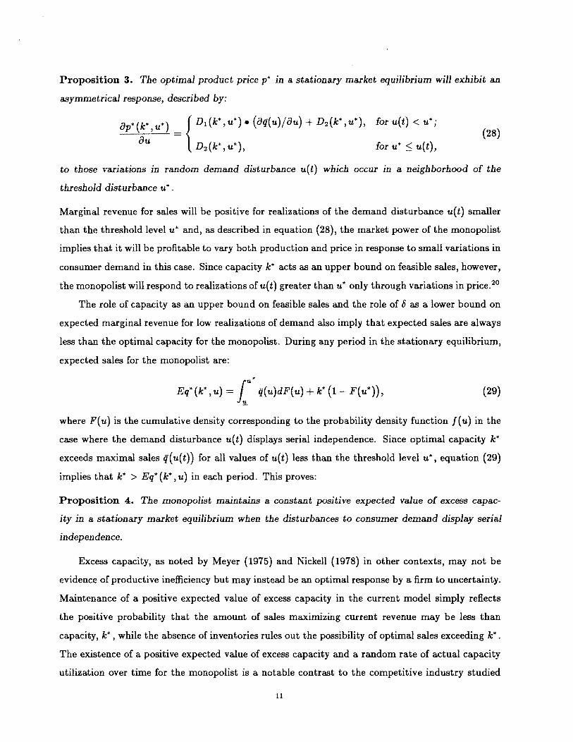
Proposition 3. The optimal product price p~in a stationary market equilibrium will exhibit an

asymmetrical response, described by:

* k4 if ~ Di(k*,u*). (thi(u)/c9u) +D2(k*,u*), foru(t) < u*;~(‘ )=~ (28)u ~D2(k*,u*), for if ~

to those variations in random demand disturbance u(t) which occur in a neighborhood of the

threshold disturbance if.

Marginal revenue for sales will be positive for realizations of the demand disturbance u(t) smaller

than the threshold level if and, as described in equation (28), the market power of the monopolist

implies that it will be profitable to vary both production and price in response to small variations in

consumer demand in this case. Since capacity k* acts as an upper bound on feasible sales, however,

the monopolist will respond to realizations of u(t) greater than if only through variations in price.20

The role of capacity as an upper bound on feasible sales and the role of S as a lower bound on

expected marginal revenue for low realizations of demand also imply that expected sales are always

less than the optimal capacity for the monopolist. During any period in the stationary equilibrium,

expected sales for the monopolist are:

Eq*(k*,u) = f ~(u)dF(u) + k* (1— F(u*)), (29)

where F(u) is the cumulative density corresponding to the probability density function 1(u) in the

case where the demand disturbance u(t) displays serial independence. Since optimal capacity k*

exceeds maximal sales ~(u(t)) for all values of u(t) less than the threshold level if, equation (29)

implies that k* > Eq* (k* , u) in each period. This proves:

Proposition 4. The monopolist maintains a constant positive expected value of excess capac-

ity in a stationary market equilibrium when the disturbances to consumer demand display serial

independence.

Excess capacity, as noted by Meyer (1975) and Nickell (1978) in other contexts, may not be

evidence of productive inefficiency but may instead be an optimal response by a firm to uncertainty.

Maintenance of a positive expected value of excess capacity in the current model simply reflects

the positive probability that the amount of sales maximizing current revenue may be less than

capacity, k*, while the absence of inventories rules out the possibility of optimal sales exceeding k*.

The existence of a positive expected value of excess capacity and a random rate of actual capacity

utilization over time for the monopolist is a notable contrast to the competitive industry studied

11

by Lucas and Prescott (1971), in which the absence of market power leads firms to produce at full

capacity in each period.

Previous studies by Hartman (1972), Nickell (1977), Abel (1983), Albrecht and Hart (1983)

and others have examined the response of the optimal capacity held by firms to increased uncer-

tainty in demand under a variety of alternative technologies, each involving production constraints

imposed by fixed factor stocks.2’ When efficient resale markets for capital exist, firms using such

technologies may respond to increased uncertainty, as represented by the conditional variance of

demand disturbances or by mean-preserving spreads in the distribution of such disturbances, by

maintaining or increasing their level of capacity, since the acquisition of excess capacity allows such

firms to hedge against the risk imposed by the possibility of unanticipated demand. When capital

investment is irreversible, however, and random fluctuations in demand occur in every period, firms

must assess the benefit of increasing capacity against the opportunity cost of exercising the option

to invest in a future and more favorable state of demand, as discussed by Jones and Ostroy (1984)

and Pindyck (1988).

Our model may be used to examine the effect of increased demand uncertainty on the optimal

stationary level of capacity held by a monopolist employing the production technology in (1) and

facing the convex costs of capacity adjustment embodied in (2). Uncertainty about future consumer

demand and a one-period lag in the acquisition of productive capital expose the monopolist to risk

from the alternative possibilities of suboptimal levels of excess capacity in situations of insufficient

demand and inadequate capacity in situations of excess demand. The acquisition of additional

capacity in response to increased uncertainty in demand could enhance the ability of the firm to

exploit unanticipated excess demand, as discussed by Jones and Ostroy (1984), but, as noted by

Pindyck (1988), when investment is irreversible, the ability to costlessly alter the rate of capacity

utilization allows the monopolist to only partially hedge against the transitory possibility of in-

sufficient demand, since the cost of exercising the option to acquire an additional unit of capacity

now will be nondecreasing, and may be strictly increasing, in response to the increase in demand

uncertainty.22

When the distribution of disturbances to consumer demand are serially independent, however,

the option value of deferring acquisition of the marginal unit of capacity is zero in a stationary

equilibrium. This may be seen directly from the general first-order condition (20). Recognizing that

f3E~S,(k(t+ 1), u(t + 1)) converges to the discounted value of the difference between the marginal

revenue product of capital and the marginal cost of depreciation, ((E~R,(k* , u) — S)/r) in this case,

12

the option value of deferring investment in the marginal unit of capacity may, using equation (20),

be written as

EtJ,(k*,u) =~~iEc(R,(k*,u)_ (5+rm’(l))). (30)

By equation (25), however, it may be seen that the right-hand side of (30) is zero after k* is

attained. The opportunity cost of exercising the option to acquire the marginal unit of capacity

is zero in a stationary equilibrium with serially independent disturbances to demand, because the

revelation of the state of demand in any period I contains no information about the evolution of

demand in any future period.23

Since the option value of acquiring the marginal unit of capacity is zero, the response of optimal

capacity to an increase in demand uncertainty is, by (25), entirely reflected in the convexity of the

expected marginal revenue product of capital. The market power displayed in the revenue functions

(4) and (6), may, however, preclude the convexity of the expected marginal revenue product of

capital in the current case. This would attenuate the attractiveness of additional capacity for the

monopolist, unless additional restrictions are placed on the aggregate representation of consumer

preferences in (3). By (6), the marginal revenue product of capital may be written as:

( C, (k(t), u(t)) > 0, for k(t) <

R, (k(t), u(t)) = (31)L~0, for k(t) ~(u(t)),

for any realization of the disturbance u(t). Inspection of (31) and (25), which defines the station-

ary value of capacity, k*, reveals that a sufficient condition for optimal monopoly capacity to be

nondecreasing in a mean-preserving spread of the distribution of the demand disturbance u(t) is

for the marginal revenue function, G,(k* , .), to be convex in the demand disturbance u(t) over the

support of the distribution of u(t).25

Since the convexity or concavity of the expected marginal revenue product of capital depends

directly upon the analogous property of the marginal revenue function C1 (k* , u(t)), further restric-

tions must be imposed on consumer preferences, as exhibited in the inverse demand function (3),

in order to assess the response of optimal monopoly capacity to increased demand uncertainty.26

The following proposition offers a sufficient set of such restrictions:

Proposition 5. The optimal stationary value of monopoly capacity, k*, will be nondecreasing in

a mean-preserving spread of the distribution of disturbances to consumer demand if the inverse

demand function (3) is convex in the demand disturbance u(t) and displays either additive or

multiplicative separability.

Proof of the proposition is straightforward and is left to the reader.

13

The creation of additional capacity as a response to greater uncertainty in consumer demand

may be described for the case in which the inverse demand function (3) exhibits convexity in u(t)

and multiplicative separability.27 Equation (31) indicates that increased uncertainty, as measured

by a mean-preserving spread in the distribution of u(t), increases the probability of states of high

demand, in which C, (k* , u(t)) and R, (k* , u(t)) attain larger values. The ability of the monopolist

to produce at less than full capacity simultaneously implies that R, (k* , u(t)) is zero in states of

low demand, which essentially truncates the lower tail of the distribution of demand disturbances.

Convexity of the marginal revenue product of capital in states of high demand implies that this

asymmetrical response of R1 (k* , u(t)) to the mean-preserving spread in u(t) acts to increase the

expected marginal revenue product of capital in (31). This increase in the expected marginal

revenue product of capital reflects the market power of the monopolist and creates an incentive for

the monopolist to expand capacity.

V. Concluding Remarks

Uncertainty in consumer demand and irreversibility in capital investment impose a tradeoff

between the relative advantages of enhancing productive capacity through committing to current

investment or maintaining the flexibility to invest in potentially more favorable future states. This

tradeoff, in turn, induces an important interdependence in the intertemporal production, pricing

and investment decisions of the firm. Specifically, when capacity constraints in production and the

irreversible nature of capital investment limit the ability of the firm to profitably exploit current

and future random fluctuations in consumer demand, the value of the firm is determined by two

types of decisions about capacity: investment decisions, which affect future capacity, and produc-

tion and pricing decisions, which reflect the utilization of existing capacity. The optimal timing of

investment, determined by the tradeoff between the relative advantages of a commitment to acquire

capital now versus the retention of flexibility to acquire capital later, influences, through the evo-

lution of capacity, the response of price and production by the firm to unanticipated fluctuations

in demand. Our analysis illustrates these essential points by integrating the two types of decisions

about capacity in a simple model of a risk-neutral monopolist serving random consumer demand

for a nondurable good over an infinite horizon.

Unique value-maxin-iizing rules for irreversible capacity investment and the utilization of capac-

ity are first shown to exist for the firm and are described under a general Markovian specification

of demand uncertainty. The optimal timing of investment is reflected by a value of capacity which,

in each period in which gross investment is positive, equates the discounted flow of revenue ex-

‘4

pected to accrue to the marginal unit of capacity acquired now to the total cost of that unit. This

total cost includes its direct acquisition cost and also the opportunity cost incurred by the firm in

exercising its option to acquire the marginal unit now instead of retaining flexibility by deferring

its acquisition to a later period. The stationary properties of these rules are then examined when

disturbances to consumer demand display serial independence.

Optimal monopoly behavior in a stationary equilibrium with serially independent disturbances

to consumer demand is described by four propositions. First, the monopolist acquires that constant

and positive level of capacity which equates the expected marginal revenue product of capital to

the constant acquisition cost of capital. Second, the response of product price variations in the

disturbance to consumer demand displays an asymmetry due to the role of existing capacity as

an upper bound on sales in each period. Third, this role of existing capacity also insures that

the monopolist will maintain a constant positive expected value of excess capacity in each period.

Finally, since the option value of deferring acquistion of the marginal unit of capital is zero in a

stationary equilibrium with serial independence, increases in demand uncertainty elicit a change

in the optimal level of capacity which ultimately depends directly on the influence of consumer

preferences on the expected marginal revenue product of capital. A sufficient condition for a non-

negative response of capacity to a mean-preserving spread in the distribution of disturbances to

consumer demand is for the inverse market demand function to display convexity in the demand

disturbance and additive or multiplicative separability in its arguments.

While expositional clarity is an important virtue of the model employed here, potential refine-

ments of our analysis, as a consequence, are numerous and include the consideration of more general

production technologies, endogenous delivery lags, the backlogging of unanticipated excess demand

and the influence of imperfect capital markets on the optimal investment profile. Such refinements,

which may be desirable for their realism, would leave intact the essence of many of our results while

complicating our analysis in obvious ways. The primary point we wish to emphasize in this paper

is that demand uncertainty and irreversible capital imply significant economic consequences for the

intertemporal behavior of the firm. Our model provides several interesting examples of these.

15

FOO TNO TES

1. Studies of irreversibility in the alternative context of a single discrete investment project, the

potential returns to which evolve according to diffusion processes, include MacDonald and

Siegel ((1985), (1986)), Jones and Heaney (1988), and others.

2. The results of our analysis would remain unchanged by the presence of additional productive

factorswhose quantities may be selected after the revelation of the current state of demand. The

essential nature of our results are also independent of the specific fixed-proportions production

technology and adjustment cost specifications in (1) and (2), which are adopted for tractability

and to facilitate comparison with the properties of equilibrium investment in the competitive

industry studied by Lucas and Prescott (1971).

3. The interpretation of capacity adjustment costs in terms of the strict concavity of the function

h(.) relies either on a direct nonlinear relation between physical investment and plant capacity

or on a strictly convex relation between investment costs per unit of capacity and the volume

of physical investment per unit of capacity, which could, for example, occur if the firm has

monopsony power in the market for physical capital or if the firm bears an increasing cost of

financing investment due to imperfections in capital markets. The usage of adjustment costs to

bound the value function V (.) appears, in the context of our model, to be both more realistic

and more tractable than the alternative assumption of exogenous delivery lags appearing in

Nickell (1978) and elsewhere. Although precise specifications may differ, this paper shares a

common assumption of such adjustment costs with Lucas and Prescott (1971), Hartman (1972),

Prescott (1973), Pindyck (1983), Abel (1983), Schutte (1984), Zabel (1986) and others.

4. These assumptions about the inverse demand function are sufficient, but obviously not nec-

essary, to generate those properties of the revenue functions in (4) and (6) required for an

optimum, and may be relaxed where appropriate. Similarly, all our results would be robust

under a relaxation of the assumption that the support of the transition probability function is

bounded, which is adopted only to allow increases in uncertainty to be represented by mean-

preserving spreads, rather than by conditional variance as in Abel (1983) and elsewhere.

5. The assumption that expected marginal revenue from the minimal level of optimal sales, ~

exceeds the marginal cost of maintaining a constant capacity level, EC,(~t),u(t)) 5, is

essentially a condition that there is a non-negligible amount of randomness in demand, and

may be alternatively but more labouriously expressed in terms of restrictions on the transition

16

function f(u(t),u(t + 1)). If, for example, the inverse demand function (3) is linear and the

distribution of u(t) is uniform over [~t’u], this condition is equivalent to assuming a sufficiently

large support for the distribution: ü — ~> 25.

6. Risk-neutrality is assumed on the part of the monopolist, since, as discussed by Nickell (1977),

it enables the pure effect of uncertainty, through its effect on expected returns to additional

capacity, to be separated from those ancilliary effects created by the increasing riskiness of

those returns. Risk-neutrality may also be justified by assuming the sufficiency conditions of

Malinvaud (1972) regarding spanning are satisfied. The effects of diversifiable and undiversifi-

able risk can easily be taken into account without changing our results, however, by replacing

the riskless rate with the rate of return on a portfolio of assets which is perfectly correlated

with the returns to the capital of the firm, as in Pindyck (1988). Burmeister and McElroy

(1988) present recent empirical evidence on the existence and nature of such a rate.

7. This formulation is intended, as in Lucas and Prescott (1971), Hartman (1972), Reagan (1982),

Pindyck (1983), Abel (1983) and elsewhere, to reflect the observation that pricing and produc-

tion decisions can be adjusted fairly quickly in response to variations in demand, subject to the

constraint imposed by current capacity, while changes in the level of capacity itself are costly

and occur only with a delay.

8. Lim (1982) examines the optimality of quantity-setting versus price-setting behavior with re-

spect to the convexity of the inverse demand function (3) in the random disturbance u(t).

9. Proof of this and other technical assertions below are available from the authors upon request.

10. Concavity of the revenue function (6) implies that the expected marginal revenue product of

capital will be non-increasing in the value of existing capital and that the optimal capital

stock is ultimately decreasing in the value of the interest rate r. Since optimality will require

that the expected marginal revenue product of capital equal the user cost of capital whenever

gross investment is positive, a time-dependent upper bound, ~(t), will exist on those values

of the parameter r compatible with positive investment. See Brock and Burmeister (1974)

and Burmeister (1981) for an extended discussion of this assumption and its analogous role in

assuring the existence of an interior stationary optimum in deterministic models of investment.

11. A constructive proof, based on analogues to lemmas 9 and 10 in Lucas and Prescott (1971),

can serve to establish the existence in the current model of a unique ergodic set, (/ç, /c) x [st’ u],in which 0 < /ç < k <oo. Since the marginal revenue product of capital approaches the value

17

of D(0,u(t)) for any realization of u(t) as the capital stock approaches zero, the assumption

D(0, u(t)) > 5 is then sufficient to establish that the ergodic set (jc, k) x [ii’ ü} is nonvoid. This

insures that optimal capacity will be positive in each period for all positive interest rates less

than ~(t).

12. See Lucas and Prescott (1971) and Appelbaum and Lim (1982) for a discussion of the respec-

tive intertemporal and static optimality conditions for a competitive industry under related

conditions. Prescott (1973) discusses the analogous nature of a perfect foresight equilibrium in

a deterministic version of the Lucas-Prescott (1971) model with an oligopolistic industry.

13. The first-order condition (15) may alternatively be expressed as

13E~R,(k(t+ 1),u(t + 1)) — /3[m(k(t + 2)/k(t + 1))

- m’((k(t + 2)/k(t + 1)) • ((k(t + 2)/k(t + 1))]

=rW((k(t+1)/k(t)).

If x(t) is the real cost of gross investment, optimal investment is seen to require the sum of

the expected discounted value of marginal revenue from capital plus the disounted saving in

investment costs from next period, obtained from an additional unit of capital in the current

period, to equal m’(k(t + 1)/k(t)), the marginal current investment cost from acquiring an

additional unit of productive capital for next period.

14. Since the functional J(k(t), u(t)) is interpretable as the total sum of options to acquire new units

of capital in the future, each of which is may be considered an asset with a stochastic return

corresponding to its marginal revenue product in each future period, the reduction of that

future stock of capital through the acquisition of a unit in the current period should, assuming

the usual stochastic domninance conditions are stisfied, result in a decline in the value of the

total sum of options remaining, so that —J, (k(t), u(t)) <0. Our model is, however, sufficiently

general to accomodate any sign for this derivative, where it exists.

15. Apart from its usage of discrete, rather than continuous, time, equation (20) encompasses the

condition for optimal irreversible investment in Pindyck (1988) and extends its interpretation

to the more general class of Markovian environments described here. The optimality condition

in Pindyck (1988), which applies to a model in which demand evolves according to geometric

Brownian motion, is derived by the direct usage of the financial option pricing technique in

Merton (1977), rather than by our more general method of stochastic dynamic programming.

18

16. The principal concessions exacted by the assumption of serial independence in the distribution

of demand disturbances are the optimality of a constant level of capacity over time and the

absence of serial correlation in prices, sales, and the rate of capacity utilization. The implica-

tions for monopoly behavior established under this assumption, however, will remain valid for

the antipodal case of serial dependence when they are interpreted as being conditional on the

state of demand realized in the previous period.

17. The assumption of serial independence also allows usage of the unconditional expectations

operator, E(.), and deletion of the explicit dating of future demand disturbances, u(t+s),s> 0,

in the propositions below.

18. Existence and monotonic convergence to a stationary equilibrium under serial independence is,

as a consequence, precluded only in the case where both S = 0 and k(0) > k*.

19. If adjustment costs were linear, as for example in Pindyck (1988), so that the direct cost of

acquiring a marginal unit of capital were a positive constant c, and if the value function were

to remain bounded in this case, which, for example, could occur if the conditionally expected

rate of growth in the demand disturbance u(t) were less than the riskless rate of interest, than

the optimal stationary value for capacity would be defined by the analogue to (15),

c = I3E0R,(k*,u(1)) + ,9ch(0),

and k, = k* for any initial value of capacity k(0) < k*. Strictly convex adjustment costs rule

out the necessity of one-period convergence. A variational argument may be used to derive a

sufficient condition for next-period convergence to k*, for any k(0) <k*, which is that

mr(k*/k(0) (k(1)/k(0)) • m”(kt/k(0)),

for any ~(1) satisfying k(0) <~(1)<k*.

20. Inspection of equations (21) and (24) reveals that asymmetric price adjustment, analogous

to that described in (28), also applies to random demand fluctuations occuring during the

transition to the stationary equilibrium. Furthermore, owing to the market power reflected

in the revenue function (4), the partial adjustment of prices and production to variations in

u(t) for u(t) < u* contrasts with the perfectly elastic supply exhibited in this range by the

competitive industries studied by Lucas and Prescott (1971) and Reagan and Weitzman (1982).

21. Hartman (1972) and Abel (1983) employ linearly homogeneous production technologies in

which capital is assumed to be fixed in the current period. Albrecht and Hart (1983) employ

19

a linearly homogeneous putty-clay technology in which scope for factor substitution exists

through variations in the capital intensity of capacity.

22. Unlike the models of Pindyck (1988), Jones and Heaney (1988), MacDonald and Siegel (1986)

and others, all of which feature constant costs of acquiring capital and demand evolving ac-

cording to geometric Brownian motion over an unbounded support, an implication of the more

general framework of equations (15)-(20) is that increased demand uncertainty may not always

increase the option value of deferring investment by more than the increase in the expected

revenue accruing to a unit of additional capacity. In particular, when the support of the distri-

bution of demand disturbances is compact, so that the firm realizes that the relative demand

for its commodity is bounded and cannot, in any given state of realized demand, become in-

finitely better, the effect of increased uncertainty may instead be state-dependent, with the

net incentive to expand capacity behaving, when disturbances are positively correlated, in a

procyclical manner. Such a situation can realistically be expected, for example, for firm in a

declining industry. In the serially independent case, however, the option value of deferring such

investment is zero and invariant to an increase in demand uncertainty.

23. This contrasts to the case of serial dependence, where the current realization of demand condi-

tions the firm’s expectations of future states of demand. Such information is distinct, of course,

from the Bayesian learning effects discussed, for example, in Cukierman (1979) and Bernanke

(1983).

24. See, for example, the discussions of the role of convexity in Hartman (1972) and Abel (1983).

25. This follows by Jensen’s inequality, as noted in Hartman (1972). It should also be noted from

equation (31) that the marginal revenue product of capital cannot be globally strictly concave

in the disturbance u(t).

26. The necessary and sufficient restriction on the inverse demand function (3) for the marginal

revenue Ci(q, u) to be convex is for q[D, (q; )tu~+ (1— )t)u2

) — AD1(q, ui) — (1— ~X)D,(q, u2)] ~

[~XD(q,u,)+(1—A)D(q,u2)—D(q,Au,+(1—A)u2)] where u1 and u2 are points in the support of

the density of u(t) and 0 < A < 1. Proof that convexity of C, (.) is sufficient for the convexity

of R, (.) in the disturbance u(t) is available from the authors upon request.

27. Using the results in Turnovsky (1976), an example of a set of preferences for a representative

consumer which would yield an inverse demand function (3) exhibiting multiplicative separabil-

ity, weak convexity in u(t) and satisfying all prior assumptions about market demand is given

by the indirect utility function V (p(t), w(t), 1(t)) = ‘y (p(t)) + t~(w(t), 1(1)) where p(t) denotes

20

the price of the monopolist’s good, w(t) is a vector of all other prices, 1(t) denotes random

income and where -~(.) is quadratic, and ij(.) is continuously differentiable and increasing in

1(t).

21

REFERENCES

Abel, A., “Optimal Investment under Uncertainty.” American Economic Review, 73 (March, 1983),228—233.

Abel, A., “The Effects of Uncertainty on Investment and the Expected Long-Run Capital Stock,” Journalof Economic Dynamics and Control, 7 (February, 1984), 39—53.

Albrecht, J. and A. Hart, “A Putty-Clay Model of Demand Uncertainty and Investment,” Scandi-navian Journal of Economics, 85 (Summer, 1983), 393—402.

Amihud, Y. and H. Mendelson, “Price Smoothing and Inventory,” Review of Economic Studies, 50(January, 1983), 87—98.

Appelbaum, E. and C. Lim, “Monopoly versus Competition under Uncertainty,” Canadian Journalof Economics, 15 (May, 1982), 355—363.

Benveniste, L. and J. Scheinkman, “On the Differentiability of the Value Function in DynamicModels of Economics,” Econometrica, 47 (May, 1979), 727—732.

Bernanke, B., “Irreversibility, Uncertainty and Cyclical Investment,” Quarterly Journal of Eco-nomics, 98 (February, 1983), 85—106.

Blackwell, D., “Discounted Dynamic Programming.” Annals of Mathematical Statistics, 36 (1965),226—235.

Brock, W. and E. Burmeister, “Regular Economies and Conditions for Uniqueness of Steady Statesin Optimal Multi-sector Economic Models,” International Economic Review, 17 (February1974),

Burmeister, E., “On the Uniqueness of Dynamically Efficient Steady States,” International Eco-nomic Review, 22 (February 1981), 211-219.

Burmeister, E. and M. McElroy, “Joint Estimation of Factor Sensitivities and Risk Premia for theArbitrage Pricing Theory,” Journal of Finance, 43 (July 1988), 721-733.

Cukierman, A., “The Effects of Uncertainty on Investment under Risk Neutrality with EndogenousInformation,” Journal of Political Economy, 88 (June, 1980), 462—475.

Hartman, R., “The Effects of Price and Cost Uncertainty on Investment.” Journal of EconomicTheory, 5 (October, 1972), 258—266.

Jones, R. and J. Heaney, “The Timing of Investment,” Journal of Financial and QuantitativeAnalysis, (forthcoming, 1990).

Jones, R. and J. Ostroy, “Flexibility and Uncertainty.” Review of Economic Studies, 60 (January,1984), 13—32.

Lim, C., “The Ranking of Behavioral Modes of the Firm Facing Uncertain Demand,” AmericanEconomic Review, 70 (August, 1980), 217—24.

Lucas, R. and E. Prescott, “Investment under Uncertainty,” Econometrica, 39 (September, 1971),659—681.

Malinvaud, E., “The Allocation of Individual Risks in Large Markets,” Journal of Economic Theory,4 (April, 1972), 312—328.

McDonald, R. L. and D. Siegel, “Investment and the Valuation of Firms When There is an Optionto Shut Down,” International Economic Review, 26 (June, 1985), 331—349.

22

McDonald, R. L. and D. Siegel, “The Value of Waiting to Invest,” Quarterly Journal of Economics,101 (November, 1986), 707—727.

Merton, R., “On the Pricing of Contingent Claims,” Journal of Financial Economics, 5 (November,1977), 241—249.

Meyer, R., “Monopoly Pricing and Capacity Choice under Uncertainty,” American Economic Re-view, 65 (June, 1975), 326—337.

Nickel!, S., “On the Role of Expectations in the Pure Theory of Investment,” Review of EconomicStudies, 41 (January, 1974), 1—19.

Nickel!, S., “The Influence of Uncertainty on Investment,” Economic Journal, 87 (March, 1977),47—70.

Nickel!, S., The Investment Decisions of Firms. (Welywyn: James Nisbet and Co. Ltd., 1978).

Pindyck, R., “Adjustment Costs, Uncertainty and the Theory of the Firm,” American EconomicReview, 72 (June, 1982), 415—427.

Pindyck, R., “Irreversible Investment, Capacity Choice and the Value of the Firm,” AmericanEconomic Review, 78 (December 1988), 969—985.

Prescott, E., “Market Structure and Monopoly Profits: A Dynamic Theory,” Journal of EconomicTheory, 6 (December, 1973), 546-557.

Reagan, P., “Inventory and Price Behavior,” Review of Economic Studies, 49 (January, 1982),137—142.

Reagan, P. and M. Weitzman, “Asymmetries in Price and Quantity Adjustments by the Competi-tive Firm,” Journal of Economic Theory, 27 (August, 1982), 410—420.

Rothschild, M. and J. Stiglitz, “Increasing Risk I: A Definition,” Journal of Economic Theory, 2(August, 1970), 225—243.

Schutte, D., “Optimal Inventories and Equilibrium Price Behavior,” Journal of Economic Theory,33 (June, 1984), 46—58.

Smith, K., “The Effect of Uncertainty on Monopoly Price, Capital Stock and Utilization of Capital,”Journal of Economic Theory, 1 (June, 1969), 48—59.

Thrnovsky, S., “The Distribution of Welfare Gains from Price Stabilization: The Case of Multi-plicative Disturbances,” International Economic Review 17 (February 1976), 133—147.

Zabel, E. “Monopoly and Uncertainty,” Review of Economic Studies, 37 (April 1970), 205-219.

Zabe!, E., “Multiperiod Monopoly under Uncertainty,” Journal of Economic Theory, 5 (December,1972), 524—536.

Zabe!, E., “Price Smoothing and Equilibrium in a Monopolistic Market,” International EconomicReview, 27 (June, 1986), 349—363.

23