Embed Size (px)
Citation preview

Accepted Manuscript
Optimal load scheduling of household appliances considering consumer preferences: an experimental analysis
Z. Yahia, A. Pradhan
PII: S0360-5442(18)31649-9
DOI: 10.1016/j.energy.2018.08.113
Reference: EGY 13589
To appear in: Energy
Received Date: 15 March 2018
Accepted Date: 14 August 2018
Please cite this article as: Z. Yahia, A. Pradhan, Optimal load scheduling of household appliances considering consumer preferences: an experimental analysis, (2018), doi: 10.1016/j.energy.Energy2018.08.113
This is a PDF file of an unedited manuscript that has been accepted for publication. As a service to our customers we are providing this early version of the manuscript. The manuscript will undergo copyediting, typesetting, and review of the resulting proof before it is published in its final form. Please note that during the production process errors may be discovered which could affect the content, and all legal disclaimers that apply to the journal pertain.
brought to you by COREView metadata, citation and similar papers at core.ac.uk
provided by University of Johannesburg Institutional Repository

ACCEPTED MANUSCRIPT
Optimal load scheduling of household appliances considering consumer preferences: an experimental analysis
Z. Yahiaa,b,*, A. Pradhana
a Department of Quality and Operations Management, University of Johannesburg, Johannesburg, South Africa
b Department of Mechanical Engineering, Fayoum University, Fayoum, Egypt
* Corresponding author.
E-mail addresses: zakariay @uj.ac.za, [email protected] (Z . Yahia), [email protected] (A. Pradhan).

ACCEPTED MANUSCRIPT
1
Optimal load scheduling of household appliances considering consumer
preferences: an experimental analysis
ABSTRACTThis paper discusses an experimental study of the home appliances scheduling problem that incorporates
realistic aspects. The residential load scheduling problem is solved while considering consumer’s
preferences. The objective function minimizes the weighted sum of electricity cost by earning relevant
incentives, and the scheduling inconvenience. The objective of this study is five-fold. First, it sought to
develop and solve a binary integer linear programming optimization model for the problem. Second, it
examined the factors that might affect the obtained schedule of residential loads. Third, it aimed to test
the performance of a developed optimization model under different experimental scenarios. Fourth, it
proposes a conceptual definition of a new parameter in the problem, the so-called “flexibility ratio”.
Finally, it adds a data set for use in the literature on the home appliance scheduling problem, which can be
used to test the performance of newly-developed approaches to the solution of this problem. This paper
presents the results of experimental analysis using four factors: problem size, flexibility ratio, time slot
length and the objective function weighting factor. The experimental results show the main and
interaction effects, where these exist, on three performance measures: the electricity cost, inconvenience
and the optimization model computation time.
Keywords:
Household appliances ∙ Residential load scheduling ∙ Inconvenience ∙ Consumer preferences and
flexibility ∙ Binary integer linear programming ∙ Experimental analysis
1. Introduction
Over the last decades, the energy crisis has attracted great attention, particularly regarding
energy utilization efficiency and energy saving. Residential or domestic customers contribute
significantly to total electricity consumption, as well as seasonal and daily peak demand [1]. The
residential sector accounts for around 30~40% of total energy use all over the world [2]. The
U.S. Department of Energy and European Union Energy Commission released statistics that
suggest the energy consumption from residential and commercial buildings might increase by
20%–40% of the total yearly consumption [3]. The European Commission reports that the
ACCEPTED MANUSCRIPT
2
residential and services sectors are responsible for the growth in electricity consumption in the
EU. The consumption of electricity by selected sectors shows that electricity consumption in the
residential sector increased by 31 % during the period from 1990 to 2015 [4]. Furthermore, an
analysis of the final end use of energy in the EU in 2015 shows three dominant categories:
households came second with around 25.4 % of total energy consumption [5].
There are a limited number of solutions to meet this dramatic expansion of electricity
demand. Most contemporary solutions are based on the conventional idea of increasing supply to
match demand. Instead of supply side management, Demand Side Management (DSM) is
considered an effective tool to curtail electricity demand. Furthermore, Demand Response (DR)
aims to support this idea by managing the demand to match the available energy [6]. DR targets
an effective cooperation between utilities and consumers to adjust load profiles resulting in
benefits to all stakeholders [7].
One of the major goals of a DR program is to reduce consumption during peak hours and
shift demand to off-peak hours. DR is defined by the U.S. Department of Energy (2006) [8] and
the Federal Energy Regulatory Commission (2012) [9] as “changes in electric usage by end-use
customers from their normal consumption patterns in response to changes in the price of
electricity over time, or to incentive payments designed to induce lower electricity use at times of
high wholesale market prices or when system reliability is jeopardized”.
The electrical load scheduling problem has attracted significant interest on the part of
researchers during the last decades; however, more effort is needed to tackle the issues that
continue to arise. In their review paper, Benetti et al. [10] recommend that the trend in research
on Electric Load Management (ELM) points to the extension of optimization methods to include
more and more features and expanded modeling details. This is necessary in order to enhance the
accuracy of results through the optimization of more complete models. However, a trade-off
between computational complexity and scalability must be investigated. The high computational
cost associated with solving optimization models may lead to scalability issues. Benetti et al.
[10] conclude that large-scale systems have not been investigated in depth so far, and they
recommend that research needs to address this issue in the future. Furthermore, they draw
attention to the lack of a benchmarking framework, which makes the comparison between
different ELM methods more difficult. They recommend the development of benchmark data
sets that can facilitate testing of new methods and allow for comparison of different solutions.

ACCEPTED MANUSCRIPT
3
The advent of Smart Grids (SG) has diversified the techniques and methods of DSM.
Meyabadi and Deihimi [11] developed a novel theoretical framework by aggregating the
methodologies of DSM used in the literature and presenting explicit definitions of the relevant
concepts. They aimed to unify the terminology, concepts, and modalities presented in the
literature. They concluded that the evolution of DSM concepts and methods as well as the lack of
explicit definitions of some concepts in the literature, imply the necessity of developing a
theoretical framework for this branch of energy management. Furthermore, Bari et al. [12] list
many challenges associated with SG applications that must be tackled. All of these issues
establish a need for decision-theoretic tools such as optimization to properly model and analyze
various DR situations.
1.1. Literature survey
Many review papers have discussed DR and the load scheduling problem. Benetti et al. [10]
presented a systematic review of the scientific literature on ELM. Furthermore, given the multi-
disciplinary nature of the problem, they described and summarized the most relevant
terminology adopted in various scientific papers. They also identified synonyms and delineated
the relations among the different terms used. Gelazanskas and Gamage [13] focused on DSM
and DR, including the drivers and benefits thereof, shiftable load scheduling methods, peak
shaving techniques, and DSM techniques found in the literature. Haider et al. [14] presented an
overview of the literature on Residential DR systems (RDR), load scheduling techniques, and the
latest information and communication technologies that support RDR applications. Most
recently, Wang et al. [15] presented a state-of-the-art of ‘‘Integrated DR” with the integration of
“Multi-Energy Systems” and incorporation of sustainable energy. They introduced and analyzed
the basic concept and value of the issues under consideration. Furthermore, they summarized the
relevant research and explored the key issues and potential research topics on ‘‘Integrated DR”
with the integration of “Multi-Energy Systems”.
In this study, only the literature of the general ELM problem and the Residential
appliances/Load Scheduling Problem (RLSP) is considered. Consumer preference and
convenience is an important aspect to be considered in the RLSP. On one hand, many authors
guarantee consumer convenience and preference in their models through the use of constraints.
Sou et al. [16] developed a Mixed Integer Linear Programming (MILP) model for the RLSP in
order to minimize the electricity charge/bill while satisfying technical operation constraints and

ACCEPTED MANUSCRIPT
4
consumer preferences. Baldauf [17] introduced a scheduling algorithm and an intelligent
residential DSM system aiming to reduce costs of the customer and power losses on the grid.
Meanwhile, he tried to avoid the consumer’s inconvenience by considering historical data of the
consumer’s habits. Yao et al. [18] developed a home energy management system using an MILP
technique for a smart home consisting of renewable energy source, energy storage system, a set
of schedulable home appliances, and dynamic electricity tariff. They aimed to minimize the
energy cost required to satisfy the scheduled load demands without violating the operating
constraints of smart home and the convenience level of consumers. İzmitligil and Özkan [19]
proposed an MILP model and a home power management system to minimize electricity cost
and reduce high peak demand while maintaining user comfort. Rasheed et al. [20] applied an
optimization algorithm to solve the RLSP in a typical household setting. They aimed to minimize
electricity bill as well as peaks reduction. Moreover, to facilitate the user in terms of comfort,
time scheduling flexibility is introduced so that users can adopt any appliance based on their
preferences.
Recently, Özkan [21] developed a real-time appliance scheduling system with the aim of
reducing electricity cost while maintaining user comfort. He developed a new appliance control
algorithm, using Petri nets, that interacts with appliances in a priority order based on user
comfort. Simulation results demonstrated that the proposed algorithm provided improvements in
terms of the energy consumption reduction, cost reduction and peak reduction at high demand
periods. Most recently, Shirazi and Jadid [22] addressed the RLSP using an MILP model that
considers both energy consumption and generation simultaneously. The objective was to
minimize the overall energy cost as well as peak demand from main grid while considering the
so-called Discomfort Index (DI). They defined the DI as the deviation from the most desired
temperature and load shifting from the preferred running period. The latest, Mohseni et al. [23]
considered the household appliances scheduling problem while including photovoltaic systems,
battery energy storages and electric vehicles. They developed an MILP model with the objective
function of minimizing the costs of supplying the residential microgrid power demand while
considering the consumer’s time preferences.
On the other hand, few authors have solved the RLSP with consumer convenience-related
objective functions. Setlhaolo et al. [24] proposed a Mixed Integer Non-Linear Programming
(MINLP) optimization model for the RLSP with the objective function that minimizes electricity

ACCEPTED MANUSCRIPT
5
costs while considering the trade-off between incentive and inconvenience. The inconvenience is
calculated as the squared difference between the consumer preference schedule and the optimal
schedule. Using the same objective function and formulation, Setlhaolo and Xia [25] applied
genetic algorithm to solve the MINLP model. Thereafter, Setlhaolo and Xia [26] extended the
MINLP formulation to include battery scheduling based on the same objective function. Lastly,
Setlhaolo and Xia [27] extended their formulation to include multiple households with
photovoltaic and storage system and aiming of minimizing the consumer’s cost, inconvenience
and CO2 emissions. However, the proposed model formulation is nonlinear which raises the
issue of complexity and obtaining an optimal solution in a reasonable time.
The lack of experimental studies in the RLSP literature is one of the obstacles to solving the
problem. Where studies have been done, authors have attempted to analyze the effect of control
factors on the problem solution and the performance of the solution approach. The most common
experimental factors considered in the RLSP literature are: problem size and considering
different case studies, weighting factor in the problem objective function, electricity price, time
sampling/slot length, and the amount of money that consumers are willing to pay.
Few authors have conducted scalability tests by attempting to solve different, large-scale
case studies. The main target of their experiments was to test and evaluate the performance and
usefulness of their proposed approach. Sou et al. [16] demonstrated the effectiveness of their
proposed approach by testing it on three different areas of a SG, each with different types of
customers, namely residential, commercial and industrial customers. To test the limit of
computation time and memory requirements for solving the developed model, a scalability test
was conducted by hypothesis scenarios with increasing numbers of appliances from 1 to 20.
They found that CPLEX runs out of memory for solving the scenario with 10 appliances.
Furthermore, the method for finding the first feasible solution failed with 20 appliances. They
also concluded that, for the scenarios with less than 9 appliances, the computation time to
optimality increased rapidly as the number of appliances increased. Logenthiran et al. [28]
presented a DSM strategy based on a load shifting technique that has been mathematically
formulated as a minimization problem of the peak load demand of the SG. Simulations were
carried out on a SG which contains a variety of loads in three service areas, one with residential
customers, another with commercial customers, and the third one with industrial customers. The

ACCEPTED MANUSCRIPT
6
simulation results showed that the proposed DSM strategy achieved cost savings, while reducing
the peak load demand on the SG.
Furthermore, Kinhekar et al. [29] presented multi-objective DSM solutions based on integer
genetic algorithms to benefit both utilities and consumers. To illustrate the usefulness of their
proposed technique, simulations were carried out on an Indian practical distribution system
which contains a variety of loads in two service areas: large commercial and industrial areas. The
simulation results showed that the presented DSM technique comprehended reasonable savings
to both utility and consumers simultaneously, while reducing the system peak. Similarly,
Yalcintas et al. [30] tackled the load shifting and scheduling problem and applied their approach
to both commercial and industrial buildings. Setlhaolo and Xia [27] developed an MINLP
mathematical model for the RLSP while considering photovoltaic, storage and CO2 emissions
issues. They tested their model under different five case studies (households) in South Africa.
They demonstrated that consumer preferences on the cost sub-functions of energy,
inconvenience and carbon emissions affected consumption patterns. Also, they found that
consideration of carbon emissions could give customers an environmental motivation to shift
loads during peak hours, as this can enable co-optimization of electricity consumption cost and
carbon emission reduction.
Many contradictions and trade-offs in the RLSP encourage multi-objective function
formulations. For examples, the trade-off between the benefits for consumers, utilities, and
society and environment raises the need for multi-objective problem formulation. Also, it is
necessary to compromise between minimizing electricity cost and satisfying consumer
convenience expectations. However, some consumers may favor a schedule that cuts down on
electricity costs over their individual convenience. Formulating consumer preference and
convenience as an objective function enables consumers to take control of how they favor
scheduling inconvenience over cost. Because adjusting the relative weighting for multi-objective
functions is a critical issue, the authors analyze the obtained schedules at different relative
weighting values.
Setlhaolo et al. [24] studied RDR through the scheduling of typical home appliances in order
to minimize electricity cost and the inconvenience levels associated with the new schedule. An
MINLP optimization model is built under a TOU electricity tariff. They tested the solution of the
daily cost and the inconvenience at different values of the weighting factor. Their result showed

ACCEPTED MANUSCRIPT
7
that, at different values of the weighting factor, the obtained schedule gives varying costs. From
this, the consumer is able to know the inconvenience level that comes with the new schedule and
is able to adjust it according to his preferences in regard to the cost and the inconvenience.
Kinhekar et al. [29] presented multi-objective DSM solutions based on integer genetic
algorithms to benefit both utilities and consumers. They tested the developed algorithm with
different weightings given to individual objective curves. Their simulation results showed that
the developed DSM technique accrued reasonable savings to both the utility and consumers
simultaneously, while also reducing the system peak. Similarly, Setlhaolo and Xia [27] proposed
an energy management system that combines DSM strategies to illustrate the optimal decisions
in the presence of trade-offs between multiple (three) objectives. The first was to minimize the
consumer’s cost incorporating the consumer’s preferences and electricity consumption as well.
The second and third terms were to minimize inconvenience and carbon emissions respectively.
They conducted experimental analysis on the weighting factor values for each of the three
objectives and demonstrate that consumers’ preferences on the cost sub-functions of energy,
inconvenience and carbon emissions affect consumption patterns.
Electricity tariffs are a key driver in the RLSP, and changing tariffs to encourage consumer
involvement and commitment is a base concept in DR. Few studies have addressed the extent to
which tariff fluctuations motivate changes in power consumption behavior.
To analyze the effect of changing price schemes on the obtained schedule, two case studies
based on tariffs in Sweden and the USA were considered. In the first case, the electricity tariff was
taken to be the spot price on Feb 15th, 2011 in Sweden. The tariff in the second case was the spot
price in New York City on Feb 15th, 2011. The results confirmed the intuition that tariff fluctuation
needs to be large enough to motivate changes in power consumption behavior. Cortés-Arcos et al.
[31] presented a multi-objective problem that includes DR to real-time prices. Two objectives were
considered to minimize both the daily cost of electricity and consumer dissatisfaction. Hourly
prices corresponding to a tariff currently existing in Spain have been used to evaluate the daily
cost of the consumed electricity. In their experiments, they used two cases of hourly prices; a
weekday case and a weekend day case. For each case, the Pareto Fronts obtained for each of the
two cases showed how the two objectives changed depending on the pricing schemes.
To the end of real-time household appliances scheduling, approaches should be tested to
provide optimal power profiles with shorter time slots within reasonable computation time. Sou et

ACCEPTED MANUSCRIPT
8
al. [16] concluded that the tuning parameter which is responsible for the trade-off between
computation time and model fidelity is the length of the time slot. They solve the problem with
three different time slot lengths (3, 5, 10 minutes). Their results suggested that while the time slot
length has a significant impact on computation time, its effect on the optimal cost is not very
obvious.
To encourage customer commitment and satisfaction, attempts to find the best way to schedule
appliances based on the desired budget or the amount consumers are willing to pay are increasingly
necessary. Setlhaolo & Xia [26] conducted a sensitivity analysis and reveal that energy cost saving
is sensitive to the amount consumers are willing to pay. When this increases, the energy cost also
increases and the inconvenience cost decreases. This is in line with practical expectations in that
if the consumer has a higher budget he is likely to have less tolerance for inconvenience and higher
energy consumption costs.
1.2. Limitations of previous work
Based on the above literature review, there are five crucial issues outlined which this paper
attempts to fill.
First, only a few publications have formulated consumer preference and convenience as an
objective function. The majority of publications consider this issue as a set of constraints, in
which the resulting appliance schedule does not guarantee minimal electricity charge. However,
some consumers may favor a schedule that cuts down electricity bills over their individual
convenience. Based on the literature survey, only Setlhaolo et al. [24] and Setlhaolo and Xia [25-
27] have tackled the RLSP with an objective function that minimizes electricity costs and
consumer inconvenience, simultaneously. However, they model the RLSP with a nonlinear
formulation [24-27]. The nonlinearity issue is raised by the quadratic formulation of the
inconvenience term as the squared difference between the consumer preference schedule and the
optimal schedule. Furthermore, they formulated the ‘uninterruptible operation’ set of constraints
in a nonlinear form as well. However, such a nonlinear model formulation may raise issues of
complexity and obtaining an optimal solution in a reasonable time. The general case of nonlinear
optimization problems is the most difficult to be solved. To sum up, and as indicated by Vaziri et
al. [32], linearization is one of the most efficient approaches to solving nonlinear programming
problems. Furthermore, achieving such efficiency should be the focus of upcoming research.

ACCEPTED MANUSCRIPT
9
Second, few publications have included experimental analysis. A majority of experimental
studies are based on ‘one-factor-at-a-time’ experiments that examine the effect of only a single
factor or variable. There is thus a need for conducting a full factorial experiment by considering
all possible combinations of all considered factors. Such an experiment allows for study of the
effect of each factor on the response variable, as well as the effects of interactions between
factors on the response variable.
Third, there is a lack of explicit definition of some concepts in the literature. This gap is seen
in the RLSP literature and is indicated by Meyabadi and Deihimi [11], who argued for the
development of novel terms and explicit definitions regarding SG and DSM concepts and
methods.
Fourth, there is a lack of data sets and a benchmarking framework in the ELM, as explicitly
concluded by Benetti et al. [10]. This makes comparison between different ELM methods more
difficult. Developing benchmark data sets will facilitate testing of new methods and allows for
comparison of different solutions.
Fifth, the trade-off between computational complexity and scalability has not been
investigated soundly in the literature. Benetti et al. [10] concluded that large-scale systems have
not been investigated in depth so far; they recommend that future research address this issue.
1.3. Study contributions
This study attempts to fill the aforementioned gaps in previous RLSP-related work. The
contributions of this paper with respect to previous research in the area can be summarized as
follows.
First, a Binary Integer Linear Programming (BILP) optimization model is presented for the
RLSP, with the objective function of minimizing electricity costs and the inconvenience level,
simultaneously. The objective function minimizes the weighted sum of a cost-incentive term and
the associated schedule inconvenience level. This enables consumers to take control of how they
favor scheduling inconvenience over cost. The inconvenience level is a measure of the disparity
between the preferred and optimal schedules. The BILP model determines the optimal
scheduling of home appliances under Time-Of-Use (TOU) electricity prices.
Second, based on the developed BILP optimization model, this paper seeks to conduct an
experimental analysis with two aims. The first aim is to analyze the effect of a set of
experimental factors on the obtained appliance schedules. The second aim is to test the

ACCEPTED MANUSCRIPT
10
performance of the developed BILP optimization model under different scenarios for a set of
experimental factors, especially from a computation time perspective.
Third, the new concept of “flexibility ratio” is presented to the RLSP. The effect of
flexibility ratio on the BILP model performance and the obtained schedules is investigated.
Setlhaolo et al. [24] presented a case study involving 10 appliances with high flexibility ratio.
This paper extends their case study by adding a new configuration for the low flexibility ratio
case. Furthermore, the new case study involves 20 appliances with both low and high flexibility
ratio scenarios.
Fourth, this paper provides a data set and benchmarking framework for the RLSP, including
all scenarios of the experimental study.
Fifth, a new artificial large-scale smart home case study is presented along with the case
study presented in the reference [24]. In the large-scale case study, more appliances are
considered to consider most of the appliances operated in normal consumer houses. The large-
scale case study tests the performance and scalability of the developed BILP optimization model,
especially regarding how computation time is affected.
The remainder of this paper is organized as follows: Section 2 focuses on defining the
problem and the BILP optimization model. Section 3 presents the small and large-scale case
studies, a complete data set, and the experimental factors and levels of each used in this paper.
Comparisons and experimental analysis are presented and discussed in Section 4 before
conclusions are drawn in Section 5.
2. The proposed mathematical model
The load scheduling problem is concerned with the selection of an optimal on/off status of
each home appliances over the course of a day. In this study, the RLSP is considered as
including consumer’s preferences. The main objectives of an electricity-consuming household
are to minimize its electricity cost and the inconveniences that may arise from an optimal
appliance schedule. To achieve these objectives, a weighted objective function is considered. It
minimizes the relatively weighted sum of both the electricity cost, including incentives offered,
(EC) and scheduling inconveniences (IC). The IC term seeks to minimize the disparity between
the preferred and optimal schedules. In this research, postponement and advancement of the
schedule are both regarded as an inconvenience. A BILP mathematical model is presented to

ACCEPTED MANUSCRIPT
11
tackle this problem. Considering a sampling time (Δt) and a study period (T), the BILP
mathematical formulation for the problem is presented below. The indices, parameters and
decision variables used in this paper are summarized in Table 1.
Table 1: Notation summary
Notation DescriptionIndices:𝑖 ∈ 𝐼 Index of home appliance, I is the total number of appliances.𝑡 ∈ 𝑇 Index of time/ time slot, t = 1, . . . T, where T is the horizon, which is 24 h.Parameters:𝑃𝑖 The rated power of appliance i.𝑁𝑖 The required number of time slots to complete the normal operation of
appliance i.𝐷𝑖 The time duration (in terms of minutes) required to complete the normal
operation of appliance i.𝑆𝑖 The start of the time interval in which the appliance i is to be scheduled.𝐸𝑖 The end of the time interval in which the appliance i is to be scheduled.𝐶𝑡 The electricity price at time t.𝑉𝑡 The incentive offered at time t.𝛥𝑡 The sampling time or the time slot length.𝛼 The weighting factor, which represents the relative importance of scheduling
convenience ( ). Where (1- ) is the weight for the EC term.1 ≥ 𝛼 ≥ 0 𝛼 𝑄 The maximum cost that the consumer is willing to incur in one day.𝑋𝑖,𝑡 A binary parameter represents consumer’s preferred/baseline on/off status of
appliance i at time t, which equals 1 if the consumer would like to turn appliance i ON at time t and zero otherwise.
Main decision variables:𝑥𝑖,𝑡 A binary variable represents the optimal ON/OFF status of appliance i at time
t, which equals 1 if appliance i is to be turned ON at time t and zero otherwise.Auxiliary decision variables (derived from main decision variables):𝑧𝑖,𝑡 A binary indicator function for inconvenience, which equals 1 if there is a
miss-match between the preferred schedule and the optimal schedule for appliance i at time t and zero otherwise.
𝑦𝑖,𝑡 A binary indicator function for incentives, which equals 1 if consumers may earn incentives because they switched off appliance i at time t, against their preference, and zero otherwise.
𝑢𝑖,𝑡 A binary indicator function to guarantee uninterrupted operation, which equals 1 if the operation of appliance i is already completed during time slot t and zero otherwise.

ACCEPTED MANUSCRIPT
12
To consider consumer preferences, customers can set an operating time window (i.e.
preferred start and end hours) for each appliance. The load can be turned on at any time during
the operating time window. This paper presents the new term “flexibility ratio” which represents
the average degree of flexibility in shifting an appliance within the appliance operating time
window. The wider the appliance operating time window, the greater the flexibility ratio.
The home appliance load scheduling problem including consideration of incentives and
consumer preferences is formulated as a BILP model as follows.
𝑀𝑖𝑛𝑖𝑚𝑖𝑧𝑒 [(1 ‒ 𝛼) ∙𝑇
∑𝑡 = 1
𝐼
∑𝑖 = 1
𝑃𝑖 ∙ [𝐶𝑡 ∙ 𝑥𝑖,𝑡 ‒ 𝑉𝑡 ∙ 𝑦𝑖,𝑡] .∆𝑡 + 𝛼 ∙𝑇
∑𝑡 = 1
𝐼
∑𝑖 = 1
𝑧𝑖,𝑡] (1)
𝑆𝑢𝑏𝑗𝑒𝑐𝑡 𝑡𝑜𝑋𝑖,𝑡 ‒ 𝑥𝑖,𝑡 ≤ 𝑦𝑖,𝑡 ∀𝑖 ∈ 𝐼, ∀𝑡 ∈ 𝑇 (2)𝑋𝑖,𝑡 ‒ 𝑥𝑖,𝑡 ≤ 𝑧𝑖,𝑡 ∀𝑖 ∈ 𝐼, ∀𝑡 ∈ 𝑇
𝑥𝑖,𝑡 ‒ 𝑋𝑖,𝑡 ≤ 𝑧𝑖,𝑡 ∀𝑖 ∈ 𝐼, ∀𝑡 ∈ 𝑇(3)
𝑇
∑𝑡 = 1
𝐼
∑𝑖 = 1
𝑃𝑖 . [𝐶𝑡 ∙ 𝑥𝑖,𝑡 ‒ 𝑉𝑡 . 𝑦𝑖,𝑡] .∆𝑡 ≤ 𝑄 (4)
𝐸𝑖
∑𝑆𝑖
𝑥𝑖,𝑡 ≥ 𝑁𝑖 ∀𝑖 ∈ 𝐼 (5)
𝑥𝑖,𝑡 ≤ 1 ‒ 𝑢𝑖,𝑡 ∀𝑖 ∈ 𝐼, ∀𝑡 ∈ 𝑇
𝑥𝑖,𝑡 ‒ 1 ‒ 𝑥𝑖,𝑡 ≤ 𝑢𝑖,𝑡 ∀𝑖 ∈ 𝐼, ∀𝑡 ≥ 2
𝑢𝑖,𝑡 ‒ 1 ≤ 𝑢𝑖,𝑡 ∀𝑖 ∈ 𝐼, ∀𝑡 ≥ 2
(6)
𝑥𝑖,𝑡 ≤ 𝑢𝑖,𝑡 ∀ 𝑡 (7)
𝑥𝑖,𝑡 ∈ {0, 1}
𝑦𝑖,𝑡 ∈ {0, 1}
𝑧𝑖,𝑡 ∈ {0, 1}
𝑢𝑖,𝑡 ∈ {0, 1}
∀𝑖 ∈ 𝐼, ∀𝑡 ∈ 𝑇 (8)
The objective function (1) minimizes the electricity cost considering incentives (EC) and the
scheduling inconveniences (IC), which can be expressed in short as (1- α) EC+ α IC. is a 𝑥𝑖,𝑡
binary decision variable that configures the optimal/new ON/OFF status of appliance i at time t.

ACCEPTED MANUSCRIPT
13
is a binary input parameter that defines the consumer’s preferred/ baseline ON/OFF status of 𝑋𝑖,𝑡
appliance i at time t. is a binary indicator function that allows consumers to earn an incentive 𝑦𝑖,𝑡
only when they switch off their appliances during peak times. This function is formulated
linearly in constraint set (2).
𝑦𝑖,𝑡 = {1, if (𝑋𝑖,𝑡 ‒ 𝑥𝑖,𝑡) > 00, if (𝑋𝑖,𝑡 ‒ 𝑥𝑖,𝑡) ≤ 0�
The second term (IC) seeks to minimize the disparity between the preferred and optimal
schedules. is a binary indicator function that causes the obtained schedule to suffer a penalty 𝑧𝑖,𝑡
if it does not match the preferred schedule. Thus, can be modeled using the absolute value of 𝑧𝑖,𝑡
the difference between the preferred and optimal schedules. The formulation of is linearized 𝑧𝑖,𝑡
using the equivalent linear constraint set (3).
𝑧𝑖,𝑡 = |𝑋𝑖,𝑡 ‒ 𝑥𝑖,𝑡| = {1, if 𝑋𝑖,𝑡 ≠ 𝑥𝑖,𝑡0, if 𝑋𝑖,𝑡 = 𝑥𝑖,𝑡�
Constraint (4) guarantees that the cost associated with the optimal appliance schedule does
not exceed the amount that the consumer is willing to incur in one day (Q). Constraint (5)
ensures that the scheduled-ON time slots for appliance i are within the preferred operating time
window [Si, Ei] and are equal to the required number of time slots to execute the appliance
operation i in terms of slots (Ni). The constraint set (6) ensures continuous, uninterrupted
operation of the appliances and that the assigned time slots for each appliance are successive. For
appliances that may be operated more than one time per day (i.e., oven operation for lunch and
dinner), the appliance can be treated as two separate appliances. A new auxiliary binary decision
variable is used to state that the operation of appliance i is already completed during time slot 𝑢𝑖,𝑡
t and, if , the operation of appliance i is already completed during time slot t. Hence, the 𝑢𝑖,𝑡 = 1
corresponding must be zero. Furthermore, when switches from 1 to zero (i.e., the 𝑥𝑖,𝑡 𝑢𝑖,𝑡 = 1 𝑥𝑖,𝑡
operation of the appliance is just finished), as in the reference [16].
Of course, the start of appliance operation should respect a logical sequence between any two
sequential operations of appliances. Sequential operation between appliances means that an
appliance operation cannot be processed unless its preceding appliance operation has finished. For
example, the operation of a clothes dryer follows the operation of a washing machine. This
ACCEPTED MANUSCRIPT
14
condition can be represented as . Similarly, there is a 𝑥𝑖 = clothes dryer,𝑡 ≤ 𝑢𝑖 = washing machine,𝑡
logical sequence between the cooker hood and the Stove. The general form of this constraint is
presented in constraint (7), where is the index of the appliance which must be finished before i 𝑖
can start. Finally, the set of constraints (8) reflects the binary nature of the main and auxiliary
decision variables.
3. Experimental design
To illustrate the usefulness of the proposed BILP scheduling optimization model and to
capture the effect of experimental factors on the obtained appliance schedule, an experimental
design is developed based on four main factors. The four experimental factors considered in the
design are presented in this section. Table 2 provides details about the levels used for each factor
and how these levels are realized in the optimization model.
3.1. Problem size
Problem size (Size) reflects the number of appliances considered in the case study. Two case
studies are used to assess the performance of the BILP scheduling optimization model. The first
case study is based on real data from one urban household in South Africa [24]. The second one
is an artificial and enormous case study, and is used to test the proposed model under large-scale
problem conditions. In the large-scale case study, an additional 10 appliances are considered
along with the 10 appliances considered in the small-scale case study. The upper half of Table 3
represents the small-scale case study (L) and the whole table represents the large-scale case study
(H). Furthermore, all parameters for each appliance are summarized in Table 3.
Generally, the tariff used is based on South Africa's TOU tariff for residential consumers.
The TOU tariff peak and off-peak data are: (peak) = R1.4452 and (off-peak) = R0.4554. 𝐶𝑡 𝐶𝑡
Eskom’s peak times are 07:00 – 10:00 and 18:00–20:00 [33]. The hourly charge is discretized
based on the sampling time (the applied time-slot ), and the optimization is over a 24-h period. 𝛥𝑡
An assumed incentive of = R0.2/kWh is used, guided by the reference [24]. The scheduling is 𝑉𝑡
achieved by deciding whether to turn on the appliance at the beginning of each time-slot.
Table 3 shows the values of the model input parameters such as: the power rating Pi, average
operation time/duration Di, the equivalent number of time slots Ni, and the operation range [Si,
Ei]. Practically, there some appliances which are continuously on/off, such as: the EWH, laptop

ACCEPTED MANUSCRIPT
15
and ceiling fan. Those appliances are exempted from the uninterruptible operation constraint.
The optimal appliance schedule is bounded by the maximum cost that the consumer is willing to
incur in one day (Q), which is not more than R25 (R denotes the South Africa currency, ZAR or
rand) for the small-scale case study and R70 for the large-scale case study. The consumer’s
preferred schedule is included in Table 3.
3.2. Flexibility ratio
Flexibility ratio (FR) represents the average degree of flexibility in scheduling an appliance
within the appliance operation range [Si, Ei]. The wider the appliance operation range, the greater
the flexibility ratio. First, the FR is calculated for each appliance as the number of time slots in
the operation range for an appliance [Si, Ei] divided by the required number of time slots to
complete the normal operation of that appliance Ni. Then, the average FR for all appliances is
calculated. In this paper, the FR factor is proposed and introduced to the knowledge area of the
ELM problem and the RLSP. As shown in Table 2, there are two levels for the FR factor: low
flexibility ratio (L) and high flexibility ratio (H). Table 3 shows the values of the operation
ranges [Si, Ei] based on the flexibility ratio level. For example, appliance 1 (Stove) is scheduled
twice in a day for at least 30 and 50 minutes in the morning and evening, respectively. For the
high FR case, it is to be switched on at any time from 5:00 to 7:00 and from 16:00 to 20:00,
respectively. On the other hand, the operation range is tightened for the low flexibility case
which eliminates the flexibility of the appliance load shifting. The low FR case is less flexible
compared to the former. It proposes to commit stove usage any time from 6:00 to 7:00 and from
17:30 to 19:00 for the morning and evening, respectively. As another example, Appliance 2
(Microwave) is scheduled once a day for at least 10 min any time from 16:00 to 19:00 and from
17:40 to 18:10 for high and low FR, respectively. This implies a FR of (180/10 = 18) and
(30/10=3) for the high FR and low FR, respectively. One of the practical reasons for this measure
is that household with non-working family members may be willing to have a less strict
operation range while working families or families with school-going children, may have to cook
and use other appliances within more rigidly specified times.
3.3. Time slot
This study explores the full modeling power of the BILP mathematical model. Thus, this paper
conducts a numerical study and demonstrates a typical scheduling scenario with three different
values of time slot lengths. Time slot ( ) represents the length of each time slot t. In this paper, 𝛥𝑡

ACCEPTED MANUSCRIPT
16
one day is discretized into a prescribed number T of uniform time slots, so that the total number
of time slots in a day depends on the value of . As shown in Table 2, the three different values 𝛥𝑡
of time slot lengths (L, M and H) are 1, 5 and 10 minutes yielding 1440, 288 and 144 number of
time slots in a day, respectively. Table 3 shows the number of the time slots Ni required for each
appliance operation based on the value of Δt. For example, the operation duration Di for Appliance
2 (Microwave) is at least 10 minutes, resulting in a requirement of 10, 2 and 1 time slots based on
time slot length, respectively.
3.4. Weighting factor
The weighting factor (α) represents the relative importance of scheduling convenience (IC)
within the objective function, where (1-α) is the weight for the EC term. The purpose of this
experimental design is to allow the consumer to adjust the weighting of each term based on his
own preferences. The effect of different combinations of weighting factors on cost and
inconvenience are explored. Table 2 shows the five values for α that are used in this study.
Table 2: Factors and values for each factor level
LevelsFactor
L L+ M H- H
Realization method
Size:
Problem size
(Number of
appliances)
10 20 Two problem sets are deployed. The first case
involves 10 appliances, as in the reference [24],
whereas in the second case, this is extended to 20
appliances.FR:
Flexibility
ratio
2.0 5.7 Two problem sets are developed. The first is with
low flexibility ratio (around 2.0), and the second is
with high flexibility ratio (around 5.7).Δt: Time slot
(minutes)1 5 10 The input parameters and the model are adapted
based on the value of Δt.α: Weighting
factor0 0.25 0.5 0.75 1 This controls the value of the weighting factor α in
the objective function.

ACCEPTED MANUSCRIPT
17
Table 3: Appliances data
Operation rangeDuration, Ni (time slot) based on Δt
Low Flexibility
High Flexibility
No.
Appliance Power rating, Pi (KW)
Xi,t Duration, Di (min)
L M H STi ETi STi ETi
6:00-6:30 30 30 6 3 6:00 7:00 5:00 7:001 Stove 3.000
17:50-18:40 50 50 10 5 17:30 19:00 16:00 20:00
2 Microwave 1.230 17:50-18:00 10 10 2 1 17:40 18:10 16:00 19:00
6:20-6:30 10 10 2 1 6:10 6:40 5:30 7:303 Kettle 1.900
18:00-18:10 10 10 2 1 18:00 18:30 17:40 20:00
4 Toaster 1.010 5:00-5:10 10 10 2 1 5:00 5:30 5:00 7:00
5 Steam iron 1.235 17:50-18:40 48 48 10 5 17:30 19:10 16:00 21:00
6 Vacuum cleaner 1.200 8:50-9:20 30 30 6 3 8:30 9:30 8:00 10:20
4:00-6:00 120 120 24 12 4:00 7:00 4:00 8:107 Electric Water
Heater (EWH)
2.600
17:20-19:20 120 120 24 12 17:00 21:00 16:00 22:00
8 Dishwasher 2.500 19:40-22:10 150 150 30 15 19:40 23:00 19:40 24:00
9 Washing machine 3.000 18:20-19:10 45 45 9 5 17:30 19:30 16:00 22:00
10 Tumble dryer 3.300 19:50-20:20 30 30 6 3 19:10 20:20 16:00 20:20
11 Cooker hood 0.2 18:00-19:00 60 60 12 6 17:30 19:30 16:00 20:50
12 Rice-Cooker 0.85 12:00-13:00 60 60 12 6 11:30 13:30 9:00 14:00
13 Blender 0.3 17:40-18:10 30 30 6 3 17:10 18:10 16:00 18:30
14 TV 0.3 17:00-22:00 300 300 60 30 17:00 23:00 17:00 24:00
15 Laptop 0.1 18:00-21:00 180 180 36 18 18:00 23:00 15:00 24:00
16 Desktop PC 0.3 18:00-23:00 300 300 60 30 17:00 23:00 14:00 24:00
17 Ceiling fan 0.1 11:00-13:00 120 120 24 12 9:00 14:00 7:00 20:00
18 Hairdryer 1.5 6:40-6:50 10 10 2 1 6:30 7:00 5:30 7:00
6:10-7:10 60 60 12 6 5:30 7:20 5:00 7:30
17:30-18:30 60 60 12 6 17:00 19:00 16:00 19:30
19 Phone charger 0.015
22:30-23:30 60 60 12 6 22:00 23:30 22:00 24:00
1:00-4:00 180 180 36 18 1:00 5:00 1:00 7:0020 Car charger 5.2
16:00-20:00 180 180 36 18 15:00 20:00 15:00 24:00

ACCEPTED MANUSCRIPT
18
4. Experimental results
The experimental design consists of 60 different scenarios. The proposed BILP
mathematical model describes the RLSP as solved optimally for each scenario with the
commercial optimization solver LINGO 12.0 (LINDO Systems Inc.). All tests were run on an
Intel Core i5 (2.6 GHz) with 4 GB of RAM, running under Windows 7. The comparisons in this
experimental analysis are based on three performance measures, namely electricity cost and
incentives (EC), inconvenience (IC) and computation time (CPU). The effect of each of the
experimental factors is represented and analyzed for each of the three performance measures.
To illustrate the significance of the proposed model, a basic comparison is carried out
between the consumer’s preferred schedule, the schedule developed by Setlhaolo et al. [24] using
their MINLP model, and the optimal schedule obtained from the proposed BILP model. This
comparison is conducted for the high flexibility-small size case at the weighting factor (α) = 0.1
and time slot ( ) of 10 minutes. Results showed that the proposed schedule could reduce the 𝛥𝑡
total EC by around 55% compared to the preferred schedule (from R23.5 to R10.5). Furthermore,
it could reduce the total EC by around 31% compared to the schedule from Setlhaolo et al. [24]
(from R15.1 to R10.5). In addition, and from the perspective of computation time, the proposed
BILP model showed a significant superior performance. In order to conduct such a comparison,
the authors formulated and solved their model using the same solver LINGO 12.0 (LINDO
Systems Inc.) and on the same machine Intel Core i5 (2.6 GHz) with 4 GB of RAM, running
under Windows 7. Based on Setlhaolo et al. [24] MINLP formulation, a solution (with optimality
gap around 0.05%) required approximately 56:41 minutes (3401 seconds), while the proposed
BILP model required only 2 seconds to provide the optimal solution, which means a reduction of
99.94% in computation time. Furthermore, the number of variables used in the MINLP model
developed by Setlhaolo et al. [24] is about two thirds the number of variables in the BILP model
proposed in this paper. Also, the number of constraints used in the proposed BILP model is about
five times more than that of Setlhaolo et al. [24]. Actually, this matches the fact that the
procedures for "linearizing" nonlinear integer problems typically involve a radical increase in the
number of problem variables and constraints. Except that, the proposed BILP model could be
solved optimally within few seconds.
Tables 4 and 5 present comparisons between the results obtained for all combinations based
on four performance measures: the EC, the EC reduction percentage, the IC and the CPU. They

ACCEPTED MANUSCRIPT
19
summarize the results obtained for all combinations for the small-scale and large-scale scenarios,
respectively. The value of the EC reduction percentage is defined as the difference between the
EC for the consumer’s preferred/baseline appliances schedule and the EC for the optimal
schedule obtained by the BILP for the same problem setting divided by the former and
multiplied by 100. The value of the EC for the consumer’s preferred/baseline appliance schedule
is R23.47 and R66.71 for the small-scale and large-scale case studies, respectively. Furthermore,
the results of the low and high FR are represented for the small-scale and large-scale cases.
Figure 1 illustrates the impact of the FR on the obtained appliances schedules. In order to study
the effect of the four design factors on the three performance measures, the main effects plots are
drawn in Figures 2 to 4.
4.1. The electricity cost related experimental results
The effect of the four experimental factors on the electricity cost were investigated, and the
result for each factor are discussed in the following sub-sections.
4.1.1. The effect of problem size on the electricity cost
Problem size has a significant positive effect on the EC measure. The average electricity cost
for the small-scale and large-scale case studies is R15.40 and R32.99, as shown in Table 4 and
Table 5 respectively. Furthermore, Figure 2 illustrates the significant impact of problem size on
the EC performance measure.
4.1.2. The effect of flexibility ratio on the electricity cost
Flexibility ratio has a moderate negative effect on the EC measure. For the small-scale case
study, the electricity cost could be reduced on average by 29.9% with low flexibility ratio.
However, it could be reduced on average by 40.8% with high flexibility ratio as shown in Table 4.
This emphasizes the effect of flexibility ratio on the EC. For the large-scale case study, the effect
of flexibility ratio on the electricity cost is less obvious. High flexibility could increase the average
EC reduction from 48.9% to 53.4% as shown in Table 5. Figure 2 illustrates the impact of
flexibility ratio on the EC performance measure. Figure 1 shows how the schedule of some
appliances is affected by the FR. With higher FR (H), there is sufficient allowance for an appliance
to be used outside of peak time, which reduces electricity cost. For example, the schedule of the
stove in the low flexibility (L) scenario includes two time slots in the peak time. In the high
flexibility (H) scenario, the stove schedule is moved completely off-peak which reduces EC.

ACCEPTED MANUSCRIPT
20
4.1.3. The effect of time slot length on the electricity cost
Results show that the time slot length has no impact on the EC performance measure as
depicted in Figure 2. This conclusion matches the results of the reference [16], where they
concluded that the time slot length has minimal effect on the optimal cost.
4.1.4. The effect of weighting factor on the electricity cost
Weighting factor has a significant positive effect on the EC measure. The weighting factor (α)
represents the relative importance of the IC term in the objective function. Consequently, less
importance (1-α) is given to EC. This justifies the effect of the α on the EC. With higher values of
α, the obtained schedule matches the preferred/baseline schedule more closely whatever the
resulting cost. The results showed that there are no significant differences between the EC for α
values between 0 and 0.5; however, there are significant differences above this range. Figure 2
shows that the average EC climbed sharply from around R20 to R35 over the earlier range of α.
Xi,tLHXi,tLHXi,tLHXi,tLHXi,tLHXi,tLH
Operation range for high FRBaseline schedule Optimal schedule for low FR Operation range for low FR Optimal schedule for high FR
Hour
Time slot
20:00 21:00 22:00127121115
17:00 18:00 19:0010910397
14:00 15:00 16:00918579
10:0055
11:00 12:00 13:00736761
7:0037
8:0043
9:0049
6:0031
9. Washing machine
10. Tumble dryer
5. Steam iron
6. Vacuum cleaner
1. Stove
3. Kettle
Fig. 1: Examples for the impact of the FR on appliance schedule

ACCEPTED MANUSCRIPT
21
HL
3530252015
HL
HML
3530252015
HH-ML+L
Size
Cost
(R)
Flexibility Ratio
Timee Slot Weighting Factor
Main Effects Plot for ECEC Means (Rand)
Fig. 2: Main effect plots for the EC
4.2. The inconvenience related experimental results
The effect of the four experimental factors on the inconvenience were investigated, and the
result for each factor are discussed in the following sub-sections.
4.2.1. The effect of problem size on the inconvenience
Problem size has a moderate positive effect on the IC measure. As shown in Tables 4 and 5,
the average inconvenience almost doubled from around 1690 to 3370 for the small-scale and large-
scale case studies, respectively. Furthermore, Figure 3 illustrates the moderate impact of problem
size on the IC performance measure.
4.2.2. The effect of flexibility ratio on the inconvenience
While flexibility ratio has a moderate negative effect on the EC measure, it has no effect on
the inconvenience as depicted in Figure 3. However based on Figure 1, Table 4 and Table 5, FR
may have a slightly negative effect on inconvenience, though this is not obvious.

ACCEPTED MANUSCRIPT
22
4.2.3. The effect of time slot length on the inconvenience
Although Figure 3 shows that time slot length has a negative impact on IC, it has no effect on
the real schedule. This is a result of using shorter time slots which magnifies the number of time
slots for the same time segment. For example, one 10-minute-time-slot mismatch results in an
inconvenience value of 1; however, it results in an inconvenience value of 5 or 10 for the M and
L time slot scenarios, respectively.
4.2.4. The effect of weighting factor on the inconvenience
Weighting factor has a significant negative effect on the IC performance measure. This is
because the weighting factor (α) represents the relative importance of the IC term in the objective
function, which justifies the effect of the α on the IC. With higher values of α, the obtained
schedule more closely matches the preferred/baseline schedule, which significantly reduces the
inconvenience. Results showed that there are significant differences between the IC values where
α is in the range of 0-0.5 (L, L+ and M); however, there are no significant differences over this
range (M, H- and H). Figure 3 shows that the average IC declined sharply over the former range
of α.
HL
12000900060003000
0HL
HML
12000900060003000
0HH-ML+L
Size
Inco
nven
ienc
ele
vel(
Tim
eSl
ot)
Flexibility Ratio
Timee Slot Weighting Factor
Main Effects Plot for ICIC Means (Time Slot)
Fig. 3: Main effect plots for the IC

ACCEPTED MANUSCRIPT
23
4.3. The computation time related experimental results
The effect of the four experimental factors on the computation time were investigated, and the
result for each factor are discussed in the following sub-sections.
4.3.1. The effect of problem size on the computation time
Although the experimental results show that the developed BILP optimization model could
guarantees an optimal solution for all combinations, problem size has a significant impact on the
CPU measure. The average computation time over all combinations for the small-scale case is
around 114 seconds. This computation time climbed sharply to 1215 seconds for the large-scale
case, as shown in Tables 4 and 5 respectively. Furthermore, Figure 4 illustrates the significant
impact of problem size on the CPU performance measure.
4.3.2. The effect of flexibility ratio on the computation time
Flexibility ratio has a significant positive effect on the CPU measure. For the low flexibility
case, the average CPU over all combinations is around 89 seconds. However, it is around 10 times
greater for high flexibility ratios (804 seconds) as depicted in Figure 4. This emphasizes the effect
of flexibility ratio on CPU. High flexibility increases the search space of the RLSP, which makes
the BILP optimization model consumes much more time searching for the optimal schedule.
4.3.3. The effect of time slot length on the computation time
Results showed that time slot length has a significant impact on the CPU performance measure
as depicted in Figure 4. Using a shorter time slots increases the number of time slots which
consequently enlarges the problem size. This conclusion matches the results of the reference [16],
where they conclude that time slot length has a significant impact on computation time.
4.3.4. The effect of weighting factor on the computation time
Figure 4 shows that computation time increased sharply for the medium level of the weighting
factor (α). With equal weighting value (α = 0.5) for the EC and the IC, the BILP model consumes
much more time to compromise between both electricity cost and scheduling inconvenience.

ACCEPTED MANUSCRIPT
24
HL
16001200800400
0HL
HML
16001200800400
0HH-ML+L
Size
CPU
(Sec
ond)
Flexibility Ratio
Timee Slot Weighting Factor
Main Effects Plot for CPUCPU Means (Second)
Fig. 4: Main effect plots for the CPU
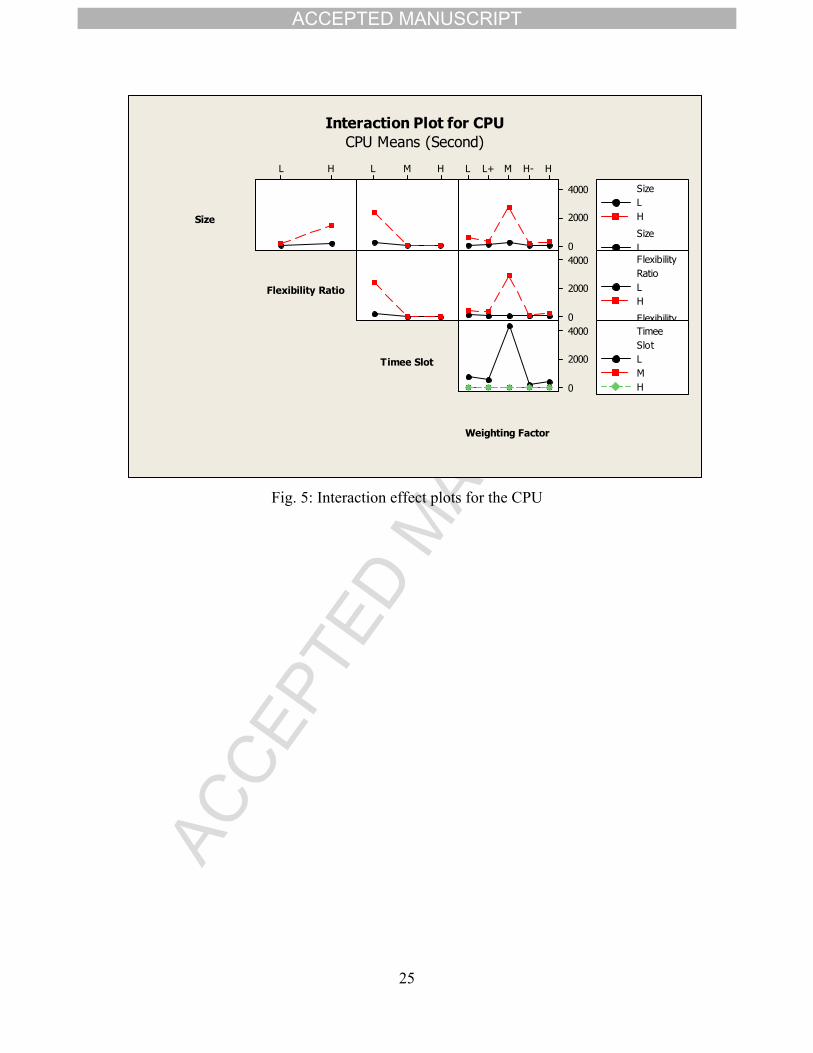
4.3.5. The interaction effect on the computation time
In order to investigate the interaction effect of the four design factors on the computation time
performance measure, the interaction plots for CPU is illustrated in Figure 5. It emerges that the
flexibility ratio slightly increases CPU for small-scale problems; however, it’s impact is significant
for the large-scale case. Also, the effect of time slot length is minimal in the small-scale case and
the low flexibility rate scenario. However, it’s effect is significant in the large-scale case and the
high flexibility ratio scenario. Furthermore, the dramatic increase in computation time is obvious
in large-scale cases, high flexibility ratio scenarios, and instances in which time slot length is low.
ACCEPTED MANUSCRIPT
25
HL HML HH-ML+L
4000
2000
04000
2000
04000
2000
0
Size
Flexibility Ratio
Timee Slot
Weighting Factor
LH
Size
LH
Size
LH
SizeLH
RatioFlexibility
LH
RatioFlexibility
LMH
SlotTimee
Interaction Plot for CPUCPU Means (Second)
Fig. 5: Interaction effect plots for the CPU

ACCEPTED MANUSCRIPT
26
Table 4: The small-scale case study numerical resultsLow Flexibility ratio High Flexibility ratio
EC EC
Comb.
#
Δt α
Cost (R) % Reduction
IC
(Slots)
CPU
(Sec.) Cost (R) % Reduction
IC (Slots) CPU
(Sec.)
1 L L 14.47 38.4 18720 42 10.44 55.5 18720 47
2 L L+ 14.47 38.4 370 71 10.44 55.5 586 522
3 L M 14.47 38.4 370 64 10.92 53.5 526 1244
4 L H- 23.05 1.8 0 59 23.05 1.8 0 194
5 L H 23.05 1.8 0 58 23.05 1.8 0 63
6 M L 14.53 38.1 3744 6 10.45 55.5 3744 11
7 M L+ 14.53 38.1 74 3 10.45 55.5 118 7
8 M M 14.53 38.1 74 3 10.45 55.5 118 8
9 M H- 14.53 38.1 74 3 10.45 55.5 118 7
10 M H 23.11 1.5 0 3 23.11 1.5 0 4
11 H L 14.89 36.6 1872 1 10.51 55.2 1872 2
12 H L+ 14.89 36.6 38 1 10.51 55.2 60 2
13 H M 14.89 36.6 38 1 10.51 55.2 60 2
14 H H- 14.89 36.6 38 1 10.51 55.2 60 2
15 H H 23.47 0.0 0 1 23.47 0.0 0 2
Average 29.9 21 40.8 141
Average Cost for the small-scale case R15.40
Average IC for the small-scale case ≈ 1690 time slots
Average CPU for the small-scale case 114 second

ACCEPTED MANUSCRIPT
27
Table 5: The large-scale case study numerical results
Low Flexibility ratio High Flexibility ratio
EC EC
Comb.
#
Δt α
Cost (R) % Reduction
IC
(Slots)
CPU
(Sec.) Cost (R) % Reduction
IC
(Slots)
CPU
(Sec.)
1 L L 31.25 53.2 37440 1062 26.29 60.6 37440 2196
2 L L+ 31.56 52.7 530 307 27.53 58.7 666 1572
3 L M 31.56 52.7 530 308 28.00 58.0 606 16168
4 L H- 38.95 41.6 200 307 37.10 44.4 220 449
5 L H 45.73 31.5 80 308 45.31 32.1 80 1294
6 M L 31.31 53.1 7488 12 26.28 60.6 7488 171
7 M L+ 31.32 53.1 158 10 26.29 60.6 294 43
8 M M 31.56 52.7 110 10 27.12 59.3 170 26
9 M H- 31.62 52.6 106 10 27.54 58.7 142 10
10 M H 45.49 31.8 16 11 44.00 34.0 16 7
11 H L 31.67 52.5 3744 3 26.34 60.5 3744 44
12 H L+ 31.68 52.5 80 3 26.35 60.5 148 8
13 H M 31.92 52.2 56 3 26.59 60.1 124 11
14 H H- 31.98 52.1 54 2 27.60 58.6 72 4
15 H H 45.55 31.7 8 3 44.36 33.5 8 3
Average 48.9 157 53.4 1467
Average Cost for the large-scale case R32.99
Average IC for the large-scale case ≈ 3370 time slots
Average CPU for the large -scale case 1215 seconds
5. Conclusion
This study discussed an experimental study of the home appliance scheduling problem that
incorporates realistic aspects. This paper has examined the factors that might affect the
scheduling of residential loads and has tested the performance of the proposed BILP
optimization model under different experimental scenarios. It has also proposed a conceptual
definition of a new parameter in the home appliances scheduling problem, the so-called
“flexibility ratio”. Furthermore, the paper presented a data set for future use in literature
pertaining to the home appliance scheduling problem. It was found that the objective function
minimized the weighted sum of electricity cost (and earned the relevant incentives) and
scheduling inconvenience.

ACCEPTED MANUSCRIPT
28
In comparison to the preferred schedule defined by the consumer, the experimental results
showed that the BILP optimization model could reduce electricity costs by around 35% (from
R23.47 to R15.4) for the small-scale case study and by around 50% (from R66.71 to R32.99) for
the large-scale case study. Numerical experiments were conducted which showed that the BILP
model solution outperforms the MINLP model solution. An electricity cost saving of 31%
compared to the schedule resulting from the MINLP model (from the literature) can be realized.
Furthermore, the BILP model reduced the computation time in a significant superior way.
Furthermore, the results showed that the problem size, flexibility ratio and objective function
weighting factor have a significant effect on EC. However, only problem size and objective
function weighting factor have a significant effect on IC. Also, the results illustrate that all four
factors have a significant interaction effect on the model computation time.
In future research, uncertainty in appliance operations time should be considered, the length
of usage duration could be different from consumer to another and from time to time. Also, non-
linearity of scheduling preferences should be modeled, i.e., by considering different preference
weights to each of the appliances at a time. Extending the model to consider multi-consumer is
an important aspect, which would enable leveling and analyzing the peak loads on a micro-grid
level. Furthermore, a dynamic load scheduling system should be developed to enable customers,
utility companies and policy makers to use it and take decisions on real-time.
References:
[1] He Y, Wang B, Wang J, Xiong W, Xia T. Residential demand response behavior analysis
based on Monte Carlo simulation: The case of Yinchuan in China. Energy. 2012 Nov
1;47(1):230-6.
[2] Alberini A, Filippini M. Response of residential electricity demand to price: The effect of
measurement error. Energy economics. 2011 Sep 1;33(5):889-95.
[3] Corno F, Razzak F. Intelligent energy optimization for user intelligible goals in smart
home environments. IEEE transactions on Smart Grid. 2012 Dec;3(4):2128-35.
[4] Electricity and heat statistics - Statistics Explained - European Commission; Available
from:
http://ec.europa.eu/eurostat/statistics-explained/index.php/Electricity_and_heat_statistics
[5] Consumption of energy - Statistics Explained - European Commission; Available from:
http://ec.europa.eu/eurostat/statistics-explained/index.php/Consumption_of_energy
ACCEPTED MANUSCRIPT
29
[6] Warren P. A review of demand-side management policy in the UK. Renewable and
Sustainable Energy Reviews. 2014 Jan 1;29:941-51.
[7] Magnago FH, Alemany J, Lin J. Impact of demand response resources on unit commitment
and dispatch in a day-ahead electricity market. International Journal of Electrical Power &
Energy Systems. 2015 Jun 1;68:142-9.
[8] U.S. Department of Energy, 2006. Benefits of Demand Response in electricity markets and
recommendations for achieving them. A Report to the Unit States Congress Pursuant to
Section 1252 of the Energy Policy Act of 2005; Available from:
https://eetd.lbl.gov/sites/all/files/publications/report-lbnl-1252d.pdf
[9] Federal Energy Regulatory Commission (FERC), 2012. Assessment of Demand Response
and Advanced Metering; Available from:
https://www.ferc.gov/legal/staff-reports/12-20-12-demand-response.pdf
[10] Benetti G, Caprino D, Della Vedova ML, Facchinetti T. Electric load management
approaches for peak load reduction: A systematic literature review and state of the art.
Sustainable Cities and Society. 2016 Jan 1;20:124-41.
[11] Meyabadi AF, Deihimi MH. A review of demand-side management: Reconsidering
theoretical framework. Renewable and Sustainable Energy Reviews. 2017 Dec 1;80:367-
79.
[12] Bari A, Jiang J, Saad W, Jaekel A. Challenges in the smart grid applications: an overview.
International Journal of Distributed Sensor Networks. 2014 Feb 6;10(2):974682.
[13] Gelazanskas L, Gamage KA. Demand side management in smart grid: A review and
proposals for future direction. Sustainable Cities and Society. 2014 Feb 1;11:22-30.
[14] Haider HT, See OH, Elmenreich W. A review of residential demand response of smart
grid. Renewable and Sustainable Energy Reviews. 2016 Jun 1;59:166-78.
[15] Wang J, Zhong H, Ma Z, Xia Q, Kang C. Review and prospect of integrated demand
response in the multi-energy system. Applied Energy. 2017 Sep 15;202:772-82.
[16] Sou KC, Weimer J, Sandberg H, Johansson KH. Scheduling smart home appliances using
mixed integer linear programming. InDecision and Control and European Control
Conference (CDC-ECC), 2011 50th IEEE Conference on 2011 Dec 12 (pp. 5144-5149).
IEEE.

ACCEPTED MANUSCRIPT
30
[17] Baldauf A. A smart home demand-side management system considering solar photovoltaic
generation. InEnergy (IYCE), 2015 5th International Youth Conference on 2015 May 27
(pp. 1-5). IEEE.
[18] Yao L, Shen JY, Lim WH. Real-Time Energy Management Optimization for Smart
Household. InInternet of Things (iThings) and IEEE Green Computing and
Communications (GreenCom) and IEEE Cyber, Physical and Social Computing
(CPSCom) and IEEE Smart Data (SmartData), 2016 IEEE International Conference on
2016 Dec 15 (pp. 20-26). IEEE.
[19] İzmitligil H, Özkan HA. A home power management system using mixed integer linear
programming for scheduling appliances and power resources. InPES Innovative Smart
Grid Technologies Conference Europe (ISGT-Europe), 2016 IEEE 2016 Oct 9 (pp. 1-6).
IEEE.
[20] Rasheed MB, Awais M, Javaid N, Iqbal Z, Khurshid A, Chaudhry FA, Ilahi F. An Energy
Efficient Residential Load Management System for Multi-Class Appliances in Smart
Homes. InNetwork-Based Information Systems (NBiS), 2015 18th International
Conference on 2015 Sep 2 (pp. 53-57). IEEE.
[21] Özkan HA. Appliance based control for home power management systems. Energy. 2016
Nov 1;114:693-707.
[22] Shirazi E, Jadid S. Cost reduction and peak shaving through domestic load shifting and
DERs. Energy. 2017 Apr 1;124:146-59.
[23] Mohseni A, Mortazavi SS, Ghasemi A, Nahavandi A. The application of household
appliances' flexibility by set of sequential uninterruptible energy phases model in the day-
ahead planning of a residential microgrid. Energy. 2017 Nov 15;139:315-28.
[24] Setlhaolo D, Xia X, Zhang J. Optimal scheduling of household appliances for demand
response. Electric Power Systems Research. 2014 Nov 1;116:24-8.
[25] Setlhaolo D, Xia X. Optimal scheduling of household appliances incorporating appliance
coordination. Energy Procedia. 2014 Jan 1;61:198-202.
[26] Setlhaolo D, Xia X. Optimal scheduling of household appliances with a battery storage
system and coordination. Energy and Buildings. 2015 May 1;94:61-70.

ACCEPTED MANUSCRIPT
31
[27] Setlhaolo D, Xia X. Combined residential demand side management strategies with
coordination and economic analysis. International Journal of Electrical Power & Energy
Systems. 2016 Jul 1;79:150-60.
[28] Logenthiran T, Srinivasan D, Shun TZ. Demand side management in smart grid using
heuristic optimization. IEEE transactions on smart grid. 2012 Sep;3(3):1244-52.
[29] Kinhekar N, Padhy NP, Gupta HO. Multiobjective demand side management solutions for
utilities with peak demand deficit. International Journal of Electrical Power & Energy
Systems. 2014 Feb 1;55:612-9.
[30] Yalcintas M, Hagen WT, Kaya A. An analysis of load reduction and load shifting
techniques in commercial and industrial buildings under dynamic electricity pricing
schedules. Energy and Buildings. 2015 Feb 1;88:15-24.
[31] Cortés-Arcos T, Bernal-Agustín JL, Dufo-López R, Lujano-Rojas JM, Contreras J. Multi-
objective demand response to real-time prices (RTP) using a task scheduling methodology.
Energy. 2017 Nov 1;138:19-31.
[32] Vaziri AM, Kamyad AV, Jajarmi A, Effati S. A global linearization approach to solve
nonlinear nonsmooth constrained programming problems. Computational & Applied
Mathematics. 2011;30(2):427-43.
[33] Eskom Tariffs & Charges 2011/12; Available from: http://www.eskom.co.za/Customer
Care/TariffsAndCharges/Documents/Tariff_brochure_20112.pdf

ACCEPTED MANUSCRIPT
Optimal load scheduling of household appliances considering consumer
preferences: an experimental analysis
Highlights
The proposed model could eliminate electricity cost by around 35% to 50%.
The proposed linear formulation can reduce the computation time in a superior
way.
Flexibility ratio has a moderate negative effect on cost function and
inconvenience.
Flexibility ratio has a significant positive effect on the computation time.
Short time-slot enlarges the problem size and has a significant impact on
computation time.