Optimal Kernel Filtering for System Identification

Jose C. PrincipeJose C. Principe

Computational NeuroEngineering Laboratory (CNEL)U i it f Fl idUniversity of Florida

principe@cnel.ufl.edu

AcknowledgmentsAcknowledgments

Dr. Weifeng Liu, Amazon

D B d Ch T i h U i iDr. Badong Chen, Tsinghua University and Post Doc CNEL

NSF ECS – 0300340, 0601271, 0964197(N i i )(Neuroengineering program)

O tliOutline

1 Introduction1. Introduction2. Least-mean-square algorithm in Kernel Space3. Kernel Affine Projection Algorithms and Recursive3. Kernel Affine Projection Algorithms and Recursive

Least Squares4. Active Learning in Kernel Filtering5. Conclusion

Wiley Book (2010)Wiley Book (2010)

Papers are available atPapers are available atwww.cnel.ufl.edu

Optimal System ID Fundamentals

System identification is regression in functional spaces: Given data pairs {u(n) d(n)} and a functional mapper y=f(u w) minimize J(e)

Optimal System ID Fundamentals

pairs {u(n),d(n)} and a functional mapper y=f(u,w), minimize J(e)Data d(n)

f(u(n) w) −

=−= 1

0)()()( N

iinuiwny

AdaptiveSystem

Data u(n) Output Error e(n)

f(u(n),w)

Cost J=E(e2(n))

Learning

Optimal solution is least squares where R is the autocorrelation matrix of the input data over the lags and p is the crosscorrelation vector between input and desired

J E(e (n))

pRw 1* −=

crosscorrelation vector between input and desired.

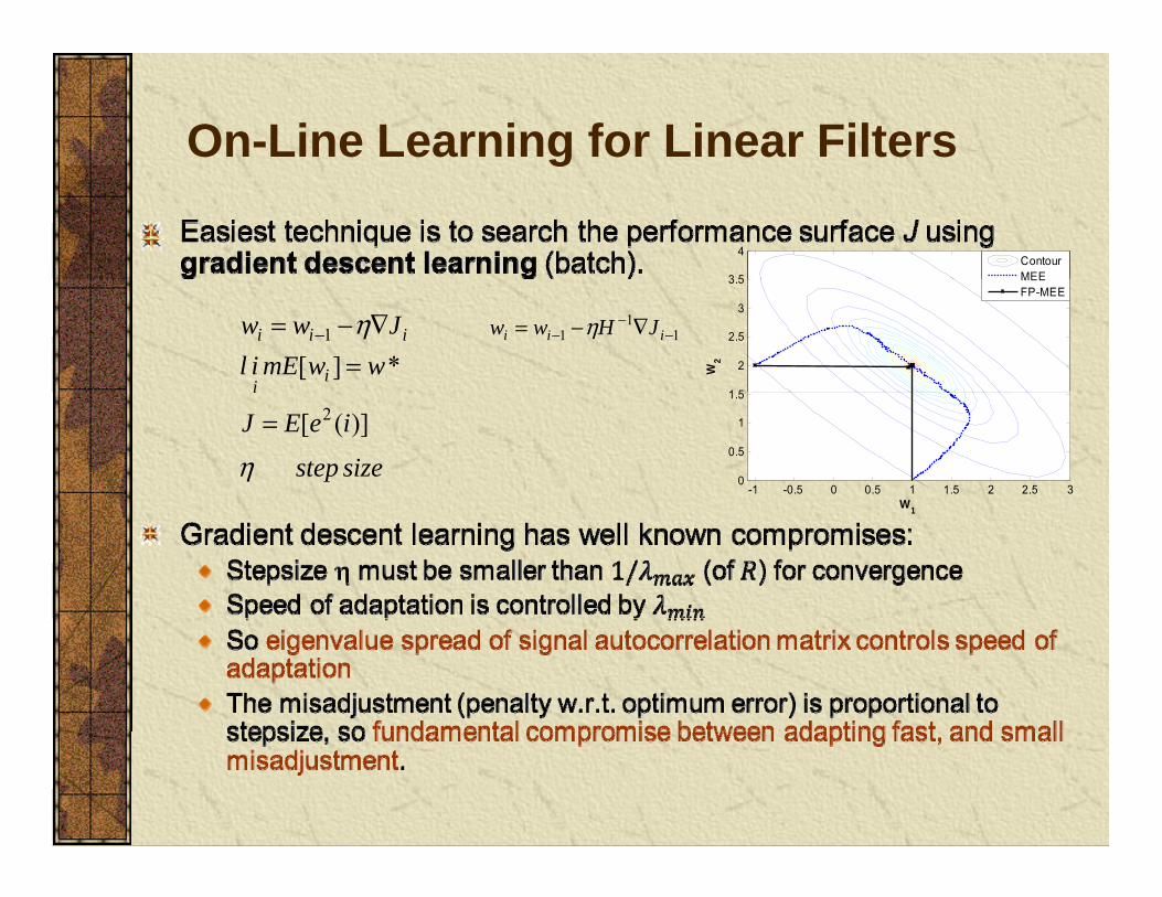
On-Line Learning for Linear Filtersg

3 5

4ContourMEE

wwmEilJww

ii

iii η*][

1

=∇−= −

W2

1 5

2

2.5

3

3.5 MEEFP-MEE

11

1 −−

− ∇−= iii JHww η

sizestep

ieEJi

η)]([ 2=

W-1 -0.5 0 0.5 1 1.5 2 2.5 3

0

0.5

1

1.5

W1

On-Line Learning for Non-Linear Filters?g

Can we generalize to nonlinear models?1i i i iw w G e−= +g

and create incrementally the nonlinear mapping?

Ty w u= ( )y f u=y pp g

( )y i

iiii eGff += −1

ifiu ( )y i

Σ( )e i

Σ

( )d i

Non-Linear Models - TraditionalNon Linear Models Traditional(Fixed topologies)

Hammerstein and Wiener modelsHammerstein and Wiener modelsAn explicit nonlinearity followed (preceded) by a linear filterNonlinearity is problem dependentDo not possess universal approximation propertyDo not possess universal approximation property

Multi-layer perceptrons (MLPs) with back-propagationNon-convex optimizationL l i iLocal minima

Least-mean-square for radial basis function (RBF) networks Non-convex optimization for adjustment of centersLocal minima

Volterra models, Recurrent Networks, etc

Non-linear Methods with Kernels

Universal approximation property (kernel dependent)Convex optimization (no local minima)Convex optimization (no local minima)Still easy to compute (kernel trick)But require regularizationSequential (On-line) Learning with KernelsSequential (On line) Learning with Kernels

(Platt 1991) Resource-allocating networksHeuristicNo convergence and well-posedness analysis

(Frieb 1999) Kernel adalineFormulated in a batch modewell-posedness not guaranteedg

(Kivinen 2004) Regularized kernel LMSwith explicit regularizationSolution is usually biased

(Engel 2004) Kernel Recursive Least Squares(Engel 2004) Kernel Recursive Least-Squares (Vaerenbergh 2006) Sliding-window kernel recursive least-squaresLiu, Principe 2008,2009, 2010.

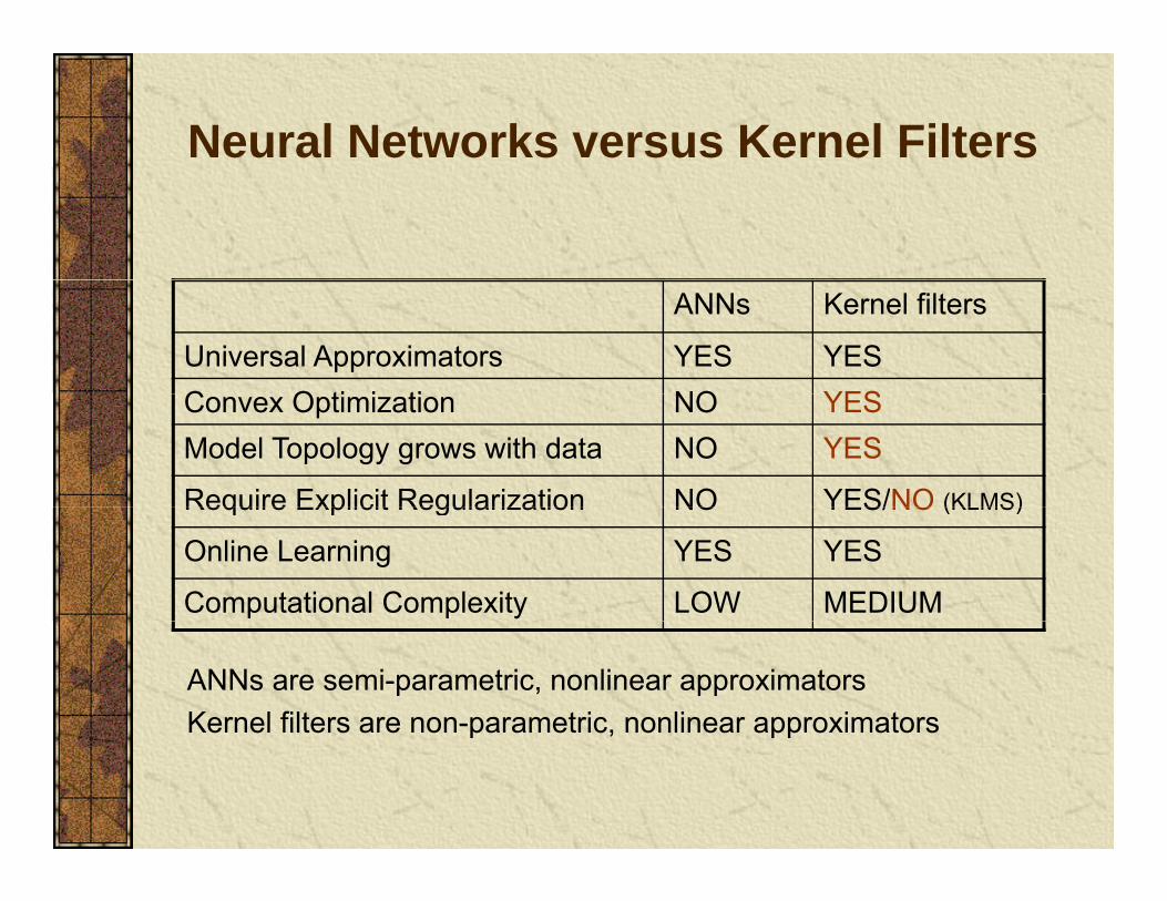
Neural Networks versus Kernel Filters

ANNs Kernel filters

Universal Approximators YES YESC O ti i ti NO YESConvex Optimization NO YESModel Topology grows with data NO YES

Require Explicit Regularization NO YES/NO (KLMS)Require Explicit Regularization NO YES/NO (KLMS)

Online Learning YES YES

Computational Complexity LOW MEDIUM

ANNs are semi-parametric, nonlinear approximatorsKernel filters are non-parametric, nonlinear approximatorsp , pp

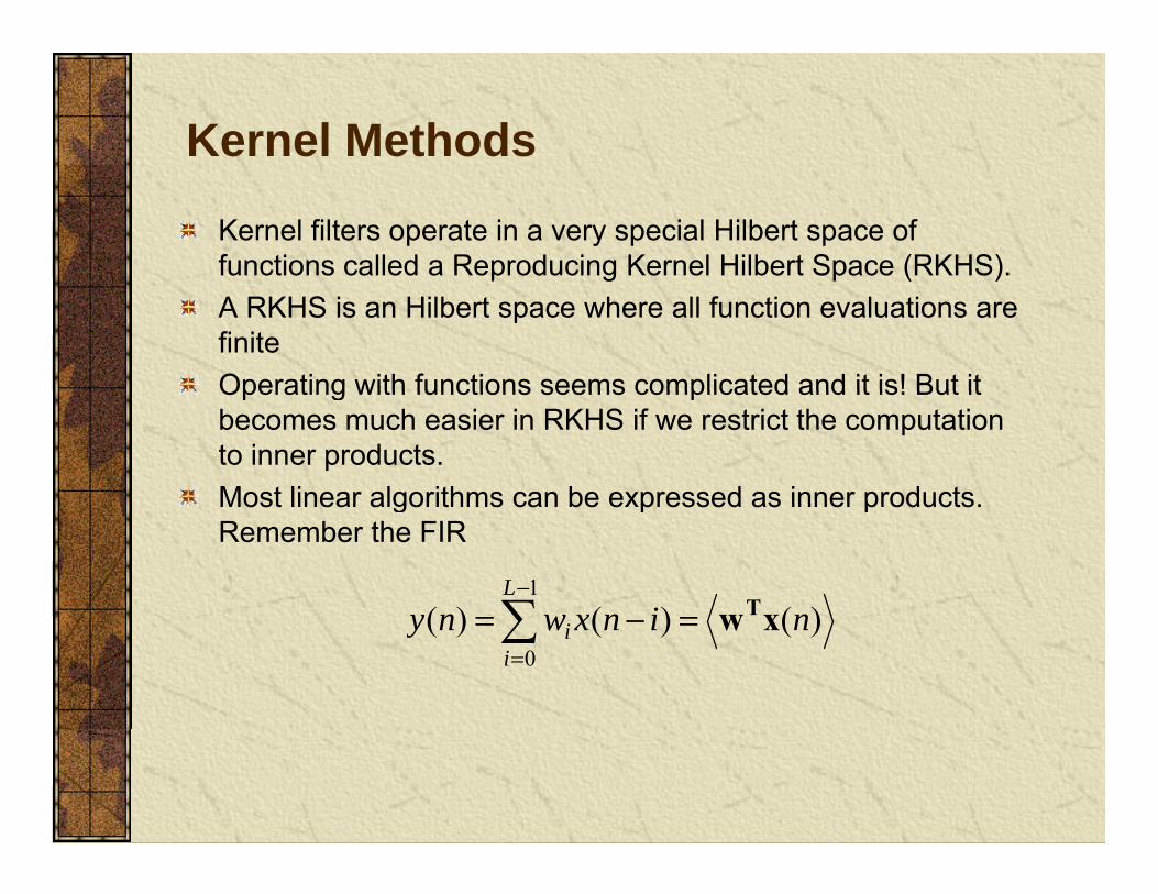
Kernel Methods

Kernel filters operate in a very special Hilbert space of functions called a Reproducing Kernel Hilbert Space (RKHS).p g p ( )A RKHS is an Hilbert space where all function evaluations are finiteOperating with functions seems complicated and it is! But itOperating with functions seems complicated and it is! But it becomes much easier in RKHS if we restrict the computation to inner products. Most linear algorithms can be expressed as inner products

)()()(1

ninxwnyL

xwT−

Most linear algorithms can be expressed as inner products. Remember the FIR

)()()(0

ninxwnyi

i xw=−==

Kernel methods

Moore-Aronszajn theoremEvery symmetric positive definite function of two real variables has a unique Reproducing Kernel Hilbert Space (RKHS).

)exp()( 2yxhyxk −−=

Mercer’s theoremLet K(x,y) be symmetric positive definite. The kernel can be

d d i th i

)exp(),( yxhyxk −−=

expanded in the series

Construct the transform as1

( , ) ( ) ( )m

i i ii

x y x yκ λϕ ϕ=

=

Inner product

( ) ( ) ( )x y x yϕ ϕ κ, = ,

1 1 2 2( ) [ ( ), ( ),..., ( )]Tm mx x x xϕ λ ϕ λ ϕ λ ϕ=

( ) ( ) ( )y yϕ ϕ, ,

Kernel methods

Mate L., Hilbert Space Methods in Science and Engineering, A. Hildger, 1989Berlinet A., and Thomas-Agnan C., “Reproducing kernel Hilbert Spaces in probaability and Statistics, Kluwer 2004

Basic idea of on-line kernel filteringg

Transform data into a high dimensional feature space Construct a linear model in the feature space F

: ( )i iuϕ ϕ=Construct a linear model in the feature space F

, ( ) Fy uϕ= Ω

Adapt iteratively parameters with gradient information

Compute the outputiii J∇−Ω=Ω − η1

p p

Universal approximation theorem 1( ) , ( ) ( , )

im

i i F j jj

f u u a u cϕ κ=

= Ω =Universal approximation theorem

For the Gaussian kernel and a sufficient large mi, fi(u) can approximate any continuous input-output mapping arbitrarily close in the Lp norm.

j

the Lp norm.

Growing network structure

1 ( ) ( )i i ie i uη ϕ−Ω = Ω +

1

1 ( ) ( , )i i if f e i uη κ−= + ⋅ mi

Kernel Least-Mean-Square (KLMS)q ( )

Least-mean-square

Transform data into a high dimensional feature space F

011 )()()( wuwidieieuww iTiiii −− −=+= η

: ( )i iuϕ ϕ=

0

1

0( ) ( ) , ( )i i Fe i d i uϕ−

Ω == − Ω 0 0

(1) (1) ( ) (1)e d u dϕΩ =

= Ω =

1 ( ) ( )i i iu e iηϕ−Ω = Ω +

( ) ( )i

jΩ

0 1

1 0 1 1 1

1 2

(1) (1) , ( ) (1)( ) (1) ( )

(2) (2) , ( )

F

F

e d u du e a u

e d u

ϕηϕ ϕ

ϕ

= − Ω =Ω = Ω + =

= − Ω

1( ) ( )i j

j

e j uη ϕ=

Ω =( ) , ( ) ( ) ( , )

i

i i F jf u u e j u uϕ η κ= Ω =

1 1 2

1 1 2

2 1 2

(2) ( ), ( )(2) ( , )

( ) (2)

Fd a u ud a u u

u e

ϕ ϕκ

ηϕ

= − = −

Ω = Ω +

RBF Centers are the samples, and Weights are the errors!1

( ) , ( ) ( ) ( , )i i F jj

f jϕ η=

1 1 2 2( ) ( )

...a u a uϕ ϕ= +

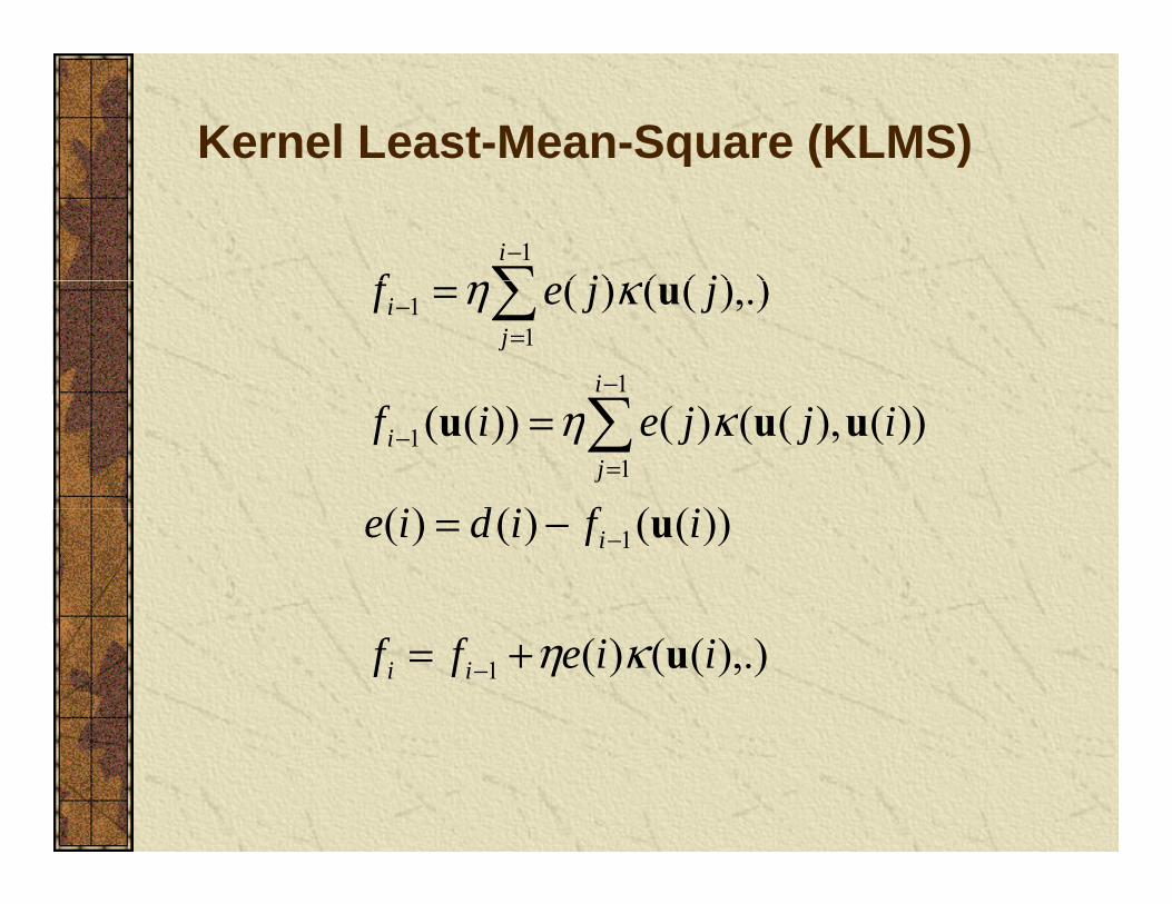
Kernel Least-Mean-Square (KLMS)( )

) )(()(1

jjfi−

),.)(()(

1

11 jjef

i

ji uκη=

−

=−

))(()()(

))(),(()())((1

1

fd

ijjeifj

i uuu κη==

− ))(()()( 1 ifidie i u−= −

),.)(()(1 iieff ii uκη+= −

Free Parameters in KLMS Initial Condition

The initialization gives the minimum possible 00 =Ω

Initial Condition

norm solution.

1

mi n nn

c P=

Ω =4

51n

3

4

1 ... 00

kς ςς ς

≥ ≥ >

2 2 2|| || || || || ||k mi c cΩ = + 1

21 ... 0k mς ς+ = = =

1 1|| || || || || ||i n nn n k

c c= = +

Ω +

0 2 4-1

0

0 2 4Liu W., Pokarel P., Principe J., “The Kernel LMS Algorithm”, IEEE Trans. Signal Processing, Vol 56, # 2, 543 – 554, 2008.

Free Parameters in KLMS Step size

T diti l i d i LMS till li hTraditional wisdom in LMS still applies here.

NN

=

=< N

jjj

Ntr

N

1))(),((][ uuG κ

ηϕ

where is the Gram matrix, and N its dimensionality.For translation invariant kernels, κ(u(j),u(j))=g0, is a

ϕG

constant independent of the data. The misadjustment is therefore ][

2 ϕη GtrN

M =

Free Parameters in KLMS Rule of Thumb for h

Although KLMS is not kernel density estimation, these rules of thumb still provide a starting point. Silverman’s rule can be applied

where σ is the input data s d R is the interquartile N{ } )5/(134.1/,min06.1 LNRh −= σ

where σ is the input data s.d., R is the interquartile, N is the number of samples and L is the dimension.Alternatively: take a look at the dynamic range of the y y gdata, assume it uniformly distributed and select h to put 10 samples in 3 σ.Use cross validation for more accurate estimationUse cross validation for more accurate estimation

Free Parameters in KLMSKernel DesignThe Kernel defines the inner product in RKHSThe Kernel defines the inner product in RKHS

Any positive definite function (Gaussian, polynomial, Laplacian, etc.) can be used. A strictly positive definite function will always yield universal mappers (Gaussian, Laplacian). For infinite number of samples all spd kernelsFor infinite number of samples all spd kernels converge in the mean to the same solution.For finite number of samples kernel function and free pparameters matter.

See Sriperumbudur et al, On the Relation Between Universality, Characteristic Kernels and RKHS Embedding ofMeasures, AISTATS 2010

SparsificationSparsification

Filter size increases linearly with samples!Filter size increases linearly with samples! If RKHS is compact and the environment stationary, we see that there is no need to keep increasing the p gfilter size.Issue is that we would like to implement it on-line! Two ways to cope with growth:

Novelty Criterion (NC)Approximate Linear Dependency (ALD)Approximate Linear Dependency (ALD)

NC is very simple and intuitive to implement.

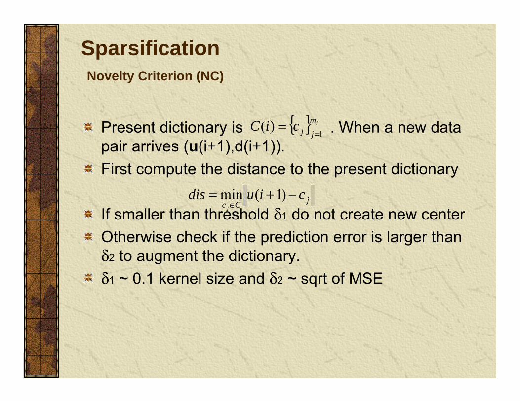
SparsificationNovelty Criterion (NC)Novelty Criterion (NC)

Present dictionary is When a new data{ } imciC )(Present dictionary is . When a new data pair arrives (u(i+1),d(i+1)).First compute the distance to the present dictionary

{ } i

jjciC1

)(=

=

p p y

If smaller than threshold δ1 do not create new centerjCc

ciudisj

−+=∈

)1(min

Otherwise check if the prediction error is larger than δ2 to augment the dictionary. δ1 0 1 kernel size and δ2 sqrt of MSEδ1 ~ 0.1 kernel size and δ2 ~ sqrt of MSE

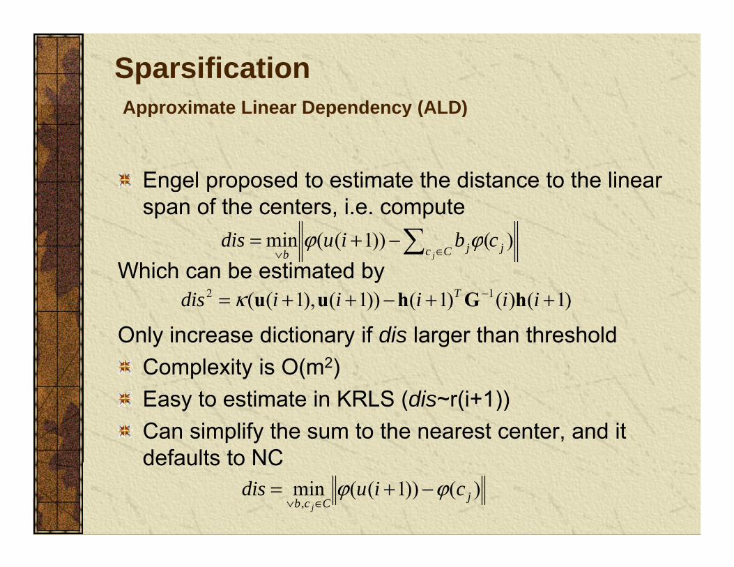
SparsificationApproximate Linear Dependency (ALD)Approximate Linear Dependency (ALD)

Engel proposed to estimate the distance to the linearEngel proposed to estimate the distance to the linear span of the centers, i.e. compute

)())1((min jC j cbiudis −+= ϕϕWhich can be estimated by

)())(( jCc jb j ∈∨

ϕϕ

)1()()1())1(),1(( 12 ++−++= − iiiiidis T hGhuuκ

Only increase dictionary if dis larger than thresholdComplexity is O(m2)E t ti t i KRLS (di (i 1))Easy to estimate in KRLS (dis~r(i+1))Can simplify the sum to the nearest center, and it defaults to NCdefaults to NC

)())1((min, jCcb

ciudisj

ϕϕ −+=∈∨

KLMS- Mackey-Glass Predictiony30

)(1)(2.0)(1.0)( 10 =

−+−+−= τττ

txtxtxtx

LMSη=0.2KLMSh=1, η=0.2

Performance Growth Trade-off

δ1=0.1, δ2=0.05η=0.1, h=1η

KLMS- Nonlinear Channel Equalization

( ) , ( ) ( ) ( , )i

i i F jf u u e j u uϕ η κ= Ω =1j =

10.5t t tz s s −= + 20.9t t tr z z nσ= − +

i ic u←( )

mi i

mi

c ua e iη

←←

Nonlinear Channel EqualizationAlgorithms Linear LMS (η=0.005) KLMS (η=0.1)

(NO REGULARIZATION)RN

(REGULARIZED λ=1)

BER (σ = 1) 0 162±0 014 0 020±0 012 0 008±0 001BER (σ = .1) 0.162±0.014 0.020±0.012 0.008±0.001

BER (σ = .4) 0.177±0.012 0.058±0.008 0.046±0.003BER (σ = .8) 0.218±0.012 0.130±0.010 0.118±0.004

Algorithms Linear LMS KLMS RN

2( , ) exp( 0.1 || || )i j i ju u u uκ = − −

Computation (training) O(l) O(i) O(i3)

Memory (training) O(l) O(i) O(i2)

Computation (test) O(l) O(i) O(i)

Memory (test) O(l) O(i) O(i)

S?Why don’t we need to explicitly regularize the KLMS?

Self-Regularization Property of KLMSg p y

Assume the data model then for any unknown vector the following inequality holds

( ) ( ) ( )oid i v iϕ= Ω +

0Ωunknown vector the following inequality holds2

111 2 2

| ( ) ( ) |1, 1,2,...,

|| || | ( ) |

i

jio

e j v jfor all i N

jη=

−−

−< =

Ω +

Ω

as long as the matrix is positive definite. SoH∞ robustness

1|| || | ( ) |o

jv jη

=Ω +

})()({ 1 TiiI ϕϕη −−

H robustness

And is upper bounded

2 1 2 2|| || || || 2 || ||oe vη−< Ω +

)(nΩAnd is upper bounded

Th l ti f KLMS i l b d d i

2 2 21|| || (|| || 2 || || )o

N vσ η ηΩ < Ω + σ1 is the largest eigenvalue of Gφ

)(nΩ

The solution norm of KLMS is always upper bounded i.e. the algorithm is well posed in the sense of Hadamard.

Liu W., Pokarel P., Principe J., “The Kernel LMS Algorithm”, IEEE Trans. Signal Processing, Vol 56, # 2, 543 – 554, 2008.

Intuition: KLMS and the Data SpacepKLMS search is insensitive to the 0-eigenvalue directions

)0()1()]([ iiE εηςε −= )0()1()]([ nnn iE εηςε2 2 2min min

0[| ( ) | ] (1 ) (| ( ) | )2 2

ii n

n n

J JE n n

η ηε ης εης ης

= + − −− −

22 )()(So if , and The 0-eigenvalue directions do not affect the MSE

2( ) [| | ]TJ i E d ϕ= − Ω

0nς = )0()]([ nn iE εε = 22 )0(])([ nn iE εε =

2 2min minmin 1 1

( ) (| (0) | )(1 )2 2

m m in n n nn n

J JJ i J

η ης ς ε ης= =

= + + − −

( ) [| | ]iJ i E d ϕ= Ω

KLMS only finds solutions on the data subspace! It does not care about the null space!

Liu W., Pokarel P., Principe J., “The Kernel LMS Algorithm”, IEEE Trans. Signal Processing, Vol 56, # 2, 543 – 554, 2008.

Tikhonov Regularization

In numerical analysis the methodology constrains the condition number of the solution matrix (or its eigenvalues)

1 2{ , ,..., }rS diag s s s=Singular value

The singular value decomposition of Φ can be written

TQS

PΦ

=

000

g

The pseudo inverse to estimate Ω in is

which can be still ill posed (very small sr) Tikhonov regularized the

00)()()( 0 iiid T νϕ +Ω=

dQP TrPI ssdiag ]0....0,,...,[ 11

1−−=Ω

s s

which can be still ill-posed (very small sr). Tikhonov regularized the least square solution to penalize the solution norm to yield

2d Ω+Ω−=Ω λTJ Φ)(1

2 21

( ,..., ,0,...,0) Tr

r

s sPdiag Q d

s sλ λΩ =

+ +Notice that if λ = 0, when sr is very small, sr/(sr

2+ λ) = 1/sr → ∞., r y , r ( r ) r

However if λ > 0, when sr is very small, sr/(sr2+ λ) = sr/ λ → 0.

Tikhonov and KLMS

In the worst case, substitute the optimal weight by the pseudo inverse

1

dQP Tr

ir

i ssdiagiE ]0....0,))1(1(,...,))1(1[()]([ 1111

−− −−−−=Ω ηςης

No regularization yields Tikhonov

2 2 1[ /( )]λ −

1ns −

0.6

0.8

1

unct

ion

PCA

2 2 1[ /( )]n n ns s sλ −+ ⋅1 if thn ns s− >

0

0.2

0.4

reg-

fu

KLMSTikhonovTruncated SVD

Regularization function for finite N in KLMS 0 if thns ≤

2 1N

0 0.5 1 1.5 2singular value

2 1[1 (1 / ) ]Nn ns N sη −− − ⋅

The stepsize and N control the reg-function in KLMS.

Liu W., Principe J. The Well-posedness Analysis of the Kernel Adaline, Proc WCCI, Hong-Kong, 2008

Energy Conservation Relation

Energy conservation in RKHS

The fundamental energy conservation relation holds in RKHS!

Energy conservation in RKHS

( ) ( )222 2 ( )( )( ) ( 1)

( ), ( ) ( ), ( )pa e ie ii i

i i i iκ κ+ = − + Ω Ω

u u u uF F

Upper bound on step size for mean square convergence

( ) ( )( ), ( ) ( ), ( )

2*2E

ΩF

0.012

St d t t f

2* 2vE

ησ

≤ +

Ω

F

F0.006

0.008

0.01

EM

SE

Steady-state mean square performance2

2lim ( )2

vai

E e i ηση→∞

= 0.002

0.004

simulationtheory

Chen B., Zhao S., Zhu P., Principe J. Mean Square Convergence Analysis of the Kernel Least Mean Square Algorithm, submitted to IEEE Trans. Signal Processing

2i η→∞ −0.2 0.4 0.6 0.8 1

0

stepsize η

Effects of Kernel Size

7

8

x 10-3

simulationtheory

0.6

0.7

0.8

σ = 0.2σ = 1.0σ = 20

4

5

6

EM

SE0.4

0.5

EM

SE

1

2

3

E

0.1

0.2

0.3

0.5 1 1.5 20

1

kernel size σ

0 200 400 600 800 10000

iteration

Kernel size affects the convergence speed! (How to choose a suitable kernel size is still an open problem)

H i d ff h fi l i dj ! ( i lHowever, it does not affect the final misadjustment! (universal approximation with infinite samples)

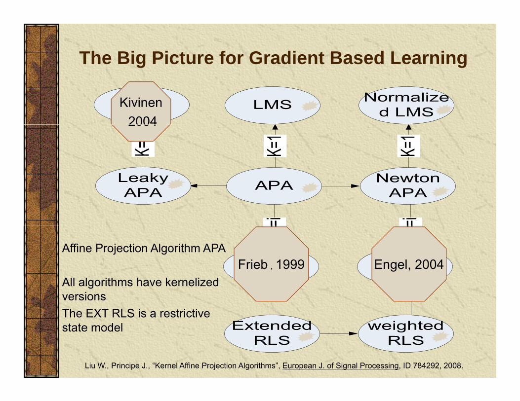
The Big Picture for Gradient Based Learning

Kivinen20042004

Frieb , 1999 Engel, 2004Affine Projection Algorithm APA

All algorithms have kernelizedversionsThe EXT RLS is a restrictive state modelstate model

Liu W., Principe J., “Kernel Affine Projection Algorithms”, European J. of Signal Processing, ID 784292, 2008.

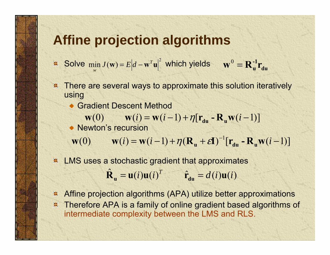
Affine projection algorithmsp j gSolve which yields 2

)(min uww T

wdEJ −= du

-1u rRw =0

There are several ways to approximate this solution iteratively using

Gradient Descent Method

Newton’s recursion )]1([)1()()0( −+−= iii wR-rwww uduη

)]1([)()1()()0( 1 −++−= − iii wR-rIRwww dεη

LMS uses a stochastic gradient that approximates

)]1([)()1()()0( ++ iii wRrIRwww uduu εη

)()(ˆ)()(ˆ iidii T uruuR ==

Affine projection algorithms (APA) utilize better approximationsTherefore APA is a family of online gradient based algorithms of

)()()()( iidii uruuR duu ==

y g gintermediate complexity between the LMS and RLS.

Affine projection algorithmsp j gAPA are of the general form

TidKidiiKii )]()1([)()]()1([)( +−=+−= duuU LxK idKidiiKii )](),...,1([)()](),...,1([)( +−=+−= duuU

)()(1ˆ)()(1ˆ iiK

iiK

T dUrUUR duu ==

Gradient

KK

)]1()()()()1()()0( −+−= iiiiii T wU-[dUwww η

Newton

Notice that)]1()()()[())()(()1()( 1 −++−= − iiiiiiii TT wU-dUIUUww εη

Notice that

So11 ))()()(()())()(( −− +=+ IUUUUIUU εε iiiiii TT

)]1()()([])()()[()1()( 1 −++−= − iiiiiiii TT wU-dIUUUww εη

Affine projection algorithmsp j gIf a regularized cost function is preferred

22)(i λTdEJ

The gradient method becomes

)(min wuww λ+−= T

wdEJ

g

)]1()()()()1()1()()0( −+−−= iiiiii T wU-[dUwww ηηλ

Newton

Or)()())()(()1()1()( 1 iiiiii T dUIUUww −++−−= εηηλ

Or

)(])()()[()1()1()( 1 iiiiii T dIUUUww −++−−= εηηλ

Kernel Affine Projection Algorithmsj g

KAPA 1 2 use the least squares cost while KAPA 3 4 are regularized

Ω≡wQ(i)

KAPA 1,2 use the least squares cost, while KAPA 3,4 are regularizedKAPA 1,3 use gradient descent and KAPA 2,4 use Newton updateNote that KAPA 4 does not require the calculation of the error by

iti th ith th t i i i l d i threwriting the error with the matrix inversion lemma and using the kernel trick

Note that one does not have access to the weights, so need recursion i KLMSas in KLMS.

Care must be taken to minimize computations.

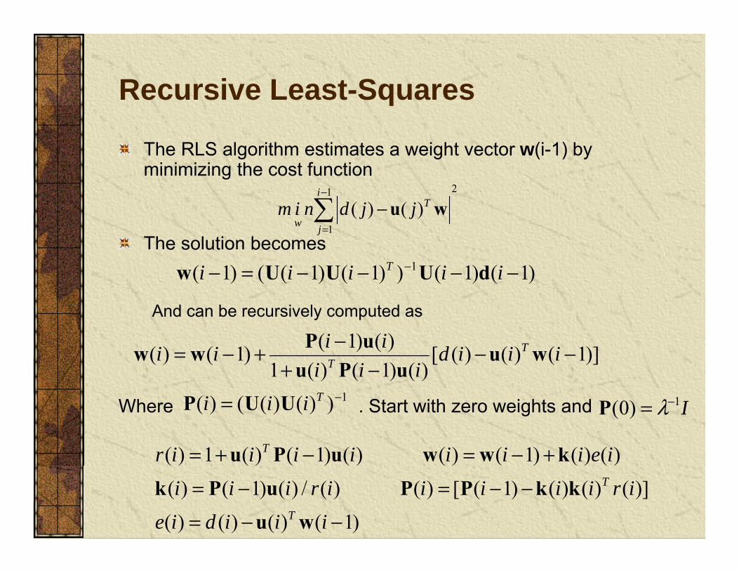
Recursive Least-Squaresq

The RLS algorithm estimates a weight vector w(i-1) by minimizing the cost functiong

The solution becomes

21

1)()(

−

=

−i

j

T

wjjdnim wu

e so ut o beco es

And can be recursively computed as

)1()1())1()1(()1( 1 −−−−=− − iiiii T dUUUw

)]1()()([)()1()(1

)()1()1()( −−−+

−+−= iiidiii

iiii TT wu

uPuuPww

1TWhere . Start with zero weights and

)()()1()()()1()(1)( +−=−+= ieiiiiiiir T kwwuPu

1))()(()( −= Tiii UUP I1)0( −= λP

)1()()()()]()()()1([)()(/)()1()(

−−=−−=−=

iiidieiriiiiiriii

T

T

wukkPPuPk

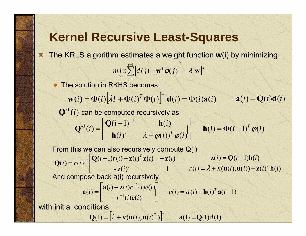
Kernel Recursive Least-SquaresqThe KRLS algorithm estimates a weight function w(i) by minimizing

221

)()( ww λϕ +−−i

T jjdnim

The solution in RKHS becomes 1

)()( ϕ=jw

jj

[ ] )()()()()()()( 1 iiiiiIii T adw Φ=ΦΦ+Φ= −λ )()()( iii dQa =can be computed recursively as

[ ] )()()()()()()()(i-1Q

)()1()()())()(

)()1()(

1

iiiiii

iii T

TTϕ

λ−Φ=

−=

−

hh

hQQ-1

From this we can also recursively compute Q(i) )()1()()()()()()1(

)()( 1 iiiiiiiriiri

T hQzzzzQQ

−=

−+−

= −

)())()( iii TT ϕϕλ

+h

And compose back a(i) recursively )()())(),(()(1)(

)()(iiiiiri

iri TT hzuuz-Q

−+=

=κλ

)1()()()()()()()(

)(1

−−=

−

=−

iiidieieirii

i T ahza

a

with initial conditions

)1()()()()()(

)( 1 =

=−

iiidieieir

i aha

[ ] )1()1()1(,))(),(()1( 1 dii T QauuQ =+= −κλ

KRLS

)()( 1 ieira

uc

mi

imi−←

←

1

)()()( 1 iieiraa jjmijmi z−−− −←

1

2

1

2

mi-1

mimi-1

mi )),(()()(1

uuau jifi

ji κ

=

=1j=

Engel Y., Mannor S., Meir R. “The kernel recursive least square algorithm”, IEEE Trans. SignalProcessing, 52 (8), 2275-2285, 2004.

KRLS

[ ] )()),(()()),(()( 1

11

1 iejiiirff i

j jii ⋅−⋅+= −

=−

− uzu κκ

)()()( 1 ieirii = −a

)}(),1({)(

1,...,1)()()()()( 1

iuiCiC

ijiieirii jjj

−=

−=−= − zaa

Computation complexityy

Prediction of Mackey GlassPrediction of Mackey-Glass

L 10L=10K=10K=50 SW KRLSK=50 SW KRLS

Simulation 1: Noise Cancellationn(i) ~ uniform [-0.5, 05]

( ) ( ) 0.2 ( 1) ( 1) ( 1) 0.1 ( 1) 0.4 ( 2)u i n i u i u i n i n i u i= − − − − − + − + −( ( ), ( 1), ( 1), ( 2))H n i n i u i u i= − − −

Simulation 1: Noise Cancellation

2( ( ) ( )) exp( || ( ) ( ) || )u i u j u i u jκ =( ( ), ( )) exp( || ( ) ( ) || )u i u j u i u jκ = − −

K=10

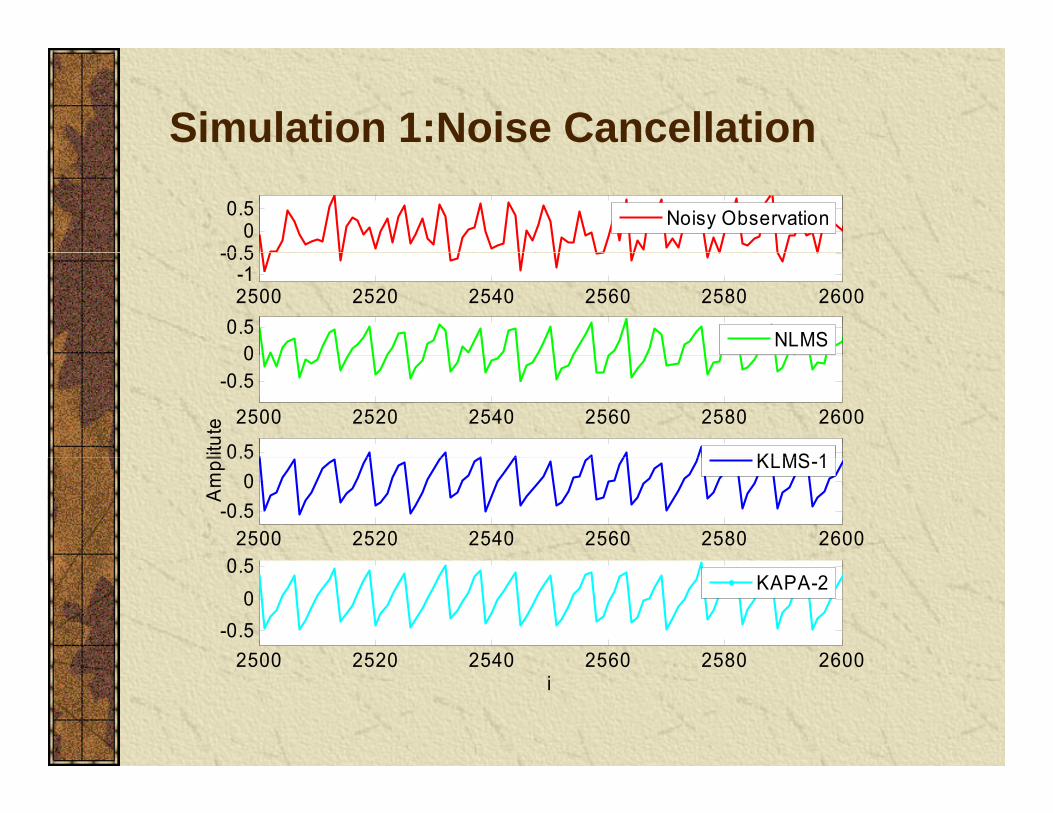
Simulation 1:Noise Cancellation

0 50

0.5

Noisy Observation

2500 2520 2540 2560 2580 2600-1

-0.5

00.5

NLMS

2500 2520 2540 2560 2580 2600

-0.50

0.5

KLMS 1litut

e

2500 2520 2540 2560 2580 2600-0.5

00.5

KLMS-1

0 5

Am

pl

2500 2520 2540 2560 2580 2600-0.5

00.5

KAPA-2

2500 2520 2540 2560 2580 2600i

Simulation-2: nonlinear channel equalization

10.5t t tz s s −= + 20.9t t tr z z nσ= − +

K=100 1σ=0.1

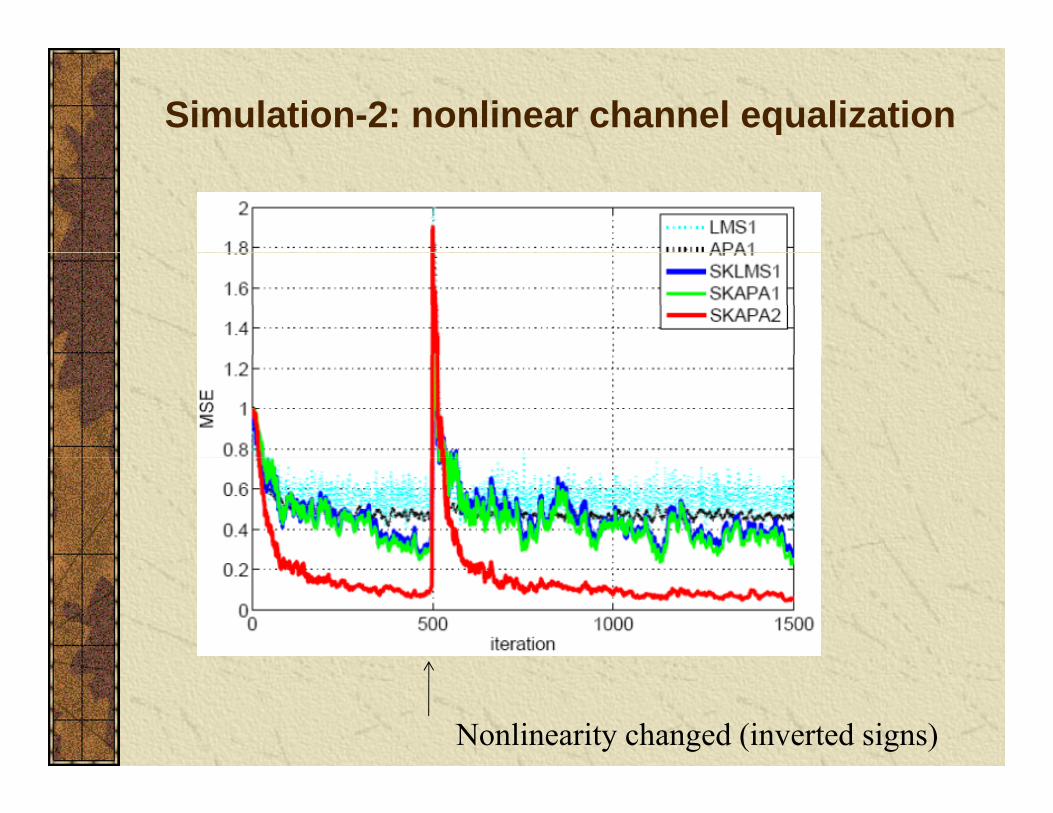
Simulation-2: nonlinear channel equalization

Nonlinearity changed (inverted signs)

Active Data Selection

Is the Kernel trick a “free lunch”?Is the Kernel trick a free lunch ?

The price we pay is large memory to store centers P i t i l ti f th f tiPointwise evaluations of the function

But remember we are working on an on-line scenario, so most of the methods out there need to be modified.

Active Data Selection

The goal is to build a constant length (fixed budget)The goal is to build a constant length (fixed budget) filter in RKHS. There are two complementary methods of achieving this goal:

Discard unimportant centers (pruning)Accept only some of the new centers (sparsification)

Apart from heuristics, in either case a methodology to evaluate the importance of the centers for the overall pnonlinear function approximation is needed.Another requirement is that this evaluation should be no more expensive computationally than the filterno more expensive computationally than the filter adaptation.

Previous Approaches – Sparsificationpp pNovelty condition (Platt, 1991)

• Compute the distance to the current dictionaryCompute the distance to the current dictionary

• If it is less than a threshold δ1 discardIf the prediction error

jiDcciudis

j

−+=∈

)1(min)(

• If the prediction error

• Is larger than another threshold δ2 include new center. )()1()1()1( iiidie T Ω+−+=+ ϕ

Approximate linear dependency (Engel, 2004)• If the new input is a linear combination of the previous

centers discardcenters discard

which is the Schur Complement of Gram matrix and fits KAPA 2 d 4 ll P bl i t ti l l it

∈−+=

)(2 )()1((miniDc jj

jcbiudis ϕϕ

and 4 very well. Problem is computational complexity

Previous Approaches – Pruningpp gSliding Window (Vaerenbergh, 2010)

Impose mi<B in =im

jji ciaf )()( κImpose mi<B in Create the Gram matrix of size B+1 recursively from size B

=+)(

)1(hiG

iG

=j

jji ciaf1

,.)()( κ

[ ]TBBB cccch ),(),...,,( 111 ++= κκ

=+++ ),(

)1(11 BB

T cchiG

κhzccrhiQziGIiQ T

BB −+==+= ++− ),()())(()( 11

1 κλλ +iQ T //)(

Downsize: reorder centers and include last (see KAPA2)

−−+

=+rrzrzrzziQ

iQ T

T

/1///)(

)1(

See also the Forgetron and the Projectron that provide error bounds for the approximation

=+ +=++=+−=+ B

j jjiT ciafidiQiaeffHiQ

11 ,.)()1()1()1()1(/)1( κ

error bounds for the approximation. O. Dekel, S. Shalev-Shwartz, and Y. Singer, “The Forgetron: A kernel-based perceptron on a fixed budget,” in Advancesin Neural Information Processing Systems 18. Cambridge, MA: MIT Press, 2006, pp. 1342–1372.F. Orabona, J. Keshet, and B. Caputo, “Bounded kernel-based online learning,” Journal of Machine Learning Research,vol. 10, pp. 2643–2666, 2009.

Information Theoretic Statement

Th l i t ))(( iTThe learning systemAlready processed (the dictionary)

))(;( iTuy

ijdjuiD )}()({)( =

A new data pair How much new information it contains?

jjdjuiD 1)}(),({)( ==)}1(),1({ ++ idiu

How much new information it contains?Is this the right question? NOHow much information it contains with respect to theHow much information it contains with respect to the

learning system ?))(;( iTuy

Information Measure

Hartley and Shannon’s definition of informationHow much information it contains?

))1(),1((ln)1( ++−=+ idiupiI

Learning is unlike digital communications:The machine never knows the joint distribution!

When the same message is presented to a learning system information (the degree of uncertainty) changes because the system learned with the first g ypresentation! Need to bring back MEANING into information theory!

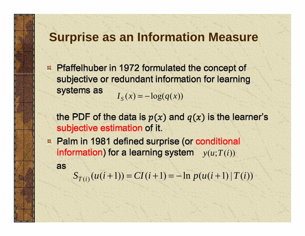
Surprise as an Information Measurep

Learning is very much like an experiment that we do in the laboratory. Fedorov (1972) proposed to measure the importance of an experiment as the Kulback Leibler distanceof an experiment as the Kulback Leibler distance between the prior (the hypothesis we have) and the posterior (the results after measurement).Mackay (1992) formulated this concept under a Bayesian approach and it has become one of the key concepts in active learningconcepts in active learning.

Surprise as an Information Measurep

))(log()( xqxIS −=

))(;( iTuy

))(|)1((ln)1())1(()( iTiupiCIiuS iT +−=+=+

Shannon versus Surprise

Shannon SurpriseShannon (absolute

information)

Surprise (conditional information)

Objective Subjective

Receptorindependent

Receptor dependent (on time

and agent)g )Message is

meaninglessMessage has

meaning for the agentagent

Evaluation of Conditional Information (surprise)

Gaussian process theoryGaussian process theory

))1(ˆ)1((

))](|)1(),1((ln[)1(2idid

iTidipiCI

++

=++−=+ u

where

))](|)1((ln[)1(2

))1()1(()1(ln2ln 2 iTipi

ididi +−+

+−++++ uσ

σπ

)()]([)1()1(ˆ1222

12 ++=+ − idiiidT

nT GIh σ

)1()]([)1())1(),1(()1( 1222 +++−+++=+ − iiiiii nT

n hGIhuu σκσσ

Interpretation of Conditional Information (surprise)(surprise)

ˆ))](|)1(),1((ln[)1(

2

iTidipiCI =++−=+ u

))](|)1((ln[)1(2

))1(ˆ)1(()1(ln2ln 2

2

iTipi

ididi +−+

+−++++ uσ

σπ

Prediction errorLarge error large conditional information

Prediction variance

)1(ˆ)1()1( +−+=+ ididie

)1(2 +iσPrediction varianceSmall error, large variance large CILarge error, small variance large CI (abnormal)

I t di t ib ti

)1( +iσ

))(|)1(( iTip +uInput distributionRare occurrence large CI

))(|)1(( iTip +u

Redundant, abnormal and learnable

1)1(: TiSAbnormal >+ 1

)1(

)(

TiSTL bl ≥≥ 21 )1(: TiSTLearnable ≥+≥

2)1(:Re TiSdundant <+

Still need to find a systematic way to select these thresholds which are hyperparameters.

Simulation-5: KRLS-SC nonlinear regression

Nonlinear mapping is y=-x+2x2+sin x in unit variance Gaussian noise

Simulation-5: nonlinear regression–5% most surprising data5% most surprising data

Simulation-5: nonlinear regression—redundancy removal

Simulation-5: nonlinear regressiong

Simulation-6: nonlinear regression—abnormality detection (15 outliers)

KRLS-SC

Simulation-7: Mackey-Glass time series prediction

Simulation-8: CO2 concentration forecasting

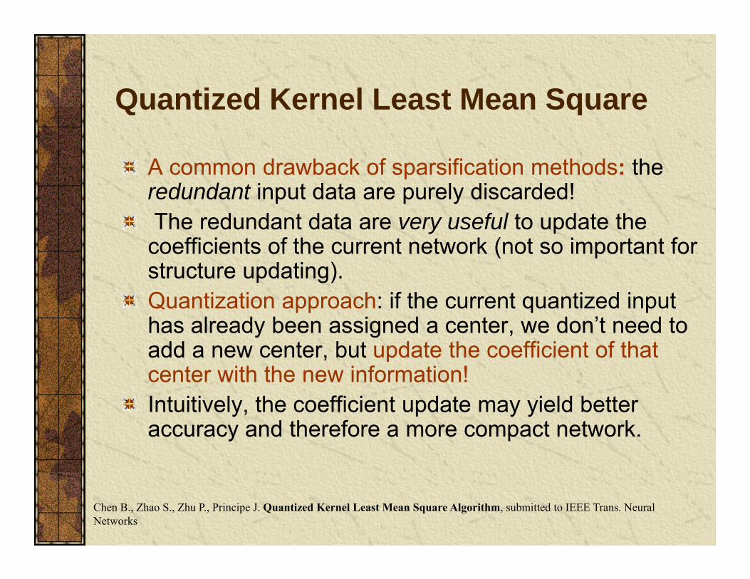
Quantized Kernel Least Mean SquareQuantized Kernel Least Mean Square

A common drawback of sparsification methods: the redundant input data are purely discarded!The redundant data are very useful to update the coefficients of the current network (not so important forcoefficients of the current network (not so important for structure updating). Quantization approach: if the current quantized input has already been assigned a center we don’t need tohas already been assigned a center, we don t need to add a new center, but update the coefficient of that center with the new information!I t iti l th ffi i t d t i ld b ttIntuitively, the coefficient update may yield better accuracy and therefore a more compact network.

Chen B., Zhao S., Zhu P., Principe J. Quantized Kernel Least Mean Square Algorithm, submitted to IEEE Trans. Neural Networks

Quantized Kernel Least Mean SquareQuantized Kernel Least Mean Square

Quantization in Input Space 0 0f =p p

[ ]( )1

1

( ) ( ) ( ( ))

( ) ( ) ,i

i i

e i d i f i

f f e i Q iη κ−

−

= − = +

u

u .

Quantization in RKHS (0) =

0Ω

[ ]( ) ( ) ( 1) ( )( ) ( 1) ( ) ( )

Te i d i i ii i e i iη

= − − = − +

ΩΩ Ω

ϕϕQ

Using the quantization method to

compress the input (or feature) space

[ ]( ) ( ) ( ) ( )η ϕ

and hence to compact the RBFstructure of the kernel adaptive filter

Quantization operator

Quantized Kernel Least Mean Squareq

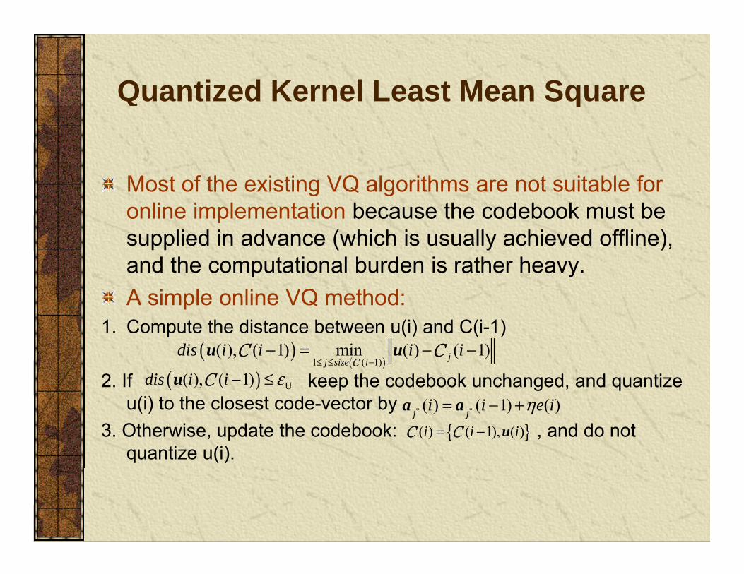
M t f th i ti VQ l ith t it bl fMost of the existing VQ algorithms are not suitable for online implementation because the codebook must be supplied in advance (which is usually achieved offline), and the computational burden is rather heavy. A simple online VQ method:

1 Compute the distance between u(i) and C(i 1)1. Compute the distance between u(i) and C(i-1)

2. If keep the codebook unchanged, and quantize ( )

( )1 ( 1)( ), ( 1) min ( ) ( 1)jj size i

dis i i i i≤ ≤ −

− = − −u uC

C C

( )( ), ( 1)dis i i ε− ≤u UC

u(i) to the closest code-vector by 3. Otherwise, update the codebook: , and do not

quantize u(i). { }( ) ( 1), ( )i i i= − uC C

* *( ) ( 1) ( )j j

i i e iη= − +a a

Quantized Kernel Least Mean SquareQuantized Kernel Least Mean Square

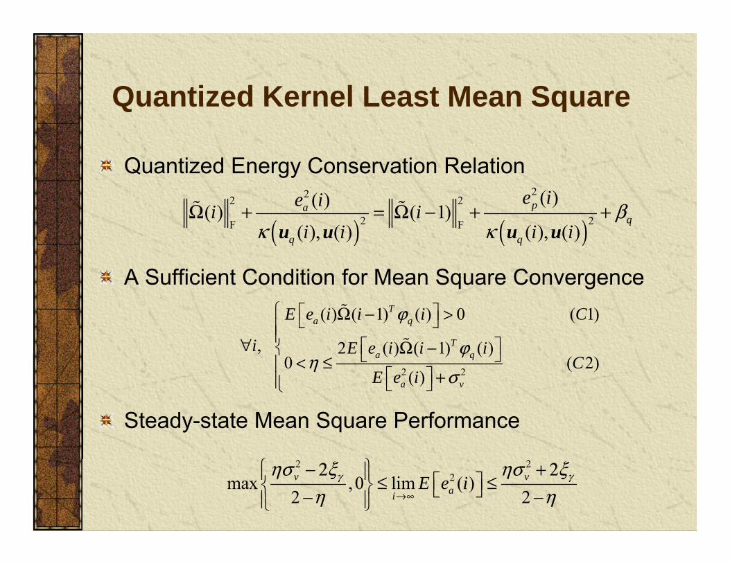
Quantized Energy Conservation Relationgy

( ) ( )222 2

2 2

( )( )( ) ( 1)( ), ( ) ( ), ( )

paq

q q

e ie ii ii i i i

βκ κ

+ = − + + Ω Ωu u u uF F

A Sufficient Condition for Mean Square Convergence ( ) ( 1) ( ) 0 ( 1)TE e i i i C − >

Ω ϕ

2 2

( ) ( 1) ( ) 0 ( 1)

, 2 ( ) ( 1) ( )0 ( 2)

( )

a q

Ta q

a v

E e i i i C

i E e i i iC

E e iη

σ

> ∀ − < ≤ +

Ω

Ω

ϕ

ϕ

Steady-state Mean Square Performance

2 22max ,0 lim ( )

2 2v v

aiE e iγ γησ ξ ησ ξ

η η→∞

− + ≤ ≤ − −

2 2

Quantized Kernel Least Mean SquareQuantized Kernel Least Mean Square

Static Function Estimation2 2( ( ) 1) ( ( ) 1)( ) 0.2 exp exp ( )

2 2u i u id i v i

+ −= × − + − +

Upper bound 30

40

10-1

EM

SE

pp

20

netw

ork

size

EMSE = 0.017110

final

n

10-2 10-1 100 10110-2

quantization factor γ

Lower bound

2 4 6 8 100.10

quantization factor γ

Quantized Kernel Least Mean SquareQuantized Kernel Least Mean Square

Short Term Lorenz Time Series Prediction

500101

QKLMS

350

400

450

e

100

SE

NC-KLMSSC-KLMS

150

200

250

300

netw

ork

siz

QKLMSNC-KLMSSC-KLMS

10-1

test

ing

MS

0 1000 2000 3000 40000

50

100

150

0 1000 2000 3000 400010-3

10-2

0 1000 2000 3000 4000iteration

0 1000 2000 3000 4000iteration

Quantized Kernel Least Mean SquareQuantized Kernel Least Mean Square

Short Term Lorenz Time Series Prediction

350

400

QKLMSNC-KLMS

101

QKLMSNC-KLMS

250

300

size

SC-KLMS

100

SE

SC-KLMSKLMS

100

150

200

netw

ork

s

-2

10-1

test

ing

M

0 1000 2000 3000 40000

50

100

0 1000 2000 3000 4000

10-3

10 2

0 1000 2000 3000 4000

iteration0 1000 2000 3000 4000

iteration

Generality of the Methods Presented

The methods presented are general tools for designingThe methods presented are general tools for designing optimal universal mappings, and they can be applied in statistical learning.g

Can we apply online kernel learning for Reinforcement learning? Definitely YES. g yCan we apply online kernel learning algorithms for classification? Definitely YES. yCan we apply online kernel learning for more abstract objects, such as point processes or graphs? Definitely j , p p g p yYES

Redefinition of On-line Kernel Learning

Notice how problem constraints affected the form of theNotice how problem constraints affected the form of the learning algorithms.

On-line Learning: A process by which the freeOn line Learning: A process by which the free parameters and the topology of a ‘learning system’ are adapted through a process of stimulation by the p g p yenvironment in which the system is embedded.

Error-correction learning + memory-based learningg y gWhat an interesting (biological plausible?) combination.

Impacts on Machine Learning

KAPA algorithms can be very useful in large scale g y glearning problems.

Just sample randomly the data from the data base and p yapply on-line learning algorithms

There is an extra optimization error associated with pthese methods, but they can be easily fit to the machine contraints (memory, FLOPS) or the processing time constraints (best solution in x seconds).