Optimal Inter-Release Time between Sequentially Released Products*

Jackie Y. Luan Tuck School of Business at Dartmouth

100 Tuck Hall Hanover, NH 03755-9000

Email: jackie.luan@tuck.dartmouth.edu Phone: 603-646-8136

K. Sudhir Yale School of Management

135 Prospect Street, PO Box 208200 New Haven, CT 06520

Email: k.sudhir@yale.edu Phone: 203-432-3289

This draft: September 2006

* This paper is part of the first author’s doctoral dissertation at Yale University. The authors thank seminar participants at Dartmouth College, New York University, Northwestern University, SUNY at Buffalo, University of California, Berkeley, University of Texas at Austin, University of Tortonto, Washington University at St. Louis and Yale University. The authors also thank Dina Mayzlin, Subrata Sen and Jiwoong Shin for their comments.

1

Optimal Inter-Release Timing for Sequentially Released Products

Abstract

Marketers routinely use timing as a segmentation device through sequential product releases.

While there has been much theoretical research on the optimal introduction strategy of

sequential releases, there is little empirical research on this problem. This paper develops an

econometric model to empirically solve the inter-release timing problem: it involves (1)

developing and estimating a structural model of consumers’ choice for sequentially released

products and (2) using the estimates of the structural model to solve for the optimal inter-release

time.

The empirical application focuses on the motion industry, where we specifically address the

issue of the inter-release time between a theatrical movie and its DVD version — a topic of

great managerial relevance to Hollywood studios. The results from model estimation and policy

analysis yield a number of interesting insights. In particular, we find that, given the consumer

preferences and industry cost structure in our sample, the theater-DVD window that maximizes

the industry revenue is about 2.5 months for an average movie.

2

1. Introduction

Marketers routinely use timing as a segmentation device through sequential product releases.

Customers who want to use a product early generally tend to value them more and therefore are

willing to pay more. For example, publishing companies conventionally release hardcover

version of a book first at a higher price and follow it up with the lower-quality, lower-priced

paperback version approximately one year later. Camera manufacturers often introduce a

high-end version of cameras targeted at professional users many months before introducing a

lower-end version based on the same core technology. In the motion picture industry, a movie

opens first in movie theaters, and is released in the home video market a few months later.

A central question facing these managers is the following: when firms seek to implement a

segmentation strategy with release timing as their main segmentation tool, what should be the

optimal inter-release time? The problem has been of general interest to marketers in a wide

range of industries such as publishing, electronics and entertainment (e.g., Moorthy and Png

1992; Lehmann and Weinberg 2000). Recently, the problem has gained considerable attention

in the context of the movie-DVD release timing. Since the DVD technology was commercially

introduced in 1997, the revenue stream from DVD sales and rentals has become pivotal for

studios’ financial performance in recent years. In 2004, while the US box-office gross remained

stagnant at about $9 billion, DVD rental and sales rapidly expanded to over $21 billion, making

the DVD market twice as large as the theatrical exhibition market. The enormous growth of the

DVD market has disrupted the traditional revenue structure and channel relationships in the

industry, and raises a number of questions both of practical significance and of scholarly interest;

in particular, whether and how studios should modify the conventional theater-to-DVD window

to adapt to the reality that there is greater revenue downstream.1 The average movie-DVD

release timing has been steadily shortening over the last eight years from about 7 months in

1998 to about 4.5 months in 2005. The increasingly shrinking window has sparked much

controversy within the movie industry.2

1 The applicability of the model may well go beyond the theater and DVD stages and extend to other stages of a typical Hollywood movie’s sequential release scheme, such as pay-per-view (PPV), video-on-demand (VOD), premium channel premiere and network TV showing. We focus on the issue of theater-DVD window to simplify the conceptual underpinnings of the econometric approach. Currently, the theatrical and DVD markets combined account for over 90% of the movie-related revenue. 2 While many executives including the President of Universal Studios Rick Finkelstein, perceive that this trend of shortening DVD releases has “gone too far,” others such as Disney have proposed shortening the movie-DVD window to a 4 month standard. At the extreme, Mark Cuban of 29/29 Entertainment has advocated a simultaneous release of movies and DVDs. In fact Mark Cuban’s studio recently released Steven Soderbergh’s “Bubble” in

3

Despite the importance of the inter-release timing issue across a wide range of industries

and the especially heated arguments in the movie industry, there is little research that allows us

to address this problem in an empirically grounded fashion. Our goal in this paper is to develop

a structural consumer choice model that accounts for the tradeoffs in consumers’ decisions

towards sequentially released products, which would then enable us to solve for the optimal

inter-release time in an empirical manner. Our empirical application is in the context of

movie-DVD inter-release time.

We begin by considering the tradeoffs faced by managers as they decide on the optimal

inter-release time. First, managers would like to reap the gains from both markets as quickly as

possible (money today is better than money tomorrow) so would like to shrink the inter-release

time. However, moving up the second release would cannibalize the sales of the first (and

higher-margin) product because, after the second product is released, many customers who

would otherwise purchase the higher-end version would switch to the lower-margin version.

This is the tradeoff that has been modeled in Lehmann and Weinberg (2000). However, there

two other major factors which needs to be accounted in deciding inter-release times for

sequential releases.

First, we need to model how buzz spills over from the initial release to the subsequent

release and how this is affected by the inter-release time. Many products like books and movies

receive considerable critical attention, advertising support, and media coverage as they are

initially released in hardcover or in movie theaters. These buzz effects not only affect the initial

release but also the subsequent release. Another source of buzz is the word-of-mouth that comes

from people experiencing the initial release. However the buzz effect tends to decay over time

for most products. And it is widely recognized in the context of entertainment products like

movies and DVDs. As one studio executive put it, “Movies are like fresh fish; they become stale

if you don’t sell it fast.” Another studio executive compared movies to ice cubes – “The longer

it sits, the smaller it becomes.” Hence the loss from a delayed second release not simply comes

from time discounting, but, more importantly, from the lower sales potential for the second

theaters only four days before it became available on DVD, but the movie proved to be a small-scale experiment since it was boycotted by major theater chains.

4

release due to the buzz decay. We need to empirically measure the extent of buzz decay and the

effect of inter-release window on the potential of the subsequent release in our empirical work.3

Second, shortening the inter-release time has a dynamic impact on consumer choice. Even

before the second product is released, forward-looking customers are likely to delay their

purchases and wait for the lower-priced version if they expect the second product to become

available sooner. Now that the decision to delay is related to customer expectations of

inter-release times, understanding the determinants of these expectations is important as well.

There is empirical evidence that consumers are indeed forward-looking when faced with

choices over time. For example, Weiss (1994) use questionnaire data from firms to support the

hypothesis that the firms that expect the next generation of technology to be available sooner are

more likely to defer their adoption of the currently best technology. Boone et al. (2001)

demonstrate similar behavior by consumers through laboratory studies. Thus a model needs to

be able to be account for these tradeoffs in deciding on the optimal timing strategy.

In addition, optimizing inter-release strategies for movies and DVDs have certain special

modeling and empirical challenges, compared to product categories like books and electronics.

At least two critical modeling challenges exist in this context. To begin with, if the sequentially

released products are perfect substitutes, then one can model the consumer decision of when

(and what) to buy as an “optimal stopping problem”, because once the consumer decides to

purchase the product, there is no need to revisit the decision, and the consumer’s problem is

simply when to stop search and make the purchase. However, sequential releases are not

necessarily purely substitutable, for instance, a substantial proportion of consumers who watch

a movie in the theater actually buy the DVD later. In fact, for some people, enjoying a movie in

theater makes them more likely to purchase the DVD later. Thus theatrical movies and DVDs

cannot be simply treated as substitutes, which implies that this problem is a more difficult

consumer decision problem than the optimal stopping problem that has been extensively studies

in previous dynamic choice literature (e.g., Melnikov 2000; Song and Chintagunta 2003;

Gowrisankaran and Rysman 2005). Further, the degree of substitution (or even complementary,

depending on the direction of the dynamic interrelationship) may vary across products and

across consumers, suggesting the presence of heterogeneity in (even the sign of)

cross-elasticities. While recent papers such as Gentzkow (2004) and Song and Chintagunta 3 Note that we do not assume, that buzz will decay or inter-release window negatively affects DVD sales. The sign and magnitude of these effects are empirically estimated in the model.

5

(2005) have proposed flexible models of the substitution and complementarity between static

offerings, the model cannot be readily adapted to a dynamic setting with sequential options and

uncertainty about future offerings as well as inter-release time. Estimating such a model with

heterogeneity in cross-elasticities between sequentially released products also leads to data and

identification challenges that we need to address. We show how a flexible structure of

substitution and complementarity can be accommodated in a dynamic optimization problem

with consumer uncertainty.

In sum, a structural model of consumer choice between sequentially released products,

particular in the context of movies and DVDs, should model (1) consumers’ forward-looking

choice behavior that takes into account consumers’ adaptive expectations about the

inter-release times, price and product quality; (2) the possibility of multiple purchases over time,

implying that the dynamic problem is not an optimal stopping problem typically studied in

product line settings; (3) observed and unobserved consumer heterogeneity in not only overall

consumer preferences for movies and DVDs, but the nature of substitution (substitutability as

well as complementarity) between them; and (4) the buzz spillover from movies to DVDs and

its decay over time.

We calibrate the models using sales and marketing-mix data on about 600 movies released

domestically in theaters and on DVDs during an approximately three-year period (Oct. 2000 -

Jan. 2004). Since it is empirically impossible to recover the distribution parameters of

individual-level preferences over inter-temporal movie and DVD choices using purely

aggregate market-level data, we augment the market-level data with a cross-sectional consumer

survey data set that reveals information about consumers’ attitudes and habits regarding movie

and DVD consumption. We also introduce a novel estimation approach by using a

simulation-based fixed-point algorithm that nests the consumer dynamic programming problem

within a GMM framework.

The rest of the paper is organized as follows. In Section 2, we discuss the related literature

and the contributions of the current paper. In Section 3, we describe the empirical setting and

data. The econometric model is introduced in Section 4, and the estimation methodology is

detailed in Section 5. Section 6 presents the estimation results and policy analysis. Section 7

concludes and suggests future research directions.

6

2. Related literature

2.1. Literature on sequential product introduction

Despite the importance of the inter-release timing issue for firms’ new product development

and marketing-mix strategies, academic research in this area has been sparse. In the context of

industrial markets, Weiss (1994) collected survey questionnaires from 85 firms and shows that

firms that expect a faster pace of technological improvements tend to delay their adoptions of

the current technology. Boone, Lemon and Staelin (2001) used a series of laboratory

experiments to support their hypothesis that consumers’ perceptions of the rate and pattern of a

firm’s introductory strategy can influence consumers’ adoption decisions concerning the firm’s

current offering. Lehmann and Weinberg (2000) formulated an aggregate-level diffusion model

for the sales of theatrical movies and of home videos; however, their model assumes that the

inter-release time is exogenously given and does not capture the effect of consumer expectation.

Prasad et al. (2004) propose a theoretical model that emphasizes the role of consumers’

expectations on the demand for sequential releases yet offers no empirical recipe for measuring

such effects. In this paper, we propose a structural model of consumer choice that enables us to

quantify the effect of inter-release time on sequential decisions, which is amenable to policy

analysis such as solving for the profit-maximizing inter-release time.

There is a related literature that studies the demand for successive generations of product

advances (Norton and Bass 1987; Padmananbhan and Bass 1993) or for sequential product line

extensions (Wilson and Norton 1989). These models are usually based on

overlapping-generation diffusion curves and do not consider how consumers’ expectations

about future introductions would impact the demand patterns; particularly, the entry time of

future products is typically assumed to be exogenously given and not a decision variable in the

model.

The current paper contributes to this literature by proposing a modeling framework that

explicitly captures consumers’ forward-looking behavior and allows for rich patterns of

interactions between sequential products so that marketers and researchers can infer the effect of

inter-release time on the demand for sequentially introduced products.

2.2. Dynamic choice models of inter-temporal substitution

Our approach to modeling consumers’ choice behavior is related to an increasing body of

empirical literature in marketing and economics that examines consumers’ forward-looking

7

choice behavior. In such models, the consumer’s current choice is allowed to depend on not

only the characteristics of the choice set immediately available to them but also on the expected

characteristics of future choice set(s). Most of the existing studies are focused on price:

consumers can adjust their purchase timing or quantity in anticipation of future price series

(Melnikov 2000; Hartmann 2004; Gowrisankaran and Rysman 2005; Israel 2005). These

studies have shown that ignoring inter-temporal substitution would lead to biased estimates of

price elasticities and misleading economic and marketing implications (Hendel and Nevo 2002).

Some of these studies investigate consumers’ purchase decisions about consumer durable

products (especially consumer electronics), which are often characterized by declining price

(typically accompanied by improving quality) over time; a forward-looking consumer,

expecting such trend, may postpone purchase in the hope of buying a cheaper and/or better

product in the future (Melnikov 2000; Song and Chintagunta 2003; Gowrisankaran and Rysman

2005). An assumption made virtually in all of these models is that adoption is a one-time event:

once the consumer purchases one unit of the product (e.g., digital camera), he or she drops out

of the market permanently, an assumption that enables researchers to solve the consumer’s

dynamic optimization program as an optimal stopping problem. This assumption is innocuous if

the consumer faces the same choice set or very similar choice sets over time, e.g., the consumer

who has bought a video game will never buy the same game again. Nevertheless, it typically

does not capture the consumer behavior towards sequential releases: for instance, a consumer

who has viewed a movie in theater may still want to buy the DVD version released later; owners

of a commercial software package may still expect to purchase an upgraded version when it

becomes available. To model consumers’ behavior in these markets, we need to allow

consumers to make multiple purchases over time rather than restrict the choice process a priori

to an optimal stopping problem. In order to achieve such flexibility, our model provides a

framework that allows consumers to make multiple purchases sequentially and thus captures a

richer pattern of substitutability and complementarity between dynamically related choice

options.

2.3. Substitution and complementarity

As previously noted, in modeling consumers’ choice for sequential releases such as

theatrical movies and DVDs, we cannot make the simplifying assumption that sequential

products are pure substitutes. The standard optimal-stopping dynamic choice models of product

adoption, therefore, are inappropriate for such problems.

8

In a static context, Gentzkow (2004) develops a model that allows for multiple choices and

captures a rich patterns of substitution and complementarity, which is impossible in a

conventional discrete choice model. He applies the model to assessing the relationship between

a print newspaper and its online edition. In his models, the utility from a bundle is specified to

include a discrete-form second-order Taylor approximation; for instance, the utility from a

bundle of two related products includes an interaction (or “synergistic”) effect, which would be

positive if they are complements and negative if substitutes. Song and Chintagunta (2005)

extend this model to include multiple brands nested in multiple categories.

Our model further extends the issue of multiple choices to a dynamic choice setting. Similar

to Gentzkow (2004), the current model accommodates a rich structure of substitution and

complementarity between choice options rather than assume them to be pure substitutes. In

addition, our model allows consumers to be uncertain about the availability of future releases

and incorporates consumer expectations into the choice model.

2.4. Literature on entertainment marketing

An extensive literature in marketing has been devoted to forecasting the performance of

theatrical films (e.g., Sawhney and Eliashberg 1996; Zufryden 1996; Neelamegham and

Chintagunta 1999; De Vany and Lee 2001; Ainslie et al. 2004). In particular, both theoretical

and empirical studies have been dedicated to the release timing of theatrical movies with

emphasis on competition and seasonality (Krider and Weinberg 1998; Radas and Shugan 1998;

Einav 2003; Foutz and Kadiyali 2003).

In comparison, there has been scant marketing research on the home video market, despite

the fact that the home video market is now over twice as large in annual revenue as the theatrical

market ($25 billion vs. $10 billion in 2004). A few recent studies have examined certain aspects

of the home video market. For instance, Knox and Eliashberg (2004) look at how consumers

choose between rental and buying at a video store. Mortimer (2004) studies the inter-temporal

price discrimination traditionally used by video distributors due to the U.S. intellectual property

protection (i.e. First Sale Doctrine) by estimating a data set of video stores’ rentals and sales

information. Chellappa and Shivendu (2003) study the economic implications of region-specific

technology standards for DVD piracy and conclude that maintaining separate technology

standards benefits both firms and consumers. Unlike the current study, these papers focus on the

demand in the video market and do not consider the interaction between the theatrical and the

home video markets.

9

The studies most closely related to the current paper are by Lehmann and Weinberg (2000)

and Prasad et al. (2004) These two papers also seek to study the sequential introduction of

movies first into theaters and then on home videos. Lehmann and Weinberg (2000) formulate a

mathematical model to study how the firm should tradeoff the cannibalization of the earlier (i.e.,

theatrical) version, which is assumed to be of higher margin, and a postponed revenue flow

from the later (i.e., home-video) version, which is assumed to be of lower. However, their

model ignores the effect of consumer expectation and forward-looking behavior, a critical

element in quantifying the effect of inter-release timing. Prasad et al. (2004) develops a

theoretical model of industry-equilibrium video release timing strategy that takes into account

consumer expectations. Our current work can be viewed as complementary to their study, since

we develop a structural demand model, which accommodates product characteristics, consumer

heterogeneity, and expectation formation, to empirically test their hypotheses and render policy

recommendations.

3. The Empirical Setting and Data

3.1. The DVD market

The DVD (digital versatile or video disc) technology, commercially introduced in 1997, has

created a very profitable hardware and software market in just a few years. DVD players are the

fastest-growing consumer electronic product in history (The Digital Entertainment Group 2005),

outpacing even CD players and PCs).4 As DVD players were adopted by 75 million U.S.

households (68% penetration rate) by June 20055, pre-recorded DVD software mushroomed

from 5,000 to over 40,000 titles. Over 3.9 billion pre-recorded DVDs were shipped to retailers

between 1997 and 2004. The Digital Entertainment Group (DEG) reports that on average, a

household that owns a DVD player buys 16 discs per year; the purchase rate is as high as 24

discs per year for households owning multiple players. Industry observers report that consumers

show “an insatiable interest in owning DVDs,” especially DVDs of feature movies (Kurt 2004).

In 2004, U.S. box-office gross remained stagnant at about $9 billion, while DVD sales

accounted for $15.5 billion6, a 33% growth from 2003, which far exceeds the theatrical revenue.

4 It took only five years for 30 million DVD players to be sold, compared to about eight years for CD players, and 10 years for PCs to reach the same volume mark. 5 DEG reports that about 47 percent of DVD owners have more than one player, due to the growing popularity of home theater systems, portable DVD players, and DVD recorders. 6 DVD rentals totaled $5.7 billion, up from $4.5 billion in 2003. Couple that with DVD sales of $15.5 billion, the DVD market over twice as large as the theatrical exhibition market. With DVD penetration spiraling, VHS market

10

It is widely acknowledged in the industry that films are “released theatrically as a giant

marketing exercise for DVD sales.” This has radically transformed the channel relationship

between the industry players. Wal-Mart, the dominating retailer, has become currently the No. 1

DVD retailer in the country. The DVD rental market is also expected to grow substantially,

propelled by innovation (the rental-by-mail model pioneered by Netflix) and the entry of

industry titans into new channels such as Blockbuster (McBride 2004). The enormous growth of

the DVD market has far exceeded the expectations of the movie industry and is fundamentally

reshaping the landscape of the industry.

3.2. The issue of DVD release timing

Although over 90% of an average movie’s box-office revenue is obtained during the first

two months of theatrical opening, the current theatrical-to-video window is typically four to six

months (See Figure 2 for a histogram of the theatrical-to-video windows in our sample of DVDs

released from 2000 to 2004).

Despite the predominant industry-level regularity in the window schedule, there is still

considerable variation across movies. For instance, the window for “50 First Dates” was 123

days, and for “Mystic River” 244 days, with the latter twice as long as the former. Deciding the

theater-to-DVD window is among the most important strategic decisions for studio distributors.

(McBride 2004)

The movie industry, as a whole, has been gradually shortening the theater-to-video window

(Gilbert-Rolfe et al. 2003). The industry-average window length is approximately four and half

months now, compared to a seven-month window in 1998. Furthermore, some studios have

experimented with revolutionary release strategies; for instance, in Nov. 2004, a holiday movie

called “Noel”, starring Penelope Cruz and Susan Sarandon, were released into theater and

disposable DVDs (priced at $4.99; exclusive on Amazon.com) at the same time, and, a couple

of weeks later, aired on the TNT cable channel. Industry observers viewed the “multi-pronged

release strategy” for “Noel” as a “small-scale test that most of the Hollywood studios are

mulling… to release movies to theaters and homes simultaneously” (Video Business 2005).

Another new movie, “National Lampoon’s Blackball,” was released on DVD only four days

after its theatrical debut.

has been dwindling: VHS sales dropped 42 percent to 240.4 million from 2002, while VHS rentals fell 23 percent to 53.2 million (MPAA 2004). Therefore, the empirical study does not consider the VHS market.

11

Such a trend towards shorter theatrical window has angered theater owners and worsened

the channel relationship, since theater owners believe that studios are aggressively cashing in

the more lucrative DVD market at the expense of box-office sales. John Fithian, president of the

National Association of Theater Owners, said that “a shortened video and DVD market impacts

theater admissions… I get lots of calls from concerned members.” Even some studio executives

have expressed doubts about an ever faster DVD release. Frank Finkelstein, President of

Universal Studios, said to reporters, “As an industry, we may simply have gone too far with

moving up DVD releases.” (Video Business 2005) How studios should design their

theater-to-DVD windows has become one of the most critical channel relations issues in the

movie industry. Our empirical study, by examining the effects of inter-release time on various

channel members via “what-if” policy analysis, would provide a stepping stone to addressing

these heated debated questions within the industry.

3.3. Data

Our sample includes newly released movie DVDs that were introduced between January

2000 and October 2003.7 The movies in our sample opened in theaters between 1999 and 2003.8 For each of the

526 DVD titles in our sample, we collect data on box-office variables (e.g., box-office opening

date, number of exhibitors’ screens, box office revenues, advertising expenditure for the

theatrical release, competitive set, and seasonality), DVD variables (e.g., DVD release date,

retail price, sales, TV advertising GRPs,9 DVD content enhancements, and distributor label) as

7 The study does not consider previously viewed DVDs for the following two reasons: first, the sales of previously owned DVDs amounts to approximately $2 billion in 2004, constituting only 7-8% of the $26 billion DVD market. Second, previously viewed DVDs usually contribute revenues to video retailers (or “rentailers”) but not to the studios, so they would have a negligible impact on the studios’ marketing-mix decisions. (Nevertheless, some consumers may strategically wait to purchase previously viewed DVDs, and, as a result, the pricing and timing decisions of the new DVD release might have an effect on the incentive to do so. However, modeling such effect requires a different approach that resembles previous models on secondhand markets such as used automobile or textbook markets.) And we do not consider catalog DVDs (i.e., DVD release for movies more than two years old) for three reasons. First, new-release DVDs account for a large majority of revenues while catalog DVDs represent a small proportion of total pre-recorded DVD sales. Second, since catalog DVDs are released long after their theatrical release dates, the timing decisions are affected by different factors than what is considered in our model; for instance, the DVD of “Assault on Precinct 13” (1976) was released when the remake of the movie was about to open in theaters. 8 We focus on movies whose box office gross was above five million dollars because extremely small-budget movies are usually marketed differently (for instance, such movies are targeted at a small niche market and are usually supported by no advertising; they may simply go directly to videos, bypassing the theater channel altogether). 9 TV is the major channel for DVD advertising, representing 60-70% of the industry spending because of TV’s ability to show DVD trailers.

1

well as movie attributes (such as its production budget, genres, awards and nominations, star

power ratings, MPAA ratings, and critical reviews). Data on marketing-mix variables and DVD

sales are from a proprietary data set collected by one of the major studios. We also collect the

average user ratings for each of the movie from www.imdb.com (Internet Movie Database).

Among the 526 titles in the sample, weekly rental data is available for 256 titles released for the

later half of the sample period. Table 1 reports the key descriptive statistics of the sample, while

Table 2 summarizes the relevant categorical variables used in the empirical implementation.

The DVD market is an oligopolistic market, with seven major studios taking up more than 90%

of the total market. Table 3 presents the market share of each of the major studio (label) in 2003.

The total market size for DVDs is taken as the total number of U.S. households with DVD

players installed. We collect monthly data on DVD player penetration rate in the U.S. to control

for the effect of a growing hardware installation base on the software sales. The annual

theatrical admission prices are collected from the MPAA annual reports and deflated with CPIs.

The nominal prices for 2000, 2001, 2002, and 2003 are 5.39, 5.65, 5.8, 6.03, respectively.

Consistent with previous studies, we incorporate distribution intensity in the theatrical demand

model using numbers of screens exhibiting the film each week. Movie demand is higher in the

summer than in other seasons, primarily due to the long school recess of teens and teenagers,

many of whom are frequent movie-goers. Certain holiday weekends, such as Easter, Memorial

Day, July 4th, Thanksgiving, Christmas and New Year also attract a larger movie audience. We

include dummies for summer and major holidays to control for the seasonality effects.

We supplement this aggregate-level data set with a consumer survey sample of over 5,000

U.S. consumers collected by UniversalMcCann, a media and advertising agency, in 2003. In the

survey consumers was asked to rate the importance of each of a list of variables (such as star

power, word-of-mouth and advertising) in their decisions regarding movie-going and

video-watching. They were also asked how likely they are to view the home video of a movie

that they have already seen in theater. The answers to these survey questions fall into ordinal

categories. Table 4 presents a summary of the marginal distributions of these attitudinal

variables.

4. The econometric model

In this section, we describe the econometric model. We introduce the model in the specific

context of theatrical movies and DVDs to facilitate exposition; however, the modeling

framework is generalizable to a broader range of marketing settings where consumers make

2

decisions about related products that are sequentially released.

4.1. Utility from viewing theatrical movies

The general environment that a consumer faces is as follows: movie m opens theatrically at

time zero and runs for mT weeks in movie theaters. At the beginning of week mW , the movie is

released in the DVD market for rental and for retail.

Our model is set up in a consumer-level random-utility framework, from which

aggregate-level market demand is then derived. Consumer i’s indirect utility from viewing

movie m in theaters (superscript T) during week t is given by

ln( ) , 1, 2,...,T T T T T Timt mt i mt i P m imt mU x t p t Tβ ξ γ α ε′= + − − + = (1)

where Tmtx is a vector of theatrical movie m’s observable characteristics that may affect the

consumer i’s utility from watching it in week t, such as distributional scale (i.e., number of

screens exhibiting the movie), production budget, advertising expenditure, critical reviews,

stars’ power rating, MPAA rating, genre, and whether it is a sequel. We use a discrete-time

specification for decision-making periods because data on box-office sales, screens and

advertising are customarily tabulated on a weekly basis. The parameters associated with these

movie-specific characteristics, Tiβ , are allowed to vary across consumers. For instance, while

some consumers pay more attention to the presence of movie stars, others are more susceptible

to word-of-mouth recommendations from friends. Tmtξ is the econometrically unobservable

characteristic that affects movie m’s attraction at week t.10 itγ− captures the fact that the appeal

of pop-culture entertainment products such as movies may diminish over time and it is

consistent with the exponentially decaying box-office demand pattern characterizing majority of

feature movies (Krider and Weinberg 1998; Einav 2004). The individual-specific coefficient,

iγ , allows consumers to have different decay rates over time. (Note that, while we expect

0iγ ≥ for most consumers, we do not make restrictions on it a priori.) Tmp is the real price of

movie-theater admissions. Notice that movie theaters conventionally adopt a uniform pricing

scheme for all movies, which means that there is practically no price variation across movies

and very little variation from year to year after inflation adjustment11; therefore, the price

10 Such characteristics of movies may include news coverage of the movie and/or tabloid fame of its stars. 11 Orbach and Einav (2002) examine the uniform pricing scheme in the theatrical movie market and argue that this regime is inferior to alternative pricing strategies.

3

coefficient, pα , is not identifiable from the theater-window demand alone. We leave the

identification of the price coefficient to the DVD-period demand. Timtε is an idiosyncratic error

in the utility function and we assume it to be distributed type-I extreme value i.i.d. across

consumers, movies, and time with its scale parameter normalized to one.

The utility from not viewing the theatrical movie m in week t is given by

0 0T T T Ti t mt C mt i tU SEASON COMPψ α ε′= − + + (2)

where mtSEASON is a set of seasonality dummies and Tψ is a vector of the corresponding

coefficients that capture the highly fluctuating overall box-office demand (the negative sign

facilitates the interpretation of results, i.e., a positive estimate would mean that the total

box-office demand is high). mtCOMP is the strength of competition that movie m faces in week

t. In our empirical implementation, we use two proxies to measure competition: (1) the total

production budgets of all movies of the same genre released in the previous two weeks and (2)

the total production budgets of all movies of different genres released in the previous two weeks.

0Ti tε is also assumed to be i.i.d. type-I extreme value error.

Since the choice outcome in a logit model only depends on the differences in utility levels,

we take the difference of (1.1) and (1.2) to obtain

ln( )T T T T T T Timt mt i mt i P m mt C mt imtu x t p SEASON COMPβ ξ γ α ψ α ε′ ′= + − − + − + (3)

In each week during the theatrical run, consumers decide whether to view the movie in

theaters ( 1, 1,...,Timt my t T= = ) or not ( 0T

imty = ). We assume that once a consumer has viewed the

movie in theater, he or she drops out of the theatrical market (while still remaining in the market

for the DVD). 12

Suppose that the consumer is myopic; that is, they make their movie-going decisions purely

based on theatrical viewing utilities, without considering the future opportunity of renting or

buying the DVD, then the consumer’s decision problem reduces to a static discrete choice

problem and the discrete-time hazard rate of viewing movie m in theater in week t is given by

the familiar logit formula

exp( )Pr( 1)1 exp( )

TT imtimt T

imt

UyU

= =+

(4)

12 We believe it to be an innocuous assumption; we also estimated a specification without this single-viewing constraint, and the estimation and policy analysis results remain virtually unchanged.

4

where ln( )T T T T T Timt mt i mt i P m mt C mtU x t p SEASON COMPβ ξ γ α ψ α′ ′= + − − + − .

Let max( ), 1,...,T Tim imt my y t T≡ = , so that if consumer i has viewed the theatrical movie m by

the time it exits the theater then 1Timy = and otherwise 0T

imy = ; the probability that consumer i

would see movie i in theater during its entire theatrical run is given by

1

exp( )Pr( 1) 1 (1 )1 exp( )

mT TT imtim T

t imt

UyU=

= = − −+∏ (5).

4.2. Utility from DVDs

The DVD of movie m is released at time mW . In specifying the consumption utility for

DVDs, there are two special modeling issues that we need to consider. First, when the DVD is

released, consumers can either buy or rent it. Because of the institutional characteristic of the

U.S. home video market,13 the rental DVD and retail DVD are available to the consumers at the

same time. We model the consumer’s DVD consumption as a discrete choice problem. The

consumer’s choice set includes DVD rental (Rent), DVD purchase (Buy), and an outside

option.14 Second, the utility that a consumer obtains from the DVD may be affected by the

consumer’s previous experience with the movie. After having viewed a particular movie in

theater, the consumer’s utility from the DVD might be reduced to a certain extent due to

satiation; however, the exact amount in utility reduction can vary substantially among

consumers and across movies. On the other hand, she would even obtain greater utility from

DVD compared to the scenario where she had not viewed the movie previously (which might be

due to consumption complementarity, learning, or uncertainty reduction). Therefore, we need to

model this form of state dependence in the consumer’s DVD utility function in a flexible

manner.

Consumer i’s valuation of the DVD is assumed to be

( ) exp( ( )) ( ( )) , (0,1), 0mWT DVD T Tim im im im i im mVD y u y y Wδ δ= ⋅ ∈ ≥ (6)

where exp( ( ))DVD Tim imu y represents the “attraction” of DVD m to consumer i if it is released at

13 The U.S. Copyright Act of 1976 stipulates that the owner of a legally-owned copy of a copyrighted product is entitled to “first use” (commonly known as the First Sale Doctrine), which invokes copyright jurisdiction only upon the first sale of videos so that subsequent usage (such as rental) no longer generates revenue to the copyright holder. This effectively prevents movie studios to discriminate between institutional buyers (i.e., video rental stores) and individual buyers. (See Mortimer 2004 for a detailed discussion of its implication on studios’ pricing strategies and the difference between the U.S. market and the E.U. market.)

14 We do not model the case in which the household first rents the video and then buys, or the reverse. We do not think such a simplification severely compromises the validity of the model implications.

5

the same time as the theatrical movie (the exponential specification ensures that the attraction

value is positive), and ( )Ti imyδ indicates the decay rate of the DVD’s attraction when its release

is temporally delayed from the theatrical release. Consumers’ awareness of the movie and their

purchase intention tend to be highest at the movie’s box-office opening and gradually evaporate

over time; in other words, the faster the DVD release, the more it would appeal to an average

consumer. Note that both the attraction value, ( )DVD Tim imu y , and the decay rate, ( )T

i imyδ , depend

on whether the consumer has viewed the movie in theater previously. The “attraction” of the

DVD is specified as

ln( ) , if 1;( )

ln( ) , if 1;

R DVD R R R T R Rim m i m P m im im im imDVD T

im imB DVD B B B T B Bim m i m P m im im im im

u x p ST y yu y

u x p ST y y

β ξ α ε

β ξ α ε

⎧ ′= + − − ⋅ + =⎪= ⎨′= + − − ⋅ + =⎪⎩

(7)

where 1Rimy = indicates that consumer i rents DVD m, and 1B

imy = indicates that consumer i

buys DVD m. In the above equation, DVDmx is a vector of DVD m’s observed characteristics.

Aside from the movie-specific variables considered in the theater-period demand, it also

includes DVD content enhancements such as filmmaker commentary, deleted scenes, music

videos, DVD-ROM features and children’s games. Moreover, the model also allows the movie’s

performance in the theatrical window to affect its performance in the DVD window; to this end, DVDmx includes the logarithm of the opening box-office gross for movie m. R

mξ and Bmξ are the

econometrically unobserved components in the renting and buying utilities, respectively, of

DVD m. Rmp is the DVD rental price15 and B

mp is the DVD retail price. The idiosyncratic

errors Rimε and B

imε are assumed to follow i.i.d. extreme value distribution over alternatives,

movies, and consumers, with variance 2 2( 6)κ π⋅ . imST indicates how the consumer’s utility

from the DVD is affected by the consumption of the theatrical movie. A consumer may become

less inclined to watch the DVD after having viewed it in theater due to consumption satiation or

substitution; in this case, 0imST > . If imST is sufficiently large, then the consumer would not

consider renting or buying the DVD at all after having seen it in theater. However, in some cases,

a consumer may become more inclined to watch the DVD after having seen the movie in theater,

due to consumption complementarity or learning, implying that 0imST < . 0imST = implies the

15 Video rental stores typically set a uniform price for all new releases. Therefore, we let R R

mp p= .

6

lack of state dependence, i.e., whether consumer i has viewed the theatrical movie has no impact

on her decisions about the DVD whatsoever. Note that this mathematical formulation is similar

to the way that some previous studies have modeled the state dependence in consumer choice of

frequently purchased consumer-goods (Keane 1997; Seetharaman 2003). We let imST be a

function of movie-specific characteristics and an individual-specific intercept

2, (0, )im i m im im gST g z g g g N σ′= + + ∆ ∆ ∼ (8)

where mz is a vector of movie attributes (such as genres and word-of-mouth reviews) and ig

is a individual-specific parameter.

Note that we allow different sets of parameters to be associated with the rental option and

the buying option to reflect the fact that these characteristics may have differential effects on

renting utility and collecting utility obtained from the DVD. (For instance, the filmmaker

commentary tends to be valued if the DVD is collected for long-run enjoyment, but it may not

significantly enhance the renting utility since renters rarely view the DVD a second time with

the commentary turned on.) By allowing different parameter values for these two different

options, we allow for a quite flexible structure on the renting vs. buying decisions.16

Suppose the utility function takes the form

( )ln[ ( ) ]PDVD T DVDim im im mU VD y P

α= (9)

where the log functional form and the power coefficient of price, Pα , are intended to model

concavity in utilities desirable to capture the wide price (and value) gap between the renting and

buying utilities. Given (6), (7) and (9), consumer i’s utility from the DVD, depending on

whether if she has viewed the theatrical movie, can be rewritten as

,0

,0

( ) ln( ) , if 1;( 0)

( ) ln( ) , if 1;

R DVD R R R R R Rim m i m P m i m im imDVD T

im imB DVD B B B B B Bim m i m P m i m im im

u x p W yU y

u x p W y

β ξ α δ ε

β ξ α δ ε

⎧ ′≡ = + − − + =⎪= = ⎨′≡ = + − − + =⎪⎩

(10)

and

,1

,1

( ) ln( ) , if 1;( 1)

( ) ln( ) , if 1;

R DVD R R R R R Rim m i m P m i m im im imDVD T

im imB DVD B B B B B Bim m i m P m i m im im im

u x p W ST yU y

u x p W ST y

β ξ α δ ε

β ξ α δ ε

⎧ ′≡ = + − − − + =⎪= = ⎨′≡ = + − − − + =⎪⎩

(11)

where ,0 ln( ( 0))R R Tm m imyδ δ≡ − = , ,0 ln( ( 0))B B T

m m imyδ δ≡ − = , ,1 ln( ( 1))R R Tm m imyδ δ≡ − = , and

16 Another way to model such difference is to view the buying utility as a discounted sum of per-period utilities and explicitly specify the discounting patterns (Knox and Eliashberg 2004).

7

,1 ln( ( 1))B B Tm m imyδ δ≡ − = We also assume that the outside option provides utility

0 0DVD DVDi iU ε= (12)

where 0DVDiε is also distributed extreme value with scale parameter κ .

Therefore, the probabilities of renting and buying, respectively, DVD m for consumer i if

she has not viewed the theatrical movie previously are given by ,0

,0,0 ,0

exp[( ) ]Pr( | 0)1 exp[( ) ] exp[( ) ]

R RR R T im i mim im im B B R R

im i m im i m

U Ws y yU W U W

δ κδ κ δ κ

−= = =

+ − + − (13)

,0,0

,0 ,0

exp[( ) ]Pr( | 0)1 exp[( ) ] exp[( ) ]

B BB B T im i mim im im B B R R

im i m im i m

U Ws y yU W U W

δ κδ κ δ κ

−= = =

+ − + − (14)

where

ln( )R DVD R R Rim mt i m P mU x pβ ξ α′= + − (15)

and

ln( )B DVD B B Bim mt i m P mU x pβ ξ α′= + − (16)

The probabilities of renting and buying, respectively, DVD m for consumer i if she has

viewed the theatrical movie previously are given by ,1

,1,1 ,1

exp[( ) ]Pr( | 1)1 exp[( ) ] exp[( ) ]

R RR R T im i m imim im im B B R R

im i m im im i m im

U W STs y yU W ST U W ST

δ κδ κ δ κ

− −= = =

+ − − + − − (17)

,1,1

,1 ,1

exp[( ) ]Pr( | 1)1 exp[( ) ] exp[( ) ]

B BB B T im i m imim im im B B R R

im i m im im i m im

U W STs y yU W ST U W ST

δ κδ κ δ κ

− −= = =

+ − − + − − (18)

where RimU and B

imU are defined in (15) and (16).

Given the conditional probabilities given in (13), (14), (15) and (16), we can compute the

unconditional probability for consumer i to rent and buy DVD m: ,0 ,1

,0 ,1

(1 )

(1 )

R R T R Tim im im im imB B T B Tim im im im im

s s s s s

s s s s s

= ⋅ − + ⋅

= ⋅ − + ⋅ (19)

The total number of DVD rentals and that of DVD purchases are then obtained by

integrating over consumer heterogeneity

( ) ( )

( ) ( )i

i

R DVD Rm m im i iv

B DVD Bm m im i iv

Q M s v dP v

Q M s v dP v

=

=

∫∫

(20)

8

where iv represents individual heterogeneity and ( )iP v is its distribution function. DVDmM is

the potential market size, which is taken as the number of households that have adopted DVD

players by the time DVD m is released.

4.3. Dynamic choice behavior of forward-looking consumers

Since a consumer utility from the DVD depends on whether she has viewed the movie or

not, a forward-looking consumer would seek to optimize her utilities inter-temporally; in

deciding about movie-going, consumer i who has not viewed movie m up to the t-th week of its

theatrical run would solve the problem

{0,1}max { [max | 1], [max | 0]}Timt

T DVD T DVD Timt im im im im

yu E U y E U yλ λ

∈+ = = (21)

where λ reflects the relative weights of the two periods in the consumer’s decision process.

Given the distributional assumption on idiosyncratic errors, Timtε , the discrete hazard rate

for consumer i to watch movie m in week t during the theater window is given by

exp( [max | 1])Pr( 1)exp( [max | 1]) exp( [max | 0])

T DVD TT imt im imimt T DVD T DVD T

imt im im im im

U E U yyU E U y E U yλ λ

+ == =

+ = + = (22)

Define ( )im mtWAIT I as the expected utility gain in the DVD period if consumer i bypasses the

theatrical version intentionally, given the information set ( mtI ) available to her at time t, we have

(Rust 1987)

,0 ,0

,1 ,1

,0

( ) [max 0] [max 1]

[ ln{1 exp[( ) ] exp[( ) ]}]

[ ln{1 exp[( ) ] exp[( ) ]}]

1 exp[( ) ]ln(

DVD T DVD Tim mt im im im im

B B R Rim i m im i m

B B R Rim i m im im i m im

B Bim i m

WAIT I E U y E U y

E l U W U W

E l U W ST U W ST

U W

κ δ κ δ κ

κ δ κ δ κ

δ κκ

≡ = − =

= + + − + −

− + + − − + − −

+ −= ( )

,0

,1 ,1

exp[( ) ] ) |1 exp[( ) ] exp[( ) ]

R RDVDim i mm mtB B R R

im i m im im i m im

U W dP IU W ST U W ST

δ κδ κ δ κ

+ −Ψ

+ − − + − −∫

(23)

where l is Euler’s constant, DVDmΨ is the set of state variables that affect the consumer’s utility

from the DVD, and ( )|DVDm mtP IΨ represents the distribution of DVD

mΨ given the information

available to consumers at time t (i.e., mtI ). Therefore, ( )im mtWAIT I represents the net

(“waiting”) value of foregoing the theater-viewing experience, the consideration of which

distinguishes the choice behavior of a forward-looking consumer from that of a myopic

consumer. Then (3.2) can be rewritten as

9

exp( )( ) Pr( 1| )exp( ) exp( ( ))

TT T imtimt mt imt mt T

imt im mt

Us I y IU WAIT Iλ

≡ = =+

(24)

If 0λ = , then (24) is reduced to (4), the myopic choice rule. Note that κ , the scale parameter

of the error distribution in the DVD utility function, cannot be identified separately from λ or

from the DVD preference parameters, so we normalized κ to one in the empirical

implementation.

The theatrical market demand for movie m at week t can then be obtained by integrating

over the individual consumers’ choice probabilities

( ; ) ( )i

T Tmt imt i mt iv

S s v I dP v= ∫ (25)

4.4. Consumer expectations

In solving the dynamic optimization problem, consumers’ decisions would depend on the

expectations of the values of the future state variables, including the inter-release time.

Let ,1 ,2( , )DVD DVD DVDm m mΨ ≡ Ψ Ψ where ,1

DVDmΨ includes the characteristics of DVD m that are

known to consumers upon its theatrical opening (such as star presence and genres), and ,2DVDmΨ

include the characteristics of DVD m that consumers are uncertain about prior to its DVD

release (such as DVD retail price and inter-release time). We assume that consumers have no

prior information about the idiosyncratic errors ( DVDimε ’s) except for their distribution and that

the errors are conditional independent, i.e., ( )( | , )DVD T DVD DVDim im m imf fε ε εΨ = .

Consistent with the majority of dynamic choice models in the literature, we assume that

consumers are rational in the sense that they are aware of the distribution of state variables in the

future. Therefore, we infer the realized stochastic distribution of ,2DVDmΨ and then, under the

assumption that consumers know this distribution, utilize it to solve the dynamic programming

problem of the consumers.17 The stochastic process that generates the DVD inter-release time is

specified as follows.

2, ,, (0, )T

m m W m W m W m WW x Trend Nρ υ υ σ′= + + ∼ (26)

17 Assuming rational expectations (i.e. the agent’s expectations are objectively correct) is a prevailing practice in dynamic choice economic models. However, such maintained assumptions may be questionable, given that the multiple forms of expectations can all lead to the observed choice behavior (e.g., Erdem et al. 2004). It would be ideal if we had data on stated expectations , for example, how soon consumers expect a particular DVD to be released; however, such questions are not asked in our consumer survey data.

10

where Wmx is a vector of movie m’s characteristics that affect the realized (and presumably

expected) window length of movie m. Such variables may include movie m’s box-office

opening strength (“marketability”), which is mostly driven by the pre-release marketing

campaign, and its momentum after the initial opening (“playability,” “longevity,” or “leg”),

which is primarily maintained by consumer word-of-mouth recommendations (Krider and

Weinberg 1998; Eliashberg et al. 2005). While the opening strength is easily measured by a

movie’s opening-weekend box-office revenue, the longevity of a movie is not straightforward to

quantify. We need to construct a measure of the movie’s “leg,” i.e. its box-office staying power

after the opening weekend. To this end, we fit a two-parameter Weibull distribution for each

movie. The Weibull p.d.f. is given by

( )( | , ) ( ) , 0, , 0

bm

m m

tb am

m m m mm

b tf t a b e t a bt a

−

= ≥ > (27)

The Weibull distribution is a flexible function form capable of capturing a wide variety of

box-office sales patterns, as illustrated in Figure 3 with four examples. The scale parameter, ma ,

is also called the characteristic life, since 1( | , ) 1 0.632m m mF a a b e−= − , i.e., ma is the time

by which 63.2% of the potential box-office sales would be realized. Therefore, it serves as a

reasonable measure to distinguish movies with strong momentum ( ma will be large) from those

that quickly run out of steam ( ma will be small). Table 6 shows the estimated legs and window

lengths for a sample of movies.

During the movie’s theatrical run, however, consumers are unaware of the entire box-office

trajectory, so we allow consumers to update ma each week as new information is observed.

Suppose that in the first two weeks the consumers will use the population distribution of

ma as prior

20 0( , )ma N a τ∼ (28)

From Week 3, consumers would take the box-office pattern in the previous weeks ( mtI ) to

estimate ma based on (27):

2ˆ ( ) ( , )m mt m mta I N a s∼ (29)

Therefore, the posterior distribution of ma is given by (Gelman et al. 2003)

11

2 20 0

2 2 2 20 0

ˆ 1ˆ| ( , )1 1 1 1

m mtm m

mt mt

a a sa a Ns s

ττ τ

++ +

∼ (30)

Since 2mts is typically large in the initial few weeks and becomes smaller later into the theatrical

run, the updating rule in (30) implies that consumers’ expectations will rely more on the prior

initially and gradually become more movie-specific.

Besides the inter-release time, the DVD retail price and the exact box-office gross (from

which consumers tend to infer the quality of the movie) are also unknown to consumers during

the theatrical period. Therefore, we assume price to follow a lognormal distribution and the

box-office gross to follow a normal distribution and integrate over these distributions to obtain

expected utilities.

4.5. Consumer heterogeneity

We incorporate consumer heterogeneity through a random-coefficient specification of

individual-specific preference parameters. Let ,0 ,0 ,1 ,1( , , , , , , , , )T R B R B R Bi i i i i i i i i igθ β β β γ δ δ δ δ ′≡ be

the set of individual-specific parameters. Suppose

1 ,i i i iv vθ θ η= + = Σ (31)

where iη is a normed (or unit) vector and (0, )i MVNη Λ∼ ; by definition, ( ) 1diag Λ = . Σ is

a diagonal matrix that transforms that correlation matrix, Λ , to a full variance-covariance

matrix. We will describe in details how to estimate Λ outside the dynamic programming

problem by using consumer-level attitudinal data in the data section.

4.6. Other specification issues

Note that iγ , the consumer-specific decay factor for the theatrical movie, tends to be

correlated with ,0jiδ and ,1j

iδ ( ,j R B= ). Therefore, we let

,0 20 1, 1,, (0, ), ,j

i i i i cc c c N j R Bδ γ σ= + =∼ (32)

,1 ,0 ,00 1 ,j j j j

i i i id d j R Bδ δ δ δ= − = + ∆ = (33)

5. Estimation

5.1. The GMM estimator

Decompose each of TimtU , R

imU , and BimU into one component that is common to all

consumers and one component that captures consumer i’s deviation from the common

component:

12

1( , , , ; ) ( )T T T T T T Timt mt mt m mt mt imt iU x p SEASON COMP vη θ µ= + (34)

1( , , ; ) ( )R R DVD R Rim m m m m im iU x p W vη θ µ= + (35)

1( , , ; ) ( )B B DVD B Bim m m m m im iU x p W vη θ µ= + (36)

Let 22 ( , , , )ggθ λ σ= Σ ; note that 2θ governs the distribution of iv . The partition of the

parameters into two vectors, 1θ and 2θ , is to facilitate interpretation of the estimation

procedure detailed below.

The estimation is implemented using generalized method of moments estimation (Berry et

al. 1995; Nevo 2001; Sudhir 2001). The GMM identification assumption is given by

[ ] 0E z ξ′ = (37)

where ( , , )T R Bjt j jξ ξ ξ ξ= and z is a set of exogenous (or predetermined) variables that are

orthogonal to ξ .

Accordingly, the GMM objective function is defined as

( ) ( ) ( )G ZAZθ ξ θ ξ θ′ ′= (38)

where we use the GMM optimal weighting matrix as A to obtain the asymptotically efficient

estimator. 18 Since the window length is potentially endogenous, we construct a set of

instruments to correct for endogeneity bias. To find such instruments, we need variables that

affect actual window lengths set by studios but do not affect demand. A potential source of such

instruments is studio-specific characteristics (such as their financial prowess and contractual

relations with exhibitors). For instance, if a studio has greater financial leverage of its

productions then it may not be as eager to release its DVDs to recoup production and marketing

costs as a studio that is less financially endowed. Studio fixed-effects, however, should not

affect consumers’ decisions since they hardly consider the identity of the movie studio when

deciding whether to view a movie or DVD. Thus we include studio dummies, their interactions

with production costs, and their interactions with the movie “leg,” (computed as in (39)) as

instruments for window lengths.

The estimation proceeds as follows:

18 The 2SLS estimates are computed in the first stage by using 1( )A Z Z −′= , then the resulting parameter estimates are used to compute the optimal weighting matrix, 1

2 2ˆ ˆ( ( ) ( ) )SLS SLSA Z Zξ θ ξ θ −′ ′= .

13

(Step 0) Simulate NS random draws for the individual-specific preference vector; pick an

initial value for [ , , ]T R Bm m mδ δ δ δ≡ , and for 1{ }T NS

im is = , set 0imWAIT = for all i and m.

(Step 1) Pick an initial value for 2θ ;

(Step 2) Conditioning on 2θ and 1{ }T NSim is = , compute the predicted share, ˆ ˆ( , )B R

m ms s given the

pair ( , )DVD R Bm m mδ δ δ≡ through Monte Carlo integration

1 2 21

1 2 21

1ˆ ( ; ) ( ; )

1ˆ ( ; ) ( ; )

NSR T R rm im i

rNS

B T B rm im i

r

s s vNS

s s vNS

δ θ θ

δ θ θ

=

=

=

=

∑

∑ (40)

where Rims and B

ims are computed from (19) given DVDmδ .

(Step 3) Write ˆ ˆ ˆ( , )DVD R Bm m ms s s≡ , calculate

2ˆln( ) ln( ( , ))DVD DVD DVD DVD Tm m m m ms sδ δ δ θ′ = + − (41)

(Step 4) Iterate over Step 2 and 3 till convergence; write the convergent value vector as

2( , )DVD Tm mδ δ θ .

(Step 5) Compute the GMM estimator for 1 2( , )DVD Tmθ δ θ through

1 2 2 2ˆ ( ( )) arg min ( ( )) ( ( ))DVD DVD DVD DVDZ A Z

θθ δ ξ δ ξ δ

∈Θ

′ ′⋅ = ⋅ ⋅ (42)

(Step 6) Calculate the value of imWAIT by simulated integration of (23), conditioning on

1̂DVDθ and 2θ and compute the corresponding theatrical market shares T

mts by integration

over (24)

1

1ˆ ˆ( , ) ( )NS

T T Tmt m imt

is s

NSδ θ2

=

= ⋅∑ (43)

(Step 7) Evaluate

2ˆln( ) ln( ( , ))T T T T Tmt mt mt mt mts sδ δ δ θ′ = + − (44)

(Step 8) Iterate over Step 2 to Step 7 till convergence.

(Step 9) Compute the GMM objective function in (38) as a function of 2θ ;

(Step 10) Search over the parameter space of 2θ to minimize the GMM objective function.

The asymptotic standard errors are computed for the efficient GMM estimator.

5.2. Estimating the distribution of consumer heterogeneity from survey data

14

The major source of computational burden is the variance-covariance matrix of the

unobserved individual heterogeneity, iv . Suppose we have a sum of K random coefficients,

then the number of parameters to be estimated in ( )iVar v then amounts to ( 1) / 2K K + (e.g., 21

parameters if 6K = ). Since the variance-covariance matrix is part of the nonlinear parameters,

2θ , to be numerically optimized over, the huge number of parameters is a major challenge in

model estimation. One way to circumvent this problem is to impose the assumption that all

off-diagonal elements in ( )iVar v are zero (e.g., Berry et al. 1995) and only estimate the

diagonal elements. However, such assumptions tend to be inappropriate and lead to biased

estimates if consumers’ preference parameters are significantly correlated.

One possible approach to solve this problem is to supplement the aggregate-level data with

consumer survey data that provides rich information about the distribution of consumer

heterogeneity. Harris and Keane (1999) develop an approach to combine attitudinal data with

consumer-level revealed preferences to obtain more reliable estimates of consumers’

preferences for choice alternatives. Here we propose a method that naturally incorporates the

information contained in ordinal-scale attitudinal data into the estimation of market-level data.

Since the survey questions were asked in the form of ordinal variables, we compute a

measure of the association between each pair of ordinal variables. The polychoric correlation

coefficient suits our need here since this measure specifically addresses situations in which the

latent variables of interest are continuous yet measurement outcomes are ordinal. We can

compute a polychoric correlation coefficient between two ordinal variables, X and Y (with

M and N categories, respectively), which are related to two latent continuous preference

weights, kβ and jβ , by

1

1

[ , ), 1,...,[ , ), 1,....,

m k m m

n j n n

X x if x x m MY y if y y n N

ββ

−

−

= ∈ =

= ∈ = (45)

Consistent with (31), we assume that kβ and jβ are distributed bivariate normal (with

correlation coefficient, kjρ ), we can estimate kjρ , together with the thresholds, mx ’s and ny ’s,

via maximum likelihood (Olsson 1979; Drasgow 1986). Since the polychoric correlation

coefficient computed as such does not depend on the number of rating levels and are scale-free,

it can be then plugged into the full covariance matrix of random coefficients.

The estimated correlation matrix is reported in Table 5. The numbers in bold are significant

15

at the 0.05 level.

6. Empirical results

6.1. Determinants of window lengths and other state variables

In this section, we report the maximum likelihood estimates of the first-stage estimation of

the stochastic process that generates the state variables in the DVD period. Table 7 presents the

empirical determinants for the theater-to-DVD window. LEG has a significantly positive effect

on the window length; quantitatively, a one-week increase in the leg of a movie’s theatrical run

leads to approximately 1.1 weeks’ increase in the actual window length set by studios. Opening

box-office revenue has practically no effect on the window length by itself, but it modifies the

marginal impact of LEG. This implies that if a wide-release blockbuster movie’s box-office

performance decays fast, it tends to be released on DVD even faster than a movie that attracts a

smaller audience; on the other hand, if it maintains a relatively high momentum at the box office,

than its DVD release tends to take an even longer time, presumably due to the fact that the

studio wants to extract more revenue from the theatrical movie. The viewers’ rating of a movie

has a significantly positive effect on the window length: a lower-rated movie is released faster

on DVD than a higher-rated movie. The trend variable is significantly negative across all

specifications, consistent with our previous observation that there has been a general trend

towards a shorter theater-to-DVD window at the industry level.19 Star presence, MPAA ratings

and genres do not seem to affect window length (except that drama and science-fiction movies

seem to have a longer window than other genres). Among the seven major studios, Studio 1

seems to have the shortest window, whereas Studios 3 and 5 have significantly longer windows

than non-majors (whose dummy is normalized to zero). These studio fixed effects may reflect

the differences in studios’ strategies on setting the theater-to-DVD windows; however, such

differences are rather small in magnitude. Given that consumers typically do not pay attention to

the identity of the studio when making consumption decisions about movies and DVDs, we

exclude these studio fixed effects and report the estimates in the third column. The coefficients

are very similar to those in the first column. Since most of the movie covariates are insignificant,

19 Some industry insiders claimed that the trend towards a faster DVD release is caused by an ever-shortening movie leg at the box-office. Our results indicate that the claim is untrue. First, even controlling for the movie leg, the trend variable has a significantly negative coefficient. Second, we also performed a simple regression of the movie leg against a time trend, and the trend variable is not significant, i.e., there is no evidence that movies’ legs have been shortening during our sample period.

16

we further exclude them and focus on movie’s opening strength, leg, viewer rating, and trend;

the estimates of this more parsimonious specification are reported in the third column. This

small set of estimates is used to compute consumers’ expectations about window lengths.

Table 8 presents the coefficient estimates for DVD retail price. Opening box-office revenue

has a significantly negative effect on price, which may result from the fact that retailers are

more likely to use popular DVDs as loss leaders to boost store traffic. DVDs of the action

movies are priced (about 2%) lower than DVDs of other genres on average. There is also a

significant trend towards lower DVD retail prices: each new quarter leads to about 1% decrease

in price.

Table 9 reports the estimates for the box-office gross revenue. Since consumers tend to infer

the quality (or mass appeal) of the movie from its total theatrical demand, we empirically

estimate the effects of the movie covariates that influence the eventual demand and use them to

generate consumer expectations during the theatrical run. As expected, the opening-weekend

box-office revenue strongly determinants the overall revenue of a theatrical movie; one percent

increase in the opening-weekend revenue leads to 0.9% increase in the overall revenue. A

movie’s leg also has a substantial impact on the overall market demand: one week’s increase in a

movie’s leg leads to about 19% (exp(0.176)-1) increase in its total theatrical demand. Viewers’

ratings also positively influence a movie’s theatrical demand. R-rated movies tend to have lower

demand in general. Comedy movies seem to attract a larger audience, whereas dramas tend to

attract a smaller audience, compared to movies of other genres.

6.2. Estimates of the dynamic choice model

Table 10 presents the current-period utility parameters for viewing theatrical film. Studios’

marketing strategies, in particular, the number of exhibitor screens (capturing the “availability”

of a movie) and movie advertising expenditure have substantial effect on a movie’s appeal to

consumers. Star power rating has a significantly positive effect, as expected. Critical review

seems to have a negative effect while the viewer rating has a significant effect. Seasonality

factors are also important. Among various film genres, thrillers, horror movies, and, in

particular, comedies appear most popular for movie-goers. There is considerable amount of

heterogeneity across consumers in their preference strength for stardom. The decay rate is

estimated to be highly negative, and the dispersion parameter is statistically significant,

reflecting consumers’ differential valuations of the “newness” of the movie.

Table 11 presents the utility parameters for DVD rental and for DVD purchase (for.

17

collection). As predicted, the box-office gross of a movie has a significantly positive effect on

both the renting and buying utilities of the DVD. This is consistent with the industry observation

that theatrical release is a marketing exercise for the DVD. This is further manifest by the fact

that theatrical revenue has a larger effect on collection utility than on viewing utility.

Consistent with the perishability hypothesis, a longer window reduces both renting and

buying utility. The coefficients correspond to a monthly 7.3% and 5.6% discount rate for renting

utility and buying utility, respectively; for instance, a four-month decay in DVD release can

reduce the value of DVD rental by 26% and that of DVD purchase by 22%.

Star power has a significant effect on renting utility but has no effect on buying utility. R-

and PG13-rated movies appear to be more attractive to DVD viewers, as compared to G- and

PG-rated movies. However, while R-rated movies are more likely to be bought than G- and

PG-rated movies, PG13-rated movies are not. Interestingly, sequels actually offer lower DVD

viewing and buying utility. Among the various movie genres, thrillers and war movies have

greater appeal, while dramas have the lowest appeal.

Among the content enhancement provided on the DVD, deleted scenes seem to be valued

by both viewers and collectors. Music videos, on the other hand, mainly appeal to collectors.

Price coefficient is estimated to be significantly negative. Filmmaker commentary and

children’s games increase the likelihood of buying but have no effect on the likelihood of

renting.

Table 12 reports the estimates for parameters that dynamically link the theatrical period and

the DVD period utilities. The five estimates are related to the substitution effect ( SE ). The

constant is estimated to be significantly positive, indicating that, on average, the consumer’s

utility from the DVD would be reduced after having viewed it in theater, suggesting that DVD is

at least partially substitutable with the theatrical movie. Viewers’ rating, however, has a

significantly negative sign, suggesting that a highly rated movie is less substitutable. The

animation genre also has a negative sign, meaning that animation movies on average induce less

satiation after theatrical viewing. R-rated movies, on the contrary, are more substitutable, i.e.,

once consumers have viewed these in theater, they are unlikely to view it on DVD again. There

is substantial amount of consumer heterogeneity in the degree to which consumers view the

sequential releases as substitutable. The forward-looking parameter, λ , is estimated to be

significantly positive, suggesting that the consumers are indeed forward-looking in their movie

18

consumption decisions. Therefore, a change in the theater-to-DVD window would affect

consumers’ movie-going decisions since they tend to optimize their utilities over time rather

than behave myopically.

6.3. Policy Analysis: The Optimal Theater-to-DVD window

Given the structural demand parameters, we perform a policy analysis, where we simulate

the market demand for theatrical movies and DVDs under industry-wide shorter windows. The

other variables, such as product attributes, advertising and prices, are fixed exogenously at the

observed value in the sample. The consumer expectations are assumed to be adaptive to the new

window regime, as described in the model section. When simulating for the new windows, we

reduce the average window by 3 to 18 weeks while still allowing for the movie-specific

variation in window length and also in consumers’ expectations across movies, through the

change in a movie’s box-office sales pattern.

Table 13 presents the predicted market outcomes and the revenue implication is graphed in

Figure 4. We find that industry revenues are a convex function in the window length reduction,

with an optimum at around 12 weeks. Since the average window length in our sample is 5.5

months, a 12-week reduction in window length would imply an optimal industry-level average

window of about 2.5 months.

Our analysis thus yields very interesting insights about the optimal inter-release time given

the currently considerable controversy in the industry. On the one hand, it suggests that

proponents of the theory that studios have gone too far in reducing window lengths are incorrect.

On the other hand, the argument proposed by certain industry executives that there is very little

cannibalization and therefore studios should simply release movies and DVDs simultaneously is

flawed as well. We find that, because of the prominent role played by consumers’ rational

expectations, the studios should wait a few weeks after the movie has typically gone out of the

theater before releasing the movie on DVD. However, given that the cannibalization problem is

more than balanced by the reduction in buzz that affects DVD sales in the current scheme, it

does not make sense to delay DVD releases as long as the current average of about 4.5 months.

7. Conclusion and Discussion

In this paper we develop a structural demand model to empirically solve the inter-release

19

timing problem between sequentially introduced products. The model incorporates consumers’

forward-looking choice behavior with rational, adaptive expectations, the possibility of multiple

purchases, as well as a rich structure of consumer heterogeneity.

Methodologically, we propose a parsimonious approach to augment the market-level

aggregate data with consumer-level attitudinal (survey) data to improve model identification. In

addition, we extend Berry (1994)’s contraction mapping algorithm from a static demand context

to a dynamic setting to ensure that the individual’s choice probabilities are dynamically

consistent within the estimation framework.

We apply the model to the motion picture industry to address the issue of the inter-release

time between a theatrical movie and its DVD version. We obtain a number of interesting

insights from the estimates of the structural model. First, we find that indeed consumers are

forward-looking and have adaptive expectations about inter-release times. As studios shorten

inter-release times, consumers do adjust their behavior, supporting the notion that shrinking

windows cause DVD sales to cannibalize theatrical demand. Furthermore, consumers

dynamically adjust their expectations in a Bayesian learning fashion specifically to

incorporating new information about movie inter-release times. Countering such loss of

box-office demand is the effect of decaying buzz, which decays at a rate of about 5.6% a month

for DVD rentals and 7.3% a month for DVD sales. Based on the above structural estimates, a

policy analysis shows that given current consumer preferences, the theater-to-DVD window that

maximizes the industry revenue is about 2.5 months on average.

There are a number of future research directions that appear promising. First, in this paper

we focus on the theatrical market and home-video market; the two channels combined currently

generate nearly 90% of the studios’ revenues from feature movies. There are also other

downstream releases that we do not explicitly model here. See Table 14 for the current release

schedule of a typical movie. Not only is the theater window shortening, as we previously noted,

the video-to-PPV (Pay-Per-View) window also becomes increasingly shorter: in 2003, studios

released 14 movie titles with video-to-PPV windows of 30 days or less, compared to only 3 such

titles in 2002. Moving ahead the PPV release would risk cannibalizing the DVD revenue stream,

and potentially theatrical revenue as well, but it would also make the PPV release of the movie

more relevant in consumers’ minds, thus enlarging the pie to studios. We do not have data to

study the consumers’ choice pattern in this particular market, but the central tradeoff is similar

to what is herein modeled; integrating the PPV/VOD release into the current model framework

20

would be of considerable interest to movie distributors as well as cable operators.

Second, our model treats the evolution of DVD hardware installation base as exogenous;

i.e., we do not explicitly model the consumer’s decision to adopt the DVD player in order to

view DVDs at home. Since our focus is on the effect of inter-release time on sequential product

demand, such a modeling simplification should not be problematic.20 Karaca-Mandic (2004)

and Inceoglu and Park (2003) address the indirect network externalities of DVD player adoption

and DVD software availability and uses data from the early years of DVD introduction. Since

our data cover a later period of 2001-2003, almost all major-studio feature movies were released

on DVD; therefore, such network effect is less of a concern if the DVD release is a given and

only its timing is uncertain. However, treating the hardware adoption and software consumption

in an integrated fashion would be desirable in an evolving market.

Third, we focus on the inter-release time between a movie and its DVD version, but we do

not explicitly model the competition between various DVDs. Since a DVD not only faces

competition from other DVDs released around the same time, but also faces competition from

contemporaneous box-office releases (Luan and Sudhir 2006), solving a full equilibrium model

of the release timing decision of DVDs, which should both account for the optimal inter-release

time and for time-varying competitive sets, becomes exceptionally difficult. We hope the

current work will serve as a stepping stone to solve a variety of managerially relevant problems

in the movie industry.

20 Leaving the hardware adoption decision out of the current framework might be problematic if the trend towards a shorter theater-to-DVD window induces consumers to adopt the DVD player earlier than they otherwise would, which subsequently increases the demand for DVD software titles. However, this effect is not identifiable with our current data.

21

References

Ainslie, A., X. Dreze, and F. Zufryden (2004), "Modeling Movie Lifecycles and Market Share," Marketing Science, Forthcoming. Berry, S. (1994), "Estimating Discrete-Choice Models of Product Differentiation," Rand Journal of Economics, 25(2), 242-62. Berry, S., J. Levinsohn, and A. Pakes (1995), "Automobile Prices in Market Equilibrium," Econometrica, 63(4), 841-90. Boone, D. S., K. N. Lemon, and R. Staelin (2001), "The Impact of Firm Introductory Strategies on Consumers' Perceptions of Future Product Introductions and Purchase Decisions," Journal of Product Innovation Management, 18(2), 96-109. Chellappa, R. K. and S. Shivendu (2003), "Economic Implications of Variable Technology Standards for Movie Piracy in a Global Context," Journal of Management Information Systems, 20(2), 137-68. De Vany, A. and C. Lee (2001), "Quality Signals in Information Cascades and the Dynamics of the Distribution of Motion Picture Box Office Revenues," Journal of Economic Dynamics & Control, 25(3-4), 593-614. Drasgow, F. Ed. (1986), Polychoric and Polyserial Correlations: Wiley. Einav, L. (2004), "Gross Seasonality and Underlying Seasonality: Evidence from the U.S. Motion Picture Industry," Working Paper, Stanford University. ---- (2003), "Not All Rivals Look Alike: Estimating an Equilibrium Model of the Release Date Timing Game," Working Paper, Stanford University. Eliashberg, J., A. Elberse, and M. A. A. M. Leenders (2005), "The Motion Picture Industry: Critical Issues in Practice, Current Research and New Research Directions," Working Paper. Erdem, T., M. P. Keane, and J. Strebel (2004), "Learning About Computers: An Analysis of Information Search and Technology Choice," Working Paper, UC Berkeley. Foutz, N. Z. and V. Kadiyali (2003), "Competitive Dynamics in Optimal Release Timing of Motion Pictures," Working Paper, Cornell University. Gelman, A., J. B. Carlin, H. S. Stern, and D. B. Rubin (2003), Bayesian Data Analysis, (2nd ed.). Boca Raton, FL: Chapman & Hall/CRC. Gentzkow, M. (2004), "Valuing New Goods in a Model with Complementarity: Online Newspapers," Working paper, Harvard University. Gilbert-Rolfe, J., U. Merchant, and V. Moroian (2003), "Drivers of Marketing Spending in Motion Pictures," The Anderson School of Business, UCLA.

22

Gowrisankaran, G. and M. Rysman (2005), "Determinants of Price Declines for New Durable Consumer Goods," Working Paper, Washington University in St. Louis. Harris, K. M. and M. P. Keane (1999), "A Model of Health Plan Choice: Inferring Preferences and Perceptions from a Combination of Revealed Preference and Attitudinal Data," Journal of Econometrics, 89(1-2), 131-57. Hartmann, W. R. (2004), "Intertemporal Effects of Consumption and Their Implication for Demand Elasticity Estimates," Working paper, Stanford University. Hendel, I. and A. Nevo (2002), "Sales and Consumer Inventory," NBER Working Paper No. 9048. Inceoglu, F. and M. Park (2003), "Diffusion of a New Product under Network Effects: The Case of U.S. DVD Player Market," Working Paper, Boston University. Israel, M. (2005), "Who Can See the Future? Information and Consumer Reactions to Future Price Discounts," Working Paper, Northwestern University. Karace-Mandic, P. (2004), "Network Effects in Technology Adoption: The Case of DVD Players," Working Paper, University of California at Berkeley. Keane, M. P. (1997), "Modeling Heterogeneity and State Dependence in Consumer Choice Behavior," Journal of Business & Economic Statistics, 15(3), 310-27. Knox, G. and J. Eliashberg (2004), "Consumers Rent Vs. Buy Decision: The Case of Home Video," Working Paper, University of Pennsylvania. Krider, R. E. and C. B. Weinberg (1998), "Competitive Dynamics and the Introduction of New Products: The Motion Picture Timing Game," Journal of Marketing Research, 35(1), 1-15. Kurt, I. (2004), "Video Industry on the Way to Another Record Year," Video Store Magazine, 26(30), 8. Lehmann, D. R. and C. B. Weinberg (2000), "Sales through Sequential Distribution Channels: An Application to Movies and Videos," Journal of Marketing, 64(3), 18-33. Luan, J. Y. and K. Sudhir (2006), "Forecasting Advertising Responsiveness for Short Life-Cycle Products," Working Paper, Yale University. McBride, S. (2004), "'Noel,' in Theaters and Self-Erasing Discs," The Wall Street Journal, 18 October, 2004. Melnikov, O. (2000), "Demand for Differentiated Durable Products: The Case of the U. S. Computer Printer Market," Working Paper, Department of Economics, Yale University.

23

Moorthy, K. S. and I. P. L. Png (1992), "Market-Segmentation, Cannibalization, and the Timing of Product Introductions," Management Science, 38(3), 345-59. Mortimer, J. H. (2004), "Price Discrimination and Copyright Law: Evidence from the Introduction of DVDs," Working paper, Harvard University. Neelamegham, R. and P. Chintagunta (1999), "A Bayesian Model to Forecast New Product Performance in Domestic and International Markets," Marketing Science, 18(2), 115-36. Nevo, A. (2001), "Measuring Market Power in the Ready-to-Eat Cereal Industry," Econometrica, 69(2), 307-42. Norton, J. A. and F. M. Bass (1987), "A Diffusion Theory Model of Adoption and Substitution for Successive Generations of High-Technology Products," Management Science, 33(9), 1069-86. Olsson, U. (1979), "Maximum Likelihood Estimation of the Polychoric Correlation Coefficient," Psychometrika, 44, 443-60. Orbach, B. Y. and L. Einav (2002), "Uniform Prices for Differentiated Goods: The Case of the Movie-Theater Industry," Harvard Law and Economics Discussion Paper. Padmananbhan, V. and F. M. Bass (1993), "Optimal Pricing of Successive Generations of Product Advances," International Journal of Research in Marketing, 10(2), 185-207. Prasad, A., B. Bronnenberg, and V. Mahajan (2004), "Product Entry Timing in Dual Distribution Channels: The Case of the Movie Industry," Review of Marketing Science, 2, Article 4. Radas, S. and S. M. Shugan (1998), "Seasonal Marketing and Timing New Product Introductions," Journal of Marketing Research, 35(3), 296-315. Rust, J. (1987), "Optimal Replacement of Gmc Bus Engines - an Empirical-Model of Zurcher,Harold," Econometrica, 55(5), 999-1033. Sawhney, M. S. and J. Eliashberg (1996), "A Parsimonious Model for Forecasting Gross Box-Office Revenues of Motion Pictures," Marketing Science, 15(2), 113-31. Seetharaman, P. B. (2003), "Probabilistic Versus Random-Utility Models of State Dependence: An Empirical Comparison," International Journal of Research in Marketing, 20(1), 87-96. Song, I. and P. K. Chintagunta (2005), "Measuring Cross-Category Price Effects with Aggregate Store Data," Working Paper, Hong Kong University of Science and Technology. ---- (2003), "A Micromodel of New Product Adoption with Heterogeneous and Forward-Looking Consumers: Application to the Digital Camera Category," Quantitative Marketing and Economics, 1(4), 371-407.

24

Sudhir, K. (2001), "Competitive Pricing Behavior in the Auto Market: A Structural Analysis," Marketing Science, 20(1), 42-60. The Digital Entertainment Group (2005), "DEG Highlights," http://www.dvdinformation.com/Highlights/index.cfm. Weiss, A. M. (1994), "The Effects of Expectations on Technology Adoption: Some Empirical Evidence," Journal of Industrial Economics, 42(4), 341-60. Wilson, L. O. and J. A. Norton (1989), "Optimal Entry Timing for a Product Line Extension," Marketing Science, 8(1), 1-17. Zufryden, F. S. (1996), "Linking Advertising to Box Office Performance of New Film Releases - a Marketing Planning Model," Journal of Advertising Research, 36(4), 29-41.

25

Tables

Table 1

Key Descriptive Statisticsa

Variable Mean Median Std. Dev. Max. Min.

Theater-to-DVD Window (days) 165.37 158.00 41.44 405 88

DVD Sales, 4 Weeks (mils. ) 0.72 0.32 1.20 8.97 0.01

DVD Sales, 6 Months (mils.)b 0.99 0.50 1.50 11.29 0.01

DVD Retail Price ($) 19.84 19.60 1.89 33.98 14.16

DVD Rentals, 4 Weeks (mils.)c 2.87 2.55 1.67 7.68 0.35

DVD Advertising (TV GRPs) 273.2 94.5 415.9 2560 0

Box-Office Revenue ($ mils.) 55.05 34.56 58.20 404.76 5.11

Theatrical Release Advertising ($ mils.) 19.65 18.69 9.80 63.35 0

Number of Opening Screens 2255 2480.5 844.6 3876 41

Production Budget ($ mils.) 41.46 35.00 31.01 200 0.16

Star Power Rating (0-100)d 56.52 59.09 27.63 100 0

Viewer Ratinge 6.07 6.10 1.14 8.9 2.4

Critical Ratingf 5.42 5.00 2.14 9.40 1.10

Oscar Nominations 0.57 0 1.73 13 0

Oscar Awards 0.12 0 0.58 6 0a Sample consists of 526 new DVD titles released between 2000/1 and 2003/10. b The correlation coefficient between the first four-week sales and 6-month sales is 0.992. c Rental volumes are only available for 265 titles; from Video Business magazine d From Hollywood Reporter (2002) e From www.imdb.com. f From www.metacritic.com.

26

Table 2

Description of Categorical Variables Variable Mean

Genres Action 0.23 Adventure 0.13 Animation 0.06 Comedy 0.44 Crime 0.15 Documentary 0.01 Drama 0.42 Fantasy 0.06 Horror 0.10 Music/Musical 0.02 Romance 0.17 Sci-Fi 0.10 Thriller 0.27 War 0.03

MPAA Ratings R 0.43 PG 13 0.41 PG 0.12 G 0.04

DVD Extras Making-of Documentary 0.69 Filmmaker Commentary 0.74 Deleted Scenes 0.52 Music Video/Isolated Score 0.32 Interactive Features/Games 0.13

Sequel 0.10

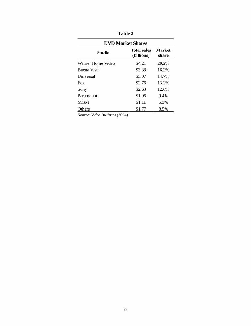
27

Table 3

DVD Market Shares

Studio Total sales (billions)

Market share

Warner Home Video $4.21 20.2% Buena Vista $3.38 16.2% Universal $3.07 14.7% Fox $2.76 13.2% Sony $2.63 12.6% Paramount $1.96 9.4% MGM $1.11 5.3% Others $1.77 8.5% Source: Video Business (2004)

28

Table 4

Consumer Survey Data: Descriptive Statistics Variable Category Mean

(1) Preference for movie-going "Like Very Much" 0.30 "Like Somewhat" 0.41 "Don’t Like it Very Much" 0.14 "Do Not Do It At All" 0.15 (2) Preference for video-watching "Like Very Much" 0.38 "Like Somewhat" 0.43 "Don’t Like it Very Much" 0.09 "Do Not Do It At All" 0.10 Polychoric correlation coefficient b/w (1) and (2)a 0.45 Favorite movie genres Action/Adventure 0.60 Animated 0.18 Comedy 0.68 Drama 0.49 Horror/Suspense 0.28 Musical 0.20 Romance 0.31 Science Fiction 0.28 Foreign 0.06 Importance for choose movies Stars/director 2.00 Advertising 1.92 Critic Review 1.61 WOM 2.33 Awards/Nominations 1.58 Importance for choose videos Stars/director 2.06 Advertising 1.77 WOM 2.26 Awards/Nominations 1.54 Likelihood of repeat watching "Rarely" 0.33 "Sometimes" 0.45 "Frequently" 0.22 a The Pearson correlation coefficient is 0.40.

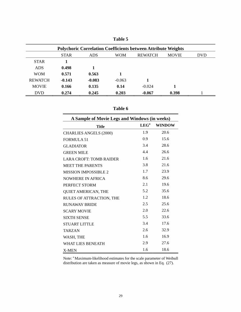
29

Table 5

Polychoric Correlation Coefficients between Attribute Weights STAR ADS WOM REWATCH MOVIE DVD

STAR 1 ADS 0.498 1

WOM 0.571 0.563 1 REWATCH -0.143 -0.083 -0.063 1

MOVIE 0.166 0.135 0.14 -0.024 1 DVD 0.274 0.245 0.203 -0.067 0.398 1

Table 6

A Sample of Movie Legs and Windows (in weeks)

Title LEGa WINDOW

CHARLIES ANGELS (2000) 1.9 20.6 FORMULA 51 0.9 15.6 GLADIATOR 3.4 28.6 GREEN MILE 4.4 26.6 LARA CROFT: TOMB RAIDER 1.6 21.6 MEET THE PARENTS 3.8 21.6 MISSION IMPOSSIBLE 2 1.7 23.9 NOWHERE IN AFRICA 8.6 29.6 PERFECT STORM 2.1 19.6 QUIET AMERICAN, THE 5.2 35.6 RULES OF ATTRACTION, THE 1.2 18.6 RUNAWAY BRIDE 2.5 25.6 SCARY MOVIE 2.0 22.6 SIXTH SENSE 5.5 33.6 STUART LITTLE 3.4 17.6 TARZAN 2.6 32.9 WASH, THE 1.6 16.9 WHAT LIES BENEATH 2.9 27.6 X-MEN 1.6 18.6

Note: a Maximum-likelihood estimates for the scale parameter of Weibull distribution are taken as measure of movie legs, as shown in Eq. (27).

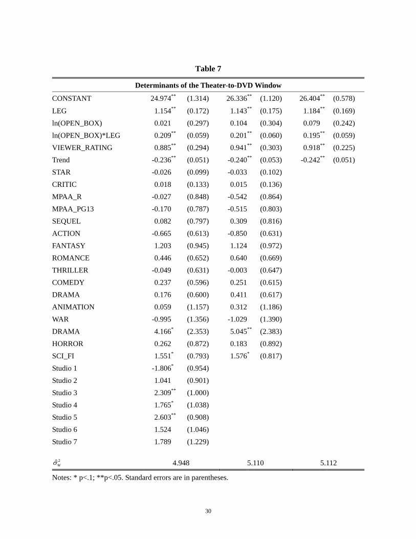
30

Table 7

Determinants of the Theater-to-DVD Window

CONSTANT 24.974 ** (1.314) 26.336 ** (1.120) 26.404 ** (0.578)

LEG 1.154 ** (0.172) 1.143 ** (0.175) 1.184 ** (0.169) ln(OPEN_BOX) 0.021 (0.297) 0.104 (0.304) 0.079 (0.242) ln(OPEN_BOX)*LEG 0.209 ** (0.059) 0.201 ** (0.060) 0.195 ** (0.059) VIEWER_RATING 0.885 ** (0.294) 0.941 ** (0.303) 0.918 ** (0.225) Trend -0.236 ** (0.051) -0.240 ** (0.053) -0.242 ** (0.051) STAR -0.026 (0.099) -0.033 (0.102) CRITIC 0.018 (0.133) 0.015 (0.136) MPAA_R -0.027 (0.848) -0.542 (0.864) MPAA_PG13 -0.170 (0.787) -0.515 (0.803) SEQUEL 0.082 (0.797) 0.309 (0.816) ACTION -0.665 (0.613) -0.850 (0.631) FANTASY 1.203 (0.945) 1.124 (0.972) ROMANCE 0.446 (0.652) 0.640 (0.669) THRILLER -0.049 (0.631) -0.003 (0.647) COMEDY 0.237 (0.596) 0.251 (0.615) DRAMA 0.176 (0.600) 0.411 (0.617) ANIMATION 0.059 (1.157) 0.312 (1.186) WAR -0.995 (1.356) -1.029 (1.390) DRAMA 4.166 * (2.353) 5.045 ** (2.383) HORROR 0.262 (0.872) 0.183 (0.892) SCI_FI 1.551 * (0.793) 1.576 * (0.817) Studio 1 -1.806 * (0.954) Studio 2 1.041 (0.901) Studio 3 2.309 ** (1.000) Studio 4 1.765 * (1.038) Studio 5 2.603 ** (0.908) Studio 6 1.524 (1.046) Studio 7 1.789 (1.229)

2ˆWσ 4.948 5.110 5.112

Notes: * p<.1; **p<.05. Standard errors are in parentheses.

31

Table 8

Determinants of DVD Pricea

Constant 3.088 ** (0.017)

ln(OPEN_BOX) -0.011 ** (0.004)

STAR 0.001 (0.002)

CRITIC 0.000 (0.002)

VIEWER_RATING 0.005 (0.004)

MPAA_R 0.004 (0.014)

MPAA_PG13 -0.003 (0.013)

SEQUEL 0.012 (0.013)

ACTION -0.021 ** (0.010)

FANTASY -0.011 (0.015)

ROMANCE 0.003 (0.011)

THRILLER -0.017 (0.010)

COMEDY 0.001 (0.010)

DRAMA 0.004 (0.010)

ANIMATION -0.001 (0.019)

WAR -0.017 (0.022)

DRAMA -0.045 (0.038)

HORROR 0.005 (0.014)

SCI_FI -0.008 (0.013)

Trend -0.010 ** (0.001)

Pσ 0.081 ** (0.021) Notes: Dependent variable is the logarithm of DVDretail price. * p<.1; **p<.05. Standard errors are in parentheses.

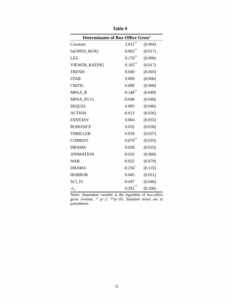
32

Table 9

Determinants of Box-Office Grossa Constant 3.612 ** (0.064)

ln(OPEN_BOX) 0.902 ** (0.017) LEG 0.176 ** (0.006) VIEWER_RATING 0.105 ** (0.017) TREND 0.000 (0.003) STAR 0.009 (0.006) CRITIC 0.000 (0.008) MPAA_R -0.148 ** (0.049) MPAA_PG13 -0.048 (0.046) SEQUEL 0.005 (0.046) ACTION -0.013 (0.036) FANTASY 0.004 (0.055) ROMANCE 0.032 (0.038) THRILLER 0.018 (0.037) COMEDY 0.079 ** (0.035) DRAMA 0.028 (0.035) ANIMATION -0.033 (0.068) WAR -0.022 (0.079) DRAMA -0.256 * (0.135) HORROR 0.043 (0.051) SCI_FI -0.047 (0.046)

Bσ 0.291 ** (0.106)

Notes: Dependent variable is the logarithm of box-office gross revenue. * p<.1; **p<.05. Standard errors are in parentheses.

33

Table 10

Theatrical-Movie Utility Parameters CONSTANT -13.256 ** (0.141) ln(AD_SPEND) 0.248 ** (0.034) STAR 0.080 ** (0.008) CRITIC -0.017 * (0.010) VIEWER_RATING 0.042 ** (0.020) R -0.101 * (0.061) PG13 -0.021 (0.056) SEQUEL -0.084 (0.052) ACTION -0.073 (0.046) FANTASY -0.097 (0.059) ROMANCE -0.173 ** (0.048) TRILLER 0.132 ** (0.046) COMEDY 0.215 ** (0.042) DRAMA 0.048 (0.043) ANIMATION 0.114 (0.076) WAR -0.122 (0.103) DOCUMENTARY -0.235 (0.197) HORROR 0.125 ** (0.061) SCI-FI 0.050 (0.056) SPRING 0.251 ** (0.055) SUMMER 0.179 ** (0.049) FALL 0.101 * (0.052) HOLIDAY 0.236 ** (0.059) ln(SCREENS) 1.124 ** (0.015) DECAY_RATE -0.438 ** (0.008)

Heterogeneity dispersion

CONSTANT 0.177 (0.141) STAR 0.115 ** (0.017)

DECAY_RATE 0.265 ** (0.011)

34

Table 11

DVD Utility Parameters Rental Collection CONSTANT -0.972** (0.400) 1.931 ** (0.834) ln(Box Office Revenue) 0.624** (0.016) 1.106 ** (0.020) WINDOW -0.075** (0.029) -0.061 ** (0.012) STAR 0.031** (0.005) -0.010 (0.006) CRITIC -0.015** (0.007) -0.015 * (0.008) VIEWER_RATING -0.015 (0.019) -0.043 ** (0.017) MPAA_R 0.577** (0.046) 0.171 ** (0.049) MPAA_PG13 0.466** (0.043) -0.110 ** (0.044) SEQUEL -0.356** (0.042) -0.143 ** (0.044) ACTION -0.066** (0.027) 0.172 ** (0.033) FANTASY 0.080* (0.048) 0.271 ** (0.055) ROMANCE -0.091** (0.038) -0.187 ** (0.041) THRILLER 0.199** (0.030) 0.084 ** (0.040) COMEDY 0.026 (0.030) -0.103 ** (0.038) DRAMA -0.027 (0.027) -0.024 (0.033) ANIMATION -0.638** (0.121) 0.012 (0.105) WAR 0.153** (0.062) 0.235 ** (0.063) DRAMA -0.436** (0.120) -0.160 ** (0.071) HORROR 0.013 (0.038) 0.057 (0.051) SCI_FI 0.037 (0.037) 0.009 (0.047) COMMENTARY 0.038 (0.028) 0.092 ** (0.033) DEL_SCENES 0.071** (0.023) 0.066 ** (0.027) MUSIC -0.102** (0.028) 0.172 ** (0.030) GAMES 0.209 (0.136) 0.300 ** (0.131) Trend -0.257** (0.010) -0.524 ** (0.015)

ln(PRICE) -2.302** (0.288)

0d -0.022* (0.013)

0c 0.151** (0.07)

35

Table 12

Dynamic Linkage Parameters

Substitutability parameters (SE)

Constant 0.153 ** (0.213)

Viewer Rating -0.120 ** (0.034)

Animation -0.312 ** (0.135)

R-Rated 0.110 * (0.065)2gσ 0.113 ** (0.050)

Forward-looking parameter

λ -5.739 ** (1.985)

Table 13

Simulated Effects of Window Reduction

Reduction in the Average

Window (Weeks)

Change in theater

admission per movie (000)

Change in DVD Sales

Change in DVD Rentals

Industry Revenue

0 0.00 0.00 0.00 0.00 3 -35.82 45.80 32.50 42.48 6 -79.21 88.50 68.30 77.59 9 -133.83 133.50 99.21 98.88

12 -206.75 190.55 122.10 105.90 15 -310.28 240.30 159.39 89.41 18 -380.40 261.90 170.20 51.70

Table 14

Windowing Schedule of a Typical Movie Version Release Time

Theatrical Exhibition Initial debut Home Video 5 months later

Pay-Per-View (or Video-on-Demand) 8 months later Pay-TV (e.g., HBO) 12 months later Network/Syndication 2-3 years later

36

Figures

Figure 1

DVD Hardware Installation Base in the U.S.

0

10

20

30

40

50

60

70

Jan-00 Jan-01 Jan-02 Jan-03 Jan-04

Num

ber

of h

ouse

hold

s (m

ils.)

Figure 2

Histogram: Theatar-to-DVD windows

0

20

40

60

80

100

120

140

160

60 100 140 180 220 260 300 340Days

Num

ber

of m

ovie

s

The sample consists of DVDs of feature movies released between Jan. 2000 and Oct. 2003. (N=526)

37

Figure 3: Weibull Fitting of Box-Office Sales

The Sixth Sense

0

10

20

30

40

50

1 2 3 4 5 6 7 8 9

Week

Rev

enue

($ M

ils.)

FittedActual

Nowhere in Africa

00.10.20.30.40.50.60.70.8

1 2 3 4 5 6 7 8 9

Week

Rev

enue

($ M

ils.)

FittedActual

Bend It Like Beckham

0

0.5

1

1.5

2

2.5

3

1 2 3 4 5 6 7 8 9

Week

Rev

enue

($ M

ils.)

FittedActual

The Importance of Being Earnest

0

0.5

1

1.5

2

1 2 3 4 5 6 7 8 9

Week

Rev

enue

($ M

ils.)

FittedActual

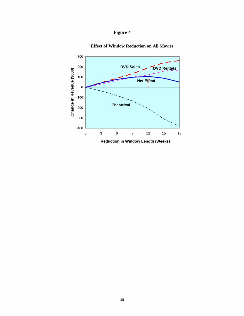
38

Figure 4

Effect of Window Reduction on All Movies

-400

-300

-200

-100

0

100

200

300

0 3 6 9 12 15 18

Reduction in Window Length (Weeks)

Cha

nge

in R

even

ue ($

000)

Theatrical

DVD Sales DVD Rentals

Net Effect