Optimal Forest Strategies for Addressing Tradeoffs and Uncertainty in Economic Development under Old-Growth Constraints

by

Emina Krcmar†, Alison J. Eagle‡ and G. Cornelis van Kooten‡*

† FEPA Research Unit, University of British Columbia

‡Department of Economics, University of Victoria

*Corresponding Author: P.O. Box 1700, Stn CSC, Victoria, BC, Canada V8W 2Y2 ph: 250-721-8539; e-mail: kooten@uvic.ca

Selected paper prepared for presentation at the joint Canadian Agricultural Economics Society and American Agricultural Economics Association Annual Meeting, Portland,

OR, July 29 – August 1, 2007 Copyright 2007 by E. Krcmar, A.J. Eagle and G.C. van Kooten. All rights reserved. Readers may make verbatim copies of this document for non-commercial purposes by any means, provided that this copyright notice appears on all such copies.

Abstract

In Canada, governments have historically promoted economic development in rural

regions by promoting exploitation of natural resources, particularly forests. Forest resources

are an economic development driver in many of the more than 80% of native communities

located in forest regions. But forests also provide aboriginal people with cultural and spiritual

values, and non-timber forest amenities (e.g., biodiversity, wildlife harvests for meat and fur,

etc.), that are incompatible with timber exploitation. Some cultural and other amenities can

only be satisfied by maintaining a certain amount of timber in an old-growth state. In that

case, resource constraints might be too onerous to satisfy development needs. We employ

compromise programming and fuzzy programming to identify forest management strategies

that best compromise between development and other objectives, applying our models to an

aboriginal community in northern Alberta. In addition to describing how mathematical

programming techniques can be applied to regional development and forest management, we

conclude from the analysis that no management strategy is able to satisfy all of the technical,

environmental and social/cultural constraints and, at the same time, offer aboriginal peoples

forest-based economic development. Nonetheless, we demonstrate that extant forest

management policies can be improved upon.

Keywords: forest-dependent aboriginal communities; boreal forest; compromise and

fuzzy programming; sustainability and uncertainty

JEL Categories: R11, Q23, Q01, C61

ii

Optimal Forest Strategies for Addressing Tradeoffs and Uncertainty in Economic Development under Old-Growth Constraints

Introduction

Alberta forest policy requires sustained yield management, which is implemented using

harvest levels and growth rates as indicators. The sustained yield policy requires that harvest

levels not exceed average timber growth (annual harvests equal mean annual increment); but it

also implies maximizing cumulative harvest volume (because it is related to total employment),

while maintaining an even flow of harvests (in order to maintain employment and regional

economic stability) over some planning horizon. While this might be considered a decent rule of

thumb, the five-year planning period militates against this practical approach to sustainability,

partly because the planning period does not coincide with the forest rotation age and fails to take

into account longer term factors affecting forest dynamics. The sustained yield policy flies in the

face of uncertainty regarding growth and yield, natural disturbances (fire, disease and insect

infestations), price volatility, climate change, and even shifts in forest policies themselves.

In Canada, many aboriginal people live in forest-dependent communities. They are

subject to provincial forest policies that are short-sighted to say the least. Yet, the well being of

aboriginal people spans a much longer period of time than that considered in forest management

plans. In this paper, we focus on the consequences of this for the Little Red River Cree Nation

(LRRCN) of northern Alberta, a forest-dependent community seeking to use forest resources as a

springboard for economic development. We assume that the goal of the LRRCN is to develop

and implement a forest management strategy that will ensure the community’s economic

sustainability, while preserving a forest landscape with features critical to cultural values and on-

going traditional use of the forest. In this regard, preservation of old-growth forest is integral to

First Nations’ beliefs: “The value First Nations people place on old-growth forests often reflects

the fact that old growth is crucial to their continued existence. Old growth is inextricably bound

to the culture of First Nations and this fact has to be recognized in management decisions, as

there is simply no replacement for old growth forest for many aspects of First Nations culture”

(Walkem 1994, p.3). But maintaining old growth is also a special consideration of management

because of its contribution to biodiversity (Spies and Franklin 1996; Burton et al. 1999).

Aboriginal peoples have historically occupied portions of the Lower Peace River region

in north-central Alberta and used these lands to support their culture and livelihood. Treaty No. 8

(1899) affirmed their right to use the resources within their historical area; the forest resources

were legally meant to sustain traditional vocations and way-of-life. As part of this mandate,

LRRCN was able to form its own forest management company, Little Red River Forestry

(LRRF), and a company holding timber quota that can be sold to forest companies (Askee

Development Corporation). In 1995, the LRRCN and the neighboring Tall Cree First Nation

entered into a cooperative management planning agreement with the Alberta Government and

Tolko Industries Ltd. (MOU 1996). In addition to the agreements with Tolko, a volume

agreement was later signed between LRRCN and Footner Forest Products Ltd. (MOU 1999) to

supply deciduous fiber to an oriented strand board (OSB) mill. Under these agreements, the

companies compensate LRRF for the costs of harvesting and reforestation (although only

coniferous stands are replanted as deciduous stands are left to regenerate naturally). As the quota

holder for LRRCN, Askee Development Corporation also receives stumpage fees for harvested

timber, with payments linked to product prices in a manner similar to that used by the Alberta

Government to establish stumpage rates. However, the Alberta Government also collects

2

stumpage on volumes harvested under these tenures so aboriginal people do not collect all of the

resource rent.

Arguably, the federal and provincial governments may not lived up to the Treaty 8

obligations, as aboriginal people do not have access to the timber resources on all Treaty 8 lands.

Rather, they are relegated to Forest Management Unit F23 (see Figure 1) and some other smaller

parcels. Are these adequate to support the aboriginal community, as seems to be required under

the Treaty? To examine the resource constraints facing LRRCN, we focus on management unit

F23, for which comprehensive timber resource information is available. Other timber resources

in the region are ignored as these are generally spoken for and would not significantly change the

analysis in this paper.

The current strategy employed by LRRF to manage F23 was designed to satisfy the co-

management agreements between LRRCN, the forest industry and government (MOU 1996,

1999). In this study, we take the aboriginal objectives to be economic development, community

stability and employment, although we recognize that these goals are not mutually exclusive.

Community stability is represented by even-flow timber supply and little downside variation in

employment, while economic development is based on net returns from timber and silvicultural

operations. Employment opportunities are found primarily in logging and silviculture, but these

could be short term (allocating harvest towards the present) or long term.

To address the potential for economic development in a forest dependent community, we

apply methods of multiple-objective decision-making using compromise and fuzzy programming

methods. Following Krcmar and van Kooten (2007), we employ two outcomes from compromise

programming to construct membership functions to be used in fuzzy programming. This avoids

the need to solicit preference information from decision makers. The current research differs

3

from the previous study in our focus on ecological outcomes as represented by the retention of

old-growth forests, which are important to aboriginal people (as noted above). We begin in the

next section with a formal description of the problem and the mathematical programming models

that we use to answer policy questions concerning appropriate development strategies. This is

followed by a more detailed discussion of compromise and fuzzy programming, and a section

that presents the objective values under various forest management strategies. In essence, these

determine the optimal tradeoffs available, with the fuzzy programming model in essence

choosing the best compromise that is available. We then examine how employment and forest

structure change over time under various management options. Some concluding observations

complete the discussion.

Problem Description and Model Formulation

To address the economic, employment and timber supply objectives, we require

indicators that provide objective measures for determining the extent to which objectives are

satisfied. Thus, the economic measure consists of the net discounted returns to logging and

timberland management more generally. For employment, we use both long- and short-term jobs

in logging and silviculture (as natives are not currently employed in manufacturing). Long-term

employment is measured as the cumulative employment over the entire planning horizon, while

the short-term measure constitutes total employment over early periods only. Short-term

employment will inevitably take precedence over long-term employment, although the latter

better indicates the ability of a small community to survive on the timber resource base,

assuming that non-forest related economic opportunities gravitate to larger centers.

The timber supply objective addresses concerns relate to providing adequate fiber for

mills and satisfying contractual obligations with the Province and industry. This objective is

4

typically accomplished through even-flow harvest over time. We couple even-flow harvest to the

objective of maximizing cumulative harvest volume over the planning horizon, because this

drives fiber supply as high as possible (thereby also enhancing employment in logging).

To examine the ability of local timber resources to support a sustainable economic base

and perhaps economic development in forest-dependent native communities, we construct

several strategic forest planning models. We used a 200-year planning horizon (2005 to 2205)

divided into twenty decades, chosen according to the strategic planning practices in Canada.

Specifically, we formulate models to determine harvest schedules that seek to achieve:

1. An economic objective of maximizing the cumulative discounted net returns from forestry;

2. Long- and short-term social objectives expressed as maximizing potential cumulative

employment in forest operations over the (a) entire planning horizon and (b) first several

periods;

3. Timber supply objectives that are formulated in terms of maximizing cumulative harvest

volume over the planning horizon and minimizing maximum deviation of softwood and

hardwood harvest flow; and

4. Ecological objectives expressed as preserving a certain amount of old growth over the whole

planning horizon.

The harvest flow requirements address concerns related to adequate timber supply for

mills, and thereby jobs and community stability. The output generated by employment in various

forest activities is provided in Table 1. This relation between activities and jobs is assumed to

remain unchanged over the planning horizon, which implies that we err on the side of higher

employment as technological change will undoubtedly impact the relationships in Table 1.

5

There are two general approaches for defining targets on preservation of old-growth

forests: One is to calculate the expected proportion of old growth based on the annual incidence

of natural disturbance, especially fire; the other is to utilize the pattern present in the existing

forest. We define old-growth targets using the latter approach. The extant proportions of old

coniferous and deciduous forests in the study region are 34.6% and 6.8%, respectively, where old

growth is defined as forests older than 100 years. Based on the initial inventory patterns and

expected near-future regulations, we set the targets for preserving old coniferous and deciduous

forests at 18% and 6% of their respective harvest areas. The timber management area comprises

42.5% of coniferous forest and 57.5% of deciduous forest. So an old growth target of 11.1% is

calculated as a weighted average of the 18% and 6% targets for old coniferous and deciduous

growth.

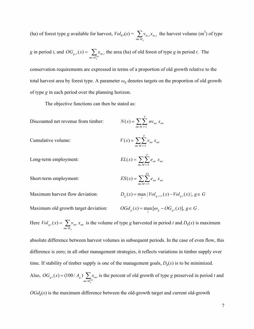
Harvest scheduling decisions are addressed in a non-spatial manner using model elements

defined as follows. Forest attributes are aggregated into management strata, where a stratum m is

defined by a combination of tree species, density, height and age. Let M denote the set of

management strata, T the number of planning periods, TS <T the number of periods considered

for short-term employment, and },{, decidconifGgMM g =∈⊂ a partition of M by the

coniferous and deciduous forest types g. We also introduce a set that contains old

growth strata of type g. The index sets, and , allow us to address constraints and

objectives specific to coniferous and deciduous old-growth forest types.

MM OGg ⊂

gM OGgM

A decision variable x = xmt represents a forest management strategy expressed as the area

(in ha) of stratum m harvested in period t. Denote the merchantable volume from a ha of stratum

m harvested in period t by vmt, the net discounted revenue per ha of stratum m in period t by nvmt,

and employment generated by harvesting a ha of stratum m in period t by emt. Let Ag be the area

6

(ha) of forest type g available for harvest, Volg,t(x) = tmMm

tm xvg

,,∑∈

the harvest volume (m3) of type

g in period t, and the area (ha) of old forest of type g in period t. The

conservation requirements are expressed in terms of a proportion of old growth relative to the

total harvest area by forest type. A parameter ωg denotes targets on the proportion of old growth

of type g in each period over the planning horizon.

∑∈

=OGgMm

tmtg xxOG ,, )(

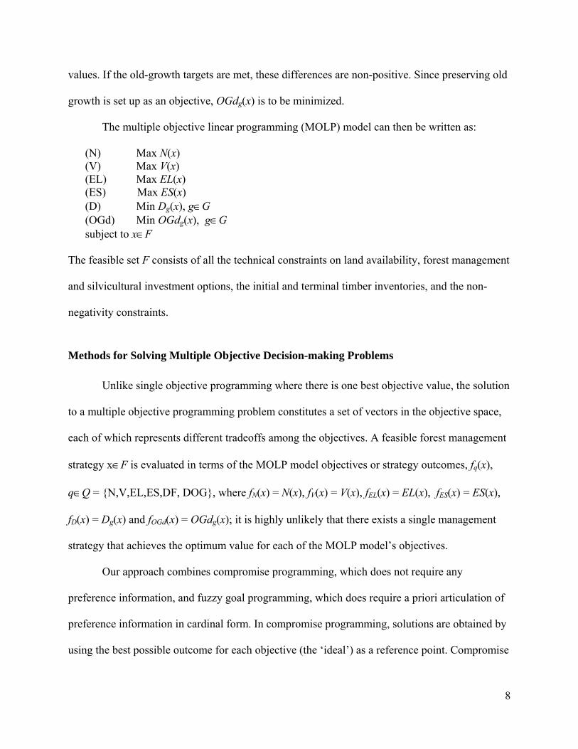
The objective functions can then be stated as:

Discounted net revenue from timber: mtmtMm

T

txnvxN ∑∑

∈ =

=1

)(

Cumulative volume: mtMm

T

tmt xvxV ∑∑

∈ =

=1

)(

Long-term employment: mtMm

T

tmt xexEL ∑∑

∈ =

=1

)(

Short-term employment: mtMm

TS

tmt xexES ∑∑

∈ =

=1

)(

Maximum harvest flow deviation: GgxVolxVolxD tgtgtg ∈−= + |,)()(|max)( 1,

Maximum old growth target deviation: GgxOGxOGd tggtg ∈−= )],([max)( ω .

Here is the volume of type g harvested in period t and Dg(x) is maximum

absolute difference between harvest volumes in subsequent periods. In the case of even flow, this

difference is zero; in all other management strategies, it reflects variations in timber supply over

time. If stability of timber supply is one of the management goals, Dg(x) is to be minimized.

Also, is the percent of old growth of type g preserved in period t and

OGdg(x) is the maximum difference between the old-growth target and current old-growth

mtMm

mttg xvxVolg

∑∈

=)(

∑∈

=OGgMm

tmgtg xAxOG )/100()(

7

values. If the old-growth targets are met, these differences are non-positive. Since preserving old

growth is set up as an objective, OGdg(x) is to be minimized.

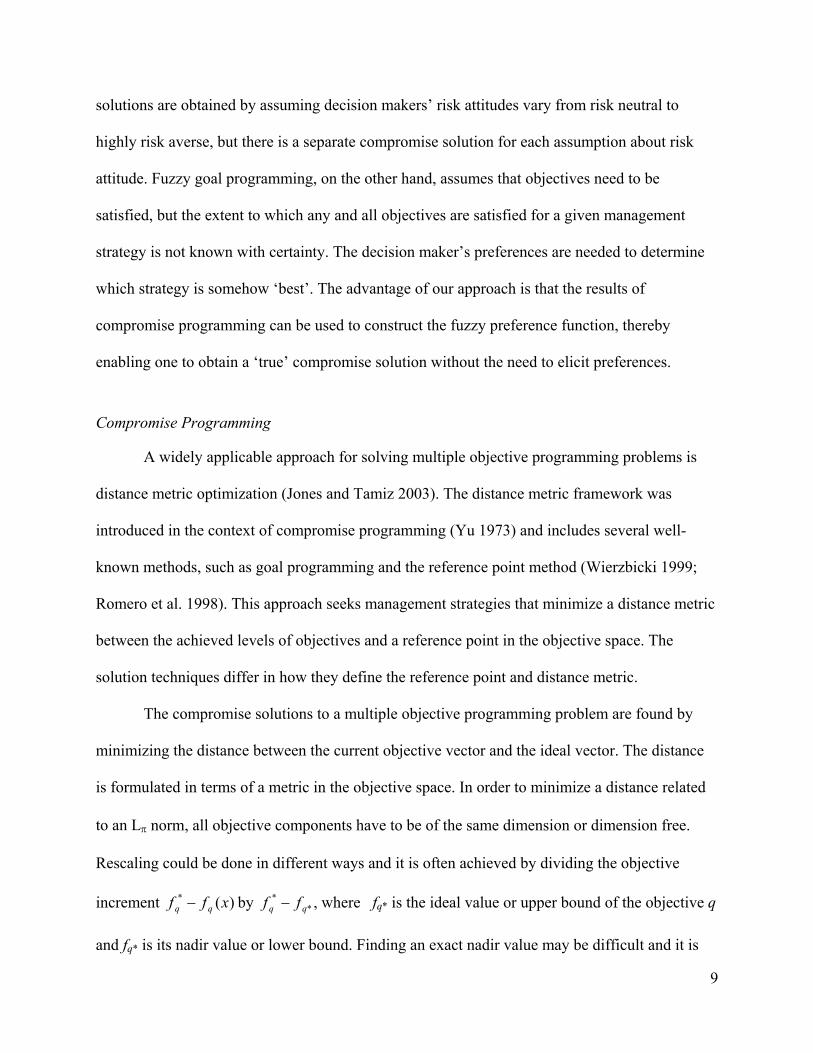
The multiple objective linear programming (MOLP) model can then be written as:

(N) Max N(x) (V) Max V(x) (EL) Max EL(x) (ES) Max ES(x) (D) Min Dg(x), g∈G

(OGd) Min OGdg(x), g∈G subject to x∈F

The feasible set F consists of all the technical constraints on land availability, forest management

and silvicultural investment options, the initial and terminal timber inventories, and the non-

negativity constraints.

Methods for Solving Multiple Objective Decision-making Problems

Unlike single objective programming where there is one best objective value, the solution

to a multiple objective programming problem constitutes a set of vectors in the objective space,

each of which represents different tradeoffs among the objectives. A feasible forest management

strategy x∈F is evaluated in terms of the MOLP model objectives or strategy outcomes, fq(x),

q∈Q = {N,V,EL,ES,DF, DOG}, where fN(x) = N(x), fV(x) = V(x), fEL(x) = EL(x), fES(x) = ES(x),

fD(x) = Dg(x) and fOGd(x) = OGdg(x); it is highly unlikely that there exists a single management

strategy that achieves the optimum value for each of the MOLP model’s objectives.

Our approach combines compromise programming, which does not require any

preference information, and fuzzy goal programming, which does require a priori articulation of

preference information in cardinal form. In compromise programming, solutions are obtained by

using the best possible outcome for each objective (the ‘ideal’) as a reference point. Compromise

8

solutions are obtained by assuming decision makers’ risk attitudes vary from risk neutral to

highly risk averse, but there is a separate compromise solution for each assumption about risk

attitude. Fuzzy goal programming, on the other hand, assumes that objectives need to be

satisfied, but the extent to which any and all objectives are satisfied for a given management

strategy is not known with certainty. The decision maker’s preferences are needed to determine

which strategy is somehow ‘best’. The advantage of our approach is that the results of

compromise programming can be used to construct the fuzzy preference function, thereby

enabling one to obtain a ‘true’ compromise solution without the need to elicit preferences.

Compromise Programming

A widely applicable approach for solving multiple objective programming problems is

distance metric optimization (Jones and Tamiz 2003). The distance metric framework was

introduced in the context of compromise programming (Yu 1973) and includes several well-

known methods, such as goal programming and the reference point method (Wierzbicki 1999;

Romero et al. 1998). This approach seeks management strategies that minimize a distance metric

between the achieved levels of objectives and a reference point in the objective space. The

solution techniques differ in how they define the reference point and distance metric.

The compromise solutions to a multiple objective programming problem are found by

minimizing the distance between the current objective vector and the ideal vector. The distance

is formulated in terms of a metric in the objective space. In order to minimize a distance related

to an Lπ norm, all objective components have to be of the same dimension or dimension free.

Rescaling could be done in different ways and it is often achieved by dividing the objective

increment by , where fq* is the ideal value or upper bound of the objective q

and fq* is its nadir value or lower bound. Finding an exact nadir value may be difficult and it is

)(* xff qq − **

qq ff −

9

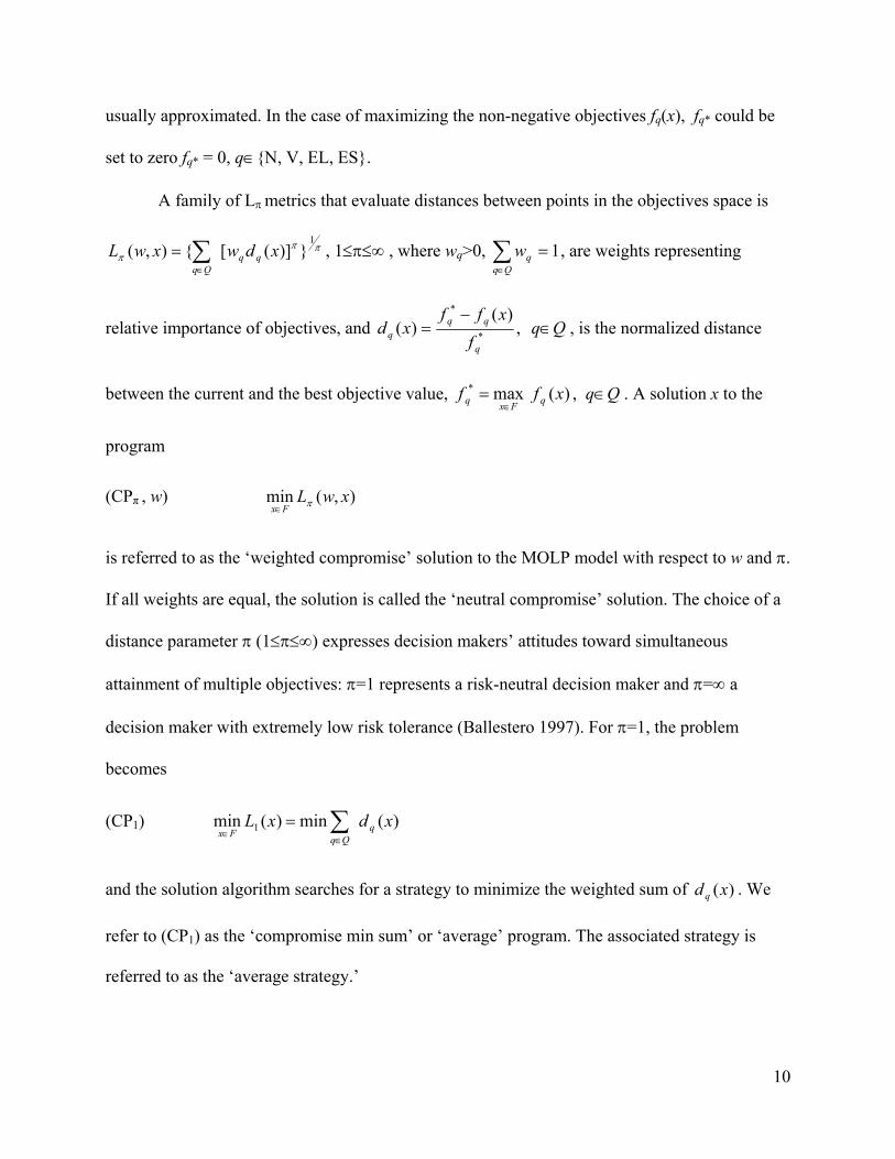
usually approximated. In the case of maximizing the non-negative objectives fq(x), fq* could be

set to zero fq* = 0, q∈{N, V, EL, ES}.

A family of Lπ metrics that evaluate distances between points in the objectives space is

πππ

1})]([{),( xdwxwL qq

Qq∑∈

= , 1≤π≤∞ , where wq>0, 1=∑∈Qq

qw , are weights representing

relative importance of objectives, and ,)(

)( *

*

q

qqq f

xffxd

−= q∈Q , is the normalized distance

between the current and the best objective value, , q∈Q . A solution x to the

program

)(max* xff qFxq ∈=

(CPπ , w) ),(min xwLFx π∈

is referred to as the ‘weighted compromise’ solution to the MOLP model with respect to w and π.

If all weights are equal, the solution is called the ‘neutral compromise’ solution. The choice of a

distance parameter π (1≤π≤∞) expresses decision makers’ attitudes toward simultaneous

attainment of multiple objectives: π=1 represents a risk-neutral decision maker and π=∞ a

decision maker with extremely low risk tolerance (Ballestero 1997). For π=1, the problem

becomes

(CP1) )(min)(min 1 xdxL qQqFx ∑

∈∈

=

and the solution algorithm searches for a strategy to minimize the weighted sum of . We

refer to (CP1) as the ‘compromise min sum’ or ‘average’ program. The associated strategy is

referred to as the ‘average strategy.’

)(xd q

10

As π increases, more weight is put on the largest dq(x). Ultimately, the largest distance

completely dominates and, for π=∞, becomes:

(CP∞) . )(maxmin)(min xdxL qQqFxFx ∈∈∞∈=

If )(max xdqQq∈=λ , then the program (CP∞) could be rewritten as:

min λ

(CP∞) subject to

Fx

Qqf

xffxd

q

qqq

∈

∈≤−

= ,)(

)( *

*

λ

The solution in this case balances all objectives in terms of their normalized distances from the

best values. We refer to (CP∞) as the ‘compromise min max’ or ‘balanced’ program, with an

associated strategy called a ‘balanced strategy.’

The metric Lπ has an important practical feature for both π=1 and π=∞, namely, that the

model’s linearity is preserved. This is important given the size and complexity of the

programming model. However, the linearity assumption is not restricting because solutions for

(CPπ) (1<π<∞) lie between the solutions for (CP1) and (CP∞).

The solutions of the compromise program (CPπ) are affected not only by the choice of

parameter π, but also by the normalization method used for distance calculation. Solutions of

(CPπ) with equal weighting coefficients are neutral compromise strategies with the

corresponding outcomes located somewhere in the middle of the Pareto-optimal frontier. These

solutions serve only to eliminate obviously bad strategies and are typically used as a starting

point in a search for an acceptable solution.

11

Fuzzy Programming

In compromise programming, the application of the ideal as a reference point avoids

having to determine the decision maker’s preferences, thus providing objectivity to the solution

process. The drawback is that it likely result in outcomes far from the desired targets. Different

approaches have been suggested to fix this problem. The most widely used multiple objective

decision making technique is goal programming, which requires information about desired

objective targets. The preferred solution is defined as the one that minimizes a combined

deviation from the set of targets. A difficulty with defining the targets is that they are not known

exactly. In addition to this vagueness of the targets originating in the decision maker’s

preferences, there is an uncertainty resulting from environmental, economic and social

conditions. Factors that may affect the targets include: (i) growth and yield as a function of

weather, climate change and soil conditions; (ii) natural disturbances; (iii) forest policy changes

(e.g., a shift from sustained yield to sustainable forest management); (iv) market conditions in

the form of demand for forest products and likely fluctuating prices; (v) distribution between

softwood and hardwood harvest and subsequent consequences for employment in silviculture

and logging; and (vi) technological changes over the short and long terms. Not all of these

factors affect each of the objective values and targets, but several of them contribute to

imprecision of outcomes and goals.

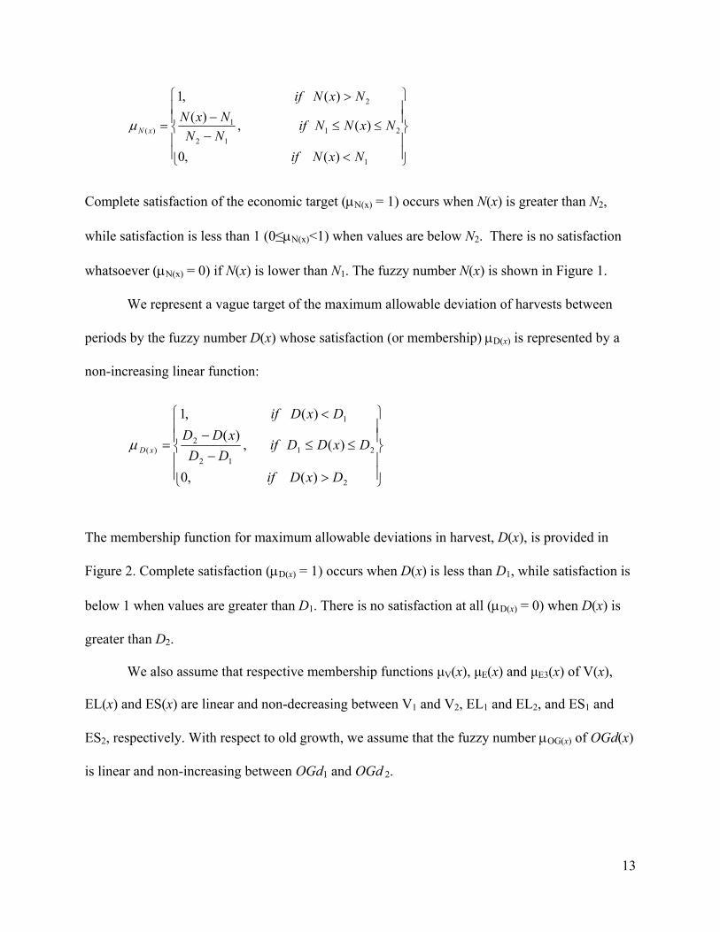
In this paper, the vague targets are quantified using fuzzy numbers. A vague financial

target related to timber benefits can be represented by the fuzzy number N(x) whose satisfaction,

or membership μN(x), is represented by a non-decreasing linear function:

12

⎪⎪⎭

⎪⎪⎬

⎫

⎪⎪⎩

⎪⎪⎨

⎧

<

≤≤−−

>

=

1

2112

1

2

)(

)(,0

)(,)()(,1

NxNif

NxNNifNNNxN

NxNif

xNμ

Complete satisfaction of the economic target (μN(x) = 1) occurs when N(x) is greater than N2,

while satisfaction is less than 1 (0≤μN(x)<1) when values are below N2. There is no satisfaction

whatsoever (μN(x) = 0) if N(x) is lower than N1. The fuzzy number N(x) is shown in Figure 1.

We represent a vague target of the maximum allowable deviation of harvests between

periods by the fuzzy number D(x) whose satisfaction (or membership) μD(x) is represented by a

non-increasing linear function:

⎪⎪⎭

⎪⎪⎬

⎫

⎪⎪⎩

⎪⎪⎨

⎧

>

≤≤−−

<

=

2

2112

2

1

)(

)(,0

)(,)(

)(,1

DxDif

DxDDifDD

xDDDxDif

xDμ

The membership function for maximum allowable deviations in harvest, D(x), is provided in

Figure 2. Complete satisfaction (μD(x) = 1) occurs when D(x) is less than D1, while satisfaction is

below 1 when values are greater than D1. There is no satisfaction at all (μD(x) = 0) when D(x) is

greater than D2.

We also assume that respective membership functions μV(x), μE(x) and μE3(x) of V(x),

EL(x) and ES(x) are linear and non-decreasing between V1 and V2, EL1 and EL2, and ES1 and

ES2, respectively. With respect to old growth, we assume that the fuzzy number μOG(x) of OGd(x)

is linear and non-increasing between OGd1 and OGd 2.

13

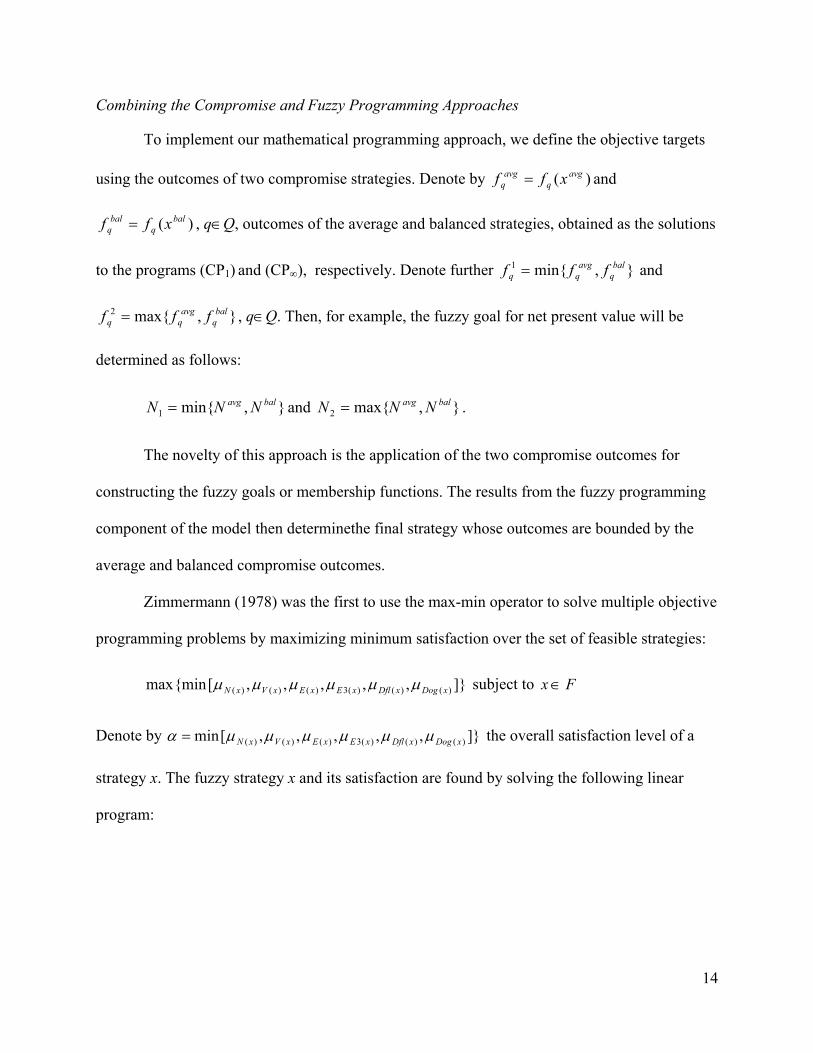
Combining the Compromise and Fuzzy Programming Approaches

To implement our mathematical programming approach, we define the objective targets

using the outcomes of two compromise strategies. Denote by and

, q∈Q, outcomes of the average and balanced strategies, obtained as the solutions

to the programs (CP1) and (CP∞), respectively. Denote further and

, q∈Q. Then, for example, the fuzzy goal for net present value will be

determined as follows:

)( avgq

avgq xff =

)( balq

balq xff =

},min{1 balq

avgqq fff =

},max{2 balq

avgqq fff =

},min{1balavg NNN = and . },max{2

balavg NNN =

The novelty of this approach is the application of the two compromise outcomes for

constructing the fuzzy goals or membership functions. The results from the fuzzy programming

component of the model then determinethe final strategy whose outcomes are bounded by the

average and balanced compromise outcomes.

Zimmermann (1978) was the first to use the max-min operator to solve multiple objective

programming problems by maximizing minimum satisfaction over the set of feasible strategies:

]},,,,,[{minmax )()()(3)()()( xDogxDflxExExVxN μμμμμμ subject to Fx∈

Denote by ]},,,,,[min )()()(3)()()( xDogxDflxExExVxN μμμμμμα = the overall satisfaction level of a

strategy x. The fuzzy strategy x and its satisfaction are found by solving the following linear

program:

14

Max α Subject to: (FGP)

FxOGdOGd

xOGdOGdDD

xDDESESESxES

ELELELxEL

VVVxVNNNxN

xOGd

xD

xE

xE

xV

xN

∈

≥−−

=

≥−−

=

≥−−

=

≥−−

=

≥−−

=

≥−−

=

αμ

αμ

αμ

αμ

αμ

αμ

12

2)(

12

2)(

12

1)(3

12

1)(

12

1)(

12

1)(

)(

)(

)(

)(

)(

)(

Model Outcomes

The compromise model is implemented by minimizing Lπ(x) for π=1 and π=∞ over the

set of feasible management alternatives. By examining only the π=1 and π=∞ solutions, we

identify the entire set of preferred compromise management strategies.

Basic Strategies

The MOLP model is first solved for each of the objectives separately with all constraints

that define the feasible set F in place, thereby enabling us to determine for all q∈Q. That is,

we optimize each objective function individually over the set of feasible strategies F and then

compute the values of the remaining objectives for that solution. This is done using a series of

linear programs coded in GAMS and solved using the CPLEX solver (Brooke et al. 1998). We

refer to the outcomes of these programs as the optimal or ‘ideal’ objective values for the ‘basic

*qf

15

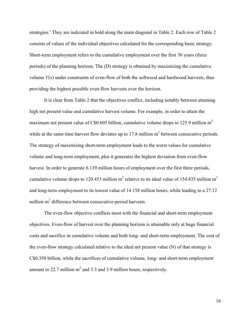
strategies.’ They are indicated in bold along the main diagonal in Table 2. Each row of Table 2

consists of values of the individual objectives calculated for the corresponding basic strategy.

Short-term employment refers to the cumulative employment over the first 30 years (three

periods) of the planning horizon. The (D) strategy is obtained by maximizing the cumulative

volume V(x) under constraints of even-flow of both the softwood and hardwood harvests, thus

providing the highest possible even-flow harvests over the horizon.

It is clear from Table 2 that the objectives conflict, including notably between attaining

high net present value and cumulative harvest volume. For example, in order to attain the

maximum net present value of C$0.605 billion, cumulative volume drops to 125.9 million m3

while at the same time harvest flow deviates up to 17.8 million m3 between consecutive periods.

The strategy of maximizing short-term employment leads to the worst values for cumulative

volume and long-term employment, plus it generates the highest deviation from even-flow

harvest. In order to generate 6.139 million hours of employment over the first three periods,

cumulative volume drops to 120.453 million m3 relative to its ideal value of 154.835 million m3

and long-term employment to its lowest value of 14.158 million hours, while leading to a 27.12

million m3 difference between consecutive-period harvests.

The even-flow objective conflicts most with the financial and short-term employment

objectives. Even-flow of harvest over the planning horizon is attainable only at huge financial

costs and sacrifice in cumulative volume and both long- and short-term employment. The cost of

the even-flow strategy calculated relative to the ideal net present value (N) of that strategy is

C$0.358 billion, while the sacrifices of cumulative volume, long- and short-term employment

amount to 22.7 million m3 and 3.3 and 3.9 million hours, respectively.

16

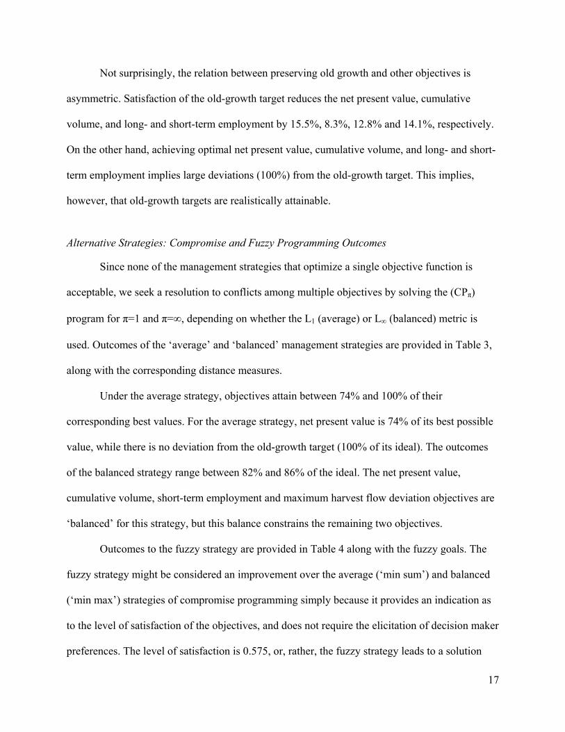
Not surprisingly, the relation between preserving old growth and other objectives is

asymmetric. Satisfaction of the old-growth target reduces the net present value, cumulative

volume, and long- and short-term employment by 15.5%, 8.3%, 12.8% and 14.1%, respectively.

On the other hand, achieving optimal net present value, cumulative volume, and long- and short-

term employment implies large deviations (100%) from the old-growth target. This implies,

however, that old-growth targets are realistically attainable.

Alternative Strategies: Compromise and Fuzzy Programming Outcomes

Since none of the management strategies that optimize a single objective function is

acceptable, we seek a resolution to conflicts among multiple objectives by solving the (CPπ)

program for π=1 and π=∞, depending on whether the L1 (average) or L∞ (balanced) metric is

used. Outcomes of the ‘average’ and ‘balanced’ management strategies are provided in Table 3,

along with the corresponding distance measures.

Under the average strategy, objectives attain between 74% and 100% of their

corresponding best values. For the average strategy, net present value is 74% of its best possible

value, while there is no deviation from the old-growth target (100% of its ideal). The outcomes

of the balanced strategy range between 82% and 86% of the ideal. The net present value,

cumulative volume, short-term employment and maximum harvest flow deviation objectives are

‘balanced’ for this strategy, but this balance constrains the remaining two objectives.

Outcomes to the fuzzy strategy are provided in Table 4 along with the fuzzy goals. The

fuzzy strategy might be considered an improvement over the average (‘min sum’) and balanced

(‘min max’) strategies of compromise programming simply because it provides an indication as

to the level of satisfaction of the objectives, and does not require the elicitation of decision maker

preferences. The level of satisfaction is 0.575, or, rather, the fuzzy strategy leads to a solution

17

that has a membership value of 0.575 in the set ‘all objectives have been optimized’. This is not a

resounding level of satisfaction and is, rather, indicative of the difficulty in balancing these

conflicting objectives.

The fuzzy strategy increases net discounted revenues (that can be used to fund economic

development) over the average strategy but slightly less than under the balanced strategy. The

sacrifice in terms of the old-growth target is very small – it achieves 91% of its ideal or best

possible value. Short-term employment attains some 80% of its best possible value, while other

objectives achieve more that 85% of their ideal values.

Dynamic Profile of Model Outcomes

Objective values are not always an adequate indicator of the usefulness of any given

forest management strategy. Rather, it is helpful to examine the profile of outcomes over time.

Here again, we expect the fuzzy strategy to provide the better option for decision makers, but we

compare it to the two compromise strategies to determine if this is indeed the case.

Harvest Flow

Consider first annual harvests per period assuming that decision makers focus on only

one objective at a time. As indicated in Figure 3, depending on which objective is chosen,

harvests will be constant over time (minimize deviation of harvests between decades), take place

almost entirely in the first thirty years of the planning horizon (maximize short-term

employment), or assume a pattern of significant fluctuation over time (other objectives). In all

cases except even-flow, harvests are projected to cease for a significant period beginning as early

as the fourth decade. Cessation of harvests is avoided in the even-flow case only because harvest

18

levels are depressingly low from an economic development point of view. Can a compromise or

fuzzy strategy lead to outcomes that avoid this possibility?

Harvest levels for the compromise and fuzzy strategies are provided in Figure 4. The

good news is that, even though harvest levels in each of the first decades are declining, the

compromise and fuzzy strategies are able to delay total cessation of harvests to at least the fifth

decade, while maintaining harvest levels above that under the current even-flow regime for at

least thirty years. This suggests that, while a downfall in timber harvests is unavoidable, harvest

levels might be sufficiently high that they could be relied upon as a driver of economic

development for perhaps 20 to 30 years, after which the local economy must be diversified if the

aboriginal community is to survive. This conclusion is reinforced by the models’ projections

concerning employment.

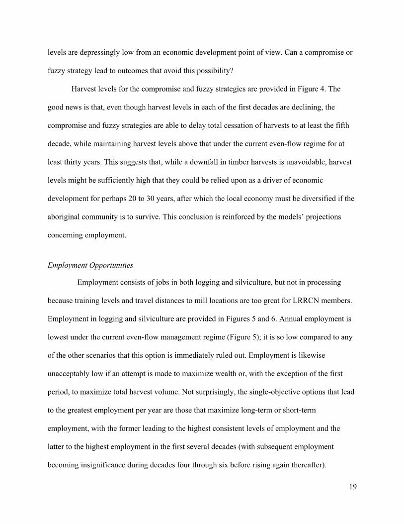
Employment Opportunities

Employment consists of jobs in both logging and silviculture, but not in processing

because training levels and travel distances to mill locations are too great for LRRCN members.

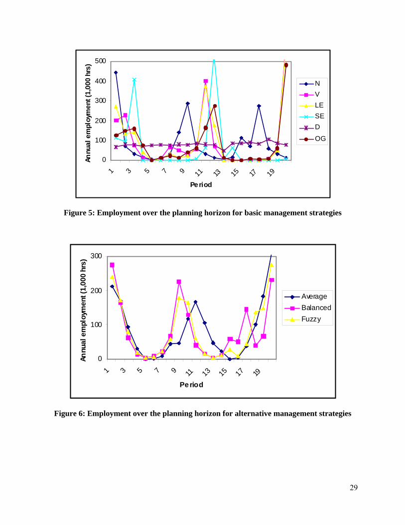
Employment in logging and silviculture are provided in Figures 5 and 6. Annual employment is

lowest under the current even-flow management regime (Figure 5); it is so low compared to any

of the other scenarios that this option is immediately ruled out. Employment is likewise

unacceptably low if an attempt is made to maximize wealth or, with the exception of the first

period, to maximize total harvest volume. Not surprisingly, the single-objective options that lead

to the greatest employment per year are those that maximize long-term or short-term

employment, with the former leading to the highest consistent levels of employment and the

latter to the highest employment in the first several decades (with subsequent employment

becoming insignificance during decades four through six before rising again thereafter).

19

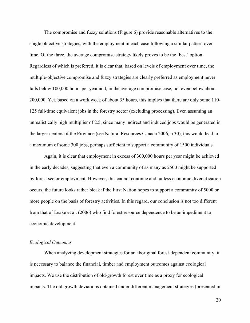
The compromise and fuzzy solutions (Figure 6) provide reasonable alternatives to the

single objective strategies, with the employment in each case following a similar pattern over

time. Of the three, the average compromise strategy likely proves to be the ‘best’ option.

Regardless of which is preferred, it is clear that, based on levels of employment over time, the

multiple-objective compromise and fuzzy strategies are clearly preferred as employment never

falls below 100,000 hours per year and, in the average compromise case, not even below about

200,000. Yet, based on a work week of about 35 hours, this implies that there are only some 110-

125 full-time equivalent jobs in the forestry sector (excluding processing). Even assuming an

unrealistically high multiplier of 2.5, since many indirect and induced jobs would be generated in

the larger centers of the Province (see Natural Resources Canada 2006, p.30), this would lead to

a maximum of some 300 jobs, perhaps sufficient to support a community of 1500 individuals.

Again, it is clear that employment in excess of 300,000 hours per year might be achieved

in the early decades, suggesting that even a community of as many as 2500 might be supported

by forest sector employment. However, this cannot continue and, unless economic diversification

occurs, the future looks rather bleak if the First Nation hopes to support a community of 5000 or

more people on the basis of forestry activities. In this regard, our conclusion is not too different

from that of Leake et al. (2006) who find forest resource dependence to be an impediment to

economic development.

Ecological Outcomes

When analyzing development strategies for an aboriginal forest-dependent community, it

is necessary to balance the financial, timber and employment outcomes against ecological

impacts. We use the distribution of old-growth forest over time as a proxy for ecological

impacts. The old growth deviations obtained under different management strategies (presented in

20

Tables 2, 3 and 4) provide information about maximum deviations from the old-growth target.

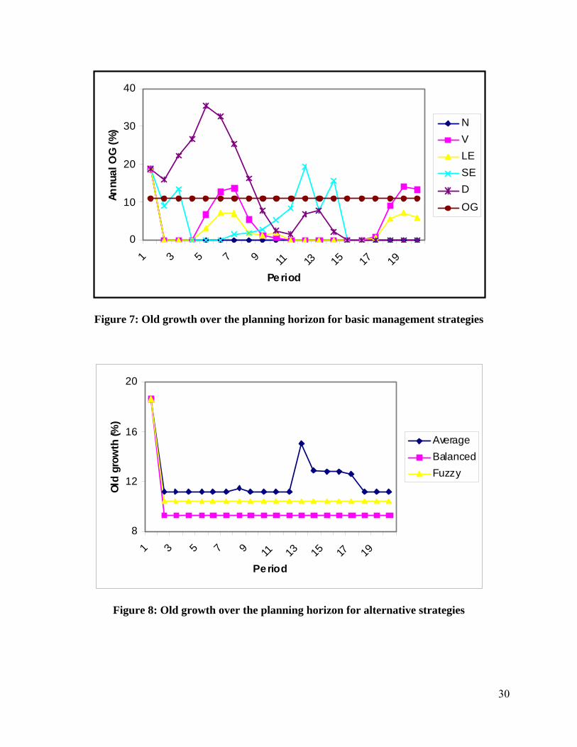
More detailed insights are obtained by analyzing old growth over time for different strategies.

For each of the several management strategies, the distribution of old forest over time is plotted

in Figures 7 and 8. The area of old-growth forest disappears entirely after the initial period under

the management strategies that maximize discounted net revenue, cumulative volume or long-

term employment. Under the short-term employment strategy, the amount of old growth remains

near the target amount. It is interesting that Alberta’s current sustained-yield forest policy (which

requires even-flow harvest) does not preserve old growth in the long run. After the seventh

decade, the amount of old growth drops below the target and never recovers (Figure 7).

The distribution of old-growth forest over time under alternative strategies is provided in

Figure 8. A deep plunge in the relative area of old growth in the second period is followed by

‘equilibrium’ for the three strategies. The balanced and fuzzy strategies provide a stable level of

old growth, but below the target amount. In contrast, the amount of old growth under the average

strategy is at or above the target over the entire planning horizon. The alternatives strategies

provide multiple socio-economic benefits, while at the same time making possible preservation

of old forests over time.

Discussion and Conclusions

In this study, we sought to determine whether the forest resources available to one

aboriginal forest-dependent community were sufficient to enable the community to develop or, at

minimum, retain an economic base for its members. Treaty 8 obligations appear to require that

the community have such rights, including forest resources that satisfy cultural needs (for which

we used proportion of old-growth forest as a proxy measure).

21

We also looked at the use of compromise and fuzzy programming methods for analyzing

conflicting objectives. The programming methods that we use are highly appropriate for the

problem at hand. They indicate that not all objectives can be satisfied and, indeed, that the

conflict among objectives is so great that, on a 0 to 1 scale, they can only be satisfied to a degree

less than 0.6.

Strategies that rely on intensive harvest activities at the beginning of the horizon may

enable the First Nation to achieve high financial returns without sacrificing future use of forest

resources. For example, sustainable management with a lax harvest flow regime offers an

opportunity for greater financial returns at the beginning of the planning horizon, which could be

diverted for building technical and professional capacity to be used by current and future

generations. Nonetheless, while this study sought to provide the best possible strategies that

might be available for a timber-dependent aboriginal community in northern Canada, no

management strategy is able to satisfy all of the technical, environmental and social/cultural

constraints and, at the same time, offer aboriginal peoples forest-based economic development.

Indeed, even if environmental and socio-cultural constraints were relaxed, economic

development based on timber resources would not be possible without significant reductions in

the population to be supported.

Acknowledgement

The authors wish to thank Dave Cole, Stephanie Grocholski and Ron Laframboise of the

Little Red River Forestry (LRRF), who provided useful insights and data during an on-site visit

and numerous telephone calls. Remaining errors are ours. We also want to thank SFM for

funding support.

22

References

Ballestero, E., 1997. “Selecting the CP Metric: A Risk Aversion Approach.” European Journal

of Operational Research 97: 593-596.

Brooke, A., D. Kendrick, A. Meeraus and R. Raman, 1998. GAMS. A User’s Guide. Washington,

DC: GAMS Development Corporation.

Burton, P., D. Kneeshaw and D. Coates, 1999. “Managing Forest Harvesting to Maintain Old

Growth in Boreal and Sub-boreal Forests.” The Forestry Chronicle 75: 623-631.

Jones, D.F. and M. Tamiz, 2003. “Analysis of Trends in Distance Metric Optimization Modeling

for Operations Research and Soft Computing.” In T. Tanino, T. Tanaka and M. Inuiguchi

(eds.) Multi-objective Programming and Goal-Programming. New York NY: Springer-

Verlag. pp.19-26.

Krcmar, E. and G.C. van Kooten, 2007. Economic Development Prospects of Forest-Dependent

Communities: Analyzing Tradeoffs using a Compromise-Fuzzy Programming

Framework. REPA Working Paper 2007-03. Victoria: Department of Economics.

Krcmar, E., G.C. van Kooten and I. Vertinsky, 2005. “Managing Forests for Multiple Tradeoffs:

Compromising On Timber, Carbon Uptake and Biodiversity Objectives.” Ecological

Modelling 185: 451-468.

Leake, N., W.L. Adamowicz and P.C. Boxall, 2006. “An Econometric Analysis of the Effects of

Forest Dependence on the Economic Well-Being of Canadian Communities.” Forest

Science 52(5): 595-604.

MOU (Memorandum of Understanding), 1996. Little Red River Cree Nation – Tall Cree Nation

and the Government of Alberta Cooperative Management Agreement. Albertat

Department of Aboriginal Affairs, Edmonton, Canada.

23

MOU (Memorandum of Understanding), 1999. Little Red River Cree Nation – Tall Cree Nation

and the Government of Alberta Cooperative Management Agreement. Alberta

Department of Aboriginal Affairs, Edmonton, Canada.

Natural Resources Canada, 2006. The State of Canada’s Forests 2005-2006. Forest Industry

Competitiveness. Ottawa: Canadian Forest Service, Natural Resources Canada.

Romero, C., M. Tamiz, and D.F. Jones, 1998. “Goal Programming, Compromise Programming

and Reference Point Method Formulations: Linkages and Utility Interpretations.” Journal

of the Operational Research Society 49: 986-991.

Spies, T.A. and J.F. Franklin, 1996. “The Diversity and Maintenance of Old-growth Forests.” In

Szaro, R.C. and D.W. Johnston (eds.) Biodiversity in Managed Landscapes. Oxford

University Press, Oxford. UK, 296-314.

Walkem, A., 1994. First Nations and Old Growth Values. Spence's Bridge, BC: Cook's Ferry

Band.

Wierzbicki, A.P., 1999. “Reference Point Approaches.” In T. Gal, T.J. Stewart and T. Hanne,

(eds.) Multicriteria Decision Making: Advances in MCDM Models, Algorithms, Theory

and Applications. Dordrecht, NL: Kluwer Academic Publishers. pp. 9.1-9.39.

Yu, P.L., 1973. “A Class of Solutions for Group Decision Problems.” Management Science 19:

936-946.

Zimmermann, H.-J., 1978. “Fuzzy Programming and Linear Programming with Several

Objective Functions.” Fuzzy Sets and Systems 1: 45-55.

24

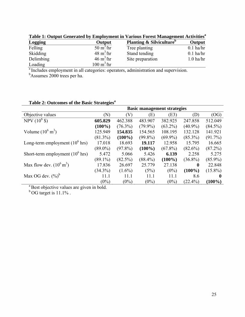
Table 1: Output Generated by Employment in Various Forest Management Activitiesa Logging Output Planting & Silvicultureb OutputFelling 50 m3/hr Tree planting 0.1 ha/hrSkidding 48 m3/hr Stand tending 0.1 ha/hrDelimbing 46 m3/hr Site preparation 1.0 ha/hrLoading 100 m3/hr a Includes employment in all categories: operators, administration and supervision. bAssumes 2000 trees per ha.

Table 2: Outcomes of the Basic Strategiesa

Basic management strategies Objective values (N) (V) (E) (E3) (D) (OG)NPV (106 $) 605.829

(100%)462.388 (76.3%)

483.907 (79.9%)

382.925 (63.2%)

247.858 (40.9%)

512.049 (84.5%)

Volume (106 m3) 125.949 (81.3%)

154.835(100%)

154.565(99.8%)

108.195 (69.9%)

132.128(85.3%)

141.921(91.7%)

Long-term employment (106 hrs) 17.018(89.0%)

18.693(97.8%)

19.117(100%)

12.958 (67.8%)

15.795(82.6%)

16.665(87.2%)

Short-term employment (106 hrs) 5.472(89.1%)

5.066(82.5%)

5.426(88.4%)

6.139 (100%)

2.258(36.8%)

5.275(85.9%)

Max flow dev. (106 m3) 17.836(34.3%)

26.697(1.6%)

25.779(5%)

27.138 (0%)

0(100%)

22.848(15.8%)

Max OG dev. (%)b 11.1 (0%)

11.1 (0%)

11.1 (0%)

11.1 (0%)

8.6(22.4%)

0(100%)

a Best objective values are given in bold. b OG target is 11.1% .

25

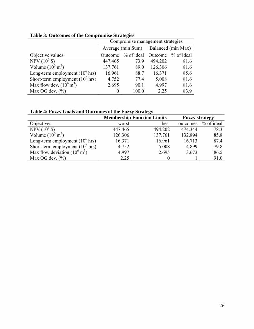
Table 3: Outcomes of the Compromise Strategies Compromise management strategies Average (min Sum) Balanced (min Max) Objective values Outcome % of ideal Outcome % of ideal NPV (106 $) 447.465 73.9 494.202 81.6 Volume (106 m3) 137.761 89.0 126.306 81.6 Long-term employment (106 hrs) 16.961 88.7 16.371 85.6 Short-term employment (106 hrs) 4.752 77.4 5.008 81.6 Max flow dev. (106 m3) 2.695 90.1 4.997 81.6 Max OG dev. (%) 0 100.0 2.25 83.9

Table 4: Fuzzy Goals and Outcomes of the Fuzzy Strategy Membership Function Limits Fuzzy strategy Objectives worst best outcomes % of idealNPV (106 $) 447.465 494.202 474.344 78.3Volume (106 m3) 126.306 137.761 132.894 85.8Long-term employment (106 hrs) 16.371 16.961 16.713 87.4Short-term employment (106 hrs) 4.752 5.008 4.899 79.8Max flow deviation (106 m3) 4.997 2.695 3.673 86.5Max OG dev. (%) 2.25 0 1 91.0

26

Figure 1: The study area (in green) relative to the Province of Alberta

N(x) (mil $)N2N1

μN(x)

1

N(x) (mil $)N2N1

μN(x)

1

D(x) (mil. m3)D2D1

μD(x)

1

D(x) (mil. m3)D2D1

μD(x)

1

(a)

(b)

N(x) (mil $)N2N1

μN(x)

1

N(x) (mil $)N2N1

μN(x)

1

D(x) (mil. m3)D2D1

μD(x)

1

D(x) (mil. m3)D2D1

μD(x)

1

(a)

(b) Figure 2: Membership function for (a) net discount returns, N(x); and (b) deviation in

between period harvests, D(x).

27

0

1000

2000

3000

4000

1 3 5 7 9 11 13 15 17 19

Period

Ann

ual h

arve

st (1

,000

m3)

NVLESEDOG

Figure 3: Harvest flow over the planning horizon for basic management strategies

0

500

1000

1500

2000

2500

1 3 5 7 9 11 13 15 17 19

Period

Annu

al h

arve

st (1

,000

m3)

AverageBalancedFuzzy

Figure 4: Harvest flow the planning horizon for alternative management strategies

28

0

100

200

300

400

500

1 3 5 7 9 11 13 15 17 19

Period

Annu

al e

mpl

oym

ent (

1,00

0 hr

s)NVLESED

OG

Figure 5: Employment over the planning horizon for basic management strategies

0

100

200

300

1 3 5 7 9 11 13 15 17 19

Period

Annu

al e

mpl

oym

ent (

1,00

0 hr

s)

AverageBalancedFuzzy

Figure 6: Employment over the planning horizon for alternative management strategies

29

0

10

20

30

40

1 3 5 7 9 11 13 15 17 19

Period

Annu

al O

G (%

) NVLESED

OG

Figure 7: Old growth over the planning horizon for basic management strategies

8

12

16

20

1 3 5 7 9 11 13 15 17 19

Period

Old

grow

th (%

)

AverageBalancedFuzzy

Figure 8: Old growth over the planning horizon for alternative strategies

30