OPTIMAL DRIVELINE ROBOT BASE

Development of a driveline with low speed maneuverability and high speed stability

Submitted in partial fulfillment of the Bachelor of Science degree of

Worcester Polytechnic Institute, Worcester, MA

Submitted to: Prof Kenneth Stafford (advisor) Prof Taskin Padir (co-advisor)

Michael Cullen (ME) _____________________________________

Stephen Diamond (RBE/ECE) _____________________________________

William Dunn (RBE) _____________________________________

Kirk Gimsley (RBE) _____________________________________

Submitted on: May 1st, 2014 ___________________________________

Advisor Signature

___________________________________

Co-advisor Signature

1

Authorship The Background and Design Goals were written by all group members collaboratively. The other

sections of this report were primarily written by individual members as specified below.

Name Contributions

Michael Cullen Manufacturing- Steering Assembly, Design- Steering Assembly, Testing & Evaluation, Results

Stephen Diamond Design- Electrical and Programming, Budget, Schematic, Manufacturing- Programming Implementation

William Dunn Manufacturing- Chassis, Manufacturing- Wheel Modules, Design- Chassis, Design- Wheel Modules, Social Implications, Discussion, Results

Kirk Grimsley Manufacturing- Electrical Systems, Manufacturing- Programming, Executive Summary, Design Selection, Discussion, Final Conclusions

2

Abstract

Our team has decided that there is currently a need for a driveline system that is capable of

performing a zero radius turn and being maneuverable at low speeds while also maintaining

traction, stability, and energy efficiency at high speeds. We designed and prototyped a modified

Ackermann steering system driven by a single motor, with an extended range of motion. This

driveline system also enforces that all wheels are driven in all conditions. The steering system

was integrated into a robot chassis that meets FRC requirements.

3

Table of Contents AUTHORSHIP............................................................................................................................................ 1

ABSTRACT ................................................................................................................................................ 2

TABLE OF FIGURES ................................................................................................................................... 5

EXECUTIVE SUMMARY ............................................................................................................................. 6

BACKGROUND.......................................................................................................................................... 8

EXISTING DRIVE SYSTEMS .................................................................................................................................. 8

Ackermann Steering ................................................................................................................................ 8

Holonomic Drive ...................................................................................................................................... 9

Swerve Drive ......................................................................................................................................... 11

Tank Drive ............................................................................................................................................. 12

Chassis Steering .................................................................................................................................... 13

FIRST ROBOTICS ........................................................................................................................................... 14

FIRST Constraints .................................................................................................................................. 14

Team 190 Survey ................................................................................................................................... 15

Past FRC Designs ................................................................................................................................... 15

DESIGN GOALS ....................................................................................................................................... 18

PRIMARY GOALS ............................................................................................................................................ 18

High-Speed Stability .............................................................................................................................. 18

Low-Speed Maneuverability ................................................................................................................. 18

GENERAL GOALS ............................................................................................................................................ 18

PROJECT DESIGN .................................................................................................................................... 20

DESIGN SELECTION ......................................................................................................................................... 20

MECHANICAL SYSTEMS ................................................................................................................................... 23

Steering Assembly ................................................................................................................................. 23

Wheel Modules ..................................................................................................................................... 29

Chassis .................................................................................................................................................. 36

ELECTRICAL SYSTEMS ...................................................................................................................................... 38

Motor Selections ................................................................................................................................... 38

Sensors .................................................................................................................................................. 40

Teleoperation ........................................................................................................................................ 41

Schematic .............................................................................................................................................. 41

PROGRAMMING ............................................................................................................................................. 42

Motor Control ....................................................................................................................................... 42

Pseudo code .......................................................................................................................................... 43

BUDGET ....................................................................................................................................................... 44

MANUFACTURING AND ASSEMBLY ........................................................................................................ 46

MECHANICAL SYSTEMS ................................................................................................................................... 46

Chassis .................................................................................................................................................. 46

Front Wheel Modules ............................................................................................................................ 48

4

Rear Wheel Modules ............................................................................................................................. 50

Steering Assembly ................................................................................................................................. 51

ELECTRICAL ASSEMBLY .................................................................................................................................... 55

PROGRAMMING IMPLEMENTATION .................................................................................................................... 57

TESTING AND EVALUATION .................................................................................................................... 60

INDIVIDUAL PERFORMANCE EVALUATION ............................................................................................................ 60

COMPARATIVE PERFORMANCE EVALUATION ........................................................................................................ 60

CONCLUSION ......................................................................................................................................... 62

RESULTS ....................................................................................................................................................... 62

DISCUSSION .................................................................................................................................................. 63

SOCIAL IMPLICATIONS ..................................................................................................................................... 65

FINAL CONCLUSIONS ....................................................................................................................................... 66

APPENDICES ........................................................................................................................................... 67

APPENDIX A: DRIVER PERFORMANCE COURSE DATA .............................................................................................. 67

APPENDIX B: CODE......................................................................................................................................... 67

APPENDIX C: FRC MOTOR DATA ...................................................................................................................... 77

APPENDIX D: POWER REQUIREMENT DATA ......................................................................................................... 77

APPENDIX E: BOSCH VAN DOOR MOTOR OUTPUT DATA ....................................................................................... 78

5

Table of Figures FIGURE 1: ACKERMANN STEERING .............................................................................................................................................. 9

FIGURE 2: MECANUM WHEEL.................................................................................................................................................. 10

FIGURE 3: MECANUM DRIVE .................................................................................................................................................. 10

FIGURE 4: SWERVE DRIVE FRAME ............................................................................................................................................ 11

FIGURE 5: SWERVE DRIVE - CLOSE-UP CONFIGURATION ................................................................................................................ 12

FIGURE 6: TRADITIONAL ZERO-TURN LAWNMOWER ..................................................................................................................... 13

FIGURE 7: 2013 "ULTIMATE FUNKY OBJECT" BY LYNBROOK ROBOTICS ............................................................................................ 15

FIGURE 8: ROBOWRANGLERS 2008 FRC ROBOT, "TUMBLEWEED" ................................................................................................. 16

FIGURE 9: CONCEPTUAL AMPLIFIED ACKERMANN STEERING ............................................................................................................ 24

FIGURE 10: ZERO RADIUS TURNING CONDITIONS.......................................................................................................................... 24

FIGURE 11: TRAPEZOIDAL STEERING GEOMETRY .......................................................................................................................... 25

FIGURE 12: DESIGNED VERSUS PERFECT ACKERMANN PLOT ............................................................................................................ 27

FIGURE 13: CONCEPTUAL STEERING ARM DESIGN ......................................................................................................................... 27

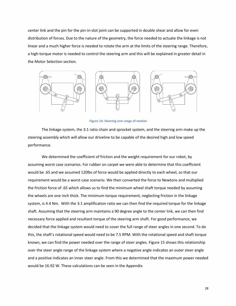
FIGURE 14: STEERING ARM RANGE OF MOTION ........................................................................................................................... 28

FIGURE 15: REQUIRED STEERING ARM POWER ............................................................................................................................. 29

FIGURE 16: ANDYMARK WILD SWERVE DRIVE MODULE ............................................................................................................... 31

FIGURE 17: ORIGINAL BRACKET ASSEMBLY ................................................................................................................................. 32

FIGURE 18: MODIFIED BRACKET ASSEMBLY ................................................................................................................................ 32

FIGURE 19: PARTIAL KIT FOR REAR WHEELS ................................................................................................................................ 33

FIGURE 20: FINAL MODIFIED WILD SWERVE MODULE FOR FRONT WHEELS ......................................................................................... 34

FIGURE 21: NEW 22 TOOTH SPROCKET WITH HOLES DRILLED .......................................................................................................... 34

FIGURE 22: MODIFIED SPROCKET ASSEMBLY ............................................................................................................................... 35

FIGURE 23: PART DRAWING FOR REAR WHEEL MODULE PLATE......................................................................................................... 35

FIGURE 24: OFF-THE-SHELF VEX CHASSIS .................................................................................................................................. 36

FIGURE 25: CHASSIS DESIGN WITH VEX ANGLE BARS .................................................................................................................... 37

FIGURE 26: FINAL CAD MODEL ............................................................................................................................................... 38

FIGURE 27: VAN DOOR MOTOR OUTPUT TORQUE ........................................................................................................................ 40

FIGURE 28: ELECTRICAL SCHEMATIC.......................................................................................................................................... 42

FIGURE 29: LIST OF EXPENSES ................................................................................................................................................. 45

FIGURE 30: PARTIAL FRAME DURING ASSEMBLY ........................................................................................................................... 47

FIGURE 31: COMPLETED FRAME WITH WHEEL MODULES ................................................................................................................ 47

FIGURE 32: SPROCKET ASSEMBLY COMPONENTS .......................................................................................................................... 48

FIGURE 33: MODIFIED SPROCKET ASSEMBLY ............................................................................................................................... 49

FIGURE 34: COMPLETED ASSEMBLY IN PLACE .............................................................................................................................. 50

FIGURE 35: CAD FOR WHEEL SHAFT ......................................................................................................................................... 51

FIGURE 36: COMPLETED REAR WHEEL ASSEMBLY ......................................................................................................................... 51

FIGURE 37: TIE ROD (TOP) AND STEERING ARM (BOTTOM) ............................................................................................................. 52

FIGURE 38: PLATE SPROCKETS WITH SLOTS (LEFT) AND TIE ROD/SPROCKET ASSEMBLY (RIGHT) ................................................................ 53

FIGURE 39: MANUFACTURED STEERING ASSEMBLY WITH STANDOFFS ................................................................................................ 53

FIGURE 40: NEW STEERING ARM ASSEMBLY ................................................................................................................................ 54

FIGURE 41: COMPLETED ROBOT DRIVELINE AND CHASSIS ............................................................................................................... 54

FIGURE 42: A PICTURE OF OUR POTENTIOMETER WITH THE 3D PRINTED ADAPTER TO THE TURNING MOTOR. ............................................. 57

FIGURE 43: WHEEL VELOCITY VS. STEER ANGLE ........................................................................................................................... 59

FIGURE 44: PERFORMANCE COURSE ......................................................................................................................................... 61

FIGURE 45: AVERAGE DRIVER COURSE TIMES .............................................................................................................................. 63

6

Executive Summary Our team has analyzed different frequently used drivelines and determined that they all

have distinct weaknesses that we could improve upon. The most commonly used driveline on a

robotic chassis, especially for FIRST Robots, which we will be what we compare our system to, is

tank drive. This style of driving has two significant drawbacks: an inability to handle well at high

speed, and, since it turns via skid steer, it is very energy inefficient. Another is swerve drive,

which is extremely maneuverable and can be programmed so that it handles well, but takes a

significant number of motors, a lot of programming and a high level of user skill to operate well.

The type of steering most people will be familiar with is Ackermann steering, which is what a

traditional car uses. The issue with a car is that even though it handles extremely well at high

speeds, at lower speeds it requires significant effort to make precise, small radius turns.

Based on this analysis we set about creating a system that would be able to maintain

high speed handling, low speed maneuverability, and maximize energy efficiency by reducing

wheel skid. To do this we evaluated different options for drivelines and determined that the one

that best met our requirements was an “Enhanced Ackermann” system. This system would use a

standard car Ackermann, but we would modify the wheels and the tie rod linkage so that they

would turn 147° instead of the approximately 60° a normal car can turn. This allows us to reduce

the radius of the circle the driveline is turning about, until it is turning about one of the back

wheels. Therefore, when making a left hand turn, our chassis pivots about the back left wheel

and when making a right hand turn, it pivots about the right rear wheel. In order to do this we

had to use specific geometry to make sure the wheel angles changed at the proper ratios to one

another, as wheel as create wheel speed algorithms to determine how fast each individual

wheel should be spinning depending on how tight any given turn is.

Once we implemented our system we were able to drive it through a course and

compare the number of obstacles hit, and time to run the course. We also evaluated a typical

skid-steered FRC robot with the same drivers. During this testing our robot was slightly slower

than the FRC robot and it also hit more obstacles. However, upon discussing the results of the

driving with the participants we found that they were all extremely happy with the handling and

mechanical systems of our driveline. Instead, we found that they felt the majority of the reason

for the setbacks was the remote control system being used. We had opted for an RC airplane

style controller, and most felt the range of motion available to the joysticks was too small to

7

allow for easy handling of our system. Based on this feedback and the results we saw, we feel

that mechanically our chassis was able to meet all of the requirements, but that the user

interface needed additional time to properly implement and optimize for our system. Of the

initial goals we set out to achieve, the only one we failed to meet was to complete the course

faster than a traditional FRC robot. We were able to accomplish the goals of reaching a speed of

at least 10 ft/sec, maintaining a 4 foot lane while driving a 10 foot radius circle, being able to

turn about a point within the perimeter of the chassis, maximizing for traction at lower speeds

by driving all wheels, maximizing energy efficiency by minimizing skidding, and complying with

all rules and requirements from the FRC 2013 season.

8

Background

Existing Drive Systems

Ackermann Steering

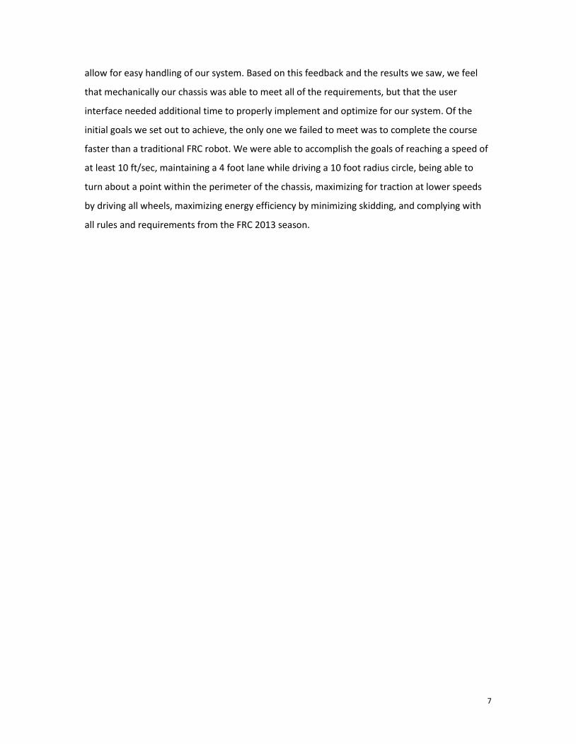
Ackermann steering is based on the fact that when a vehicle goes around a turn, the wheels

on the outside have to travel farther, and they follow a different arc than the wheels on the

inside of the turn. Modern cars do not use a pure Ackermann steering due to some limitations in

high-speed maneuvers. Race cars use a reverse Ackermann steering which is better for high

speed maneuvers.

During traditional Ackermann steering, each of the four wheels must spin at a different

speed to prevent skidding. The front tires tend to spin at a faster rate than the rear tires, and the

wheels on the outside of the turn must rotate faster than the inside wheels. So for a left turn,

the right-front tire spins the fastest out of the four while the left rear tire spins the slowest.

This is accomplished by differentials and different turning angles for each front wheel. Since

the axes of all four wheels must be oriented toward the point about which the vehicle is turning,

the two front tires pivot at different angles for any given turn while the rear wheels remain fixed

to their shared axle. For a left turn, the left front wheel is turned at a different angle than the

right front wheel because of the different arc that each wheel needs to make in order to prevent

tire slip.

9

Figure 1: Ackermann Steering

Triple Differential

A triple differential is needed in order for Ackermann steering to function with all-wheel

drive (AWD) systems. Without a triple differential, problems can occur due to transmission wind

up or lock up due to the tires not being able to spin at different speeds around corners.

A triple differential is setup with a differential on both the front and rear axles and an

additional differential on the drive shaft coming from the transmission or transfer case. The

differentials on the axles allow the wheels to spin at different speeds around corners, which

prevents tire slip. However, a center differential is also required to allow the front axle to travel

further than the rear axle to prevent transmission lock up around corners.

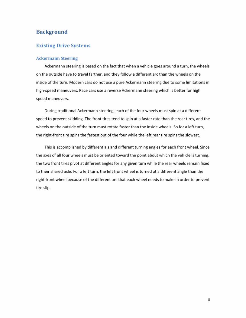
Holonomic Drive

The holonomic drive system uses multiple specialized wheels such that the robot can move

in any direction by running the wheels at different speeds. This provides a high degree of

maneuverability because the robot does not have to rotate its chassis or wheel modules before

moving in any given direction. Any direction of motion can be achieved simply by driving each

wheel at the correct speed. This requires the wheels to be able to slide laterally, so omni or

mechanum wheels are generally used.

10

Figure 2: Mecanum wheel

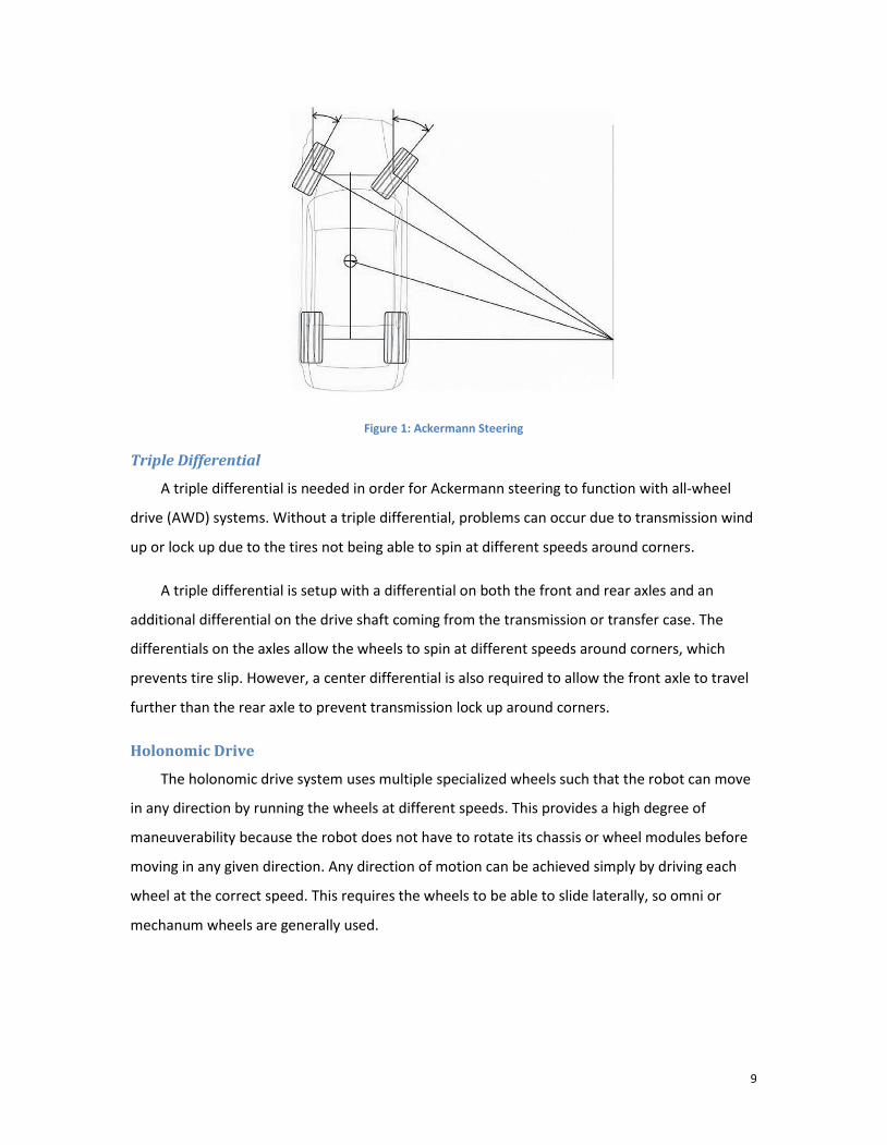
This drive system is not always intuitive, and controlling each wheel directly is difficult for

an operator. To make this easier to control, it is helpful to implement a solution on the firmware

level that uses the desired direction of motion to calculate the required speeds of each wheel.

This allows a holonomic drive robot to be controlled more easily.

Figure 3: Mecanum Drive

Mecanum-wheeled, holonomic drive robots are common due to the fact that they are

mechanically simple and extremely maneuverable at low speeds. The ability to achieve rotation

(zero turn radius) or translation in any direction immediately (without first having to turn the

11

robot) makes it very advantageous. The down side is that this system is relatively complex from

a control standpoint. Determining how to actually get the robot to move in a given direction

requires some calculations to be made. The fact that this cannot be implemented without

mecanum wheels is also problematic. A major detractor for this design is that roller wheels

which are required for this to operate severely limit the robot’s traction.

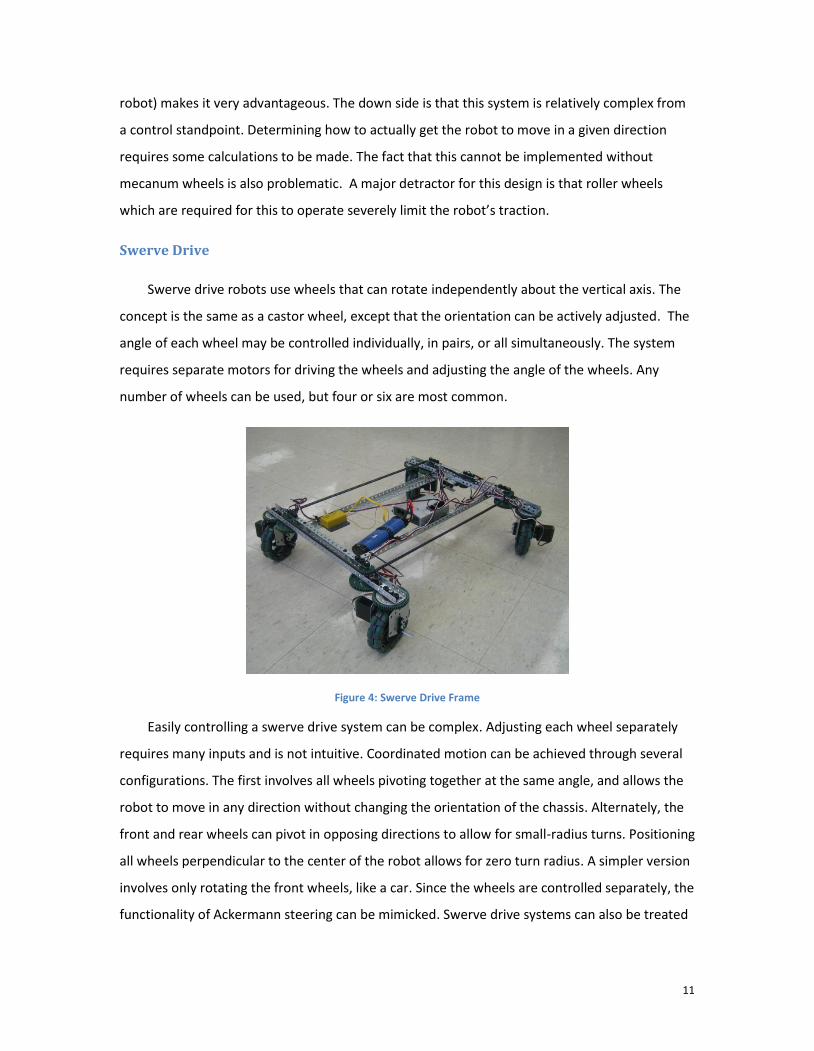
Swerve Drive

Swerve drive robots use wheels that can rotate independently about the vertical axis. The

concept is the same as a castor wheel, except that the orientation can be actively adjusted.  The

angle of each wheel may be controlled individually, in pairs, or all simultaneously. The system

requires separate motors for driving the wheels and adjusting the angle of the wheels. Any

number of wheels can be used, but four or six are most common.

Figure 4: Swerve Drive Frame

Easily controlling a swerve drive system can be complex. Adjusting each wheel separately

requires many inputs and is not intuitive. Coordinated motion can be achieved through several

configurations. The first involves all wheels pivoting together at the same angle, and allows the

robot to move in any direction without changing the orientation of the chassis. Alternately, the

front and rear wheels can pivot in opposing directions to allow for small-radius turns. Positioning

all wheels perpendicular to the center of the robot allows for zero turn radius. A simpler version

involves only rotating the front wheels, like a car. Since the wheels are controlled separately, the

functionality of Ackermann steering can be mimicked. Swerve drive systems can also be treated

12

exactly like tank-drive systems by allowing the wheels to remain parallel to each other and

driving one side faster or slower to turn.

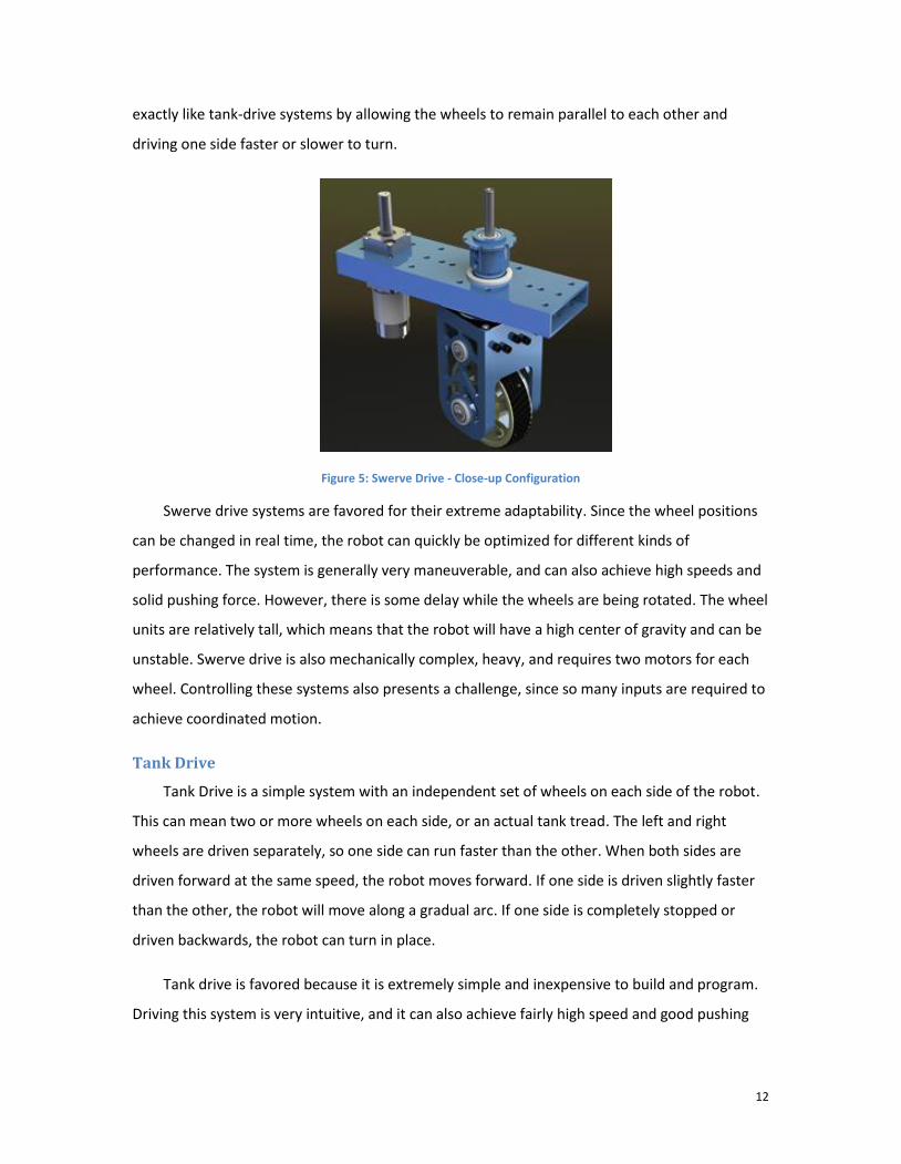
Figure 5: Swerve Drive - Close-up Configuration

Swerve drive systems are favored for their extreme adaptability. Since the wheel positions

can be changed in real time, the robot can quickly be optimized for different kinds of

performance. The system is generally very maneuverable, and can also achieve high speeds and

solid pushing force. However, there is some delay while the wheels are being rotated. The wheel

units are relatively tall, which means that the robot will have a high center of gravity and can be

unstable. Swerve drive is also mechanically complex, heavy, and requires two motors for each

wheel. Controlling these systems also presents a challenge, since so many inputs are required to

achieve coordinated motion.

Tank Drive

Tank Drive is a simple system with an independent set of wheels on each side of the robot.

This can mean two or more wheels on each side, or an actual tank tread. The left and right

wheels are driven separately, so one side can run faster than the other. When both sides are

driven forward at the same speed, the robot moves forward. If one side is driven slightly faster

than the other, the robot will move along a gradual arc. If one side is completely stopped or

driven backwards, the robot can turn in place.

Tank drive is favored because it is extremely simple and inexpensive to build and program.

Driving this system is very intuitive, and it can also achieve fairly high speed and good pushing

13

force. The downside is that this driveline requires the wheels to slip and skid frequently, which

drains power and makes it slightly less agile.

Chassis Steering

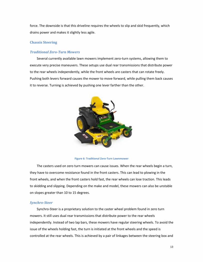
Traditional Zero-Turn Mowers

Several currently available lawn mowers implement zero-turn systems, allowing them to

execute very precise maneuvers. These setups use dual rear transmissions that distribute power

to the rear wheels independently, while the front wheels are casters that can rotate freely.

Pushing both levers forward causes the mower to move forward, while pulling them back causes

it to reverse. Turning is achieved by pushing one lever farther than the other.

Figure 6: Traditional Zero-Turn Lawnmower

The casters used on zero turn mowers can cause issues. When the rear wheels begin a turn,

they have to overcome resistance found in the front casters. This can lead to plowing in the

front wheels, and when the front casters hold fast, the rear wheels can lose traction. This leads

to skidding and slipping. Depending on the make and model, these mowers can also be unstable

on slopes greater than 10 to 15 degrees.

Synchro-Steer

Synchro-Steer is a proprietary solution to the caster wheel problem found in zero turn

mowers. It still uses dual rear transmissions that distribute power to the rear wheels

independently. Instead of two lap bars, these mowers have regular steering wheels. To avoid the

issue of the wheels holding fast, the turn is initiated at the front wheels and the speed is

controlled at the rear wheels. This is achieved by a pair of linkages between the steering box and

14

the rear transmissions. Rather than using casters, the front wheels are turned by the steering

wheel. When the steering wheel is turned clockwise (for example) the front wheels turn right,

and the power to the rear right wheel is decreased. The rear left wheel then pushes the mower

through the turn. This allows the mower to make zero radius turns intuitively in any situation.

FIRST Robotics

For Inspiration and Recognition of Science and Technology (FIRST) is an organization

founded by Dean Kamen. The organization, which was developed in 1989, is used to promote

and encourage students to enter engineering and technology based fields. The robotics side of

the organization is an international competition for high school students to compete. For this

competition, teams enter a robot which must be able to complete certain tasks for a game

which is determined every year. The robots must meet the rules and standards set forth by the

FIRST organization.

FIRST Constraints

Our group has decided to use the constraints set by the FIRST Robotics Competition for our

robot. Not only will this allow our design to be potentially used by future FIRST robotics teams

but it will also determine our constraints instead of arbitrarily coming up with our own. The

constraints determined by the FIRST organization cover a vast majority of the robot size and

weight specifications. Many of these regulations ensure that the robots entered are safe to

handle and fit particular size requirements. The rules described below are in regards to the rules

for the 2013 game, Ultimate Ascent.

These rules pertain to the size and weight of the robot. The robot should have a perimeter

that does not exceed 112 inches. The robot must also fit inside a 54 inch diameter cylinder. The

height shall not exceed 54 inches and the weight should be less than 120 pounds. The weight

measurement does not include the battery, cables pertaining to the power system, and the

bumpers.

The FIRST constraints will also give us a list of acceptable parts that can be added to the

robot such as sensors, motors, and controllers. This list of parts mainly applies to the accepted

motors. All electrical components used on the robot must also fit into the rules in regards to

wiring and their perspective actions.

15

Team 190 Survey

Since our group does not have any experience with FIRST or working within the guidelines

set forth by FIRST, we decided to go to one of Worcester Polytechnic Institute and Mass

Academy’s, FRC Team 190’s meeting. This allowed us to ask a few questions about robots

designed for FIRST Robotics Competitions. The questions dealt purely with the driveline of the

robot, which gave us a better idea of how much the driveline should weigh, what is the current

preferred driveline, and general performance of other drivelines used.

Past FRC Designs

In FIRST Robotics Competitions, many types of drivelines are used for the various types of

challenges that are created. The specific choice of what driveline to use is based on the needs of

the game created for that year’s competition. Most designs for the drivetrain focus on higher

pushing or pulling power as most of the games have some portion where an object must be

moved in some way, be it pushing, pulling, carrying, or some other method. The needs for high

speeds or maneuverability in the driveline design are also determined based on the goals of the

game. Most designs focus on either one of these based on the plan for the robot in the

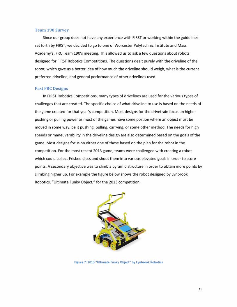
competition. For the most recent 2013 game, teams were challenged with creating a robot

which could collect Frisbee discs and shoot them into various elevated goals in order to score

points. A secondary objective was to climb a pyramid structure in order to obtain more points by

climbing higher up. For example the figure below shows the robot designed by Lynbrook

Robotics, “Ultimate Funky Object,” for the 2013 competition.

Figure 7: 2013 "Ultimate Funky Object" by Lynbrook Robotics

16

This drivetrain is a 6-wheel chain drive design which is capable of 15.7 feet per second. The

wheels are powered using 4 CIM motors and the gearbox used quickly shifts using servo motors

with feedback and synchronization. While this design is capable of high straight line speed and

zero-radius turning at a standstill, there are still some drawbacks of this design. At high speed

this design does not turn well due to the wheel configuration. It is also incapable of any form

translational movement meaning that the most effective way to drive this robot is drive in

straight lines, turn at a standstill, and continue on a desired path. For the game this was

designed for, this design was effective because it was quickly able to gather disks, move to

within range, and rotate the base in order to shoot and score points.

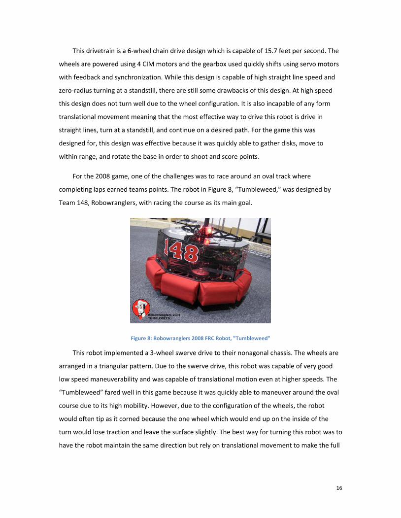
For the 2008 game, one of the challenges was to race around an oval track where

completing laps earned teams points. The robot in Figure 8, “Tumbleweed,” was designed by

Team 148, Robowranglers, with racing the course as its main goal.

Figure 8: Robowranglers 2008 FRC Robot, "Tumbleweed"

This robot implemented a 3-wheel swerve drive to their nonagonal chassis. The wheels are

arranged in a triangular pattern. Due to the swerve drive, this robot was capable of very good

low speed maneuverability and was capable of translational motion even at higher speeds. The

“Tumbleweed” fared well in this game because it was quickly able to maneuver around the oval

course due to its high mobility. However, due to the configuration of the wheels, the robot

would often tip as it corned because the one wheel which would end up on the inside of the

turn would lose traction and leave the surface slightly. The best way for turning this robot was to

have the robot maintain the same direction but rely on translational movement to make the full

17

turn. While this was effective for the challenge, in many other applications forcing translational

movement to turn around corners is sub optimal.

While these are just two examples of different robot designs for FRC, it provides some

important information regarding the differences of FIRST drivetrains and the drivetrain we will

build. The drivetrains used for different games are efficient because they are used to accomplish

certain goals for the challenge provided. However, these drivelines are not optimal as many

sacrifices are made due to time constraints and a need for simplicity. Therefore it is important to

recognize that while our design will use FRC design constraints, the driveline is not being made

for a FIRST competition. Sub-optimal drivelines will do just fine for most FIRST games but that is

not the goal of this project.

18

Design Goals

Primary Goals The concept of creating an optimal driveline is a very vague one. In order to make this

objective achievable, we must set design goals for us to be able to objectively determine that an

optimal driveline had been created. For our project, there are two main goals which must be

achieved in order classify our design as optimal. They are stability at high speeds and

maneuverability at low speeds. These two goals are still unspecific, so we have generated

criteria on which to grade success in these areas.

High-Speed Stability

For high speed stability, we have determined based on research into FIRST robotics

competitions that maintaining a speed higher than 10 feet per second can be classified as high

speed. With this definition of high speed established, we aimed to create a device which is

capable of two main operational goals at high speed. First, our drivetrain and chassis will be able

to maintain our definition of high speed around a circular path of a 4 foot lane with a 10 foot

radius. This test will prove that our design can maintain a constant turn radius without jerking

motions or the need to reposition. The radius of the circle was determined based on the 2008

FRC game “Overdrive” where the robots raced around a track on which the maximum turn

radius was 13.5 feet. Secondly, to test other practical high speed maneuvers, we decided to

create a slalom course on which to race FIRST robots. We gathered a group of FRC drivers with

various degrees of experience and have them drive the course several times, with our design

and with a driveline used by WPI and Mass Academy’s Team 190 in a previous competition. We

hoped that the majority of the selected drivers would finish the course faster with our design

than with Team 190’s driveline. By succeeding in both these tasks, we could successfully say our

driveline achieves high speed stability.

Low-Speed Maneuverability

To establish low speed maneuverability, the driveline must be capable of specific

operations at a standstill or very low speeds. First, our driveline will be capable of zero radius

turning about a point within the chassis. This will insure that our design has great

maneuverability at a standstill. Second, we wanted the driveline to be capable of precise

movements at low speeds. This can be accomplished with a design that is capable of

translational movement. However, translational movement is not a requirement because with

zero radius turning capability and straight line movement, we feel that these precise movements

are also feasible. With these objectives achieved, we can assure that our driveline has low speed

maneuverability.

General Goals Finally, there are some general goals we have established based on the FRC constraints and

engineering efficiency. We will maximize the tractive forces especially at low speeds and

maximize the energy efficiency of the driveline. The most effective way to do this is to make all

wheels driven and limit wheel skid. Our design will also comply with all FRC robot design

19

constraints from the 2013 competition. The target weight of the drivetrain and chassis is 130

lbs., so that our robot is comparable to a 2013 FRC robot with bumpers and battery. We will also

aim to make the system as simple as possible. This can be achieved by minimizing the number of

motors in the design, limiting the degrees of freedom, and creating an intuitive user interface for

driver operation.

By achieving these goals, we can successfully say that we have created an optimal driveline

which is proficient in high speed stability and low speed maneuverability. The general goals will

also play a major part in the design selection and building process. While some of these general

goals are not quantifiable, they will rate highly in importance during the design process.

Primary Goals:

High Speed (10 feet per second)

Maintain 4 foot lane driving a 10 foot radius circle

Complete a slalom course faster than traditional FRC190 robot

Low Speed

Capable of zero radius turning

General Goals:

Maximize traction at low speed operation

Maximize energy efficiency

Comply with all 2013 FRC design rules

Maximum weight and perimeter of robot

System will be as simple as possible

Minimum number of motors

Limited degrees of freedom

Intuitive driver operation

20

Project Design

Design Selection One of the most important components of the design for our driveline is the configuration of

the steering arrangement. It is important to realize that we must be able to obtain the different

operational goals from the steering setup as well as maintain a low level of complexity in order to limit

the degrees of freedom and make manufacturing simple. Early on in the design process, we felt that the

goals of high speed stability and low speed maneuverability could be achieved through a purely

mechanical steering system. From our research into the many types of drivelines we came to the

conclusion that were two steering methods which were able to most effectively achieve one of our

operational goals but not the other. We found that Ackermann steering systems were the best for high

speed stability, as seen by the fact that most motor vehicles have some form of the Ackermann steering

principle. However, Ackermann systems were flawed in low speed maneuvers as the turning capability is

limited by the geometry. At low speeds we believed swerve drive systems were the best for precise

turns, especially zero radius turning. The swerve wheel modules have a full 360° range of motion which

allow for very precise movements, but are hindered by the fact that intricate movement capabilities are

only possible with sophisticated coding and intuitive remote control. The goal was to find an effective

medium between these two in order to achieve the simplicity and robustness of the Ackermann system

along with the high mobility of the swerve system. The end result is the design for an “Enhanced

Ackermann” system. In Table 1 below we have shown all the different factors that affected which

system we felt was the best, with the categories sorted from most to least important.

21

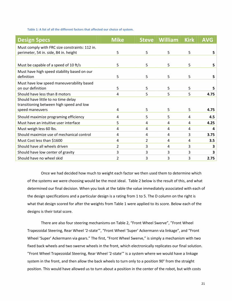
Table 1: A list of all the different factors that affected our choice of system.

Design Specs Mike Steve William Kirk AVG Must comply with FRC size constraints: 112 in. perimeter, 54 in. side, 84 in. height 5 5 5 5 5

Must be capable of a speed of 10 ft/s 5 5 5 5 5

Must have high speed stability based on our definition 5 5 5 5 5

Must have low speed maneuverability based on our definition 5 5 5 5 5

Should have less than 8 motors 4 5 5 5 4.75

Should have little to no time delay transitioning between high speed and low speed maneuvers 4 5 5 5 4.75

Should maximize programing efficiency 4 5 5 4 4.5

Must have an intuitive user interface 5 4 4 4 4.25

Must weigh less 60 lbs. 4 4 4 4 4

Should maximize use of mechanical control 4 4 4 3 3.75

Must Cost less than $1600 4 2 4 4 3.5

Should have all wheels driven 2 3 4 3 3

Should have low center of gravity 3 3 3 3 3

Should have no wheel skid 2 3 3 3 2.75

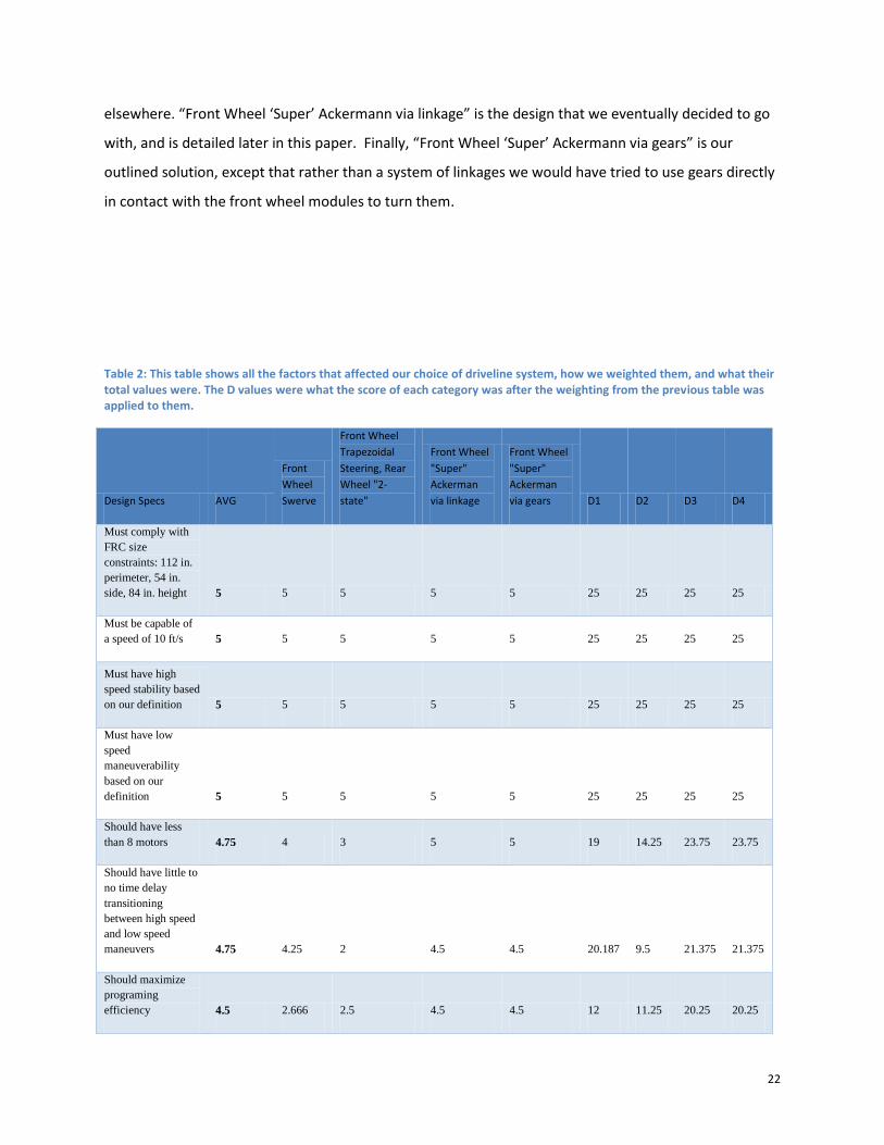
Once we had decided how much to weight each factor we then used them to determine which

of the systems we were choosing would be the most ideal. Table 2 below is the result of this, and what

determined our final decision. When you look at the table the value immediately associated with each of

the design specifications and a particular design is a rating from 1 to 5. The D column on the right is

what that design scored for after the weights from Table 1 were applied to its score. Below each of the

designs is their total score.

There are also four steering mechanisms on Table 2, “Front Wheel Swerve”, ”Front Wheel

Trapezoidal Steering, Rear Wheel ‘2-state’”, “Front Wheel ‘Super’ Ackermann via linkage”, and “Front

Wheel ‘Super’ Ackermann via gears.” The first, “Front Wheel Swerve,” is simply a mechanism with two

fixed back wheels and two swerve wheels in the front, which electronically replicates our final solution.

”Front Wheel Trapezoidal Steering, Rear Wheel ‘2-state’” is a system where we would have a linkage

system in the front, and then allow the back wheels to turn only to a position 90° from the straight

position. This would have allowed us to turn about a position in the center of the robot, but with costs

22

elsewhere. “Front Wheel ‘Super’ Ackermann via linkage” is the design that we eventually decided to go

with, and is detailed later in this paper. Finally, “Front Wheel ‘Super’ Ackermann via gears” is our

outlined solution, except that rather than a system of linkages we would have tried to use gears directly

in contact with the front wheel modules to turn them.

Table 2: This table shows all the factors that affected our choice of driveline system, how we weighted them, and what their total values were. The D values were what the score of each category was after the weighting from the previous table was applied to them.

Design Specs AVG

Front

Wheel

Swerve

Front Wheel

Trapezoidal

Steering, Rear

Wheel "2-

state"

Front Wheel

"Super"

Ackerman

via linkage

Front Wheel

"Super"

Ackerman

via gears D1 D2 D3 D4

Must comply with

FRC size

constraints: 112 in.

perimeter, 54 in.

side, 84 in. height 5 5 5 5 5 25 25 25 25

Must be capable of

a speed of 10 ft/s 5 5 5 5 5 25 25 25 25

Must have high

speed stability based

on our definition 5 5 5 5 5 25 25 25 25

Must have low

speed

maneuverability

based on our

definition 5 5 5 5 5 25 25 25 25

Should have less

than 8 motors 4.75 4 3 5 5 19 14.25 23.75 23.75

Should have little to

no time delay

transitioning

between high speed

and low speed

maneuvers 4.75 4.25 2 4.5 4.5 20.187 9.5 21.375 21.375

Should maximize

programing

efficiency 4.5 2.666 2.5 4.5 4.5 12 11.25 20.25 20.25

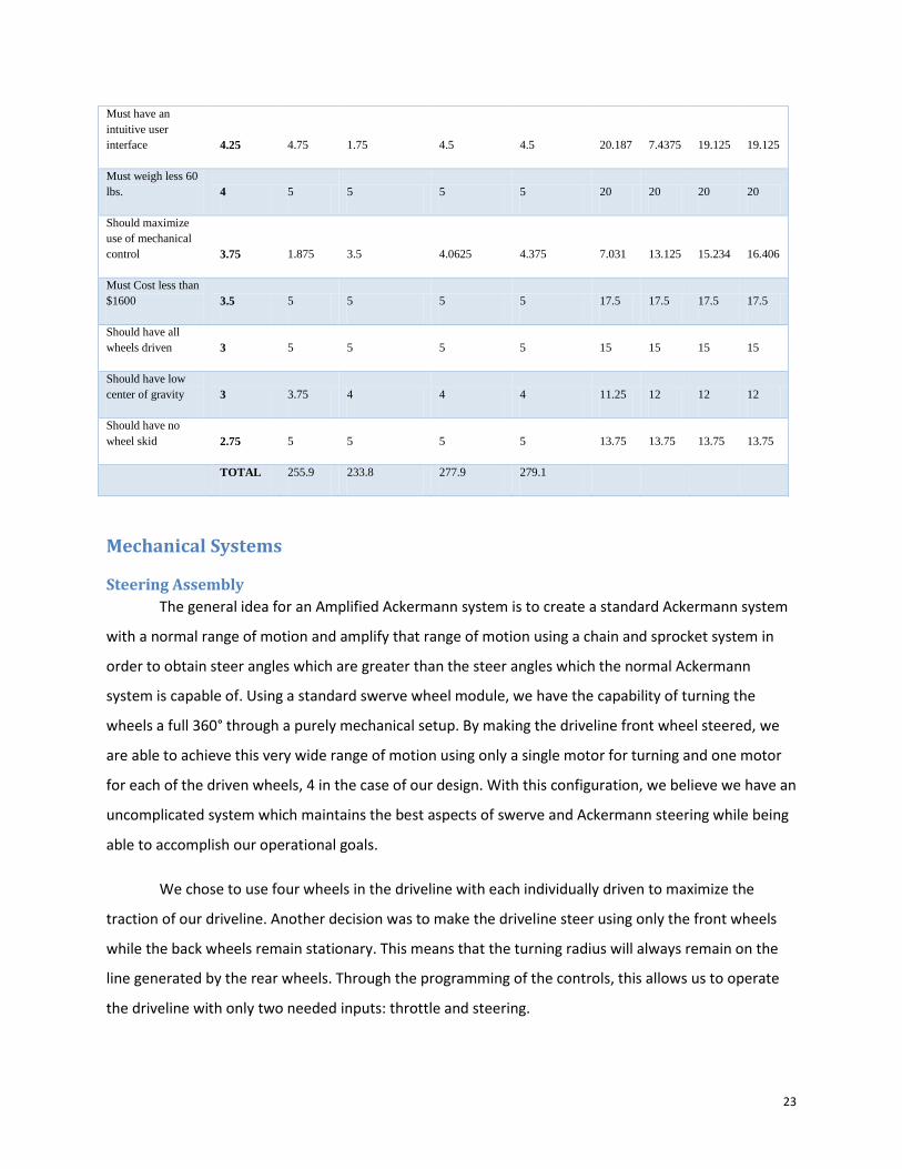
23

Must have an

intuitive user

interface 4.25 4.75 1.75 4.5 4.5 20.187 7.4375 19.125 19.125

Must weigh less 60

lbs. 4 5 5 5 5 20 20 20 20

Should maximize

use of mechanical

control 3.75 1.875 3.5 4.0625 4.375 7.031 13.125 15.234 16.406

Must Cost less than

$1600 3.5 5 5 5 5 17.5 17.5 17.5 17.5

Should have all

wheels driven 3 5 5 5 5 15 15 15 15

Should have low

center of gravity 3 3.75 4 4 4 11.25 12 12 12

Should have no

wheel skid 2.75 5 5 5 5 13.75 13.75 13.75 13.75

TOTAL 255.9 233.8 277.9 279.1

Mechanical Systems

Steering Assembly

The general idea for an Amplified Ackermann system is to create a standard Ackermann system

with a normal range of motion and amplify that range of motion using a chain and sprocket system in

order to obtain steer angles which are greater than the steer angles which the normal Ackermann

system is capable of. Using a standard swerve wheel module, we have the capability of turning the

wheels a full 360° through a purely mechanical setup. By making the driveline front wheel steered, we

are able to achieve this very wide range of motion using only a single motor for turning and one motor

for each of the driven wheels, 4 in the case of our design. With this configuration, we believe we have an

uncomplicated system which maintains the best aspects of swerve and Ackermann steering while being

able to accomplish our operational goals.

We chose to use four wheels in the driveline with each individually driven to maximize the

traction of our driveline. Another decision was to make the driveline steer using only the front wheels

while the back wheels remain stationary. This means that the turning radius will always remain on the

line generated by the rear wheels. Through the programming of the controls, this allows us to operate

the driveline with only two needed inputs: throttle and steering.

24

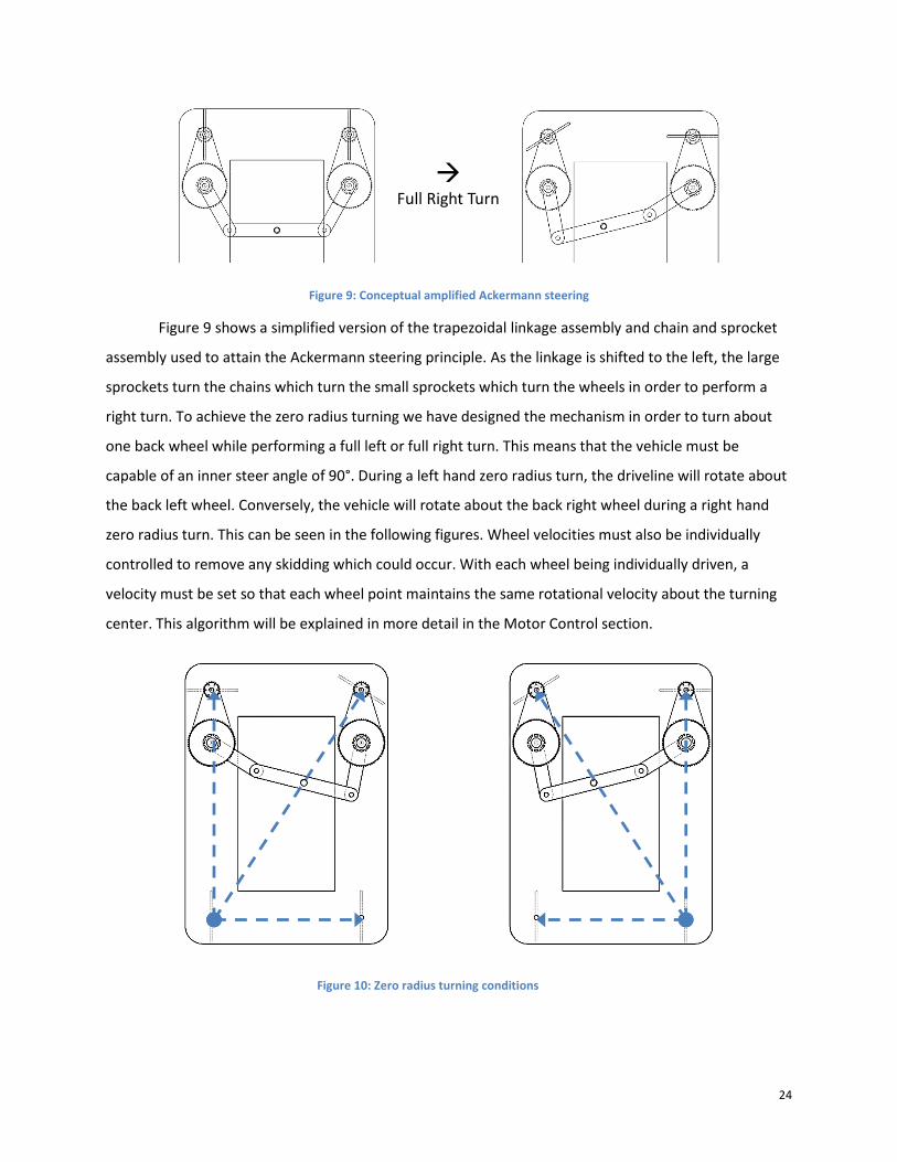
Figure 9: Conceptual amplified Ackermann steering

Figure 9 shows a simplified version of the trapezoidal linkage assembly and chain and sprocket

assembly used to attain the Ackermann steering principle. As the linkage is shifted to the left, the large

sprockets turn the chains which turn the small sprockets which turn the wheels in order to perform a

right turn. To achieve the zero radius turning we have designed the mechanism in order to turn about

one back wheel while performing a full left or full right turn. This means that the vehicle must be

capable of an inner steer angle of 90°. During a left hand zero radius turn, the driveline will rotate about

the back left wheel. Conversely, the vehicle will rotate about the back right wheel during a right hand

zero radius turn. This can be seen in the following figures. Wheel velocities must also be individually

controlled to remove any skidding which could occur. With each wheel being individually driven, a

velocity must be set so that each wheel point maintains the same rotational velocity about the turning

center. This algorithm will be explained in more detail in the Motor Control section.

Figure 10: Zero radius turning conditions

Full Right Turn

25

(2)

(3)

This operational decision was made because we feel it allows the driver of the vehicle to easily

orientate the driveline purely by seeing the motion of the vehicle. The driver can see if they are turning

full left or right based on the wheel about which the driveline is rotating. This also allows the driver to

visually see that driveline is moving in forward or reverse configuration even in zero turn radius

operation. With this setup, it also means that all wheels will be operating in the same direction at all

times except at zero radius where one wheel will be stopped. However, the linkage system can be

optimized so that the zero radius turning point is anywhere between the back wheels. This change will

also make the steer angle error slightly bigger in the middle ranges.

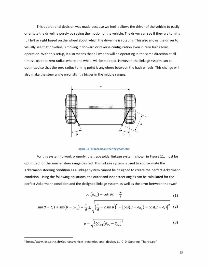
Figure 11: Trapezoidal steering geometry

For this system to work properly, the trapezoidal linkage system, shown in Figure 11, must be

optimized for the smaller steer range desired. This linkage system is used to approximate the

Ackermann steering condition as a linkage system cannot be designed to create the perfect Ackermann

condition. Using the following equations, the outer and inner steer angles can be calculated for the

perfect Ackermann condition and the designed linkage system as well as the error between the two:1

cot(𝛿𝐴𝑜) − cot(𝛿𝑖) =

𝑤

𝑙

sin(𝛽 + 𝛿𝑖) + sin(𝛽 − 𝛿𝐷𝑜) =

𝑤

𝑑± √(

𝑤

𝑑− 2 sin 𝛽)

2

− [cos(𝛽 − 𝛿𝐷𝑜) − cos(𝛽 + 𝛿𝑖)]

2

𝑒 = √1

𝑛∑ (𝛿𝐷𝑜

− 𝛿𝐴𝑜)

2𝑛𝑖=1

1 http://www.idsc.ethz.ch/Courses/vehicle_dynamics_and_design/11_0_0_Steering_Theroy.pdf

(1)

26

Equation 1 presents the condition for the perfect Ackerman system. δAo represents the

Ackermann outer steer angle while δi represents the inner steer angle. The second equation is for the

design of the trapezoidal geometry where δDo is the designed outer steer angle which is generally slightly

different than the perfect Ackermann condition. β is the angle at which the linkage bars connect to the

tie rod as shown in Figure 11. For both equations, the outer steer angle is calculated over a range of

inner steer angles. For n values of δi we can then find the error for a specific β in the trapezoidal

geometry. For all equations, w, l, and d represent the wheel track, wheelbase, and linkage length

respectively.

For our specific design, we must keep in mind that the steering angles are being amplified by the

chain system. We have designed the system with a gear ratio of 3:1 using VEXpro #25 sprockets of 66

teeth and 22 teeth. With this ratio we must then design the trapezoidal geometry to be effective for an

inner steer angle up to 30°, a third of the amplified 90° steer angle. For the calculations we have also

chosen the following values for the design: w = 17 in, l = 26 in, and d = 6 in. There are many different

ways the β value can be optimized and one would be to choose a value which would result in the lowest

error. However, because we want to be sure we have the zero turn radius established about the back

wheel, we calculate β from Equation 2 assuming δDo = δAo when the inner steer angle is 30°. This way we

can assure that the linkage system is perfect at 3 conditions: straight, full left, and full right. We find that

β = 29.246° and calculate the tie rod length to be 11.137 in. With this β value established we can then

calculate the error for the amplified system from the equations. Figure 12 shows a graph which

compares the amplified system we have created to the perfect Ackermann condition over the same

range of inner steer angles. It must also be noted that all steer angles must be multiplied by 3 due to the

amplification process.

27

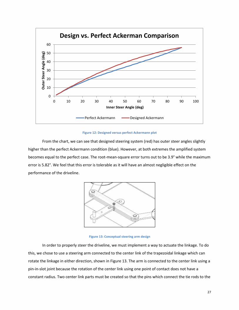
Figure 12: Designed versus perfect Ackermann plot

From the chart, we can see that designed steering system (red) has outer steer angles slightly

higher than the perfect Ackermann condition (blue). However, at both extremes the amplified system

becomes equal to the perfect case. The root-mean-square error turns out to be 3.9° while the maximum

error is 5.82°. We feel that this error is tolerable as it will have an almost negligible effect on the

performance of the driveline.

Figure 13: Conceptual steering arm design

In order to properly steer the driveline, we must implement a way to actuate the linkage. To do

this, we chose to use a steering arm connected to the center link of the trapezoidal linkage which can

rotate the linkage in either direction, shown in Figure 13. The arm is connected to the center link using a

pin-in-slot joint because the rotation of the center link using one point of contact does not have a

constant radius. Two center link parts must be created so that the pins which connect the tie rods to the

0

10

20

30

40

50

60

0 10 20 30 40 50 60 70 80 90 100

Ou

ter

Ste

er

An

gle

(d

eg)

Inner Steer Angle (deg)

Design vs. Perfect Ackerman Comparison

Perfect Ackermann Designed Ackermann

28

center link and the pin for the pin-in-slot joint can be supported in double shear and allow for even

distribution of forces. Due to the nature of the geometry, the force needed to actuate the linkage is not

linear and a much higher force is needed to rotate the arm at the limits of the steering range. Therefore,

a high-torque motor is needed to control the steering arm and this will be explained in greater detail in

the Motor Selection section.

Figure 14: Steering arm range of motion

The linkage system, the 3:1 ratio chain and sprocket system, and the steering arm make up the

steering assembly which will allow our driveline to be capable of the desired high and low speed

performance.

We determined the coefficient of friction and the weight requirement for our robot, by

assuming worst case scenarios. For rubber on carpet we were able to determine that this coefficient

would be .65 and we assumed 120lbs of force would be applied directly to each wheel, so that our

requirement would be a worst case scenario. We then converted the force to Newtons and multiplied

the friction force of .65 which allows us to find the minimum wheel shaft torque needed by assuming

the wheels are one inch thick. The minimum torque requirement, neglecting friction in the linkage

system, is 4.4 Nm. With the 3:1 amplification ratio we can then find the required torque for the linkage

shaft. Assuming that the steering arm maintains a 90 degree angle to the center link, we can then find

necessary force applied and resultant torque of the steering arm shaft. For good performance, we

decided that the linkage system would need to cover the full range of steer angles in one second. To do

this, the shaft’s rotational speed would need to be 7.5 RPM. With the rotational speed and shaft torque

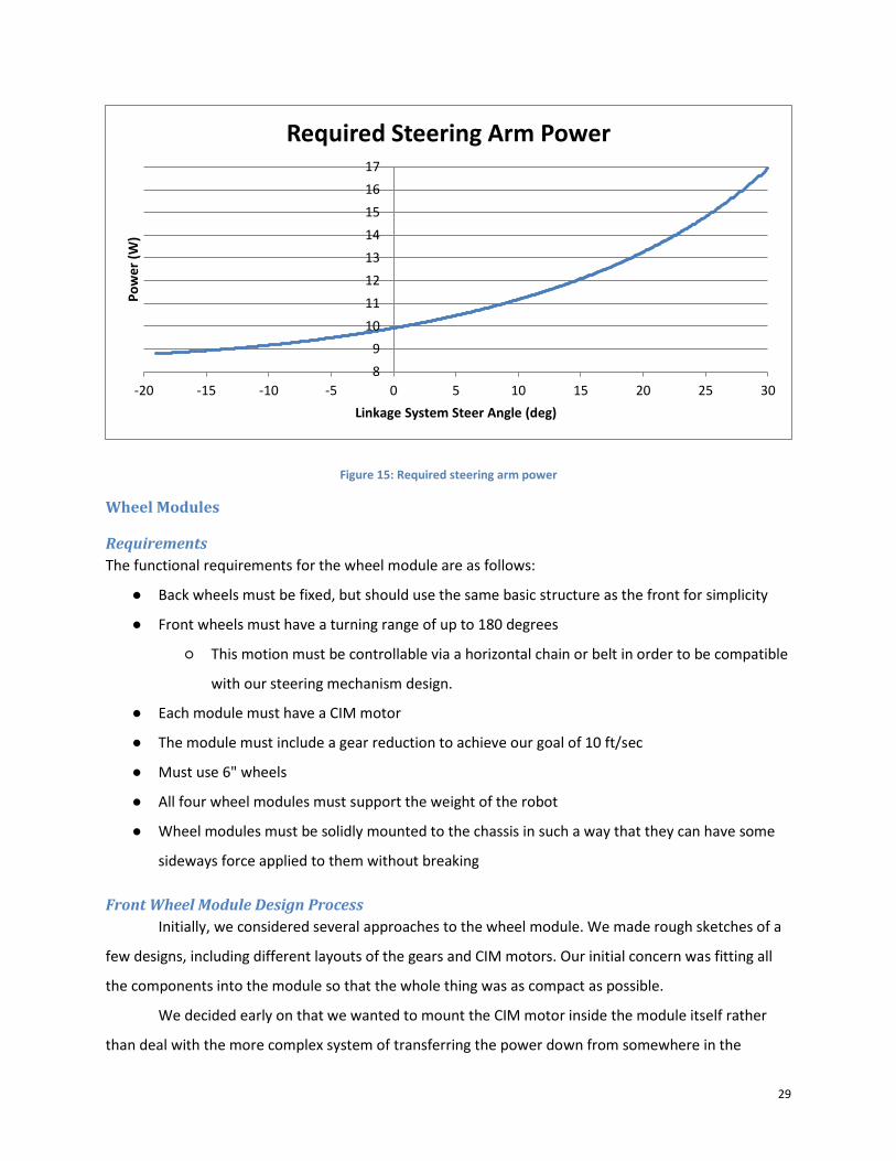
known, we can find the power needed over the range of steer angles. Figure 15 shows this relationship

over the steer angle range of the linkage system where a negative angle indicates an outer steer angle

and a positive indicates an inner steer angle. From this we determined that the maximum power needed

would be 16.92 W. These calculations can be seen in the Appendix.

29

Figure 15: Required steering arm power

Wheel Modules

Requirements

The functional requirements for the wheel module are as follows:

● Back wheels must be fixed, but should use the same basic structure as the front for simplicity

● Front wheels must have a turning range of up to 180 degrees

○ This motion must be controllable via a horizontal chain or belt in order to be compatible

with our steering mechanism design.

● Each module must have a CIM motor

● The module must include a gear reduction to achieve our goal of 10 ft/sec

● Must use 6" wheels

● All four wheel modules must support the weight of the robot

● Wheel modules must be solidly mounted to the chassis in such a way that they can have some

sideways force applied to them without breaking

Front Wheel Module Design Process

Initially, we considered several approaches to the wheel module. We made rough sketches of a

few designs, including different layouts of the gears and CIM motors. Our initial concern was fitting all

the components into the module so that the whole thing was as compact as possible.

We decided early on that we wanted to mount the CIM motor inside the module itself rather

than deal with the more complex system of transferring the power down from somewhere in the

8

9

10

11

12

13

14

15

16

17

-20 -15 -10 -5 0 5 10 15 20 25 30

Po

we

r (W

)

Linkage System Steer Angle (deg)

Required Steering Arm Power

30

chassis. This decision avoids a significant amount of gearing, and simplifies the design. Treating the

wheel module as a standalone unit (with CIM included), we also needed a way to rotate it via a chain

from the steering mechanism. We decided that the best way to do this was to attach a sprocket

horizontally at the top of the module. The module would then be mounted to the chassis above that

sprocket, using bearings and some sort of vertical shaft.

The next step was to design a gearbox capable of producing the required RPM at the wheel.

Since the maximum power of a CIM is delivered when the motor runs at 50% of its free-running speed,

we did our calculations based on the moor speed of 2650 RPM. We geared this down so that with 6”

wheels (which have a circumference of 18.85”) the robot would run at 10ft/s. It is important to note that

the robot may be capable of going faster than this, but the maximum power will be delivered at a

velocity of 10ft/s. As discussed in the Motor Selection section, we determined that the gear ratio should

be 6.95:1. Using this desired gear ratio, we began looking for gears that would achieve this in a two-

stage reduction. Initially, we wanted to use one spur gear stage and one chain and sprocket stage.

However, we learned that this would require the final small sprocket to have 9 teeth, which is too few.

So we decided to go with a three stage reduction of spur gears instead. After discovering that the spur

gears we wanted were very expensive, we began to look into off-the-shelf wheel module kits that

included gears.

This research opened up new options for the wheel module design. We had already settled on

several specifications, and we were able to find wheel module kits that closely resembled what we were

planning to build ourselves. The most intriguing was the AndyMark Wild Swerve Module. This module

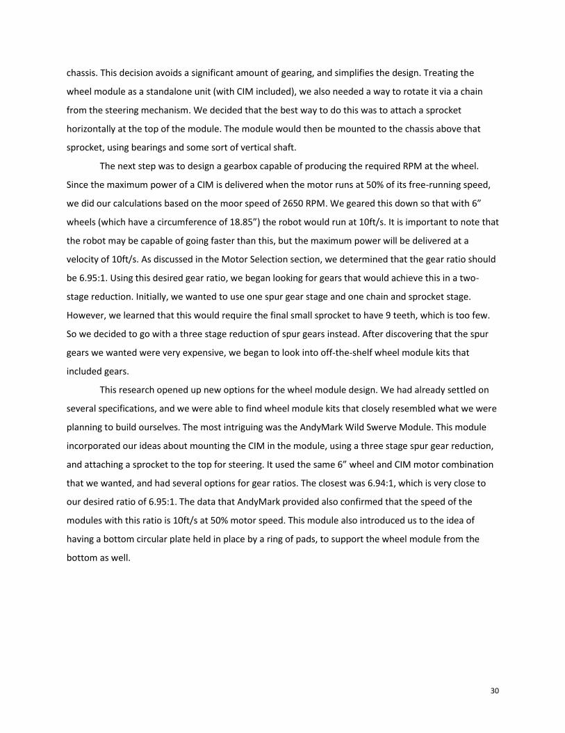
incorporated our ideas about mounting the CIM in the module, using a three stage spur gear reduction,

and attaching a sprocket to the top for steering. It used the same 6” wheel and CIM motor combination

that we wanted, and had several options for gear ratios. The closest was 6.94:1, which is very close to

our desired ratio of 6.95:1. The data that AndyMark provided also confirmed that the speed of the

modules with this ratio is 10ft/s at 50% motor speed. This module also introduced us to the idea of

having a bottom circular plate held in place by a ring of pads, to support the wheel module from the

bottom as well.

31

Figure 16: AndyMark Wild Swerve Drive Module

Even though our intention was never to use a swerve drive system, the swerve module is

actually compatible with our ideas as well. The key feature of swerve drive is the ability to rotate the

entire wheel module via a sprocket at the top. While we were not planning to rotate each wheel

independently or link them together the way swerve systems sometimes do, we could still use the

sprocket to connect the swerve module to our own modified Ackermann steering mechanism.

Since the cost of the AndyMark module was comparable to what we would have spent building

our own, we decided to use these instead to save time. We began by downloading the CAD model from

AndyMark and disassembling it to gain an understanding of how it worked. We looked into making our

own parts to mimic this design, but ultimately decided that we could not build it for significantly cheaper

than the off-the-shelf version.

Our focus then shifted to modifying the Wild Swerve module to suite our needs. We had already

begun to design a chassis with two horizontal plates that could easily be mounted to the top and bottom

support plates of the Wild Swerve module. Aside from mounting the module to the chassis, the other

concern was integrating the module into our steering mechanism design. We had already decided that

we needed a 3:1 reduction from the Ackermann system to the wheel module. The Wild Swerve module

comes with a 36 tooth sprocket for steering. This would have required us to use a 108 tooth sprocket at

the other end. Since this was not feasible, we concluded that we would have to replace the module’s

sprocket with a smaller one.

32

Figure 17: Original bracket assembly

Figure 18: Modified bracket assembly

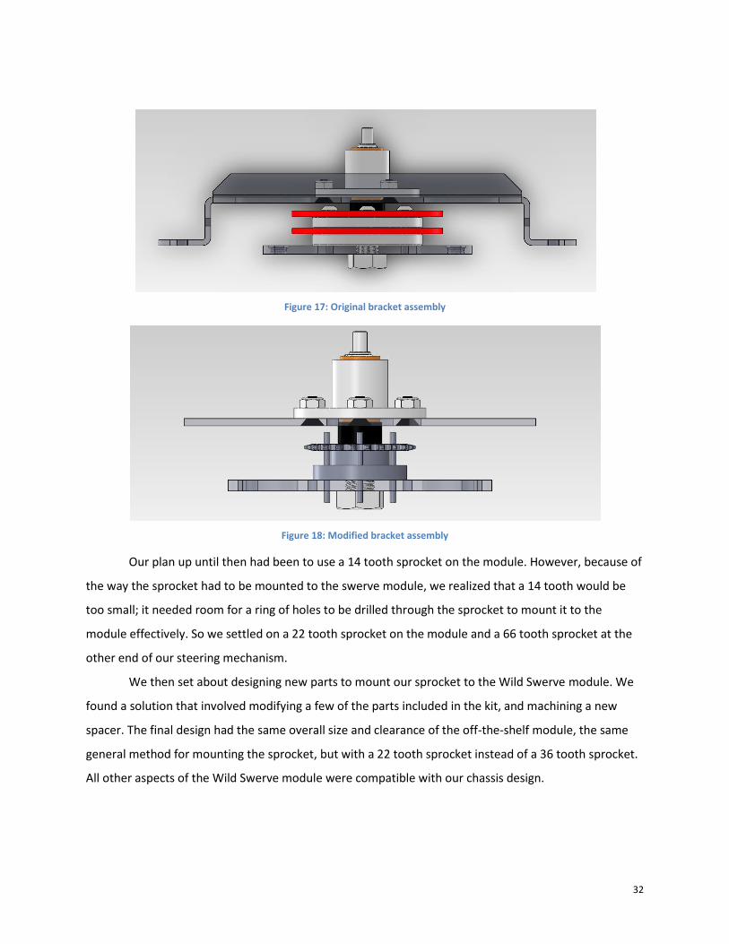
Our plan up until then had been to use a 14 tooth sprocket on the module. However, because of

the way the sprocket had to be mounted to the swerve module, we realized that a 14 tooth would be

too small; it needed room for a ring of holes to be drilled through the sprocket to mount it to the

module effectively. So we settled on a 22 tooth sprocket on the module and a 66 tooth sprocket at the

other end of our steering mechanism.

We then set about designing new parts to mount our sprocket to the Wild Swerve module. We

found a solution that involved modifying a few of the parts included in the kit, and machining a new

spacer. The final design had the same overall size and clearance of the off-the-shelf module, the same

general method for mounting the sprocket, but with a 22 tooth sprocket instead of a 36 tooth sprocket.

All other aspects of the Wild Swerve module were compatible with our chassis design.

33

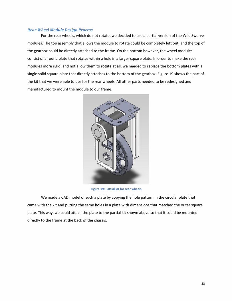
Rear Wheel Module Design Process

For the rear wheels, which do not rotate, we decided to use a partial version of the Wild Swerve

modules. The top assembly that allows the module to rotate could be completely left out, and the top of

the gearbox could be directly attached to the frame. On the bottom however, the wheel modules

consist of a round plate that rotates within a hole in a larger square plate. In order to make the rear

modules more rigid, and not allow them to rotate at all, we needed to replace the bottom plates with a

single solid square plate that directly attaches to the bottom of the gearbox. Figure 19 shows the part of

the kit that we were able to use for the rear wheels. All other parts needed to be redesigned and

manufactured to mount the module to our frame.

Figure 19: Partial kit for rear wheels

We made a CAD model of such a plate by copying the hole pattern in the circular plate that

came with the kit and putting the same holes in a plate with dimensions that matched the outer square

plate. This way, we could attach the plate to the partial kit shown above so that it could be mounted

directly to the frame at the back of the chassis.

34

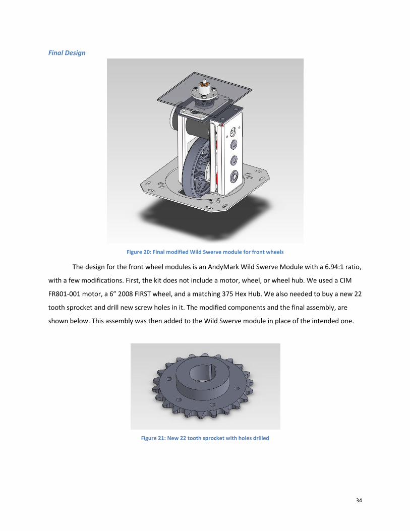
Final Design

Figure 20: Final modified Wild Swerve module for front wheels

The design for the front wheel modules is an AndyMark Wild Swerve Module with a 6.94:1 ratio,

with a few modifications. First, the kit does not include a motor, wheel, or wheel hub. We used a CIM

FR801-001 motor, a 6” 2008 FIRST wheel, and a matching 375 Hex Hub. We also needed to buy a new 22

tooth sprocket and drill new screw holes in it. The modified components and the final assembly, are

shown below. This assembly was then added to the Wild Swerve module in place of the intended one.

Figure 21: New 22 tooth sprocket with holes drilled

35

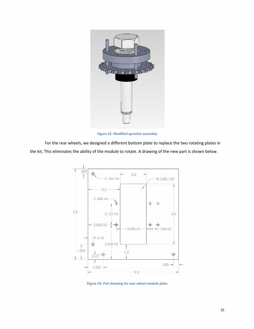
Figure 22: Modified sprocket assembly

For the rear wheels, we designed a different bottom plate to replace the two rotating plates in

the kit. This eliminates the ability of the module to rotate. A drawing of the new part is shown below.

Figure 23: Part drawing for rear wheel module plate

36

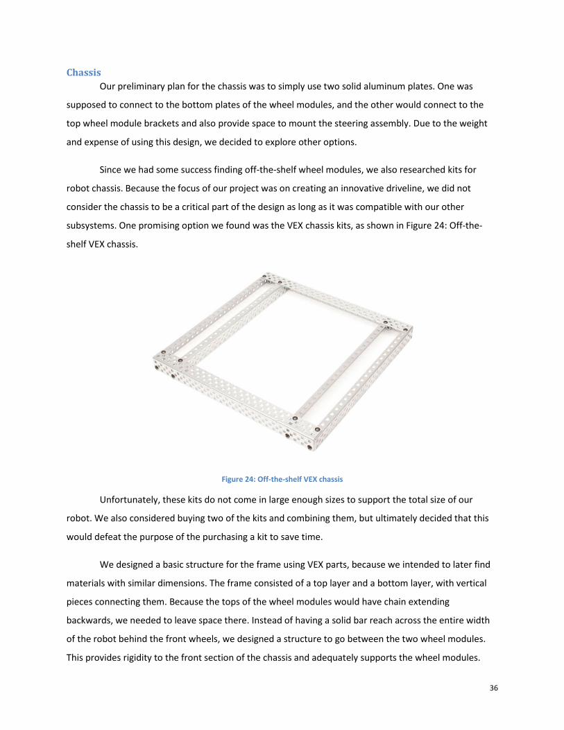
Chassis

Our preliminary plan for the chassis was to simply use two solid aluminum plates. One was

supposed to connect to the bottom plates of the wheel modules, and the other would connect to the

top wheel module brackets and also provide space to mount the steering assembly. Due to the weight

and expense of using this design, we decided to explore other options.

Since we had some success finding off-the-shelf wheel modules, we also researched kits for

robot chassis. Because the focus of our project was on creating an innovative driveline, we did not

consider the chassis to be a critical part of the design as long as it was compatible with our other

subsystems. One promising option we found was the VEX chassis kits, as shown in Figure 24: Off-the-

shelf VEX chassis.

Figure 24: Off-the-shelf VEX chassis

Unfortunately, these kits do not come in large enough sizes to support the total size of our

robot. We also considered buying two of the kits and combining them, but ultimately decided that this

would defeat the purpose of the purchasing a kit to save time.

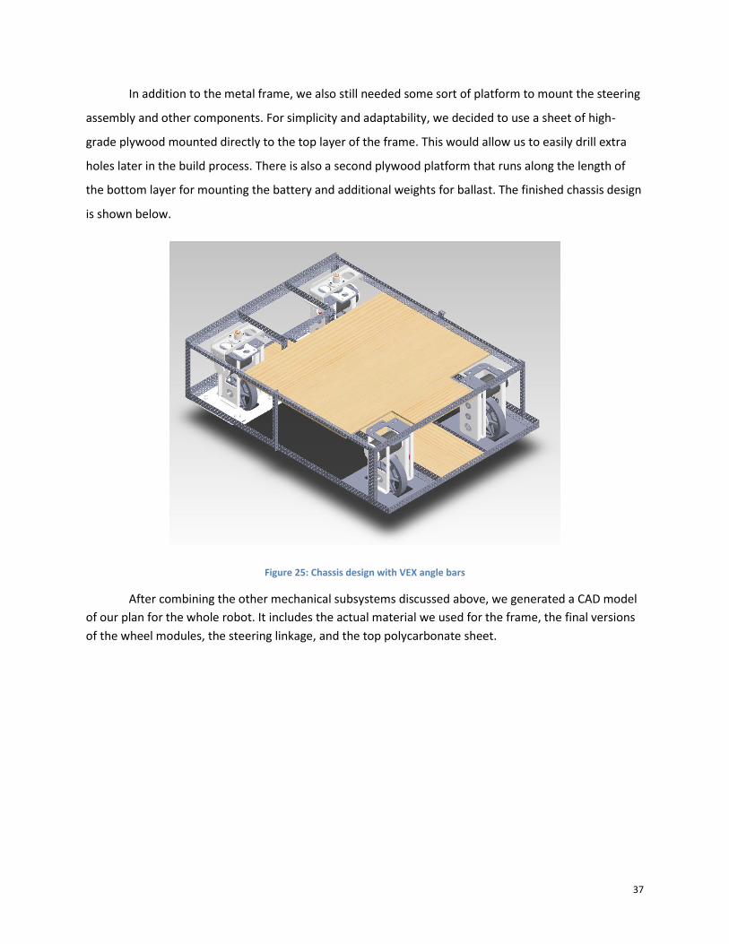
We designed a basic structure for the frame using VEX parts, because we intended to later find

materials with similar dimensions. The frame consisted of a top layer and a bottom layer, with vertical

pieces connecting them. Because the tops of the wheel modules would have chain extending

backwards, we needed to leave space there. Instead of having a solid bar reach across the entire width

of the robot behind the front wheels, we designed a structure to go between the two wheel modules.

This provides rigidity to the front section of the chassis and adequately supports the wheel modules.

37

In addition to the metal frame, we also still needed some sort of platform to mount the steering

assembly and other components. For simplicity and adaptability, we decided to use a sheet of high-

grade plywood mounted directly to the top layer of the frame. This would allow us to easily drill extra

holes later in the build process. There is also a second plywood platform that runs along the length of

the bottom layer for mounting the battery and additional weights for ballast. The finished chassis design

is shown below.

Figure 25: Chassis design with VEX angle bars

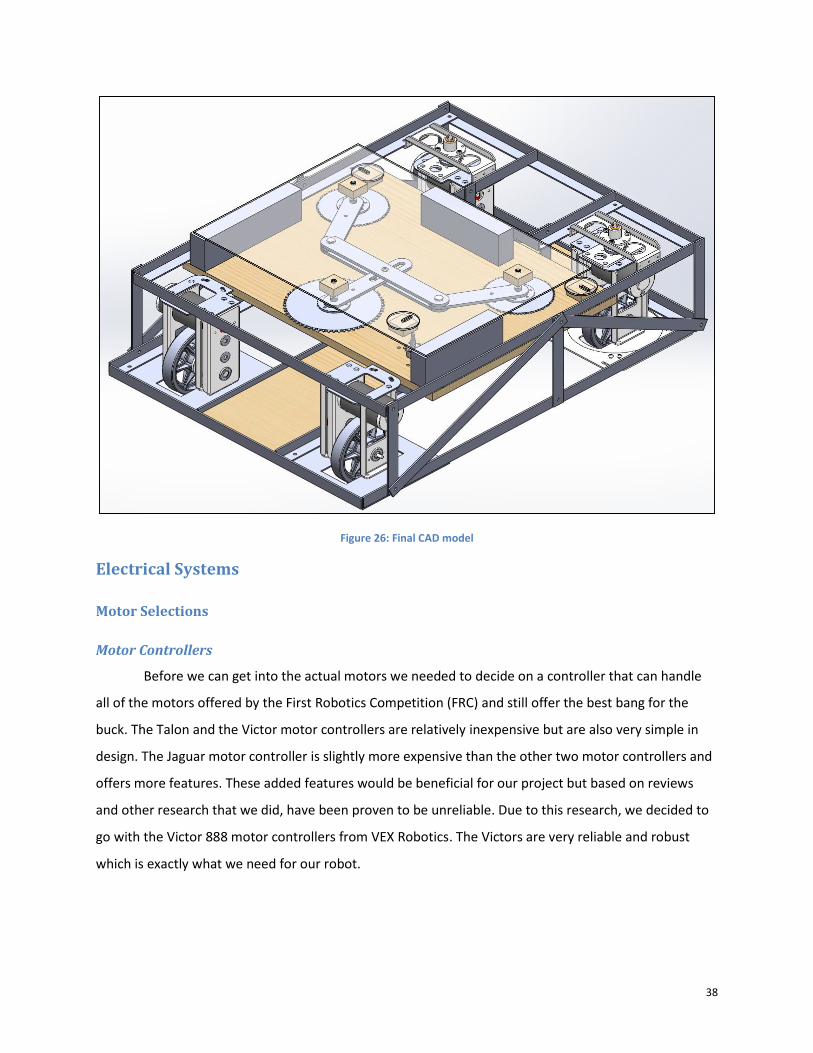
After combining the other mechanical subsystems discussed above, we generated a CAD model

of our plan for the whole robot. It includes the actual material we used for the frame, the final versions

of the wheel modules, the steering linkage, and the top polycarbonate sheet.

38

Figure 26: Final CAD model

Electrical Systems

Motor Selections

Motor Controllers

Before we can get into the actual motors we needed to decide on a controller that can handle

all of the motors offered by the First Robotics Competition (FRC) and still offer the best bang for the

buck. The Talon and the Victor motor controllers are relatively inexpensive but are also very simple in

design. The Jaguar motor controller is slightly more expensive than the other two motor controllers and

offers more features. These added features would be beneficial for our project but based on reviews

and other research that we did, have been proven to be unreliable. Due to this research, we decided to

go with the Victor 888 motor controllers from VEX Robotics. The Victors are very reliable and robust

which is exactly what we need for our robot.

39

Driving Motors

The first motor we looked at to drive our chassis was the CIM FR801-001 motor, since it was

readily available to us and the robot we would eventually test against would be powered by them as

well. For the high speed stability portion of our project, our robot needs to be able to go at least 10ft/s.

This motor coupled with the “Wild Swerve” wheel module from AndyMark with the Gear Ratio of 6.94:1

allows the us to produce a speed of 10.4 ft/s which is above the desired of 10 ft/s. The maximum power

will be delivered at a velocity of 10ft/s when the motor is running at 50% of its free spin speed.

Turning Motor

Based on our previous calculations of the power required of the turning motor, we knew that

we would need at least 16.92W. There were two options that were readily available to us: the Bosch

Van Door motor with 53W and the Snow blower from AndyMark with 30W. With the correct gearing,

either of these were a viable option. We chose to investigate the Van Door motor first because of its

higher power.

We were able to confirm that this motor would perform well by working backwards through the

same process that we used to determine the power requirements. We had also already determined that

we would have to use a gear ration of 6:1 in order to achieve a speed of 7.5RPM at the base of the

steering arm. This is fast enough to drive our linkage rom full left to full right in 1 second. Based on this

gear ratio, we found the torque applied to the steering arm. By dividing by the lever arm, we calculated

the force applied to our trapezoidal linkage. This can then be used to find the torque applied to the

sprockets on the wheel modules with the assumption that the steering arm remains perpendicular to

the center link. The minimum torque generated in the wheel module shaft becomes 12.95 Nm which is

greater than necessary 4.4 Nm. However, these calculations ignore any friction in our linkage. The plot

below shows the torque in both the linkage shafts and the wheel module shafts over the entire steer

angle range of the linkage system. These calculations can be seen in the Appendix.

40

Figure 27: Van door motor output torque

Microcontroller

The Arduino Mega 2560 is the microcontroller that we have chosen for our design. We initially

started looking into Arduino microcontrollers as an alternative to the FIRST Robotics cRIO because of the

costs; there is approximately a $700 difference between the Arduino products and cRIO. Once we

started looking at the different Arduinos that were available to us we came to the conclusion that the

standard board, with only one set of transmit/receive pins and not very many digital ports could prove

to be a problem. For this reason we switched to the Arduino Mega 2560 which has multiple transmit and

receive ports as well as digital and analog ports. The extensive amount of ports will assist us in having

plenty of options and alternatives to choose from. Another major point is that Arduinos have extensive

open source libraries that we can take advantage of. This includes some tutorials on how to set them up

to run Victors, which will be extremely helpful when we begin the process of wiring and programming

our system.

Sensors

We are using several sensors in our design to ensure that we are able to properly control and

monitor the various systems, in order to meet the performance criteria we have laid out. For example, it

is critically important that we can tell how far our steering motor has turned our wheels to ensure it

does not lock up. In order to prevent this we have a potentiometer to measure how far from straight

ahead it has turned, with limit switches as a failsafe mounted to the chassis. The potentiometer will also

0

10

20

30

40

50

60

70

80

-20 -15 -10 -5 0 5 10 15 20 25 30

Torq

ue

(N

m)

Linkage System Steer Angle (deg)

Van Door Motor Output Torque

Linkage Shaft Torque

Wheel Shaft Torque

41

be able to tell us what degree of turn we are currently making which we can use in our wheel speed

algorithm.

The potentiometer we plan to use has a 300 degree range of accurate readings. This will be

mounted so that it is turned by our steering motor, and therefore will allow us to keep track of where it

is relative to our center, or straight, position. The turning motor we have determined will have to move

no more than 270 degrees, and as such the 300 we’re able to use with this sensor is more than enough.

This potentiometer in particular was chosen for its low price and the ease of acquisition.

Next is a VEX brand limit switch, this will be mounted on our chassis so that our steering

mechanism will hit it before it gets so far that it locks up. We will program the switch to prevent the

motor from turning any more in the direction that would cause lock up. The motor is allowed to turn

away from this point but no further in the limit switches direction if the switch has been activated. We

have selected this particular limit switch because of its low cost and ease of use.

Teleoperation

The controller that we have selected to use with our system is a Turnigy 9X 2.4Ghz 9 channel

transmitter and receiver with dual joysticks on each side. We will program a setting where the left hand

joystick, will control the throttle of the wheels and the right stick will be used for turning. Another nice

feature of this controller is that the sticks are self-centering, so we don’t have to worry about the driver

needing to center the steering and throttle manually. The biggest reason for choosing this controller was

because of how common these types of controllers are. This should make it easier for other people to

learn very quickly how the robot operates.

Schematic

Below is a basic diagram of the electrical schematic that was used to wire together all of our

components.

42

Figure 28: Electrical schematic

Programming

Motor Control

As mentioned earlier, we decided to go with Victor 888 motor controllers. The motor controllers

will be wired to the Arduino via 3 wires. These wires will be carrying signal, 5 Volts, and ground. The

Arduino will send the Victors signals based on the sensors and wheel speed algorithms. These signals

will be in the form of Servo values which the Victor will convert to Pulse Width Modulation (PWM)

signals.

The four CIM motors that will be used for the wheel modules will receive a signal from their

respective Victors based on the wheel speed algorithm. The algorithm will take in the throttle value

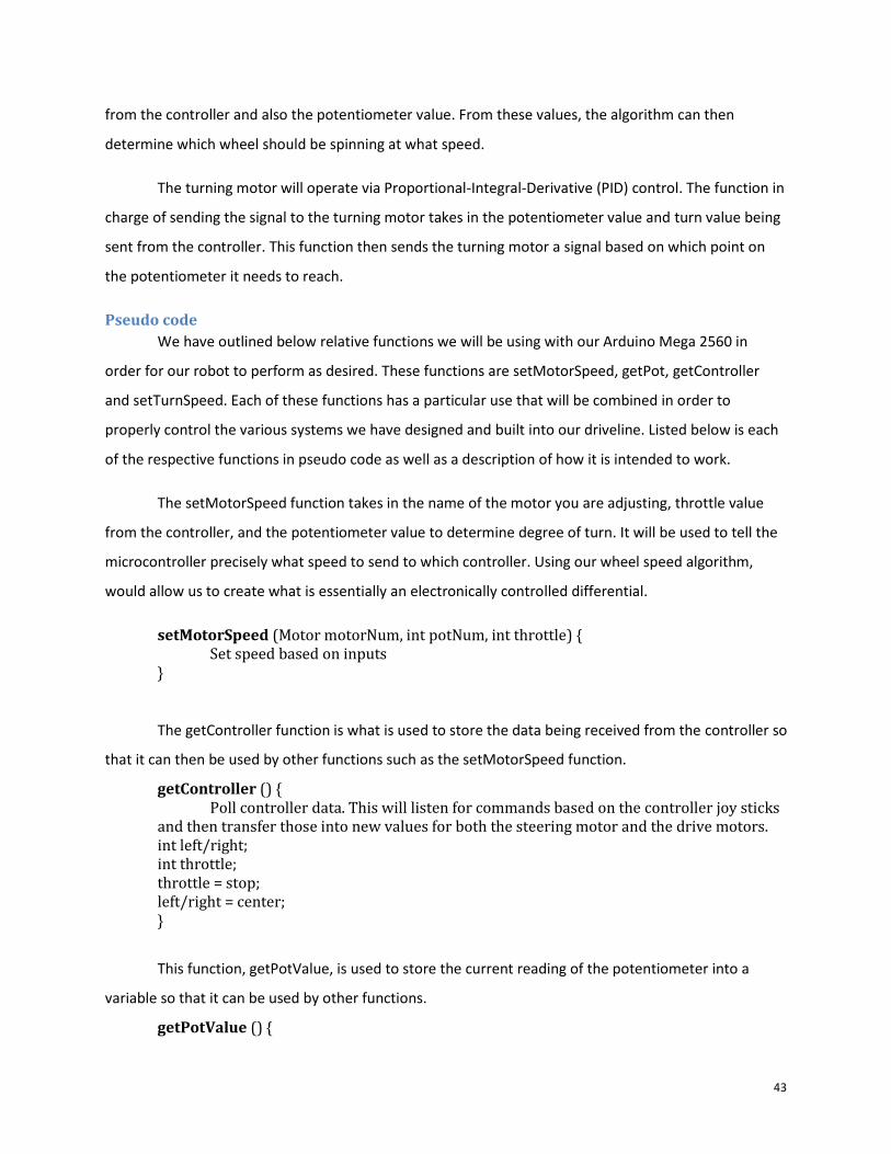
43

from the controller and also the potentiometer value. From these values, the algorithm can then

determine which wheel should be spinning at what speed.

The turning motor will operate via Proportional-Integral-Derivative (PID) control. The function in

charge of sending the signal to the turning motor takes in the potentiometer value and turn value being

sent from the controller. This function then sends the turning motor a signal based on which point on

the potentiometer it needs to reach.

Pseudo code

We have outlined below relative functions we will be using with our Arduino Mega 2560 in

order for our robot to perform as desired. These functions are setMotorSpeed, getPot, getController

and setTurnSpeed. Each of these functions has a particular use that will be combined in order to

properly control the various systems we have designed and built into our driveline. Listed below is each

of the respective functions in pseudo code as well as a description of how it is intended to work.

The setMotorSpeed function takes in the name of the motor you are adjusting, throttle value

from the controller, and the potentiometer value to determine degree of turn. It will be used to tell the

microcontroller precisely what speed to send to which controller. Using our wheel speed algorithm,

would allow us to create what is essentially an electronically controlled differential.

setMotorSpeed (Motor motorNum, int potNum, int throttle) { Set speed based on inputs }

The getController function is what is used to store the data being received from the controller so

that it can then be used by other functions such as the setMotorSpeed function.

getController () { Poll controller data. This will listen for commands based on the controller joy sticks and then transfer those into new values for both the steering motor and the drive motors. int left/right; int throttle; throttle = stop; left/right = center; }

This function, getPotValue, is used to store the current reading of the potentiometer into a

variable so that it can be used by other functions.

getPotValue () {

44

Poll pot data to be used to determine the location of the steering motor. Will store this in a global variable. int potPosition = potNum; }

The setTurnSpeed function will set the turning motor to a particular value based on the input

from the controller and potentiometer.

setTurnSpeed (int potNum, int left/right) { Turns linkage to desired location based on current value and joystick input. }

Budget Below is our budget for this project. The Arduino Mega 2560 and Turnigy 9x have costs of $0 because

they were previously acquired by one of the group members. Everything else that has $0 was loaned to

our group from the FRC 190 team or Robotics Engineering Department.

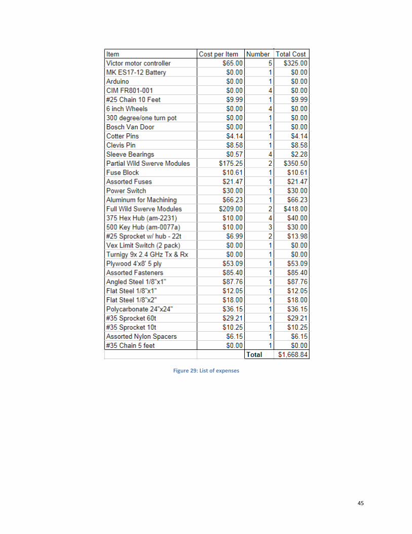
45

Figure 29: List of expenses

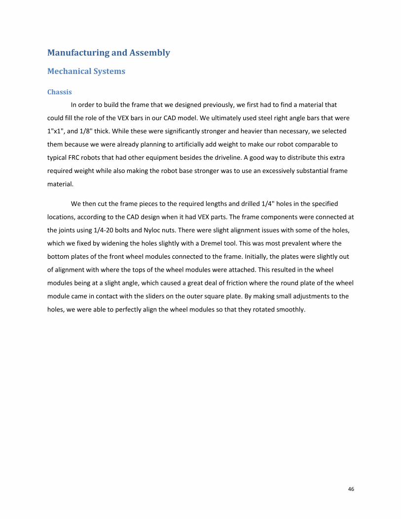
46

Manufacturing and Assembly

Mechanical Systems

Chassis

In order to build the frame that we designed previously, we first had to find a material that

could fill the role of the VEX bars in our CAD model. We ultimately used steel right angle bars that were

1"x1", and 1/8" thick. While these were significantly stronger and heavier than necessary, we selected

them because we were already planning to artificially add weight to make our robot comparable to

typical FRC robots that had other equipment besides the driveline. A good way to distribute this extra

required weight while also making the robot base stronger was to use an excessively substantial frame

material.

We then cut the frame pieces to the required lengths and drilled 1/4" holes in the specified

locations, according to the CAD design when it had VEX parts. The frame components were connected at

the joints using 1/4-20 bolts and Nyloc nuts. There were slight alignment issues with some of the holes,

which we fixed by widening the holes slightly with a Dremel tool. This was most prevalent where the

bottom plates of the front wheel modules connected to the frame. Initially, the plates were slightly out

of alignment with where the tops of the wheel modules were attached. This resulted in the wheel

modules being at a slight angle, which caused a great deal of friction where the round plate of the wheel

module came in contact with the sliders on the outer square plate. By making small adjustments to the

holes, we were able to perfectly align the wheel modules so that they rotated smoothly.

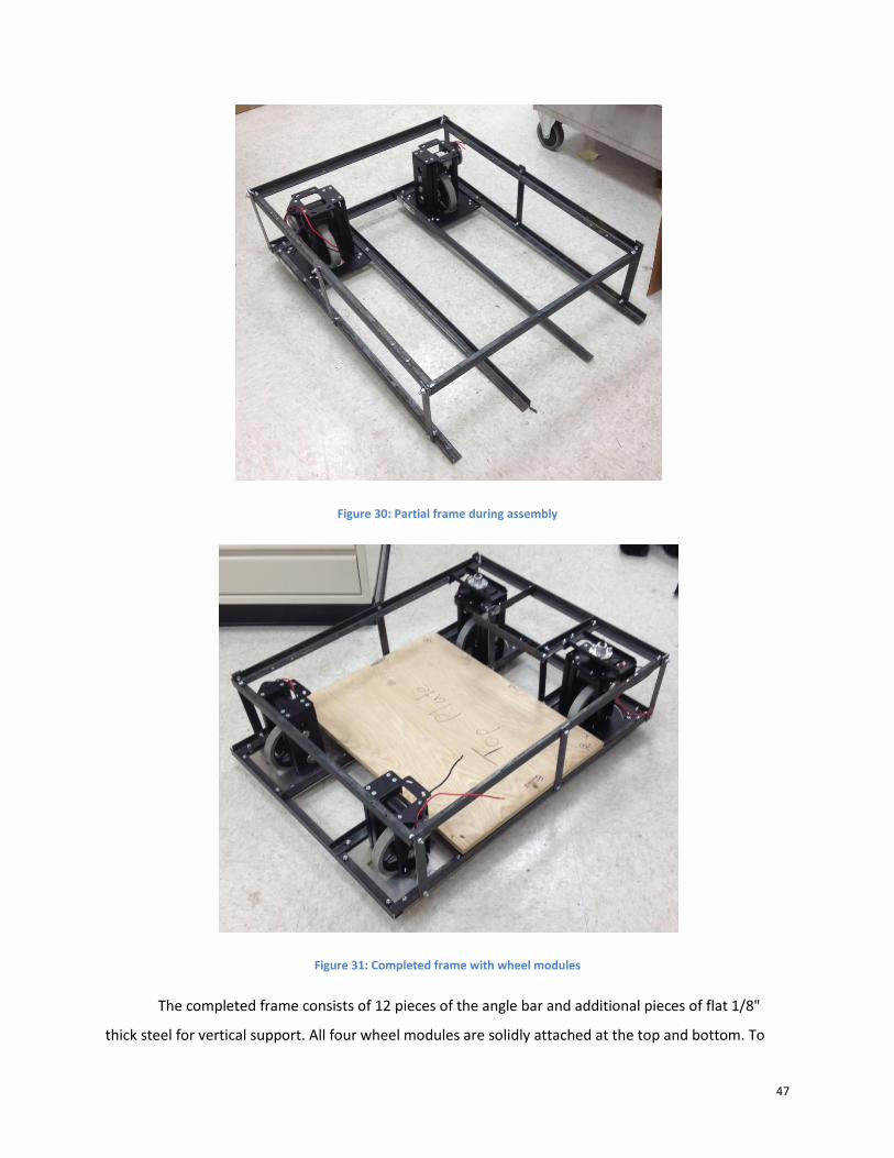
47

Figure 30: Partial frame during assembly

Figure 31: Completed frame with wheel modules

The completed frame consists of 12 pieces of the angle bar and additional pieces of flat 1/8"

thick steel for vertical support. All four wheel modules are solidly attached at the top and bottom. To

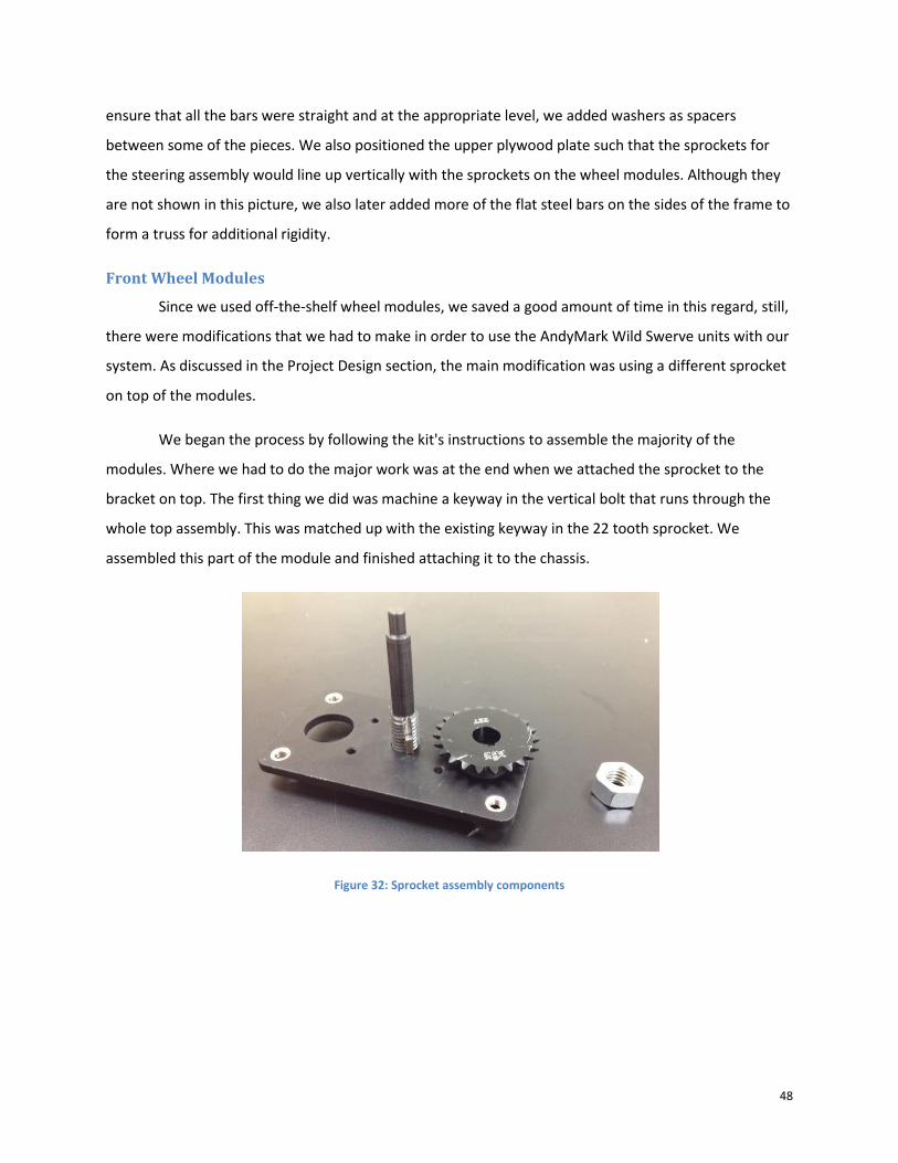
48

ensure that all the bars were straight and at the appropriate level, we added washers as spacers

between some of the pieces. We also positioned the upper plywood plate such that the sprockets for

the steering assembly would line up vertically with the sprockets on the wheel modules. Although they

are not shown in this picture, we also later added more of the flat steel bars on the sides of the frame to

form a truss for additional rigidity.

Front Wheel Modules

Since we used off-the-shelf wheel modules, we saved a good amount of time in this regard, still,

there were modifications that we had to make in order to use the AndyMark Wild Swerve units with our

system. As discussed in the Project Design section, the main modification was using a different sprocket

on top of the modules.

We began the process by following the kit's instructions to assemble the majority of the

modules. Where we had to do the major work was at the end when we attached the sprocket to the

bracket on top. The first thing we did was machine a keyway in the vertical bolt that runs through the

whole top assembly. This was matched up with the existing keyway in the 22 tooth sprocket. We

assembled this part of the module and finished attaching it to the chassis.

Figure 32: Sprocket assembly components

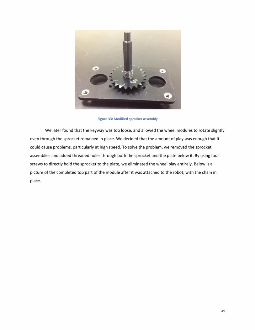
49

Figure 33: Modified sprocket assembly

We later found that the keyway was too loose, and allowed the wheel modules to rotate slightly

even through the sprocket remained in place. We decided that the amount of play was enough that it

could cause problems, particularly at high speed. To solve the problem, we removed the sprocket

assemblies and added threaded holes through both the sprocket and the plate below it. By using four

screws to directly hold the sprocket to the plate, we eliminated the wheel play entirely. Below is a

picture of the completed top part of the module after it was attached to the robot, with the chain in

place.

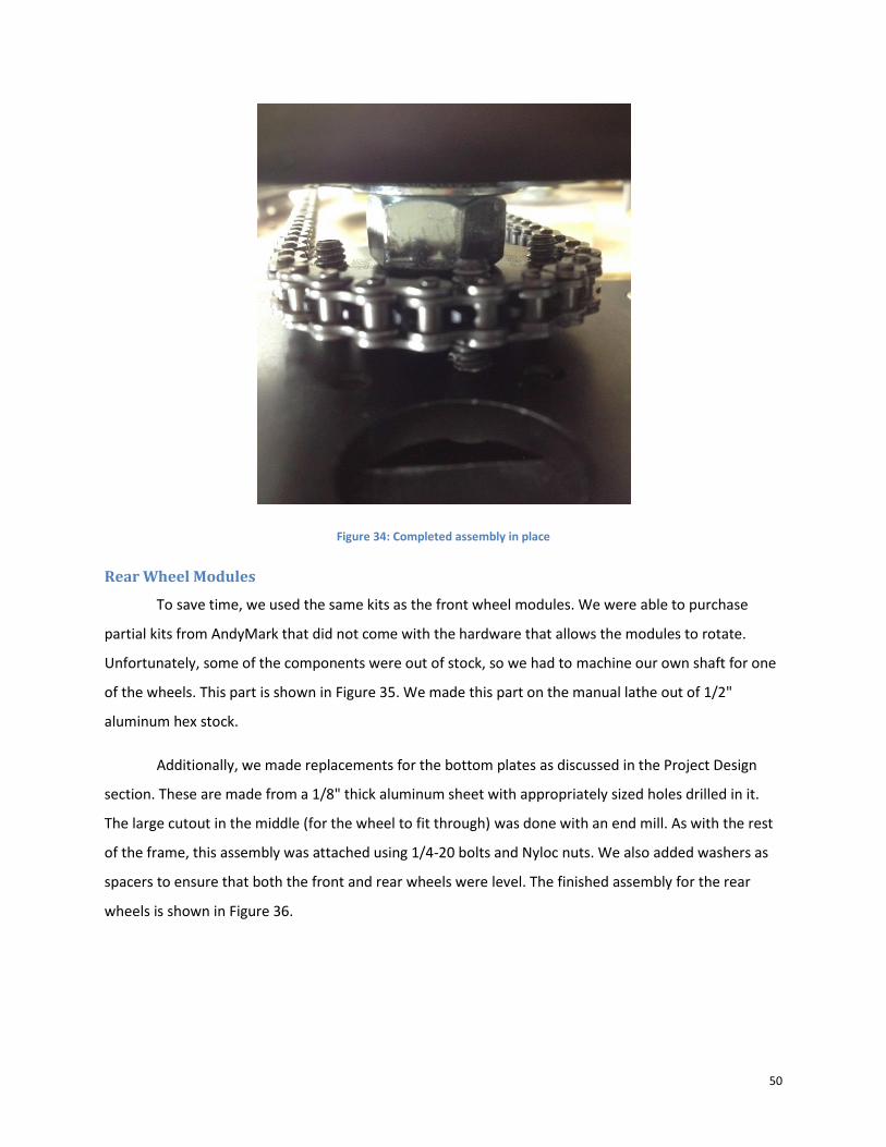
50

Figure 34: Completed assembly in place

Rear Wheel Modules

To save time, we used the same kits as the front wheel modules. We were able to purchase

partial kits from AndyMark that did not come with the hardware that allows the modules to rotate.

Unfortunately, some of the components were out of stock, so we had to machine our own shaft for one

of the wheels. This part is shown in Figure 35. We made this part on the manual lathe out of 1/2"

aluminum hex stock.

Additionally, we made replacements for the bottom plates as discussed in the Project Design

section. These are made from a 1/8" thick aluminum sheet with appropriately sized holes drilled in it.

The large cutout in the middle (for the wheel to fit through) was done with an end mill. As with the rest

of the frame, this assembly was attached using 1/4-20 bolts and Nyloc nuts. We also added washers as

spacers to ensure that both the front and rear wheels were level. The finished assembly for the rear

wheels is shown in Figure 36.

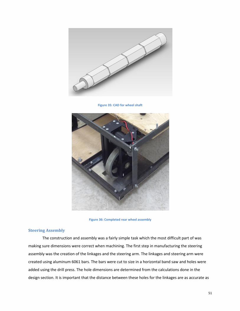
51

Figure 35: CAD for wheel shaft

Figure 36: Completed rear wheel assembly

Steering Assembly

The construction and assembly was a fairly simple task which the most difficult part of was

making sure dimensions were correct when machining. The first step in manufacturing the steering

assembly was the creation of the linkages and the steering arm. The linkages and steering arm were

created using aluminum 6061 bars. The bars were cut to size in a horizontal band saw and holes were

added using the drill press. The hole dimensions are determined from the calculations done in the

design section. It is important that the distance between these holes for the linkages are as accurate as

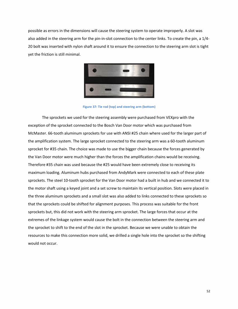
52

possible as errors in the dimensions will cause the steering system to operate improperly. A slot was

also added in the steering arm for the pin-in-slot connection to the center links. To create the pin, a 1/4-

20 bolt was inserted with nylon shaft around it to ensure the connection to the steering arm slot is tight

yet the friction is still minimal.

Figure 37: Tie rod (top) and steering arm (bottom)

The sprockets we used for the steering assembly were purchased from VEXpro with the

exception of the sprocket connected to the Bosch Van Door motor which was purchased from

McMaster. 66-tooth aluminum sprockets for use with ANSI #25 chain where used for the larger part of

the amplification system. The large sprocket connected to the steering arm was a 60-tooth aluminum

sprocket for #35 chain. The choice was made to use the bigger chain because the forces generated by

the Van Door motor were much higher than the forces the amplification chains would be receiving.

Therefore #35 chain was used because the #25 would have been extremely close to receiving its

maximum loading. Aluminum hubs purchased from AndyMark were connected to each of these plate

sprockets. The steel 10-tooth sprocket for the Van Door motor had a built in hub and we connected it to

the motor shaft using a keyed joint and a set screw to maintain its vertical position. Slots were placed in

the three aluminum sprockets and a small slot was also added to links connected to these sprockets so

that the sprockets could be shifted for alignment purposes. This process was suitable for the front

sprockets but, this did not work with the steering arm sprocket. The large forces that occur at the

extremes of the linkage system would cause the bolt in the connection between the steering arm and

the sprocket to shift to the end of the slot in the sprocket. Because we were unable to obtain the

resources to make this connection more solid, we drilled a single hole into the sprocket so the shifting

would not occur.

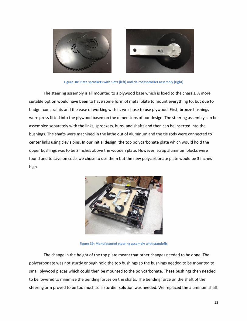
53

Figure 38: Plate sprockets with slots (left) and tie rod/sprocket assembly (right)

The steering assembly is all mounted to a plywood base which is fixed to the chassis. A more

suitable option would have been to have some form of metal plate to mount everything to, but due to

budget constraints and the ease of working with it, we chose to use plywood. First, bronze bushings

were press fitted into the plywood based on the dimensions of our design. The steering assembly can be

assembled separately with the links, sprockets, hubs, and shafts and then can be inserted into the

bushings. The shafts were machined in the lathe out of aluminum and the tie rods were connected to

center links using clevis pins. In our initial design, the top polycarbonate plate which would hold the

upper bushings was to be 2 inches above the wooden plate. However, scrap aluminum blocks were

found and to save on costs we chose to use them but the new polycarbonate plate would be 3 inches

high.

Figure 39: Manufactured steering assembly with standoffs

The change in the height of the top plate meant that other changes needed to be done. The

polycarbonate was not sturdy enough hold the top bushings so the bushings needed to be mounted to

small plywood pieces which could then be mounted to the polycarbonate. These bushings then needed

to be lowered to minimize the bending forces on the shafts. The bending force on the shaft of the

steering arm proved to be too much so a sturdier solution was needed. We replaced the aluminum shaft

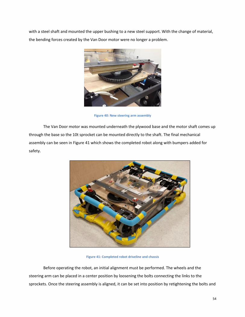
54

with a steel shaft and mounted the upper bushing to a new steel support. With the change of material,

the bending forces created by the Van Door motor were no longer a problem.

Figure 40: New steering arm assembly

The Van Door motor was mounted underneath the plywood base and the motor shaft comes up

through the base so the 10t sprocket can be mounted directly to the shaft. The final mechanical

assembly can be seen in Figure 41 which shows the completed robot along with bumpers added for

safety.

Figure 41: Completed robot driveline and chassis

Before operating the robot, an initial alignment must be performed. The wheels and the

steering arm can be placed in a center position by loosening the bolts connecting the links to the

sprockets. Once the steering assembly is aligned, it can be set into position by retightening the bolts and

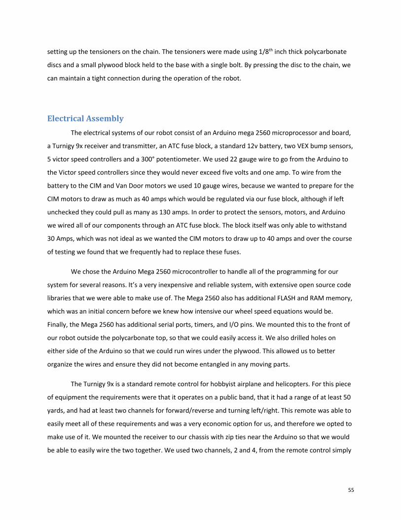
55

setting up the tensioners on the chain. The tensioners were made using 1/8th inch thick polycarbonate

discs and a small plywood block held to the base with a single bolt. By pressing the disc to the chain, we

can maintain a tight connection during the operation of the robot.

Electrical Assembly

The electrical systems of our robot consist of an Arduino mega 2560 microprocessor and board,

a Turnigy 9x receiver and transmitter, an ATC fuse block, a standard 12v battery, two VEX bump sensors,

5 victor speed controllers and a 300° potentiometer. We used 22 gauge wire to go from the Arduino to

the Victor speed controllers since they would never exceed five volts and one amp. To wire from the

battery to the CIM and Van Door motors we used 10 gauge wires, because we wanted to prepare for the

CIM motors to draw as much as 40 amps which would be regulated via our fuse block, although if left

unchecked they could pull as many as 130 amps. In order to protect the sensors, motors, and Arduino

we wired all of our components through an ATC fuse block. The block itself was only able to withstand

30 Amps, which was not ideal as we wanted the CIM motors to draw up to 40 amps and over the course

of testing we found that we frequently had to replace these fuses.

We chose the Arduino Mega 2560 microcontroller to handle all of the programming for our

system for several reasons. It’s a very inexpensive and reliable system, with extensive open source code

libraries that we were able to make use of. The Mega 2560 also has additional FLASH and RAM memory,

which was an initial concern before we knew how intensive our wheel speed equations would be.

Finally, the Mega 2560 has additional serial ports, timers, and I/O pins. We mounted this to the front of

our robot outside the polycarbonate top, so that we could easily access it. We also drilled holes on

either side of the Arduino so that we could run wires under the plywood. This allowed us to better

organize the wires and ensure they did not become entangled in any moving parts.

The Turnigy 9x is a standard remote control for hobbyist airplane and helicopters. For this piece

of equipment the requirements were that it operates on a public band, that it had a range of at least 50

yards, and had at least two channels for forward/reverse and turning left/right. This remote was able to

easily meet all of these requirements and was a very economic option for us, and therefore we opted to

make use of it. We mounted the receiver to our chassis with zip ties near the Arduino so that we would

be able to easily wire the two together. We used two channels, 2 and 4, from the remote control simply

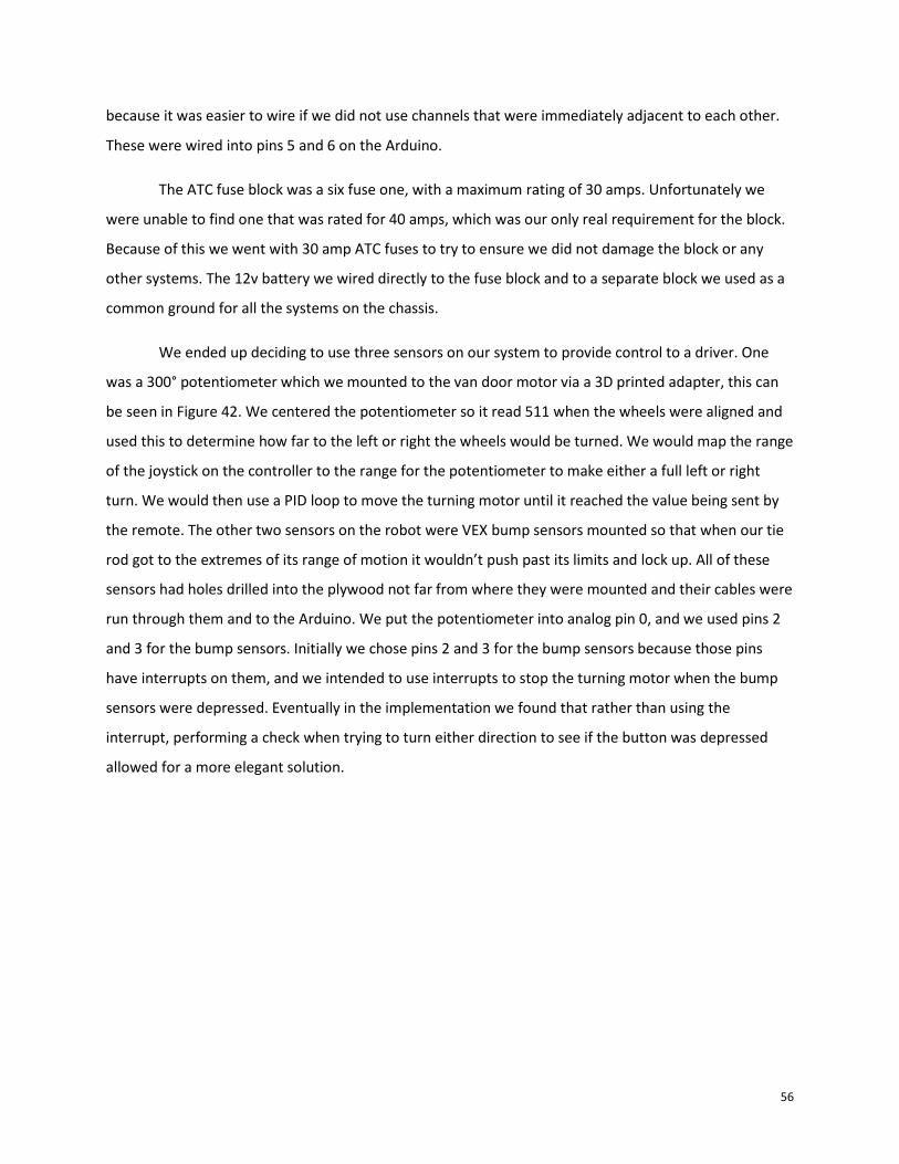
56

because it was easier to wire if we did not use channels that were immediately adjacent to each other.

These were wired into pins 5 and 6 on the Arduino.

The ATC fuse block was a six fuse one, with a maximum rating of 30 amps. Unfortunately we

were unable to find one that was rated for 40 amps, which was our only real requirement for the block.

Because of this we went with 30 amp ATC fuses to try to ensure we did not damage the block or any

other systems. The 12v battery we wired directly to the fuse block and to a separate block we used as a

common ground for all the systems on the chassis.

We ended up deciding to use three sensors on our system to provide control to a driver. One

was a 300° potentiometer which we mounted to the van door motor via a 3D printed adapter, this can

be seen in Figure 42. We centered the potentiometer so it read 511 when the wheels were aligned and

used this to determine how far to the left or right the wheels would be turned. We would map the range

of the joystick on the controller to the range for the potentiometer to make either a full left or right

turn. We would then use a PID loop to move the turning motor until it reached the value being sent by

the remote. The other two sensors on the robot were VEX bump sensors mounted so that when our tie

rod got to the extremes of its range of motion it wouldn’t push past its limits and lock up. All of these

sensors had holes drilled into the plywood not far from where they were mounted and their cables were

run through them and to the Arduino. We put the potentiometer into analog pin 0, and we used pins 2

and 3 for the bump sensors. Initially we chose pins 2 and 3 for the bump sensors because those pins

have interrupts on them, and we intended to use interrupts to stop the turning motor when the bump

sensors were depressed. Eventually in the implementation we found that rather than using the

interrupt, performing a check when trying to turn either direction to see if the button was depressed

allowed for a more elegant solution.

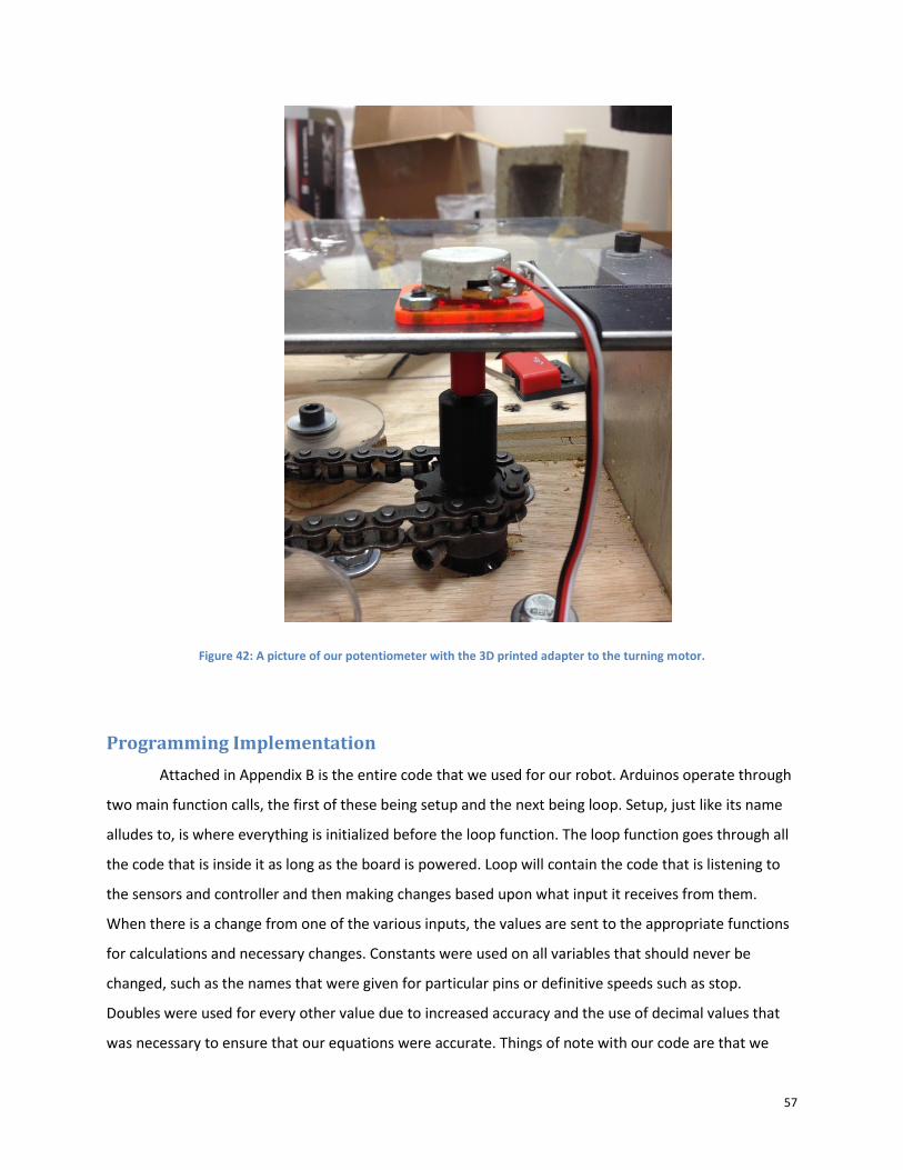
57

Figure 42: A picture of our potentiometer with the 3D printed adapter to the turning motor.

Programming Implementation

Attached in Appendix B is the entire code that we used for our robot. Arduinos operate through

two main function calls, the first of these being setup and the next being loop. Setup, just like its name

alludes to, is where everything is initialized before the loop function. The loop function goes through all

the code that is inside it as long as the board is powered. Loop will contain the code that is listening to

the sensors and controller and then making changes based upon what input it receives from them.

When there is a change from one of the various inputs, the values are sent to the appropriate functions

for calculations and necessary changes. Constants were used on all variables that should never be

changed, such as the names that were given for particular pins or definitive speeds such as stop.

Doubles were used for every other value due to increased accuracy and the use of decimal values that

was necessary to ensure that our equations were accurate. Things of note with our code are that we

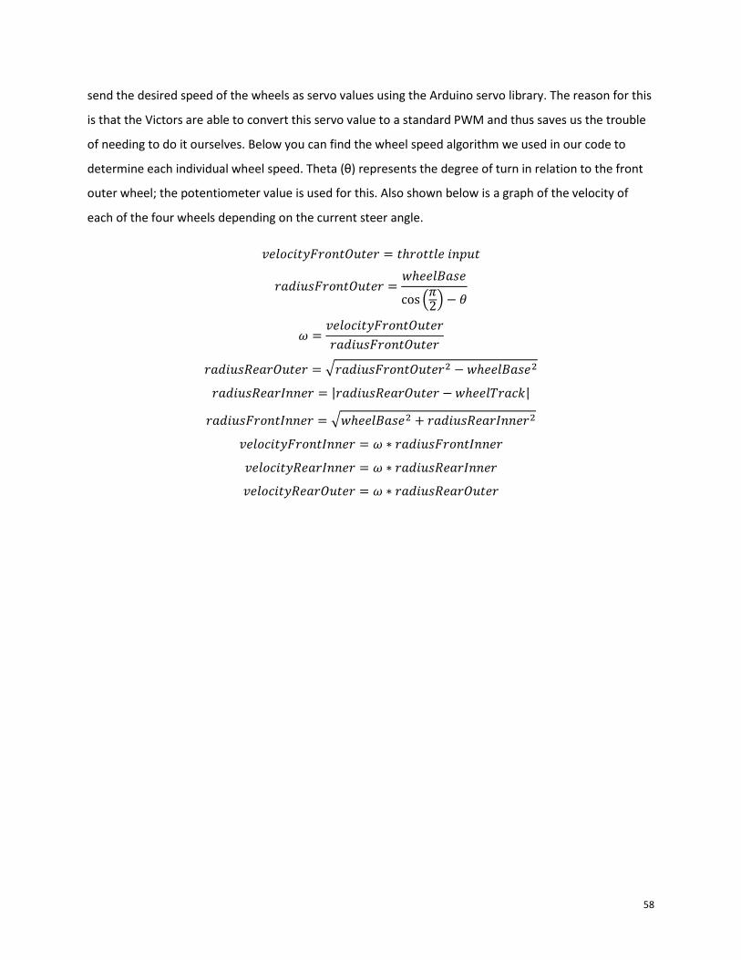
58

send the desired speed of the wheels as servo values using the Arduino servo library. The reason for this

is that the Victors are able to convert this servo value to a standard PWM and thus saves us the trouble

of needing to do it ourselves. Below you can find the wheel speed algorithm we used in our code to

determine each individual wheel speed. Theta (θ) represents the degree of turn in relation to the front

outer wheel; the potentiometer value is used for this. Also shown below is a graph of the velocity of

each of the four wheels depending on the current steer angle.

𝑣𝑒𝑙𝑜𝑐𝑖𝑡𝑦𝐹𝑟𝑜𝑛𝑡𝑂𝑢𝑡𝑒𝑟 = 𝑡ℎ𝑟𝑜𝑡𝑡𝑙𝑒 𝑖𝑛𝑝𝑢𝑡

𝑟𝑎𝑑𝑖𝑢𝑠𝐹𝑟𝑜𝑛𝑡𝑂𝑢𝑡𝑒𝑟 =𝑤ℎ𝑒𝑒𝑙𝐵𝑎𝑠𝑒

cos (𝜋2) − 𝜃

𝜔 =𝑣𝑒𝑙𝑜𝑐𝑖𝑡𝑦𝐹𝑟𝑜𝑛𝑡𝑂𝑢𝑡𝑒𝑟

𝑟𝑎𝑑𝑖𝑢𝑠𝐹𝑟𝑜𝑛𝑡𝑂𝑢𝑡𝑒𝑟

𝑟𝑎𝑑𝑖𝑢𝑠𝑅𝑒𝑎𝑟𝑂𝑢𝑡𝑒𝑟 = √𝑟𝑎𝑑𝑖𝑢𝑠𝐹𝑟𝑜𝑛𝑡𝑂𝑢𝑡𝑒𝑟2 − 𝑤ℎ𝑒𝑒𝑙𝐵𝑎𝑠𝑒2

𝑟𝑎𝑑𝑖𝑢𝑠𝑅𝑒𝑎𝑟𝐼𝑛𝑛𝑒𝑟 = |𝑟𝑎𝑑𝑖𝑢𝑠𝑅𝑒𝑎𝑟𝑂𝑢𝑡𝑒𝑟 − 𝑤ℎ𝑒𝑒𝑙𝑇𝑟𝑎𝑐𝑘|

𝑟𝑎𝑑𝑖𝑢𝑠𝐹𝑟𝑜𝑛𝑡𝐼𝑛𝑛𝑒𝑟 = √𝑤ℎ𝑒𝑒𝑙𝐵𝑎𝑠𝑒2 + 𝑟𝑎𝑑𝑖𝑢𝑠𝑅𝑒𝑎𝑟𝐼𝑛𝑛𝑒𝑟2

𝑣𝑒𝑙𝑜𝑐𝑖𝑡𝑦𝐹𝑟𝑜𝑛𝑡𝐼𝑛𝑛𝑒𝑟 = 𝜔 ∗ 𝑟𝑎𝑑𝑖𝑢𝑠𝐹𝑟𝑜𝑛𝑡𝐼𝑛𝑛𝑒𝑟

𝑣𝑒𝑙𝑜𝑐𝑖𝑡𝑦𝑅𝑒𝑎𝑟𝐼𝑛𝑛𝑒𝑟 = 𝜔 ∗ 𝑟𝑎𝑑𝑖𝑢𝑠𝑅𝑒𝑎𝑟𝐼𝑛𝑛𝑒𝑟

𝑣𝑒𝑙𝑜𝑐𝑖𝑡𝑦𝑅𝑒𝑎𝑟𝑂𝑢𝑡𝑒𝑟 = 𝜔 ∗ 𝑟𝑎𝑑𝑖𝑢𝑠𝑅𝑒𝑎𝑟𝑂𝑢𝑡𝑒𝑟

59

Figure 43: Wheel velocity vs. steer angle

This code takes the throttle input from the controller and potentiometer value. From these

inputs and the wheel track and wheel base measurements, we can calculate the speed that each wheel

needs to spin to make a given turn. Wheel track is essentially the width, measured from the center of

one wheel to the center of the other wheel directly across from it. Wheel base is the length which is

measured from the center of one wheel to the center of the wheel directly in line with it.

0

1

2

3

4

5

6

7

8

9

10

0 10 20 30 40 50 60

Wh

eel V

elo

city (

ft/s

)

Front Outer Steer Angle (degrees)

Front Outer Velocity

Front Inner Velocity

Rear Outer Velocity

Rear Inner Velocity

60

Testing and Evaluation

Individual Performance Evaluation

To test our driveline, we were first able to determine its zero radius turning capability, the

ability of the driveline to maintain the 10-foot radius circle, and overall handling and performance.

These evaluations can be done without the need of another robot for comparison. For the circle test, we

drove the robot on a carpeted surface like that which is typically used for FRC competitions. Due to

space limitations and lack of carpet, we were unable to test the 10-foot radius circle capabilities.

However, we were able to test using a 5-foot radius instead. The tighter radius is actually more difficult

to achieve, so the robot should still be capable of the same performance assuming that there was

enough space and the same surface was used. The results of this test are detailed below.

Comparative Performance Evaluation

For the comparative performance evaluation, we created a test course and assembled a team of

drivers to race both our robot and the robot from FRC Team 190’s 2013 competition. Team 190’s 2013

robot is a 6 wheel tank drive driveline with omni wheels in the rear. It uses four CIM motors for driving

the wheels and is nearly identical size and weight to our own driveline making it a great candidate for

comparison considering it uses one of the most common drivelines for FRC robots. We added additional

weights on the bottom platform of our robot so that the two robots had the same weight.

As for the course, it was created by adding modified elements of the standard Emergency

Vehicle Operations Course (EVOC). These course elements ensure that we can examine different aspects

of vehicle performance. Figure 44 shows the course we designed.

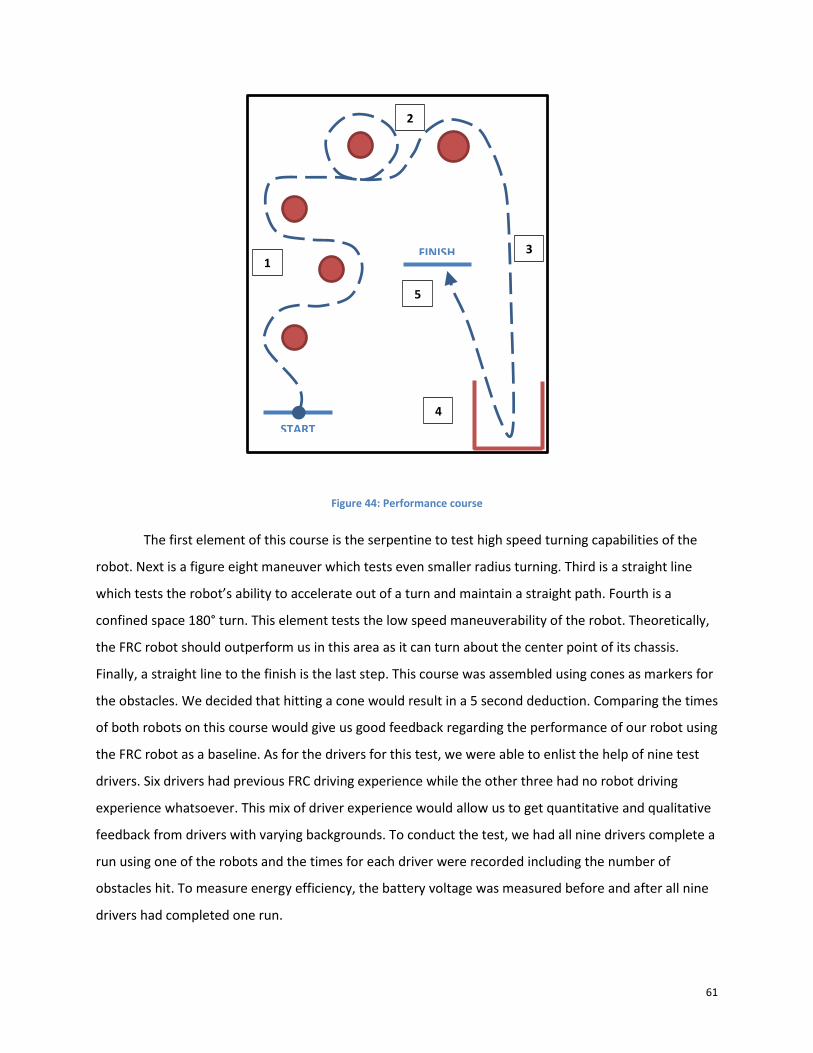
61

Figure 44: Performance course

The first element of this course is the serpentine to test high speed turning capabilities of the

robot. Next is a figure eight maneuver which tests even smaller radius turning. Third is a straight line

which tests the robot’s ability to accelerate out of a turn and maintain a straight path. Fourth is a

confined space 180° turn. This element tests the low speed maneuverability of the robot. Theoretically,

the FRC robot should outperform us in this area as it can turn about the center point of its chassis.

Finally, a straight line to the finish is the last step. This course was assembled using cones as markers for

the obstacles. We decided that hitting a cone would result in a 5 second deduction. Comparing the times

of both robots on this course would give us good feedback regarding the performance of our robot using

the FRC robot as a baseline. As for the drivers for this test, we were able to enlist the help of nine test

drivers. Six drivers had previous FRC driving experience while the other three had no robot driving

experience whatsoever. This mix of driver experience would allow us to get quantitative and qualitative

feedback from drivers with varying backgrounds. To conduct the test, we had all nine drivers complete a

run using one of the robots and the times for each driver were recorded including the number of

obstacles hit. To measure energy efficiency, the battery voltage was measured before and after all nine

drivers had completed one run.

START

FINISH 1

.

2

.

3

.

4

.

5

.

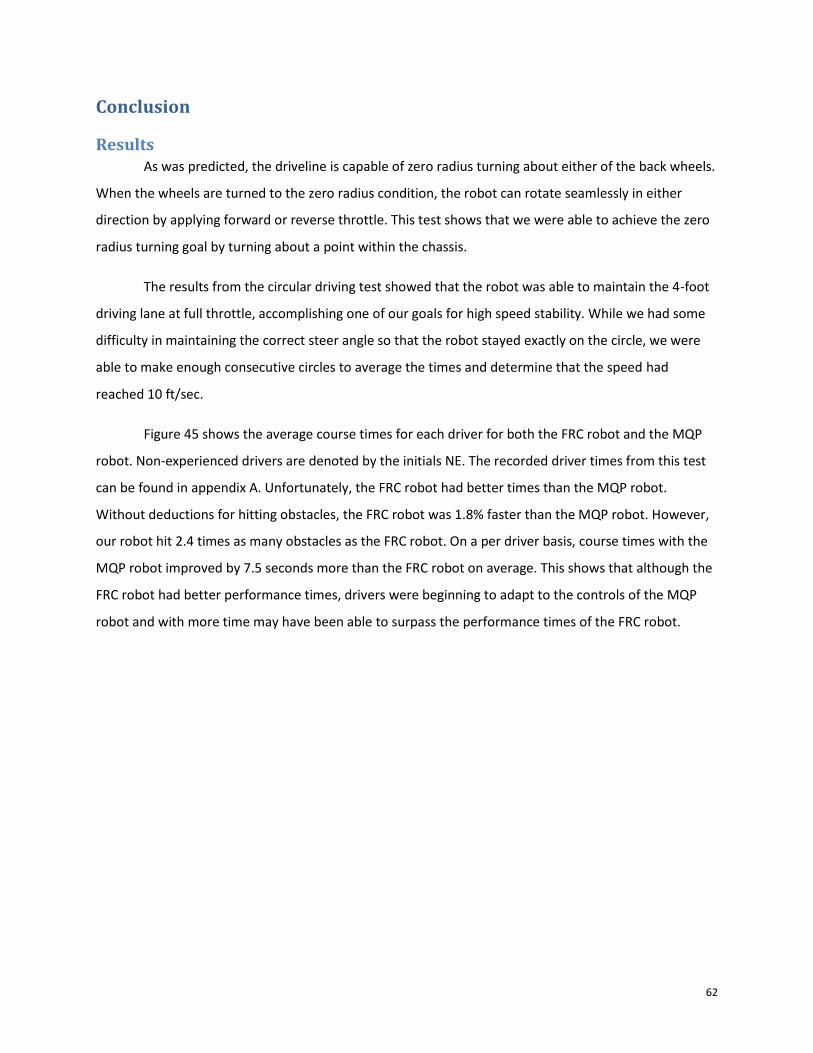
62

Conclusion

Results As was predicted, the driveline is capable of zero radius turning about either of the back wheels.

When the wheels are turned to the zero radius condition, the robot can rotate seamlessly in either

direction by applying forward or reverse throttle. This test shows that we were able to achieve the zero

radius turning goal by turning about a point within the chassis.

The results from the circular driving test showed that the robot was able to maintain the 4-foot

driving lane at full throttle, accomplishing one of our goals for high speed stability. While we had some

difficulty in maintaining the correct steer angle so that the robot stayed exactly on the circle, we were

able to make enough consecutive circles to average the times and determine that the speed had

reached 10 ft/sec.

Figure 45 shows the average course times for each driver for both the FRC robot and the MQP

robot. Non-experienced drivers are denoted by the initials NE. The recorded driver times from this test

can be found in appendix A. Unfortunately, the FRC robot had better times than the MQP robot.

Without deductions for hitting obstacles, the FRC robot was 1.8% faster than the MQP robot. However,

our robot hit 2.4 times as many obstacles as the FRC robot. On a per driver basis, course times with the

MQP robot improved by 7.5 seconds more than the FRC robot on average. This shows that although the

FRC robot had better performance times, drivers were beginning to adapt to the controls of the MQP

robot and with more time may have been able to surpass the performance times of the FRC robot.

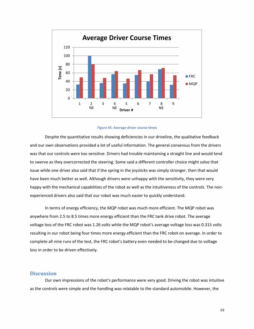
63

Figure 45: Average driver course times

Despite the quantitative results showing deficiencies in our driveline, the qualitative feedback

and our own observations provided a lot of useful information. The general consensus from the drivers

was that our controls were too sensitive. Drivers had trouble maintaining a straight line and would tend

to swerve as they overcorrected the steering. Some said a different controller choice might solve that

issue while one driver also said that if the spring in the joysticks was simply stronger, then that would

have been much better as well. Although drivers were unhappy with the sensitivity, they were very

happy with the mechanical capabilities of the robot as well as the intuitiveness of the controls. The non-

experienced drivers also said that our robot was much easier to quickly understand.

In terms of energy efficiency, the MQP robot was much more efficient. The MQP robot was

anywhere from 2.5 to 8.5 times more energy efficient than the FRC tank drive robot. The average

voltage loss of the FRC robot was 1.26 volts while the MQP robot’s average voltage loss was 0.315 volts

resulting in our robot being four times more energy efficient than the FRC robot on average. In order to

complete all nine runs of the test, the FRC robot’s battery even needed to be changed due to voltage

loss in order to be driven effectively.

Discussion Our own impressions of the robot’s performance were very good. Driving the robot was intuitive

as the controls were simple and the handling was relatable to the standard automobile. However, the

0

20

40

60

80

100

120

1 2 3 4 5 6 7 8 9

Tim

e (

s)

Driver #

Average Driver Course Times

FRC

MQP

NE NE NE

64

controller’s joysticks were very sensitive and it made mid steer angles hard to maintain. Adjustments

were made to the programming to try and make those ranges less sensitive. While these changes

helped, the controller itself just seemed too sensitive to begin with. With our own performance tests,

we found that the robot handled very well despite these sensitivity issues and was even capable of going

from full throttle forward motion to a full throttle zero radius turn with minimal skidding due to its

forward momentum. All of these tests were very promising for future use of this driveline design.

From our observations, we noted that nearly all drivers had a hard time understanding the zero

radius turning capabilities that our robot provided. Especially in the confined space turn, drivers would

have the wheels in the correct full turn and simply accelerate in the wrong direction or turn the wrong

way. Our reasoning was that because the operation of our robot was so similar to that of a common

automobile, the drivers had a harder time adapting to the increased range of motion. Based on all of the

feedback we received, we are very confident that the MQP robot times would beat the FRC times if the

sensitivity of the controls was improved upon and drivers were given more time to learn the capabilities

of our driveline.

In particular, the ability of our root to execute smooth turns and drive in a uniform circle is very

beneficial. This capability is something that most FRC robots cannot achieve, especially tank drive. We

could see that during the serpentine section of the course, drivers quickly learned how to make gradual

turns which cut down on time. The skid steered FRC robot tended to stop after each cone and adjust

their angle before continuing.

Another major advantage that our system has is the increased energy efficiency. While this

advantage to our robot was expected, the degree to which it occurred was surprising. The inherent skid

steering of the tank drive robot was the source of the high inefficiency. The FRC robot’s battery even

had to be changed in order to effectively complete a run with all nine drivers.

The significant improvements that could stand to be made to our design are in the overall size of

our mechanism, the method of driving the tie rod that controls wheel turning, and finally the user

interface. Each of these were designed and built adequately to meet our goals, but could still be better

designed to make for easier use on other systems.

The pin-in-slot system that we used to drive our linkage required both a large amount of torque

to drive at its extreme ranges as well as using up a large portion of the top of the chassis. In order to

make the chassis better able to support additional manipulators and equipment, the system should

65

ideally be made more compact. We suspect that if the equations we developed to find the proper turn

angles were applied to a smaller linkage system, this space could be reduced. Similarly, our pin-in-slot

method of driving the tie rod needed a very large amount of torque to be able to properly position the

wheels when they got close to their extreme ranges. We believe that there is likely a solution for this

that one could create with linkages that would generate the same motion, but require much less torque

at its extremes as well as helping to prevent the problem of the linkages locking up at their extremes. By

changing the pin-in-slot, additional space behind the linkage could be created.

Depending on the application of the robot, having the turning point between the two rear

wheels might be a better choice. We chose to turn about one of the rear wheels for simplicity ad

because our linkage would lock up shortly after that. However, if the linage were modified and actuated

using a different system, the wheels could turn even farther to allow the root to turn about a point at

the center of the rear axle.

The control system we chose was to use was that of a hobby RC airplane remote. The y axis on

the left joystick was used as throttle, and the x axis of the right joystick was used for turning. This system

was chosen in major part for its simplicity and the inexpensiveness of the controller itself. Unfortunately

the range of motion of the controller was not as large as we would have liked and we quickly saw that

people tended to drive at the extremes of the turning range, rather than making use of the middle

ranges. We believe it to be possible to rectify this problem in several ways. One option would be to use

a different controller altogether, such as a hobby RC car remote with a small wheel on it that would be

used for steering, and a simple trigger for throttle. Another potential option is to simply choose a

remote control that gives more force-feedback as you increase the turn range, that way the user gets

more feedback about how far they’re driving the turning mechanism and they are less likely to use its

extremes when they don’t need to.

Social Implications

After completing our prototype, we believe that it could certainly be used for a wide variety of

applications. Any vehicle that is required to operate at high speed as well as make tight turns could

benefit from a system like the one we developed. This includes certain robots, as well as street cars,

trucks, construction equipment, tractors, lawn mowers, and recreational vehicles.

For applications that currently use Ackermann steering, like cars, the impact of our system

would be most significant. It would allow these vehicles to be more maneuverable in confined spaces

66

and perform precise maneuvers with greater speed and ease. One result of this would be that travel

times would be reduced. This would directly make a difference in many peoples' lives, but could also

allow emergency vehicles and law enforcement to reach locations faster. Another result of the increased

maneuverability compared to Ackermann is that some infrastructure could be made more space

efficient. Many of the systems that are currently optimized for typical cars, such as intersections, parking

lots, and garages, could potentially be made smaller.

Another result of using our system over drivelines that are currently used for low speed

maneuverability is the increased efficiency. Energy could be saved in applications that currently involve

tank drive or mecanum drive. While these systems are relatively uncommon, they are so inefficient that

replacing them could have a great impact by reducing fuel costs for those who do use them. Over the

long term, this could also slightly reduce harmful emissions and cut down on the usage of nonrenewable

fuel sources.

The ability to perform a turn in place may open up new possibilities for slow moving

construction and farm equipment as well. If large, heavy machines were able to maneuver themselves

into tight spaces more easily and reach positions that are not currently feasible, it may be possible to

reduce construction timelines and generally increase productivity wherever these vehicles are used. In

some situations, this may even reduce the cost of certain goods and services for consumers.

Final Conclusions

Our design was mechanically a very viable option for future use in either FIRST robotics or

potentially for larger vehicles that need more maneuverability than standard Ackermann can provide. It

was able to meet all of the specifications we set out for it, with the sole exception of being faster than

the FRC Team 190 robot. We believe based on the driver feedback and results of our tests, however,

that this loss was not due to a mechanical failure of our system, but rather that it was due to an

underdeveloped user interface system. The goals that it was able to accomplish are: reach a speed of at

least 10ft/s, maintain a 4 foot lane while driving a 10 foot radius circle, and be able to turn about a point

within the perimeter of the chassis. Some more general goals that we tried to optimize for were to

maximize traction at low speeds by powering each wheel independently, to maximize the energy

efficiency of the system by reducing skidding, limit the degrees of freedom of the system, and finally to

comply with all the FRC rules of the 2013 season. Since we met each of these desired goals with the one

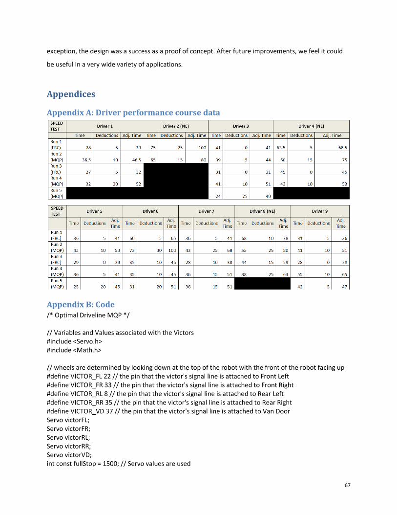
67

exception, the design was a success as a proof of concept. After future improvements, we feel it could

be useful in a very wide variety of applications.

Appendices

Appendix A: Driver performance course data

Appendix B: Code /* Optimal Driveline MQP */ // Variables and Values associated with the Victors #include <Servo.h> #include <Math.h> // wheels are determined by looking down at the top of the robot with the front of the robot facing up #define VICTOR_FL 22 // the pin that the victor's signal line is attached to Front Left #define VICTOR_FR 33 // the pin that the victor's signal line is attached to Front Right #define VICTOR_RL 8 // the pin that the victor's signal line is attached to Rear Left #define VICTOR_RR 35 // the pin that the victor's signal line is attached to Rear Right #define VICTOR_VD 37 // the pin that the victor's signal line is attached to Van Door Servo victorFL; Servo victorFR; Servo victorRL; Servo victorRR; Servo victorVD; int const fullStop = 1500; // Servo values are used

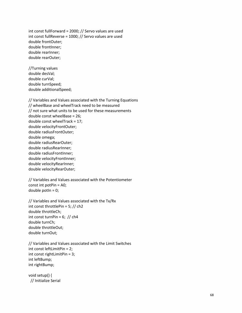
68

int const fullForward = 2000; // Servo values are used int const fullReverse = 1000; // Servo values are used double frontOuter; double frontInner; double rearInner; double rearOuter; //Turning values double desVal; double curVal; double turnSpeed; double additionalSpeed; // Variables and Values associated with the Turning Equations // wheelBase and wheelTrack need to be measured // not sure what units to be used for these measurements double const wheelBase = 26; double const wheelTrack = 17; double velocityFrontOuter; double radiusFrontOuter; double omega; double radiusRearOuter; double radiusRearInner; double radiusFrontInner; double velocityFrontInner; double velocityRearInner; double velocityRearOuter; // Variables and Values associated with the Potentiometer const int potPin = A0; double potIn = 0; // Variables and Values associated with the Tx/Rx int const throttlePin = 5; // ch2 double throttleCh; int const turnPin = 6; // ch4 double turnCh; double throttleOut; double turnOut; // Variables and Values associated with the Limit Switches int const leftLimitPin = 2; int const rightLimitPin = 3; int leftBump; int rightBump; void setup() { // Initialize Serial

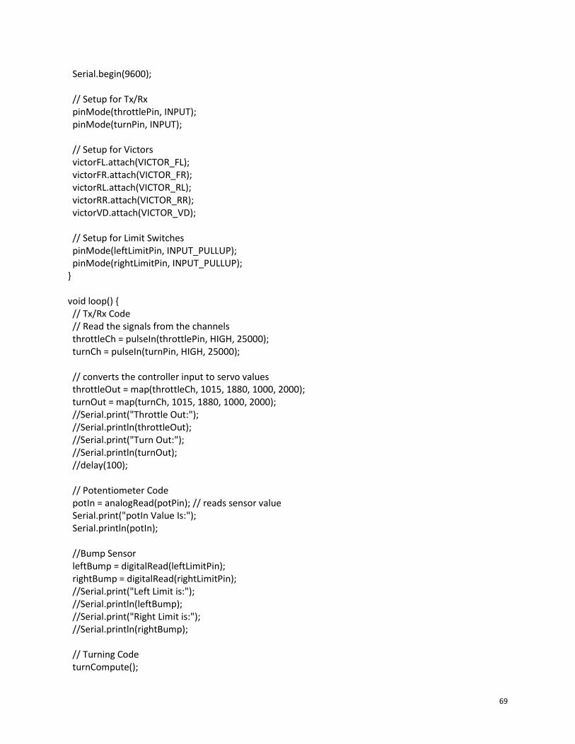
69

Serial.begin(9600); // Setup for Tx/Rx pinMode(throttlePin, INPUT); pinMode(turnPin, INPUT); // Setup for Victors victorFL.attach(VICTOR_FL); victorFR.attach(VICTOR_FR); victorRL.attach(VICTOR_RL); victorRR.attach(VICTOR_RR); victorVD.attach(VICTOR_VD); // Setup for Limit Switches pinMode(leftLimitPin, INPUT_PULLUP); pinMode(rightLimitPin, INPUT_PULLUP); } void loop() { // Tx/Rx Code // Read the signals from the channels throttleCh = pulseIn(throttlePin, HIGH, 25000); turnCh = pulseIn(turnPin, HIGH, 25000); // converts the controller input to servo values throttleOut = map(throttleCh, 1015, 1880, 1000, 2000); turnOut = map(turnCh, 1015, 1880, 1000, 2000); //Serial.print("Throttle Out:"); //Serial.println(throttleOut); //Serial.print("Turn Out:"); //Serial.println(turnOut); //delay(100); // Potentiometer Code potIn = analogRead(potPin); // reads sensor value Serial.print("potIn Value Is:"); Serial.println(potIn); //Bump Sensor leftBump = digitalRead(leftLimitPin); rightBump = digitalRead(rightLimitPin); //Serial.print("Left Limit is:"); //Serial.println(leftBump); //Serial.print("Right Limit is:"); //Serial.println(rightBump); // Turning Code turnCompute();

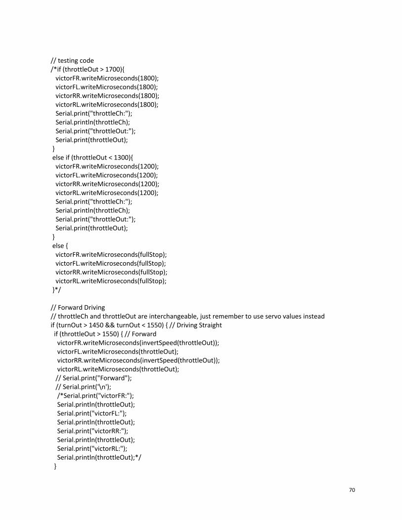
70

// testing code /*if (throttleOut > 1700){ victorFR.writeMicroseconds(1800); victorFL.writeMicroseconds(1800); victorRR.writeMicroseconds(1800); victorRL.writeMicroseconds(1800); Serial.print("throttleCh:"); Serial.println(throttleCh); Serial.print("throttleOut:"); Serial.print(throttleOut); } else if (throttleOut < 1300){ victorFR.writeMicroseconds(1200); victorFL.writeMicroseconds(1200); victorRR.writeMicroseconds(1200); victorRL.writeMicroseconds(1200); Serial.print("throttleCh:"); Serial.println(throttleCh); Serial.print("throttleOut:"); Serial.print(throttleOut); } else { victorFR.writeMicroseconds(fullStop); victorFL.writeMicroseconds(fullStop); victorRR.writeMicroseconds(fullStop); victorRL.writeMicroseconds(fullStop); }*/ // Forward Driving // throttleCh and throttleOut are interchangeable, just remember to use servo values instead if (turnOut > 1450 && turnOut < 1550) { // Driving Straight if (throttleOut > 1550) { // Forward victorFR.writeMicroseconds(invertSpeed(throttleOut)); victorFL.writeMicroseconds(throttleOut); victorRR.writeMicroseconds(invertSpeed(throttleOut)); victorRL.writeMicroseconds(throttleOut); // Serial.print("Forward"); // Serial.print('\n'); /*Serial.print("victorFR:"); Serial.println(throttleOut); Serial.print("victorFL:"); Serial.println(throttleOut); Serial.print("victorRR:"); Serial.println(throttleOut); Serial.print("victorRL:"); Serial.println(throttleOut);*/ }

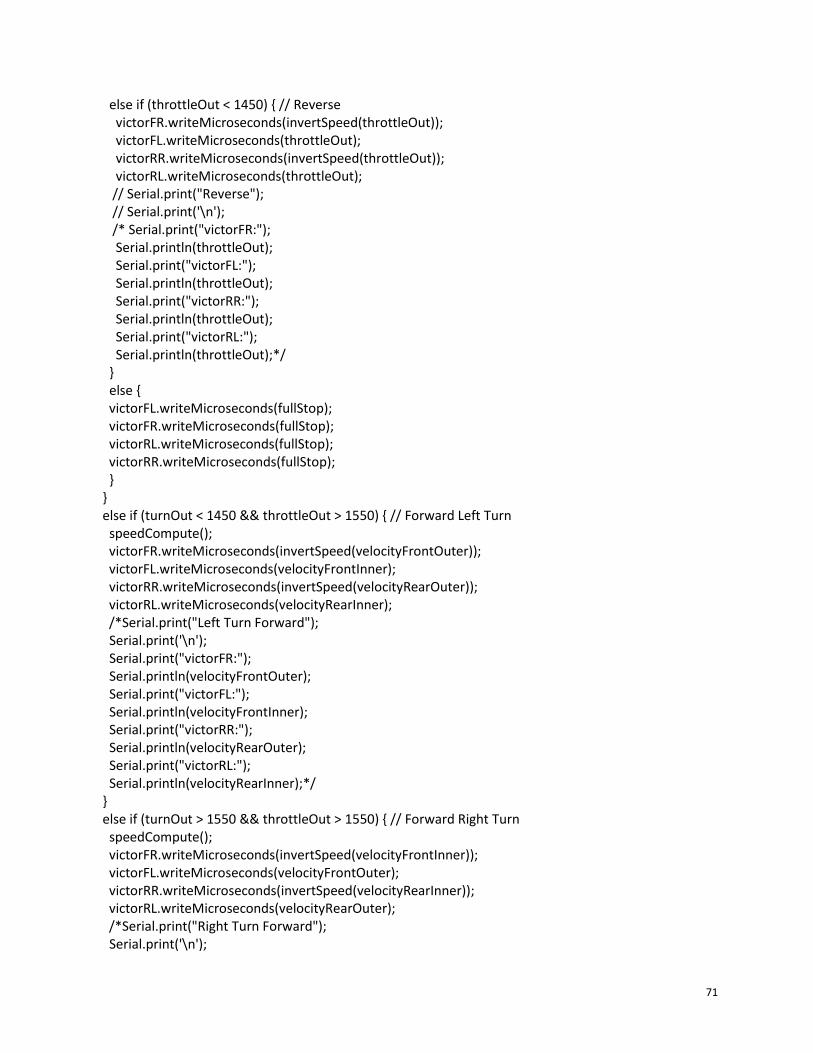
71

else if (throttleOut < 1450) { // Reverse victorFR.writeMicroseconds(invertSpeed(throttleOut)); victorFL.writeMicroseconds(throttleOut); victorRR.writeMicroseconds(invertSpeed(throttleOut)); victorRL.writeMicroseconds(throttleOut); // Serial.print("Reverse"); // Serial.print('\n'); /* Serial.print("victorFR:"); Serial.println(throttleOut); Serial.print("victorFL:"); Serial.println(throttleOut); Serial.print("victorRR:"); Serial.println(throttleOut); Serial.print("victorRL:"); Serial.println(throttleOut);*/ } else { victorFL.writeMicroseconds(fullStop); victorFR.writeMicroseconds(fullStop); victorRL.writeMicroseconds(fullStop); victorRR.writeMicroseconds(fullStop); } } else if (turnOut < 1450 && throttleOut > 1550) { // Forward Left Turn speedCompute(); victorFR.writeMicroseconds(invertSpeed(velocityFrontOuter)); victorFL.writeMicroseconds(velocityFrontInner); victorRR.writeMicroseconds(invertSpeed(velocityRearOuter)); victorRL.writeMicroseconds(velocityRearInner); /*Serial.print("Left Turn Forward"); Serial.print('\n'); Serial.print("victorFR:"); Serial.println(velocityFrontOuter); Serial.print("victorFL:"); Serial.println(velocityFrontInner); Serial.print("victorRR:"); Serial.println(velocityRearOuter); Serial.print("victorRL:"); Serial.println(velocityRearInner);*/ } else if (turnOut > 1550 && throttleOut > 1550) { // Forward Right Turn speedCompute(); victorFR.writeMicroseconds(invertSpeed(velocityFrontInner)); victorFL.writeMicroseconds(velocityFrontOuter); victorRR.writeMicroseconds(invertSpeed(velocityRearInner)); victorRL.writeMicroseconds(velocityRearOuter); /*Serial.print("Right Turn Forward"); Serial.print('\n');

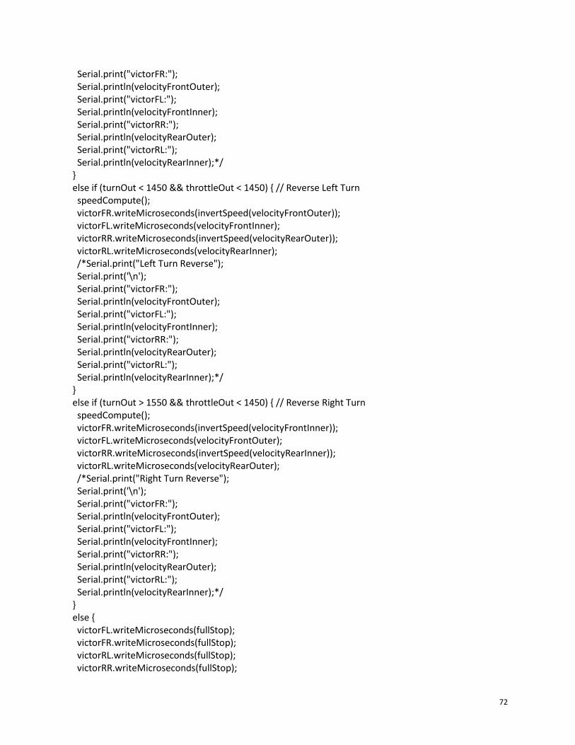
72

Serial.print("victorFR:"); Serial.println(velocityFrontOuter); Serial.print("victorFL:"); Serial.println(velocityFrontInner); Serial.print("victorRR:"); Serial.println(velocityRearOuter); Serial.print("victorRL:"); Serial.println(velocityRearInner);*/ } else if (turnOut < 1450 && throttleOut < 1450) { // Reverse Left Turn speedCompute(); victorFR.writeMicroseconds(invertSpeed(velocityFrontOuter)); victorFL.writeMicroseconds(velocityFrontInner); victorRR.writeMicroseconds(invertSpeed(velocityRearOuter)); victorRL.writeMicroseconds(velocityRearInner); /*Serial.print("Left Turn Reverse"); Serial.print('\n'); Serial.print("victorFR:"); Serial.println(velocityFrontOuter); Serial.print("victorFL:"); Serial.println(velocityFrontInner); Serial.print("victorRR:"); Serial.println(velocityRearOuter); Serial.print("victorRL:"); Serial.println(velocityRearInner);*/ } else if (turnOut > 1550 && throttleOut < 1450) { // Reverse Right Turn speedCompute(); victorFR.writeMicroseconds(invertSpeed(velocityFrontInner)); victorFL.writeMicroseconds(velocityFrontOuter); victorRR.writeMicroseconds(invertSpeed(velocityRearInner)); victorRL.writeMicroseconds(velocityRearOuter); /*Serial.print("Right Turn Reverse"); Serial.print('\n'); Serial.print("victorFR:"); Serial.println(velocityFrontOuter); Serial.print("victorFL:"); Serial.println(velocityFrontInner); Serial.print("victorRR:"); Serial.println(velocityRearOuter); Serial.print("victorRL:"); Serial.println(velocityRearInner);*/ } else { victorFL.writeMicroseconds(fullStop); victorFR.writeMicroseconds(fullStop); victorRL.writeMicroseconds(fullStop); victorRR.writeMicroseconds(fullStop);

73

/*victorVD.writeMicroseconds(fullStop); Serial.println("Stop");*/ } } // End of void loop() // Start of helper functions int invertSpeed (int x) { // used to make sure all wheels are going right direction int y = 0; if (x > 1500) { y = 2000 - x; return 1000 + y; } if (x < 1500) { y = x - 1000; return 2000 - y; } } double potRadVal (double x) { // converts pot value to Radians to use with cos // 472.5 is dead center of 0-945 output // about 1 ticks for every degree of rotation // front wheels have a total movement of 147° // 0 to 90° if front inner // 0 to 57° if front outer // 0° is straight double y = 0; if (x > 513) { y = (x/8.275)-57; return y*(3.14/180); // converts from degrees to radians } else if (x < 431) { y = (-x/8.275)+57; return y*(3.14/180); // converts from degrees to radians } else { return 0; } } double stickToPot (double x) { // converts the turn stick input to Pot Values double y = 0; if (x <= 1450) { // left side of turn stick to pot values if (x >= 1060) { // between 30 degree and 0 y = x*0.8-742; return y; } else { // greater than 30 degree y = x*1.7391-1737.5;

74

return y; } } else if (x >= 1550) { // right side of turn stick of pot values if (x <= 1940) { // between 30 degree and 0 y = x*0.8-742; return y; } else { // greater than 30 degree y = x*1.7391-2563.9; return y; } } else { return 435; // theoretical center for pot } } double voltageToServo (double x) { // convert from voltage to servo return x*38.5+1500; } double servoToVoltage (double x) { // convert from servo to voltage return (x/38.5)-38.5; } void speedCompute () { velocityFrontOuter = servoToVoltage(throttleOut); radiusFrontOuter = wheelBase/(cos((3.14/2)-potRadVal(potIn))); omega = velocityFrontOuter/radiusFrontOuter; radiusRearOuter = sqrt(pow(radiusFrontOuter,2)-pow(wheelBase,2)); radiusRearInner = abs(radiusRearOuter-wheelTrack); radiusFrontInner = sqrt(pow(wheelBase,2)+pow(radiusRearInner,2)); velocityFrontInner = omega*radiusFrontInner; velocityRearInner = omega*radiusRearInner; velocityRearOuter = omega*radiusRearOuter; velocityFrontOuter = voltageToServo(velocityFrontOuter); velocityFrontInner = voltageToServo(velocityFrontInner); velocityRearOuter = voltageToServo(velocityRearOuter); velocityRearInner = voltageToServo(velocityRearInner); } void turnCompute () { // Code to drive van door motor to desired position curVal = potIn/945; // set value of current pot position using range of 1000 to get % of turn desVal = stickToPot(turnOut)/945; // set value of desired positon using % of turn

75

//Serial.print("potIn is:"); //Serial.println(potIn); //Serial.println("Pot Degree Val"); //Serial.println(potRadVal(potIn)); if ((curVal - .025) <= desVal && (curVal + .025) >= desVal) { victorVD.writeMicroseconds(fullStop); //Serial.println("victorVD is stopped:"); //Serial.println(turnCh); } if (curVal >= desVal && rightBump == 1 ) { //turn left additionalSpeed = (0.5 - desVal) * 800; turnSpeed = ((curVal - desVal) * 1000) + additionalSpeed; if (turnSpeed < 150) { turnSpeed = 150; } if (turnSpeed > 500) { turnSpeed = 500; } victorVD.writeMicroseconds(1500 - turnSpeed); //victorVD.writeMicroseconds(1100); //Serial.println("victorVD is turning left"); //Serial.println(1500-turnSpeed); } if (curVal <= desVal && leftBump == 1) { //turn right additionalSpeed = (desVal - 0.5) * 700; turnSpeed = ((desVal - curVal) * 1000) + additionalSpeed; if (turnSpeed < 50) { turnSpeed = 50; } if (turnSpeed > 500) { turnSpeed = 500; } victorVD.writeMicroseconds(1500 + turnSpeed); //victorVD.writeMicroseconds(1900); //Serial.println("victorVD is turning right"); //Serial.println(1500 + turnSpeed); } } // Liam's Turn Equation /*void turnCompute () { // Code to drive van door motor to desired position curVal = (potIn)/945; //set value of current pot position using range of 1000 to get % of turn desVal = (turnOut-1000)/1000; //set value of desired positon using % of turn //Serial.print("potIn is:"); //Serial.println(potIn); //Serial.println("Pot Degree Val");

76

//Serial.println(potRadVal(potIn)); if ((curVal - .05) <= desVal && (curVal + .05) >= desVal) { victorVD.writeMicroseconds(fullStop); //Serial.println("victorVD is stopped:"); //Serial.println(turnCh); } if (curVal >= desVal && rightBump == 1 ) { //turn left additionalSpeed = (0.5 - desVal) * 800; turnSpeed = ((curVal - desVal) * 1000) + additionalSpeed; if (turnSpeed < 50) { turnSpeed = 50; } if (turnSpeed > 500) { turnSpeed = 500; } victorVD.writeMicroseconds(1500 - turnSpeed); //victorVD.writeMicroseconds(1100); //Serial.println("victorVD is turning left"); //Serial.println(1500-turnSpeed); } if (curVal <= desVal && leftBump == 1) { //turn right additionalSpeed = (desVal - 0.5) * 800; turnSpeed = ((desVal - curVal) * 1000) + additionalSpeed; if (turnSpeed < 50) { turnSpeed = 50; } if (turnSpeed > 500) { turnSpeed = 500; } victorVD.writeMicroseconds(1500 + turnSpeed); //victorVD.writeMicroseconds(1900); //Serial.println("victorVD is turning right"); //Serial.println(1500 + turnSpeed); } }*/ // End

77

Appendix C: FRC Motor Data

Appendix D: Power Requirement Data

Steer

Angles

Linkage

Angles

Coeffici

ent of

Friction

Max

Weight

(N)

Wheel Shaft

Torque

(Nm)

Linkage

Shaft Torque

(Nm)

Arm Force

Needed (N)

Steer Arm

Torque

(Nm)

Arm

Rotational

Speed (rad/s)

Power

Needed

(W)

-19 10.25 0.65 533.786 4.406403 13.21921 88.14699 11.19467 0.785398 8.792271

-18 11.25 0.65 533.786 4.406403 13.21921 88.43957 11.23182 0.785398 8.821455

-17 12.25 0.65 533.786 4.406403 13.21921 88.76122 11.27267 0.785398 8.853538

-16 13.25 0.65 533.786 4.406403 13.21921 89.11246 11.31728 0.785398 8.888573

-15 14.25 0.65 533.786 4.406403 13.21921 89.49387 11.36572 0.785398 8.926617

-14 15.25 0.65 533.786 4.406403 13.21921 89.90606 11.41807 0.785398 8.967731

-13 16.25 0.65 533.786 4.406403 13.21921 90.34971 11.47441 0.785398 9.011983

-12 17.25 0.65 533.786 4.406403 13.21921 90.82556 11.53485 0.785398 9.059447

-11 18.25 0.65 533.786 4.406403 13.21921 91.33443 11.59947 0.785398 9.110204

-10 19.25 0.65 533.786 4.406403 13.21921 91.87717 11.6684 0.785398 9.16434

-9 20.25 0.65 533.786 4.406403 13.21921 92.45473 11.74175 0.785398 9.221949

-8 21.25 0.65 533.786 4.406403 13.21921 93.06813 11.81965 0.785398 9.283133

-7 22.25 0.65 533.786 4.406403 13.21921 93.71845 11.90224 0.785398 9.348

-6 23.25 0.65 533.786 4.406403 13.21921 94.40689 11.98968 0.785398 9.416669

-5 24.25 0.65 533.786 4.406403 13.21921 95.13472 12.08211 0.785398 9.489266

-4 25.25 0.65 533.786 4.406403 13.21921 95.90329 12.17972 0.785398 9.565928

-3 26.25 0.65 533.786 4.406403 13.21921 96.71408 12.28269 0.785398 9.646801

78

-2 27.25 0.65 533.786 4.406403 13.21921 97.56868 12.39122 0.785398 9.732043

-1 28.25 0.65 533.786 4.406403 13.21921 98.46877 12.50553 0.785398 9.821823

0 29.25 0.65 533.786 4.406403 13.21921 99.41619 12.62586 0.785398 9.916324

1 30.25 0.65 533.786 4.406403 13.21921 100.4129 12.75244 0.785398 10.01574

2 31.25 0.65 533.786 4.406403 13.21921 101.461 12.88555 0.785398 10.12029

3 32.25 0.65 533.786 4.406403 13.21921 102.5628 13.02548 0.785398 10.23019

4 33.25 0.65 533.786 4.406403 13.21921 103.7207 13.17253 0.785398 10.34568

5 34.25 0.65 533.786 4.406403 13.21921 104.9375 13.32706 0.785398 10.46705

6 35.25 0.65 533.786 4.406403 13.21921 106.2158 13.4894 0.785398 10.59455

7 36.25 0.65 533.786 4.406403 13.21921 107.5588 13.65997 0.785398 10.72851

8 37.25 0.65 533.786 4.406403 13.21921 108.9699 13.83917 0.785398 10.86926

9 38.25 0.65 533.786 4.406403 13.21921 110.4525 14.02747 0.785398 11.01715

10 39.25 0.65 533.786 4.406403 13.21921 112.0107 14.22535 0.785398 11.17257

11 40.25 0.65 533.786 4.406403 13.21921 113.6485 14.43336 0.785398 11.33593

12 41.25 0.65 533.786 4.406403 13.21921 115.3706 14.65207 0.785398 11.50771

13 42.25 0.65 533.786 4.406403 13.21921 117.182 14.88211 0.785398 11.68838

14 43.25 0.65 533.786 4.406403 13.21921 119.088 15.12417 0.785398 11.8785

15 44.25 0.65 533.786 4.406403 13.21921 121.0945 15.379 0.785398 12.07864

16 45.25 0.65 533.786 4.406403 13.21921 123.208 15.64741 0.785398 12.28945

17 46.25 0.65 533.786 4.406403 13.21921 125.4354 15.9303 0.785398 12.51163

18 47.25 0.65 533.786 4.406403 13.21921 127.7845 16.22863 0.785398 12.74594

19 48.25 0.65 533.786 4.406403 13.21921 130.2637 16.54349 0.785398 12.99323

20 49.25 0.65 533.786 4.406403 13.21921 132.8823 16.87605 0.785398 13.25442

21 50.25 0.65 533.786 4.406403 13.21921 135.6505 17.22761 0.785398 13.53054

22 51.25 0.65 533.786 4.406403 13.21921 138.5796 17.59961 0.785398 13.8227

23 52.25 0.65 533.786 4.406403 13.21921 141.6821 17.99363 0.785398 14.13216

24 53.25 0.65 533.786 4.406403 13.21921 144.9719 18.41143 0.785398 14.4603

25 54.25 0.65 533.786 4.406403 13.21921 148.4643 18.85497 0.785398 14.80866

26 55.25 0.65 533.786 4.406403 13.21921 152.1767 19.32644 0.785398 15.17895

27 56.25 0.65 533.786 4.406403 13.21921 156.1283 19.82829 0.785398 15.5731

28 57.25 0.65 533.786 4.406403 13.21921 160.3407 20.36327 0.785398 15.99327

29 58.25 0.65 533.786 4.406403 13.21921 164.8383 20.93447 0.785398 16.44189

30 59.25 0.65 533.786 4.406403 13.21921 169.6487 21.54539 0.785398 16.92171

Appendix E: Bosch Van Door Motor Output Data Steer Angles Linkage Angles Steer Arm Force (N) Tie Rod Force (N) Linkage Shaft Torque (Nm) Wheel Shaft Torque (Nm)

-19 10.25 498.38 490.4262 74.74095 24.91365

-18 11.25 498.38 488.8038 74.49369 24.83123

-17 12.25 498.38 487.0324 74.22374 24.74125

-16 13.25 498.38 485.1128 73.93118 24.64373

-15 14.25 498.38 483.0453 73.6161 24.5387

-14 15.25 498.38 480.8307 73.2786 24.4262

-13 16.25 498.38 478.4696 72.91877 24.30626

79

-12 17.25 498.38 475.9628 72.53674 24.17891

-11 18.25 498.38 473.3111 72.1326 24.0442

-10 19.25 498.38 470.5151 71.7065 23.90217

-9 20.25 498.38 467.5758 71.25855 23.75285

-8 21.25 498.38 464.4941 70.7889 23.5963

-7 22.25 498.38 461.2709 70.29768 23.43256

-6 23.25 498.38 457.9072 69.78505 23.26168

-5 24.25 498.38 454.404 69.25116 23.08372

-4 25.25 498.38 450.7624 68.69618 22.89873

-3 26.25 498.38 446.9834 68.12028 22.70676

-2 27.25 498.38 443.0684 67.52362 22.50787

-1 28.25 498.38 439.0183 66.90639 22.30213

0 29.25 498.38 434.8346 66.26879 22.0896

1 30.25 498.38 430.5183 65.61099 21.87033

2 31.25 498.38 426.071 64.93322 21.64441

3 32.25 498.38 421.4938 64.23566 21.41189

4 33.25 498.38 416.7883 63.51854 21.17285

5 34.25 498.38 411.9558 62.78206 20.92735

6 35.25 498.38 406.9978 62.02647 20.67549

7 36.25 498.38 401.9159 61.25198 20.41733

8 37.25 498.38 396.7115 60.45883 20.15294

9 38.25 498.38 391.3863 59.64726 19.88242

10 39.25 498.38 385.9418 58.81753 19.60584

11 40.25 498.38 380.3798 57.96988 19.32329

12 41.25 498.38 374.7019 57.10457 19.03486

13 42.25 498.38 368.9099 56.22187 18.74062

14 43.25 498.38 363.0055 55.32204 18.44068

15 44.25 498.38 356.9906 54.40536 18.13512

16 45.25 498.38 350.8669 53.47211 17.82404

17 46.25 498.38 344.6363 52.52257 17.50752

18 47.25 498.38 338.3007 51.55703 17.18568

19 48.25 498.38 331.8621 50.57578 16.85859

20 49.25 498.38 325.3224 49.57913 16.52638

21 50.25 498.38 318.6836 48.56738 16.18913

22 51.25 498.38 311.9477 47.54084 15.84695

23 52.25 498.38 305.1168 46.49981 15.49994

24 53.25 498.38 298.193 45.44462 15.14821

25 54.25 498.38 291.1783 44.37558 14.79186

26 55.25 498.38 284.075 43.29303 14.43101

27 56.25 498.38 276.8851 42.19729 14.06576

28 57.25 498.38 269.6109 41.08869 13.69623

29 58.25 498.38 262.2545 39.96759 13.32253

30 59.25 498.38 254.8182 38.8343 12.94477