Embed Size (px)
Citation preview
DEPARTMENT OF ECONOMICS AND FINANCE
COLLEGE OF BUSINESS AND ECONOMICS
UNIVERSITY OF CANTERBURY
CHRISTCHURCH, NEW ZEALAND
The Timeless Perspective vs. Discretion: Theory and
Monetary Policy Implications for an Open Economy
Alfred V Guender
WORKING PAPER
No. 19/2011
Department of Economics and Finance College of Business and Economics
University of Canterbury Private Bag 4800, Christchurch
New Zealand
1
The Timeless Perspective vs. Discretion: Theory and Monetary
Policy Implications for an Open Economy
Revised on April 13, 2011
Alfred V Guender
Department of Economics
University of Canterbury
Christchurch, New Zealand
Abstract:
Compared to the standard Phillips curve, an open-economy version that features a real exchange
rate channel leads to a markedly different target rule in a New Keynesian optimizing framework.
Under optimal policy from a timeless perspective (TP) the target rule involves additional history
dependence in the form of lagged inflation. The target rule also depends on more parameters,
notably the discount factor as well as two IS and two Phillips curve parameters. Stabilization policy
in this open economy model is no longer isomorphic to policy in a closed economy. Because of the
additional history dependence in an open economy target rule price level targeting is no longer
consistent with optimal policy. The gains from commitment are smaller in economies where the real
exchange rate channel exerts a direct effect on inflation in the Phillips curve.
Key Words: Timeless Perspective, Discretion, Price Level Targeting, Exchange Rate Channel.
JEL Classification Codes: E52, F41
______________________________________________________________________________ The author wishes to thank two referees, Richard Froyen, Christina Gerberding, and Michael Scharnagl for providing
helpful comments. Thanks also to seminar participants at the University of Cape Town, University of Graz, Macquarie
University, and Monash University. The research support of the Deutsche Bundesbank is gratefully acknowledged. The
usual disclaimer applies. E-mail: [email protected] Fax: (64)-3-364-2635. Postal Address: Private Bag
4800, Christchurch 8041, New Zealand.

2
Introduction
For some time now central banks and academics have been preoccupied with the way
monetary policy ought to be conducted in an era of relative price stability. Woodford (1999a)
proposes that the course of monetary policy in a forward-looking New Keynesian framework be set
from a timeless perspective (commitment). This form of policy has a number of desirable features.
To begin with, policy from a timeless perspective introduces history-dependence into the conduct of
monetary policy because it is based on an optimal policy rule that depends on the change in the
output gap. The policy instrument responds to a cost-push shock in the current and subsequent
periods until the target variables return to their original targets. The gradual adjustment process gives
rise to persistence in the behavior of the output gap and the rate of inflation. Because the conduct of
policy is history-dependent under policy from a timeless perspective, this strategy dominates pure
discretion under which the response of the target variables to the cost-push shock is confined to the
current period. Moreover, since policy from a timeless perspective is a time-consistent form of
optimal policy under commitment it serves as a standard of comparison for forms of discretionary
policy that also inject an element of history-dependence into policymaking such as price-level
targeting, a speed limit policy, nominal income growth targeting, average inflation targeting or
money growth targeting. Jensen (2002), Néssen and Vestin (2005), Soederstroem (2005), Vestin
(2006), and Walsh (2003) evaluate the aforementioned discretionary strategies in a closed economy
setting and verify to what extent these policies achieve the optimal stabilization results under policy
from a timeless perspective.
This paper focuses on two key differences between policy in an open and a closed economy.
First, it analyzes optimal monetary policy from a timeless perspective in a simple forward-looking
framework to show that the open-economy target rule is far more complex than its closed-economy
counterpart. Optimal stabilization policy in this open economy model is no longer isomorphic to
policy in a closed economy. Second, the paper examines the connection between optimal policy and
price level targeting and finds that the latter is not synonymous with the former in the proposed
open economy model. Central to our discussion of policy in an open economy is a Phillips curve
that features a real exchange rate channel. This exchange rate channel appears in the aggregate
Phillips curve because domestic firms are concerned about their competitiveness at home and in
world markets where their products compete with those produced by foreign firms. Briefly, an
important objective of the typical cost-minimizing domestic firm is to avoid fluctuations in its firm-
specific terms of trade. Hence an incipient rise in the foreign price of the competing foreign good or

3
a rise in the nominal exchange rate leads the typical domestic firm to raise the price of its output.
Thus external factors induce a firm to alter the price of output, which it sets in domestic currency.
Earlier contributions that examine the implications of the existence of an exchange rate channel
for the conduct of monetary policy are Ball (1999), Walsh (1999), Svensson (2000), and Guender
(2006). Ball motivates the real exchange rate channel in the Phillips curve in a backward-looking
framework by assuming that foreign producers are concerned only about receipts in their home
currency. Any change in the nominal exchange rate is offset by adjusting the nominal price of the
good in the foreign country. Positing a linear target rule, Ball finds that optimal policy requires a
central bank to follow a monetary conditions index rather than a Taylor-type rule. Walsh (1999)
derives an open-economy Phillips curve in a forward-looking model where the nominal wage
demands are tied to the CPI. In a model that mixes elements of backward- and forward-looking
behavior, Svensson (2000) introduces a Phillips curve where the expectation, formed in the past, of
the change in the real exchange rate affects the current rate of inflation. He discusses a number of
different policy strategies under discretion but does not derive the underlying endogenous target
rules. Such an explicit target rule is derived in a forward-looking open economy model by Guender
(2006) where firms are guided in their domestic pricing decisions by a benchmark price that is set in
the world market. Such pricing behavior at the firm-level gives rise to an aggregate Phillips curve
that depends on the real exchange rate and a target rule guiding optimal monetary policy that
includes demand-side parameters. Guender considers only optimal policy under discretion. 1
Other contributions downplay or dismiss the importance of a real exchange rate channel in the
Phillips curve. Drawing on empirical evidence that shows only weak correlations between changes
in the nominal exchange rates and inflation rates for a number of countries, McCallum and Nelson
(2000, p. 89) are sceptical about the existence of a direct exchange rate channel and its relevance in
policymaking. Moreover, in their theoretical set-up of an open economy the effect of the real
exchange rate on the output gap is neutralized as it affects both the level of actual output and the
level of potential output in the same way. As a consequence, their Phillips curve is the same as in a
closed economy. Clarida, Gali, and Gertler (2001, 2002) and Gali and Monacelli (2005) derive
essentially a closed-economy Phillips curve too except that the coefficient on marginal cost is
sensitive to the degree of openness of the economy. These papers assume that firms that operate in
small open economies set domestic prices without reference to world market prices or consideration
of the effects of terms of trade changes on their competitiveness.
1 The design of optimal monetary policy is sensitive to the degree of exchange rate pass-through. Monacelli (2005)
argues that incomplete exchange rate pass-through drives a wedge between policymaking in open versus closed
economies. He derives an open economy Phillips curve where the deviation of the world price from the domestic
currency price of imports affects domestic and CPI inflation.

4
This paper takes a contrary view. It emphasizes that domestic firms value stability of their
terms of trade in addition to stable prices. This concern forces cost-minimizing domestic firms to
take account of expected changes in their firm-specific terms of trade when altering the domestic
price of output. Changes in the nominal exchange rate and changes in the price charged by
competing foreign firms are beyond the control of the typical domestic firm. Yet such changes
affect its competitiveness. The only way that a domestic firm can counteract such pressure is to
adjust its domestic price in such a way so that the overall cost to the firm is minimized. If such
pricing behavior applies to the typical firm, aggregation over all firms leads to a Phillips curve
where the expected change in the real exchange rate impacts on domestic inflation.2
The implications for optimal monetary policy are stark. Once the existence of a real exchange
rate channel in the Phillips curve is acknowledged, the optimal target rule under policy from a
timeless perspective becomes vastly different from the standard target rule.3 The new target rule
depends on multiple parameters that appear in both the IS relation and the Phillips curve as well as
on the discount factor. The proposed target rule is history-dependent too but differs from the
standard target rule in a critical way: under policy from a timeless perspective the proposed target
rule also features the lagged rate of inflation in addition to the lagged output gap. However, unlike
the output gap, the rate of inflation does not enter the target rule in first-difference form.
Optimal stabilization policy changes dramatically. In the absence of a real exchange rate
channel in the Phillips curve it is optimal for the policymaker to fix the output gap as doing so
ensures an optimal response to demand-side disturbances and leaves domestic inflation unaffected.
If this channel does exist, however, the policymaker can no longer perfectly offset demand-side
disturbances. Specifically, the policymaker‟s relative aversion to inflation variability shapes his
response to demand-side disturbances. Both inflation and the output gap deviate from target.
Further analysis shows that a real exchange rate channel in the Phillips curve matters greatly in
other policy-related contexts. Comparing policy from a timeless perspective to discretion, we find
that the gains from commitment are smaller in an open economy where a real exchange rate channel
is operative in the Phillips curve. Under policy from a timeless perspective, an adverse cost-push
shock prompts the policymaker to “lean with the wind”, i.e. lower the nominal interest rate if there
is no exchange rate channel in the Phillips curve. If this channel exists, then the policymaker raises
the interest rate. Such an ambiguous response cannot occur under discretion irrespective of whether
a real exchange channel exists or not.
2 As in Ball (1999) and Svensson (2000), the derivation of the open-economy Phillips curve is laid out in the appendix.
3 By standard target rule we mean the target rule that is associated with a standard Phillips curve where only the output
gap exerts pressure on domestic inflation (abstracting from cost-push shocks and the expectation of future inflation).

5
The final noteworthy finding concerns price level targeting in an open economy framework.
Woodford (1999a) and Vestin (2006) argue that in a simple closed economy forward-looking model
price level targeting is consistent with optimal policy from a timeless perspective. This result does
not carry over to the open economy framework proposed in this paper. There is a simple
explanation for this result. Because of a real exchange rate channel in the Phillips curve the target
rule under policy from a timeless perspective depends on the lagged rate of inflation. This has the
effect of augmenting the history-dependence of optimal policy and rules out expressing the target
rule governing price level targeting in such a way so as to be consistent with the target rule
underpinning optimal policy from a timeless perspective. With the targeting rules being
incongruous, the delegation of a price level target to a central banker with the requisite aversion to
price level variability does not conform to optimal policy from a timeless perspective in an open
economy even if the shocks follow a white noise process.
The organization of the remaining parts of the paper is as follows. Section 2 introduces the
model. Section 3 analyzes the conduct of optimal monetary policy from a timeless perspective.
Section 4 examines the case of pure discretion. Section 5 compares and contrasts the two forms of
optimal policy. Section 6 takes up the discussion of the compatibility of price level targeting with
optimal policy from a timeless perspective in an open economy framework. Section 7 offers a brief
conclusion.
2. The Model
The model that will serve as the foundation for the analysis of the monetary policy issues
consists of three equations:
t
f
tt
f
tttt
CPI
tttttt vyEyaqEqaERayEy )()()( 1312111 (1)
t t t 1 t t t t 1 tE y b( q E q ) u (2)
tttt
f
tt
f
tttt qqEERER 111 (3)
t the rate of domestic inflation
CPI
1ttE the expected rate of CPI inflation
tq the real exchange rate4
ty = the output gap
4 The real exchange rate is defined as the difference between the domestic currency price of the foreign good and the
price of the domestic good: tf
ttt ppsq . ts = the nominal exchange rate, expressed in terms of domestic currency
per unit of foreign currency. Thus the real exchange rate and the terms of trade are identical.

6
tR the nominal rate of interest (policy instrument)
f
tR the foreign nominal rate of interest
f
1ttE the expected foreign rate of inflation
f
ty = the foreign output gap
Lower case variables represent logarithms. All parameters are positive. The discount factor
is less than or equal to one.
Equation (1) is the forward-looking open economy IS relation that features a real interest rate
and real exchange rate channel. A foreign output shock and an idiosyncratic shock also affect the
demand for domestic output.5 Equation (2) represents the open-economy Phillips curve. The current
rate of inflation moves not only in response to positive or negative realizations of the output gap but
also in response to deviations of the current real exchange rate from its expectation next period.
Equation (3) represents the uncovered interest rate parity (UIP) condition. Stochastic disturbances
have been added to the three relations to reflect the existence of uncertainty in the economy.6 More
formally,
(4)
To simplify the analysis, we treat all foreign variables as exogenous random variables that are
independent of each other.
3. Optimal Monetary Policy from a Timeless Perspective
The policymaker has a standard objective function consisting of squared deviations of the
real output gap and the rate of inflation, respectively. The rate of inflation is defined in terms of
changes in the level of domestic prices. The explicit objective function that he attempts to minimize
is given by
i 2 2
t t i t i
i 0
E [ [ y ]]
. (5)
All variables are as previously defined. is the discount rate and represents the relative weight
the policymaker attaches to the squared deviations of the rate of domestic inflation from target.
5 The derivation of the forward-looking IS relation is explained in Guender (2006). A separate appendix, available from
the author, shows how the shocks that appear in the IS relation can be motivated.
6 The shock in the UIP condition can be thought of as a risk-premium. The property that all shocks are white noise
follows Woodford (1999). Its purpose is to show that gradual adjustment of the output gap, the rate of inflation, etc. and
the policy instrument is not exclusively tied to the presence of autocorrelated disturbances in the model.
7
Equation (5) implies that the policymaker‟s sole concern rests with the output gap and domestic
inflation. Fluctuations in the real exchange rate do not enter explicitly the loss function.7,8
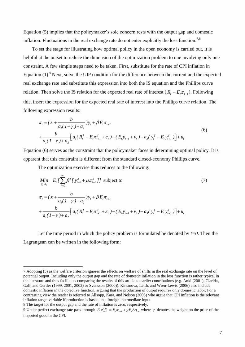
To set the stage for illustrating how optimal policy in the open economy is carried out, it is
helpful at the outset to reduce the dimension of the optimization problem to one involving only one
constraint. A few simple steps need to be taken. First, substitute for the rate of CPI inflation in
Equation (1).9
Next, solve the UIP condition for the difference between the current and the expected
real exchange rate and substitute this expression into both the IS equation and the Phillips curve
relation. Then solve the IS relation for the expected real rate of interest ( 1 ttt ER ). Following
this, insert the expression for the expected real rate of interest into the Phillips curve relation. The
following expression results:
t t t t 1
1 2
f f f f
1 t t t 1 t t t 1 t 3 t t t 1 t
1 2
b( )y E
a (1 ) a
ba ( R E ) ( E y v ) a ( y E y ) u
a (1 ) a
(6)
Equation (6) serves as the constraint that the policymaker faces in determining optimal policy. It is
apparent that this constraint is different from the standard closed-economy Phillips curve.
The optimization exercise thus reduces to the following:
t t
i 2 2
t t i t iy ,
i 0
Min E [ [ y ]]
subject to (7)
t t t t 1
1 2
f f f f
1 t t t 1 t t t 1 t 3 t t t 1 t
1 2
b( )y E
a (1 ) a
ba ( R E ) ( E y v ) a ( y E y ) u
a (1 ) a
Let the time period in which the policy problem is formulated be denoted by t=0. Then the
Lagrangean can be written in the following form:
7 Adopting (5) as the welfare criterion ignores the effects on welfare of shifts in the real exchange rate on the level of
potential output. Including only the output gap and the rate of domestic inflation in the loss function is rather typical in
the literature and thus facilitates comparing the results of this article to earlier contributions (e.g. Aoki (2001), Clarida,
Gali, and Gertler (1999, 2001, 2002) or Svensson (2000)). Kirsanova, Leith, and Wren-Lewis (2006) also include
domestic inflation in the objective function, arguing that the production of output requires only domestic labor. For a
contrasting view the reader is referred to Allsopp, Kara, and Nelson (2006) who argue that CPI inflation is the relevant
inflation target variable if production is based on a foreign intermediate input.
8 The target for the output gap and the rate of inflation is zero, respectively.
9 Under perfect exchange rate pass-through CPI
t t 1 t t 1 t t 1E E E q where denotes the weight on the price of the
imported good in the CPI.

8
2 2 2 2 2 2 2
0 0 0 1 1 2 2
f f
0 0 1 1 3 0 1 0 1 0 0 0
f f
1 1 2 2 3 1 2 1 1 1 1 1
2 f f
2 2 3 3 3 2 3 2 1 2 2 2
E [ y ( y ) ( y ) .....
(( c )y c( y a ( y y ) v a ) u )
(( c )y c( y a ( y y ) v a ) u )
(( c )y c( y a ( y y ) v a ) u ) ....
0M
.]
(8)
where f f
t t t t 1 tR E 1 2
bc
a (1 ) a
t 0,1,2,...
Taking the first-order conditions with respect to the two target variables in each time period yields
the following set of equations:
0 0
0
2y ( c ) 0y
0M (9)
1 0 1
1
2 y c ( c ) 0y
0M (10)
2 2
2 1 2
2
2 y c ( c ) 0y
0M (11)
…
…
0 0
0
2 0
0M (12)
1 0 1
1
2 0
0M (13)
2 1 2
2
2 0
0M (14)
…
…
The remainder of this section draws attention to the importance of a real exchange rate channel in
the Phillips curve and discusses its implication for optimal policymaking in an open economy
framework. Part A takes up the case where the real exchange rate channel is suppressed while part
B considers the case where the real exchange rate channel is operative. Part C analyzes the behavior
of the endogenous variables of the model and the policy instrument with the help of impulse
response functions.

9
A. No Real Exchange Rate Channel in the Phillips Curve: b=0
Setting b=0 implies c=0. Closer inspection of equations (9)-(11) then reveals that the first-
order condition for the output gap in each period establishes the same systematic relationship
between the output gap and the Lagrange multiplier:
t t2y 0 t = 0, 1, 2, 3,… (15)
The invariant optimizing condition for the output gap is used below to substitute for the Lagrange
multipliers to derive the optimal policy setting from a timeless perspective. Under this policy the
policymaker ignores the start-up condition for the rate of inflation. Only the systematic relationship
between the Lagrange multipliers and the rate of inflation from time t=1 onward is relevant:10
t t 1 t2 0 t = 1, 2, 3,… (16)
After using equation (15) to substitute for the Lagrange multipliers, one can express the target rule
under optimal policy from the timeless perspective as:
t t 1t
y y0
(17)
Thus in an open economy optimal policy from a timeless perspective is identical to optimal policy
in a closed economy provided that there is no real exchange rate channel in the Phillips curve. This
result is consistent with the observation by Clarida, Gali, and Gertler (2001), according to whom the
conduct of optimal policy in an open economy is isomorphic to policy in a closed economy.
B. A Real Exchange Rate Channel in the Phillips Curve: b>0
With the direct exchange rate channel being operative, the structure of the first-order
condition that applies to the output gap is no longer the same for all periods. More specifically, the
condition in the initial period is different from the one that obtains in succeeding periods. In this
respect the pattern followed by the output gap in the current context mirrors the pattern set by the
10 Equation (16) can also include the initial period, i.e. hold for t=0,1,2, 3…. In this case, to ensure dynamic
consistency, the rate of inflation should be set in accordance with this optimizing condition in every period. But a
special situation arises in the initial period. In period 0 the lagged Lagrange multiplier (λ-1) must equal zero. This
effectively rules out the Phillips curve in the previous period (t=-1) serving as a constraint in the optimization exercise
in period 0. Woodford (1999a,b), McCallum and Nelson (2004), Froyen and Guender (2007, Ch. 9) and Gali (2008,
Ch.5) provide a detailed analysis of optimal policy from a timeless perspective in a closed economy framework.
10
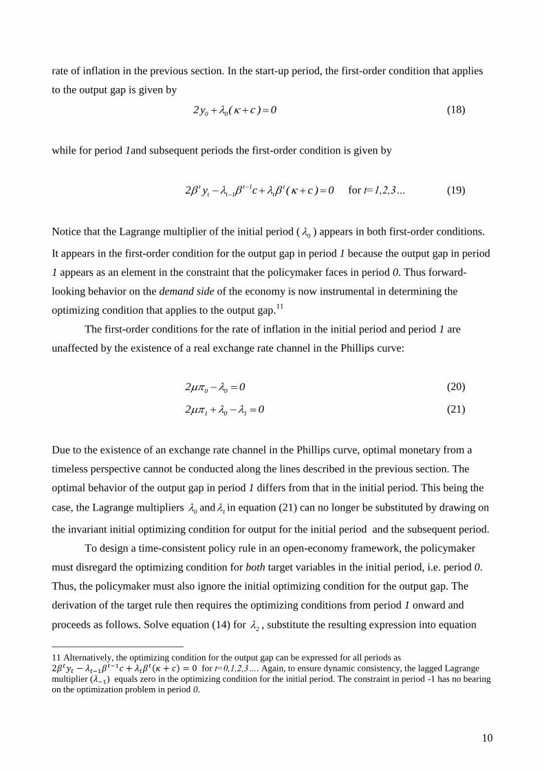
rate of inflation in the previous section. In the start-up period, the first-order condition that applies
to the output gap is given by
0 02y ( c ) 0 (18)
while for period 1and subsequent periods the first-order condition is given by
t t 1 t
t t 1 t2 y c ( c ) 0
for t=1,2,3… (19)
Notice that the Lagrange multiplier of the initial period (0 ) appears in both first-order conditions.
It appears in the first-order condition for the output gap in period 1 because the output gap in period
1 appears as an element in the constraint that the policymaker faces in period 0. Thus forward-
looking behavior on the demand side of the economy is now instrumental in determining the
optimizing condition that applies to the output gap.11
The first-order conditions for the rate of inflation in the initial period and period 1 are
unaffected by the existence of a real exchange rate channel in the Phillips curve:
0 02 0 (20)
1 0 12 0 (21)
Due to the existence of an exchange rate channel in the Phillips curve, optimal monetary from a
timeless perspective cannot be conducted along the lines described in the previous section. The
optimal behavior of the output gap in period 1 differs from that in the initial period. This being the
case, the Lagrange multipliers 0 and
1 in equation (21) can no longer be substituted by drawing on
the invariant initial optimizing condition for output for the initial period and the subsequent period.
To design a time-consistent policy rule in an open-economy framework, the policymaker
must disregard the optimizing condition for both target variables in the initial period, i.e. period 0.
Thus, the policymaker must also ignore the initial optimizing condition for the output gap. The
derivation of the target rule then requires the optimizing conditions from period 1 onward and
proceeds as follows. Solve equation (14) for 2 , substitute the resulting expression into equation
11 Alternatively, the optimizing condition for the output gap can be expressed for all periods as
for t=0,1,2,3…. Again, to ensure dynamic consistency, the lagged Lagrange
multiplier ( ) equals zero in the optimizing condition for the initial period. The constraint in period -1 has no bearing
on the optimization problem in period 0.
11
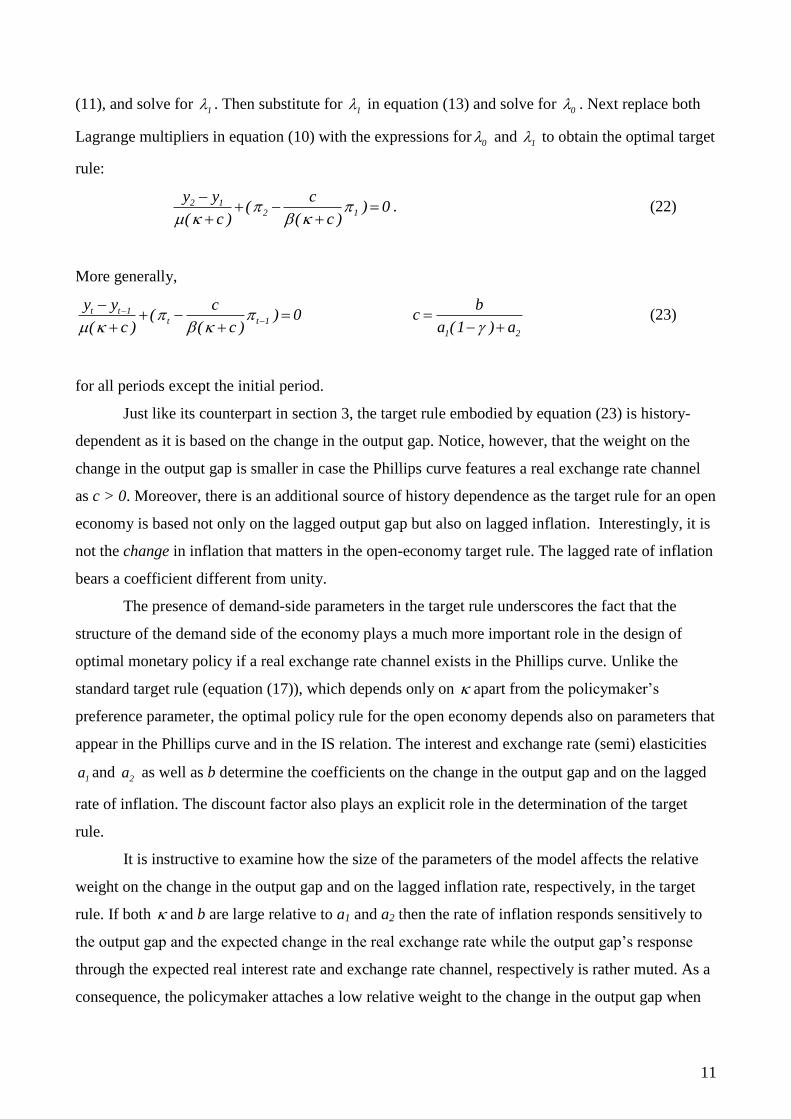
(11), and solve for 1 . Then substitute for
1 in equation (13) and solve for 0 . Next replace both
Lagrange multipliers in equation (10) with the expressions for0 and
1 to obtain the optimal target
rule:
2 12 1
y y c( ) 0
( c ) ( c )
. (22)
More generally,
t t 1t t 1
y y c( ) 0
( c ) ( c )
1 2
bc
a (1 ) a
(23)
for all periods except the initial period.
Just like its counterpart in section 3, the target rule embodied by equation (23) is history-
dependent as it is based on the change in the output gap. Notice, however, that the weight on the
change in the output gap is smaller in case the Phillips curve features a real exchange rate channel
as c > 0. Moreover, there is an additional source of history dependence as the target rule for an open
economy is based not only on the lagged output gap but also on lagged inflation. Interestingly, it is
not the change in inflation that matters in the open-economy target rule. The lagged rate of inflation
bears a coefficient different from unity.
The presence of demand-side parameters in the target rule underscores the fact that the
structure of the demand side of the economy plays a much more important role in the design of
optimal monetary policy if a real exchange rate channel exists in the Phillips curve. Unlike the
standard target rule (equation (17)), which depends only on apart from the policymaker‟s
preference parameter, the optimal policy rule for the open economy depends also on parameters that
appear in the Phillips curve and in the IS relation. The interest and exchange rate (semi) elasticities
1a and 2a as well as b determine the coefficients on the change in the output gap and on the lagged
rate of inflation. The discount factor also plays an explicit role in the determination of the target
rule.
It is instructive to examine how the size of the parameters of the model affects the relative
weight on the change in the output gap and on the lagged inflation rate, respectively, in the target
rule. If both and b are large relative to a1 and a2 then the rate of inflation responds sensitively to
the output gap and the expected change in the real exchange rate while the output gap‟s response
through the expected real interest rate and exchange rate channel, respectively is rather muted. As a
consequence, the policymaker attaches a low relative weight to the change in the output gap when

12
setting policy. Conversely, if a1 and a2 are large relative to and b then the relative weight on the
output gap in the target rule increases as the output gap reacts sensitively to the expected real
interest rate and an expected change in the real exchange rate. In this event, only a small increase in
the policy instrument is required to engineer a desired reduction in inflation through a contraction of
real output. The relative weight on lagged inflation decreases as well given the increased emphasis
on the output gap in setting policy.
The coefficient ( )
c
c measures the importance of lagged inflation in the target rule.
Lagged inflation enters the target rule because of the existence of an exchange rate channel in the
Phillips curve. The greater the sensitivity of the rate of inflation to expected changes in the real
exchange rate in the Phillips curve, i.e. the greater the size of b for given values of 1a ,
2a and ,
the more important the lagged rate of inflation becomes in setting policy today. Conversely, the
greater the sensitivity of the rate of inflation to the output gap in the Phillips curve, i.e. the greater
the size of for given values of 1a ,
2a , and b, the less significant the role of past inflation in the
target rule.
C. Why a Real Exchange Rate Channel in the Phillips Curve Matters
The importance of the real exchange rate channel for the behavior of the endogenous
variables of the model is brought out in Figures 1 – 4.12
These figures show how the output gap,
domestic inflation, the real exchange rate, and the nominal interest rate respond to a cost-push
shock, an IS shock, and a UIP shock.13
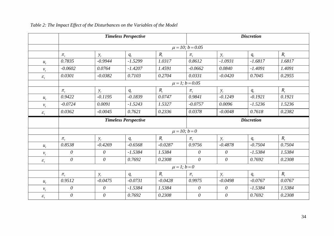
The quantitative impact effect of these shocks on the four
endogenous variables is also reported in Table 2.
Figure 1 depicts the response of the four variables to a positive cost-push shock when the
real exchange rate channel in the Phillips curve exists (b=0.05) while Figure 2 repeats the exercise
for the case when the real exchange rate does not exist (b=0).14
A comparison of the impulse
response functions of the two figures reveals that
12 All four figures are based on 10 . Table 1 lists the values of the parameters upon which the impulse response
analysis in this section is based. The table also lists the size of the variances of the shocks that figure in the comparisons
of policy under discretion and from a timeless perspective carried out in the next section.
13 The remaining shocks are only of minor interest as their effects are the same as or similar to a UIP or IS shock. For
instance, a foreign interest rate shock causes the same effect on the variables of interest as a UIP shock while a shock to
the foreign output gap behaves essentially like an IS shock.
14 So as to not overstate the importance of the real exchange rate channel relative to the output gap in the Phillips curve
b and are of the same size. In their study of six countries Guender and Yu (2007) find support for an exchange rate
channel in the Phillips curve only for Korea. The estimated size of b ranges from 0.04 to 0.1.

13
a positive cost-push shock has a much greater impact effect on the output gap, the real
exchange rate and the policy instrument if a real exchange rate channel exists in the Phillips
curve (b>0).
a positive cost-push shock has a somewhat greater impact effect on the rate of inflation if a
real exchange rate channel does not exist in the Phillips curve (b=0).
policy tightens in response to a positive cost-push shock if b > 0 according to Figure 1.
Notice the stark difference in Figure 2: choosing the optimal response to a cost-push shock,
the policymaker lowers the nominal interest rate if no real exchange rate channel exists in
the Phillips curve.
The intriguing behavior of the nominal interest rate can be traced to the UIP condition. The positive
cost- push shock causes the real exchange rate to fall, i.e. the right-hand side of the UIP condition
increases. At the same time, the positive cost-push shock lowers expected inflation next period
because of the decrease in the current output gap, thus also increasing the left-hand side of the UIP
condition.15
However, the reduction in the current output gap is sufficiently large to require a fall in
the nominal interest rate so that the UIP condition is restored in the aftermath of the cost-push
shock.16
Figure 3 shows that a domestic demand-side disturbance causes the rate of inflation and the
output gap to deviate from their respective target value. The top two panels illustrate how the rate of
inflation falls and the output gap rises in response to a positive IS shock for the case b=0.05.
According to the top panel of Table 2, these impact effects on inflation and the output gap are
quantitatively small, at -0.0574 and 0.0728, respectively. Nevertheless, they underscore the fact that
the policymaker is unable to prevent a one-time demand-side disturbance from affecting both target
variables temporarily. The responses of the policy instrument and the real exchange rate, which are
shown in the bottom panels, help explain why this is the case. In his effort to provide the optimal
stabilization response, the policymaker raises the nominal interest rate. The positive change in the
setting of the policy instrument causes the real value of the domestic currency to appreciate which
15 As shocks are white noise, expected inflation next period is given by: t t 1 20 t
E c y with
20c 0
16 Inspection of the reduced form equation for the output gap and the reaction function of the policymaker yields the
same insight. For b=0, 10 and values for the other parameters in accordance with Table 1, the two equations are:
t t 1 t
t t t 1 t
y 0.853893y 0.426946u
R 1.82519 y 1.50094 y 0.750496u
Substituting the former into the latter results in a negative coefficient on the cost-push shock. The nominal interest rate
decreases in the wake of a positive cost-push shock.
14
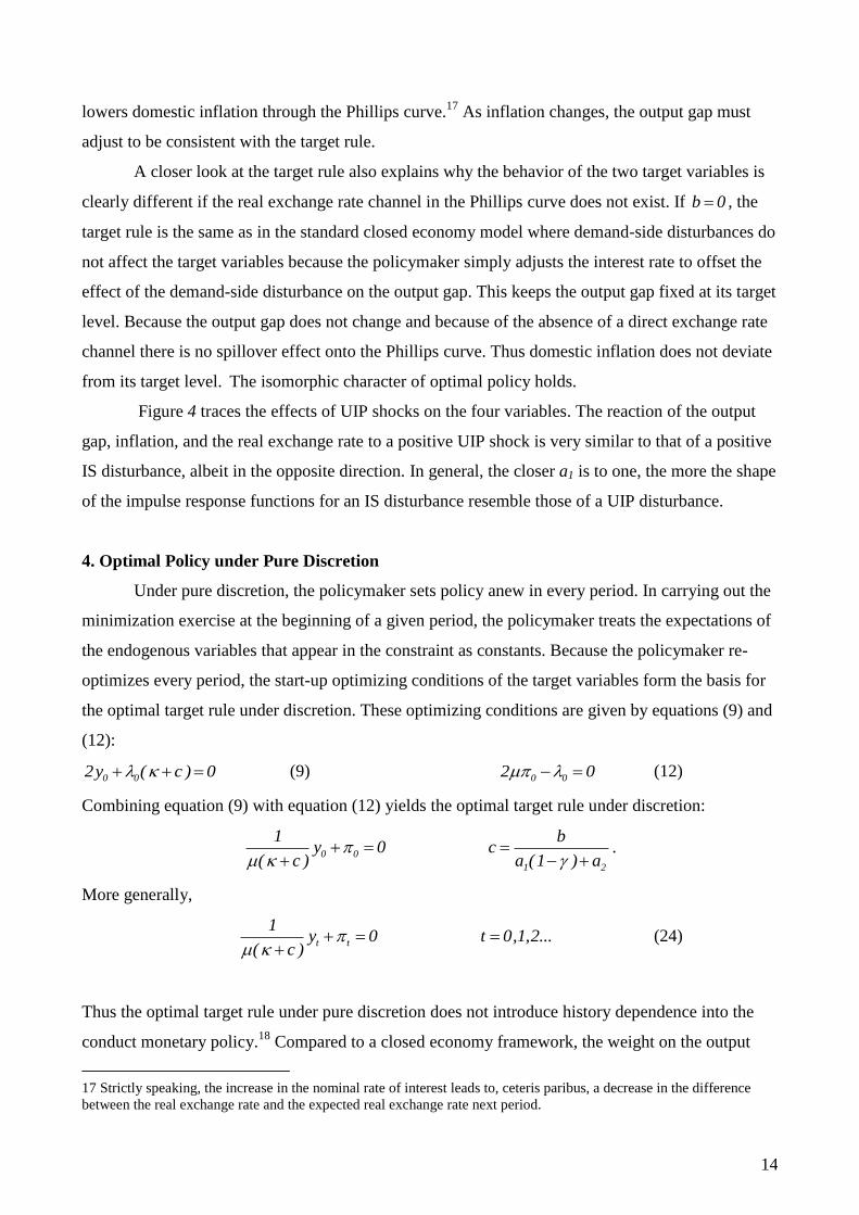
lowers domestic inflation through the Phillips curve.17
As inflation changes, the output gap must
adjust to be consistent with the target rule.
A closer look at the target rule also explains why the behavior of the two target variables is
clearly different if the real exchange rate channel in the Phillips curve does not exist. If b 0 , the
target rule is the same as in the standard closed economy model where demand-side disturbances do
not affect the target variables because the policymaker simply adjusts the interest rate to offset the
effect of the demand-side disturbance on the output gap. This keeps the output gap fixed at its target
level. Because the output gap does not change and because of the absence of a direct exchange rate
channel there is no spillover effect onto the Phillips curve. Thus domestic inflation does not deviate
from its target level. The isomorphic character of optimal policy holds.
Figure 4 traces the effects of UIP shocks on the four variables. The reaction of the output
gap, inflation, and the real exchange rate to a positive UIP shock is very similar to that of a positive
IS disturbance, albeit in the opposite direction. In general, the closer a1 is to one, the more the shape
of the impulse response functions for an IS disturbance resemble those of a UIP disturbance.
4. Optimal Policy under Pure Discretion
Under pure discretion, the policymaker sets policy anew in every period. In carrying out the
minimization exercise at the beginning of a given period, the policymaker treats the expectations of
the endogenous variables that appear in the constraint as constants. Because the policymaker re-
optimizes every period, the start-up optimizing conditions of the target variables form the basis for
the optimal target rule under discretion. These optimizing conditions are given by equations (9) and
(12):
0 02y ( c ) 0 (9) 0 02 0 (12)
Combining equation (9) with equation (12) yields the optimal target rule under discretion:
0 0
1 2
1 by 0 c
( c ) a (1 ) a
.
More generally,
t t
1y 0 t 0,1,2...
( c )
(24)
Thus the optimal target rule under pure discretion does not introduce history dependence into the
conduct monetary policy.18
Compared to a closed economy framework, the weight on the output
17 Strictly speaking, the increase in the nominal rate of interest leads to, ceteris paribus, a decrease in the difference
between the real exchange rate and the expected real exchange rate next period.

15
gap is smaller in an open economy provided that there is a real exchange rate channel in the Phillips
curve, i.e. c > 0.
5. An Evaluation of the Two Policy Regimes
In this section we compare and contrast the performance of optimal policy from a timeless
perspective relative to pure discretion in an open economy. To underscore the importance of a real
exchange rate channel in the Phillips curve for policymaking, we again distinguish between two
cases: b=0.05 and b=0. In addition, we employ two different values of the policymaker‟s relative
aversion to inflation variability: 1 and 10 .
Table 2 reports the coefficients on the three disturbances in the reduced form equations for
the rate of inflation, the output gap, the real exchange rate, and the nominal interest rate. The
coefficients in the top panel capture the contemporaneous response of the four variables to an IS
shock, a cost-push shock, and a UIP shock for the case where a real exchange rate channel is
operative in the Phillips curve: b=0.05. Inspection of these coefficients yields a few noteworthy
insights.
The impact effects of all three disturbances on the two target variablesty and
t are smaller
under policy from a timeless perspective than under discretion. This is a direct consequence
of the fact that commitment requires that the two target variables return gradually to their
target levels in the wake of a shock while discretion requires adjustment of the variables to a
shock within the period.
The impact effect (in absolute terms) of a cost-push disturbance on all four variables is
smaller under policy from a timeless perspective than discretion.
The picture is less clear for IS and UIP shocks. Suffice it to say that both shocks evoke
similar responses of the nominal rate of interest and the real exchange rate under both policy
strategies.
The lower panel reports results for the case where a real exchange rate channel in the
Phillips curve does not exist (b=0).
Here policy type matters for the reaction of the policy instrument in the face of a cost-push
shock as explained in the previous section.
In the absence of a real exchange rate channel in the Phillips curve, IS and UIP shocks have
no effect on the target variables under both forms of policy.
18 Examining the impulse response functions under discretion is not as revealing as under policy from a timeless
perspective. Because of the absence of history dependence under discretion, the effect of the shock is felt only in the
current period.

16
Both policy from a timeless perspective and discretion lead to the same contemporaneous
response of the real exchange rate and the nominal rate of interest, respectively, to IS and
UIP disturbances. This happens because the responses of both variables are independent of
policy design and thus purely mechanical.19
Table 3 summarizes the overall performance of the two policy strategies and reports the
variances of the three endogenous variables and the policy instrument for 1 and 10 . The top
panel considers the case where a real exchange rate channel is operative in the Phillips curve while
the bottom panel considers the case where it is absent. The dominance of policy under a timeless
perspective over discretion is evident. In all four cases expected losses under policy from a timeless
perspective are lower than under discretion. The gain from commitment relative to discretion does
vary, however, depending on whether a real exchange rate channel exists in the Phillips curve.
Substantial gains are realized in case the Phillips curve is the standard closed-economy variant.
Specifically, the percentage gain from commitment rises from 4.63 % to 12.47 % as the relative
weight on the variance of inflation in the expected loss function rises from 1 to 10. The
gain from commitment is more modest for an open-economy Phillips curve (b>0): as increases
from 1 to 10 the percentage gain from being able to precommit rises from 4.25 % to 9.02 %.
Overall, the policymaker wields better control over the variability of the rate of inflation if a
real exchange rate channel is operative in the Phillips curve. This comes at some cost though as the
variability of the output gap increases if b>0.
6. Is Price Level Targeting Consistent with Optimal Monetary Policy from a Timeless
Perspective in an Open Economy?
The presence of a real exchange rate channel in the Phillips curve has further implications
for policymaking in an open economy. This section shows why the delegation mechanism fails in
the open economy model proposed in this paper.
Woodford (1999a) argues that price level targeting is consistent with optimal policy from a
timeless perspective in the forward-looking model of a closed economy. This is a direct
consequence of the fact that price level targeting produces the same optimal response to
19 It is also worth pointing out that under discretion, the coefficient on the UIP shock in the reduced form equation for
the real exchange equals one minus the coefficient on the UIP shock in the equation for the nominal interest rate. This
result holds also under policy from a timeless perspective provided the real exchange rate channel in the Phillips curve
is not operative. The real exchange rate and the nominal rate of interest respond alike to an IS shock albeit in opposite
directions under discretion. This result also holds under commitment if b=0.

17
disturbances as policy from a timeless perspective. The literature on the delegation issue in the
conduct of monetary policy has recognized the attractiveness of price level targeting in the forward-
looking model.20
That price level targeting under discretion is compatible with optimal monetary
policy from a timeless perspective can be seen by comparing the target rules that underlie both
strategies of monetary policy.
In the standard New Keynesian framework, the target rule under optimal policy from a
timeless perspective relates the rate of inflation to the change in the output gap:
t t 1 t
1( y y ) 0
(25)
This target rule can be rewritten in terms of the output gap and the price level:21
t t
1y p 0
(26)
The target rule under discretionary price-level targeting is given by:22
t 22 t t 1t
y ( (1 ) 1) E yp 0
ˆ ˆ
(27)
The parameter denotes the weight the policymaker assigns to the squared deviations of the price
level from its target value in the intertemporal loss function. After replacing the expectation of the
output gap with 12 tp and some algebraic manipulation, we can restate equation (27) as:
23
22 tt
12
( (1 ) 1)yp 0
ˆ
(28)
Comparing (26) with (28), we find that the two target rules differ only to the extent of the relative
weight on the output gap. This in turn implies that in a closed-economy framework a suitably
chosen central banker who engages in discretionary price level targeting can replicate the behavior
of the rate of inflation and the output gap that occurs under optimal policy from a timeless
perspective.
20 See Vestin (2006) for an analysis of price level targeting and the delegation issue in the context of a closed economy.
21 In what follows we assume that the target for the price level (p*) is zero.
22 The derivation of the target rule under price level targeting is laid out in Appendix C.
23 12 = the coefficient on the lagged price level in the putative solution for the current price level.
22 = the coefficient
on the lagged price level in the putative solution for the current output gap.
18
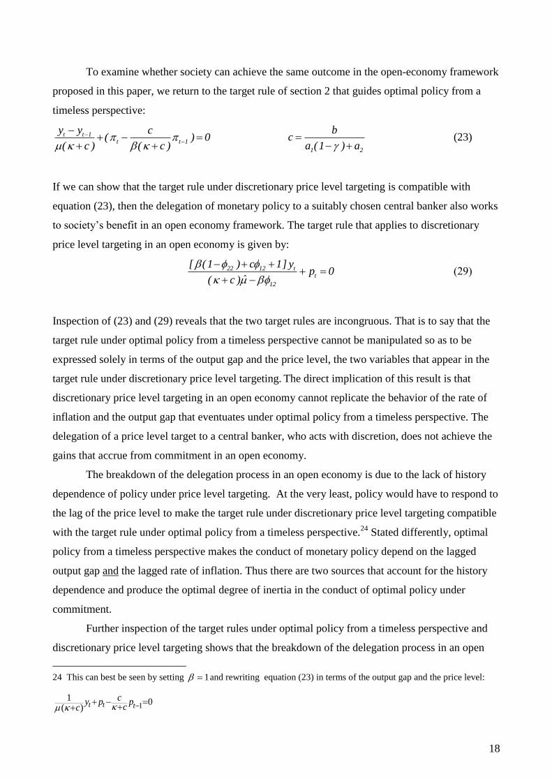
To examine whether society can achieve the same outcome in the open-economy framework
proposed in this paper, we return to the target rule of section 2 that guides optimal policy from a
timeless perspective:
t t 1t t 1
y y c( ) 0
( c ) ( c )
1 2
bc
a (1 ) a
(23)
If we can show that the target rule under discretionary price level targeting is compatible with
equation (23), then the delegation of monetary policy to a suitably chosen central banker also works
to society‟s benefit in an open economy framework. The target rule that applies to discretionary
price level targeting in an open economy is given by:
22 12 tt
12
[ (1 ) c 1] yp 0
ˆ( c )
(29)
Inspection of (23) and (29) reveals that the two target rules are incongruous. That is to say that the
target rule under optimal policy from a timeless perspective cannot be manipulated so as to be
expressed solely in terms of the output gap and the price level, the two variables that appear in the
target rule under discretionary price level targeting. The direct implication of this result is that
discretionary price level targeting in an open economy cannot replicate the behavior of the rate of
inflation and the output gap that eventuates under optimal policy from a timeless perspective. The
delegation of a price level target to a central banker, who acts with discretion, does not achieve the
gains that accrue from commitment in an open economy.
The breakdown of the delegation process in an open economy is due to the lack of history
dependence of policy under price level targeting. At the very least, policy would have to respond to
the lag of the price level to make the target rule under discretionary price level targeting compatible
with the target rule under optimal policy from a timeless perspective.24
Stated differently, optimal
policy from a timeless perspective makes the conduct of monetary policy depend on the lagged
output gap and the lagged rate of inflation. Thus there are two sources that account for the history
dependence and produce the optimal degree of inertia in the conduct of optimal policy under
commitment.
Further inspection of the target rules under optimal policy from a timeless perspective and
discretionary price level targeting shows that the breakdown of the delegation process in an open
24 This can best be seen by setting 1 and rewriting equation (23) in terms of the output gap and the price level:
11 0
( ) t t tcy p p
cc

19
economy framework is due to the existence of an exchange rate channel in the Phillips curve.
Setting b=0 yields c=0. Most important, the lagged rate of inflation drops out of the target rule
under optimal policy from a timeless perspective. This in turn restores the compatibility of
discretionary price level targeting with optimal policy from a timeless perspective.
7. Conclusion
This paper has examined the design of optimal monetary policy in an open economy version
of the forward-looking model. Its major finding is that the existence of a real exchange rate channel
in the Phillips curve changes the design of optimal policy in no small measure. First and foremost,
the target rule under policy from a timeless perspective becomes more complex. The lags of both
target variables appear in it, thus making the conduct of policy more history-dependent. The
discount factor as well as IS and Phillips curve parameters determine the weights attached to the
change in the output gap and the lagged rate of inflation.
With the target rule being significantly different if a real exchange rate channel is operative
in the Phillips curve, it is not surprising that the character of stabilization policy changes. The
policymaker can no longer perfectly stabilize both the domestic rate of inflation and the output gap
in the wake of IS or UIP disturbances by mechanically adjusting the policy instrument. Demand-
side disturbances thus cause temporary effects on both variables. Optimal stabilization policy in
such an open economy is no longer isomorphic to policy in a closed economy.
Whether or not a real exchange rate channel exists in the Phillips curve also matters for the
delegation issue. Discretionary price level targeting is consistent with optimal policy from a
timeless perspective in a closed economy because the target rules that govern both strategies are
compatible in the sense that they can be expressed in terms of the same target variables. This result
does not carry over to the open economy framework of this paper because the timeless perspective
introduces additional history dependence through inflation into the conduct of monetary policy.
This additional history dependence cannot be matched by price level targeting.
The paper also assesses the welfare gains under commitment relative to discretion. The
results suggest that the welfare gains under policy from a timeless perspective are somewhat lower
in an open economy framework where a real exchange rate channel exists in the Phillips curve.
Taken altogether, the findings reported in this paper warrant the conclusion that optimal
policy in an open economy framework is substantially different from optimal policy in a closed
economy. The mere existence of a real exchange rate channel in the Phillips curve suffices for the
conduct of optimal monetary policy from a timeless perspective to be more complex and
information-intensive. The realistic assumption that in a small open economy individual firms take

20
account of fluctuations in the terms of trade when adjusting prices provides a conduit through which
the real exchange rate enters the aggregate Phillips curve. Its presence there ensures a prominent
role for the real exchange rate in the design of optimal monetary policy.

21
References:
Allsopp, C., Kara A., and Nelson E. (2006). “UK Inflation Targeting and the Exchange Rate,”
Economic Journal, 116, 232-244.
Aoki, K. (2001). “Optimal Monetary Responses to Relative Price Changes,” Journal of Monetary
Economics, 48, 55-80.
Ball, L. (1999). "Policy Rules for Open Economies," In: Taylor J. B. (Ed.): Monetary Policy Rules,
University of Chicago Press, Chicago, 129-156.
-------- and Romer, D. (2003). “Inflation and the Informativeness of Prices,” Journal of Money,
Credit, and Banking 35, 177-196.
Bergin, P. and Feenstra, R. (2000). „Staggered Price Setting and Endogenous Persistence,‟ Journal
of Monetary Economics, vol. 45, 657-80.
Clarida, R., Gali, J.,. and Gertler, M. (1999). „The Science of Monetary Policy: a New Keynesian
Perspective,‟ Journal of Economic Literature, vol. 37, 1661-1707.
Clarida, R., Gali, J., and Gertler, M (2001). „Optimal Monetary Policy in Open vs. Closed
Economies: An Integrated Approach,‟ American Economic Review, vol. 91 (2001), 248-252.
Clarida, R., Gali, J., and Gertler, M. (2002). „A Simple Framework for International Monetary
Policy Analysis,‟ Journal of Monetary Economics, vol. 49, 879-904.
Dennis, R. (2001). „Optimal Policy in Rational Expectations Models: New Solution Algorithms,‟
mimeo, Federal Reserve Bank of San Francisco.
Froyen, R. and A. Guender, Optimal Monetary Policy under Uncertainty, Edward Elgar,
Cheltingham, 2008.
Gali, J. Monetary Policy, Inflation, and the Business Cycle, Princeton University Press, Princeton
and London, 2008.
Gali, J. and Monacelli, T. (2005). „Optimal Monetary Policy and Exchange Rate Volatility in a
Small Open Economy,‟ Review of Economic Studies, 72, 707-734.

22
Guender, A. (2006). “Stabilizing Properties of Discretionary Monetary Policies in a Small Open
Economy,” Economic Journal, 116, 309-326.
Guender, A. and Yu, X. (2007). “Is There an Exchange Rate Channel in the Forward-Looking
Phillips Curve? A Theoretical and Empirical Investigation,” New Zealand Economic Papers,
41 (1), 5-28.
Jensen, H. (2002). “Targeting Nominal Income Growth or Inflation?” American Economic Review,
92 (4), 928-956.
Kirsanova, T., Leith, C., and Wren-Lewis, S. (2006). “Should Central Banks Target Consumer
Prices or the Exchange Rate?” Economic Journal, 116, 208-231.
McCallum, B.T. and Nelson E. (2000). “Monetary Policy for an Open Economy: An Alternative
Framework with Optimizing Agents and Sticky Prices,” Oxford Review of Economic Policy,
16 (4), 74-91.
McCallum, B. T. and Nelson, E. (2004). “Timeless Perspective vs. Discretionary Monetary Policy
in Forward-Looking Models,” Federal Reserve Bank of St. Louis Review, 86, 2, 43-56.
Monacelli, T. (2005). “Monetary Policy in a Low Pass-Through Environment,” Journal of Money,
Credit, and Banking, 37 (6), 1047-1066.
Nessén, M. and Vestin, D. (2005). “Average Inflation Targeting”, Journal of Money, Credit, and
Banking, 37 (5), 837-863.
Roberts, J. M. (1995). „New Keynesian Economics and the Phillips Curve,‟ Journal of Money,
Credit, and Banking, vol. 27, 975-84.
Rotemberg, J. (1982). “Sticky Prices in the United States,” Journal of Political Economy, vol. 90,
1187-1211.
Soederstroem, U. (2005). “Targeting Inflation with a Role for Money,„ Economica, vol. 277, 577-
596.

23
Svensson, L. (2000). „Open Economy Inflation Targeting,‟ Journal of International Economics, vol.
50, 117-53.
Taylor J. B. (2000). „Low Inflation, Pass-Through, and the Pricing Power of Firms,‟ European
Economic Review, vol. 44 , 1389-1408.
Vestin, D. (2006). “Price-Level Targeting Versus Inflation Targeting,” Journal of Monetary
Economics 53 (7), 1361-1376.
Walsh, C. (1999). “Monetary Policy Tradeoffs in the Open Economy,” manuscript.
Walsh, C. (2003). “The Output Gap and Optimal Monetary Policy,” American Economic Review,
93 (1), 265-278.
Woodford, M. (1999a). “Commentary: How Should Monetary Policy Be Conducted in an Era of
Price Stability?” in New Challenges for Monetary Policy: A Symposium Sponsored by the
Federal Reserve Bank of Kansas City. Federal Reserve Bank of Kansas City, 277-316.
Woodford, M. (1999b). “Optimal Policy Inertia”, Manchester School 67 (Supplement), 1-35.

24
Appendix A: Derivation of the Open Economy Phillips Curve.
The starting point is Rotemberg (1982). Monopolistically competitive firms aim to minimize
menu costs weighed against the cost of being away from the optimal price they would charge in the
absence of those menu costs. This optimal price is denoted OPTp . In addition, being concerned
about changes in their competitiveness vis-à-vis foreign firms, domestic firms wish to avoid
changes in their terms of trade by engaging in terms-of-trade smoothing. Unstable terms of trade
interfere with the domestic firms‟ competitiveness in the domestic market as well as world markets.
Such fluctuations tend to unhinge the steady market share of firms. Specifically, at time t domestic
firms attempt to minimize the squared difference between the current and next period‟s terms of
trade.25
The objective function faced by the typical firm j is:
t
2 2i OPT 2
t t t i t i t i t i 1 t 1 i t ip( j )
i 0
min ( j ) E p( j ) p( j ) c p( j ) p( j ) d( q( j ) q( j ) )
(A1)
where:1
t( j ) = the total cost of firm j at time t
tp( j ) = the price of the good produced by firm j at time t
OPT
tp( j ) = the optimal price firm j charges
f
t t t tq( j ) p s p( j ) = firm-specific terms of trade
= the constant discount factor
c = the parameter that measures the costs of changing prices relative to the costs of
deviating from the optimal price
d = the parameter that measures the costs of changes in the firm‟s terms of trade relative
to the costs of deviating from the optimal price
tE = the expectations operator conditional on information available at time t.
After taking and rearranging the first-order condition for the above cost-minimization
problem, we can characterize the relationship between past, current, and future price levels as well
as the current and expected terms of trade as:
OPT
t t 1 t t 1 t t t t t 1 t
1 dp ( j ) p( j ) E p( j ) p( j ) p( j ) p( j ) ( E q( j ) q( j ) )
c c (A2)
25 Alternatively, the firm could be concerned about minimizing the deviation between t i
q
and t i 1
q
in which case the
first-order condition would contain the change in the current firm-specific terms of trade next to the change in the
expected terms of trade. The resulting Phillips curve would then also feature the change in the real exchange rate (t
q
t 1q
). Including , while defensible, complicates the analysis considerably as it rules out the derivation of an
analytical target rule that lends itself to straightforward interpretation. For this reason, this case is not pursued here.

25
Here we see that the expected change in the firm-specific terms of trade matters in the pricing
decision. The greater the relative weight of expected changes in the terms of trade in the total cost
function compared to the relative weight on costly price changes, the more the expected change in
the terms of trade factors in the decision to change the price of output in the current period. Changes
in the current nominal exchange rate and changes in the price charged by competing foreign firms
are beyond the control of the typical domestic firm – they are exogenous. Yet such changes affect
its terms of trade, i.e. its competitiveness. The only way that a domestic firm can counteract such
pressure is to adjust its domestic price in such a way so that overall costs are minimized.
Next, consider the formation of the firm‟s optimal price:
OPT
t t t tˆp( j ) p y( j ) ( j ) 0 (A3)
where all variables are as previously defined. In addition:
tp = the price charged by competing firms at time t
ty( j ) = output produced (relative to potential) by firm j
t( j ) = a stochastic disturbance.
Under imperfect competition, a firm sets its optimal price as a mark-up over marginal cost.
But marginal cost and real output are positively related.26
Hence it is innocuous to replace marginal
cost with the output gap in (A3). To capture the idea of a time-varying mark-up factor, we treat it as
a random element that enters into the process of setting the optimal price. Hence t appears in
equation (A3).27
The other important factor that influences the firm‟s optimal price is the benchmark price set
by competing firms. This price, denoted by,tp equals the aggregate domestic price level
tp .
Substituting equation (A3) into (A2) and aggregating over all firms yields equation (A4), an
open-economy Phillips curve:
t t t 1 t t t t 1 tE y b( q E q ) u (A4)
where
26 Within a general equilibrium framework, the co-movement between marginal cost and economic activity can be
established by combining the labor supply and demand relations with the market clearing condition in the goods market.
On this point see Clarida, Gali, and Gertler (2001, 2002) or Gali and Monacelli (2005) who derive a similar relation that
stresses the positive relation between real marginal cost and domestic consumption. The positive link between output
and marginal cost is also characteristic of earlier models of monopolistic competition such as Blanchard and Kiyotaki
(1987). The link features also prominently in Mankiw and Reis (2002) who propose an alternative Phillips curve that is
based on slow dissemination of information.
27 For an investigation of the time-varying mark-up factor, see Ball and Romer (2003).
26
1 ttt pp
ttttt ppEE 11
c
d
bc
tt
cu
1 .
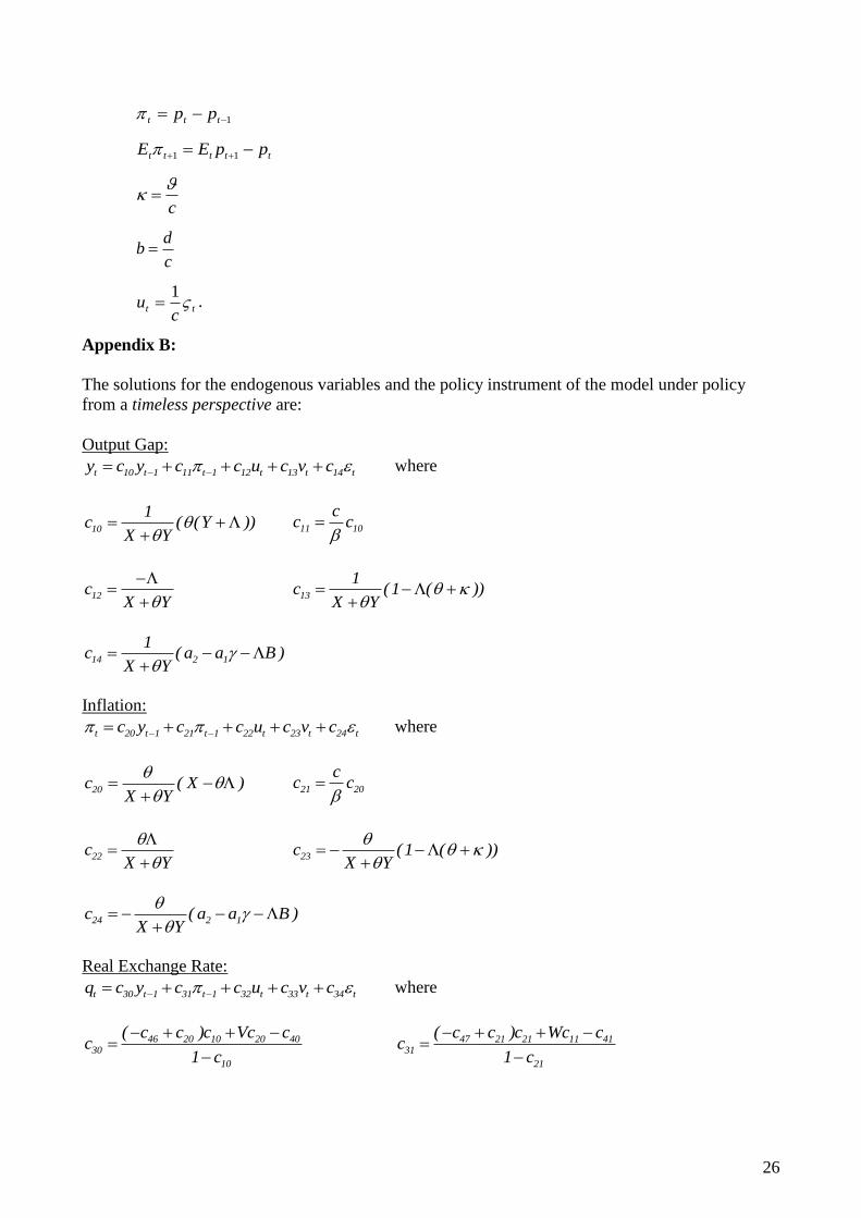
Appendix B:
The solutions for the endogenous variables and the policy instrument of the model under policy
from a timeless perspective are:
Output Gap:
t 10 t 1 11 t 1 12 t 13 t 14 ty c y c c u c v c where
10
1c ( (Y ))
X Y
11 10
cc c
12cX Y
13
1c (1 ( ))
X Y
14 2 1
1c ( a a B )
X Y
Inflation:
t 20 t 1 21 t 1 22 t 23 t 24 tc y c c u c v c where
20c ( X )X Y
21 20
cc c
22cX Y
23c (1 ( ))X Y
24 2 1c ( a a B )X Y
Real Exchange Rate:
t 30 t 1 31 t 1 32 t 33 t 34 tq c y c c u c v c where
46 20 10 20 4030
10
( c c )c Vc cc
1 c
47 21 21 11 41
31
21
( c c )c Wc cc
1 c

27
32 12 22 42 33 13 23 43
34 14 24 44
c Wc Vc c c Wc Vc c
c Wc Vc (1 c )
Nominal Interest Rate:
t 40 t 1 41 t 1 42 t 43 t 44 tR c y c c u c v c where
40 46 10 47 20c c c c cA
41 46 11 47 21
cc c c c c
A
42 46 12 47 22c c c c cA
43 46 13 47 23
( )c c c c c
A
44 46 14 47 24
Bc c c c c
A
46 10 20c ( )c ( 1)cA A
47 11 21c ( )c ( 1)cA A
1 2 2 1A (1 )a a B b ( )( a a )
A 1 bc
( )A b ( c ) A
11 11 21Y c (( )c c ) 10 10 20X 1 ( c (( )c c ))
30 46 20 31 47 21W c c c V c c c
The solutions for the endogenous variables and the policy instrument of the model under Discretion
are:
Output Gap:
t t t 1 t
1y ( Au bv a b )
D
Inflation:
t t t 1 t( Au bv a b )D
Real Exchange Rate:
1t 1 t t t
a b1 Aq (( a ) (( )v u ))
A D D
Nominal Interest Rate:
1t 2 1 t t t
a b1 AR (( a a ) (( )v u ))
A D D
where D b A( )

28
Appendix C:
Under discretionary price-level targeting, the policymaker minimizes the current and
expected future deviations of the price level and the output gap from its respective target value. The
minimization exercise is repeated every period and the process of expectations formation is taken as
given. The constraint for the policy problem is obtained by combining the UIP condition and the IS
relation with the Phillips curve.
t t
j 2 * 2
t t j t jy ,p j 0
t t t 1 t t t 1
f f f f
1 t t t 1 t t t 1 t 3 t t t 1 t
ˆMin E ( y ( p p ) )
1s.t. p [ E p ( c )y u p
1
c( a ( R E ) ( E y v ) a ( y E y )) u ]
(C1)
= policymaker‟s aversion to price level variability.
Taking the first-order conditions with respect to the choice variables ty and
tp yields:
tt
( c )2y 0
1
(C2)
* t t 1t t 22 12
E1ˆ2 ( p p ) [ ( c ) 1] 0
1 1
(C3)
Notice that the conditional expectations of the price level and the output gap in period t+1 have
been replaced with the conditional expectation of the respective putative solution. The
undetermined coefficients 12 and
22 appear in the putative solution for the output gap and the
price level, respectively:
11 12 1 13 14 15 16 17
f f f
t t t t t t t ty u p v R y (C4)
21 22 1 23 24 25 26 27
f f f
t t t t t t t tp u p v R y (C5)
Combining the first-order conditions (and setting *p 0 ) results in the target rule that
systematically relates the price level to the current and the expected output gap in period t+1.
t 22 12 t t 1t
y ( (1 ) c 1) E yp 0
ˆ ˆ( c ) ( c )
(C6)
Letting 1 12t t tE y p and rearranging the above equation yields the target rule under price level
targeting in the text (Equation (29)). Equation (27) obtains if c 0 , i.e. if the real exchange rate
channel in the Phillips curve does not exist.

29
Figure 1:

30
Figure 2:

31
Figure 3:

32
Figure 4:
33
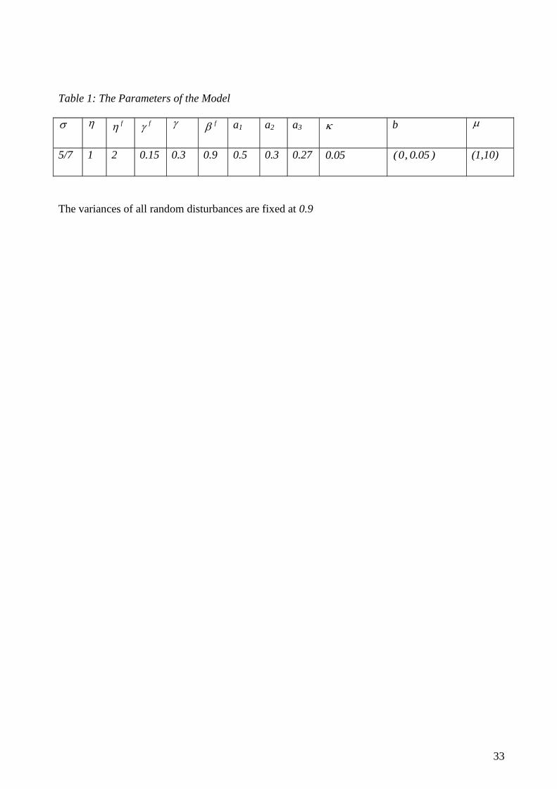
Table 1: The Parameters of the Model
f f f a1 a2 a3 b
5/7 1 2 0.15 0.3 0.9 0.5 0.3 0.27 0.05 (0, 0.05 ) (1,10)
The variances of all random disturbances are fixed at 0.9
34
Table 2: The Impact Effect of the Disturbances on the Variables of the Model
Timeless Perspective
Discretion
10; b 0.05
t
ty tq
tR t
ty tq
tR
tu 0.7835 -0.9944 -1.5299 1.0317 0.8612 -1.0931 -1.6817 1.6817
tv -0.0602 0.0764 -1.4207 1.4591 -0.0662 0.0840 -1.4091 1.4091
t 0.0301 -0.0382 0.7103 0.2704 0.0331 -0.0420 0.7045 0.2955
1; b 0.05
t ty tq tR t ty tq tR
tu 0.9422 -0.1195 -0.1839 0.0747 0.9841 -0.1249 -0.1921 0.1921
tv -0.0724 0.0091 -1.5243 1.5327 -0.0757 0.0096 -1.5236 1.5236
t 0.0362 -0.0045 0.7621 0.2336 0.0378 -0.0048 0.7618 0.2382
Timeless Perspective
Discretion
10; b 0
t ty tq tR t ty tq tR
tu 0.8538 -0.4269 -0.6568 -0.0287 0.9756 -0.4878 -0.7504 0.7504
tv 0 0 -1.5384 1.5384 0 0 -1.5384 1.5384
t 0 0 0.7692 0.2308 0 0 0.7692 0.2308
1; b 0
t ty tq tR t ty tq tR
tu 0.9512 -0.0475 -0.0731 -0.0428 0.9975 -0.0498 -0.0767 0.0767
tv 0 0 -1.5384 1.5384 0 0 -1.5384 1.5384
t 0 0 0.7692 0.2308 0 0 0.7692 0.2308

35
Table 3: Summary Measures of the Performance of Commitment and Discretion
b=0.05 Timeless Perspective Discretion
10
tV( ) tV( y ) tV( q ) tV( R ) tV( ) tV( y )
tV( q ) tV( R )
0.5985 1.1188 4.9035 2.9454 0.6725 1.0834 4.7791 4.4109
% Gain from Commitment: 9.02
1
tV( ) tV( y ) tV( q ) tV( R ) tV( ) tV( y ) tV( q ) tV( R )
0.8250 0.0293 2.6830 2.1840 0.8781 0.0141 2.6450 2.1737
% Gain from Commitment: 4.25
b=0 Timeless Perspective Discretion
10
tV( ) tV( y ) tV( q ) tV( R ) tV( ) tV( y ) tV( q ) tV( R )
0.7079 0.6056 4.0962 2.1808 0.8566 0.2141 3.1696 2.6849
% Gain from Commitment: 12.47
1
tV( ) tV( y ) tV( q ) tV( R ) tV( ) tV( y ) tV( q ) tV( R )
0.8347 0.02139 2.7133 2.1954 0.8955 0.0022 2.6680 2.1834
% Gain from Commitment: 4.63
Notes: Expected Loss = S S S
t t tE( L V( y ) V( )) S=TP or D Gain from Commitment:
D TP
t t
D
t
E( L ) E( L )x100
E( L )
1. The above loss function obtains after premultiplying the intertemporal loss function by (1 ) and letting 1.
2. Only the variances of the cost-push shock, IS shock, and the UIP shock enter into the calculation of the variances of inflation, the output gap, the real exchange rate,
and the policy instrument.