Optimal Design of Water Distribution Networks under

Optimal Design of Water Distribution Networks under Uncertainty

by

Seyed Abdolnaser Moosavian

A THESIS SUBMITTED IN PARTIAL FULFILLMENT OF

THE REQUIREMENTS FOR THE DEGREE OF

DOCTOR OF PHILOSOPHY

in

THE FACULTY OF GRADUATE AND POSTDOCTORAL STUDIES

(Civil Engineering)

THE UNIVERSITY OF BRITISH COLUMBIA

(Vancouver)

November 2018

© Seyed Abdolnaser Moosavian, 2018

ii

The following individuals certify that they have read, and recommend to the Faculty of

Graduate and Postdoctoral Studies for acceptance, the dissertation entitled:

Optimal design of water distribution networks under uncertainty

submitted by The student in partial fulfillment of the requirements for

the degree of Doctor of Philosophy

in Civil Engineering

Examining Committee:

Barbara J. Lence, Civil Engineering

Supervisor

Ziad K. Shawwash, Civil Engineering

Supervisory Committee Member

Steven Weijs, Civil Engineering


W Scott Dunbar, Mining Engineering

University Examiner

Jose Marti, Electrical and Computer Engineering

University Examiner

Additional Supervisory Committee Members:



iii

Abstract

Generally, the use of the water distribution network (WDN) modeling is divided into two main

categories, WDN design, and WDN hydraulic analysis, which itself is employed as part of WDN

design. The former generally identifies components of the network, considering the system cost

and the ability of the network to satisfy consumer demands for water availability, pressure, and

quality. The latter evaluates the distribution of nodal pressures and pipe flows under a specified

network design and known or estimated water consumption levels. WDN analysis is often

embedded within design algorithms, where, for every potential design considered, the hydraulic

energy and continuity equations that govern the system are solved. If water demands and the

physical characteristics of the network design are known with certainty, deterministic approaches

for solving these equations may be used. If some information is uncertain, non-deterministic

approaches are used for identifying the Probability Density Function or the fuzzy membership

functions of the pressure and flow conditions at all locations in the network.

This dissertation is divided into three main parts, 1) the application and development of

evolutionary algorithms for single- and multi-objective optimization of WDNs, 2) the introduction

of new frameworks and performance surrogates as objectives in the optimization of WDNs, and

3) the advancement of an efficient gradient-based technique for fuzzy analysis of WDNs under

uncertainty. First, efficient Evolutionary Algorithms (EAs) are compared and advanced for

reducing the computational burden of single- and multi-objective design of WDNs, respectively.

We investigate and identify the most appropriate operators and characteristics of EAs for

optimization of realistic-sized networks. Based on the experiences and capabilities of EAs

obtained, a new EA is introduced for single-objective optimization of WDNs which is faster and

more reliable than other popular algorithms presented in the literature. Next, two different

frameworks are introduced for implementing many objectives in the optimization of realistic-sized

WDNs. Both approaches can distinguish appropriate design solutions with minimum cost and

maximum hydraulic and mechanical reliability. Finally, a fuzzy method is introduced for analysis

of WDNs under uncertainty. The proposed technique significantly reduces the CPU time of

uncertainty analysis of large-scale networks.

iv

Lay Summary

Water distribution projects that provide drinking water for municipalities are among the most

expensive of installed infrastructure. These systems include many components and thousands of

junctions and pipes, connected together for transmission of water. They are usually constructed in

a loop-shape to minimize the risk of failing to supply water at all demand sites when one or many

pipes have been removed for scheduled repair, or unexpectedly broken due to pipe decay or high

pressures. There are many uncertain conditions in these systems, including consumption levels,

pipe age and operability. Design and maintenance of these systems requires consideration of many

details and plans to respond to abnormal circumstances. This dissertation develops techniques to

improve the quality of the designs of these systems by minimizing cost and maximizing reliability.

This work may be used to undertake appropriate simulation and optimization of designs before

construction and implementation of these systems.

v

Preface

Chapter 2 is published in the Canadian Journal of Civil Engineering (CSCE); I have conducted all

the testing, computational analysis and wrote most of the manuscript. Dr. Lence edited all spelling

the manuscript and directed the arrangements and presenting the results. This paper is:

Moosavian N., Lence B., Testing evolutionary algorithms for optimization of water distribution

networks, Canadian Journal of Civil Engineering (CSCE), (2018). Canadian Journal of Civil

Engineering, https://doi.org/10.1139/cjce-2018-0137

Chapter 3 is published in the ASCE Journal of Water Resources Planning and Management. I

conducted the computational analysis and wrote 70% of the manuscript. Dr. Lence revised the

manuscript, and directed the development of methods for analyzing the results and frameworks for

presenting these. This paper is:

Moosavian N., Lence B.J., Nondominated sorting differential algorithms for multi-objective

optimization of water distribution systems, Journal of Water Resources Management and Planning

(ASCE), (2016). http://ascelibrary.org/doi/abs/10.1061/(ASCE)WR.1943-5452.0000741

Chapter 4 is based on a submitted journal paper; I have conducted the testing, computational

analysis and wrote most of the manuscript. Dr. Lence edited the manuscript and directed the

additions of conceptual proofs of the algorithm developed, as well as the testing of the algorithm,

and directed the arrangements and presenting of the results.

Chapter 5 is published in the ASCE Journal of Water Resources Planning and Management. Dr.

Lence, Hanieh Daliri and I suggested the initial idea related to the application of the game theory

in the area of multi-objective optimization of WDNs. I developed the fuzzy programming idea and

conducted the computational analysis, provided the results and wrote 50% of the manuscript. Dr.

Lence wrote 50% of the document and directed the computational work, and Hanieh Daliri

conducted literature review. This paper is:

Lence B.J., Moosavian N., Daliri H., A fuzzy programming approach for multi-objective

optimization of water distribution systems, Journal of Water Resources Management and Planning

(ASCE), (2017). http://ascelibrary.org/doi/abs/10.1061/(ASCE)WR.1943-5452.0000769

vi

Chapter 6 is based on a submitted journal paper. I proposed the initial idea and conducted

computational analysis and Dr. Lence developed the methodology and the results sections and

revised the manuscript.

Chapter 7 has been published in the ASCE Journal of Hydraulics. I proposed the idea, conducted

computational analysis and wrote the 80% of the paper. Dr. Lence revised the manuscript and

directed the presentation of the results. This paper is:

Moosavian N., Lence B. J., Fuzzy analysis of water distribution networks, Journal of Hydraulic

Engineering, (ASCE), (2018). DOI: 10.1061/(ASCE)HY.1943-7900.0001483

vii

Table of Contents

Abstract .......................................................................................................................................... iii

Lay Summary ................................................................................................................................. iv

Preface ............................................................................................................................................. v

Table of Contents .......................................................................................................................... vii

List of Tables ................................................................................................................................. xi

List of Figures .............................................................................................................................. xiii

List of Abbreviations .................................................................................................................... xv

List of Symbols ........................................................................................................................... xvii

Acknowledgments...................................................................................................................... xxiii

Dedication .................................................................................................................................. xxiv

Chapter 1 : Introduction .................................................................................................................. 1

1.1 Introduction ...................................................................................................................... 1

1.2 Research Questions and Guide to the Reader .................................................................. 6

1.2.1 Published Work .............................................................................................................. 6

1.2.2 Summary ......................................................................................................................... 8

1.3 Literature Review .................................................................................................................. 8

1.3.1 WDN Design .................................................................................................................. 8

1.3.2 WDN Hydraulic Analysis ............................................................................................. 12

1.5 Example Networks .............................................................................................................. 19

1.5.1 Two-loop network ........................................................................................................ 19

1.5.2 Hanoi network .............................................................................................................. 19

1.5.3 NewYork network ........................................................................................................ 19

1.5.4 Farhadgerd network ...................................................................................................... 20

1.5.5 Nagpur network ............................................................................................................ 20

1.5.6 EXNET network ........................................................................................................... 20

1.5.7 Hypothetical networks .................................................................................................. 21

1.6 Summary ............................................................................................................................. 21

Chapter 2 : Testing Evolutionary Algorithms for Optimization of Water Distribution Networks 39

2.1 Preface ................................................................................................................................. 39

2.2 Abstract ............................................................................................................................... 39

2.3 Introduction ......................................................................................................................... 40

viii

2.4 Problem formulation ........................................................................................................... 42

2.5 Evolutionary Algorithms (EAs) .......................................................................................... 44

2.5.1 Genetic Algorithm (GA) ............................................................................................... 44

2.5.3 Harmony Search (HS) .................................................................................................. 46

2.5.4 Differential Evolution (DE) .......................................................................................... 46

2.5.5 Particle Swarm Optimization and Gravitational Search Algorithm (PSOGSA) .......... 47

2.5.6 Artificial Bee Colony (ABC) ........................................................................................ 48

2.5.7 Soccer League Competition (SLC) Algorithm ............................................................. 49

2.5.8 Covariance Matrix Adaptation Evolution Strategy (CMAES) ..................................... 49

2.5.9 MEtaheuristics for Systems Biology and BIoinformatics Global Optimization (MEIGO) ............................................................................................................................... 50

2.5.10 Whale Optimization Algorithm (WOA) ..................................................................... 51

2.6 Applications to WDN design .............................................................................................. 52

2.6.1 Two-loop benchmark network...................................................................................... 52

2.6.2 Hanoi benchmark network ............................................................................................ 53

2.6.3 Farhadgerd network ...................................................................................................... 54

2.7 The Friedman test ................................................................................................................ 55

2.8 Conclusion ........................................................................................................................... 55

Chapter 3 : Nondominated Sorting Differential Evolution Algorithms for Multi-Objective Optimization of Water Distribution Systems ................................................................................ 71

3.1 Preface ................................................................................................................................. 71

3.2 Abstract ............................................................................................................................... 71

3.3 Introduction ......................................................................................................................... 72

3.4 Cost and Reliability in Water Distribution Systems (WDSs) ............................................. 74

3.5 Differential Evolution Algorithms for Multi-Objective Design of WDSs .......................... 76

3.5.1 Differential Evolution (DE) .......................................................................................... 76

3.5.2 Nondominated Sorting Differential Evolution (NSDE) ............................................... 78

3.5.3 Nondominated Sorting Differential Evolution with Ranking-based Mutation (NSDE-RMO) ..................................................................................................................................... 78

3.6 Multi-objective Design of WDSs ........................................................................................ 79

3.7 Benchmark and Experimental Networks ............................................................................. 79

3.8 Performance of Multi-objective Optimization Algorithms ................................................. 81

3.9 Conclusion ........................................................................................................................... 83

ix

Chapter 4 : Fittest Individual Referenced Differential Evolution Algorithm for Optimization of Water Distribution Networks ........................................................................................................ 99

4.1 Preface ................................................................................................................................. 99

4.2 Abstract ............................................................................................................................... 99

4.3 Introduction ....................................................................................................................... 100

4.4 Differential Evolution (DE) and Fittest Individual Referenced Differential Evolution (FDE) Algorithms ................................................................................................................... 104

4.5 Sensitivity Analysis and Performance of FDE for EA Benchmark Test Problems .......... 107

4.6 Water Distribution Network (WDN) Design Problem Formulation ................................. 109

4.7 Differential Evolution Algorithms for Design of WDNs .................................................. 110

4.7.1 Application of FDE for Benchmark Networks ........................................................... 111

4.7.2 Application of FDE for Farhadgerd WDN ................................................................. 113

4.8 Discussion and Conclusion ............................................................................................... 115

Chapter 5 : A Fuzzy Programming Approach for Multi-Objective Optimization of Water Distribution Systems ................................................................................................................... 139

5.1 Preface ............................................................................................................................... 139

5.2 Abstract ............................................................................................................................. 139

5.3 Introduction ....................................................................................................................... 140

5.4 Fuzzy Programming for Multi-objective Optimization of Cost and Reliability ............... 143

5.5 Multi-objective Optimization of Water Distribution Systems (WDSs) ............................ 145

5.6 Soccer League Competition (SLC) Algorithm .................................................................. 148

5.7 Fuzzy Multi-objective Optimization of the Farhadgard WDS .......................................... 149

5.7.1 Hydraulic Reliability .................................................................................................. 150

5.7.2 Mechanical Reliability ................................................................................................ 151

5.7.3 Comparison with Compromise Set Ideal Solution ..................................................... 152

5.8 Conclusions ....................................................................................................................... 153

Chapter 6 : Flow Uniformity Index for Reliable-Based Optimal Design of Water Distribution Networks ..................................................................................................................................... 165

6.1 Preface ............................................................................................................................... 165

6.2 Abstract ............................................................................................................................. 165

6.3 Introduction ....................................................................................................................... 166

6.4 The Uniformity Index ........................................................................................................ 168

6.5 Multi-objective Optimization Model ................................................................................ 170

6.5.1 Minimize the total system cost ................................................................................... 170

x

6.5.2 Maximize resilience, Ir ............................................................................................... 171

6.5.3 Maximize uniformity, Iu , or Eq. (6.1) ........................................................................ 171

6.6 Multi-objective Optimization Algorithm .......................................................................... 172

6.7 Multi-objective Optimal WDN Designs ........................................................................... 173

6.7.1 Farhadgerd Network ................................................................................................... 174

6.8 Conclusion ......................................................................................................................... 177

Chapter 7 : Approximation of Fuzzy Membership Functions in Water Distribution Network Analysis....................................................................................................................................... 190

7.1 Preface ............................................................................................................................... 190

7.2 Abstract ............................................................................................................................. 190

7.3 Introduction ....................................................................................................................... 191

7.4 Co-Content Model for WDN Analysis.............................................................................. 194

7.5 Relationships for Demands, Pipe Resistance and Nodal Pressures .................................. 195

7.6 Fuzzy Analysis of WDNs .................................................................................................. 197

7.7 Examples ........................................................................................................................... 198

7.7.1 Nagpur Medium-Sized Network ................................................................................ 198

7.7.2 Hypothetical Large-Sized Network ............................................................................ 199

7.8 Conclusion ......................................................................................................................... 199

Chapter 8 : Conclusions .............................................................................................................. 208

8.1 Summary of thesis objectives and methodologies ............................................................ 208

8.2 Research conducted ........................................................................................................... 208

8.2.1 Development of EAs for single- and multi-objective optimization of WDNs ........... 208

8.2.2 Development of a new framework and introduction of new surrogates for improving the quality of WDN design .................................................................................................. 209

8.2.3 Advancement of numerical methods for Fuzzy Analysis of WDNs .......................... 210

8.3 Suggestions for future work .............................................................................................. 210

8.3.1 Application of efficient optimization algorithms for multi-objective WDN design .. 210

8.3.2 Applications of new surrogates in reliability-based optimization of WDNs .............. 211

8.3.3 Development of Fuzzy-reliability concept for WDN design under uncertainty ........ 211

Bibliography ............................................................................................................................... 213

Appendices .................................................................................................................................. 231

Appendix A. The FDE code for minimization of the Sphere Function in Python .................. 231

Appendix B Pipe and nodal information for Farhadgerd network .......................................... 233

xi

List of Tables

Table 1.1 Candidate pipe size diameters and corresponding costs for Two-loop network .......... 22 Table 1.2 Nodal information for Two-loop network .................................................................... 23 Table 1.3 Pipe information for Two-loop network ....................................................................... 24 Table 1.4 Candidate pipe size diameter and corresponding costs for Hanoi network .................. 25 Table 1.5 Hydraulic data for Hanoi network ................................................................................ 26 Table 1.6 Candidate pipe size diameter and corresponding costs for New York network ........... 27 Table 1.7 Hydraulic data for New York tunnel network .............................................................. 28 Table 1.8 Candidate pipe size diameter and corresponding costs for Farhadgerd network ......... 29 Table 1.9 Nodal information for Farhadgerd network .................................................................. 30 Table 1.10 Pipe characteristics for Farhadgerd network .............................................................. 31

Table 2.1 Least cost solutions for the Two-loop network: 1000 function evaluations ................. 58 Table 2.2 Least cost solutions for the Two-loop network: 10000 function evaluations ............... 59 Table 2.3 Least cost solutions for the Two-loop network: 40000 function evaluation ................ 60 Table 2.4 Least cost solutions for the Hanoi network: 1000 function evaluations ....................... 61 Table 2.5 Least cost solutions for the Hanoi network: 10000 function evaluations ..................... 62 Table 2.6 Least cost solutions for the Hanoi network: 40000 function evaluations ..................... 63 Table 2.7 Least cost solutions for the Farhadgerd network: 1,000 function evaluations ............. 64 Table 2.8 Least cost solutions for the Farhadgerd network: 10,000 function evaluations ........... 65 Table 2.9 Least cost solutions for the Farhadgerd network: 40,000 function evaluations ........... 66

Table 3.1 Average of twenty executions of the algorithms .......................................................... 85

Table 4.1 DE and FDE Algorithms for solving optimization problems ..................................... 117 Table 4.2 Initial population for f(x,y)=x2+y2 EA benchmark test problem ............................... 118 Table 4.3 First iteration of DE and FDE for optimization of f(x,y)= x2+y2 EA benchmark test problem ....................................................................................................................................... 119 Table 4.4 Second iteration of DE and FDE for optimization of the benchmark problem .......... 120 Table 4.5 EA benchmark test problems ...................................................................................... 121 Table 4.6 Sensitivity analysis based on EA benchmark test problem ........................................ 122 Table 4.7 Relevant optimization model information for three benchmark networks ................. 123 Table 4.8 Optimization results obtained based on different EAs and meta-heuristic algorithms for Two-loop network ....................................................................................................................... 124 Table 4.9 Optimization results obtained based on different EAs and meta-heuristic algorithms for Hanoi network ............................................................................................................................. 125 Table 4.10 Optimization results obtained based on different EAs and meta-heuristic algorithms for New York Tunnels network .................................................................................................. 127 Table 4.11 parameter values of ten EAs ..................................................................................... 129 Table 4.12 Least cost solutions for the Farhadgerd network: 1000 function evaluations .......... 130 Table 4.13 Least cost solutions for the Farhadgerd network: 10,000 function evaluations ....... 131 Table 4.14 Least cost solutions for the Farhadgerd network: 40,000 function evaluations ....... 132

xii

Table 4.15 Optimization results obtained based on different EAs and meta-heuristic algorithms for Farhadgerd network............................................................................................................... 133

Table 5.1 Fuzzy Multi-objective WDN Solutions for Town of Farhadgerd ............................... 155 Table 5.2 Cut-set Analyses of Fuzzy Multi-objective WDN Solutions for Town of Farhadgerd..................................................................................................................................................... 156 Table 5.3 Cut-set Analyses of Fuzzy Multi-objective WDN Solutions with 10% Increase in Demands ..................................................................................................................................... 157 Table 5.4 Compromise WDN Solution, with α = 2, for Town of Farhadgerd ............................ 158 Table 5.5 Cut-set Analysis of Compromise WDN Solution, with α = 2, for Town of Farhadgerd..................................................................................................................................................... 159

Table 6.1 Design diameters and pipe failure head losses for single loop network ..................... 179 Table 6.2 Cut-set analysis for Farhadgerd network with zero-meter pressure target, minimize-cost-maximize- Ir model ............................................................................................................. 180 Table 6.3 Cut-set analysis for Farhadgerd network with 20-meter pressure target, minimize-cost-maximize- Ir model ..................................................................................................................... 181 Table 6.4 Cut-set analysis for Farhadgerd network with zero-meter pressure target, minimize-cost-maximize- Ir -maximize- Iu model ..................................................................................... 182 Table 6.5 Cut-set analysis for Farhadgerd network with 20-meter pressure target, minimize-cost-maximize- Ir -maximize- Iu model .............................................................................................. 183 Table 6.6 Least cost designs for cut-set analysis accommodating 60-64 pipe removals for Farhadgerd network .................................................................................................................... 184 Table 6.7 Minimum pressure and location for a 10% increase in nodal demands for Farhadgerd network, least cost designs .......................................................................................................... 185

Table 7.1 The comparison of different methods for Fuzzy analysis of the networks ................. 201

xiii

List of Figures

Figure 1.1 WDN modeling framework ......................................................................................... 32 Figure 1.2 Two-loop network ....................................................................................................... 33 Figure 1.3 Hanoi network ............................................................................................................. 34 Figure 1.4 New York tunnel network ........................................................................................... 35 Figure 1.5 Farhadgerd network ..................................................................................................... 36 Figure 1.6 Nagpur network ........................................................................................................... 37 Figure 1.7 EXNET network .......................................................................................................... 38 Figure 2.1 Two-loop network ................................................................................................................. 67 Figure 2.2 Hanoi network ............................................................................................................. 68 Figure 2.3 Farhadgerd network ..................................................................................................... 69 Figure 2.4 Results of Friedman test for: a) 1,000, b) 10,000, and c) 40,000 function evaluations of three networks........................................................................................................................... 70 Figure 3.1 Pareto optimal front of Two-loop network ........................................................................ 86 Figure 3.2 Pareto optimal front of Hanoi network ........................................................................ 87 Figure 3.3 Pareto optimal front of Farhadgerd network ............................................................... 88 Figure 3.4 Pareto optimal front for WDN 100x200, 100 nodes and 200 pipes ............................ 89 Figure 3.5 Pareto optimal front for WDN 200x400, 200 nodes and 400 pipes ............................ 90 Figure 3.6 Pareto optimal front for WDN 400x800, 400 nodes and 800 pipes ............................ 91 Figure 3.7 IGD at each generation for Two-loop network ........................................................... 92 Figure 3.8 IGD at each generation for Hanoi network ................................................................. 93 Figure 3.9 IGD at each generation for Farhadgerd network ......................................................... 94 Figure 3.10 IGD at each generation for WDN100x200 ................................................................ 95 Figure 3.11 IGD at each generation for WDN200x400 ................................................................ 96 Figure 3.12 IGD at each generation for WDN400x800 ................................................................ 97 Figure 4.1 Conceptualization of mutation operation for DE and FDE ........................................... 134 Figure 4.2 Initial solution vectors for f(x,y)=x2+y2 EA benchmark test problem ..................... 135

Figure 4.3 EA benchmark test problems ..................................................................................... 136 Figure 4.4 Convergence properties of DE and FDE for EA benchmark test problems, based on two-variable formulations ........................................................................................................... 137 Figure 4.5 Convergence properties of DE and FDE for EA benchmark test problems, based on ten-variable formulations .................................................................................................................. 138 Figure 5.1 Water-main network of Farhadgerd, Iran ......................................................................... 160 Figure 5.2 Design diameter for the fuzzy Cost+Ir and Cost+NRI models ................................. 161 Figure 5.3 Design diameter for the fuzzy Cost+Ir and Cost+Id models ..................................... 162 Figure 5.4 Design diameter for the fuzzy Cost+Ir+Id and Cost+NRI+Id models ...................... 163 Figure 6.1 Uniform flow single loop network, WDN(a), (b) Non-uniform flow single loop network, WDN(b) ................................................................................................................................... 186

xiv

Figure 6.2 Pareto-optimal frontier for Farhadgerd network ............................................................. 187 Figure 6.3 Pareto-optimal frontier for Farhadgerd network considering cost and Ir, based on (a) minimize-cost-maximize- Ir -maximize- Iu model, (b) minimize-cost-maximize- Ir , (c) both models ...................................................................................................................................................... 188 Figure 6.4 Diameter distribution for Farhadgerd network, least cost solutions for the pipe cut-set with (a) Zero-meter pressure target, minimize-cost-maximize-Ir model, (b) Zero-meter pressure target, minimize-cost-maximize-Ir-maximize-Iu model, (c) 20-meter pressure target, minimize-cost-maximize-Ir model, (d) 20-meter pressure target, minimize-cost-maximize-Ir-maximize-Iu model ................................................................................................................................................... 189 Figure 7.1 Nagpur network ................................................................................................................... 202 Figure 7.2 Fuzzy membership functions for H1, H10, H20, H30, H40, H50, H60, H70, H80, H90, H100, H110, H120, H130, and H140 obtained by the three fuzzy hydraulic analysis approaches ............................................................................................................................................... 204 Figure 7.3 EXNET network .................................................................................................................. 205 Figure 7.4 Fuzzy membership functions for H100, H200, H300, H400, H500, H600, H700, H800, H900, H1000, H1100, H1200, H1300, H1500, and H1800, with 10% and 20% variability of nodal demands, obtained by Gupta and Bhave, and the proposed method ................................ 207

xv

List of Abbreviations

ABC = Artificial Bee Colony

ACO = Ant Colony Optimization

CMAES = Covariance Matrix Adaptation Evolutionary Strategy

DE = Differential Evolution

EA = Evolutionary Algorithm

FDE = Fast Differential Evolution

FORM = First Order Reliability Analysis

GA = Genetic Algorithm

GGA = Global Gradient Algorithm

HS = Harmony Search

INLP = Integer Nonlinear Programming

ILP = Integer Linear Programming

LP = Linear Programming

MCS = Monte-Carlo Simulation

MEIGO = MEtaheuristics for Systems Biology and BIoinformatics Global Optimization

MF = Membership Function

NLP = Nonlinear Programming

NSDE = Nondominated Sorting Differential Evolution

NSGA = Nondominated Sorting Genetic Algorithm

PDF = Probability Density Function

PSO = Particle Swarm Optimization

PSOGSA = Particle Swarm Optimization Gravitational Search Algorithm

SA = Simulated Annealing

xvi

SLC = Soccer League Competition

SQP = Sequential Quadratic Programming

WDN = Water Distribution Network

WOA = Whale Optimization Algorithm

xvii

List of Symbols

Related to the Chapter 2

Dk = diameter of pipe k;

kk Dc = cost of pipe k per unit length with diameter Dk;

Lk = length of pipe k;

Hj = pressure at node j;

ℎ𝑓 = head loss due to friction in the pipe k;

𝑛𝑙 = number of loops;

nn = number of nodes in the network;

np = number of pipes in the network;

ns = number of candidate diameters;

Qk = flow of pipe k;

qj = demand at node j;

𝑅 = resistance coefficient of the pipe k;

∆𝐻 = difference between nodal pressures at both ends of a path.


C = cost;

CH = Hazen-Williams coefficient;

CP = penalty;

CR = crossover rate;

D = diameter of pipe;

F = mutation scale factor;

L = length of pipe;

H = head pressure at node;

xviii

H0 = elevation head of a reservoir;

Hmin = minimum pressure head required;

hf = head loss;

Ir = resilience index;

nl = number of loops;

nn = number of nodes;

np = number of pipes;

no = number of reservoirs;

NPOP = number of population;

P = pump;

Pr = probability of selection;

Q = flow in pipe;

q = nodal demand;

Rank = rank of each solution in the population;

S = number of candidate diameters;

sn = random integer number;

X = solution vectors;

γ = specific weight of water;

λ = penalty multiplier.


C = cost;


CP = penalty;

CR = crossover rate;

xix


F = mutation scale factor;

L = length of pipe;

H = head pressure at node;



hf = head loss;





NPOP = number of population;

Pr = probability of selection;

Q = flow in pipe;

q = nodal demand;

ns = number of candidate diameters;

X = solution vectors;

Xbest = best solution vector;


λ = penalty multiplier.


C = cost;


dα = minimum distance to the ideal solution;

xx


H = pressure head at node;



hf = head loss;


Is = minimum surplus head index;

Id = diameter uniformity index;

L = length of pipe;

nk = number of pipes connected to node k;





NRI = network resilience index;

P = pump;

Q = flow in pipe;

q = nodal demand;

Zkk* = ideal solution for objective kk;

Zkk(x) = optimal solution for objective kk;

α = metric between one and infinity;


µ = fuzzy membership function;

λ = auxiliary decision variable.

xxi


C = cost;



H = pressure head at node;



hf = head loss;


Iu = flow uniformity index;

L = length of pipe;

nkin = number of pipes with flows that enter the node ;

nkout = number of pipes with flows that exit the node;





Q = flow in pipe;

q = nodal demand;

𝑄𝑘𝑖𝑛 = flow in pipe kin which is entering the node;

𝑄𝑘𝑜𝑢𝑡 = flow in pipe kout which is exiting the node.


CC = co-content model;

Ek = energy loss in pipe k;

xxii

Hj = pressure at node j;

hk = head loss in pipe k;

Qk = flow of pipe k;

qj = demand at node j;

𝑅 = resistance coefficient of the pipe k.

xxiii

Acknowledgments

I would like to express my sincere gratitude to my supervisor, Dr. Barbara Lence, for her

motivation, thoughtful advice, and continuous support. Her guidance helped me in all the time of

research and writing of this thesis. Dr. Lence, thank you very much for your trust on me in these

three years.

Besides, I would like to thank the rest of my thesis committee, Dr. Ziad Shawwash, Dr. Scott

Dunbar, Dr. Jose Marti, Dr. Steven Weijs and Dr. Holger Maier for their time and insightful

comments regarding the review of my dissertation.

Sincere appreciation goes to my father, Rahim, my mother, Homa, and my brother, Hashem, for

encouraging me in this period.

Last but not the least, I would like to thank the person who has always stood by my side, the reason

of my pride, the one who has provided me with her continuous love and support, to the love of my

life, my wonderful wife, Hanieh.

This work was supported by UBC’s Four Year Doctoral Fellowship.

xxiv

Dedication

To my wife, Hanieh

1

Chapter 1 : Introduction

1.1 Introduction

Next to air, water is the most indispensable element required for human survival. Municipalities

classify water uses as domestic, public, commercial, and industrial. Domestic uses include water

required for drinking, cooking, bathing, washing, heating, cooling, air-conditioning, sanitary

purposes, private swimming pools, and watering lawns and gardens. Public uses include water

needed for public places and buildings such as parks and fountains, public gardens and swimming

pools, hospitals, universities and other educational institutions, prisons, public sanitary places,

street and sewer flushing, and firefighting. Commercial uses include water for hotels and

restaurants, office buildings, car washes, laundries, shopping centres, bus and railway terminals,

and airports. Industrial uses are typically for manufacturing and processing, including heat

exchange and cooling (Bhave and Gupta 2006). For all classifications, water transmission lines

and pipe networks are employed to convey large amounts of water to demand and consumption

sites. The optimal design of water distribution network (WDNs) is often considered a least-cost

optimization problem with pipe sizes for commercially available pipes being the primary discrete

decision variables. The total cost is a function of the pipe design diameters and material, and the

diameters in turn affect the network pressures. The main requirement of the problem is to satisfy

minimum desired pressures at all network nodes. For each design solution, estimation of the

pressure level at all consumption nodes requires the simultaneous solution of nonlinear energy and

linear flow equations for the entire network, which significantly complicates the design problem.

During the design optimization process, considering uncertain parameters such as nodal

consumptions, further increases the complexity of the problem.

The first underground pipe network for water distribution is located in Knosis on the Island of

Crete, and is 2500 years old. The first public water system was constructed in 700 BC when sloped

hillside tunnels, called Qanats, were built to transport water in Persia. In 312 BC, Romans began

to construct aqueducts. The first public water supply system in the United States was installed in

1652 AD when the City of Boston incorporated its water works to provide water for fire-fighting

and domestic use. The first municipal water pumping station in Canada was installed in Toronto

by 1841. Since then many public water supply systems have been installed (Ormsbee 2006).

2

The US Environmental Protection Agency (EPA), in the fifth report on drinking water

infrastructure (2013), stated that a total of $384.2 billion US is required in water infrastructure

investments over the next 20 years, 64.4% of which, is needed for the transmission and

distribution. Thus, it is essential that the water infrastructure functions properly to ensure the

continuous supply of safe water with the required quality and pressures.

Generally, the use of WDN modelling is divided into two main categories, WDN design, and WDN

hydraulic analysis, which itself is employed as part of WDN design. The WDN design generally

selects elements of the system, such as pipe diameters and configurations, and pump and valve

characteristics, considering the system cost and the capability of the network to satisfy consumer

demands for water availability, pressure, and quality. WDN hydraulic analysis estimates the

distribution of nodal pressures and pipe flow under a specified network design and known or

probable water consumption levels.

This thesis investigates the application of single- and multi-objective optimization algorithms and

fuzzy programming formulations for WDN design, and introduces a new algorithm for identifying,

and a new surrogate for improving, design solutions. An efficient numerical technique for fuzzy

analysis to accommodate uncertainty is also developed.

Figure 1.1 provides the modelling framework for the design and analysis of WDNs, including how

and where uncertainty may be addressed. The optimization of WDN designs may be divided into

methods that formulate the problem as having a single or multiple objectives. In the single-

objective models, the problem has only one main goal (such as to minimize network cost) as the

objective function. Other minor goals can be considered as constraints. In the multi-objective

models, the problem has more than one main goal (such as minimize cost and maximize reliability

indices), and evaluates all objectives as important. Examples of methods for undertaking WDN

design are shown in the figure. Given the discrete nature of the decision variables (e.g.,

commercially available diameters of pipes), early applications of optimization to this problem used

continuous and integer formulations of classical mathematical techniques. Given their

computational power and ability to overcome the limitations of classical methods, heuristic

approaches, such as Evolutionary Algorithms (EAs), have been increasingly applied, and are

currently considered a standard techniques for solving this problem.

3

Under optimization models that minimize network cost, the best set of pipe size diameters is

selected to assure that required pressure at all nodes in the network is satisfied. In the literature,

this single-objective optimization problem is considered to be a nonlinear, non-convex, NP-hard

problem, and is one of the most well-known benchmark problems for testing the performance of

different heuristic algorithms. The earliest version of a Genetic Algorithm (GA) also was tested in

a single-objective gas pipeline optimization problem by Goldberg (1983). The complexity of this

problem is mainly related to the hydraulics of the network. For each design solution, hydraulic

analysis is undertaken to calculate the amount and direction of flows in pipes and the pressures at

all nodes. Since different solution designs have different pipe flow directions and values, finding

the global optimum solution is difficult using classical optimization algorithms. Therefore, only

powerful algorithms with specific exploration properties are capable of efficiently solving this

problem. In Chapter 2, the investigation of convergence characteristics and efficiency of ten

popular EAs is undertaken for the single-objective design of three pipe networks. Some of these

algorithms are tested and analyzed for the first time, and when compared with other popular EAs,

show promise for rapid convergence to the global optimum. Such efficient EAs may be suitable

alternatives in the design of large-sized WDNs with thousands of pipes and nodes.

Generally, design optimization of WDNs faces more than one objective. For example, to identify

robust network designs, reliability and resilience surrogates are estimated and integrated in

constraints or objectives to improve the quality of the optimal design in the face of hydraulic

uncertainty and pipe failures. When considered as objectives in multi-objective models,

populations of solutions with different values of objective functions are evaluated and the Pareto

optimal frontier for these objectives is investigated. There are many multi-objective EAs for

determining the Pareto frontier effectively. In Chapter 3, the investigation of convergence

characteristics and efficiency of four popular nondominated sorting EAs, including the

nondominated sorting genetic (NSGA_II) and nondominated sorting differential evolution

(NSDE) algorithms and variations of these, are undertaken for the multi-objective design of a wide

range of networks. In the WDN design model, one objective is minimization of cost function and

another objective is maximization of a reliability index. The NSDE algorithm with ranking based

mutation is applied for optimization of the multi-objective WDN design model for the first time in

this chapter, and results show that this algorithm can effectively find the optimal Pareto frontier

and has the highest convergence rate. These results, and the simple structure of the differential

4

evolution (DE) algorithm and coding process inspired the author to develop an improved DE

algorithm for WDN optimization. Chapter 4 presents a modified DE algorithm which adds the

most effective characteristics of other EAs and is highly effective for solving single-objective

WDN design problems. The proposed algorithm is implemented for optimization of three popular

benchmark problems and the Farhadgerd City WDN in Iran, and compared with other EAs for

WDN design.

In recent years, the ability of networks to satisfy water demands under normal and abnormal

operating conditions, including during pipe bursts and as components deteriorate, has been defined

in terms of hydraulic and mechanical reliability of the system. Hydraulic reliability is a

representative measure of the ability of the system to respond to gradual changes in the system

characteristics, e.g., available pipe diameters and pipe roughness, and short- or long-term shifts in

consumption, e.g., hourly variations in withdrawal rates or community-driven changes in required

fire flows. Mechanical reliability is a measure of the ability of the system to adapt to mechanical

failures, e.g., to maintain operating goals during pipe, valve, or pump failures.

For enhancing both mechanical and hydraulic reliability in WDN design, researchers propose

several reliability surrogates and apply these individually and in combination to improve WDN

design solutions. Chapter 5 proposes a fuzzy multi-objective programming model for combining

these surrogates in the optimal design of WDNs. Unlike the nondominated sorting-based multi-

objective models in Chapter 3, which provide populations of solutions on the Pareto optimal

frontier, the fuzzy programming model converges to only one good compromise solution.

While effective at identifying solutions that exhibit hydraulic reliability, the above-mentioned

surrogates may be inaccurate measures of network reliability in the face of mechanical failures. In

Chapter 6, a flow uniformity index is proposed to address this limitation. The uniformity index

may be considered as a surrogate for mechanical reliability, i.e., increasing it generally improves

mechanical reliability of a system. For all pipes and nodes in the network, the scaled ratios of

input (and output) pipe flows to the total input (and output) pipe flows are evaluated. The

uniformity index is the minimum of these ratios among all pipes at each node, and among all nodes

in the network. For each node, the scaling factor for each input (or output) pipe is equivalent to the

number of input (output) pipes for that node. The use of scaling factors reduces the dependence on

network configuration, resulting in an indicator that describes the degree of uniformity at each

5

node in the system, the minimum of which is the least amount of uniformity at any node in the

system. The index can be used to compare the uniformity of different designs of a single network

configuration, or of different configurations. The maximization of the uniformity index leads to a

network design with increasingly uniform flows throughout, where the burden of flow conveyance

is shared more evenly among all input (or output) pipes, and where the surplus hydraulic power is

gradually decreased from the supply reservoir(s) to the extremes of the network.

WDN hydraulic analysis is generally embedded within design algorithms, where, for every

potential design considered, the hydraulic energy and continuity equations that govern the system

must be solved. If input parameters such as water demands are known with certainty, deterministic

approaches for solving these equations may be used. If this information is uncertain, non-

deterministic approaches are used for approximating the measures of performance under uncertain

conditions. In non-deterministic analyses, the aforementioned input parameters do not have

certain values. Rather, Probability Theory may be used to identify Probability Density Functions

(PDFs) for quantifiable parameter and Fuzzy Set Theory is used to identify Fuzzy Membership

(FM) functions for linguistic parameters. There are several methods for non-deterministic analysis

such as Monte-Carlo Simulation for incorporating both Probability and Fuzzy Set Theory,

Reliability Analysis for incorporating Probability Theory, and Fuzzy Analysis techniques for

incorporating Fuzzy set theory. The main advantage of the application of Fuzzy Set Theory is the

simple construction of the FMs for variables that can only be described linguistically. This

technique can identify the extreme values of unknown variables when uncertain input information

ranges between pre-specified extremes, and when the PDFs of the information cannot be obtained.

The FMs help the designer to estimate the worst conditions for providing the sufficient amount of

water in the network facing nodal consumption variations, and provide useful insight toward

making decisions for avoiding these conditions. There are two main approaches for conducting the

Fuzzy Analysis in WDN design: 1) optimization methods and 2) gradient-based methods. The

optimization methods are very time-consuming processes which need many hydraulic analyses for

constructing the MFs. The initial applications of the gradient-based method improves the

efficiency of Fuzzy Analyses for middle-sized networks. However, this method is not readily

applicable for large-sized networks. Approximations of the gradients of the equations that govern

WDN analysis, with respect to nodal demands and pipe resistance, are identified in Chapter 7 and

harnessed to accelerate Fuzzy Analysis of system hydraulics.

6

1.2 Research Questions and Guide to the Reader

This thesis is a published paper-based document. The research centers on seeking answers to eight

questions.

(i) How do evolutionary algorithms (EAs) perform when applied for single-objective design and

optimization of WDNs?;

(ii) How do EAs perform when applied for multi-objective design and optimization of WDNs?;

(iii) Can one apply fuzzy programming to develop a framework for addressing more than two

objectives in design and optimization of WDNs?;

(iv) How should several reliability surrogates for identifying appropriate design solutions of

WDNs be integrated in the design and optimization of WDNs?;

(v) How can flow distribution in networks influence the design quality?:

(vi) How should fuzzy set theory for hydraulic analysis of large-scale WDNs under uncertainty be

advanced?: and

(vii) How should advanced numerical techniques for fuzzy analysis of pipe networks be developed

to reduce the computational burden?;

1.2.1 Published Work

Generally, this thesis investigates issues related to pipe network analysis and design. Four chapters

of this research are published and two chapters have been submitted and are currently being peer-

reviewed for publication. A brief explanation of the thesis contributions to the literature includes:

EAs Applied to Single-Objective WDN Design: to address some portions of Research Question

(i), in Chapter 2, ten evolutionary algorithms are tested for optimal single-objective design of

WDNs. Here, the objective function is the total cost of the network and the main constraint is the

satisfaction of minimum required pressure head at all nodal demand sites. An early form of this

work, testing only 6 algorithms, was presented at the Canadian Society of Civil Engineering

Conference (Moosavian and Lence 2017), and the full Journal Paper has been published in the

Canadian Journal of Civil Engineering, (Moosavian and Lence 2018).

EAs Applied to Multi-Objective WDN Design: to address Research Question (ii), in Chapter 3,

four efficient evolutionary algorithms are tested for optimal multi-objective design of WDNs.

7

Here, the objectives are minimization of the total cost of the network and maximization of the

resilience index proposed by (Todini 2000). This work demonstrates that by slightly modifying

the Differential Evolution (DE) algorithm, the speed of convergence of the algorithm is improved

for large-scale networks. The paper related to this chapter has been published as a Technical Paper

in the ASCE Journal of Water Resources Planning and Management, 2016.

Fittest Individual Referenced Differential Evolution (FDE) algorithm for Single-Objective WDN

Design: to address Research Question (i), based on the experiences obtained from Chapter 2 and

3, in Chapter 4, an efficient EA is proposed for minimization of the total cost of WDNs, which

performs significantly better than other popular algorithms presented in the literature. The paper

related to this chapter has been submitted as a Journal Paper to the ASCE Journal of Computing in

Civil Engineering, July 2018.

Fuzzy Programming Approach for Multi-Objective WDN Design: to address Research Questions

(iii) and (iv), in Chapter 5, a fuzzy programming approach based on the concept of Game Theory

is proposed to address more than two objectives in the design of WDNS. These objectives are the

total cost of the network and several indicators of hydraulic reliability (i.e., able to withstand

hydraulic disturbances) presented in the literature. Unlike other multi-objective models (which

create many optimal solutions on the Pareto optimal frontier), the fuzzy programming approach

converges to only one preferred solution. This work also indicates that in addition to the resilience

index, adding a new objective function, that focuses on increased uniformity in pipe diameters,

will enhance the network mechanical reliability (i.e., able to withstand pipe failures). The paper

related to this chapter has been published as a Technical Paper in the ASCE Journal of Water

Resources Planning and Management, 2017.

Flow Uniformity Index for Multi-Objective WDN Design: to address Research Questions (iv) and

(v), in Chapter 6, a new surrogate, along with the resilience index, is proposed and integrated in a

triple-objective model which gives priority to solutions that exhibit increased flow uniformity.

This work shows that for a similar cost and resilience index value, there are several design

solutions with different flow distributions, and that designs with more uniform flow distribution

have more mechanical reliability when facing a network pipe failure. The paper related to this

chapter has been submitted as a Journal Paper in the ASCE Journal of Water Resources Planning

and Management, June 2018.

8

Fuzzy Analysis of WDNs: to address Research Questions (vi) and (vii), in Chapter 7, a gradient-

based fuzzy analysis technique for accounting for uncertainty in water distribution networks is

developed which is computationally efficient in comparison with previous analytic methods. The

paper related to this chapter has been published as a Technical Paper in the ASCE Journal of

Hydraulic Engineering, March 2018.

In this thesis, seven pipe systems are employed for demonstrating the performance of the proposed

analysis and optimization methods. These are the Two-loop, Hanoi, NewYork and EXNET

benchmark networks, the water main networks for the Cities of Farhadgerd, Iran and Nagpur,

India, and a set of large Hypothetical networks developed by the author. These networks and their

use in the thesis are described in Section 1.5, in order of increasing network complexity and size.

1.2.2 Summary

In this chapter, a general framework for WDN modeling is presented and discussed. A review of

previous work in the application of optimization algorithms for WDNs and different aspects of

hydraulic analysis of WDNs are then presented for the reader. This literature review is gathered

from sections of the published or submitted papers in Chapters 2-7 and is provided as a general

overview for the novice reader who may not be familiar with the concepts of WDN analysis and

design. Expert readers can skip this chapter and begin their reading with Chapter 2.

1.3 Literature Review

1.3.1 WDN Design

1.3.1.1 Single-Objective Minimum Cost Optimal Design

The single-objective optimal design of WDNs is often considered a least-cost optimization

problem with pipe sizes for commercially available pipes being the primary discrete decision

variables. The total cost is a function of pipe size diameters and these pipe diameters in turn affect

the network pressures. The main constraint of the problem is the satisfaction of minimum required

pressures at all network nodes. Early solution approaches formulate these problems as continuous

optimization models and round off the optimum values of the design variables to the nearest

commercial pipe sizes, However, in many cases, the rounding off of some variables changes the

values of others, and the resultant solutions violate constraints or are suboptimal. Early

applications of discrete optimization to this problem uses integer formulations of classical

9

mathematical techniques such as Integer Linear Programming (ILP) and Nonlinear Programming

(INLP). However, these approaches are computationally burdensome and may not converge to the

global optimum solution.

Recently, EAs are becoming increasingly popular for their use in solving engineering decision

problems and in practical applications, such as calibration, because they: (i) are based on rather

simple concepts and are easy to implement; (ii) do not require gradient information; (iii) can

consider and bypass local optima; and (iv) can be utilized to address a wide range of problems

covering different disciplines. Generally, the main structure and search process of different EAs

are similar, however, their operators may vary. Over the last three decades, many heuristic

optimization techniques have been successfully used to identify water network designs, see, e.g.,

applications of Genetic Algorithms,GA (Murphy and Simpson 1992); Simulated Annealing, SA

(Cunha and Sousa 2001); Harmony Search, HS (Geem 2006); Shuffled Frog Leaping, SFL (Eusuff

and Lansey 2003); Ant Colony Optimization, ACO (Maier et al. 2003); Particle Swarm

Optimization, PSO (Suribabu and Neelakantan 2006); Cross Entropy, CE (Perelman and Ostfeld

2007); Scatter Search, SS (Lin et al. 2007); Differential Evolution, DE (Vasan and Simonovic

2010); Self-Adaptive Differential Evolution, SADE (Zheng et al. 2012); Soccer League

Competition, SLC (Moosavian and Roodsari 2014); and improved Genetic Algorithms (Bi et al.

2015).

Because these heuristic algorithms are originally developed to address specific engineering

problems, there is no guarantee that the global optimum may be found or that the method will be

efficient in the solution of specific problems, such as the design of WDNs. Wolpert and Macready

(1997) cite the No-Free-Lunch theorem, assert that no one optimization algorithm may be suited

for solving all kinds of optimization problems, and underscore the need for new algorithms that

may address a wide range of problems or improve on efforts to reach global optima. In the area

of water distribution systems, some comparisons of EA algorithms have been undertaken (Zheng

et al. 2012; Moosavian and Roodsari 2014; Bi et al. 2015), though these studies focus on a select

few methods. Moosavian and Lence (2017) present a rigorous comparison of six EAs in

application to the optimum design of WDNs, and evaluate the algorithms in terms of the best

solution obtained, the speed of convergence, and the numbers of function evaluations.

10

In applications of EAs, at each evaluation of the objective function, hydraulic analysis of the

network must be conducted, which exacts a high computational burden, and is in fact the most

computationally intensive portion of the optimization process. Moosavian and Lence (2017) show

that the SLC algorithm has the best performance in terms of computational time and accuracy for

single-objective optimization and design of WDNs, in comparison with other EAs.

1.3.1.2 Single-Objective Maximum Reliability Optimal Design

Given the output from probability-based WDN hydraulic analyses, i.e., the PDFs of pressure and

flow, early methods for maximizing reliability of WDNs focus on stochastic optimization (Lansey

et al., 1989). Recent work uses these output in linked-optimization-reliability analysis (Xu and

Goulter, 1999; Tolson et al., 2004; Piralta and Ariaratnam, 2012; Torii and Lopez, 2012; Basupi

and Kapelan, 2014).

Xu and Goulter (1999) present the application of First Order Reliability Method (FORM) for the

reliability analysis of WDNs. This approach is capable of jointly identifying uncertainty in the

nodal demands and pipe hydraulic capacities in addition to the influences of mechanical failure of

system components. The main drawback of their work is the assumption of continuous pipe size

diameter in the optimization model.

In order to address this drawback, Tolson et al. (2004) apply MCS and FORM for conducting the

reliability analysis and GA for conducting the optimization of the network. They connect

WADISO (an hydraulic solver), RELAN (a reliability analyzer), and a GA source code (as the

optimizer) for conducting the reliability-based optimal design of a simple network. However, they

only consider six predefined designs, and use RELAN to find failure probability of these designs

initially and then GA to choose the best design among these solutions.

Piralta and Ariaratnam (2012) present a model for designing sustainable WDNs by minimizing

life cycle costs and life cycle CO2 emissions, while ensuring reliability for the life time of the

system. Torii and Lopez (2012) approximate the response of the system by an analytical solution

(response surface) and then the reliability problem is solved using FORM. This approach is then

extended to the analysis of systems that may have to work under several different configurations,

which can be a consequence of repairing operations or some other unexpected event. Basupi and

Kapelan (2014) present an optimization technique that can effectively identify adaptable solutions

11

in the long-term planning and design of WDNs under uncertain future scenarios, such as those

resulting due to climate change and urbanization.

1.3.1.3 Multi-Objective Minimum Cost/Maximum Reliability Optimal Design

Thus far, multi-objective design of WDNs is comprised of minimization of cost and maximization

of reliability surrogates, as a means of improving hydraulic and mechanical reliability. Optimizing

these reliability surrogates provides required water for users under all conditions, including during

pipe bursts or as components deteriorate. Todini (2000) demonstrates the shortcomings of single-

objective least-cost optimization approaches and explores the application of optimization for

meeting the competing objectives of minimizing cost and maximizing reliability. Evaluation of the

nondominated set of WDN solutions for these objectives, i.e., the Pareto optimal front, has been

achieved using meta-heuristics such as ranked-based fitness assignment methods for Multi-

Objective Genetic Algorithms, MOGAs (Fonseca and Fleming 1993), Strength Pareto EAs,

SPEAs (Zitzler and Thiele 1999), and Nondominated Sorting Genetic Algorithms, NSGAs

(Srinivas and Deb 1994), and more recently with hybrid meta-heuristics such as the multi-

algorithm, genetically adaptive multi-objective, AMALGAM (Vrugt and Robinson 2007) method,

which applies a simultaneous multi-method search of the fitness landscape and genetically

adaptive offspring creation. For applications and comparisons of these, see, e.g., Farmani et al.

(2005a) and Raad et al. (2009).

NSGA-II (Deb et al. 2002), an advanced nondominated sorting algorithm, is arguably the most

popular multi-objective EA, and is increasingly used in WDN design (Farmani et al. 2006). It

features implicit elitist selection based on the Pareto dominance rank, and a secondary selection

method based on crowding distance, which significantly improves the performance of NSGA on

difficult multi-objective problems. Having adopted the mechanisms of crossover and mutation in

its GA, however, NSGA-II faces many of the challenges of GA, such as unstable and slow

convergence, and difficulty in escaping from local optima (Storn and Price 1997; Iorio and Li

2004; Peng et al. 2009).

To overcome these limitations, Angira and Babu (2005) substitute the DE Algorithm for the GA

in NSGA-II and develop the Nondominated Sorting Differential Evolution Algorithm (NSDE). A

variation of NSDE, NSDE with ranking-based mutation (NSDE-RMO), uses the ranks of the

population members to modify the mutation operator (Chen et al. 2014). Both NSDE and NSDE-

12

RMO exhibit improved stability, accelerated convergence, and increased diversity of solutions in

applications to continuous multi-objective problems, and given the high performance of DE in

single-objective WDN design, show potential for optimizing WDNs in terms of cost and reliability.

While similar surrogates have been proposed (Todini 2000; Geem 2015), the most widely used

approach for estimating mechanical reliability is a cut-set analysis in which a given design is

evaluated based on the number of single pipes that could be removed from operation without

causing the network design to fail to meet specified nodal pressures. This approach exacts a high

computational burden because every possible pipe removal scenario requires a re-evaluation of the

hydraulic conditions, and thus it is generally undertaken post-optimization. Typically, in multi-

objective design of WDNs, a large number of Pareto optimal solutions are generated, though

generally only a small set of these are evaluated in depth for mechanical reliability (Farmani et al

2005b), and no standard approach for selecting which WDN solutions to investigate has been

adopted. Several approaches for incorporating decision-making preferences to identify WDN

solutions that achieve the best compromise among the objectives have been proposed

(Vamvakeridou et al. 2006; Atiquzzaman et al. 2006), although these approaches are generally

challenged as the number of solutions and objectives, and the complexity of the WDN, are

increased.

Fuzzy programming models have been adapted as an alternative for evolutionary multi-objective

optimization, for WDN designs comprised of fuzzy constraints (Goulter and Bouchart 1988; Xu

and Goulter 1999; Bhave and Gupta 2006; Xu and Qin 2013) and objective functions that account

for a single fuzzy benefit or weighted benefits (Vamvakeridou et al. 2006; Geem, 2015), and the

degree of satisfaction of fuzzy constraints through penalty functions (Amirabdollahian et al. 2011).

1.3.2 WDN Hydraulic Analysis

WDN analysis is described here in terms of 1) deterministic analysis, 2) non-deterministic,

henceforth referred to as uncertainty analysis, and 3) surrogate analysis. In deterministic analysis,

all parameters and variables are assumed to have known values, and as a result of hydraulic

simulation, a unique solution is obtained. In uncertainty analysis, all or some input parameters,

such as nodal demands are assumed to be uncertain and hydraulic simulation of the network leads

to a set of solutions with different likelihoods.

13

1.3.2.1 Deterministic Analysis

The flows and pressures in a WDN are governed by two sets of equations that describe the

conservation of energy for each pipe and the conservation of mass for each node. Usually a steady-

state network analysis problem is solved for a given set of boundary conditions, i.e., reservoir

levels, nodal demands, pipe hydraulic resistance, pump characteristics, and minor losses. The

related mathematical problem is partly nonlinear (i.e., the energy balance equations) and partly

linear (i.e., the mass balance equations), provided that the demands are fixed a priori.

Generally, there are four kinds of formulations of the WDN model, the: 1) Q-formulation for which

the unknown variables are pipe flows (Wood and Charles 1972); 2) H-formulation where the

unknown variables are nodal pressures (Martin and Peters 1963); 3) ΔQ-formulation where the

unknown variables are the flow corrections required to balance the energy equations in each pipe

loop (Todini and Pilati 1988); and 4) Q-H-formulation where the unknown variables are both nodal

pressures and pipe flows (Todini and Pilati 1988; Todini and Rossman 2013).

Arora (1976) suggested an approach based on the principle of conservation of energy. According

to the principle, “Flow in the pipes of a hydraulic network adjusts so that to minimize the

expenditure of the system energy.” In this work, an expenditure of energy as a function of pipe

flows and head-loss is defined. The minimization of this term for all pipes, along with the

continuity equations as linear constraints, leads to the hydraulic analysis of the WDN. Then,

Collins et al. (1978) propose two optimization models termed the content and co-content models,

which are based on the Q-formulation and H-formulation, respectively. The Q-formulation or

content model is similar to Arora’s work and minimizes the expenditure of the energy in a

constrained optimization model. The H-formulation or co-content model transforms all flow-based

terms into pressure-based terms. This transformation makes an unconstrained model for which the

continuity equations is satisfied automatically by the minimization of the model. Collins et al.

(1978) use three classical piece-wise LP and NLP solvers for minimization of these models.

Cross (1936) presents a local linearization method for hydraulic analysis based on successive

corrections of pipe flows in each loop (the ΔQ-equations). Cross's method is widely used for small-

scale networks, due to its simplicity. The major drawback of this method is its difficulty in

selecting the initial solution as the network size increases. Also, the speed of convergence of the

approach decreases with increases in size, and in some cases divergence may occur.

14

Martin and Peters (1963) first used the Newton-Raphson method in the analysis of water supply

networks. In their method, all equations are written in terms of nodal heads (the H-equations).

Then the solution is obtained by correcting the nodal heads in successive iterations. Again, one of

the disadvantages of this method is the lack of optimal convergence for large-scale networks. To

eliminate this problem, some pipes of the network may be temporarily removed in the analysis

process. Another disadvantage is high oscillations in achieving optimal convergence. To reduce

the oscillations, the value of ΔH may be reduced by one-half, though this will increase the number

of iterations.

Liu (1969) presents a simpler version of the Newton-Raphson method for solving the H-equations.

In this method, the Jacobian matrix is decomposed into diagonal and non-diagonal matrices.

Considering the importance of the diagonal matrix, the non-diagonal matrix is eliminated for

simplification. Consequently, solving the remaining linear equations becomes very easy. However,

if an inappropriate initial solution is chosen, this method may diverge.

The use of Linear Theory was first proposed by Wood and Charles (1972) for solving the Q-

equations. In this method, for each iteration, the nonlinear equations of energy are linearized and

the linearized equations are solved simultaneously. Convergence to a final solution is obtained by

updating the flow rate in each iteration, and correcting the linearization approximations. One of

the disadvantages of this method is that oscillations commonly occur in the convergence process.

To reduce these oscillations, the flow rate is assumed to be equal to the average discharge rates of

the previous and past previous iterations (Wood and Charles, 1973). Wood and Funk (1993) use

an extended Taylor series to propose a new method for solving the Q-equations. This approach is

exactly the same as the Newton-Raphson method for solving the Q-equations. Currently, this

algorithm is used to analyze WDNs in the commercial software KYPIPE (Wood 1980).

Given the initial success of the Linear Theory-based approach, Isaac and Mills (1980) develop a

version of this method based on the H-equations. The advantage of this method compared with

that of Wood and Charles (1972) is its modelling simplicity and the symmetry of its coefficient

matrix, in which the nodal heads are estimated without providing for mass conservation. This

method becomes unstable for discharge rates that are close to zero. To avoid this problem, Wood

and Charles (1972) suggest eliminating the pipes with flow rates close to zero.

15

Todini and Pilati (1988) apply the Global Gradient Algorithm (GGA) for hydraulic analysis of

pipe networks for solving the Q-H-equations. In this method, the energy loss equations in the

loops, and the continuity equations at the nodes, are defined as an objective function and

constraints, respectively, for an optimization problem. Then, using the Lagrange multipliers, the

constraints of the optimization problem are removed and the Lagrange equations are solved using

the Newton-Raphson method. GGA exhibits excellent convergence characteristics and is used in

the freely available EPANET2 software (Rossman, 2000).

Basha and Kassab (1996) present a method for solving the Q-H-equations based on the theory of

disturbances. For most networks, this approach results in a nearly-final solution within three

iterations.

Giustolisi et al (2012) present a matrix-based transformation method that improves the numerical

and computational behavior of GGA, referred to as the Enhanced GGA. This algorithm allows for

a simplified topological representation of the network whilst preserving hydraulic accuracy. It

achieves superior computational performance when compared with GGA.

Recently, Moosavian and Jaefarzadeh (2014) develop a multistage linearization method in the

hydraulic analysis of water distribution networks for solving the Q- and Q-H-equations.

Moosavian (2017) advances this technique and shows that this method can accurately simulate

WDNs and is significantly better than GGA for large-size networks.

1.3.2.2 Uncertainty Analysis

In real WDNs, many of the known parameters, such as nodal demands and pipe roughness

coefficients, are uncertain and therefore calculation of crisp values for pressures and flows is not

logical. Two approaches for addressing uncertainty of WDNs are proposed in the literature, these

are based on: 1) probability theory and probability theory in support of reliability analysis, and 2)

fuzzy set theory. Under the first approach, a PDF of the hydraulic input information is developed

based on historical measurements, and unknown hydraulic output parameters are estimated using

e.g., MCS. In analysis of large WDNs, undertaking MCS requires significant computational time

because of the large numbers of hydraulic simulations required.

Probability theory may also be used to support tools for undertaking reliability analysis. A broad

definition of reliability is the degree of accuracy of a measurement, calculation, or specification.

16

In engineering design, reliability is most often viewed as the probability that satisfactory

performance will occur, given uncertainty regarding knowledge of the physical conditions that

govern a problem, and its inherent variability. Reliability analysis estimates the failure probability

of an element, system, or several systems working together, given the limit-state function that

describes the boundary between domains of failure and success based on the difference between

the PDF of the resistance of, and the load on, the element or system. Approaches for assessing

uncertainty in WDN simulation focus on implementation of probabilistic analyses of the condition

of network components (Damelin et al., 1972; Santinelli, 2016), the level of system demands

(Mays and Cullinane, 1986; Giustolisi et al., 2005; Giustolisi et al., 2009), or both (Lansey et al.,

1989; Xu and Goulter, 1999; Tolson et al., 2004; Kapelan et al., 2005), where the inherent

variations in these parameters are characterized with estimates of their PDFs.

WDN uncertainty comprises not only random input variability, but also factors that are distinct

from randomness, including incomplete or qualitative knowledge about the physical system, and

imprecise data and observations. Imprecision in measurable information, such as a pressure level,

may render the results of the probabilistic analysis of pressure, itself, as uncertain. Subjective

information, such as the relationship between consumptive behavior and economic development,

and semi-qualitative information, such as the degradation of pipe conditions over time, may need

to be described based on engineering experience or judgement. Recognizing that such uncertainties

limit the applicability of probability-based WDN analyses, and that any approach for assessing

system dependability in the face of these subjective uncertainties should be logically consistent,

parallel approaches are proposed that employ fuzzy variables (Zadeh, 1965) to describe subjective

and imprecise information regarding WDN inputs for simulation (Revelli and Ridolfi, 2002; Bhave

and Gupta, 2006; Spiliotis and Tsakiris, 2012) and calibration and optimization (Goulter and

Bouchart, 1988; Xu and Goulter, 1999; Vamvakeridou-Lyroudia et al., 2005; Pitratla and

Ariaratnam, 2012; Basupi and Kapelan, 2014). While fuzzy variables convey less information

than statistical distributions, fuzzy set theory may be used to calculate Fuzzy Membership (FM)

functions that describe these variables, and thereby translate imprecise or subjective information

into mathematical language. Typical nodal pressures and demands, and pipe roughness

coefficients, may be described with triangular or trapezoidal FM functions. These functions are

then applied as input to models of the system behavior, e.g., hydraulic simulation, and used to

determine the membership functions of system outputs, such as pressure heads at the nodes.

17

Fuzzy set theory was first developed for the analysis of pipe networks considering uncertain

demands, and roughness coefficients, based on the Q-equations, by Revelli and Ridolfi (2002).

Since both nodal demands and pipe flows are unknown, they suggest a simple single-objective

optimization model to find the extreme values of pipe discharges. A sequential quadratic

programming (SQP) technique is used to solve this optimization model. Xu (2003) demonstrate

that this approach provides very reliable estimates of uncertainty in the analysis of WDNs.

However, its application to real sized networks may be limited by its excessive computational

requirements. For example, for a network with nn nodes and np pipes and for FM functions with

nf levels of membership, solutions of 2 𝑛𝑓 1 𝑛𝑛 1 nonlinear optimization problems

would be required in order to provide a full representation of the uncertainty associated with each

nodal head and pipe flow. Xu (2003) also claims that for large networks, which may involve

thousands of nodes and pipes, the method of Revelli and Ridolfi (2002) may be less

computationally efficient than MCS.

In order to reduce the computation of burden, Gupta and Bhave (2007) propose a direct approach

to accelerate the search technique and remove the optimization model of Revelli and Ridolfi

(2002). In this methodology, a hydraulic analysis is conducted based on the most likely values of

the pipe friction coefficients and nodal demands, and the gradients of the hydraulic response at

each node, to changes in this input information, are estimated. Assuming that the gradients are

constant over the entire variable space, i.e., responses are either monotonically decreasing or

increasing, with changes in input information, the extreme responses are then obtained by

substituting the upper or lower bound of the input information into the hydraulic simulator. In

order to fully represent the uncertainty associated with each nodal head and pipe flow, for a

network with nn nodes and np pipes and for FM functions with nf levels of membership,

𝑛𝑓 1 3 𝑛𝑛 𝑛𝑝 1 hydraulic simulations would be required. Fu and Kapelan (2011)

propose the use of fuzzy random variables to characterize uncertainties in WDN design. For each

node in the WDN, they develop a fuzzy random variable that describes the nodal pressure head

and define the magnitude of failure as the FM at which this fuzzy variable is less than the fuzzy

required pressure head. For a given WDN design, they use MCS of nodal demands and pipe

roughness coefficients to estimate the extreme values of nodal pressures at each level. Thus,

analysis of each potential design is computationally intensive as it requires the same number of

hydraulic simulations as Monte Carlo realizations. Spiliotis and Tsakiris (2012) apply a Newton-

18

Raphson method for fuzzy analysis of pipe networks facing only fuzzy demands. In order to

provide all FM functions for nodal heads, for a network with nn nodes and np pipes and for FM

functions with nf levels of membership, solutions of 𝑛𝑓 1 2 𝑛𝑛 1 nonlinear systems

of H-equations would be required. Unlike the work of Revelli and Ridolfi (2002), this method

assumes that the minimum and maximum value of head pressures occur when the fuzzy demands

are at their extreme values, and does not consider uncertainty of pipe roughness coefficients in the

networks. Sabzkouhi and Haghighi (2016) apply an EA (many-objective PSO), coupled with a

network hydraulic simulation model, to find extreme values of nodal pressures and pipe velocities.

Their approach needs 29,376 hydraulic analyses for a small network (three nodes and five pipes)

and 590,040 for a network with 45 nodes and 65 pipes. Therefore, it can be concluded that the

technique is also computationally inefficient for the fuzzy analysis of large WDNs.

1.3.2.3 Surrogate Analysis

As mentioned in section 1.3.1.3, a related concept, called resilience, can be applied to assess

reliability implicitly in WDN analysis and design (Basupi and Kapelan, 2014). Resilience is

defined as the capability of system to “bounce back” following some failure and therefore can be

approximated as the capacity of a network to absorb disturbance while experiencing alterations so

as to retain essentially the same function, structure, identity, and feedback information. Todini

(2000) introduces a surrogate for reliability, the resilience index, and proposes a simple heuristic

that emulates the reasoning of an engineer whose goal is to reduce cost while preserving an

acceptable level of reliability of the system to handle possible failures. He defines the resilience

index as the ratio of the total excess power in the network, i.e., the product of the consumption and

excess pressure heads at all nodes, and the excess hydraulic power provided by the source

reservoirs and pumps, after satisfying all demands. While it is not based on probabilistic failure

considerations, increases in Todini’s resilience index has been shown to lead to improved network

reliability or robustness under cases of mechanical failure. While other surrogates for reliability

have been examined, e.g., modifications of Todini’s index as a function of the diameters of pipes

selected (Prasad and Park 2004), maximum head deficiency (Farmani et al. 2005b), flow entropy

(Prasad and Tanyimboh 2008), and a combination of these (Raad 2011), Todini’s resilience index

is the most widely used.

19

1.5 Example Networks

In this section, the WDNs used to demonstrate the techniques developed in Chapters 2-7 are

introduced and relevant data such as pipe characteristics and nodal demands for each network are

provided in detail.

1.5.1 Two-loop network

This network, shown in Figure 1.2, is a hypothetical benchmark which has seven nodes and eight

pipes with two loops, and is fed by a reservoir with a 210-m fixed head (Alperovitz and Shamir

1977). The pipes are all 1,000 m long with a Hazen-Williams coefficient of 130. The minimum

pressure limitation is 30 m above ground level for all nodes. There are 14 available commercial

pipe diameters. Although the Two-loop network is small, a complete solution enumeration

comprises 148= 1.48 ×109 different network designs, thus making this illustrative example difficult

to solve. Geem (2006) determines the minimum cost of this network to be $419,000 US. Relevant

data regarding to this network are provided in Tables 1.1 to 1.3. This network has been used in the

optimization results of Chapter 2-4.

1.5.2 Hanoi network

The Hanoi network, shown in Figure 1.3, consists of 31 nodes, 34 pipes with 3 loops, and is fed

by gravity from a reservoir with a 100-m fixed head. The pipe lengths vary from 100 to 3500 m,

with a Hazen-Williams coefficient of 130, and the minimum head limitation at all nodes is 30 m

above ground level (Alperovits and Shamir 1977). There are six possible pipe diameters and 34

pipes in the system. Therefore, the total solution space is 6 2.865 10 . The global

optimum solution has the total cost of $6.1 million US (Alperovits and Shamir 1977). Relevant

data regarding to this network are provided in Tables 1.4 and 1.5. This network has been used to

demonstrate the techniques developed in Chapters 2-4.

1.5.3 NewYork network

Schaake and Lai [25] first presented the New York City network, shown in Figure 1.4. It consists

of 20 nodes, 21 pipes and 1 loop, and is fed by gravity from a reservoir with a 91.44-m fixed head.

The objective of the problem is to add new pipes parallel to existing ones because the existing

network cannot satisfy the pressure head requirements at certain key nodes (nodes 16–20). The

Hazen–Williams constant C for all pipes is 100. For each duplicate tunnel there are 16 allowable

20

decisions including 15 available diameters and the ‘do nothing’' option; therefore the search space

of this optimization problem is 16 1.93 10 possible designs. Relevant data regarding this

network are provided in Tables 1.6 and 1.7. This network has been used to demonstrate the

technique developed in Chapter 4.

1.5.4 Farhadgerd network

The Farhadgerd WDN serves a population of approximately 8200 in the town of Farhadgerd, Iran,

a residential community near the regional capital, Mashhad. The network shown in Figure 1.5,

comprises 68 pipes and 53 nodes, has one reservoir with a head of 510 m, and a minimum pressure

requirement of 20 m at all nodes. There are nine possible pipe diameters, therefore the search space

of this optimization problem is 9 7.74 10 . The recorded optimal cost for Farhadgerd is

$18 million US. Relevant data regarding to this network are provided in Tables 1.8, 1.9 and 1.10.

This network was developed by the author and has been used to demonstrate the techniques

developed in Chapters 2-6.

1.5.5 Nagpur network

The Nagpur network is introduced by Gupta and Bhave (2007), and is based on that for the

Gittikhadan Zone of Nagpur, India. It has one source node, 179 pipes, 141 demand nodes, and 38

loops. A representation of the network is shown in Figure 1.6. The source node is a reservoir with

a surface elevation of 335.84 m and supplies 755.26 L/s to the system. Relevant network data, such

as nodal demands, pipe diameters, lengths, and connectivity, are provided in Gupta and Bhave

(2007). This network has been used for demonstrating the performance of Fuzzy Analysis methods

in Chapter 7.

1.5.6 EXNET network

The EXNET network, introduced by Farmani et al. (2003), has 1,892 nodes, 2,467 pipes, and two

reservoirs. A representation of the network is shown in Figure 1.7. The range of normal nodal

demands were between zero and 0.1255 cubic meter per second (cms); and the range of resistance

factors for pipes were set to be between 0.0116 and 9.9952. Relevant data regarding to this network

are provided in Farmani et al. (2003). This network has been used for demonstrating the

performance of Fuzzy Analysis methods in Chapter 7.

21

1.5.7 Hypothetical networks

Hypothetical networks are randomly generated by the author to expand the range of network sizes.

In all cases, for the specified numbers of nodes and pipes, whether a pipe connects any two nodes

is randomly determined with equal likelihood, and the network is formed under the conditions that

each pipe connects only two nodes and that each node is connected to at least two pipes. For every

20 nodes, a source reservoir with a constant fixed pressure head is randomly assigned to one of the

nodes, and all other nodes of the network are assumed to be at sea level (e.g., Zecchin et al. 2012

and Moosavian 2017). The parameters of each reservoir and pipe are sampled independently from

uniform distributions as follows: reservoir elevation = u (50, 100), nodal demands = u (0, 0.1), and

pipe length = u (500, 650)], in which u (LB, UB) symbolizes a random variable uniformly

distributed between LB and UB. The Hazen-Williams coefficient of all pipes is assigned a constant

value of 130. For these networks, 20 candidate commercial pipe diameters are possible, ranging

from 50 to 1,000 mm, in increments of 50 mm. The smallest of these networks has 100 nodes and

200 pipes, and the largest network has 400 nodes and 800 pipes. The number of combinatorial sets

of pipe diameter options for these networks range from 20200 to 20800. These networks are used for

measuring the performance of multi-objective algorithms in Chapter 3.

1.6 Summary

In this chapter, the different aspects of WDN modelling are presented and recent research is

reviewed. Generally, WDN modelling is divided into the two subcategories of WDN design and

WDN analysis. Each category has many options for solution which directly or indirectly influence

the design and analysis of WDNs. Researchers usually combine different features of WDN design

with WDN analysis to develop new tools for evaluation or reliability-based optimization of WDNs.

22

Table 1.1 Candidate pipe size diameters and corresponding costs for Two-loop network

Diameter (mm)

Cost ($/meter length)

25.4 2 50.8 5 76.2 8 101.6 11 152.4 16 203.2 23 254 32

304.8 50 355.6 60 406.4 90 457.2 130 508 170

558.8 300 609.6 550

23

Table 1.2 Nodal information for Two-loop network

Node Elevation (m) Demand (m3/h) R-1 210 - J-2 150 100 J-3 160 100 J-4 155 120 J-5 150 270 J-6 165 330 J-7 160 200

24

Table 1.3 Pipe information for Two-loop network

Pipe L (m) Hazen-Williams

factor, C P-1 1000 130 P-2 1000 130 P-3 1000 130 P-4 1000 130 P-5 1000 130 P-6 1000 130 P-7 1000 130 P-8 1000 130

25

Table 1.4 Candidate pipe size diameter and corresponding costs for Hanoi network

Diameter (mm)


304.8 45.726

406.4 70.40

508.0 98.378

609.6 129.333

762.0 180.748

1016 278.28

26

Table 1.5 Hydraulic data for Hanoi network

Node Demand(m3/h) Node Demand(m3/h) Pipe L (m) Pipe L (m) 1 -19,940 17 865 1 100 18 800

2 890 18 1345 2 1350 19 400

3 850 19 60 3 900 20 2200

4 130 20 1275 4 1150 21 1500

5 725 21 930 5 1450 22 500

6 1005 22 485 6 450 23 2650

7 1350 23 1045 7 850 24 1230

8 550 24 820 8 850 25 1300

9 525 25 170 9 800 26 850

10 525 26 900 10 950 27 300

11 500 27 370 11 1200 28 750

12 560 28 290 12 3500 29 1500

13 940 29 360 13 800 30 2000

14 615 30 360 14 500 31 1600

15 280 31 105 15 550 32 150

16 310 32 805 16 2730 33 860 17 1750 34 950

27

Table 1.6 Candidate pipe size diameter and corresponding costs for New York network

Diameter (in)

Cost ($/ft length)

0 0

36 93.5

48 134

60 176

72 221

84 267

96 316

108 365

120 417

132 469

144 522

156 577

168 632

180 689

192 746

204 804

28

Table 1.7 Hydraulic data for New York tunnel network

Node Demand Minimum head (ft)

Pipe L(ft) Existing

diameter (ft)

1 -22018 300 1 11,600 180

2 92.4 255 2 19,800 180

3 92.4 255 3 7,300 180

4 88.2 255 4 8,300 180

5 88.2 255 5 8,600 180

6 88.2 255 6 19,100 180

7 88.2 255 7 9,600 132

8 88.2 255 8 12,500 132

9 170 255 9 9,600 180

10 1 255 10 11,200 204

11 170 255 11 14,500 204

12 117.1 255 12 12,200 204

13 117.1 255 13 24,100 204

14 92.4 255 14 21,100 204

15 92.4 255 15 15,500 204

16 170 260 16 26,400 72

17 57.5 272.8 17 31,200 72

18 117.1 255 18 24,000 60

19 117.1 255 19 14,400 60

20 170 255 20 38,400 60

21 26,400 72

29

Table 1.8 Candidate pipe size diameter and corresponding costs for Farhadgerd network

D (mm)

Cost ($/m)

63.8 638 79.2 792 96.8 968 150 1500 200 2000 250 2500 300 3000 350 3500 400 4000

30

Table 1.9 Nodal information for Farhadgerd network

Node Elv (m) Demand (L/s) Node Elv (m) Demand (L/s) R-1 510 0 J-28 454.5 0.9242 J-1 479 2.1037 J-29 458 1.0336 J-2 468.7 3.3318 J-30 455.8 1.2403 J-3 466.5 1.4227 J-31 437 1.4462 J-4 467.1 0.5594 J-32 434.6 0.9990 J-5 469 0.1581 J-33 430 1.3035 J-6 467.3 1.2282 J-34 439.4 0.3996 J-7 469.2 2.4685 J-35 433.3 16.3083 J-8 460.5 0.3891 J-36 437 1.1037 J-9 461.3 4.5357 J-37 455.6 0.5594

J-10 465.4 0.9850 J-38 468.5 10.3238 J-11 476.3 0.4621 J-39 472.7 0.9850 J-12 477 0.6931 J-40 478.7 0.9485 J-14 472.5 0.1581 J-41 486 0.9971 J-15 478.7 0.6688 J-42 477.5 0.3770 J-16 478.5 0.5594 J-43 473.3 0.7053 J-17 475.5 4.7546 J-44 471.4 2.1037 J-18 475 0.2067 J-49 431.2 0.3140 J-19 480 0.3162 J-50 431.8 0.1618 J-20 472 1.3133 J-51 462.8 3.5872 J-21 456.2 0.6931 J-52 440 0.0000 J-22 458.3 1.2890 J-53 454.5 0.1000 J-23 446.3 0.8147 J-13 455.8 0.0000 J-24 440 0.5715 J-45 455.8 0.0000 J-25 445.4 1.5200 J-47 440 0.0000 J-26 438 2.7688 J-48 440 0.0000 J-27 441 2.0076 J-46 455.8 0.0000

31

Table 1.10 Pipe characteristics for Farhadgerd network

Pipe J-in J-out L (m) C Pipe J-in J-out L (m) C P-1 R-1 J-1 885.3851 120 P-41 J-35 J-36 437.3994 130 P-2 J-1 J-2 328.5421 120 P-42 J-36 J-26 359.4174 130 P-3 J-2 J-3 86.0021 120 P-43 J-30 J-37 141.5928 130 P-4 J-3 J-4 195.1899 120 P-44 J-37 J-38 667.3086 130 P-5 J-4 J-5 30.9500 120 P-45 J-38 J-39 242.5379 120 P-6 J-5 J-6 68.4875 130 P-46 J-39 J-40 229.1806 130 P-7 J-6 J-7 563.0813 130 P-48 J-41 J-42 203.4631 130 P-8 J-7 J-8 417.1908 130 P-49 J-42 J-43 100.3686 130 P-9 J-8 J-9 416.8621 120 P-50 J-43 J-29 503.9709 120

P-10 J-9 J-4 294.4953 120 P-51 J-38 J-44 385.2943 130 P-11 J-7 J-10 367.3761 130 P-57 J-32 J-49 190.6523 130 P-12 J-10 J-11 372.3605 130 P-58 J-49 J-50 208.6375 130 P-13 J-11 J-12 147.7453 130 P-59 J-50 J-33 227.8588 130 P-16 J-14 J-15 213.1492 130 P-60 J-34 J-31 278.1212 120 P-17 J-15 J-16 233.7499 130 P-61 J-7 J-14 322.7427 130 P-18 J-14 J-17 315.1370 130 P-62 J-12 J-16 193.8307 130 P-19 J-17 J-18 247.3020 130 P-63 J-27 J-35 354.9940 130 P-20 J-18 J-19 155.8379 130 P-64 J-2 J-51 342.1014 130 P-21 J-19 J-20 138.7134 130 P-56 J-51 J-28 299.1446 130 P-22 J-20 J-5 302.7770 130 P-55 J-1 J-43 135.5139 120 P-23 J-9 J-21 202.5051 130 P-54 J-43 J-39 444.0197 120 P-25 J-22 J-3 421.6994 130 P-53 J-45 J-31 505.6546 120 P-26 J-21 J-23 451.5464 130 P-52 J-47 J-26 247.9111 130 P-27 J-23 J-24 94.9841 130.013 P-47 J-53 J-27 445.0974 130 P-28 J-24 J-25 138.8879 130 P-38 J-52 J-53 504.6454 130 P-29 J-25 J-22 381.8934 130.013 P-36 J-53 J-13 468.0775 130 P-33 J-28 J-25 388.1121 130 P-32 J-48 J-52 16.5572 130 P-34 J-28 J-29 348.5208 130 P-31 J-46 J-13 16.3047 120 P-35 J-29 J-30 125.7833 120 P-30 J-45 J-13 52.5861 120 P-37 J-31 J-32 333.0668 130 P-24 J-46 J-30 14.3932 120 P-39 J-33 J-34 286.3284 130 P-15 J-47 J-52 74.3145 130 P-40 J-34 J-35 436.9019 130 P-14 J-48 J-24 13.5482 130

32

Figure 1.1 WDN modeling framework

GA = Genetic Algorithm; DE = Differential Evolution; SLC = Soccer League Competition; GGA = Global Gradient Algorithm; MCS = Monte-Carlo Simulation;

NSGA-II = Nondominated Sorting Genetic Algorithm;NSDE = Nondominated Sorting Differential Evolution;LP = Linear Programming; NLP = Nonlinear Programming;

33

Figure 1.2 Two-loop network

34

Figure 1.3 Hanoi network

35

Figure 1.4 New York tunnel network

36

Figure 1.5 Farhadgerd network

37

Figure 1.6 Nagpur network

38

Figure 1.7 EXNET network

39

Chapter 2 : Testing Evolutionary Algorithms for Optimization of Water

Distribution Networks

2.1 Preface

Based on the WDN framework presented in Figure 1.1, WDN design may be divided into single-

and multi-objective optimization. Under either approach, WDN design may be classified as a large

combinatorial discrete nonlinear optimization problems. The main concerns associated with

optimization of WDNs are related to the nonlinearity of the discharge-head loss relationships for

pipes and the discrete nature of pipe sizes. Faced with these problem characteristics, classical

optimization methods, such as Linear (LP) and Nonlinear Programming (NLP), cannot find the

global optimum solutions to WDN design problems. Over the last three decades, many heuristic

optimization algorithms have been successfully used to identify WDN designs. In this chapter, the

investigation of convergence characteristics and efficiency of ten EAs is undertaken for the single-

objective design of three networks. The algorithms include the: Genetic Algorithm (GA); Ant

Colony Optimization (ACO); Harmony Search (HS); Differential Evolution (DE); Particle Swarm

Optimization Gravitational Search Algorithm (PSOGSA); Artificial Bee Colony (ABC); Soccer

League Competition (SLC); Covariance Matrix Adaptation Evolution Strategy (CMAES);

MEtaheuristics for Systems Biology and BIoinformatics Global Optimization (MEIGO); and

Whale Optimization (WOA) meta-heuristic algorithms. All of these algorithms search for the

global optimum with populations of solutions, rather than by improving a single solution, as

in Newton-based search methods. They start with an initial population and use different operators

to improve the population’s performance over repeated iterations. The algorithms are compared in

terms of the mean, median, standard deviation, minimum, and maximum of all executions for each

network, and in terms of the results of Friedman tests. Small standard deviation values indicate

that an algorithm provides an attractive and consistent performance for different initial random

populations. Results show that the CMAES and SLC algorithms consistently converge to the

global optimum for all networks, DE and ABC algorithms along with SLC are suitable for small

networks, and the WOA algorithm is not well-suited for optimization of WDNs.

2.2 Abstract

Water distribution networks (WDNs) are one of the most important elements of urban

infrastructure and require large investment for construction. Design of WDNs is classified as a

40

large combinatorial discrete nonlinear optimization problem. The main concerns associated with

the optimization of such networks are the nonlinearity of the discharge-head loss relationships for

pipes and the discrete nature of pipe sizes. Due to these issues, this problem is widely considered

to be a benchmark problem for testing and evaluating the performance of nonlinear and heuristic

optimization algorithms. This paper compares different techniques, all based on evolutionary

algorithms (EAs), which yield optimal solutions for least-cost design of WDNs. All of these

algorithms search for the global optimum starting from populations of solutions, rather than from

a single solution, as in Newton-based search methods. They use different operators to improve the

performance of many solutions over repeated iterations. Ten EAs, four of them for the first time,

are applied to the design of three networks their performance in terms of the least cost, under

different stopping criteria, are evaluated. Statistical information for 20 executions of the ten

algorithms are summarized, and Friedman tests are conducted. Results show that, for the Two-

Loop benchmark network, the particle swarm optimization gravitational search (PSOGSA) and

biology and bioinformatics global optimization (MEIGO) algorithms efficiently converge to the

global optimum, but perform poorly for large networks. In contrast, given a sufficient number of

function evaluations, the covariance matrix adaptation evolution strategy (CMAES) and soccer

league competition (SLC) algorithm consistently converge to the global optimum, for large

networks.

Key words: Evolutionary algorithms, genetic algorithm, water distribution networks, optimization.

2.3 Introduction

Evolutionary algorithms (EAs) are becoming increasingly popular for solving engineering

decision problems and in practical applications such as calibration, because they: (i) are based on

rather simple concepts and are easy to implement; (ii) do not require gradient information; (iii) can

consider and bypass local optima; (iv) do not require continuous objective functions; and (v) can

be utilized in a wide range of problems covering different disciplines. Generally, the main structure

and searching process of different EAs are similar, however, their operators may vary. Being a

nonlinear, nonconvex, nonpolynomial hard problems, the least-cost water distribution network

(WDN) design problem, in its simplest form, is an attractive benchmark for evaluating innovations

in the development of these algorithms. Over the years, the performance of various heuristic

optimization techniques have been evaluated with this problem, and its variations, see, e.g.,

41

investigations of the efficiencies of genetic algorithms (Murphy and Simpson 1992); simulated

annealing (Cunha and Sousa 2001); harmony search (Geem 2006); shuffled frog leaping (Eusuff

and Lansey 2003); ant colony optimization (Maier et al. 2003); particle swarm optimization

(Suribabu and Neelakantan 2006); cross entropy (Perelman and Ostfeld 2007); scatter search (Lin

et al. 2007); differential evolution (Vasan and Simonovic 2010); self-adaptive differential

evolution (Zheng et al. 2013); soccer league competition (Moosavian and Roodsari 2014); and

improved genetic algorithms (Bi et al. 2015). Variations of some of these algorithms, e.g., those

that include nondominated sorting, such as the nondominated sorting genetic algorithm (NSGA),

and nondominated sorting differential evolution (NSDE), have been tested in their application to

multi-objective WDN design problems such as those that optimize cost as well as the network’s

reliability in the face of hydraulic and mechanical failure (see, e.g. Moosavian and Lence 2016).

While these problems address the practical need for networks that are robust to uncertainty, by far,

the most widely recognized benchmark is the single objective least-cost WDN design problem.

Though these heuristic algorithms show success for specific WDN design problems, there is no

guarantee that the global optimum, or the complete Pareto optimal frontier, may be found.

Furthermore, in the area of WDN design, only a few comparisons of EA algorithms have been

undertaken (Zheng et al. 2013; Moosavian and Roodsari 2014; Bi et al. 2015), and these studies

focus on a select few methods. This paper presents a rigorous comparison of ten EAs in application

to the single objective least-cost design of WDNs, and evaluates the algorithms in terms of

Freidman test results, the best solution obtained, and the distribution of the solutions.

The cost of a WDN design is a function of pipe size diameters and these pipe diameters in turn

affect the network pressures. The main constraint of the problem is to satisfy the minimum required

pressure at all network nodes. In applications of EAs, at each evaluation of the objective function,

hydraulic analysis of the network must be conducted, which exacts a high computational burden,

and is in fact the most computationally intensive portion of the optimization process. Therefore,

the optimal solution, for a fixed number of function evaluations, is considered a suitable

comparator for EAs. In this paper, ten meta-heuristic algorithms are evaluated in terms of the least

cost of the WDN design, for three example networks, and under different stopping criteria based

on the allowable number of function evaluations. To guard against selection of local optima, for

each stopping criterion and each pipe network, these algorithms are implemented 20 times. The

algorithms include current versions of: genetic (GA); ant colony optimization (ACO); harmony

42

search (HS); differential evolution (DE); particle swarm optimization gravitational search

(PSOGSA); artificial bee colony (ABC); soccer league competition (SLC); covariance matrix

adaptation evolution strategy (CMAES); biology and bioinformatics global optimization

(MEIGO); and whale optimization (WOA) meta-heuristic algorithms. Several of these algorithms,

i.e., GA, ACO, HS, DE, ABC, and SLC have either been commonly applied or are beginning to

be applied in the analysis of WDNs. Others have shown high performance when applied to other

complex, nonpolynomial hard optimization problems. In the following sections, the general WDN

optimization model is introduced, the algorithms are briefly described, their application to three

example networks are assessed, and conclusions are drawn from this comparison.

2.4 Problem formulation

A water distribution system is a collection of many components such as pipes, reservoirs, pumps

and valves which are connected in order to provide water to consumers. The optimal design of

such a system can be defined as the best combination of component sizes and component settings

(e.g., pipe size diameters, pump types, pump locations and maximum power, and reservoir storage

volumes) that exacts the minimum cost for a given network layout, such that hydraulic laws

governing continuity of flow and energy are maintained and demands for water quantities and

pressures at the consumer nodes are satisfied. In its simplest form, WDN design is formulated as

a least-cost optimization problem with the selection of pipe sizes as the decision variables, while

pipe layout and node connectivity, nodal demands, and minimum pressure head requirements, are

imposed. The optimization problem is stated mathematically as:

np

1kkkk LDcCMin

(2.1)

where kkk LDc = cost of pipe k per unit length with diameter Dk; Lk = length of pipe k; and np

= number of pipes in the network. This objective function is minimized under the following

constraints:

Flow continuity at nodes

For each node, flow continuity must be satisfied;

𝑄 𝑄 𝑞 , ∀ 𝑘 𝜖 𝑛𝑛 (2.2)

43

where 𝑞 = water demand at node j (meters3/second); nn = number of nodes; and Qin and Qout =

flow into and out of node j (meters3/second), respectively.

Energy conservation in loops

The total head loss around a closed pipe loop should be equal to zero, or the head loss along a loop

between two fixed head reservoirs should be equal to the difference in water level of the reservoirs:

ℎ𝑓

∆𝐻, ∀ 𝑙 𝜖 𝑛𝑙 (2.3)

where ∆𝐻 = difference between nodal pressures at both ends of a path (meters), and ∆𝐻 0, if

the path is closed; 𝑛𝑙 = number of loops; and ℎ𝑓 = head loss due to friction in pipe k (meters)

which is obtained from following equation:

ℎ𝑓 𝐻 𝐻 𝑅 𝑄 (2.4)

where Hi and Hj = nodal heads at the start, and at the end node of the pipe (meters), respectively;

Rk = resistance coefficient of the kth pipe; Qk = flow rate in the kth pipe (second/ meters2); and n =

constant depending on the head loss equation, and is 1.852 for the most common expression for

head loss, the Hazen-Williams head loss formulation.

Minimum pressure at nodes

For each junction node in the network, the pressure head should be greater than the prescribed

minimum pressure head:

nnj,HH minjj (2.5)

where Hj = pressure head at node j (meters); nn = number of nodes; and minjH = minimum required

pressure head (meters).

In the comparison of EA performance undertaken in this paper, the Global Gradient Algorithm,

GGA (Todini and Pilati 1988), in a MATLAB environment, is applied to conduct the hydraulic

analysis of the networks. GGA satisfies the continuity and energy conservation equations (Eq 2.2-

2.4), while calculating the pressure head, Hj, at each junction node and the discharge, Qk, in each

pipe.

Pipe size availability

44

The diameter of the pipes should be selected from a set of commercially available sizes, and are

thus discrete:

𝐷 𝐷 1 , 𝐷 2 , … . , 𝐷 𝑛𝑠 , ∀ 𝑘 𝜖 𝑛𝑝 (2.6)

where ns = number of candidate diameters.

2.5 Evolutionary Algorithms (EAs)

Generally, EAs are implemented in five main steps, including: (i) creation of a random initial

population; (ii) evaluation of the objective function or fitness; (iii) selection of two or more

solution vectors for the evolution process; (iv) implementation of an evolution strategy with

different operators; and (v) selection of good solutions, and replacement of these in the population.

Differences in EAs most often include variations in how they evolve new solution vectors, how

they select good solutions from the population, and how they replace solutions in the updated

population. With the exception of the ACO algorithm, which is designed for discrete problems,

these algorithms are designed to solve continuous problems. Problems with discrete variables

may be solved by obtaining solutions based on continuous variables, rounded to the nearest

allowable integer value. In this section, a summary of the different EAs compared in this paper

is presented. Links to the source code of the algorithms are provided below. Unless otherwise

noted, all algorithms are Matlab File Exchange Codes obtained from Mathworks.com.

2.5.1 Genetic Algorithm (GA)

Implementation of the GA (Holland 1972) begins with identification of a random set, or

population, of solutions (called chromosomes). The objective function value, or fitness, of each

solution is determined and compared to determine those solutions, or population members, that

are allowed to evolve. Typically, the selection process employs tournament selection, which

involves a series of competitions, or “tournaments,” among pairs of solutions chosen at random

from the population. The winner of each tournament is the solution with the best fitness. These

winners are selected to undergo evolution with crossover, mutation, and selection operations,

probabilistic-based mechanisms through which new solutions are constructed. In crossover,

portions of the set of variable values in two solutions are exchanged, and in mutation, randomly

selected variable values for one solution are changed. Under the selection operation, the new

solutions are evaluated and may be used to further evolve the population, if they provide better

45

fitness (i.e., improved objective function value), relative to other population members. The

process is continued for a large number of generations or until no further improvement in the best

objective function is obtained.

https://www.mathworks.com/help/gads/examples/coding-and-minimizing-a-fitness-function-

using-the-genetic-algorithm.html

(2017 Version)

2.5.2 Ant Colony Optimization (ACO)

ACO is a probabilistic approach that mimics the normal behavior of ants that tend to find the

shortest route while searching for food. Initially, agents that are akin to ants move randomly

toward food, and their pathway is considered one solution. In moving along a pathway, they

indicate the shortest path to follow (e.g., the best objective function value) probabilistically, in a

manner that is akin to an ant depositing a pheromone trail.

For example, in WDN design, an ant’s path is the set of pipe diameters selected for each pipe in

the network. In the first iteration, each ant randomly selects a set of pipe diameters as a path or

solution vector. The objective function (WDN cost) is evaluated for each solution vector and a

pheromone value is assigned to that vector based on the value of the objective function. This

process is repeated for all ants in the population. In subsequent iterations, the probability that an

ant will select a given solution vector is a function of the total pheromone concentration assigned

to that vector thus far, where paths with higher pheromone values are selected to be followed. At

each iteration the pheromone concentration of each solution vector is updated, and this process

continues until a termination criterion is satisfied. Throughout this process, the shortest path will

continuously be reinforced by an increasing amount of pheromones, and the pheromone trails

along less preferred paths will decrease in a manner akin to the evaporation process (for an

application of ACO to WDNs, see Maier et al. 2003).

https://www.mathworks.com/matlabcentral/fileexchange/52859-ant-colony-optimization-aco

(2015 Version)

46

2.5.3 Harmony Search (HS)

The HS algorithm (Geem, 2006) is conceptually based on the musical process of searching for a

‘perfect state’ of harmony, such as in jazz improvisation. Jazz improvisation seeks a best state

(fantastic harmony) determined by aesthetic estimation, and analogously, HS seeks a best state

(global optimum) determined by evaluating the objective function. In music, the aesthetic

estimation is evaluated by the set of pitches played by each instrument, and in HS the objective

function evaluation is performed for the set of values assigned to each decision variable. In music,

the harmony quality is enhanced with practice, and in HS the solution quality is enhanced over

many iterations.

Initially, the population comprises many randomly generated solution vectors, each possessing an

objective function value, or harmony quality. In subsequent iterations, each new harmony, or

solution vector, is generated based on three rules: memory consideration, pitch adjustment, and

random selection. In memory consideration, the value of the first decision variable for the new

vector is chosen from any value within its specified memory range, i.e., the range of variable

values previously selected. Values of the other decision variables are chosen in the same manner.

In pitch adjustment, a randomly selected variable is changed slightly, relative to its current value.

And in random selection, a randomly selected variable is changed to any value, regardless of its

memory consideration or current value. If the harmony of any new vector is better than the existing

worst harmony in memory, the new vector is included in memory and the worst harmony is

excluded. This procedure is repeated until satisfaction of a termination criterion is obtained and

thus a fantastic harmony is found. This algorithm was obtained, with permission from the author,

at:

https://sites.google.com/a/hydroteq.com/www/

(2006 Version)

2.5.4 Differential Evolution (DE)

DE (Price et al. 2005) is an improved version of the GA. Similar to the GA, there are three

important operators involved in DE, including the mutation, crossover, and selection operators.

The main difference between GA and DE is that GA relies on its crossover operator to exchange

47

information among solutions, while DE primarily relies on its mutation operator to form new

solution vectors.

Initially, the population comprises many randomly generated solution vectors, each possessing an

objective function value. In the mutation process, the genetic material, or decision variable values,

from three or more parent solutions are exchanged to produce one new solution. The crossover

operator determines whether and where this new vector is allowed to breed with a vector from a

previous generation, or iteration. Subsequently, the selection process compares the bred and

existing vector, and allows the best among these to survive to the next generation. By considering

components of previous generations in the construction of new vectors, the crossover operator

efficiently shuffles information about successful solutions, enabling the search for an optimum to

focus on the most promising area of the solution space. Over multiple iterations, DE refines the

search by adapting the mutation increments (i.e., the step size of the allowable variable changes),

based on the stage of the evolutionary process. At the beginning of the evolution process, the

mutation operator favors exploration, i.e., larger incremental changes of variable values, and as

evolution progresses, it favors exploitation, i.e., smaller incremental changes of variable values.

This process continues until satisfaction of a termination criterion is achieved.

https://www.mathworks.com/matlabcentral/fileexchange/18593-differential-evolution

(2017 Version)

2.5.5 Particle Swarm Optimization and Gravitational Search Algorithm (PSOGSA)

PSO (Kennedy and Eberhart 1995) originated as a simulation of a simplified social system, such

as birds flocking or fish schooling. Similar to GA, PSO is also population-based and searches for

optimal solutions by updating generations. However, unlike GA, PSO possesses no evolution

operators. Instead, PSO relies on the exchange of information between individuals, or particles, of

the population, or swarm. In order to select fitter particles for further populations, each particle

adjusts its trajectory as a function of its current position (or solution), its previous best position

(solution) over all previous generations, and the current best position attained among all other

population members in the most previous generation. PSO presents the advantage of being

conceptually simple, however, its main disadvantage is the risk of a premature search convergence

due to the lack of diversity resulting from its simple operator.

48

PSOGSA (Mirjalili and Hashim 2010), a modification of PSO, employs the gravitational search

algorithm (GSA) for exploring the fitness landscape (Rashedi et al. 2009), which is inspired by the

laws of motion, where particles are attracted proportional to the product of their masses and

inversely proportional to the square of the distance between them. In GSA, for each solution in a

generation of solutions, a directional move is evaluated as a function of two masses, and the

distance between them. The masses are the objective function value of the solution divided by the

sum of the objective function values for all solutions, and the difference between the objective

function value and the worst objective function value in the given generation, divided by the range

of objective function values for that generation. The distance between the masses is the difference

between the solution vector, and the previous solution vector for this population member.

PSOGSA uses PSO to exploit good solutions and GSA to explore a wider array of solutions.

https://www.mathworks.com/matlabcentral/fileexchange/35939-hybrid-particle-swarm-

optimization-and-gravitational-search-algorithm-psogsa

(2018 Version)

2.5.6 Artificial Bee Colony (ABC)

In the ABC algorithm (Karaboga 2005) the position of a food source represents a possible solution

to the optimization problem and the nectar amount of a food source corresponds to the quality

(fitness) of the associated solution. Search processes are based on three kinds of bees: employed

bees; onlooker bees; and scout bees. Initially, the number of the employed and onlooker bees is

equal to the number of solutions considered in the population, and there are no scout bees. Each

cycle of the search procedure consists of the following actions: employed bees are sent onto their

food sources (solutions) and the nectar amounts of the sources (performance) are evaluated;

employed bees share the nectar information of food sources with the onlooker bees, and based on

this information, the onlooker bees produce a new random food source (solution) and evaluate the

nectar amount of these food sources. This process continues iteratively, and if a solution

represented by a food source is not improved by a pre-determined number of iterations, then the

food source is abandoned by the onlooker and employed bees for that source, and the employed

bee is converted to a scout bee, and is sent randomly onto possible new food sources. In this case,

a new solution vector is randomly created and replaces the abandoned solution.

49

https://www.mathworks.com/matlabcentral/fileexchange/52966-artificial-bee-colony-abc-in-

matlab

(2015 Version)

2.5.7 Soccer League Competition (SLC) Algorithm

The SLC algorithm (Moosavian and Roodsari 2014) is inspired from professional soccer leagues.

It involves different teams, or collections of solutions, where each solution is a team member, and

a number of operators act on the team members to perform an effective search for the near optimal

solution. SLC mimics matches between teams and determines the winners based on their relative

power, or the objective function value, where the winner of a match has a higher probability of

increasing its power for future matches. After each match, all players (decision vectors) on the

winning team undergo operations that change their values, and thus their power (i.e., strengthening

or weakening each player), producing modified team members. Finally, the original strength of

each player on this winning team is compared with its modified strength and the player, i.e.,

decision vector, with the greater strength, is allowed to play on the team in the next match.

An iteration, or round, is defined as a set of matches that allows each team, or modified team, to

play with each other team in the league. Thereafter, the next round is played with these new teams.

The user specifies the stopping criteria to be either based on a limit of the number of rounds

undertaken, or the number of function evaluations made.

https://www.mathworks.com/matlabcentral/fileexchange/56480-soccer-league-competition-slc-

algorithm-for-discrete-problems

(2016 Version)

2.5.8 Covariance Matrix Adaptation Evolution Strategy (CMAES)

CMAES generates new populations of solutions by sampling from a probability distribution that

is constructed during the optimization process. It is derived from the concept of self-adaptation in

evolution strategies, which adapts the covariance matrix of a multivariate normal search

distribution. An initial population of solutions is generated, a high-performing fraction of this

population is selected, and future populations are evolved based on the adaptation of the: (i) mean

vector of the selected solutions; (ii) covariance matrices of the selected solutions and the total

population of solutions; and (iii) an evolving global step size. The evolution path of the high-

50

performing solutions is thus based on the vector difference between the best individuals in the

current and previous generations, which accelerates the convergence of the algorithm. As the

algorithm progresses, the global step size changes dynamically as a function of the distribution of

the high-performing solutions, where larger increments favor exploration and smaller increments

favor exploitation. While the algorithm outperforms other similar classes of learning algorithms

on benchmark multimodal objective functions (Hansen, 2004), there is no available information

about the performance of CMAES in discrete optimization problems, such as in WDN design.

This algorithm was one of five winners of the 2013 Congress on Evolutionary Computation (CEC)

Competition, see:

http://www.ntu.edu.sg/home/EPNSugan/index_files/CEC2013/CEC2013.htm

https://www.mathworks.com/matlabcentral/fileexchange/52898-cma-es-in-matlab

(2015 Version)

2.5.9 MEtaheuristics for Systems Biology and BIoinformatics Global Optimization

(MEIGO)

MEIGO is a black-box optimizer which incorporates the metaheuristic search algorithms of an

Enhanced Scatter Search (ESS) and a Variable Neighbourhood Search (VNS). A diverse initial

population of solutions is generated, VNS and ESS are applied to transform each solution into

enhanced solutions, a subset of the enhanced solutions is further combined, and the best solutions

among these are retained for iterative applications of the search algorithms. This process is

repeated until a termination criterion is satisfied.

An ESS applies the same operator used in DE to explore the current population, or reference Set

(RefSet). The ESS operator enhances diversity and prevents the search from premature stagnation

by creating dissimilar solutions and retaining these in a revised RefSet. A VNS is a trajectory-

based metaheuristic that performs a local search for each solution in the RefSet to move it toward

the incumbent high-performing solutions, thus exploiting different local optima, among which the

global optimum is expected to be found. One of the key operators of the algorithm is the strategy

followed to change the degree of movement toward a given high-performing solution, which

perturbs the decision variables using a dynamically adapting distance criterion. The typical

51

strategy consists of visiting the neighbourhood close to the current solution (i.e., small

perturbations of the solution), until no further improvement is achieved.

MEIGO has been used to solve problems with real-valued and mixed-integer decision variables,

and problems with integer and binary decision variables. It is viewed as efficient because it allows

the user to apply parallel computation efforts (details of the algorithm are provided in Egea et al.,

2014).

This algorithm was obtained, with permission from the author, at:

http://nautilus.iim.csic.es/~gingproc/

(2016 Version)

2.5.10 Whale Optimization Algorithm (WOA)

WOA mimics the social behavior of humpback whales and has recently been applied for

optimization of engineering problems (Mirjalili and Lewis, 2016). The WOA algorithm starts with

a set of random solution vectors. At each iteration, the positions of solution vectors are updated

with respect to either a randomly chosen solution vector or the best solution obtained thus far. The

WOA employs three operators to simulate the search for prey, encircling prey and bubble-net

foraging behavior of humpback whales. In the prey operation, new solutions in the current iteration

are created by selecting a random solution from the previous iteration and subtracting the

difference between a randomly changed version of it and a given solution vector from the previous

iteration. The encircling prey operator generates a new solution in the current iteration by selecting

the best solution from the previous iteration and subtracting the difference between a randomly

changed version of it and a given solution vector from the previous iteration. The bubble-net

foraging operator generates a new solution vector in the current iteration by selecting the best

solution from the previous iteration and adding a random logarithmic spiral of the difference

between it and a given solution vector from the previous iteration.

https://www.mathworks.com/matlabcentral/fileexchange/55667-the-whale-optimization-

algorithm

(2017 Version)

52

2.6 Applications to WDN design

The performance of the ten above-mentioned EAs is tested for three water distribution networks,

the Two-Loop and Hanoi benchmark networks, and the WDN for the City of Farhadgerd, Iran.

For consistent comparison, three stopping critera are defined as: (i) the maximum number of

function evaluations is set to 1000. Given this criteria, the initial speed of convergence and

performance of the algorithms may be evaluated.; (ii) the maximum number of function

evaluations is set to 10000. Here, the performance of the algorithms is evaluated for a more mature

evolution, compared with (i).; and (iii) the maximum number of function evaluations is set to

40000, for which the evolution of the algorithms is considered to be fully mature. For each of

these criteria, all algorithms are executed 20 times, i.e., 20 sets of initial populations of solutions

are generated based on 20 different random number sequences.

Statistical analysis of results for all algorithms are performed and the mean, median, standard

deviation, minimum, and maximum for the 20 executions of the algorithms are calculated. The

mean shows the overall performance of the algorithm for the different runs. The standard deviation

indicates the variation of the final solution with respect to mean value. Small standard deviation

values show that an algorithm has a similar behavior regarding its search process for different

initial random populations. All of the computations are implemented in the MATLAB

programming language environment with an Intel(R) Core(TM) 2Duo CPU P8700 @ 2.53GHz

and 4.00 GB RAM.

2.6.1 Two-loop benchmark network

This network, shown in Figure 2.1, is a hypothetical benchmark which has seven nodes and eight

pipes with two loops, and is fed by a reservoir with a 210 m fixed head (Alperovits and Shamir

1977). The pipes are all 1,000 m long with a Hazen-Williams coefficient of 130. The minimum

pressure limitation is 30 m above ground level for all nodes. There are 14 available commercial

pipe diameters. The degree of candidate diameters is an indicator of the size and complexity of

the network problem, and is defined as the number of candidate diameters divided by the number

of pipes. For this case, the degree of candidate diameters is equivalent to 14 / 8 =1.75. Geem (2006)

determines the minimum cost of this network to be $419,000 US.

The performance of the algorithms, in terms of the minimum total cost obtained, under the three

stopping criteria, is shown in the Tables 2.1, 2.2, and 2.3, for the 1000-, 100000, and 40000-

53

function evaluation stopping criteria, respectively. The results show that, for the first stopping

criterion, the PSOGSA exhibits the best mean cost of $433,000 US and the MEIGO algorithm

second best mean of $436,000 US, while the MEIGO algorithm exhibits the best minimum of

$419,000 US and PSOGSA the second best minimum of $420,000 US. The PSOGSA also has the

least standard deviation of 1467 which indicates that it exhibits the best overall performance

among the remaining algorithms. The GA and HS algorithms result in the third and fourth lowest

mean cost, respectively, and the ACO and WOA algorithms exhibit the worst performance among

all algorithms.

As the stopping criterion is relaxed to 10000 function evaluations, the performance of the ABC,

SLC, HS, CMAES and DE algorithms improves significantly, and each of these algorithms

achieve the global optimal minimum cost. Here, the ABC, DE, and SLC algorithms have the least

standard deviation, in this order. These small standard deviation values show that the algorithms

perform the search process consistently, for the breadth of different initial random populations. In

contrast, the PSOGSA algorithm also achieves the global optimum, but its average performance

over 20 executions is relatively poor. Similar results are found with stopping criteria is relaxed to

40000 function evaluations.

2.6.2 Hanoi benchmark network

The Hanoi network, shown in Figure 2.2, consists of 32 nodes, 34 pipes with 3 loops, and is fed

by gravity from a reservoir with a 100 m fixed head. All pipes have a Hazen-Williams coefficient

of 130 and the minimum head limitation at all nodes is 30 m above ground level (Alperovits and

Shamir 1977). There are six possible pipe diameters and 34 pipes in the system, thus the degree of

candidate diameter is equivalent to 6 / 34 =0.1765. The global optimum solution has the total cost

of $6.1 million US (Alperovits and Shamir 1977).

Optimization results for this network are provided in Tables 2.4, 2.5, and 2.6 for 1,000-, 10,000-,

and 40,000-function evaluation stopping criteria, respectively. For the first criterion, the SLC

algorithm exhibits the highest performance with the minimum and mean least cost equal to $7.0

and $8.3 million, respectively. It also has the smallest standard deviation. The MEIGO and WOA

algorithms obtain equal minimum costs of $7.9 million US, and mean costs of $8.5 and $8.7

million US, respectively. For the 10000-function evaluation criterion, the SLC also exhibits the

best performance, and has a minimum and mean least cost of $6.1 and $6.3 million US,

54

respectively. The CMAES algorithm has the smallest standard deviation, but does not find the

lowest cost overall. The CMAES, GA and MEIGO algorithms are the second, third and forth best

algorithms, respectively. A similar trend is exhibited for the 40000-function evaluation criterion,

where the SLC and CMAES algorithms exhibit the highest performance, in this order, and WOA,

PSOGSA and ACO exhibit the worst performance. This indicates that the convergence properties

of the PSOGSA algorithm do not improve when the number of iterations increases. A comparison

of the Hanoi and Two-Loop benchmark networks indicates that as the degree of candidate diameter

decreases, the convergence potential of the SLC and CMAES algorithm improves significantly.

2.6.3 Farhadgerd network

The Farhadgerd WDN serves a population of approximately 8200 in the City of Farhadgerd, Iran,

a residential community near the regional capital, Mashhad. The network, shown in Figure 2.3,

comprises 68 pipes and 53 nodes, has one reservoir with a head of 510 m, and a minimum pressure

requirement of 20 m at all nodes. There are nine possible pipe diameters and thus the degree of

candidate diameter for this network is equivalent to 9 / 68 =0.13. Relevant data for this network is

provided in Appendix B.

Optimization results for the network are provided in Tables 2.7, 2.8, and 2.9 for the 1000-, 10000- ,

and 40000-function evaluation stopping criteria, respectively. In this paper, the recorded optimal

cost for Farhadgerd is $1.78E7 US.

For the first first criterion, the PSOGSA exhibits the best mean cost of $3.03E07 US and the

MEIGO algorithm second best mean of $3.2 E07 US, while the MEIGO algorithm exhibits the

best minimum of $2.2E07 US and PSOGSA the second best minimum of $2.77E07 US. The ACO,

DE and ABC algorithms exhibit the worst performance with respect to the other algorithms, under

this criterion. For the 10000-function evaluation criterion, the CMAES algorithm again out-

performs all other algorithms, with a minimum and mean least cost of $1.8E07 and $1.9E07 US,

respectively. It also exhibits the smallest standard deviation. The SLC algorithm performs second-

best, under this criterion. The results of CMAES and SLC are similar for the cases with a stopping

criterion of 40000 function evauations. The minimum and maximum least cost solutions obtained

by both CMAES and SLC algorithm are $1.78E07 and $1.8E07 US, respectively, which are less

than all solutions obtained by other algorithms.

55

2.7 The Friedman test

The Friedman test (Friedman(1937; Friedman, 1940), a nonparametric analysis of variance,

implemented using IBM-SPSS Statistics 23 software, is used for comparing the performance of

the algorithms. The test is a multiple comparisons test that may be used to detect significant

differences between the responses of two or more subjects to various treatments. For the results

presented herein, the response is the mean least cost values, the subjects are the example networks,

and the treatments are the applications of the various algorithm. Three Friedman tests were

conducted, one for each of the stopping criteria. The test determines the ranks of the responses, or

mean least cost solutions, for each of the three networks, resulting under each of the algorithms.

For each algorithm, the mean of these ranks is evaluated. The Friedman test statistic, based the

number of subjects, the number of is treatments, and mean ranks of the responses for each

treatment, is tested against a Chi-Square critical value, and indicates whether the various

treatments, or algorithms, are significantly different.

Results of the Friedman test are provided in Figures 2.4a, 2.4b, and 2.4c, for the stopping criteria

based on 1000, 10000, and 40000 function evaluations, respectively. In these figures, the mean

rank of the algorithms is the mean of the ranks of the resulting mean least cost solutions over each

of the three networks, where 10 is the maximum possible mean rank, N is equal to 3 subjects, Chi-

Square is the Chi-Square critical value for N=3, 10-1 degrees of freedom (df), the given mean

ranks and a significance level of 0.05. Asymp. Sig., the asymptotic significance, is the p-value for

the test and indicates similarity of algorithms if this value is greater than 0.05.

The Friedman test results show that for a stopping criteria of 1000 function evaluations, PSOGSA,

MEIGO and GA have the lowest mean ranks, in increasing order, and as a result, higher

performance. For larger stopping criteria, SLC, CMAES and DE have the lowest mean ranks, in

increasing order, and thus better performance. Furthermore, rejection of the null hypothesis for

all three Friedman tests (i.e., Asymp. Sig. or p-value < 0.05), in all cases, indicates that the

performance of the algorithms differs significantly.

2.8 Conclusion

In this paper, ten EAs are evaluated for finding the optimal least-cost design of three water

distribution networks, under three pre-defined stopping criteria: 1000, 10000, and 40000 function

evaluations. The performance of the algorithms is evaluated based on statistical analysis of 20

56

different executions of the algorithms and Friedman tests of the mean of the resulting solutions.

The algorithms are compared in terms of the mean, median, standard deviation, minimum, and

maximum of all executions for each network, as well as the mean rank in the Friedman test. Small

mean and standard deviation values indicate that an algorithm provides an attractive and consistent

performance for different initial random populations. For the Two-loop network nearly all ten

algorithms are able to identify the global optimum solution, though the small standard deviations

of the ABC, DE, and SLC algorithms indicate high consistency. For the Hanoi network the SLC

exhibits the best performance, and has the lowest minimum and mean cost. The CMAES, GA and

MEIGO algorithms are the second, third and fourth best algorithms, respectively, in terms of mean

cost. For the Farhadgerd network, the CMAES algorithm provides the lowest mean and standard

deviation, and the CMAES and SLC algorithms provide the lowest minimum cost among all ten

algorithms. Friedman test results show that the performance of the algorithms differ significantly,

and that at early stages of the solution process, PSOGSA, MEIGO and GA perform well, but that

as the algorithms proceed to undertake more function evaluations, the SLC, CMAES and DE out-

perform the others.

Due to the requirement to satisfy the minimum required pressure throughout the network, a WDN

design problem may have various local optima which may be spread over the feasible region. The

minimum required pressure is a nonlinear function of the pipe size diameters and their

configuration. For a given design, if any one pipe diameter were to be changed, a corresponding

change in the direction of flow in the pipe may occur and the distribution of the pressures

throughout the entire system may also change in response. Therefore, when the optimization

algorithm is close to the global optimum, there is no guarantee of finding it. This hydraulic

sensitivity makes the optimization of the network model difficult to solve.

To overcome this problem and effectively escape from local optima, EAs should be designed to

provide diverse solutions. The solution approach should not concentrate solely on the evolution of

the best set of solutions, but on a wide range of solutions, making it independent of the initial

population, which has typically been used to determine the direction of search. The CMAES and

SLC algorithms exhibit these properties and can successfully avoid being trapped at local optimum

solutions. CMAES creates new generations of solutions based on the entire distribution of a wide

range of solutions, thus enhancing the exploration process, and adapts the global step size

dynamically to efficiently conduct the exploitation process. By applying a combination of coarse

57

(exploration)- and fine (exploitation)-scale search processes, the SLC algorithm is less dependent

on a single initial population than most EAs. The coarse-scale search process of the SLC is

conducted among several different populations (i.e., teams) that are distributed across the feasible

region, while the fine-scale search process is undertaken within each of the populations (i.e.,

among players of the teams). Another advantage of the SLC is that it applies different evolutionary

operators for different teams and different players based on their performance (i.e., power).

The CMAES and SLC algorithms show promise for applications to more complex WDNs, and

other nonpolynomial hard problems. Because it uses the distribution of the population at a given

generation to provide a wide and deep exploration of the feasible region, the CMAES may be

integrated with other algorithms, such as the SLC, to enhance their exploration and exploitation

processes. Furthermore, in the CMAES algorithm the step size of the search may shrink to the

point of restricting exploration, and to guard against such cases, the mutation operators of DE or

ABC may be adapted and integrated in CMAES. While the high performing algorithms evaluated

in this paper were analyzed for the single objective least-cost WDN design problem, consideration

of other objectives, such as network reliability and robustness, requires the advancement of multi-

objective versions of the algorithms for evaluating the Pareto optimal frontier for the collection of

objectives. One approach for doing so is to integrate nondominated sorting with existing

algorithms. Given the performance of the CMAES and SLC algorithms for addressing the

presented network problems, future work in the advancement of these algorithms should develop

their multi-objective versions, and evaluate these against the performance of other widely used

algorithms, such as NSGA, NSGA-II and NSDE.

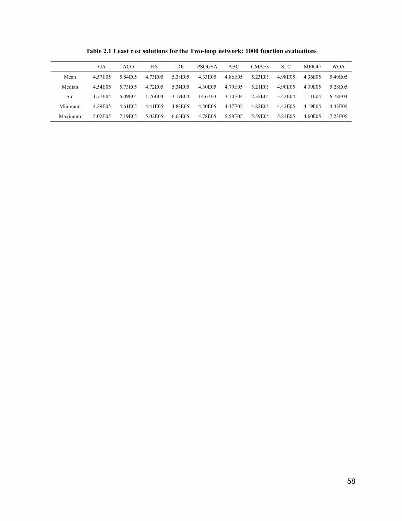
58

Table 2.1 Least cost solutions for the Two-loop network: 1000 function evaluations

GA ACO HS DE PSOGSA ABC CMAES SLC MEIGO WOA

Mean 4.57E05 5.84E05 4.73E05 5.38E05 4.33E05 4.86E05 5.23E05 4.98E05 4.36E05 5.49E05

Median 4.54E05 5.73E05 4.72E05 5.34E05 4.30E05 4.79E05 5.21E05 4.90E05 4.39E05 5.28E05

Std 1.77E04 6.09E04 1.76E04 3.19E04 14.67E3 3.10E04 2.32E04 3.42E04 1.11E04 6.78E04

Minimum 4.29E05 4.61E05 4.41E05 4.82E05 4.20E05 4.37E05 4.82E05 4.42E05 4.19E05 4.43E05

Maximum 5.02E05 7.19E05 5.02E05 6.00E05 4.78E05 5.58E05 5.59E05 5.81E05 4.60E05 7.23E05

59

Table 2.2 Least cost solutions for the Two-loop network: 10000 function evaluations


Mean 4.47E05 4.54E05 4.21E05 4.21E05 4.30E05 4.20E05 4.21E05 4.20E05 4.25E05 5.03E05

Median 4.48.E05 4.55.E05 4.20.E05 4.20.E05 4.29.E05 4.20.E05 4.20.E05 4.20.E05 4.20.E05 4.98.E05

Std 1.77.E04 8.50.E03 3.62.E03 1.11.E03 9.53.E03 4.53.E02 6.98.E03 1.28.E03 8.91.E03 3.91.E04

Minimum 4.20.E05 4.34.E05 4.19.E05 4.19.E05 4.19.E05 4.19.E05 4.19.E05 4.19.E05 4.19.E05 4.43.E05

Maximum 4.95.E05 4.69.E05 4.32.E05 4.22.E05 4.46.E05 4.20.E05 4.27.E05 4.24.E05 4.43.E05 5.81.E05

60

Table 2.3 Least cost solutions for the Two-loop network: 40000 function evaluation


Mean 4.31E05 4.37E05 4.20E05 4.19E05 4.24E05 4.19E05 4.22E05 4.19E05 4.22E05 4.67.E05

Median 4.27E05 4.38E05 4.19E05 4.19E05 4.20E05 4.19E05 4.20E05 4.19E05 4.20E05 4.53.E05

Std 1.06E04 6.13E03 1.90E03 3.48E02 8.81E03 1.87E02 2.29E03 5.10E02 6.93E03 4.85.E04

Minimum 4.20E05 4.23E05 4.19E05 4.19E05 4.19E05 4.19E05 4.19E05 4.19E05 4.19E05 4.22.E05

Maximum 4.51E05 4.46E05 4.27E05 4.20E05 4.45E05 4.20E05 4.43E05 4.20E05 4.43E05 6.48.E05

61

Table 2.4 Least cost solutions for the Hanoi network: 1000 function evaluations


Mean 1.7E07 2.2E08 4.5E07 8.2E07 1.34E07 3.2E08 6.5E07 8.3E06 8.5E06 8.7E06


Std 8.6E06 5.9E07 1.6E07 4.3E07 7.35E06 1.4E08 4.4E07 3.3E06 4.0E05 5.0E05



62



Mean 6.6E06 8.3E06 7.1E06 6.7E06 7.74E06 7.0E06 6.4E06 6.3E06 6.6E06 8.4E06


Std 1.4E05 1.5E06 1.1E05 7.7E04 8.49E05 1.9E05 3.6E04 1.5E05 1.7E05 3.5E05



63



Mean 6.5E06 7.0E06 6.7E06 6.4E06 6.72E06 6.7E06 6.2E06 6.2E06 6.4E06 8.0E06


Standard Deviation

1.8E05 7.8E04 7.8E04 2.8E04 1.65E05 8.6E04 1.3E04 1.4E05 1.2E05 3.8E05



64

Table 2.7 Least cost solutions for the Farhadgerd network: 1,000 function evaluations


Mean 3.0E07 3.5E07 3.2E07 3.5E07 3.03E07 3.5E07 3.1E08 3.2E07 3.2E07 3.5E07


Standard Deviation

1.1E06 9.1E05 1.4E06 9.6E05 2.11E06 1.6E06 6.7E08 1.67E06 4.7E06 3.4E06


Maximum 3.2E07 3.7E07 3.4E07 3.6E07 3.58E07 3.8E07 2.5.E+9 3.43E07 3.6E07 4.1E07

65



Mean 2.3E07 3.1E07 2.4E07 2.3E07 2.65E07 2.5E07 1.9E07 2.09E07 2.3E07 3.5E07


Standard Deviation

1.0E06 8.5E05 4.7E05 4.4E05 1.29E06 1.1E06 2.1E05 5.65E05 7.9E05 2.9E06



66



Mean 2.1E07 2.8E07 2.2E07 2.0E07 2.28E07 2.3E07 1.8E07 1.8E07 2.0E07 3.3E07


Standard Deviation

8.9E05 9.2E05 3.3E05 2.7E05 1.8E06 8.3E05 9.2E04 3.0E05 3.4E05 3.2E06



67

Figure 2.1 Two-loop network

68

Figure 2.2 Hanoi network

69

Figure 2.3 Farhadgerd network

70

a) 1,000‐Function Evaluation

b)10,000‐Function Evaluation

c)40,000‐Function Evaluation

Figure 2.4 Results of Friedman test for: a) 1,000, b) 10,000, and c) 40,000 function evaluations of three networks

71

Chapter 3 : Nondominated Sorting Differential Evolution Algorithms for

Multi-Objective Optimization of Water Distribution Systems

3.1 Preface

Figure 1.1 has listed some population-based EAs for multi-objective design of WDNs such as

NSGA and NSDE. Similar to single-objective design of WDNs in Chapter 2, multi-objective

design of reliable looped WDNs is challenging because these problems comprise nonlinear

relationships between discharge and energy in the pipes and junctions, and nonconvex objective

functions that relate cost and reliability to discrete choices of pipe diameters. The second objective

in these problems is reliability of service, often measured with surrogates such as the resilience

index of Todini (2000). By examining the entire population and evaluating those members that

dominate in terms of two objectives, nondominated sorting algorithms efficiently identify the

Pareto optimal front in multi-objective problems, and one such algorithm, the improved NSGA-II,

has been applied successfully to evaluate the cost-reliability tradeoff for WDNs. The NSDE

algorithm, which takes advantage of the mutation operations in DE and nondominated sorting, and

its variation NSDE-RMO, have been demonstrated as efficient for solving multi-objective

problems. In this chapter, NSDE and NSDE-RMO are applied to discrete WDN optimization for

the first time, and their high performance is demonstrated and compared with NSGA-II and the

AMALGAM method, a widely applied hybrid metaheuristic multi-objective algorithm. For several

networks, NSDE and its variation perform similarly to or better than NSGA-II and AMALGAM.

3.2 Abstract

Optimal design of reliable looped water distribution systems (WDSs) is challenging because these

problems comprise non-linear relationships between discharge and energy in the pipes and

junctions, and non-convex objective functions that relate cost and reliability to discrete choices of

pipe diameters. Efficient algorithms for identifying optimal WDS designs must also be practical

for realistic systems. Differential Evolution (DE) Algorithms, which harness the mutation operator

to identify populations containing very different alternatives, have been shown to be more efficient

than other heuristics for solving single objective versions of these problems, e.g., minimizing the

cost of WDSs. By examining the entire population and evaluating those members that dominate

in terms of two or more objectives, nondominated sorting algorithms efficiently identify the Pareto

optimal front in multi-objective problems, and one such algorithm, the Improved Nondominated

72

Sorting Genetic Algorithm, NSGA-II, has successfully been applied to evaluate the cost-reliability

trade-off for WDSs. The Nondominated Sorting Differential Evolution (NSDE) Algorithm, which

takes advantage of the mutation operations in DE and nondominated sorting, and its variation,

NSDE with ranking-based mutation (NSDE-RMO), have been demonstrated as efficient for

solving multi-objective problems. In this paper we apply NSDE and NSDE-RMO to discrete WDS

optimization for the first time, and demonstrate their high performance compared with NSGA-II

and the multi-algorithm, genetically adaptive multi-objective, AMALGAM method, a widely

applied hybrid meta-heuristic multi-objective algorithm. For three benchmark networks, NSDE

and its variation perform similarly to or better than NSGA-II and AMALGAM except at high cost

levels. For hypothetical randomly generated networks ranging from 100 to 400 nodes, and 100 to

800 pipes, the Pareto optimal front of the NSDE Algorithms dominate all other algorithms,

exhibiting more, and more-varied, Pareto optimal solutions, and converging sooner.

3.3 Introduction

The optimal design of water distribution systems (WDSs) is often considered a least-cost

optimization problem with pipe sizes being the primary discrete decision variables. Early solution

approaches formulate these problems as continuous optimization models and round off the

optimum values of the design variables to the nearest commercial pipe sizes. However, in many

cases, the rounding off of some variables changes the values of others, and the resultant solutions

violate constraints or are suboptimal. Given their efficiency in globally searching the solution

space, evolutionary search methods such as Genetic Algorithms (GAs) (Dandy et al. 1996; Savic

and Walters 1997), Ant Colony Optimization (Maier et al. 2003), Shuffled Frog Leaping (Eusuff

and Lansey 2003), Particle Swarm Optimization (Suribabu and Neelakantan 2006), Harmony

Search (Geem 2006), Dynamically Dimensioned Search Algorithms (Tolson et al. 2009), Honey

Bee Mating Optimization (Mohan and Babu 2010), Differential Evolution (DE) Algorithms

(Suribabu 2010; Zheng et al. 2012; Dong et al. 2012), and Soccer League Competition (Moosavian

and Roodsari 2014), have been applied for solving these and other discrete optimization problems.

The Differential Evolution (DE) Algorithm (Storn and Price 1997), which is similar to, but more

efficient than GA, emphasizes mutation with a mutation operator that sources its genetic

information for trial vectors from three or more random solution vectors, combines trial vectors to

seek better solutions, and thereafter focuses on the most promising solutions. It converges to stable

73

solutions rapidly, is readily adaptable to a wide array of non-linear functions, has been proven to

outperform most other evolutionary search methods for continuous problems (Rozenberg et al.

2005), and is earning the reputation as the first choice in discrete WDS least-cost optimization

(Suribabu 2010; Zheng et al. 2012; Dong et al. 2012).

The reliability of a WDS to provide required water for users under all conditions, including during

pipe bursts or as components deteriorate, is increasingly identified as a key consideration and

competing objective in WDS design. Todini (2000) demonstrates the shortcomings of single-

objective least-cost optimization approaches and explores the application of multi-objective

optimization for minimizing cost and maximizing reliability. He introduces a surrogate for

reliability, the resilience index, and proposes a simple heuristic that emulates the reasoning of an

engineer whose goal is to reduce cost while preserving an acceptable level of reliability of the

system to handle possible failures. While other surrogates for reliability have been examined, e.g.,

modifications of Todini’s index as a function of the diameters of pipes selected (Prasad and Park

2004), maximum head deficiency (Farmani et al. 2005b), flow entropy (Prasad and Tanyimboh

2008), and a combination of these (Raad 2011), Todini’s resilience index is the most widely used,

and in all cases, reliability and cost are competing objectives, requiring multi-objective analysis.

Evaluation of the nondominated set of WDS solutions, the Pareto optimal front, has been achieved

using meta-heuristics such as ranked-based fitness assignment methods for Multi-Objective

Genetic Algorithms, MOGAs (Fonseca and Fleming 1993), Strength Pareto Evolutionary

Algorithms, SPEAs (Zitzler and Thiele 1999), and Nondominated Sorting Genetic Algorithms,

NSGAs (Srinivas and Deb 1994), and more recently with hybrid meta-heuristics such as the multi-

algorithm, genetically adaptive multi-objective, AMALGAM (Vrugt and Robinson 2007) method,

which applies simultaneous multi-method search of the fitness landscape and genetically adaptive

offspring creation. For applications and comparisons of these, see, e.g., Farmani et al. (2005a) and

Raad et al. (2009).

NSGA-II (Deb et al. 2002), an advanced nondominated sorting algorithm, is arguably the most

popular multi-objective evolutionary algorithm, and is increasingly used in WDS design (Farmani

et al. 2006). It features implicit elitist selection based on the Pareto dominance rank, and a

secondary selection method based on crowding distance, which significantly improves the

performance of NSGA on difficult multi-objective problems. Having adopted the mechanisms of

crossover and mutation in its GA, however, NSGA-II faces many of the challenges of GA, such

74

as unstable and slow convergence, and difficulty in escaping from local optima (Storn and Price

1997; Iorio and Li 2004; Peng et al. 2009).

To overcome these limitations, Angira and Babu (2005) substitute the DE Algorithm for the GA

in NSGA-II and develop the Nondominated Sorting Differential Evolution Algorithm (NSDE). A

variation of NSDE, NSDE with ranking-based mutation (NSDE-RMO), uses the ranks of the

population members to modify the mutation operator (Chen et al. 2014). Both NSDE and NSDE-

RMO exhibit improved stability, accelerated convergence, and increased diversity of solutions in

applications to continuous multi-objective problems, and given the high performance of DE in

single objective WDS design, show potential for optimizing WDSs in terms of cost and reliability.

This paper explores this potential with a comparative analysis of these algorithms.

In the following section, we review the two objective functions of cost and reliability, as well as

the hydraulic and design limitations of WDSs, and develop the general WDS design problem. In

Section 3, the NSDE and NSDE-RMO Algorithms are described in the context of WDS design.

Next, the performance of the NSDE Algorithms for designing multi-objective WDSs is compared

with that of NSGA-II and the AMALGAM method in applications to the Two-loop and Hanoi

(Alperovits and Shamir 1977), and the Farhadgerd (Moosavian and Jaefarzadeh 2014) benchmark

networks, and in numerical examples of hypothetical randomly generated networks. Conclusions

are summarized in Section 5.

3.4 Cost and Reliability in Water Distribution Systems (WDSs)

The optimal design of a WDS is defined as the best combination of component sizes and settings,

e.g., pipe size diameters, pump types, pump locations and maximum power, and reservoir storage

volumes, that satisfies the network objectives, such that hydraulic laws of continuity of flow and

energy are maintained, and flow and pressure requirements at the consumer nodes, or other

constraints reflecting network-specific considerations, are met. In this paper, the design of a new

WDS is formulated to optimize cost and reliability objectives with the selection of pipe sizes as

the decision variables, while pipe layout and its connectivity, nodal demands, and minimum head

requirements are imposed. The optimization simultaneously minimizes cost (Eq. 3.1) and

maximizes reliability (Eq. 3.2):

75

𝑀𝑖𝑛 𝐶𝑜𝑠𝑡 𝐶 𝐷 𝐿 (3.1)

𝑀𝑎𝑥 𝐼∑ 𝑞 𝐻 𝐻

∑ 𝑄 𝐻 ∑ 𝑃𝛾 ∑ 𝑞 𝐻

(3.2)

where Li = length of each pipe (meters); Ci (Di) = cost of a pipe of a given diameter ($/meter); Di

= diameter of the selected pipe (meters); np = number of pipes; nn = number of nodes; no = number

of reservoirs; qk = flow demand at node k (meters3/second); Hk = available pressure head at node

k (meters); 𝐻 = minimum pressure head required at all nodes (meters); Qk = supply at a reservoir

located at node k (meters3/second); H0k = elevation head of a reservoir located at node k (meters);

Pi = power of a pump located in pipe i (watts); and γ = specific weight of water (Newtons/ meters3).

Eq. (3.2) is the expression for Todini’s resilience index (Todini 2000) and ranges from 0 to 1,

where a higher value represents a higher reliability. This multi-objective problem is solved subject

to the following constraints:

Continuity at nodes

For each node, continuity should be satisfied,

𝑄 𝑄 𝑞 , ∀ 𝑘 𝜖 𝑛𝑛 (3.3)

where Qin and Qout = flow into and out of node k (meters3/second), respectively.


The total head loss around a closed loop should be equal to zero, or the head loss along a loop

between the two fixed head reservoirs should be equal to the difference in water level of the

reservoirs:

ℎ𝑓

∆𝐻, ∀ 𝑙 𝜖 𝑛𝑙 (3.4)

where hfi = head loss due to friction in the pipe i (meters). We use the Hazen-Williams formula to

define the pressure head loss in each pipe of the network (Williams and Hazen 1914).


For each node, the pressure head should be greater than the prescribed minimum pressure head.

76

𝐻 𝐻 , ∀𝑘𝜖𝑛𝑛 (3.5)


The diameter of the pipes should be available from a commercial size set:

𝐷 𝐷 1 , 𝐷 2 , … , 𝐷 𝑆 , ∀ 𝑖 𝜖 𝑛𝑝 (3.6)

where S = the number of candidate diameters.

3.5 Differential Evolution Algorithms for Multi-Objective Design of WDSs

Optimal WDS design is a combinatorial Non-deterministic Polynomial-hard (NP-hard) problem,

requiring hydraulic simulation to evaluate Eqs. (3.3)-(3.4) for every candidate solution. As the

size of the WDS increases, the combinatorial set of pipe diameter options is on the order of npS,

and the computational burden of the hydraulic simulations increases exponentially. Because they

generate an array of solutions distributed throughout the feasible region at each iteration of the

algorithm, thus reducing the potential for getting trapped at local optima, evolutionary search

algorithms are attractive for addressing NP-hard problems. Among these, DE algorithms obtain a

wider distribution of solutions within the feasible region, and for NP-hard problems have been

shown to accelerate the optimization process. The dominance of DE over other evolutionary and

search algorithms has been demonstrated in the least-cost design of WDS benchmark networks

(Suribabu 2010; Zheng et al. 2012; Dong et al. 2012). DE Algorithms are even more beneficial in

the face of multiple objectives, where evaluation of the Pareto optimal front is enhanced by the

breadth of the arrays of candidate solutions. NSDE has been successfully applied to many

nonlinear and NP-hard multi-objective problems (see, e.g., Angira and Babu 2005; Peng et al.

2009) and a new variation, NSDE-RMO (Chen et al. 2014), which has been applied to continuous

nonlinear optimization test problems, shows promise for discrete cases.

3.5.1 Differential Evolution (DE)

As in GA, the set of decisions, e.g., the candidate design diameters for all pipes in the network, of

the DE Algorithm, are represented as a chromosome, and each decision, or diameter of a given

pipe, is represented as a gene in the chromosome. Candidate diameters are limited to commercially

available pipe sizes and the iterative global search for the best set of chromosomes begins with an

initial population of chromosomes, or combinatorial sets of pipe diameters, NPOP in size, that is

randomly generated over the range of commercially available sizes. At each iteration, or

77

generation, NPOP chromosomes are defined and allowed to reproduce as a function of their

performance, and via crossover of genetic material and mutation. Because both GA and DE are

unconstrained search algorithms, both use penalty functions to track and account for violations of

problem constraints. In DE, a chromosome is designated as a set of real numbers, which are

equivalent to the commercial pipe size selected for the corresponding pipe, and the mutation

operator plays the dominant role in reproduction. At each generation, each chromosome is defined

as Xj, where j = 1, …NPOP. Each Xj experiences mutation, and mutation is achieved by acquiring

genetic material from three or more randomly selected parent solutions in the current generation,

forming a new chromosome 𝑋 . Thereafter, each Xj has the potential to crossover with 𝑋 .

Storn and Price (1997) provide several formulations for 𝑋 , where the formulation most

commonly used in WDS design (see, e.g., Suribabu 2010; Zheng et al. 2012; Dong et al 2012) is:

𝑋 𝑋 𝐹 𝑋 𝑋 (3.7)

where XA, XB, and XC = random solution vectors; and F = mutation scale factor that is designated

to be between 0 and 1.

For a given chromosome, Xj, a gene is designated as Xji, for all i= 1, …np, and correspondingly for

every new chromosome, 𝑋 , the genes are designated 𝑋 , for all i= 1, 2,…np. For every

member of the population, the crossover operation governs whether and where the mutant vector

𝑋 is allowed to breed with Xj, and is defined as follows:

𝑋𝑋

𝑋 𝑖𝑓 𝑟𝑎𝑛𝑑 𝐶𝑅 𝑜𝑟 𝑖 𝑠𝑛, 𝑖 1,2, … 𝑛𝑝

𝑜𝑡ℎ𝑒𝑟𝑤𝑖𝑠𝑒

(3.8)

where rand generates a random value between 0 and 1; CR = crossover rate, designated to be

between 0 and 1; and sn = random integer value between 1 and np that corresponds to a location

in the string of genes. This ensures that the child of Xj inherits at least one decision from 𝑋 .

Finally, selection of the fittest chromosomes in each generation is based on a comparison of the

objective function values of Xj and 𝑋 after mutation and crossover occur.

The three steps of DE, mutation, crossover, and selection, are performed sequentially and are

repeated at every generation throughout the optimization cycle. The algorithm stops when a

stopping criterion is met, e.g., when there is no further improvement of the objective function, or

when the allowable number of function evaluations is reached.

78

3.5.2 Nondominated Sorting Differential Evolution (NSDE)

In NSDE, the accelerated mutation and crossover process of DE is employed, but like NSGA-II,

its goal is to identify the non-inferior set of solutions to a multi-objective problem. Here the

selection process is significantly different than that of DE. Once Xj and 𝑋 are determined, rather

than comparing them with each other in terms of a single objective, they are compared with the

entire 2*NPOP set of solutions for the given generation, in terms of the multiple objectives. Sorting

of the 2*NPOP solutions is undertaken firstly by fast nondominated sorting, i.e., solutions sorted

based on their nondominance rank, and secondly by crowding distance, i.e., solutions within a

non-dominance rank sorted in descending order of their normalized crowding distance. After

sorting is achieved, the top ranked NPOP solutions are then allowed to survive to the next

generation. An advantage of this approach is that, since crowding distance is incorporated in the

sorting procedure, selected solutions are more likely to be distributed along the Pareto optimal

front, see Srinivas and Deb (1994) and Deb et al. (2002) for additional details and discussion of

the advantages of the nondominated sorting procedure.

3.5.3 Nondominated Sorting Differential Evolution with Ranking-based Mutation (NSDE-

RMO)

As in the NSDE approach, NSDE-RMO ranks population members according to their objective

performance and crowding distance, but uses these ranks to modify the mutation operator, as well

as to sort in the selection process. The probability of each chromosome to mutate is defined as

follows:

𝑃𝑟𝑁𝑃𝑂𝑃 𝑅𝑎𝑛𝑘

𝑁𝑃𝑂𝑃

(3.9)

where Prj = probability of selection for the jth population member; and Rankj = rank of the solution

for member j in the population (Chen et al. 2014).

By assigning higher ranked solutions with a higher probability of mutation, NSDE-RMO enhances

the transfer of genetic information that is beneficial for producing high performance solutions and

accelerates convergence to the Pareto optimal front.

79

3.6 Multi-objective Design of WDSs

For each combinatorial set of pipe diameters for the network, i.e., each chromosome, hydraulic

simulation is applied to evaluate Eqs. (3.3)-(3.4) to obtain pressure heads, Hk, for all nodes of the

network. Since Eq. (3.5) must be satisfied, and evolutionary algorithms do not accommodate such

constraints, violations of Eq. (3.5) are tracked, assigned a penalty, and added to the cost objective

function in Eq. (3.1), The penalty is defined as:

𝐶𝑃 𝜆 𝑚𝑖𝑛𝐻

𝐻1, 0

(3.11)

where CPk = penalty associated with node k; and λ = penalty multiplier.

Hk are also used to calculate the reliability, Eq. (3.2). To assure solutions that satisfy Eq. (3.5), the

magnitude of should be sufficiently large. The hydraulic simulation is undertaken with a Global

Gradient Algorithm (GGA) (Todini 2000) implemented in MATLAB.

The performance of the NSDE Algorithms is compared with that of NSGA-II and AMALGAM,

for three benchmark networks, the Two-loop, the Hanoi, and Farhadgerd benchmark networks and

for three hypothetical networks chosen to represent a range of larger WDSs. In most cases, the

minimum pressure limitation is 30 m above ground level, with the exception of the Farhadgerd

network, which must meet the local standard of 20 m. In all cases, the population, NPOP, is 100.

For each of the algorithms, parameter values are selected based on those recommended from the

literature. For NSGA-II, these values are 90% probability of crossover and 3% probability of

mutation based on Farmani et al. (2005a), and for NSDE and NSDE-RMO, 30% probability of

crossover and mutation scale factor of 0.5 (Chen et al. 2014). AMALGAM self-adapts, given a

range for each parameter value, and these are provided in Vrugt (2015). Calibration of the

parameters for multi-objective network problems is not trivial and is beyond the scope of this

paper. For a discussion of calibration of evolutionary algorithms for single objective network

problems, see Marchi et al. (2014).

3.7 Benchmark and Experimental Networks

The Two-loop network has seven nodes, eight pipes, and two loops, and is fed by gravity from a

reservoir with a 210-m fixed head. The pipes are all 1,000 m long with a Hazen-Williams

coefficient of 130, and there are 14 candidate commercial pipe diameters available. Although the

80

Two-loop network is small, a complete enumeration comprises 148= 1.48 ×109 different network

designs, thus making this illustrative example difficult to solve. The Hanoi network is a more

complex compilation of loops and branches, has 32 nodes, 34 pipes and three loops, and is fed by

gravity from a reservoir with a 100-m fixed head. The pipe lengths vary from 100 to 3500 m, with

a Hazen-Williams coefficient of 130, and six candidate commercial pipe diameters. The

Farhadgerd, Iran, network is a detailed representation of the water mains for a community of 8200

people. It has 68 pipes, 53 nodes, and 12 loops, and is fed by gravity from a reservoir with a 510-

m fixed head. The pipe lengths vary from 5 to 885 m, with a Hazen-Williams coefficient of 130,

and nine candidate commercial pipe diameters. For detailed hydraulic and cost information for

these benchmark networks see Alperovits and Shamir (1977) and Moosavian and Jaefarzadeh

(2014), for the Two-loop and Hanoi, and Farhadgerd benchmark networks, respectively.

Three additional hypothetical networks are randomly generated to expand the range of network

sizes. In all cases, for the specified numbers of nodes and pipes, whether a pipe connects any two

nodes is randomly determined with equal likelihood, and the network is formed under the condition

that each pipe connects only two nodes, and each node is connected to at least two pipes. For

every 20 nodes, a source reservoir with a constant fixed pressure head is randomly assigned to one

of the nodes, and all other nodes of the network are assumed to be at sea level (see, e.g., Zecchin

et al. 2012). The parameters of each reservoir and pipe are independently sampled from uniform

distributions as follows: reservoir elevation = u [50, 100], nodal demands = u [0, 0.1], and pipe

length = u [500, 650], where u [LB, UB] symbolizes a random variable uniformly distributed

between LB and UB. The Hazen-Williams coefficient of all pipes is assigned a constant value of

130 and as for the benchmark networks, the direction of flow is determined with the hydraulic

simulator. For these networks, 20 candidate commercial pipe diameters are possible, ranging from

50 to 1000 mm, in increments of 50 mm. The smallest of these networks has 100 nodes and 200

pipes and the largest network has 400 nodes and 800 pipes. The number of combinatorial sets of

pipe diameter options for these networks range from 20200 to 20800, complicating the identification

of the multi-dimensional fitness landscape, and increasing the difficulty in identifying Pareto

optimal decisions. For all networks, the value of λ, the penalty weight in Eq. (3.11), is selected to

be the maximum cost for the given network, i.e., the sum of the costs, assuming that for all pipes,

the maximum diameter is chosen.

81

3.8 Performance of Multi-objective Optimization Algorithms

In order to evaluate the number of required generations to approximate the Pareto optimal front,

for each benchmark and hypothetical network, all nondominated sorting algorithms are executed

20 times. Each algorithm is stopped when there is no further change in the cost-reliability Pareto

optimal front, expressed by the minimum, median and maximum solutions, for 50 generations.

Table 3.1 provides the average values of the costs, resilience indices, and generations for the 20

algorithm executions. In all cases, the pressure constraints, see, e.g., Eq. (3.5), are satisfied, and

thus there are no infeasible solutions. Being a black-box, hybrid meta-heuristic, the AMALGAM

method uses the number of generations as the stopping criteria, to be pre-specified by the user.

Thus our IGD-based stopping criteria could not be applied for this method. For the benchmark

networks, the single objective least-cost solutions identified in previous studies are also provided

in the table. For all executions of the algorithms, the minimum cost calculated for the multi-

objective WDS design is greater than the single objective least-cost solution. This shows that no

algorithm is able to explore the entire Pareto front using the specified algorithm parameters.

However, as shown in Table 3.1, NSDE and NSDE-RMO have explored this part of the Pareto

front better than NSGA-II and, with the exception of the Hanoi case study, found cheaper solutions.

As one measure of the accuracy of the approximated set of nondominated solutions, or the speed

of convergence of an algorithm to a near optimal solution, the Inverted Generational Distance

(IGD) determines the average distance of the uniformly distributed Pareto optimal solutions

obtained after a very large number of generations to the approximated nondominated surface.

Small values of IGD are preferred and the rate at which small values are achieved indicates the

rate of convergence. For a detailed development of the IGD measure and a discussion of its

shortcomings see Zitzler et al. (2003) and Maier et al. (2014).

Based on the findings in Table 3.1, 20 additional algorithm executions were undertaken, for 500,

1000, and 2000 generations, for the Two-loop, Hanoi and Farhadgerd, and hypothetical networks,

respectively. Figures 3.1-3.3 show one Pareto optimal front for the benchmark networks. Figures

3.4-3.6 are similar figures for the hypothetical networks. These are the Pareto optimal fronts with

the lowest final IGD, among the 20 executions of the algorithms. For the Two-loop network, the

cost-reliability trade-off is nearly the same for all algorithms, where the cost ranges from $420,000

82

to $4.4 million for all four algorithms, and the resilience index from 0.029 to 0.113, for the NSDE

Algorithm, and approximately 0.043 to 0.113 for all other algorithms.

For the Hanoi network, the performance of the nondominated sorting algorithms is also similar,

although they are unable to find solutions at the extreme upper range of the frontier. Here the

performance of NSGA-II and AMALGAM are high, though AMALGAM generates more of the

upper range of the frontier and NSGA-II generates more of the lower range. This reinforces similar

findings in Wang et al (2014), where, for the Hanoi network, NSGA-II shows better convergence

than AMALGAM for the majority of the Pareto optimal front, but only AMALGAM generates

solutions at high reliability levels. As Vrugt and Robinson (2007) note, the Strength Pareto sorting

approach in AMALGAM ensures that unique individuals survive to the next generation, thus

enhancing its performance at the extreme ends of the frontier, and this characteristic is

demonstrated for this network.

For the Farhadgerd network, NSGA-II generates a narrow portion of Pareto optimal front, with

costs ranging from $1.87 to $4.65 million and resilience index from 0.56 to 0.66. Here

AMALGAM generates solutions at the upper range of the frontier, and NSDE and NSDE-RMO

generates those at the lower range of the frontier. The mutation operator in the NSDE Algorithms

enhances their ability to rapidly identify points on the Pareto optimal front, and the ranked-based

sorting mutation operator in NSDE-RMO enhances its ability to expand the frontier as more

generations pass.

As shown in Figures 3.4-3.6, the performance of nondominated sorting algorithms is comparable

for the smallest hypothetical network, with NSDE and NSDE-RMO identifying a wider range of

non-inferior points. In general, as the network size increases, the NSDE-RMO solutions dominate

those of all other algorithms, and the NSDE Algorithm performs well, though not as well as the

NSDE-RMO. The performance of the NSGA-II Algorithm and AMALGAM method drops

significantly as the network size increases.

The results for the WDS with 400 nodes and 800 pipes, WDS400x800, indicate that, while the

NSDE and NSDE-RMO Algorithms appear to be trending toward dominance, the solutions have

not converged to the Pareto Optimal Front for any of the algorithms, suggesting that the population

number or the number of generations is insufficient for all algorithms. However, NSDE-RMO

83

does provide the solution with the minimum cost ($116 million) and the highest reliability with a

resilience index of 0.615.

Figures 3.7-3.12 provide the IGD values for the benchmark and hypothetical networks, where the

final Pareto optimal fronts in Figures 3.1-3.6 are considered as the reference ideal trade-off. For

the Two-loop and Hanoi networks, the ALMALGAM method converges faster than other

algorithms, but in general, as the network size increases its convergence slows relative to that of

all other algorithms. With the exception of WDS400X800, which has not yet converged, the

performance of NSDE and NSDE-RMO are similar for most network sizes, and are greater than

for other algorithms, though NSDE-RMO performs slightly better overall.

3.9 Conclusion

NSDE and NSDE-RMO are efficient for evaluating trade-offs between cost and reliability in WDS

design. Moreover, they are particularly effective for evaluating solutions in the highest cost-

benefit portion of the solution space (i.e., high-resilience, low-cost solutions), which may be of

high interest to practitioners. Discrete large NP-hard problems like WDS design require the

consideration of many different solutions and the mutation advantage of DE is particularly

effective at generating diverse sets of solutions. The mutation operator of DE, compared with that

of GA and other evolutionary algorithms, provides candidate solutions with very different

characteristics. This feature enhances its ability to escape local optima and, combined with the

selection function of nondominated sorting, is the main reason that NSDE is attractive for

analyzing multi-objective discrete large problems.

In a comparison analysis of benchmark and hypothetical networks, NSDE and NSDE-RMO

generally perform as well or better than NSGA-II and AMALGAM except for the Hanoi and

Farhadgerd networks where, at the extreme end of the Pareto optimal front, AMALGAM performs

well. NSDE-RMO is typically more effective than NSDE. Its ability to rapidly identify the Pareto

optimal front, due to its ranked-based selection mechanism, makes it an attractive algorithm

overall.

The WDS analysis results show promise for the use of NSDE and NSDE-RMO in the multi-

objective analysis of large and more realistic networks. The use of these algorithms may provide

opportunities for expanding the objectives to be considered in WDS design, and for including

additional definitions of reliability in the objective set.

84

The high performance of the NSDE Algorithms is further evidence of the advantages of

nondominated sorting, and of the clear potential of ranked-based sorting, in multi-objective

evolutionary optimization. Advances in multi-objective optimization and WDS design may be

directed at harnessing this potential, for example, by modifying AMALGAM to include ranked-

based sorting as part of its sorting procedure. Moreover, the efficiency of NSDE may be further

improved by incorporating other sorting procedures, such as the Strength Pareto sorting approach,

which shows potential for defining the extreme end of the Pareto frontier.

85

Table 3.1 Average of twenty executions of the algorithms

Network Type (diameter options)

Least cost

Average

Min Cost($)

Average Median Cost ($)

Average Max

Cost($)

Average Min

Resilience Index

Average Median

Resilience Index

Average Max

Resilience Index

Average Stopping Generation

Two-Loop Benchmark (14)

NSGA-II 4.54E+05 1.21E+06 4.28E+06 4.99E-02 1.05E-01 1.12E-01 224

$4.19E+51 NSDE 4.29E+05 1.12E+06 4.27E+06 4.24E-02 1.03E-01 1.12E-01 216

NSDE-RMO 4.28E+05 1.11E+06 4.29E+06 4.33E-02 1.03E-01 1.12E-01 179

Hanoi Benchmark (6)

NSGA-II 6.38E+06 7.37E+06 9.77E+06 2.51E-01 3.25E-01 3.53E-01 520

$6.08E+62 NSDE 6.45E+06 7.27E+06 9.08E+06 2.60E-01 3.22E-01 3.48E-01 405

NSDE-RMO 6.42E+06 7.25E+06 9.14E+06 2.54E-01 3.21E-01 3.48E-01 371

Farhadgerd Benchmark (9)

NSGA-II 1.94E+07 2.48E+07 4.29E+07 5.60E-01 6.47E-01 6.56E-01 835

$1.78E+7 NSDE 1.91E+07 2.59E+07 4.35E+07 4.93E-01 6.49E-01 6.56E-01 503

NSDE-RMO 1.90E+07 2.56E+07 4.44E+07 4.95E-01 6.49E-01 6.56E-01 582

WDS100x200 NSGA-II 2.34E+07 3.02E+07 3.93E+07 8.39E-01 8.77E-01 8.78E-01 617

hypothetical network (20)

NSDE 1.95E+07 2.80E+07 5.04E+07 8.24E-01 8.77E-01 8.78E-01 1018

NSDE-RMO 2.00E+07 2.68E+07 4.17E+07 8.06E-01 8.75E-01 8.78E-01 726



NSDE 5.54E+07 6.57E+07 8.55E+07 5.89E-01 6.24E-01 6.32E-01 1145

NSDE-RMO 5.24E+07 6.29E+07 9.01E+07 5.65E-01 6.22E-01 6.32E-01 1503



NSDE 1.30E+08 1.44E+08 1.70E+08 5.87E-01 6.07E-01 6.14E-01 1287

NSDE-RMO 1.16E+08 1.30E+08 1.57E+08 5.73E-01 6.07E-01 6.14E-01 1697

1 From Geem (2006)

2 From Geem (2006) 3 From Lence et al. (2017)

86

Figure 3.1 Pareto optimal front of Two-loop network

0 0.5 1 1.5 2 2.5 3 3.5 4 4.5

x 106

0.02

0.03

0.04

0.05

0.06

0.07

0.08

0.09

0.1

0.11

0.12

Cost

Res

ilien

ce I

ndex

Two-Loop

NSGA-II

NSDE-RMONSDE

AMALGAM

87

Figure 3.2 Pareto optimal front of Hanoi network

6 6.5 7 7.5 8 8.5 9 9.5 10 10.5 11

x 106

0.22

0.24

0.26

0.28

0.3

0.32

0.34

0.36

Cost

Res

ilien

ce I

ndex

NSGA-II

NSDE-RMONSDE

AMALGAM

88

Figure 3.3 Pareto optimal front of Farhadgerd network

1.5 2 2.5 3 3.5 4 4.5 5 5.5 6 6.5

Cost 107

0.35

0.4

0.45

0.5

0.55

0.6

0.65

0.7

Res

ilien

ce In

dex

NSGA-IINSDEAMALGAMNSDE-RMO

89

Figure 3.4 Pareto optimal front for WDN 100x200, 100 nodes and 200 pipes

1.5 2 2.5 3 3.5 4 4.5 5 5.5 6

x 107

0.8

0.81

0.82

0.83

0.84

0.85

0.86

0.87

0.88

Cost

Res

ilien

ce I

ndex

WDS100x200

NSGA-II

NSDE-RMONSDE

AMALGAM

90


4 5 6 7 8 9 10

x 107

0.57

0.58

0.59

0.6

0.61

0.62

0.63

Cost

Res

ilien

ce I

ndex

WDS200x400

NSGA-II

NSDE-RMONSDE

AMALGAM

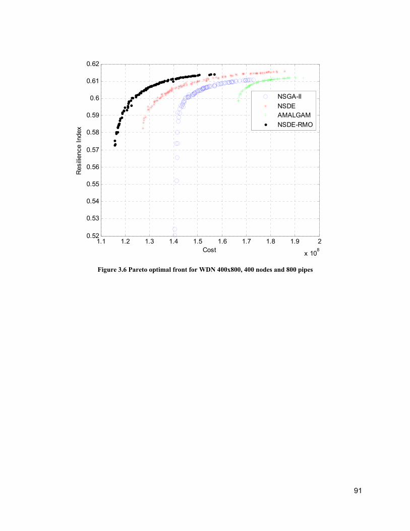
91


1.1 1.2 1.3 1.4 1.5 1.6 1.7 1.8 1.9 2

x 108

0.52

0.53

0.54

0.55

0.56

0.57

0.58

0.59

0.6

0.61

0.62

Cost

Res

ilien

ce I

ndex

WDS400x800

NSGA-II

NSDEAMALGAM

NSDE-RMO

92

Figure 3.7 IGD at each generation for Two-loop network

0 50 100 150 200 250 300 350 400 450 50010

3

104

105

106

Generation

IGD

Two-Loop

NSGA-II

NSDENSDE-RMO

AMALGAM

93

Figure 3.8 IGD at each generation for Hanoi network

0 100 200 300 400 500 600 700 800 900 100010

3

104

105

106

107

108

109

Generation

IGD

NSGA-II

NSDE

NSDE-RMO

AMALGAM

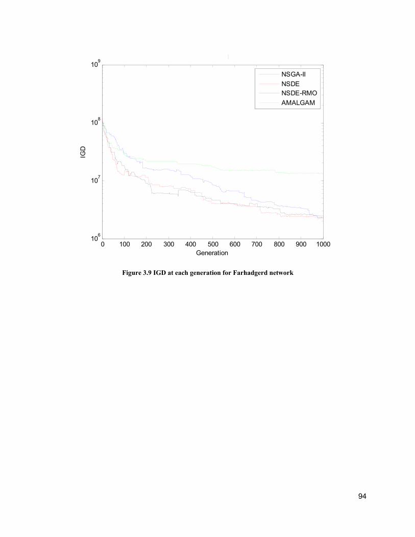
94

Figure 3.9 IGD at each generation for Farhadgerd network

0 100 200 300 400 500 600 700 800 900 100010

6

107

108

109

Generation

IGD

Farhadgerd

NSGA-II

NSDENSDE-RMO

AMALGAM

95

Figure 3.10 IGD at each generation for WDN100x200

0 200 400 600 800 1000 1200 1400 1600 1800 200010

4

105

106

107

108

Generation

IGD

WDS100x200

NSGA-II

NSDENSDE-RMO

AMALGAM

96


0 200 400 600 800 1000 1200 1400 1600 1800 200010

5

106

107

108

Generation

IGD

WDS200x400

NSGA-II

NSDENSDE-RMO

AMALGAM

97


0 200 400 600 800 1000 1200 1400 1600 1800 200010

5

106

107

108

109

Generation

IGD

NSGA-II

NSDE

NSDE-RMO

AMALGAM

98

99

Chapter 4 : Fittest Individual Referenced Differential Evolution Algorithm for

Optimization of Water Distribution Networks

4.1 Preface

In Chapter 2, ten popular EAs are tested and compared for single-objective design of three

networks. While these heuristic algorithms show success in addressing specific WDN design

problems, there is no guarantee that the global optimum may be found or that any one method will

be efficient. Wolpert and Macready (1997) cite the No-Free-Lunch (NFL) theorem, assert that no

one optimization algorithm may be suited for solving all kinds of optimization problems, and

underscore the need for new algorithms that may improve on efforts to reach global optima.

Furthermore, results and analysis of EAs in Chapter 2 show that some characteristics and

properties of the CMAES, SLC, ABC and DE have significant impact on the convergence

properties of these algorithms. Among all other algorithms, DE has the simplest framework and

computing code structure which makes it efficient for solving a wide range of optimization

problems. In this chapter, by maintaining the simple framework of DE and adding some worthy

characteristics of SLC and ABC, a new efficient algorithm, called the Fittest Individual Referenced

Differential Evolution (FDE), is proposed which significantly increases the speed of convergence

in the optimization of WDN design. The fundamental concept of FDE is similar to DE, however,

a counter for each solution vector is defined and used to locate local optimum traps and restart the

algorithm, thus avoiding stagnation positions. This capability is beneficial in network design,

because the problem has various local optima which are sometimes far from eachother and make

finding global optima difficult. Results of optimization for three benchmark networks, the Two-

loop, Hanoi, and NewYork WDN, show that the number of function evaluation under FDE

required to reach the global optimum is fewer than DE. For example for Two-loop network, the

minimum number of function evaluations to find first occurrence of the best solution for FDE is

197 while for DE is 1,320.

4.2 Abstract

Water distribution networks (WDNs) are one of the most essential components in the urban

infrastructure system and require large investment for construction. Design of such networks is

classified as a large combinatorial discrete nonlinear non-deterministic polynomial-hard (NP-hard)

optimization problem. The main concerns associated with optimization of WDNs are related to the

100

nonlinearity of the discharge-head loss relationships for pipes and the discrete nature of pipe

sizes. This paper proposes a new evolutionary algorithm, called Fittest Individual Referenced

Differential Evolution (FDE), which is significantly more efficient and reliable than other

algorithms for optimization of WDN DESIGN problems. The fundamental structure of FDE is

similar to conventional Differential Evolution (DE), though the functions of the mutation and

crossover operators are to exploit good solutions, and explore very different solutions,

respectively, and counting and re-starting mechanisms are introduced to identify local optima and

avoid stagnation. These features are beneficial in WDN design because such problems may have

an array of local optima, which are, at times, far from one another, making finding the global

optima difficult. The mutation and crossover operators are developed to accelerate convergence

and, while the optimal mutation and crossover parameters may vary among networks, the

efficiency of the algorithm reduces the need for adaptive parameters or population size. A

sensitivity analysis is conducted for algorithm parameters and counting and re-starting limits,

based on eight evolutionary algorithm (EA) benchmark test problems, and the efficiency of the

FDE for solving two- and ten-dimensional versions of these problems is demonstrated, using the

most effective values of the parameters and limits. FDE-based optimal designs of three benchmark

WDNs, the Two-loop, Hanoi, and New York Networks, show that a minimum number of function

evaluations (or hydraulic simulations) are required to reach the global optimal, less than 300 in all

cases, compared with the more than 1300 function evaluations required for DE. Furthermore, an

application of FDE to a large-sized network, that for the City of Farhadgerd, Iran, shows that FDE

is significantly more effective than other EAs in terms of its speed of convergence and reliability.

Key words: Evolutionary algorithms, differential evolution algorithm, water distribution networks,

optimization.

4.3 Introduction

Approaches for determining optimal design of water distribution networks (WDNs) and their

appurtenances have been developed based on linear programming, LP (Schaake and Lai (1969);

Alperovitz and Shamir (1977); Quindry et al. (1982); Kessler and Shamir (1989)), and nonlinear

programming, NLP (Lansey and Mays (1989); Duan et al. (1990)) formulations that maximize

design objectives while satisfying the hydraulic rules that govern such systems, and consumer

demands for water quantity, quality and pressure. In an illustration based on the Two-loop

101

benchmark WDN, Bhave and Sonak (1992) demonstrate that LP is less efficient in terms of

computational effort, compared with a heuristic method which initially identifies good branching

configurations for obtaining the global optimum. Cunha and Sousa (1999) posit that NLP

approaches are sophisticated in terms of their use of the fundamental hydraulic equations to recast

the form of the optimization problem and to yield gradient and Hessian information, however, their

inability to restrict the search space to discrete pipe sizes is a significant practical limitation.

In order to identify designs for large networks, and more readily accommodate the discrete and

nonlinear nature of the problem, this paper presents a new evolutionary optimization algorithm

(EA), the Fittest Individual Referenced Differential Evolution (FDE) Algorithm, which

significantly increases the efficiency and consistency of the conventional Differential Evolution

(DE) Algorithm (Storn and Price 1997). DE, like other EAs, is becoming increasingly more

popular for optimization of WDNs and in practical applications, because it: (i) is based on simple

concepts and is easy to implement; (ii) can identify and avoid local optima; and (iii) does not

require a continuous or continuously differentiable objective function. It employs operators,

similar to mutation, crossover (or mating), and selection, to explore the fitness surface, or range of

solutions, and exploit attractive solutions, i.e., mutation seeks to assess all possible good solutions,

and crossover seeks to concentrate these solutions. Because they generate an array of distributed

solutions at each iteration of the algorithm, thus reducing the potential for getting trapped at local

optima, EAs are attractive for addressing NP-hard problems. Among these, DE algorithms have

been shown to obtain a wider distribution of solutions within the feasible region, and accelerate

the optimization process (Storn and Price 1997; Noman and Iba, 2005; Yang et al., 2007).

Many EAs are successfully used to identify WDN designs, see, e.g., applications of Genetic

Algorithms, GAs (Brooke et al. 1988; Lansey and Mays 1989; Duan et al. 1990); Simulated

Annealing, SA (Cunha and Sousa 1999); Harmony Search, HS (Geem 2006); Shuffled Frog

Leaping (Eusuff and Lansey 2003); Ant Colony Optimization, ACO (Maier et al. 2003); Max-min

Ant System (Zecchin et al. 2006); Particle Swarm Optimization, PSO (Suribabu and Neelakantan

2006a and Suribabu and Neelakantan 2006b); Cross Entropy (Perelman and Ostfeld 2007); Scatter

Search (Lin et al. 2007); DE (Vasan and Simonovic 2010); Self-adaptive Differential Evolution,

SaDE (Zheng et al. 2013); Soccer League Competition, SLC (Moosavian and Roodsari 2014); and

Improved Genetic Algorithms (Bi et al. 2015). Recently, combinations of classical optimization

methods and EAs are suggested for WDN design, e.g., Cisty (2010) applies a combination of a

102

simple GA and LP; Haghighi et al. (2011) apply a combination of GA and integer linear

programming (ILP); Zheng et al. (2011) apply a combination of NLP and DE; and Zheng et al.

(2014) apply a combination of binary linear programming (BLP) and DE. All of these algorithm

combinations eventually converge to an appropriate design, although their computational costs are

often significantly greater than those of the aforementioned stand-alone EAs. To accelerate

convergence, hybrid algorithms are developed to improve the efficiency of the search process,

including: Keedwell and Khu (2005) who use a hybrid method in which a cellular automata

approach provides a good initial population for a GA; Tolson et al. (2009) who propose a hybrid

approach which combines two local search heuristics with a discrete search strategy adapted from

a continuous dynamically dimensioned search algorithm; Sedki and Ouazar (2012) who apply a

combination of DE and PSO algorithms; Babu and Vijayalakshmiz (2013) who apply a

combination of PSO and GA; Geem (2013) who applies a combination of PSO and HS algorithms;

Sheikholeslami et al. (2016) who apply a combination of Cuckoo search and HS algorithms; and

Reca et al. (2017) who apply a combination of a search space reduction algorithm and GA.

The dominance of DE over other algorithms has been demonstrated in the least-cost design of

WDS benchmark networks (Suribabu 2010; Zheng et al. 2011; Dong et al. 2012). DE Algorithms

are also beneficial in the face of multiple objectives, where evaluation of the Pareto optimal front

is enhanced by the breadth of the arrays of candidate solutions. Nondominated Search Differential

Evolution (NSDE) has been successfully applied to many nonlinear and NP-hard multi-objective

problems (see, e.g., Angira and Babu 2005; Peng et al. 2009) and a new variation, Nondominated

Search Differential Evolution with Ranking-based Mutation Operators, NSDE-RMO (Chen et al.

2014), which has been applied to continuous nonlinear optimization test problems and multi-

objective WDN design (Moosavian and Lence 2016), shows promise for discrete cases.

Given the efficiency of unaided DE, or DE in combination with other algorithms, for solving an

array of discrete and continuous optimization problems, improvements in the algorithm abound.

These can be classified into: (i) tuning the control parameters, i.e. tuning the mutation and

crossover parameters, (Zheng et al. 2014; Gamperle et al. 2002; Omran et al. 2005; Brest et al.

2006; Das et al. 2005) or population size (Teo 2006); (ii) advancing the selection operator, such

as by introducing ranking-based selection (Gong and Cai 2013; Chen et al. 2014) and statistically-

based selection (Mininno et al. 2011); and (iii) adding new schemes for advancing the operators,

such as by introducing enhanced mutation formulae (Zhao and Liu 2014; Kumar 2017; Cail et al.

103

2017; Maucec et al. 2018), employing a neighborhood search (Yang et al. 2007; Das et al. 2009),

and improving the crossover process (Liang et al. 2014), and (see, e.g., Das et al. (2009) for an in-

depth review of these and other advances in DE). In one example of the latter, the Fittest Individual

Refinement, FIR-modified DE (Noman and Iba 2005), the crossover operator compares each

mutated individual with the individual with the highest fitness, and uses the Simplex Crossover

approach for multiparent recombination of individuals. Thus, in FIR, crossover allows for both

accelerated exploitation of the current best solution, along with exploration of the range of

solutions.

This paper develops and analyzes applications of an improved DE, FDE, which modifies mutation

and crossover operators to accelerate convergence, and employs a counting mechanism to find

local optima traps. Each individual member of the population of solutions undergoes mutation

with the current best solution, and crossover with other randomly selected members of the

population. Thus, in contrast to conventional DE, the mutation operator encourages exploitation

of good solutions, and the crossover encourages exploration of the range of solutions. Local

optima are identified by counting the number of generations in which a given individual solution

survives and, upon reaching a counting limit, eliminating this individual solution from the

population, thereby shrinking the population size. As further local optima are identified, the

population size reduces further, and this process continues until a re-starting limit on the minimum

population size is reached. Thereafter, the algorithm restarts the entire optimization search,

continuing to explore the range of solutions. The FDE Algorithm is efficient for optimization of

WDNs, because this problem has many local optimum solutions, while other EAs cannot always

escape from these locations (Liong and Atiquzzaman 2004; Reca and Martinez 2006; Zecchin et

al. 2006). The performance of FDE is demonstrated for eight EA benchmark test problems, for

three benchmarks WDNs, the Two-loop, Hanoi, and New York networks, and for the WDN for

the City of Farhadgerd, Iran. The results of the application of FDE to eight EA benchmark test

problems are compared with those of DE, and the results of the application of FDE to the

benchmark networks are compared with results from a large array of EA applications reported in

the literature for these problems. For the Farhadgerd WDN, FDE and nine popular EA Algorithms

and metaheuristics are implemented in this work, and all ten of these algorithms are compared in

terms of their efficiency, i.e., the rate at which the global optimum is found, and reliability, i.e., its

consistency in finding the global optimum. The algorithms assessed for the Farhadgerd WDN are

104

GA, SA, HS, DE, PSO, ABC, SLC, the covariance matrix adaptation evolution strategy (CMAES)

(Hansen and Kern 2004), and biology and bioinformatics global optimization (MEIGO) (Egea et

al., 2010; Egea et al., 2014). Results show that the proposed FDE is superior in terms of the number

function evaluations required to reach the global optimum, and consistently does so, over a large

number of applications of the algorithm.

In the following sections, the DE and the proposed FDE algorithms are presented in detail. Next,

a sensitivity analysis regarding the parameters and limits employed in FDE, and a comparison of

the perfomance of DE and FDE, is conducted for eight benchmark test problems for EAs.

Thereafter, the general optimization model formulation for least-cost design of WDNs is briefly

described. Application of FDE to three benchmark and the Farhadgerd WDNs is then

demonstrated and performance of FDE for these networks is assessed, compared with that for an

array of EAs reported in the literature, and nine efficient EAs or metaheuristics, respectively.

Finally, a discussion of the advantages of FDE, and recommendations for future research are

provided.

4.4 Differential Evolution (DE) and Fittest Individual Referenced Differential Evolution

(FDE) Algorithms

Table 4.1 outlines the different steps of the DE and FDE optimization algorithms and describes

their evolution strategies in detail. In both algorithms, and similarly for all EAs, Step 1 is the

initialization of the parameters, i.e.: the mutation, F, and crossover, CR, rates; the coding of the

strings that define the possible decision variable values, for the vectors of decisions that represent

the members of a population; and the number of individuals that comprise the population (NPOP).

In addition to this information, FDE also assigns a counter limit, Counterlimit, and a re-start limit,

Re-startlimit.

Step 2 is the generation of the initial population of decision variable values, for vectors of

decisions, or individual members of the population, and calculation of the corresponding objective

function values for, or the fitness value of, these vectors, i.e., , the generation of random vectors

of decision variable values for an array of solutions, Xj, where j = 1,…, NPOP, that represent the

first generation of a population. In this step, DE assigns a solution vector and the corresponding

objective value for each population member. In addition to these vectors, FDE also assigns a new

variable, called the counter, Counterj, and sets its value to zero.

105

In Step 3, both algorithms conduct two different mutation operations. In DE, the mutation operator

selects three random solution vectors for exploration purposes, XA, XB, and XC. In so doing, it

provides a random search direction for each member of the population. In FDE, XA, XB, and XC are

identified, but the mutation operator is based on a random movement by selection of two random

solution vectors, XA, and XB, around the member of the current population with the highest fitness,

or best objective function value, Xbest, and thus provides dissimilar random search directions for

the best solution thus far. The mutation operation in FDE is designed for exploitation purposes and

by improving the best solution vector at each stage, it accelerates the convergence rate of the

algorithm. Figure 4.1 shows a conceptualization of the different nature of the mutation operators

in DE and FDE.

In Step 4, both algorithms conduct crossover operations. In DE, the crossover operation is

conducted for each Xj, to exploit the search direction which is created through mutation. FDE

introduces a shuffled crossover operator to explore the range of solutions, the fitness landscape,

by randomly moving the modified best solution vector created through mutation. The FDE

crossover operator conducts its process with the random solution vector, XC, instead of 𝑋 . The

shuffling process provides more extensive exploration of the search space in different directions,

thereby reducing the chance of the search getting trapped in local optima. Therefore, by application

of both the mutation and crossover mechanisms, new positions of the population members for both

algorithms may be widely distributed.

In Step 5, both algorithms update the population based on the new solution vector created by the

mutation and crossover operators. In this step, the objective function value corresponding to the

new solution vector is evaluated, and this value is compared with the current solution vector, 𝑋 .

If the objective value of the new solution vector is better than that of 𝑋 , then it enters the

population in place of 𝑋 . Otherwise, 𝑋 remains in the population. A similar comparison is

conducted with the best solution vector (𝑋 ) to update this member after each stage.

In this step, FDE also updates the counter value of the selected member, 𝐶𝑜𝑢𝑛𝑡𝑒𝑟 , i.e., if the new

solution vector is better than that of 𝑋 , the counter is kept at its current value, i.e., zero in the first

generation, otherwise the corresponding counter is increased by one unit, 𝐶𝑜𝑢𝑛𝑡𝑒𝑟 𝐶𝑜𝑢𝑛𝑡𝑒𝑟

1. To show the difference in performance of mutation and crossover operators in the DE and FDE

Aalgorithms, a two-dimensional Sphere Function EA benchmark test problem is employed and the

106

first two iterations of both algorithms are executed. The EA benchmark test problem is

minimization of 𝑓 𝑥, 𝑦 𝑥 𝑦 , with the global optimum solution of 0,0 . Assume that the

initial population for both algorithms is randomly generated as in Table 4.2.

The distribution of the initial population in the X-Y plane is shown in Figure 4.2. The first iteration

of both algorithms, including mutation, crossover and selection, are shown in Table 4.3. After the

first iteration, the best solution obtained by DE is its new point D (2,1) with an objective function

value equal to 5, and an average objective function value for all five points of 14. The best solution

vector for FDE is its new point B (-1, 0.5) with an objective function value equal to 1.25, and an

average objective function value for all five points of 13.15. Furthermore, the number of function

evaluations required for DE to obtain point D is five, and is already 25% higher than that required

for FDE to reach point B, which is 4. Therefore, FDE has slightly better performance even in the

first iteration and can accelerate the convergence process with a lower computational burden.

A similar progression may be observed in the second iteration, as reported in Table 4.4. For the

DE-based solution, the average value of the objective function for all points remains at 14 requiring

ten function evaluations, while for the FDE-based solution, the average value of the objective

function is reduced to 8.86 requiring eight function evaluations.

In Step 6, the DE algorithm checks the termination criteria, e.g., some maximum number of

generations or function evaluations, or some lower limit on the change in global optimum fitness

value, and if the criteria are not satisfied, Steps 3-5 are repeated. The FDE algorithm first checks

the counter value, 𝐶𝑜𝑢𝑛𝑡𝑒𝑟 , of all j = 1, NPOP population members. The counter value of each

member shows how many times this member could not be improved during the evolution process.

If the counter value of a member is greater than the maximum counter value, Counterlimit, it

indicates that stagnation at a local optima has occurred, and that the mutation and crossover

operators alone cannot escape from this local optimum position. Therefore, more evolutions would

not lead to improvement in this vicinity and will simply increase the computational burden

ungainly. In this case, the algorithm eliminates this unprofitable solution from the population and

shrinks the population size accordingly. Reducing the size of the population, reduces the number

of function evaluations in subsequent generations, yet provides for the opportunity for other

members to evolve and progress.

107

If the shrinking process reduces the population size to less than the Re-startlimit, the remainder of

the population is likely to experience difficulty in escaping from the current local or global optima.

Thus, there may be no benefit in further evolving this small-sized population. In this case, FDE

deletes the entire population and re-starts a new population, i.e., the algorithm generates a new

random set of initial population members, and Steps 2-5 are undertaken. This process provides a

renewed chance for the algorithm to find other improved solutions of the problem.

Finally, in Step 7, the FDE algorithm checks the termination criteria and if it is not satisfied, Steps

3-6 are repeated. The FDE code for minimization of the Sphere Function in a Python environment

is provided in Appendix A.

4.5 Sensitivity Analysis and Performance of FDE for EA Benchmark Test Problems

In order to assess the general performance of FDE, relative to DE, eight EA benchmark test

problems are employed, see Table 4.5 for a summary of these, including their sources. The

variables of these problems are xi, where i =1,…n, and n is the number of variables. In some cases,

a number of constants are employed, denoted by a, b, and c. Increases in the value of n, increases

the dimensionality of the problem, and thus the complexity of its solution. The mathematical

formulations and two-dimensional surfaces of these problems are provided in Table 4.5 and Figure

4.3, respectively. EA benchmark test problems 1, 2, 5 and 8 have only one optimum point, and

the other EA benchmark problems have many local and global optimum points. Also, EA

benchmark test problems 1, 5 and 8 are convex while all other problems are non-convex.

In order to identify the sensitivity of FDE to the mutation, F, and crossover, CR, rates and the

values of Counterlimit and Re-startlimit, and to select attractive values of these parameters and

limits, a sensitivity analysis of the global optimum solution for the eight EA benchmark test

problems, based on their ten-variable formulations, is undertaken. For these problems, the

population number, NPOP, and the number of generations, are assumed to be 100 and 1000,

respectively. Table 4.6 summarizes the sensitivity analysis. In the first section of the table, CR is

varied from 0.1 to 0.9, while F, Counterlimit, and Re-startlimit are set to be 0.5, NPOP/3, and

0.1NPOP, respectively. The results of the eight EA benchmark test problems show that the most

suitable value for CR is between 0.3 and 0.5, which is similar to that identified by Storn and Price

(1997) for DE algorithm.

108

In the second section of the table, F is varied, keeping CR, Counterlimit, and Re-startlimit constant

at 0.4, NPOP/3, and 0.1NPOP, respectively. The value of CR is either a random number that lies

in the ranges (0-1), (0.2-0.8), or (0.4-0.6), or a constant value equal to 0.5. Results of this analysis

show that the best value for CR is 0.5, which is also consistent with that identified by Storn and

Price (1997) for the DE algorithm.

The third section of the table shows the sensitivity of the optimal solution to the variations of

Counterlimit, where Counterlimit is either NPOP/2, NPOP/3, or NPOP/4. In this case, F, CR, and

Re-startlimit are set be 0.5, 0.4, and 0.1NPOP, respectively. The best value for the counter limit

is NPOP/3, or approximately 33 for NPOP equal to 100. Karaboga (2005) proposes a similar

counter limit of 30 as the optimal limit, for the ABC algorithm, with a population of 100.

Finally, by assuming an F, CR, and Counterlimit of 0.5, 0.4, and NPOP/3, respectively, the

sensitivity of FDE to the Re-startlimit value is analysed as described in the fourth section of the

table. In this case, the optimal value is 0.1NPOP or 10% of the original number of individuals in

the population.

To demonstrate the performance of the DE and FDE algorithms for optimization of the EA

benchmark test problems, F and CR are set equal to 0.5 and 0.4, for both the DE and FDE

Algorithms, the former based on values recommended in the literature for DE (see, e.g., Das et al.

2009), and the latter, the sensitivity analysis for FDE. In all DE and FDE applications, NPOP is

equal to 100. In all FDE applications, the Counterlimit and Re-startlimit values are set at NPOP/3

and 0.1NPOP, respectively. For two-dimensional formulations of the EA benchmark test

problems, the convergence properties of DE and FDE for all problems are shown in Figure 4.4.

Each figure also provides the number of function evaluations required to reach the DE and FDE

solutions in the top portion of the figure. For all problems, the slope of convergence of FDE is

steeper than that of the DE algorithm. Also, the number of function evaluations of FDE in all

problems is significantly fewer than those of DE. This reduction in function evaluations is due to

the fact that FDE has a faster convergence rate, and that the shrinkage process in FDE reduces the

population size and eliminates extra function evaluations. In benchmark test problem 3, FDE

initially stagnates at a local optimum point, but after significant shrinkage triggers the re-start

process, it can successfully find the global optimum point, again, at an accelerated rate.

109

As these problems become more complex, i.e., the dimensionality is increased to n equal ten, the

efficiency of FDE improves, relative to DE. Figure 4.5 shows the solution results of the

algorithms, where the slope of convergence of FDE is steeper than DE, and again, the number of

function evaluations required for FDE is significantly fewer than DE.

4.6 Water Distribution Network (WDN) Design Problem Formulation

A WDN is a group of several components such as pipes, reservoirs, pumps and valves which are

linked in order to provide water to users. The optimal design of such a system may be defined as

the best combination of component sizes such as pipe size diameters and reservoir storage

volumes, and component settings such as pump types, pump locations and maximum power, that

exacts the minimum cost for a given network layout, and satisfies hydraulic laws governing

continuity of flow and energy and demands for water quantities and pressures at the user nodes. In

this work, WDN design is formulated as a least-cost optimization model with the selection of pipe

size diameters as the decision variables, while pipe layout and its connectivity, nodal demands,

and minimum pressure head requirements, are imposed. The optimization model is stated

mathematically as:

np

1kkkk LDcCMin

(4.1)

where kkk LDc = cost of pipe k with length Lk and diameter Dk; and np = number of pipes in the

network. This objective function is minimized under the following constraints:

Flow continuity at nodes

For each node, continuity of flow must be satisfied;

𝑄 𝑄 𝑞 , ∀𝑘𝜖𝑛𝑛 (4.2)

where 𝑞 = water consumption at node j (meters3/second); nn = number of nodes; and Qin and Qout

= flow into and out of node j (meters3/second), respectively.


The total head loss around a closed pipe loop should be equal to zero, or the head loss along a loop

between two fixed head reservoirs should be equal to the difference in water level of the reservoirs:

110

ℎ𝑓

∆𝐻, ∀𝑙𝜖𝑛𝑙 (4.3)

where ∆𝐻 = difference between nodal pressures at both ends of a path (meters), and ∆𝐻 0, if

the path is closed; 𝑛𝑙 = number of loops; and ℎ𝑓 = head loss due to friction in the pipe k (meters)

which is obtained from following equation:

ℎ𝑓 𝐻 𝐻 𝑅 𝑄 (4.4)

where Hi and Hj = the nodal heads at the start, and at the end node of the pipe (meters), respectively;

Rk = the resistance coefficient of the kth pipe with flow rate Qk (second/ meters2); and n = a constant

depending on the head loss equation, and is 1.852 for the most common expression for head loss,

the Hazen-Williams head loss formulation.




nnj,HH minjj (4.5)

where Hj = pressure head at node j (meters); nn = number of nodes; and minjH = minimum required

pressure head (meters).


The diameter of the pipes should be selected from a set of commercially available sizes, and are

thus discrete:

𝐷 𝐷 1 , 𝐷 2 , … . , 𝐷 𝑛𝑠 , ∀ 𝑘 𝜖 𝑛𝑝 (4.6)

where ns = number of candidate diameters.

4.7 Differential Evolution Algorithms for Design of WDNs

For each combinatorial set of pipe diameters for the network, hydraulic simulation is applied to

evaluate Eqs. (4.3)-(4.4) to obtain pressure heads, Hk, for all nodes of the network. Since Eq. (4.5)

must be satisfied, and all EAs do not accommodate such constraints, violations of Eq. (4.5) are

111

tracked, assigned a penalty, and added to the cost objective function in Eq. (4.1), where the penalty

is defined as:


𝐻1, 0

(4.7)

where CPk = penalty associated with node k; and λ = penalty multiplier. To assure solutions that

satisfy Eq. (5), the magnitude of should be sufficiently large. In this work, the value of is set

equal to 10*max (C) and the Global Gradient Algorithm, GGA (Todini and Pilati 1988), is applied

to conduct the hydraulic analysis of network. GGA satisfies the continuity and energy conservation

equations (Eq 2-4), while calculating the pressure head Hj at each node and the flow Qk in each

pipe.

4.7.1 Application of FDE for Benchmark Networks

Applications of FDE to three benchmark networks, the Two-loop, Hanoi, and New York WDNs,

are compared with results of EA algorithms widely-reported in the literature. A summary of the

configuration, and all relevant optimization model information, for the networks are provided in

Table 4.7. For detailed hydraulic, nodal demand and cost information for the three benchmark

networks see (Schaake and Lai 1969; Alperovitz and Shamir 1977). Tables 4.8-4.10 provide the

results for four applications of the FDE, corresponding to executions with stopping criteria of

1,000, 5,000, 10,000, and 100,000 function evaluations, for the Two-loop, Hanoi, and New York

WDN, respectively. For each of these criteria, the algorithm is executed 100 times, NPOP is 100,

F is 0.5, CR is 0.4, Counterlimit is NPOP/3, and Re-startlimit is 0.1NPOP. These results are

compared with those identified in an in-depth review of the literature on applications of EAs to

these networks. Columns 1-8 of the tables provide the EA or metaheuristic algorithm applied and

the source of the data reported in the tables, the number of executions of the algorithm investigated,

the optimal value of the least-cost solution for this WDN, the percent of the trial executions for

which the global optima is obtained, the average least-cost over all trial executions, the average

number of function evaluations required to find the first occurrence of the optimal solution, the

minimum number of function evaluations required to find the first occurrence of the optimal

solution, and the maximum allowable function evaluations, respectively. If a number is not

provided in the table, either the source literature does not measure this number, or the number

cannot be estimated based on the information provided in the source. For the algorithm results for

112

Two-loop network summarized in Table 4.8, the references for HS and PSHS Algorithms provide

only the median number of function evaluations required to reach the first occurrence of the global

minimum.

The global minimum cost found by all algorithms for the Two-loop network is $419,000 US. The

minimum number of function evaluations required for DE and PSO-DE to converge to the global

optimum is 1,320 and 3,080, respectively. Among the different algorithms SLC, PSHS and FDE

have the best performance in terms of the number of function evaluations required to reach the

global optimum solution, i.e., 968, 204, and 197, respectively, indicating that FDE has the best

overall speed of convergence. Of the 100 executions of FDE, 45%, 86%, 88%, and 99% of these

executions converge to the global optimum solution, when the number of function evaluations is

less than or equal to 1,000, 5,000, 10,000, and 100,000, respectively. These percentages may be

thought of as the reliability of the solution approach, and, though not based on the same number

of algorithm executions, may nominally be compared with analyses of other EAs, that use the same

stopping criteria. For example, the application of DE for the Two-loop WDN, with a stopping

criteria of 10,000 function evaluations, while executed only 30 times, has an average number of

function evaluations of 4,750 to find the first occurrence of the optimal solution, compared with

1,300 for FDE for the same stopping criteria, and a percent of trials with the global optima of 40%,

compared with 88% for FDE.

The global minimum cost found by all algorithms for the Hanoi network is $6,081,087 US. Results

of Table 4.9 show that SCE, GA, B-GA, MMAS, GAtrad, GAmod, and PSO-GA do not converge

to the global optimum solution, while other algorithms do. NLP-DE1, NLP-DE2, SADE, and BLP-

DE, have high reliability, or consistency of performance, with 97%, 98%, 84%, and 98%,

respectively, of the trials locating the optimal solution. The average evaluations to find first

occurrence of the best solution for one application of DE, SADE, BLP-DE, NLP-DE1 and NLP-

DE2 are more than 30,000, indicating a time consuming process, particularly for BLP-DE, NLP-

DE1 and NLP-DE2, which need extra calculations to undertake the binary linear and nonlinear

programming aspect of the algorithm. SLC is the most reliable algorithm, requiring an average

71,789 function evaluations to reach the global optimum. FDE converges to the global optimum

solution with 63%, 90%, 95%, and 97% reliability, when the number of function evaluations is

less than or equal to 1,000, 5,000, 10,000, and 100,000, respectively. For these cases, the average

number of evaluations to find first occurrence of the best solution is 528, 822, 1146, and 2,065

113

function evaluations, respectively, which is significantly less than those for other algorithms. In

contrast, for DE, the smallest average number of function evaluations required to reach the optimal

solution is 6,244. For FDE a minimum of 241 function evaluations are required to reach the global

optimum, affording it the best performance among all EAs reported in the literature thus far.

The global minimum cost found by different EAs for the New York network is US $38.64 million.

Results of Table 4.10 show that GA, PSO, ACO, MA, and SFLA do not converge to the global

optimum solution, while other algorithms do. Two research papers present the results of DE and

one shows that the average number of function evaluations to find the first occurrence of the global

optimum is 5,494 and the percent of these trials reaching the global optimum is 71%. BLP-DE,

SLC, and FDE, with a 100,000 function evaluation stopping criterion, have the best reliability,

with 100% of the trials converging to the optimum solution. The average number of function

evaluations to find the first occurrence of the optimal solution for BLP-DE, SLC, and FDE are

3,486, 15,764, and 4,193, respectively. In addition to its high performance under the least

conservative stopping criterion, FDE can converge to the global optimum solution with 47%, 84%,

and 89%, reliability when the number of function evaluations is less than 1,000, 5,000, and 10,000,

respectively. For these cases, the average number of function evaluations to find the first

occurrence of the global optimum is 472, 1,454, and 1,685 function evaluations, respectively,

which is significantly fewer than those for other algorithms. For the DE algorithm, the minimum

number of function evaluations required to reach the optimal solution is 3,220 (Suribabu 2010)

compared with 238 for FDE, which demonstrates the best overall performance among all EAs

reported in the literature thus far.

4.7.2 Application of FDE for Farhadgerd WDN

The Farhadgerd, Iran, WDN, shown in Figure 4.6, is a detailed representation of the water mains

for this community of 8200 people. It has 68 pipes, 53 nodes, and 12 loops, and is fed by gravity

from a reservoir with a 510-m fixed head. The pipe lengths vary from 5 to 885 m, with a Hazen-

Williams coefficient of 130, and nine candidate commercial pipe diameters, i.e., a total

enumeration of 968=7.735 *1064 different network designs. Relevant data related to Farhadgerd

network are given in Appendix B.

As there is little information about the least-cost and optimization results for the Farhadgerd

Network in the literature, here, the performance of FDE is evaluated relative to the performance

114

of nine popular EAs or metaheuristics. The algorithms include the: GA, SA, HS, DE, PSO, ABC,

SLC, CMAES, and MEIGO. For consistent comparison, the three stopping criteria are limitations on

the maximum number of function evaluations of 1000, 10,000 and 40,000, which may be thought

of as evaluating the initial speed of convergence, and the performance of the algorithms at more

mature and fully mature evolutions, respectively. For each of these criteria, all algorithms are

executed 20 times, and the size of population is 100, i.e., 𝑁𝑃𝑂𝑃=100. For FDE, F is 0.5, CR is 0.4,

Counterlimit is NPOP/3, and Re-startlimit is 0.1NPOP, while for other algorithms, the parameter

values are as listed in Table 4.11.

The results of the application of all ten algorithms are presented in in Tables 4.12-4.14 for the

1000-, 10000-, and 40000-function evaluation stopping criteria, respectively. Statistical analysis

of results for all algorithms are performed and the average, standard deviation, minimum, and

maximum solutions for different executions of the algorithms are provided in the tables. The

average least-cost indicates the overall performance and the standard deviation indicates

consistency of the search process for the 20 different initial random populations. Based on an

application of FDE using 100,000 function evaluations, and 100 executions of the algorithm, the

global optimum cost for the Farhadgerd WDN is US $17.782 million.

For the 1,000-function evaluation criterion, FDE surpasses the other algorithms with a minimum

and average least-cost of US $18.950 and US $21.800 million, respectively. The CMAES and

ABC algorithms exhibit the worst performance in comparison with the other algorithms, under

this criterion. The average least-cost of the PSO algorithm indicates that it performs second-best,

with a value of US $28.920 million. GA has the least standard deviation. However the average and

minimum least-costs are far from those of FDE.

For the 10,000-function evaluation criterion, the FDE algorithm again out-performs all other

algorithms, with a minimum, maximum, and average least cost of US $17.920, US $19.570 and

US $18.540 million, respectively. CMAES exhibits the smallest standard deviation and performs

second-best, under this criterion. For the 40,000-function evaluation criterion, the FDE algorithm

out-performs all other algorithms, with a minimum and average least-cost of US $17.780 million,

and US $17.920 million, respectively. CMAES exhibits the smallest standard deviation and

performs second-best, under this criterion. For the 40000-function evaluation criterion, the FDE

algorithm out-performs all other algorithms, with a minimum and average least-cost of $1.778E07,

115

and $1.792E07 US, respectively. CMAES is the second best algorithm with least standard

deviation. This paper marks the first time that CMAES is applied to determine the optimal least-

cost of a WDN model and it performs very well, in terms of the standard deviation of the solutions

found. While only FDE achieves the global optimum solution for this WDN, SLC, CMEAS,

MEIGO and DE are among the higher performing algorithms, and are further investigated, along

with FDE, for solution with a 100,000 function evaluation criterion. These results are provided in

Table 4.15. Here, even for a large number of function evaluations, only DE and FDE succeed in

achieving the optimum solution, and the reliability of the DE algorithm is only 30%, compared

with 74% for FDE.

4.8 Discussion and Conclusion

Generally, the WDN optimization problem has an array of local optima which are, at times, very

different from each other. This characteristic is related to the need to satisfy minimum required

pressures at junctions throughout the network, and the required pressure is a nonlinear function of

the pipe size diameters and their configurations. By changing one pipe diameter, the flow direction

in the pipes, at least in the vicinity of the pipe, may change, and the distribution of the pressures

throughout the system may also change. This property makes the optimization of a network model

difficult to solve. Therefore, when the optimization algorithm is close to the global optimum, there

no guarantee that the optimum has been located, because the path for reaching the global optimum

may not necessarily be in the path taken near the best local optimum. EAs provide more diverse

solutions to escape from local optimum solutions effectively. They also exhibit independence from

the initial population of solutions, which, under classical optimization, determines the direction of

search. Finally, they do not concentrate solely on the evolution of the best solution (or solutions)

of the population.

Results of optimization for three benchmark problems, the: Two-loop, Hanoi, and New York

WDN show that the number of function evaluations required to reach the global optimum using

FDE is 197, 241, and 238, respectively, which are much less than those required by all other EAs

reported in the literature. The performance of FDE is also demonstrated with 20 optimization

executions for a realistic-sized pipe network. The small average and standard deviation values for

the number of function evaluations required to reach the global optimum under FDE indicate that

116

the algorithm has a high and consistent performance relative to other widely-applied EAs. This is

due to its advanced operators for exploration and exploitation.

In future work, FDE may be advanced for solving multiobjective WDN design problems and for

optimization of an array of water supply problems such as the management of reservoir operations

and leakage detection. It may also be applied to calibrate hydraulic simulation models of such

systems, and adapted for use in to improve the efficiency of other network and N-P hard

engineering optimization problems.

117

Table 4.1 DE and FDE Algorithms for solving optimization problems

DE FDE 1) Initialize mutation, F, and crossover, CR, rates;

coding of strings for decision variable values; and population number (NPOP).

1) Initialize mutation, F, and crossover, CR, rates; coding of strings for decision variable values; population number (NPOP); counter limit, Counterlimit; and re-start limit, Re-startlimit.

2) Initialize population: for NPOP number of individual solutions, generate decision variable values for vectors of decisions, Xj, where j = 1,.., NPOP, and calculate corresponding objective function values for these. Find the solution vector with highest fitness, i.e., 𝑋 .

2) Initialize population: for NPOP number of individual solutions, generate decision variable values for vectors of decisions, Xj, where j = 1,…, NPOP, and calculate corresponding objective function values for these. Find solution vector with the highest fitness, i.e., 𝑋 . Set counter, Counterj, equal to zero for all Xj.

3) For each solution vector (𝑋 ), mutation operator is conducted as follows: Mutation: Select three random solution vectors, 𝑋 , 𝑋 , and 𝑋 . Calculate new solution vector by:

𝑋 𝑋 𝐹 𝑋 𝑋

3) For each solution vector (𝑋 ), mutation operator is conducted as follows: Mutation: Select three random solution vectors, 𝑋 , 𝑋 , and 𝑋 . By considering best solution vector thus far, calculate new solution vector by:

𝑋 𝑋 𝐹 𝑋 𝑋

4) For each solution vector (𝑋 ), crossover operator is conducted as follows: Crossover: for each element, i, of 𝑋 , randomly select a value from 𝑋 or 𝑋 :

𝑋𝑋

𝑋 𝑖𝑓 𝑟𝑎𝑛𝑑 𝐶𝑅

𝑜𝑡ℎ𝑒𝑟𝑤𝑖𝑠𝑒

4) For each solution vector (𝑋 ), crossover operator is conducted as follows: Crossover: using 𝑋 random solution vector identified in Step 3, for each element, i, of the 𝑋 , randomly select a value from 𝑋 or 𝑋 :

𝑋𝑋𝑋

𝑖𝑓 𝑟𝑎𝑛𝑑 𝐶𝑅𝑜𝑡ℎ𝑒𝑟𝑤𝑖𝑠𝑒

5) If new solution vector created by mutation and crossover operators is better than 𝑋 , replace 𝑋 , otherwise 𝑋 remains in population. Also, if new solution vector created by the mutation and crossover operators is better than 𝑋 , it is considered to be the current 𝑋 , otherwise 𝑋 does not change.

5) If new solution vector created by mutation and crossover operators is better than 𝑋 , replace 𝑋 , and 𝐶𝑜𝑢𝑛𝑡𝑒𝑟 remains at zero, otherwise 𝑋 remains in population and 𝐶𝑜𝑢𝑛𝑡𝑒𝑟 𝐶𝑜𝑢𝑛𝑡𝑒𝑟 1. Also, if new solution vector created by the mutation and crossover operators is better than 𝑋 , it is considered to be the current 𝑋 , otherwise 𝑋 does not change

6) If the convergence criteria has been met, terminate algorithm, otherwise go to the Step 3.

6) For each solution vector, if 𝐶𝑜𝑢𝑛𝑡𝑒𝑟 is greater than a 𝐶𝑜𝑢𝑛𝑡𝑒𝑟𝑙𝑖𝑚𝑖𝑡, eliminate that solution vector and shrink the population size. If population size is less than Re-startlimit, restart population, i.e., create new random initial population, and go to Step 2.

7) If the convergence criteria has been met, terminate algorithm, otherwise go to the Step 3.

118

Table 4.2 Initial population for f(x,y)=x2+y2 EA benchmark test problem

Solutionvector

X Y Objective function

A -1 4 17 B -5 0 25 C -3 -4 25 D 2 1 5 E 5 -3 34

119

Table 4.3 First iteration of DE and FDE for optimization of f(x,y)= x2+y2 EA benchmark test problem

DE FDE

Mutation operation

member Xrand Mutation Xnew Ynew

A B,D, E B+0.5(D‐E) ‐6.5 2

B C,A,D C+0.5(A‐D) ‐4.5 ‐2.5

C A,B,E A+0.5(B‐E) ‐6 5.5

D E,C,A E+0.5(C‐A) 4 1

E D,B,C D+0.5(B‐C) 1 3

Mutation operation

member Xbest Xrand Mutation Xnew Ynew

A D B,C,E B+0.5(D‐C) ‐2.5 2.5

B D E,C,A E+0.5(D‐B) 7.5 ‐0.5

C D A,B,C A+0.5(D‐B) 2.5 4.5

D D D,B,D ‐ ‐ ‐

E D C,E,B C+0.5(D‐E) ‐4.5 ‐2

Crossover Operation

Crossover Xnew Ynew

A,(Xnew,Ynew) ‐1 2

B,(Xnew,Ynew) ‐5 ‐2.5

C,(Xnew,Ynew) ‐6 ‐4

D,(Xnew,Ynew) 2 1

E,(Xnew,Ynew) 1 ‐3

Crossover Operation

Crossover Xnew Ynew

E,(Xnew,Ynew) 5 2.5

A,(Xnew,Ynew) ‐1 ‐0.5

C,(Xnew,Ynew) 2.5 ‐4

D,(Xnew,Ynew) ‐ ‐

B,(Xnew,Ynew) ‐4.5 0

Selection Operation

Selection Xnew Ynew Obj

A,(Xnew,Ynew) ‐1 2 5

B,(Xnew,Ynew) ‐5 0 25

C,(Xnew,Ynew) ‐3 ‐4 25

D,(Xnew,Ynew) 2 1 5

E,(Xnew,Ynew) 1 ‐3 10

Selection Operation



B,(Xnew,Ynew) ‐1 ‐0.5 1.25

C,(Xnew,Ynew) 2.5 ‐4 22.25

D,(Xnew,Ynew) 2 1 5

E,(Xnew,Ynew) ‐4.5 0 20.25

120

Table 4.4 Second iteration of DE and FDE for optimization of the benchmark problem

DE FDE

Mutation Operation

member Xrand Mutation Xnew Ynew

A B, D, E B+0.5(D‐E) ‐4.5 2

B C,A,D C+0.5(A‐D) ‐4.5 ‐3.5

C A,B,E A+0.5(B‐E) ‐4 3.5

D E,C,A E+0.5(C‐A) 4 2

E D,B,C D+0.5(B‐C) 1 3

Mutation Operation

member Xbest Xrand Mutation Xnew Ynew

A D B,C,E B+0.5(D‐C) ‐1.25 2

B D E,C,A E+0.5(D‐B) ‐4.75 2.5

C D A,B,C A+0.5(D‐B) 0.5 4.75

D D D,B,D ‐ ‐ ‐

E D C,E,B C+0.5(D‐E) 5.75 ‐3.5

Crossover Operation

Crossover Xnew Ynew

A,(Xnew,Ynew) ‐4.5 2

B,(Xnew,Ynew) ‐5 ‐3.5

C,(Xnew,Ynew) ‐4 ‐4

D,(Xnew,Ynew) 2 2

E,(Xnew,Ynew) 1 ‐3

Crossover Operation

Crossover Xnew Ynew

E,(Xnew,Ynew) ‐1.25 0

A,(Xnew,Ynew) ‐1 2.5

C,(Xnew,Ynew) 0.5 ‐4

D,(Xnew,Ynew) ‐ ‐

B,(Xnew,Ynew) 5.75 ‐0.5

Selection Operation



B,(Xnew,Ynew) ‐5 0 25

C,(Xnew,Ynew) ‐3 ‐4 25

D,(Xnew,Ynew) 2 1 5

E,(Xnew,Ynew) 1 ‐3 10

Selection Operation


A,(Xnew,Ynew) ‐1.25 0 1.56

B,(Xnew,Ynew) ‐1 ‐0.5 1.25

C,(Xnew,Ynew) 0.5 ‐4 16.25

D,(Xnew,Ynew) 2 1 5

E,(Xnew,Ynew) ‐4.5 0 20.25

121

Table 4.5 EA benchmark test problems

Problem

No. Functional Form

Variable Limits and Constant Definitions

Initial Conditions

1

n

iixxf

1

2 n,...,1i,100x100 i

0)x(f n,...,1i,0xi

2 1expcos1

exp1

.exp.11

2

acxn

xn

baxfn

ii

n

ii

n,...,1i,768.32x768.32 i a=20, b=0.2,c=2π

0)x(f n,...,1i,0xi

3

n

i

n

i

ii

i

xxxf

1 1

2 1cos4000

1 n,...,1i,600x600 i

0)x(f n,...,1i,0xi

4

1

1

2221 1100

n

iiii xxxxf n,...,1i,048.2x048.2 i

0)x(f n,...,1i,1x i

5 m

ii

ixxxf

22

sinsin

n,...,1i,x0 i

,8013.1xf 5708.1x,2029.2x 21

6

n

iii xxnxf

1

2 2cos1010 n,...,1i,12.5x12.5 i 0xf

n,...,1i,0xi

7

n

iii xxxf

1

sin n,...,1i,500x500 i n9829.418xf

n,...,1i,9687.420xi

8

n

i

i

ixxf1

1 n,...,1i,1x1 i

0xf n,...,1i,0xi

1- De Jong’s Function or Sphere Function (Dixon and Szego, 1978) 2- Ackley’s Function (Ackley, 1987) 3- Griewangk’s Function (Griewank, 1981) 4- Rosenbrock’s Valley (Rosenbrock, 1960) 5- Michalewicz’s Function (Molga and Smutnicki, 2013) 6- Rastrigin’s Function (Rastrigin, 1974) 7- Schwefel’s Function (Schwefel, 1981) 8- 8-Sum of Power Functions (Molga and Smutnicki, 2013)

122

Table 4.6 Sensitivity analysis based on EA benchmark test problem

EA Benchmark Test Problem, Based on 10‐Variable Formulations

Re-start Limit

Counter Limit

Mutation Rate

Crossover Rate

1 2 3 4 5 6 7 8

0.1NPOP NPOP/3 0.5 0.1 39.06 0.44 0.4218 14.29316 -9.12475 7.685384 -3845.80 4.62E-06

0.1NPOP NPOP/3 0.5 0.2 4.15E-34 4.44E-15 0.0378 4.576513 -9.57815 1.83425 -4110.40 3.69E-127

0.1NPOP NPOP/3 0.5 0.3 2.13E-95 4.44E-15 0.0185 4.257142 -9.598 0.1292 -4177.80 2.67E-184

0.1NPOP NPOP/3 0.5 0.4 5.33E-92 4.44E-15 0.0146 1.5045 -9.6227 0.0995 -4178.00 4.23E-179

0.1NPOP NPOP/3 0.5 0.5 1.35E-87 4.44E-15 0.0241 0.189339 -9.65524 0.9322 -4186.60 4.74E-166

0.1NPOP NPOP/3 0.5 0.6 8.86E-82 4.44E-15 0.144 1.13E-05 -9.65524 7.396701 -4154.30 9.07E-157

0.1NPOP NPOP/3 0.5 0.7 1.56E-75 4.44E-15 0.2178 6.94E-16 -9.57728 11.33187 -4142.40 1.22E-146

0.1NPOP NPOP/3 0.5 0.8 4.94E-70 4.44E-15 0.352 6.51E-25 -9.5765 20.45067 -4057.40 3.67E-141

0.1NPOP NPOP/3 0.5 0.9 6.54E-67 4.44E-15 0.3204 0 -8.53538 22.86157 -4035.20 6.37E-140

0.1NPOP NPOP/3 0-1 0.4 7.0025 1.699528 0.2226 6.476 -9.6077 0.7629 -4177.50 1.18E-09

0.1NPOP NPOP/3 0.2-0.8 0.4 3.46E-47 4.44E-15 0.0174 5.0722 -9.6473 0.9106 -4188.50 4.57E-19

0.1NPOP NPOP/3 0.4-0.6 0.4 1.49E-89 4.44E-15 0.0104 2.4312 -9.6447 0.1707 -4189.80 2.37E-173

0.1NPOP NPOP/3 0.5 0.4 5.33E-92 4.44E-15 0.0111 1.5045 -9.6299 0.0995 -4189.80 4.23E-179

0.1NPOP NPOP/2 0.5 0.4 1.85E-91 4.44E-15 0.0025 2.362 -9.6278 0 -4178.00 6.76E-177

0.1NPOP NPOP/3 0.5 0.4 5.33E-92 4.44E-15 0.0111 1.5045 -9.6299 0.0995 -4189.80 4.23E-179

0.1NPOP NPOP/4 0.5 0.4 1.69E-91 4.44E-15 0.0198 1.3348 -9.6376 0.0146 -4188.90 1.17E-175

0.1NPOP NPOP/3 0.5 0.4 5.33E-92 4.44E-15 0.0111 1.1345 -9.6299 0 -4189.80 4.23E-179

0.2NPOP NPOP/3 0.5 0.4 2.12E-92 4.44E-15 0.0073 1.3077 -9.6518 0 -4189.80 7.97E-178

0.3NPOP NPOP/3 0.5 0.4 1.71E-91 4.44E-15 0.0109 1.4569 -9.6467 0 -4189.80 2.73E-179

123

Table 4.7 Relevant optimization model information for three benchmark networks

Two-loop network Global Optimum = 0.419E+6(US $) Number of Pipes = 8 Number of Nodes = 7 Number of Candidate Diameters = 14 Enumeration = 1.48 ×109

Reservoir Level = 210 m Pipe Lengths = 1,000 m Hazen-Williams Coefficients = 130 Gravity Fed

Hanoi network Global Optimum =6.081E+6(US $) Number of Pipes = 34 Number of Nodes = 32 Number of Candidate Diameters = 6 Enumeration = 2.865 ×1026

Reservoir Level = 100 m Pipe Lengths = 100 to 3,500 m Hazen-Williams Coefficients = 130 Gravity Fed

NewYork network Global Optimum = 38.64E+6(US $) Number of Pipes = 21 Number of Nodes = 20 Number of Candidate Diameters = 16 Enumeration = 1.93 ×1025

Reservoir Level = 91.44 m Pipe Lengths = 2,225 to 11,705 m Hazen-Williams Coefficients = 100 Gravity Fed

124

Table 4.8 Optimization results obtained based on different EAs and meta-heuristic algorithms for Two-loop network

Algorithm Number of Executions

Best Cost ($M)

Percent of trials with the global best

found

Average Cost ($M)

Average evaluations to find first occurrence of the best solution

Minimum evaluations to find first occurrence of the best solution

Maximum allowable

evaluations

SA(1) 50 0.419 - - 25,000 - 100,000

SFLANET(2) 5 0.419 - - 11,323 11,155 17,000

SCE(3) - 0.419 - - 1,345 1,091 -

PSO(4,8) 10 0.419 - - 3,120 760(4) 6,000

SS(5) 50 0.419 100% 0.419 5,300 3,215 4,000

HS(6) 27 0.419 - - 1,958* 1,121 5,000

PSHS(6) 27 0.419 - - 346* 204 5,000

DE(7) 30 0.419 40% - 4,750 1,320 10,000

PSO-DE(8) 10 0.419 100% 0.419 3,080 - 6,000

PSO-GA(9) - 0.419 - - - 1,300 5,000

SLC(10) 50 0.419 40% - 2,051 968 5,000

GA(11) 50 0.419 4% 0.437,880 - 6,060 50,000

PSO(11) 50 0.419 24% 0.430,100 - 1,650 50,000

ACO(11) 50 0.419 14% 0.434,450 - 2,650 50,000

MA(11) 50 0.419 32% 0.425,440 - 11,402 50,000

SFLA(11) 50 0.419 22% 0.425,771 - 6,921 50,000

FDE 100 0.419 45% 0.419,550 600 197 1,000

FDE 100 0.419 86% 0.419,140 1,116 197 5,000

FDE 100 0.419 88% 0.419,120 1,300 197 10,000

FDE 100 0.419 99% 0.419,010 4,172 197 100,000

(1) Cunha and Sousa (1999) (2) Eusuff and Lansey (2003) (3) Liong and Atiquzzaman (2004) (4) Suribabu and Neelakantan (2006) (5) Min-Der et al. (2007) (6) Geem (2013)

(7) Suribabu (2010) (8) Sedki (2012) (9) Babu and Vijayalakshm (2013) (10) Moosavian and Roodsari (2014) (11) El-Ghandour and Elbeltagi (2017)

*median

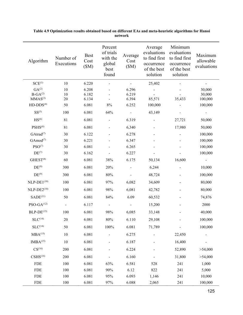
125

Table 4.9 Optimization results obtained based on different EAs and meta-heuristic algorithms for Hanoi network


Best Cost ($M)


found

Average Cost ($M)



Maximum allowable

evaluations

SCE(1) 10 6.220 - - 25,402 - -

GA(2) 10 6.208 - 6.296 - - 30,000 B-GA(2) 10 6.182 - 6.219 - - 30,000

MMAS(3) 20 6.134 - 6.394 85,571 35,433 100,000

HD-DDS(4) 50 6.081 8% 6.252 100,000 - 100,000

SS(5) 100 6.081 64% - 43,149 - -

HS(6) 81 6.081 - 6.319 - 27,721 50,000

PSHS(6) 81 6.081 - 6,340 - 17,980 50,000

GAtrad(7) 30 6.122 - 6.278 - - 100,000

GAmod(7) 30 6.221 - 6.347 - - 100,000

PSO(7) 30 6.081 - 6.265 - - 100,000

DE(7) 30 6.162 - 6.227 - - 100,000

GHEST(8) 60 6.081 38% 6.175 50,134 16,600 -

DE(9) 300 6.081 20% - 6,244 - 10,000

DE(9) 300 6.081 80% - 48,724 - 100,000

NLP-DE1(10) 100 6.081 97% 6,082 34,609 - 80,000

NLP-DE2(10) 100 6.081 98% 6,081 42,782 - 80,000

SADE(11) 50 6.081 84% 6.09 60,532 - 74,876

PSO-GA(12) - 6.117 - - 15,200 - 2000

BLP-DE(13) 100 6.081 98% 6,085 33,148 - 40,000

SLC(14) 20 6.081 80% 6.110 29,108 - 100,000

SLC(14) 50 6.081 100% 6.081 71,789 - 100,000

MBA(15) 10 6.081 - 6.275 - 22,450 -

IMBA(15) 10 6.081 - 6.187 - 16,400 -

CS(16) 200 6.081 - 6.224 - 52,890 >54,000

CSHS(16) 200 6.081 - 6.160 - 31,800 >54,000

FDE 100 6.081 63% 6.581 528 241 1,000

FDE 100 6.081 90% 6.12 822 241 5,000

FDE 100 6.081 95% 6.093 1,146 241 10,000

FDE 100 6.081 97% 6.088 2,065 241 100,000

126

(1) Liong and Atiquzzaman (2004) (2) Reca and Martinez (2006) (3) Zecchin et al. (2006) (4) Tolson et al. (2009) (5) Min-Der et al. (2007) (6) Geem (2013) (7) Marchi et al. (2014) (8) Bolognesi et al. (2010)

(9) Suribabu (2010) (10) Zheng et al. (2011) (11) Zheng et al. (2013) (12) Babu and Vijayalakshm (2013) (13) Zheng et al. (2014) (14) Moosavian and Roodsari (2014) (15) Sadollah et al. (2014) (16) Sheikholeslami et al. (2016)

127

Table 4.10 Optimization results obtained based on different EAs and meta-heuristic algorithms for New York Tunnels network


Best Cost ($M)


found

Average Cost ($M)



Maximum allowable

evaluations

MMAS(1) 20 38.640 60% 38.84 30,711 22,635 50,000

SS(2) 100 38.640 65% - 57,583 - -

HD-DDS(3) 50 38.640 86% - 47,000 - 50,000

HS(4) 81 38.640 - - 5,991 3,373 10,000

PSHS(4) 81 38.640 - - 5,923 4,475 10,000

GAtrad(5) 30 38.640 - 40.99 - - 100,000

GAmod(5) 30 38.640 - 39.013 - - 100,000

PSO(5) 30 38.640 - 39.845 - - 100,000

DE(5) 30 38.640 - 38.667 - - 100,000

GHEST(6) 60 38.640 92% - 11,464 2,100 -

DE(7) 300 38.640 71% - 5,494 3,220 10,000

NLP-DE1(8) 100 38.640 99% 38.64 8,277 - 20,000

NLP-DE2(8) 100 38.640 99% 38.64 10,631 - 20,000

SADE(9) 50 38.640 92% 38.64 6,598 - 9,227

BLP-DE(10) 100 38.640 100% 38.64 3,486 - 7,500

SLC(11) 20 38.640 80% 38.81 7,821 - 100,000

SLC(11) 50 38.640 100% 38.64 15,764 - 100,000

GA(12) 50 38.796 8% 40.96 23,070 - 30,000

PSO(12) 50 38.796 28% 40.82 6,100 - 100,000

ACO(12) 50 38.796 16% 39.24 55,950 - 150,000

MA(12) 50 38.796 30% 39.23 43,482 - 15,000

SFLA(12) 50 38.796 14% 39.51 7,963 - 10,000

FDE 100 38.640 47% 52.87 472 238 1,000

FDE 100 38.640 84% 38.92 1,454 238 5,000

FDE 100 38.640 89% 38.69 1,685 238 10,000

FDE 100 38.640 100% 38.64 4,193 238 100,000

128

(1) Zecchin et al. (2006) (2) Min-Der et al. (2007) (3) Tolson et al. (2009) (4) Geem (2013) (5) Marchi et al. (2014) (6) Bolognesi et al. (2010) (7) Suribabu (2010)

(8) Zheng et al. (2011) (9) Zheng et al. (2013) (10) Zheng et al. (2014) (11) Moosavian and Roodsari (2014) (12) El-Ghandour and Elbeltagi (2017)

129

Table 4.11 parameter values of ten EAs

Algorithm nPop Parameters GA(1) 100 Mutation= 0.01 Crossover= 0.8 SA(2) 100 Initial Temperature =100 Reannealing Interval =100 HS(3) 100 HMCR =0.8 PAR = 0.4 DE(4) 100 Mutation= 0.5 Crossover= 0.3 PSO(5) 100 Inertia Weight = 0.99 Evolution Parameters = 2 ABC(6) 100 Food Number = 50 Limit Trials = 100 SLC(7) 100 Imitation = U(0.2,0.8) Provocation = 1 and 0.5

MEIGO(8) 100 Black Box Optimizer with self adaptive parameters CMAES(9) 100 Sigma = 0.5 Mu = 50

(1) Matlab (2) Matlab (3) Geem (2006) (4) Suribabu 2010 (5) Suribabu and Neelakantan (2006)

(6) Karaboga (2005) (7) Moosavian and Roodsari (2014) (8) Egea et al., (2014) (9) Hansen and Kern (2004)

130

Table 4.12 Least cost solutions for the Farhadgerd network: 1000 function evaluations

1,000 evaluations

Min($M) Max($M) Mean($M) Standard deviation

(M) GA 27.730 32.180 29.500 1.115 SA 29.190 36.670 32.700 2.269 HS 29.210 34.220 31.740 1.374 DE 33.100 36.170 34.750 0.931

PSO 26.170 30.850 28.920 1.410 ABC 32.400 38.110 34.920 1.596 SLC 28.710 34.260 32.030 1.671

MEIGO 21.930 36.280 31.840 4.595 CMAES 45.690 818.800 171.700 225.800

FDE 18.950 30.920 21.800 3.374 Best FDE PSO FDE GA

131


10,000 evaluations


(M) GA 21.300 26.100 22.880 0.994 SA 24.050 34.440 27.940 2.454 HS 22.800 24.600 23.850 0.455 DE 22.100 23.940 23.070 0.427

PSO 22.280 29.220 25.040 1.695 ABC 23.430 27.380 25.330 1.084 SLC 20.070 22.290 20.940 0.565

MEIGO 21.080 24.370 22.740 0.769 CMAES 18.490 19.710 19.060 0.273

FDE 17.920 19.570 18.540 0.540 Best FDE FDE FDE CMAES

132


40,000 evaluations


(M) GA 19.460 23.020 21.080 0.8677 SA 22.750 27.280 24.950 1.327 HS 21.380 22.750 22.240 0.324 DE 19.560 20.610 20.060 0.262

PSO 20.210 26.530 24.070 1.380 ABC 20.830 23.980 22.640 0.805 SLC 17.790 18.730 18.290 0.301

MEIGO 19.090 20.300 19.700 0.335 CMAES 17.840 18.180 18.040 0.0910

FDE 17.780 18.420 17.920 0.209 Best FDE CMAES FDE CMAES

133

Table 4.15 Optimization results obtained based on different EAs and meta-heuristic algorithms for Farhadgerd network


Best Cost ($M)


found

Average Cost ($M)



Maximum allowable

evaluations

SLC 100 17.79 - 18.27 - - 100,000

CMAES 100 17.84 - 18.01 - - 100,000

MEIGO 100 17.98 - 18.92 - - 100,000

DE 100 17.78 30% 17.82 88,590 67,800 100,000

FDE 100 17.78 74% 17.80 24,294 638 100,000

134

Mutation in DE Mutation in FDE

Figure 4.1 Conceptualization of mutation operation for DE and FDE

135

Figure 4.2 Initial solution vectors for f(x,y)=x2+y2 EA benchmark test problem

136

1- De Jong’s Function (Sphere Function)

2-Ackley’s Function

3- Griewangk’s Function

4- Rosenbrock’s Valley

5- Michalewicz’s Function

6-Rastrigin’s Function

7- Schwefel’s Function

8-Sum of Power Functions

Figure 4.3 EA benchmark test problems

-5

0

5

-5

0

50

10

20

30

40

50

-40-20

020

40

-40

-20

0

20

400

5

10

15

20

-1000-500

0500

1000

-1000

-500

0

500

1000-50

0

50

100

150

200

-2-1

01

2

-2

-1

0

1

20

1000

2000

3000

4000

01

23

4

0

1

2

3

4

-2

-1.5

-1

-0.5

0

x 1024

-2-1

01

2

-2

-1

0

1

20

10

20

30

40

50

-500

0

500

-500

0

500-1000

-500

0

500

1000

-1-0.5

00.5

1

-1

-0.5

0

0.5

10

0.5

1

1.5

2

137

1) 2D, DE= 17900, FDE= 6090

2) 2D, DE= 28100, FDE= 8161

3) 2D, DE= 30300, FDE= 16689

4) 2D, DE= 81200, FDE= 10951

5) 2D, DE= 3600, FDE= 970 6) 2D, DE= 15900, FDE= 5039

7) 2D, DE= 15900, FDE= 3095 8) 2D, DE= 7000, FDE= 4660

Figure 4.4 Convergence properties of DE and FDE for EA benchmark test problems, based on two-variable formulations

Ob

ject

ive

fun

ctio

n

Obj

ectiv

e fu

nct

ion

Ob

ject

ive

fun

ctio

n

Ob

ject

ive

func

tion

Ob

ject

ive

fun

ctio

n

Obj

ect

ive

fun

ctio

n

Ob

ject

ive

fun

ctio

n

Obj

ect

ive

fun

ctio

n

138

9)10D, DE= 54400, FDE= 24177

10) 10D, DE= 72200, FDE= 32491

11) 10D, DE= 81700, FDE= 27224 12) 10D, DE= 100,000, FDE= 96962

13) 10D, DE= 29200, FDE= 9690 14) 10D, DE= 58100, FDE= 23758

15) 10D, DE= 28000, FDE= 9707 16) 10D, DE= 20100, FDE= 10551

Figure 4.5 Convergence properties of DE and FDE for EA benchmark test problems, based on ten-variable formulations

0 100 200 300 400 500 600 700 800 900 1000

Number of iteration

10-20

10-15

10-10

10-5

100

105

DEFDE

0 100 200 300 400 500 600 700 800 900 1000

Number of iteration

-9

-8

-7

-6

-5

-4

DEFDE

0 100 200 300 400 500 600 700 800 900 1000

Number of iteration

10-15

10-10

10-5

100

105

DEFDE

0 100 200 300 400 500 600 700 800 900 1000

Number of iteration

-4000

-3500

-3000

-2500

-2000

-1500 DEFDE

0 100 200 300 400 500 600 700 800 900 1000

Number of iteration

10-200

10-150

10-100

10-50

100

DEFDE

139

Chapter 5 : A Fuzzy Programming Approach for Multi-Objective

Optimization of Water Distribution Systems

5.1 Preface

As mentioned in Chapters 1 and 3, the resilience index can be applied to implicitly assess reliability

of WDN design. It is defined as the capability of system to “bounce back” following some failure

and can be approximated as the capacity of a network to absorb disturbance while experiencing

alterations, so as to retain essentially the same function, structure, identity, and feedback

information. In Chapter 3, a nondominated sorting population-based multi-objective design

framework, based on the minimization of cost and maximization of the resilience index, is

presented. Maximization of the resilience index increases the hydraulic reliability of the system.

For enhancing both mechanical and hydraulic reliability in WDN design, researchers propose

several additional reliability surrogates. These include: (1) the sum over all nodes of the relative

surplus of energy at each node; (2) the minimum surplus head at a critical node; (3) the sum over

all nodes of the relative surplus of energy at each node modified by the degree of pipe diameter

uniformity of its associated loop; and (4) the minimum pipe diameter uniformity of the associated

loops over all nodes. For employing these surrogates, this chapter proposes a fuzzy multi-objective

programming model for meeting more than three competing objectives in the optimal design of

WDNs. FM functions for minimizing the pipe network cost and maximizing the reliability

surrogates are defined, and the model maximizes the degree of satisfaction of these membership

functions. Based on post-optimization cut-set analyses, the proposed model that minimizes cost

and maximizes the resilience index and the minimum pipe diameter uniformity of the associated

loops over all nodes, exhibits the highest level of mechanical reliability. Unlike the nondominated

multi-objective models discussed in Chapter 3 which provide populations of solutions on the

Pareto optimal frontier, the fuzzy programming model converges to only one good compromise

solution.

5.2 Abstract

This paper proposes a fuzzy multi-objective programming model for meeting competing objectives

in the optimal design of water distribution systems (WDSs). Fuzzy membership functions for

minimizing the pipe network cost and maximizing a number of reliability surrogates are defined,

and the model maximizes the degree of satisfaction of these membership functions. Reliability

140

surrogates investigated include: i) the sum over all nodes of the relative surplus of energy at each

node; ii) the minimum surplus head at a critical node; iii) the sum over all nodes of the relative

surplus of energy at each node modified by the degree of uniformity of its associated loop; and iv)

the minimum uniformity of the associated loops over all nodes. The model is applied to various

combinations of objective functions, to identify the design pipe diameters of the water-main

network of Farhadgerd, Iran. Optimal solutions of the various model formulations show that for

this WDS the third surrogate (iii) may be a reasonable substitute for the first surrogate (i), and that

while the inclusion of the last surrogate (iv) may be beneficial, the inclusion of the second

surrogate (ii) may not. Based on post-optimization cut-set analyses, the model that minimizes cost

and maximizes surrogates (iii) and (iv) exhibits the highest level of mechanical reliability, while

the model that minimizes cost and maximizes the second surrogate (ii) exhibits the lowest level of

mechanical reliability.

5.3 Introduction

In optimal design of water distribution systems (WDSs), network components are selected

considering the system cost of construction and operation and the ability of the network to satisfy

consumer demands for water availability, pressure, and quality, under normal and abnormal

operating conditions, including during pipe bursts and as components deteriorate. Hydraulic

reliability is a representative measure of the ability of the system to respond to gradual changes in

the system characteristics, e.g., available pipe diameters and pipe roughness, and short or long-

term shifts in consumption, e.g., hourly variations in withdrawal rates or community-driven

changes in required fire flows (Shamir and Howard 1981). Mechanical reliability is a measure of

the ability of the system to adapt to mechanical failures, e.g., to maintain operating goals during

pipe, valve, or pump failures (Mays 1989). Approaches for accounting for reliability include

stochastic analysis of uncertainty regarding the condition of network components (Damelin et al.

1972) and the level of system demands (Mays and Cullinane 1986), and the estimation of

deterministic surrogate measures of reliability (Todini 2000). The latter approach has gained wide

recognition in recent years due to the ease with which the surrogates may be incorporated as

constraints or objectives in optimization models and to advances in Computational capabilities for

solving these models (Babayan et al. 2005; Giustolisi et al. 2009; Schwartz et al. 2016).

141

Surrogates of hydraulic reliability include the: relative surplus of pressure head over all system

nodes and the minimum surplus head at a critical node, as introduced by Todini (2000),

modifications of the former approach as a function of the degree of uniformity of the network

loops (Prasad and Park 2004), minimum flow entropy (Ang and Jowitt 2003; Atkinson et al. 2014),

or variations and combinations of these (Saleh and Tanyimboh 2014; Jayaram and Shrinivasan

2008; Ostfeld et al. 2014; Creaco et al 2016). While similar surrogates have been proposed (Todini

2000; Geem 2015), the most widely used approach for estimating mechanical reliability is a cut-

set analysis in which a given design is evaluated based on the number of single pipes that could be

removed from operation without causing the network design to fail to meet specified nodal

pressures. This approach exacts a high computational burden because every possible pipe removal

scenario requires a re-evaluation of the hydraulic conditions, and thus it is generally undertaken

post-optimization.

Recent progress in WDS optimization successfully applies multi-objective evolutionary

algorithms for evaluating the cost-reliability Pareto Optimal Frontier (Prasad et al. 2003; Farmani

et al. 2005a; Farmani et al. 2006; Raad et al. 2009; Baños et al. 2010; Greco et al. 2012). The most

attractive of these algorithms use nondominated sorting in the selection process, e.g., the modified

nondominated sorting genetic algorithm, NSGA-II (see Farmani et al. 2006), the nondominated

sorting differential evolution algorithm, NSDE, and the nondominated sorting differential

evolution algorithm with ranking-based mutation operator, NSDE-RMO (for the latter two, see

Moosavian and Lence 2016), to identify well-distributed solutions along the entire cost-reliability

domain. Typically, a large number of Pareto optimal solutions are generated, though generally

only a small set of these are evaluated in depth for mechanical reliability (Farmani et al 2005a),

and no standard approach for selecting which WDS solutions to investigate has been adopted.

Several approaches for incorporating decision-making preferences to identify WDS solutions that

achieve the best compromise among the objectives have been proposed (Vamvakeridou et al. 2006;

Atiquzzaman et al. 2006), although these approaches are generally challenged as the number of

solutions and objectives, and the complexity of the WDS, are increased.

Considered an appropriate framework for representing imprecise information and linguistic

ambiguity, fuzzy set theory (Zadeh 1965) has been applied in the design and operation of WDSs

to describe uncertain conditions such as nodal demands and pipe roughness information, and

system constraints such as desirable pressure head and velocity levels. Fuzzy programming

142

models for WDS optimization comprised of fuzzy constraints (Goulter and Bouchart 1988; Xu and

Goulter 1999; Bhave and Gupta 2007; Xu and Qin 2013) and objective functions that account for:

a single fuzzy benefit or weighted benefits (Vamvakeridou et al. 2006; Geem, 2015), the degree

of satisfaction of fuzzy constraints through penalty functions (Amirabdollahian et al. 2011), and

the probability of meeting fuzzy constraints (Fu and Kapelan 2011), have been investigated. The

findings of these studies indicate that, by accounting for uncertainty in the system limitations and

goals, fuzzy programming models may lead to improved WDS designs that are robust to changes

in system conditions.

We present a mixed-integer fuzzy programming model for identifying the WDS design solutions

that minimize cost while maximizing one or more surrogates for hydraulic reliability, and

implement this model with the Soccer League Competition Algorithm, SLC (Moosavian and

Roodsari 2014a), an evolutionary algorithm for which the decision variables may take any form.

This approach defines fuzzy membership functions for each of the objectives and maximizes the

degree of satisfaction of all membership functions. Attractive solutions are identified directly,

without the need to generate the entire Pareto Optimal Frontier. By maximizing the satisfaction

of the various fuzzy objectives, it is possible to substantially increase the probability of finding an

attractive compromise among them. Depending on the composition of the objective set, a number

of compromise solutions on the Pareto Optimal Frontier may be identified, and post-optimization

analysis of mechanical reliability for these points may be used as comparators, or in conjunction

with other information, to evaluate the potential performance of a given WDS design.

The following section presents the general model for maximizing membership of fuzzy objectives

for cost and reliability. This model may be extended for any number of objectives, and thus may

include a number of surrogates for reliability. Next, the objectives for designing WDSs applied

in this paper, and the mixed-integer WDS fuzzy optimization model are described. In Section 4,

the SLC is briefly described in the context of the WDS optimization problem. Finally, the

application of the fuzzy programming model for finding compromise solutions for design of the

water-main network for the town of Farhadgerd, Iran is provided, post-optimization cut-set

analyses are conducted for these solutions, and ideal solutions for these multi-objective problems

are computed and compared with the fuzzy programming results.

143

5.4 Fuzzy Programming for Multi-objective Optimization of Cost and Reliability

Most multi-objective optimization approaches fall into three categories, approaches that: i) identify

the nondominated trade-offs between objectives, or the Pareto Optimal Frontiers; and identify the

solution which best meets all objectives, or an attractive compromise solution on the Pareto

Optimal Frontier, either with (ii); or without (iii) considering the preferences of the decision

makers, or the welfare of the users (Cohen 1978). Our fuzzy programming model for multi-

objective WDS problems is an example of the latter category. Here, the best compromise WDS

design for the competing objectives of cost and reliability maximizes the satisfaction of fuzzified

values of these objectives, expressed as linear fuzzy membership functions. By expressing the

objectives in a fuzzified manner, it is possible to further explore, or stretch, the Pareto Optimal

Frontier, so as to increase the potential for finding the most attractive compromise solution. While

different fuzzy membership functions exist, linear functions in which the maximum membership

represents the best possible value for a given objective, and the minimum membership the worst,

are used here. If the resulting cost and reliability for a given set of decisions, x, (i.e., the diameter

of pipe selected for each pipe of the network) are defined as Cost(x) and Reliability(x), and the

minimum and maximum possible values of cost and reliability are defined as Costmin, and Costmax,

and Reliabilitymin, and Reliabilitymax, respectively, the linear membership function for the cost

objective is a normalized cost function, for costs that range from Costmin to Costmax, and is defined

as a function of discrete variables as follows:

max

maxmin

min

minmax

max1 ,

0

1

CostxCostif

CostxCostCostif

CostxCostif

CostCost

xCostCostxCost

(5.1)

And similarly, the membership function of the reliability objective is a normalized reliability

function, for reliability levels that range from Reliabilitymin to Reliabilitymax, and is defined as a

function of discrete variables as follows:

max

maxmin

min

minmax

min2

ee

eee

ee

,

1ee

ee0

e

liabilityRxliabilityRif

liabilityRxliabilityRliabilityRif

liabilityRxliabilityRif

liabilityRliabilityR

liabilityRxliabilityRxliabilityR

(5.2)

144

Using Zimmermann’s minimum operator (Zimmermann 1991), the general multi-objective model

for optimizing cost and reliability, as a function of discrete variables, is as follows:

𝑀𝑖𝑛 𝜇 𝐶𝑜𝑠𝑡 𝑥 , 𝑎𝑛𝑑 𝑀𝑎𝑥 𝜇 𝑅𝑒𝑙𝑖𝑎𝑏𝑖𝑙𝑖𝑡𝑦 𝑥

Subject to:

𝑔 𝑥 0 𝑓𝑜𝑟 𝑗 1,2, … , 𝑚

𝑥 0 𝑓𝑜𝑟 𝑡 1,2, … , 𝑇

(5.3)

(5.4)

(5.5)

where 𝑔 𝑥 = jth constraint function and 𝑥 = tth decision variable.

According to Zimmermann (1991), this model may be solved by introducing an auxiliary

continuous variable, λ, known as the overall satisfaction, which ranges from 0 to 1, and by

transforming Eq. 5.3-5.5 into the equivalent single objective mixed-integer optimization problem

of maximizing λ. The transformed problem finds the intersection of the fuzzy member functions

of the objectives (Eq. 5.1-5.2) at a point that maximizes the level of satisfaction of the fuzzy

membership function for each of the objectives. It is:

𝑀𝑎𝑥 𝜆

Subject to:

𝜇 𝐶𝑜𝑠𝑡 𝑥 𝜆

𝜇 𝑅𝑒𝑙𝑖𝑎𝑏𝑖𝑙𝑖𝑡𝑦 𝑥 𝜆

0 𝜆 1

(5.6)

(5.7)

(5.8)

(5.9)

and Eqs (5.4) and (5.5) above.

145

5.5 Multi-objective Optimization of Water Distribution Systems (WDSs)

For purposes of this paper, the WDS decisions to be made are limited to the selection of pipe sizes,

while pipe layout and connectivity, nodal demands, and minimum head requirements are imposed.

The objective of minimizing the cost of a WDS design may be expressed as:

𝑀𝑖𝑛 𝐶𝑜𝑠𝑡 𝐶𝑜𝑠𝑡 𝐷 𝐿 (5.10)

where Li = length of each pipe (meters); Costi (Di) = cost of a pipe of a given diameter ($/meter);

Di = diameter of the selected pipe (meters); and np = number of pipes.

Among the possible surrogates proposed for estimating the reliability of pipe networks, the most

widely used surrogate is the resilience index (Ir) introduced by Todini (2000), which characterizes

the intrinsic capability of the system to overcome failures while still satisfying demands and

pressures in nodes. The objective of maximizing the reliability of a WDS design is expressed as:

𝑀𝑎𝑥 𝐼𝑟 ∑ 𝑞 𝐻 𝐻

∑ 𝑄 𝐻 ∑ 𝑃𝛾 ∑ 𝑞 𝐻

(5.11)

where nn = number of nodes; no = number of reservoirs; qk = flow demand at node k

(meters3/second); Hk = available pressure head at node k (meters); 𝐻 = minimum pressure head

required at all nodes (meters); Qk = supply at a reservoir located at node k (meters3/second); H0k =

elevation head of a reservoir located at nPode k (meters); and Pi = power of a pump located in pipe

i (watts); γ = specific weight of water (Newtons/ meters3). Being the ratio of the energy available

in the network to that required, Ir ranges from 0 to 1.

Another important indicator introduced by Todini is the minimum surplus head (Is), which is

defined as the smallest nodal pressure head difference between the minimum required and

observed pressure. Farmani et al. (2005a) found that increasing the value of this index can improve

mechanical reliability. The objective function based on this measure is formulated as:

𝑀𝑎𝑥 𝐼𝑠 𝑀𝑎𝑥𝑀𝑖𝑛 𝐻 𝐻 , 𝑘 1, … , 𝑛𝑛 (5.12)

Prasad and Park (2004) introduced the network resilience index (NRI), which incorporates the

effects of both surplus power and reliable loops. Reliable loops can be ensured if the pipes

146

connected to a node do not vary greatly in diameter. If the uniformity of pipes connected to a node

k is defined as Ck, the objective function for the NRI, is formulated as:

𝑀𝑎𝑥 𝑁𝑅𝐼 ∑ 𝐶 𝑞 𝐻 𝐻

∑ 𝑄 𝐻 ∑ 𝑃𝛾 ∑ 𝑞 𝐻

(5.13)

where

𝐶∑ 𝐷

𝑛𝑘 ∗ max 𝐷

(5.14)

where nk = number of pipes connected to node k, and Dik = diameter of each of the nk pipes

connected to node k.

As a fourth surrogate, we propose a version of NRI, which seeks to maximize the least uniformity

of pipes over all nodes as a means of potentially improving mechanical reliability. That is, the

more uniform the loops, the more likely they are to be able to reroute flow during unforeseen pipe

closures. The objective function for this surrogate is:

𝑀𝑎𝑥 𝐼𝑑 𝑀𝑎𝑥𝑀𝑖𝑠 𝐶 𝑀𝑎𝑥𝑀𝑖𝑛∑ 𝐷

𝑛𝑘 ∗ max 𝐷

(5.15)

Since the design pipe sizes must be selected from those commercially available, the fuzzy

transformed optimization model of the WDS design problem is a mixed-integer problem:

𝑀𝑎𝑥 𝜆

Subject to:

𝑄 𝑄 𝑞 , ∀ 𝑘 𝜖 𝑛𝑛

ℎ𝑓

∆𝐻, ∀ 𝑙 𝜖 𝑛𝑙

𝐻 𝐻 , ∀ 𝑘 𝜖 𝑛𝑛

𝐷 𝐷 1 , 𝐷 2 , … , 𝐷 𝑆 , ∀ 𝑖 𝜖 𝑛𝑝

𝜇 𝐶𝑜𝑠𝑡 𝑥 𝜆

(5.16)

(5.17)

(5.18)

(5.19)

(5.20)

(5.21)

147

𝜇 𝐼𝑟 𝑥 𝜆

𝜇 𝐼𝑠 𝑥 𝜆

𝜇 𝑁𝑅𝐼 𝑥 𝜆

𝜇 𝐼𝑑 𝑥 𝜆

0 𝜆 1

(5.22)

(5.23)

(5.24)

(5.25)

(5.26)

where Qin and Qout = flow into and out of node k (meters3/second), respectively; hfi = head loss

due to friction in the pipe i (meters) computed by the Hazen-Williams or Darcy-Weisbach

formulae; nl = loop set; ∆H = 0, if the path is closed, and ∆H = difference between nodal heads

at both reservoirs (meters), if the loop is between two fixed head reservoirs; and S = the number

of candidate diameters commercially available.

Eq. (5.17) represents the continuity constraint for each node in the network. Eq. (5.18) represents

the conservation of energy constraint for each loop in the network, that is, the total head loss around

a closed loop should be equal to zero, or the head loss along a loop between the two fixed head

reservoirs should be equal to the difference in water level of the reservoirs. Eq. (5.19) constrains

the pressure head at each node to be greater than the prescribed minimum pressure head. Eq. (5.20)

requires that the diameter of the pipes selected be commercially available, and Eqs (5.21)-(5.26)

are analogous to Eqs (5.7)-(5.9) for the case where all four surrogates for hydraulic reliability are

considered simultaneously.

The Hazen-Williams formula which defines the pressure head loss equation for pipe i connecting

nodes n and m is:

(5.27)

where Qi = the flow in the pipe i (meters3/second); and CHi = Hazen-Williams coefficient for pipe

i. Thus Eq. (5.16)-(5.27) generate a unique compromise Pareto-optimal solution for the multi-

objective WDS problem and this problem may be solved with any powerful mixed-integer

programming algorithm.

0.852

ii4.871i

1.852iimni QQDCHL10.667HHhf

148

5.6 Soccer League Competition (SLC) Algorithm

Given the non-linearity and non-convexity of the multi-objective WDS design problem and the

implicit constraints requiring hydraulic simulation to satisfy the WDS continuity and energy

equations (Eq. 5.17 and 5.18), we apply the SLC evolutionary algorithm with mixed-integer

solution vectors. The SLC algorithm has successfully achieved high performance in optimization

of discrete problems, such as WDS design (Moosavian and Roodsari 2014b), knapsack problems

(Moosavian 2015) and the set-covering problem (Jaramillo et al. 2016), though it can also

accommodate continuous and mixed-integer variables.

The SLC algorithm is inspired from professional soccer leagues. It involves different teams, or

collections of solutions, where each solution is a team member, and a number of operators that act

on the team members to perform an effective search for finding the near optimal solution. For the

network optimization problem each of the team members, or solutions, may comprise the set of

design pipe diameters for the system.

The key organizing structure of the algorithm is the soccer teams, and each team includes fixed

players (FPs), or fixed sets of pipe diameter solution vectors, and substitute players (Ss), or

substitute sets. The number of fixed players, nFP, and the number of substitute players, nS, is

equivalent for all teams. The power of each team member, is calculated based on its objective

function value. For minimization problems, e.g., that minimize the design cost of a network, the

power of player j on team i, PP(i,j) is the inverse of its objective function value. The players are

rank ordered as a function of their power, and the nFP players with the highest power are

considered to be the fixed players, while the nS players with the lowest power are considered to

be substitutes. The power of a team is the average power of the fixed players of the team, i.e.:

(5.28)

nFPTP i 1 nFP PP(i , j)

j 1

where TP(i) = the power of team i.

The algorithm mimics matches between teams and determines the winners based on their relative

power, and the winner of a match has a higher probability of increasing its power for future

matches. After each match, all players (decision vectors) on the winning team undergo operations

that change their decisions, and thus their power (i.e., strengthen or weaken each player),

149

producing modified team members. Finally, the original strength of each player on this winning

team is compared with its modified strength and the player, i.e., decision vector, with the greater

strength, is allowed to play on the team in the next match.

A round is defined as a set of matches that allows each team, or modified team, to play with each

other team in the league. If NT is the number of teams in the league, at each round of the tournament

the number of matches is:

𝑁𝑇 𝑁𝑇 12

(5.29)

After finishing of the total matches in a given round, all players in the league are re-sorted in

descending order of their power and are assigned to teams. The nFP highest ranked players are

assigned to team one, the next nFP highest ranked players are assigned to team two, and so on

until all NT×nFP fixed players are assigned to a team. And finally, the next nS highest ranked

players are assigned to team one, and the next nS highest ranked are assigned to team two, and so

on until all NT×nS substitute players are assigned to a team.

Thereafter, the next round is played with these new teams. The user specifies the stopping criteria

to be either based on a limit of the number of rounds undertaken, or the number of function

evaluations made (in this paper, the limit on the number of function evaluations is set to be 106).

Details of the algorithm are described in Moosavian and Roodsari (2014a and 2014b).

5.7 Fuzzy Multi-objective Optimization of the Farhadgard WDS

Hydraulic simulation to satisfy the energy and continuity equations for each SLC solution vector

is undertaken with the Global Gradient Algorithm (GGA) (Todini 2000), and the linked

simulation-optimization process is implemented in MATLAB. Fuzzy multi-objective optimal

solutions to the cost-reliability WDS design problem are examined for a variety of surrogates for

reliability, for a water supply network serving a population of approximately 8200 in the town of

Farhadgard, Iran, a residential community near the city of Mashhad. Post-optimization cut-set

analyses are also undertaken as a means of further evaluating the mechanical reliability of these

design solutions. The Farhadgard network (Figure 5.1) comprises 68 pipes, 53 nodes, and two gate

valves. The network has one reservoir with a head of 510 m and the minimum pressure required

in the network is 20 m. Other information regarding the hydraulic simulation of this network is

provided in Moosavian and Jaefarzadeh (2014).

150

5.7.1 Hydraulic Reliability

Table 5.1 presents the objective function values for cost and reliability for the minimum cost,

maximum cost, and fuzzy multi-objective optimal models with a variety of objectives. The

minimum cost model for this network, considers cost as the sole objective function (i.e., Eqs (5.10),

and (5.17)-(5.20) and represents the solution with the least reliability. The maximum cost solution,

for which all pipe diameters are set to their largest possible values, represents the solution with the

overall maximum reliability. These solutions provide the range of possible values for cost and each

of the reliability surrogates. When two objectives are considered, i.e., cost and any one of the

reliability surrogates, the relative value of reliability surrogate increases significantly with only

moderate increases in the relative design cost. The fuzzy Cost+Ir and Cost+NRI models provide

nearly the same results for the Ir surrogate (0.5940 and 0.5900) and the NRI surrogate (1.907 and

2.01), though the Cost+NRI model results in a somewhat higher cost. This indicates that the NRI

may be a reasonable substitute for the Ir surrogate. The optimal pipe diameters for these two

models for pipe numbers 1-68 are similar, as shown in Figure 5.2. The fuzzy Cost+Ir, Cost+NRI,

and Cost+Is models all result in significantly improved values for the Is surrogate (1.907, 2.010,

and 2.850, relative to its range of from 0.015 to 2.99), indicating that this measure may be well

represented by the inclusion of Ir or NRI surrogates. In contrast, the results of all of the fuzzy two-

objective models indicate that the only way to assure that the Id surrogate increases from its lowest

value of 0.0638 is to account for it explicitly in the objective function set. The Id surrogate

describes the uniformity of the diameters at a given node, or entering a given junction, for all

nodes/junctions in the network. Unlike Ir, NRI, or Is, it does not include energy considerations

between nodes or discharge requirements at nodes. The increase in the value of the Id surrogate to

0.279 in the fuzzy Cost+Id model solution is accompanied by corresponding decreases in all

reliability surrogates and an increase in the cost. The significant difference in pipe diameters

induced by including the Id surrogate is illustrated in Figure 5.3, which provides optimal pipe

diameters for the Cost+Ir and Cost+Id models.

Thus, solutions for models that contain only select sets of objectives, the fuzzy Cost+Ir+Is,

Cost+NRI+Is, Cost+Ir+Id, Cost+NRI+Id, Cost+Ir+Id+Is, and Cost+NRI+Id+Is models, are

examined further. The solution of the fuzzy Cost+Ir+Is model shows that, relative to the fuzzy

Cost+Ir model, the addition of the Is surrogate results in an improved value of Is (from 1.9070 to

2.6233), with an accompanying increase in cost and very little change in the other reliability

151

surrogates. As expected, given the similarities of the fuzzy Cost+Ir and Cost+NRI models, similar

results are observed for the fuzzy Cost+NRI and Cost+NRI+Is models where the Is surrogate is

improved from 2.010 to 2.373, and very little change occurs in all other reliability surrogates. As

was observed for the two-objective fuzzy models, the value of the Id surrogate may only be

improved by including this objective explicitly in the fuzzy model. For the fuzzy Cost+Ir+Id and

Cost+NRI+Id models the increase in the value of the Id surrogate is accompanied by corresponding

decreases in all reliability surrogates and an increase in the cost. Again, the addition of the Is

surrogate as an objective in the fuzzy Cost+Ir+Id+Is and Cost+NRI+Id+Is models serves only to

improve the Is surrogate (from 1.244 to 1.978, and from 0.740 to 1.791, respectively), with an

accompanying increase in cost, and very little change in the other reliability surrogates.

5.7.2 Mechanical Reliability

Table 5.2 provides the results of the post-optimization cut-set analyses for these models, where

columns 2-4 provide the number of individual pipes that may be closed while maintaining pressure

heads of 0, 10 and 20 m throughout the network, and columns 5-7 provide the percentage of the

68 pipes in the network that the cut-set represents. The cut-set analysis of the maximum cost

(maximum diameter) solution has the highest level of mechanical reliability, where 64 of the 68

pipes may be damaged without shortfalls in pressure requirements. Pipe number 1 connected to

the reservoir source and is crucial for operation of the network. Three additional dendritic pipes

(pipe numbers 46, 48 and 51), are critical to the mechanical reliability of the network, and should

any one of these pipes fails, the network will fail to meet the pressure requirements at the extreme

junction for the given pipe. As expected, the minimum cost solution has the lowest level of

mechanical reliability, where only 35, 24, and 4 pipes may be removed while still meeting pressure

head targets of 0, 10, and 20 m, respectively. Among the two-objective models, the fuzzy

Cost+NRI model results in the highest mechanical reliability (with cut-sets comprised of 51, 47,

and 40 pipes for pressure head targets of 0, 10, and 20 m, respectively) and the addition of the Is

surrogate to this model results in a decrease in the mechanical reliability (with cut-sets comprised

of 45, 45, and 39 pipes for pressure head targets of 0, 10, and 20 m, respectively). The fuzzy

Cost+NRI+Id model has the highest mechanical reliability among all fuzzy multi-objective models

(with cut-sets comprised of 54, 51, and 47 pipes, for pressure head targets of 0, 10, and 20 m,

respectively), though the fuzzy Cost+Ir+Id model has nearly the same mechanical reliability, with

cut-sets comprised of 53, 52, and 43 pipes, for pressure head targets of 0, 10, and 20 m,

152

respectively. Maximization of the NRI or Id surrogate favors solutions in which the diameters of

pipes connected to any given junction are as similar as possible, thus the satisfaction of demands

at the junctions is less likely to be dependent on any one pipe. Maximization of the Ir or NRI

surrogate maximizes the total energy available to the network. These two features explain the high

mechanical reliability of the fuzzy Cost+NRI, Cost+Ir+Id, and Cost+NRI+Id models. High

uniformity among pipes at a junction increases the uniformity of the pipes in the entire network,

thus reducing stress on any one pipe, without sacrificing the satisfaction of discharge and pressure

requirements. The slight difference in the mechanical reliability between the Cost+Ir+Id and

Cost+NRI+Id models may be attributed to the difference in the optimal pipe diameters selected,

see Figure 5.4.

The sensitivity of the mechanical reliability to increasing demands is analyzed by performing cut-

set analyses assuming a 10% increase in demands at all nodes (Table 5.3). Again, the maximum

cost and minimum cost solutions represent the highest and lowest mechanical reliability, though

the minimum cost solution is the least robust of all solutions to changes in demand. Among the

two-objective models, the fuzzy Cost+Ir and Cost+NRI models are the most robust to changes in

demands, and the fuzzy Cost+Is and Cost+Id models are the least robust. Since all of the three-

and four- objective fuzzy models include either Ir or NRI, they are all robust to changes in demand.

The fuzzy Cost+Ir+Id and Cost+NRI+Id models again have the highest mechanical reliability

among all fuzzy multi-objective models (with cut-sets comprised of 52, 49, and 37 pipes, and 54,

49, and 36 pipes, respectively, for pressure head targets of 0, 10, and 20 m, respectively).

5.7.3 Comparison with Compromise Set Ideal Solution

As a comparison with the fuzzy programming-based compromise solutions, we evaluate the

compromise solution of the WDS multi-objective problem using the compromise set solution

approach as defined by Yu (1973) and Zeleny (1974a; 1974b). Here, the constraints to the problem

are defined as in Eqs (5.17)-(5.20), and the objective function minimizes the distance from the

ideal solution (minimum cost or maximum reliability) for each of the objectives of the multi-

objective model according to the following relationship:

1

1

*

KK

kkkkkk xZZdMin

(5.30)

153

where dα = minimum distance to the ideal solution; Zkk* = ideal solution for objective kk; Zkk(x) =

optimal solution for objective kk; KK = number of objectives; and α = metric between one and

infinity.

When α is one, Equation 28 gives the absolute deviations from the ideal, and when α is infinity,

only the largest deviation is considered. Yu (1973) shows that, in general, the best-compromise

solutions define a subset of the non-inferior set, for which α ranges from one to infinity.

For purposes of this comparison, we evaluate the compromise solution for a midpoint between

these values, at α equal to two. Tables 5.4 and 5.5 provide the objective function values, hydraulic

reliability, and cut-set analyses (mechanical reliability) for this model. In general, the model

solutions shown in Table 5.4 are different and non-inferior to analogous solutions for the fuzzy

programming models (Table 5.1). However, except for the fuzzy Cost+Is model, the fuzzy

programming models demonstrate a significantly higher mechanical reliability than models based

on a compromise objective function with α equal to two. For more examples of the use of the

compromise set solution approach, i.e., Eq. 30, see Cohen (1978).

5.8 Conclusions

The fuzzy multi-objective WDS model presented in this paper provides a framework for

investigating an assortment of design objectives and for identifying attractive options among these.

An advantage of this modeling framework is that it may be used to identify compromise solutions

that may be investigated in greater detail, e.g., with cut-set analyses. The benefits of this feature

increase as the number of objectives increase, i.e., when the dimensions of the objective space

increase.

The model is applied for evaluating combinations of objectives for minimizing cost and

maximizing reliability, and demonstrated for designing the water-main network of Farhadgerd,

Iran. Among several surrogates for reliability, the NRI and the proposed Id surrogates favor

solutions in which the diameters of pipes connected to any given node are as similar as possible,

and thus are robust to pipe failures. The Ir and NRI surrogates maximize the total energy available

to the network, and are shown to be reasonable substitutes for each other. Post-optimization cut-

set analyses indicate that the most effective objective combinations for assuring mechanical

reliability are the fuzzy Cost+NRI+Id and Cost+Ir+Id models. Both models are also robust to

realistic (+10%) changes in demand. In contrast, the Is surrogate may be well represented by the

154

Ir or NRI surrogates, and is likely redundant. Furthermore, all cut-set analyses indicate that sole

consideration of the Is surrogate, along with cost, result in low mechanical reliability.

As more objectives are identified, e.g., new expressions for reliability, they may be easily added

to the model with little additional programming and computational burden. The modeling

framework is flexible, even in cases where additional simulations may be required, e.g., in

considering water quality in the network as a system objective. A natural extension of the fuzzy

multi-objective model is to fuzzify the constraints (e.g., Equations 17, 18 and 27) to account for

uncertainties in nodal demands and pipe roughness information.

The advantage of the NRI surrogate is that it enhances mechanical reliability by incorporating the

effects of both surplus energy and reliable loops. The results of this paper show that inclusion of

the Id surrogate, which optimizes the uniformity of the loops, further improves mechanical

reliability. Future work will investigate the benefit of applying these surrogates in the optimization

of larger and more complex WDSs.

155

Table 5.1 Fuzzy Multi-objective WDN Solutions for Town of Farhadgerd

Objective Function Values Objective Functions Included

Cost ($) Ir Is NRI Id

Minimum Cost 1.78E+07 0.017 0.015 0.015 0.064 Maximum Cost 7.32E+07 0.066 2.990 0.066 0.400

Cost+Ir 2.15E+07 0.059 1.907 0.044 0.064 Cost+Is 1.92E+07 0.022 2.850 0.019 0.064

Cost+NRI 2.35E+07 0.059 2.010 0.055 0.064 Cost+Id 2.77E+07 0.031 0.352 0.025 0.279

Cost+Ir+Is 2.23E+07 0.058 2.623 0.043 0.064 Cost+NRI+Is 2.42E+07 0.059 2.373 0.054 0.064 Cost+Ir+Id 2.78E+07 0.049 1.244 0.033 0.279

Cost+NRI+Id 2.89E+07 0.054 0.740 0.046 0.264 Cost+Ir+Id+Is 2.87E+07 0.047 1.978 0.035 0.264

Cost+NRI+Id+Is 2.90E+07 0.054 1.791 0.045 0.264

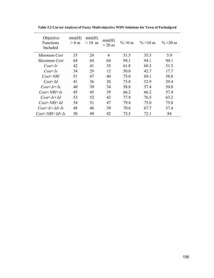
156

Table 5.2 Cut-set Analyses of Fuzzy Multi-objective WDN Solutions for Town of Farhadgerd

Objective Functions Included

min(H) > 0 m

min(H) > 10 m

min(H) > 20 m

% >0 m % >10 m % >20 m

Minimum Cost 35 24 4 51.5 35.3 5.9 Maximum Cost 64 64 64 94.1 94.1 94.1

Cost+Ir 42 41 35 61.8 60.3 51.5 Cost+Is 34 29 12 50.0 42.7 17.7

Cost+NRI 51 47 40 75.0 69.1 58.8 Cost+Id 41 36 20 75.0 52.9 29.4

Cost+Ir+Is 40 39 34 58.8 57.4 50.0 Cost+NRI+Is 45 45 39 66.2 66.2 57.4 Cost+Ir+Id 53 52 43 77.9 76.5 63.2

Cost+NRI+Id 54 51 47 79.4 75.0 75.0 Cost+Ir+Id+Is 48 46 39 70.6 67.7 57.4

Cost+NRI+Id+Is 50 49 42 73.5 72.1 84

157

Table 5.3 Cut-set Analyses of Fuzzy Multi-objective WDN Solutions with 10% Increase in Demands

min(H) > 0 m

min(H) > 10 m

min(H) > 20 m

% >0 m % >10 m % >20 m

Minimum Cost 28 0 0 41.2 0 0 Maximum Cost 63 63 63 92.6 92.7 92.7

Cost+Ir 42 40 31 61.8 58.8 45.6 Cost+Is 29 13 0 42.7 19.1 0

Cost+NRI 48 43 38 70.6 63.2 55.9 Cost+Id 40 31 1 58.8 45.6 1.5



Cost+NRI+Id+Is 50 47 34 73.5 69.1 50

158

Table 5.4 Compromise WDN Solution, with α = 2, for Town of Farhadgerd

Objective Function Values


Cost ($) Ir Is NRI Id

Cost+Ir 1.82E+07 0.035 0.088 0.025 0.064 Cost+Is 1.97E+07 0.025 2.979 0.020 0.064

Cost+NRI 1.83E+07 0.031 0.066 0.026 0.064 Cost+Id 2.06E+07 0.017 0.018 0.014 0.176

Cost+Ir+Is 1.93E+07 0.025 2.978 0.020 0.064 Cost+NRI+Is 1.91E+07 0.024 2.976 0.020 0.064 Cost+Ir+Id 2.05E+07 0.022 0.071 0.019 0.176

Cost+NRI+Id 2.04E+07 0.020 0.318 0.017 0.176 Cost+Ir+Id+Is 2.00E+07 0.023 2.971 0.020 0.143

Cost+NRI+Id+Is 2.10E+07 0.027 2.990 0.023 0.158

159

Table 5.5 Cut-set Analysis of Compromise WDN Solution, with α = 2, for Town of Farhadgerd


min(H) > 0 m

min(H) > 10 m

min(H) > 20 m

% >0 m % >10 m % >20 m

Cost+Ir 42 36 25 61.8 52.9 36.8 Cost+Is 35 29 15 51.5 42.7 22.2

Cost+NRI 40 36 16 58.8 52.9 23.5 Cost+Id 34 21 0 50.0 30.9 0.0



Cost+NRI+Id+Is 34 29 13 50 42.65 19.12

160

Figure 5.1 Water-main network of Farhadgerd, Iran

161

Figure 5.2 Design diameter for the fuzzy Cost+Ir and Cost+NRI models

162

Figure 5.3 Design diameter for the fuzzy Cost+Ir and Cost+Id models

163

Figure 5.4 Design diameter for the fuzzy Cost+Ir+Id and Cost+NRI+Id models

164

165

Chapter 6 : Flow Uniformity Index for Reliable-Based Optimal Design of

Water Distribution Networks

6.1 Preface

Many researchers have analyzed and tested different reliability surrogates for optimal design of

WDNs. Chapter 5 shows that the incorporation of several combinations of reliability surrogates

can improve the mechanical reliability of a WDN design. However, these surrogates may be

inaccurate measures of network reliability in the face of mechanical failures. In this chapter, a flow

uniformity index is proposed to address this limitation. The definition of the index is simple, and

the maximization of it is expected to lead to network designs with a balanced, increasingly uniform

flow, at each node, where the burden of carrying inflows (or outflows) at each node is shared

evenly among all input (or output) pipes. The incorporation of the uniformity index, along with

the goals of maximizing the resilience index and minimizing design costs, in a nondominated

population-based triple-objective optimization modelling framework, is likely to result in WDN

design solutions with increased mechanical reliability, relative to designs based solely on the

resilience index and cost. Results show that by including uniformity as a design objective,

solutions that may be similar in terms of the resilience index and cost may have significantly

different levels of uniformity, and thus allow for additional design considerations, and have a

potential for improved solutions. Cut-set analyses of these WDN designs indicate improved

mechanical reliability, and cost, with only some degree of sacrifice in terms of hydraulic reliability.

6.2 Abstract

The reliability of water distribution network (WDN) designs for satisfying water demands under

normal and abnormal operating conditions, including during pipe bursts and as systems age, is

typically evaluated with surrogate measures of system resistance to potential hydraulic and

mechanical stressors. The resilience index and its modifications have been applied to assess the

reliability of a WDN in the face of hydraulic variances, including alterations in network friction

characteristics, inputs and demands. A limitation of these indices is that they may only be used as

an indirect measure of network reliability in the face of mechanical failures. A uniformity index is

proposed to address this limitation. While the definition of the index is simple, the maximization

of it is expected to lead to network designs with an increasingly uniform flow, at each node, where

the burden of carrying inflows (or outflows) at each node is shared evenly among all input (or

166

output) pipes. Using a single-loop network example, this paper demonstrates that increasing this

index leads to increased mechanical reliability. The incorporation of the uniformity index, along

with the goals of maximizing the resilience index and minimizing design costs, in a multi-objective

optimization modelling framework, is likely to result in WDN designs with increased mechanical

reliability, relative to those based solely on resilience and cost. The efficacy of the multi-objective

approach for improving overall reliability, in response to mechanical and hydraulic disturbances,

is demonstrated for the WDN municipality of Farhadgerd, Iran.

6.3 Introduction

The reliability of networks for satisfying water demands under a wide range of operating

conditions has recently been evaluated with surrogate measures of the system’s ability to withstand

potential hydraulic stressors. Hydraulic reliability indicates the ability of the system to absorb

hydraulic disturbances, in response to degradation, e.g., reduction of available pipe diameters and

pipe roughness, and variations in consumption, e.g., hourly fluctuations in withdrawal rates.

Mechanical reliability indicates the ability of the system to adapt to mechanical failures, i.e., to

maintain operating goals during pipe, valve, or pump failures. In this paper, a new surrogate for

estimating mechanical reliability of WDNs, the uniformity index, Iu, is proposed and its

applicability, when integrated in multi-objective WDN design optimization, is demonstrated.

As a means of addressing the risks of WDN designs, Todini (2000) introduces the resilience index,

Ir, which describes the capability of a system to return to normal operations following hydraulic

disturbances. The index is defined as the ratio of the total surplus power in the network and the

surplus hydraulic power provided by the source reservoirs and pumps, after satisfying all demands.

The former is the sum of the products of the consumption and excess pressure heads at all nodes,

and the latter is the difference between the sum of the power provided by all reservoirs and pumps

and the sum of the power demanded at all nodes. While it is not based on probabilistic failure

considerations, increases in Ir have been shown to improve hydraulic reliability, and may indirectly

provide for robustness under cases of mechanical failure. While other surrogates for reliability

have been proposed, e.g., modifications of Ir (Prasad and Park 2004; Jayaram and Srinivasan 2008;

Reca et al. 2008), measures based on pressure head deficiencies and system entropy (Farmani et

al. 2005; Prasad and Tanyimboh 2008; Liu et al. 2014), and combinations of these (Raad 2011;

Banos et al. 2011; Liu et al. 2014; Jeong et al. 2017), Ir is most commonly used.

167

Despite being widely applied in multi-objective WDN design (Prasad and Park 2003; Farmani et

al. 2005; Reca et al. 2008; Jayaram and Srinivasan 2008; Raad et al. 2010; Di Nardo et al. 2010;

Banos et al. 2011; Greco et al. 2012; Creaco et al. 2014; Atkinson et al. 2014; Creaco et al. 2016),

the definition of Ir presents several challenges, particularly for providing a consistent measure of

mechanical reliability. While it ranges from 0, i.e., completely unreliable, to 1, i.e., completely

reliable, there is no pre-determined scale for the degree of reliability. Its value is a function of

reservoir heads, pipe size diameters, and nodal demands, which are specific for each network

configuration. Thus, it is useful in comparing alternative designs of the same network

configuration, but may not be useful in comparing the relative reliability of different

configurations.

Even when comparing alternative designs for a given network configuration, designs with similar

Ir values may perform very differently under mechanical failures (Farmani et al. 2005; Banos et

al. 2011; Raad 2011; Jeong et al. 2017). Given the definition of the total surplus power in the

network, nodes with a high degree of surplus power (i.e., high excess pressure heads), such as

those close to reservoirs, are not distinguished from those with a low degree of surplus power, such

as those at the extremes of the network. Thus, network designs with very different pipe size and

flow distributions, i.e., very different power gradients and net changes in pressure heads, and

therefore very different vulnerabilities to mechanical failures, may have similar Ir values.

Prasad and Park (2004) introduce the network resilience index, a modification of Ir, in which the

surplus power at a node is scaled by the degree of uniformity of the pipe sizes entering and exiting

that node, where high degrees of pipe size uniformity are ideal. However, in cases where demands

vary across the network, application of the network resilience index may lead to a non-uniform

distribution of flows, and in some cases, over- or under-design of pipe size diameters. Jayaram

and Srinivasan (2008) show that for WDNs with multiple reservoirs, the definition of surplus

power in the denominator of Ir does not distinguish between reservoirs with high water levels and

local reservoirs with lower water levels. Thus, they propose a modified resilience index for which

the term representing the sum of the power provided by reservoirs is removed. Banos et al. (2011)

compare Ir and its modifications in the face of demand uncertainty, show that no one index

outperforms another, and call for the development of an index that considers the network

configuration in its definition. Moreover, because all of the modified resilience indices employ

168

the same definition of surplus power, none of them guarantee high network performance under

pipe failure events.

The Iu index, proposed in this paper, addresses these limitations, and may be considered a surrogate

for mechanical reliability, i.e., increasing Iu generally improves mechanical reliability of a system.

For all pipes and nodes in the network, the scaled ratios of input (and output) pipe flows to the

total input (and output) pipe flows are evaluated. The Iu index is the minimum of these ratios

among all pipes at each node, and among all nodes in the network. For each node, the scaling

factor for each input (or output) pipe is equivalent to the number of input (output) pipes for that

node. The use of scaling factors reduces the dependence on network configuration, resulting in an

indicator that describes the degree of uniformity at each node in the system, the minimum of which

is the least amount of uniformity at any node in the system. The index can be used to compare the

uniformity of different designs of a single network configuration, or of different configurations.

The maximization of Iu leads to a network design with increasingly uniform flows throughout,

where the burden of flow conveyance is shared more evenly among all input (or output) pipes, and

where the surplus power is gradually decreased from the supply reservoir(s) to the extremes of the

network. When considered in tandem with other measures of system performance, such as Ir,

which indicates the total power in the network, and the total network cost, it may be used to

enhance WDN designs to improve mechanical reliability.

6.4 The Uniformity Index

The proposed index, Iu , is defined as follows:

𝐼 𝑚𝑖𝑛

⎩⎪⎨

⎪⎧ 𝑚𝑖𝑛

𝑛𝑘𝑖𝑛 𝑄

∑ 𝑄, for all 𝑘 ∈ 𝑛𝑘𝑖𝑛 ,

𝑚𝑖𝑛𝑛𝑘𝑜𝑢𝑡 𝑄

∑ 𝑄, for all 𝑘 ∈ 𝑛𝑘𝑜𝑢𝑡 ,

for all 𝑗 ∈ 𝑛𝑛

(6.1a)

(6.1b)

where nn = number of nodes; 𝑄 = flow in pipe k (meters3/second); nkin = number of pipes with

flows that enter node j; 𝑄 = flow in pipe kin which is entering node j (meters3/second); 𝑛𝑘𝑜𝑢𝑡

= number of pipes with flows that exit node j; and 𝑄 = flow in pipe kout which is exiting node

j (meters3/second).

169

The value of Iu ranges from 0, i.e., no uniformity, to 1, i.e., complete uniformity. The values for

nkin and nkout vary with the network configuration, and for a given configuration, with the

selected design, i.e., pipe diameters and resulting flow and flow directions. They may be viewed

as scaling factors that allow for consistent comparisons among different configurations and

designs. For example, consider a node connected to five pipes, two of which convey flow into the

node, and three of which convey flow out of the node. Assume that the incoming flow is evenly

distributed among the two entering pipes and that the outgoing flow is also evenly distributed

among the three outgoing pipes. If the ratios in Eq. (6.1) were not scaled, Eq. (6.1a) would be

equal to 1/2 and Eq. (6.1b) would be equal to 1/3, and the lowest of these values would incorrectly

indicate a low degree of uniformity for this node. This would then be compared with

corresponding values at other nodes. If instead, values of nkin = 2 and nkout = 3 were assigned for

this node, Eq. (6.1a) would be equal to one, as would Eq. (6.1b), and these values would correctly

indicate a high degree of uniformity for this node, thus providing an accurate comparator. Given

the proposed scaling convention, the minimum value among all nodes, of Eqs. (6.1a) and (6.1b),

represents the largest imbalance of flow at any one point in a network, and provides a comparator

for evaluating different network designs and configurations. Because, by definition, Iu

incorporates the topology of the network in the scaling factors, it may also be used to compare the

mechanical reliability of WDNs at different locations, i.e., for different municipalities.

Maximizing Iu leads to improved uniformity of flows at as many locations in the network as

possible, and thus provides for a gradual decrease in power from the source reservoir(s) to the

extremes of the network. This feature may be expected to result in a higher potential to recover

from pipe failure events, thus improving mechanical reliability. Consider two network designs for

distributing q units of flow in a simple gravity-fed single-loop network, shown in Figure 6.1. The

reservoir elevation and pressure head at the outlet are equal for both designs, and are referred to as

H0 and H1, respectively. The design diameters and resulting head losses for the most extreme pipe

failure events are provided in Table 6.1. For the network with uniform flows, WDN(a), shown in

Figure 6.1a, the flows, and thus the diameters, D1 each, as determined in Table 6.1, are uniformly

distributed. For the network with non-uniform flows WDN(b), shown in Figure 6.1b, the flows

are apportioned at a ratio of 9 to 1, resulting in diameters of D2 and D3, for the north and south

branches of the network, respectively. As may be expected, due to the flow allocation, D3 < D1 <

D2. Should any one branch of WDN(a) experience pipe failure, in the worst case, the flow in the

170

remaining branch would double, accompanied by an increased head loss of 4 (H0 - H1). In contrast,

should the north branch of WDN(b) experience pipe failure, the flow in the remaining branch

would increase to 10 times its design value, accompanied by an increased head loss of 100 (H0 -

H1), more than 20 times that of WDN(a). Therefore, in the worst case, WDN(a) will provide a

power at the network outflow that is greater than or equal to that for WDN(b), and will thus have

a greater capacity to maintain sufficient power during extreme events. Of course, for the less severe

case in which the south branch of both networks fail, WDN(b) experiences an increase head loss

of 1.2346 (H0 - H1), on the order of three times smaller than the similar failure event in WDN(a),

but this disadvantage is greatly offset by the advantage that the uniform flow design maintains

under severe failure events.

The Iu index is directly dependent on the nodal demands and topology of the network (i.e., the

continuity equations). It is an indicator of flow uniformity, and thus reliability in the face of flow

disturbances, but not an indicator of the system’s ability to absorb a change in energy, for example,

in response to an increase in demand at a given node. The Ir index, on the other hand, indicates

the total power of the system but does not necessarily satisfy the uniformity of flows, because it is

not based on the continuity equations. For different values of the resilience index, there may be

many solutions with different levels of flow uniformity, and for different values of the uniformity

index, there may be many solutions with different levels of total system power. Therefore, it is

recommended that these indicators be applied in tandem, when evaluating alternative network

designs.

6.5 Multi-objective Optimization Model

The multi-objective optimization model may be used to consider cost and reliability, in response

to both hydraulic and mechanical disturbances. It may be applied to find the set of Pareto-optimal

design solutions, i.e., sets of design pipe diameters, that optimize two or more of the following

objectives.

6.5.1 Minimize the total system cost

𝑀𝑖𝑛 𝐶𝑜𝑠𝑡 𝐶𝑜𝑠𝑡 𝐷 𝐿

(6.2)

171

where 𝐿 = length of pipe s (meters); 𝐶𝑜𝑠𝑡 (𝐷 ) = cost of a pipe of a given diameter ($/meter);

and 𝐷 = diameter of pipe s (meters); and 𝑛𝑝 = number of pipes in the network,

6.5.2 Maximize resilience, Ir

𝐼∑ 𝑞 𝐻 𝐻

∑ 𝑄 𝐻 ∑ 𝑞 𝐻

(6.3)

where no = number of reservoirs; 𝑞 = flow demand at node j (meters3/second); 𝐻 = available

pressure head at node j (meters); 𝐻 = minimum pressure head required at all nodes (meters);

𝑄 = discharge from a reservoir located at node i (meters3/second); and 𝐻 = elevation head of a

reservoir located at node i (meters). The numerator in this equation is considered to be the total

surplus power in the network, and the denominator is considered to be the surplus hydraulic power

provided by the source reservoirs and pumps, after satisfying all demands. In this paper, the term

representing the demands is slightly different from that reported in Todini (2000). Todini includes

the elevation of the node in the value of 𝐻 , while in this paper, 𝐻 is only the pressure target.

6.5.3 Maximize uniformity, Iu , or Eq. (6.1)

These objective functions may be optimized under the following constraints:

Flow continuity at nodes:

For each node, flow continuity must be satisfied,

𝑄 𝑄 𝑞 , ∀𝑗𝜖𝑛𝑛 (6.4)

Energy equation in pipes:

For each pipe, energy conservation must be satisfied,

ℎ𝑓 𝐻 𝐻 𝑅 𝑄 (6.5)

where ℎ𝑓 = head loss due to friction in the pipe s (meters) computed by the Hazen-Williams or

Darcy-Weisbach Equations; Hi and Hj = the nodal heads at the start node and the end node of pipe

s (meters); 𝑅 = the characteristic pipe resistance coefficient which depends on the definition of

pipe roughness selected, e.g., for head loss based on the Hazen–Williams Equation, it is a function

172

of the friction factor (C), length (L), and diameter (D) and n is the exponent of the head loss

equation and is specified for a given pipe type.

Pressure requirements at node:



nnj,HH minjj (6.6)

where minjH = the minimum required pressure head (meters) at node j.

Pipe size availability:

The diameter of the pipes should be available from a commercial size set:

𝐷 𝐷 1 , 𝐷 2 , … . , 𝐷 𝑛𝑠 , ∀ 𝑘 𝜖 𝑛𝑝 (6.7)

where ns = the number of candidate diameters.

6.6 Multi-objective Optimization Algorithm

The Pareto-optimal frontiers are determined with the Ranking Based Nondominated Sorting

Differential Evolution (NSDE-RMO) Algorithm (Chen et al., 2014). The NSDE-RMO uses the

accelerated mutation and crossover process of the Nondominated Sorting Differential Evolution

(NSDE) Algorithm (Angira and Babu, 2005), ranks population members according to their

objective performance and crowding distance, and uses these ranks to modify the mutation

operator, as well as to sort in the selection process. Chen et al. (2014) provide details of the NSDE-

RMO Algorithm and Moosavian and Lence (2016) apply it successfully for the multi-objective

optimal design of WDNs.

For each combinatorial set of pipe diameters for the network, i.e., each potential solution, hydraulic

simulation is applied to evaluate Eqs. (6.4) and (6.5) to obtain pressure heads, Hj, for all nodes and

pipe flows, Qk, and directions, in all pipes of the network. The resultant flows are then used to

estimate Iu in Eq. (6.1), and the pressure heads to estimate Ir in Eq. (6.3). Since Eq. (6.6) must be

satisfied, and, like all evolutionary algorithms, NSDE-RMO does not accommodate such

constraints, violations of Eq. (6.6) are tracked, assigned a penalty, and added to the cost function,

Eq. (6.2). The penalty is defined as:

173


𝐻1, 0

(6.8)

where CPj = penalty associated with node j; and λ = penalty multiplier. To determine solutions

that satisfy Eq. (6.6), the magnitude of should be sufficiently large. For the example network

examined herein, the penalty multiplier is based on the maximum possible cost for the given

network, i.e., the sum of the costs associated with the maximum available diameter for all pipes.

6.7 Multi-objective Optimal WDN Designs

Application of the multi-objective model is demonstrated for the Farhadgerd WDN. The NSDE-

RMO-based Pareto-optimal frontiers are generated for two model variations: one optimizing cost,

Ir and Iu, as described in Eq. (1-8), and one optimizing cost and Ir as described in Eq. (2-8). These

are referred to as the minimize-cost-maximize-Ir-maximize-Iu, and the minimize-cost-maximize-

Ir model, respectively. The NSDE-RMO Algorithm is implemented using a population size of

1,000 and is terminated after 10,000 function evaluations. For this network, the algorithm

converges to a consistent Pareto-optimal frontier and no improvement is observed beyond 10,000

function evaluations. The mutation and crossover operators selected for the NSDE-RMO

optimization are 0.5 and 0.3, respectively, as suggested by Chen et al. (2014), and to be consistent

with the approach and results of Moosavian and Lence (2016), against which the multi-objective

models are compared.

The mechanical reliability of the NSDE-RMO-generated Pareto-optimal WDN designs is

investigated using cut-set analyses. The cut-set analyses for meeting the 20-meter and 0-meter

pressure targets are conducted. Under a cut-set analysis, for each Pareto-optimal WDN design,

potential pipe bursts are simulated by removing a given pipe, conducting an hydraulic analysis for

the remaining WDN, recording the minimum pressures and other information for the system, and

returning the pipe to its in service position. This process is repeated for each pipe in the network,

and the set of Pareto-optimal designs that meet the cut-set pressure target, for a given number of

pipe removals (i.e., cut-set level), are summarized for comparison. That is, for a cut-set of one

pipe, the Pareto-optimal designs that meet the pressure target when any one pipe is removed are

grouped and summarized. For a cut-set of two pipes, the Pareto-optimal designs that meet the

pressure target when any two pipes are removed, are grouped and summarized, and so on. The

summary includes information that characterizes the cost, resilience, uniformity, number of

174

designs, and hydraulic conditions, of the cut-set. Hydraulic reliability in the face of demand

uncertainty is the focus of several studies (Prasad and Park 2003; Farmani et al. 2005; Reca et al.

2008; Jayaram and Srinivasan 2008; Raad et al. 2010; Creaco et al. 2016). Thus, in this paper,

hydraulic reliability is examined cursorily, by determining the minimum pressure that results under

a 10% increase in nodal demands throughout the network, for example low-cost-high-Iu designs.

6.7.1 Farhadgerd Network

The Farhadgerd WDN serves a population of approximately 8200 in the town of Farhadgerd, Iran

(Lence et al. 2017). The network comprises 68 pipes, some in parallel, and 53 nodes, has one

reservoir with a head of 510 m, and a minimum pressure requirement of 20 m at all nodes. There

are nine possible pipe diameters. A schematic view of the network is provided in Figure B1 and

all relevant data for this network are provided in Tables B1-B3.

The three-dimensional Pareto-optimal frontier under the minimize-cost-maximize-Ir-maximize-Iu

model, shown in Figure 6.2, is a relatively smooth curved surface which is distributed broadly

from lower to higher uniformity levels. The range of cost is between 17.8 and 72.1 million dollars

US, and the WDN designs for this range have corresponding Ir and Iu values of 0.018 and 0.045,

and 0.066 and 0.0250, respectively. The range of Ir values is between 0.018 and 0.066, and thus

the aforementioned WDN designs represent the extreme points for this indicator. Here,

improvement in Ir requires significant increases in cost accompanied by a significant reduction in

Iu. The range of Iu values is between 0.001 and 0.330, and the WDN designs for this range have

corresponding cost and Ir values of 46.6 million dollars US and 0.066, and 36 million dollars US

and 0.061, respectively. Thus, it is possible to achieve significant improvement in Iu and reduce

costs, and sacrifice little in terms of Ir, though at both extremes Ir is low. These data demonstrate

that there is significant trade-off between Ir and cost, where the correlation coefficient for Ir and

cost is 0.708. On the other hand, there is only mild correlation between Iu and cost (with a

correlation coefficient is -0.231), and nearly no correlation between Iu and Ir (with a correlation

coefficient is -0.099). These relationships indicate that the inclusion of uniformity as a design

objective allows for the exploration of other aspects of the decision-space.

Figure 6.3a is a two-dimensional conflation of this surface, in terms of cost and Ir. As shown in

the figure, there are only a few Pareto-optimal designs that do not lie near the edge of the cost-Ir

trade-off. Thus, at every cost-Ir level, a range of solutions may exist, each having different Iu

175

values. Figure 6.3b represents the two-dimensional Pareto-optimal frontier for the minimize-cost-

maximize-Ir model. Because the network and design options are limited, the WDN designs

representing the extremes of cost are the same as under the minimize-cost-maximize-Ir-maximize-

Iu model, though the range of Ir and Iu values, and their corresponding costs differ. The resulting

WDN designs in Figure 6.3b are identical to the cost-Ir values for the optimal designs obtained for

a similar model using NSDE-RMO, reported in Lence et al. (2017). Here, owing to the network

complexity, the range of design costs is still between 17.8 and 72.1 million dollars US, but the

corresponding Ir and Iu values at these extremes are 0.018 and 9.8E-06, and 0.066 and 0.096,

respectively, each with much lower uniformity levels. A significant benefit of explicitly

accounting for uniformity in a multi-objective modelling framework is that highly non-uniform

designs may be avoided. Figure 6.3c is a superposition of Figure 6.3a on Figure 6.3b, and shows

the slight sacrifice required, in terms of maximizing Ir, in order to also consider uniformity.

To explore the degree of mechanical reliability achieved by incorporating uniformity of flow in

design decisions, cut-set analyses for meeting the 20-meter and 0-meter pressure targets are

conducted on the Pareto-optimal design solutions resulting from both multi-objective models.

Tables 6.2 and 6.3 summarize the cut-set results for the minimize-cost-maximize-Ir model, and

Tables 6.4 and 6.5 summarize these data for the minimize-cost-maximize-Ir-maximize-Iu model.

The first column of these tables is the cut-set accommodated; these range from varies from 0-19

potential pipes to 60-64 potential pipes removed, although the analyses for the 0-meter pressure

target did not result in cut-sets less than 30-39 pipes. Columns 2 to 8 of these tables provide the

minimum, maximum and mean design cost, mean Ir, mean Iu, number of solutions included, and

mean fraction of the nodes where nodal pressure targets are violated under these designs, for all

cut-sets greater than the given cut-set, respectively.

Pipe P-1, the source pipe for the network, and pipes P-46, P-48, P-49 and P-51, which are the sole

feeder pipes for five extreme nodes, nodes J-1, J-40, J-41, J-42, and J-44, can never be removed.

For both models, the minimum, maximum, and mean cost of the solutions in each cut-set range

increase, or in two cases remain the same, as the required minimum pressure increases. The

number of solutions in the cut-sets respond to the pressure targets less systematically, though the

number of solutions in the largest cut-set range, 60-64 pipes removed, decreases as expected, as

the pressure targets are increased. Based on the mean fraction of nodal pressure targets violated,

the hydraulic vulnerability of the poor, or small cut-set, designs increases as the pressure targets

176

are increased, though the highest performing solutions under the minimize-cost-maximize-Ir

model all ultimately result in approximately 1.3 of the 53 nodes on average (i.e., a fraction of

0.024) being vulnerable, though the vulnerable node(s) vary with the pipe(s) removed. Under the

minimize-cost-maximize-Ir-maximize-Iu model, all pressure targets ultimately result in

approximately 0.84 of the 53 nodes on average (i.e., a fraction of 0.016) being vulnerable,

dependent on the pipe(s) removed.

The introduction of an objective that improves uniformity, results in solutions that have increased

mean Iu values in all cut-sets, reduced minimum and mean costs, and only marginally decreased,

and in some cases, unchanged, mean Iu values, and decreased mean fractions of nodal pressure

targets violated for all larger cut-set levels. Table 6.6 provides a comparison of the three objectives,

for the least cost solutions of the 60-64-pipe cut-set range, determined for both optimization

models under both nodal pressure targets. The actual cut-set achieved is also provided in

parentheses. In all cases, the least cost decreases and Ir decreases slightly or remains the same,

with decreasing pressure target values, while, in all cases, the least cost decreases, Ir decreases and

Iu increases, with the addition of the minimize Iu objective, though the decrease in Ir is only

marginal. Figure 6.4 is a schematic representation of these WDN designs, and shows the general

decrease in the pipe sizes of the WDN designs under both the 0-meter and 20-meter pressure

targets, with the addition of the minimize Iu objective. The pipe sizes of the WDN designs under

the minimize-cost-maximize-Ir model tend to increase, as pressure target values are increased,

while the pipe sizes of the WDN designs under the minimize-cost-maximize-Ir-maximize-Iu model

increase and decrease strategically in order to accommodate increasing pressure targets, while

keeping design costs low.

For these four WDN designs, the minimum pressure that results when the nodal pressures

throughout the network are increased 10% uniformly, are shown in Table 6.7. The minimum

pressure throughout the system, occurring consistently at node J-41, under both of the optimization

models, changes very little, with the level of the pressure target. Under both pressure targets, the

addition of the minimize Iu objective, results in a very slight decrease in minimum pressure, though

never below the pressure target. Thus, a significantly lower cost, and increased mechanical

reliability is accompanied by only a small sacrifice in the degree of hydraulic robustness, and

reliability, achieved.

177

6.8 Conclusion

This paper introduces a new surrogate, the Iu index, which describes the weighted allocation of

flows among incoming pipes, and among outgoing pipes, in a network. Maximizing the minimum

of Iu identifies the critical node in the network, which has the least degree of uniformity of flow.

In contrast with the widely applied Ir index (Todini, 2000), which is based on the average power

of all network nodes and is a measure of hydraulice reliability, the Iu index is based on the worst

overall uninformity, and may be viewed as a measure of mechanical reliability because it indicates

the system’s ability to absorb disturbances in network links. Both indices range from zero to one,

but the scale of the Iu index reflects the actual level of uniformity at the critical node, takes into

consideration network topology, and may be used to compare networks with different

configurations. The scale of the Ir index, on the other hand, is different for different networks.

The Iu index improves on the network resilience index, a variation of Ir, that induces uniform pipe

sizes for pipes entering and exiting nodes, but does not account for withdrawals at the nodes

(Prasad and Park, 2004), and thus leads to an inefficient selection of pipe size diameters. Because

the definition of Iu decouples incoming and outgoing pipes, and allocates incoming flows before

withdrawal, and outgoing flows after withdawel, the WDN design tends toward efficient selection

of design flows and pipe diameters.

Moreover, the use of Iu , in conjunction with Ir and design costs, as a goal in multi-objective optimal

design of WDNs, may enhance the applicability of both indices, as demonstrated in this paper for

the Farhadgerd network. For this network, under all WDN designs that consider these three

objectives, there is a distinct trade-off between Ir and cost, only mild correlation between Iu and

cost, and nearly no correlation between Iu and Ir. These results show that by including uniformity

as a design objective, solutions that may be similar in terms of Ir and cost my have significantly

different levels of uniformity, and thus allow for additional design considerations, and have a

potential for improved solutions. Cut-set analyses of these WDN designs indicate improved

mechanical reliability, and cost, with only some degree of sacrifice in terms of hydraulic reliability.

While in practice, the addition of uniformity considerations may increase the complexity of the

multi-objective optimization process, the computational effort was kept constant (i.e., 10,000

function evaluations) under the minimize-cost-maximize-Ir-maximize-Iu and minimize-cost-

maximize-Ir models applied herein, to show the benefit of the former model under identical

178

computational conditions. Future exploration of the increased computational burden exacted when

the former model is applied to increasingly more complex networks, should be undertaken. The

objective of maximizing the minimum Iu over all nodes in the network does not explicitly require

high Iu values at all nodes, and thus objectives that attempt to improve on this approach, such as

those that maximize the average Iu , or some other goal that describes total system uniformity, may

need to be developed and investigated. While only one resilience indicator was incorporated in

the multi-objective framework presented here, a framework that includes other indicators, such as

the network resilience index, or other approaches for risk-based network design, such as

approaches that use fuzzy programming (Lence et al. 2017) and FORM-based reliability analyses

(Tolson et al. 2004), may also benefit from the inclusion of uniformity considerations. The

advantages of doing so, as well as any disadvantages, e.g., increased computational burden, for

these and other networks, should be identified. Finally, future work should be undertaken to

identify the merits of using the Iu index in optimal operations planning and in pipe, pump, and

valve replacement strategies. Here, the index may provide additional information about

replacement choices that improve mechanical reliability.

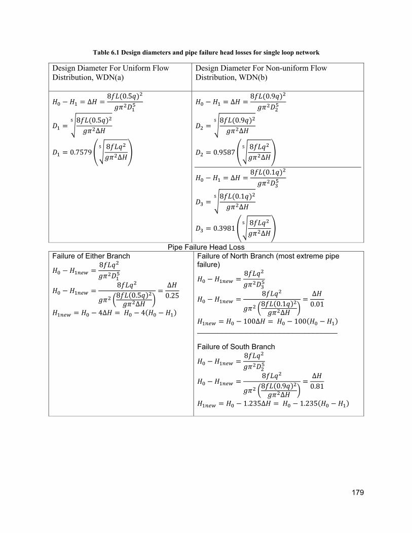
179

Table 6.1 Design diameters and pipe failure head losses for single loop network

Design Diameter For Uniform Flow Distribution, WDN(a)

Design Diameter For Non-uniform Flow Distribution, WDN(b)

𝐻 𝐻 ∆𝐻8𝑓𝐿 0.5𝑞

𝑔𝜋 𝐷

𝐷8𝑓𝐿 0.5𝑞

𝑔𝜋 ∆𝐻

𝐷 0.75798𝑓𝐿𝑞𝑔𝜋 ∆𝐻


𝑔𝜋 𝐷


𝑔𝜋 ∆𝐻



𝑔𝜋 𝐷


𝑔𝜋 ∆𝐻


Pipe Failure Head Loss Failure of Either Branch

𝐻 𝐻8𝑓𝐿𝑞

𝑔𝜋 𝐷


𝑔𝜋8𝑓𝐿 0.5𝑞

𝑔𝜋 ∆𝐻

∆𝐻0.25

𝐻 𝐻 4∆𝐻 𝐻 4 𝐻 𝐻

Failure of North Branch (most extreme pipe failure)


𝑔𝜋 𝐷



𝑔𝜋 ∆𝐻

∆𝐻0.01

𝐻 𝐻 100∆𝐻 𝐻 100 𝐻 𝐻 __________________________________ Failure of South Branch


𝑔𝜋 𝐷



𝑔𝜋 ∆𝐻

∆𝐻0.81

𝐻 𝐻 1.235∆𝐻 𝐻 1.235 𝐻 𝐻

180

Table 6.2 Cut-set analysis for Farhadgerd network with zero-meter pressure target, minimize-cost-maximize- Ir model

Cut‐Set Min

Cost, $ Max Cost,$

Mean Cost, $

Mean Ir

Mean Iu

Number of

Solutions

Mean Fraction

of Nodes Violated

30‐39 1.78E+07 1.80E+07 1.79E+07 0.021 0.078 3 0.116

40‐49 1.82E+07 3.43E+07 2.42E+07 0.060 0.030 554 0.081

50‐59 2.93E+07 5.16E+07 4.02E+07 0.066 0.010 443 0.046

60‐64 4.49E+07 5.16E+07 4.80E+07 0.066 0.008 89 0.024

181

Table 6.3 Cut-set analysis for Farhadgerd network with 20-meter pressure target, minimize-cost-maximize- Ir model

Cut‐Set Min

Cost, $ Max Cost,$

Mean Cost, $

Mean Ir

Mean Iu

Number of

Solutions

Mean Fraction

of Nodes Violated

0‐19 1.78E+07 2.02E+07 1.86E+07 0.034 0.067 5 0.165

20‐29 1.82E+07 2.05E+07 1.92E+07 0.045 0.036 21 0.132

30‐39 1.87E+07 2.55E+07 2.13E+07 0.057 0.036 264 0.109

40‐49 2.30E+07 4.64E+07 3.28E+07 0.065 0.016 564 0.072

50‐59 3.51E+07 5.16E+07 4.55E+07 0.066 0.008 136 0.037

60‐64 5.00E+07 7.21E+07 5.64E+07 0.066 0.010 10 0.024

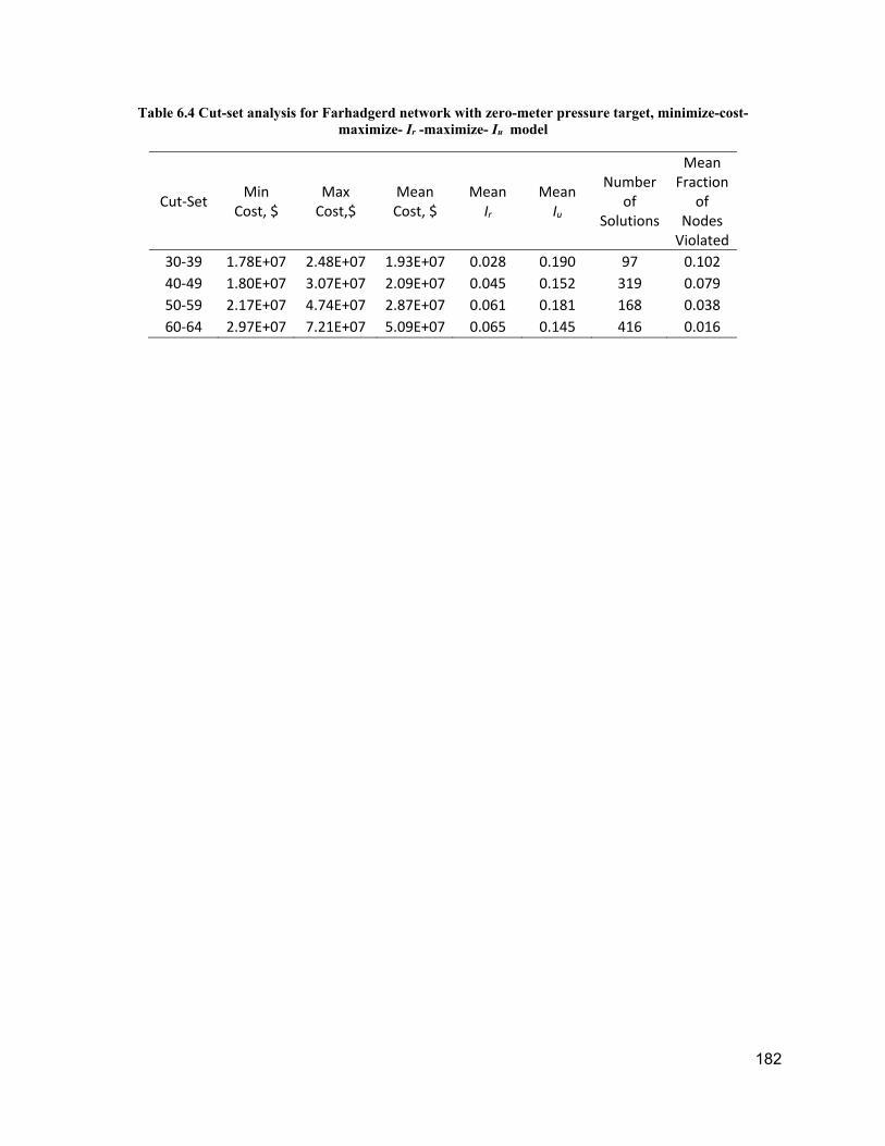
182

Table 6.4 Cut-set analysis for Farhadgerd network with zero-meter pressure target, minimize-cost-maximize- Ir -maximize- Iu model

Cut‐Set Min

Cost, $ Max Cost,$

Mean Cost, $

Mean Ir

Mean Iu

Number of

Solutions

Mean Fraction

of Nodes Violated

30‐39 1.78E+07 2.48E+07 1.93E+07 0.028 0.190 97 0.102

40‐49 1.80E+07 3.07E+07 2.09E+07 0.045 0.152 319 0.079

50‐59 2.17E+07 4.74E+07 2.87E+07 0.061 0.181 168 0.038

60‐64 2.97E+07 7.21E+07 5.09E+07 0.065 0.145 416 0.016

183

Table 6.5 Cut-set analysis for Farhadgerd network with 20-meter pressure target, minimize-cost-maximize- Ir -maximize- Iu model

Cut‐Set Min

Cost, $ Max Cost,$

Mean Cost, $

Mean Ir

Mean Iu

Number of

Solutions

Mean Fraction

of Nodes Violated

0‐19 1.78E+07 2.27E+07 1.95E+07 0.034 0.159 111 0.159

20‐29 1.78E+07 2.67E+07 2.01E+07 0.040 0.163 149 0.122

30‐39 1.81E+07 3.61E+07 2.19E+07 0.048 0.161 162 0.098

40‐49 2.18E+07 4.52E+07 2.75E+07 0.060 0.189 115 0.060

50‐59 2.32E+07 5.71E+07 3.61E+07 0.064 0.158 148 0.029

60‐64 3.00E+07 7.21E+07 5.49E+07 0.065 0.140 315 0.016

184

Table 6.6 Least cost designs for cut-set analysis accommodating 60-64 pipe removals for Farhadgerd network

Optimization Models

Min Cost Max Ir

0 m Target

Min Cost Max Ir, Iu 0 m Target

Min Cost Max Ir

20 m Target

Min Cost Max Ir, Iu

20 m Target

Cut‐set 60‐64 60‐64 60‐64 60‐64

Cost 4.49E+07 2.97E+07 5.00E+07 3.00E+07

Ir 0.066 0.064 0.066 0.064

Iu 0.004 0.109 0.009 0.123

Fraction of Nodes Violated

0.024 0.021 0.024 0.019

185

Table 6.7 Minimum pressure and location for a 10% increase in nodal demands for Farhadgerd network, least cost designs

Optimization Models

Min Cost Max Ir

0 m Target

Min Cost Max Ir, Iu 0 m Target

Min Cost Max Ir

20 m Target

Min Cost Max Ir, Iu

20 m Target

Cost 4.49E+07 2.97E+07 5.00E+07 3.00E+07

Min Pressure

22.6 22.1 22.6 22.1

Node Number

J‐41* J‐41 J‐41 J‐41

* J‐41 is located at downstream of pipe P‐48 (a branch pipe close to the reservoir)

186

(a)

(b)

Figure 6.1 Uniform flow single loop network, WDN(a), (b) Non-uniform flow single loop network, WDN(b)

187

Figure 6.2 Pareto-optimal frontier for Farhadgerd network

00.01

0.18

0.02

0.03

Uniformity Index

6 0.2

0.04

Cost

107

Res

ilien

ce In

dex

4

0.05

0.3

0.06

2

0.07

0.40($)

188

(a) minimize‐cost‐maximize‐Ir‐maximize‐Iu

model

(b) minimize‐cost‐maximize‐Ir

(c) both models Figure 6.3 Pareto-optimal frontier for Farhadgerd network considering cost and Ir, based on (a) minimize-

cost-maximize- Ir -maximize- Iu model, (b) minimize-cost-maximize- Ir , (c) both models

1 2 3 4 5 6 7 8

Cost ($) 107

0.01

0.02

0.03

0.04

0.05

0.06

0.07

Res

ilien

ce In

dex

Cost+Ir+Iu

1.5 2 2.5 3 3.5 4 4.5 5 5.5

Cost ($) 107

0.01

0.02

0.03

0.04

0.05

0.06

0.07

Re

silie

nce

Inde

x

Cost+Ir

1 2 3 4 5 6 7 8

Cost ($) 107

0.01

0.02

0.03

0.04

0.05

0.06

0.07

Res

ilien

ce In

dex

Two Objectives: Cost+IrThree Objectives: Cost+Ir+Iu

189

(a) pressure target zero‐meter, minimize‐

cost‐maximize‐Ir

(b) pressure target zero‐meter, minimize‐

cost‐maximize‐Ir‐maximize‐Iu

(c) pressure target 20‐meter, minimize‐

cost‐maximize‐Ir

(d) pressure target 20‐meter, minimize‐

cost‐maximize‐Ir‐maximize‐Iu Figure 6.4 Diameter distribution for Farhadgerd network, least cost solutions for the pipe cut-set with (a) Zero-meter pressure target, minimize-cost-maximize-Ir model, (b) Zero-meter pressure target, minimize-cost-maximize-Ir-maximize-Iu model, (c) 20-meter pressure target, minimize-cost-maximize-Ir model, (d) 20-meter pressure target, minimize-cost-maximize-Ir-maximize-Iu model

190

Chapter 7 : Approximation of Fuzzy Membership Functions in Water

Distribution Network Analysis

7.1 Preface

As shown in Figure 1.1, WDN analysis can be deterministic or non-deterministic. In deterministic

analysis, input parameters such as nodal demands, pipe characteristics and reservoir water levels

are assumed to be constant and certain and unknown variables such as pipe flows and nodal

pressures are evaluated. In response to those non-deterministic analysis, the aforementioned input

parameters do not have a certain value. In this case, Probability Theory identifies PDFs for

quantitative parameters and Fuzzy Set Theory identifies FM functions for linguistic parameters.

The unknown variables also may be reported as PDFs or FMs. There are several methods for non-

deterministic analysis such as MCS for incorporating both Probability and Fuzzy Set Theory,

FORM for incorporating Probability Theory, and Fuzzy Analysis techniques for incorporating

Fuzzy set theory. The main advantage of the application of Fuzzy Set Theory is the simple

construction of the FMs for uncertain linguistic variables. This technique can identify the extreme

values of unknown variables when uncertain input information ranges between pre-specified

extremes, and when the PDFs of the information cannot be obtained. There are two main

approaches for conducting the Fuzzy Analysis in WDN design: 1) 𝛼 level optimization and 2)

gradient-based methods. The 𝛼 level optimization technique is a very time-consuming process

which needs many hydraulic analyses for constructing MFs. The gradient-based method improves

the efficiency of the Fuzzy Analysis for middle-sized networks. However, this method is also not

readily applicable for large-sized networks. Approximations of the gradients of the equations that

govern WDN analysis, with respect to nodal demands and pipe resistance, are identified herein

and harnessed to accelerate Fuzzy Analysis of system hydraulics. The resulting WDN nodal

pressures are inversely proportional to nodal demands, and depending on flow directions,

proportional to pipe resistance.

7.2 Abstract

Design and analysis of water distribution networks (WDNs) is laden with uncertainty, both,

aleatory, i.e., natural randomness, such as variations in reservoir elevation heads, and epistemic,

i.e., incomplete knowledge, imprecise data, and linguistic ambiguity such as that associated with

characterization of pipe resistance, nodal demands, and hydraulic responses. To accommodate

191

aleatory uncertainty, stochastic analysis is applied to represent the input uncertainties and to

estimate resulting uncertainty in nodal pressures and pipe flows. In the analysis of WDNs facing

epistemic uncertainty, in particular, fuzzy set theory has widely been suggested as an alternative

to stochastic analysis. This technique can identify the extreme values of unknown variables when

uncertain input information ranges between pre-specified extremes, and when the probability

distribution of the information cannot be obtained. Current approaches for conducting fuzzy

analysis of WDNs to support operations and design are computationally demanding, and thus

limited in their applicability to large networks. Approximations of the gradients of equations that

govern WDN analysis, with respect to nodal demands and pipe resistance, are identified herein

and harnessed to accelerate fuzzy analysis of system hydraulics. The resulting WDN nodal

pressures are inversely proportional to nodal demands, and depending on flow directions,

proportional to pipe resistance. Results of fuzzy analyses for two realistically-sized WDNs show

that the proposed method performs with an acceptable level of accuracy and greatly reduces

computational time, relative to existing fuzzy analysis approaches.

7.3 Introduction

In practice, many model parameters for hydraulic analysis of water distribution networks (WDNs),

such as nodal demands and pipe roughness coefficients, are uncertain and therefore estimation of

crisp values for pressures and flows may not be realistic. If a parameter, such as water demand,

may be measured under differing system conditions, a probability density function of the

parameter may be estimated, and the resulting distribution of the simulation model output may be

obtained. When parameters cannot be measured directly, as is the case of pipe roughness

coefficients, such stochastic methods are not applicable. Revelli and Ridolfi (2002) introduce an

analysis of pipe networks that considers demands and pipe roughness coefficients as fuzzy

parameters and evaluates fuzzy pipe flows and nodal pressures resulting from these parameters.

A fuzzy parameter is represented by a fuzzy set, which defines the range of values for the

parameter, i.e., its support, its most-likely value, i.e., its kernel, and the degree of membership,

over the closed interval [0,1], at which the parameter is believed to range between any set of values.

Rather than apply hydraulic simulation directly, for each node, and a given degree of membership,

referred to as 𝛼, Revelli and Ridolfi (2002) employ an 𝛼 level optimization approach and

sequential quadratic programming (SQP) to approximate extreme values of the flow, and estimate

192

extreme values of the pressure based on these flows. For each node, the 𝛼 level optimization is

repeated for a range of 𝛼 levels from 0 to 1. Haghighi and Keramat (2012) employ this approach

with simulated annealing for estimating flows and pressures over time in transient hydraulic

analysis. Sivakumar et al. 2016 analyze four water distribution networks and estimate the

membership function of pipe discharges and hydraulic heads by assuming pipe roughness as

uncertain. All approaches employ triangular membership functions and are applied to small

networks.

Xu (2002) compares the fuzzy hydraulic model of Xu and Goulter (1999), which linearizes the

headloss equations, with the fuzzy hydraulic analysis of Revelli and Ridolfi (2002), and

demonstrates that, while the latter provides reliable estimates of uncertainty, its practical

application to larger networks is limited by its excessive computational requirements. Xu shows

that for a network with nn nodes and np pipes and for which nf degrees of membership are

considered, the approach of Revelli and Ridolfi (2002) would require solution of 2 𝑛𝑓 1

𝑛𝑛 1 nonlinear optimization models to characterize the uncertainty associated with nodal

pressure and pipe flow. He also asserts that for large networks, which may involve thousands of

nodes and pipes, the method of Revelli and Ridolfi (2002) may be less computationally efficient

than Monte Carlo Simulation. Furthermore, Gould et al. (2005) show that the SQP algorithm used

by Revelli and Ridolfi (2002) may only be efficient for small- and certain classes of large-scale

convex nonlinear problems.

In order to reduce the computational burden of fuzzy hydraulic analysis, Gupta and Bhave (2007)

propose a direct approach for estimating the extreme values of nodal pressures and pipe flows

which does not require iterative 𝛼 level optimization. Here, a hydraulic analysis is conducted

based on the most likely values of the pipe friction coefficients and nodal demands, and the

gradients of the hydraulic response at each node, to small changes in this input information, are

estimated with trial analyses. Assuming that the gradients of the hydraulic responses are constant

over the entire variable space, the extreme responses are then obtained by substituting the 𝛼 level

upper or lower bound of the input information in the hydraulic simulator. This approach requires

𝑛𝑓 1 3 𝑛𝑛 𝑛𝑝 1 hydraulic analyses, and is computationally demanding for large

networks. Spiliotis and Tsakiris (2012) apply the Newton-Raphson Method to estimate the

derivative of the coupled energy plus continuity equation, with respect to pressure and estimate

193

the fuzzy nodal pressures resulting from fuzzy demands and deterministic pipe roughness

coefficients. This approach requires solution of 𝑛𝑓 1 2 𝑛𝑛 1 nonlinear systems of

coupled energy plus continuity equations. Sabzkouhi and Haghighi (2016) apply an evolutionary

algorithm (particle swarm optimization) to solve an 𝛼 level optimization model for all nodal

pressures and pipe flows, simultaneously. In this case, the fuzzy parameters are demands, pipe

roughness coefficients, and reservoir water levels. For a small network (three nodes, five pipes,

and two loops) this approach requires 29,376 hydraulic simulations and for a network with 45

nodes, 65 pipes, and twenty loops, it requires 590,040 hydraulic simulations. Thus, this approach

is also computationally burdensome for the fuzzy analysis of large WDNs.

Fu and Kapelan (2011) argue that much of municipal design relies on imprecise and ambiguous

information and propose the use of fuzzy random variables to characterize such uncertainties in

WDN design. For each node in the WDN, they develop a fuzzy random variable that describes

the nodal pressures, and define the magnitude of failure of a given design as the fuzzy membership

at which this fuzzy variable is less than the fuzzy required pressures. For a given WDN design,

they use Monte Carlo sampling of the fuzzy nodal demands and pipe roughness coefficients to

estimate the extreme values of nodal pressures at each 𝛼 level. Thus, analysis of any WDN design

is computationally intensive as it requires the same number of hydraulic simulations as Monte

Carlo realizations. Dongre and Gupta (2017) formulate an optimization model for the least cost

design of WDNs and link the fuzzy hydraulic analysis of Gupta and Bhave (2007) to a genetic

algorithm to determine the optimal design. They apply the model to two benchmark networks and

demonstrate its effectiveness for improving design.

The approach developed in this paper improves fuzzy hydraulic analysis by reducing the

computational burden of finding the fuzzy membership functions of nodal pressures. First, the

analytical solution of the Co-Content Model (Bhave and Gupta 2006) is evaluated and the solution

is employed to approximate relationships between fuzzy nodal demands and/or pipe roughness

coefficients and fuzzy nodal pressures. The kernel of each fuzzy nodal demand and pipe roughness

coefficient is used to find the kernel of the fuzzy pressures at all nodes, using a hydraulic solver.

Given the flow directions for this solution, at each 𝛼 level, input values of fuzzy nodal demands

and pipe roughness coefficients are selected that will result in the extreme values of the fuzzy

nodal pressures as output to the hydraulic solver. In total, this approach requires 𝑛𝑓 1

194

2 𝑛𝑛 1 hydraulic analyses. In the following sections, the Co-Content Model, proposed

fuzzy analysis approach, and application of the approach to two realistically-sized WDNs is

presented. Results of these examples show that the proposed approach provides a close

approximation of the fuzzy uncertainty of nodal pressures and is computationally efficient.

7.4 Co-Content Model for WDN Analysis

In the Co-Content Model (Collins et al. 1978) the nodal pressures are considered unknown

variables and the coupled relationships for continuity at nodes and conservation of energy along

pipes are described with the following expressions.

Consider the energy loss due to friction in pipe k, 𝐸k, which is given by:

𝐸 𝑄 ℎ (7.1)

where 𝑄 is the flow at pipe k and ℎ is headloss in pipe k . For pipe k, which begins at node i

and ends at node j , ℎ is defined as:

ℎ 𝐻 𝐻 𝑅 𝑄 (7.2)

Where 𝐻 is the pressure at node i, 𝑅 is the characteristic pipe resistance coefficient which

depends on pipe roughness (e.g., Collins et al. (1978) defined it as a function of the Darcy-

Wiesbach friction factor (f) for pipe losses), length (L), and diameter (D), and n is the exponent of

the headloss equation and is specified for a given pipe type.

The unknown pipe flows may be expressed in terms of the nodal pressure and the known pipe

resistance as:

𝑄𝐻 𝐻

𝑅

(7.3)

Therefore, energy loss as a function of 𝐻 and R is expressed as:

𝐸𝐻 𝐻

𝑅

(7.4)

where 𝑅 is the headloss coefficient.

195

Bhave and Gupta (2006) reformulate the Co-Content Model as an unconstrained optimization that

minimizes total energy loss:

𝑀𝑖𝑛𝑖𝑚𝑖𝑧𝑒 𝐶𝐶𝐻 𝐻

𝑅

1𝑛

1 𝑞 𝐻

(7.5)

The first term of the objective function represents the energy loss within the pipes, and the second

term represents the energy loss due to withdrawals, where 𝑞 is the nodal flow demand. Flow

continuity at each node and energy conservation in each pipe are integral to the first term, and all

other energy losses are expressed in the second, thus the optimal solution of this objective satisfies

both nodal flow continuity and energy conservation relationships.

The matrix form of Co-Content Model is defined as:

𝑀𝑖𝑛𝑖𝑚𝑖𝑧𝑒 𝐶𝐶1

𝑅𝐴 𝑘, 𝑖 𝐻

1𝑛

1 𝑞 𝐻 (7.6)

where 𝐀 is an 𝑛𝑝 𝑛𝑛 incidence matrix that describes the topological relationships of the

network flows between nodes. Here, if a water source, or reservoir is located at a given node i,

the known elevation head of the source is used instead of 𝐻 . The elements of matrix 𝐀 are

defined as:

𝐴 𝑘, 𝑖1

01

𝑖𝑓 𝑡ℎ𝑒 𝑓𝑙𝑜𝑤 𝑜𝑓 𝑝𝑖𝑝𝑒 𝑘 𝑒𝑥𝑖𝑡𝑠 𝑛𝑜𝑑𝑒 𝑖

𝑖𝑓 𝑝𝑖𝑝𝑒 𝑘 𝑖𝑠 𝑛𝑜𝑡 𝑐𝑜𝑛𝑛𝑒𝑐𝑡𝑒𝑑 𝑡𝑜 𝑛𝑜𝑑𝑒 𝑖𝑖𝑓 𝑡ℎ𝑒 𝑓𝑙𝑜𝑤 𝑜𝑓 𝑝𝑖𝑝𝑒 𝑘 𝑒𝑛𝑡𝑒𝑟𝑠 𝑛𝑜𝑑𝑒 𝑖

(7.7)

7.5 Relationships for Demands, Pipe Resistance and Nodal Pressures

If the nodal demands and pipe resistance are known, the unknown 𝐻 may be estimated by

evaluating the derivative of CC with respect to 𝐻 and setting this equation equal to zero.

𝜕𝐶𝐶𝜕𝐻

1𝑛

11

𝑅𝐴 𝑘, 𝑖 𝐻 𝑞 0, ∀𝑖 1, … , 𝑛𝑛

(7.8)

By rearranging this equation an expression for the values of 𝑞 at optimality may also be

determined:

196

𝑞1

𝑅𝐴 𝑘, 𝑖 𝐻 , ∀𝑖 1, … , 𝑛𝑛

(7.9)

The relationship between nodal pressures and nodal demands may then be approximated, in order

to conduct a fuzzy analysis of pressure as a function of fuzzy demands, by evaluating the derivative

of the expression for 𝑞 (Eq. 7.9) with respect to 𝐻 :

𝜕𝑞𝜕𝐻

1𝑛

1

𝑅𝐴 𝑘, 𝑖 𝐻 , ∀𝑖 1, … , 𝑛𝑛

(7.10)

For a WDN operating under positive pressures, 𝜕𝑞 𝜕𝐻⁄ is always less than zero, and any variation

of 𝐻 is inversely proportional to any variation of 𝑞 . That is, as nodal demands increase, required

flows and corresponding friction losses increase, and resulting pressure heads decrease. Thus, the

maximum value of 𝐻 occurs at the minimum value of 𝑞 and the minimum value of 𝐻 occurs at

the maximum value of 𝑞 .

To find an approximation of the dependency of nodal pressures on pipe resistance, it is assumed

that variations of the pressure at a given node are only dependent on the resistance factors of pipes

which are connected to that node. Thus, Eq. (7.2) may be used to evaluate the derivative of the

expression for headloss with respect to 𝐻 and 𝐻 .

𝜕𝑅𝜕𝐻

0

𝜕𝑅𝜕𝐻

0

(7.11)

(7.12)

For a given pipe k, which lies between nodes i and j, an approximation of the variation of 𝑅 with

respect to changes in upstream pressure, 𝐻 , is positive and downstream pressure, 𝐻 , is negative.

Thus, for a given node, to find the maximum value of nodal pressure, resistance factors for all

pipes with flow directions entering the node should be set to their maximum values, and resistance

factors for all pipes with flow directions exiting the node should be set to their minimum values.

197

7.6 Fuzzy Analysis of WDNs

Given relationships between nodal demands, pipe resistance, and nodal pressures, the fuzzy

analysis of a WDN is undertaken as follows. First, the hydraulic simulation of the pipe network

is conducted using normal values (i.e., kernels of the fuzzy membership functions) of the nodal

demands and pipe resistance, and resulting pipe flows and directions are evaluated. Next, to find

the extreme values of pressures for each node, for a range of pre-defined 𝛼 levels, hydraulic

simulation of the network is undertaken using the appropriate 𝛼 level extreme values of the fuzzy

nodal demands and pipe resistance as input. To calculate the maximum value of pressure for a

given node i and 𝛼 level, 𝛼*, all nodal demands should be assigned their minimum input values at

the 𝛼* level:

𝐪 𝑞 ∗, ∀𝑗 1, … , 𝑛𝑛 (7.13)

and all pipe resistance values for pipes with flow entering the node should be assigned their

minimum values while all pipe resistance values for pipes with flow exiting the node should be

assigned their maximum values:

𝐑 �̅� 𝑖, 𝑘 ∗, ∀𝑘 1, … , 𝑛𝑝 (7.14)

where 𝐑 is the vector of resistance values for all pipes in the network, and �̅� 𝑖, 𝑘 is defined as:

�̅� 𝑖, 𝑘𝑅 ∗

𝑅 ∗

𝑖𝑓 𝑄 𝐴 𝑖, 𝑘 0𝑖𝑓 𝑄 𝐴 𝑖, 𝑘 0

(7.15)

where 𝑄 is obtained from hydraulic analysis of the network under normal conditions.

For calculation of the minimum value of the pressure for node i and 𝛼 level 𝛼*, all nodal demands

should be assigned their maximum input values at the 𝛼* level:

𝐪 𝑞 ∗, ∀𝑗 1, … , 𝑛𝑛 (7.16)

and all pipe resistance values for pipes with flow entering the node should be assigned their

maximum values while all pipe resistance values for pipes with flow exiting the node should be

assigned their minimum values:

𝐑 �̅� 𝑖, 𝑘 ∗, ∀𝑘 1, … , 𝑛𝑝 (7.17)

Where the matrix �̅� 𝑗, 𝑘 is defined as:

198

�̅� 𝑖, 𝑘 ∗𝑅 ∗

𝑅 ∗

𝑖𝑓 𝑄 𝐴 𝑖, 𝑘 0𝑖𝑓 𝑄 𝐴 𝑖, 𝑘 0

(7.18)

To obtain the complete membership functions of nodal pressures, this process is repeated for all

desired 𝛼 levels. While this analysis requires 𝑛𝑓 1 2 𝑛𝑛 1 simulations, if only nodal

demands are considered to be fuzzy, only 2𝑛𝑓 1 simulations are needed.

The performance of the method is evaluated herein for two example networks. In the first, a

medium-sized network, both demands at nodes and resistance factors in pipes are assumed to be

fuzzy and the method is compared with those of Gupta and Bhave (2007) and Revelli and Ridolfi

(2002), and in the second, a large-sized network, nodal demands are fuzzy and the method is

compared with that of Gupta and Bhave (2007) only, due to computational limitations. The

hydraulic simulations are conducted with the Global Gradient Algorithm (Todini and Pilati 1988),

and are executed in MATLAB with an Intel(R) Core(TM) 2Duo CPU P8700 @ 2.53 GHz and 4.00

GB RAM. Given the difference between the hydraulic analytic approach and the optimization

model of Revelli and Ridolfi, computational time is considered as a criteria for comparison of the

methods.

7.7 Examples

7.7.1 Nagpur Medium-Sized Network

Introduced by (Gupta and Bhave 2007), this network is based on that for the Gittikhadan Zone of

Nagpur, India. It has one source node, 179 pipes, 141 demand nodes, and 38 loops. A

representation of the network is shown in Figure 7.1. The source node is a reservoir with a surface

elevation of 335.84 m and supplies 755.26 l/s to the system. It is assumed that extreme values for

nodal demands are 𝑞 𝑞 – 𝜎𝑞 and 𝑞 𝑞 𝜎𝑞, and for the Darcy-Weisbach

coefficients of pipe roughness are 𝑓 𝑓 – 𝜎 𝑓, and 𝑓 𝑓 𝜎 𝑓, where q is the normal

nodal demand, f is the normal Darcy-Weisbach pipe roughness coefficient, and σ is the variability

which is set to 0.1. These assumptions and relevant network data, such as normal nodal demands,

pipe diameters, lengths, and connectivity are provided in Gupta and Bhave (2007).

Example resulting pressures for fifteen key nodes, using the proposed approach and those

developed by Revelli and Ridolfi (2002) and Gupta and Bhave (2007), are shown in Figure 7.2.

The nodal pressures based on the proposed method are nearly identical to those based on that of

199

Gupta and Bhave (2007). At the supports, the maximum pressure variation over all nodes for these

two approaches is almost three meters, but the maximum deviation between them is 6.57 cm. For

all nodes, the SQP algorithm in Revelli and Ridolfi (2002) does not converge to the global

optimum, and thus a suboptimal, narrower range, of nodal pressures are obtained. As summarized

in Table 7.1, this approach requires the solution of 1129 optimization models, taking

approximately 245 seconds per model to solve, and 76 hours in total to execute. The method of

Gupta and Bhave (2007) requires 2409 hydraulic simulations and 48.24 seconds in total, and the

proposed method requires 1129 hydraulic simulations and 22.64 seconds in total.

7.7.2 Hypothetical Large-Sized Network

This hypothetical network, introduced by Farmani et al. (2003), has 1892 nodes, 2467 pipes, and

two reservoirs. A representation of the network is shown in Figure 7.3. The range of normal nodal

demands are between zero and 0.1255 cms; and the range of resistance factors for pipes are set to

be between 0.0116 and 9.9952. Two cases are analyzed, where the extreme values for nodal

demands are 𝑞 𝑞 – 𝜎𝑞 and 𝑞 𝑞 𝜎𝑞, and the variability (σ) is 0.1 for the first case

, and 0.2 for the second. For both cases, the two methods converge to identical membership

functions for all nodes, and typical results are shown for nodes fourteen key nodes in Figure 7.4.

For the case with 10% variability, the maximum pressure variation for both methods at the support

is approximately 5% (i.e., nearly three meters), while for the case with 20% variability, it is

approximately 10% (i.e., nearly six meters). The method of Gupta and Bhave requires 22,705

hydraulic simulations and 31.5 hours in total. The proposed method requires 9 hydraulic

simulations and 45 seconds in total. Thus, for this large-sized network it may be readily used to

characterize the uncertainty in nodal pressures due to nodal demands, and, unlike other techniques,

is highly efficient, making it attractive for use in analysis of operations and design. While analysis

of the effect of uncertainty due to both demands and resistance would require on the order of 2000

hydraulic simulations per membership level, this would take on the order of 10,000 seconds only,

and thus considerably less effort than all existing methods.

7.8 Conclusion

While adoption of fuzzy set theory in hydraulic analysis has been gradual, its recent success in

advancing reliability-based design of all engineering systems portends its attractiveness for

simulating and optimizing WDNs. In the face of uncertainty, while probability theory is applicable

200

when the system inputs have unique distributions, fuzzy set theory accommodates imprecise,

incomplete, and ambiguous information in the design process, with an infinite number of possible

membership functions. Existing techniques for fuzzy pipe network analysis and design, such as

𝛼 level optimization, search methods for estimating the gradient of the hydraulic response, and

Monte Carlo Simulation, are limited in application to small networks due to their high

computational burden.

The fuzzy analytical approach introduced in this paper accelerates network analysis by

approximating the gradients of the reformulated Co-Content Model. Application of this method to

two example networks, which range in size and complexity, demonstrates its efficiency, accuracy,

and applicability. When only the nodal demands are fuzzy, this analysis requires only two network

simulations to find extreme pressures of all nodes. When both demands and pipe resistance are

fuzzy, two matrices are introduced based on the topological information of the network under

normal operating conditions, and these are used to find the extremes of the pressure boundaries.

Unlike other methods, where the computational effort, or the number of computationally

demanding optimization models to be solved, increases greatly with the size of the network, the

number of simulations of the approach presented herein increases only by two for each additional

node. This method results in comparable, and in some cases improved, accuracy, and exerts a

reduced computational burden in comparison with other methods. Its efficiency for large networks

allows for a broader analysis a range of possible scenarios for system conditions, stressors, and

hazards that plague these networks, many of which are unpredictable. Like all methods for

hydraulic analysis, it can also be used to assess the sensitivity of network operations to short- and

long-term changes in demands and proposed operational and structural improvements, and as a

means of measuring performance in optimal design of new systems.

201

Table 7.1 The comparison of different methods for Fuzzy analysis of the networks

Network Method CPU Time (s) Hydraulic Analysis

(EPANET Run)

Optimization of Nonlinear

Model Revelli and

Ridolfi 276605 - 1129

Nagpur Medium-Sized

Network

Bhave and Gupta

48.24 2409 -

Proposed Method

22.64 1129 -

Revelli and Ridolfi

N.A. N.A. N.A.

Hypothetical Large-Sized

Network

Bhave and Gupta

113400 22705 -

Proposed Method

45 9 -

202

Figure 7.1 Nagpur network

203

334.2 334.4 334.6 334.8 335 335.2

H1

0

0.2

0.4

0.6

0.8

1

332 332.5 333 333.5 334

H10

0

0.2

0.4

0.6

0.8

1

332.5 333 333.5 334 334.5

H20

0

0.2

0.4

0.6

0.8

1

332 332.5 333 333.5 334

H30

0

0.2

0.4

0.6

0.8

1

alp

ha-

leve

l

335 335.1 335.2 335.3 335.4 335.5

H50

0

0.2

0.4

0.6

0.8

1

alph

a-le

vel

331.5 332 332.5 333 333.5 334

H80

0

0.2

0.4

0.6

0.8

1al

pha-

leve

l

204

Figure 7.2 Fuzzy membership functions for H1, H10, H20, H30, H40, H50, H60, H70, H80, H90, H100, H110, H120, H130, and H140 obtained by the three fuzzy hydraulic analysis approaches

327 328 329 330 331 332

H110

0

0.2

0.4

0.6

0.8

1

alph

a-le

vel

205

Figure 7.3 EXNET network

206

45 50 55 60

H300

0

0.2

0.4

0.6

0.8

1

alph

a-le

vel

45 50 55 60

H600

0

0.2

0.4

0.6

0.8

1

alph

a-le

vel

48 50 52 54 56 58

H900

0

0.2

0.4

0.6

0.8

1al

pha-

leve

l

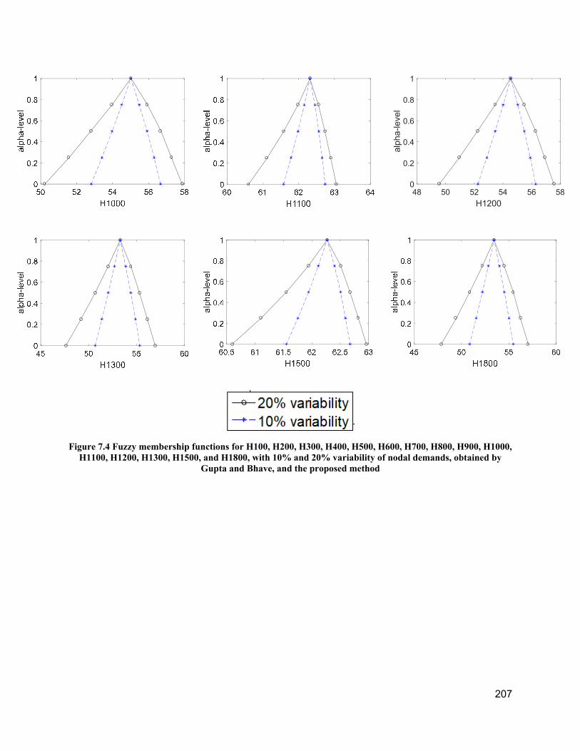
207

Figure 7.4 Fuzzy membership functions for H100, H200, H300, H400, H500, H600, H700, H800, H900, H1000, H1100, H1200, H1300, H1500, and H1800, with 10% and 20% variability of nodal demands, obtained by

Gupta and Bhave, and the proposed method

48 50 52 54 56 58

H1200

0

0.2

0.4

0.6

0.8

1

alph

a-le

vel

208

Chapter 8 : Conclusions

8.1 Summary of thesis objectives and methodologies

This thesis is organized based on the framework presented in Chapter 1, Figure 1.1. In this

framework, WDN modeling is classified into two efforts, WDN design and WDN analysis. WDN

design is classified as single- and multi-objective optimization models. WDN analysis is also

classified as deterministic or non-deterministic analysis. This thesis develops methods, algorithms,

and frameworks for enhancing these efforts. One of the main purposes of this thesis is to propose

efficient numerical methods for accelerating the design and/or analysis process for WDNs.

Another goal is to investigate different surrogates and propose methodologies for improvement of

the quality of WDN design. Research is conducted in three phases: 1) Chapters 2-4, investigate,

test, and develop different EAs for reducing the computational burden of both single- and multi-

objective WDN design; 2) Chapters 5 and 6, propose new frameworks and surrogates for

improvement of the design quality in the face of mechanical failures; and 3) Chapters 7, develops

numerical methods for acceleration of the Fuzzy analysis of WDNs. The research for each phase

began with an extensive literature review to select and synthesize key features of previous works,

evaluation approaches, and levels of detail. Then, fundamental equations of WDN modeling are

described, briefly. Next, the proposed methodologies are introduced and presented in detail.

Finally, several networks are used to demonstrate the efficiency of the proposed methodology in

comparison with popular works in the literature.

8.2 Research conducted

With reference to the research objectives and questions presented in Chapters 2-7, a summary of

the research conducted in this thesis is as follows:

8.2.1 Development of EAs for single- and multi-objective optimization of WDNs

Generally, the WDN optimization problem has an array of local optima which are, at times, very

different from each other. This characteristic is related to the need to satisfy minimum required

pressures at junctions throughout the network, and the required pressure is a nonlinear function of

the pipe size diameters and their configurations. By changing one pipe diameter, the flow direction

in the pipes, at least in the vicinity of the pipe, may change, and the distribution of the pressures

throughout the system may also change. This property makes the optimization of a network model

209

difficult to solve. Therefore, when the optimization algorithm is close to the global optimum, there

no guarantee that the optimum has been located, because the path for reaching the global optimum

may not necessarily be in the path taken near the best local optimum. EAs provide more diverse

solutions to escape from local optimum solutions effectively. They also exhibit independence from

the initial population of solutions, which, under classical optimization, determines the direction of

search. Finally, they do not concentrate solely on the evolution of the best solution (or solutions)

of the population.

The No-Free-Lunch (NFL) theorem asserts that no one optimization algorithm may be suited for

solving all kinds of optimization problems, and underscores the need for new algorithms that may

improve on efforts to reach global optima. Based on the NFL theorem and complexity of the pipe

network optimization problem, finding the best procedure for solving this problem is an open

question. Chapters 2-4, compare many popular EAs for single- and multi-objective optimization

of pipe networks and tests their performance using statistical analysis. By evaluating and

considering all benefits and demerits of different techniques, two modified versions of the DE

algorithm, FDE for single-objective and NSDE-RMO for multi-objective design, are proposed for

WDN design and are fast, reliable and have the least computational burden in comparison with

other optimization methods. The FDE algorithm is developed for both continuous- and discrete-

domain optimization problems and similar to the DE algorithm, it can solve nonlinear nonconvex

NP-hard problems. The high performance of its operators in comparison with other EAs in WDN

design and benchmark problems makes it an appropriate optimizer for other engineering

optimization problems.

8.2.2 Development of a new framework and introduction of new surrogates for improving

the quality of WDN design

In Chapter 5, a fuzzy multi-objective programming model for meeting competing objectives in the

optimal design of WDNs is proposed. Fuzzy membership functions for minimizing the pipe

network cost and maximizing a number of reliability surrogates are defined, and the model

maximizes the degree of satisfaction of these membership functions. Reliability surrogates

investigated include: i) the sum over all nodes of the relative surplus of energy at each node; ii)

the minimum surplus head at a critical node; iii) the sum over all nodes of the relative surplus of

energy at each node modified by the degree of pipe diameter uniformity of its associated loop; and

210

iv) the minimum pipe diameter uniformity of the associated loops over all nodes. An advantage

of this modeling framework is that it may be used to identify best compromise solutions that may

be investigated in greater detail. The benefits of this feature increase as the number of objectives

increase. Results demonstrate that the resilience index and its modifications, may be used as an

indirect measure of hydraulic reliability while they have some limitations in the face of mechanical

failures. In Chapter 6, a flow uniformity index is proposed to address these limitations and may be

considered a surrogate for mechanical reliability. The maximization of the uniformity index is

expected to lead to network designs with a balanced, increasingly uniform flow, at each node,

where the burden of carrying inflows (or outflows) at each node is shared evenly among all

incoming (or outgoing) pipes. The incorporation of the uniformity index, along with the goals of

maximizing the resilience index and minimizing design costs, in a multi-objective optimization

modelling framework results in WDN design solutions with increased mechanical reliability.

8.2.3 Advancement of numerical methods for Fuzzy Analysis of WDNs

Fuzzy Analysis of WDNs is a time consuming process which needs a large number of hydraulic

simulations to provide solutions. Chapter 7 shows how Fuzzy Analysis can effectively be applied

for evaluation of networks under uncertainty and also indicates that current methods, such as

𝛼 level optimization and MCS, are not efficient for generation of MFs for uncertain variables. In

this dissertation, a gradient-based method is proposed to approximate these MFs, which requires

the least amount of WDN simulations.

8.3 Suggestions for future work

Suggestions for future work are classified into four phases: 1) Application of efficient optimization

algorithms for multi-objective WDN design; 2) Applications of new surrogates in the reliability-

based optimization of WDNs; and 3) Development of a Fuzzy-Reliability approach for WDN

design under uncertainty.

8.3.1 Application of efficient optimization algorithms for multi-objective WDN design

As presented in the Chapters 2-4, modifications of classical DE for single-objective design, i.e.,

FDE, and for multi-objective design, i.e., NSDE-RMO, can significantly reduce the computational

burden of WDN optimization. Chapter 4 also demonstrates that FDE is an efficient algorithm for

finding a global optimum solution in the cost minimization of several networks. Therefore,

211

development of FDE for multi-objective models, considering cost and reliability surrogates is

necessary future research. For example, the accelerated mutation and crossover process of FDE

could be employed to identify the non-inferior set of solutions to a multi-objective problem. It may

be adapted to rank population members according to their objective function performance

crowding distance, and to use these ranks to modify the mutation operator and to sort in the

selection process.

Furthermore, in Chapter 5, the optimization process inside the Fuzzy programming model which

is currently conducted by the SLC algorithm, could be adapted to employ FDE. This application

of FDE may quickly converge to the global optimum and may indeed require fewer hydraulic

simulations with a reduced computational burden. A comparison among different multi-objective

EAs and the Fuzzy programming model also can be conducted.

8.3.2 Applications of new surrogates in reliability-based optimization of WDNs

Chapter 6 demonstrates that the uniformity index can improve the reliability of the network in the

face of mechanical failures. In this chapter, a multi-objective optimization model is employed for

minimizing cost and maximizing resilience and uniformity indices. In future work, these objectives

can be optimized in the Fuzzy programming model which converges to only one best compromise

design. Comparison of optimal solutions in population-based nondominated sorting and Fuzzy

programming models may reveal new characteristics of the uniformity index. Furthermore, other

variations of the uniformity index, such as the average of flow uniformity for all nodes, may

provide insightful information regarding design solutions. WDN optimization process can also be

conducted under uncertainty. In this case, instead of using a deterministic constraints for minimum

required pressures, failure probability can be approximated and implemented as an uncertain

constraint and may improve the design quality in real networks.

8.3.3 Development of Fuzzy-reliability concept for WDN design under uncertainty

Chapter 7 shows that Fuzzy Analysis is an appropriate application when Probability Theory and

Reliability analysis are not possible. However, the modification of Fuzzy analysis for WDN

design, i.e., for assessing Fuzzy failure rates for each design solution, is an open question. Here,

the main idea is to evaluate design solutions for networks under uncertainty to provide the degree

of reliability, or failure rate, when input parameters are fuzzy. Fuzzy indicators can be introduced

to describe the possible performance of design solutions. They may provide relative information

212

about the potential for, degree of, and ability to cope with failure, and may be incorporated in

multi-objective analysis to help decision makers select the best design(s), based on the available

budget and performance-based priorities. Fuzzy analysis of uncertainty may be instrumental in

achieving progress in several areas, most notably in the satisfaction of water quality targets

throughout the network, in the adaptation of an existing network to population growth and shifting

demands among user groups, and in the linked operation and design problems that plague water,

and in particular gas, supply networks. The generality of this approach may indicate promise for

its application in other engineering problems as well, such as in operation of networks of multi-

objective reservoirs, planning of transportation networks, and design of structures.

213

Bibliography

Ackley, D. H., (1987), “A Connectionist Machine for Genetic Hillclimbing”, Kluwer Academic

Publishers, Norwell, MA, USA.

Alperovitz, E., and Shamir, U. (1977), “Design of optimal water distribution systems”, Water

Resources Research, 13(6): 885–900.

Amirabdollahian, M., Asghari, K., and Chamani, M.R. (2011), “ Type 2 fuzzy logic system in

water network optimal design procedure”, 2011 International Conference on Information and

Intelligent Computing IPCSIT, 18 (2011) © (2011) IACSIT Press, Singapore.

Ang, W., and Jowitt, P. (2003), “Some observations on energy loss and network entropy in water

distribution networks”, Engineering Optimization, 35(4): 375-389.

Angira, R., and Babu, B. V., (2005), “Nondominated sorting differential evolution (NSDE): An

extension of differential evolution for multiobjective optimization”, Proceedings of the 2nd Indian

International Conference on Artificial Intelligence (IICAI-05), December 14-16, Pune, India,

1428–1443.

Atiquzzaman, M., Liong, S., and Yu, X. (2006). "Alternative decision making in water distribution

network with NSGA-II." ASCE Journal of Water Resources Planning and Management, 132(2):

122-126.

Atkinson, S., Farmani, R., Memon, F., and Butler, D. (2014), “Reliability indicators for water

distribution system design: comparison”, ASCE Journal of Water Resources Planning and

Management, 140(2): 160–168.

Babayan, A., Kapelan, Z., Savic, D., and Walters, G. (2005), “Least-cost design of water

distribution networks under demand uncertainty”, ASCE Journal of Water Resources Planning

and Management, 131(5): 375-382.

Babu, K. S. J., and Vijayalakshm, D.P., (2013), “Self-Adaptive PSO-GA hybrid model for

combinatorial water distribution network design”, Journal of Pipeline Systems Engineering and

Practice, ASCE, 4(1), 57-67.

Baños, R., Gil, C., Reca, J., and Ortega, J. (2010), “A Pareto-based memetic algorithm for

optimization of looped water distribution systems”, Engineering. Optimization, 42(3): 223-240.

214

Baños, R., Reca, J., Martínez, J., Gil, C., and Márquez, A.L. (2011), “Resilience indexes for water

distribution network design: A performance analysis under demand uncertainty”, Water Resources

Management, 25(10): 2351-2366.

Basupi, I., and Kapelan, Z. (2014), “Flexible water distribution system design under future

demand uncertainty”, ASCE Journal of Water Resources Planning and Management, 141(4): 1-

14.

Bhave, P. R., and Sonak, V. V., (1992), “A critical study of the linear programming gradient

method for optimal design of water supply networks”, Water Resources Research, 28(6): 1577-

1584.

Bhave, P.R., and Gupta, R. (2004), “Optimal design of water distribution networks for fuzzy

demands”, Civil Engineering and Environmental Systems, 21(4), 229-245.

Bhave, P. R., and Gupta, R. (2006), Analysis of Water Distribution Networks, Alpha Science

International, Technology & Engineering, the University of Michigan, 515 pages.

Bi, W., Dandy, G.C. and Maier, H.R., (2015), “Improved genetic algorithm optimization of water

distribution system design by incorporating domain knowledge”, Environmental Modelling &

Software, 69: 370–381.

Bolognesi, A., C. Bragalli, Marchi, A., and Artina, S., (2010), “Genetic heritage evolution by

stochastic transmission in the optimal design of water distribution networks”, Advances in

Engineering Software, 41(5): 792– 801.

Brest, J., Greiner, S., Boskovic, B., Mernik, M., and Zumer, V. (2006), “Self-adapting control

parameters in differential evolution: A comparative study on numerical benchmark problems”,

IEEE, Transactions on Evolutionary Computation, 10(6): 646–657.

Brooke, A., Kendrick, D., Meeraus, A., (1998), GAMS: a User’s Guide, The Scientific Press,

Redwood City, California, U.S.A, pp. 293.

Cail, Y., Zhao, M., Liao, J., Wang, T., Tian, H., and Chen, Y. (2017), “Neighborhood guided

differential evolution”, Soft Computing, 21(16):4769–4812.

Cisty, M, (2010), “Hybrid genetic algorithm and linear programming method for Least-Cost

Design of Water Distribution Systems”, Water Resources Management, 24(1): 1-24.

215

Chen, X., Wenli, D., and Feng Qian, F., (2014), “Multi-objective differential evolution with

ranking-based mutation operator and its application in chemical process optimization”,

Chemometrics and Intelligent Laboratory Systems, 136(15): 85–96.

Cohon, J. L. (1978), Multiobjective Programming and Planning. Academic Press, London.

Collins, M., Cooper, L., Helgason, R., Kenningston, J., and LeBlanc, L. (1978), “Solving the pipe

network analysis problem using optimization techniques” Management Science, 24(7): 747–760.

Creaco, E., Franchini, M., and Todini, E. (2016), “The combined use of resilience and loop

diameter uniformity as a good indirect measure of network reliability”, Urban Water Journal,

13(2): 167-181.

Creaco, E., Fortunato, A., Franchini, M., and Mazzola, M. R. (2014), “Comparison between

entropy and resilience as indirect measures of reliability in the framework of water distribution

network design”, Procedia Engineering, 70: 379–388.

Creaco, E., Franchini, M., and Todini, E. (2016), “Generalized resilience and failure indices for

use with pressure-driven modeling and leakage”, ASCE Journal of Water Resources Planning and

Management, 142(8): 1-10.

Cunha, M.C. and Sousa, J., (1999), “Water distribution network design optimization: simulated

annealing approach”, ASCE Journal of Water Resources Planning and Management, 125(4): 215–

221.

Cunha, M.C. and Sousa, J., (2001), “Hydraulic infrastructures design using Simulated Annealing”,

ASCE Journal of Infrastructure Systems, 7(1): 32–38.

Damelin, E., Shamir, U., and Arad N. (1972), “Engineering and economic evaluation of the

reliability of water supply”, Water Resources Research, 8(4): 861–877.

Dandy, G. C., Simpson, A. R., and Murphy, L. J. (1996), “An improved genetic algorithm for pipe

network optimization”, Water Resources Research, 32(2): 449–458.

Dandy, G. C., Wilkins, A., and Rohrlach, H., (2010), “A methodology for comparing evolutionary

algorithms for optimizing water distribution systems”, Proceedings of the 12th Water Distribution

System Analysis Symposium, September 12-15, Tucson, Arizona.

216

Das, S., Konar, A., and Chakraborty, U. K., (2005), “Two improved differential evolution schemes

for faster global search”, Proceedings of the ACM-SIGEVO GECCO, Washington, D.C., June

2005, 991–998.

Das, S., Abraham, A., Chakraborty, U. K., and Konar, A., (2009), “Differential evolution using a

neighborhood-based mutation operator”, IEEE Transactions on Evolutionary Computation,

13(3): 526 – 553.

Deb, K., Pratap, A., Agarwal, S., and Meyarivan, T. (2002), “A fast and elitist multiobjective

genetic algorithm: NSGA-II”, IEEE Transactions On Evolutionary Computation, 6(2): 182–197.

Di Nardo, A., Greco, R., Santonastaso, G. F., and Di Natale, M. (2010), “Resilience and entropy

indices for water supply network sectorization in district meter areas”, Proceedings of the

International Conference on Hydroinformatics, HIC 2010, Tianjin University, Tianjin, China,

2365–2373.

Dixon, L. C. W., and Szego, G. P., (1978), “The global optimization problem: an

introduction”, Towards Global Optimization, North-Holland Pub. Co, Amsterdam, 2: 1-15.

Dong, X., Liu, S., Tao, T., Li, S., and Xin, K., (2012), “A comparative study of differential

evolution and genetic algorithms for optimizing the design of water distribution systems”, Journal

of Zhejiang University SCIENCE A, 13(9): 674–686.

Duan, N., Mays, L.W., Lansey, K.E., (1990), “Optimal reliability based design of pumping and

distribution systems”, ASCE Journal of Hydraulic Engineering,116 (2): 249–268.

Egea, J.A., Martí, R., Banga, J.R. (2010), “An evolutionary method for complex-process

optimization”, Computers and Operations Research, 37 (2): 315-324.

Egea, J.A., Henriques, D., Cokelaer, T., Villaverde, A.F., MacNamara, A., Danciu, D.P., Banga,

J.R. and Saez-Rodriguez, J., (2014), “MEIGO: an open-source software suite based on

metaheuristics for global optimization in systems biology and bioinformatics”, BMC

Bioinformatics, 15(136): 1-9.

El-Ghandour1, H., and Emad Elbeltagi, E., (2018), “Comparison of five evolutionary algorithms

for optimization of water distribution networks”, ASCE Journal of Computing in Civil

Engineering, 32(1): 1-12.

217

Eusuff, M. M., and Lansey K. E. (2003), “Optimisation of water distribution network design using

Shuffled frog leaping algorithm”, ASCE Journal of Water Resources Planning and Management,

129(3): 210-225.

Farmani, R., Savic, D. A., and Walters, G. A. (2003), “Benchmark problems for design and

optimisation of water distribution systems”, In Proceedings of Advances in Water Supply

Management, Maksimovic, C., Butler, D., and Memon, F.A., eds., Balkema Publishers,

Rotterdam, The Netherlands, 249–256, June 2003.

Farmani, R., Savic, D. A., and Walters, G. A. (2005a), “Evolutionary multi-objective optimization

in water distribution network design”, Engineering Optimization, 37 (2): 167–183.

Farmani, R., Walters, G. A., and Savic, D. A. (2005b), “Trade-off between total cost and reliability

for Anytown water distribution network”, ASCE Journal of Water Resources Planning and

Management, 131(3): 161-171.

Farmani, R., Walters, G., and Savic, D. (2006), “Evolutionary multiobjective optimization of the

design and operation of water distribution network: total cost vs. reliability vs. water quality”,

Journal of Hydroinformatics, 8(3): 165–179.

Fonseca, C. M., and Fleming, P. J. (1993), “Genetic Algorithms for Multiobjective Optimization:

Formulation, Discussion and Generalization”, Proceedings of the Fifth International Conference

on Genetic Algorithms, 416–423, San Mateo, California. University of Illinois at Urbana-

Champaign, Morgan Kaufmann Publishers.

Friedman, M. (1937), “The use of ranks to avoid the assumption of normality implicit in the

analysis of variance”, Journal of the American Statistical Association, 32 (1937): 674–701.

Friedman, M. (1940), “A comparison of alternative tests of significance for the problem of m

rankings”, Annals of Mathematical Statistics, 11 (1940): 86–92.

Fu, G., and Kapelan, Z. (2011), “Fuzzy probabilistic design of water distribution networks”, Water

Resources Research, 47(5), 1-12, W05538.

Gamperle, R., Muller, S. D., and Koumoutsakos, A. (2002), “Parameter study for differential

evolution”, Proceedings of the WSEAS NNA-FSFS-EC 2002, Interlaken, Switzerland, 293–298.

218

Geem, Z.W., (2013), “Particle-swarm harmony search for water network design”, Engineering

Optimization, 41 (4): 297–311.

Geem, Z.W. (2006), “Optimal Cost Design of Water Distribution Networks Using Harmony

Search”, Engineering Optimization, 38(3): 259–280.

Geem, Z.W. (2015), “Multiobjective optimization of water distribution networks using fuzzy

theory and harmony search”, Water, 7: 3613-3625.

Giustolisi, O., Laucelli, D., and Colombo, A. (2009), “Deterministic versus stochastic design of

water distribution networks”, ASCE Journal of Water Resources Planning and Management,

135(2): 117-127.

Goldberg, D. E. (1983), Computer-aided Gas Pipeline Operation using Genetic Algorithms and

Rule Learning. Doctoral dissertation, University of Michigan, Ann Arbor, MI.

Gong, W., and Cai, Z. (2013), “Differential Evolution With Ranking-Based Mutation Operators”,

IEEE Transactions on Cybernetics, 43(6): 2066 – 2081.

Gould, N. I. M., Orban, D., and Toint, P. L. (2005), “Numerical methods for large-scale nonlinear

optimization”, Acta Numerica, Cambridge University Press, 2005, Printed in the United Kingdom,

299–361.

Goulter, I. C., and Bouchart, F. (1988), “Fuzzy programming in water distribution network

design”, in Proceedings of the 1st International Conference on Computer Methods and Water

Resources, 2, edited by D. Ouazar, C. A. Brebbia, and H. Barthet, 33–44, Comput. Mech. Publ.,

Southampton, Boston.

Greco, R., Di Nardo, A., and Santonastaso, G. (2012), “Resilience and entropy as indices of

robustness of water distribution networks”, Journal of Hydroinformatics, 14(3): 761–771.

Griewank, A. O. (1981), “Generalized Decent for Global Optimization”, Journal of Optimization

Theory and Applications, 34: 11–39.

Gupta, R., and Bhave, P. R. (2007), “Fuzzy parameters in pipe network analysis”, Civil

Engineering and Environmental Systems, 24(1): 33-54.

Haghighi, A., Samani, H. M V., and Samani, Z. M. V, (2011), “GA-ILP method for optimization

of water distribution networks”, Water Resources Research, 25: 1791–1808.

219

Hansen, N. and Kern, S., (2004), “Evaluating the CMA evolution strategy on multimodal test

functions”, In Eighth International Conference on Parallel Problem Solving from Nature PPSN

VIII, Proceedings, PPSN 2004. Lecture Notes in Computer Science, vol 3242. Springer, Berlin,

Heidelberg, 282-291.

Holger R. Maier, H.R., Simpson, A.R., Zecchin, A.C. and Foong, W.K. (2003), “Ant Colony

Optimization for Design of Water Distribution Systems”, ASCE Journal of Water Resources

Planning and Management, 129 (3): 200-209.

Holland, J. H. (1975), “Adaptation in Natural and Artificial Systems: An Introductory Analysis

with Applications to Biology”, Control, and Artificial Intelligence. Ann Arbor, MI: University of

Michigan Press, 1975.

Iorio, A. W., and Li., X. (2004), “Solving rotated multi-objective optimization problems using

differential evolution”, Proceedings of AI 2004: Advances in Artificial Intelligence, 3339: 861–

872.

Jaramillo, A., Crawford, B., Soto, R., Villablanca, S. M., Rubio, A. G., Salas, J., and Olguin, E.

(2016), “Solving the set covering problem with the Soccer League Competition algorithm”, Trends

in Applied Knowledge-Based Systems and Data Science, 9799: 884-891.

Jayaram, N., and K. Srinivasan (2008), “Performance-based optimal design and rehabilitation of

water distribution networks using life cycle costing”, Water Resources Research, 44, W01417,

doi:10.1029/2006WR005316.

Jeong, G., Wicaksono, A., and Kang, D. (2017), “Revisiting the resilience index for water

distribution networks”, ASCE Journal of Water Resources Planning and Management, 143(8): 1-

13.

Karaboga, D., (2005), An Idea Based on Honey Bee Swarm for Numerical Optimization, Technical

Report-TR06, Erciyes University, Engineering Faculty, Computer Engineering Department,

Kayseri/Türkiye.

Keedwell, E. and Khu, S.T., (2005), “Using cellular automata to seed genetic algorithms for water

distribution network design problems”, Engineering Applications of Artificial Intelligence, 18(4):

461-472.

220

Kennedy, J. and Eberhart, R.C. (1995), “Particle Swarm Optimization”, Proceedings of the 1995

IEEE International Conference on Neural Networks, 4: 1942–1948.

Kessler, A., Shamir, U., (1989), “Analysis of the linear programming gradient method for optimal

design of water supply networks”, Water Resources Research, 25 (7):1469–1480.

Kumar, P., (2017), Improved DE Algorithm with Information Utilization Selection for Constrained

Optimization, AIP Conference Proceedings, 1897(1), 10.1063/1.5008696, 19 October, India.

Lansey, K.E., Mays, L.W., (1989), “Optimization model for water distribution system design”,

ASCE Journal of Hydraulic Engineering, 115 (10): 1401–1418.

Lasdon, L.S., Waren, A., (1983), “GRG2: a user’s guide”, Department of General Business,

University of General Business, University of Texas, Austin, Texas.

Lence, B. J., Moosavian, N., and Daliri, H. (2017), “Fuzzy programming approach for

multiobjective optimization of water distribution systems”, ASCE Journal of Water Resources

Planning and Management, 143(7): 1-9.

Liang, C., Rong, W., and Dan, L. (2014), “An improved DE algorithm based on the New Crossover

Strategy”, Applied Mechanics and Materials, 713(715): 1583-1588.

Liebman, J.S., Lasdon, L., Scrage, L., Waren, A., (1986), “Modeling and Optimization with

GINO”, The Scientific Press, Palo Alto, California.

Lin, M.D., Liu, Y.H., Liu, G.F. and Chu, C.W. (2007), “Scatter Search Heuristic For Least-Cost

Design of Water Distribution Networks”, Engineering Optimization, 39 (7): 857–876.

Liong, S. Y., and Atiquzzaman, M., (2004), “Optimal design of water distribution network using

shuffled complex evolution”, Journal of The Institution of Engineers, 44 (1): 93–107.

Liu, H., Savić, D., Kapelan, Z., Zhao, M., Yuan, Y., and Zhao, H. (2014), “A diameter-sensitive

flow entropy method for reliability consideration in water distribution system design”, Water

Resources Research, 50: 5597–5610.

Liu, H., D. Savić, Z. Kapelan, M. Zhao, Y. Yuan, and H. Zhao (2014), “A diameter-sensitive flow

entropy method for reliability consideration in water distribution system design”, Water Resources

Research, 50: 5597–5610, doi:10.1002/2013WR014882.

221

Maier, H.R., Simpson, A.R., Zecchin, A.C., Foong, W.K., Phang, K.Y., Seah, H.Y. and Tan, C.L.

(2003), “Ant Colony Optimization For The Design of Water Distribution Systems”, Journal of

Water Resources Planning and Management, ASCE, 129 (3): 200–209.

Maier, H.R., Kapelan, Z., Kasprzyk, J., Kollat, J., Matott, L.S., Cunha, M.C., Dandy, G.C., Gibbs,

M.S., Keedwell, E., Marchi, A., Ostfeld, A., Savic, D., Solomatine, D.P., Vrugt, J.A., Zecchin,

A.C., Minsker, B.S., Barbour, E.J., Kuczera, G., Pasha, F., Castelletti, A., Giuliani, M., and Reed,

P.M. (2014), “Evolutionary algorithms and other metaheuristics in water resources: Current status,

research challenges and future directions”, Environmental Modelling & Software, 62(2014): 271-

299.

Marchi, A., Dandy, G., Wilkins, A., and Rohrlach, H. (2014), “Methodology for comparing

evolutionary algorithms for optimization of water distribution systems”, ASCE Journal of Water

Resources Planning and Management, 140(1): 22-31.

Martin, D.W., and Peters, G. (1963). “The application of Newton's method to network analysis

by digital computer.” Journal of Institution of Water Engineers and Scientists, 176(6): 115-129.

MATLAB [Computer software]. MathWorks, Natick, MA.

Maucec, M. S., Brest, J., Boskovic, B., Kacic, Z. (2018), “Improved Differential Evolution for

Large-Scale Black-Box Optimization”, Digital Object Identifier, 6: 29516 –29531, 10.1109/ IEEE

Access, 30 May.

Mays, L. W., and Cullinane, M. J. (1986), “A review and evaluation of reliability concepts for

design of water distribution systems”, Rep. M.P. EL-86-1, U.S. Army Eng. Waterways Exp. Stat.,

Vicksburg, Miss.

Mays, L. (1989), Reliability Analysis of Water Distribution Systems. American Society of Civil

Engineers, New York.

Min-Der L., Yu-Hsin Liu , Gee-Fon Liu and Chien-Wei Chu, (2007), “Scatter search heuristic for

least-cost design of water distribution networks”, Engineering Optimization, 39(7): 857-876.

Mininno, E., Neri, F., Cupertino, F., and Naso, D., (2011), “Compact Differential Evolution”,

IEEE Transactions on Evolutionary Computation, 15(1): 32-54.

222

Mirjalili, S. and Lewis, A. (2016), “The Whale Optimization Algorithm”, Advances in Engineering

Software, 95: 51-67.

Mirjalili, S., and Hashim, S. Z. M. 2010. A New Hybrid PSOGSA Algorithm for Function

Optimization, Computer and Information Application (ICCIA), 2010 International Conference on.

IEEE, 374-377.

Mladenović N, Hansen, P. (1997), “Variable neighborhood search”, Computers and Operations

Research, 24: 1097-1100.

Mohan, S., and Babu, K.S., (2010), “Optimal water distribution network design with honey-bee

mating optimization”, Journal of Computing in Civil Engineering, 24(1): 117-126.

Molga, M., and Smutnicki, C., (2013), “Test functions for optimization needs” (2005), Retrieved

June 2013, Available: http://www.zsd.ict.pwr.wroc.pl/files/docs/functions.pdf.

Montalvo, I., Izquierdo, J., Pérez, R., and Tung, M.M., (2008), “Particle swarm optimization

applied to the design of water supply systems”, Computers & Mathematics with Applications,

56(3): 769-776.

Moosavian, N and Roodsari, B.K. (2014), “Soccer League Competition Algorithm: A Novel Meta-

Heuristic Algorithm For Optimal Design of Water Distribution Networks”, Swarm and

Evolutionary Computation, 17: 14-24.

Moosavian, N., and Roodsari, B. K. (2014), “Soccer League Competition algorithm, a new method

for solving systems of nonlinear equations”, International Journal of Intelligence Science, 4(1): 7-

16.

Moosavian, N., and Jaefarzadeh, R. (2014), “Hydraulic analysis of water supply networks using a

Modified Hardy Cross method”, International Journal of Engineering, 27(9): 1331-1338.

Moosavian, N and Roodsari, B.K., (2014), “Soccer league competition algorithm: a novel meta-

heuristic algorithm for optimal design of water distribution networks”, Swarm and Evolutionary

Computation, 17: 14-24.

Moosavian, N. (2015), “Soccer league competition algorithm for solving knapsack problems”,

Swarm and Evolutionary Computation, 20: 14–22.

223

Moosavian, N., and Lence, B. (2016), “Nondominated Sorting Differential Algorithms for Multi-

Objective Optimization of Water Distribution Systems”, ASCE Journal of Water Resources


Moosavian, N., and Lence, B. (2017), “Testing Evolutionary Algorithms for Optimization of

Water Distribution Networks”, 23rd Canadian Hydrotechnical Conference (CSCE), (2017),

Vancouver, BC, Canada, 1-10.

Moosavian, N., and Lence, B. (2018), “Testing Evolutionary Algorithms for Optimization of

Water Distribution Networks”, Canadian Journal of Civil Engineering

(CSCE). https://doi.org/10.1139/cjce-2018-0137.

Moosavian, N. (2017), “Multilinear Method for Hydraulic Analysis of Pipe Networks”, ASCE

Journal of Irrigation and Drainage Engineering, 143(8): 1-12.

Murphy, L.J. and Simpson, A.R. (1992), “Pipe Optimization Using Genetic Algorithms”, Research

Rep. No. R93, Dept. of Civil Engineering, Univ. of Adelaide, Adelaide, Australia.

Murtagh, B.A., Saunders, M.A., (1992), “MINOS 5.1 User’s Guide”, Systems Optimization

Laboratory, Department of Operations Research, Stanford, California. Numerical Recipes,

Cambridge University Press, IInd ed.

Murphy, L.J. and Simpson, A.R., (1992), “Pipe Optimization Using Genetic Algorithms”,

Research Rep. No. R93, Dept. of Civil Engineering, Univ. of Adelaide, Adelaide, Australia.

Noman, N., and Iba, H. (2005), “Enhancing differential evolution performance with local search

for high dimensional function optimization”, Proceedings of the Genetic and Evolutionary

Computation Conference, GECCO 2005, Washington DC, USA, June 25-29, 967-974.

Omran, M., Salman, A., and Engelbrecht, A. P. (2005), “Self-adaptive differential evolution”,

International Conference on Computing Intelligence Security, Pt. 1, Springer Lecture Notes in

Artificial Intelligence 3801, 192–199.

Ostfeld, A., Oliker, N., and Salomons, E. (2014), “Multiobjective optimization for least cost

design and resiliency of water distribution systems”, Journal of Water Resources Planning and

Management, ASCE, 140(12): 1-12, 10.1061/(ASCE)WR.1943-5452.0000407, 04014037.

224

Peng, C., Sun, H., Guo, J., and Li, H., (2009), “A new algorithm based on nondominated sorting

differential evolution for multi-objective optimal load dispatch”, 2nd IEEE International

Conference on Computer Science and Information Technology, ICCSIT, 8-11 Aug, Beijing, 565–

569.

Perelman, L. and Ostfeld, A. (2007), “An Adaptive Heuristic Cross-Entropy Algorithm For

Optimal Design of Water Distribution Systems”, Engineering Optimization, 39 (4): 413–428.

Prasad, T. D., and Park, N. S. (2003), “Multiobjective genetic algorithms for design of water

distribution networks”, ASCE Journal of Water Resources Planning and Management, 130(1): 73-

82.

Prasad, T.D., Hong, S.H, and Park, N. (2003), “Reliability based design of water distribution

networks using multi-objective genetic algorithms”, KSCE Journal of Civil Engineering, 7(3):

351-361.

Prasad, T. and Park, N. (2004), “Multiobjective genetic algorithms for design of water distribution

networks”, Journal of Water Resources Planning and Management, ASCE,130(1): 73-82.

Prasad, T. D., and Tanyimboh, T. T. (2008), “Entropy based design of “Anytown” water

distribution network”, Proceedings, Water Distribution Systems Analysis 2008, J. E. Van Zyl, A.

A. Ilemobade, and H. E. Jacobs, eds., ASCE, Reston, VA, 450–461.

Price, K.V., Storn, R.M. and Lampinen, J.A. (2005), Differential Evolution: A Practical Approach

to Global Optimization, Springer Natural Computing Series, Berlin.

Quindry, G.E., Brill, E.D., Liebman, J.C., (1982), “Optimization of looped water distribution

systems”, Journal of Environmental Engineering Division, ASCE, 107(4): 665–679.

Raad, D. N. (2011), “Multi-Objective Optimization of Water Distribution Systems Design Using

Metaheuristics”, Univ. of Stellenbosch, Stellenbosch, South Africa.

Raad, D. N., Sinske, A. N., and Van Vuuren, J. H. (2010), “Comparison of four reliability surrogate

measures for water distribution systems design”, Water Resources Research, 46: W05524,

doi:10.1029/2009WR007785.

225

Raad, D., Sinske, A. and Van Vuuren, J. (2009), “Robust multi-objective optimization for water

distribution system design using a meta-metaheuristic”, International Transactions in Operational

Research, 16(5): 595–626.

Raad, D. N. (2011), “Multi-objective optimization of water distribution systems design using

metaheuristics”, University of Stellenbosch, Stellenbosch.

Rashedi, E., Nezamabadi, S., and Saryazdi, S. (2009), “GSA: A Gravitational Search Algorithm”,

Information Sciences, 179(13): 2232- 2248.

Rastrigin, L. A. (1974), Systems of extremal control, Nauka, Moscow (in Russian).

Reca, J., Martinez, J., Banos, R., and Gil, C. (2008), “Optimal design of gravity-fed looped water

distribution networks considering the resilience index”, ASCE Journal of Water Resources


Reca, J., and J. Martínez (2006), “Genetic algorithms for the design of looped irrigation water

distribution networks”, Water Resources Research, 42: W05416, doi: 10.1029/2005WR004383.

Reca, J., Martínez, J., and López, R., (2017), “A hybrid water distribution networks design

optimization method based on a search space reduction approach and a genetic algorithm”, Water,

9(2017): 1-11.

Revelli, R., and Ridolfi, L. (2002), “Fuzzy approach for analysis of pipe networks”, ASCE Journal

of Hydraulic Engineering, 128(1): 93–101.

Rosenbrock, H.H. (1960), “An automatic method for finding the greatest or least value of a

function”, The Computer Journal, 3 (3): 175–184.

Rossman, L. A. (2000). “EPANET 2 users manual.” Rep. No. EPA/600/ R-00/057, Water Supply

and Water Resources Division, National Risk Management Research Laboratory, Cincinnati.

Rozenberg, G., Bäck, T., and Eiben, A.E. (2005), “Differential evolution: A practical approach to

global optimization”, Springer, Berlin/Heidelberg, DEU. Available from: ProQuest ebrary.

Sabzkouhi, A. M., and Haghighi, A. (2016), “Uncertainty analysis of pipe-network hydraulics

using a many-objective particle swarm optimization”, ASCE Journal of Hydraulic Engineering,

142(9): 1-12.

226

Sadollah, A., Yoo D. G., and Kim J. H., (2014), “Improved mine blast algorithm for optimal cost

design of water distribution systems”, Engineering Optimization, 48(12): 2141-2156.

Saleh, S. H. A., and Tanyimboh, T. T. (2014), “Optimal design of water distribution systems based

on entropy and topology”, Water Resources Management, 28(11): 3555-3575.

Savic, D. A., and Walters, G. A. (1997), “Genetic algorithms for least cost design of water

distribution networks”, Journal of Water Resources Planning and Management, ASCE, 123(2):

67-77.

Schaake, J.C., and Lai, D., (1969), “Linear programming and dynamic programming applications

to water distribution network design”, Rep. 116, Hydrodyn. Lab., Mass. Inst. Of Technol.,

Cambridge, Mass.

Schwartz, R., Housh, M., and Ostfeld, A. (2016), “Limited multistage stochastic programming for

water distribution systems optimal operation”, Journal of Water Resources Planning and

Management, ASCE, 142(10): 1-6, 06016003.

Schwefel, H.P., (1981), Numerical Optimization of Computer Models, John Wiley & Sons,

Chichester, UK.

Sedki, D. Ouazar, (2012), “Hybrid particle swarm optimization and differential evolution for

optimal design of water distribution systems”, Advanced Engineering Informatics, 26 (3): 582–

591.

Shamir, U., and Howard, C. D. D. (1981), “Water supply reliability theory”, Journal of the

American Water Works Association, 73(7): 379-384.

Sheikholeslami, R., and Zecchin, A.C., Zheng, F., and Talatahari, S., (2016), “A hybrid cuckoo-

harmony search algorithm for optimal design of water distribution systems”, Journal of

Hydroinformatics, 18(3): 544-563.

Simpson, A. R., Dandy, G. C., and Murphy, L.J., (1994), “Genetic algorithms compared to other

techniques for pipe optimization”, Journal of Water Resources Planning and Management, ASCE,

120(4): 423–443.

Spiliotis, M., and Tsakiris, G. (2012), “Water distribution network analysis under fuzzy demands”,

Civil Engineering and Environmental Systems, 29(2): 107-122,

227

Srinivas N., and Deb, K. (1994), “Multiobjective optimization using nondominated sorting in

genetic algorithms”, Evolutionary Computation, 2(3): 221–248.

Storn, R., and Price, K. (1997), “Differential evolution - a simple and efficient heuristic for global

optimization over continuous spaces”, Journal of Global Optimization, 11(4): 341-359.

Suribabu, C. R. and Neelakantan, T. R., (2006a), “Particle swarm optimization compared to other

heuristic search techniques for pipe sizing”, Journal of Environmental Informatics, 8 (1): 1–9.

Suribabu, C.R., and Neelakantan, T. R., (2006b), “Design of water distribution networks using

particle swarm optimization”, Urban Water Journal, 3(2): 111-120.

Suribabu, C. R. (2010), “Differential evolution algorithm for optimal design of water distribution

networks”, Journal of Hydroinformatics, 12(1): 66-82.

Teo, J. (2006), “Exploring dynamic self-adaptive populations in differential evolution”, Soft

Computing–Fusion Foundation, Methodologies Applicat., 10(8): 673–686.

Todini E., and Pilati S. (1988), “A gradient method for the solution of looped pipe networks”,

International Conference on Computer Application for Water Supply and Distribution. Leicester

Polytechnic, UK, Wiley, London, 1–20.

Todini, E. (2000), “Looped water distribution networks design using a resilience index based

heuristic approach”, Urban Water Journal, 2(2): 115-122.

Todini E. (2006), “On the convergence properties of the different pipe network algorithms”, 8th

Annual Water Distribution Systems Analysis Symposium, Cincinnati, Ohio, USA.

Todini, E., and Rossman, L. (2013), “Unified Framework for Deriving Simultaneous Equation

Algorithms for Water Distribution Networks”, Journal of Hydraulic Engineering, 139(5): 511 –

526.

Tolson, B. A., Asadzadeh, M., Maier, H. R., and Zecchin, A. (2009), “Hybrid discrete dynamically

dimensioned search (HD-DDS) algorithm for water distribution system design optimization”,

Water Resources Research, 45: W12416, doi: 10.1029/2008WR007673.

Tolson, B. A., Maier, H. R., Simpson, A. R., and Lence, B. J. (2004), “Genetic algorithms for

reliability-based optimization of water distribution systems”, ASCE Journal of Water Resources

Planning and Management, 130(1): 63–72.

228

Tolson, B. A., M. Asadzadeh, H. R. Maier, and A. Zecchin, (2009), “Hybrid discrete dynamically

dimensioned search (HD-DDS) algorithm for water distribution system design

optimization”, Water Resources Research, 45, W12416, doi:10.1029/2008WR007673.

Torn A. and Zilinskas, A., (1980), “Global Optimization”, Lecture Notes in Computer Science No.

350, Springer Verlag, Berlin.

Vamvakeridou, L. S., Savic, D.A., and Walters, G.A. (2006), “Fuzzy hierarchical decision support

system for water distribution network optimization”, Civil Engineering and Environmental

Systems, 23(3): 237-261. Vasan, A. and Simonovic, S. (2010), “Optimization of Water Distribution Network Design Using

Differential Evolution”, Journal of Water Resources Planning and Management, ASCE, 136 (2):

279–287.

Vrugt, J. A., and Robinson, B. A. (2007), “Improved evolutionary optimization from genetically

adaptive multimethod search,” Proceedings of the National 1212 Academy of Sciences of the

United States of America, 104: 708-711.

Vrugt, J. A. (2015), “Multi-criteria Optimization Using the AMALGAM Software Package:

Theory, Concepts, and MATLAB Implementation”, Manual Version 1.0, 53 pp.

Wang, Q., Guidolin, M., Savic, D., and Kapelan, Z. (2014), “Two-objective design of benchmark

problems of a water distribution system via MOEAs: towards the best-known approximation of

the true Pareto front”, Journal of Water Resources Planning and Management, ASCE, 141(3): 1-

14, 04014060.

Wolpert, D.H. and Marcready W.G. (1997), “No Free Lunch Theorems For Optimization”, IEEE

Transactions On Evolutionary Computation, 1(1): 67-82.

Wood D.J., and Charles C.O.A. (1972). “Hydraulic network analysis using linear theory.” Journal

of the Hydraulics Division, ASCE, 98(7), 1157-1170.

Wood D.J., and Charles C.O.A. (1973). “closure to discussions to Wood and Charles (1972):

Hydraulic network analysis using linear theory.” Journal of the Hydraulics Division, ASCE,

99(11), 21-29.

229

Wood, D. J. (1980). User's Manual-Computer Analysis of Flow in Pipe Networks including

Extended Period Simulations, University of Kentucky, Lexington, Ky.

Wood D.J., and Funk, J.E. (1993). “Hydraulic analysis of water distribution systems”, Proceedings

of the International Conference on Water Supply Systems State of the Art and Future. Trends,

Valencia, Spain, Oct. 1992, Computational Mechanics Publications, 43, 85.

Xu, T. Y., and Qin, X. S. (2013), “Applying an extended fuzzy parametric approach to the problem

of water allocations”, Mathematical Problems in Engineering, 2013, Article ID 647569, 10 pages,

2013. doi:10.1155/2013/647569.

Xu, C. and Goulter, I. C. (1999), “Optimal design of water distribution networks using fuzzy

optimization”, Civil Engineering and Environmental Systems, 16(4): 243-266.

Xu C. (2002), “Discussion of Fuzzy approach for analysis of pipe networks, by Revelli, R., and

Ridolfi, L.”, ASCE Journal of the Hydraulic Engineering, 128(1): 93-101.

Yang, Z., He, J., and Yao, X., (2007), “Making a difference to differential evolution,” Advances

in Metaheuristics for Hard Optimization, Natural Computing Series. Springer, Berlin, Heidelberg,

415–432.

Yu, (1973), “A class of decisions for group decision problems”, Management Science, 19(8): 936-

946.

Zadeh, L. A. (1965), “Fuzzy sets”, Information and Control, 8 (3): 338–353.

Zeleny, M. (1974a), Linear Multi-objective Programming. Springer-Varlag, New York.

Zeleny, M. (1974b), “A concept of compromise solutions and the method of the displaced ideal”,

Computers and Operations Research, 1: 479-496.

Zecchin, A.C., Maier, H.R., Simpson, A.R., Leonard, M., Roberts, A.J., and Berrisford, M.J.,

(2006), “Application of two ant colony optimization algorithms to water distribution system

optimization”, Mathematical and Computer Modelling, 44: 451–468.

Zecchin, A., Thum, P., Simpson, A., and Tischendorf, C. (2012), “Steady-state behavior of large

water distribution systems: algebraic multigrid method for the fast solution of the linear

step”, Journal of Water Resources Planning and Management, ASCE,138(6): 639-650.

230

Zhao, Y., and Liu, J., (2014), “An improved differential evolution algorithm for practical dynamic

scheduling in steelmaking-continuous casting production Lixin Tang”, IEEE, Transactions on

Evolutionary Computation, 18(2): 209-225.

Zheng, F., A. R. Simpson, and A. C. Zecchin, (2011), “A combined NLP-differential evolution

algorithm approach for the optimization of looped water distribution systems”, Water Resources

Research, 47: W08531.

Zheng, F., Zecchin, A.C. and Simpson, A.R. (2013), “Self-Adaptive Differential Evolution

Algorithm Applied to Water Distribution System Optimization”, Journal of Computing in Civil

Engineering, ASCE, 27(2): 148–158.

Zheng, F., Simpson, A.R. and Zecchin, A.C., (2014), “Coupled binary linear programming–

differential evolution algorithm approach for water distribution system optimization”, Journal of

Water Resources Planning and Management, ASCE, 140(5): 585-597.

Zimmermann, H.J. (1991). Fuzzy Set Theory and Its Applications. Revised edition. Kluwer

Academic Publishers, Boston/Dordrecht/London.

Zitzler, E., and Thiele, L. (1999), “Multiobjective evolutionary algorithms: a comparative case

study and the Strength Pareto Approach”, IEEE Transactions on Evolutionary Computation, 3(4):

257–271.

Zitzler, E., Thiele, L., Laumanns, M., Fonseca, C. M., and da Fonseca, V. G. (2003), “Performance

assessment of multiobjective optimizers: An analysis and review”, IEEE Transactions on

Evolutionary Computation, 7(2): 117–132.

231

Appendices

Appendix A. The FDE code for minimization of the Sphere Function in Python

import numpy Maxit=1000 # number of iteration nPop=100 # number of population NumVariable=10 # number of decision variable Varmin=-100*numpy.ones(NumVariable) Varmax=100*numpy.ones(NumVariable) def Costfunction(x): a0= numpy.array(x) y0 = sum(a0*a0) # Sphere function return y0 class BestSol: def __init__(self,Cost,Position,Trial): BestSol.Cost=Cost BestSol.Position=Position BestSol.Trial=Trial Beta=0.5 # Mutation rate Pcr=0.4 # Crossover rate nEval=0 BestSol.Cost=10e10 FCost=10e10 a=numpy.zeros((nPop,NumVariable)) f=numpy.zeros(nPop) trial=numpy.zeros(nPop) # Counter inum=numpy.zeros(nPop) # Create inital population for i in range (0,nPop): a[i,:] = numpy.random.uniform(Varmin,Varmax,NumVariable) f[i]=Costfunction(a[i,:]) trial[i]=0 nEval=nEval+1 if f[i]<BestSol.Cost: BestSol.Position=a[i,:] BestSol.Cost=f[i] BestSol.Trial=trial[i] nPop1=nPop # Start FDE for it in range (0,Maxit): k=0 for i in range (0,nPop): if trial[i] > 30: inum[k]=i k=k+1 if k>0 and nPop>0.1*nPop1:

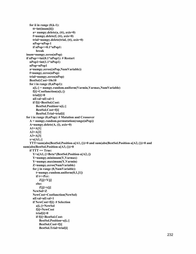
232

for ii in range (0,k-1): tt=int(inum[ii]) a= numpy.delete(a, (tt), axis=0) f=numpy.delete(f, (tt), axis=0) trial=numpy.delete(trial, (tt), axis=0) nPop=nPop-1 if nPop<=0.1*nPop1: break inum=numpy.zeros(nPop) if nPop<=int(0.1*nPop1): # Restart nPop1=int(1.1*nPop1) nPop=nPop1 a=numpy.zeros((nPop,NumVariable)) f=numpy.zeros(nPop) trial=numpy.zeros(nPop) BestSol.Cost=10e10 for i in range (0,nPop1): a[i,:] = numpy.random.uniform(Varmin,Varmax,NumVariable) f[i]=Costfunction(a[i,:]) trial[i]=0 nEval=nEval+1 if f[i]<BestSol.Cost: BestSol.Position=a[i,:] BestSol.Cost=f[i] BestSol.Trial=trial[i] for i in range (0,nPop): # Mutation and Crossover A = numpy.random.permutation(range(nPop)) A=numpy.delete(A, (i), axis=0) A1=A[1] A2=A[2] A3=A[3] x=a[A1,:] TTT=sum(abs(BestSol.Position-a[A1,:]))>0 and sum(abs(BestSol.Position-a[A2,:]))>0 and sum(abs(BestSol.Position-a[A3,:]))>0 if TTT == True: Y=a[A1,:]+Beta*(BestSol.Position-a[A2,:]) Y=numpy.minimum(Y,Varmax) Y=numpy.maximum(Y,Varmin) Z=numpy.zeros(NumVariable) for j in range (0,NumVariable): t=numpy.random.uniform(0,1,[1]) if t<=Pcr: Z[j]=Y[j] else: Z[j]=x[j] NewSol=Z NewCost=Costfunction(NewSol) nEval=nEval+1 if NewCost<f[i]: # Selection a[i,:]=NewSol f[i]=NewCost trial[i]=0 if f[i]<BestSol.Cost: BestSol.Position=a[i,:] BestSol.Cost=f[i] BestSol.Trial=trial[i]

233

else: BestSol.Trial=BestSol.Trial+1 else: trial[i]=trial[i]+1 if BestSol.Cost<FCost: FCost=BestSol.Cost print('iteration',it,'Cost Function',FCost,)

Appendix B Pipe and nodal information for Farhadgerd network

Table B.1 Candidate pipe size diameters and corresponding costs

($/meter length) for Farhadgerd network

Diameter (mm)


63.8 638 79.2 792 96.8 968 150 1500 200 2000 250 2500 300 3000 350 3500 400 4000

234

Table B.2 Nodal information for Farhadgerd network

Node Elevation

(m) Demand (L/s) Node

Elevation (m)

Demand (L/s)

R-1 510 - J-28 454.5 0.9242 J-1 479 2.1037 J-29 458 1.0336 J-2 468.7 3.3318 J-30 455.8 1.2403 J-3 466.5 1.4227 J-31 437 1.4462 J-4 467.1 0.5594 J-32 434.6 0.9990 J-5 469 0.1581 J-33 430 1.3035 J-6 467.3 1.2282 J-34 439.4 0.3996 J-7 469.2 2.4685 J-35 433.3 16.3083 J-8 460.5 0.3891 J-36 437 1.1037 J-9 461.3 4.5357 J-37 455.6 0.5594

J-10 465.4 0.9850 J-38 468.5 10.3238 J-11 476.3 0.4621 J-39 472.7 0.9850 J-12 477 0.6931 J-40 478.7 0.9485 J-14 472.5 0.1581 J-41 486 0.9971 J-15 478.7 0.6688 J-42 477.5 0.3770 J-16 478.5 0.5594 J-43 473.3 0.7053 J-17 475.5 4.7546 J-44 471.4 2.1037 J-18 475 0.2067 J-49 431.2 0.3140 J-19 480 0.3162 J-50 431.8 0.1618 J-20 472 1.3133 J-51 462.8 3.5872 J-21 456.2 0.6931 J-52 440 0.0000 J-22 458.3 1.2890 J-53 454.5 0.1000 J-23 446.3 0.8147 J-13 455.8 0.0000 J-24 440 0.5715 J-45 455.8 0.0000 J-25 445.4 1.5200 J-47 440 0.0000 J-26 438 2.7688 J-48 440 0.0000 J-27 441 2.0076 J-46 455.8 0.0000

235

Table B.3 Pipes characteristics for Farhadgerd network

Node J-in J-out L (m) C Node J-in J-out L (m) Hazen-

Williams factor, C

P-1 R-1 J-1 885.3851 120 P-41 J-35 J-36 437.3994 130 P-2 J-1 J-2 328.5421 120 P-42 J-36 J-26 359.4174 130 P-3 J-2 J-3 86.0021 120 P-43 J-30 J-37 141.5928 130 P-4 J-3 J-4 195.1899 120 P-44 J-37 J-38 667.3086 130 P-5 J-4 J-5 30.9500 120 P-45 J-38 J-39 242.5379 120 P-6 J-5 J-6 68.4875 130 P-46 J-39 J-40 229.1806 130 P-7 J-6 J-7 563.0813 130 P-48 J-41 J-42 203.4631 130 P-8 J-7 J-8 417.1908 130 P-49 J-42 J-43 100.3686 130 P-9 J-8 J-9 416.8621 120 P-50 J-43 J-29 503.9709 120

P-10 J-9 J-4 294.4953 120 P-51 J-38 J-44 385.2943 130 P-11 J-7 J-10 367.3761 130 P-57 J-32 J-49 190.6523 130 P-12 J-10 J-11 372.3605 130 P-58 J-49 J-50 208.6375 130 P-13 J-11 J-12 147.7453 130 P-59 J-50 J-33 227.8588 130 P-16 J-14 J-15 213.1492 130 P-60 J-34 J-31 278.1212 120 P-17 J-15 J-16 233.7499 130 P-61 J-7 J-14 322.7427 130 P-18 J-14 J-17 315.1370 130 P-62 J-12 J-16 193.8307 130 P-19 J-17 J-18 247.3020 130 P-63 J-27 J-35 354.9940 130 P-20 J-18 J-19 155.8379 130 P-64 J-2 J-51 342.1014 130 P-21 J-19 J-20 138.7134 130 P-56 J-51 J-28 299.1446 130 P-22 J-20 J-5 302.7770 130 P-55 J-1 J-43 135.5139 120 P-23 J-9 J-21 202.5051 130 P-54 J-43 J-39 444.0197 120 P-25 J-22 J-3 421.6994 130 P-53 J-45 J-31 505.6546 120 P-26 J-21 J-23 451.5464 130 P-52 J-47 J-26 247.9111 130 P-27 J-23 J-24 94.9841 130.013 P-47 J-53 J-27 445.0974 130 P-28 J-24 J-25 138.8879 130 P-38 J-52 J-53 504.6454 130 P-29 J-25 J-22 381.8934 130.013 P-36 J-53 J-13 468.0775 130 P-33 J-28 J-25 388.1121 130 P-32 J-48 J-52 16.5572 130 P-34 J-28 J-29 348.5208 130 P-31 J-46 J-13 16.3047 120 P-35 J-29 J-30 125.7833 120 P-30 J-45 J-13 52.5861 120 P-37 J-31 J-32 333.0668 130 P-24 J-46 J-30 14.3932 120 P-39 J-33 J-34 286.3284 130 P-15 J-47 J-52 74.3145 130 P-40 J-34 J-35 436.9019 130 P-14 J-48 J-24 13.5482 130 P-65 J-46 J-30 14.3932 120 P-66 J-46 J-13 16.3047 120 P-67 J-48 J-24 13.5482 130 P-68 J-48 J-52 16.5572 130

236

Documents

Optimal Design of Water Distribution Networks under