OPTIMAL DESIGN OF IRRIGATION NETWORKS USING THE …OPTIMAL DESIGN OF IRRIGATION NETWORKS USING THE DYNAMIC METHOD AND A SIMPLIFIED NONLINEAR METHOD ... in the management of the water

OPTIMAL DESIGN OF IRRIGATION NETWORKS USING THE DYNAMIC METHOD AND A SIMPLIFIED NONLINEAR METHOD

M. THEOCHARIS1 , C. TZIMOPOULOS 2 , S. YANNOPOULOS 2 AND M. SAKELLARIOU - MAKRANTONAKI 3

1 Department οf Crop Production Technical Educational Institution of Epirus

47100 Arta, GREECE http://www.teiep.gr

2 Department of Rural and Surveying Engineers Aristotle University of Thessaloniki

54006 Thessaloniki, GREECE 3 Department of Agricultural Crop Production and Rural Environment

University of Thessaly 38334 Volos, GREECE

Abstract: - The designating factors in the design of branched irrigation networks are the cost of pipes and the cost of pumping. They both depend directly on the hydraulic head of the pump station. It is mandatory for this reason to calculate the optimal head of the pump station as well as the corresponded optimal pipe diameters, in order to derive the minimal total cost of the irrigation network. The mathematical research of the problem, using the classical optimization techniques, which have been proposed until now, is very complex and the numerical solution calls for a lot of calculations, especially in the case of a network with many branches. For this reason, many researchers have developed simplified calculation methods with satisfactory results and with less calculation time needed. In this paper a comparative calculation of the pump station optimal head as well as the corresponded economic pipe diameters, using the dynamic programming method and a proposed simplified nonlinear programming method, is presented. Comparative evaluation in a particular irrigation network is also developed.

Key-Words: - Irrigation, head, pump station, network, cost, optimization, simplified method, dynamic.

1 Introduction The problem of selecting the best arrangement for the pipe diameters and the optimal pumping head so as the minimal total cost to be produced, has received considerable attention many years ago by the engineers who study hydraulic works. The knowledge of the calculating procedure in order the least cost to be obtained, is a significant factor in the design of the irrigation networks and, in general, in the management of the water resources of a region. The classical optimization techniques, which have been proposed so long, are the following: a) The linear programming method, b) the nonlinear programming method [2,3,4], c) the dynamic programming method [2,4,5,6,7], and d) the Labye’s method [1,2,4]. The common characteristic of all the above techniques is an objective function, which includes the total cost of the network pipes, and which is optimized according to specific constraints. In this study, a systematic calculation procedure of

the optimal pump station head using the dynamic programming method and a new simplified nonlinear programming method is presented, which can replace the existing methods with the best results. Application and comparative evaluation in a particular irrigation network is also developed.

2 METHODS

2.1 The dynamic programming method According to this method the search for optimal solutions of hydraulic networks is carried out considering that the pipe diameters can only be chosen in a discrete set of values corresponding to the standard ones considered. The least cost of the pipe network is obtained from the minimal value of the objective function, meeting the specific functional and non-negativity constraints.

Proceedings of the 5th WSEAS Int. Conf. on SIMULATION, MODELING AND OPTIMIZATION, Corfu, Greece, August 17-19, 2005 (pp384-390)

2.1.1 The objective function The objective function is expressed by [2,4]:

{ }*1) (iij

*i F C minF ++= (1)

where is the optimal total cost of the network downstream the node i, and C

*iF

ij is the cost of each pipe i under a given diameter j. Τhe decision variables, Dij, are the possible values of each pipe accepted diameters.

2.1.2 The functional constraints The functional constraints are specific functional constraints and non-negativity constraints [2,4]. The specific functional constraints for every complete route of the network, are expressed by:

(2) i

π

ikkπ H∆hH

j

j≥+ ∑

=

where is the required minimal piezometric

head in the end πjπH

j, Hi is the required minimal piezometric head in the node i, and the sum

is the total friction losses from the node i

until the end π

∑=

jπ

i kkh∆

j of every complete route of the network. The non negativity constraints are expressed by:

ih∆ > 0 (3) where i = 1... n, and n is the total number of the pipes in the network.

2.1.3 Calculating the minimal total cost of the network At first the minimal acceptable piezometric head hi for every node of the network is determined. If the node has a water intake, then hi=Zi+25m,otherwise hi=Zi+4 m, where Zi is the elevation head at the ith node. Thereinafter the technically acceptable heads at the nodes of the network are obtained from the minimal value of the objective function. The calculations begin from the end pipes and continue sequentially till the head of the network. The algorithm that will be applied is the complete model of dynamic programming with backward movement (Backward Dynamic Programming, Full Discrete Dynamic Programming – BDP, FDDP).

2.1.3.1 A network with pipes in sequence The required piezometric head at the upstream node of each end pipe is calculated [2], for every possible acceptable commercial diameter, if the total head losses are added to the acceptable piezometric head at the corresponded downstream end.

From the above computed heads, all those that have smaller value than the required minimal head at the upstream node, are rejected (Criterion A). The remaining heads are classified in declining order and the corresponding costs are calculated that should be in ascending order. The solutions that do not meet with this restriction are rejected (Criterion B). The application of the B criterion is easier, if the check begins from the bigger costs. Each next cost should be smaller than every precedent one, otherwise it is rejected. The described procedure is being repeated for the next (upstream) pipes. Further every solution that leads to a diameter smaller than the collateral possible diameter of the downstream pipe is also rejected (Criterion C).

2.1.3.2 Branched networks [2] From now on, every pipe whose downstream node is a junction node will be referred as a supplying pipe. Defining of the downstream node characteristics

The heads at the upstream nodes of the contributing pipes are calculated. The solutions, which lead to a head that is not acceptable for the all the contributing pipes, are rejected (Criterion D). The remaining heads, which are the acceptable heads for the branched node, are classified in declining order. The relevant cost of the downstream part of the network – which is the sum of the contributing branches costs – is calculated for every possible node head. Defining of the upstream node characteristics

The total dead losses, corresponded to every acceptable diameter value of the supplying pipe, are added to every head value at the downstream node and so the acceptable heads at the upstream node are calculated. The total cost of the downstream part of the network including the supplying pipe is calculated for all the possible heads at the upstream node. The acceptable characteristics of the upstream node are resulted using the same procedure with the one of the pipes in sequence (criteria B and C). The described procedure is continued for the next supplying pipes until the head of the network where the total number of possible heads of the pub station is resulted. For every acceptable head of the pub station, the corresponded optimal total cost, PN, of the network is calculated.

2.1.4 The total annual cost of the project For every calculated value of the pub station head, the total annual cost of the project is calculated by [2]:


π11

Α

1

2 π21

π313 π32

πr2

r1r

πr3

πr4

πr+1r+1

πn1

nπn2

π

=+++= anOanManNanan EPPPP

manN 2388.84QH0.0647767P += € (4) where PNan.= 0.0647767PN is the annual cost of the network materials, PMan.= 265.292QHman is the annual cost of the mechanical infrastructure, POan.= 49.445QHman is the annual cost of the building infrastructure, and Ean.= 2074.11QHman is the annual operational cost of the pump station

2.1.5 The optimal head of the pump station From the calculated values of the pump station head, HA, and the total annual cost, Pan, of the project, the graph Pan.-HA is constructed and the minimal value of Pan is resulted. Then the Ηman=ΗA-ΖΑ corresponding to minPan is calculated, which is the optimal head of the pump station.

2.1.6 Selecting the economic pipe diameters [2,4] The head losses correspondents to every acceptable diameter of the first pipe of the network are subtracted from the optimal value of HA, and so the possible heads at the end of the first pipe are resulted. The bigger of these heads included within the limits determined by the backwards procedure, is selected. The diameter value correspondent to this head is the optimal diameter of the first pipe. This procedure is repeated for every network pipe till the end pipes.

2.2 The simplified nonlinear programming optimization method

2.2.1 Calculating the optimal head losses Consider a branch irrigation network under its ideal form [2,3](suppose that the network consists only of branches and all the single nodes are neglected) as shown in fig.1.

Figure 1. An ideal branched network

Each branch of the network is named from the symbol of the downstream junction point, i or end πij. Each junction point of the network is named by i

and is numbered, from upstream to downstream, with i =1,2,..,r,..,n, where n is the total number of the junction points of the network. The minimal cost of a branched hydraulic network, that is obtained using the Lagrange multipliers, concludes to the solution of the system [2,3]:

∑ ∑= = ⎥

⎥⎦

⎤

⎢⎢⎣

⎡=⎥

⎦

⎤⎢⎣

⎡ n

i

p

1j

ω

jπ

jπω

i

i

∆Η

Φ

∆HΦ

r r

r (5) n ... ,r , ... , 2 , 1 i =

and

∑=

−−=r

1iiπAπ ∆H)H(H∆H

rjrj (6)

where j = 1,2,…,p is the random supplied branch begging from the node r In the above relations:

0,2ν1ω += (7)

∑∑=

+

== ⎥

⎥⎦

⎤

⎢⎢⎣

⎡=

v

1t

ω1

0,4νitit

5ννω

ν

v

1tii QLf

1,6465AφΦ (8)

∑∑=

+

== ⎥

⎥⎦

⎤

⎢⎢⎣

⎡=

τ

1q

ω1

0,4νrjbrjb

5ννω

ν

τ

1brjbπ QLf

1,6465AφΦ

rj (9)

where t =1,2,…,v is the random pipe of the supplier branch i, b =1,2,…,τ is the random pipe of the supplied branch rj, A and ν are fitting coefficients in Mandry’s cost function (Mandry 1967) [4] :

νi iADc = (10)

and f is the friction coefficient calculated from the Colebrook–White. If a arbitrary complete route of the network is selected and the rest of the network is neglected, the optimal losses head of the supplying branches that belong in this route, , can be calculated using the following relations [2]:

iH∆ ′

( )rj

rj

πAr

1iπi

ii HH

ΦΦ

ΦH∆ −

+=′∑=

(11)

It is proved that, if the complete route presenting the minimal average gradient is selected, the iH∆ ′ , which have been calculated from eq.11, do not differ considerably from the ∆Hi which have been calculated, according to the general non linear optimization method using Lagrange multipliers (eqs.5 and 6). Using the heads at the junction points, which have been calculated with the above mentioned procedure from the complete route presenting the minimal average gradient as heads of the supplied branches of the network, the frictional head losses, ∆hi , and the diameters of the pipes


within the other supplied branches can be easily calculated.

2.2.2 The variance of the head of the pump station The search of the optimal head of the pump station should be realized as following [2]: If in the complete route presenting the minimal average gradient the smallest allowed pipe diameters are selected, the maximal value of the head of the pump station is resulted, in order to cover the needs of the network. Additionally, if in the complete route presenting the minimal average gradient the biggest allowed pipe diameters are selected, the minimal value of the pump station is resulted, in order to cover the needs of the network. These two extreme values minHA and maxHA, constitute the lowest and the highest possible value of the pump station head respectively.

2.2.3 The least cost of the network, PN

From the cost function, the cost of every pipe is calculated and then the total minimal cost of the network, PN, is obtained by [2,3]:

∆h

φ P

n

1 i 1ωi

ω

Ni∑

=− ⎥⎥

⎦

⎤

⎢⎢

⎣

⎡= (12)

The calculation is carried out for : minHA ≤HA≤ max HA where minHA and maxHA are as they were defined above in paragraph 2.2.2.

2.2.4 The optimal head of the pump station For the variance of the pump station head, Pan , is calculated using eq.4 [2,3]. Then the graph Pan-HA is constructed from which the minimal value of Pan is resulted. Finally the Ηman = ΗA - ΖΑ corresponded to minPan is calculated, which is the optimal head of the pump station.

2.2.5 Selecting the economic pipe diameters The economic diameters of the pipes corresponded to the calculated optimal pump station head, are resulted from [2,3]:

0.2

f

2i

iii

i

12.10∆hQL

fD⎥⎥⎦

⎤

⎢⎢⎣

⎡= (13)

and they necessarily must be rounded off to the nearest available higher commercial size.

3. APPLICATION The optimal pump station head of the irrigation

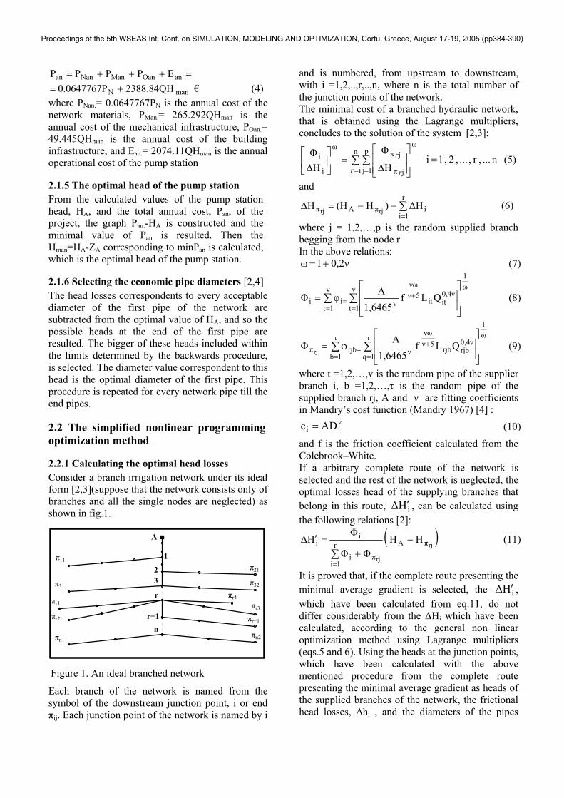
network, which is shown in fig. 2, is calculated. The material of the pipes is PVC 10 atm. The required minimal piezometric head at each node, hi, is resulted as it is described in paragraph 2.1.3. Figure 2 represents the real network and provide geometric and hydraulic details.

Figure 2. The real under solution network

3.1 Calculation according to the dynamic method

3.1.1 The optimal cost of the network The complete model of dynamic programming with backward movement (BDP, FDDP) is applied. The results are presented in table 1.

Table 1. The optimal cost of the network, PN , according to the dynamic programming method

HA [m] PN [€] HA [m] PN [€] HA m] PN [€] 83.74 395595 88.56 309127 93.24 27583984.02 384593 88.79 307246 93.38 27490884.73 364916 89.24 302955 94.06 27146685.00 360399 89.50 300660 94.49 26974685.25 353925 89.71 298800 95.04 26731385.49 349940 90.02 297106 95.48 26497485.79 345931 90.25 294676 95.99 26199386.01 341371 90.50 292930 96.48 26191386.25 338809 90.77 291689 97.06 26142986.48 334756 91.04 290119 97.57 26017086.76 330295 91.24 288481 97.89 25826687.00 327143 91.48 286134 98.79 25686987.23 324942 91.75 284619 99.78 25623287.48 321236 92.01 283533 100.24 25531987.75 319724 92.23 281717 100.86 25442188.06 316387 92.49 279850 102.57 25385888.25 312555 92.82 279005


3.1.2 The optimal head of the pump station Using the eq. 4, the total annual cost of the project is calculated for pump heads, HA, the values given in table 1. The results are presented in table 2. After all, the corresponding graphs Pan. - ΗA (fig.3) is constructed and the min Pan. is calculated. From the minPan. the corresponding Ηman = ΗA-ΖΑ is resulted.

Table 2. The total annual cost of the project, Pan. , according to the dynamic programming method

HA [m] Pan [€] HA [m] Pan [€] HA [m] Pan [€]83.74 44619 88.56 41907 93.24 4255084.02 44073 88.79 41920 93.38 4257184.73 43228 89.24 41911 94.06 4275985.00 43096 89.50 41919 94.49 4290585.25 42823 89.71 41922 95.04 4307385.49 42709 90.02 41999 95.48 4318785.79 42627 90.25 41978 95.99 4329986.01 42465 90.50 42016 96.48 4358386.25 42445 90.77 42095 97.06 4390086.48 42321 91.04 42160 97.57 4412686.76 42195 91.24 42175 97.89 4419787.00 42139 91.48 42166 98.79 4464087.23 42134 91.75 42227 99.78 4519287.48 42040 92.01 42313 100.24 4541287.75 42104 92.23 42327 100.86 4572388.06 42075 92.49 42360 102.57 4671288.25 41937 92.82 42500

From table 2 and fig.3 it is concluded that the minimal cost of the network is minPΕΤ. = 41907 €, produced for HA = 88.56 m with corresponding Hman = 88.56 – 52.00 = 36.56 m

3.2. Calculation according to the proposed simplified method

3.2.1 The variance of the head of the pump station

The complete route presenting the minimal average gradient is A-39. The minimal and maximal head losses of all the pipes, which belong to this complete route, are calculated and the results are shown in table 3. From the table is resulted that minHA=83.57 m and maxHA=102.59 m

Table 3. The minimal and maximal head losses of all the pipes, which belong to the complete route

presenting the minimal average gradient Minimal losses Maximal losses

Pipe Li [m] maxDi

[mm] min1.1Ji

[%] minDi [mm]

Max1.1Ji [%]

39 225 160 0.249 110 1.607

38 240 225 0.167 140 1.774 37 240 280 0.120 160 1.966 36 125 315 0.114 200 1.103 Κ36 190 450 0.071 250 1.342 K28 185 500 0.090 315 0.909 K19 120 500 0.194 355 1.083 K10 200 500 0.309 400 0.951 K1 50 500 0.450 450 0.766 A 0 0 0

3.2.2 The optimal total cost of the network The total minimal cost of the network, PN, is obtained using the eq. 12. The calculation is made for pump heads HA = 84.00 m till 102.00 m. The results are presented in table 4.

Table 4. The optimal cost of the network, PN , according to the simplified method

HA [m] PN [€] HA [m] PN [€] HA [m] PN [€]84 373921 91 280821 98 24224385 351530 92 273923 99 23808686 334153 93 267585 100 23443287 320064 94 261545 101 23105988 308244 95 256300 102 22764789 297889 96 251200 90 288850 97 246614

3.2.3 The optimal head of the pump station The total annual cost of the project is calculated using the eq. 4. The results are presented in table 5. After that, the corresponding graphs Pan-ΗA, (fig.3) is constructed and the minPan is calculated. From minPan the corresponded Ηman=ΗA-ΖΑ is resulted.

Table 5. The total annual cost of the project, Pan , according to the proposed simplified method

HA [m] PN [€] HA [m] PN [€] HA [m] PN [€] 84 43218 91 41465 98 43206 85 42385 92 41625 99 43541 86 41874 93 41821 100 43909 87 41573 94 42035 101 44295 88 41417 95 42301 102 44678 89 41355 96 42576 90 41378 97 42884

From table 5 and fig.3 it is resulted that the minimal cost of the network is minPΕΤ. = 41296 €, produced for HA = 89.05 m with corresponding Hman = 89.05 – 52.00 = 37.05 m Note: The value HA= 89.05 m have been resulted after the application of the above, for smaller subdivisions of HA values which are not presented in table 5.


40,50

41,50

42,50

43

3.3 Selecting the economic pipe diameters The economic diameters of the pipes are calculated according to the paragraphs 2.1.6 and 2.2.5. The results are presented in table 6.

Table 6. The optimal pipe diameters, DN , according to the both methods

DN [mm] DN [mm] Pipe Length

[m] Dyn. Meth

Simpl.Meth

Pipe Length [m] Dyn.

MethSimpl.Meth

Κ1 50 452.2 424 22 250 126.6 1221 140 144.6 141 23 120 180.8 184 2 280 126.6 126 24 230 180.8 173 3 350 113.0 104 25 230 180.8 160 4 120 203.4 194 26 255 144.6 143 5 235 180.8 184 27 165 99.4 118 6 240 180.8 173 Κ28 185 321.2 3077 230 180.8 160 28 185 203.4 187 8 210 126.6 143 29 240 180.8 173 9 160 126.6 118 30 235 144.6 155 Κ10 200 407.0 393 31 255 126.6 128 10 135 144.6 145 32 125 180.8 170 11 290 144.6 130 33 225 180.8 157 12 245 99.4 107 34 235 144.6 140 13 120 203.4 198 35 225 99.4 116 14 235 180.8 188 Κ36 190 253.2 26315 235 180.8 177 36 125 203.4 20316 230 180.8 163 37 240 203.4 18717 210 144.6 146 38 240 180.8 16718 145 126.6 120 39 225 126.6 138Κ19 120 361.8 358 40 120 203.4 179 19 230 180.8 180 41 240 180.8 165 20 240 180.8 166 42 225 144.6 147 21 250 144.6 148 43 300 133.0 122

,50

44,50

45,50

46,50

83 85 87 89 91 93 95 97 99 101 103

Note: The above calculated diameters from the simplified method necessarily must be rounded off to the nearest available higher commercial size.

Figure 3.

4. CONCLUSIONS The optimal head of the pump station that

results, according to the dynamic programming method is Hman = 36.56 m, while according the proposed simplified method is Hman = 37.05 m. These two values differ only 1.34% while the corresponding difference in the total annual cost of the project is only 1.48 %.

The two optimization methods in fact conclude to the same result and therefore can be applied with no distinction in the studying of the branched hydraulic networks.

The required calculating procedure for the determination of the available piezometric losses is much shorter when using the simplified method than when using the dynamic programming optimization method. Therefore the proposed simplified method is indeed very simple to handle and for practical uses it requires only a handheld calculator and just a few numerical calculations.

References: [1] Labye, Y., Etude des procedés de calcul ayant

pour but de rendre minimal le cout d’un reseau de distribution d’eau sous pression, La Houille Blanche,5: 577-583, 1966.

[2] Theoharis, M.,“Βελτιστοποίηση των αρδευτικών δικτύων. Επιλογή των οικονοµικών διαµέτρων”, Ph.D. Thesis, Dep. of Rural and Surveying Engin. A.U.TH., Salonika, 2004 (In Greek).

[3] Tzimopoulos, C. “Γεωργική Υδραυλική” Vol. II, 51-94, A.U.TH., Salonika, (In Greek),1982.

[4] Vamvakeridou-Liroudia L.,"∆ίκτυα υδρεύσεων - αρδεύσεων υπό πίεση. Επίλυση – βελτιστοποίη-ση", Athens, (In Greek),1990.

[5] Yakowitz, S., Dynamic programming applica-tions in water resources, Journal Water Resources. Research, Vol. 18, Νο 4, Aug. 1982, pp. 673- 696.

Tota

l ann

ual c

ost o

f the

pr

ojec

t P

an [x

103 €

] Dynamic method [6] Walters, G, A., and McKechnie S.J., Determi-

ning the least-cost spanning network for a system of pipes by the use of dynamic programming, Proc. 2nd Int. Conf. οn Civil & Structural Eng. Computing, London, Dec. 1985, pp. 237-243.

Simplified method

[7] Yang Κ.P., Liang Τ., and Wu Ι.P., Design of conduit systems with diverging branches, ]


Pump station head HA [m

Variance of Pan per HA.

Journal. Hydr. Div., ASCE, Vo1.101, Νο 1, Jan. 1975, pp. 167-188..


Documents

OPTIMAL DESIGN OF IRRIGATION NETWORKS USING THE …OPTIMAL DESIGN OF IRRIGATION NETWORKS USING THE DYNAMIC METHOD AND A SIMPLIFIED NONLINEAR METHOD ... in the management of the water