Embed Size (px)
Citation preview

1
OPTIMAL DESIGN OF HYBRID ELECTRIC VEHICLE by
Shifang Li Prasad Challa Rajit Johri
Girish Chandra
MECHENG/MFG 555
Winter 2008
Final Report
Abstract Stringent emission regulations combined with customer demands for improved fuel
economy and performance have forced the automotive industry to consider more
advanced powertrain configurations. Modern state‐of‐the‐art powertrain systems may
combine several power sources ‐ electric motors, fuel cells and modern engines based
on HCCI or PCI technologies. This project aims at reducing the fuel consumption for
Hybrid Electric Vehicle, HEV by optimizing the component design and size. HEVs exploit
the capacity of an additional energy source aboard to reduce the modulation of the
primary energy source (engine). This allows a reduction of fuel consumption and a
better sizing for the primary engine. The determination of the way in which these
systems have to be sized to meet driver’s torque demand, performance and fuel
economy expectations while satisfying federal emission regulations is a complex
optimization problem.
The vehicle was divided into four subsystems ‐ engine, automatic transmission, electrical
machinery and propulsion shafts and each subsystem was optimized individually. A fuel
economy of about 68% was obtained after complete system optimization.
2
Table of Contents
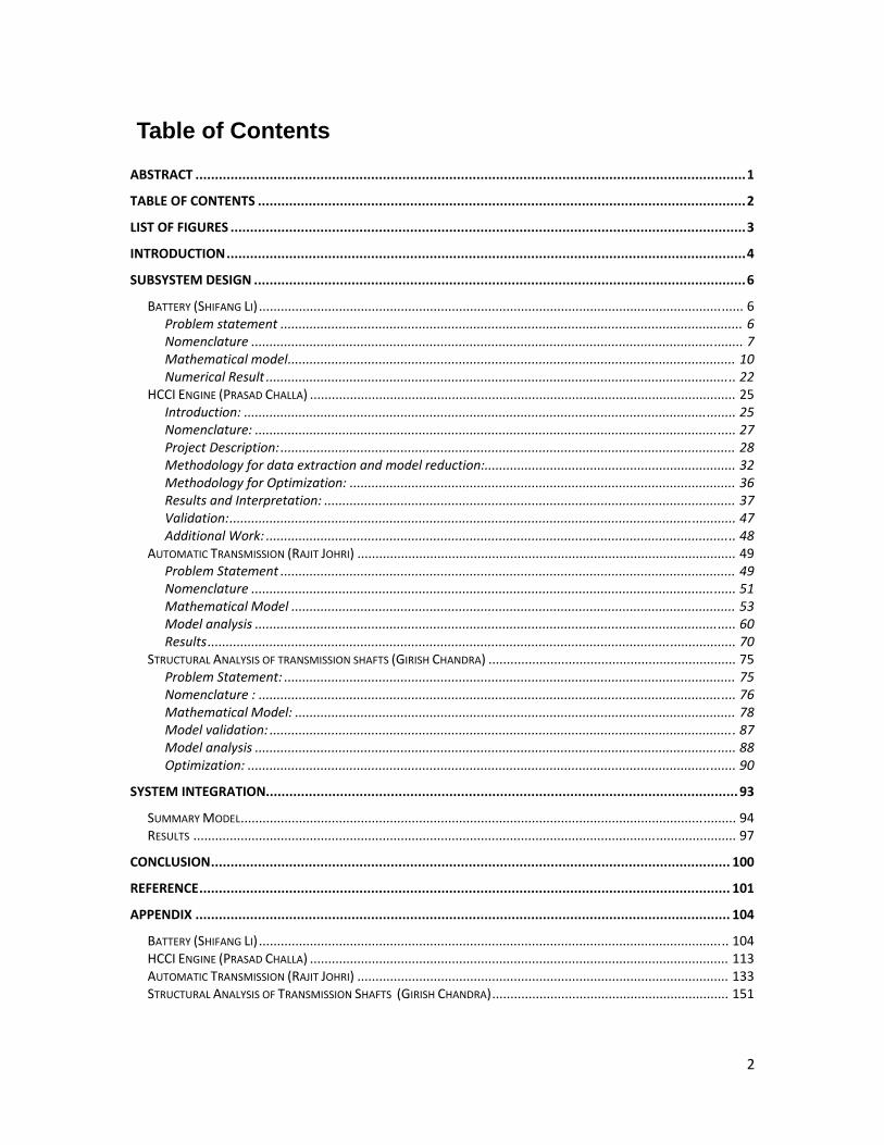
ABSTRACT ............................................................................................................................................. 1
TABLE OF CONTENTS ............................................................................................................................. 2
LIST OF FIGURES .................................................................................................................................... 3
INTRODUCTION ..................................................................................................................................... 4
SUBSYSTEM DESIGN .............................................................................................................................. 6
BATTERY (SHIFANG LI) ..................................................................................................................................... 6 Problem statement ............................................................................................................................... 6 Nomenclature ....................................................................................................................................... 7 Mathematical model ........................................................................................................................... 10 Numerical Result ................................................................................................................................. 22
HCCI ENGINE (PRASAD CHALLA) ..................................................................................................................... 25 Introduction: ....................................................................................................................................... 25 Nomenclature: .................................................................................................................................... 27 Project Description: ............................................................................................................................. 28 Methodology for data extraction and model reduction:..................................................................... 32 Methodology for Optimization: .......................................................................................................... 36 Results and Interpretation: ................................................................................................................. 37 Validation: ........................................................................................................................................... 47 Additional Work: ................................................................................................................................. 48
AUTOMATIC TRANSMISSION (RAJIT JOHRI) ........................................................................................................ 49 Problem Statement ............................................................................................................................. 49 Nomenclature ..................................................................................................................................... 51 Mathematical Model .......................................................................................................................... 53 Model analysis .................................................................................................................................... 60 Results ................................................................................................................................................. 70
STRUCTURAL ANALYSIS OF TRANSMISSION SHAFTS (GIRISH CHANDRA) .................................................................... 75 Problem Statement: ............................................................................................................................ 75 Nomenclature : ................................................................................................................................... 76 Mathematical Model: ......................................................................................................................... 78 Model validation: ................................................................................................................................ 87 Model analysis .................................................................................................................................... 88 Optimization: ...................................................................................................................................... 90
SYSTEM INTEGRATION......................................................................................................................... 93
SUMMARY MODEL ........................................................................................................................................ 94 RESULTS ..................................................................................................................................................... 97
CONCLUSION ..................................................................................................................................... 100
REFERENCE ........................................................................................................................................ 101
APPENDIX ......................................................................................................................................... 104
BATTERY (SHIFANG LI) ................................................................................................................................. 104 HCCI ENGINE (PRASAD CHALLA) ................................................................................................................... 113 AUTOMATIC TRANSMISSION (RAJIT JOHRI) ...................................................................................................... 133 STRUCTURAL ANALYSIS OF TRANSMISSION SHAFTS (GIRISH CHANDRA) ................................................................. 151
3
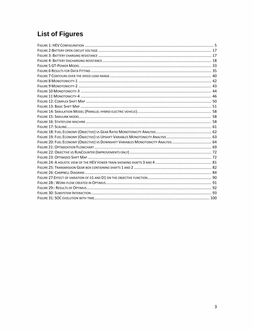
List of Figures FIGURE 1: HEV CONFIGURATION ........................................................................................................................... 5 FIGURE 2:BATTERY OPEN CIRCUIT VOLTAGE ............................................................................................................ 17 FIGURE 3: BATTERY CHARGING RESISTANCE ............................................................................................................ 17 FIGURE 4: BATTERY DISCHARGING RESISTANCE ........................................................................................................ 18 FIGURE 5 GT‐POWER MODEL ............................................................................................................................. 33 FIGURE 6 RESULTS FOR DATA FITTING ................................................................................................................... 35 FIGURE 7 CONTOURS OVER THE SPEED LOAD RANGE ................................................................................................. 40 FIGURE 8 MONOTONICITY‐1 ............................................................................................................................... 42 FIGURE 9 MONOTONICITY‐2 ............................................................................................................................... 43 FIGURE 10 MONOTONICITY‐3 ............................................................................................................................. 44 FIGURE 11 MONOTONICITY‐4 ............................................................................................................................. 46 FIGURE 12: COMPLEX SHIFT MAP ........................................................................................................................ 50 FIGURE 13: BASIC SHIFT MAP ............................................................................................................................. 51 FIGURE 14: SIMULATION MODEL (PARALLEL HYBRID ELECTRIC VEHICLE) ....................................................................... 58 FIGURE 15: SIMULINK MODEL .............................................................................................................................. 58 FIGURE 16: STATEFLOW MACHINE ........................................................................................................................ 58 FIGURE 17: SCALING .......................................................................................................................................... 61 FIGURE 18: FUEL ECONOMY (OBJECTIVE) VS GEAR RATIO MONOTONICITY ANALYSIS ..................................................... 62 FIGURE 19: FUEL ECONOMY (OBJECTIVE) VS UPSHIFT VARIABLES MONOTONICITY ANALYSIS ........................................... 63 FIGURE 20: FUEL ECONOMY (OBJECTIVE) VS DOWNSHIFT VARIABLES MONOTONICITY ANALYSIS ...................................... 64 FIGURE 21: OPTIMIZATION FLOWCHART ................................................................................................................ 69 FIGURE 22: OBJECTIVE VS RUNCOUNTER (IMPROVEMENTS ONLY) .............................................................................. 72 FIGURE 23: OPTIMIZED SHIFT MAP ...................................................................................................................... 72 FIGURE 24: A HOLISTIC VIEW OF THE HEV POWER TRAIN SHOWING SHAFTS 3 AND 4 ...................................................... 81 FIGURE 25: TRANSMISSION GEAR BOX CONTAINING SHAFTS 1 AND 2 .......................................................................... 82 FIGURE 26: CAMPBELL DIAGRAM ......................................................................................................................... 84 FIGURE 27:EFFECT OF VARIATION OF D1 AND D1 ON THE OBJECTIVE FUNCTION. ............................................................ 90 FIGURE 28:: WORK‐FLOW CREATED IN OPTIMUS ..................................................................................................... 91 FIGURE 29:: RESULTS OF OPTIMUS ....................................................................................................................... 92 FIGURE 30: SUBSYSTEM INTERACTION ................................................................................................................... 93 FIGURE 31: SOC EVOLUTION WITH TIME .............................................................................................................. 100

4
Introduction With the growing demand from the world community to reduce the emission of carbon
dioxide, and after a decade of intense research, hybrid electric vehicles (HEV) suddenly
appear more viable and necessary than ever before. These vehicles either reduce or
eliminate the reliance on fossil fuels. Owing to their dual on‐board power sources and
regenerative braking, HEVs offer unprecedented possibilities to pursue higher fuel
economy.
Conventional internal combustion (IC) engine‐driven powertrains have several
disadvantages that negatively affect fuel economy and emissions. Specifically, IC engines
are over designed to meet performance targets such as acceleration and gradeability.
Oversizing the engine moves the operating point away from optimal operation point.
Moreover, engine cannot be optimized for all loads and speed ranges under which it
must operate. A parallel HEV allows engine and the motor to drive the vehicle
simultaneously or independently. Hence engine can be downsized to reduce fuel
consumption and emission. Also overall control strategy can be developed which allows
engine to operate in a desired speed‐load range.
Work on hybrid powertrain optimization has been carried out previously using variety of
optimization model and simulations. Moore et al [1] carried out parametric studies to
assess component size based on continuous and peak demand of power and torque.
Zoelch et al. [2]used dynamic optimization to calculate optimal electric motor torque,
engine torque and CVT gear ratios for a parallel HEV under simple charge‐neutral driving
cycles. Recently detailed optimization study on EPA driving cycles has been carried out
by Assanis et al [3].
The design process requires a system engineering approach, in which the design of each
component must be evaluated through the component’s contribution to the overall
system performance. The design process typically starts with evaluation of trade‐offs
associated with component sizes for a targeted fuel economy and performance. Fuel
economy and performance of the vehicle presents a trade‐off in system design. Bigger
5
engine and higher rating motor with large battery pack will result in improved
performance but will incur penalty on fuel economy due to increased weight. Similarly
smaller engine and reduced battery pack will help in better fuel economy at the cost of
performance. Hence the vehicle system has trade‐off between fuel economy and
performance. This is the motivation for figuring out the optimal component sizing.
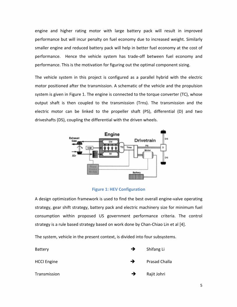
The vehicle system in this project is configured as a parallel hybrid with the electric
motor positioned after the transmission. A schematic of the vehicle and the propulsion
system is given in Figure 1. The engine is connected to the torque converter (TC), whose
output shaft is then coupled to the transmission (Trns). The transmission and the
electric motor can be linked to the propeller shaft (PS), differential (D) and two
driveshafts (DS), coupling the differential with the driven wheels.
Figure 1: HEV Configuration
A design optimization framework is used to find the best overall engine‐valve operating
strategy, gear shift strategy, battery pack and electric machinery size for minimum fuel
consumption within proposed US government performance criteria. The control
strategy is a rule based strategy based on work done by Chan‐Chiao Lin et al [4].
The system, vehicle in the present context, is divided into four subsystems.
Battery Shifang Li
HCCI Engine Prasad Challa
Transmission Rajit Johri

6
Structural Dynamics of propulsion shaft Girish Chandra
All the subsystems in vehicle are interconnected and cannot be optimized individually
without affecting the other subcomponent. However, in this project, all subcomponents
are optimized independently with nominal values for other subsystem parameters.
Overall system optimization will be carried out later with optimized components to
arrive at a system wide solution.
Subsystem Design
Battery (Shifang Li)
Problem statement
Hybrid electric vehicle has two power sources, one is the engine and the other is the
battery. The existence of the battery in the hybrid electric vehicle (HEV) is the main
feature of HEV compared to conventional vehicles, and it is the very reason why HEV
outperforms conventional vehicles in fuel economy and low emissions. When the power
command is low, the battery alone drives the vehicle, when the power demand is
medium, the battery cushions the vehicle power fluctuations, thus make the engine
always work in efficient regions, which will contribute to fuel economy and low
emission. And the battery supplies power for peak demands when the power command
exceeds the maximum power of the engine. In this case, the battery contributes to the
improvement of the vehicle performance. Furthermore, the battery also absorbs
current during regenerative braking events, thus capturing this valuable energy that is
dissipated and lost in a conventional vehicle.
Hybrid vehicle operation puts unique demands on the battery when it operates as the
auxiliary power source. In order to optimize its operating life, the battery must spend
minimum time in overcharge and/or overdischarge. HEV batteries, in current designs,

7
have voltages of 100‐300 V, or more. As noted above, the battery must be capable of
furnishing or absorbing large currents almost instantaneously while operating around a
partial‐state‐of‐charge baseline of roughly 50% [5]. If we have a very big battery,
obviously, it is easier for the state of charge to stay near the partial‐state‐of‐charge
baseline, since the power from or to the battery is relatively small to its capacity.
Therefore, a big battery will have better operating conditions and consequently a longer
operating life.
While at the mean time, vehicle total mass has an important influence on vehicle
performance. Hybrid electric vehicle mileage increases dramatically as vehicle mass
decreases[6]. The battery weight makes a great portion of the whole mass of the
vehicle, optimization of the battery mass is of great importance for reducing fuel
consumption, and also smaller battery lowers the cost. So the trade off here for the
battery is satisfying the power command, containing a good operating condition while
possessing less weight.
The NiMH battery in ADVISOR is employed for the optimization design. The battery is
composed of battery modules, which are composed of battery cells. The battery is
modeled as a static equivalent circuit[7]. The rule based power management strategy is
applied to this model. The optimization design objective is to minimize the battery mass,
which mainly determined by the number of modules in the battery.
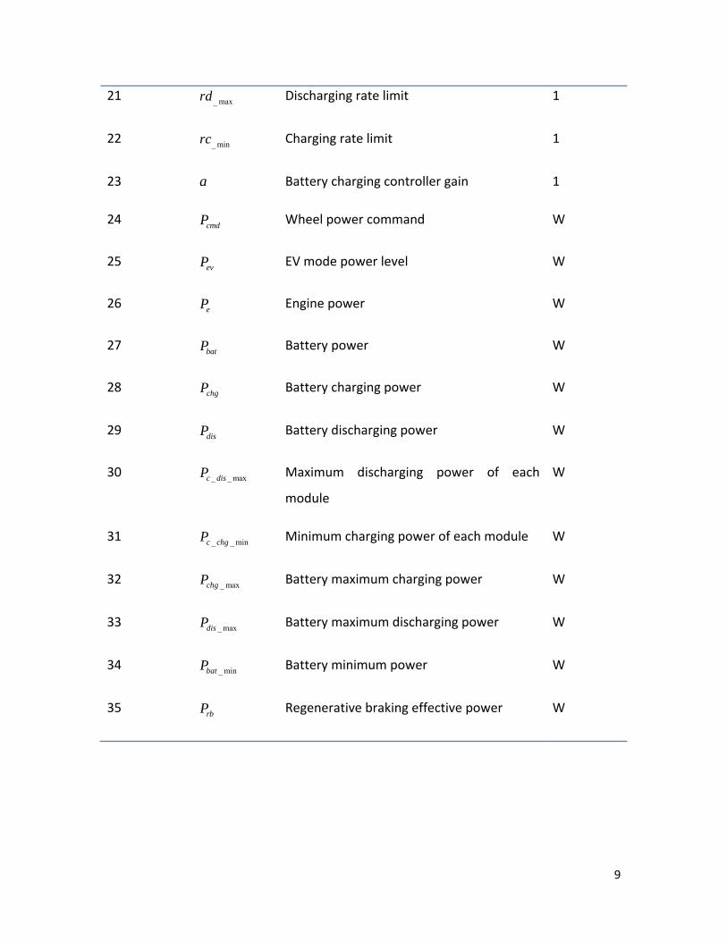
Nomenclature
Index Symbol Description Unit
1 _c batC Capacity of each module Ah
2 n Number of modules 1

8
3 m Module mass kg
4 γ Mass packaging factor 1
5 batV Battery voltage Volt
6 maxV Battery maximum voltage Volt
7 ocV Open circuit voltage volt
8 batI Battery current Amp
9 chgI Battery charging current Amp
10 disI Battery discharging current Amp
11 _ minchgI Maximum charging current Amp
12 _ maxdisI Maximum discharging current Amp
13 dR Discharging resistance ohms
14 cR Charging resistance ohms
15 s State of charge 1
16 maxs Maximum SOC 1
17 mins Minimum SOC 1
18 dess Desired SOC 1
19 sd
Changing rate of SOC 1
20 _ minrrb Regenerative braking charging rate limit 1
9
21 _ maxrd Discharging rate limit 1
22 _ minrc Charging rate limit 1
23 a
Battery charging controller gain 1
24 cmdP Wheel power command W
25 evP EV mode power level W
26 eP Engine power W
27 batP Battery power W
28 chgP Battery charging power W
29 disP Battery discharging power W
30 _ _ maxc disP Maximum discharging power of each
module
W
31 _ _ minc chgP Minimum charging power of each module W
32 _ maxchgP Battery maximum charging power W
33 _ maxdisP Battery maximum discharging power W
34 _ minbatP Battery minimum power W
35 rbP Regenerative braking effective power W

10
Mathematical model
1. Objective function
The objective of the optimization design is to minimize the battery mass for the
objective of the whole vehicle to have optimal mileage, while at the same time
maintain the battery to operate at good conditions for the sake of its operating
life.
Objective function:
min n m γ× ×
2. Constraints:
a) Physical Constraints
The battery has to operate at its healthy region, the power, current and voltage
should never exceed its limit.
_ max( , , , )chg chg rb ev chgP SOC SOC P P P− ≤
_ max( , , , )dis chg rb ev disP SOC SOC P P P− ≤
_ max 0ev disP P− ≤
_ min 0bat rbP P− ≤
_ max ( ) 0chg bat batI I P− ≤
_ max( ) 0bat bat disI P I− ≤
max( ) 0bat batV P V− ≤
1( )ocV f SOC=

11
2 ( )disR f SOC=
( )3chgR f SOC=
00
d bat
c bat
R PR
R P≥⎧
= ⎨ <⎩
2 4
2ococ bat
bat
V V RPI
R
− −=
2 4
2ococ bat
bat
V V RPV
+ −=
2 4
2ococ bat
bat
V V RNsd
RC
− −= −
_ max _ _ maxchg m chgP n P= ×
_ max _ _ maxdis m disP n P= ×
b) Practical Constraints
The state of charge of the battery should maintain in a range which will not
damage the battery. The charging and discharging efficiency should be less than
the EV mode power level should be less than the maximum power of the battery
and the regenerative braking effective power should be larger than the minimum
power of the battery which indeed is large enough to charge the battery. And the
open circuit voltage and discharging and charging resistance are functions of the
state of charge. The function will be obtained based on curve fitting of the
experimental data in PSAT.
_ min 0rrrb sd− ≤

12
_ min 0crc sd− ≤
_ max 0dsd rd− ≤
0n− ≤
200 0n− ≤
10000 0a− ≤
200000 0a − ≤
0.3 0s− ≤
0.9 0s − ≤
1000 0eP− ≤
40000 0eP − ≤
40000 0rP− − ≤
0rP ≤
minif SOC SOC≤
0disP =
( )chg chgP s sα= −
bat chgP P=
min maxif s s s< <
0rb cmdif P P< ≤

13
0disP =
0chgP =
0batP =
cmd rbif P P≤
0disP =
chg cmdP P=
bat chgP P=
0 cmd evif P P< ≤
dis cmdP P=
0chgP =
bat disP P=
max&cmd ev cmd eif P P P P> <
( )chg chgP s sα= −
dis chgP P= −
bat chgP P=
maxcmd eif P P≥
maxdis cmd eP P P= −
0chgP =

14
bat disP P=
maxif s s>
0cmdif P ≤
0disP =
0chgP =
0batP =
0 cmd evif P P< ≤
dis cmdP P=
0chgP =
bat disP P=
max&cmd ev cmd eif P P P P> <
( )chg chgP a s s= −
dis chgP P= −
bat chgP P=
maxcmd eif P P≥
maxdis cmd eP P P= −
0chgP =
bat disP P=
15
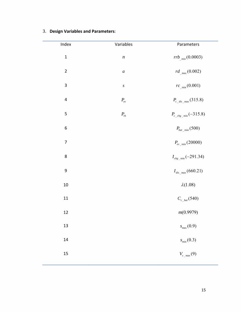
3. Design Variables and Parameters:
Index Variables Parameters
1 n _ min (0.0003)rrb
2 a _ max (0.002)rd
3 s _ min (0.001)rc
4 evP _ _ max (315.8)c disP
5 rbP _ _ min ( 315.8)c chgP −
6 _ min (500)batP
7 _ min (20000)evP
8 _ min ( 291.34)chgI −
9 _ max (660.21)disI
10 (1.08)λ
11 _ (540)c batC
12 (0.9979)m
13 max (0.9)s
14 min (0.3)s
15 _ max (9)cV

16
4. Model Simplification
In practice, the battery will work on different conditions due to the current state
of charge and the power command from or to the battery, as stated in the
practical constraints in the model above. While for our optimization purpose,
some of the conditions will be dominated by the extreme conditions, that is,
some of the constraints are inactive. For the battery voltage, the possible
maximum value will be reached when the battery is being charged and the
current state of charge is at the minimum. So this is one of the dominant cases
for battery voltage constraint. Another dominant case is when the battery is
charged by regenerative braking, the minimum wheel command power will
contribute to the possible maximum battery voltage. Similar with battery
voltage, for the battery current, the possible maximum current will be reached
when the battery is being charged at minimum state of charge or when the
wheel power command reached minimum. For the battery power, the maximum
discharging power will be reached when the battery power from the battery
reached the maximum value in a driving cycle, and the possible maximum
charging power also occurs when the minimum regenerative braking power or
maximum charging power from the engine are reached. Therefore, we can
simplify the model by eliminating the different operation conditions stated in the
practical constraints in the model above and considering only the dominant
conditions, which result in the summary model bellow.
In order to get the functions of the battery open circuit voltage, discharging
resistance and charging resistance of the battery module. I applied curve fitting
to the experimental data of the battery of Toyota Pirus[8]. The battery open
circuit voltage is approximated by third order polynomial, while the discharging
and charging resistance are approximated by fourth and third order respectively.
5 4 3 2(17.29 37.172 29.323 10.977 2.6624 7.2332)ocV n s s s s s= − + − + +

17
4 3 2(0.01486 0.05091 0.08153 0.05206 0.03783)dR n s s s s= − + − +
3 2( 0.0149 0.031987 0.020225 0.023541)cR n s s s= − + − +
The curve fitting figure is showing below.
Figure 2:Battery open circuit voltage
Figure 3: Battery charging resistance

18
Figure 4: Battery discharging resistance
5. Summary model
min n m γ× ×
Subject to:
g1: _ _ max 0ev c disP nP− ≤
g2: _ _ min 0c chg rbnP P− ≤
g3: _ _ min ( 0.5) 0c chgnP α− − ≤
g4: 2
_ max
40
2oc oc ev
dis
V V RPI
R− −
− ≤
g5: 2
_ min
40
2ococ rb
chg
V V RPI
R
− −− ≤
g6: 2
_ max
40
2ococ rb
c
V V RPnV
+ −− ≤
g7: 2
_ min_
40
2oc rb oc
c bat
V RP Vrrb
RnC
− −− ≤

19
g8: 2
_ min_
4 ( 0.1)0
2oc oc
c bat
V R Vrc
RnC
α− − −− ≤
g9: 2
_ max_
40
2oc ev oc
c bat
V RP Vrd
RnC
− −− − ≤
g10: 0n− ≤
g11: 200 0n− ≤
g12: 10000 0a− ≤
g13: 200000 0a − ≤
g14: 0.3 0s− ≤
g15: 0.9 0s − ≤
g16: 15000 0eP− ≤
g17: 40000 0eP − ≤
g18: 40000 0rP− − ≤
g19: _ min 0r batP P+ ≤
h1: 5 4 3 2(17.29 37.172 29.323 10.977 2.6624 7.2332) 0ocV n s s s s s− − + − + + =
h2: 4 3 2(0.01486 0.05091 0.08153 0.05206 0.03783) 0dR n s s s s− − + − + =
h3: 3 2( 0.0149 0.031987 0.020225 0.023541) 0cR n s s s− − + − + =

20
6. Model Analysis
The model reduction is done in part 3 (4) model simplification, and no further
reduction can be made based on monotonicity analysis. Because the constraints
are nonlinear and very complex, explicit solutions with respect to the variables
cannot be found. However, in order to reduce computation burden, Taylor series
are employed to approximate the nonlinear constraints to quadratic form. The
nonlinear constraints become following.
g4: 2
2
2_ max
61.9628 2.25016 0.0258965 0.00675047
0.0000987605 6.32135 8 30.2269
0.0242916 0.0000728748 24.6996 0
ev
ev ev
ev dis
n n P
nP e P s
ns P s s I
− + +
− + − −
− + + − ≤
g5: 2
_ min
2
2
11.8682 0.355285 0.00276912 0.00413003
0.0000323878 1.00993 8 3.14753 0.0242916
0.0000691885 1.40955 0
chg r
r r
r
I n n P
nP e P s ns
P s s
+ − + −
+ − − − +
+ + ≤
g6: 2
2
2_ max
22.884 7.59686 0.00008291 - 0.00231361.9898510 6 1.19391 8 76.28220.24673 0.000171785 63.5685 0
r
r r
r c
n n PnP e P s
ns P s s nV
− + −
− − − − +
+ − − − ≤
g7: 2
_ min
2
2
(0.000999444 0.0000321704 2.63007 7 1.90564
7 2.05119 9 3.11705 13 0.0000734718
3.55172 7 2.13545 9 0.0000435047 ) 0r r r
r
rrb n e n
e P e nP e P s
e ns e P s s
− − + − −
− + − − − −
+ − + − + ≤
g8: 2
_ min
2
2
(0.000999444 0.0000321704 2.63007 7 1.14338
7 1.23071 9 1.12214 13 0.0000734718 3.551727 1.28127 9 0.0000435047 ) 0
rc n e n e
a e na e a s ens e as s
− − + − +
− − − − − − +
− − − + ≤
g9: 2
2
2_ max
( 0.00517751 0.000185935 1.83374 6 3.13197 7
4.79564 9 1.95103 12 0.000951056 4.47576
7 2.24922 9 0.00076233 ) 0
e
e e
e
n e n e P
e nP e P s e
ns e P s s rd
− − + − − − −
+ − − − + +
− − − − − ≤

21
Optimization approach:
(1) Based on the quadratic form constraints, and the original constraints, the
function ‘fmincon’ in Matlab is applied to solve the optima. And the scaling of
the variables and the constraints are implemented. Corresponding to
different initial guess, the optimal result is different. And since the feasible
space has very irregular bounders due to the existence of coupled term
under square root, the result easily goes into the infeasible space or just
converges to a local minima. The Matlab code is in part 7.
(2) The nonlinear constraints are linearized by Taylor’s expansion in order to
avoid the inconvenience of the irregular bounders of the feasible space in the
optimization approach (1) to transform the problem into a linear
programming problem. The function ‘linprog’ is employed to solve the
optimization problem. The matlab code is in part 7.
The linearized model is summarized as following:
min n m γ× ×
Subject to:
g1: 315.8 0evP n− ≤
g2: 315.8 0rbn P− − ≤
g3: 315.8 0.5 0n a− + ≤
g4: 598.2472 2.25016 0.00675047 30.2269 0evn P s− − + − ≤
g5: 279.4718 0.355285 0.00413003 3.14753 0rn P s− − − − ≤
g6: 22.884 1.4031 0.0023136 76.2822 0rn P s− − − + ≤
22
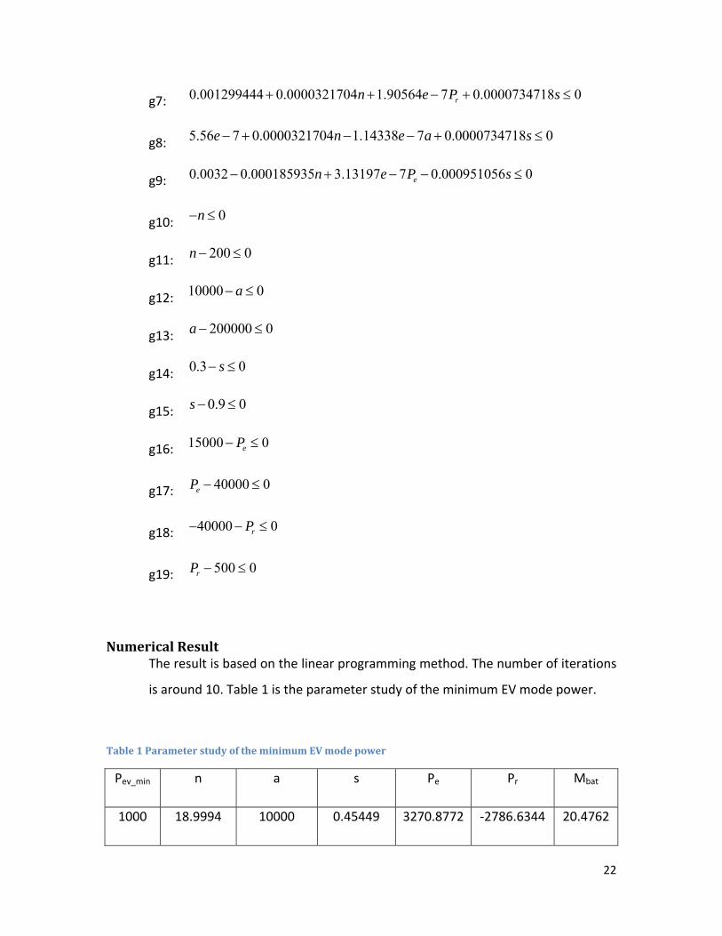
g7: 0.001299444 0.0000321704 1.90564 7 0.0000734718 0rn e P s+ + − + ≤
g8: 5.56 7 0.0000321704 1.14338 7 0.0000734718 0e n e a s− + − − + ≤
g9: 0.0032 0.000185935 3.13197 7 0.000951056 0en e P s− + − − ≤
g10: 0n− ≤
g11: 200 0n− ≤
g12: 10000 0a− ≤
g13: 200000 0a − ≤
g14: 0.3 0s− ≤
g15: 0.9 0s − ≤
g16: 15000 0eP− ≤
g17: 40000 0eP − ≤
g18: 40000 0rP− − ≤
g19: 500 0rP − ≤
Numerical Result The result is based on the linear programming method. The number of iterations
is around 10. Table 1 is the parameter study of the minimum EV mode power.
Table 1 Parameter study of the minimum EV mode power
Pev_min n a s Pe Pr Mbat
1000 18.9994 10000 0.45449 3270.8772 ‐2786.6344 20.4762

23
3000 18.994 10000 0.46784 4447.0823 ‐3.59.364 20.4762
5000 18.9994 10000 0.49878 5392.9236 ‐3968.0021 20.4762
6000 18.9994 10000 0.50168 6000 ‐3894.555 20.4762
7000 22.1659 10848 0.53562 7000 ‐4639.9712 23.8889
9000 28.4991 12235.4176 0.47208 9000 ‐4354.9471 30.7143
10000 31.6656 12891.3332 0.53799 10000 ‐5702.6437 34.127
12000 37.9987 14521.2646 0.68994 12000 ‐7793.9693 40.9525
14000 44.3319 15701.18 0.82716 14000 ‐6757.9139 47.7779
16000 50.665 18415.5397 0.734 16000 ‐7202.1006 54.6033
18000 56.9981 21141.2116 0.72554 18000 ‐8088.7489 61.4287
20000 63.3312 29769.2059 0.54387 20000 ‐9954.1539 68.2514
21000 66.4978 22878.7827 0.57993 21000 ‐8942.3169 71.6668
The battery EV mode power is set to be the maximum power the battery should
be able to provide. And it contributes to the activity of the constraint for
maximum discharging rate. As we can see from the table, when the minimum EV
mode power is larger than 5 KW, the EV mode power equals to the minimum EV
mode power. In reality, the EV mode power is around 10KW. As the minimum EV
mode power becomes larger, the number of modules in the battery pack
increases as anticipated, because larger battery which contains more modules
can provide more power. When the number of modules in the battery increases,
we need to increase the controller gain to satisfy the minimum charging rate
from the engine power. While for the desired state of charge, it depends on the
battery type. Because the functions of open circuit voltage, charging and

24
discharging resistance are based on the experimental data of the specific NiMH
battery, the optimization result can only be interpreted as that for a specific
power command scenario, such as a driving cycle, the set point of the desired
state of charge as shown in the table above will provide the best efficiency of the
battery. We see that the optimization result of the desired state of charge is
around the middle point of the cap of the state of charge, except very few points
which reached 0.8. The reason for the deviation of the few points may be due to
the polynomial approximation error or even the experimental error. Generally, it
is consistent with the actual healthy and efficient region of the battery. As for
the regenerative braking, we know that larger start value of the regenerative
braking power (one should notice that the regenerative braking power is
negative) will make more usage of the braking and contribute to fuel efficiency.
However, the battery has a power limit below which the power applied to the
battery will have no effect. And for engineering practical application, we have a
minimum charging rate for regenerative braking, and this condition may impose
another constraint for the maximum regenerative braking power. From the
optimization result, we see that the minimum charging rate do provide an active
constraint. Therefore, the optimization result is reasonable, and it provides the
optimal set points for the variables in the battery and battery controller design.
And since the number of modules in the battery pack should be an integer, we
have to choose the least integer larger than the optimal value of the battery
number.

25
HCCI Engine (Prasad Challa)
Introduction:
In light of the stringent norms on the emissions pertaining to the vehicles, the present
automakers have put their focus primarily on the fuel economy improvement of the
vehicle as well as meeting the emission standards of the vehicle. This is due to the fact
that the vehicle‐out emissions per mile travelled are a direct function of the emission
per unit fuel consumed and the fuel economy of the vehicle.
The improvement in the fuel economy has taken new strides through these years with
the successful elimination of the throttle in an SI engine using advanced technologies
like DISI, which give more flexibility to go to higher compression ratios thus boosting the
performance. The same is true on the Diesel side too with variable valve strategy being
applied to the Diesel engine to boost the performance. In addition to these, the
introduction of turbochargers and superchargers has improved the efficiency of these
engines greatly.
In spite of all these efforts towards improvement in the fuel economy, the vehicle
suffers from the non‐conformance to the emission standards in these vehicles. Though
there has been a lot of significant improvement in the emissions field too, the after‐
treatment devices remain pretty costly. One main problem faced on the emissions front
is the inverse relation of the soot and NOx emissions. The only way to deal with this
problem is to have cooler combustion of a homogeneous charge. This is precisely
achieved by the Homogeneous Charge Compression Ignition (HCCI) engine.
Problem Statement:
The engine of interest in the present project is a 4‐cylinder HCCI engine operated on a
variable valve‐train. HCCI engine is different from the conventional SI and CI engines in
its ignition characteristics. The mixture in a HCCI engine is homogeneous and there is no

26
direct trigger for the initiation of combustion in the engine. The heated residual gas of
the previous cycle is utilized to trigger the combustion in the present cycle. One way to
change the combustion characteristics of the engine is to alter the residual gas trapped
in the cylinder so as to control the combustion timing and duration. This is enabled by a
flexible valve‐train strategy through the change of valve lift, timing and valve duration.
Another object of interest in the present study is the intake charge temperature in the
way it affects the temperature at TDC thus affecting the combustion phasing.
The HCCI engine will be modeled in GT‐Power, commercial software for engine
modeling. The HCCI engine used for the project is developed as a part of research work
at Automotive Research Center (ARC). A typical recompression valve strategy 102will be
dealt with as a part of the present project. The valve lift, duration and timing will be
manipulated to adjust the residual gas trapped in the cylinder. The performance of any
engine depends on several conflicting variables, the main hindrances being knocking
and emissions [2]. For the HCCI engine, because of its unconventional way of combustion,
the range of operation is limited and hence cannot operate at all loads and speeds. All
these factors affect the performance of the engine a great deal and partly negate the
performance benefits of using a HCCI engine. The modeling objective of the present
study is the minimization of the fuel consumption, meeting all the emission
requirements and avoiding the engine knock, through the use of variable valve‐train,
over a particular drive cycle. The optimization of other sub‐systems will be dealt by
having engine maps as a function of the variables of interest.
The residual gas fraction of the engine can be successfully manipulated to be at the
desired level for each load so as to have the combustion at its optimal point (50% burn
angle at around 5‐10). However with the increase in the load of the engine, the rate of
pressure rise increases in the engine if the combustion happens near the TDC. Hence to
prevent the engine from its knocking behavior, the combustion is retarded, which
affects the fuel economy of the engine. Also with the increase in in‐cylinder
temperatures with the increase in load, the production of NOx in the engine increases
27
which is highly undesirable. With these constraints in place, the engine is prevented
from operating at its optimum. Hence the emissions and knock provide trade‐offs on the
engine performance optimization.
Nomenclature:
1. REC – Recompression (Negative valve overlap) valve strategy
2. REB – Rebreathing (Exhaust re‐opening) valve strategy
3. L ‐ Lift –> Maximum valve lift (mm)
4. Ph – Valve Phase (REC) (deg CAD)
5. Phmax – maximum phase (deg CAD)
6. Phmin – minimum phase (deg CAD)
7. dur – Duration of valve‐opening (deg CAD)
8. VA – Valve acceleration (mm/deg2)
9. B – Bore of the cylinder (mm)
10. S – Stroke (mm)
11. CR – Compression Ratio (1)
12. Tin – Intake Temperature of the charge (air) (K)
13. IVC – Intake Valve Closing (deg CAD)
14. FR – Fueling Rate (mg/cycle)
15. Pin – Intake Pressure (bar)
16. Pex – Exhaust Pressure (bar)
17. Pmax – Maximum in‐cylinder Pressure (bar)
18. (dP/dt)max – Maximum in‐cylinder Pressure rise rate (kPa/sec)
19. RGF – Residual Gas Fraction (%)
20. phi – Equivalence Ratio (1) = (FAR)act/(FAR)stoich
21. Lambda – Air‐Fuel Ration (1) = 1/phi
22. TTDC – Temperature at TDC (K)
23. T60 – Temperature at 60 BTDC (K)
24. Tth – Threshold for T60 to avoid misfire in the engine (K)
25. CA50 – Crank Angle of 50% burn (deg CAD)
26. mpg – Fuel Economy (mpg)
27. Pe – Engine Power (kW)

28
28. CoV – Coefficient of variation between two consecutive cycles (%)
29. RI – Ringing Index (MW/m2)
30. SNOx ‐ Specific NOx number (g/kg fuel)
31. tau, Torque – Torque output of the Engine (N‐m)
32. N – Speed of the Engine (rpm)
33. R – Gas constant (J/kg/K)
34. γ – Ratio of specific heats (1)
35. BSFC – Brake Specific Fuel Consumption (g/kW‐hr)
36. NMEP – Net Mean Effective Pressure
37. BMEP – Brake Mean Effective Pressure
38. NSFC – Net Specific Fuel Consumption
39. ieff – Indicated Efficiency
40. beff – Brake Efficiency
Project Description:
Objective:
The ideal objective for the present study is to maximize the fuel economy of the engine
for the entire trajectory of torque and speed sweeps. However, it is highly improbable
to deal with all the possible transients from one speed‐ load point to another speed‐
load point for any engine. In addition to this with the increased coupling between the
engine cycles, the task becomes a lot tougher for an HCCI Engine.
Hence, the objective of the present study is constrained to finding the optimal operating
conditions for each of the steady state speed‐load points. The engine will be operated at
multiple speeds and loads. The optimal operational conditions for these cases are taken
and they will be interpolated for all the intermediate cases to provide an optimal
operational condition for any speed and load within the range of operation. However
the operational characteristics of the engine bear a strong dependence on the
constraints chosen and try to hinder the possibility of operating at the best fuel

29
economy point, possible otherwise. These constraints also impact the operational limits
of the engine.
Minimize:
mpg = f1(B, S, CR, N, CA50, phi)
where[5]
phi = f2(Pin, RGF)
CA50 = f3(TTDC, RGF, phi, CR)
TTDC = f4(RGF, CR, Tin)
RGF = f5(L, Ph, Pin, Pex)
Outputs:
tau = f8(B, S, N, CR, CA50, RGF)
Constraints:
1. Engine knocking has disastrous consequences for the engine, since it leads to the
catastrophic wear of the combustion chamber walls, through particle wear for moderate
knocking, to welding for serious knocking. This is due to the contact between those walls
and high temperature gases resulting from the unwanted explosion. Hence the knock in the
engine should be below the acceptable limits[3].
1
2. With the strigent emission norms, the engine‐out NOx emissions are slowly approaching
zero. Hence the engines are to be operated so as to reduce the emissions. In view of the
above, Nox production in the present engine is restricted to a maximum of 1 g/kg fuel[4].
2max
2
max
max /421. mMWRT
P
dtdP
IR <⎟⎟
⎠
⎞
⎜⎜
⎝
⎛⎟⎟⎠
⎞⎜⎜⎝
⎛
≈ γ
β
γ

30
2
3. As the HCCI operation is highly coupled with the previous cycle operation, there will be
variations in the behavior of the engine. The simulations will be performed till the variations
of the key parameters determining the performance of the engine go below 3%. If not, the
simulation is rendered unstable.
CoV < 3%
4. Operating the HCCI engine rich causes lot of soot formation and degradation in the
performance. Hence the engine operation is limited to happen only with lean mixtures.
phi < 1
5. As the negative valve overlap increase, the intake valve closes later into the
compression stroke thus decreasing the effective compression ratio. After a certain point,
the engine operation become ineffective as the compression ratio goes down drastically. To
avoid such inefficient points to increase the computational efficiency the IVC was
constrained in the simulation.
IVC < 620
Proceeding thus,
T60 > Tth (Avoid misfire)
Tin < 1000C (Avoid excessive heating)
Phmax‐Phmin < 100 deg (Mechanical constraint on the valve)
Phmin < Ph < Phmax (Constraint of valve phasing)
VA < 0.015 mm/deg2 (Mechanical constraint on the valve)
4 mm < L < 10 mm
The optimized engine will then be used in conjunction with other subsystems to
optimize the fuel economy of the entire vehicle following a drive cycle.
fuel g/kg 1 <)(
][46
][][
1)1(2][
32
1
12
kgFuelinputNOSNOx
NONO
RRR
RVdtNOd
e
=
=
++
−=
α
αα

31
Design variables and parameters:
Sl. No Variables Parameters
1 L B = 80.5 mm
2 Ph S = 88.2 mm
3 dur CR = 10.5
4 Tin Pin = 1 bar
5 Tau (output) Pex = 1 bar
6 BSFC (output) N = 1000‐5000 rpm
7 BMEP (output) FR = 7 – 18 mg/cycle
8 Phmax = 40 deg
9 Phmin = ‐60 deg
Table 1 Variables and Parameters
Summary:
Optimization objective:
Min (‐mpg)
Subject to:
Sl. No. Constraint
1 RI <4 MW/m2
2 SNOx <1 g/kg fuel
3 CoV < 3 %
4 Lambda > 1
5 IVC < 620 deg
6 T60 > Tth
7 Tin < 1000C
8 Phmax‐Phmin < 100 deg
9 Phmin < Ph < Phmax

32
10 VA < 0.015 mm/deg2
11 4 mm < L < 10 mm
Table 2 Constraints
Varying:
Sl. No Variables
1 L
2 Ph
3 dur
4 Tin
Table 3 Design Variables
With parameters:
Sl. No Parameters
1 B = 85 mm
2 S = 95 mm
3 CR = 10.5
4 Pin = 1 bar
5 Pex = 1.05 bar
6 N = 1000‐4000 rpm
7 FR = 7 – 18 mg/cycle
Table 4 Parameters
Methodology for data extraction and model reduction:
a. Extraction:
The variables of interest in the present study are valve parameters namely lift,
duration, timing and the intake charge temperature. The primary focus of the study
is to optimize these variables over the entire range of torque and speed sweeps.
The engine outputs at each torque and speed need to be observed to get an idea of
the relation between the valve parameters and the constraints. In order to do this, a

33
set of about 27,000 points were chosen for the engine to operate at. These points
covered a good range of torque speed map as well as the valve parameter sweeps.
The points were chosen based on the Latin hypercube method. Using these design
points, a DoE was performed for the engine simulation in GT‐Power as shown in
Figure 5.
Figure 5 GTPower Model
Through the entire run of cases, the engine misfired in about 20,000 which is quite a
huge number. This exemplifies the high sensitivity of the HCCI engine to the
operational conditions because of its high temperature sensitivity. This also explains
the reason for the reduced operational load of the HCCI engine. Neglecting the
misfire conditions, the 7,000 firing points were then taken to extract the outputs of
interest out of the engine simulation. However, the analysis of T60 was done with the
entire set of 27,000 points to estimate the misfire limit of the engine based on the
pre‐combustion temperatures.
GGTT--PPoowweerr HHCCCCII SSyysstteemm MMooddeell
User subroutines
Combustion
Heat transfer
NOx Twall
Fuel
Injector
Valve Actuation Strategy
NOx model
Zeldovich Mechanism

34
b. Data fitting:
Once the data was post‐processed and extracted out of the simulation, a simpler
polynomial model was tried on the constraints as well as the objective function in
order to ease the calculation complexity. However the simpler models were not
friendly enough as the matrix became singular, when a second‐order polynomial was
attempted at.
1. Normalization:
The matrix was much better after the normalization of variables. The
singularity vanished and the initial curve‐fit with the normalized variables
was not able to capture the non‐linearity of the variables. As the last step
in the process, a full fifth order polynomial was attempted at, to capture
the variation.
0,,,,,50
..
654321
654321
654321654321
≥≤+++++≤
Σ=
aaaaaaaaaaaa
tsxxxxxxaVar aaaaaa
k
where x1, x2, x3, x4, x5, x6 were the normalized variables of L, dur, Ph,
Tin, RPM, FR respectively.
0 0.1 0.2 0.3 0.4 0.5 0.6 0.7 0.8 0.9 1
-0.2
0
0.2
0.4
0.6
0.8
1
1.2
Actual
Est
imat
ed
BMEP
0 0.1 0.2 0.3 0.4 0.5 0.6 0.7 0.8 0.9 1-0.2
0
0.2
0.4
0.6
0.8
1
1.2
Actual
Est
imat
ed
Lambda

35
Figure 6 Results for Data Fitting
The plots in Figure 6 show the estimated values plotted against the actual
variable values. The first two plots seem to be well within the acceptable
range. However the constraints namely RI and SNOx were not properly
captured in their nature even with this complex data fitting. The
constraints, especially RI, display a lot of scatter which is undesirable.
(NOTE: The values in the plots are normalized output variables)
Also, though all the other variables appear to be well within the accuracy
bounds, the normalization of the variables provide a further problem.
The base numbers, that these values are normalized with, have a high
magnitude. Hence even a small degree of scatter in the normalized
variable accounts for a appreciable change in the actual variable. With all
these factors hindering further progress in that direction, the model was
simplified using interpolation (table‐lookup) with 6 independent
variables.
2. Interpolation:
The interpn function in matlab was tried to interpolate the data. However
because of the lack of accuracy in estimating the variation of RI, a matlab
toolbox Liblip was used. The function interpolates the variables
effectively under the assumption that the variables are Lipschitz
functions i.e. they have an upper bound on their growth rate. The

36
function provided reasonable estimates of the constraints as well as the
objective function.
The Lipschitz interpolation routine requires the information about the
growth rate of the function and the upper bound of the same. This is
called the Lipschitz constant and an improper estimate of it can result in
bad interpolation of the data. For the present study, the optimal
estimates of the Lipschitz function were taken by observing a range of
constants and their performance. A cubic interpolation routine was used
after finding out the Lipschitz constant, to interpolate the variable values.
3. Comparison of model reduction routines:
Though the table lookup method seems inferior to the data fitting
method in the sense of usability, the accuracy was much better in the
interpolation routine. When the same function was fitted by the
polynomial, the values went out of bounds owing to the high non‐
linearity in the function behavior. This was, however, avoided by the use
of interpolation.
Methodology for Optimization:
The basic aim of the present study is to optimize the HCCI engine performance at each
speed‐load point in the entire range. In order to achieve this one has to find the optimal
points at various speeds and loads of the engine. The study should also be able to
highlight the misfire capabilities of the engine owing to a low pre‐combustion
temperature. In order to take care of this, a threshold for T60 is proposed, which is only a
linear function of the engine speed.
⎟⎠⎞
⎜⎝⎛+=
100025580 RPMTth

37
However, because of the error in the interpolation function, the constraints were
relaxed by about 20% to take care of the interpolation errors including RI and SNOx. The
optimization was then performed with the relaxed constraints at various speed and load
points. A total of about 500 points on the engine map were taken and the optimal L,
dur, Ph and Tin were found at each of these operating conditions satisfying the
constraints.
The optimization was done in matlab in a direct method without using any optimization
algorithms. The four normalized variables x1, x2, x3, x4 were changed at a fine
resolution of 0.01 and all the outputs were captured through the optimization routine.
The output was then checked for the constraint violation and the best BSFC (mpg)
points were picked from the valid points. The reason for not using Optimus/iSight to
solve the optimization problem was due to the amount of time it takes for a single
optimization in iSight. The optimization to happen at 500 various points is not feasible in
the limited amount of time.
Results and Interpretation:
Table 5 presents a few select points out of the 500 speed‐load points. At these points
the optimal L, D, Ph, Tin are found out using the simple optimization run.
RPM mdotf L D Ph Tin BSFC Torque RI SNOx lambda T60 Cov 1000 3.997 0.179 0.938 34.56 358.15 249.113 36.098 0.392 0.007 1.692 603.69 0.123 1000 4.503 0.22 0.924 33.48 358.15 242.626 37.203 0.392 0.007 1.693 595.1 0.123 1000 4.998 0.282 0.91 33.48 358.15 234.421 38.689 0.392 0.007 1.707 600.13 0.123 1000 5.504 0.22 0.934 33.48 348.15 244.748 36.835 0.392 0.007 1.714 601.74 0.123 1000 5.999 0.548 0.848 40 323.15 232.765 43.254 0.206 0.139 2.086 616.08 0.047 1000 6.505 0.548 0.848 40 323.15 228.835 46.377 0.206 0.139 2.086 624.96 0.047 1000 7 0.507 0.834 37.83 323.15 226.493 47.56 0.25 0.166 2.091 644.21 0.047 1000 7.495 0.486 0.829 32.39 373.15 226.798 47.444 0.263 0.173 2.092 630.09 1.433 1000 13.501 0.241 0.853 11.73 323.15 177.469 87.937 2.034 0.581 1.713 599.72 0.024 1000 13.996 0.23 0.91 12.82 328.15 173.908 92.954 2.034 0.986 1.681 613.46 0.024 1252 3.997 0.179 0.948 40 358.15 252.828 34.323 0.392 0.007 1.7 601.92 0.123 1252 4.503 0.2 0.943 40 358.15 250.436 35.488 0.392 0.007 1.711 601.79 0.123 1252 4.998 0.241 0.924 34.56 358.15 249.166 36.089 0.392 0.007 1.679 612.03 0.123 1252 5.504 0.282 0.91 33.48 358.15 241.74 37.359 0.392 0.007 1.676 602.69 0.123 1252 5.999 0.19 0.905 33.48 353.15 248.894 36.134 0.392 0.007 1.714 604.41 0.123 1252 6.505 0.548 0.848 40 348.15 226.893 44.336 0.21 0.142 2.07 623.67 0.123 1252 12.995 0.343 0.886 24.78 323.15 177.304 86.378 2.034 0.581 1.705 622.71 2.866

38
1252 13.501 0.312 0.919 14.99 348.15 178.271 87.55 1.716 0.471 1.599 604.6 0.046 1252 13.996 0.384 0.863 11.73 338.15 175.136 92.467 1.716 0.935 1.677 601.91 0.221 1252 14.502 0.2 0.853 17.17 323.15 173.906 92.959 2.034 1.021 1.704 627.69 0.024 1500 3.997 0.312 0.829 40 358.15 266.792 30.452 0.316 0.008 1.77 644.35 0.047 1500 12.995 0.21 0.867 12.82 343.15 178.813 84.874 3.672 0.723 1.552 613.2 0.027 1500 13.501 0.363 0.9 16.08 348.15 181.541 85.745 1.716 0.471 1.593 627.82 0.046 1500 13.996 0.435 0.877 14.99 343.15 178.449 88.412 1.716 0.471 1.625 627.82 1.768 1500 14.502 0.425 0.882 14.99 323.15 177.674 90.643 2.034 0.762 1.715 627.69 2.799 1500 14.997 0.2 0.919 17.17 323.15 175.975 94.479 2.034 0.581 1.71 635.43 1.852 1752 10.003 0.384 0.844 21.52 343.15 217.865 52.045 2.297 0.033 1.533 662.3 0.124 1752 11.004 0.179 0.957 26.95 373.15 205.919 64.666 0.811 0.065 1.466 625.47 0.078 1752 12.005 0.292 0.957 36.74 333.15 193.137 71.145 2.301 0.853 1.652 620.07 1.893 1752 12.995 0.435 0.967 33.48 333.15 198.319 75.582 2.301 0.853 1.69 636.97 2.869 1752 13.501 0.241 0.867 6.295 323.15 184.973 84.172 2.034 0.581 1.624 629.81 1.732 2000 10.003 0.241 0.929 37.83 323.15 214.889 52.97 3.496 0.147 1.618 711.19 0.058 2000 11.004 0.179 0.957 19.34 373.15 211.971 59.867 0.811 0.065 1.502 627.08 0.078 2000 12.005 0.241 0.943 30.21 373.15 206.265 67.309 0.811 0.302 1.651 632.59 0.078 2000 12.995 0.179 0.962 30.21 373.15 204.857 72.689 0.811 0.935 1.6 621.14 0.078
2000 13.501 0.456 0.858 ‐
7.839 373.15 192.966 82.75 1.901 0.116 1.412 620.13 1.817 2000 13.996 0.415 0.858 7.382 373.15 194.022 84.494 1.901 0.116 1.605 629.96 2.443 2500 9.002 0.2 0.924 40 358.15 265.348 39.559 4.035 0.052 1.541 740.41 0.034 2500 10.003 0.179 0.957 33.48 338.15 244.367 47.791 0.502 0.008 1.537 642.05 0.54 2500 11.004 0.404 0.848 12.82 373.15 223.678 54.873 3.954 0.732 1.521 673.23 0.064 2752 8.001 0.445 0.829 25.87 328.15 266.343 36.893 1.68 0.009 1.723 662.08 0.07 2752 9.002 0.363 0.905 40 358.15 274.041 37.331 1.951 0.014 1.48 649.26 0.034 3000 5.999 0.548 0.848 26.95 323.15 323.069 27.714 3.348 0.012 1.733 657.68 0.782 3000 7 0.517 0.858 30.21 348.15 299.88 30.493 1.635 0.005 1.755 697.69 0.595 3000 7.495 0.476 0.839 28.04 323.15 295.164 31.864 3.348 0.012 1.782 681.36 0.782 3000 8.001 0.496 0.863 18.25 328.15 304.383 32.457 3.348 0.012 1.548 680.02 0.782 3252 11.004 0.486 0.948 31.3 368.15 312.245 38.703 0.667 0.378 1.582 679.97 1.055 3252 12.005 0.537 1 12.82 373.15 270.897 49.582 2.301 0.003 1.522 652.4 1.055 4500 3.997 0.19 0.725 26.95 348.15 933.588 4.118 2.373 1.001 2.071 747.88 0.057 4500 4.503 0.21 0.711 18.25 348.15 929.871 4.157 3.419 1.048 2.072 747.88 0.057
Table 5 Optimization Results
The contour plots in Figure 7 summarize the variations of the constraints and the
optimal variables across the entire speed load range.

39
Engine Speed (RPM)
Torq
ue (N
-m)
Valve Lift Multiplier
0 1000 2000 3000 4000 50000
50
100
150
200
0.2
0.25
0.3
0.35
0.4
0.45
0.5
0.55
0.6
Engine Speed (RPM)
Torq
ue (N
-m)
Duration Multiplier
0 1000 2000 3000 4000 50000
50
100
150
200
0.75
0.8
0.85
0.9
0.95
Engine Speed (RPM)
Torq
ue (N
-m)
Valve Phasing
0 1000 2000 3000 4000 50000
50
100
150
200
-5
0
5
10
15
20
25
30
35
Engine Speed (RPM)
Torq
ue (N
-m)
Brake Mean Effective Pressure
0 1000 2000 3000 4000 50000
50
100
150
200
4
6
8
10
12
14
16
18
20
Engine Speed (RPM)
Torq
ue (N
-m)
Intake Charge Temp
0 1000 2000 3000 4000 50000
50
100
150
200
330
340
350
360
370
Engine Speed (RPM)
Torq
ue (N
-m)
BSFC
0 1000 2000 3000 4000 50000
50
100
150
200
200
300
400
500
600
700
800

40
Figure 7 Contours over the speed load range
The optimal BSFC points were then developed as a function of speed and Torque points
so as to determine the optimal BSFC for the engine map for the entire range. This map
can now be used to integrate with the automatic transmission to generate the valve
profiles in order to achieve the optimal BSFC at speed‐load point. The optimal variables
for the present study, however, were left as table look‐ups for simplicity.
Engine Speed (RPM)
Torq
ue (N
-m)
Rinding Index
0 1000 2000 3000 4000 50000
50
100
150
200
0.5
1
1.5
2
2.5
3
3.5
Engine Speed (RPM)
Torq
ue (N
-m)
Specific NOx Emission
0 1000 2000 3000 4000 50000
50
100
150
200
0.1
0.2
0.3
0.4
0.5
0.6
0.7
0.8
0.9
Engine Speed (RPM)
Torq
ue (N
-m)
Coefficient of Variance
0 1000 2000 3000 4000 50000
50
100
150
200
0.5
1
1.5
2
2.5
Engine Speed (RPM)
Torq
ue (N
-m)
Temp. at 60 BTDC
0 1000 2000 3000 4000 50000
50
100
150
200
600
620
640
660
680
700
720
740

41
Interpretation:
The constraints and the objective function as mentioned before are highly non‐linear in
nature to be able to observe the monotonicity. There are four independent variables
that are to be looked at. This makes the process more complex. In order to simplify
things, the monotonicity of one variable on the objective function as well as the
constraints was observed. The relevant constraints for this purpose were written in the
negative null form and the constraint table is modified from Table 2 as follows in Table
6:
Sl. No. Constraint
g1 RI – 4 < 0
g2 SNOx – 1 < 0
g3 CoV ‐ 3 < 0
g4 1 ‐ Lambda < 0
g5 IVC ‐620 < 0
g6 Tth ‐ T60 < 0
g7 Tin ‐100 < 0
g8 Phmin – Ph < 0
g9 Ph ‐ Phmax < 0
g10 VA ‐ 0.015 < 0
g11 4 – L < 0
g12 L – 10 < 0
Table 6
The plots in the following figures Figure 8 ‐ Figure 11 illustrate the monotonicity of
one variable over the constraints and the objective function, keeping every other
variable a constant. Note however that the trend may not be reflective of each and
every point over the design space. This serves as an initial estimate of the system
from which one can carry on. Note also that the graphs were obtained using the
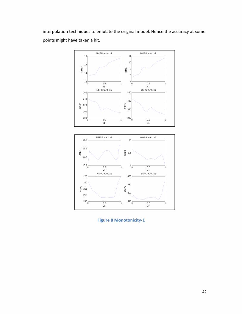
42
interpolation techniques to emulate the original model. Hence the accuracy at some
points might have taken a hit.
Figure 8 Monotonicity‐1
0 0.5 112
14
16
18NMEP w.r.t. x1
x1
NM
EP
0 0.5 17
8
9
10
11BMEP w.r.t. x1
x1
BM
EP
0 0.5 1180
200
220
240
260NSFC w.r.t. x1
x1
NS
FC
0 0.5 1300
350
400
450BSFC w.r.t. x1
x1B
SFC
0 0.5 115.2
15.4
15.6
15.8NMEP w.r.t. x2
x2
NM
EP
0 0.5 19
9.5
10BMEP w.r.t. x2
x2
BM
EP
0 0.5 1205
210
215
220
225NSFC w.r.t. x2
x2
NS
FC
0 0.5 1340
360
380
400BSFC w.r.t. x2
x2
BS
FC

43
Figure 9 Monotonicity‐2
0 0.5 113
14
15
16NMEP w.r.t. x3
x3
NM
EP
0 0.5 17
8
9
10BMEP w.r.t. x3
x3
BM
EP
0 0.5 1200
220
240
260NSFC w.r.t. x3
x3
NS
FC
0 0.5 1300
350
400
450BSFC w.r.t. x3
x3
BS
FC
0 0.5 115
15.5
16
16.5
17NMEP w.r.t. x4
x4
NM
EP
0 0.5 19
9.5
10
10.5BMEP w.r.t. x4
x4
BM
EP
0 0.5 1206
207
208
209
210NSFC w.r.t. x4
x4
NS
FC
0 0.5 1330
335
340
345
350BSFC w.r.t. x4
x4
BS
FC
0 0.5 130
35
40
45ieff w.r.t. x1
x1
ieff
0 0.5 130
35
40
45
50Torque w.r.t. x1
x1
Torq
ue
0 0.5 11
1.5
2
2.5lambda w.r.t. x1
x1
lam
bda
0 0.5 1-160
-150
-140
-130
-120IVC w.r.t. x1
x1
IVC

44
Figure 10 Monotonicity‐3
0 0.5 136
37
38
39
40ieff w.r.t. x2
x2
ieff
0 0.5 137
38
39
40
41Torque w.r.t. x2
x2
Torq
ue
0 0.5 1
1.4
1.6
1.8
2lambda w.r.t. x2
x2
lam
bda
0 0.5 1-160
-150
-140
-130IVC w.r.t. x2
x2
IVC
0 0.5 132
34
36
38
40ieff w.r.t. x3
x3
ieff
0 0.5 130
35
40
45Torque w.r.t. x3
x3
Torq
ue
0 0.5 11
1.5
2
2.5lambda w.r.t. x3
x3
lam
bda
0 0.5 1-180
-160
-140
-120
-100IVC w.r.t. x3
x3
IVC
0 0.5 138.5
39
39.5ieff w.r.t. x4
x4
ieff
0 0.5 138
40
42
44Torque w.r.t. x4
x4
Torq
ue
0 0.5 11.35
1.4
1.45
1.5lambda w.r.t. x4
x4
lam
bda
0 0.5 1-150
-145
-140
-135IVC w.r.t. x4
x4
IVC

45
0 0.5 1504
505
506
507
508T60 w.r.t. x1
x1T6
0
0 0.5 10
50
100RI w.r.t. x1
x1
RI
0 0.5 10
50
100SNOx w.r.t. x1
x1
SN
Ox
0 0.5 10
5
10
15
20CoV w.r.t. x1
x1
CoV
0 0.5 1500
510
520
530T60 w.r.t. x2
x2
T60
0 0.5 10
50
100
150RI w.r.t. x2
x2
RI
0 0.5 10
10
20
30SNOx w.r.t. x2
x2
SN
Ox
0 0.5 10
5
10
15
20CoV w.r.t. x2
x2
CoV
0 0.5 1400
500
600
700
800T60 w.r.t. x3
x3
T60
0 0.5 10
10
20
30RI w.r.t. x3
x3
RI
0 0.5 10
20
40
60SNOx w.r.t. x3
x3
SN
Ox
0 0.5 10
10
20
30
40CoV w.r.t. x3
x3
CoV

46
Figure 11 Monotonicity‐4
From the observation of the variable and constraint dependency the monotonicity
analysis can be performed for the system. The results are presented in Table 7.
x1 x2 x3 x4 f ‐ u ‐ + g1 u + + ‐ g2 ‐ ‐ u u g3 + ‐ ‐ ‐ g4 ‐ u u u g5 + g6 u ‐ + + g7 + g8 ‐ g9 + g10 + ‐ g11 ‐ g12 +
Table 7
+ indicates positive monotonicity
+ indicates negative monotonicity
u indicates that the monotonicity is unknown
Space indicates that the variable does not appear in the constraint
0 0.5 1505.75
505.8
505.85
505.9T60 w.r.t. x4
x4
T60
0 0.5 110.498
10.5
10.502
10.504
10.506RI w.r.t. x4
x4
RI
0 0.5 10
2
4
6SNOx w.r.t. x4
x4
SN
Ox
0 0.5 10
10
20
30
40CoV w.r.t. x4
x4
CoV

47
NOTE: There were some cases where a unidirectional monotonicity is indicated even
though it is not exactly the case. This is owing to the fact that the data was obtained
through interpolation.
The monotonicity analysis is not by any means the ultimate representative of the
system. As can be observed in Table 5, over the entire range of points, there were
points wherein a constraint becomes active and it is not always the case. There were a
few cases where the optimal is in the interior of the design space. Hence a clear analysis
on the monotonicity for the system cannot be performed. The plots in Figure 7 also
illustrate this fact.
Validation:
As the whole optimization run was done based on the surrogate models that were
developed using DoE, there is quite a need to validate the model to check its
genuineness. Hence, for the present study, the model was compared with the original
GT‐Power model to check the emulative ability of the interpolation.
L D P Tin RPM mdotf NMEP BMEP ieff BSFC RI SNOx lambdaGT 0.23 0.91 12.82 328 1000 14 17.48 15.827 38.7 265.34 0.97 4.9203 1.325Est 0.23 0.91 12.82 328 1000 14 18.28 21.532 39.7 173.91 2.03 0.986 1.681GT 0.548 0.848 18.25 348 2000 7 ‐1.583 ‐2.121 ‐7 ‐299 0 0 1.335Est 0.548 0.848 18.25 348 2000 7 11.9 10.618 38.8 231.73 3.55 0.028 1.611GT 0.179 0.948 24.78 343 3000 11 11.6 9.3173 32.7 287.4 15.1 15.097 1.019Est 0.179 0.948 24.78 343 3000 11 13.3 11.189 36.5 264.62 1.75 1.029 1.583GT 0.568 0.972 34.56 323 4000 5.504 ‐1.475 ‐4.715 ‐8.3 ‐980 0 0 1.158Est 0.568 0.972 34.56 323 4000 5.504 10.22 5.651 34.9 425.6 0.52 0.001 1.539
Table 8
The comparison shows that the model is still not good enough to replicate the engine
behavior. The difference is even more evident in the RI and SNOx limits. The model
however does reasonably well with the NMEP prediction. The misfire limits and the RI
limits were not captured properly. This indicates that there is a need to look at more
points to understand the engine better. This can be done as a next step.

48
Additional Work:
1. Simulate the engine at more points to understand the engine better. This will improve
the interpolation capability of the algorithm with more closely knit design space.
2. Because of its limited operational range and start‐up difficulties, a HCCI engine is
generally used in conjunction with an SI engine. The map of the HCCI Engine, hence, is
imposed on the map of the SI engine to increase the operational range of the engine. The
HCCI operational range will be initially investigated and then is superimposed on the SI
engine map to obtain increased operational range. However the present study will not
include the optimization of the SI runs owing to the time constraint.
3. Try out the rebreathing valve strategy for a higher level comparative study between the
valve strategies that can be employed at different loads.
4. Use Optimus/iSight to validate the optimal results that are achieved in the present
study.
5. Try to optimize the ultimate valve strategy employing different strategies at different
load conditions, based on the observations at SAE HCCI symposium[6]

49
Automatic Transmission (Rajit Johri)
Problem Statement
Automatic transmission is one of the most important vehicle level subsystems
influencing the fuel economy. Automatic transmissions are widely used in vehicles to
enable engine to run in a desired range of speeds. The design and tuning of these
automatic transmissions play a crucial role in performance, fuel economy and emissions.
Although parallel hybrids have another power source and engine can be operated with
greater flexibility, automatic transmissions are still required for proper engine
operation.
HCCI engines offer greater fuel economy and better emissions to conventional SI engine
but present design of HCCI engines are limited in their operating range. HCCI
combustion can only be sustained in a narrow band of operating speeds. Commercially
available HCCI engines operate these engines like conventional SI engine outside this
range. With hybrids, because of additional prime mover, engine can be operated in a
narrow range and automatic transmission is the key enabler.
The objective of this subproject is to optimize the conventional five speed automatic
transmission (AT) design to enable HCCI engine to operate in the desired speed band
and hence thereby reducing fuel consumption and emissions but still maintaining
certain performance indices. The project will involve developing models, and optimizing
the design for minimum fuel consumption and emissions.
Dynamic optimization of AT has been carried out previously, Numazawa et al. [10], and
is a well‐studied problem. Traditionally the gear ratios and the shift schedule are
designed from a static analysis and the performance is not optimum in a dynamic
operation. The maps are further tweaked to achieve desired level of operation by
calibration engineers. Jacobson et al. [13] pointed out this deficiency in the AT design
and tried to obtain shift schedule by minimizing a cost function consisting of fuel
consumption & performance criteria (e.g., the acceleration time). Pfeiffer and Haj‐Fraj

50
[11], [12] pursued above approach and applied dynamic programming to discretize gear
shift phase into various stages, and optimized the AT for a cost function consisting of
passenger comfort and performance.
Shift schedules are functions of vehicle‐state parameters, like velocity and throttle, to
select the optimum gear. The goal of this subsystem optimization is to minimize the fuel
consumption while maintaining engine in the desired operating speed band. Overall
vehicle performance indices like acceleration, top speed and towing capacity are
satisfied.
Figure 12: Complex Shift Map
In reality shift schedule are very complex (Figure 12) but to keep the number of
variables and constraints small, a simple shift schedule (Figure 13) with straight lines will
be used. For this optimization, the parameters of the engine, electric motor and vehicle
are fixed. The shift schedule is highly dependent on other subsystems and will be re‐
optimized later with other subsystems to achieve optimal design.

51
Figure 13: Basic Shift Map
Nomenclature
System
MPG Fuel economy (mpg)
Transmission
V12 Vehicle velocity(mph) at 0% throttle during 1‐2 gear up‐shift
V23 Vehicle velocity(mph) at 0% throttle during 2‐3 gear up‐shift
V34 Vehicle velocity(mph) at 0% throttle during 3‐4 gear up‐shift
V45 Vehicle velocity(mph) at 0% throttle during 4‐5 gear up‐shift
V21 Vehicle velocity(mph) at 0% throttle during 2‐1 gear down‐shift

52
V32 Vehicle velocity(mph) at 0% throttle during 3‐2 gear down‐shift
V43 Vehicle velocity(mph) at 0% throttle during 4‐3 gear down‐shift
V54 Vehicle velocity(mph) at 0% throttle during 5‐4 gear down‐shift
A12 Angle extended by 1‐2 gear up‐shift line with x‐axis (deg)
A23 Angle extended by 2‐3 gear up‐shift line with x‐axis (deg)
A34 Angle extended by 3‐4 gear up‐shift line with x‐axis (deg)
A45 Angle extended by 4‐5 gear up‐shift line with x‐axis (deg)
A21 Angle extended by 2‐1 gear down‐shift line with x‐axis (deg)
A32 Angle extended by 3‐2 gear down‐shift line with x‐axis (deg)
A43 Angle extended by 4‐3 gear down‐shift line with x‐axis (deg)
A54 Angle extended by 5‐4 gear down‐shift line with x‐axis (deg)
GR1 1st gear ratio
GR2 2nd gear ratio
GR3 3rd gear ratio
GR4 4th gear ratio
GR5 5th gear ratio
EFFGR Efficiency of Gears
FDR Final drive ratio
Js Propeller shaft inertia (kg/m2)
Ks Propeller shaft stiffness (Nm/rad)

53
Bs Propeller shaft damping (Nm/s/rad)
Engine
N Engine speed (RPM)
tau Engine torque (Nm)
Pe Engine Power (kW)
NEL Minimum engine RPM allowed
NEH Maximum engine RPM allowed
Mathematical Model
1. Objective
Minimize fuel consumption over FUDS cycle
f = Min (–MPG)
MPG = func(V12, V23, V34, V45, A12, A23, A34, A45, V21, V32, V43, V54, A21,
A32, A43, A54, GR1, GR2, GR3, GR4, GR5)
2. Design Variables
The gear ratios are discrete variables (fractions). Nevertheless for this
optimization study the values are assumed to be continuous so as to be able to
apply continuous optimization algorithm. The values returned by the
optimization algorithm need to be then slightly changed to production feasible
gear ratios. Model has following design variables .
Gear ratios – GR1, GR2, GR3, GR4 and GR5
Up Shift variables ‐ V12, V23, V34, V45, A12, A23, A34 and A45

54
Down shift variables – V21, V32, V43, V54, A21, A32, A43 and A54
3. Parameters
Transmission
EFFGR ‐ 0.987
Js ‐ 0.0275 kg/m2
Ks ‐ 14325 Nm/rad
Bs ‐ 46 Nm/s/rad
Engine
NEL ‐ 1000 RPM
NEH ‐ 4000 RPM
4. Constraints
Constraints 1 through 20 are constraints to ensure that the up‐shift and
downshift curves are separated from each other sufficiently and do not cross
each other. Drivability of vehicle depends on these lines closeness. There should
be sufficient gap between up‐shift curve and a corresponding downshift curve to
prevent hysteresis. Closer upshift and downshift lines result in excessive
gearshifts or ’hunting’. Constraints 21 through 36 are the lower and upper
bounds for the variables.
Constraint 37 is to make sure that gears are sorted properly. Constraints 38 to
42 are the lower and upper bounds on the gear ratio. They have been selected
based on experience based on packaging requirements and industry standards.

55
In addition to these constraints, the vehicle must be able to 0‐60 acceleration
timing less than 9 seconds for acceptable performance. It is a non linear implicit
constraint obtained by simulating the model.
V23≥2+V12 (1)
V34≥2+V23 (2)
V45≥2+V34 (3)
‐V12+V21+2≤0 (4)
‐V23+V32+3≤0 (5)
‐V34+V43+4≤0 (6)
‐V45+V54+4≤0 (7)
V21 ‐ 0.85*V12 ≤0 (8)
V32 ‐ 0.85*V23 ≤0 (9)
V21 + 1 ‐ V32 ≤0 (10)
V32 + 1 ‐ V43 ≤0 (11)
V43 + 1 ‐ V54 ≤0 (12)
V34 ‐ 8 ‐ V43 ≤0 (13)
V45 ‐ 8 ‐ V54 ≤0 (14)
(100/tan(A12) + V12) ‐ (100/tan(A23) + V23) ≤0 (15)
(100/tan(A23) + V23) ‐ (100/tan(A34) + V34) ≤0 (16)
(100/tan(A34) + V34) ‐ (100/tan(A45) + V45) ≤0 (17)
(100/tan(A21) + V21) ‐ (100/tan(A32) + V32) ≤0 (18)
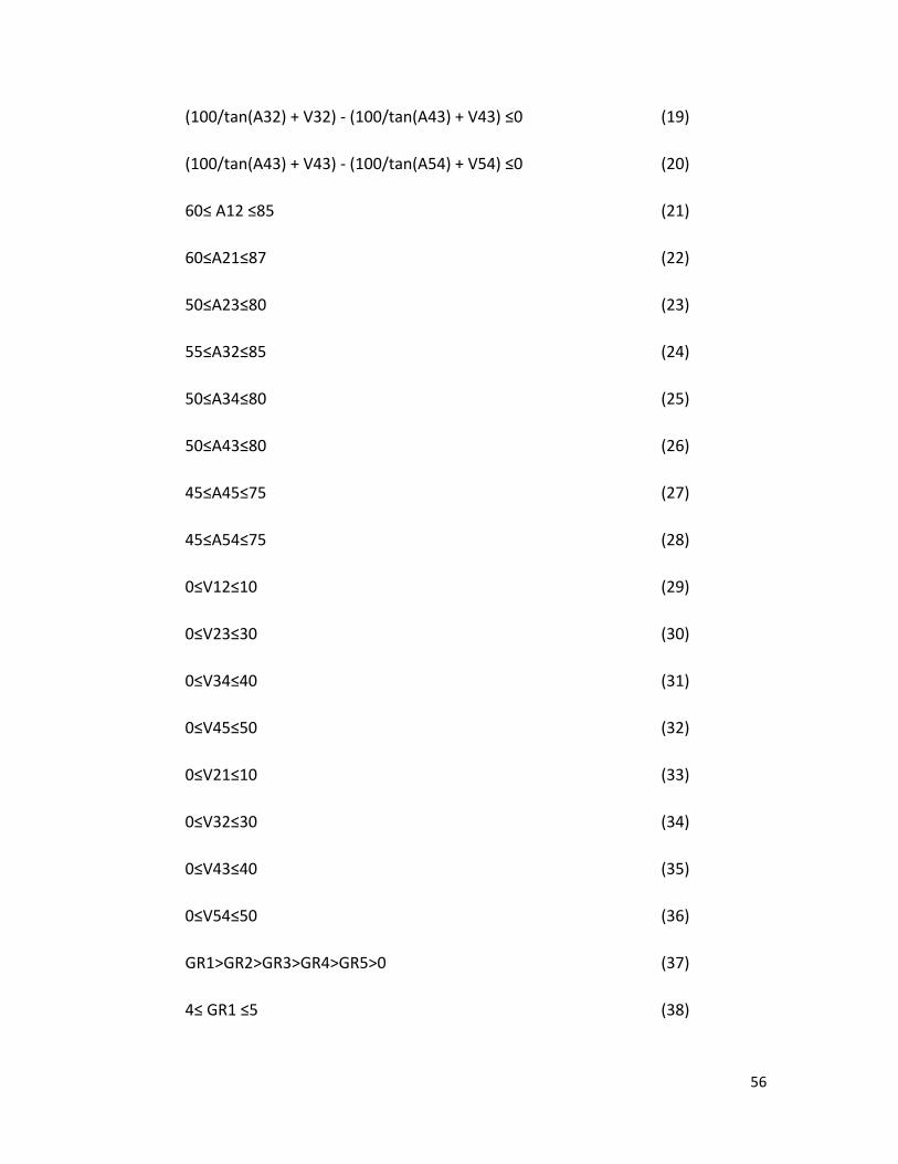
56
(100/tan(A32) + V32) ‐ (100/tan(A43) + V43) ≤0 (19)
(100/tan(A43) + V43) ‐ (100/tan(A54) + V54) ≤0 (20)
60≤ A12 ≤85 (21)
60≤A21≤87 (22)
50≤A23≤80 (23)
55≤A32≤85 (24)
50≤A34≤80 (25)
50≤A43≤80 (26)
45≤A45≤75 (27)
45≤A54≤75 (28)
0≤V12≤10 (29)
0≤V23≤30 (30)
0≤V34≤40 (31)
0≤V45≤50 (32)
0≤V21≤10 (33)
0≤V32≤30 (34)
0≤V43≤40 (35)
0≤V54≤50 (36)
GR1>GR2>GR3>GR4>GR5>0 (37)
4≤ GR1 ≤5 (38)

57
2.6≤GR2≤3.5 (39)
1.5≤GR3≤2.4 (40)
1≤GR4≤1.6 (41)
0.8≤GR5≤1.2 (42)
NEL<N<NEH (43)
5. Simulation Model
To evaluate various designs of AT and shift schedule require simulating the
proposed design candidate with Vehicle engine simulation (Figure 14). The
vehicle level models were used from the Vehicle Engine SIMulation, VESIM
library. High fidelity transmission model was developed to capture the shift
dynamics using simulink/stateflow (Figure 15) and (Figure 16). Also, steady state
engine maps will be used for optimization studies. The aim was to optimize the
design for the vehicle running on Federal Urban Driving Schedule (FUDS) cycle,
which is used by EPA to evaluate fuel economy. Since the optimization problem
was very expensive for complete FUDS cycle, a custom driving cycle, of first 400
seconds was used instead. Also, to evaluate the performance indices like 0‐60
acceleration a custom cycle was developed.

58
Figure 14: Simulation Model (Parallel hybrid electric vehicle)
Figure 15: Simulink model
Figure 16: Stateflow machine
VEHICLE DYNAMICSSimulink based
brake
T wheel _rear
T wheel _front
speed
w wheel
SI ENGINE
load torque
driver demand
engine speed
engine torque
POWER MANAGEMENTParallel
w eng
decel
accel
wheel speed (rad/s)
soc
Power Limit
Brake
engine cmd
motor demand (Nm)
Gain
-K-
Demand Torque (Nm)
motor speed (rad/s)
motor torque (Nm)
net Power
Driving Cycle
Load Input Data
DRIVETRAINParallel
w pump
driver demand
w shaft
motor torque
T pump
T shaft
w prop
DRIVERno preview
configuration 2
speed set
vehicle speed
decel
accel
0
power req'd into bus (W)
SOC
Power limit
impeller torque
vehiclespeed
output torque
T_ratio3
w_ratio2
Gear #1
rad /s --> mph _ref
-K-
Threshold Calculation
run() gear
throttle (%)
down_th
up_th
Shift Logic
speed
up_th
down_th
gear
tsh
CALC_THL
Scope
Blending
Gear
t_shift
w_ratio
T_ratio
-->%
100Throttle
2
w shaft1
gear_state 1fourthentry: gear = 4 ;en:ts h=t*typ ;
fi fthentry: gear = 5 ;en:ts h=t*typ ;
th irdentry: gear = 3 ;en:ts h=t*typ ;
secondentry: gear = 2;en:ts h=t*typ;
fi rstentry: gear = 1;en:ts h=t*typ ;
se lection_stateduring: CALC _TH ;
2
steady_state
upshiftingen:typ =1;
downshiftingen:typ =-1;
UP1
UP UP1
UP1
DOWN
2
DOWN
2DOWN
2DOW N
[speed > up_th & t > abs(ts h)+Ts]1
[speed < down_th & t > abs(ts h)+Ts]2
[speed > down_th]
2
after (TWAIT ,tick)[speed <= down_th]{gear_state.DOWN;}
1after (TWAIT ,tick)[speed >= up_th]{gear_state.UP;}
1
[speed < up_th]
2

59
6. Summary Model
f = Min (–MPG)
subject to
g1 = 2 + V12 ‐ V23 ≤0
g2 = 2 + V23 ‐ V34 ≤0
g3 = 2 + V34 ‐ V45 ≤0
g4 = V21 + 2 ‐ V12 ≤0
g5 = V21 ‐ 0.85*V12 ≤0
g6 = V32 + 3 ‐ V23 ≤0
g7 = V32 ‐ 0.85*V23 ≤0
g8 = V43 + 4 ‐ V34 ≤0
g9 = V54 + 4 ‐ V45 ≤0
g10 = V21 + 1 ‐ V32 ≤0
g11 = V32 + 1 ‐ V43 ≤0
g12 = V43 + 1 ‐ V54 ≤0
g13 = V34 ‐ 8 ‐ V43 ≤0
g14 = V45 ‐ 8 ‐ V54 ≤0
g15 = (100/tan(A12*pi/180) + V12) ‐ (100/tan(A23*pi/180) + V23) ≤0
g16 = (100/tan(A23*pi/180) + V23) ‐ (100/tan(A34*pi/180) + V34) ≤0
g17 = (100/tan(A34*pi/180) + V34) ‐ (100/tan(A45*pi/180) + V45) ≤0

60
g18 = (100/tan(A21*pi/180) + V21) ‐ (100/tan(A32*pi/180) + V32) ≤0
g19 = (100/tan(A32*pi/180) + V32) ‐ (100/tan(A43*pi/180) + V43) ≤0
g20 = (100/tan(A43*pi/180) + V43) ‐ (100/tan(A54*pi/180) + V54) ≤0
g21 = GR2 ‐ GR1 ≤0
g22 = GR3 ‐ GR2 ≤0
g23 = GR4 ‐ GR3 ≤0
g24 = GR5 ‐ GR4 ≤0
Constraints specified in constraint file (MATLAB code) are only specified in the
summary model. Bounds have not been included as they were defined as input
in iSight, optimization software.
Model analysis
1. Scaling
In optimization algorithms, proper scaling is critical when actual design models
are used. For design of automatic transmission problem, design quantities are
expressed in units natural for the problem, e.g. velocity of vehicle are expressed
in miles per hr (mph) with maximum values of order 102, angles of shift lines in
radians with typical values of order 10‐1 rad, while gear ratios are unitless with
magnitude of order 10. Large differences in order of magnitude of variables and
functions (Figure 17) result in ill conditioned Hessian and Jacobian matrices
making algorithmic calculations unstable and inefficient.
For a well‐scaled problem, all variables and functions should have similar
magnitudes in values in the feasible domain and the order of magnitude of
variables in the range [‐1,1]. AT model variables were normalized [‐1,1].

61
Figure 17: Scaling
2. Monotonicity analysis
The model is well bounded, since all the variables have lower and upper bounds.
Most of the constraints are linear making the optimization less expensive. The
objective function is not an explicit function of variables and is obtained by non
linear simulation; therefore any analytical analysis is not possible. But to aid in
monotonicity analysis, the values of one design variable is varied in the feasible
domain, keeping the values of the rest of the variables constant and the change
in the objective is observed.
-6 -4 -2 0 2 4 6-3
-2
-1
0
1
2
3
x
y
ill-scaled problemwell scaled problem (normalized)

62
Figure 18: Fuel Economy (Objective) vs Gear Ratio Monotonicity Analysis
-1 -0.8 -0.6 -0.4 -0.2 0 0.2 0.4 0.6 0.8 123.1
23.2
23.3
Obj
ectiv
e
Normalized Parameter GR1
-1 -0.8 -0.6 -0.4 -0.2 0 0.2 0.4 0.6 0.8 115
20
25
Obj
ectiv
e
Normalized Parameter GR2
-1 -0.8 -0.6 -0.4 -0.2 0 0.2 0.4 0.6 0.8 120
22
24
Obj
ectiv
e
Normalized Parameter GR3
-1 -0.8 -0.6 -0.4 -0.2 0 0.2 0.4 0.6 0.8 122.5
23
23.5
Obj
ectiv
e
Normalized Parameter GR4
-1 -0.8 -0.6 -0.4 -0.2 0 0.2 0.4 0.6 0.8 123
23.2
23.4
Obj
ectiv
e
Normalized Parameter GR5

63
Figure 19: Fuel Economy (Objective) vs Upshift Variables Monotonicity Analysis
-1 -0.5 0 0.5 123.1
23.2
23.3
Obj
ectiv
e
Normalized Parameter V12-1 -0.5 0 0.5 1
15
20
25
Obj
ectiv
e
Normalized Parameter V23
-1 -0.5 0 0.5 120
22
24
Obj
ectiv
e
Normalized Parameter V34-1 -0.5 0 0.5 1
23.1
23.2
23.3
Obj
ectiv
e
Normalized Parameter V45
-1 -0.5 0 0.5 123.1
23.2
23.3
Obj
ectiv
e
Normalized Parameter A12-1 -0.5 0 0.5 1
15
20
25
Obj
ectiv
e
Normalized Parameter A23
-1 -0.5 0 0.5 120
22
24
Obj
ectiv
e
Normalized Parameter A34-1 -0.5 0 0.5 1
23.3
23.4
Obj
ectiv
e
Normalized Parameter A45

64
Figure 20: Fuel Economy (Objective) vs Downshift Variables Monotonicity Analysis
Table 9: Monotonicity Analysis with Gear Ratios
GR1 GR2 GR3 GR4 GR5
f + ~ ~ ‐ ‐
g21 ‐ +
g22 ‐ +
g23 ‐ +
g24 ‐ +
-1 -0.5 0 0.5 122.5
23
23.5
Obj
ectiv
e
Normalized Parameter V21-1 -0.5 0 0.5 1
23
23.2
23.4
Obj
ectiv
e
Normalized Parameter V32
-1 -0.5 0 0.5 122
23
24
Obj
ectiv
e
Normalized Parameter V43-1 -0.5 0 0.5 1
23.3
23.4
Obj
ectiv
e
Normalized Parameter V54
-1 -0.5 0 0.5 120
22
24
Obj
ectiv
e
Normalized Parameter A21-1 -0.5 0 0.5 1
23
23.2
23.4
Obj
ectiv
e
Normalized Parameter A32
-1 -0.5 0 0.5 122
23
24
Obj
ectiv
e
Normalized Parameter A43-1 -0.5 0 0.5 1
23.3
23.4
Obj
ectiv
e
Normalized Parameter A54

65
Table 10: Monotonicity Analysis with Upshift Variables
V12 V23 V34 V45 A12 A23 A34 A45
f ~ + + ~ + ‐ ‐ +
g1 + ‐
g2 + ‐
g3 + ‐
g4 ‐
g5 ‐
g6 ‐
g7 ‐
g8 ‐
g9 ‐
g13 +
g14 +
g15 + ‐ ‐ +
g16 + ‐ ‐ +
g17 + ‐ ‐ +
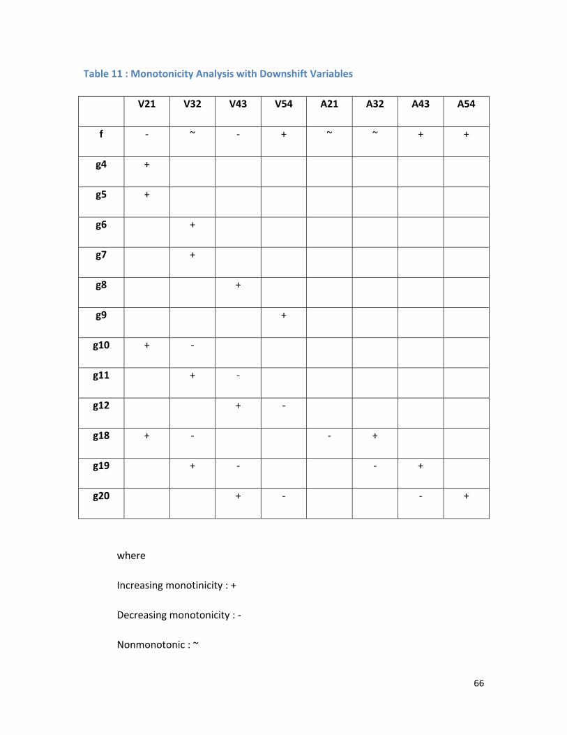
66
Table 11 : Monotonicity Analysis with Downshift Variables
V21 V32 V43 V54 A21 A32 A43 A54
f ‐ ~ ‐ + ~ ~ + +
g4 +
g5 +
g6 +
g7 +
g8 +
g9 +
g10 + ‐
g11 + ‐
g12 + ‐
g18 + ‐ ‐ +
g19 + ‐ ‐ +
g20 + ‐ ‐ +
where
Increasing monotinicity : +
Decreasing monotonicity : ‐
Nonmonotonic : ~
67
It can be seen from monotonicity analysis that the problem is well‐constrained
by Monotonicity Principle 1 (MP1). Every increasing (decreasing) variable in
objective function is bounded below (above) by atleast one active constraint.
3. Optimization Algorithm
Optimization technique adopted for solving AT problem was a two‐step process
as the design search space was large. ASA was used for stage 1 as ASA is well
suited for exploration of large space and the approximate minima was used as
initial guess for stage 2, Non‐Linear Sequential Quadratic Programming (NLSQP)
which converged to local minima.
Adaptive Simulated Annealing (ASA): Simulated annealing (SA) is a generic
probabilistic meta‐algorithm for the global optimization problem, namely
locating a good approximation to the global optimum of a given function in a
large search space. The name and inspiration come from annealing in metallurgy.
In the simulated annealing (SA) method, each point s of the search space is
analogous to a state of some physical system, and the function E(s) to be
minimized is analogous to the internal energy of the system in that state. The
goal is to bring the system, from an arbitrary initial state, to a state with the
minimum possible energy. At each step, the SA heuristic considers some
neighbor s' of the current state s, and probabilistically decides between moving
the system to state s' or staying put in state s. The probabilities are chosen so
that the system ultimately tends to move to states of lower energy. Typically this
step is repeated until the system reaches a state that is good enough for the
application
Adaptive simulated annealing (ASA) is a variant of simulated annealing (SA)
algorithm in which the algorithm parameters that control temperature schedule
and random step selection are automatically adjusted according to algorithm
progress. The algorithm works by representing the parameters of the function to

68
be optimized as continuous numbers, and as dimensions of a hypercube (N
dimensional space).
Non‐Linear Sequential Quadratic Programming (NLSQP) : The sequential
quadratic programming (sequential QP) algorithm is a generalization of Newton's
method for unconstrained optimization in that it finds a step away from the
current point by minimizing a quadratic model of the problem.
4. iSight
iSight [28] is a commercial package for optimization available from Engineous
software. iSight was integrated with MATLAB/SIMULINK for optimization in this
project. All results shown were obtained using iSight.
5. MATLAB (fmincon)
The above problem was also solved using fmincon function available in MATLAB
optimization toolbox [29]. It required larger # of iterations but converged to
similar solution.

69
Figure 21: Optimization Flowchart
Design Concept
Build MATLAB/SIMULINK Model
Adjust Input File(s)Un-Normalize
Run Model
Normalize Resuls
Review Output File(s)
Final Design
MeetRequirements
iSight

70
Results
Total runs = 299
Feasible Runs = 201
Stage 1, ASA runs = 106
Stage 2, NLSQP runs = 193
Lower Bound Initial Guess Upper Bound Stage 1
results (ASA)
Stage 2
results
(NLSQP)
GR1 4 4.68 5 4.75 4.86
GR2 2.6 2.94 3.5 3.22 2.93
GR3 1.5 1.92 2.4 1.64 1.71
GR4 1 1.3 1.6 1.13 1.12
GR5 0.8 1 1.2 0.86 0.88
V12 0 3.44 10 7.75 6.1
V23 0 5.73 30 21.84 25.65
V34 0 17.21 40 33.68 33.61
V45 0 41.31 50 41.82 42.68
V21 0 1 10 1.57 0.83
V32 0 2.73 30 16.44 9.18
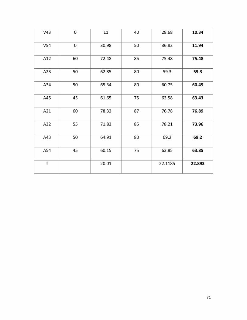
71
V43 0 11 40 28.68 10.34
V54 0 30.98 50 36.82 11.94
A12 60 72.48 85 75.48 75.48
A23 50 62.85 80 59.3 59.3
A34 50 65.34 80 60.75 60.45
A45 45 61.65 75 63.58 63.43
A21 60 78.32 87 76.78 76.89
A32 55 71.83 85 78.21 73.96
A43 50 64.91 80 69.2 69.2
A54 45 60.15 75 63.85 63.85
f 20.01 22.1185 22.893

72
Figure 22: Objective vs RunCounter (Improvements only)
Figure 23: Optimized Shift Map
-25
-20
-15
-10
-5
00 50 100 150 200 250
RunCounter
fmpg
0 10 20 30 40 50 60 70 80 90 1000
10
20
30
40
50
60
70
80
90
100Shift Map
Vehicle Speed (mph)
Thro
ttle
(0 -1
00)
1->22->33->44->52->13->24->35->4

73
Figure 23 is the optimized shift map obtained. Optimization resulted in 14.5%
improvement in fuel economy over initial guess. A better result will be obtained if the
shift map was optimized for complete FUDS cycle.
Table 12: Constraint activity
Constraint Initial Value Final value Activity
g1 ‐0.29 ‐17.54 Inactive
g2 ‐9.48 ‐5.95 Inactive
g3 ‐22.1 ‐7.07 Inactive
g4 ‐0.44 ‐3.27 Inactive
g5 ‐1.924 ‐4.35 Inactive
g6 0 ‐13.46 Inactive
g7 ‐2.14 ‐12.61 Inactive
g8 ‐2.21 ‐0.95 Inactive
g9 ‐6.33 ‐0.622 Inactive
g10 ‐0.73 ‐7.349 Inactive
g11 ‐7.27 ‐18.466 Inactive
g12 ‐18.98 ‐8.407 Inactive
g13 ‐1.79 ‐3.04 Inactive
g14 ‐2.33 ‐3.377 Inactive

74
g15 ‐22.00 ‐53.03 Inactive
g16 ‐6.1076 ‐5.27 Inactive
g17 ‐32.146 ‐2.38 Inactive
g18 ‐13.877 ‐13.82 Inactive
g19 ‐22.271 ‐28.711 Inactive
g20 ‐30.54 ‐20.508 Inactive
g21 ‐1.74 ‐1.929 Inactive
g22 ‐1.02 ‐0.579 Inactive
g23 ‐0.62 ‐0.579 Inactive
g24 ‐0.3 ‐0.248 Inactive
It can be seen from the above table that no constraint is active and hence the solution is
an interior optimum.

75
Structural Analysis of transmission shafts (Girish Chandra)
Problem Statement:
Engine transmission and Power train involve transmission of torque across various
components such as Layshaft, Transmission output shaft, Motor output shaft and the
Propeller shaft. The structural integrity of the connecting shafts is of paramount
importance to ensure safe and reliable vehicle performance.
The connecting shafts experience varying stress states during the performance life cycle
depending on the transmitting torque variation and structural vibration effects.
Understanding the stress distribution caused due to these loading conditions is
necessary to deduce and optimize the structural parameters like shaft inner and outer
diameter.
The objective of this subproject is to perform necessary analytical modeling and carry
out simulations, so as to optimize the shaft structural parameters depending on the
input torque rating. First an analytical model of the stress distribution will be developed
based on beam theory and vibration analysis. The shafts models are analyzed in the FEA
program ANSYS for finding their first few modal frequencies to check for criticalities.
Various simulations are carried out for different loading conditions and shaft
geometries. Finally the integration of this structural analysis component into the project
optimization framework will be discussed. The shafts are designed for steady torque and
fully reversed conditions. because of the absence of an alternating component of
torsional stress, this condition is considered to be a simple multiaxial fatigue case.
There is a trade‐off between the performance and the weight (dimensions) of the shaft
system. Although a thin hollow cylinder results in reduction in the weight of the sub‐
system, a solid cylinder with huge diameter, if considered, could result in infinite
product life time. Our aim is to find an optimum value which could reduce the weight of
the system keeping in performance criteria.
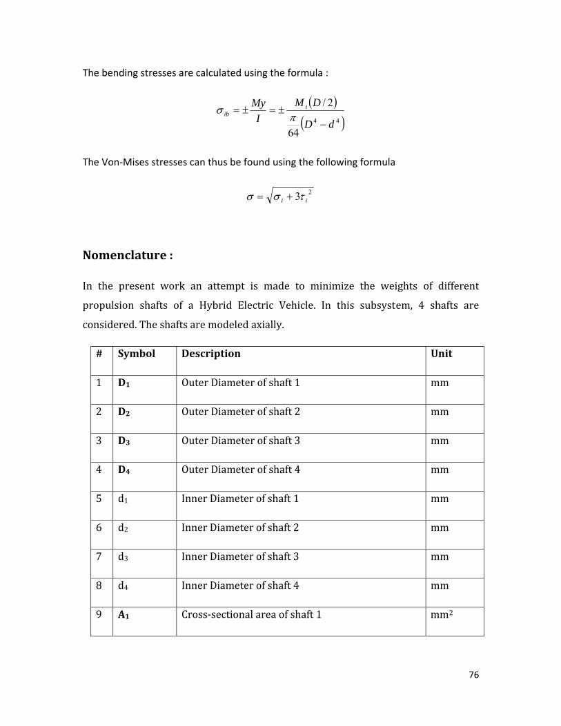
76
The bending stresses are calculated using the formula :
( )( )44
64
2/
dD
DMI
My iib
−±=±=π
σ
The Von‐Mises stresses can thus be found using the following formula
23 ii τσσ +=
Nomenclature :
In the present work an attempt is made to minimize the weights of different
propulsion shafts of a Hybrid Electric Vehicle. In this subsystem, 4 shafts are
considered. The shafts are modeled axially.
# Symbol Description Unit
1 D1 Outer Diameter of shaft 1 mm
2 D2 Outer Diameter of shaft 2 mm
3 D3 Outer Diameter of shaft 3 mm
4 D4 Outer Diameter of shaft 4 mm
5 d1 Inner Diameter of shaft 1 mm
6 d2 Inner Diameter of shaft 2 mm
7 d3 Inner Diameter of shaft 3 mm
8 d4 Inner Diameter of shaft 4 mm
9 A1 Cross‐sectional area of shaft 1 mm2

77
10 A2 Cross‐sectional area of shaft 2 mm2
11 A3 Cross‐sectional area of shaft 3 mm2
12 A4 Cross‐sectional area of shaft 4 mm2
13 σ y Maximum tensile strength N/ mm2
14 Ti Maximum shear stress in shaft i N/ mm2
15 S Maximum Von‐mises stress N/ mm2
16 E Young’s modulus N/ mm2
17 G Shear modulus N/ mm2
18 Nf Factor of safety ‐
19 σ y yield stress N/ mm2
20 Sf Corrected fatigue strength N/ mm2
21 Se Corrected endurance limit N/ mm2
22 Sf’ Fatigue strength N/ mm2
23 Se’ Endurance limit N/ mm2
24 Cload Load factor ‐
26 Csize Size factor ‐
27 Csurf Surface factor ‐
28 Ctemp Temperature factor ‐
29 Creliab Reliability factor ‐
30 Kf Fatigue stress concentration factor (bending) ‐

78
31 Kfs Fatigue stress concentration factor (torsion) ‐
32 Kfsm Mean Torsional Fatigue stress concentration factor ‐
33 Ma Alternating moment N‐m
34 Mm Mean moment N‐m
35 Ta Alternating Torque N‐m
36 Tm Mean Torque N‐m
37 σ a Alternating bending stress N/ mm2
38 σ m Mean bending stress N/ mm2
39 J Mass polar moment of Inertia Kg‐m2
40 Sut Ultimate Strength N/ mm2
Mathematical Model:
Objective
The objective of this optimization process is to minimize consumption of fuel by the
vehicle by minimizing the mass of various shafts involved in the power train. It is
assumed that the shaft rotates at a constant speed about its longitudinal axis, it has a
uniform, circular cross section and is perfectly balanced, i.e., at every cross section, the
mass center coincides with the geometric center.
min w = 2 2( ( - ) )4 iDi di lπ ρ∑
whereDi , di represent the outer and inner diameter of shaft ‘i’ (i = 1, 2, 3, 4)
and il being the corresponding lengths and ρ the density of the material of the shaft.

79
The Transmission output shaft is a splined shaft used to carry the different transmission
gears and transfer the torque as per the selection of the gear by the driver. The stress
concentration factor is selected as per the original shape of the shaft but the varying
diameter of the splines is averaged out as the outer diameter.
An ASME Standard for the Design of Transmission shafting is published as B106.1M‐
1985. This standard presents a simplified approach to the design of shafts. The ASME
approach assumes that the loading is fully reversed bending (zero mean bending
component) and steady torque (zero alternating torque component) at a level that
creates stresses below the torsional yield strength of the material.
Design variables
The objective of minimizing the weight of the 4‐shaft system is achieved considering
varying outer and inner diameters of the shafts. Their lengths are assumed to be
constant and the material properties pre‐selected. The variables of the present
subsystem are :
Inner diameter of the shafts : d1, d2, d3, d4
Outer diameter of the shafts : D1, D2, D3, D4
Parameters
The main parameters of this subsystem are the lengths of the individual shafts (l1, l2, l3,
l4). The 4 shafts are assumed to be made of the same material (cold‐rolled, low‐carbon
steel – SAE 1020). Most of the information on the fatigue strength of a material at some
finite life, or its endurance limit at infinite life, comes from testing of actual or prototype
assemblies of the design. An estimation of the endurance limit and the fatigue strength
of the material is made based on data available from various monotonic tests. From the
various tests, an approximate relationship between Sut and Se’ can be assumed.
Se’ = 0.5* Sut (Sut = 65 Kpsi, Sy = 38 Kpsi)

80
The endurance limit obtained from standard fatigue‐test specimens or from estimates
based on static tests must be modified to account for the physical differences between
the test specimen and the actual part being designed. These factors are accounted as
the strength reduction factors ehich are multiplied directly to the theoretically
estimated values. Thus the endurance limit can be written in the form
Se = Cload* Csize* Csurf* Ctemp* Creliab* Se’ = 0.84* Se’
where Cload, Csize, Csurf, Ctemp, Creliab are the various strength reduction factors as
mentioned above.
The stress concentration factors are very important while considering the design of
shafts. These factors give an indication of degree of stress concentration at a notch. In
the present subsystem, the Transmission output shaft, which is actually a splined shaft,
is assumed to be perfectly cylindrical. The notch sensitivity factor thus plays an
important role in our design and cannot be ignored. For dynamic loading, we need to
modify the theoretical stress‐concentration factor based on the notch sensitivity of the
material to obtain the fatigue stress‐concentration factor, Kf , which can be applied to
the nominal dynamic stresses. Neuber, Kuhn and Peterson developed the concept of
notch‐sensitivity q. the equation for Kf is written as follows
Kf = 1 + q*(Kt ‐ 1) (for Bending)
Kfs = 1 + q*(Kts ‐ 1) (for Torsion)
For most of the design cases, the mean torsional stress component is assumed to be
equal to the torsional fatigue stress concentration factor i.e.
Kfsm = Kfs
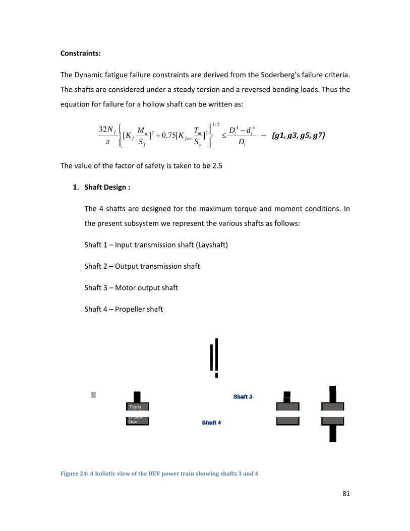
Const
The D
The s
equa
The v
1
Figure
traints:
Dynamic fati
shafts are co
tion for failu
32 fNπ
value of the
1. Shaft Des
The 4 sha
the prese
Shaft 1 –
Shaft 2 –
Shaft 3 –
Shaft 4 –
e 24: A holistic
igue failure c
onsidered un
ure for a hol
2[ ]f af
f
MKS
⎧⎪⎨⎪⎩
factor of saf
sign :
afts are desi
ent subsystem
Input transm
Output tran
Motor outp
Propeller sh
c view of the HE
constraints a
nder a steady
low shaft ca
2 0.75[ fsmK+
fety is taken
igned for th
m we repres
mission shaft
smission sha
ut shaft
haft
EV power train
are derived
y torsion an
n be written
1/ 2
2]m
y
T DS
⎫⎪ ≤⎬⎪⎭
to be 2.5
he maximum
sent the vari
t (Layshaft)
aft
n showing shaf
from the So
d a reversed
n as:
4 4i i
i
D dD− ‐‐
m torque and
ious shafts a
fts 3 and 4
oderberg’s fa
d bending lo
{g1, g3, g5
d moment c
as follows:
8
ailure criteria
ads. Thus th
5, g7}
conditions. I
81
a.
he
In

82
Figure 25: Transmission Gear box containing shafts 1 and 2
For design purposes, the mass of the different gears are assumed to be
independent of the outer/inner diameter of the shafts. Each shaft can thus be
represented by a hollow rotating beam with constant loads acting at different
locations. The locations of the gears are assumed to be fixed. The shafts transmit
their weight through the end bearings which in reality have a certain damping
factor. In the present subsystem we assume the bearings to be free from any
damping effects.
The shafts have been modeled using the mathematical solver MATLAB. The
values of the various components are substituted in the Soderberg’s fatigue
failure criteria, which results in the following equation :
30.57*((5.3127*10^(-9)*M1)^2 + 0.75*(3.81*10^(-9)*T1)^2)^0.5 <= (Di^4-di^4)/Di
We can deduce from the above formula that the constraints g1, g3,g5, g7 are only
dependent on the moments and the torques acting on the shafts (apart from the
inner and outer diameters). Analytical expressions from the Timoshenko’s beam

83
theory and the expressions for loading function using singularity function are
used to calculate the moments acting on the shafts.
The set constraints in the present model are derived from the fact that the
difference in the inner and the outer diameter of the shafts is always negative. To
avoid any singularities in the calculations using MATLAB, we take a factor of
0.001m into consideration. Thus the constraints g2, g4, g6, g8 can be written as
follows
(di+0.001‐Di) ≤ 0
Upper and lower bounds on the both the diameters are placed so as to comply
with the space and various other constraints. Based on past experience, we
limit the maximum outer diameter to 35 cm.
Di – 0.35 ≤ 0
2. Frequency constraints :

84
Figure 26: Campbell Diagram
A Campbell diagram is a mathematically constructed diagram which is used to
check for coincidence of vibration sources with natural resonances. When the
critical speed equals the natural frequency of the shafts, resonance occurs. This
resonance in the structures causes to reduce their product life time. Avoiding
this is one of the most important issues while designing the shaft structures. The
general operating engine speed of a HEV is from 2000 rpm to 5000 rpm. In our
case, we assume this value to be same for the case of Shaft2. Except for this
shaft, all other shafts are found to be well outside this critical range.
The Lay‐shaft is modeled in the Finite Element Analysis package ANSYS for
obtaining its first few modes of vibration under the given loading conditions.
The bearings are assumed to have no damping and are considered to be
completely rigid. The first four modes of vibrations are plotted in the Campbell
0
200
400
600
800
1000
1200
1400
1600
1000 2000 3000 4000 5000 6000
Mode 1
Mode 2
Mode 3
Mode 4
Operating
Critical Speed
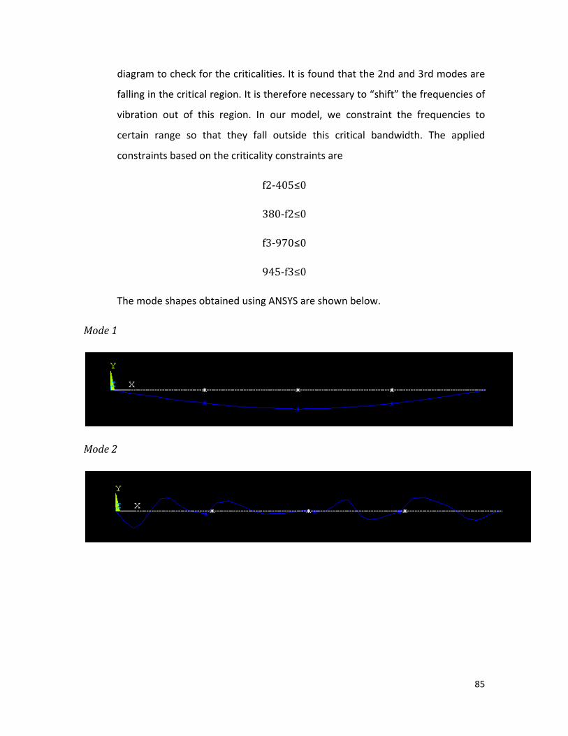
85
diagram to check for the criticalities. It is found that the 2nd and 3rd modes are
falling in the critical region. It is therefore necessary to “shift” the frequencies of
vibration out of this region. In our model, we constraint the frequencies to
certain range so that they fall outside this critical bandwidth. The applied
constraints based on the criticality constraints are
f2‐405≤0
380‐f2≤0
f3‐970≤0
945‐f3≤0
The mode shapes obtained using ANSYS are shown below.
Mode 1
Mode 2
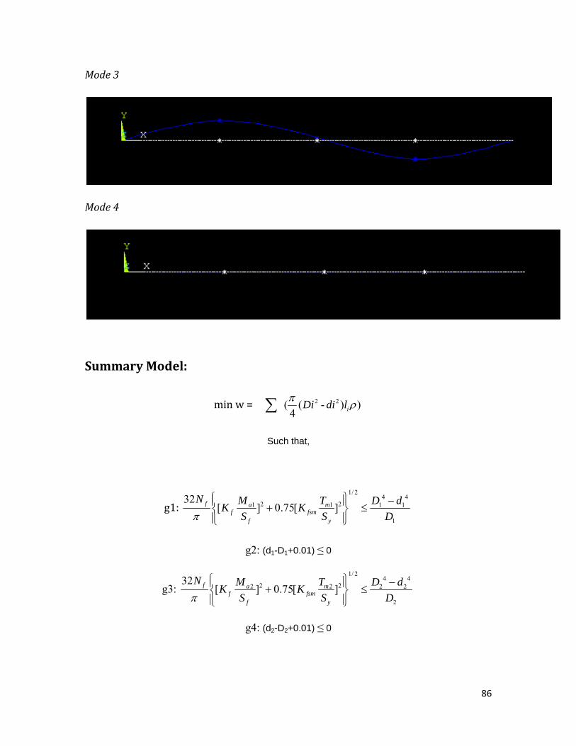
86
Mode 3
Mode 4
Summary Model:
min w = 2 2( ( - ) )4 iDi di lπ ρ∑
Such that,
g1: 1/ 2
4 42 21 1 1 1
1
32[ ] 0.75[ ]f a m
f fsmf y
N M T D dK KS S Dπ
⎧ ⎫ −⎪ ⎪+ ≤⎨ ⎬⎪ ⎪⎩ ⎭
g2: (d1-D1+0.01) ≤ 0
g3: 1/ 2
4 42 22 2 2 2
2
32[ ] 0.75[ ]f a m
f fsmf y
N M T D dK KS S Dπ
⎧ ⎫ −⎪ ⎪+ ≤⎨ ⎬⎪ ⎪⎩ ⎭
g4: (d2-D2+0.01) ≤ 0

87
g5: 1/ 2
4 42 23 3 3 3
3
32[ ] 0.75[ ]f a m
f fsmf y
N M T D dK KS S Dπ
⎧ ⎫ −⎪ ⎪+ ≤⎨ ⎬⎪ ⎪⎩ ⎭
g6: (d3-D3+0.01) ≤ 0
g7: 1/ 2
4 42 24 4 4 4
4
32[ ] 0.75[ ]f a m
f fsmf y
N M T D dK KS S Dπ
⎧ ⎫ −⎪ ⎪+ ≤⎨ ⎬⎪ ⎪⎩ ⎭
g8: (d4-D4+0.01) ≤ 0
g9: D1 ‐ 35 ≤ 0
g10: D2 – 35 ≤ 0
g11: D3 ‐ 35 ≤ 0
g12: D4 ‐ 35 ≤ 0
g13: f2‐405≤0
g14: 380‐f2≤ 0
g15: f3‐970≤ 0
g16: 945‐f3≤ 0
Model validation:
The model was validated by comparing the results of the values obtained using the
formulae derived and used in the MATLAB subroutine with those obtained using
Finite Element Analysis software. For a given di (= .85m) and Di (= 0.12 m), the
values of the moments calculated using the MATLAB file were in congruence with
the ones obtained using FEA software ‐ ANSYS. The initial “guess” values of di=0.09
& Di =0.1 (I = 1 to 4) also were checked for feasibility before the beginning of the
optimization.

88
Model analysis
1. Assumptions:
In the present subsystem, the weight of the transmission gears and the gear
ratios are taken independent of the shaft diameters i.e. they are assumed
constant here. The shafts are assumed to be of constant lengths, small
overhangs (if any) have been ignored. To make the problem less non‐linear, the
power loss due to friction and other factors is ignored. The bearings on which
the shafts are rotating are assumed to be completely stiff, the damping effects
are thus ignored.
2. Monotonicity analysis:
Di (i=1 to 4) di (i=1 to 4) f2 f3
Weight (+) (‐)
Failure constraints (g1 to g4) (‐) (+)
Diameter Set constraints (g5 to g8) (‐) (+) u u
Min. di constraint (‐) u u
Max. di constraint (+) u u
Min. Di constraint (‐) u u
Max. Di constraint (+) u u
Min. 2nd mode freq. (f2) u u (‐)
Max. 2nd mode freq. u u (+)
Min.3rd mode freq. (f3) u u (‐)
Max.3rd mode freq. u u (+)

89
Table 13: Monotonicity analysis on the different variables wrt the constraints and the objective function
The outer diameters are increasing variables with respect to the objective
function. They are bounded below by more than one constraint i.e. we have
more than one active variable with respect (wrt) to the outer diameter(s).
Similarly, the inner diameters of the shafts are decreasing wrt the weight
function and are bounded above by several constraints. The 2nd and 3rd modal
frequencies do not appear in the objective function. Both these frequencies are
bounded both from above and below, thus as per the Monotonicity Principle II,
the problem is well constrained.
The modal frequencies were determined using the Finite Element Analysis code
ANSYS. Their relation with the objective function and other constraints cannot
be exactly determined. Thus their monotonicities are undetermined wrt to the
objective function and the Failure or Diametrical constraints.
The effect of variation of the weight of the shafts with respect to the variation in
the inner and the outer diameter under the different failure and frequency
constraints is analyzed. All the other variables except for the ones specified are
kept constant for this purpose. A contour plot was generated using the least
square regression model and is shown in Figure ‘b’

If a s
value
value
Opti
The
softw
progr
Optim
good
A ma
iterat
value
F
ingle shaft w
e of the oute
es.
imization
optimization
ware iSight.
ramming in
mus with oth
user interfa
aximum sea
tions of 100
es for the o
Figure 27:Effec
was conside
er diameter
n:
n of the 4‐
But later t
Optimus. T
her software
ace was foun
arch length
were consid
uter and inn
ct of variation o
ered, the red
and increas
shaft system
the modelin
This was be
es like ANSY
nd in the latt
of 50, a to
dered for ca
ner diamete
of d1 and D1 o
duction in w
sing the inne
m was first
ng was carr
ecause of th
S. Also, bett
ter software
olerance of
rrying out th
er of all the
on the objectiv
weight is obt
er diameter
carried on
ied out usin
he better in
ter post proc
e.
0.001 and
he optimizat
4 shafts ar
Decreasi
ve function.
tained by de
from the in
using the
ng Sequent
nterfacing ca
cessing capa
a maximum
tion using SQ
re considere
ing
9
ecreasing th
itial specifie
optimizatio
ial Quadrat
apabilities o
abilities and
m number o
QP. The initia
ed same. Th
90
he
ed
on
ic
of
a
of
al
he

91
material of the shafts is also same i.e. cold‐rolled, low‐carbon steel – SAE 1020. This
material is cheap but does not possess very high strength. We thus take a high factor of
safety of 2.5. The material properties (parameters) have already been mentioned in
detail in the previous section. A “.txt” (2nd_shaft.txt) file involving the ANSYS macro was
created. On the execution of this file using a batch file, an output file containing the
results was obtained (s2_results.txt). These files were linked to the corresponding blocks
inside the optimization software Optimus. This work‐flow thus helps in obtaining the
modal frequencies f2 and f3. These frequency values along with the initial diametrical
values are fed into the “.m” file (Opt_HEV.m) which contains the analytical formulae
(steady torsional and reversed bending load), the objective and the constraints.
Execution of this file gives rise to the output “.txt” file (Opt_out.txt). On arranging all
these files as shown in the flow chart below, and on running the iteration process using
SQP, we obtain the optimal solution for the problem.
Figure 28:: Workflow created in Optimus
The results of the optimization are shown below. As we can see constraints g1, g5 and
g8 are only active. None of the 4 frequency constraints are active. We observe that a
decrease in the feasible frequency domain results in an almost same value of the
optimum but an increase in the bounds resulted in the incomplete optimization process

as th
iterat
funct
diam
Futu
In th
assum
damp
and t
e line searc
tions. The in
tion. Results
eters were t
ure Work
he present
med to be
ped bearing
to check for
ch limit was
nitial value o
s could not
taken to be c
subsystem,
completely
g system fo
r their reson
being reach
f the diamet
be obtaine
close to the
Figure 29:
the bearin
stiff. A futu
r the calcul
nance.
hed and Opt
ters was var
ed when the
maximum fe
: Results of Op
ngs on whi
ure work ca
ation of th
timus could
ried to find it
e initial poi
easible value
timus
ch the sha
an be carrie
e modes of
not proces
ts effect on
nt of start
e of D.
fts were ro
ed out by c
f frequency
9
s any furthe
the objectiv
of the oute
otating wer
considering
of the shaf
92
er
ve
er
re
a
ft
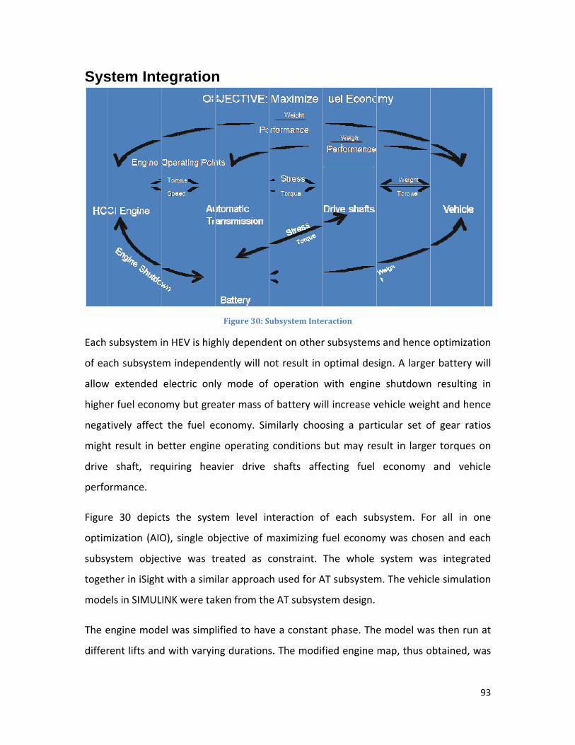
Sys
Each
of ea
allow
highe
negat
migh
drive
perfo
Figur
optim
subsy
toget
mode
The e
differ
stem Inte
subsystem i
ach subsyste
w extended
er fuel econo
tively affect
t result in b
shaft, req
ormance.
e 30 depic
mization (AIO
ystem objec
ther in iSight
els in SIMUL
engine mode
rent lifts and
egration
in HEV is hig
em independ
electric onl
omy but gre
t the fuel e
better engin
quiring hea
cts the syst
O), single ob
ctive was t
t with a simi
LINK were ta
el was simp
d with varyin
n
Figure 30: S
ghly depende
dently will n
ly mode of
eater mass o
conomy. Sim
e operating
avier drive
em level in
bjective of m
reated as c
ilar approac
ken from th
lified to hav
ng durations
ubsystem Inte
ent on other
ot result in
operation
of battery wi
milarly choo
conditions
shafts affe
nteraction o
maximizing f
constraint.
h used for A
e AT subsyst
ve a constan
s. The modif
eraction
r subsystems
optimal des
with engine
ill increase v
osing a part
but may re
ecting fuel
of each sub
fuel econom
The whole
AT subsystem
tem design.
nt phase. The
fied engine
s and hence
sign. A large
e shutdown
vehicle weig
ticular set o
sult in large
economy
bsystem. Fo
my was chos
system wa
m. The vehic
e model wa
map, thus o
9
optimizatio
er battery wi
n resulting i
ht and henc
of gear ratio
er torques o
and vehicl
or all in on
sen and eac
as integrate
cle simulatio
s then run a
obtained, wa
93
on
ill
in
ce
os
on
le
ne
ch
ed
on
at
as

94
used in the engine model. Due to the limited operational range of the HCCI engine, it
was coupled with the base SI engine model and a transition from HCCI to SI and vice‐
versa is made when the operating point crosses the HCCI‐SI map boundary. The system
assumes a very smooth and fast transition between the HCCI and SI modes and the
dynamics of the transition were neglected in the present case. The HCCI engine shows a
much better improvement over the base SI engine in its operational range which
improves the fuel economy of the vehicle.
The structural dynamic subsystem is linked to the other subsystems through the torque
being transmitted across the power train. During the design of the 4‐shaft subsystem, a
constant torque was assumed. Depending upon gear ratios, size of motor and engine,
the maximum torque on shaft changes. Thus, during the integration of the subsystems,
the initially considered structural subsystem parameter (torque) was now a variable.
The optimization of the subsystems involved different objectives. The engine and the
transmission subsystem had maximizing the fuel economy as their objective whereas
the other two subsystems had minimization of the mass as the objective. The system
optimization with AIO was carried out with maximization of fuel economy. Thus the
objectives of the battery and the driveshaft subsystems were incorporated as
intermediate variables affecting the fuel economy through the weight of the vehicle.
Summary Model f = Min (–MPG)
subject to
g1: 2 + V12 ‐ V23 ≤0
g2: 2 + V23 ‐ V34 ≤0
g3: 2 + V34 ‐ V45 ≤0
g4: V21 + 2 ‐ V12 ≤0
g5: V21 ‐ 0.85*V12 ≤0

95
g6: V32 + 3 ‐ V23 ≤0
g7: V32 ‐ 0.85*V23 ≤0
g8: V43 + 4 ‐ V34 ≤0
g9: V54 + 4 ‐ V45 ≤0
g10: V21 + 1 ‐ V32 ≤0
g11: V32 + 1 ‐ V43 ≤0
g12: V43 + 1 ‐ V54 ≤0
g13: V34 ‐ 8 ‐ V43 ≤0
g14: V45 ‐ 8 ‐ V54 ≤0
g15: (100/tan(A12*pi/180) + V12) ‐ (100/tan(A23*pi/180) + V23) ≤0
g16: (100/tan(A23*pi/180) + V23) ‐ (100/tan(A34*pi/180) + V34) ≤0
g17: (100/tan(A34*pi/180) + V34) ‐ (100/tan(A45*pi/180) + V45) ≤0
g18: (100/tan(A21*pi/180) + V21) ‐ (100/tan(A32*pi/180) + V32) ≤0
g19: (100/tan(A32*pi/180) + V32) ‐ (100/tan(A43*pi/180) + V43) ≤0
g20: (100/tan(A43*pi/180) + V43) ‐ (100/tan(A54*pi/180) + V54) ≤0
g21: GR2 ‐ GR1 ≤0
g22: GR3 ‐ GR2 ≤0
g23: GR4 ‐ GR3 ≤0
g24: GR5 ‐ GR4 ≤0
g25: 315.8 0evP n− ≤
g26: 315.8 0rbn P− − ≤
g27: 315.8 0.5 0n a− + ≤
g28: 598.2472 2.25016 0.00675047 30.2269 0evn P s− − + − ≤
g29: 279.4718 0.355285 0.00413003 3.14753 0rn P s− − − − ≤

96
g30: 22.884 1.4031 0.0023136 76.2822 0rn P s− − − + ≤
g31: 0.001299444 0.0000321704 1.90564 7 0.0000734718rn e P+ + − +
g32: 5.56 7 0.0000321704 1.14338 7 0.0000734718 0e n e a s− + − − + ≤
g33: 0.0032 0.000185935 3.13197 7 0.000951056 0en e P s− + − − ≤
g34: 1/ 22 2
4 41 1 1 1
1
320.75 0f a m
f fsmf y
N M T D dK KS S Dπ
⎧ ⎫⎡ ⎤ ⎡ ⎤ −⎪ ⎪+ − ≤⎢ ⎥ ⎢ ⎥⎨ ⎬⎢ ⎥ ⎢ ⎥⎪ ⎪⎣ ⎦ ⎣ ⎦⎩ ⎭
g35: (d1‐D1+0.01) ≤ 0
g36: 1/ 22 2
4 42 2 2 2
2
320.75 0f a m
f fsmf y
N M T D dK KS S Dπ
⎧ ⎫⎡ ⎤ ⎡ ⎤ −⎪ ⎪+ − ≤⎢ ⎥ ⎢ ⎥⎨ ⎬⎢ ⎥ ⎢ ⎥⎪ ⎪⎣ ⎦ ⎣ ⎦⎩ ⎭
g37: (d2‐D2+0.01) ≤ 0
g38: 1/ 22 2
4 43 3 3 3
3
320.75 0f a m
f fsmf y
N M T D dK KS S Dπ
⎧ ⎫⎡ ⎤ ⎡ ⎤ −⎪ ⎪+ − ≤⎢ ⎥ ⎢ ⎥⎨ ⎬⎢ ⎥ ⎢ ⎥⎪ ⎪⎣ ⎦ ⎣ ⎦⎩ ⎭
g39: (d3‐D3+0.01) ≤ 0
g40: 1/ 22 2
4 44 4 4 4
4
320.75 0f a m
f fsmf y
N M T D dK KS S Dπ
⎧ ⎫⎡ ⎤ ⎡ ⎤ −⎪ ⎪+ − ≤⎢ ⎥ ⎢ ⎥⎨ ⎬⎢ ⎥ ⎢ ⎥⎪ ⎪⎣ ⎦ ⎣ ⎦⎩ ⎭
g41: (d4‐D4+0.01) ≤ 0
g42: D1 ‐ 35 ≤ 0
g43: D2 – 35 ≤ 0
g44: D3 ‐ 35 ≤ 0
g45: D4 ‐ 35 ≤ 0
g46: f2‐405≤0

97
g47: 380‐f2≤ 0
g48: f3‐970≤ 0
g49: 945‐f3≤ 0
g50: RI – 4 ≤ 0
g51: SNOx – 1 ≤ 0
g52: CoV ‐ 3 ≤ 0
g53: 1 ‐ Lambda ≤ 0
g54: IVC ‐620 ≤ 0
g55: Tth ‐ T60 ≤ 0
g56: Tin ‐100 ≤ 0
g57: Phmin – Ph ≤ 0
g58: Ph ‐ Phmax ≤ 0
g59: VA ‐ 0.015 ≤ 0
g60: 4 – L ≤ 0
g61: L – 10 ≤ 0
Results
Two different solver, namely, Generalized Reduced Gradient (GRG) and two stage
optimization (ASA followed by SQP), were applied for AIO and
Table 14 gives the summary of final results.
Table 14: AIO results
Lower Initial Upper Two Stage Opt. GRG

98
Bound Guess BoundStage 1 (ASA)
Stage 2 (NLSQP)
GR1 4 4.86 5 4.86 4.9 4.86
GR2 2.6 2.93 3.5 2.93 2.6 3.13
GR3 1.5 1.71 2.4 1.7 1.5 1.69
GR4 1 1.12 1.6 1.13 1.266 1.12
GR5 0.8 0.88 1.2 0.88 1 0.88
V12 0 6.1 10 6.1 4.576 6.1
V23 0 25.65 30 25.65 30 27.68
V34 0 33.61 40 33.61 34.2 35.1
V45 0 42.68 50 42.68 43.96 42.68
V21 0 0.83 10 0.84 0.38 0.83
V32 0 9.18 30 9.18 10.11 9.19
V43 0 10.34 40 10.34 11.37 10.34
V54 0 11.94 50 11.94 13.2 11.94
A12 60 75.48 85 75.48 83.63 75.51
A23 50 59.3 80 59.3 57.27 59.3
A34 50 60.45 80 60.45 59.012 60.45
A45 45 63.43 75 63.44 62.42 63.43
A21 60 76.89 87 76.9 76.9 76.89
A32 55 73.96 85 73.96 73.74 73.96
A43 50 69.2 80 69.2 69.2 69.2
A54 45 63.85 75 63.86 63.85 63.85
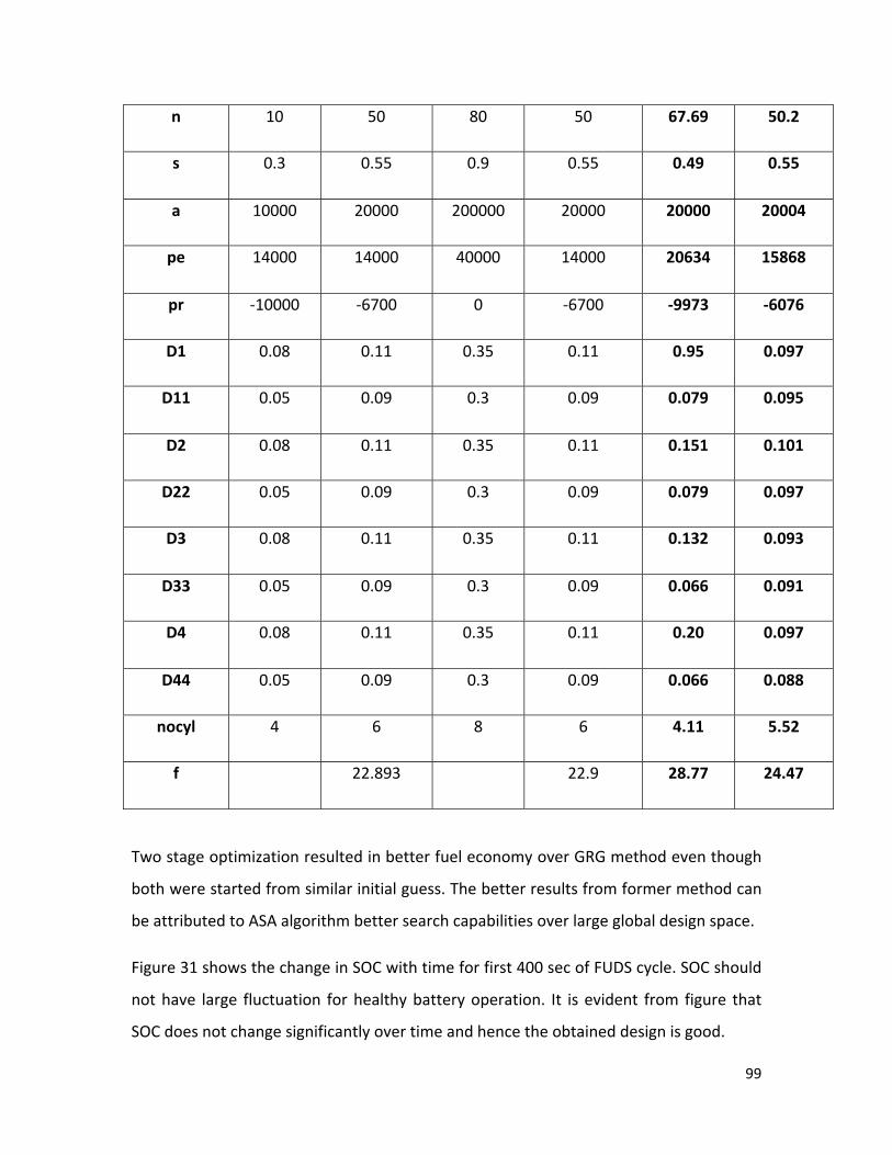
99
n 10 50 80 50 67.69 50.2
s 0.3 0.55 0.9 0.55 0.49 0.55
a 10000 20000 200000 20000 20000 20004
pe 14000 14000 40000 14000 20634 15868
pr ‐10000 ‐6700 0 ‐6700 ‐9973 ‐6076
D1 0.08 0.11 0.35 0.11 0.95 0.097
D11 0.05 0.09 0.3 0.09 0.079 0.095
D2 0.08 0.11 0.35 0.11 0.151 0.101
D22 0.05 0.09 0.3 0.09 0.079 0.097
D3 0.08 0.11 0.35 0.11 0.132 0.093
D33 0.05 0.09 0.3 0.09 0.066 0.091
D4 0.08 0.11 0.35 0.11 0.20 0.097
D44 0.05 0.09 0.3 0.09 0.066 0.088
nocyl 4 6 8 6 4.11 5.52
f 22.893 22.9 28.77 24.47
Two stage optimization resulted in better fuel economy over GRG method even though
both were started from similar initial guess. The better results from former method can
be attributed to ASA algorithm better search capabilities over large global design space.
Figure 31 shows the change in SOC with time for first 400 sec of FUDS cycle. SOC should
not have large fluctuation for healthy battery operation. It is evident from figure that
SOC does not change significantly over time and hence the obtained design is good.

100
Figure 31: SOC evolution with time
Conclusion The use of surrogate models for the engine subsystem reduced effectively the time
taken for the execution. The surrogate models thus are a good trade‐off between time
and fidelity. Whenever a high fidelity is not desired, it is surely advisable to go with a
surrogate model.
The variables for each subsystem (in the individual as well as the system level) are
scaled to make the problem well conditioned. This expedites the convergence of the
model when typical gradient‐based algorithms were used.
Various optimization algorithms have been used to carry out the optimization over the
course of this project. Few of the algorithms used were
• fmincon (MATLAB)
• NLSQP (Non‐linear Sequential Quadratic Programming)
• ASA (Adaptive Simulated Annealing)
• GRG (Generalized Reduced Gradient)
• Linprog (Linear Programming)
0 50 100 150 200 250 300 350 400
0.58
0.585
0.59
0.595
0.6
0.605SOC evolution with time
Time (sec)
SO
C

101
Extensive parametric study was conducted as a part of the optimization study to
understand the sensitivity analysis of the parameters and constraint activity.
Linearization of constraints was done for the battery model to reduce the complexity of
the system. Also the linear nature of the constraint allowed the monotonicity analysis
study easier.
Reference 1. T. Moore, Tools and strategies for hybrid‐electric drivesystem optimization, SAE
paper 961660, SAE, Warrendale, PA, 1996.
2. U Zoelch and D Schroeder, Dynamic optimization method for design and rating
of the components of a hybrid vehicle, International Journal of Vehicle Design
19(1):1‐13 (1998).
3. D Assanis, R Fellini, Z Filipi, Optimization Approach to Hybrid Electric Propulsion
System Design, Mechanics of Structures and Machines, 27(4), 393‐421 (1999).
4. Chan‐Chiao Lin, Jun‐Mo Kang, J.W. Grizzle, and Huei Peng, Energy Management
Strategy for a Parallel Hybrid Electric Truck, Proceedings of the American
Control Conference, Arlington, VA June 25‐27, 2001.
5. R. F. Nelson, "Power requirements for batteries in hybrid electric vehicles,"
Journal of Power Sources, vol. 91, pp. 2‐26, 2000.
6. C. Fellner and J. Newman, "High‐power batteries for use in hybrid vehicles,"
Journal of Power Sources, vol. 85, pp. 229‐236, 2000.
7. J. W. J.‐M. K. Chan‐Chiao Lin; Huei Peng; Grizzle, "Power management strategy
for a parallel hybrid electric truck," Control Systems Technology, IEEE
Transactions on, vol. Volume 11, Issue 6, Nov. 2003 Page(s):839 ‐ 849 2003.

102
8. L. Jinming, P. Huei, and Z. Filipi, "Modeling and Control Analysis of Toyota
Hybrid System," in Advanced Intelligent Mechatronics. Proceedings, 2005
IEEE/ASME International Conference on, 2005, pp. 134‐139.
9. Pfeiffer, F. , Haj‐Fraj, A., Control optimization for automatic transmission, Sixth
International Conference on Motion and Vibration Control. Proceedings, 2002,
879‐84 vol.2.
10. Numazawa, A., Suzuki, K., Yokoi, T., Automatic transmission optimization for
better fuel economy, automatic power transmission, Nov. 1985, 188‐97.
11. Haj‐Fraj, A. Pfeiffer, F., A model based approach for the optimization of
gearshifting in automatic transmissions, International Journal of Vehicle Design,
v 28, n 1‐3, 2002, p 171‐88.
12. Haj‐Fraj, A., Pfeiffer, F., Optimization of gear shift operations in automatic
transmissions, 6th International Workshop on Advanced Motion Control.
Proceedings (Cat. No.00TH8494), 2000, p 469‐73.
13. Jacobson, Bengt , Berglund, Sixten , Optimization of gearbox ratios using
techniques for dynamic systems, Doktorsavhandlingar vid Chalmers Tekniska
Hogskola, n 1468, 1999, 14p.
14. Nebojsa Milovanovic et al, “Influence of the Variable Valve Timing Strategy on
the Control of a Homogeneous Charge Compression (HCCI) Engine", SAE 2004‐
01‐1899, 2004
15. J. L. Chesa Rocafort et al,” A Modeling Investigation into the Optimal Intake and
Exhaust Valve Event Duration and Timing for a Homogenous Charge
Compression Ignition Engine”, SAE 2005‐01‐3746, 2005
16. J. Eng, “Characterization of Pressure Waves in HCCI Combustion”, SAE 2002‐01‐
2859, 2002

103
17. Heywood, J. B.,—“Internal combustion engine fundamentals”—McGraw‐Hill
Book Co., 1988
18. ME 438 course notes
19. Tang Wei Kuo, “Valve and Fueling Strategy for operating a controlled auto‐
ignition combustion engine”, SAE HCCI Symposium, San Ramon CA, Sept 25‐26,
2006
20. Mechanical Engineering Design by Joseph Shigley, Charles Mischke, Richard
Budynas.
21. Optimum design and analysis of composite drive shaft of an automobile –
Gummadi Sanjay and Akula Jagadish Kumar.
22. Principles of Optimal design [Modeling and computation] – Panos. Y.
Papalambrose & Douglas.J.Wilde
23. http://www.diracdelta.co.uk/science/source/c/a/campbell%20diagram/source.h
tml
24. Nick Cristello, and Il Yong Kim : Design optimization of an automotive universal
joint considering manufacturing cost ‐, Mechanical and Materials Engineering,
Queen’s University.
25. The Finite Element Method: Linear Static and Dynamic Finite Element Analysis
by Thomas J. R. Hughes
26. Machine Design by Robert L. Norton
27. Sensitivity Analysis andOptimization of Undamped Rotor Critical Speeds to
Supports stiffness – Shyh‐Chin Huang & Chin‐Ann Lin, National Taiwan University
of Science and Technology
28. iSight v10.0 Manual
29. Matlab R2006a Manual

104
APPENDIX
Battery (Shifang Li)
(1) fmincon
Nonlinear function approximation
The code of the calculation of the gradient and hessian of the nonlinear functions has
been omitted.
clear all; close all; clc
syms n s pe pr
X1 = [n-60 s-0.6 pe-20000]'
X2 = [n-60 s-0.6 pr+5000]'
I10 = 52.7183+X1'*[-1.13237 -0.587409 3.3971e-3]'+(1/2)*X1'*[5.17929e-2
-2.42916e-2 -9.87605e-5; ...
-2.42916e-2 49.3991 7.28748e-5; -9.87605e-5 7.28748e-5 1.26427e-
7]*X1;
I1a = expand(I10);
I1 = simplify(I1a)
I20 = -10.4871+[0.170355 0.344513 2.04426e-3]*X2+(1/2)*X2'*[-5.53823e-3
-2.42916e-2 -3.23878e-5; ...
-2.42916e-2 -2.8191 -6.91885e-5; -3.23878e-5 -6.91885e-5 2.01985e-
8]*X2;
I2a = expand(I20);
I2 = simplify(I20)
V20 = 476.778 +[7.7449 15.6627 -2.41667e-3]*X2+(1/2)*X2'*[-1.6582e-4
0.24673 -1.98985e-6; ...
0.24673 -127.137 -1.71785e-4; -1.98985e-6 -1.71785e-4 -2.38781e-
8]*X2;
V2a = expand(V20);
V2 = simplify(V2a)

105
S10 = -1.62711e-3+[6.2068e-5 1.81299e-5 -1.04849e-7]*X1+(1/2)*X1'*[-
3.66748e-6 4.47576e-7 4.79564e-9;...
4.47576e-7 -1.52466e-3 -2.24922e-9; 4.79564e-9 -2.24922e-9 -
3.90206e-12]*X1;
S1a = expand(S10);
S1 = simplify(S1a)
S20 = 3.23675e-4+[-1.06524e-5 -1.06331e-5 -6.30944e-
8]*X2+(1/2)*X2'*[5.26014e-7 3.55172e-7 2.05119e-9;...
3.55172e-7 8.70093e-5 2.13545e-9; 2.05119e-9 2.13545e-9 -6.2341e-
13]*X2;
S2a = expand(S20);
S2 = simplify(S2a)
Hi1 = [5.17929e-2 -2.42916e-2 -9.87605e-5; ...
-2.42916e-2 49.3991 7.28748e-5; -9.87605e-5 7.28748e-5 1.26427e-7];
ei1 = eig(Hi1)
Hi2 = [-5.53823e-3 -2.42916e-2 -3.23878e-5; ...
-2.42916e-2 -2.8191 -6.91885e-5; -3.23878e-5 -6.91885e-5 2.01985e-
8];
ei2 = eig(Hi2)
Hv2 = [-1.6582e-4 0.24673 -1.98985e-6; ...
0.24673 -127.137 -1.71785e-4; -1.98985e-6 -1.71785e-4 -2.38781e-8];
ev2 = eig(Hv2)
Hs1 = [-3.66748e-6 4.47576e-7 4.79564e-9;...
4.47576e-7 -1.52466e-3 -2.24922e-9; 4.79564e-9 -2.24922e-9 -
3.90206e-12];
es1 = eig(Hs1)
Hs2 = [5.26014e-7 3.55172e-7 2.05119e-9;...
3.55172e-7 8.70093e-5 2.13545e-9; 2.05119e-9 2.13545e-9 -6.2341e-
13];
es2 = eig(Hs2)

106
Main function
clear all; close all;clc
% variables
% n : number of cells %100
% a : SOC P controller gain %2e5
% s : SOC
% pe : EV mode power %4e4
% pr : regenerative braking power %-1e4
% x = [n a s pe pr]
% starting guess
% 100, 2e5, 1, 4e4, -1e4
x0 = [0.2 0.4 0.5 0.5 0.8];
% variable bounds
n_min = 0.1;
a_min = 0.1;
s_min = 0.4;
pe_min = 0.1;
pr_min = 0;
n_max = 1;
a_max = 1;
s_max = 0.7;
pe_max = 1;
pr_max = 1;
lb = [n_min a_min s_min pe_min pr_min]'
ub = [n_max a_max s_max pe_max pr_max]'
% optimization
options = optimset('LargeScale','off','TolX',0.001,'TolFun',0.01,...
'Display','iter','MaxIter',6,'MaxFunEvals',2000);
[x,fval,exitflag,output,lambda,grad,hessian] =
fmincon(@objfun,x0,[],[],[],[],lb,ub,@confun,options);
% display result

107
disp('optimization result');
disp('x: n a s pe pr, f')
disp([x, fval])
msgbox(['num= ',num2str(x(1)),...
' a=',num2str(x(2)),...
' soc=',num2str(x(3)),...
' pe =',num2str(x(4)),...
' pr =',num2str(x(5)),...
' @ f=', num2str(fval)],'Optimization result');
Objective function
function f = objfun(x)
m = 3.6;
gama = 1.08;
f = 100*x(1)*m*gama
Constraint function (1) simplified quadratic form
function [c, ceq] = confun(x)
% Parameters
Ic_min = -291.34;
Id_max = 660.21;
V_max = 9;
Pb_min = 500;
Pc_c_min = -315.8;
Pc_d_max = 315.8;
Cb = 6*60*60/40;
rd_max = 0.002;
rrb_min = 0.0003;
rc_min = 0.001;
% % curve fitting based on experimental data
% Voc = (17.29*(x(3))^5-37.172*(x(3))^4+29.323*(x(3))^3-
10.977*(x(3))^2+2.6624*(x(3))+7.2332);

108
% Rd = (0.01486*(x(3))^4-0.05091*(x(3))^3+0.08153*(x(3))^2-
0.05206*(x(3))+0.03783);
% Rc = (-0.0149*(x(3))^3+0.031987*(x(3))^2-0.020225*(x(3))+0.023541);
%function approximation
Idis = 61.9628 -2.25016*x(1)+0.0258965*x(1)^2+0.00675047*x(4)-
0.0000987605*x(1)*x(4)+...
6.32135e-8*x(4)^2-30.2269*x(3)-
0.0242916*x(1)*x(3)+0.0000728748*x(4)*x(3)+24.6996*x(3)^2;
Ichg_r = -11.8682+0.355285*x(1)-0.00276912*x(1)^2+0.00413003*x(5)-
0.0000323878*x(1)*x(5)+...
1.00993e-8*x(5)^2+3.14753*x(3)-0.0242916*x(1)*x(3)-
0.0000691885*x(5)*x(3)-1.40955*x(3)^2;
Ichg_a = -11.8682+0.355285*x(1)-0.00276912*x(1)^2+0.00413003*(-
0.6*x(2))-0.0000323878*x(1)*(-0.6*x(2))+...
1.00993e-8*(-0.6*x(2))^2+3.14753*x(3)-0.0242916*x(1)*x(3)-
0.0000691885*(-0.6*x(2))*x(3)-1.40955*x(3)^2;
Vchg_r = -22.884+7.59686*x(1)-0.00008291*x(1)^2-0.0023136*x(5)-
1.98985*10-6*x(1)*x(5)-...
1.19391e-8*x(5)^2+76.2822*x(3)+0.24673*x(1)*x(3)-
0.000171785*x(5)*x(3)-63.5685*x(3)^2;
Vchg_a = -22.884+7.59686*x(1)-0.00008291*x(1)^2-0.0023136*(-0.6*x(2))-
1.98985*10-6*x(1)*(-0.6*x(2))-...
1.19391e-8*(-0.6*x(2))^2+76.2822*x(3)+0.24673*x(1)*x(3)-
0.000171785*(-0.6*x(2))*x(3)-63.5685*x(3)^2;
sd_dis = -0.00517751+0.000185935*x(1)-1.83374e-6*x(1)^2-3.13197e-
7*x(4)+4.79564e-9*x(1)*x(4)...
-1.95103e-12*x(4)^2+0.000951056*x(3)+4.47576e-7*x(1)*x(3)-2.24922e-
9*x(4)*x(3)-0.00076233*x(3)^2
sd_chg_r = 0.000999444-0.0000321704*x(1)+2.63007e-7*x(1)^2-1.90564e-
7*x(5)+2.05119e-9*x(1)*x(5)...
109
-3.11705e-13*x(5)^2-0.0000734718*x(3)+3.55172e-
7*x(1)*x(3)+2.13545e-9*x(5)*x(3)+0.0000435047*x(3)^2
sd_chg_a = 0.000999444-0.0000321704*x(1)+2.63007e-7*x(1)^2-1.90564e-
7*(-0.6*x(2))+2.05119e-9*x(1)*(-0.6*x(2))...
-3.11705e-13*(-0.6*x(2))^2-0.0000734718*x(3)+3.55172e-
7*x(1)*x(3)+2.13545e-9*(-0.6*x(2))*x(3)+0.0000435047*x(3)^2
% nonlinear inequality constraints
c(1) = x(4)-x(1)*Pc_d_max; % power limit
c(2) = x(5)-Pb_min;
c(3) = x(1)*Pc_c_min-x(5);
c(4) = x(1)*Pc_c_min-x(2)*(-0.6);
c(5) = Idis-Id_max; % current limit
c(6) = Ic_min -Ichg_a;
c(7) = Ic_min - Ichg_r;
c(8) = Vchg_a-x(1)*V_max; % voltage limit
c(9) = Vchg_r-x(1)*V_max;
c(10) = rrb_min-sd_chg_r; % soc changing rate
c(11) = rc_min-sd_chg_a;
c(12) = -sd_dis-rd_max;
% nonlinear equality constraints
ceq = [];
Constraint function (2) Original constraints
function [c, ceq] = confun(x)
% Parameters
Ic_min = -291.34;
Id_max = 660.21;
V_max = 1.35;
Pb_min = 500;
Pc_c_min = -315.8;
Pc_d_max = 315.8;
Cb = 28*60*60/190;
%----------------------------

110
rd_max = 0.002;
rrb_min = 0.0003;
rc_min = 0.001;
% curve fitting based on experimental data in P-SAT
Voc = (17.29*(x(3))^5-37.172*(x(3))^4+29.323*(x(3))^3-
10.977*(x(3))^2+2.6624*(x(3))+7.2332);
Rd = (0.01486*(x(3))^4-0.05091*(x(3))^3+0.08153*(x(3))^2-
0.05206*(x(3))+0.03783);
Rc = (-0.0149*(x(3))^3+0.031987*(x(3))^2-0.020225*(x(3))+0.023541);
% nonlinear inequality constraints
c(1) = (40000*x(4))-(100*x(1))*Pc_d_max+10; %power limit
c(2) = -Pb_min+(-10000*x(5));
c(3) = (100*x(1))*Pc_c_min-(-10000*x(5));
c(4) = (100*x(1))*Pc_c_min-10000*(200000*x(2))*(-0.6);
c(5) = (Voc*(100*x(1))-sqrt((Voc*(100*x(1)))^2-
4*(Rd*(100*x(1)))*(40000*x(4))))/(2*(Rd*(100*x(1))))-Id_max; % current
limit
c(6) = Ic_min-((Voc*(100*x(1)))-sqrt((Voc*(100*x(1)))^2-
4*(Rc*(100*x(1)))*(-10000*x(5))))/(2*(Rc*(100*x(1))));
c(7) = Ic_min-((Voc*(100*x(1)))-sqrt((Voc*(100*x(1)))^2-
4*(Rc*(100*x(1)))*(200000*x(2))*(-0.6)))/(2*(Rc*(100*x(1))));
c(8) = ((Voc*(100*x(1)))+sqrt((Voc*(100*x(1)))^2-
4*(Rc*(100*x(1)))*(200000*x(2))*(-0.6)))/2-(100*x(1))*V_max; % Voltage
limit
c(9) = ((Voc*(100*x(1)))+sqrt((Voc*(100*x(1)))^2-4*(Rc*(100*x(1)))*(-
10000*x(5))))/2-(100*x(1))*V_max;
c(10) = rrb_min-(sqrt((Voc*(100*x(1)))^2-4*(Rc*(100*x(1)))*(-
10000*x(5)))-(Voc*(100*x(1))))/(2*(Rc*(100*x(1)))*(100*x(1))*Cb); % soc
rate limit
c(11) = -(sqrt((Voc*(100*x(1)))^2-4*(Rd*(100*x(1)))*(40000*x(4)))-
(Voc*(100*x(1))))/(2*(Rd*(100*x(1)))*(100*x(1))*Cb)-rd_max;
c(12) = rc_min-(sqrt((Voc*(100*x(1)))^2-
4*(Rc*(100*x(1)))*(200000*x(2))*(-0.1))-
(Voc*(100*x(1))))/(2*(Rc*(100*x(1)))*(100*x(1))*Cb);
c(13) = -((Voc*(100*x(1)))^2-4*(Rd*(100*x(1)))*(40000*x(4)));% maths
limit

111
c(14) = 0.3-x(3);
% nonlinear equality constraints
ceq = [];
(2) linear programming
clear all;close all; clc
% Linear programming process
% By Taylor expansions to linearize the model
%Objective function
m = 0.9979
gama = 1.08
f=[m*gama 0 0 0 0]';
% linear inequavalent constaints
A = [-315.8 0 0 1 0; ...
-315.8 0 0 0 -1; ...
-315.8 0.6 0 0 0;...
-2.25016 0 -30.2269 6.75047e-3 0;...
-0.355285 0 3.14753 0 -4.13003e-3; ...
-0.355285 0 -30.2269 6.75047e-3 0;...
-0.355285 -4.13003e-3 -3.14753 0 0;...
7.59686-9 0 76.2822 0 -2.3136e-3;...
-1.85935e-4 0 -9.51056e-4 3.13197e-7 0;...
3.21704e-5 0 7.34718e-5 0 1.90564e-7;...
-3.21704e-5 1.90564e-7 0 0 7.34718e-5]
b = [0 0 0 660.21-61.6928 291.34-11.8682 ...
291.34-11.8682 22.884 22.884 0.000717751...
-0.0003+9.99444e-4 -0.001-9.99444e-4]'
% variable bounds
n_min = 0;
a_min = 10000;
s_min = 0.3;
pe_min = 12000;

112
pr_min = -10000;
n_max = 100;
a_max = 200000;
s_max = 0.9;
pe_max = 40000;
pr_max = 0;
lb = [n_min a_min s_min pe_min pr_min]'
ub = [n_max a_max s_max pe_max pr_max]'
% optimization
[x,fval,existflag,output] = linprog(f,A,b,[],[],lb,ub)
% display result
msgbox(['num= ',num2str(x(1)),...
' a=',num2str(x(2)),...
' soc=',num2str(x(3)),...
' pe =',num2str(x(4)),...
' pr =',num2str(x(5)),...
' @ f=', num2str(fval)],...
'Optimization result');

113
HCCI Engine (Prasad Challa) %% Post-processing Routine
clc
clear
for topind = 1:105
dirs{topind} = ['Set-' num2str(topind)];
cd ..
cd(dirs{topind});
dir = [pwd '\']
file1 = ['HCCI_ME555_datafile1.trn'];
file2 = ['HCCI_ME555_datafile2.trn'];
file3 = ['HCCI_ME555_datafile3.trn'];
file4 = ['HCCI_ME555_consol3-01.trn'];
file5 = ['HCCI_ME555_consol4-01.trn'];
file6 = ['HCCIcorrelation.dat'];
file7 = ['NOxdata.dat'];
file8 = ['TPdata.dat'];
SIc = 19;
Trun = 50;
[A1,A2,A3,A4,A5,A6,A7,A8,A9,A10,A11,A12] = textread([dir file1],'%s
%s %s %s %s %s %s %s %s %s %s %s');
casenum = floor(length(A1))/(Trun+6);
arr = [];
for i=1:casenum
arr =[arr 7+(Trun+6)*(i-1):(Trun+6)*i];
end
for ind=1:length(arr)
k = arr(ind);
cycle(ind) = str2double(A1{k});

114
soc(ind) = str2double(A3{k});
b50(ind) = str2double(A4{k});
htav(ind) = str2double(A5{k});
htper(ind) = str2double(A6{k});
pmax(ind) = str2double(A7{k});
pmaxcad(ind) = str2double(A8{k});
dpcyl(ind) = str2double(A9{k});
tmax(ind) = str2double(A10{k});
veff(ind) = str2double(A11{k});
FARtot(ind) = str2double(A12{k});
end
arr = [];
for i=1:casenum
arr =[arr 1+Trun*(i-1):Trun*i-3];
end
cycle = cycle(arr)';
soc = soc(arr+1)';
b50 = b50(arr+1)';
htav = htav(arr+1)';
htper = htper(arr+2)';
pmax = pmax(arr+2)';
pmaxcad = pmaxcad(arr+2)';
dpcyl = dpcyl(arr+2)';
tmax = tmax(arr+2)';
veff = veff(arr+1)';
FARtot = FARtot(arr+1)'; %not sure of this column
clear A1 A2 A3 A4 A5 A6 A7 A8 A9 A10 A11 A12
disp(['Finished first file in the ' num2str(topind) ' set']);
[A1,A2,A3,A4,A5,A6,A7,A8,A9,A10,A11,A12] = textread([dir file2],'%s
%s %s %s %s %s %s %s %s %s %s %s');
arr = [];
for i=1:casenum

115
arr =[arr 6+(Trun+5)*(i-1):(Trun+5)*i];
end
for ind=1:length(arr)
k = arr(ind);
FARtrap(ind) = str2double(A3{k});
airin(ind) = str2double(A4{k});
fuelin(ind) = str2double(A5{k});
fueltrap(ind) = str2double(A6{k});
fuelinj(ind) = str2double(A7{k});
rgf(ind) = str2double(A8{k});
bmep(ind) = str2double(A9{k});
imep(ind) = str2double(A10{k});
imepg(ind) = str2double(A11{k});
fmep(ind) = str2double(A12{k});
end
arr = [];
for i=1:casenum
arr =[arr 1+Trun*(i-1):Trun*i-3];
end
FARtrap = FARtrap(arr+2)';
airin = airin(arr+2)'; %Needs a review
fuelin = fuelin(arr+1)';
fueltrap = fueltrap(arr+1)';
fuelinj = fuelinj(arr+1)';
rgf = rgf(arr)';
bmep = bmep(arr)';
imep = imep(arr)';
imepg = imepg(arr+1)';
fmep = fmep(arr)';
clear A1 A2 A3 A4 A5 A6 A7 A8 A9 A10 A11 A12
disp(['Finished second file in the ' num2str(topind) ' set']);

116
[A1,A2,A3,A4,A5,A6,A7,A8,A9] = textread([dir file3],'%s %s %s %s %s
%s %s %s %s');
arr = [];
for i=1:casenum
arr =[arr 6+(Trun+5)*(i-1):(Trun+5)*i];
end
for ind=1:length(arr)
k = arr(ind);
pmep(ind) = str2double(A3{k});
beff(ind) = str2double(A4{k});
ieff(ind) = str2double(A5{k});
bsfc(ind) = str2double(A6{k});
veffeng(ind) = str2double(A7{k});
nvo(ind) = str2double(A8{k});
ivc(ind) = str2double(A9{k});
end
arr = [];
for i=1:casenum
arr =[arr 1+Trun*(i-1):Trun*i-3];
end
pmep = pmep(arr+2)';
beff = beff(arr+1)';
ieff = ieff(arr+1)';
bsfc = bsfc(arr+1)';
veffeng = veffeng(arr+1)';
nvo = nvo(arr)';
ivc = ivc(arr)';
clear A1 A2 A3 A4 A5 A6 A7 A8 A9
disp(['Finished third file in the ' num2str(topind) ' set']);
[A1,A2,A3,A4,A5,A6,A7] = textread([dir file4],'%s %s %s %s %s %s
%s');

117
arr = [];
for i=1:casenum
arr =[arr 5+(Trun+4)*(i-1):(Trun+4)*i];
end
for ind=1:length(arr)
k = arr(ind);
Btrq1(ind) = str2double(A3{k});
BMEP1(ind) = str2double(A4{k});
BSFC1(ind) = str2double(A5{k});
lambda1(ind) = str2double(A6{k});
ivc1(ind) = str2double(A7{k});
end
arr = [];
for i=1:casenum
arr =[arr 1+Trun*(i-1):Trun*i-3];
end
Btrq1 = Btrq1(arr)';
BMEP1 = BMEP1(arr)'; %Needs a review
BSFC1 = BSFC1(arr+1)';
lambda1 = lambda1(arr+1)';
ivc1 = ivc1(arr)';
clear A1 A2 A3 A4 A5 A6 A7
disp(['Finished fourth file in the ' num2str(topind) ' set']);
[A1,A2,A3,A4,A5,A6,A7,A8,A9,A10] = textread([dir file5],'%s %s %s
%s %s %s %s %s %s %s');
arr = [];
for i=1:casenum
arr =[arr 6+(Trun+5)*(i-1):(Trun+5)*i];
end

118
for ind=1:length(arr)
k = arr(ind);
RPM1(ind) = str2double(A3{k});
Temp1(ind) = str2double(A4{k});
Phase1(ind) = str2double(A5{k});
Liftm1(ind) = str2double(A6{k});
Angm1(ind) = str2double(A7{k});
mfdot1(ind) = str2double(A8{k});
Tin1(ind) = str2double(A9{k});
LbyAAM1(ind) = str2double(A10{k});
end
arr = [];
for i=1:casenum
arr =[arr 1+Trun*(i-1):Trun*i-3];
end
RPM1 = RPM1(arr)';
Temp1 = Temp1(arr)'; %Needs a review
Phase1 = Phase1(arr)';
Liftm1 = Liftm1(arr)';
Angm1 = Angm1(arr)';
mfdot1 = mfdot1(arr)';
Tin1 = Tin1(arr)';
LbyAAM1 = LbyAAM1(arr)';
clear A1 A2 A3 A4 A5 A6 A7 A8 A9 A10
disp(['Finished fifth file in the ' num2str(topind) ' set']);
[A1,A2,A3,A4,phipr,AFR,
rgf_1,soc_1,b50_1,b90,ceff,ceff_GT,tmax_1,bdu,ww,tivc,ttdc,T60] =
textread([dir file6],...
'%f %f %f %f %f %f %f %f %f %f %f %f %f %f %f %f %f %f');
siarr = [];
hcciarr = [];
for i=1:casenum
siarr =[siarr 1+Trun*(i-1):SIc+Trun*(i-1)];

119
hcciarr = [hcciarr SIc+1+Trun*(i-1):Trun*i-3];
end
soc_1(siarr) = A2(siarr);
%
% tivc = zeros(size(A1));
% ttdc = zeros(size(A1));
tivc(siarr) = A3(siarr);
ttdc(siarr) = A4(siarr);
ceff(siarr) = 0.98;
ceff_GT(siarr) = 0.98;
clear A1 A2 A3 A4
arr = [];
arr1 = [];
for i=1:casenum
arr = [arr 1+Trun*(i-1):Trun*i-3];
end
phipr = phipr(arr);
AFR = AFR(arr);
rgf_1 = rgf_1(arr);
soc_1 = soc_1(arr);
b50_1 = b50_1(arr);
b90 = b90(arr);
ceff = ceff(arr);
ceff_GT = ceff_GT(arr);
tmax_1 = tmax_1(arr);
bdu = bdu(arr);
ww = ww(arr);
tivc = tivc(arr);
ttdc = ttdc(arr);
T60 = T60(arr);
disp(['Finished sixth file in the ' num2str(topind) ' set']);
120
[A1,A2,A3] = textread([dir file7],'%f %f %f');
hcciarr = [];
for i=1:casenum
hcciarr = [hcciarr SIc+1+Trun*(i-1):Trun*i];
end
tvar1 = find(A1==50);
tvar2 = tvar1(2:end) - tvar1(1:end-1);
tempvar3 = tvar1(find(tvar2<31));
tvar4 = A1(1:31);
if tvar4(end)~=50
A3(2:end+1) = A3(1:end);
end
for index = 1:length(tempvar3)
tempvar4 = tempvar3(index);
A3(tempvar4) = 0;
A3(tempvar4+1:end+1) = A3(tempvar4:end);
end
SNOx = zeros(casenum*Trun,1);
SNOx(hcciarr) = A3;
SNOx = SNOx(arr);
clear A1 A2 A3
disp(['Finished seventh file in the ' num2str(topind) ' set']);
[A1,A2,A3,A4,A5,A6,A7,A8,A9] = textread([dir file8],'%f %f %f %f %f
%f %f %f %f');
tvar1 = find(A1==50);
tvar2 = tvar1(2:end) - tvar1(1:end-1);
tempvar3 = tvar1(find(tvar2<31));
tvar4 = A1(1:31);

121
if tvar4(end)~=50
A9(2:end+1) = A9(1:end);
end
for index = 1:length(tempvar3)
tempvar4 = tempvar3(index);
A9(tempvar4) = 0;
A9(tempvar4+1:end+1) = A9(tempvar4:end);
end
A9 = [A9; A9(end)*ones((6200-length(A9)),1)];
Rind = zeros(casenum*Trun,1);
Rind(hcciarr) = A9;
Rind = Rind(arr);
clear A1 A2 A3 A4 A5 A6 A7 A8 A9
disp(['Finished eigth file in the ' num2str(topind) ' set']);
cd ..
cd('Matlab Files');
Trun = 50; Tcase = Trun - 3; icycle = 19;
ic = icycle:Tcase:length(cycle);
ic_end = Tcase:Tcase:length(cycle);
for ind = 1:length(ic_end)
ic_end_dup(4*ind-3:4*ind) = [ic(ind) ic(ind)+1 ic_end(ind)-1
ic_end(ind)];
end
ic_end = ic_end_dup;
isfc = bsfc.*bmep./imep;

122
data1 = [fuelinj cycle RPM1 Liftm1 Angm1 Phase1 Tin1 Btrq1 BMEP1
BSFC1 lambda1 ivc1 soc b50 imep b90 htav htper pmax pmaxcad dpcyl
Rind/10^6 tmax ...
SNOx veff FARtot FARtrap airin fuelin fueltrap rgf bmep imepg
fmep pmep beff ieff bsfc isfc veffeng ivc phipr AFR AFR/14.7 ceff
ceff_GT bdu ...
ww tivc ttdc T60 tmax_1];
if topind>1
data = textread('NVOdata.txt');
data = data(:,1:52);
else
data=[];
end
data = [data; data1(ic_end,:)];
fid = fopen('NVOdata.txt','wt');
for in=1:size(data,1)
fprintf(fid,'%6.3f\t',data(in,:));
fprintf(fid,'\n');
end
fclose(fid)
fid = fopen('indcount.txt','wt');
fprintf(fid,'%f',topind);
fprintf(fid,'\n');
fclose(fid);
clear
topind = textread('indcount.txt');
topind = topind+1;
end
Trun = 50; Tcase = Trun - 3; icycle = 19; CoVlim = 0.03; SNOxlim = 1;
RIlim = 4;

123
data = textread('NVOdata.txt');
data = data(:,1:52);
title1 = {'fuelinj' 'cycle' 'RPM' 'LIFTM' 'ANGM' 'PHASE' 'Tin' 'Torque'
'BMEP' 'BSFC' 'Lambda' 'IVC' 'SOC' 'CA50' 'NMEP' 'CA90(deg)' 'htav'
'htper' 'pmax' 'pmaxcad' 'dpcyl' 'Ring Ind' 'Tmax' ...
'SNOx' 'veff' 'FARtot' 'FARtrap' 'airin' 'fuelin' 'fueltrap' 'rgf'
'bmep' 'imepg' 'fmep' 'pmep' 'beff' 'ieff' 'bsfc' 'isfc' 'veffeng'
'ivc' 'phipr' 'AFR' 'l' 'ceff' 'ceff_GT' 'BurnDur' ...
'WW' 'TIVC' 'TTDC' 'T60' 'Tmax_corr'};
fid = fopen('NVOdata.txt','wt');
fprintf(fid,'%s\t',title1{1:end});
fprintf(fid,'\n');
for i=1:size(data,1)
fprintf(fid,'%6.3f\t',data(i,:));
fprintf(fid,'\n');
end
fclose(fid)
%% Data Extraction Routine
clear
clc
title1 = {'cycle' 'LIFTM' 'ANGM' 'PHASE' 'Tin' 'RPM'
'fuelinj' 'Torque' 'BMEP' 'BSFC' 'Lambda' 'IVC'
'SOC' 'CA50' 'NMEP' 'CA90(deg)' 'htav' 'htper'
'pmax' 'pmaxcad' 'dpcyl' 'Ring Ind' 'Tmax'
'SNOx' 'veff' 'FARtot' 'FARtrap' 'airin'
'fuelin' 'fueltrap' 'rgf' 'bmep' 'imepg' 'fmep'
'pmep' 'beff' 'ieff' 'bsfc' 'isfc'
'veffeng' 'ivc' 'phipr' 'AFR' 'l' 'ceff' 'ceff_GT'
'BurnDur' 'WW' 'TIVC' 'TTDC' 'T60' 'Tmax_corr'};
data = xlsread('ME555_Valid_Data.xls');
len = size(data,1);
len1 = size(data1,1);

124
len2 = size(data2,1);
dim = 6;
x1 = data(1:len,2); % LIFTM
x2 = data(1:len,3); % ANGM
x3 = data(1:len,4); % PHASE
x4 = data(1:len,5); % Tin
x5 = data(1:len,6); % RPM
x6 = data(1:len,7); % mdotf
x11 = data1(1:len1,1); % LIFTM
x21 = data1(1:len1,2); % ANGM
x31 = data1(1:len1,3); % PHASE
x41 = data1(1:len1,4); % Tin
x51 = data1(1:len1,5); % RPM
x61 = data1(1:len1,6); % mdotf
x12 = data2(1:len2,1); % LIFTM
x22 = data2(1:len2,2); % ANGM
x32 = data2(1:len2,3); % PHASE
x42 = data2(1:len2,4); % Tin
x52 = data2(1:len2,5); % RPM
x62 = data2(1:len2,6); % mdotf
NMEP = data(1:len,15);
BMEP = data(1:len,9);
torq = data(1:len,8);
BSFC = data(1:len,10);
NSFC = data(1:len,39);
Ceff = data(1:len,45);
ieffnet = data(1:len,37);
beff = data(1:len,36);
RI = data(1:len,22);
SNOx = data(1:len,24);
lambda = data(1:len,44);
IVC = data(1:len,41);

125
CoV = data1(1:len1,7);
T60 = data2(1:len2,7);
Optimal_map;
%% Data Interpolation Routine
yr = [NMEP BMEP torq NSFC BSFC Ceff ieffnet beff lambda SNOx IVC RI];
xr = [x1 x2 x3 x4 x5 x6]';
yr1 = CoV;
yr2 = T60;
xr1 = [x11 x21 x31 x41 x51 x61]';
xr2 = [x12 x22 x32 x42 x52 x62]';
x = [0.5 0.5 1 0 0 0];
title2 = {'NMEP' 'BMEP' 'torq' 'NSFC' 'BSFC' 'Ceff' 'ieffnet' 'beff'
'Lambda' 'SNOx' 'IVC' 'RI'};
for i = 1:size(yr,2)
y1(i) = mlliblip('Value',dim,len,x,xr,yr(:,i),2);
LC(i) = mlliblip('ComputeLipschitz',dim,len,xr,yr(:,i));
y2(i) = mlliblip('Value',dim,len,x,xr,yr(:,i),LC(i));
end
y11 = mlliblip('Value',dim,len1,x,xr1,yr1,2);
LC1 = mlliblip('ComputeLipschitz',dim,len1,xr1,yr1);
y21 = mlliblip('Value',dim,len1,x,xr1,yr1,LC1);
y12 = mlliblip('Value',dim,len2,x,xr2,yr2,2);
LC2 = mlliblip('ComputeLipschitz',dim,len2,xr2,yr2);
y22 = mlliblip('Value',dim,len2,x,xr2,yr2,LC2);
find_opt;
%% Finding Optimal points over the entire Engine map
%% Normalization Data
RPMmin = 1000; RPMmax = 5000;
mfdotmin = 7; mfdotmax = 18;
126
Lmin = 0.077; Lmax = 1.1;
Dmin = 0.526; Dmax = 1;
Pmin = -68.726; Pmax = 40;
Timin = 323.15; Timax = 373.15;
RImin = 0; RImax = 1564.3;
SNmin = 0; SNmax = 175.82;
BMmin = -2.63; BMmax = 27.9195;
Tmin = -17.2485; Tmax = 122.0865;
NMmin = 5.46; NMmax = 24.064;
lamin = 2.202; lamax = 1.001;
iemin = 23.729; iemax = 41.869;
bemin = -11.496; bemax = 32.814;
Tcmin = 608.84; Tcmax = 829.9;
NSmin = 194.093; NSmax = 342.467;
Comin = 0; Comax = 71.06732;
RPM = [4000:250:5000];
mfdot = [4:0.5:8 9:13 13.5:0.5:20];
x5v = (RPM-RPMmin)/(RPMmax-RPMmin);
x6v = (mfdot-mfdotmin)/(mfdotmax-mfdotmin);
xopt = [];yfin = [];
[x1,x2,x3,x4]=ndgrid([0.1:0.1:1],[0.1:0.1:1],[0:0.1:1],[0:0.1:1]);
x1 = reshape(x1,prod(size(x1)),1);
x2 = reshape(x2,prod(size(x2)),1);
x3 = reshape(x3,prod(size(x3)),1);
x4 = reshape(x4,prod(size(x4)),1);
for i = 1:length(x5v)
for j = 1:length(x6v)
tic
x5 = x5v(i)*ones(size(x1));
x6 = x6v(j)*ones(size(x1));
for ki = 1:size(x1)
x = [x1(ki) x2(ki) x3(ki) x4(ki) x5(ki) x6(ki)];
for k = 1:size(yr,2)

127
yval(ki,k) =
mlliblip('Value',dim,len,x,xr,yr(:,k),LC(k));
end
yval(ki,size(yr,2)+1) =
mlliblip('Value',dim,len1,x,xr1,yr1,LC1);
yval(ki,size(yr,2)+2) =
mlliblip('Value',dim,len2,x,xr2,yr2,LC2);
end
RIv = (RImax-RImin)*yval(:,12)+RImin;
SNOxv = (SNmax-SNmin)*yval(:,10)+SNmin;
lambdav = (lamax-lamin)*yval(:,9)+lamin;
NMEPv = (NMmax-NMmin)*yval(:,1)+NMmin;
BMEPv = (BMmax-BMmin)*yval(:,2)+BMmin;
ieffv = (iemax-iemin)*yval(:,7)+iemin;
beffv = (bemax-bemin)*yval(:,8)+bemin;
Torqv = (Tmax-Tmin)*yval(:,3)+Tmin;
NSFCv = (NSmax-NSmin)*yval(:,4)+NSmin;
BSFCv = NSFCv.*NMEPv./BMEPv;
T60v = (Tcmax-Tcmin)*yval(:,14)+Tcmin;
Covv = (Comax-Comin)*yval(:,13)+Comin;
RPMv = (RPMmax-RPMmin)*x5+RPMmin;
mfdotv = (mfdotmax-mfdotmin)*x6+mfdotmin;
Tthv = 570 + 25*RPMv/1000;
%% Brake Parameter Positivity
BSFCv = (BSFCv+abs(BSFCv))/2;
beffv = (beffv+abs(beffv))/2;
BMEPv = (BMEPv+abs(BMEPv))/2;
Torqv = (Torqv+abs(Torqv))/2;
y = [x1 x2 x3 x4 x5 x6 NMEPv BMEPv ieffv BSFCv Torqv RIv SNOxv
lambdav T60v Tthv Covv];
i1 = find(y(:,14)>=0.98);
y = y(i1,:);
i2 = find(y(:,12)<=4.2);
y = y(i2,:);
i3 = find(y(:,13)<=1.05);

128
y = y(i3,:);
i4 = find(y(:,15)>=y(:,16));
y = y(i4,:);
i5 = find(y(:,1)<=y(:,2).^2);
y = y(i5,:);
i6 = find(y(:,end)<=3.2);
y = y(i6,:);
[tmp,i7] = max(y(:,7));
if i7~=0
yf = y(i7(1),:);
else
yf = zeros(1,17);
end
[x1m,x2m,x3m,x4m]=ndgrid([max(yf(1)-
0.1,0.1):0.01:min(yf(1)+0.1,1)],[max(0.1,yf(2)-
0.1):0.01:min(yf(2)+0.1,1)],[max(yf(3)-
0.1,0):0.01:min(yf(3)+0.1,1)],yf(4));
x1m = reshape(x1m,prod(size(x1m)),1);
x2m = reshape(x2m,prod(size(x2m)),1);
x3m = reshape(x3m,prod(size(x3m)),1);
x4m = reshape(x4m,prod(size(x4m)),1);
x5m = x5v(i)*ones(size(x1m));
x6m = x6v(j)*ones(size(x1m));
yval = [];
for ki = 1:size(x1m)
x = [x1m(ki) x2m(ki) x3m(ki) x4m(ki) x5m(ki) x6m(ki)];
for k = 1:size(yr,2)
yval(ki,k) =
mlliblip('Value',dim,len,x,xr,yr(:,k),LC(k));
end
yval(ki,size(yr,2)+1) =
mlliblip('Value',dim,len1,x,xr1,yr1,LC1);
yval(ki,size(yr,2)+2) =
mlliblip('Value',dim,len2,x,xr2,yr2,LC2);
end

129
RIv = (RImax-RImin)*yval(:,12)+RImin;
SNOxv = (SNmax-SNmin)*yval(:,10)+SNmin;
lambdav = (lamax-lamin)*yval(:,9)+lamin;
NMEPv = (NMmax-NMmin)*yval(:,1)+NMmin;
BMEPv = (BMmax-BMmin)*yval(:,2)+BMmin;
ieffv = (iemax-iemin)*yval(:,7)+iemin;
beffv = (bemax-bemin)*yval(:,8)+bemin;
Torqv = (Tmax-Tmin)*yval(:,3)+Tmin;
NSFCv = (NSmax-NSmin)*yval(:,4)+NSmin;
BSFCv = NSFCv.*NMEPv./BMEPv;
T60v = (Tcmax-Tcmin)*yval(:,14)+Tcmin;
Covv = (Comax-Comin)*yval(:,13)+Comin;
RPMv = (RPMmax-RPMmin)*x5m+RPMmin;
mfdotv = (mfdotmax-mfdotmin)*x6m+mfdotmin;
Tthv = 570 + 25*RPMv/1000;
%% Brake Parameter Positivity
BSFCv = (BSFCv+abs(BSFCv))/2;
beffv = (beffv+abs(beffv))/2;
BMEPv = (BMEPv+abs(BMEPv))/2;
Torqv = (Torqv+abs(Torqv))/2;
y = [x1m x2m x3m x4m x5m x6m NMEPv BMEPv ieffv BSFCv Torqv RIv
SNOxv lambdav T60v Tthv Covv];
i1 = find(y(:,14)>=0.98);
y = y(i1,:);
i2 = find(y(:,12)<=4.2);
y = y(i2,:);
i3 = find(y(:,13)<=1.05);
y = y(i3,:);
i4 = find(y(:,15)>=y(:,16));
y = y(i4,:);
i5 = find(y(:,1)<=y(:,2).^2);
y = y(i5,:);
i6 = find(y(:,end)<=3.2);
y = y(i6,:);
[tmp,i7] = max(y(:,7));
if i7~=0

130
yf = y(i7(1),:);
xopt(end+1,:) = yf(1:6);
yfin(end+1,:) = yf;
else
yf = zeros(1,17);
end
(i-1)*length(x6v)+j
size(yfin)
toc
end
end
fid = fopen('Optdata.txt','wt');
fprintf(fid,'\n');
for i=1:size(yfin,1)
fprintf(fid,'%6.3f\t',yfin(i,:));
fprintf(fid,'\n');
end
fclose(fid)
%% Monotonicity Analysis Routine
%% Normalization Data
RPMmin = 1000; RPMmax = 5000;
mfdotmin = 7; mfdotmax = 18;
Lmin = 0.077; Lmax = 1.1;
Dmin = 0.526; Dmax = 1;
Pmin = -68.726; Pmax = 40;
Timin = 323.15; Timax = 373.15;
RImin = 0; RImax = 1564.3;
SNmin = 0; SNmax = 175.82;
BMmin = -2.63/1.5; BMmax = 27.9195/1.5;
Tmin = -17.2485/1.5; Tmax = 122.0865/1.5;
NMmin = 5.46; NMmax = 24.064;
lamin = 2.202; lamax = 1.001;
iemin = 23.729; iemax = 41.869;
bemin = -11.496; bemax = 32.814;

131
Tcmin = 608.84; Tcmax = 829.9;
NSmin = 194.093; NSmax = 342.467;
Comin = 0; Comax = 71.06732;
IVCmin = -208.726;IVCmax = -100;
x = [[0:0.05:1]' ones(21,5)*0.5];
x1 = x(:,2);x2 = x(:,3); x3 = x(:,4); x4 = x(:,1); x5 = x(:,5); x6 =
x(:,6);
for ki = 1:size(x1)
x = [x1(ki) x2(ki) x3(ki) x4(ki) x5(ki) x6(ki)];
for k = 1:size(yr,2)
yval(ki,k) = mlliblip('Value',dim,len,x,xr,yr(:,k),LC(k));
end
yval(ki,size(yr,2)+1) = mlliblip('Value',dim,len1,x,xr1,yr1,LC1);
yval(ki,size(yr,2)+2) = mlliblip('Value',dim,len2,x,xr2,yr2,LC2);
end
RIv = (RImax-RImin)*yval(:,12)+RImin;
SNOxv = (SNmax-SNmin)*yval(:,10)+SNmin;
lambdav = (lamax-lamin)*yval(:,9)+lamin;
NMEPv = (NMmax-NMmin)*yval(:,1)+NMmin;
BMEPv = (BMmax-BMmin)*yval(:,2)+BMmin;
ieffv = (iemax-iemin)*yval(:,7)+iemin;
beffv = (bemax-bemin)*yval(:,8)+bemin;
Torqv = (Tmax-Tmin)*yval(:,3)+Tmin;
NSFCv = (NSmax-NSmin)*yval(:,4)+NSmin;
BSFCv = NSFCv.*NMEPv./BMEPv;
T60v = (Tcmax-Tcmin)*yval(:,14)+Tcmin;
RPMv = (RPMmax-RPMmin)*x5+RPMmin;
mfdotv = (mfdotmax-mfdotmin)*x6+mfdotmin;
Tthv = 560 + 25*RPMv/1000;
IVCv = (IVCmax-IVCmin)*yval(:,11)+IVCmin;
Covv = (Comax-Comin)*yval(:,13)+Comin;
y1 = [NMEPv BMEPv NSFCv BSFCv ieffv Torqv lambdav IVCv T60v RIv SNOxv
Covv];

132
title2 = {'NMEP' 'BMEP' 'NSFC' 'BSFC' 'ieff' 'Torque' 'lambda' 'IVC'
'T60' 'RI' 'SNOx' 'CoV' };
testnum = 1:size(y1,2)/4;
figure(1)
scale = 1;
for i = testnum
clf
j = 4*i-3;
subplot(2,2,1);
plot(x4,y1(:,j)*scale);
title([title2{j} ' w.r.t. x4']);
xlabel('x4');ylabel(title2{j});
j = 4*i-2;
subplot(2,2,2);
plot(x4,y1(:,j)*scale);
title([title2{j} ' w.r.t. x4']);
xlabel('x4');ylabel(title2{j});
j = 4*i-1;
subplot(2,2,3);
plot(x4,y1(:,j)*scale);
title([title2{j} ' w.r.t. x4']);
xlabel('x4');ylabel(title2{j});
j = 4*i;
subplot(2,2,4);
plot(x4,y1(:,j)*scale);
title([title2{j} ' w.r.t. x4']);
xlabel('x4');ylabel(title2{j});
pause;
end

133
Automatic Transmission (Rajit Johri)
Code for iSight
1. Initialization Code
% ME555-Optimization % Initialization code % This is the initialization file. % It calls other files in the current directory to load constant values. %%%%%%%%%%%%%%%%%%%%%%%%%%%%%%%%%%%%%%%%%%%%% %%%%%%%Hybrid parameters %%%%%%%%%%%%%%% %%%%%%%%%%%%%%%%%%%%%%%%%%%%%%%%%%%%%%%%%%%%% eng_trq_scale = 1; regen_switch = 1; % Regenerative braking on/off -------1/0 Mode = 1; % 1--> Hybrid Mode ; 0 --> Engine only MOde; gr_motor = 3.0; %motor to diff gear ratio gr_motor_eff = 0.96; %motor to diff gear ratio %%%%%%%%%%%%%%%%%%%%%%%%%%%%%%%%%%%%%% %Simulation initial conditions %%%%%%%%%%%%%%%%%%%%%%%%%%%%%%%%%%%%%% ess_init_soc=0.6; %initial battery state of charge (1.0 = 100% charge) %%%%%%%%%%%%%%%%%%%%%%%%%%%%%%%%%%%%%% % BATTERY CONTROL %%%%%%%%%%%%%%%%%%%%%%%%%%%%%%%%%%%%%% %%% SOC boundaries high_soc=0.75; % highest desired battery state of charge low_soc=0.50; % below this value, the engine must be on and charge stop_soc=0.45; % lowest desired battery state of charge, avoid reaching this point regstop_soc=0.8; % reach this point, regenerative brake will stop soc_control=0.55; % for charging mode control target_soc=0.6; % try to maintain the soc %%%%%%%%%%%%%%%%%%%%%%%%%%%%%%%%%%%%%%%%%%%%%% %%%%%%%% Component Initialization %%%%%%%%%%% %%%%%%%%%%%%%%%%%%%%%%%%%%%%%%%%%%%%%%%%%%%%%% %%%%%%%%%%%%%%%%%%%%%%%%%%%%%%%%%%%%%%%%%%%%%% %%%%%%%% Driver Initialization %%%%%%%%%%% %%%%%%%%%%%%%%%%%%%%%%%%%%%%%%%%%%%%%%%%%%%%%% % Parameters of the driver speed controller Kp_v=30; % Cruise-controller's parameter Ti_v=2.5 ; % Cruise-controller's parameter

134
Tt_v=Ti_v/8.; % Cruise-controller's parameter Gain_v=70; % Cruise-controller's parameter Kp_norm = 1; Ki_d = 0.8; Kp_d = 1.5; Kprev_d = 0.2143; Kp1_d = 0.2; Kp3_d = 0.4; Kp5_d = 0.6; %%%%%%%%%%%%%%%%%%%%%%%%%%%%%%%%%%%%%%%%%%%%%% %%%%%%%% Engine Initialization %%%%%%%%%%% %%%%%%%%%%%%%%%%%%%%%%%%%%%%%%%%%%%%%%%%%%%%%% %Equinox Engine load('stf_map_equinox_parallel.mat'); %row rpm_engine=speed; %column mdot_fuel=fuel_col/3; torque_engine=stf_map; Pwr_eng_max = 139200.0; engine_max=[999.1 235.6 1397.6 257.2 1800.5 267.9 2199.5 267.3 2600.6 276.9 3002.9 277.0 3402.5 277.9 3802.4 283.2 4002.4 281.2 4203.4 281.2 4602.8 276.1 4802.5 270.9 5003.5 264.7 5203.8 255.4 5403.8 244.7 5505.2 238.2]; eng_max_trq=engine_max(:,2); % max torque N-m eng_max_spd=2*pi/60*engine_max(:,1); % max rad/s rpm_e=[50 999.1 1397.6 1800.5 2199.5 2600.6 3002.9 3402.5 3802.4 4002.4 4203.4 4602.8 4802.5 5003.5 5203.8 5403.8 5505.2]; fmin_mg=1000/3*[0.09 0.110628147 0.115678137 0.11889965 0.114980684 0.118831121 0.119771686 0.121854048 0.127972726 0.130885664 0.132374398 0.128162451 0.128090291 0.126714458 0.124238563 0.120867694 0.117831808]; fmin_mg_na=1000*0.095/3*ones(1,17); % Predefined simulation parameters and onstants rpm2rads = 2*pi/60; % Conversion from rpm to rad/s ms2mph = 2.23694; % Conversion from m/s to mph time_step = 0.1; % Time step for storage time_step_fast = 0.01; % Time step for fine storage start_time = 0; % Start of simulation end_time = 140; % End of simulation

135
num_points = (end_time-start_time)/time_step; num_points_fast = (end_time-start_time)/time_step_fast; % Parameters of the engine speed controller and the vehicle speed controller engine_inertia=0.11; % kg-m^2 trq_scale = 1.0; % Engine scaling parameter eng_spd_scale = 1.0; rpm_idle = 700; % Engine idle speed rpm0 = 850*rpm2rads; % Engine initial speed (rad/s) rpm_rated = 5500; % Engine rated speed (rpm) rpm_hi_idle=rpm_rated+200; % Engine hi idle speed (rpm) no_cyl=6; % Number of engine cylinders Kp_rpm=2.7013; % Engine-idle-speed-PID-controller's parameter Ti_rpm=0.6464; % Engine-idle-speed-PID-controller's parameter Tt_rpm=Ti_rpm/8.; % Engine-idle-speed-controller's parameter rpm0_c=1000; % Engine initial speed (rpm) used in controller rpm_max_c=rpm_rated; % Engine maximum speed (rpm) used in controller %%%%%%%%%%%%%%%%%%%%%%%%%%%%%%%%%%%%%%%%%%%%%% %%%%%%%% Transmission Initialization %%%%%%%%%%% %%%%%%%%%%%%%%%%%%%%%%%%%%%%%%%%%%%%%%%%%%%%%% % Transmission Parameters % Gear Efficiencies g1_eff = 0.987; g2_eff = 0.987; g3_eff = 0.987; g4_eff = 1; g5_eff = 0.994; TWAIT = 2; % Variable usedin Stateflow Shift Logic Ts = 0.5; % Blending Function Shift time (sec) % Differential Parameters differential_ratio = 2.7; differential_efficiency = 0.97; gr_diff = differential_ratio; % reqd by Power Mgmt % Clucth Lock Up Schedule lockth = [0 100]; % Lock throttle(%) locktab = [1000 1000 1000 1000 1000 1000]; % Lock Schedule unlockth = [0 100]; % Unlock Throttle(%) unlocktab = [1000 1000 1000 1000 1000 1000]; % Unlock Schedule % Torque Converter Paramneters
136
tc_stiffness = 6667; % Locked Spring Stiffness tc_damping = 12; % Locked Damping Ratio tc_Tmax = 1000; % Max Torque speedratio = [0 0.1 0.2 0.3 0.4 0.5 0.6 0.7 0.8 0.86 0.9 1 1.03 1.05 1.07 1.1 1.15 1.2]; Kfactor = [137.4652 137.065 140 142 145 147 155 165 177 190 215 410 300 260 240 220 200 180]; Torqueratio = [2.232 2.075 1.975 1.846 1.72 1.564 1.409 1.254 1.096 1.002 0.999 1.001 1.002 1.002 1.001 1.001 1.001 1.001]; % Blending Function Parameters Ts = 0.5; % Shift Duration uplin = 0; % Decide between Torque blending function aup1 = 0.3; aup2 = 0.44; bup1 = 0.51; bup2 = 0.74; % Drivertrain drivetrain_stiffness = 14325; drivetrain_damping = 46; T_charging = 0; drivetrain_inertia = 0.0275; % Churning Losses spinrpm = [700 5000]; spintrq = [5 6 8 9; 7 8 10 15]; %%%%%%%%%%%%%%%%%%%%%%%%%%%%%%%%%%%%%%%%%%%%%% %%%%%%%% Vehicle Initialization %%%%%%%%%%% %%%%%%%%%%%%%%%%%%%%%%%%%%%%%%%%%%%%%%%%%%%%%% % Vehicle Parameters rad_wh = 0.356; % Radius of wheel veh_mass = 1713; % Vehicle Mass tire_eff = 0.99; % Tire Efficiency Cd = 0.417; % Coefficient of Drag Av = 2.686; % Vehicle frontal area % Rolling Resistnace Parameters alpha_V = -0.41717; beta_V = 0.93975; a_V = 0.11613; b_V = 2.3803E-04; c_V = 1.9825E-06; Infl_pr = 260; % Inflation Pressure [kPa] Tire_load = 5663; % [N] % Brake parameters Rviscous = 150; % Viscous Force [Nm/(rad/sec)] Fstat = 3000; % Static Force [Nm] w_min_brake = 0.01; % Min Speed

137
%%%%%%%%%%%%%%%%%%%%%%%%%%%%%%%%%%%%%%%%%%%%%% %%%%%%%% Electric Motor Initialization %%%%%%%%%%% %%%%%%%%%%%%%%%%%%%%%%%%%%%%%%%%%%%%%%%%%%%%%% m_description='PRIUS_JPN 30-kW permanent magnet motor/controller'; m_inertia=0.0226; % (kg*m^2), rotor's rotational inertia m_mass=56.75; % (kg), mass of motor and enclosure % (rad/s), speed range of the motor m_map_spd=[0 500 1000 1500 2000 2500 3000 3500 4000 4500 6000]*(2*pi)/60; % (N*m), torque range of the motor m_map_trq=[-305 -275 -245 -215 -185 -155 -125 -95 -65 -35 -5 0 5 35 65 95 125 155 185 215 245 275 305]; % (--), efficiency map indexed vertically by m_map_spd and horizontally by m_map_trq % multiplied by 0.95 because data was for motor only, .95 accounts for inverter/controller efficiencies m_eff_map=0.95*[... .905 .905 .905 .905 .905 .905 .905 .905 .905 .905 .905 .905 .905 .905 .905 .905 .905 .905 .905 .905 .905 .905 .905 0.56 0.59 0.62 0.65 0.68 0.72 0.76 0.80 0.85 0.90 0.87 .905 0.87 0.90 0.85 0.80 0.76 0.72 0.68 0.65 0.62 0.59 0.56 0.72 0.74 0.76 0.78 0.81 0.83 0.86 0.89 0.91 0.94 0.85 .905 0.85 0.94 0.91 0.89 0.86 0.83 0.81 0.78 0.76 0.74 0.72 0.72 0.74 0.76 0.78 0.86 0.88 0.90 0.92 0.93 0.94 0.83 .905 0.83 0.94 0.93 0.92 0.90 0.88 0.86 0.78 0.76 0.74 0.72 0.72 0.74 0.76 0.78 0.86 0.88 0.92 0.93 0.95 0.95 0.82 .905 0.82 0.95 0.95 0.93 0.92 0.88 0.86 0.78 0.76 0.74 0.72 0.72 0.74 0.76 0.78 0.86 0.88 0.92 0.94 0.95 0.95 0.81 .905 0.81 0.95 0.95 0.94 0.92 0.88 0.86 0.78 0.76 0.74 0.72 0.72 0.74 0.76 0.78 0.86 0.88 0.92 0.95 0.96 0.95 0.81 .905 0.81 0.95 0.96 0.95 0.92 0.88 0.86 0.78 0.76 0.74 0.72 0.72 0.74 0.76 0.78 0.86 0.88 0.92 0.95 0.96 0.95 0.80 .905 0.80 0.95 0.96 0.95 0.92 0.88 0.86 0.78 0.76 0.74 0.72 0.72 0.74 0.76 0.78 0.86 0.88 0.92 0.95 0.95 0.95 0.80 .905 0.80 0.95 0.95 0.95 0.92 0.88 0.86 0.78 0.76 0.74 0.72 0.72 0.74 0.76 0.78 0.86 0.88 0.92 0.95 0.95 0.95 0.79 .905 0.79 0.95 0.95 0.95 0.92 0.88 0.86 0.78 0.76 0.74 0.72 0.72 0.74 0.76 0.78 0.86 0.88 0.92 0.95 0.95 0.95 0.79 .905 0.79 0.95 0.95 0.95 0.92 0.88 0.86 0.78 0.76 0.74 0.72]; % LIMITS %m_max_crrnt=90; % maximum current draw for motor/controller set, A m_max_crrnt=120;
138
% UQM's max current is 'adjustable,' above is an estimate m_min_volts=60; % minimum voltage for motor/controller set, V % maximum continuous torque corresponding to speeds in mc_map_spd m_max_trq_data=[305.0 305.0 305.0 305.0 305.0 244.0 203.3 174.3 152.5 135.6 122.0 110.9 101.7 93.8 87.1 81.3 76.3 71.8 67.8 47.7]; m_spd_data=[0 235 470 705 940 1175 1410 1645 1880 2115 2350 2585 2820 3055 3290 3525 3760 3995 4230 6000]*(2*pi)/60; m_max_trq=interp1(m_spd_data,m_max_trq_data,m_map_spd,'linear'); m_max_gen_trq=-m_max_trq; % estimate clear m_max_trq_data m_spd_data %%%%%%%%%%%%%%%%%%%%%%%%%%%%%%%%%%%%%%%%%%%%%% %%%%%%%% Battery Initialization %%%%%%%%%%% %%%%%%%%%%%%%%%%%%%%%%%%%%%%%%%%%%%%%%%%%%%%%% % NiMH Battery Parameters ess_description='Spiral Wound NiMH Used in Insight & Japanese Prius'; % Assume fix temperature of the model ess_fixtemp=40; enable_stop=1; % SOC RANGE over which data is defined ess_soc=[0 0.1 0.2 0.3 0.4 0.5 0.6 0.7 0.8 0.9 1]; % (--) % The following data was obtained at 25 deg C. Assume all values are the same for all temperatures ess_tmp=[0 25]; % (C) place holder for now % LOSS AND EFFICIENCY parameters (from ESS_Prius_pack) % Parameters vary by SOC horizontally, and temperature vertically % the average of 5 discharge cycles at 6.5A at 25 deg C was 5.995Ah. % Data (Ah): 6.030 5.973 5.990 5.989 5.995 ess_max_ah_cap=[6.0 6.0]; % (A*h), max. capacity at 6.5 A, indexed by ess_tmp % module's resistance to being discharged, indexed by ess_soc and ess_tmp % The discharge resistance is the average of 4 tests from 10 to 90% soc at the following % discharge currents: 6.5, 6.5, 18.5 and 32 Amps % The 0 and 100 % soc points were extrapolated ess_r_dis=[ 0.0377 0.0338 0.0300 0.0280 0.0275 0.0268 0.0269 0.0273 0.0283 0.0298 0.0312 0.0377 0.0338 0.0300 0.0280 0.0275 0.0268 0.0269 0.0273 0.0283 0.0298 0.0312 ]; % module's resistance to being charged, indexed by ess_soc and ess_tmp % The discharge resistance is the average of 4 tests from 10 to 90% soc at the following % discharge currents: 5.2, 5.2, 15 and 26 Amps % The 0 and 100 % soc points were extrapolated ess_r_chg=[ 0.0235 0.0220 0.0205 0.0198 0.0198 0.0196 0.0198 0.0197 0.0203 0.0204 0.0204 0.0235 0.0220 0.0205 0.0198 0.0198 0.0196 0.0198 0.0197 0.0203 0.0204 0.0204 ];
139
% module's open-circuit (a.k.a. no-load) voltage, indexed by ess_soc and ess_tmp ess_voc=[ 7.2370 7.4047 7.5106 7.5873 7.6459 7.6909 7.7294 7.7666 7.8078 7.9143 8.3645 7.2370 7.4047 7.5106 7.5873 7.6459 7.6909 7.7294 7.7666 7.8078 7.9143 8.3645 ]; % LIMITS (from ESS_Prius_pack) ess_min_volts=6;% 1 volt per cell times 6 cells lowest from data was 255V so far 8/26/99 ess_max_volts=9; % 1.5 volts per cell times 6 cells highest from data so far was 361V 8/26/99 % OTHER DATA (from ESS_Prius_pack except where noted) ess_module_mass=(44*.4536)/20; % (kg), mass of Insight pack (44 lb Automotive News, July 12) divided by 20 modules ess_module_num=40; %20 modules in INSIGHT pack, 40 modules in Prius Pack ess_cap_scale=1; % scale factor for module max ah capacity % user definable mass scaling relationship ess_mass_scale_fun=inline('(x(1)*ess_module_num+x(2))*(x(3)*ess_cap_scale+x(4))*(ess_module_mass)','x','ess_module_num','ess_cap_scale','ess_module_mass'); ess_mass_scale_coef=[1 0 1 0]; % coefficients in ess_mass_scale_fun % user definable resistance scaling relationship ess_res_scale_fun=inline('(x(1)*ess_module_num+x(2))/(x(3)*ess_cap_scale+x(4))','x','ess_module_num','ess_cap_scale'); ess_res_scale_coef=[1 0 1 0]; % coefficients in ess_res_scale_fun %%%%%%%%%%%%%%%%%%%%%%%%%%%%%%%%%%%%%%%%%%%%%% %%%%%%%% Drive Cycle Initialization %%%%%%%%%%% %%%%%%%%%%%%%%%%%%%%%%%%%%%%%%%%%%%%%%%%%%%%%% CYC_FUDS; %Load FUDS driving cycle % One cycle % time_cycle=cyc_mph(:,1); % driving_cycle=cyc_mph(:,2); % Two cylces for hybrid suimulation time_cycle=[cyc_mph(:,1);cyc_mph(:,1)+cyc_mph(length(cyc_mph),1)]; driving_cycle=[cyc_mph(:,2);cyc_mph(:,2)];

140
2. Normalization
% Normalization routine clc clear all GR1 = 2/(5 - 4)*GR1 + (1 - 2/(5 - 4)*5) GR2 = 2/(3.5 - 2.6)*GR2 + (1 - 2/(3.5 - 2.6)*3.5) GR3 = 2/(2.4 - 1.5)*GR3 + (1 - 2/(2.4 - 1.5)*2.4) GR4 = 2/(1.6 - 1)*GR4 + (1 - 2/(1.6 - 1)*1.6) GR5 = 2/(1.2 - 0.8)*GR5 + (1 - 2/(1.2 - 0.8)*1.2) V12 = 2/10*V12 + (1 - 2) V23 = 2/30*V23 + (1 - 2) V34 = 2/40*V34 + (1 - 2) V45 = 2/50*V45 + (1 - 2) V21 = 2/10*V21 + (1 - 2) V32 = 2/30*V32 + (1 - 2) V43 = 2/40*V43 + (1 - 2) V54 = 2/50*V54 + (1 - 2) A12 = 2/(85-60)*A12 + (1 - 2/(85-60)*85) A23 = 2/(80-50)*A23 + (1 - 2/(80-50)*80) A34 = 2/(80-50)*A34 + (1 - 2/(80-50)*80) A45 = 2/(75-45)*A45 + (1 - 2/(75-45)*75) A21 = 2/(87-60)*A21 + (1 - 2/(87-60)*87) A32 = 2/(85-55)*A32 + (1 - 2/(85-55)*85) A43 = 2/(80-50)*A43 + (1 - 2/(80-50)*80) A54 = 2/(75-45)*A54 + (1 - 2/(75-45)*75)
3. Constraints Calculation
% constraints for optimization % Upshift speed constraints g1 = 2 + V12 - V23; g2 = 2 + V23 - V34; g3 = 2 + V34 - V45; % Downshift speed Constraints g4 = V21 + 2 - V12; g5 = V21 - 0.85*V12; g6 = V32 + 3 - V23; g7 = V32 - 0.85*V23; g8 = V43 + 4 - V34; g9 = V54 + 4 - V45; g10 = V21 + 1 - V32; g11 = V32 + 1 - V43; g12 = V43 + 1 - V54; g13 = V34 - 8 - V43; g14 = V45 - 8 - V54;

141
% Upshift Angle Constraints g15 = (100/tan(A12*pi/180) + V12) - (100/tan(A23*pi/180) + V23); g16 = (100/tan(A23*pi/180) + V23) - (100/tan(A34*pi/180) + V34); g17 = (100/tan(A34*pi/180) + V34) - (100/tan(A45*pi/180) + V45); % Downshift Angle Constraints g18 = (100/tan(A21*pi/180) + V21) - (100/tan(A32*pi/180) + V32); g19 = (100/tan(A32*pi/180) + V32) - (100/tan(A43*pi/180) + V43); g20 = (100/tan(A43*pi/180) + V43) - (100/tan(A54*pi/180) + V54); % Gear Constraints g21 = GR2 - GR1; g22 = GR3 - GR2; g23 = GR4 - GR3; g24 = GR5 - GR4;
4. Shift Logic Map Generation
% Shift Logic % Optimization % Downshift V21_100 = 100/tan(A21*pi/180) + V21; V32_100 = 100/tan(A32*pi/180) + V32; V43_100 = 100/tan(A43*pi/180) + V43; V54_100 = 100/tan(A54*pi/180) + V54; downtab = [0 V21 V32 V43 V54; 0,V21_100 V32_100 V43_100 V54_100]; downth = [0;100]; % Upshift V12_100 = 100/tan(A12*pi/180) + V12; V23_100 = 100/tan(A23*pi/180) + V23; V34_100 = 100/tan(A34*pi/180) + V34; V45_100 = 100/tan(A45*pi/180) + V45; uptab = [V12,V23,V34,V45,300; V12_100,V23_100,V34_100,V45_100,300]; upth = [0;100];
5. Objective Calculation
% Objective function calculation % Fuel Economy Calculation cyc_time=400*10; cyc_miles=distan(cyc_time); fuel_gallon=fuel_cons(cyc_time,2)/2.8012; milespergallon = cyc_miles / fuel_gallon; mpg = -milespergallon;

142
6. Un – Normalization
% Un - normalize results GR1 = (5 - 4)/2*GR1 + (5 - (5 - 4)/2) GR2 = (3.5 - 2.6)/2*GR2 + (3.5 - (3.5 - 2.6)/2) GR3 = (2.4 - 1.5)/2*GR3 + (2.4 - (2.4 - 1.5)/2) GR4 = (1.6 - 1)/2*GR4 + (1.6 - (1.6 - 1)/2) GR5 = (1.2 - 0.8)/2*GR5 + (1.2 - (1.2 - 0.8)/2) V12 = 10/2*V12 + (10 - 10/2) V23 = 30/2*V23 + (30 - 30/2) V34 = 40/2*V34 + (40 - 40/2) V45 = 50/2*V45 + (50 - 50/2) V21 = 10/2*V21 + (10 - 10/2) V32 = 30/2*V32 + (30 - 30/2) V43 = 40/2*V43 + (40 - 40/2) V54 = 50/2*V54 + (50 - 50/2) A12 = (85-60)/2*A12 + (85 - (85-60)/2) A23 = (80-50)/2*A23 + (80 - (80-50)/2) A34 = (80-50)/2*A34 + (80 - (80-50)/2) A45 = (75-45)/2*A45 + (75 - (75-45)/2) A21 = (87-60)/2*A21 + (87 - (87-60)/2) A32 = (85-55)/2*A32 + (85 - (85-55)/2) A43 = (80-50)/2*A43 + (80 - (80-50)/2) A54 = (75-45)/2*A54 + (75 - (75-45)/2)
fmincon Optimzation (Matlab)
1. Main routine
% FMINCON routine implementation % for optimizing the model clc clear % Initial Condition GR1 = 4.856; GR2 = 2.931; GR3 = 1.709; GR4 = 1.1298; GR5 = 0.8813; V12 = 6.1093; V23 = 25.6515; V34 = 33.6112; V45 = 42.6825; V21 = 0.8362; V32 = 9.1855; V43 = 11.348;

143
V54 = 11.94; A12 = 75.4871; A23 = 59.3; A34 = 60.4513; A45 = 63.4356; A21 = 76.8998; A32 = 73.964; A43 = 69.2; A54 = 63.855; % Normalize Varibales GR1 = 2/(5 - 4)*GR1 + (1 - 2/(5 - 4)*5); GR2 = 2/(3.5 - 2.6)*GR2 + (1 - 2/(3.5 - 2.6)*3.5); GR3 = 2/(2.4 - 1.5)*GR3 + (1 - 2/(2.4 - 1.5)*2.4); GR4 = 2/(1.6 - 1)*GR4 + (1 - 2/(1.6 - 1)*1.6); GR5 = 2/(1.2 - 0.8)*GR5 + (1 - 2/(1.2 - 0.8)*1.2); V12 = 2/10*V12 + (1 - 2); V23 = 2/30*V23 + (1 - 2); V34 = 2/40*V34 + (1 - 2); V45 = 2/50*V45 + (1 - 2); V21 = 2/10*V21 + (1 - 2); V32 = 2/30*V32 + (1 - 2); V43 = 2/40*V43 + (1 - 2); V54 = 2/50*V54 + (1 - 2); A12 = 2/(85-60)*A12 + (1 - 2/(85-60)*85); A23 = 2/(80-50)*A23 + (1 - 2/(80-50)*80); A34 = 2/(80-50)*A34 + (1 - 2/(80-50)*80); A45 = 2/(75-45)*A45 + (1 - 2/(75-45)*75); A21 = 2/(87-60)*A21 + (1 - 2/(87-60)*87); A32 = 2/(85-55)*A32 + (1 - 2/(85-55)*85); A43 = 2/(80-50)*A43 + (1 - 2/(80-50)*80); A54 = 2/(75-45)*A54 + (1 - 2/(75-45)*75); % Variable Mapping x0 = [GR1 GR2 GR3 GR4 GR5 V12 V23 V34 V45 V21 V32 V43 V54 A12 A23 A34 A45 A21 A32 A43 A54]'; % cycle length t = 400; % Constraints % Non Equality A = [zeros(1,5) 1*(10/2) -1*(30/2) zeros(1,14) zeros(1,6) 1*(30/2) -1*(40/2) zeros(1,13) zeros(1,7) 1*(40/2) -1*(50/2) zeros(1,12) zeros(1,5) -1*(10/2) zeros(1,3) 1*(10/2) zeros(1,11) zeros(1,5) -0.85*(10/2) zeros(1,3) 1*(10/2) zeros(1,11) zeros(1,6) -1*(30/2) zeros(1,3) 1*(30/2) zeros(1,10) zeros(1,6) -0.85*(30/2) zeros(1,3) 1*(30/2) zeros(1,10) zeros(1,7) -1*(40/2) zeros(1,3) 1*(40/2) zeros(1,9)

144
zeros(1,8) -1*(50/2) zeros(1,3) 1*(50/2) zeros(1,8) zeros(1,9) 1*(10/2) -1*(30/2) zeros(1,10) zeros(1,10) 1*(30/2) -1*(40/2) zeros(1,9) zeros(1,11) 1*(40/2) -1*(50/2) zeros(1,8) zeros(1,7) 1*(40/2) zeros(1,3) -1*(40/2) zeros(1,9) zeros(1,8) 1*(50/2) zeros(1,3) -1*(50/2) zeros(1,8) -1*((5 - 4)/2) 1*((3.5 - 2.6)/2) zeros(1,19) 0 -1*((3.5 - 2.6)/2) 1*(2/(2.4 - 1.5)) zeros(1,18) zeros(1,2) -1*((2.4 - 1.5)/2) 1*(2/(1.6 - 1)) zeros(1,17) zeros(1,3) -1*(2/(1.6 - 1)) 1*(2/(1.2 - 0.8)) zeros(1,16)]; b = [-2 - (10 - 10/2) + (30 - 30/2) -2 - (30 - 30/2) + (40 - 40/2) -2 - (40 - 40/2) + (50 - 50/2) -2 + (10 - 10/2) - (10 - 10/2) 0 + 0.85*(10 - 10/2) - (10 - 10/2) -3 + (30 - 30/2) - (30 - 30/2) 0 + 0.85*(30 - 30/2) - (30 - 30/2) -4 + (40 - 40/2)- (40 - 40/2) -4 + (50 - 50/2) - (50 - 50/2) -1 - (10 - 10/2) + (30 - 30/2) -1 - (30 - 30/2) + (40 - 40/2) -1 - (40 - 40/2) + (50 - 50/2) -8 - (40 - 40/2) + (40 - 40/2) -8 - (50 - 50/2) + (50 - 50/2) 0 + (5 - (5 - 4)/2) - (3.5 - (3.5 - 2.6)/2) 0 + (3.5 - (3.5 - 2.6)/2) - (1 - 2/(2.4 - 1.5)*2.4) 0 + (1 - 2/(2.4 - 1.5)*2.4) - (1 - 2/(1.6 - 1)*1.6) 0 + (1 - 2/(1.6 - 1)*1.6) - (1.2 - (1.2 - 0.8)/2)]; % Equality Aeq = []; beq = []; % Bounds lb = -1*ones(21,1); ub = ones(21,1); % Optimization options options = optimset('Display','iter','LargeScale','off','MaxIter',1,'TolFun',1e-2,'TolX',1e-3); % Optimization x = fmincon(@(x) fun_model(x,t),x0,A,b,Aeq,beq,lb,ub,@nonlincon,options); % Mapping variables GR1 = x(1); GR2 = x(2); GR3 = x(3); GR4 = x(4); GR5 = x(5); V12 = x(6);
145
V23 = x(7); V34 = x(8); V45 = x(9); V21 = x(10); V32 = x(11); V43 = x(12); V54 = x(13); A12 = x(14); A23 = x(15); A34 = x(16); A45 = x(17); A21 = x(18); A32 = x(19); A43 = x(20); A54 = x(21); % Unnormalizing of variables GR1 = (5 - 4)/2*GR1 + (5 - (5 - 4)/2); GR2 = (3.5 - 2.6)/2*GR2 + (3.5 - (3.5 - 2.6)/2); GR3 = (2.4 - 1.5)/2*GR3 + (2.4 - (2.4 - 1.5)/2); GR4 = (1.6 - 1)/2*GR4 + (1.6 - (1.6 - 1)/2); GR5 = (1.2 - 0.8)/2*GR5 + (1.2 - (1.2 - 0.8)/2); V12 = 10/2*V12 + (10 - 10/2); V23 = 30/2*V23 + (30 - 30/2); V34 = 40/2*V34 + (40 - 40/2); V45 = 50/2*V45 + (50 - 50/2); V21 = 10/2*V21 + (10 - 10/2); V32 = 30/2*V32 + (30 - 30/2); V43 = 40/2*V43 + (40 - 40/2); V54 = 50/2*V54 + (50 - 50/2); A12 = (85-60)/2*A12 + (85 - (85-60)/2); A23 = (80-50)/2*A23 + (80 - (80-50)/2); A34 = (80-50)/2*A34 + (80 - (80-50)/2); A45 = (75-45)/2*A45 + (75 - (75-45)/2); A21 = (87-60)/2*A21 + (87 - (87-60)/2); A32 = (85-55)/2*A32 + (85 - (85-55)/2); A43 = (80-50)/2*A43 + (80 - (80-50)/2); A54 = (75-45)/2*A54 + (75 - (75-45)/2);
2. Optimzation function
% Optimization function % called by FMINCON routine function f = fun_model(x, t) % Initialization of parameters me555_init; % Mapping variables GR1 = x(1);

146
GR2 = x(2); GR3 = x(3); GR4 = x(4); GR5 = x(5); V12 = x(6); V23 = x(7); V34 = x(8); V45 = x(9); V21 = x(10); V32 = x(11); V43 = x(12); V54 = x(13); A12 = x(14); A23 = x(15); A34 = x(16); A45 = x(17); A21 = x(18); A32 = x(19); A43 = x(20); A54 = x(21); % Unnormalizing of variables GR1 = (5 - 4)/2*GR1 + (5 - (5 - 4)/2); GR2 = (3.5 - 2.6)/2*GR2 + (3.5 - (3.5 - 2.6)/2); GR3 = (2.4 - 1.5)/2*GR3 + (2.4 - (2.4 - 1.5)/2); GR4 = (1.6 - 1)/2*GR4 + (1.6 - (1.6 - 1)/2); GR5 = (1.2 - 0.8)/2*GR5 + (1.2 - (1.2 - 0.8)/2); V12 = 10/2*V12 + (10 - 10/2); V23 = 30/2*V23 + (30 - 30/2); V34 = 40/2*V34 + (40 - 40/2); V45 = 50/2*V45 + (50 - 50/2); V21 = 10/2*V21 + (10 - 10/2); V32 = 30/2*V32 + (30 - 30/2); V43 = 40/2*V43 + (40 - 40/2); V54 = 50/2*V54 + (50 - 50/2); A12 = (85-60)/2*A12 + (85 - (85-60)/2); A23 = (80-50)/2*A23 + (80 - (80-50)/2); A34 = (80-50)/2*A34 + (80 - (80-50)/2); A45 = (75-45)/2*A45 + (75 - (75-45)/2); A21 = (87-60)/2*A21 + (87 - (87-60)/2); A32 = (85-55)/2*A32 + (85 - (85-55)/2); A43 = (80-50)/2*A43 + (80 - (80-50)/2); A54 = (75-45)/2*A54 + (75 - (75-45)/2); %Shift Logic shift_logic; % Simulation options myopts = simset('DstWorkspace', 'current', 'SrcWorkspace', 'current'); % Model Evaluation sim('ME555_model_2006a',t,myopts); % objective calculation cyc_time=t*10;
147
cyc_miles=distan(cyc_time); fuel_gallon=fuel_cons(cyc_time,2)/2.8012; milespergallon = cyc_miles / fuel_gallon; f = -milespergallon;
3. Nonlinear constraints
% non linear constraints function [c,ceq] = nonlincon(x) % Initialization of parameters me555_init; % Mapping variables GR1 = x(1); GR2 = x(2); GR3 = x(3); GR4 = x(4); GR5 = x(5); V12 = x(6); V23 = x(7); V34 = x(8); V45 = x(9); V21 = x(10); V32 = x(11); V43 = x(12); V54 = x(13); A12 = x(14); A23 = x(15); A34 = x(16); A45 = x(17); A21 = x(18); A32 = x(19); A43 = x(20); A54 = x(21); % Unnormalizing of variables GR1 = (5 - 4)/2*GR1 + (5 - (5 - 4)/2); GR2 = (3.5 - 2.6)/2*GR2 + (3.5 - (3.5 - 2.6)/2); GR3 = (2.4 - 1.5)/2*GR3 + (2.4 - (2.4 - 1.5)/2); GR4 = (1.6 - 1)/2*GR4 + (1.6 - (1.6 - 1)/2); GR5 = (1.2 - 0.8)/2*GR5 + (1.2 - (1.2 - 0.8)/2); V12 = 10/2*V12 + (10 - 10/2); V23 = 30/2*V23 + (30 - 30/2); V34 = 40/2*V34 + (40 - 40/2); V45 = 50/2*V45 + (50 - 50/2); V21 = 10/2*V21 + (10 - 10/2); V32 = 30/2*V32 + (30 - 30/2); V43 = 40/2*V43 + (40 - 40/2); V54 = 50/2*V54 + (50 - 50/2);

148
A12 = (85-60)/2*A12 + (85 - (85-60)/2); A23 = (80-50)/2*A23 + (80 - (80-50)/2); A34 = (80-50)/2*A34 + (80 - (80-50)/2); A45 = (75-45)/2*A45 + (75 - (75-45)/2); A21 = (87-60)/2*A21 + (87 - (87-60)/2); A32 = (85-55)/2*A32 + (85 - (85-55)/2); A43 = (80-50)/2*A43 + (80 - (80-50)/2); A54 = (75-45)/2*A54 + (75 - (75-45)/2); %Shift Logic shift_logic; % Simulation options myopts = simset('DstWorkspace', 'current', 'SrcWorkspace', 'current'); % Acceleration constraint sim('ME555_model_accl_2006a',20,myopts); c = [(100/tan(((85-60)/2*x(14) + (85 - (85-60)/2))*pi/180) + 10/2*x(6) + (10 - 10/2)) - (100/tan(((80-50)/2*x(15) + (80 - (80-50)/2))*pi/180) + 30/2*x(7) + (30 - 30/2)) (100/tan(((80-50)/2*x(15) + (80 - (80-50)/2))*pi/180) + 30/2*x(7) + (30 - 30/2)) - (100/tan(((80-50)/2*x(16) + (80 - (80-50)/2))*pi/180) + 40/2*x(8) + (40 - 40/2)) (100/tan(((80-50)/2*x(16) + (80 - (80-50)/2))*pi/180) + 40/2*x(8) + (40 - 40/2)) - (100/tan(((75-45)/2*x(17) + (75 - (75-45)/2))*pi/180) + 50/2*x(9) + (50 - 50/2)) (100/tan(((87-60)/2*x(18) + (87 - (87-60)/2)*pi/180)) + 10/2*x(10) + (10 - 10/2)) - (100/tan(((85-55)/2*x(19) + (85 - (85-55)/2))*pi/180) + 30/2*x(11) + (30 - 30/2)) (100/tan(((85-55)/2*x(19) + (85 - (85-55)/2)*pi/180)) + 30/2*x(11) + (30 - 30/2)) - (100/tan(((80-50)/2*x(20) + (80 - (80-50)/2))*pi/180) + 40/2*x(12) + (40 - 40/2)) (100/tan(((80-50)/2*x(20) + (80 - (80-50)/2))*pi/180) + 40/2*x(12) + (40 - 40/2)) - (100/tan(((75-45)/2*x(21) + (75 - (75-45)/2))*pi/180) + 50/2*x(13) + (50 - 50/2)) time(end) - 9]; ceq = [];
Parametric study
% Parametric study clc clear % Initial Condition GR1 = 4.856; GR2 = 2.931;

149
GR3 = 1.709; GR4 = 1.1298; GR5 = 0.8813; V12 = 6.1093; V23 = 25.6515; V34 = 33.6112; V45 = 42.6825; V21 = 0.8362; V32 = 9.1855; V43 = 11.348; V54 = 11.94; A12 = 75.4871; A23 = 59.3; A34 = 60.4513; A45 = 63.4356; A21 = 76.8998; A32 = 73.964; A43 = 69.2; A54 = 63.855; % Normalize Varibales GR1 = 2/(5 - 4)*GR1 + (1 - 2/(5 - 4)*5); GR2 = 2/(3.5 - 2.6)*GR2 + (1 - 2/(3.5 - 2.6)*3.5); GR3 = 2/(2.4 - 1.5)*GR3 + (1 - 2/(2.4 - 1.5)*2.4); GR4 = 2/(1.6 - 1)*GR4 + (1 - 2/(1.6 - 1)*1.6); GR5 = 2/(1.2 - 0.8)*GR5 + (1 - 2/(1.2 - 0.8)*1.2); V12 = 2/10*V12 + (1 - 2); V23 = 2/30*V23 + (1 - 2); V34 = 2/40*V34 + (1 - 2); V45 = 2/50*V45 + (1 - 2); V21 = 2/10*V21 + (1 - 2); V32 = 2/30*V32 + (1 - 2); V43 = 2/40*V43 + (1 - 2); V54 = 2/50*V54 + (1 - 2); A12 = 2/(85-60)*A12 + (1 - 2/(85-60)*85); A23 = 2/(80-50)*A23 + (1 - 2/(80-50)*80); A34 = 2/(80-50)*A34 + (1 - 2/(80-50)*80); A45 = 2/(75-45)*A45 + (1 - 2/(75-45)*75); A21 = 2/(87-60)*A21 + (1 - 2/(87-60)*87); A32 = 2/(85-55)*A32 + (1 - 2/(85-55)*85); A43 = 2/(80-50)*A43 + (1 - 2/(80-50)*80); A54 = 2/(75-45)*A54 + (1 - 2/(75-45)*75); % Variable Mapping x0 = [GR1 GR2 GR3 GR4 GR5 V12 V23 V34 V45 V21 V32 V43 V54 A12 A23 A34 A45 A21 A32 A43 A54]'; x0_name = ['GR1';'GR2';'GR3';'GR4';'GR5';'V12';'V23';'V34';'V45';'V21';'V32';'V43';'V54';'A12';'A23';'A34';'A45';'A21';'A32';'A43';'A54'];

150
parameter = -1:.4:1; f = zeros(length(x0),length(parameter)); for i = 1:length(x0) for j = 1:length(parameter) x = x0; x(i) = parameter(j); % function evaluation f(i,j) = -fun_model(x,400); end figure(i), plot(parameter,f(i,:)); figure(i),ylabel('Objective, Fuel Economy (mpg)'); figure(i),xlabel(['Normalized Parameter ', x0_name(i,:)]); name = ['parametric_study_', x0_name(i,:)]; saveas(i,name,'fig'); close(i); end save parametric_study.mat parameter f;

151
Structural Analysis of Transmission Shafts (Girish Chandra)
(In the macro below, the inner radii are represented by Dii. This was considered because the Finite Element package ANSYS is not case sensitive.)
clear all;
close all;
clc;
%Parametric inputs
l12 = 0.2;
l22 = 0.4;
l32 = 0.6;
l42 = 0.8;
l13 = 0.225;
l23 = 0.45;
l14 = 0.3;
l24 = 0.4;
A2 = 1.75;
C2 = 2;
% Initial Values of the Variables
D1 = 1.1000000000000e-001;
D2 = 1.1000000000000e-001;
D3 = 1.1000000000000e-001;
D4 = 1.1000000000000e-001;
D11 = 9.0000000000000e-002;
D22 = 9.0000000000000e-002;
D33 = 9.0000000000000e-002;

152
D44 = 9.0000000000000e-002;
f2 = 4.1664484300000e+002;
f3 = 9.3095455000000e+002;
%Moments and Torque inputs on different Shafts
% Shaft 1
Ma = 0.7875 - 0.0254*(D1^2 - D11^2);
Mb = 0.875 - 0.05*(D1^2 - D11^2);
Mc = 0.5122 - 0.17*(D1^2 - D11^2);
k1 = [Ma, Mb, Mc];
M1 = max(k1);
T1 = 400;
% Shaft 2
B2 = 2.75 + 0.4942*(D2^2-D22^2);
R22 = 3.3125 + 0.2471*(D2^2-D22^2);
R12 = 3.1875 + 0.2471*(D2^2-D22^2);
MA2 = R12 * l12;
MB2 = R12*l22 - A2*(l22-l12);
MC2 = R12*l32 - A2*(l32-l42) - B2*(l32-l22) ;
k2 = [MA2, MB2, MC2];
M2 = max(k2);
T2 = T1/4;
% Shaft 3
A3 = 1.25 + 0.2781*(D3^2-D33^2);
R23 = A3/2;
R13 = A3/2;
M3 = R13 * 0.225;

153
T3 = T1;
% Shaft 4
A4 = 2 + 0.2472*(D4^2-D44^2);
R24 = 3*A4/4;
R14 = A4/4;
M4 = R14*0.3;
T4 = 150;
% Objective funtion and Constraints (in negative null form)
w = 4944.86*(D1^2-D11^2) + 4944.86*(D2^2-D22^2) + 2781.48*(D3^2-D33^2) + 2472.433*(D4^2-D44^2);
g1 = 30.57*((5.3127*10^(-9)*M1)^2 + 0.75*(3.81*10^(-9)*T1)^2)^0.5 - (D1^4-D11^4)/D1;
g2 = 0.001+D11-D1;
g3 = 30.57*((5.3127*10^(-9)*M2)^2 + 0.75*(3.81*10^(-9)*T2)^2)^0.5 - (D2^4-D22^4)/D2;
g4 = 0.001+D22-D2;
g5 = 30.57*((5.3127*10^(-9)*M3)^2 + 0.75*(3.81*10^(-9)*T3)^2)^0.5 - (D3^4-D33^4)/D3;
g6 = 0.001+D33-D3;
g7 = 30.57*((5.3127*10^(-9)*M4)^2 + 0.75*(3.81*10^(-9)*T4)^2)^0.5 - (D4^4-D44^4)/D4;
g8 = 0.001+D44-D4;
g9 = f2-405;
g10 = 380-f2;
g11 = f3-970;
g12 = 945-f3;
%%%%%%%%%%%%%%%%%%%%%%%%%%%%%%
fname = 'Opt_out.txt';
fid = fopen(fname,'w');

154
fprintf (fid,'This is the output file \n');
fprintf (fid,'The following results are generated \n');
fprintf (fid,'The values of the outputs are: \n\n');
fprintf (fid,'w = %f \n\n', w);
fprintf (fid,'g1 = %f\n', g1);
fprintf (fid,'g2 = %f\n', g2);
fprintf (fid,'g3 = %f\n', g3);
fprintf (fid,'g4 = %f\n', g4);
fprintf (fid,'g5 = %f\n', g5);
fprintf (fid,'g6 = %f\n', g6);
fprintf (fid,'g7 = %f\n', g7);
fprintf (fid,'g8 = %f\n', g8);
fprintf (fid,'g9 = %f\n', g9);
fprintf (fid,'g10 = %f\n', g10);
fprintf (fid,'g11 = %f\n', g11);
fprintf (fid,'g12 = %f\n', g12);
fclose(fid);
Below is the ANSYS macro for finding the modal frequencies:
D1 = 1.1000000000000e‐001
D2 = 1.1000000000000e‐001
D3 = 1.1000000000000e‐001
D4 = 1.1000000000000e‐001
D11 = 9.0000000000000e‐002
D22 = 9.0000000000000e‐002
D33 = 9.0000000000000e‐002
D44 = 9.0000000000000e‐002

155
/PREP7
!*
ET,1,BEAM188
!*
ET,2,MASS21
!*
!*
R,1, ,4.073, ,0.026, , ,
!*
!*
R,2, ,9.506, ,0.113, , ,
!*
!*
R,3, ,7.408, ,0.1387, , ,
!*
!*
MPTEMP,,,,,,,,
MPTEMP,1,0
MPDATA,EX,1,,2e11
MPDATA,PRXY,1,,0.3
MPTEMP,,,,,,,,
MPTEMP,1,0
MPDATA,DENS,1,,7860
!*
SECTYPE, 1, BEAM, CTUBE, , 0
SECOFFSET, CENT

156
SECDATA,D22/2,D2/2,0,0,0,0,0,0,0,0
k,
k,2,.2
k,3,.4
k,4,.6
k,5,.8
l,1,2
l,2,3
l,3,4
l,4,5
CM,_Y,KP
KSEL, , , , 2
CM,_Y1,KP
CMSEL,S,_Y
!*
CMSEL,S,_Y1
KATT, 1, 1, 2, 0
CMSEL,S,_Y
CMDELE,_Y
CMDELE,_Y1
!*
CM,_Y,KP
KSEL, , , , 3
CM,_Y1,KP
CMSEL,S,_Y
!*
CMSEL,S,_Y1

157
KATT, 1, 2, 2, 0
CMSEL,S,_Y
CMDELE,_Y
CMDELE,_Y1
!*
CM,_Y,KP
KSEL, , , , 4
CM,_Y1,KP
CMSEL,S,_Y
!*
CMSEL,S,_Y1
KATT, 1, 3, 2, 0
CMSEL,S,_Y
CMDELE,_Y
CMDELE,_Y1
!*
FLST,5,4,4,ORDE,2
FITEM,5,1
FITEM,5,‐4
CM,_Y,LINE
LSEL, , , ,P51X
CM,_Y1,LINE
CMSEL,S,_Y
!*
!*
CMSEL,S,_Y1
LATT,1,1,1, , , ,1
158
CMSEL,S,_Y
CMDELE,_Y
CMDELE,_Y1
!*
FLST,5,4,4,ORDE,2
FITEM,5,1
FITEM,5,‐4
CM,_Y,LINE
LSEL, , , ,P51X
CM,_Y1,LINE
CMSEL,,_Y
!*
LESIZE,_Y1, , ,10, , , , ,1
!*
FLST,2,4,4,ORDE,2
FITEM,2,1
FITEM,2,‐4
LMESH,P51X
KMESH, 2
KMESH, 3
KMESH, 4
!*
ANTYPE,2
!*
!*
MODOPT,LANB,5
EQSLV,SPAR
159
MXPAND,5, , ,1
LUMPM,0
PSTRES,0
!*
MODOPT,LANB,5,1,0, ,OFF
ACEL,0,‐9.81,0,
FLST,2,1,1,ORDE,1
FITEM,2,1
!*
/GO
D,P51X, , , , , ,UX,UY,UZ, , ,
FLST,2,1,1,ORDE,1
FITEM,2,32
!*
/GO
D,P51X, , , , , ,UX,UY,UZ, , ,
FLST,2,1,1,ORDE,1
FITEM,2,32
DDELE,P51X,ALL
FLST,2,1,1,ORDE,1
FITEM,2,32
!*
/GO
D,P51X, , , , , ,UY,UZ, , , ,
FINISH
/SOL
/STATUS,SOLU

160
SOLVE
! **************************************************** Writing Result File
!*
*GET,FREQ_1,MODE,1,FREQ
!*
*GET,FREQ_2,MODE,2,FREQ
!*
*GET,FREQ_3,MODE,3,FREQ
!*
*GET,FREQ_4,MODE,4,FREQ
!*
*GET,FREQ_5,MODE,5,FREQ
!*
*CREATE,ansuitmp
*CFOPEN,'s2_results','txt','N:\Ansys'
*VWRITE,FREQ_1,FREQ_2,FREQ_3,FREQ_4,FREQ_5, , , , ,
(F7.3)
*CFCLOS
*END
/INPUT,ansuitmp
!*
![A“Hybrid” Approachfor Synthesizing Optimal Controllers of ... · reported in [3] based on game theory and model checking. Keywords: Hybrid System, Optimal Control, Quantifier](https://img.dokumen.tips/doc/110x75/5e176173a9d5b249e5069d18/aaoehybrida-approachfor-synthesizing-optimal-controllers-of-reported-in-3.jpg)