OPTIMAL DECISION MAKING FOR BREAST CANCER TREATMENT …

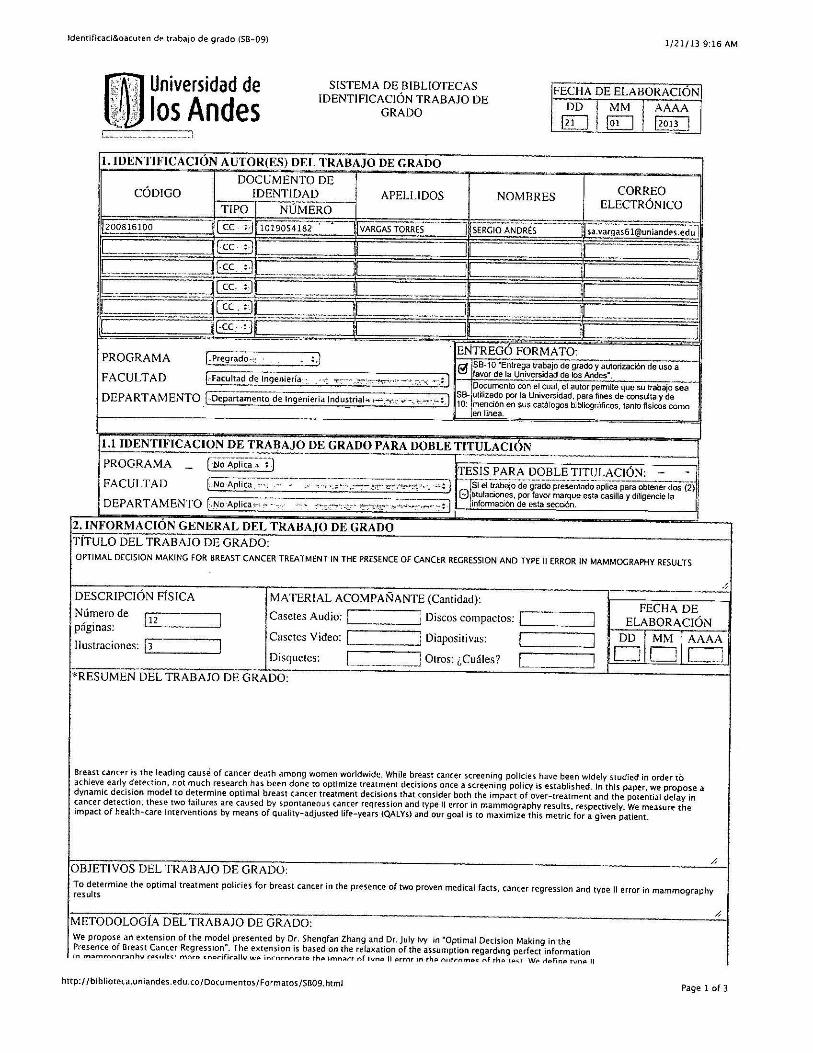
OPTIMAL DECISION MAKING FOR BREAST CANCER TREATMENT IN THE PRESENCEOF CANCER REGRESSION AND TYPE II ERROR IN MAMMOGRAPHY RESULTS

Sergio Andres Vargas Torres

Universidad de los AndesCra 1 A No. 18-10

Bogota D.C., COLOMBIA

Raha Akhavan-Tabatabaei

Universidad de los AndesCra 1 A No. 18-10

Bogota D.C., COLOMBIA

Shengfan Zhang

University of ArkansasFayetteville, AR 72701, USA

ABSTRACT

BREAST cancer is the leading cause of cancer death among women worldwide. While breast cancerscreening policies have been widely studied in order to achieve early detection, not much research

has been done to optimize treatment decisions once a screening policy is established. In this paper, wepropose a dynamic decision model to determine optimal breast cancer treatment decisions that considerboth the impact of over-treatment and the potential delay in cancer detection; these two failures are causedby spontaneous cancer regression and type II error in mammography results, respectively. We measurethe impact of health-care interventions by means of quality-adjusted life-years (QALYs) and our goal is tomaximize this metric for a given patient.

Keywords: Breast cancer, screening policies, treatment decisions, cancer regression, mammography, QALY

1. INTRODUCTION

Breast cancer is often defined as an uncontrolled growth of breast cells caused by a genetic abnormality.In 2011, the American Cancer Society (ACS) estimated more than 450,000 deaths caused by breast cancerand more than 1,000,000 new cases worldwide (Jemal et al. 2011). The same year, according to the ACS,the lifetime risk of developing invasive female breast cancer was about 12%.

Mammography is currently considered to be the most effective technology for population-based breastcancer screening. A mammogram is an x-ray image to examine female breast. The benefits of mammogra-phy include early detection of breast cancer as it can identify problems before any symptoms (e.g. lumps)appear. There have been randomized clinical trials indicating that mammography may reduce breast cancermortality by at least 24% (Kerlikowske et al. 1995, Fracheboud et al. 2006). However, there are two typesof risk that need to be considered when performing mammography. Similar to other binary tests, mammog-raphy has two statistical measures of performance, sensitivity and specificity. Sensitivity is the probabilityof detecting breast cancer when it is truly present while specificity is the probability of correctly identifyinga patient as normal when no cancer exists (Harris et al. 2000). The possible failures generated by specificityand sensitivity have raised the need to take into account this fact when developing optimal mammogra-phy screening policies for various populations (Ayer et al. 2011, Maillart et al. 2008, Michaelson et al. 1999).

Vargas, Akhavan-Tabatabaei, and Zhang

In most screening and treatment decision models, breast cancer is typically modeled as a progressivedisease, under the assumption that cancer does not disappear in the absence of treatment. For example, theMarkov chain model proposed by Chen et al. (1996) is often presented to describe the natural history ofbreast cancer, only allowing an early state of cancer to transition to a more advanced cancer state, or to anabsorbing death state. However, there has been medical evidence suggesting that at an early stage, breastcancer may actually spontaneously regress without treatment (Lewison 1976). While there has been a lotof debate in the medical community regarding cancer regression, there has been limited research about theconsequences of considering this medical fact when determining treatment policies.

Zhang and Simmons (2012b) proposed a finite-horizon Markov decision process (MDP) to establishan optimal treatment policy in the presence of breast cancer regression. Their model assumed perfectinformation in screening results and fixes ACS recommendations reported in (Smith et al. 2009) as thescreening policy upon which treatment decisions are made. The objective of their model is to maximize theQALYs that a patient may lose due to over-treatment. Finally their results showed a significant participationof no-treatment decisions in patients diagnosed with non-invasive breast cancer.

We propose an extension of the model presented by Zhang and Simmons (2012b) that is based onthe relaxation of the assumption regarding perfect information in mammography results; more specificallywe incorporate the impact of type II error in the outcomes of the test. We define type II error as a falsenegative result caused by the sensitivity of mammography and incorporate this failure in our model. Therest of the paper is organized as follows. In §2, we review medical background related to our problem. In§3 we describe the model for optimal treatment policies. In §4 we present our computational experimentsand results. Finally §5 concludes the paper and outlines the future work.

2. MEDICAL BACKGROUND

2.1 Cancer Regression

The literature review on medical exploration of breast cancer spontaneous regression has been summarizedby Zhang and Simmons (2012a). Multiple sources (Osler 1901, Lewison 1976, Larsen and Rose 1999,Burnside et al. 2006) have indicated that although the phenomenon is rare, there is ample evidence toconfirm that spontaneous regression of breast cancer does exist, and thus it should not be ignored. Since thecurrent protocol recommends women to seek treatment after diagnosis, it is difficult to observe the naturalhistory of breast cancer progression and regression. And thus, it is not easy to calculate the probability ofbreast cancer regression directly.

Another important literature to note is the study by Zahl et al. (2008). They compared the number ofinvasive cancers in a six-year period between a control group and a screening group with similar background,and found that the case number in the control group was approximately 22% lower. They concluded thatthe difference was that some screen-detected breast cancer cases may spontaneously regress. In our study,we assume a regression probability of 15% and compare our results with the case where no regression isincorporated.

2.2 Imperfection in mammography results

The success of mammography screening programs depends on accurate examinations and interpretationof results. Mammographic interpretation has two stages, detection and classification. At the detectionstage, a physician examines the x-ray image looking for potential or existing abnormalities in the breasttissue. Once an abnormality is detected, the physician proceeds to classify the finding by means of aninternationally used lexicon designed by the American College of Radiology through the Breast ImagingReporting and Data System (BI-RADS). This human intervention makes mammography results be subject


to possible failure when interpreting mammographic images.

Several studies have shown differences among radiologists when interpreting mammograms (Beamet al. 1996, Karssemeijer et al. 2003, Sickles et al. 2002). Kerlikowske et al. (1998) observed interpretationdifferences among two radiologists with wide experience reading mammograms, finding the overall sensi-tivity ranging from 72.8% to 78.2% in a study that considered 71,713 screening examinations. Elmore andCarney (2002) claim clinically significant variation exists among radiologists interpreting mammograms,they suggested the variation may be attributed to personal, clinical, financial and legal characteristicsof the radiologists, and/or the characteristics of the mammography facility. Beam et al. (2003) tested110 radiologists that interpreted screening mammograms from the same 148 women. They found thatsensitivity in the sample of radiologists ranged from 59% to 100%, and specificity ranged from 35% to98%. In addition, they discussed how lack of skill maintenance or improvement mechanisms may affectthe interpretation of mammographic images.

The duration of observation by a radiologist has been studied and reported as a determinant factor thatincreases sensitivity of mammography results. Nodine et al. (2002) noted that mammographers detected71% of the true lesions within 25 seconds, and trainees detected 46% within 40 seconds. Krupinski (2005)observed that elongated visual dwell times contribute significantly to the detection of subtle findings, andtherefore these mammographic lesions are associated with significantly different visual search parametersthan obvious lesions

3. METHODS

3.1 Model Formulation

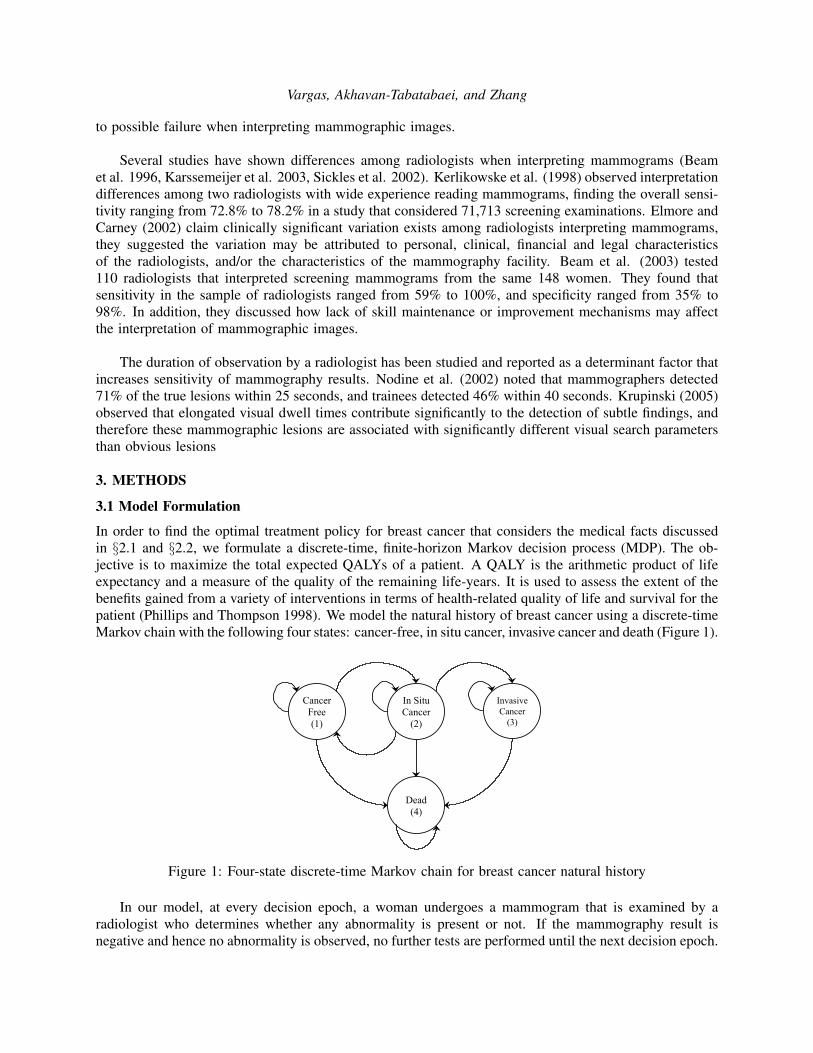
In order to find the optimal treatment policy for breast cancer that considers the medical facts discussedin §2.1 and §2.2, we formulate a discrete-time, finite-horizon Markov decision process (MDP). The ob-jective is to maximize the total expected QALYs of a patient. A QALY is the arithmetic product of lifeexpectancy and a measure of the quality of the remaining life-years. It is used to assess the extent of thebenefits gained from a variety of interventions in terms of health-related quality of life and survival for thepatient (Phillips and Thompson 1998). We model the natural history of breast cancer using a discrete-timeMarkov chain with the following four states: cancer-free, in situ cancer, invasive cancer and death (Figure 1).

Cancer Free (1)

In Situ Cancer

(2)

Invasive Cancer

(3)

Dead (4)

Figure 1: Four-state discrete-time Markov chain for breast cancer natural history

In our model, at every decision epoch, a woman undergoes a mammogram that is examined by aradiologist who determines whether any abnormality is present or not. If the mammography result isnegative and hence no abnormality is observed, no further tests are performed until the next decision epoch.


On the other hand, if the mammography result turns out to be positive, a follow-up biopsy test is performedin order to confirm the existence of cancer. As reported in the literature, breast biopsy sensitivity is veryclose to 100% (Gur et al. 2005), and therefore this test is assumed to be perfect.

We assume that whenever the observed state of a patient is cancer-free, the decision that will be madeis to wait. In addition, if a patient is diagnosed with invasive cancer, the decision maker will alwaysdecide to treat that patient. These assumptions have been studied and established as optimal in medicalguidelines regarding breast cancer treatment (Carlson 2012). However, when the observed state is in situ(non-invasive) cancer, our study does not consider treatment as the only option, whereas the current policiesalways do. Figure 2. presents the decision process our model assumes for breast cancer detection.

Suspicious abnormality? Biopsy

Yes

No

Periodic mammography

Treatment according to pathological

findings

Treat?

No

Yes

Invasive Cancer

In situ Cancer

Figure 2: Decision process for breast cancer early diagnosis and treatment

It is worth mentioning that our model does not include type I error in mammography results (falsepositive results) Therefore, a positive outcome in mammography always implies the patient has eithernon-invasive or invasive cancer since perfect biopsy tests are used to confirm the presence of the disease.On the contrary, type II error is considered and hence a negative result in mammography does not necessarilyimply the patient is healthy. Our MDP components are defined below:

• Set of decision epochs ϒ = 40,41,42, ...,100. According to the ACS recommendation, a womanshould receive annual mammography screening from the age of 40 (Smith et al. 2009). We adoptthis ACS recommendation as the screening policy of our model and define the upper boundary oflife as 100 years in accordance with the maximum life span reported in the United States Life Tablefor 2012 (Arias 2012).

• State space S = 1,2,3,4, where the cancer state of a patient at decision epoch t is definedas st ∈ S ∀ t ∈ ϒ. In particular, 1 represents a cancer-free patient, 2 represents a patient within situ (non-invasive) cancer, 3 represents a patient with invasive cancer and 4 represents a death state.

• Post-diagnosis cancer distribution is denoted by Qt(S) ∀ t ∈ ϒ. We define the post-diagnosis cancerdistribution as a discrete probability distribution over all elements of S once the diagnosis procedureis finished. The element q t

s represents the probability that the state of a patient is s at decisionepoch t after the patient has undergone a mammogram or a mammogram and a biopsy test and


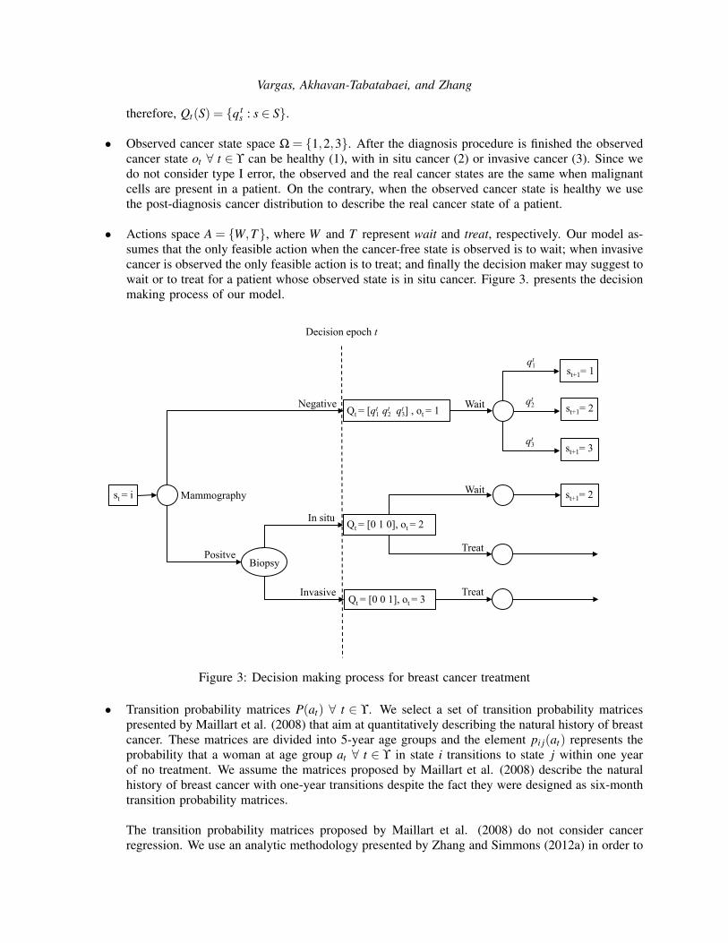
therefore, Qt(S) = q ts : s ∈ S.

• Observed cancer state space Ω = 1,2,3. After the diagnosis procedure is finished the observedcancer state ot ∀ t ∈ ϒ can be healthy (1), with in situ cancer (2) or invasive cancer (3). Since wedo not consider type I error, the observed and the real cancer states are the same when malignantcells are present in a patient. On the contrary, when the observed cancer state is healthy we usethe post-diagnosis cancer distribution to describe the real cancer state of a patient.

• Actions space A = W,T, where W and T represent wait and treat, respectively. Our model as-sumes that the only feasible action when the cancer-free state is observed is to wait; when invasivecancer is observed the only feasible action is to treat; and finally the decision maker may suggest towait or to treat for a patient whose observed state is in situ cancer. Figure 3. presents the decisionmaking process of our model.

Mammography

st = i

Positve

Negative

Biopsy

In situ

Invasive

Qt = [0 1 0], ot = 2

Qt = [0 0 1], ot = 3

Qt = [qt1 qt2 qt3] , ot = 1 st+1= 2

st+1= 2

st+1= 1

st+1= 3

qt1

qt2

qt3

Wait

Wait

Treat

Treat

Decision epoch t

Figure 3: Decision making process for breast cancer treatment

• Transition probability matrices P(at) ∀ t ∈ ϒ. We select a set of transition probability matricespresented by Maillart et al. (2008) that aim at quantitatively describing the natural history of breastcancer. These matrices are divided into 5-year age groups and the element pi j(at) represents theprobability that a woman at age group at ∀ t ∈ ϒ in state i transitions to state j within one yearof no treatment. We assume the matrices proposed by Maillart et al. (2008) describe the naturalhistory of breast cancer with one-year transitions despite the fact they were designed as six-monthtransition probability matrices.

The transition probability matrices proposed by Maillart et al. (2008) do not consider cancerregression. We use an analytic methodology presented by Zhang and Simmons (2012a) in order to


include breast cancer regression. An example of a transition probability matrix from Maillart et al.(2008) is presented below:

P(at)=

p11(at) p12(at) 0 0 p15(at)

0 p22(at) p23(at) 0 p25(at)

0 0 p33(at) p34(at) p35(at)

0 0 0 1 0

0 0 0 0 1

1→ Cancer Free2→ In situ Cancer3→ Invasive Cancer4→ Death by Breast Cancer5→ Death by other reasons

Zhang and Simmons (2012a) proposed the following modification to the original matrix for includingcancer regression.

P?(at)=

p11(at) p12(at) 0 0 p15(at)

p21(at) p∗22(at) p∗

23(at) 0 p25(at)

0 0 p33(at) p34(at) p35(at)

0 0 0 1 0

0 0 0 0 1

p21(at) = u · p22(at)+ v · p23(at)

p∗22(at) = (1−u) · p22(at)

p∗23(at) = (1− v) · p23(at)

0≤ u,v≤ 1

Where u and v are fractions of the self-loop and the progression transition probabilities respectively;these proportions are used to extract information from the existing probabilities and build theregression transition.

• Immediate rewards rt(s,a) ∀ st ∈ S, a ∈ A, t ∈ ϒ, At every decision epoch we measure the impactof treatment in terms of QALYs depending on the age, the cancer state and the action. In thisnotation, rt(s,a) represents the total expected QALYs accumulated at decision epoch t, when thecancer state of a patient is s and action a is taken. We use the estimations done by Stout et al.(2006) regarding QALYs at in situ and invasive cancer states when the decision is wait. Theseestimations were derived from EuroQol EQ-5D quality-of-life utility scores along with a series ofmodifications to estimate the QALYs accrued for a woman with in situ or invasive cancer. The EQ-5D is a standardized measure for general health developed by the EuroQol Group (Brooks et al. 1991).

On the other hand, when the decision is treat, our model uses a life expectancy estimation afterthe necessary treatment is performed. Zhang and Simmons (2012b) proposed a methodology toestimate age-specific 5-year QALYs for breast cancer treatment and calculate the expected totalQALY taking into account different survival probabilities depending on cancer state.

• Discount factor λ , We select a discount factor of 0.97 that has been previously used in dynamicdecisions models regarding medical treatment (Chhatwal et al. 2010).

3.2 Type II error in mammography results

Our model considers type II error of mammography results which means no abnormality may be identifiedon the mammogram image when in fact such an abnormality exists. This type of error generates uncertaintyabout the real cancer state of a patient once the mammography result is negative. We model this uncertainty


by means of a discrete probability distribution that describes the cancer state after diagnosis. As seen inFigure 3. when the diagnosis includes a biopsy intervention the uncertainty disappears thanks to the highaccuracy of this test. However, when a negative result is given and no further tests are performed thereexists a positive probability that a woman has in situ or invasive cancer.

As reported in the literature, mammography sensitivity depends on both the age of the patient and thecancer state (Harris et al. 2000). We define sens t

s as the sensitivity at decision epoch t when the cancerstate of a woman is s. Therefore, Qt(S) is defined in terms of the sensitivity as follows:

Qt(S) =[q t

1 q t2 q t

3

]q t

3 = 1− sens t3

q t2 = 1− sens t

2

q t1 = 1−q t

2 −q t3

The mammography sensitivity function is defined in (Maillart et al. 2008). Here, q t1 is implicitly a theoretical

estimation of mammography specificity but as previously mentioned we do not consider the error causedby this statistical measure of performance. The function Qt(S) will be used in §3.3.

Our model also considers the potential misdiagnosis and consequent delay in cancer detection causedby sensitivity. We propose a series of modifications to the transition probability matrices to consider type IIerror in mammography. These modifications are based on the idea that transitions occur between observedcancer states ot and not between real cancer states st as proposed by (Maillart et al. 2008, Zhang andSimmons 2012a). Below, we present the modified matrix that includes breast cancer regression and typeII error in mammography results.

P ′(at) =

p11(at) p12(at) 0 p14(at)

p′21(at) p′

22(at) p′

23(at) p24(at)

p′31(at) 0 p′

33(at) p34(at)

0 0 0 1

p′21(at) = p21(at)︸︷︷︸

Natural transition

+ p22(at) ·

Type II error︷︸︸︷(1− sens t

2)+p23(at) ·

Type II error︷︸︸︷(1− sens t

3)︸︷︷︸Transitions due to imperfect mammography

p′22(at) = p22(at) · sens t

2


3

p′31(at) = p33(at) · (1− sens t

3)


3


3.3 Optimality equations

We denote by Vt(o) the maximum total expected QALYs the patient can attain when the current observedcancer state is o at decision epoch t. Then,

Vt(o) =

∑u∈S

q tu

(rt(u,W )+λ ∑

s′∈Ω

pus′(at)Vt+1(s′))

ot = 1

max

rt(o,W )+λ ∑s′∈Ω

pos′(at)Vt+1(s′)

rt(o,T )ot = 2

rt(o,T ) ot = 3

In case the observation is cancer-free, we use the post-diagnosis cancer distribution to calculate theimmediate and discounted future QALYs that a patient may obtain. On the other hand, if in situ cancer isobserved, the model will decide either to wait or treat depending on the difference between the immediateplus the discounted future QALYs and the estimation of expected QALYs for the remaining life. Finally,when invasive cancer is observed Vt(o) always equals the estimation of expected QALYs for the remaininglife. The terminal values at year 100 for the decision making process are defined bellow:

V100(o) =

∑u∈S

q100u (r100(u,W )) ot = 1

max

r100(o,W )

r100(o,T )ot = 2

r100(o,T ) ot = 3

4. RESULTS

4.1 Computational Experiments

We solve our MDP model to optimality using the Backward Induction algorithm (Puterman 1994). Table1. presents the optimal treatment policy if a given patient is diagnosed with in situ cancer at a givenage. In Table 1, we present four different scenarios. In the first scenario we evaluate the performanceof our model when none of the considerations discussed in §3 regarding cancer regression and type IIerror in mammography results are taken into account. The second scenario includes the modificationsproposed by Zhang and Simmons (2012b) related to cancer regression but does not consider type II errorin mammography results; in this scenario u and v are assumed 0.1 and 0.5, respectively which results in anaverage regression rate of 15%. The third scenario assesses the optimal treatment policy when type II errorin mammography results is taken into account but cancer regression is not. Finally, the fourth scenariopresents the optimal policy including all considerations discussed in §3; this scenario considers the sameu and v vales as in the second scenario to incorporate cancer regression.

4.2 Discussion

In this section we present results for each scenario presented in §4.1.


Table 1: Optimal treatment policy for in situ breast cancerAge No regression Regression Type II Regression Age No regression Regression Type II Regression

and Type II and Type II40 T T T T 71 W W W W41 T T T T 72 W W W W42 T T T T 73 W W W T43 T T T T 74 W W T T44 T T T T 75 T W T T45 T T T T 76 W W W W46 T T T T 77 W W W W47 T T T T 78 W W W W48 T T T T 79 W W W T49 T T T T 80 T W T T50 T T T T 81 W W W W51 T W T T 82 W W W W52 T W T T 83 W W W W53 T W T T 84 W W W W54 T W T T 85 T W T W55 T T T T 86 W W W W56 T W T T 87 W W W W57 T W T T 88 W W W W58 T W T T 89 W W W W59 T W T T 90 W W W W60 T T T T 91 W W W W61 W W T T 92 W W W W62 W W T T 93 W W W W63 W W T T 94 W W W W64 W W T T 95 W W W W65 T W T T 96 W W W W66 W W W W 97 W W W W67 W W W T 98 W W W W68 W W T T 99 W W W W69 W W T T 100 T T T T70 T W T T

Scenario 1. When cancer regression and type II error in mammography results are ignored, a pa-tient between the ages 40-60 (including 60) who is diagnosed with in situ breast cancer should alwaysbe treated. However, for patients older than 60, the recommendation is to wait until the next screeningperiod except at ages 65, 70, 75, 80, 85 and 100. This trend may be explained by the nature of the dataused to describe the natural history of breast cancer; as discussed in §3.1. Our model uses age-specifictransition probability matrices as input. Therefore, the information that the algorithm uses iteratively isupdated every 5 years and causes this behavior. Note that between ages 85-100 there is only two informationupdates since the matrix that describes the natural history of breast cancer is the same for these last 15 years.

Scenario 2. The optimal policy proposed in this scenario clearly reflects the impact of cancer regressionin treatment decisions. As discussed in §2, if cancer regression is ignored, treatment policies may lead toover-treatment and therefore, a decrease in quality of life. Our model handles this undesirable situationby increasing the waiting decisions along the decision horizon. When cancer regression is considered,our model suggests that treatment is the optimal decision for a patient between ages 40-50 (including 50)who is diagnosed with in situ cancer. On the other hand, patients older than 50 should wait until the nextscreening period except at ages 55 and 60.

Scenario 3. In §3.2 we mentioned a potential delay in cancer detection as a direct consequence ofsensitivity of mammography results. When our model only considers type II error in mammography results,the optimal policy shows how this delay is avoided through an increase in treatment decisions. As shownin Table 1, the optimal decisions include treatment till a later age (65) as compared to 60 in Scenario 1,and 50 in Scenario 2. Here, a patient diagnosed with in situ breast cancer should be treated if the diagnosis


is done between ages 40-70 except at ages 66 and 67. When the age exceeds 70, a patient should waituntil the next screening period unless the age is 74, 75, 80 or 85.

Scenario 4. This scenario considers the impact of both cancer regression and type II error in mammog-raphy results. In Scenario 2 and Scenario 3 we showed how the inclusion of cancer regression and type IIerror in mammography results would lead to an increase in waiting and treatment decisions, respectively.Therefore, a simultaneous inclusion of these aspects proposes a trade-off between unnecessary treatmentand delay in cancer detection. The results show that the optimal treatment policy is slightly closer to thecurrent policy in which treatment is always recommended. However, our model suggests a significantly longage range (between ages 80-100) during which wait is the optimal decision if in situ cancer is diagnosed.

5. CONCLUSIONS AND FUTURE WORK

We formulate an MDP model to determine the optimal treatment policies for breast cancer in the presence oftwo proven medical facts, cancer regression and type II error in mammography results. We solve our modelto optimality and obtain results that give an insight about the complexity of this disease. Our study suggeststhat optimal treatment policies for breast cancer might be different from the common recommendationswhen regression and type II error in mammography results are taken into account. Specifically, we showthat when in situ breast cancer is diagnosed, the quality of life may be negatively affected if treatment isalways recommended. In addition, we find a trade-off between over-treatment and late cancer detectionwhen we analyze different scenarios regarding cancer regression and type II error in mammography results;we consider both factors and our results show that treatment may be optimal only for patients under 80 ifin situ cancer is diagnosed.

The contributions of our work include the handling of uncertainty about the real cancer state of a patientthrough the post-diagnosis cancer state and the modifications proposed to incorporate the observed cancerstate in a simple and intuitive way into a dynamic decision model. Also, to the best of our knowledge,the study proposed by Zhang and Simmons (2012b) is the first to consider no treatment decisions forcancer-diagnosed patients and our study contributes to this work by adding factors that may influencetreatment policies. Finally, our study also contributes to the literature of analytical studies for medicaldecision modeling of breast cancer that considers disease regression.

An important step following to this work is to improve both the transition probability matrices used todescribe the natural history of breast cancer and the estimations regarding quality of life. As discussed in§3, the transition probability matrices required by our approach are difficult to estimate and the informationavailable in the literature lacks a more detailed differentiation regarding age and population dependency.A good contribution would be to estimate the natural history of breast cancer using shorter age rangesand to provide more accurate information regarding sensitivity and specificity depending on the age andcancer state. Likewise, it is important to include type I error in mammography results in order to obtainmore realistic results.

REFERENCES

Arias, E. 2012. “United States life tables, 2008”. National Vital Statistics Reports 61 (3).Ayer, T., O. Alagoz, and N. Stout. 2011. “A POMDP approach to personalize mammography screening

decisions”. Operations Research 60 (5): 1019–1034.Beam, C., E. Conant, and E. Sickles. 2003. “Association of volume and volume-independent factors with

accuracy in screening mammogram interpretation”. Journal of the National Cancer Institute 95 (4):282–290.


Beam, C., D. Sullivan, and P. Layde. 1996. “Effect of human variability on independent double reading inscreening mammography”. Academic radiology 3 (11): 891–897.

Brooks, R., S. Jendteg, B. Lindgren, U. Persson, and S. Bjork. 1991. “EuroQol c©: health-related qualityof life measurement. Results of the Swedish questionnaire exercise”. Health Policy 18 (1): 37–48.

Burnside, E., A. Trentham-Dietz, F. Kelcz, and J. Collins. 2006. “An example of breast cancer regressionon imaging”. Radiology Case Reports 1 (2): 27–37.

Carlson, R.W. 2012, January. “NCCN Clinical Practice Guidelines in Oncology (NCCN Guidelines). BreastCancer”.

Chen, H., S. Duffy, and L. Tabar. 1996. “A Markov chain method to estimate the tumour progression ratefrom preclinical to clinical phase, sensitivity and positive predictive value for mammography in breastcancer screening”. The Statistician 45 (3): 307–317.

Chhatwal, J., O. Alagoz, and E. Burnside. 2010. “Optimal breast biopsy decision-making based on mam-mographic features and demographic factors”. Operations research 58 (6): 1577–1591.

Elmore, J., and P. Carney. 2002. “Does practice make perfect when interpreting mammography?”. Journalof the National Cancer Institute 94 (5): 321–323.

Fracheboud, J., J. Groenewoud, R. Boer, G. Draisma, A. de Bruijn, A. Verbeek, and H. de Koning. 2006.“Seventy-five years is an appropriate upper age limit for population-based mammography screening”.International journal of cancer 118 (8): 2020–2025.

Gur, D., L. Wallace, A. Klym, L. Hardesty, G. Abrams, R. Shah, and J. Sumkin. 2005. “Trends inRecall, Biopsy, and Positive Biopsy Rates for Screening Mammography in an Academic Practice”.Radiology 235 (2): 396–401.

Harris, J., M. Lippman, M. Morrow, C. Osborne, and R. Fund. 2000. Diseases of the Breast. LippincottWilliams & Wilkins Philadelphia, PA.

Jemal, A., F. Bray, M. Center, J. Ferlay, E. Ward, and D. Forman. 2011. “Global cancer statistics”. CA: acancer journal for clinicians 61 (2): 69–90.

Karssemeijer, N., J. Otten, A. Verbeek, J. Groenewoud, H. de Koning, J. Hendriks, and R. Holland.2003. “Computer-aided Detection versus Independent Double Reading of Masses on Mammograms”.Radiology 227 (1): 192–200.

Kerlikowske, K., D. Grady, J. Barclay, V. Ernster, S. Frankel, S. Ominsky, and E. Sickles. 1998. “Variabilityand accuracy in mammographic interpretation using the American College of Radiology Breast ImagingReporting and Data System”. Journal of the National Cancer Institute 90 (23): 1801–1809.

Kerlikowske, K., D. Grady, S. Rubin, C. Sandrock, and V. Ernster. 1995. “Efficacy of screening mammog-raphy”. JAMA: the journal of the American Medical Association 273 (2): 149–154.

Krupinski, E. 2005. “Visual search of mammographic images: Influence of lesion subtlety1”. Academicradiology 12 (8): 965–969.

Larsen, S., and C. Rose. 1999. “Spontaneous remission of breast cancer. A literature review”. Ugeskriftfor laeger 161 (26): 4001.

Lewison, E. 1976. “Spontaneous regression of breast cancer”. National Cancer Institute Monograph 44:23.Maillart, L., J. Ivy, S. Ransom, and K. Diehl. 2008. “Assessing dynamic breast cancer screening policies”.

Operations Research 56 (6): 1411–1427.Michaelson, J., E. Halpern, and D. Kopans. 1999. “Breast Cancer: Computer Simulation Method for

Estimating Optimal Intervals for Screening”. Radiology 212 (2): 551–560.Nodine, C., C. Mello-Thoms, H. Kundel, and S. Weinstein. 2002. “Time course of perception and decision

making during mammographic interpretation”. American Journal of Roentgenology 179 (4): 917–923.Osler, W. 1901. The medical aspects of carcinoma of the breast, with a note on the spontaneous disappearance

of secondary growths. Philadelphia: sn.Phillips, C., and G. Thompson. 1998. What is a QALY?, Volume 1. Hayward Medical Communications.Puterman, M. 1994. Markov decision processes: Discrete stochastic dynamic programming. John Wiley &

Sons, Inc.


Sickles, E., D. Wolverton, and K. Dee. 2002. “Performance Parameters for Screening and DiagnosticMammography: Specialist and General Radiologists”. Radiology 224 (3): 861–869.

Smith, R., V. Cokkinides, A. von Eschenbach, B. Levin, C. Cohen, C. Runowicz, S. Sener, D. Saslow, andH. Eyre. 2009. “American Cancer Society guidelines for the early detection of cancer”. CA: a cancerjournal for clinicians 52 (1): 8–22.

Stout, N., M. Rosenberg, A. Trentham-Dietz, M. Smith, S. Robinson, and D. Fryback. 2006. “Retrospectivecost-effectiveness analysis of screening mammography”. Journal of the National Cancer Institute 98(11): 774–782.

Zahl, P., J. Mæhlen, and H. Welch. 2008. “The natural history of invasive breast cancers detected byscreening mammography”. Archives of Internal Medicine 168 (21): 2311.

Zhang, S., and J. Simmons. 2012a. “Analytic Modeling of Breast Cancer Spontaneous Regression”. InProceedings of Industrial and Systems Engineering Research Conference.

Zhang, S., and J. Simmons. 2012b. “Optimal Decision Making in the Presence of Breast Cancer Regression”.In Proceedings of Industrial and Systems Engineering Research Conference.

Documents

OPTIMAL DECISION MAKING FOR BREAST CANCER TREATMENT …