저 시-비 리- 경 지 2.0 한민

는 아래 조건 르는 경 에 한하여 게

l 저 물 복제, 포, 전송, 전시, 공연 송할 수 습니다.

다 과 같 조건 라야 합니다:

l 하는, 저 물 나 포 경 , 저 물에 적 된 허락조건 명확하게 나타내어야 합니다.

l 저 터 허가를 면 러한 조건들 적 되지 않습니다.

저 에 른 리는 내 에 하여 향 지 않습니다.

것 허락규약(Legal Code) 해하 쉽게 약한 것 니다.

Disclaimer

저 시. 하는 원저 를 시하여야 합니다.

비 리. 하는 저 물 리 목적 할 수 없습니다.

경 지. 하는 저 물 개 , 형 또는 가공할 수 없습니다.

공학박사학위논문

Optimal control strategies for gas cooling

systems using geometric design and model

predictive control

구조설계와모델예측제어를사용하는

기체냉각시스템의최적운전전략수립

2016년 6월

서울대학교대학원

화학생물공학부

임유경

Optimal control strategies for gas cooling

systems using geometric design and model

predictive control

지도교수이종민

이논문을공학박사학위논문으로제출함

2016년 12월

서울대학교대학원

화학생물공학부

임유경

임유경의박사학위논문을인준함

2016년 6월

위 원 장 이종협 (인)

부위원장 이종민 (인)

위 원 윤인섭 (인)

위 원 이원보 (인)

위 원 남재욱 (인)

Abstract

Optimal control strategies for gas coolingsystems using geometric design and model

predictive control

Yu Kyung Lim

School of Chemical and Biological Engineering

The Graduate School

Seoul National University

This thesis presents a theoretical approach on designing the geometry of

a gas cooling system unit and its application with the multivariable opti-

mal control technique based on the dynamic mathematical models with

a motivation to enhance the cooling efficiency. The gas cooling system

can be defined as a process that cools down the exterior heat or solid

microparticles introduced to a confined volume space by injecting inert

cooling gas stream that absorbs the released heat. Two example cooling

processes that are discussed in this study and come under this defini-

tion are the CO2 storage tank pre-cooling process and the microparticle

cooling process. Although both processes are included in a same pro-

cess category, the individual process characteristics and their ultimate

goals which need to be achieved are significantly different. Hence, such

factors requiring the main consideration are discussed for the design of

i

the cooling process units. These apply also on developing the optimal

controller scheme for the gas cooling systems. Rigorous dynamic mod-

elings are derived for each process based on the first principles which

are further used in the development of appropriate model predictive con-

trol (MPC) schemes. The result produced by these optimal controllers

are later compared with base cases using the proportional-integral (PI)

controllers, which illustrate that the multivariable optimal control is able

to enhance the stability and the efficiency of both processes.

First example is the pre-cooling process of CO2 storage tanks. The

design of CO2 storage tanks are determined in advance considering the

maximization of the available loading amount. The tank system must

be cooled before loading cryogenic liquid CO2 to prevent physical and

thermal damage to the tank wall. The pre-cooling process gasifies a frac-

tion of the liquid CO2 cargo and injects the resulting gas into the storage

tank until the tank reaches the target temperature and pressure. Thus an

MPC approach for optimizing the injection flowrate of CO2 gas to re-

duce the loss of liquid CO2 cargo and CO2 capturing and compression

cost is proposed. The process is mathematically formulated into a non-

linear multi-input-multi-output (MIMO) gas-phase system in which the

injection mass flowrate and the outlet purging mass flowrate of CO2 gas

act as control inputs. Then, a finite-horizon linearized model predictive

control (MPC) scheme is designed to make the tank system reach the

target state within a designated operation time limit. A terminal penalty

is suboptimally approximated by solving a modified discrete Lyapunov

stability condition and added to the control objective function in order

ii

to provide a theoretical finite-horizon stability and enhance the process

termination.

For the microparticle cooling process which is the second example,

a systematical procedure for selecting a favorite design of a cylinder-

on-cone cooling chamber that provides sufficient cooling residence time

for spherical polymer particles produced by a prototype polymer melt-

spray nozzle is suggested. First, calculations on the particle residence

time required for cooling is carried out using a lumped particle model

to determine the chamber height. Second, dynamic responses with a step

input of the hot air injection rate and the overall air flow streamlines

inside the case examples with different chamber structures are obtained

with computational fluid dynamics (CFD) simulations. The simulation

results suggest that the cone height and the diameters of the cylinder

and the outlet interact each other, influencing the mixing and the heat

transfer of the gas phase inside the cooling chamber. A chamber design

with less instability and good mixing in the air flow is selected among

the case designs. CFD simulation results show that polymer droplets are

sufficiently cooled in the selected chamber geometry.

Lastly, an adaptive MPC structure controlling the air temperature

inside the spray cooling chamber and the flowrate of the purging air out

from the chamber outlet simultaneously by manipulating the injection

flowrates of cold air and normal air streams is devised. The idea is based

on the fact that significant portion of microparticle products depend their

moving trajectories on the gravity and the flowrate of the surrounding air

stream, which make these two variables the main operation parameters

iii

influencing the efficiencies of the follow-up units which collect the mi-

croparticles according to their sizes. We demonstrate that both control

variables are well-managed near given setpoints through the MPC appli-

cation, rejecting three possible scenarios of step disturbances added on

the process parameters including the setpoint of the air temperature in-

side the spray cooling chamber, the surrounding air temperature and the

injection mass flowrate of the melt feed stream.

Keywords: Pre-cooling process, Microparticle cooling process, Model

predictive control, Computational fluid dynamics

Student Number: 2010-21010

iv

Contents

Abstract . . . . . . . . . . . . . . . . . . . . . . . . . . . . . . . i

1. Introduction . . . . . . . . . . . . . . . . . . . . . . . . . 1

2. Pre-cooling process of CO2 storage tank in CCS ship trans-

portation . . . . . . . . . . . . . . . . . . . . . . . . . . . 3

2.1 Introduction . . . . . . . . . . . . . . . . . . . . . . . . 3

2.2 Process description . . . . . . . . . . . . . . . . . . . . . 7

2.3 Process dynamic model . . . . . . . . . . . . . . . . . . 10

2.3.1 Mathematical model . . . . . . . . . . . . . . . . 10

2.3.2 Dynamic model verification . . . . . . . . . . . . 18

2.4 Control problem formulation . . . . . . . . . . . . . . . 20

2.4.1 Discrete MPC . . . . . . . . . . . . . . . . . . . 21

2.4.2 Modified Lyapunov stability condition . . . . . . 22

2.4.3 PI control . . . . . . . . . . . . . . . . . . . . . . 25

2.5 Dynamic simulation results . . . . . . . . . . . . . . . . 30

2.5.1 Effect of the weighting matrix Qt on the Lyapunov

stability around the target state xt . . . . . . . . . 30

2.5.2 Effect of Qt on control input and state variable tra-

jectories . . . . . . . . . . . . . . . . . . . . . . 33

2.5.3 Discussion . . . . . . . . . . . . . . . . . . . . . 37

3. Concluding remarks . . . . . . . . . . . . . . . . . . . . . 39

v

3.1 Summary and contributions . . . . . . . . . . . . . . . . 39

3.2 Suggested future works . . . . . . . . . . . . . . . . . . 40

Bibliography . . . . . . . . . . . . . . . . . . . . . . . . . . . . 41

vi

List of Figures

Figure 1. In-door pilot experiment of CO2 storage tank opera-

tion measuring BOG generation [1] . . . . . . . . . 8

Figure 2. Schematic diagram of the CO2 storage tank and the

pre-cooling process . . . . . . . . . . . . . . . . . . 9

Figure 3. Surface fitting of the heat capacity of CO2 as a func-

tion of temperature and pressure depicted with the

CO2 P -T phase diagram . . . . . . . . . . . . . . . 13

Figure 4. PFD of the pre-cooling process on Aspen HYSYS 7.3 19

Figure 5. Open-loop step response test with the proposed model

and Aspen HYSYS 7.3 (min = 12 ton/h, mout =

10 ton/h); (a) tank pressure in Case 1; (b) tank tem-

perature in Case 1; (c) tank pressure in Case 2; (d)

tank temperature in Case 2 . . . . . . . . . . . . . . 20

Figure 6. Step responses and dynamic RGA results of the pre-

cooling process; top left: step input trajectories of

min and mout, top right: step response trajectory of

P ; bottom left: step response trajectory of T ; bottom

right: dynamic RGA based on Eq. (2.25) . . . . . . 29

Figure 7. The gradient plot around the target state P = 500 kPa,

T = 243.15K . . . . . . . . . . . . . . . . . . . . . 32

vii

Figure 8. Change of Ω along the magnitude of Qt; (a) Case 1;

(b) Case 2; (c) Case 3; (d) Case 4 (yellow zone: area

where Eq. (2.20) is feasible when Qt = Qt; purple

zone: area where Eq. (2.20) is infeasible when Qt =

Qt) . . . . . . . . . . . . . . . . . . . . . . . . . . 33

Figure 9. Dynamic sequences of outputs and control inputs;

column 1: control inputs min and mout; column 2:

trajectory of P ; column 3: trajectory of T ; row 1:

MPC-case 1; row 2: MPC-case 2; row 3: MPC-case

3; row 4: MPC-case 4; row 5: base case-PI control . 35

viii

List of Tables

Table 1. The polynomial fitting coefficients for Cp in Eq. (2.3) . 13

Table 2. Operating parameters of the open-loop step response test 19

Table 3. Control parameters based on [2, 3] . . . . . . . . . . . 29

Table 4. Change in λ(Qt

)with respect to the change of κ . . . 32

ix

Chapter 1

Introduction

A gas cooling system is a cooling process that is generally oper-

ated inside a confined space volume where heat sources carried by outer

materials or exterior energy penetrating through the unit wall are trans-

ferred to the surrounding cooling gas stream, which is well-mixed with

the heat sources within the cooling unit. Unlike cooling agents such as

water or steam, volatile substances including ethanol and fluorine chem-

icals, the cooling materials used in a gas cooling system regarding this

study include nitrogen (N2), carbon dioxide (CO2) and air, all of them

being chemically inert [4]. Such gases do less damage on properties and

shapes of products and reduce the possibility of operation hazards such

as fire and explosions, the latter being strictly managed especially in the

microparticle producing industries [5]. Despite these advantages, they

generally have heat capacities same or lower than the normal air, which

can cause following problems at the actual operation and process design

stages of gas cooling systems using inert gases. First, cooling efficiency

is poor compared to other types of coolants. As an example in a process

that cools miscellaneous particles, the size of the process system may

1

become considerably large in order to provide sufficient length of par-

ticle residence time (PRT) inside the cooling unit. Second, the volume

of the cooling gas used in process can rise to an extensive amount due

to low density, making it difficult to cope with the rising pressure inside

process units and increasing the operation cost having to spend more

on the cooling power supply. To tackle these problems concerning gas

cooling systems, a systematic approach with a theoretical background on

designing the geometry of a given gas cooling process unit and applica-

tion of the optimal control technology which can successfully manipulate

multivariable interactions among the process variables are discussed. In

this thesis, two process examples including the pre-cooling process of

the CO2 storage tank unit and the microparticle cooling process produc-

ing polymer particle products using a melt-spray system are studied fol-

lowing the research topics explained above. Although these processes

are loosely connected with each other in the sense that they use similar

means of cooling, their ultimate goals are different which require sepa-

rate point of view in conducting the research. More detailed descriptions

and definition of the study objectives are provided in later sections.

2

Chapter 2

Pre-cooling process of CO2 storage tank in CCS

ship transportation

2.1 Introduction

A CO2 carrier is a means for transporting liquid CO2 via ship, which

is part of the carbon capture and storage (CCS) chain. Its role is to ship

liquid CO2 waste produced from the onshore CO2 capture and liquefac-

tion process, transport it to an offshore storage site and support the injec-

tion process into suboceanic strata [6]. Although CO2 carriers are more

economical than CO2 pipelines when the amount of the cargo is small

and the shipping distance is greater than approximately 1000 km [7, 8], a

case study has shown that the CO2 transportation cost of CO2 pipelines is

lower than that of CO2 carriers when the transportation process is limited

to the case of South Korea [9]. Therefore, detailed studies on the entire

loading/unloading and shipping process operations of CO2 carriers are

necessary to determine their optimal operating conditions and to ensure

a competitive edge over the pipeline networks. The pre-cooling process

is operated prior to the actual shipping, and this process pushes the tank

3

pressure and temperature closer to those of liquefied CO2 cargo with va-

porized CO2, starting from an initial condition of (300 kPa, 293.15K)

and shifting towards (500 kPa, 243.15K). The purpose of this process is

to protect the stability of the wall material from thermal deformation and

to reduce the generation of boil-off gas (BOG) during onloading [10]. In

this study, an optimal control problem of the pre-cooling process is for-

mulated to enhance the process efficiency and to reduce the amount of

cooling gas injection, since excessive use of cooling gas would lead to

the loss of capturing and liquefying cost of CO2.

In order to find the efficient operation of this process, several im-

portant considerations should be taken into account: first, the pressure of

the CO2 storage tank should be controlled in addition to the tank tem-

perature; overpressure of the tank might cause backflow while the liquid

CO2 of a cargo flows into the tank. In contrast, a low tank pressure might

result in the excessive generation of boil-off gas during the loading pro-

cess. Second, the pre-cooling process needs to be completed within a

predetermined time because it is advantageous to keep the time spent on

waste material transport as short as possible. At the same time, the rec-

ommended maximum cooling rate of the storage tank should be kept at

approximately −10K/h to prevent any damage from thermal brittling. Fi-

nally, it is necessary to develop a dynamic model of the pre-cooling pro-

cess and provide an optimal input sequence that controls the tank pres-

sure and temperature while minimizing the injection and outlet purging

mass flowrates of the cooling gas.

Previous studies on gas storage tank control systems generally fo-

4

cus on tank pressure controllers because they are sufficient for regulating

the tank temperature due to a self-pressurization effect without requiring

additional temperature controllers [11, 12]. For example, BOG regula-

tion for cryogenic liquefied natural gas (LNG) storage tanks has been

achieved using single-input-single-output (SISO) proportional-integral-

derivative (PID) controllers, which manipulate the outlet purging gas

flowrate to maintain the tank pressure, and there has been no need to

minimize the outlet purging flowrate because boil-off LNG could be uti-

lized as fuel [13]. From the industrial point of view, the pre-cooling pro-

cess has been an essential step in the start-up process of on-shore LNG

tanks and facilities which comes before the un-loading of the LNG cargo

[14, 15]. In a case of the Pyeontaek LNG terminal in South Korea man-

aged by the Korea Gas Corporation (KOGAS), a continuous circulation

of low-pressure LNG gas lowers the temperature of the unloading fa-

cilities. Since the terminal lines are directly connected to nearby power

plants and automobile manufacturing factories, some of the LNG gas

used in pre-cooling are utilized as an energy source [16]. By contrast,

CO2 BOG is inherently a waste material, and therefore its outlet purging

mass flowrate requires minimization as the CO2 BOG generation should

lower the economic efficiency of the CCS process.

Considering the above, this part of research develops a nonlinear

mathematical model of the pre-cooling process of CO2 storage tanks

and calculate an optimal control input sequence using the MPC algo-

rithm to compensate linearization error and handle input constraints. The

MPC algorithm has been applied on various industries including Shell

5

Oil starting from 1970s [17]. Compared to a simple feedback based con-

trol, it provides significant improvements in multivariable processes in-

cluding an LNG plant such as reducing the process output instabilities

and increasing profit by pushing the operation condition closer to opti-

mal limit [18]. A terminal penalty must be added to the control objective

to form a finite-horizon MPC as well as to complete the process within

the time limit. This terminal penalty is obtained by solving a Lyapunov

stability condition in the case of a linear state space problem, but this is

not possible with a nonlinear problem unless an iterative calculation is

adopted [19, 20]. In this study the process system is linearized at the tar-

get state for the formation of a linear MPC scheme. However, the system

is an integrating process with the target state being a critical equilibrium.

Since the terminal penalty is difficult to obtain through the Lyapunov

stability condition in such a case, this study uses a suboptimal method

to approximate the weighting matrix of a quadratic terminal penalty.

Several candidates of the weighting matrix of the terminal penalty are

obtained by solving a modified linear Lyapunov stability condition in

which a slack variable is added. We select four of these candidates that

satisfies the original nonlinear Lyapunov stability condition. Some re-

sults from this suboptimal selection occasionally destabilize the MPC

because the resulting terminal penalty terms are large compared to other

terms in the control objective; hence, the effects of the value of the termi-

nal penalty on the resulting optimal input and output sequences are also

considered. Finally the MPC results are compared with a base case of the

proportional-integral (PI) control application in order to demonstrate that

6

the MPC is more advantageous in securing the process stability than the

PI controller.

2.2 Process description

Design of the storage tank geometry must consider the fact that the

tank system shall eventually be installed on board. Therefore its blueprints

confirmed by the contractors in advance focus mainly on maximizing the

loading amount of liquid CO2 cargo within a confined space volume,

rather than considering the pre-cooling process which is one of the in-

termediary step during the tank pretreating procedure. Taking such fac-

tors into account, the tank is designed in a bi-lobe shape with maximum

capacity of 13 000m3. A pilot experiment including two down-scaled bi-

lobe tanks with a capacity of 40m3 each depicted in Fig. 1 was con-

ducted in 2013 in order to analyze the BOG generation when the tanks

operate in a cryogenic condition while the exterior surrounding had room

temperature [1].

A desirable operating scenario regarding the pre-cooling process is

to inject CO2 cooling gas at 225.15K into a tank initially filled with CO2

to increase the tank pressure from 300 kPa to 500 kPa and to cool the

storage tank temperature from 293.15K to 243.15K, where the main op-

erating unit in the pre-cooling process is the CO2 storage tank with an

ellipsoidal shape in the horizontal direction. Fig. 2 shows a simplified

process flow diagram that includes the storage tank and the peripheral

units. The tank wall is composed of carbon steel, and its outer surface is

7

Figure 1: In-door pilot experiment of CO2 storage tank operation measuringBOG generation [1]

covered with polyurethane spray foam, which acts as the insulation layer

of the cryogenic tank.

PT TT

CO2 storage tank

MPC

Cooling CO2 gas

Vent Outflow

Figure 2: Schematic diagram of the CO2 storage tank and the pre-cooling pro-cess

The actual pre-cooling process involves a tank system in which the

tank pressure and temperature are defined non-ideally. An analysis of the

8

system with a high accuracy could be provided by a commercial pro-

cess simulator by iteratively solving a cubic equation of state such as

the Peng-Robinson equation. However, an equally important objective of

this study besides the accuracy is to provide a clear analysis on how the

state variables interact thermodynamically with the heat sources added

to the system. Since such information is difficult to obtain from simu-

lator models, a mathematical model comprised of ordinary differential

equations (ODEs) describing the dynamics of the state variables is newly

developed based on the mass and energy balances. As our method of de-

veloping the mathematical model involves a step that differentiates the

equation of state, the ideal gas law is employed in order to simplify the

differentiation step and the resulting ODEs. The usage of the ideal gas

law is verified by comparing the value of the compressibility factors Z of

both the Peng-Robinson equation and the ideal gas law and using a sim-

ulation result from a process simulator environment in the later sections.

An additional consideration is given to the specific heat capacity of

CO2. The functional relationship between the specific heat, the temper-

ature and the pressure is identified based on a published experimental

data. Other minor assumptions are given at the end of this section.

2.3 Process dynamic model

A mathematical model of the pre-cooling process is required in order

to develop an optimal control scheme. The first part of this section shows

the steps for developing nonlinear differential equations that describe the

9

system dynamics based on the mass and energy balances and the ideal gas

law. The reliability of this mathematical model is tested in the second part

by comparing the open-loop step responses with those of a commercial

process simulator.

2.3.1 Mathematical model

The Peng-Robinson equation of state is common choice for the ther-

modynamic modeling of cryogenic liquid-gas systems, such as LNG stor-

age tanks [21, 22]. This equation of state produces more accurate ther-

modynamic values for this particular circumstance than the ideal gas law.

The Peng-Robinson equation of state and the ideal gas law are stated in

Eqs. (2.1a-2.1b), respectively, where P is the pressure, T is the temper-

ature, R is the ideal gas constant, and Vm is the molar volume. Detailed

descriptions of other accompanying parameters in Eq. (2.1a) are provided

in [23].

P =RT

Vm − b− a (T )

Vm (Vm + b) + b (Vm − b)(2.1a)

P =RT

Vm

(2.1b)

When the condition of a CO2 storage tank changes from the initial state

(300 kPa, 293.15K) to the target state (500 kPa, 243.15K), the compress-

ibility factor Z = PVm

RTcalculated using the Peng-Robinson equation of

state changes from 0.9826 to 0.9487. These values are close to one and

therefore employing Eq. (2.1b) for the thermodynamic modeling is re-

10

garded as valid. Justification of the use of the ideal gas law in a cryo-

genic gas system by calculating the value of Z is also stated in [24]. We

compromise the model accuracy and consider that the ideal gas law is

sufficient for describing the general tendency of the change in the tank

dynamics.

As for the specific heat capacity inside a system with a constant vol-

ume, it is originally derived from the specific internal energy that is ex-

pressed as a function of temperature and volume [25]. The differentiated

specific internal energy is shown in Eq. (2.2),

dU =

(∂U

∂T

)V

dT +

(∂U

∂V

)T

dV (2.2)

where Cv =(∂U∂T

)V

is the specific heat capacity at a constant V .

The value of Cv should theoretically depend only on T when the gas is

supposed to be ideal. However this is not directly usable in our case with

a non-ideal cooling gas. Hence the specific heat capacity inside the tank

system is defined as a function of T and P . For this study, experimental

measurements of Cp of CO2 within the range between 0.5 bar - 20 bar and

200K - 700K from [26] are used to fit a 5th-order polynomial function

of T and P , as shown in Eq. (2.3). Later the values of Cp are multi-

plied by a constant value to result in the corresponding values of Cv. The

coefficients calculated by least squares are shown in Table 1. The sum

of squared errors (SSE) and R-squared values of Eq. (2.3) are 0.1138

and 0.9708, respectively, whereas a higher-order fitting with either P or

T does not lead to a meaningful improvement. The resulting function

11

shown in Fig. 3 indicates that Eq. (2.3) shows an acceptable agreement

with the literature data.

200300

400500

600700 0

1000

2000

0.8

1

1.2

1.4

P [kPa]

T [K]

Cp

[kJ/t

on

K]

Surface fitting

Lite ra ture da ta

Gas

Liquid

Solid

Triple point at

(216.55K, 518kPa)

Figure 3: Surface fitting of the heat capacity of CO2 as a function of temperatureand pressure depicted with the CO2 P -T phase diagram

Cp =g (T, P )

=a0,0 + a0,1T + a0,2T2 + a0,3T

3 + a0,4T4 + a0,5T

5

+a1,0P + a1,1PT + a1,2PT 2 + a1,3PT 3 + a1,4PT 4

(2.3)

Further assumptions used for modeling are as follows:

12

Table 1: The polynomial fitting coefficients for Cp in Eq. (2.3)

Coefficient Value Coefficient Valuea0,0 1.968× 103 a1,0 3.129a0,1 −18.14 a1,1 −2.303× 10−2

a0,2 9.282× 10−2 a1,2 6.255× 10−5

a0,3 −2.078× 10−4 a1,3 −7.388× 10−8

a0,4 2.175× 10−7 a1,4 3.197× 10−11

a0,5 −8.665× 10−11

• The amount of cooling gas condensed to liquid is negligible. In

addition the tank system is initially in a single-element (CO2) gas

phase because it is assumed that the tank undergoes a moisture dry-

ing process by injecting the CO2 gas to replace the air with mois-

ture.

• The storage tank does not make direct contact with cradle supports.

Therefore, the heat flowrate into the tank through the walls is as-

sumed to be equal at every location of the tank walls.

• The difference between the temperature of the inner and outer sides

of the steel layer of the tank wall is negligible because the heat

transfer resistance of the steel layer is significantly less than that of

the insulation layer.

The mathematical model includes ODEs of the tank pressure P and

temperature T , which are derived from the mass and energy balances of

the tank system shown in Eqs. (2.4a-2.4d), where M and E are the total

amount of mass and energy inside the tank, respectively; q is the exter-

nal heat source term; min is the rate of the injection mass flowrate; mout

is the rate of outlet purging mass flowrate; ein and eout are the specific

13

enthalpies of injection and outlet purging streams of the storage tank,

respectively; Cp,in and Tin are the specific heat capacity and the temper-

ature of the injection stream, respectively; Cp and T are the specific heat

capacity and the temperature of the tank inside and the outlet purging

stream, respectively; Pref is the reference pressure and Tref is the refer-

ence temperature.

dM

dt= min −mout (2.4a)

dE

dt= ein − eout + q (2.4b)

ein − eout = (2.4c)

min

∫ Pin

Pref

∫ Tin

Tref

CpdTdP −mout

∫ P

Pref

∫ T

Tref

CpdTdP

Equations for q are shown in Eqs. (2.5a-2.5b). u is the overall heat trans-

fer coefficient, which is a function of Tex, the temperature of the external

environment; hex is the external heat convection coefficient; Lins is the

thickness of the insulation layer of the tank wall; kins is the heat conduc-

tivity of the insulation layer; htank is the convective heat transfer coeffi-

cient inside the tank; Lstl is the thickness of the steel layer of the tank

wall; and kstl is the heat conductivity of the steel layer. Tw1 in Eq. (2.5c)

is the temperature of the steel layer. It is derived by rearranging Eq. (2.5a)

and can be separately calculated after the value of T is obtained at each

14

time step.

q

A= u (Tex − T ) = htank (Tw1 − T ) (2.5a)

u =1

1/hex + Lins/kins + Lstl/kstl + 1/htank

(2.5b)

Tw1 = T +u

htank

(Tex − T ) (2.5c)

Above definitions of mass and energy balances can be related to the

ODEs of P and T by converting the ideal gas law in Eq. (2.6) as functions

of M and T , where Mg is the molar mass and V is the tank volume.

PV =M

Mg

RT (2.6)

Eq. (2.6) is modified and differentiated in time considering V being con-

stant, resulting Eq. (2.7a) and Eq. (2.7b).

dM

dt=

VMg

R

d

dt

(P

T

)(2.7a)

d (MT )

dt=

VMg

R

dP

dt(2.7b)

The mass balance in Eq. (2.4a) is then combined with Eq. (2.7a) to pro-

duce the dynamic model equation of T in Eq. (2.8).

dT

dt=

T

P

dP

dt− R

VMg

T 2

P(min −mout) (2.8)

Eq. (2.9) is the first step for deriving dPdt

. It shows that dEdt

in Eq. (2.4b) is

15

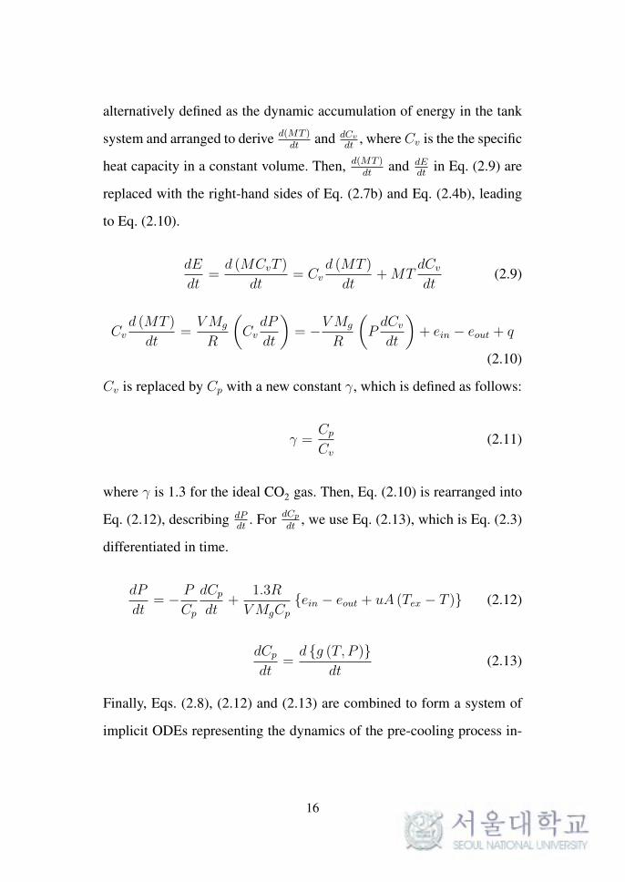
alternatively defined as the dynamic accumulation of energy in the tank

system and arranged to derive d(MT )dt

and dCv

dt, where Cv is the the specific

heat capacity in a constant volume. Then, d(MT )dt

and dEdt

in Eq. (2.9) are

replaced with the right-hand sides of Eq. (2.7b) and Eq. (2.4b), leading

to Eq. (2.10).

dE

dt=

d (MCvT )

dt= Cv

d (MT )

dt+MT

dCv

dt(2.9)

Cvd (MT )

dt=

VMg

R

(Cv

dP

dt

)= −VMg

R

(PdCv

dt

)+ ein − eout + q

(2.10)

Cv is replaced by Cp with a new constant γ, which is defined as follows:

γ =Cp

Cv

(2.11)

where γ is 1.3 for the ideal CO2 gas. Then, Eq. (2.10) is rearranged into

Eq. (2.12), describing dPdt

. For dCp

dt, we use Eq. (2.13), which is Eq. (2.3)

differentiated in time.

dP

dt= − P

Cp

dCp

dt+

1.3R

VMgCp

ein − eout + uA (Tex − T ) (2.12)

dCp

dt=

d g (T, P )dt

(2.13)

Finally, Eqs. (2.8), (2.12) and (2.13) are combined to form a system of

implicit ODEs representing the dynamics of the pre-cooling process in-

16

side a tank with a constant volume.

d

dt

PT

=

− PCp

dCp

dt+ 1.3R

VMgCpein − eout + uA (Tex − T )

TP

dPdt

− RVMg

T 2

P(min −mout)

(2.14)

If the tank system is well insulated, the main driving forces that change

P and T are the enthalpy values relevant to min and mout. The right-hand

side of dPdt

shows that P rises when T is lowered as the result of increas-

ing min. However, the negative second term on the right-hand side of dTdt

shows that its absolute value is reduced by increasing P in the denomina-

tor. Injecting cooling gas excessively and increasing P have advantages

since they prevent BOG formation during the actual loading afterwards.

However the mathematical model indicates that letting P to be increased

indefinitely does not have a positive effect on the efficiency of the pre-

cooling process, rather wasting the cooling gas. As a result the model

shows the interaction between P and T of the storage tank and describes

how these variables may be controlled by the potential manipulated in-

puts min and mout, whereas such an explanation of the process is difficult

to obtain with black box models in commercial process simulators.

2.3.2 Dynamic model verification

The reliability of the model should be verified with experimental

data. However because thermodynamic experimental data of the CO2

storage tank during the pre-cooling process is not available, the accuracy

of the mathematical model is validated by comparing two example cases

17

of the open-loop simulation results from Eq. (2.14) and the process flow

diagram (PFD) in Aspen HYSYS 7.3 environment in Fig. 4. The main

purpose of the test is to verify whether it is acceptable to use the assump-

tion of the ideal gas law in developing Eq. (2.14). For the Aspen HYSYS

7.3 simulations, the Peng-Robinson equation of state is employed. The

valve opening of V2 in Fig. 4 is set to zero since the condensed liquid

CO2 is not released from the storage tank in a real pre-cooling process.

Figure 4: PFD of the pre-cooling process on Aspen HYSYS 7.3

The initial condition of Case 1 is 101.3 kPa, 293.15K, and the initial

condition of Case 2 is 300.0 kPa, 278.15K. min and mout in both cases

are initially zero, which are changed to 12 ton/h and 10 ton/h respectively

when the dynamic simulation starts. The other operating parameters are

specified in Table 2. Fig. 5 presents the result of open-loop step response.

We conclude that the mathematical model exhibits an acceptable agree-

ment with the results of Aspen HYSYS 7.3 and a satisfactory description

of the process dynamics despite using the ideal gas law.

18

Table 2: Operating parameters of the open-loop step response test

Parameter Description ValueA Outer surface area of tank [m2] 2.026× 103

Cp,in Specific heat capacity of CO2 [kJ/ton/K] 824.61L Thickness of tank wall insulation layer (polyurethane) [m] 0.30Mg Molar weight of CO2 [ton/kmole] 44.01× 10−3

R Ideal gas constant [kJ/kmole/K] 8.3145Tex External environment temperature [K] 293.15Tin Mass inflow temperature [K] 225.15V Tank volume [m3] 1.30× 104

hex External heat convection coefficient [kJ/m2/h/K] 10.44htank Internal heat convection coefficient [kJ/m2/h/K] 15.00k Heat conductivity of tank wall insulation layer [kJ/m/h/K] 7.92× 10−2

Figure 5: Open-loop step response test with the proposed model and AspenHYSYS 7.3 (min = 12 ton/h, mout = 10 ton/h); (a) tank pressure in Case 1; (b)tank temperature in Case 1; (c) tank pressure in Case 2; (d) tank temperature inCase 2

2.4 Control problem formulation

This section presents two parts to obtain an open-loop optimal in-

put sequence using MPC that adjusts the tank pressure and temperature

19

from the initial state to the target state. The first part shows a linearized

discrete-time model system and the formulation of a control problem. In

order to obtain a quadratic terminal penalty term which is required to

attract the state variables towards the target state within the fixed oper-

ational time, the second part of this section describes a method for ap-

proximating a non-unique weighting matrix Qt of the terminal penalty

using a modified Lyapunov stability condition. The modified Lyapunov

stability condition can produce a set of suboptimal Qt candidates when

the target state equilibrium is not asymptotically stable.

2.4.1 Discrete MPC

The controller is formulated based on the linearization of the original

nonlinear system in Eq. (2.14). Let x and u define the state and input

vectors, where x ∈ ℜ2 and u ∈ ℜ2.

x =

PT

=

x1

x2

, u =

min

mout

=

u1

u2

(2.15)

Hence, Eq. (2.14) is represented as a state space model with an initial

state x0 where u is subject to an input constraint set U for a feasible

operation.

dx

dt= f (x,u) =

f1f2

x (0) = x0, u ∈ U, ∀t ≥ 0

(2.16)

20

Eq. (2.16) undergoes Jacobian linearization at the target state xt, where

A := ∂f∂x

∣∣(xt,ut)

and B := ∂f∂u

∣∣(xt,ut)

. The system is expected to reach

a steady state equilibrium at the target state. The system is further dis-

cretized with a sample time of ∆t under the zero-order-hold assumption

of u, resulting in Eq. (2.17).

xk+1 = Φxk + Γuk, (k = 0, 1, 2, · · · ) (2.17)

The finite-horizon objective function is defined in Eq. (2.18) [27, 28, 29,

30], where the diagonal matrices Q ∈ ℜ2×2, R ∈ ℜ2×2 and Qt ∈ ℜ2×2

are the weight matrices for the quadratic penalty terms of xk and uk and

for the terminal penalty, respectively. We assume that the prediction and

control horizons have the same length p and that uk has zero value for

k ≥ p.

J (xp,up) = minx(·),u(·)

p−1∑k=0

(xTkQxk + uT

kRuk

)+ xT

pQtxp

s.t. uk ∈ U, p > k ≥ 0

uk = 0, k ≥ p

xk+1 = Φxk + Γuk, ∀k

x (0) = x0 (2.18)

21

2.4.2 Modified Lyapunov stability condition

The terminal penalty V (xp) = xTpQtxp provides an upper bound of

an infinite horizon cost of the objective function.

∞∑k=p

(xTkQxk

)≤ xT

pQtxp (2.19)

Then V (xp) is a Lyapunov function that satisfies the Lyapunov stability

condition in Eq. (2.20) around the target state xt. Note that. Eq. (2.20) is

the rearrangement of Eq. (2.19). The Lyapunov function V (xp) must be

positive semi-definite and decrease with time index k, satisfying Eq. (2.20)

in a neighborhood Ω, where xt ∈ Ω ⊂ ℜ2. In order to obtain a solution of

Eq. (2.20) at the target state xt, xt is substituted for xp later on [31, 32].

xTp+1Qtxp+1 − xT

pQtxp ≤ −xTpQxp

0 ≤ xTpQtxp (2.20)

If the eigenvalues of Φ stay inside the unit circle with |Re λmax (Φ)| <

1, the target state xt where the linearization is executed is an asymptot-

ically stable equilibrium point enabling Eq. (2.20) to be solved directly,

producing a unique positive definite Qt with a positive definite Q. How-

ever, if the target state is not asymptotically stable, Eq. (2.20) will not

yield a feasible solution. For example, when |Re λmax (Φ)| = 1 for

some eigenvalues of Φ, the equilibrium induced by such a system is de-

fined as the critical equilibrium. Such system lacking the asymptotical

22

stability is known as an integrating process. In other words, it is a non

self-regulating process. And this trait is common in the process systems

industry including supply chains, tanks with an outlet and batch distil-

lation columns [33]. Since the tank pre-cooling process is also an inte-

grating process, it is not possible to utilize the Lyapunov stability condi-

tion at its original form. Hence, based on an approach proposed by [34]

that developed a continuous MPC algorithm providing a terminal penalty

with a guaranteed stabilized terminal region around the target state for a

nonlinear system with a nonlinear system which becomes stable when

linearized, Eq. (2.20) is altered as follows.

Eq. (2.20) is modified so that it yields a set of suboptimal Qt matrices

at the critical equilibrium. First, xp+1 in Eq. (2.20) is substituted with

(Φ + κI)xp, where κ is an auxiliary slack variable and I ∈ ℜ2×2 is the

identity matrix. Then, xp is eliminated from both sides of Eq. (2.20) to

produce Eq. (2.21).

(Φ + κI)T Qt (Φ + κI)− Qt ≤ −Q

|λ (Φ) + κ| < 1 (2.21)

Then Qt, the solution of Eq. (2.21), is a positive definite matrix given that

the eigenvalues of Φ + κI are inside the unit circle [35]. The range of κ

in Eq. (2.21) can be specified using the minimum and maximum values

of λ (Φ) and further arranged as the inequality constraint in Eq. (2.22).

Since all λ (Φ) must satisfy |λ (Φ) + κ| < 1 in Eq. (2.21), κ should be

located in the intersection of the first two sets shown in Eq. (2.22). We can

23

obtain several different values of Qt by changing κ within the constraint.

Then Qt substitutes for Qt in the original Lyapunov stability condition

in Eq. (2.20). Ω is defined as the region around the equilibrium where

Eq. (2.20) is feasible with the suboptimal Qt.

α = κ| − 1− λmin (Φ) < κ < 1− λmin (Φ)

β = κ| − 1− λmax (Φ) < κ < 1− λmax (Φ)

α ∩ β = κ| − 1− λmin (Φ) < κ < 1− λmax (Φ)

(2.22)

This modification is allowed when the system is assumed to be autonomous

after a sufficiently long prediction horizon. Otherwise, the feedback input

up = l (xp) must be included in Eq. (2.21), having a potentially desta-

bilizing effect on solving the control problem with a system that is not

asymptotically stable. The feasibility of the neighborhood Ω could be re-

stricted because the choice of Qt is based on the (Φ + κI)xp which is

different from Φxp.

Two considerations need to be taken into account before selecting

a particular Qt. First, state trajectories should stay inside Ω that results

from the corresponding Qt. Second, Qt having a large value will result in

a large V (xp) and Ω, but it will consequently destabilize the controller

[34]. Therefore the feasibility of Ω and the effect of V (xp) on the state

trajectories should be checked for each different Qt.

24

2.4.3 PI control

Efficiency of the MPC algorithm on the pre-cooling process is tested

against a base case of the proportional-integral (PI) control scheme. As

a feedback control method, a PI controller produces subsequent control

actions straightforwardly based on the present error between the process

output and the setpoint value. It is a linear combination of the propor-

tional and the integral controllers. The control action calculated by the

proportional controller is proportionally dependent on the present error

which leads to a steady-state offset between the output and the setpoint

due to the fact the proportional controller is inherently inactive when

the present error term reaches zero. To overcome this condition, the in-

tegral controller can accompany the proportional controller in order to

add the accumulating error terms generated during the entire operation

period to the calculation and compensate for the otherwise insufficient

control action. The PI control form for a discrete process system is given

by Eq. (2.23), where uk is the control action at t = k; u is the nominal

control action at the initial steady state; Kc is the proportional controller

gain; KI is the integral controller gain; ek is the deviation between the

process output and the setpoint at t = k; ∆t is the sampling period, and

τI is the integral time which is an adjustable parameter depending on the

25

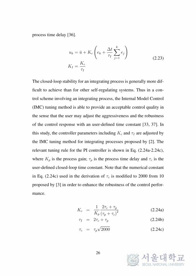
process time delay [36].

uk = u+Kc

(ek +

∆t

τI

k∑j=1

ej

)

KI =Kc

τI

(2.23)

The closed-loop stability for an integrating process is generally more dif-

ficult to achieve than for other self-regulating systems. Thus in a con-

trol scheme involving an integrating process, the Internal Model Control

(IMC) tuning method is able to provide an acceptable control quality in

the sense that the user may adjust the aggressiveness and the robustness

of the control response with an user-defined time constant [33, 37]. In

this study, the controller parameters including Kc and τI are adjusted by

the IMC tuning method for integrating processes proposed by [2]. The

relevant tuning rule for the PI controller is shown in Eq. (2.24a-2.24c),

where Kp is the process gain; τp is the process time delay and τc is the

user-defined closed-loop time constant. Note that the numerical constant

in Eq. (2.24c) used in the derivation of τc is modified to 2000 from 10

proposed by [3] in order to enhance the robustness of the control perfor-

mance.

Kc =1

Kp

2τc + τp

(τp + τc)2 (2.24a)

τI = 2τc + τp (2.24b)

τc = τp√2000 (2.24c)

26

We use a dynamic relative gain array (DRGA) result for configuring the

control loop pairings having a relative gain array (RGA) value close to 1,

which indicates that the intended control loop has strong controllability,

whereas the other configuration does not. DRGA measures the dynamic

interactions within multivariable processes [38], occasionally deriving

more efficient control structures than the steady-state RGA results. [39]

showed in a distillation control problem, that a control configuration with

an infinite steady-state value of the RGA provided a good control effi-

ciency, which was predicted by the high-frequency RGA value close to

1.

First, step inputs and responses on both process outputs shown in

Fig. (6) are fitted into a transfer function in Eq. (2.25) by using ‘tfest’

function in MATLAB 2015a.

PT

=

−2236s+0.4331s2+1.605s+0.004292

9123s+6.868s2+3.289s+0.005147

1.049×104s−0.5323s2+7.635s+0.0008983

−727.9s+1.042s2+4.212s+0.0005245

min

mout

(2.25)

Eq. (2.25) is then plotted against a logscale frequency interval to result

in the DRGA analysis in Fig. (6). The DRGA analysis illustrates that the

acceptable control loop pairings are off-diagonal, which are (P , mout)

and (T , min).

Finally, Kp of the integrating process is determined as the average

value of the response gains by following Eq. (2.26), where ∆u∗ is ∆u

divided by the length of the allowed range of u and ∆y∗ is ∆y divided

by the length of the allowed range of y. The resulting control parameters

27

Figure 6: Step responses and dynamic RGA results of the pre-cooling process;top left: step input trajectories of min and mout, top right: step response tra-jectory of P ; bottom left: step response trajectory of T ; bottom right: dynamicRGA based on Eq. (2.25)

are shown in Table 3 where umax − umax is 0.2 ton/hr for both min and

mout; ymax−ymax for P and T are 900 kPa and 75K, respectively and ∆t

is 0.5h.

∆u∗ =∆u

umax − umin

∆y∗ =∆y

ymax − ymin

Kp =∆y∗

∆t∆u∗

(2.26)

28

Table 3: Control parameters based on [2, 3]

Control loop Kp τp Kc τI KI

(P , mout) -9.042e-4 130 -0.3681 1.176e4 -3.130e-5(T , min) -1.633e-4 220 -1.204 1.990e4 -6.051e-5

2.5 Dynamic simulation results

In this section, the control performances of the discrete MPC and

the PI controller which are illustrated in Sec. 2.4.1 and Sec. 2.4.3, re-

spectively are compared with the proposed pre-cooling process of the

CO2 storage tank. As a result, the MPC control input sequences are influ-

enced by the magnitude of the terminal penalty. Both control algorithms

are able to terminate the process within the designated operation time

limit, however unlike the MPC result, the trajectory of P resulting from

the PI controller experiences significant overshoot well until T reaches

the desired setpoint.

2.5.1 Effect of the weighting matrix Qt on the Lyapunov

stability around the target state xt

Using the initial condition and operational parameters of this system

presented in Table 2, the MPC and the dynamic model is constructed on

the SIMULINK environment in MATLAB R2015a [40, 41]. The effects

of the value of Qt on the size of the region Ω and on the input and output

sequences are considered. The target state xt is chosen as P = 500 kPa,

and T = 243.15K. The initial condition x0 is chosen as P = 300 kPa,

and T = 293.15K. The input constraint U is defined in Eq. (2.27) such

29

that both min and mout have nonnegative values throughout the opera-

tion. The reason that the penalty on offset of T in Q is greater than that

of P comes from the analysis of Eq. (2.14). Whereas dPdt

is less dependent

on T when the tank wall is well insulated, dTdt

is coupled with P . Thus

T should be harder to control than P and therefore its offset is given a

stronger penalty. A slightly greater penalty is on mout because it is desir-

able to have a minimal value of mout. The resulting weighting matrices

Q and R are shown in Eq. (2.28) and the prediction horizon p is set to be

20 steps.

U =

u ∈ R2|u ≥

[0 0

]T(2.27)

Q =

0.2 0

0 1

, R =

0.5 0

0 0.6

(2.28)

To formulate the control problem shown in Eq. (2.18), the Jacobian ma-

trix Φ is obtained by linearizing and discretizing Eq. (2.14) at xt with

∆t = 0.5 h. The eigenvalues in the Eq. (2.29) indicate that the pre-

cooling process example is an integrating process at xt, disabling the

use of the Lyapunov stability condition in Eq. (2.20).

λ (Φ) =[1.0000 0.9930

](2.29)

The stability of xt is confirmed with a gradient plot in Fig. 7. Since xt is a

critical equilibrium, Qt is approximated suboptimally using the modified

Lyapunov stability condition.

30

495 500 505

Pressure [kPa]

242.5

243

243.5

244

Tem

per

ature

[K

]

Figure 7: The gradient plot around the target state P = 500 kPa, T = 243.15K

The interval [−1− λmin (Φ) , 1− λmax (Φ)] is divided into 400 equal

segments, producing 401 different values of κ. Each κ is placed into

Eq. (2.21), excluding the minimum and the maximum points, and yields

Qt. Table 4 shows four cases among these κ and the corresponding eigen-

values of Qt. The region Ω around xt corresponding to the cases in Ta-

Table 4: Change in λ(Qt

)with respect to the change of κ

Case κ λ(Qt

)Case 1 -1.8538 diag(0.7465, 3.8694)Case 2 -1.9235 diag(1.4143, 7.5361)Case 3 -1.9634 diag(3.2663, 18.0846)Case 4 -1.9734 diag(5.0520, 28.6475)

ble 4 is depicted in a purple color in Fig. 8. The size of Ω is the smallest

in Case 1, with Qt also being the smallest. Infeasible regions shown in

a yellow color are present adjacent to xt, except in Case 4, in which no

infeasible region is present. If the state variables exist in the yellow re-

gion, the Lyapunov stability condition becomes infeasible with Qt and

31

the terminal penalty V (xp) diverges. Nevertheless, we know intuitively

that the state trajectories stay inside Ω if they approach xt at the center

in a diagonal direction starting from the upper-left corner where x0 is

located. Therefore V (xp) will remain stable in all four cases.

Figure 8: Change of Ω along the magnitude of Qt; (a) Case 1; (b) Case 2; (c)Case 3; (d) Case 4 (yellow zone: area where Eq. (2.20) is feasible when Qt =Qt; purple zone: area where Eq. (2.20) is infeasible when Qt = Qt)

2.5.2 Effect of Qt on control input and state variable tra-

jectories

The optimal control simulation is calculated using Qt matrices from

Table 4. The resulting input and output sequences are shown in Fig. 9. In

each case, P and T of the storage tank approach the target state rapidly

during the initial phase of the pre-cooling process. Although the converg-

ing speed is reduced thereafter, the calculated input sequence creates an

32

acceptable operation result because the pre-cooling process is completed

within 15 hours, which satisfies the constraint of the operation time.

All four cases of different Qt yield similar mout sequences. The purg-

ing of the CO2 cooling gas through the outlet does not start until t =

2 h (k = 4). At this point, the increasing rate of P is sharply reduced,

whereas the decreasing rate of T is maintained. The cooling power de-

creases as the inlet flowrate of the cooling gas starts to decline afterwards.

A more significant difference is observed in the min sequences. A larger

Qt results in a larger V (xp), reducing the magnitude of state and input

penalty terms in Eq. (2.18). Hence, the initial value of min is larger in

Case 1, resulting in a more stable input sequence than the other cases.

The maximum value of the acceptable cooling rate is approximately

−10K/h. Although a constraint on the rate of change on T or an upper

bound on min is not included in the control objective problem, Fig. 9

shows that the controller satisfies this condition without any constraint

other than Eq. (2.27). An additional constraint may be added to the con-

trol objective problem if the maximum cooling rate exceeds −10K/h at

any time step due to the changes of the operation and control parameters

or the initial condition. In this case the cooling rate can be restricted indi-

rectly by adding an upper bound of u in Eq. (2.27). On the other hand if

the user wants to directly restrict the value of the cooling rate by limiting

the tank temperature T itself, a new type of constraint on the state vari-

able x, e.g. θ ≤ xk+1 − xk is required. This is a time-varying constraint

involving a combination of x and u that reduces the feasible region of the

control objective problem each time when the moving horizon window

33

Figure 9: Dynamic sequences of outputs and control inputs; column 1: controlinputs min and mout; column 2: trajectory of P ; column 3: trajectory of T ; row1: MPC-case 1; row 2: MPC-case 2; row 3: MPC-case 3; row 4: MPC-case 4;row 5: base case-PI control

34

is shifted towards the next time step. Hence, the control objective prob-

lem may become difficult for practical implementations when the state

constraints are imposed.

As the magnitude of min and mout with both control algorithms

reach the minimum values at the end of the operation, we can conclude

that the CO2 BOG formation is restricted with a rigorous application of

controllers, regardless the type of controller. Nevertheless, a noticeable

difference between the results of the MPC application and the PI con-

troller is that the control input sequence of min of the PI controller starts

with a maximum value within the entire trajectory. This is due to the fact

that the PI controller inherently does not take account of the interactions

of P and T which are significantly related to each other when calculating

the feedback control inputs. During the initial operation period when min

is driven to a higher value in order to lower T , P has not yet reached the

required setpoint which delays the opening of mout. Thus P accumulates

inside the tank system until T reaches the setpoint and there is no more

need to retain min above the nominal value.

For small CO2 storage tanks with capacities less than 1500m3, the

tank walls can support pressure around 14–20 bar (1400–2000 kPa) [6].

However the pressure limit tend to decrease to a lesser value as the tank

storage capacities grow. For example, commercial large-capacity storage

tanks for CO2 are operated at a pressure around 5–7 bar (500–700 kPa)

[42]. Although the pressure overshoot occurring during the PI control is

contained within the operation pressure range for the given tank spec-

ification, this phenomenon should be avoided if possible, to secure the

35

overall process stability for various facility operation conditions. Also

despite the initial cooling rate of the PI controller is faster than the MPC,

this is unnecessary since the desirable cooling rate of the pre-cooling

process has been set to −10K/h.

Thus the MPC algorithm shows its effectiveness on the control sta-

bility compared to the PI controller by considering the multivariable in-

teraction when calculating the future control action.

2.5.3 Discussion

In the first part of this case study, a nonlinear dynamic model of the

pre-cooling process required to prevent physical damage to the CO2 stor-

age tank in CO2 carriers is derived from the mass and energy balance

equations of the tank unit. A closed-loop MPC algorithm is developed

with this model to optimize the injection and outlet purge flowrate of

the cooling gas. A terminal penalty is inserted to the objective function

in order to theoretically enhance the state convergence towards the tar-

get setpoint. The second part of this study approximates a suboptimal

weight matrix of the terminal penalty using the modified Lyapunov sta-

bility condition in case the target state equilibrium is not asymptotically

stable. The effect of the weighting matrix of the terminal penalty on the

feasible region around the target state equilibrium and the optimal input

and output sequences are also discussed. Compared to the PI controller

results, the MPC algorithm results show more stability led by the model-

based optimization using the mathematical model. The modeling method

36

and the optimal control provide the pre-cooling process of a CO2 carrier

with an input sequence that reduces the vaporization waste of liquid CO2

cargo and completes the process within the desired operation time limit.

The proposed method calculating a terminal penalty for a dynamic

system handles all eigenvalues equally by indiscriminately ad-

ding an arbitrary constant on them. For a system in which an unstable

eigenvalue is decoupled from other eigenvalues, an improved method

providing the stability and the extra penalty on error accumulations which

are out of range of the control horizon could become a subject of future

studies, so that it can manipulate the problematic eigenvalue separately

from the others and thus handles the issue of instability in a more sophis-

ticated manner.

37

Chapter 3

Concluding remarks

3.1 Summary and contributions

This thesis presents a theoretical approach on designing the geome-

try of a gas cooling system unit and its application with the multivariable

optimal control technique based on the dynamic mathematical models

with a motivation to enhance the cooling efficiency. Two example cool-

ing processes that are discussed in this study and come under this defini-

tion are the CO2 storage tank pre-cooling process and the microparticle

cooling process. Although both processes are included in a same pro-

cess category, the individual process characteristics and their ultimate

goals which need to be achieved are significantly different. Hence, such

factors requiring the main consideration are discussed for the design of

the cooling process units. These apply also on developing the optimal

controller scheme for the gas cooling systems. Rigorous dynamic mod-

elings are derived for each process based on the first principles which

are further used in the development of appropriate model predictive con-

trol (MPC) schemes. The result produced by these optimal controllers

38

are later compared with base cases using the proportional-integral (PI)

controllers, which illustrate that the multivariable optimal control is able

to enhance the stability and the efficiency of both processes. The MPC

schemes applied on each gas cooling systems are formulated with dif-

ferent structures and algorithms. This is because the objectives of both

processes are not same as each other; one aims to reach a far-away target

state with an enhanced penalty on the terminal state-setpoint error, the

other targets to achieve a stable process operation by combining the opti-

mal control algorithm with a PI control loop. Such variation on the con-

trol strategy can be achieved with a thorough study on the first-principle

models, which is difficult to do so by only using the commercial simula-

tors available in the market.

3.2 Suggested future works

Possible subjects for further studies regarding this topic are enlisted

below:

1) A terminal penalty that guarantees the closed-loop stability around the

target equilibrium for a discrete MPC example and has theoretically rig-

orous proofs could provide stronger stability than the terminal penalty

obtained by the modified Lyapunov stability condition, which does not

provide a generalized closed-loop stability. For continuous MPC exam-

ples the method of obtaining a stable terminal penalty has been studied

deeply, but it has been significantly difficult for discrete MPC examples.

2) Scaling-up a process system having turbulent gas flow is hard if the

39

dimensional analysis is not possible. Hence in order to configure a sys-

tem design achieving production objectives in industrial scale, alternative

designing methods should be studied further. First, the user should take

into account of the important physical properties and the characteristics

of fluid mechanics inside the system, possibly using the artificial neu-

ral network (ANN) to configure the relationship between the system ge-

ometry and the fluid flow. Hence some meaningful geometry constraints

could be deduced from this preliminary study. Utilizing this information,

efficiencies of various process designs including the multiple parallel unit

configuration and the single unit setting should be compared with each

other to pick the best scale-up design.

3) An efficient model reduction method not only reduces significant com-

putational power required for the original CFD simulation, but also pro-

vides useful information about the optimal sensor location of a desig-

nated process variable [43]. Model reduction algorithms such as the proper

orthogonal decomposition (POD) using snapshot data or the eigensys-

tems realization algorithm (ERA) [43, 44, 45] have been already stud-

ied in depth in attempt to replace CFD simulation in real-time optimal

control problems or finding efficient sensor locations. To improve the ex-

isting researches, efficient CFD model reduction methods for complex

systems having multiphase flow or chemical reactions could become a

good aim.

40

Bibliography

[1] J.-W. Park, D.-S. Kim, M.-S. Ko, J.-H. Cho, A study on the experimental

measurements and its recovery for the rate of boil-off gas from the storage

tank of the CO2 transport ship, Clean Technology 20 (1) (2014) 1–6.

[2] P. S. Fruehauf, I.-L. Chien, M. D. Lauritsen, Simplified imc-pid tuning

rules, ISA Transactions 33 (1) (1994) 43–59.

[3] B. D. Tyreus, W. L. Luyben, Tuning pi controllers for integrator/dead time

processes, Industrial & Engineering Chemistry Research 31 (11) (1992)

2625–2628.

[4] D. Bjerketvedt, J. R. Bakke, K. Van Wingerden, Gas explosion handbook,

Journal of hazardous materials 52 (1) (1997) 1–150.

[5] A. S. Mujumdar, Handbook of industrial drying, 4th Edition, CRC Press,

2014.

[6] S. G. Lee, G. B. Choi, J. M. Lee, Optimal design and operating conditions

of the CO2 liquefaction process, considering variations in cooling water

temperature, Industrial & Engineering Chemistry Research 54 (51) (2015)

12855–12866.

[7] B. Metz, O. Davidson, H. de Coninck, M. Loos, L. Meyer, Carbon diox-

ide capture and storage: special report of the intergovernmental panel on

climate change, Cambridge University Press, 2005.

[8] B. Y. Yoo, D. K. Choi, H. J. Kim, Y. S. Moon, H. S. Na, S. G. Lee, Devel-

opment of CO2 terminal and CO2 carrier for future commercialized CCS

market, International Journal of Greenhouse Gas Control 12 (2013) 323–

332.

[9] J. Y. Jung, C. Huh, S. G. Kang, Y. Seo, D. Chang, CO2 transport strategy

and its cost estimation for the offshore CCS in korea, Applied Energy 111

(2013) 1054–1060.

41

[10] O. Akhuemonkhan, R. R. Vara, US firm outlines its LNG terminal cool-

down procedure at start-up, LNG Journal (February, 2009) 23–26.

[11] Q. S. Chen, J. Wegrzyn, V. Prasad, Analysis of temperature and pres-

sure changes in liquefied natural gas (LNG) cryogenic tanks, Cryogenics

44 (10) (2004) 701–709.

[12] C. S. Lin, N. T. Van Dresar, M. M. Hasan, Pressure control analysis of

cryogenic storage systems, Journal of Propulsion and Power 20 (3) (2004)

480–485.

[13] Praxair, Praxair cryogenic supply systems: An inside look, 39 Old Ridge-

bury Road, Danbury, CT 06810-5113, USA (2010).

[14] C. Harding, K. Williams, Leak detection and cool-down monitoring at

LNG facilities, in: LNG 17 International Conference, Houston, 2013.

[15] G. Ransom, Pluto LNG plant start-up, in: LNG 17 International Confer-

ence, Houston, 2013.

[16] M.-J. Jung, J. H. Cho, W. Ryu, LNG terminal design feedback from oper-

ator’s practical improvements, in: The 22nd World Gas Congress, Tokyo,

Japan, Citeseer, 2003.

[17] S. J. Qin, T. A. Badgwell, A survey of industrial model predictive control

technology, Control engineering practice 11 (7) (2003) 733–764.

[18] K. den Bakker, A step change in lng operations through advanced process

control, in: 23rd World Gas Conference, Amsterdam, 2006.

[19] H. Michalska, D. Q. Mayne, Robust receding horizon control of con-

strained nonlinear systems, Automatic Control, IEEE Transactions on

38 (11) (1993) 1623–1633.

[20] Y. Yang, J. M. Lee, An iterative optimization approach to design of control

Lyapunov function, Journal of Process Control 22 (1) (2012) 145–155.

[21] F. Dauber, R. Span, Modelling liquefied-natural-gas processes using

highly accurate property models, Applied Energy 97 (2012) 822–827.

42

[22] N. Jang, M. W. Shin, S. H. Choi, E. S. Yoon, Dynamic simulation and

optimization of the operation of boil-off gas compressors in a liquefied

natural gas gasification plant, Korean Journal of Chemical Engineering

28 (5) (2011) 1166–1171.

[23] D. B. Robinson, D. Y. Peng, S. Y. K. Chung, The development of the Peng-

Robinson equation and its application to phase equilibrium in a system

containing methanol, Fluid Phase Equilibria 24 (1) (1985) 25–41.

[24] J. Xiao, Q. Li, D. Cossement, P. Benard, R. Chahine, Lumped parameter

simulation for charge–discharge cycle of cryo-adsorptive hydrogen storage

system, International Journal of Hydrogen Energy 37 (18) (2012) 13400–

13408.

[25] J. M. Smith, H. C. Van Ness, M. M. Abbott, Introduction to chemical en-

gineering thermodynamics, 7th Edition, McGraw-Hill, 2005.

[26] R. Span, W. Wagner, A new equation of state for carbon dioxide covering

the fluid region from the triple-point temperature to 1100K at pressures

up to 800MPa, Journal of Physical and Chemical Reference Data 25 (6)

(1996) 1509–1596.

[27] M. Morari, J. H. Lee, Model predictive control: past, present and future,

Computers & Chemical Engineering 23 (4) (1999) 667–682.

[28] D. Q. Mayne, J. B. Rawlings, C. V. Rao, P. O. Scokaert, Constrained model

predictive control: Stability and optimality, Automatica 36 (6) (2000) 789–

814.

[29] J. B. Rawlings, Tutorial overview of model predictive control, Control Sys-

tems, IEEE 20 (3) (2000) 38–52.

[30] J. H. Lee, M. Morari, C. E. Garcıa, Model Predictive Control, Preprint,

2003.

[31] K. Zhou, J. C. Doyle, K. Glover, et al., Robust and optimal control, Vol. 40,

Prentice hall New Jersey, 1996.

43

[32] P. Shi, E.-K. Boukas, Y. Shi, R. K. Agarwal, Optimal guaranteed cost con-

trol of uncertain discrete time-delay systems, Journal of Computational

and Applied Mathematics 157 (2) (2003) 435–451.

[33] A. Visioli, Q. Zhong, Control of integral processes with dead time,

Springer Science & Business Media, 2010.

[34] H. Chen, F. Allgower, A quasi-infinite horizon nonlinear model predic-

tive control scheme with guaranteed stability, Automatica 34 (10) (1998)

1205–1217.

[35] G. Bitsoris, Positively invariant polyhedral sets of discrete-time linear sys-

tems, International Journal of Control 47 (6) (1988) 1713–1726.

[36] D. E. Seborg, D. A. Mellichamp, T. F. Edgar, F. J. Doyle III, Process dy-

namics and control, 3rd Edition, John Wiley & Sons, 2010.

[37] B. Rice, D. Cooper, Design and tuning of PID controllers for integrating

(non-self regulating) processes, TECHNICAL PAPERS-ISA 422 (2002)

437–448.

[38] Y. A. Husnil, M. Lee, Control structure synthesis for operational optimiza-

tion of mixed refrigerant processes for liquefied natural gas plant, AIChE

Journal 60 (7) (2014) 2428–2441.

[39] S. Skogestad, P. Lundstrom, E. W. Jacobsen, Selecting the best distillation

control configuration, AIChE Journal 36 (5) (1990) 753–764.

[40] L. Wang, Model predictive control system design and implementation us-

ing MATLAB®, Springer Science & Business Media, 2009.

[41] A. Bemporad, M. Morari, N. L. Ricker, Model predictive control toolbox,

user’s guide, The mathworks.

[42] I. GHG, Ship transport of co2, Cheltenham, International Energy Agency

Greenhouse Gas R&D Programme.

[43] B. Apacoglu, A. Paksoy, S. Aradag, CFD analysis and reduced order mod-

eling of uncontrolled and controlled laminar flow over a circular cylinder,

44

Engineering Applications of Computational Fluid Mechanics 5 (1) (2011)

67–82.

[44] S. Hovland, J. Gravdahl, K. Willcox, Explicit MPC for large-scale systems

via model reduction, AIAA Journal of Guidance, Control and Dynamics

31 (4).

[45] K. Li, H. Su, J. Chu, C. Xu, A fast-POD model for simulation and control

of indoor thermal environment of buildings, Building and Environment 60

(2013) 150–157.

45

초록

본논문은기체를제한된공간에주입하여같은공간에유입되

는 외부 열이나 미세입자 형태의 고체 물질의 열을 냉각하는 기체

냉각공정에 대해 다루고 있다. 물 또는 수증기, 에탄올 (ethanol) 을

포함하는휘발성냉매와불소계 (fluorine)물질과달리기체냉각공

정은 질소, 이산화탄소 및 공기와 같은 화학적으로 비활성 상태를

유지하는 유체를 냉매로 사용한다. 이러한 기체들은 냉각 대상의

특성을 보존하는 장점이 있으나 비열이 공기와 같거나 더욱 낮기

때문에실제운전및시스템구조설계단계에서다음과같은문제

가 발생할 수 있다. 1) 냉각 효율이 다른 냉매에 비하여 떨어지기

때문에 시스템을 제외한 기타 물질을 냉각하는 경우 필요한 물질

의체류시간을보장할수있도록냉각시스템의크기를증가시켜야

한다. 2) 낮은 밀도로 인해 같은 조건의 물질 또는 시스템을 냉각

하기위해사용되는유체주입량이많다.이로인한시스템내부의

압력과냉매공급의증가에따른운전및관리비용상승을줄일수

있도록 냉매 주입량을 조절하는 최적 제어 기법을 공정 운전에 적

용해야한다.이에본논문에서는기체냉각공정에포함되는이산화

탄소 (CO2)저장탱크의예냉 (pre-cooling)공정과고분자미세입자

융용 분사 (melt-spray) 공정의 후처리 단계인 냉각기 (spray cooling

chamber)공정을예제로하여공정의용도에부합하는체계적인유

닛 설계 방법과 공정의 동적 모델을 기반으로 하는 다변수 모델예

측제어 (MPC: model predictive control)를적용한안정적인운전전

략을제안하였다.

46

첫 번째 예제인이산화탄소 저장탱크 시스템은 액화 이산화탄

소수송선의부속시설로서,초저온액화이산화탄소를저장주입하

는과정에서발생할수있는탱크벽의열적변형을예방하기위해

탱크 벽면과 내부를 액화 화물과 유사한 온도까지 예냉하는 단계

를 거쳐야 한다. 이 예냉공정은 액화화 이산화탄소 화물의 일부를

기화시켜탱크에주입함으로써탱크내부온도를낮추고압력을상

승시키는과정이다.이산화탄소저장탱크시스템은예냉공정을고

려하지않고선박내선적한계를최대화하는방향에서이낭형 (bi-

lobe)구조의 13 000m3규모로사전설계되었다.예냉공정에대한모

델예측제어의 적용은 탱크에 주입되어야 하는 CO2 기체 주입량을

제한하여 CO2 의 포집 및 액화비용의 손실을 줄이는 효과가 있다.

먼저 공정에 대한 비선형 다변수 동적 모델을 전개하여 CO2 기체

주입유량과배출유량을조절하여탱크내압력과온도를제어하는

수학적관계를정의하였다.이후유한구간선형화모델예측제어기

(finite-horizon linearized MPC)를적용하여예냉공정을제한운전시

간 안에 마무리하는 운전전략을 수립하였다. 적분공정 (integrating

process)인예냉공정의상태변수와설정값 (setpoint)간오차를줄이

고이론적으로유한구간최적화에대한안정성을보장하기위해종

착비용 (terminal penalty)항을목적함수에추가하였다.또한종착비

용은 변형된 리아푸노프 안정성 조건 (Lyapunov stability condition)

의 해로 차선적으로 근사되었다. 종착비용의 가중행렬 (weighting

matrix)은복수의해로계산되며,모델예측제어기의목적함수에관

여하므로계산되는제어입력값과공정출력에영향을주었다.

두 번째 예제인 미세입자 냉각공정 시스템은 미세 고분자입자

융용 분사 (melt-spray) 공정의 후처리 단계인 냉각기 (spray cooling

47

chamber) 를 포함하며, 고온에서 융용 상태로 분사되는 입자와 냉

각용공기를함께냉각기내부로분사,혼합시켜입자를유리화온

도 (Tg: glassification temperature)이하로냉각하여고형화하는공정

이다.이를수행할수있는시스템을제작하기위해먼저냉각기의

구조가 노즐에서 분사되는 구형 미세입자에 충분한 입자체류시간

(PRT: particle residence time)을보장할수있도록이론적인설계기

준을정립하였다.이과정에서입자크기에따라냉각기높이와나

머지 설계 변수들이 입자 냉각에 미치는 영향을 분리하여 평가하

였다. 일차적으로 크기가 상대적으로 큰 입자들에 한하여 노즐에

서 분사된 후 충분한 입자체류시간 (PRT: particle residence time) 을

가지도록 하는 냉각기의 최소 높이를 기존 문헌에 공개된 입자 속

도식과온도식을결합한집중상수모델 (lumped parameter model)을

통해 결정하였다. 냉각기 높이를 결정한 뒤, 냉각기 지름, 하단 원

뿔 높이 및 냉각기 출구 지름에 따라 세분화한 냉각기 구조의 6 개

케이스를지정하였다.크기가상대적으로작은입자의거동은주변

공기의 흐름과 오차가 적으므로, 케이스 별로 고온 공기의 주입유

량이변화한이후의구조내부의공기흐름의변화를전산유체역학

(CFD: computational fluid dynamics)모사를통해계산하는방식으로

크기가작은입자의흐름을간접적으로분석하여냉각기내부공간

에서공기흐름의불안정성이적고,중심부와주변부의공기혼합이

잘이루어지는냉각기구조를 6개케이스중에서선정하였다.최종

적으로결정된냉각기구조내부에서미세입자의냉각이원활하게

이루어짐을 CFD모사로검증하였다.

다음으로 미세입자 냉각공정에 최적제어기를 적용하기 위해

입자상태를실시간으로측정하기어려우므로냉각기내부의공기

48

상태와외부로배출되는공기유량을바탕으로간접적으로냉각효

율을 평가하는 방식을 사용한다. 먼저 냉각공정의 공기 유출입에

대한다변수동적모델링을전개하여냉매로사용되는저온공기와

고온 공기의 유량을 조절하여 냉각기 내부의 공기 온도와 출구를

통해 배출되는 공기 유량을 제어하는 수학적 관계를 정의하였다.

냉각기내부의공기온도는냉각효율과입자생산물의품질을결정

하며, 출구 공기 유량은 냉각기 후속 공정인 입자 포집 및 크기 별

분리 공정의 운전에 영향을 미친다. 따라서 모델예측제어와 비례

적분제어를연결한제어기를도입하여저온공기의사용량을축소

하고, 분사– 냉각– 포집 및 분리로 이어지는 연속공정의 안정적인

운전을유도할수있음을보였다.

주요어 : 예냉공정,미세입자냉각공정,모델예측제어,전산유체역

학

학번 : 2010-21010

49