Optimal control of a wave energy converter*

R. W. M. Hendrikx1, J. Leth2 P. Andersen2 and W. P. M. H. Heemels1

Abstract— The optimal control strategy for a wave energyconverter (WEC) with constraints on the control torque isinvestigated. The goal is to optimize the total energy deliveredto the electricity grid. Using Pontryagin’s maximum principle,the solution is found to be singular-bang. Using higher orderconditions, the optimal control on the singular arc is found asa function of the state and costate trajectories. Furthermore,it is shown that the transitions between bang and singularsubarcs are discontinuous. Based on these findings the resultsof a numerical direct method are validated. Finally, the optimalcontrol is used to benchmark an existing MPC strategy. Itis found that for active control torque constraints the MPCstrategy does not result in the discontinuous singular-bangtransitions. However, the difference in harvested power is small.

I. I NTRODUCTION

Besides well-known clean energy resources such as windand solar energy, the concept of wave energy conversion(WEC) has been studied in Denmark over the past 25 years[1]. WEC represents a variety of methods to extract energyfrom the motion of seawaves, see [2], [3] for a survey. Oneof the methods to convert wave motion into energy is byusing a point absorber. A working prototype of a multiplepoint absorber has been made by the Wave Star company[4]. The point absorber principle uses a float that is attachedto a hinged arm. The motion of the float caused by the waveforces is converted into energy using hydraulic coupling toapower take off (PTO) system (see e.g. [5]). This PTO systemis capable of applying a variable torque to the point absorberarm, such that work is extracted from the wave motion. Thecontrol challenge is to determine this torque signal, such thatthe extracted work, and thereby the energy delivered to thegrid, is maximized.

Various control methods for point absorbers in generalhave been investigated, ranging from simple methods, suchas latching control [6], to more advanced methods, such asMPC [3], [7]. It has been shown in [8] that to optimizework for harmonic wave motion, the PTO system must atcertain time intervals deliver work to the point absorber.This leads to the well-knownreactive control-scheme, inwhich the power is reversed during the reactive part ofthe control strategy, to optimize power production duringthe active part. Furthermore, the optimal control strategy

1Bob Hendrikx and Maurice Heemels are with the ControlSystems Technology Group, Department of Mechanical Engineering,Eindhoven University of Technology, Eindhoven, 5600 MB,The Netherlands r.w.m.hendrikx@student.tue.nl,m.heemels@tue.nl

2John Leth and Palle Andersen are with the Department of ElectronicSystems, Automation & Control, Aalborg University, 9220 Aalborg EastDenmarkjjl,pa@es.aau.dk

without torque constraints has been investigated by Nielsenet al. for irregular sea waves in [9] by using Pontryagin’smaximum principle, leading to a noncausal control strategy.This strategy was modified by Nielsen et al. to obtain animplementable suboptimal strategy.

The system model and control problem presented in thispaper are closely related to what is presented in [10], [11],[12]. However, the cost in [10] includes an interior (state)penalty term and singular solutions are not addressed. In[11] a slightly different control structure is studied for whichno singular solution exists. In [12] the radiation force issimplified yielding a singular-bang solution with an explicitcontrol law given in terms of states only. In this paper theradiation force is expressed as the output of a state spacerealization which, as in [12], also yield a singular-bangsolution but where the control law now depends expliciton costates. Also switching times are determined in [12],whereas transition between singular and bang solutions isaddressed in this paper.

Finally, in [13] an MPC strategy for optimal motion of awave energy converter is studied and compared to theoreticalupper bounds.

For the Wave Star machine, research strategies includingreactive control and MPC have been investigated. The reac-tive control scheme is based on regular wave theory that doesnot include knowledge about future wave torques. Aimingto optimize energy delivered to the grid and also takinginto account losses in the power conversion, Andersen etal. [14] compared this scheme to an MPC strategy. ThisMPC strategy optimizes the harvested energy for a finitehorizon of future predicted wave torques. They showedthat an input-constrained MPC strategy can outperform thereactive controller. A state observer was used to estimate thefuture states of both the system and the wave. This paperaims to derive an open-loop optimal control strategy for alinearized model of the Wave Star point absorber. Both puresine wave excitation forces and realistic measured excitationforces represented by sea states are used. This optimalcontrol strategy will provide insight into the nature of theoptimal control problem and the direction of the power flowin the presence of control torque constraints. Furthermore,the optimal control signal and the resulting energy will beused to assess performance of the MPC strategy derived byAndersen et al.

To solve the optimal control problem, first a linearizedmodel as used in [14] will be obtained. Using this model,the necessary conditions for optimality based on Pontrya-gin’s maximum principle (PMP) will be stated. It will beshown that the nature of the model and the presence of

constraints on the PTO torque will result in the optimalcontrol input containing either bang or singular trajectories,or a combination of both. A characterization of the optimalcontrol on these singular trajectories will be obtained byresorting to higher order conditions. A solution for the casewhere control constraints are not active will be obtainedas a function of initial state and wave excitation force.For the case where constraints are active, we will showthat transitions from bang trajectories to singular trajectorieswill be discontinuous, based on the work of McDanell andPowers [15]. Since it is very difficult to obtain closed formsolutions in the singular-bang case, we will obtain a numericsolution by solving the optimal control problem using adirect approach via the Matlab solver package ICLOCS[16]. The resulting control trajectory will be discussed andcompared to the MPC strategy for different wave profiles.Finally, conclusions will be drawn regarding usefulness ofthe optimal control for real implementation, performance ofthe MPC strategy and possible future research questions.

II. SYSTEM MODEL AND OBJECTIVE FUNCTION

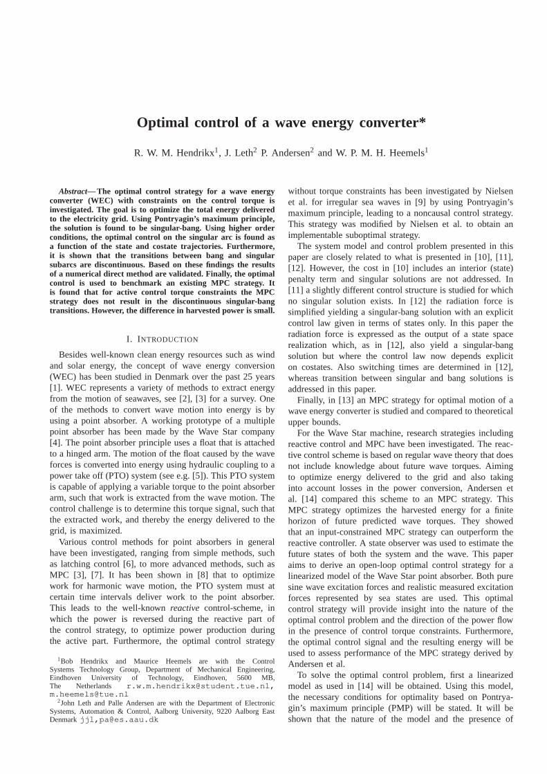
As in [14], a simplified linear model of the point absorberis used. The arm of the point absorber is shown in Figure 1.

Mc

Mhs,Mr,Me

Mean water line

Ja

+

θ

Fig. 1. Schematic depiction of the point absorber model and themomentscaused by water forces and control torque.

We denote the arm angle byθ and the angular velocityand acceleration byω = θ and ω, respectively. The arm ischaracterized by its moment of inertia and the equation ofmotion is given by

Jaω = Mhs+Mr +Me−Mc, (1)

where Mhs denotes the hydrostatic force moment (HsFM),Mr the radiation force moment,Me the external momentcaused by the wave profile andMc the control moment. Forparameter values used in the sequel see Table I below.

The hydrostatic force moment is the moment caused bythe static force of the water pressure on the float with respectto the mean water line (Archimedes’ law). It depends non-linearly on θ , however, a linearized relation is used in [14]of the form

Mhs=−khθ . (2)

The radiation force moment is caused by the forces acting onthe float as it moves through the water, experiencing frictionand water inertia. It is a function ofω and ω and can bedescribed by the relation [17]

Mr =−Jh∞ω −∫ t

0hr(t − τ)ω(τ)dτ , (3)

where the impulse responsehr is determined numerically us-ing a boundary-element method [18]. A transfer function can

then be identified for the convolution part and represented bya state space realization of the form

xr = Arxr +Brω (4a)

Mr = −Jh∞ω +Crxr (4b)

with system matrices (T indicate transpose)

Ar =

0 1 00 0 1

−a0 −a1 −a2

, Br =

001

, Cr =

c1c2c3

T

.

Introducing the moment of inertiaJ= Ja+Jh∞ and combin-ing (1), (2) and (4) yields

ω =−kh

Jθ +

1J

Crxr +1J

Me−1J

Mc (5a)

xr = Arxr +Brω, (5b)

which can be rewritten in state space form

ωωxr

=

0 1 0−kh

J 0 1JCr

0 Br Ar

θωxr

+

0− 1

J0

Mc(t)+

01J0

Me(t), (6)

or more compactly

x(t) = Ax(t)+Bu(t)+Γγ(t), (7)

wherex1 = θ , x2 = ω, xi+2 = xr i , i = 1,2,3, the inputu(t)is used for the control momentMc(t) and the external wavemomentMe(t) is captured in the signalγ(t).

The objective of the optimal control strategy is to maxi-mize the power that is delivered to the grid. To obtain thispower, it is assumed that the arm of the point absorberis connected to an ideal generator through a shaft that isviscously damped. This is shown in Figure 2.

Pc

PG

Mc

ω

bfω MGMc

Fig. 2. Modeling of generator efficiency with friction loss term−bf ω onthe generator shaft. The generated powerPG equals the power flow due tothe control torque (Pc = Mcω) minus the friction power loss.

The (instantaneous) power that is generated equals thepower taken off by the control torquePc = Mcω, minusthe friction power loss (Pf = M f ω), whereM f = bf ω. Thegenerated power,P= PG becomes

P= MGω = Pc−Pf = (Mc−bf ω)ω = uω −bf ω2. (8)

The objective is to maximize the energy delivered to the grid,which is the integral of the powerP. The objective functionthat is to be maximized over a wave sequence of lengtht f

becomes∫ t f

0Pdt=

∫ t f

0

(

u(t)ω(t)−bf ω2(t))

dt. (9)

Where the constraint on the control torque has to be satisfied:

umin ≤ u≤ umax, (10)

with umax = −umin = 2×106 [Nm].

Parameter Value Units DescriptionJa 6.36×106 kgm2 Arm moment of inertiaJ∞ 3.31×106 kgm2 Water moment of inertiakh 29.9×106 Nm/rad HsFM stifnessbf 2.1 Nms/rad PTO friction loss coefficienta0 9.188 - Impulse response parametera1 10.76 - Impulse response parametera2 4.702 - Impulse response parameterc1 6.003×10−4 - Impulse response parameterc2 2.934×107 - Impulse response parameterc3 1.013×107 - Impulse response parameter

TABLE I

PARAMETERS USED IN THE LINEARIZED STATE SPACE MODEL OF THE

POINT ABSORBER.

III. O PTIMAL CONTROL PROBLEM AND PONTRYAGIN’ S

MAXIMUM PRINCIPLE

Using Pontryagin’s maximum principle (PMP) it will beshown that the optimal solution is to either saturate thecontrol (bang) or follow a singular trajectory. Moreover, afeedback expression will be derived for the control on thesingular trajectory and used to obtain the optimal controlfor a case without input constraints. Finally, the behaviorat transitions between singular and bang trajectories willbeanalyzed. The results obtained will be used to validate thenumerical solutions obtained in Section IV.

For given initial conditionx0, external wave momentγ =γ(t) and final timet f , we summarize the optimal controlproblem (in Lagrange form) from Section II:

maxu

∫ t f

0P(x,u)dt, (11a)

subject to the dynamics:

x= Ax+Bu+Γγ , x(0) = x0 (11b)

and the constraint

umin ≤ u≤ umax. (11c)

In the sequel, letu∗ denote a solution to the optimal controlproblem (11), andx∗ the corresponding solution to (11b).Moreover, for a functionf depending onu and/orx we writef ∗ to indicate thatf should be evaluated along the optimalsolutionu∗ and/orx∗.

A. Singular arcs

The Hamiltonian is

H (x,u,λ , t) = P(x,u)+λ T(Ax+Bu+Γγ)

= (x2+λ TB)u−bf x22+λ T(Ax+Γγ)

, Φ(x,λ )u+Θ(x,λ , t), (12)

with switching function (b2 - the second entry inB)

Φ(x,λ ) = x2+b2λ2 (= ω +b2λ2), (13)

andλ ∈ R5 the costate determined by the Cauchy problem

λ =−H∗

x , λ (t f ) = 0

=−ATλ +B1u∗+B2P2x∗, λ (t f ) = 0, (14)

where Hx = ∂H

∂x , P2 is the projection onto the secondcoordinate,B1 =−PT

2 andB2 =−2bf B1.The input that maximizes the Hamiltonian is thus

u=

umax, if Φ∗ > 0

umin, if Φ∗ < 0

singular, if Φ∗ = 0

, (15)

which indicates that the PMP provides no information ifH ∗

u = Φ∗ ≡ 0 on some interval[t1, t2]. If an optimal controlexists on this interval, it is called asingular arc. For thecontrol to be optimal in this case, it is necessary that theGeneralized Legendre-Clebsch(GLC) condition holds [19]:On an optimal singular subarc of orderq, it is necessary that

(−1)q ∂∂u

(

d2q

dt2qH∗

u

)

≤ 0 (16)

where the order of a singular arc is defined as the smallestinteger q, for which the input appears explicitly in theexpression

d2q

dt2qH∗

u =d2q

dt2q Φ∗, (17)

with a coefficient that is not identically zero on[t1, t2].As the∗ notation can be very cumbersome we henceforth

follow common practices and suppress it.

B. Feedback on the singular arc

The control law on a singular arc can be determined bythe demand that the solution must stay on the singular arc(i.e. Hu = Φ = 0 for all t ∈ [t1, t2]) . Hereto we take the timederivatives ofHu until the input appears explicitly. It can beshown that the input only first appears explicitly in the timederivatives for even values ofq (see [15]). We have

Hu = x2+BT λ= P2[Ax+Bu+Γγ(t)]+BT [−ATλ +B1u+B2P2x]

= (P2A+BTB2P2)x−BTATλ +P2Γγ(t) (18)

Hu = (P2A+BTB2P2)(Ax+Bu+Γγ(t))−BTAT(−ATλ +B1u+B2P2x)+P2Γγ(t)

, αu+β (x,λ , t) = 0, (19)

where

α =∂

∂uHu = (P2A+BTB2P2)B−BTATB1. (20)

By substitution of the numerical values in Table I we obtainα = 0.064, verifying that the GLC condition (16) holds (withq= 1). Hence, the input necessary to maintain singularity is

u=−α−1β (x,λ , t), (21)

which, from the definition ofβ , can be written as a linearfeedback in statex, costateλ and external inputsγ , γ

u=−α−1β (x,λ , t), K1x+K2λ +K3γ(t)+K4γ(t), (22)

with (usingu in [MNm])

K1 =[−29.9 92.2 −214.3 −280.3 −52.2], K3 = 1,

K2 =[0 −9.5 0 2.3 −10.8], K4 =−2.3024,

using the values from Table I. Substitution of the feedbacklaw (22) in the system dynamics (11b) and the costatedynamics (14) yields a two-point boundary value problem(TPBVP), where the initial statex0 and the final costateλ (t f ) = 0 are fixed.

For the wave excitation momentγ(t) = 0.4×106sin(t) theMatlab shooting functionbvp4c.m has been used to solvethe TPBVP, resulting in Figure 3. As an indication of cor-rectness, we show the two terms that make up the switchingfunction (13). The coinciding of these terms implies that theresulting trajectory is fully singular.

0 2 4 6 8 10 12 14 16 18

time [s]

-0.2

-0.1

0

0.1

u(t) [×10 MNm]

ω(t) [rad/s]

Power [MW]

−b2λ2

Fig. 3. The trajectories resulting from solving the TPBVP with the shootingalgorithmbvp4c.m.

So far we have been looking at singular solutions only.In general, optimal solutions will consist of both bang andsingular sub-arcs. We now investigate the transition betweenthese two types of sub-arcs.

C. Optimal control at singular-bang junctions

Solving the TPBVP for the optimal control problem (11)is, in general, very difficult since it is not known beforehandat what times the switch between bang and singular arcsshould occur. However, it was shown by McDanell andPowers [15] that ifu is an optimal control containing bothnonsingular subarcs and piecewise continuous,qth ordersingular subarcs, it holds that (superscript indicating orderof time derivative)

(i) If H2q

u 6= 0 on the nonsingular side of a junction, thenthe control is discontinuous.

(ii) If β = 0, α 6= 0 (as defined in (19)) andumin,umax 6= 0at a junction, then the control is discontinuous.

(iii) If u is piecewise continuous on the singular subarc,H

2qu = 0 on the nonsingular side of a junction and

α 6= 0 at the junction, then the control is continuous.

To show that the switching is discontinuous at a junction, wewill show that condition (i) holds without solving the optimalcontrol problem (11) explicitly. In the sequel, we considerexternal wave moments of the formγ = γ sin(at+ φ), seehowever Remark 1 below. These external moments can beregarded as outputs of the exosystem

xe=Aexe, γ =Cexe, Ae=

[

0 1−a2 0

]

, Ce=[

1 0]

,

(23)

for suitable initial conditionxe(0)= (γ sin(φ), γacos(φ)). Weadd the exosystem to the system dynamics (11b), to form thewave-autonomous system(A, B)

˙x= Ax+ Bu, A=

[

A ΓCe

0 Ae

]

, B=

[

B0

]

. (24)

For this system we can again form the Hamiltonian, in away similar to (12), where the explicit inputγ(t) is nowleft out as it is generated within the system itself. Extendingthe matricesB1,B2,P2 used in (19) with two zero entries toaccount for the new state ˜x∈ R

7, we obtain the following

Hu = (P2AA− BT ATB2P2+ BTB2P2A)x+ BT AT AT λ+(P2AB− BT ATB1+ BTB2P2B)u= 0 (25)

which is equivalent to (19), without the terms containingγ , γ.Introducing the augmented state ˜z=

[

xT λ T]T

, we canwrite (25) as

mT z= k, (26)

where

m=∂∂ z

Hu, k=−∂∂u

Huu=−αu, (27)

a row vector and scalar, respectively, defined by (25). Thedynamics that ˜z must satisfy are given by

˙x = Ax+ Bu (28)

˙λ = −∂H

∂ x=−ATλ +B1u+B2P2x. (29)

We write this as˙z= F z+ g, (30)

whereF =

[

A 0B2P2 −AT

]

, g=

[

BB1

]

u. (31)

To verify condition (i) forHu we assume that ˜g is a constantinput since in this case the local optimal control satisfies oneof the active constraints, i.e.u= ubang∈ {umin,umax}.

Now employ the state transformation

ζ = z+ F−1g, (32)

transforming (30) to a homogeneous system on a nonsingularsubarc. Applying this transformation to the affine state con-straint expressed by (26) as well, we obtain the expression

mTζ = k+mT F−1g. (33)

We show that the right-hand side of this expression is zeroby observing that

F−1 =

[

A−1 0

A−TB2P2A−1 −A−T

]

, (34)

leading to

mT F−1g=[

P2AB+ BTB2P2B− BT ATB1]

u, (35)

which equals−k (see (25)), thus canceling the expressionfor k in the right-hand side of (33). As a result, to showthat condition (i) is satisfied for the optimal control problem

under consideration, it suffices to show that there exists nointerval [t1, t2] on the nonsingular side of a junction where

ζ = Fζ , mTζ = 0, (36)

for any allowable stateζ (t1) = ζt1 6= 0. Hence, it is enoughto show that the set of allowable states are unobservable withrespect to the pair(F ,mT). That is, a sufficient condition for(36) to have no solution is that

Z ∩U O =∅ (37)

with the set of allowable states

Z = {ζ ∈ R14|Lζ 6= 0}, L =

[

02×5 I2×2 02×7]

, (38)

and the unobservable subspace

U O = {ζ ∈ R14|Oζ = 0}, O=

mT

mT F...

mT Fn−1

. (39)

Using the values in Table I , a basis for the (2-dimensional)unobservable subspace is obtained1

U O = Range

{[

012×2

I2×2

]}

, (40)

implying that (37) holds true. Thus there can exist no interval[t1, t2] on whichHu ≡ 0, and therefore the transition betweenbang and singular subarcs of the optimal input must bediscontinuous.

Remark 1:We only showed discontinuous transitions inthe case of external wave moments on the form (23). How-ever, the result can be extended to more general classes ofexternal waves e.g., those composed by sinusoids, with theuse of

AE = diag(Ae, . . . ,Ae), CE =[

Ce · · · Ce]

,

xE(0) = (γ1sin(φ1), γ1a1cos(φ1), . . . , γk sin(φk), γkak cos(φk)).

A further analysis of the switching times between bang andsingular sub-arcs will be conducted in future work. However,the above will be used to verify that the numerical solutionsobtained in the next section have the correct qualitativebehavior (see e.g. [20], [21] for a discussion on methodsfor numerical solution of optimal control problems).

IV. SOLUTIONS FROM THE DIRECT METHOD

In this section, we use a different approach from theone used in Section III. Thedirect method, also known asthe first-discretize-then-optimizemethod, poses the optimalcontrol problem as a non-linear optimization problem inthe time-discretized state and input space. Multiple softwarepackages and manual methods exist for this method (see[21]). We chose the free solver package ICLOCS [22], sinceit produced the most accurate results out of several options.ICLOCS is a direct solving package that uses the trapezoidal

1The unobservable modes of the system originate from the costatedynamics−AT in F that contain a copy of the exosystem dynamicsAe.

collocation method2 in which the optimal control problem isdivided into multiple intervals that are solved separately. Ituses the third-party CVODE ODE solver, with anAdamsimplicit integrationscheme andNewton iterationto generatea non-linear program. This NLP is then solved by a third-party NLP solver. ICLOCS allows the usage of both Matlab’sfmincon.m and the third party open source solver IPOPT.

A. ICLOCS output comparison for different NLP solvers

We run a simulation for 10π seconds for an externalwave momentγ = 2sin(t) [MNm] and the resulting input isshown in Figure 4. We used both the IPOPT solver and thefmincon.m solver and found that both result in differentcontrol trajectories. It can be seen in Figure 4 that with theIPOPT solver we see a jump discontinuity (blue) at singular-bang junctions, whereas with thefmincon.m solver thetransition appears continuous. Furthermore, since ICLOCSuses aninfeasible-pathapproach (see [23]), Lagrange mul-tipliers are available for the dynamic constraints (11b).These multipliers are the discrete equivalent of the costatetrajectories that appear in the indirect method and allow tocheck if the necessary conditions obtained in Section IIIhold. The singular input (red) introduced in (21) is shownas a function of the state and the Lagrange multipliers. Itcoincides perfectly with the singular interval for the IPOPTsolver. For thefmincon.m this is not the case. This stronglysuggests that the IPOPT output is the correct optimal control.

0 5 10 15 20 25 30

-3

-2

-1

0

1

2

3

ICLOCS output with IPOPT solveruact [MNm]using = −α−1β(x,λ, t)

time [s]0 5 10 15 20 25 30

-3

-2

-1

0

1

2

3

ICLOCS output with FMINCON solveruact [MNm]using = −α−1β(x,λ, t)

Fig. 4. The optimal control problem solved by ICLOCS with boththeIPOPT and FMINCON solver. The singular input is also shown asa functionof the state and Lagrange multipliers.

B. Optimal control strategy

In Figure 5 the relevant state trajectories are shown. Theterms b2λ2 and ω that form the switching functionΦ arealso shown to verify the position of the singular arcs thatshould appear wheneverΦ = 0. The intervals where theseterms coincide are clearly visible, again confirming thatthe results are as we would expect. Figure 6 shows thetrajectories ofHu, that are zero on the singular interval aswe would expect. Furthermore, the values ofβ (γ ,λ , t) areshown. Interestingly, the sufficient condition (ii) discussed

2We stress that, while this is an advanced method aiming to solvethecontinuous time control problem, the MPC method explained in Section Vaddress a sampled control system constraining the control signal to beconstant between sampling instants.

0 5 10 15 20 25 30

time [s]

-0.2

-0.1

0

0.1

0.2

θ [rad] ω [rad/s] −b2λ2 Me [×10 MNm]

Fig. 5. The controlled response of the statesθ andω to an external wavemomentMe = γ = 2sin(t). The termsb2λ2 and ω that form the switchingfunction Φ are added to show that the singular intervals of the controlcoincide perfectly with the intervals whereΦ = 0.

in Section III-C does not hold, as can be clearly seen fromthe first singular arc in the plot. Understanding the optimal

0 5 10 15 20 25 30

time [s]

-0.4

-0.2

0

0.2

0.4

Hu

β(x,λ, t)

Fig. 6. Plots of the trajectories ofHu that is zero on the singular intervalsandβ that is non-zero both before and on the singular intervals.

control strategy, and especially the discontinuous behavioron junctions, is a nontrivial task since the dynamics of thepoint absorber are complicated. We recall that for power tobe delivered to the grid, the sign ofu must be equal to thesign ofω. We would expect that the optimal control solutionis to keep the signs equal. Figure 7 shows the power that isdelivered to the grid. Clearly, in the optimal solution thereare times when power is reversed and the grid is poweringthe point absorber. These power reversals occur whenevera switch to a singular arc occurs. The control switchesdiscontinuously to approximately zero and the friction termsbecome dominant. After some time on the singular arc thecontrol crosses a point where the angular velocity stayspositive (resp. negative) and the torque becomes positive(resp. negative) again, leading to a short time of zero power.The discontinuous transition to the saturated control thenagain results in a short interval of power loss. It appearsthat this strategy, while suboptimal locally, optimizes futureenergy harvest. This result is in line with the findings ofprevious research, that the optimal strategy is to reversepower at certain times.

0 5 10 15 20 25 30

time [s]

-0.1

0

0.1

0.2

P [MW]

Fig. 7. The power that is generated using the optimal control torque.During the singular intervals, the generated power switches discontinuouslyto a singular arc in order to minimize the energy loss that is necessary formaximizing future energy harvest.

V. COMPARISON WITH MPC STRATEGY

In this section, we will compare the optimal control solu-tion to the MPC control solution derived by Andersen et al.in [14]. The MPC strategy uses a zero-order-hold discretizedversion of the system dynamics (11b), with sample time

τmpc = 0.1s. The optimal input sequence is calculated fora horizon ofTmpc = 8s, with N = Tmpc/τmpc, and the firstinput is implemented at each time instantt = kτmpc for k∈N,leading to

uk = argmax

[

τmpc

k+N−1

∑ℓ=k

ωℓ+1uℓ−bf ω2ℓ+1

]

, (41)

subject to (forℓ= k, . . . ,k+N−1)

xℓ+1 = Adxℓ+Bduℓ+Γdγℓ, umin ≤ uℓ ≤ umax. (42)

Where (41) is a discretized approximation of the energy gen-erated and (42) are the discretized wave converter dynamicsand the control torque constraints. The constraint optimiza-tion problem is solved for sampled time series of externalwave momentsγk, using the Matlab routinequadprog.m.In [14], Andersen et al. used a Kalman filter for estimatingthe state of the system dynamics and a wave generatingmodel. However, wave estimation is beyond the scope ofthis paper and we will remove this model for the purposeof comparison. We will assume that the MPC strategy isaware of the actual wave sequence. This will make it morestraightforward to find the qualitative differences between theoptimal and MPC strategy.

A. Excitation moments

The three external wave moments that are used are shownin Figure 8. Two perfect sinewaves are used, whereMe1

will have singular-bang optimal solution andMe2 will havea totally singular solution where no constraints are active.Furthermore,Me3 will consist of wave moments, generatedusing a stochastic Pierson-Moskowitz spectrum model, clas-sified as sea stateS3 as used in [14]. To reduce computationalefforts, the sea state is shortened (compared to [14]) and allthree wave moments will have a total simulation time of 50seconds (compared to 650 seconds in [14]).

0 5 10 15 20 25 30 35 40 45 50

time [s]

-4

-2

0

2

4

Mom

ent[M

Nm] Me1 = 2 sin(t) Me2 = 0.5 sin(t) Me3, S3 state

Fig. 8. Wave excitation moments that were used to compare the MPCstrategy with the optimal strategy.

B. Comparison method

The average power generated in the MPC simulation iscalculated by Andersen et al. using a discrete approximation:

Wdiscr = τmpc

N−1

∑k=0

ωk+1uk−bf ω2k+1, (43)

Pdiscr = Wdiscr/Tmpc. (44)

To compare the results from the optimal control simulationsand the MPC simulations, we must account for the fact

that the energy determined by ICLOCS is more precisethan this discrete approximation. Therefore, after runningthe total MPC simulation and obtaining the MPC input,we re-simulate the model response to the MPC input usingode45.m, assuming that the input is applied using zero-order hold. The cost is now integrated as an extra state,relying on the higher order integration ofode45.m toproduce more accurate results. In the next section, we willpresent both the discrete power and thecontinuouspowerresulting from the re-simulation usingode45.m.

C. Comparison results

The results of the comparison are shown in Table II. Thepower that was produced by the optimal control input isshown in the right column. The first two columns show thepower calculated as in (44), and simulated as an extra stateusing ode45.m, respectively. The numbers in parenthesescorrespond to the first 38 seconds, approximately corre-sponding to the last time a wave (Me1 or Me2) has completeda full period without entering the last 8 seconds where theMPC horizon looks beyond the total simulation time of 50seconds.

It can be seen that in all cases the MPC strategy performsvery well and is able to harvest close to maximum energy.The relative MPC performance for the low amplitude ex-ternal waveMe2 is 92% (86%). For the waves with higheramplitude we see that the MPC is able to harvest 98% (99%)of the optimal energy. This difference might be explained bythe active constraints in the latter cases. With large regionsof active constraints, the problem reduces to determining theright switching times. Whereas for the case with singularcontrol, the strategy leaves more room for deviations fromthe optimal strategy. We do note however, that these resultsuse the exact same model for the MPC and the simulation.Furthermore, the MPC has full knowledge of future wavemoments. Therefore these results cannot be translated to areal wave machine. They serve merely to validate the MPCoptimization approach.

MPC, discr. MPC, ode45. Optimal

Me1 Sine, ampl. 2 60.1 (57.1) 64.5 (61.4) 65.8 (61.9)Me2 Sine, ampl. 0.5 3.92 (3.52) 4.61 (4.28) 5.03 (4.95)

Me3 Sea state S3 43.4 (42.6) 46.0 (45.5) 46.8 (46)

TABLE II

AVERAGE PRODUCED POWER(IN [KW]) FOR THE DIFFERENT EXTERNAL

WAVE MOMENTS AND THE DIFFERENT CONTROL INPUTS(PAVG =W/T)

(MPC ODE45 CONTAINS THE ODE45SIMULATED COST RESULTING

FROM THE SAMPLEDMPC INPUT)

Figure 9 shows the state, input and power trajectoriesfor the wave momentMe1. The MPC input is plotted as astaircase, as it is applied in this way. It can be seen that theMPC strategy and the optimal strategy are quite similar. Themain difference is in the singular arcs, where the MPC doesnot show the discontinuous behavior (it resembles behaviorsimilar to the fmincon plot in Figure 4). This results in a

different power flow in these regions. Figure 10 shows thesame behaviour. The parts where constraints are active co-incide, however the control strategy differs when constraintsare not active. The reason for this is not clear, although wesuspect that it has to do with either the discrete cost functionapproximation that is not exact, or the solver not findingthe global maximum. We saw similar results when using adifferent NLP solver for the optimal control in Section IV-A that also failed to capture this discontinuity. Althoughthe result is interesting and deserves further attention, theimpact on produced power is small. The difference we seein power production can most likely be contributed to theshorter horizon of the MPC strategy.

0 5 10 15 20 25 30 35 40 45 50

time [s]

-0.1

0

0.1

0.2

ang.vel.[rad/s] ω, MPC ω, optimal

0 5 10 15 20 25 30 35 40 45 50

time [s]

-2

0

2Moment[M

Nm]

u, MPC u, optimal

0 5 10 15 20 25 30 35 40 45 50

time [s]

-0.1

0

0.1

0.2

Pow

er[M

W] PG, MPC PG, optimal

Fig. 9. Angular velocity reponse, control moment and generated powerfor the external wave momentMe1 (A perfect sine with an amplitude of 2[MNm]). The resulting input contains both singular and bang arcs.

0 5 10 15 20 25 30 35 40 45 50

time [s]

-0.2

0

0.2

ang.vel.[rad/s]

ω, MPC ω, optimal

0 5 10 15 20 25 30 35 40 45 50

time [s]

-2

0

2

Moment[M

Nm] u, MPC u, optimal

0 5 10 15 20 25 30 35 40 45 50

time [s]

-0.1

0

0.1

0.2

Pow

er[M

W] PG, MPC PG, optimal

Fig. 10. Angular velocity response, control moment and generated powerfor the external wave momentMe3 (Measured sea state S3). The resultinginput contains both singular and bang arcs.

In Figure 11 we show the simulation results for the exter-nal wave momentMe2. This wave moment was used becauseit results in inactive constraints. It was found numericallyimpossible to completely remove the constraints for theoptimal control simulation with ICLOCS. We see that theoptimal control briefly touches a constraint and results ina sine wave with a constant torque shift. Apart from thisshift, the resulting control strategies from the MPC andoptimal simulation appear quite similar. Interestingly, MPCdoes result in a zero-mean torque. As one would physicallyexpect, a static torque shift does not greatly influence thetotal energy generated, which also is illustrated in Figure11.The qualitative difference in the MPC and optimal controlmay likely be contributed to the discretization and the shorterprediction horizon.

0 5 10 15 20 25 30 35 40 45 50

time [s]

-0.1

0

0.1

ang.vel.[rad/s]

ω, MPC ω, optimal

0 5 10 15 20 25 30 35 40 45 50

time [s]

-2

0

2

Moment[M

Nm]

u, MPC u, optimal

0 5 10 15 20 25 30 35 40 45 50

time [s]

-0.05

0

0.05

0.1

Pow

er[M

W] PG, MPC PG, optimal

time [s]0 5 10 15 20 25 30 35 40 45 50

Energy

[MJ]

-0.1

0

0.1

0.2EG, MPC EG, optimal

Fig. 11. Angular velocity response, control moment, generated power andenergy for the external wave momentMe2 (A perfect sine with an amplitudeof 0.5 [MNm]). The resulting input is totally singular.

VI. CONCLUSIONS

In this paper, we investigated the optimal control strategyof a wave energy converter in the presence of control torqueconstraints. We used a linearized model of the wave energyconverter dynamics and implemented power take off frictionloss in the harvested energy integral. We showed usingPontryagin’s maximum principle that the optimal solution issingular-bang. To obtain a characterization of the singularsolution we used higher order derivatives of the switch-ing function and verified the result using the GeneralizedLegendre-Clebsch condition. We showed that the transitionsfrom bang to singular subarcs are discontinuous. For this pur-pose, we used a state transformation to prove non-zeronessof the second time derivative of the switching function,reducing it to a simple observability test. We used thesefindings to verify the result of a numerical direct method.It was found that the numerical direct method was sensitiveto the choice of NLP solver. The characterization of thesingular solution and the proof of discontinuous singular-bang transitions validated that the numerical results arecorrect. It was found that the optimal control strategy inthe presence of control torque constraint reverses power atcertain intervals to optimize the total energy that is harvested.This is in line with the results for unconstrained optimalcontrol found in literature.

The optimal control was used to validate an existingMPC strategy. It was found that the MPC strategy exhibitsqualitatively different singular behavior than the optimalcontrol. The impact of this difference on energy productionwas determined for various wave signals and was found to besmall. The MPC strategy performs very well and in all casesharvests at least 92% (86%) of the energy. The differencebetween the optimal control and the MPC strategy is mostlikely due to the discretization of the cost function, or thesolver failing to find the global optimum. More researchis needed to give definitive conclusions. However, we canstate that the optimal control problem for the linearized

system with active constraints can be accurately solved.The MPC strategy shows performance close to this optimalcontrol strategy and is therefore a very valid candidatefor implementation. For practical purposes, future researchshould focus on more accurate models of the wave energyconverter and the power take off friction. For theoreticalpurposes, the cause of the difference in singular behaviormay be interesting. Furthermore, a challenge may lie indetermining numerically reliable totally singular solutionsfrom Pontryagin’s principle, and translating these solutionsto practically implementable control strategies.

REFERENCES

[1] J. Kofoed, P. Frigaard, and M. Kramer, “Recent developments onwave energy utilization in Denmark,”Proceedings of the Workshopon Renewable Ocean Energy Utilization, 2006.

[2] A. M utze and J. Vining, “Ocean wave energy conversion, a survey,”Proceedings of the 41st IEEE IAS Annual Conference, vol. 3, pp.1410–1417, 2006.

[3] J. Ringwood, G. Bacelli, and F. Fucso, “Energy-maximizingcontrolof wave-energy converters,”IEEE control systems magazine, vol. 34,no. 5, 2014.

[4] Wave Star A/S, “http://www.wavestarenergy.com.”[5] R. Hansen, T. Andersen, and H. Pedersen, “Model based design of

efficient power take-off systems for wave energy converters,” TheTwelfth Scandinavian International Conference on Fluid Power, 2011.

[6] Z. Feng and E. C. Kerrigan, “Latching declutching control of wave en-ergy converters using derivative-free optimization,”IEEE Transactionson Sustainable Energy, vol. 6, no. 3, pp. 773 – 780, 2015.

[7] J. Barradas-Berglindet al., “Energy capture optimization for an adap-tive wave energy converter,” inProceedings of the 2nd InternationalConference on Renewable Energies Offshore - RENEW 2016, 2016.

[8] J. Falnes, “Optimum control of oscillation of wave-energy converters,”International Journal of Offshore and Polar Engineering, 2002.

[9] S. Nielsen, Q. Qiang, M. Kramer, B. Basu, and Z. Zhang., “Optimalcontrol of non-linear wave energy point converters,”Ocean engineer-ing, vol. 72, no. 11, 2013.

[10] G. Li, G. Weiss, M. Mueller, S. Townley, and M. R. Belmont,“Wave energy converter control by wave prediction and dynamicprogramming,”Renewable Energy, vol. 48, pp. 392 – 403, 2012.

[11] E. Abraham and E. C. Kerrigan, “Optimal active control and optimiza-tion of a wave energy converter,”IEEE Transactions on SustainableEnergy, vol. 4, no. 2, pp. 324 – 332, 2013.

[12] S. Zou, O. Abdelkhalik, R. Robinett, G. Bacelli, and D. Wilson,“Optimal control of wave energy converters,”Renewable Energy, vol.103, pp. 217 – 225, 2017.

[13] J. Hals, J. Falnes, and T. Moan, “Constrained optimal control of aheaving buoy wave-energy converter,”Journal of Offshore Mechanicsand Arctic Engineering, ASME, vol. 133, February 2011.

[14] P. Andersen, T. S. Pedersen, K. M. Nielsen, and E. Vidal,“Modelpredictive control of a wave energy converter,”IEEE Conference onControl Applications, pp. 1540–1545, 2015.

[15] J. Mcdanell and W. Powers, “Necessary conditions for joining optimalsingular and nonsingular subarcs,”Siam Journal of Control, vol. 9,no. 2, 1971.

[16] P. Falugi, E. Kerrigan, and E. V. Wyk, “ICLOCS,” 2010. [Online].Available: http://www.ee.ic.ac.uk/ICLOCS

[17] W. Cummins, “The impulse response function and ship motions,”Schiffstechnick, 1962.

[18] Wamit user manual, Wamit inc., Chestnut Hill, MA, 2002.[19] H. J. Kelley, R. E. Kopp, and H. G. Moyer, “Singular extremals,” in

Topics in Optimization. Academic Press, 1967, pp. 63–101.[20] O. von Stryk and R. Bulirsch, “Direct and indirect methods for

trajectory optimization,”Annals of Operations Research, vol. 37, 1992.[21] A. Rao, “A survey of numerical methods for optimal control,” Ad-

vances in the astronautical Sciences, vol. 135, no. 1, 2010.[22] B. Houska, H. Ferreau, and M. Diehl, “ACADO Toolkit – An Open

Source Framework for Automatic Control and Dynamic Optimization,”Optimal Control Applications and Methods, vol. 32, no. 3, pp. 298–312, 2011.

[23] M. Diehl, “Lecture notes on optimal control and estimation,” 2014.