Embed Size (px)
Citation preview

Lecture – 25
Optimal Control Formulation using Calculus of Variations
Dr. Radhakant PadhiAsst. Professor
Dept. of Aerospace EngineeringIndian Institute of Science - Bangalore

ADVANCED CONTROL SYSTEM DESIGN Dr. Radhakant Padhi, AE Dept., IISc-Bangalore
2
TopicsOptimal Control Formulation
• Objective & Selection of Performance Index
• Necessary Conditions of Optimality and Two-Point Boundary Value Problem (TPBVP) Formulation
• Boundary/Transversality Conditions
• Numerical Examples

Optimal Control Formulation:Objective & Selection of Performance Index
Dr. Radhakant PadhiAsst. Professor
Dept. of Aerospace EngineeringIndian Institute of Science - Bangalore

ADVANCED CONTROL SYSTEM DESIGN Dr. Radhakant Padhi, AE Dept., IISc-Bangalore
4
Objective
( )
( )
0To find an "admissible" time history of control variable , , which:
1) Causes the system giverned by , , to follow an admissible trajectory
2) Optimizes (minimizes/maximizes)
fU t t t t
X f t X U
⎡ ⎤∈ ⎣ ⎦
=
( ) ( )
( )
0
0 0
a "meanigful" performance index
, , ,
3) Forces the system to satisfy "proper boundary conditions". [ our focus: (given), : fixed ]
ft
f ft
f
J t X L t X U dt
X t X t
ϕ= +
=
∫

ADVANCED CONTROL SYSTEM DESIGN Dr. Radhakant Padhi, AE Dept., IISc-Bangalore
5
Meaningful Performance Index
( ) [ ]0
0
0
1) Minimize the operational time
1 0, 1
2) Minimize the control effort
1 1, 0 0,2 2
3) Minimize deviation of state from a fixed value with minimum co
f
f
t
ft
tT T
t
J t t dt L
J U RU dt R L U RU
C
ϕ
ϕ
= − = = =
⎡ ⎤= > = =⎢ ⎥⎣ ⎦
∫
∫
( ) ( )0
ntrol effort
1 , 0, 02
ftT T
t
J X C Q X C U RU dt Q R⎡ ⎤= − − + ≥ >⎣ ⎦∫

ADVANCED CONTROL SYSTEM DESIGN Dr. Radhakant Padhi, AE Dept., IISc-Bangalore
6
Meaningful Performance Index
0
4) Minimize deviation of state from origin with minimum control effort
1 , 0, 02
5) Minimize the control effort, while the final state
reaches close to a constant
ftT T
t
f
J X QX U RU dt Q R
X
C
⎡ ⎤= + ≥ >⎣ ⎦∫
( ) ( ) ( )0
1 1 , 0, 02 2
ftT T
f f f ft
J X C S X C U RU dt S R= − − + ≥ >∫

Optimal Control Using Calculus of Variations: Hamiltonian Formulation
Dr. Radhakant PadhiAsst. Professor
Dept. of Aerospace EngineeringIndian Institute of Science - Bangalore

ADVANCED CONTROL SYSTEM DESIGN Dr. Radhakant Padhi, AE Dept., IISc-Bangalore
8
Optimal Control Problem
Performance Index (to minimize / maximize):
Path Constraint:
Boundary Conditions:
( ) ( )0
, , ,ft
f ft
J t X L t X U dtϕ= + ∫
( ), ,X f t X U=
( )( )
00 :Specified
: Fixed, : Freef f
X X
t X t
=

ADVANCED CONTROL SYSTEM DESIGN Dr. Radhakant Padhi, AE Dept., IISc-Bangalore
9
Necessary Conditions of Optimality
Augmented PI
Hamiltonian
First Variation
( )0
ftT
t
J L f X dtϕ λ⎡ ⎤= + + −⎣ ⎦∫( )TH L fλ+
( )
( )0
0
f
f
tT
t
tT
t
J H X dt
H X dt
δ δϕ δ λ
δϕ δ λ
= + −
= + −
∫
∫

ADVANCED CONTROL SYSTEM DESIGN Dr. Radhakant Padhi, AE Dept., IISc-Bangalore
10
Necessary Conditions of Optimality
First Variation
Individual terms
( )0
ftT T
t
J H X X dtδ δϕ δ δλ λ δ= + − −∫
( ) ( ),T
f f ff
t X XXϕδϕ δ
⎛ ⎞∂= ⎜ ⎟⎜ ⎟∂⎝ ⎠
( ) ( ) ( ) ( ), , , T T TH H HH t X U X UX U
δ λ δ δ δλλ
∂ ∂ ∂⎛ ⎞ ⎛ ⎞ ⎛ ⎞= + +⎜ ⎟ ⎜ ⎟ ⎜ ⎟∂ ∂ ∂⎝ ⎠ ⎝ ⎠ ⎝ ⎠

ADVANCED CONTROL SYSTEM DESIGN Dr. Radhakant Padhi, AE Dept., IISc-Bangalore
11
Necessary Conditions of Optimality
( ) ( )
( )
( )
0 0
0 00
0
0
,
,
0 0
f f
ff f
f
f
t tT T
t t
t Tt XT
t Xt
tTT T T
f ft
tTT T
f ft
d XX dt dt
dt
dX X dtdt
X X X dt
X X dt
δ
δ
δλ δ λ
λλ δ δ
λ δ λ δ δ λ
λ δ δ λ
⎛ ⎞= ⎜ ⎟
⎝ ⎠
⎛ ⎞⎡ ⎤= − ⎜ ⎟⎣ ⎦ ⎝ ⎠
⎡ ⎤= − −⎣ ⎦
= −
∫ ∫
∫
∫
∫
0

ADVANCED CONTROL SYSTEM DESIGN Dr. Radhakant Padhi, AE Dept., IISc-Bangalore
12
Necessary Conditions of Optimality
First Variation
( ) ( )
( ) ( ) ( )
( ) ( )
0
0 0
f
f f
T T
f f ff
tT T T
t
t tT T
t t
J X XX
H H HX U dtX U
X dt X dt
ϕδ δ δ λ
δ δ δλλ
δ λ δλ
⎛ ⎞∂= −⎜ ⎟⎜ ⎟∂⎝ ⎠
⎡ ∂ ∂ ∂ ⎤⎛ ⎞ ⎛ ⎞ ⎛ ⎞+ + +⎜ ⎟ ⎜ ⎟ ⎜ ⎟⎢ ⎥∂ ∂ ∂⎝ ⎠ ⎝ ⎠ ⎝ ⎠⎣ ⎦
+ −
∫
∫ ∫
ADVANCED CONTROL SYSTEM DESIGN Dr. Radhakant Padhi, AE Dept., IISc-Bangalore
13
Necessary Conditions of Optimality
First Variation
( )
( ) ( )
( )
0 0
0
f f
f
T
f ff
t tT T
t t
tT
t
J XX
H HX dt U dtX U
H X dt
ϕδ δ λ
δ λ δ
δλλ
⎡ ⎤∂= −⎢ ⎥
∂⎢ ⎥⎣ ⎦
∂ ∂⎡ ⎤ ⎡ ⎤+ + +⎢ ⎥ ⎢ ⎥∂ ∂⎣ ⎦ ⎣ ⎦
∂⎡ ⎤+ −⎢ ⎥∂⎣ ⎦
∫ ∫
∫= 0

ADVANCED CONTROL SYSTEM DESIGN Dr. Radhakant Padhi, AE Dept., IISc-Bangalore
14
Necessary Conditions of Optimality: Summary
State Equation
Costate Equation
Optimal Control Equation
Boundary Condition
( ), ,HX f t X Uλ
∂= =∂
HX
λ ∂⎛ ⎞= −⎜ ⎟∂⎝ ⎠
0HU∂
=∂
ffX
ϕλ ∂=∂
( )0 0 : FixedX t X=

ADVANCED CONTROL SYSTEM DESIGN Dr. Radhakant Padhi, AE Dept., IISc-Bangalore
15
Necessary Conditions of Optimality: Some CommentsState and Costate equations are dynamic equationsOptimal control equation is a stationary equationBoundary conditions are split: it leads to Two-Point-Boundary-Value Problem (TPBVP)State equation develops forward whereas Costate equation develops backwardsTraditionally, TPBVPs demand computationally-intensive iterative numerical proceduresThese iterative numerical procedures lead to “open-loop” control solutions

ADVANCED CONTROL SYSTEM DESIGN Dr. Radhakant Padhi, AE Dept., IISc-Bangalore
16
An Useful Theorem
Theorem:If the Hamiltonian is not an explicit function of time, then is ‘constant’ along the optimal path.
Proof:
HH
and
T T T
T T T T
dH H H H HX Udt t X U
H H H HX U X X Xt X U
λλ
λ λ λλ
∂ ∂ ∂ ∂= + + +
∂ ∂ ∂ ∂∂ ∂ ∂ ∂⎛ ⎞ ⎛ ⎞ ⎛ ⎞= + + + = =⎜ ⎟ ⎜ ⎟ ⎜ ⎟∂ ∂ ∂ ∂⎝ ⎠ ⎝ ⎠ ⎝ ⎠
∵
( )
( )
on optimal path
0 if is not an explicit function of . Hence, the result!
dH Hdt t
H t
∂=
∂=
0 0

ADVANCED CONTROL SYSTEM DESIGN Dr. Radhakant Padhi, AE Dept., IISc-Bangalore
17
GeneralBoundary/Transversality Condition
General condition:
Special Cases:
0f f
T
f ft t
X H tX t
λ δ δ∂Φ ∂Φ⎡ ⎤ ⎡ ⎤− + + =⎢ ⎥ ⎢ ⎥∂ ∂⎣ ⎦ ⎣ ⎦
( )
( )
1) : fixed, : free
, 0
2) : free, : fixed
0
f
f
f f
Tf f
f ft f
f f
f ft f
t X
t XX
X X
t X
H t H tt t
λ δ λ
δ
∂Φ∂Φ⎡ ⎤− = ⇒ =⎢ ⎥∂ ∂⎣ ⎦
∂Φ ∂Φ⎡ ⎤+ = ⇒ =⎢ ⎥∂ ∂⎣ ⎦
( )0 0with , fixedt X⎡ ⎤⎣ ⎦
Example – 1: A Toy Problem
Dr. Radhakant PadhiAsst. Professor
Dept. of Aerospace EngineeringIndian Institute of Science - Bangalore

ADVANCED CONTROL SYSTEM DESIGN Dr. Radhakant Padhi, AE Dept., IISc-Bangalore
19
Example
Problem:
Solution:Costate Eq.
Optimal control Eq.
( ) ( )( ) ( )
0
1 2
2 2
2 22
1 2
0 1 2
1 1 15 22 2 2
0, 2, 0 0 0
f
f f
t
t
f
x xx x u
J x x u dt
t t x x
⎡ ⎤ ⎡ ⎤=⎢ ⎥ ⎢ ⎥− +⎣ ⎦ ⎣ ⎦
= − + − +
= = = =
∫
( ) ( )21 2 2 2/ 2H u x x uλ λ= + + − +
( )( )
11
2 1 22
/ 0/
H xH x
λλ λλ
− ∂ ∂⎡ ⎤⎡ ⎤ ⎡ ⎤= =⎢ ⎥⎢ ⎥ ⎢ ⎥− ∂ ∂ − +⎣ ⎦⎣ ⎦ ⎣ ⎦
2 20u uλ λ+ = ⇒ = −
ADVANCED CONTROL SYSTEM DESIGN Dr. Radhakant Padhi, AE Dept., IISc-Bangalore
20
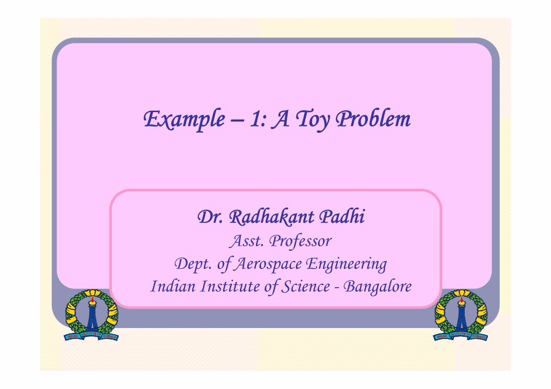
ExampleBoundary Conditions
Define
Solution
( )( )
( )( )
( )( )
1 1 1
2 2 2
0 2 2 50,
0 2 2 20x xx x
λλ
−⎡ ⎤ ⎡ ⎤ ⎡ ⎤⎡ ⎤= =⎢ ⎥ ⎢ ⎥ ⎢ ⎥⎢ ⎥ −⎣ ⎦⎣ ⎦ ⎣ ⎦ ⎣ ⎦
[ ]1 2 1 2TZ x x λ λ
Z AZ=
0 1 0 00 1 0 10 0 0 00 0 1 1
A
⎡ ⎤⎢ ⎥− −⎢ ⎥=⎢ ⎥⎢ ⎥−⎣ ⎦
( ) AtZ t e C=
ADVANCED CONTROL SYSTEM DESIGN Dr. Radhakant Padhi, AE Dept., IISc-Bangalore
21
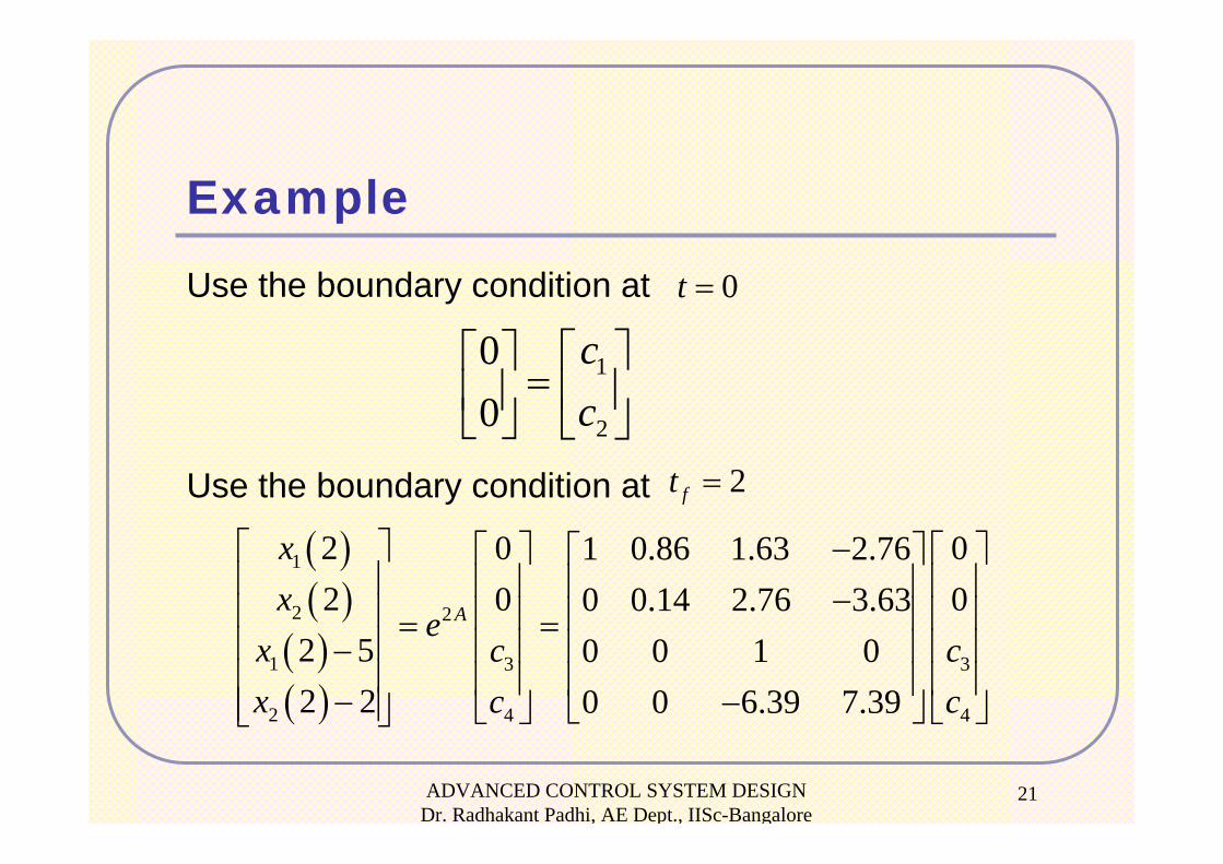
ExampleUse the boundary condition at
Use the boundary condition at
0t =
1
2
00
cc⎡ ⎤⎡ ⎤
= ⎢ ⎥⎢ ⎥⎣ ⎦ ⎣ ⎦
2ft =
( )( )
( )( )
1
2 2
1 3 3
2 4 4
2 0 01 0.86 1.63 2.762 0 00 0.14 2.76 3.63
2 5 0 0 1 02 2 0 0 6.39 7.39
A
xx
ex c cx c c
⎡ ⎤ −⎡ ⎤ ⎡ ⎤⎡ ⎤⎢ ⎥ ⎢ ⎥ ⎢ ⎥⎢ ⎥−⎢ ⎥ ⎢ ⎥ ⎢ ⎥⎢ ⎥= =⎢ ⎥ ⎢ ⎥ ⎢ ⎥⎢ ⎥−⎢ ⎥ ⎢ ⎥ ⎢ ⎥⎢ ⎥− −⎢ ⎥ ⎣ ⎦⎣ ⎦ ⎣ ⎦⎣ ⎦

ADVANCED CONTROL SYSTEM DESIGN Dr. Radhakant Padhi, AE Dept., IISc-Bangalore
22
ExampleFour equations and four unknowns:
( )( )
1
2
3
4
1 0 1.63 2.76 020 1 2.76 3.63 021 0 1 0 50 1 6.39 7.39 2
xx
cc
− ⎡ ⎤⎡ ⎤ ⎡ ⎤⎢ ⎥⎢ ⎥ ⎢ ⎥− ⎢ ⎥⎢ ⎥ ⎢ ⎥=⎢ ⎥⎢ ⎥ ⎢ ⎥−⎢ ⎥⎢ ⎥ ⎢ ⎥−⎣ ⎦ ⎣ ⎦⎣ ⎦
( )( )
11
2
3
4
1 0 1.63 2.76 0 2.3020 1 2.76 3.63 0 1.3321 0 1 0 5 2.700 1 6.39 7.39 2 2.42
xx
cc
−−⎡ ⎤ ⎡ ⎤ ⎡ ⎤ ⎡ ⎤⎢ ⎥ ⎢ ⎥ ⎢ ⎥ ⎢ ⎥−⎢ ⎥ ⎢ ⎥ ⎢ ⎥ ⎢ ⎥= =⎢ ⎥ ⎢ ⎥ ⎢ ⎥ ⎢ ⎥− −⎢ ⎥ ⎢ ⎥ ⎢ ⎥ ⎢ ⎥− −⎣ ⎦ ⎣ ⎦ ⎣ ⎦⎣ ⎦
ADVANCED CONTROL SYSTEM DESIGN Dr. Radhakant Padhi, AE Dept., IISc-Bangalore
23
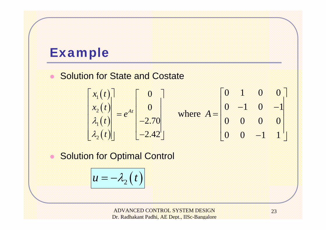
ExampleSolution for State and Costate
Solution for Optimal Control
( )( )( )( )
1
2
1
2
00
2.702.42
At
x tx t
ett
λλ
⎡ ⎤ ⎡ ⎤⎢ ⎥ ⎢ ⎥⎢ ⎥ ⎢ ⎥=⎢ ⎥ ⎢ ⎥−⎢ ⎥ ⎢ ⎥−⎢ ⎥ ⎣ ⎦⎣ ⎦
0 1 0 00 1 0 1
where 0 0 0 00 0 1 1
A
⎡ ⎤⎢ ⎥− −⎢ ⎥=⎢ ⎥⎢ ⎥−⎣ ⎦
( )2u tλ= −

Example – 2: Double Integrator Problem(Relevance: Satellite Attitude Control Problem)
Dr. Radhakant PadhiAsst. Professor
Dept. of Aerospace EngineeringIndian Institute of Science - Bangalore
x u=

ADVANCED CONTROL SYSTEM DESIGN Dr. Radhakant Padhi, AE Dept., IISc-Bangalore
25
Double Integrator Problem2u x= 2 1x x= 1x y=
∫ ∫
( ) [ ]T
2 2
0
Consider a double integrator problem as shown in the above figure.
Find such ( ) that the system initial values 0 = 10 0 aredriven to the origin by minimizing
12
(1) : unspecified
(2
ft
f
f
u t X
J t u dt
t
= + ∫Note :
) Control variable ( ) is unconstrainedu t

ADVANCED CONTROL SYSTEM DESIGN Dr. Radhakant Padhi, AE Dept., IISc-Bangalore
26
Double Integrator Problem
[ ]
( ) ( )
1 1
2 2
1
2
System dynamics
0 1 00 0 1
1 0 (not required)
Boundary Condition
10 00 ,
0 0
BXA
C
f
x xU AX BU
x x
xy CX
x
X X t
⎡ ⎤ ⎡ ⎤⎡ ⎤ ⎡ ⎤= + = +⎢ ⎥ ⎢ ⎥⎢ ⎥ ⎢ ⎥⎣ ⎦ ⎣ ⎦⎣ ⎦ ⎣ ⎦
⎡ ⎤= =⎢ ⎥
⎣ ⎦
⎡ ⎤ ⎡ ⎤= =⎢ ⎥ ⎢ ⎥⎣ ⎦ ⎣ ⎦
Solution :

ADVANCED CONTROL SYSTEM DESIGN Dr. Radhakant Padhi, AE Dept., IISc-Bangalore
27
Double Integrator Problem
[ ]
Controllability Matrix
0 0 1 0 0 11 0 0 1 1 0
1 0
Hence, the system is controllable.
M B AB
M
⎡ ⎤⎡ ⎤ ⎡ ⎤ ⎡ ⎤ ⎡ ⎤= = =⎢ ⎥⎢ ⎥ ⎢ ⎥ ⎢ ⎥ ⎢ ⎥
⎣ ⎦ ⎣ ⎦ ⎣ ⎦ ⎣ ⎦⎣ ⎦= − ≠
Controllability Check :

ADVANCED CONTROL SYSTEM DESIGN Dr. Radhakant Padhi, AE Dept., IISc-Bangalore
28
Necessary Conditions of Optimality
( )2
2
12
(1) State Eq: H(2) Optimal Control Eq: 0
0
(3) Costate Eq:
T
T
T
T
H u AX Bu
X AX Bu
uu Bu B
H AX
λ
λ
λ λ
λ λ
= + +
= +∂
=∂+ =
= − = −∂
= − = −∂

ADVANCED CONTROL SYSTEM DESIGN Dr. Radhakant Padhi, AE Dept., IISc-Bangalore
29
Optimal Control Solution
11
2 12
1 1 1
2 1 1
2 1 2
2 1 2
00 01 0
0
TA
c
cc t c
u c t c
λλλ
λ λλ
λ λ
λ λλ
λ
⎡ ⎤ ⎡ ⎤ ⎡ ⎤⎡ ⎤= − = − =⎢ ⎥ ⎢ ⎥ ⎢ ⎥⎢ ⎥ −⎣ ⎦ ⎣ ⎦ ⎣ ⎦⎣ ⎦
= ⇒ =
= − = −= − +
∴ = − = −

ADVANCED CONTROL SYSTEM DESIGN Dr. Radhakant Padhi, AE Dept., IISc-Bangalore
30
Optimal State Solution
1 22
2 1 2
2
2 1 2 3
3 2
1 2 1 2 3 4
However,
Hence
2
6 2
x xxx c t cu
tx c c t c
t tx x dt c c c t c
⎡ ⎤ ⎡ ⎤⎡ ⎤= =⎢ ⎥ ⎢ ⎥⎢ ⎥ −⎣ ⎦⎣ ⎦ ⎣ ⎦
= − +
= = − + +∫

ADVANCED CONTROL SYSTEM DESIGN Dr. Radhakant Padhi, AE Dept., IISc-Bangalore
31
Optimal State Solution
( )( )
( )( )
( )( )
1 4
2 3
3 21 2
1
22 12
3 21 21
2122
Using the B.C. at 0 :
0 100 0
106 2
2Using the B.C at :
10 06 20
2
f
f ff
ff f
t
x cx c
c ct tx tx t c t c t
t t
c ct tx t
cx t t c t
=
⎡ ⎤ ⎡ ⎤ ⎡ ⎤= =⎢ ⎥ ⎢ ⎥ ⎢ ⎥
⎣ ⎦⎣ ⎦⎣ ⎦⎡ ⎤− +⎢ ⎥⎡ ⎤
∴ = ⎢ ⎥⎢ ⎥⎢ ⎥⎣ ⎦ −⎢ ⎥⎣ ⎦
=
⎡ ⎤− +⎡ ⎤ ⎢ ⎥ ⎡ ⎤⎢ ⎥ = =⎢ ⎥ ⎢ ⎥⎢ ⎥ ⎣ ⎦⎢ ⎥−⎣ ⎦ ⎢ ⎥⎣ ⎦

ADVANCED CONTROL SYSTEM DESIGN Dr. Radhakant Padhi, AE Dept., IISc-Bangalore
32
Transversality Conditions (tf : free)
( )
[ ]
( ) ( ) ( ) ( )
( )
2
22
1 2
221 2
1 2 1 2
2
1 2
2 2 21 1 2 2
22
2
2
12
4 2
ff
f
f
tt
Tf
t
t
ff f f
f
f f f
Ht
ut AX Bu
xuu
c t ct x t c t c
c t c
t c t c c t c
ϕ
λ
λ λ
λ
∂= −
∂
⎡ ⎤= − + +⎢ ⎥
⎣ ⎦
⎡ ⎤⎡ ⎤= − +⎢ ⎥⎢ ⎥
⎣ ⎦⎣ ⎦
⎡ ⎤−⎢ ⎥= − + − −⎢ ⎥⎣ ⎦
= −
= − +
0 (B.C.)

ADVANCED CONTROL SYSTEM DESIGN Dr. Radhakant Padhi, AE Dept., IISc-Bangalore
33
Transversality Conditions (tf : free)
( )
1 2
3 21 2
21 2
2 2 21 1 2 2
1 2
In summary, we have to solve for , and from:
3 60 0
2 0
2 4 0
At this point, one can solve , from first twoequations in terms of and subtitute them in
f
f f
f f
f f
f
c c t
c t c t
c t c t
c t c c t c
c ct
− + =
− =
− + + =
the
third equation. Then the resulting nonlinear equationin can be solved (preferably in closed form). However, one must
discard unrealistic solutions (e.g. 0 is unrealistic).
One may use nu
f
f
t
t ≤
Note : merical tehniques (like Newton-Raphson technique)

ADVANCED CONTROL SYSTEM DESIGN Dr. Radhakant Padhi, AE Dept., IISc-Bangalore
34
Transversality Conditions (tf : free)
( ) [ ]
( ) [ ]
1
22
2
1 22
T
T
2.025Finally, 3.95
/ 4
Hence, the optimal solution is given by:2.025 3.95
3.95and it will take 3.901 time units to reach = 0 0 ,
4starting from 0 = 10 0Note: (1)
f
f f
cct c
u c t c t
t X
X
⎡ ⎤ ⎡ ⎤⎢ ⎥ ⎢ ⎥=⎢ ⎥ ⎢ ⎥⎢ ⎥ ⎢ ⎥⎣ ⎦⎣ ⎦
= − = −
= =
It is an open-loop control law (2) The application of control has to be terminated at ft

ADVANCED CONTROL SYSTEM DESIGN Dr. Radhakant Padhi, AE Dept., IISc-Bangalore
35
References on Optimal Control Design
T. F. Elbert, Estimation and Control Systems, Von Nostard Reinhold, 1984. A. E. Bryson and Y-C Ho, Applied Optimal Control, Taylor and Francis, 1975.R. F. Stengel, Optimal Control and Estimation, Dover Publications, 1994.D. S. Naidu, Optimal Control Systems, CRC Press, 2002.A. P. Sage and C. C. White III, Optimum Systems Control (2nd Ed.), Prentice Hall, 1977.D. E. Kirk, Optimal Control Theory: An Introduction, Prentice Hall, 1970.

ADVANCED CONTROL SYSTEM DESIGN Dr. Radhakant Padhi, AE Dept., IISc-Bangalore
36