Optimal Capital Structure and Industry Dynamicspeople.bu.edu/miaoj/IndustryJF.pdf · THE JOURNAL OF FINANCE • VOL. LX, NO. 6 • DECEMBER 2005 Optimal Capital Structure and Industry

THE JOURNAL OF FINANCE • VOL. LX, NO. 6 • DECEMBER 2005

Optimal Capital Structureand Industry Dynamics

JIANJUN MIAO∗

ABSTRACT

This paper provides a competitive equilibrium model of capital structure and industrydynamics. In the model, firms make financing, investment, entry, and exit decisionssubject to idiosyncratic technology shocks. The capital structure choice reflects thetradeoff between the tax benefits of debt and the associated bankruptcy and agencycosts. The interaction between financing and production decisions influences the sta-tionary distribution of firms and their survival probabilities. The analysis demon-strates that the equilibrium output price has an important feedback effect. This effecthas a number of testable implications. For example, high growth industries have rel-atively lower leverage and turnover rates.

THE INTERACTION BETWEEN CAPITAL STRUCTURE and product market decisions hasrecently received considerable attention in both economics and finance. Begin-ning with Brander and Lewis (1986, 1988) and Maksimovic (1988), a growingnumber of theoretical papers investigate this interaction. In addition, many em-pirical studies (Chevalier (1995a, 1995b), Phillips (1995), Kovenock and Phillips(1997), Maksimovic and Phillips (1998), Zingales (1998), Lang, Ofek, and Stulz(1996), Mackay and Phillips (2004)) examine the relation between capital struc-ture and firm entry, exit, investment and output decisions.1 These studies gen-erally document the following:

(1) Industry output is negatively associated with the average industry debtratio.

(2) Plant closings are positively associated with debt and negatively associ-ated with plant-level productivity.

(3) Firm entry is positively associated with debt of incumbents.(4) Firm investment is negatively associated with debt.(5) There is substantial inter- and intra-industry variation in leverage.

∗Jianjun Miao is at the Department of Economics, Boston University. I thank Larry Epsteinand Erwan Morellec for constant support and advice. I also thank seminar participants at manyinstitutions, especially, Rui Albuquerque, Mike Barclay, Dan Bernhardt, Pierre Collin-Dufresne,Chris Hennessy, Ludger Hentschel, Burton Hollifield, Hugo Hopenhayn, Boyan Jovanovic, LarryKotlikoff, Hayne Leland, John Long, Hanno Lustig, Josef Perktold, Victor Rios-Rull, Marc Rysman,Jacob Sagi, Nancy Stokey, Sheridan Titman, and Neng Wang for helpful comments. I am alsograteful to an anonymous referee and the editor Robert Stambaugh for extremely helpful commentsand suggestions.

1 Early studies that relate the cross-sectional behavior of leverage to industry characteristicsinclude Bradley, Jarrell, and Kim (1984) and Titman and Wessels (1988), among others.

2621

2622 The Journal of Finance

It is well known that debt causes the underinvestment and asset substitutionproblems identified by Myers (1977) and Jensen and Meckling (1976). How-ever, it is important to emphasize that simply taking leverage as an exogenousregressor may be misleading. This is because rational firms may anticipatethe effect of leverage on product/input market behavior so that the latter mayinfluence capital structure choices. This endogeneity problem makes the in-terpretation of the above empirical evidence controversial. As pointed out byZingales (1998, p. 905), “in the absence of a structural model we cannot deter-mine whether it is the product market competition that affects capital structurechoices or a firm’s capital structure that affects its competitive position and itssurvival.”

The main contribution of my paper is to fill this theoretical gap by pro-viding an industry equilibrium model in which capital structure choices andproduction decisions are simultaneously influenced by the same exogenousfactors. The second contribution of my paper is related to industrial organi-zation. Many empirical studies in industrial organization have documentedcross-industry differences in firm turnover. However, little theoretical re-search has been devoted to understanding the impact of financing policieson firm turnover.2 The present paper adds to this literature both by show-ing how the interaction between financing and production decisions influ-ences firm turnover and by providing new testable predictions regarding itsdeterminants.

The basic structure of the model is as follows. The model features a con-tinuum of firms facing idiosyncratic technology shocks. These firms are con-trolled by shareholders and make financing, entry, exit, and production deci-sions. The capital structure choice is modeled by incorporating approaches ofModigliani and Miller (1958, 1963), Kraus and Litzenberger (1973), and Jensenand Meckling (1976).3 Moreover, this choice reflects the equilibrium interac-tion between financing and production/investment decisions. Specifically, pro-duction/investment decisions are chosen to maximize equity value after debtis in place so that shareholder–bondholder conflicts lead to agency costs asin Jensen and Meckling (1976) and Myers (1977).4 The initial capital struc-ture choice, made ex ante, trades off the tax benefits of debt versus the associ-ated bankruptcy and agency costs. Thus, the model departs from the standardModigliani–Miller framework.

In a long-run stationary industry equilibrium, there is a stationary distri-bution of surviving firms. These firms exhibit a wide variation of leverage.

2 See Caves (1998) for a survey of the empirical literature on firm turnover. See Jovanovic (1982),Hopenhayn (1992a, 1992b), and Ericson and Pakes (1995) for important theoretical models ofindustry dynamics. All these papers assume that firms are all-equity financed.

3 See Harris and Raviv (1991) for a survey of the theory of capital structure. They point out that“with regard to further theoretical work, it appears that models relating to products and inputs areunderexplored, while the asymmetric information approach has reached the point of diminishingreturns.” (pp. 299–300)

4 I do not consider conflicts between shareholders and managers. Morellec (2004) examines theseconflicts in a contingent claims framework.

Optimal Capital Structure and Industry Dynamics 2623

Furthermore, all industry-wide equilibrium variables are constant over time,although individual firms are continually adjusting, with some of them expand-ing, others contracting, some starting up, and others closing down.

I derive a closed-form solution for the unique stationary equilibrium so thatthe model can be analyzed tractably. I also study the effects on the equilibriumof changes in growth of technology, riskiness of technology, starting distributionof technology, fixed operating cost, entry cost, bankruptcy cost, and corporatetax.

I now highlight the main mechanism operating in the model by an example.Consider the effect of an increase in technology growth in a risk-neutral envi-ronment. First, this increase has a cash flow effect, in the sense that operatingprofits are higher. It also has an option effect in the sense that it changes theexpected appreciation in the value of the option to default. These two effectsraise firm value and the benefit of remaining active. Thus, the firm is less likelyto default, and has lower expected bankruptcy costs. The standard single-firmtradeoff theory then predicts that the firm should issue more debt. However,the prediction that high growth firms have high leverage is refuted by manyempirical studies (see Rajan and Zingales (1995), Barclay, Morellec, and Smith(2002), and references cited therein).

In the present industry equilibrium model, there is an important pricefeedback effect associated with an increase in technology growth. That is,potential entrants will anticipate increased firm value and hence prefer toenter the industry. As a result, product market competition causes the out-put price to fall. The decreased output price influences the firm’s financingand liquidation/exit decisions. In particular, in contrast to standard single-firm tradeoff models, this feedback effect may dominate so as to raise exitprobabilities, lower coupon payments, and lower the average industry leverageratio.

The model also has important implications for industry dynamics. Specifi-cally, an increase in the rate of technology growth and the induced increase inthe exit threshold have a selection effect in that the stationary distribution ofsurviving firms changes. This selection effect causes inefficient firms to exitand be replaced by new entrants, thereby leading to higher industry outputand a lower turnover rate.

The present paper relates to three strands of literature. One strand begin-ning with Black and Scholes (1973) and Merton (1974) is in the framework ofdynamic contingent claims analysis. Brennan and Schwartz (1984), Mello andParsons (1992), Mauer and Triantis (1994), and Titman and Tsyplakov (2002)analyze the interaction between investment and financing decisions using nu-merical methods. Dixit (1989) studies entry and exit decisions under all-equityfinancing. Leland (1994, 1998), Leland and Toft (1996), Goldstein, Ju, and Le-land (2001), and Morellec (2001) analyze corporate asset valuation and optimalcapital structure using analytical methods. All these models consider a single-firm environment. Under perfect competition, Leahy (1993) analyzes entry andexit under all equity financing in an industry equilibrium framework. Fries,Miller, and Perraudin (1997) generalize Leahy’s model and study how entry


and exit affect corporate asset valuation and capital structure.5 Lambrecht(2001) analyzes the impact of debt financing on entry and exit in an oligopolyenvironment.

Another strand is based on the framework developed by Hopenhayn (1992a,1992b) and Hopenhayn and Rogerson (1993), where the concept of stationaryequilibrium is introduced to analyze industry dynamics. Dixit and Pindyck(1994, Chapter 8) study industry investment in a similar framework. They as-sume firms exit the industry exogenously through sudden deaths. Most papersin this strand assume that firms are all-equity financed. Cooley and Quadrini(2001) introduce capital structure decisions into this framework and studyhow financial frictions account for the negative dependence of firm dynam-ics (growth, job reallocation, and exit) on size and age. They assume exoge-nous exit and consider standard one-period debt contracts based on asymmetricinformation.

The third strand of literature is based on strategic models. Some papers inthis strand (Brander and Lewis (1986, 1988) and Maksimovic (1988)) arguethat product market competition becomes “tougher” when leverage increases,while others (e.g., Poitevin (1989), Bolton and Scharfstein (1990), Dasguptaand Titman (1998)) reach the opposite conclusion. Since most models in thisstrand are essentially static, it seems that they are not suitable to address thequestions of industry dynamics and corporate asset valuation.

My model combines elements of the first two strands of literature. In particu-lar, I incorporate capital structure decisions into the framework of Hopenhayn(1992a), using the contingent claims analysis. This allows me to derive anumber of new predictions regarding the relation between leverage and firmturnover. My model is also closely related to Fries et al. (1997) and Lambrecht(2001). Unlike Lambrecht (2001), I study perfectly competitive industries. Inaddition, unlike these two papers, where uncertainty comes from aggregate in-dustry demand shocks, I assume that firms face idiosyncratic technology shocksas in Hopenhayn (1992a). The basic intuition behind the difference betweenfirm-specific shocks and industry-wide shocks is explained in Dixit and Pindyck(1994, Chapter 8).

The remainder of the paper is organized as follows. Section I sets up themodel. Section II studies a single firm’s optimal capital structure choice in anindustry setting. Section III derives closed-form solutions for the unique equi-librium. Section IV analyzes properties of the equilibrium. Section V concludes.Technical details are relegated to appendices.

I. The Model

Consider an industry consisting of a large number of firms. Suppose infor-mation is perfect and all investors are risk neutral and discount future cash

5 Maksimovic and Zechner (1991) present a three-period industry equilibrium model in whichfirms can adopt different technologies. They do not study entry and exit decisions. See Williams(1995) for an extension in a four-period model.


flows at a constant risk-free rate r > 0. The assumption of risk neutrality doesnot lose any generality. If agents are risk averse, the analysis may be conductedunder the risk-neutral measure (see Harrison and Kreps (1979)).

Time is continuous and varies over [0, ∞). Uncertainty is represented bya probability space (�, F , P) over which all stochastic processes are defined.The objective is to study long-run stationary industry equilibria in which allindustry-wide aggregate variables are constant (see Section I.D for a formaldefinition). In particular, the equilibrium output price is constant, and there isan equilibrium stationary distribution of surviving firms.

A. Industry Demand

Industry demand is given by a decreasing function. For simplicity, take thefollowing iso-elastic functional form:

p = Y − 1ε , (1)

where p is the output price, Y is the industry output, and ε > 0 is the priceelasticity of demand.

B. Firms

There is a continuum of firms. Firms behave competitively, taking prices ofoutput and input as given. At each date, each firm suffers independently exoge-nous death under the Poisson process with parameter η > 0. This assumptioncaptures the fact that some firms exit the industry for reasons that are notrelated to bankruptcy. In addition, it is important to ensure the existence of astationary distribution of firms, since the technology shock is a nonstationaryprocess, as I describe next.

B.1. Technology

Each firm rents capital at the rental rate R to produce output with the produc-tion function F : R+ → R+, F (k) = kν , where ν ∈ (0, 1). The decreasing-returns-to-scale assumption ensures that the firm’s profit is positive so that the decisionproblem of entry and exit studied below is meaningful. Capital depreciates con-tinuously at a constant rate δ > 0. Thus, the rental rate R is equal to r + δ.

Firms are ex ante identical in that their technology or productivity shocksare drawn from the same distribution. They differ ex post in the realization ofidiosyncratic shocks. Suppose that there is no aggregate uncertainty, and a lawof large numbers for a continuum of random variables is such that industryaggregates are constant (see Judd (1985), Feldman and Gilles (1985), and Miao(2004) for discussion in the discrete time case).

For an individual firm, the technology shock process (zt)t≥0 is governed by ageometric Brownian motion


dzt/zt = µz dt + σz dW t , (2)

where µz and σz are positive constants. Here (Wt)t≥0 is a standard Brownianmotion representing firm-specific uncertainty.

B.2. Profit Function

At each time, each firm incurs a fixed operating cost cf > 0 to produce output.Corporate income is taxed at the rate τ with full loss-offset provisions.6 Definethe after-tax profit function � as

�(z; p) = maxk≥0

(1 − τ )(pz F (k) − δk − c f ) − rk. (3)

Note that according to the U.S. tax system, the depreciation of capital is tax-deductible, but the interest cost of capital is not. Profit maximization impliesthe following neoclassical investment rule:

pz F ′(k) = r/(1 − τ ) + δ. (4)

That is, the marginal product of capital is equal to the tax-adjusted user cost ofcapital. Using this equation, one can solve for the capital demand and outputsupply

k(z; p) = zγ

(pν

r/(1 − τ ) + δ

)γ

,

y(z; p) = z F (k(z; p)) = zγ

(pν

r/(1 − τ ) + δ

)νγ

, (5)

where I define

γ ≡ 11 − ν

. (6)

Substituting the above equations into (3) yields the after-tax profit function

�(z; p) = (1 − τ )[a(p)zγ − c f

], (7)

where

a(p) ≡ pγ (1 − ν)(

ν

r/(1 − τ ) + δ

)νγ

. (8)

It is convenient to define the before-tax profit function

π (z; p) ≡ a(p)zγ − c f . (9)

This function will be used repeatedly below.

6 I abstract from personal taxes in the paper.


B.3. Debt Contracts

Because interest payments to debt are tax deductible, each firm has an in-centive to issue debt. In order to stay in a time-homogenous environment, Iconsider debt contracts with infinite maturity, as in Leland (1994) and Duffieand Lando (2001). Debt is issued at par. The debt contract specifies a perpet-ual flow of coupon payments b to bondholders. The remaining cash flows fromoperation accrue to shareholders. If the firm defaults on its debt obligations, itis immediately liquidated. Upon default, bondholders get the liquidation valueand shareholders get nothing.

B.4. Liquidation Value

Suppose that debt reorganization is so costly that after default the firm isimmediately liquidated and exits the industry.7 I model liquidation value as afraction α ∈ (0, 1) of the unlevered firm value A(z; p). The remaining fractionaccounts for bankruptcy costs. One can model liquidation value as a generalfunction of the output price X(p) as in Fries et al. (1997). Here, I follow Melloand Parsons (1992). Unlevered firm value is equal to the after-tax present valueof profits, plus the option value associated with abandonment opportunities.Normalize the abandonment value of the firm to zero. The firm then choosesan abandonment time T so that unlevered firm value can be formally describedas

A(z; p) = (1 − τ ) supT∈T

Ez[∫ T

0e−(r+η)tπ (zt ; p) dt

], (10)

where the maximization is over the set T of all stopping times relative to thefiltration generated by the Brownian motion (Wt)t≥0, Ez is the expectation op-erator for the process (zt)t≥0 starting at z, and the factor e−ηt accounts for thepossibility of Poisson deaths.

B.5. Investment and Liquidation Decisions

At each date t, after servicing coupon payments b, residual cash flows(1 − τ )(pztF(kt) − δkt − cf − b) − rkt are distributed to shareholders as divi-dends. Shareholders select the investment and default policy to maximize thevalue of their claims, taking price p as given. Assume that default is triggeredby the decision of shareholders to cease raising additional equity to meet thecoupon payment, as in Mello and Parsons (1992), Leland (1994), Fries et al.(1997), Lambrecht (2001), and Duffie and Lando (2001).

The following problem describes the investment and liquidation decisionsmade by a typical firm with the current level of technology shock z and couponpayment b:

7 This assumption could be relaxed by allowing debt to be reorganized through, for example, debtexchange offers as in Mella-Barral (1995) and Lambrecht (2001). This kind of analysis is, however,beyond the scope of this paper.


e(z, b; p)

= sup(kt )t≥0,T∈T

Ez{∫ T

0e−(r+η)t [

(1 − τ )(pzt F (kt) − δkt − c f − b

) − rkt]

dt}

.

(11)

Using the previously defined before-tax profit function, one can rewrite thisproblem as

e(z, b; p) = supT∈T

(1 − τ ) Ez[∫ T

0e−(r+η)t(π (zt ; p) − b) dt

], (12)

where π (zt; p) is given in (9). The expression e(z, b; p) represents the equity valueof the firm. Since one can show that it is increasing in z, the default decision isdescribed by a trigger policy whereby the firm is immediately liquidated andexits the industry once its technology shock (zt)t≥0 falls below an endogenouslydetermined threshold zd(b; p) (see Duffie and Lando (2001)). In what follows,without risk of confusion, I may simply use zd to denote zd(b; p).

The equity-value-maximizing investment policy is similar to that describedby the neoclassical rule (4). The difference is that here, investment takes placeonly in the no-default region z > zd(b; p). This is related to the underinvestmentproblem of debt pointed out by Myers (1977) and is consistent with the empiricalevidence mentioned in the introduction.

Notice that the limited liability feature of equity is embodied in problem (11)since equity value is always positive before default (z > zd(b; p)), and is zeroonly upon default (z = zd(b; p)).

B.6. Debt Value and Firm Value

The arbitrage-free value of debt is equal to the sum of the present value ofcoupon payments accruing to bondholders until the default time and the presentvalue of liquidation value upon default. That is, debt value d(z, b; p) is given by

d (z, b; p) = Ez[∫ Tzd

0e−(r+η)t bdt

]+ αA(zd ; p)Ez[e−(r+η)Tzd

], (13)

where Ty denotes the first time that the process (zt)t≥0 falls to some boundaryvalue y > 0. Firm value v(z, b; p) is the sum of equity value and debt value,

v(z, b; p) = e(z, b; p) + d (z, b; p). (14)

B.7. Entry and Financing

At each date there is a continuum of potential entrants. Upon entry firmsincur a fixed sunk cost ce. This cost can be financed by equity and debt. Afterentry, a firm’s initial level of technology z is drawn from the distribution ζ , which


is uniform over [z¯, z̄]. This firm is then in the same position as an incumbent

with the initial level of technology z. However, firms differ over time becausethey may experience different idiosyncratic shocks. Note that the uniform entrydistribution is important to derive a closed-form solution for the stationarydistribution of incumbents.

Assume that z¯

> zd (b; p). Since zd is endogenous, this assumption must beverified in equilibrium. I rule out the case in which the initial draw of the tech-nology shock is below the default threshold so that the entrant is immediatelyliquidated and exits the industry.

Before entry, firms are identical and they do not know their initial technologylevels and subsequent random evolution of technology. In a competitive equi-librium, if there is positive entry, then the expected benefit of entry must beequal to the entry cost. That is, the following entry condition must hold,∫ z̄

z¯

v(z, b; p)ζ (dz) = ce. (15)

Finally, upon entry firms may adjust the capital structure in order to balancethe benefit and cost of debt. The optimal coupon rate b∗(p) is chosen to maximizethe expected value of the firm,

∫ z̄z¯

v(z, b; p)ζ (dz). Since all firms are ex anteidentical, they choose the same optimal coupon rate. For tractability, I assumethat firms do not readjust debt after entry, as in most contingent claims modelsof capital structure.

B.8. Timeline for Decisions

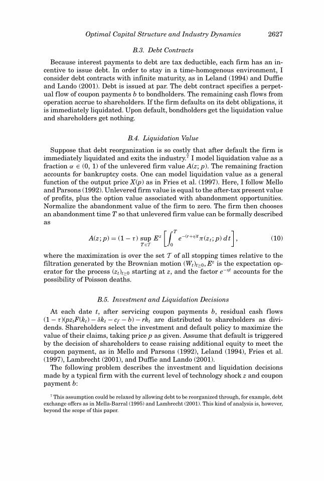
In summary, the sequence of events and the timing of decisions for a typicalfirm are described in Figure 1.

C. Aggregation

In a long-run steady state, there is a stationary distribution of survivingfirms µ and a constant entry rate N.8 Note that the distribution µ is not aprobability measure. For any Borel set B in the real line, µ(B) describes thenumber of surviving firms whose technology shocks lie in the set B. Since afirm exits when its technology shock falls below zd(b; p), the support of µ is theinterval [zd(b; p), ∞). Using this stationary distribution, aggregate variablescan be computed; for example, industry output supply is given by

Y (µ, b; p) =∫ ∞

zd (b;p)y(z; p)µ(dz), (16)

8 The entry (exit) rate is defined as the number of firms entering (going bankrupt and exiting)the industry at each time. The same term used in some empirical studies (e.g., Dunne et al. (1988))corresponds to the turnover rate defined later.


�z0

�

Drawn from auniform distribution

�

Entryfinancing

zt

�

Follows a geometricBrownian motion

�Exit, Poisson deathdefault, liquidation

Stay inproduction

Figure 1. Timeline for decisions.

where y(z; p) is given in (5). Intuitively, suppose z takes finitely many valueszi ∈ [zd (b; p), ∞), i = 1, . . . , n, and µ(zi) is the mass of surviving firms whosetechnology level is zi. Then industry output supply is given by

Y (µ, b; p) =n∑

i=1

y(zi; p)µ(zi). (17)

D. Equilibrium

A stationary industry equilibrium with exogenous leverage, (p∗, ze, N∗, µ∗),consists of a constant output price p∗, an exit threshold ze = zd(b; p∗), an entryrate N∗, and a distribution of incumbents µ∗ such that (i) firms solve problem(11); (ii) the market clears

p∗ = Y (µ∗, b; p∗)−1/ε, (18)

where Y(·) is given in (16); (iii) the entry condition (15) holds; and, (iv) thedistribution µ∗ is an invariant measure over [ze, ∞).

In this equilibrium, the coupon rate b is exogenously given. When b is cho-sen to maximize firm value, the resulting equilibrium is called the station-ary equilibrium with endogenous leverage. Such an equilibrium is denoted by(po, zo

e , No, µo).Conditions (i)–(iii) in the above definition are standard requirements for a

competitive equilibrium. Condition (iv) requires that, in a long-run steady state,the distribution of firms be constant over time. This is possible because there isa continuum of firms that are subject to idiosyncratic shocks and a law of largenumbers is assumed. As pointed out by Dixit and Pindyck (1994, p. 277), “at theindustry level, the shocks and responses of firms can aggregate into long-runstationary conditions, so that the industry output and price are nonrandom.However, the equilibrium level of these variables is affected by the parametersof firm-specific uncertainty. Also, behind the aggregate certainty lies a greatdeal of randomness and fluctuations: firms enter, invest, and exit in responseto the shocks to their individual fortunes.”


To better understand condition (iv), it is helpful to use a discrete time approx-imation similar to that in Hopenhayn (1992a). The following equation describesthe evolution of firm distributions:

µt+dt(B) = (1 − η dt

) ∫ ∞

ze

Q(B | z)µt(dz) + N ∗ζ ([z¯, z̄] ∩ B) dt. (19)

The interpretation is as follows: At any date t, let µt be the distribution of firmsat date t. After an instant dt, firms transit to the set B at date t + dt according tothe transition function Q(B | z). Each firm survives with probability (1 − η dt).Moreover, each firm exits the industry when its technology shocks fall belowze. Thus, the first term in (19) describes the mass of firms that lie in the setB at date t + dt. The second term in (19) describes the mass of new entrantsentering the set B. The sum of these two terms is equal to the total mass offirms that lie in the set B at date t + dt, which is µt+dt(B). In the long-runstationary equilibrium, this mass must not change over time. This determinesthe invariant distribution µ∗(B). Note that firms are identified by the technologylevels z. The mass of firms with technology levels lying in B is constant overtime. However, the actual identities of firms occupying these positions may keepchanging.

II. Optimal Capital Structure

In this section, I fix the output price p and consider a single firm’s capitalstructure decision. This decision is modeled in the spirit of the standard EBIT-based single-firm contingent claims models, such as Mello and Parsons (1992)and Goldstein et al. (2001). However, different from these models, investmentpolicies are not fixed, and the product market influences the capital structuredecision through the output price.

A. Unlevered Firm Value

I begin by deriving unlevered firm value. Because unlevered firm value isincreasing in z, the solution to (10) is described by a threshold value zA. Thefirm is abandoned the first time the technology shock falls below zA. To solvefor this threshold value zA and unlevered firm value, let

A(z; p | y) = (1 − τ )Ez[∫ Ty


](20)

be unlevered firm value given any threshold level y > 0. Here Ty denotes thefirst passage time of the process (zt)t≥0 starting from z to y. The abandonmentthreshold zA is determined by the smooth-pasting condition

∂ A(z; p | z A)∂z

∣∣∣∣z=z A

= 0. (21)

The following proposition describes unlevered firm value and the abandonmentdecision.


PROPOSITION 1: Suppose

λ ≡ r + η − µzγ − σ 2z γ (γ − 1)/2 > 0. (22)

Then unlevered firm value is given by

A(z; p) = (1 − τ )�(z; p) − (1 − τ )�(z A; p)(

zz A

)ϑ

, z ≥ z A, (23)

where

ϑ ≡ 1σ 2

z

[(σ 2

z

/2 − µz

) −√

2(r + η)σ 2z + (

σ 2z

/2 − µz

)2]

< 0, (24)

�(z; p) ≡ Ez[∫ ∞


]= a(p)

λzγ − c f

r + η, (25)

and

z A(p) =[

ϑλc f

(ϑ − γ )(r + η)a(p)

]1/γ

. (26)

The firm is abandoned the first time its technology process falls below the thresh-old value zA.

Note that � (z; p) in (25) represents the before-tax present value of the profitflow. Assumption (22) ensures that � (z; p) is finite. Equation (23) implies thatunlevered firm value is equal to the present value of after-tax profits plus theoption value of abandonment. Since �(z A, p) = γ

ϑ − γ

c f

r + η< 0, the firm is not

abandoned as soon as losses are incurred: Only if the firm’s technology shock isbad enough, is the firm abandoned—because abandonment is irreversible andwaiting has positive option value.

B. Liquidation Decision and Levered Equity Value

Recall that the firm’s liquidation decision is described by a trigger policy. Tosolve for equity value and the optimal default threshold zd, let

e(z, b; p | y) = (1 − τ )Ez[∫ Ty

0e−(r+η)t(π (zt ; p) − b) dt

](27)

denote the equity value when the default threshold is given by y and the couponrate is given by b.

Since shareholders may always cover operating losses by raising addi-tional equity, they choose a default threshold y so as to maximize equityvalue e(z, b; p | y). The optimal default threshold zd satisfies the smooth-pastingcondition


∂e(z, b; p | zd )∂z

∣∣∣∣z=zd

= 0. (28)

The following proposition describes equity value and liquidation decisions.

PROPOSITION 2: Let Assumption (22) hold. Then equity value is given by

e(z, b; p)

= (1 − τ )[�(z; p) − b

r + η+

(b

r + η− �(zd ; p)

)(zzd

)ϑ], z ≥ zd , (29)

where

zd (b; p) =[

ϑλ(b + c f )(ϑ − γ )(r + η)a(p)

]1/γ

. (30)

The firm is liquidated the first time its technology shock falls below the thresholdvalue zd(b; p).

Equation (29) implies that equity value is equal to the after-tax value of thepresent value of the profit flow, minus the present value of coupon payments,plus the option value of default. Similar to abandonment, default is irreversibleand waiting to default has positive option value.

Using equation (25), one can rewrite equation (30) as

�(zd ; p) = ϑ

ϑ − γ

br + η

. (31)

This implies that the optimal liquidation policy for shareholders consists inliquidating when the present value of the profit flow upon default �(zd; p) isequal to the cost of servicing debt b/(r + η) multiplied by the factor ϑ/(ϑ − γ ) ∈(0, 1) that represents an option value of waiting to default. It is important tonote that product market behavior affects the liquidation decision because theoutput price affects the present value of the profit flow.

Equation (30) also implies that the liquidation threshold zd (b; p) is increasingin b and decreasing in p (note that a(p) given in (8) is increasing in p). Thus,higher debt or lower output prices cause the firm to exit earlier. Higher debtalso induces underinvestment as in Myers (1977) in the sense that the rangeof the states over which investment takes place is smaller.

C. Debt Value and Levered Firm Value

Using the standard contingent claims analysis, one can derive debt value andfirm value from equations (13)–(14).

PROPOSITION 3: Let Assumption (22) hold. Then debt value is given by

d (z, b; p) = br + η

+(

αA(zd ; p) − br + η

) (zzd

)ϑ

, z ≥ zd , (32)


and firm value is given by

v(z, b; p) = A(z; p) + bτ

r + η

[1 −

(zzd

)ϑ]

− (1 − α)A(zd ; p)(

zzd

)ϑ

, z ≥ zd . (33)

Equation (32) demonstrates that debt value is equal to the present value ofcoupon payments, plus the probability-adjusted changes in value if and whendefault occurs. Note that under the present specification of liquidation value,one can show that αA(zd ; p) < b

r + η, so debt is risky, that is, d (z, b; p) < b

r + η.

By definition, levered firm value is the sum of equity value and debt valueas given in (29) and (32). Equation (33) demonstrates that levered firm valueequals unlevered firm value plus the probability-adjusted tax shield of debtminus probability-adjusted bankruptcy costs.

D. Optimal Coupon

Upon entry, the firm adjusts its capital structure to balance the benefit andcost of debt. Thus, it chooses an optimal coupon rate b∗ to maximize its expectedvalue; that is,

b∗(p) ∈ arg maxb

∫ z̄

z¯

v(z, b; p)ζ (dz). (34)

Since it can be shown that v is strictly concave in b, the following first-ordercondition determines the optimal coupon rate:

τ

r + η

[1 −

∫ z̄

z¯

(zzd

)ϑ

ζ (dz)

]= −ϑ

γ

τb(r + η)(b + c f )

∫ z̄

z¯

(zzd

)ϑ

ζ (dz) + 1 − α

γ (b + c f )

× [A′(zd ; p)zd − ϑ A(zd ; p)

] ∫ z̄

z¯

(zzd

)ϑ

ζ (dz),

(35)

where the liquidation threshold zd is given by (30).The expression on the left side of equation (35) represents the probability-

adjusted marginal tax advantage of debt and the expression on the right siderepresents the marginal bankruptcy cost. In particular, the first term on theright side represents the loss of marginal tax shield due to bankruptcy. Thesecond term on the right side represents the loss of marginal liquidation valuedue to an inefficient choice of liquidation time by the shareholder. The optimalcapital structure prescribes a coupon rate so that the marginal benefit of debtequals the marginal cost.

The present model implies that product market competition influences thefirm’s financing decisions since industry output prices affect the optimal coupon


rate. This is transparent when there is no fixed operating cost (cf = 0). In thiscase, there is a closed-form solution to (35),

b∗(p) = (ϑ − γ )(r + η)a(p)ϑλ

[γ − ϑ

γ− ϑ(1 − α)(1 − τ )

γ τ

] γ

ϑ[ ∫ z̄

z¯

zϑζ (dz)] γ

ϑ

. (36)

This equation implies that the optimal coupon is increasing in the output pricep. The intuition is that when the output price p is higher, the firm is less likelyto default so that it prefers to issue more debt.

E. Agency Costs

Given the coupon rate b and the technology shock z, the firm’s first–bestliquidation policy is to choose a liquidation threshold zFB

d so as to maximizefirm value, instead of equity value. Since upon default the firm only recoversa fraction of unlevered firm value, it prefers to postpone default as long aspossible in order to benefit from tax shields. However, the firm also incursthe fixed operating cost, and hence eventually suffers losses. The first–bestliquidation threshold must be chosen to trade off these benefits and costs.

Due to the conflict of interest between shareholders and bondholders, thefirst–best liquidation policy cannot be enforced ex post. These agency costsare measured by the difference between the first–best firm value and firmvalue under the liquidation policy chosen by the shareholder. The followingproposition describes the first–best liquidation policy, firm value, and agencycosts.

PROPOSITION 4: Let Assumption (22) hold. Then the first–best firm value is givenby

vF B(z, b; p) = A(z; p) + bτ

r + η

[1 −

(z

z A

)ϑ]

, (37)

where zA is given by (26). Under the first–best liquidation policy, the firm isliquidated the first time its technology process falls below the threshold valuezA. The agency cost is given by

cA(z, b; p) = bτ

r + η

[(zzd

)ϑ

−(

zz A

)ϑ]

+ (1 − α)A(zd ; p)(

zzd

)ϑ

> 0. (38)

This proposition demonstrates that the first–best liquidation threshold isequal to the abandonment threshold value zA, that is, zFB

d = zA. Since Proposi-tions 1–2 show that zA < zd, the equity-maximizing liquidation policy implies aninefficient early liquidation time. Equation (37) shows that the first–best firmvalue is equal to unlevered firm value plus the probability-adjusted tax shield.Equation (38) shows that agency costs consist of the loss of tax shields dueto inefficient early liquidation plus the probability-adjusted liquidation costs.Since ϑ < 0 and zA < zd, it follows from (38) that agency costs decrease with the


technology level z for any fixed coupon rate b. This implies that agency costs areless severe for more efficient firms. The intuition is that more efficient firms areless likely to default and hence the loss of tax shields and probability-adjustedliquidation costs is smaller.

III. Stationary Equilibrium

This section analyzes the existence and uniqueness of stationary equilibrium.I first consider the case in which leverage is exogenous. Then I consider the casein which leverage is chosen to maximize firm value.

A. Equilibrium with Exogenous Leverage

Throughout this subsection, the coupon rate b is assumed to be fixed exoge-nously. The following proposition establishes the existence and uniqueness ofstationary equilibrium.

PROPOSITION 5: Suppose

r + η > µzγ + σ 2z γ (γ − 1)/2, (39)

0 > γ + 1σ 2

z

(µz − 0.5σ 2

z −√(

µz − 0.5σ 2z

)2 + 2σ 2z η

), (40)

η > σ 2z − µ, (41)

where γ = 1/(1 − ν). Then there is a unique stationary equilibrium with thecoupon rate b ≥ 0, (p∗, ze, N∗, µ∗), such that z

¯> ze.9

I first comment on the assumptions. As explained earlier, assumption (39)ensures that the present value of profits is finite. Assumption (40) ensures thatcertain high-order moments of the scaled stationary distribution are finite. Thisassumption is necessary since the stationary distribution has an infinite sup-port and the moments are improper integrals. Assumption (41) is importantfor the existence of a stationary distribution.10 It simply says that the Poissondeath rate cannot be too small. The reason lies in the fact that the geomet-ric Brownian motion technology process (zt)t≥0 is nonstationary. Heuristically,without Poisson deaths, the number of firms with high technology levels canexplode and a stationary distribution cannot exist. One needs to assume a suf-ficiently high death rate to prevent this explosion. From this argument, one candeduce that the Poisson death assumption is not needed if (zt)t≥0 is a stationaryprocess, for example, the mean-reverting process. However, the mean-revertingtechnology process does not permit any intuitive closed-form solution for thestationary equilibrium. Consequently, complex numerical methods are needed.This is typical in the discrete time models (e.g., Hopenhayn (1992b), Hopenhayn

9 The explicit expressions for the equilibrium are given in Appendix A.10 The same assumption is also made in Dixit and Pindyck (1994, p. 275).


and Rogerson (1993), Cooley and Quadrini (2001)). Finally, the condition z¯

> zeguarantees that the initial draw of the technology shock cannot be so bad thatthe firm has no incentive to enter the industry. Since ze = zd(b; p∗), it followsfrom (30) that this condition requires that the fixed cost cf is not too big.

Note that when there is no debt (i.e., b = 0), firms are all-equity financedand the model reduces to the one similar to the discrete time industry dynam-ics model studied by Hopenhayn (1992a). As mentioned earlier, one importantdifference is that here the technology shock is modeled as a nonstationary pro-cess, whereas it is modeled as a stationary process in Hopenhayn (1992a).

I now outline the intuition behind the theorem and relegate the detailed proofto the appendix. The proof is by construction, which follows from a similarprocedure described in both Hopenhayn and Rogerson (1993) and Dixit andPindyck (1994, Chapter 8). It consists of three steps.

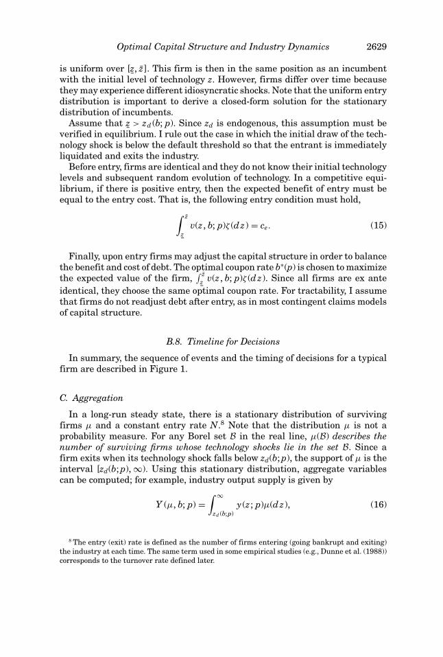
In the first step, I use the entry condition (15) to determine the equilibriumoutput price p∗. It is easy to show that firm value is strictly increasing in theoutput price. When the output price is high enough, expected firm value exceedsthe entry cost ce, and potential entrants have incentives to enter the industry.As more firms enter the industry, market competition drives down the outputprice. On the other hand, when the output price is low enough, expected firmvalue may be lower than the entry cost. In this case, no firm prefers to enterthe industry. In sum, if there is positive entry, the equilibrium output pricep∗ must be such that the expected firm value equals the entry cost, which isthe entry condition (15). To show that there is a unique solution p∗ to (15),observe the following: As price p goes to infinity, the firm makes unboundedprofits and hence firm value goes to infinity. However, as p goes to zero, the firmbecomes unprofitable so that it is abandoned and firm value goes to zero. Thus, aunique equilibrium output price p∗ is determined using the intermediate valuetheorem, as illustrated in Figure 2.

In the second step, I solve for the invariant distribution µ∗. I first solve forthe exit threshold and the support of µ∗. Given the equilibrium output price p∗,the equilibrium exit threshold ze = zd(b; p∗) is determined using equation (30).This threshold value is exactly analogous to the corresponding formula for thesingle-firm liquidation decision described in Section II. The intuition is similarto that discussed in Dixit and Pindyck (1994, Chapter 8). When uncertainty isfirm-specific, a firm that observes a favorable shock z has an edge over its com-petitors. Its favorable z cannot be “stolen” by competitors. Thus, a positive valueof waiting does survive, and the standard single-firm option value analysis canbe embedded in an industry equilibrium model.

Since inefficient firms with technology levels lower than ze exit the industry,the support of the stationary distribution of incumbents µ∗ is given by [ze, ∞).Note that equation (19) implies that µ∗ is linearly homogenous in the entryrate N∗. Thus, it is convenient to scale µ∗ by the factor N∗ when solving it.In Appendix A, I derive the scaled density of µ∗ using the method described inDixit and Pindyck (1994, Chapter 8). The main idea of this method follows fromthe intuitive description given in Section I.D. That is, in order for the densityto be constant over time, the rate at which firms arrive at any technology level


�p0

�

ce

∫ zz v(z, b; p)ζ(dz)

p∗

Figure 2. The determination of the equilibrium output price p∗. This figure illustratesthat the equilibrium output price p∗ is determined by the entry condition—the expected firm valueis equal to the entry cost.

because of entry must be equal to the rate at which firms move away from thatlevel because of Poisson deaths or bankruptcy.

In the final step, the entry rate N∗ is determined by the market-clearingcondition (18). Since the stationary distribution µ∗ is proportional to the entryrate N∗, it follows from (16) that industry output supply Y(µ∗, b; p∗) is alsoproportional to N∗. Equating the industry demand p∗ = Y(µ∗, b; p∗)−1/ε yieldsthe entry rate N∗.

B. Equilibrium with Endogenous Leverage

When each firm chooses a value-maximizing capital structure, it selects thecoupon rate b∗(p) to solve problem (34). The equilibrium output price po is thenthe solution to the following equation derived from the entry condition:∫ z̄

z¯

v(z, b∗(p); p)ζ (dz) = ce. (42)

Now, the equilibrium with endogenous leverage can be characterized in thesame manner as that with exogenous leverage except for the following changes:(i) The output price p∗ is replaced by the above value po; (ii) the coupon rateb takes the value bo ≡ b∗(po); and, (iii) the exit threshold ze takes the valuezo

e = ze(bo; po). The detailed computation of the equilibrium (bo, po, zoe , No, µo) is

described in Appendix B.


Importantly, if there is no fixed operating cost (i.e., cf = 0), then the equi-librium with endogenous leverage can be characterized completely in closedform.

PROPOSITION 6: Let Assumptions (39)–(41) hold. Also assume cf = 0. Then theunique stationary equilibrium with optimal leverage (po, zo

e , No, µo) is charac-terized as follows:

zoe =

[γ − ϑ

γ− ϑ(1 − α)

(1 − τ

)γ τ

] 1ϑ

[∫ z̄

z¯

zϑζ (dz)

] 1ϑ

, (43)

po = (ce)1γ

{(1 − ν)

(ν

r/(1 − τ ) + δ

)νγ [1 − τ

λ

z̄γ+1 − z¯γ+1

(z̄ − z¯)(γ + 1)

+ τ

λ

(zo

e

)γ

]}− 1γ

, (44)

No = (po)−(ε+γ ν)(∫ ∞

ze

zγ f o(z) dz)−1 (

ν

r/(1 − τ ) + δ

)−νγ

, (45)

where Nof o is the density of the stationary distribution µo and its explicit ex-pression is given in the appendix. Moreover, the optimal coupon rate is givenby

bo = (ϑ − γ )(r + η)a(po)ϑλ

[γ − ϑ

γ− ϑ(1 − α)

(1 − τ

)γ τ

] γ

ϑ[∫ z̄

z¯

zϑζ (dz)

] γ

ϑ

. (46)

Equation (43) implies that the exit threshold does not depend on the equi-librium output price. This result does not hold true if there are positive fixedoperating costs. In fact, when there are positive fixed costs, the equilibriumoutput price has an important feedback effect on the exit threshold and henceon the production and financing decisions, as illustrated in the simulationsbelow. Note that equation (44) implies that the equilibrium output price in-creases with entry cost. Although it is often argued that the entry cost shouldnot play a role in subsequent price competition, as it is a sunk cost, the presentmodel demonstrates that this sunk cost may feed back into the entry rate andconsequently in the output price. In particular, a high entry cost discouragesentry and hence protects incumbents. Thus, competition is less intense and theoutput price becomes higher.

To close this section, I introduce the concept of turnover rate. The turnoverrate is an important measure of industry dynamics (see Dunne, Roberts, andSamuelson (1988) and Hopenhayn (1992a)). The turnover rate of entry is de-fined as the ratio of the mass of entrants to the mass of incumbents. Theturnover rate of exit can be defined similarly. Since in a stationary equilib-rium the entry rate is equal to the exit rate, these two measures of turnoverare equal. Appendix B presents the explicit expressions for the turnover rateas well as other important equilibrium variables. In particular, the formula for


the turnover rate (B5) implies that the turnover rate is determined exclusivelyby the exit threshold and the scaled stationary distribution of firms.

IV. Results

To examine the implications of the model, I first calibrate a base case model. Ithen conduct simulations based on this model. For all simulations, input param-eter values are chosen such that the conditions of Proposition 5 are satisfied.

A. Parameter Values

The base case model studies the equilibrium with endogenous leverage de-scribed in Proposition 6. The parameter values are either taken from theestimated values from the data or chosen such that the model’s equilibriumbehavior matches some measured statistics as closely as possible. They areused as an illustrative benchmark. Some parameter values can be fine-tunedas in the real business cycle literature (e.g., Kydland and Prescott (1982)).

I first set the fixed operating cost cf = 0 so that there is a closed-form solutionto the unique equilibrium. I then set the price elasticity of demand ε = 0.75.

This number is within the range estimated by Phillips (1995).Next, I calibrate parameters related to technology. Set the returns-to-scale

parameter ν = 0.40, as estimated by Caballero and Engel (1999). This impliesγ = 1/(1 − ν) = 1.667. As in the business cycle literature, set the depreciationrate of capital δ = 0.1. In order to calibrate the drift µz and volatility σ z, useπ (zt; p) to proxy a firm’s cash flow. The growth rate and volatility of cash flowsare roughly equal to 2.5% and 25%, respectively, for a typical Standard & Poor’s500 firm. Thus, apply Ito’s Lemma to equation (3) to derive that σz = 0.25/γ =15% and µz = (0.025 − 0.5γ (γ − 1)σ 2

z )/γ = 0.75%Set the risk-free r = 5.22% so that it is equal to the average rate on Treasury

bills, as reported in Standard & Poor’s The Outlook in 2001. Set the corporatetax rate τ = 34%, as estimated by Graham (1996). Set the bankruptcy cost pa-rameter 1 − α = 20%, which is at the upper bound of recent estimates reportedin Andrade and Kaplan (1998).

Set the Poisson death parameter η = 4%. This number follows from the factsthat the annual turnover rate is roughly 7% (see Dunne et al. (1988) andHopenhayn (1992b)) and that the default rate is roughly 3% (see Brady andBos (2002)).

It remains to calibrate the parameters ce, z¯, and z̄. First, follow Hopenhayn

(1992b) and normalize the equilibrium output price po = 1. Next, useequation (42) to determine ce once z

¯and z̄ are known. Finally, choose val-

ues for z¯

and z̄ so that the following numbers are roughly matched: (i)The average industry Tobin’s q is equal to 2.7, which is in the rangeestimated by Lindenberg and Ross (1981); and, (ii) the turnover rate is7%.

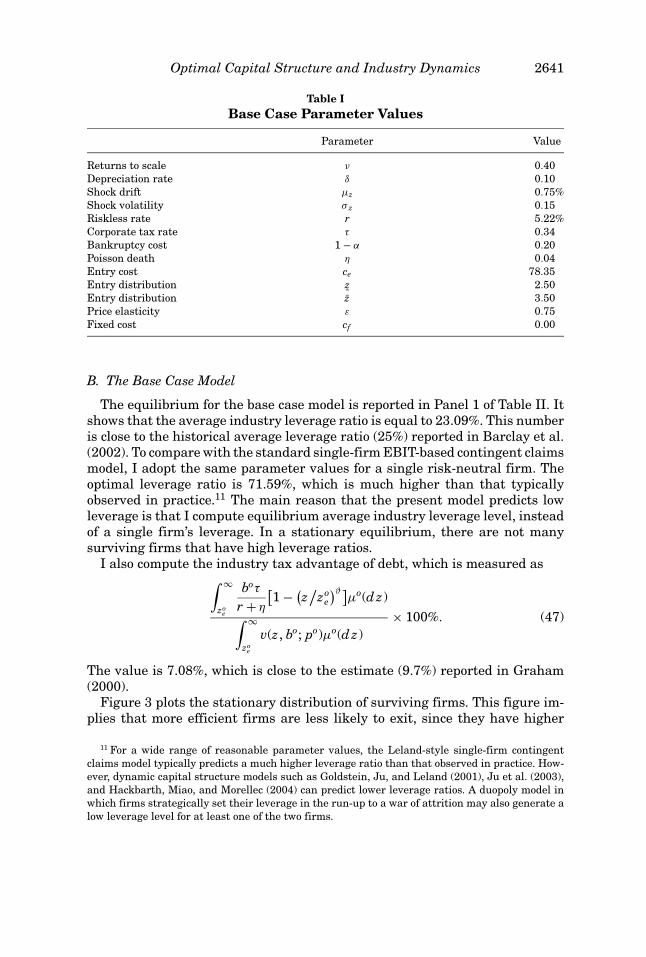
The base case parameter values are summarized in Table I.


Table IBase Case Parameter Values

Parameter Value

Returns to scale ν 0.40Depreciation rate δ 0.10Shock drift µz 0.75%Shock volatility σ z 0.15Riskless rate r 5.22%Corporate tax rate τ 0.34Bankruptcy cost 1 − α 0.20Poisson death η 0.04Entry cost ce 78.35Entry distribution z

¯2.50

Entry distribution z̄ 3.50Price elasticity ε 0.75Fixed cost cf 0.00

B. The Base Case Model

The equilibrium for the base case model is reported in Panel 1 of Table II. Itshows that the average industry leverage ratio is equal to 23.09%. This numberis close to the historical average leverage ratio (25%) reported in Barclay et al.(2002). To compare with the standard single-firm EBIT-based contingent claimsmodel, I adopt the same parameter values for a single risk-neutral firm. Theoptimal leverage ratio is 71.59%, which is much higher than that typicallyobserved in practice.11 The main reason that the present model predicts lowleverage is that I compute equilibrium average industry leverage level, insteadof a single firm’s leverage. In a stationary equilibrium, there are not manysurviving firms that have high leverage ratios.

I also compute the industry tax advantage of debt, which is measured as∫ ∞

zoe

boτ

r + η

[1 − (

z/

zoe

)ϑ]µo(dz)∫ ∞

zoe

v(z, bo; po)µo(dz)× 100%. (47)

The value is 7.08%, which is close to the estimate (9.7%) reported in Graham(2000).

Figure 3 plots the stationary distribution of surviving firms. This figure im-plies that more efficient firms are less likely to exit, since they have higher

11 For a wide range of reasonable parameter values, the Leland-style single-firm contingentclaims model typically predicts a much higher leverage ratio than that observed in practice. How-ever, dynamic capital structure models such as Goldstein, Ju, and Leland (2001), Ju et al. (2003),and Hackbarth, Miao, and Morellec (2004) can predict lower leverage ratios. A duopoly model inwhich firms strategically set their leverage in the run-up to a war of attrition may also generate alow leverage level for at least one of the two firms.


Table IIComparative Statics for Selected Parameter Values

The parameter values for the base case model are given in Table I. Comparative statics is basedon the base case model. When performing simulations for the entry cost and demand elasticity, Iset the fixed cost cf = 5.

Industry Industry Average Turnover Exit Optimal AgencyOutput Price Leverage (%) Rate (%) Threshold Coupon Cost (%)

Base case 1.00 1.00 23.09 7.51 1.91 6.66 2.57

µz = 0.5% 0.97 1.04 28.12 7.73 1.89 6.70 3.37µz = 1.0% 1.03 0.96 17.50 7.29 1.92 6.62 1.80µz = 1.5% 1.10 0.88 4.46 6.91 1.94 6.55 0.39

σz = 10% 0.97 1.04 39.43 6.04 2.04 6.28 2.76σz = 15% 1.00 1.00 23.09 7.51 1.91 6.66 2.57σz = 20% 1.06 0.92 7.04 9.13 1.79 7.18 1.08

z̄ = 3.5 1.00 1.00 23.09 7.51 1.91 6.66 2.57z̄ = 4.0 1.06 0.92 22.42 7.46 2.03 6.49 2.42z̄ = 4.5 1.12 0.86 21.68 7.40 2.15 6.30 2.25

α = 95% 1.01 0.998 24.50 8.27 2.02 7.20 2.51α = 90% 1.006 0.992 24.00 7.98 1.98 7.01 2.54α = 80% 1.00 1.00 23.09 7.51 1.91 6.66 2.57

τ = 25% 1.04 0.95 20.43 7.12 1.84 5.96 1.74τ = 34% 1.00 1.00 23.09 7.51 1.91 6.66 2.57τ = 40% 0.97 1.04 25.00 7.70 1.94 7.08 3.22

cf = 5 0.82 1.31 16.64 9.37 2.15 7.77 1.77cf = 10 0.72 1.55 13.54 10.83 2.27 8.48 1.30cf = 12 0.69 1.64 12.68 11.35 2.30 8.76 1.17

ce = 70 0.85 1.25 16.16 9.55 2.16 6.94 1.70ce = 85 0.80 1.35 16.97 9.24 2.13 8.23 1.82ce = 100 0.76 1.44 17.61 9.01 2.11 9.52 1.92

ε = 0.60 0.85 1.31 16.64 9.37 2.15 7.66 1.77ε = 0.75 0.82 1.31 16.64 9.37 2.15 7.66 1.77ε = 0.90 0.79 1.31 16.64 9.37 2.15 7.66 1.77

η = 0.03 1.07 0.91 10.04 6.16 1.89 5.99 1.12η = 0.04 1.00 1.00 23.09 7.51 1.91 6.66 2.57η = 0.05 0.94 1.08 31.35 8.80 1.92 7.33 3.46

technology (productivity) levels that are farther away from the exit threshold.This prediction is consistent with the empirical finding reported by Kovenockand Phillips (1997). Since the size of a firm measured by either output y(z,p)or input k(z, p) is an increasing function of its technology shock z, the long-runsize (probability) distribution plotted in Figure 4 has a similar shape to thatplotted in Figure 3. Note that the size distribution does not depend on firm age.The issue of size and age dependence is studied by Cooley and Quadrini (2001).

Another property of the base case model is that although all firms in theindustry are ex ante identical, and hence pay the same coupon amount, the


1 2 3 4 5 6 7 8 9 10 110

1

2

3

4

5

6

Technology shock z

Sca

led

dens

ity f

Figure 3. The effect of an increase in growth of technology on the scaled density of firms.The solid line is for the base case model. The dashed line is for µz = 1.5%. All other parameter valuesare given in Table I.

leverage ratios vary across firms. In particular, small or inefficient firms takeon high leverage. This is because surviving firms differ in realizations of tech-nology shocks so that they have different equity values.12 This result is relatedto the empirical finding of Welch (2004) that leverage changes are mainly de-termined by equity returns.

Simulations reported in Table II also reveal that the average industry agencycost accounts for 2.57% of the first–best average industry firm value. In latersimulations, I find that the magnitude of the average industry agency costis approximately 2% for a wide range of parameter values. Thus, the agencycosts arising from the conflict of interest between shareholders and bond-holders are quite small. A similar finding is reported in Parrino and Weis-bach (1999). The present model implies that competition can mitigate thebondholder–shareholder agency problem. This is because inefficient firms have

12 Maksimovic and Zechner (1991) attribute the variation of capital structures to the adoptionof different technologies within the industry.


5 10 15 20 25 30 350

0.05

0.1

0.15

0.2

0.25

0.3

0.35

0.4

0.45

Output y

Siz

e di

strib

utio

n

Figure 4. The size distribution of firms. This figure plots the size distribution of firms mea-sured according to output. This distribution is derived from the scaled density of the equilibriumstationary distribution. The parameter values are given in Table I.

high agency costs as discussed in Section II.E, but they cannot survive in anindustry equilibrium.

To compare with Hopenhayn’s (1992a) industry dynamics model without debtfinancing, I set the fixed operating cost cf = 5 and compute equilibria withand without debt financing. The equilibrium outcome for the model with debtfinancing is reported in the 12th row of Table II. By contrast, when firms do nottake into account tax advantages of debt and are all-equity financed, industryoutput is 0.72, the turnover rate is 4.77%, and average industry firm valueis 372.12, all of which are lower than the model with debt financing. Thus,debt financing not only raises firm value,13 but also facilitates efficient exitand increases industry output. The intuition is simple. Debt increases the exitthreshold (see equations (26) and (30)), and hence induces inefficient firms toexit. In addition, increased firm value promotes entry. Competition then drivesdown the output price and raises industry output.

13 Average industry firm value is 395.57 in the present model. This number is not reported inTable II.


C. Comparative Statics

Since capital structure and production decisions may simultaneously respondto changes in exogenous factors, I focus on the stationary equilibrium withoptimal leverage described in Section III.B and examine comparative staticproperties of the equilibrium based on the base case model studied earlier.

C.1. Technology Growth and Entry Distribution

Panel 2 of Table II details the effect of changes in technology growth. Asargued in the introduction, the standard single-firm tradeoff model cannot ex-plain the empirical evidence that high growth firms have low leverage. How-ever, in the present industry equilibrium framework, the tradeoff theory canstill explain this fact. This is because the price feedback effect discussed in theintroduction plays an important role. Simulations reported in Table II showthat this effect dominates so that the optimal coupon rate falls and the liqui-dation threshold rises with technology growth µz. Simulations also reveal thatthe tax benefit of debt falls and average industry leverage falls with µz.

Since the market-to-book ratio is positively related to technology growth,14 itis negatively related to leverage. The usual interpretation of this fact is based onthe underinvestment problem of debt identified by Myers (1977) or the free cashflow theory of Jensen (1986). Two recent interpretations are offered by Welch(2004) and Baker and Wurgler (2002). The present model, however, offers a newinterpretation in an industry equilibrium setting.

To examine why the price feedback effect may dominate and how robust theresult is, consider the expression for the before-tax present value of profits (25),

�(z; p) =pγ (1 − ν)

(ν

r/(1 − τ ) + δ

)νγ

r + η − µzγ − σ 2z γ (γ − 1)

/2

zγ − c f

r + η, (48)

where I have substituted the expressions for a(p) and λ in (8) and (22). If � (z;p) is price elastic (i.e., γ > 1), and if the level and changes of the growth rateµz are small, then the decrease in the price p may well dominate the increasein µz. In the present model, under decreasing-returns-to-scale technology ν <

1, γ ≡ 1/(1 − ν) must be bigger than 1. Moreover, for a typical firm the growthrate of cash flows and its change are unlikely to be high. Therefore, I concludethat the result is quite robust for a wide range of reasonable parameter values.

The increase in µz also has a positive selection effect because it changesthe liquidation threshold and the stationary distribution of firms. Figure 3illustrates that this effect causes the scaled density function to shift to theright. Thus, to survive in the industry, firms must have high productivity ortechnology levels. This makes entry tougher. Thus, the turnover rate decreases.

14 Simulations (not reported in Table II) confirm this positive correlation. The market-to-bookratio is a commonly used proxy for growth opportunities.


Note that even though the increase in technology growth may cut the presentvalue of profits, the average industry equity value and firm value rise with tech-nology growth. Simulations show that when µz increases from 0.75% to 1.5%,average industry equity value increases from 203.57 to 1338.2 and average in-dustry firm value increases from 264.68 to 1400.8. This is because those valuesare computed using the stationary distribution of surviving firms. In addition,the positive selection effect implies that a high growth industry has a greaternumber of highly efficient firms than a low growth industry. These highly effi-cient firms have higher equity value and firm value. Furthermore, simulationsshow that the size of the high growth industry is much lower than that of thelow growth industry.

The impact of an improvement of the entry distribution (i.e., an increase inz̄) is similar to that of an increase in technology growth, as reported in Panel 4of Table II. So I omit the discussion.

C.2. Riskiness of Technology

Panel 3 of Table II documents the effect of changes in technology volatility. Asin the standard contingent claims model, the volatility parameter σ z provides ameasure of bankruptcy risk and hence is an important determinant of leverage.Panel 3 of Table II reveals that volatility is negatively related to average in-dustry leverage. This prediction is similar to that in the single-firm model andis consistent with the empirical evidence documented by Titman and Wessels(1988).

Panel 3 of Table II also reveals that volatility is positively related to indus-try output. This is because an increase in σ z has an option effect in that itraises the option value of waiting to default. This results in higher firm valueand hence encourages entry. Competition then drives down the output priceand raises industry output. Finally, Panel 3 of Table II reveals that an in-crease in volatility has a positive selection effect, resulting in a high turnoverrate.

C.3. Bankruptcy Cost and Corporate Tax

Panel 5 of Table II reports the effect of changes in the bankruptcy cost. Anincrease in the bankruptcy cost parameter 1 − α has a negative cash flow effect.This effect decreases the value of an active firm and depresses entry. As a result,the output price rises and industry output falls.

While it is intuitive that bankruptcy costs are negatively related to leverage,Panel 5 of Table II also reveals that bankruptcy costs are negatively related tothe turnover rate. The intuition is that an increase in the bankruptcy cost low-ers debt and hence decreases the opportunity cost of remaining active. Thus,each incumbent prefers to stay longer in the industry. Consequently, the liqui-dation threshold falls. The lower value of the liquidation threshold implies lessselection and higher expected lifetime of firms. As a result, the turnover ratefalls.


An increase in the corporate tax rate has the same negative cash flow effectas an increase in the bankruptcy cost so that industry output falls with thetax rate. However, the increase in the corporate tax rate raises the tax benefitof debt and hence has an opposite effect on leverage and turnover relative toan increase in the bankruptcy cost. The impact of the tax rate is reported inPanel 6 of Table II. I omit the detailed analysis.

C.4. Fixed Operating Cost

So far, I have set the fixed operating cost cf to zero. Because the fixed cost isrelated to the degree of economies of scale, I now examine the impact of the fixedoperating cost on equilibrium outcomes, as reported in Panel 7 of Table II.15

The panel reveals that the fixed cost is positively related to the turnoverrate, and negatively related to industry output and leverage. The intuition isas follows. An increase in the fixed operating cost lowers the operating profitand hence lowers firm value. This depresses entry, raises the output price, andhence lowers industry output. As reported in Panel 7 of Table II, the positiveprice feedback effect is dominated so that each incumbent prefers to exit earlier,resulting in an increased exit threshold and an increased turnover rate.

I now analyze the impact on leverage. While the increased fixed cost lowersthe tax benefit of debt, it also lowers unlevered firm value and hence bankruptcycosts. Simulations reported in Panel 7 of Table II reveal that the latter effectdominates so that the optimal coupon rises. Thus, the average industry value ofdebt also rises. However, due to the positive selection and price effects, averageindustry firm value also increases with the fixed cost. The intuition is that fol-lowing an increase in the fixed cost, surviving firms are more efficient since theexit threshold is higher and the positive price effect is stronger for those firms.A similar result is derived in Hopenhayn (1992a, 1992b) for all-equity financedfirms. Simulations reported in Panel 7 of Table II show that the increase in firmvalue dominates the increase in debt value so that average industry leveragefalls with the fixed cost.

C.5. Entry Cost

In the short run, an increase in the entry cost ce does not affect a firm’s cashflows and its liquidation decision. Thus, it does not affect the value of an activefirm. However, the entry cost acts as a barrier to entry. High entry costs protectincumbents and drive up the industry output price. This price feedback effectwill generally influence financing and exit decisions.

Specifically, the increase in the output price raises the benefit of remain-ing active and the tax advantage of debt. On the other hand, this impliesthat each firm prefers to issue more debt and hence the optimal couponrises. This leads to an increased opportunity cost of remaining active. The

15 As a robustness check, I redo all previous simulations for a number of positive values of theentry cost. I find the results do not change qualitatively.


impact on the exit threshold depends on these two opposite effects as shownin equation (31). When there is no fixed operating cost, these effects offseteach other so that changes in the entry cost do not affect the exit thresh-old (see equation (43)). Consequently, these changes do not have a selectioneffect.

However, this result is not robust to the introduction of the fixed operatingcost. To illustrate this point, I set the operating cost cf = 5. Panel 8 of Table IIdocuments the impact of increases in the entry cost. It reveals that the entry costis positively related to leverage and negatively related to the turnover rate.16

This is because in response to an increase in the entry cost, the positive pricefeedback effect dominates so that the exit threshold decreases. This results ina negative selection effect so that the turnover rate falls. This prediction isconsistent with the evidence reported by Orr (1974) for Canadian industry. Asimilar result is derived by Hopenhayn (1992a) for all-equity financed firms.In the present model, a lower exit threshold also induces lower default/exitprobabilities, and hence expected bankruptcy costs are lower. This results inhigher leverage.

C.6. Industry Demand Elasticity

I now analyze the impact of changes in demand elasticity, which is an impor-tant industry characteristic. From Proposition 6, one finds surprisingly that theoutput price po, the exit threshold zo

e , and the scaled density f o do not dependon the demand elasticity parameter ε. Consequently, the turnover rate and av-erage industry leverage do not depend on ε. However, the change in demandelasticity does have on effect an industry output, industry size, and entry rate.As can be seen from Appendix B, this result is also true for positive fixed costscf > 0. The key intuition is that the competitive entry condition (15), which de-termines the equilibrium output price, is independent of the industry demandelasticity. This implies that the industry output price is also independent ofthe demand elasticity. Consequently, the exit threshold is independent of thedemand elasticity since it is determined by an individual firm’s behavior takingindustry prices as given. Since the scaled stationary distribution is determinedby the exit threshold and the exogenous evolution of the technology process, itis also independent of the demand elasticity.

To illustrate the above result, I set cf = 5 and fix other parameter valuesas in Table I. Panel 9 of Table II illustrates the effect of increases in the de-mand elasticity. I find that the industry output, industry size, and entry rateall decrease. This is because the isoelastic demand function (1) implies that theindustry output decreases with the demand elasticity for any fixed price p > 1.To accommodate decreased industry output, the entry rate and industry sizemust fall.

16 This result does not depend on the choice of cf = 5 since it is verified by simulations for manyother values of cf .


C.7. Poisson Deaths

As discussed earlier, a sufficiently high Poisson death rate is needed for theexistence of a stationary equilibrium in the present model. I now examine theimpact of changes in this rate, as detailed in the last panel of Table II. Asexpected, increased death rates lower industry output. Surprisingly, firms is-sue more debt and average industry leverage increases. This is because anincumbent enjoys high output price and hence high tax benefits of debt (seeequation (36)). Consider next the turnover rate. In order for the population offirms to keep being refreshed, the turnover rate of entry must rise in responseto an increased Poisson death rate. Surprisingly, the turnover rate of exit dueto bankruptcy also rises, which is the difference between the turnover rate ofentry and the Poisson death rate.17 This is because the exit threshold rises fol-lowing an increase in the Poisson death rate. Thus, firms are more likely to gobankrupt and exit.

V. Conclusion

In this paper, I present a competitive equilibrium model of industry dynamicsand capital structure decisions. I show that technology (productivity) hetero-geneity is important in determining a firm’s survival probability and leverageratio. In particular, in equilibrium there is a stationary distribution of survivingfirms. These firms exhibit a wide variation of capital structures. In addition,more efficient firms are less likely to exit and have lower agency costs. Finally,I analyze comparative static properties of changes in technology growth, tech-nology risk, entry distribution, entry cost, fixed cost, bankruptcy cost, and taxpolicy.

The analysis reveals that the interaction between financing and productiondecisions is important in an industry equilibrium. Moreover, the equilibriumoutput price has an important feedback effect. As a result, several conclusionsreached in the standard single-firm contingent claims models do not hold true inan equilibrium setting. Moreover, it moves predictions in the right direction interms of reconciling the empirical evidence. Specifically, the analysis shows thateither one of the following exogenous factors can simultaneously explain theempirical findings mentioned in the introduction: the slowdown of technology(productivity) growth, the deterioration of entry distribution, or the increase inthe corporate tax rate.

The paper also provides a number of new testable predictions regarding cap-ital structure and industry dynamics. First, industries with high technologygrowth or good starting distributions of technology have relatively lower aver-age leverage, lower turnover rates, and higher output. Second, industries withrisky technology have relatively lower average leverage, higher turnover rates,and higher output. Third, industries with high bankruptcy costs have rela-tively lower average leverage, lower turnover rates, and lower output. Fourth,

17 This rate is given by 3.16, 3.51, and 3.80 for η equal to 0.03, 0.04, and 0.05, respectively.


industries with high fixed operating costs have relatively lower average lever-age, higher turnover rates, and lower output. Finally, industries with high entrycosts have relatively higher average leverage, lower turnover rates, and loweroutput.

The paper could be extended in several directions, which are left for futureresearch. First, in the paper, the expected returns of equity and other macroe-conomic variables are constant. To study equity premium and other time-seriesbehavior of the industry, it is necessary to introduce aggregate uncertainty. Sec-ond, this paper considers only the conflict of interest between shareholders andbondholders. It would be interesting to study the conflict of interest betweenshareholders and managers. Third, I analyze firms’ initial capital structuredecisions only, as in most contingent claims models of capital structure in theliterature. A model of dynamic capital structure would be worth pursuing (Le-land (1998), Goldstein, Ju, and Leland (2001), Ju et al. (2003), and Hackbarth,Miao, and Morellec (2004)). Finally, it would be interesting to consider finitematurity debt. This requires a constant default threshold in stationary equi-librium, which can be delivered using the framework of Leland and Toft (1996)or Leland (1998).

Appendix A. Proofs

Proof of Propositions 1–2:18 I first prove Proposition 2. Proposition 1 is ob-tained by setting b = 0. It follows from (27) that equity value given a defaultthreshold y is given by

e(z, b; p | y) = (1 − τ )Ez[∫ Ty

0e−(r+η)t(π (zt ; p) − b) dt

]. (A1)

This expression is equal to

(1 − τ )Ez[∫ ∞

0e−(r+η)t(π (zt ; p) − b) dt

]− (1 − τ )Ez

×[∫ ∞

Ty

e−(r+η)t(π (zt ; p) − b) dt

]= (1 − τ )Ez

[∫ ∞

0e−(r+η)t(π (zt ; p) − b) dt

]

− (1 − τ )E y[∫ ∞

0e−(r+η)t(π (zt ; p) − b) dt

]× Ez[e−(r+η)Ty

], (A2)

where the last equality follows from the strong Markov property of the process(zt)t≥0 (see Karatzas and Shreve (1991, p. 82)). By an argument similar to thatin Karatzas and Shreve (1991, p. 197),

Ez[e−(r+η)Ty] =

(zy

)ϑ

, (A3)

18 Here I use a probabilistic proof method similar to Mella-Barral (1995) and Morellec (2004).An alternative standard method is to use ODEs (e.g., Leland (1994)).


where ϑ is given in (24). Substitute this expression into above equations toderive

e(z, b; p | y) = (1 − τ )

[�(z; p) − b

r + η+

(b

r + η− �( y ; p)

) (zy

)ϑ]

. (A4)

Use the smooth-pasting condition (28) to derive the optimal default thresholdzd(b; p) in (30). Use the fact that e(z, b; p) = e(z, b; p | zd) to derive equity valuein (29). Q.E.D.

Proof of Proposition 3: As in the proof of Propositions 1–2, one can use (13)and the strong Markov property to derive

d (z, b; p)

= Ez[∫ Tzd

0e−(r+η)t bdt


]

= Ez[∫ ∞

0e−(r+η)t bdt

]− Ez

[∫ ∞

Tzd

e−(r+η)t bdt


]

= br + η

− Ez[∫ ∞

0e−(r+η)t bdt

]Ez[e−(r+η)Tzd

] + αA(zd ; p)Ez[e−(r+η)Tzd

]

= br + η

+(

αA(zd ; p) − br + η

)Ez[e−(r+η)Tzd

]. (A5)

Use the last expression and (A3) to obtain (32). Finally, one can derive firmvalue in (33) by using equations (13), (29), and (32). Q.E.D.

Proof of Proposition 4: Similar to the derivation of equation (33), one candeduce that firm value given a default threshold y is given by

v(z, b; p | y) = A(z; p) + bτ

r + η

[1 −

(zy

)ϑ]

− (1 − α)A( y ; p)(

zy

)ϑ

. (A6)

The first–best liquidation policy is to choose default threshold y so as to maxi-mize firm value in (A6). It can be verified that the maximizer is zFB

d = zA. Equa-tion (37) follows from the fact that vFB(z, b; p) = v(z, b; p | zA). Finally, equation(38) follows from cA(z, b; p) = vFB(z, b; p) − v(z, b; p). Q.E.D.

Proof of Proposition 5: As argued in Section III.A, the proof consists of threesteps. In the first step, one uses the entry condition to solve for the equilibriumoutput price p∗. Then the exit threshold ze is determined by ze = zd(z, b; p∗) usingequation (30). In the second step, one solves for the density f of the stationarydistribution µ∗ up to a scale factor N∗. In the final step, the entry rate N∗ isdetermined by the market-clearing condition (18). Specifically, use (5) and (16)to derive the industry output


Y (µ∗, b; p∗) = N ∗∫ ∞

ze

zγ f (z) dz(

pν

r/(1 − τ ) + δ

)νγ

. (A7)

Use the market-clearing condition p∗ = Y(µ∗, b; p∗)−1/ε to derive the entry rate

N ∗ = (p∗)−(ε+γ ν)(∫ ∞

ze

zγ f (z)dz)−1 (

ν

r/(1 − τ ) + δ

)−νγ

. (A8)

Note that the integral∫ ∞

zezγ f (z) dz is improper since the density f has an

infinite support. Once f is derived toward the end of the proof, one will see thatassumption (40) ensures that this improper integral is finite.

The remainder of the proof is devoted to the second step, which is key. Itis convenient to work in terms of the logarithm, x = log z. Then (xt)t≥0 is aBrownian motion satisfying,

dxt = µx dt + σx dWt , (A9)

where µx = µz − 12σ 2

z and σx = σz. Because the initial draw of z is uniform over[z¯, z̄], the initial draw of x = log (z) has an exponential distribution over [x

¯, x̄],

where x̄ = log z̄ and x¯

= log z¯. This distribution has a density function

g (x) = exp(x − x̂), (A10)

where x̂ = log(z̄ − z¯).

Let the stationary distribution of incumbent firms have a density functionN∗φ(x) on [xe, ∞), where xe = log (ze) and N∗ is the entry rate determined later.I will now use the Kolmogorov equation to find the function φ(x) by consideringthree cases.

I adapt the heuristic argument from Dixit and Pindyck (1994, Chapter 8).First, approximate the Brownian motion by a random walk. To do so, dividetime into short intervals of duration dt, and the x space into short segments,each of length dh = σx

√dt. Of the firms located in one such segment, during

time dt a proportion η dt will die. Of the rest, a fraction qr will move one segmentto the right, and a fraction ql will move to the left, where

qr = 12

[1 + µx

σx

√dt

], ql = 1

2

[1 − µx

σx

√dt

]. (A11)

Now consider the first case, where x¯

≤ x < x̄. Then there are new entrantsthat realize shock x since the support of their initial draw of shocks is [x

¯, x̄].

There are N∗φ(x) dh firms in the segment centered at x. In the next unit oftime period dt, all of these firms move away with either Poisson or Brownianshocks. New entrants, as well as firms from the left and right, arrive to taketheir places. For balance,

N ∗φ(x) dh = N ∗dt g (x) dh + qr (1 − η dt)N ∗φ(x − dh) dh

+ ql (1 − η dt)N ∗φ(x + dh) dh. (A12)


Apply Taylor’s expansion theorem and simplify to obtain the ODE

12

σ 2x φ′′(x) − µxφ

′(x) − ηφ(x) + g (x) = 0. (A13)

A particular solution to this equation can be derived as

φ0(x) = ex−x̂/(η + µx − σ 2

x

/2). (A14)

To make economic sense, this density must be positive (also see Dixit andPindyck (1994, p. 275)). This is ensured by assumption (41) since η + µx −σ 2

x /2 = η + µz − σ 2z > 0. The general solution to (A13) is given by

φ(x) = A1eβ1x + A2eβ2x + φ0(x), for x¯

≤ x < x̄, (A15)

where

β1 = µx − √µ2

x + 2σ 2x η

σ 2x

, β2 = µx + √µ2

x + 2σ 2x η

σ 2x

, (A16)

and A1 and A2 are constants to be determined.In the second case, xe < x < x

¯, there is no new entrant in the segment centered

at x. Apply a similar method to show that φ satisfies the following ODE:

12

σ 2x φ′′(x) − µxφ

′(x) − ηφ(x) = 0. (A17)

The general solution to this equation is given by

φ(x) = G1eβ1x + G2eβ2x , for xe < x < x¯, (A18)

where G1 and G2 are constants to be determined.In the third case, x ≥ x̄, there is no new entrant in the segment centered at

x, so φ still satisfies the above ODE. Let the solution be

φ(x) = H1eβ1x + H2eβ2x , for x ≥ x̄, (A19)

where H1 and H2 are constants to be determined.The constants A1, A2, G1, G2, H1, and H2 are determined by the following six

boundary conditions: ∫ ∞

x̄φ(x) dx < ∞, (A20)

φ(xe) = 0, (A21)

limx↑x

¯φ(x) = lim

x↓x¯

φ(x), (A22)

limx↑x

¯φ′(x) = lim

x↓x¯

φ′(x), (A23)

limx↑x̄

φ(x) = limx↓x̄

φ(x), (A24)


limx↑x̄

φ′(x) = limx↓x̄

φ′(x). (A25)

Equation (A20) says that the total mass of incumbents must be finite.Equation (A21) is derived from the fact that when the process (xt) falls toxe, the firm exits the industry. Finally, equations (A22)–(A25) follow fromTheorem 4.4.9 in Karatzas and Shreve (1991, p. 271). These equations ensuresufficient smoothness of φ. Using equations (A20)–(A25), one can derive H2 = 0and G1, G2, A1, A2, H1 solve the following system of linear equations:

G1eβ1xe + G2eβ2xe = 0,

G1eβ1x¯ + G2eβ2x

¯ = A1eβ1x¯ + A2eβ2x

¯ + φ0(x¯),

G1β1eβ1x¯ + G2β2eβ2x

¯ = A1β1eβ1x¯ + A2β2eβ2x

¯ + φ′0(x

¯),

A1eβ1 x̄ + A2eβ2 x̄ + φ0(x̄) = H1eβ1 x̄ ,

A1β1eβ1 x̄ + A2β2eβ2 x̄ + φ′0(x̄) = H1β1eβ1 x̄ . (A26)

The solution in terms of z is

A1 = (1 − β1)zβ2−β1e (z̄1−β2 − z

¯1−β2 ) + (1 − β2)z

¯1−β1

(β2 − β1)(z̄ − z¯)(η + µz − σ 2

z

) ,

A2 = − (1 − β1)z̄1−β2

(β2 − β1)(z̄ − z¯)(η + µz − σ 2

z

) ,

G1 = (1 − β1)zβ2−β1e (z̄1−β2 − z

¯1−β2 )

(β2 − β1)(z̄ − z¯)(η + µz − σ 2

z

) ,

G2 = (1 − β1)(z¯

1−β2 − z̄1−β2 )(β2 − β1)(z̄ − z

¯)(η + µz − σ 2

z

) ,

H1 = (1 − β1)zβ2−β1e (z̄1−β2 − z

¯1−β2 ) + (β2 − 1)(z̄1−β1 − z

¯1−β1 )

(β2 − β1)(z̄ − z¯)(η + µz − σ 2

z

) . (A27)

In terms of z, the density function of µ∗ is given by N ∗ f (z) = N ∗z φ(log(z)), where

f (z) =

G1zβ1−1 + G2zβ2−1, for ze < z ≤ z¯,

A1zβ1−1 + A2zβ2−1 + 1(z̄ − z

¯)(η + µz − σ 2

z

) , for z¯

< z ≤ z̄,

H1zβ1−1, for z > z̄.

(A28)

I finally show that assumption (40) ensures∫ ∞

zezγ f (z) dz is finite. It suffices

to show that∫ ∞

z̄ zγ f (z) dz is finite. Since f (z) = H1zβ1−1 for z > z̄,∫ ∞

z̄zγ f (z) dz = H1

∫ ∞

z̄zβ1+γ−1 f (z) dz = H1

β1 + γ

(limz→∞ zβ1+γ − z̄β1+γ

). (A29)


Thus, if and only if β1 + γ < 0 is satisfied, limz→∞ zβ1+γ = 0 and theabove integral is finite. By (A16), the condition β1 + γ < 0 is equivalent toassumption (40). Q.E.D.

Proof of Proposition 6: The analysis in Section II.D shows that when cf = 0,for any output price p the optimal coupon rate b∗(p) is given by (36). Sincecf = 0, it follows from (31) that the exit threshold is given by

zd (b; p) =[

ϑλb(ϑ − γ )(r + η)a(p)

]1/γ

. (A30)

Substituting (36) for b into this expression yields

zd (b∗(p); p) =[γ − ϑ

γ− ϑ(1 − α)(1 − τ )

γ τ

] 1ϑ

[∫ z̄

z¯

zϑζ (dz)

] 1ϑ

. (A31)

Since this expression is independent of the output price, it is also the equilib-rium exit threshold zo

e given in (43). I now derive the equilibrium output priceusing the entry condition (42). Substituting (33), (36), and (43) into (42), onecan solve for the unique equilibrium output price po given in (44). Finally, theequilibrium entry rate No is obtained from (A8) by replacing p∗ with po and thescaled density f o is obtained from (A28) by replacing ze with zo

e . Q.E.D.

Appendix B. Computation of Stationary Equilibrium

This appendix provides explicit formulas and an algorithm to compute thestationary equilibrium with endogenous leverage (bo, po, zo

e , No, µo) described inSection III.B for the case with positive fixed cost cf > 0. The algorithm consistsof the following steps:

Step 1. Solve for the optimal coupon rate bo and the equilibrium output pricepo using the system of two equations (34) and (41). Specifically, rewrite (34) and(41) in an explicit form

τ

r + η

[1 −

∫ z̄

z¯

(zzd

)ϑ

ζ (dz)

]= −ϑ

γ

τb(r + η)(b + c f )

∫ z̄

z¯

(zzd

)ϑ

ζ (dz)

+ 1 − α

γ (b + c f )[A′(zd ; p)zd − ϑ A(zd ; p)]

×∫ z̄

z¯

(zzd

)ϑ

ζ (dz), (B1)


ce =∫ z̄

z¯

A(z; p)ζ (dz) + bτ

r + η

[1 −

∫ z̄

z¯

(zzd

)ϑ

ζ (dz)

]

− (1 − α)A(zd ; p)∫ z̄

z¯

(zzd

)ϑ

ζ (dz). (B2)

Substituting the expressions for zA, zd, and A(z, p) in equations (25), (29), and(22), respectively, into the above two equations yields a system of two nonlinearequations for two unknowns, (b, p). Any standard nonlinear equation solver candeliver numerical solutions for (bo, po).

Step 2. Solve for the exit threshold zoe . Once (bo, po) is obtained, use (29) to

compute zoe = zd(bo; po).

Step 3. Solve for the scaled density f o of the stationary distribution µo. Theexpression for f o is the same as that given in (A28), but ze must be replaced byzo

e in the support and also in the coefficients A1, A2, G1, G2, and H1.Step 4. Solve for the entry rate No. The expression for No is the same as that

given in (A8), but p∗ must be replaced by po.The expressions for other important equilibrium variables are described as

follows:

1. Industry output. Use the industry demand (1) to derive

Y (µo, bo; po) = (po)−ε. (B3)

2. Turnover rate. It is defined as the ratio of the entry rate to the mass ofincumbents. Since the mass of incumbents (size of the industry) is givenby

M o =∫ ∞

zoe

µo(dz) = No∫ ∞

zoe

f o(z) dz, (B4)

the turnover rate No/Mo is given by

No

M o = 1∫ ∞

zoe

f o(z) dz. (B5)

3. Average industry agency costs. The absolute value is defined as the totalindustry agency costs divided by the mass of incumbents

1M o

∫ ∞

zoe

cA(z, bo; po)µo(dz) = No

M o

∫ ∞

zoe

cA(z, bo; po) f o(z) dz. (B6)

The relative value is defined as the percentage of the average industryfirst–best firm value


1M o

∫ ∞

zoe

cA(z, bo; po)µo(dz)

1M o

∫ ∞

zoe

vF B(z, bo; po)µo(dz)=

∫ ∞

zoe

cA(z, bo; po) f o(z) dz∫ ∞

zoe

vF B(z, bo; po) f o(z) dz. (B7)

4. Average industry leverage. It is defined as the ratio of the average industrydebt value to the average industry firm value:

1M o

∫ ∞

zoe

d (z, bo; po)µo(dz)

1M o

∫ ∞

zoe

v(z, bo; po)µo(dz)=

∫ ∞

zoe

d (z, bo; po) f o(z) dz∫ ∞

zoe

v(z, bo; po) f o(z) dz. (B8)

REFERENCESAndrade, Gregor, and Steven N. Kaplan, 1998, How costly is financial (not economic) distress?

Evidence from highly leveraged transactions that became distressed, Journal of Finance 53,1443–1493.

Baker, Malcolm, and Jeffrey Wurgler, 2002, Market timing and capital structure, Journal of Fi-nance 57, 1–32.

Barclay, Michael J., Ewan Morellec, and Clifford W. Smith Jr., 2006, On the debt capacity of growthoptions, Journal of Business (forthcoming).

Black, Fischer, and Myron Scholes, 1973, The pricing of options and corporate liabilities, Journalof Political Economy 81, 637–659.

Bolton, Patrick, and David Scharfstein, 1990, A theory of predation based on agency problems infinancial contracting, American Economic Review 80, 93–106.

Bradley, Michael, Gregg A. Jarrell, and E. Han Kim, 1984, On the existence of an optimal capitalstructure, Journal of Finance 39, 857–878.

Brady, B., and R. Bos, 2002, Record Defaults in 2001: The Result of Poor Credit Quality and a WeakEconomy (Standard & Poor’s, New York).

Brander, James A., and Tracy R. Lewis, 1986, Oligopoly and financial structure: The limited lia-bility effect, American Economic Review 76, 956–970.

Brander, James A., and Tracy R. Lewis, 1988, Bankruptcy costs and the theory of oligopoly, Cana-dian Journal of Economics 21, 221–243.

Brennan, Michael J., and Eduardo S. Schwartz, 1984, Optimal financial policy and firm valuation,Journal of Finance 39, 593–607.

Caballero, Ricardo J., and Eduardo M.R.A. Engel, 1999, Explaining investment dynamics in U.S.Manufacturing: A generalized (S,s) approach, Econometrica 67, 783–826.

Caves, Richard E., 1998, Industrial organization and new findings on the turnover and mobility offirms, Journal of Economic Literature 36, 1947–1982.

Chevalier, Judith A., 1995a, Capital structure and product-market competition: Empirical evidencefrom the supermarket industry, American Economic Review 85, 415–435.

Chevalier, Judith A., 1995b, Do LBO supermarkets charge more? An empirical analysis of theeffects of LBOs on supermarket pricing, Journal of Finance 50, 1095–1112.

Cooley, Thomas F., and Vincenzo Quadrini, 2001, Financial markets and firm dynamics, AmericanEconomic Review 91, 1286–1310.

Dasgupta, Sudipto, and Sheridan Titman, 1998, Pricing strategy and financial policy, Review ofFinancial Studies 11, 705–737.

Dixit, Avinash, 1989, Entry and exit decisions under uncertainty, Journal of Political Economy 97,620–638.


Dixit, Avinash, and Robert Pindyck, 1994, Investment Under Uncertainty (Princeton UniversityPress, Princeton, NJ).

Duffie, Darrell, and David Lando, 2001, Term structures of credit spreads with incomplete account-ing information, Econometrica 69, 633–664.

Dunne, Timothy, Mark J. Roberts, and Larry Samuelson, 1988, Patterns of firm entry and exit inU.S. manufacturing industries, Rand Journal of Economics 19, 495–515.

Ericson, Richard, and Ariel Pakes, 1995, Markov-perfect industry dynamics: A framework for em-pirical work, Review of Economic Studies 62, 53–82.

Feldman, Mark, and Christian Gilles, 1985, An expository note on individual risk without aggregateuncertainty, Journal of Economic Theory 35, 26–32.

Fries, Steven, Marcus Miller, and William Perraudin, 1997, Debt in industry equilibrium, Reviewof Financial Studies 10, 39–67.

Goldstein, Robert, Nengjiu Ju, and Hayne E. Leland, 2001, An EBIT-based model of dynamic capitalstructure, Journal of Business 74, 483–512.

Graham, John R., 1996, Proxies for the corporate marginal tax rate, Journal of Financial Economics42, 187–221.

Graham, John R., 2000, How big are the tax benefits of debt? Journal of Finance 55, 1901–1941.Hackbarth, Dirk, Jianjun Miao, and Erwan Morellec, 2004, Capital structure, credit risk, and

macroeconomic conditions, Working paper, University of Rochester.Harris, Milton, and Artur Raviv, 1991, The theory of capital structure, Journal of Finance 46,

297–355.Harrison, Michael J., and David M. Kreps, 1979, Martingales and arbitrage in multiperiod securi-

ties markets, Journal of Economic Theory 20, 381–408.Hopenhayn, Hugo A., 1992a, Entry, exit, and firm dynamics in long run equilibrium, Econometrica

60, 1127–1150.Hopenhayn, Hugo A., 1992b, Exit, selection, and the value of firms, Journal of Economic Dynamics

and Control 16, 621–653.Hopenhayn, Hugo A., and Richard Rogerson, 1993, Job turnover and policy evaluation: A general

equilibrium analysis, Journal of Political Economy 101, 915–938.Jensen, Michael C., 1986, Agency costs of free cash flow, corporate finance and takeovers, American

Economic Review 76, 323–329.Jensen, Michael C., and William H. Meckling, 1976, Theory of the firm: Managerial behavior, agency

costs, and ownership structure, Journal of Financial Economics 4, 305–360.Jovanovic, Boyan, 1982, Selection and the evolution of industry, Econometrica 50, 649–670.Ju, Nengjiu, Robert Parrino, Allen M. Poteshman, and M.S. Weisbach, 2003, Horses and rabbits?

Optimal dynamic capital structure from shareholder and manager perspectives, Working pa-per, University of Texas at Austin.

Judd, Kenneth L., 1985, The law of large numbers with a continuum of IID random variables,Journal of Economic Theory 35, 19–25.

Karatzas, Ioannis, and Steven E. Shreve, 1991, Brownian Motion and Stochastic Calculus (2ndEdition, Springer Verlag, Berlin).

Kovenock, Dan, and Gordon M. Phillips, 1997, Capital structure and product market behavior: Anexamination of plant exit and investment decisions, Review of Financial Studies 10, 767–803.

Kraus, Alan, and Robert Litzenberger, 1973, A state-preference model of optimal financial leverage,Journal of Finance 33, 911–922.

Kydland, Finn E., and Edward C. Prescott, 1982, Time to build and aggregate fluctuations, Econo-metrica 50, 1345–1370.

Lambrecht, Bart M., 2001, The impact of debt financing on entry and exit in a duopoly, Review ofFinancial Studies 14, 765–804.

Lang, Larry, Eli Ofek, and Rene M. Stulz, 1996, Leverage, investment, and firm growth, Journalof Financial Economics 40, 3–29.

Leahy, John V., 1993, Investment in competitive equilibrium: The optimality of myopic behavior,Quarterly Journal of Economics 108, 1105–1133.

Leland, Hayne E., 1994, Corporate debt value, bond covenants and optimal capital structure, Jour-nal of Finance 49, 1213–1252.


Leland, Hayne E., 1998, Agency costs, risk management, and capital structure, Journal of Finance4, 1213–1243.

Leland, Hayne E., and Klaus B. Toft, 1996, Optimal capital structure, endogenous bankruptcy, andthe term structure of credit spreads, Journal of Finance 51, 987–1019.

Lindenberg, Eric B., and Stephen A. Ross, 1981, Tobin’s q ratio and industrial organization, Journalof Business 54, 1–32.

Mackay, Peter, and Gordon M. Phillips, 2004, How does industry affect firm financial structure?Review of Financial Studies (forthcoming).

Maksimovic, Vojislav, 1988, Capital structure in repeated oligopolies, Rand Journal of Economics19, 389–407.

Maksimovic, Vojislav, and Gordon M. Phillips, 1998, Asset efficiency and reallocation decisions ofbankrupt firms, Journal of Finance 53, 1495–1532.

Maksimovic, Vojislav, and Josef Zechner, 1991, Debt, agency costs, and industry equilibrium, Jour-nal of Finance 46, 1619–1643.

Mauer, David C., and Alexander J. Triantis, 1994, Interactions of corporate financing and invest-ment decisions: A dynamic framework, Journal of Finance 49, 1253–1277.

Mella-Barral, Pirre, 1995, Optimal debt exchange offers, Working paper, London School of Business.Mello, Antonio S., and John E. Parsons, 1992, Measuring the agency costs of debt, Journal of

Finance 47, 1887–1904.Merton, Robert, 1974, On the pricing of corporate debt: The risk structure of interest rate, Journal

of Finance 29, 449–469.Miao, Jianjun, 2004, Competitive equilibria of economies with a continuum of consumers and

aggregate shocks, Journal of Economic Theory (forthcoming).Modigliani, Franco, and Merton H. Miller, 1958, The cost of capital, corporation finance and the

theory of investment, American Economic Review 48, 267–297.Modigliani, Franco, and Merton H. Miller, 1963, Corporate income taxes and the cost of capital: A

correction, American Economic Review 53, 433–443.Morellec, Erwan, 2001, Asset liquidity, capital structure and secured debt, Journal of Financial

Economics 61, 173–206.Morellec, Erwan, 2004, Can managerial discretion explain observed leverage ratios? Review of

Financial Studies 17, 257–294.Myers, Steward C., 1977, The determinants of corporate borrowing, Journal of Financial Economics

37, 189–238.Orr, Dale, 1974, The determinants of entry: A study of the Canadian manufacturing industries,

Review of Economics and Statistics 56, 58–66.Parrino, Robert, and Michael S. Weisbach, 1999, Measuring investment distortions arising from

stockholder-bondholder conflicts, Journal of Financial Economics 53, 3–42.Phillips, Gordon M., 1995, Increased debt and industry product markets: An empirical analysis,

Journal of Financial Economics 37, 189–238.Poitevin, Michael, 1989, Financial signalling and the deep-pocket argument, Rand Journal of Eco-

nomics 20, 26–40.Rajan, Raghuram G., and Luigi Zingales, 1995, What do we know about capital structure? Some

evidence from international data, Journal of Finance 50, 1421–1467.Titman, Sheridan, and Sergey Tsyplakov, 2002, A dynamic model of optimal capital structure,

Working paper, University of Texas at Austin.Titman, Sheridan, and Roberto Wessels, 1988, The determinants of capital structure choice, Jour-

nal of Finance 43, 1–19.Welch, Ivo, 2004, Stock returns and capital structure, Journal of Political Economy 112, 106–131.Williams, Joseph T., 1995, Financial and industrial structure with agency, Review of Financial

Studies 8, 431–474.Zingales, Luigi, 1998, Survival of the fittest or the fattest? Exit and financing in the trucking

industry, Journal of Finance 53, 905–938.

2660

Documents

Optimal Capital Structure and Industry Dynamicspeople.bu.edu/miaoj/IndustryJF.pdf · THE JOURNAL OF FINANCE • VOL. LX, NO. 6 • DECEMBER 2005 Optimal Capital Structure and Industry