Optimal Bidding in the Mexican Treasury Securities Primary Auctions:

Results from a Structural Econometrics Approach

Sara G. Castellanos∗ and Marco A. Oviedo∗∗

This version: September 2004

Abstract

We analyze the Mexican Treasury securities primary auctions applying the structural

econometric model proposed by Février, Préget, and Visser (2002). The model is based on

the share auction proposed by Wilson (1979) and estimates the parameters that characterize

the distribution function of the securities’ marginal value and the conditional distribution of

the signals given the securities’ value, respectively. These estimated parameters are used to

derive optimal bids and equilibrium prices of alternative auction mechanisms and compare

revenues yielded through each one. Our analysis of the primary auctions of the

Certificados de la Tesorería de la Federación (CETES) carried out during the period

between January 2001 and April 2002 shows the revenue superiority of the uniform format.

Comparisons with previous reduced form analysis about the CETES and the French

treasury securities, as well as simulation exercises with noisier value signals suggest that

this result can be explained by the winner’s curse usually associated with market

uncertainty.

Key words: treasury securities, share auction

JEL: 440

∗ Economic Researcher, Economic Studies División, Banco de México. Mailing address: Avenida 5 de mayo # 18, Mexico City, D. F. 06059, MEXICO, phone: (52-55) 5237-2643, fax: (52-55) 5237-2687, sgcastel@banxico.org.mx ∗∗ Yale University. Mailing address: 28 Hillhouse Avenue, New Haven, CT 06511, U. S. A., phone: (203) 506-0683, marco.oviedo@yale.edu We deeply thank Philippe Février and Michael Visser for sharing with us their experience programming and

estimating the structural econometrics model of the share auction, Gerardo Hernández, for his collaboration to prepare the data base, and Gerardo Gómez, for his excellent collaboration throughout different stages of this project. Useful suggestions were provided by the participants of the economics workshops at Banco de México, ITAM, the 2003 Latin American Meeting of the Econometric Society and the VIII Meeting of the Network of America Central Bank Researchers; we specially thank Elías Albagli, Phillip Haile, David Levine, Carlos Pérez Verdía and Sushil Bikhchandani. All mistakes are the authors’ responsibility. Opinions expressed in this document do not represent those of Banco de México.

2

Optimal Bidding in the Mexican Treasury Securities Primary Auctions:

Results from a Structural Econometrics Approach

1. Introduction

In this paper we apply the structural econometrics model of the share auction proposed by

Février, Préget, and Visser (2002) (FPV) to analyze the distribution of the valuation for

Mexican Treasury securities among the bidders participating in the primary auction and the

sales revenues. Our motivation for applying a structural analysis framework is twofold.

On one hand, the objective of maximizing the treasury’s revenue from selling securities is

important and the reason why auctions have become a predominant sales method –despite

the ongoing debate among theorists and policymakers about which format produces higher

revenues-. However, because of the huge sums of money involved, in pursuing the goal of

revenue maximization the sales agencies are very sensitive to the need to avoid unnecessary

responses that could drive investors out of the markets.1 In these regards, a well known

survey about treasury securities markets in 1994 (Bartolini and Cottarelli, 1994) reported

that within a sample of 77 countries, 42 of them employed an auction sales technique.

Furthermore, among this group, 40 countries employed the discriminatory price format, 2

countries employed the uniform price format and the remaining country a hybrid method.

Only 7 of the auctioneering countries had switched from one format to another one, namely

from the uniform to the discriminatory format –Belgium, Tanzania, France, Gambia, Italy,

Mexico and the United States-, constituting the only “natural experiments” that were

available for analysis purposes at that time. There have not been many other switches

between the discriminatory and uniform formats since then.2 Perhaps the best known one

1 For instance, in September 1991, in the wake of Solomon Brothers’ admissions of deliberate and repeated violations of Treasury auction rules beginning in 1990, the Treasury Department, the Federal Reserve and the Securities Exchange Commission undertook a joint review of the government securities market. The report addressed a broad range of government securities market issues including the need to strengthen enforcement of Treasury’s auction rules; the need to automate the auctions; potential changes in Treasury’s auction technique and debt management policies; and the role of the primary dealers. According to the Joint Report, the three agencies considered that any degradation in the smooth functioning of the government securities market would result in higher costs to the taxpayer; at that time, an increase in financing costs of only one basis point –one hundredth of one percentage point – would cost taxpayers over $300 million each year. 2 However, this does not imply that there have not been other modifications on these markets. For example, one modification that has been adopted in several countries is the practice of reopening securities’ issues regularly in order to improve information aggregation and increase the availability of each security. Breedon and Ganley (1996) analyzes this innovation in the treasury securities markets of the United Kingdom and Scalia (1998) in those of Italy.

3

occurred again in the United States, where the discriminatory format was substituted with

the uniform format in 1999. This, after carrying out one of the only explicit series of

experiments on treasury securities auction formats.3 Therefore, we think that this

consideration favors the use of structural econometric models for this type of comparisons:

they do not require observing the results obtained with different auction technique to assess

their respective revenue generating properties.

Our other motivation is that we think that, precisely because it is one of the few countries

where different auction mechanisms have been employed to sell the securities at different

times, the study of the Mexican Treasury securities is interesting from a solely analytical

perspective. Previous empirical studies that have exploited the “natural experiments” to

analyze auctions’ revenue generating properties, using reduced form econometric

equations.4 In particular, Umlauf (1993) –perhaps one of the best known of these auction

studies - analyzes the auctions of Certificados de la Tesorería de la Federación (CETES)

carried out during the period 1986-1991. The study’s best known conclusion is that auction

participants accounted for the winner’s curse and consequently bid more cautiously in

discriminatory auction when market uncertainty is high. As a result, when Mexico

substituted discriminatory for uniform pricing auctions in 1989 bidders’ profits were

reduced, and seller’s revenue increased accordingly. Laviada et al (1997) reached the same

conclusion in their analysis of the CETES auctions carried in during the period 1995-1997,

which covers another episode in which the Mexican Treasury switched format -this time

from the uniform to the discriminatory one in November of 1995-.5 Despite this evidence,

the discriminatory auction format has been used to sell the CETES since that date (of

course that the problems on interpreting parameters obtained from reduced form equations,

best summarized as the Lucas critique, waive a yellow flag on drawing conclusions on what

policymakers should have done in the light of these results).6

3 For details about these experiments, see Uniform Price Auctions: Update of the Treasury Experience(1995) and Uniform Price Auctions: Update of the Treasury Experience (1998). 4 Umlauf (1993), perhaps the best known among these kind of studies, analyzes through reduced form equations the CETES auctions carried out during the period 1986-1991. 5 See appendix for more details about CETES sales techniques. 6 Nonetheless, the Mexican Treasury has been using the uniform format to issue securities with maturity longer than a year and fixed rate at least since 2001.

4

This allows us to compare the predictions of a more rigorous structural econometric model

with those coming from such reduced form equation models. Assessing consistency

between the two methods is valuable because neither constructing structural theoretical

models nor estimating their empirical counterpart are easy tasks. In the case of treasury

securities auctions, this is well exemplified by the time lag that exists between the share

auction model proposed by Robert Wilson in 1979 and any work that proposes an empirical

counterpart to it that can be estimated. So, reduced forms will continue to be a good

approximation to understand complex economic settings and integrate theory and

econometrics in future structural models.

The structural econometric model of FPV is based on Wilson’s share auction model, which

is regarded as the best theoretic approximation of the treasury securities auction’s context.7

The distribution function of the good’s value and the conditional distribution function of

the signals given the good’s value are the key structural elements of interest in this

structural econometric model. These two functions are specified parametrically in order to

estimate the parameter vector of interest. Estimation is carried out in two stages. In the

first stage, the inverse demand function for the good is estimated through a kernel

estimation method. In the second stage, the estimated inverse demand function is inserted

into the Euler equation that results from the optimization problem that the bidder of

Wilson’s model solves. This Euler equation can be interpreted as a set of moment

restrictions that depend on the interest parameters. Therefore, estimators belonging to the

class of two stage semi parametric estimators studied by Newey and McFadden (1994) can

be obtained minimizing an empirical counterpart derived from these restrictions through the

generalized method of moments.

7 The key characteristics of the share auction model are the following. It is a common valuation or value model in which a single perfect divisible good is sold to a set of symmetric and risk neutral bidders. It assumes that the good’s value is unknown at the time of submitting bids and that, before the auction, bidders receive independent signals informative about the good’s value. Each potential bidder’s bid consists of a price and a share of the good that the bidder is willing to buy at such price. Each bidder can present as many bids as she desires, formulating in this way her individual demand curve for the good. Adding up all bidders’ individual demand curves, the seller can then determine the market’s equilibrium price. Given the allocation and payment mechanisms announced before the auction, winning bidders are allocated with fractions of the good for which they pay back to the seller. In the uniform price auction format each bidder is allocated the fraction of the good that she demanded at the equilibrium price and she pays the equilibrium price. In the discriminatory price auction format each bidder is allocated the fraction of the good that she demanded at the equilibrium price but pays the price bid corresponding to each marginal fraction that she receives.

5

The fact that this statistical inference method is only based on the Euler condition derived

from the optimization problem of the bidder in a discriminatory price auction implies a very

attractive advantage of this method: although it must be assumed that an equilibrium

strategy exists and that all bidders behave according to it, it is not necessary to know the

equilibrium’s explicit form. The method’s main disadvantage is its requiring a parametric

framework to evaluate and compare auctions’ performance, although this characterization

always makes possible to rank auctions in terms of the revenue produced.

We use data from the primary auctions of Certificados de la Tesorería de la Federación

(CETES) to estimate this structural econometric model. The data set is built from the

general results of the primary auctions that Banco de México publishes weekly at its

website. It includes 180 CETES auctions that were carried out between January 2001 and

April 2002. These data include the securities’ characteristics, the auction’s summary

statistics and the anonymous distribution of prices and quantities, of both asked and

allocated bids. The characteristics of the CETES’ selling mechanism and the availability of

all the variables suggested in the structural econometric model make our results comparable

to those available for both the French and the Mexican Treasury securities markets. In fact,

several other central banks face similar conditions for revealing data about the auctions that

they carry out. So both that this estimation method does not rely on bidder specific data

and that the data required to perform it can usually be obtained from public sources are

advantages of this approach that deserve emphasis. Structural models that are distribution

free usually require bidder-specific data (Armantier and Sahib, 2003 or Hortacsu, 2002 and

2002a), which in turn is more difficult to obtain.8

We model the CETES’ selling mechanism as a two stage game that suggests a breaking

point for which the Euler equation of Wilson’s model is valid and permits the application of

FPV’s structural econometric model. The reason is that since October 2000, the Mexican

Government put in place a market makers mechanism to improve treasury securities’

liquidity in the secondary market and promote investment in those securities. So previous

to the estimations we analyze how this mechanism may affect the behavior of bidders in the

8 For instance, in countries where the law protects information of financial market operations this only happens after a waiting period that may last several years. This is the case in Mexico since the Law of Transparency and Information Acquisition passed in 2002.

6

primary auction. With this two stage framework and with additional information about the

buy option for market makers, that is also published weekly by the Mexican central bank,

we are able to identify the group of auctions that resemble the most closely the assumptions

of the share auction model and draw comparisons with the other ones.

Our results suggest that in Mexico the uniform price auction produces more revenues than

the discriminatory price auction. Revenues from the CETES discriminatory auctions

carried out during the period from January 2001 to April 2002 totaled 79,767.05 billions of

pesos. In contrast, revenues from the corresponding hypothetical uniform auctions are

80,918.47 billions of pesos; that is 1.44 percent more. This result is stronger in the sample

of auctions where there is no market maker activity in the buy option after the primary sale.

For this sample the revenue of the uniform price mechanism is 31,294.72 billions of pesos,

which exceeds that one from the discriminatory price mechanism by 731.69 billions of

pesos, a difference of 2.09 percent. These revenue differences are statistically significant in

both cases.

We also find that while for the short term 28 days CETES the discriminatory price auction

produces higher revenues than the uniform price auction, for the longer term 91, 182 and

364 days CETES it is the uniform price format that produces the highest revenue of both.

However, we also observe a noticeable reduction in the revenue differential among both

auction formats after May 2001, across all CETES maturities. This date coincides with the

adoption of modifications to the market maker mechanism intended to strengthen

competition among them and, in turn, is suggestive of this mechanism becoming more

effective in diffusing information in the securities’ secondary market. Information

diffusion, in turn, has been identified as a factor that reduces the information problems that

provoke the winner’s curse.

This revenue ranking is opposite to what FPV find for the French Treasury securities

auctions. But it is the same result that has been obtained for the Mexican Treasury

securities auctions through the reduced equation technique. The present findings suggest in

four different ways that the reason behind this superiority of revenues derived from the

uniform price auction is associated to the winner’s curse. First, the comparison with FPV’s

parameters for the French Treasury securities shows that the conditional variance of the

7

value obtained in our exercise is considerably higher than the one they get. This can be

interpreted as a higher degree of uncertainty in the good’s value. Second, besides the same

revenue ranking, the comparison with the previous results of Umlauf (1993) and Laviada et

al (1997) about the auctions of CETES with 28 days maturity show a positive relationship

between the gains of employing the uniform format and the volatility of the securities resale

price, which is another common measure of market uncertainty. Third, the cross maturity

comparison of our estimations also shows this pattern between gains from using the

uniform format and volatility of the resale price. Fourth, a simulation exercise in which we

restimate the FPV’s model using a value signal constructed to have a higher variance (in

effect, be noisier) than in the original data, shows that: 1) parameters obtained are

consistent with the signals being less informative; and 2) revenues obtained from the

hypothetical uniform auctions exceed those from the observed discriminatory auctions by

an even larger proportion than before. Therefore, the connection between market

uncertainty and the winner’s curse appears in this study about the Mexican treasury

securities to confirm the basic insights of reduced form approach, as well as to provide a

check up of the structural approach.

The rest of the article is organized as follows. Section 2 describes the institutional

framework of the CETES auctions. Section 3 proposes the formal optimization problem of

a bidder that participates in the CETES auctions. Section 4 shows the data. For the sake of

this paper’s completeness, in section 5 we briefly present the estimation method proposed

in FPV. Section 6 presents the estimation results and the auction revenue comparison.

Section 7 discusses the implications of our work regarding the winner curse. Lastly,

section 8 summarizes some conclusions and possible extensions.

2. Institutional framework of the Mexican Treasury securities primary auctions

2.1 The Mexican Treasury securities

The Mexican public debt market as is known today dates from the first emission of CETES

in 1978. CETES are credit titles issued and liquidated by the Federal Government at the

maturity date. The most common maturity dates have been 28, 91, 182 and 364 days.

8

Issuing of other securities, such as BONDES,9 UDIBONOS,10 TESOBONOS,11 or

AJUSTABONOS,12 is more recent. In general, issuing of longer term securities largely

obeys to the improvement on the country’s main macroeconomic variables affecting those

financial instruments’ value. As a matter of fact, only the CETES with maturity of 28 and

91 days have been issued without major interruptions since 1978.

CETES remain among the most important public debt instruments of the Federal

Government, as the growth of their proportion of total public debt issued in the past years

shows (Table 1). Besides, short term interest rates used to value other debt instruments,

whether of the treasury or private, are determined from the CETES’ rate; probably as a

result of treasury securities’ preponderance in the money market instruments and, in turn,

of money market’s preponderance in the stock market as a whole (Table 2). All these

characteristics of the CETES make them a good starting point for any analysis of the

Mexican Treasury securities’ markets.

INSERT TABLES 1 AND 2 HERE

2.2 The CETES’ primary auction rules

The sales mechanism of the Mexican Treasury securities has undergone several

modifications since the first CETES were issued.13 But for our analysis purpose, it is more

useful to describe here in detail the institutional framework of the CETES primary auctions

of the period between January 2001 and April 2002:

• Only brokerage houses, banks and investment funds based in Mexico can bid and

get treasury securities.14

• The announcement of the primary auction is published after the 12:00 hours of the

last market day of the week immediately before the auction takes place on Banco de

9 BONDES are debt titles issued by the Federal Government to finance long term projects denominated in pesos. BONDES stands for Bonos de Desarrollo del Gobierno Federal, in Spanish. 10 UDIBONOS are debt titles issued by the Federal Government to finance long term projects denominated in inflation adjusted monetary units. 11 TESOBONOS stands for Bonos de la Tesorería de la Federación, in Spanish. 12 AJUSTABONOS are long term debt instruments with a periodical adjustment according to variations of the Indice Nacional de Precios al Consumidor (national consumer price index) and liquidated at maturity. 13 For more details, see Table A.1 of the appendix. 14 Agents specifically authorized by Banco de México, the central bank, can also bid and buy treasury securities.

9

México’s website.15, 16 This announcement provides both the auction and the

securities characteristics. Regarding the securities, it shows the date of issue, the

announcement number, the issue’s identification number, the auction format, and

the maximum amount tendered.

• Primary auctions can be of either the uniform price (or rate) or the discriminatory

price (or rate) format.

• Bidding for CETES is only through competitive bids. Each bidder must indicate the

amount and discount rate at which she is willing to get the auction securities.17

Each bidder may submit one or more bids in the same auction. Bids must be

presented the second market day immediately before the securities’ issue date, no

later than the 13:30 hrs.

• The sum of any bidder’s quantity bids for any auction must not exceed 60 percent of

the maximum amount tendered.

• All bids are obligatory and irreversible for the bidder. If a bidder does not pay for

the securities she has been allocated in full, the Banco de México can cancel the sale

for the unpaid securities amount. In addition, it can ban the bidder to participate in

subsequent securities’ primary auctions.

• The weighted allocation rate is determined based on the allocated bids.

• At any auction, the Treasury can determine the maximum discount rate at which it

is willing to place the auction securities. Higher discount rates are not served in

those cases.18

• Banco de México announces to each bidder the auctions’ results no later than the

10:30 hrs of the market day immediately after the auctions take place through the

bank’s attention system for account holders.19 In addition, it announces the

15 Mexico’s central bank website address is http://www.banxico.org.mx. 16 These announcements, in turn, follow the quarterly issuance calendar of the Ministry of Finance. 17 Discount rates must be expressed in percentage points, up to two decimal points, in yearly terms and based on years of 360 days. 18 However, since September 2002 the rule is that the Treasury only can declare the whole auction deserted if discount rates are too high. 19 Sistema de Atención a Cuentahabientes del Banco de México (SIAC-Banxico), in Spanish.

10

auctions’ general results no later than the 18:30 hrs of the day of the auction through

its website.

• Allocated securities are delivered through the securities’ custody institute on the

issue date, on each bidder’s account.20 Brokerage houses and banks must pay for

the securities through the institute’s system. Other institutions must pay for the

securities through a brokerage house or a bank.

Both the share auction of Wilson (1979) and the statistical inference method of FPV seem

an adequate characterization of CETES auctions. In fact, two characteristics of the CETES

auctions make them even more similar to Wilson’s model than the French Treasury

auctions are. They both relate with the scope for submitting non competitive bids (a non

competitive bid consists of an amount of securities’ that the bidder is willing buy at the

auction’s weighted allocation rate). The first one is that the CETES primary auctions rules

permit bidders to submit only competitive bids. The second one is that securities allocated

to market makers’ non competitive bids placed through the buy option, available after the

primary auction, represent a smaller proportion of the total quantity of securities’ placed by

the Mexican Treasury than by the French Treasury.21

A market makers mechanism has been in place in the Mexican Treasury securities market

since October 2000. In the next section we present an overview of this mechanism’s basic

rules and suggest how the rules to allocate the buy option’s non competitive bids, in

particular, make the problem of a bidder in the CETES auctions different of the problem of

a bidder in the share auction model.

2.3 The government securities’ market makers mechanism

The market makers mechanism is only one of several measures adopted by the Mexican

Government to improve treasury securities’ liquidity in the secondary market and promote

20 Instituto para el Depósito de Valores (S. D. INDEVAL). INDEVAL is the only firm in México authorized to operate as a depository of securities. Services it must provide include custody, administration and transfer of securities, as well as operation compensation and liquidation. 21 Both institutional frameworks would be more similar to Wilson (1979) if an interior solution optimization problem constrained by the maximum bidding limit is assumed and if competitive bids can take any real positive value or zero.

11

investment in those securities. It started to operate on October 2000. Brokerage houses

and banks willing to become market makers must fulfill the following obligations:

1. Place (competitive) bids in the treasury securities primary auctions for an amount

greater than 20 percent of the maximum amount tendered.

2. Quote bid and ask prices for treasury securities continuously through trading houses

during all market days. These quotes must be within a specified maximum bid ask

spread and for a minimum of 20 million pesos of the securities’ nominal value, for

all securities and maturities determined by Banco de México.

3. Behave according to the best practices of the market and provide to the financial

authorities all the information requested to quantify their market activity. The index

of market making activity weights the volume of operations in the primary and in

the secondary market, with both clients and with financial intermediaries.

4. Set all necessary operation mechanisms.

Fulfilling these obligations carry on certain operation risks for market makers.22 Thus, in

order to compensate this type of risks, market makers are granted the following rights:

1. Buy on their own account treasury securities at the weighted allocation rate

resulting from the primary auction after it takes place.

2. Borrow treasury securities from Banco de México for short sales.

3. Attend to periodical meetings with the financial authorities.

Some specific aspects of these general rules have been modified several times since the first

version of them was announced. For instance, the dates set to receive and evaluate the

applications to become market makers, the weights given to each activity composing the

market makers’ activity index, the maximum amount of treasury securities that can be

awarded to market makers through non competitive bids in the buy option, etc.23 However,

changes of the rules to determine the maximum quantities awarded through this buy option 22 For instance, the inventory cost of holding a security is quite different when the next transaction is expected within the next hour than when it is expected until the next week or month. Besides, if a market maker promises to deliver a certain security amount and this amount is not allocated to her in the primary auction, to comply to her promise she would have to buy it from other financial intermediaries in the market, probably at a higher price. 23 See appendix.

12

are particularly relevant for our analysis. This possibility of submitting non competitive

bids after the primary auction may affect the competitive bidding that takes place in this

contest. The reason is that it allows bidders to divide their optimal demand among two

sources. In the first source, the primary auction, bidders face the conditions of the share

auction described by Wilson (1979) in determining their respective optimal strategy. In the

second source, the buy option, there is an important difference in regards to the conditions

that bidders face in determining their optimal strategy, with respect to the former source

auction’s: knowing the weighted allocation rate of the primary auction implies that there is

no price uncertainty in determining the optimal strategy of the buy option.

Notice that there is an incentive to bid a larger proportion of the optimal individual demand

through the buy option than through the primary auction that depends on the signal of the

good’s value that a bidder receives: if the signal flags a very low or uncertain value,

optimal demand is lower and, as a consequence, it may be optimal to only place a non-

competitive bid through the buy option. Therefore, a reason for linking the maximum

quantities awarded through the buy option to allocations or bids of the primary auction, as

occurs since January 2001, is reducing this incentive that may weaken primary auction

competition and lower revenues. However, this incentive is limited by the risk of not

receiving a securities’ allocation through the buy option, given that other bidders may also

exercise their buy option and that the supply is lower than in the primary auction. So, in

the next section we present a formal optimization problem in line with this institutional

framework.

3. The optimization problem of a bidder in the CETES auction.

Last section’s description suggest a game of incomplete information with two stages. In

the first stage, bidders decide their optimal competitive bid following the set up of Wilson

(1979), but subject to the constraint that the awarded quantity is less than or equal to their

optimal demand. If the quantity obtained in the primary auction indeed is lower than the

bidder’s optimal demand, she can submit a non competitive bid in the buy option to obtain

her optimal demand’s residual. Since symmetry among bidders is required to obtain the

13

empirical equations derived by FPV, we assume that all bidders may participate in the two

stages of the game.24

3.1 Stage 1

As stated before, in this stage we want to keep the assumptions of Wilson’s share model as

they are presented in FPV. But in order to introduce the buy option in its aftermath, we

slightly modify the notation. Let us consider the auction of a perfectly divisible good

among 2≥n risk neutral bidders. The good’s value is the same for all bidders but

unknown at the beginning of the auction.25 It is assumed that the good’s value follows a

distribution function ( ) ( )vVvFV <= Pr . Before the auction, each bidder ni ,...,1= receives

a private signal about the good’s value. This signal is a realization of the random variable

Si. Signals nSS ,...,1 are assumed to be independently and identically distributed given V.

The distribution of Si given V is the same for all bidders and denoted as

( ) ( )vVsSvsF iVS =≤= |Pr|| . The signal received by each bidder only is observed by her

and not by either the seller or the rest of the bidders. The number of bidders, n, and the

distributions ( ).VF and ( ).|VSF are common knowledge.26

Each bidder must submit her bid, consisting of the fraction of the good that she requests at

each price, to the seller. The price and share combinations constitute her individual

demand. Adding up the individual demands, the seller can determine the market

equilibrium price; that is, the price at which aggregate demand adds up to 1.

Let us define as (.,.)1ix bidder i’s strategy in the primary auction. This strategy is a

function of the good’s price p and of the signal si, so that when bidder i gets the signal

24 The rules for market makers in place between October 2000 and January 2002 state that only five financial institutions operate as market makers. This group could be modified partially or totally every six months based on the scores obtained in the market making activity index. After February 2002, there is no maximum to the number of operating market makers and index punctuations are evaluated quarterly. This flexibility to become or not a market maker is consistent with the assumption that all bidders are symmetric in both game stages. 25 The standard assumption is that the securities’ value is given by their resale price at the secondary market. Notice that uniqueness of the resale price requires strong assumptions regarding securities’ markets completeness and absence of trade frictions. The fact that in Mexico some financial intermediaries are constrained to invest on government securities suggests that this assumptions may not be totally adequate. 26 Fudenberg and Tirole (1992).

14

Si= si, her bid specifies that she will demand a share ),(1 ii spx . In a symmetric optimal

strategies equilibrium ),(1 ii spx = )(.,.1x for all i.

Along with this notation, the equation that defines the market equilibrium of the primary

auction under the uniform price format as a function of the equilibrium price 0p is written

as:

1),(),( 01

01 =+∑

≠ij

ijspyspx (1),

This equation depends on the bidder i’s signal and on the signals received by each one of

the other bidders, which are unknown to bidder i. As a result, also the equilibrium price 0p

is unknown to bidder i. But since bidder i knows the probability distribution function from

which signals are extracted and the function ),(1 ii spx , she can determine the conditional

distribution of the random variable 0P :

{ }iii sSyspyvVpPyvpH ===≤= ,),(,|Pr),;( 110

1

⎭⎬⎫

⎩⎨⎧

===−≤= ∑≠

iiiij

j sSyspyvVySpx ,),(,|1),(Pr 1111

⎭⎬⎫

⎩⎨⎧

=−≤= ∑≠

vVySpxij

j |1),(Pr 11

If a uniform price auction format is employed, bidder i’s expected benefit when she

employs the strategy )(.,.1y and the good’s value and equilibrium price are, respectively, v

and p0 is:

⎭⎬⎫

⎩⎨⎧

=−∫∞

011 |)),(,;(),()( iiii sSspyVpdHspypVE (2)

where the expected value is with respect to V given Si= si. The strategy ( ).,.1x indeed is

optimal if the maximum of equation (2) is attained at ( ) ( ).,..,. 11 xy = . Through calculus of

variations, a solution to this optimization can be characterized. The necessary condition for

a maximum is that for all [ ]∞∈ ,0p :

15

{ } 0|/),;(),(/),;()( 1111 ==∂∂+∂∂− iii sSyyVpHspxpyVpHpVE (3)

where partial derivatives of H with respect to p and y1 are evaluated at ( )ispxy ,11 = . On

the other hand, if a discriminatory price auction format is employed, bidder i’s expected

benefit becomes:

⎪⎭

⎪⎬⎫

⎪⎩

⎪⎨⎧

=⎥⎥⎦

⎤

⎢⎢⎣

⎡−−∫ ∫

∞

0111 |)),(,;(),(),()(

max

iii

p

pii sSspyVpdHdusuyspypVE (4)

The Euler equation derived to maximize this expression is:

{ } 0|),;(/),;()( 11 ==−∂∂− ii sSyVpHpyVpHpVE (5)

and it has a corresponding empirical counterpart, as derived by FPV, written as:

{ }{ } { }{ } 01)(1)),...,|(()1( 00011 =≤⋅−−≤⋅−==⋅− pPPpEpPpsSsSVEnE nn (6)

where the first expected value is with respect to the signals nSS ,...,1 (the random variable

0P only depends on these signals), the second one is with respect to V given nSS ,...,1 , the

third one is with respect to 0P , and { }1 is the indicator function. This condition is

satisfied for all [ ]∞∈ ,0p .

However, our bidders maximize either equation (2) or (4), depending on the auction format,

subject to the constraint that for all i:

),(),(),( 21 iiiiii spyspyspy =+ (7)

where ),(2 ii spy is bidder i’s non competitive bid at the buy option and ),( ii spy her

optimal demand.27

3.2 Stage 2

Once that stage 1’s primary auction is finished, the auction’s weighted allocation price p is

computed as:

27 For simplicity, we ignore all restriction to the maximum amount that bidders can ask for in the primary auction and in the buy option.

16

∑∑∈∈

=Ii

Iiii

iii

spxspxp

p),(),(

1

1 (8)

When p is announced, if bidder i’s competitive bid was partially awarded or is lower than

her optimal demand, she submits a non competitive bid ),(2 ii spx to exercise the buy

option, which depends on p and on her signal si. Let us emphasize that at this stage

bidders still do not know the good’s value, which is revealed until the good is resold ad the

secondary market, as is assumed for treasury securities models in a standard manner.

Therefore, V still is a random variable on bidder i’s decision.

Once that the seller receives all non competitive bids from the bidders, he determine each

bidder’s allocation and they make the corresponding payments. The equation that defines

stage 2’s market equilibrium is:

51),(),( 22 ≤+∑

≠ij

ijspyspx (9)

when the seller commits to offer at most 20 percent of the maximum amount tendered in

the primary auction and it is possible that supply exceeds aggregate demand. Two states of

nature can be deduced from the buy option rules, according to whether the sum of

submitted bids exceeds or not the available supply. In the first state, the sum of submitted

bids is less than or equal to supply and, consequently, each bidder gets her quantity bid and

equation (9a) is satisfied. In the second state, the sum of submitted bids is greater than

supply, so each bidder gets an amount lower than or equal to her bid, according to the buy

option allocation rules.

The buy option allocation rules may stipulate that the amount awarded to each bidder

depends only on the sum of submitted bids, as occurred in Mexico from October to

December 2000. In this case, the amount awarded to each bidder i is

⎟⎠

⎞⎜⎝

⎛∑∈Ii

iji spyspx ),(),,( 22λ . But the rules may stipulate a much more complex allocation

function that depends on the amount allocated to bidder i in the primary auction, on bidder

i’s competitive bids or only on a fraction of these bids within an specified range close to p ,

as occurs in Mexico after May 2001. But, regardless that the amount awarded to each

17

bidder i is some complex function ⎟⎠

⎞⎜⎝

⎛∑∈Ii

iiji spyspyspx ),(),,(),,( 122λ where

),(1 ispy corresponds to her competitive bids within an interval around p , the sum of

awards to all bidders must be equal to supply:

51

=∑∈Ii

iλ . (10)

At this game stage bidder i still does not know the signals that the rest of the bidders

received. Hence, the final state of the game is unknown when she must make her decision,

bringing an element of quantity uncertainty into it. But since she knows the function

(.,.)2x and the distribution function from which the signals Sj, ij ≠ , are extracted, she can

determine the conditional probability of each state:

( )⎭⎬⎫

⎩⎨⎧

===≤+= ∑≠

iiiij

ij sSyspyvVspyspxyvpW ,),(,|51),(),(Pr,; 22222

⎭⎬⎫

⎩⎨⎧

==−≤= ∑≠ij

iiij sSvVspySpx ,|),(51),(Pr 22

=⎭⎬⎫

⎩⎨⎧

=−≤∑≠

vVySpxij

j |51),(Pr 22

Then, bidder i’s expected benefit when she employs strategy ),(2 ii spy , the weighted

allocation price is p and the value is v can be expressed as follows:

( )( )⎪⎭

⎪⎬⎫

⎪⎩

⎪⎨⎧

=−⎟⎟⎠

⎞⎜⎜⎝

⎛−+− ∑∫∫

≠

∞∞

iiiij

ijii sSsvpWdspySpxpVsvpdWspypVE |,,1),(),,()(),,(),()( 220

20

λ (11)

where, again, the expected value is with respect to V given ii sS = . From the bidders’ point

of view, optimization of equation (11a) with respect to ( )ispy ,2 is not restricted.

This problem set up provides two important insights for the model’s estimation. First,

within this framework it seems that the effect in the estimation method of ignoring the non

competitive bidding of the buy option may not be negligible. Therefore, it is important to

break the estimation problem down into smaller parts in which the dynamic first order

18

condition of Wilson’s model is valid. In this two stage model of the CETES auction there

is an obvious breaking point.28 Notice that if the optimum of bidder’s stage 2 problem is

that ( ) 0.,.2 =x , then in her optimal choice of the stage 1 problem ( ) ( ).,..,.1 yy = ; in effect,

her optimal competitive bid coincides with her individual demand. Therefore, in this case

the solution simplifies into the original share auction model. The obvious immediate

question is when does this solution occurs. Let us suggest two conjectures. The first and

most natural one is when the bidders’ signals show that the good’s value is low, in

particular if Vp > . The second one is that bidders’ expected allocation of the primary

auction is equal to their respective individual demand; that is, if bidders are confident on

their value signal.

The second insight regards the data requirements. Estimation of an empirical counterpart

of an interior solution to the second stage ( ( ) 0.,.2 >x ) requires data of all the bidders’ bids

in the primary auction and in the buy option.

4. Data

The data base for our analysis is built from the general results of the primary auctions that

Banco de México publishes weekly at its website. It includes 180 CETES auctions that

were carried out between January 2001 and April 2002. These data include the securities’

characteristics, the auction’s summary statistics and the anonymous distribution of prices

and quantities, of both asked and allocated bids. In this period the 28 and 91 days CETES

were auctioned weekly, the 182 days CETES every 2 weeks and the 364 days CETES every

4 weeks.29 On the other hand, the series of secondary market prices of the CETES comes

from the price vector that Banco de México calculates and publishes on its website.30

INSERT TABLE 3 HERE

28 See Pakes (1991) for further discussion on dynamic structural model estimation. 29 In the sample there are CETES with maturity of 27, 90, 168, 182, 335 or 363 days. These result from computing the securities’ maturity according to the number of market days and from the practice of “reopening” the 182 and 235 days CETES issues to improve their liquidity. For presentation purposes, this issues are grouped based on their closeness to the 4 basic maturities. 30 To perform this valuation at market prices, Banco de México obtains daily information by surveying the main trading houses that operate in the market, Enlaces Prebon, Eurobrokers, Remate Electrónico, and SIF-Garban Intercapital, besides the information that INDEVAL also sends to the institute. For more details, see Metodología para la Valuación de los Certificados de la Tesorería de la Federación, Banco de México.

19

Table 3 shows the basic statistics of this dataset. There were 3,581 “different” auction

bidders which presented 13,392 competitive bids that total approximately 2,675,255

millions of pesos. Of these bids, 33.64 percent were allocated totally or partially, while

66.36 percent were rejected. The total amount of CETES issued by the Treasury is

approximately 879,249 millions of pesos. Therefore, 93.65 percent of this quantity was

placed through competitive bids the primary auction and only 6.35 percent was placed

through market makers’ non competitive bids in the buy option. FPV report for the French

Treasury securities these last two figures are 91 and 8 percent, respectively (with the 1

percent residual placed through non competitive bids received in the primary auctions).

Hence, their argument that this amount of non competitive bidding is too small to have an

effect on the assumptions that support their estimation method could be invoked in the

CETES auctions also. But data availability will allow us to pursue this point a little bit

further.

Table 4 shows summary statistics per auction of the variables suggested by FPV for the

empirical estimation. Statistics calculated for the whole CETES sample are comparable to

the French securities auction data that those authors report. The most obvious difference

among the two samples regards the securities’ average maturity, which in Mexico is shorter

than 1 year and in France is longer than 10 years. In general, the longer that the securities’

maturity date is, the higher is the nominal yield and the lower is the secondary market price.

So, for similar maturity dates, securities’ secondary market prices seem to be higher in

Mexico than in France. In turn, the variance of the maturity dates, nominal yields and

secondary market prices suggest less heterogeneity in our sample than the French securities

sample. Notice that the variables of number of bidders, number of bids and cover (defined

as the ratio of total amount of quantity bids to total amount issued by the Treasury), which

measure the degree of auction competition, do not vary much across CETES with different

maturity. Regarding average amount issued by the Treasury per auction, it should be kept

in mind that short term CETES are issued more frequently than long term CETES.

INSERT TABLE 4 HERE

Summary statistics per bidder and per bid of the CETES auctions are shown in Table 5. In

each auction each bidder submitted 4 bids on average. The number of winning bids per

winning bidder is 3 on average. According to FPV in France and in Portugal bidders

20

present 3 bids on average, while in Turkey they present 7 bids on average. If a bidder

distributes her individual demand into a larger number of bids as an optimal strategy to

lessen the winner’s curse, these numbers suggest that the bidders that participate in the

Mexican auctions perceive a more uncertain environment than those participating in the

French or Portuguese auctions, but less uncertain than those participating in the Turkish

auctions. Moreover, the CETES’ price bid is 96.68 on average, while the difference

between the highest and the lowest price bids is 0.38 on average. Thus, the comparison to

the French data -98.54, 7.93, 0.7, and 0.7, respectively- also supports this assertion.

INSERT TABLE 5 HERE

On the other hand, average quantity bids per bidder is 770.63 millions of pesos, and

average winning quantity bids per winning bidder is 576.62. This would suggest that each

winning bidder receives on average 74.82 percent of her quantity bid. However, this

expectation that every bidder gets 75 percent of the securities she requested is not supported

by the rest of the data. The mean and standard deviation of the demanded quantity per bid

are 204.29 and 61.09, respectively; while those of the allocated quantity per winning bid

are 432.92 and 571.62, respectively. Since the distributions of the two variables are

truncated at zero, these statistics coincide more with a pattern of asymmetric information

among the bidders.31 In this pattern, bidders who present large bids have more information

about the good’s value than bidders who present small bids and, as a consequence, large

bids win more often than small bids.32

Now, let us present some data of the CETES buy option in order to get a better grasp of

how it works and of its link with the primary auction. The sample that we employ is built

from the buy option results that Banco de México publishes on its website every week.

There are 158 CETES buy options in the period within January 2001 and April 2002.

Table 6 presents this sample’s summary statistics. The supply tendered through the buy

options represents 1/5 of the total amount issued through the primary auctions, as the buy

31 Notice that asymmetry across bidders may also be the result of different costs of obtaining or placing customers offers. 32 For the 28 days CETES auctions of the period 1986-1991, Umlauf (1993), whose data permits to distinguish bidders’ sizes, also finds evidence that suggest that there is asymmetric information between the large and the small bidders. Since in Mexico banks and brokerage houses place bids on their own and on customers’ behalf, intermediaries with the highest market shares presumably collect more information than others and, as a result, place better bids. Hence, there is congruence between both sets of results.

21

option rules stipulate and we assume in the previous section’s model. In turn, both the total

demand and amount issued to the market makers are less than the buy option supply, on

average (in addition, these two variables’ mode is zero). As a result, the proportion of total

demand and amount issued in the buy options with respect to the total amount issued in the

primary auctions is less than 10.5 percent for all CETES maturities. Notice that the fact

that these two proportions slightly decrease with maturity suggests that this mechanism

works to obtain a quantity of securities above than the maximum limit of the primary

auction. If instead it worked to diversify a security’s value uncertainty (expected to be

larger for longer term CETES), one would expect that the proportion of quantity demand to

primary auction quantity issue increases with the term. However, the maximum statistic

does show that there are auctions where the quantity demanded exceeds supply.

INSERT TABLE 6 HERE

We further distinguish three events in the buy option sample: 1) when market makers’

aggregate demand is zero, 2) when market makers’ (positive) aggregate demand is less

than or equal to the supply, and 3) when market makers’ (positive) aggregate demand is

larger than supply. According to Table 7, these events’ frequencies are 44.94, 38.69, and

16.45 percent, respectively; so event 1 is the most commonly observed one. This agrees

with the previous discussion: not only buy options without any bidding are more frequent

in the 182 and 364 days CETES than in the 28 and 91 days CETES; also, buy options

where aggregate bidding exceeds supply are less frequent in the shorter than in the longer

maturities.

INSERT TABLE 7 HERE

When the buy options without any bidding are taken out of the sample, the amount

allocated to market makers through this mechanism averages 17 percent of the primary

auction issue size, with a maximum of 50 percent. This suggests that the problem of a

bidder who participates in the primary auction may be affected by the existence of the buy

option. Thus, we separate from our original CETES primary auctions sample, which we

label “sample I” onwards, 71 of them after which no bids were presented in the buy option.

Let us next describe the overall information, statistics per auction, and statistics per bidder

and per bid of this second sample, which we label “sample II”.

22

According to the information presented in Tables 8, 9 and 10, sample II is more biased

towards longer term CETES than sample I. This produces that average maturity and

secondary market price are higher and average nominal yield is lower in sample II than in

sample I. Also, in sample II the number of bidders has both lower mean and standard

deviation than sample I. In turn, cover has a higher mean in sample II than in sample I,

despite that maturity does not seem to affect these statistics in sample I. The maturity,

secondary market price and nominal yield statistics suggest that this coincides with the

securities’ value in sample II being lower than in sample I, as one of our conjectures in the

previous section states. On the other hand, statistics per bidder and per bid indicate that the

number of bids and number of winning bids on average are very similar across the two

samples. However, quantity demand per bidder averages 722.79 millions of pesos, and

allocated quantity per winning bidder averages 693.97 millions of pesos. Hence, each

winning bidder of the sample II auctions obtains on average 96.01 percent of her quantity

bid, which is a higher percentage than in sample I. This also coincides with one of our

guesses for the lack of market makers participation in the buy options. However, notice

that since the mean of the quantity per bid is 197.31 and that of the allocated quantity per

winning bid is 530.14, the possible information asymmetry among bidders also seems

stronger in sample II than in sample I.

INSERT TABLES 8, 9 AND 10 HERE

In the next section we estimate the empirical model with the two samples. This will permit

us to verify whether the parameters we obtain for sample II suggest a lower securities’

value than those we obtain for sample I.

5. Estimation

Let us briefly present the empirical methodology proposed by FPV for the sake of

completeness. The estimation method exploits the results of L auctions that exhibit

observed heterogeneity among them. Let l be the index to denominate the variables

specific to the l-th auction. It is to be expected that neither the good’s value nor the number

of bidder is the same among them. A vector of common variables, zl, is introduced to

capture this observed heterogeneity that characterizes the good sold in the l-th auction, as

well as the number of bidders, nl.

23

It is assumed that these random variables (Nl, Zl), Ll ,...,1= , are independently and

identically distributed. The good’s value in the l-th auction, Vl is assumed to be dependent

of Zl and independent of Nl . Similarly, the signal received by bidder i in the auction l, Sil,

depends on Zl and Vl. The value realizations of V1,...,VL, conditional on Zl, are

independently and identically distributed. Besides, S1l,...Snl are independent conditional on

Zl and Vl and the signals Sil and Si´l´ are also independent conditional on Zl and Zl´ for all

´ll ≠ .

To describe the distribution functions of these variables, a parametric framework is

adopted. The conditional distribution of Vl given Zl=z is denoted );|( 1| θzF ZV ⋅ , where 1θ is

a parameter vector. The conditional distribution function of the signals Sil given Vl=v and

Zl =z is denoted );,|( 2,| θzvF ZVS ⋅ , where 2θ is a parameter vector. From these two

distributions, the distribution function of Sil given Zl=z, );|(| θzF ZS ⋅ , where )'','( 21 θθθ = ,

can be determined.

The objective is to find an estimator of θ 0, the true value of θ . Estimation is carried out in

two stages. Stage 1 consist on determining the distribution of optimal bids. First, the

optimal strategy as a function of the price, the signal, the number of bidders, the vector of

auction characteristics, and the parameters, );,,,( 0θznspx , is determined. This strategy is

bidder i’s optimal demand for the good at price p and with the signal si, when there are n

auction bidders, the auction characteristic is z, and the parameter vector is θ 0. For any

[ ]∞∈ ,0p , let );,|( pznG ⋅ be the distribution function of );,,,( 0θznspx conditional on

Vl=v and Nl =n. Then:

( )zZnNxZNSpxpznxG llllil ==≤= ,|);,,,(Pr);,|( 0θ

( )zZnNxznSpx llil ==≤= ,|);,,,(Pr 0θ

( )zZnNznSpxxS llilil ==≥= − ,|);,,,,(Pr 01 θ

( )zZznSpxxS lilil =≥= − |);,,,,(Pr 01 θ

( )001| ;|);,,,,(1 θθ zznSpxxSF ililZS

−≥−= ,

24

where the fourth equality is derived from the assumption that Sil and Nl are conditionally

independent and the third equality is satisfied whenever the optimal strategy is a decreasing

function of the signal. Therefore:

( )011 ;|);,|(1);,,,,( |0 θθ zpznxGFznSpxx ZSil −= −− (12)

This inverse demand’s role in the estimation procedure is crucial. For any [ ]∞∈ ,0p the

distribution function );,|( pG ⋅⋅⋅ can be estimated non parametrically from the observed bids

);,,,( 0θllililp znspxx = , i=1,...,nl , l=1,...,L, using kernel estimation methods.33 A non

parametric estimator of );,|( pG ⋅⋅⋅ is:

{ }

∑

∑∑

=

==

⎟⎟⎠

⎞⎜⎜⎝

⎛ −−

⎟⎟⎠

⎞⎜⎜⎝

⎛ −−≤

=L

l

ll

n

i

l

N

lilp

L

ll

LN

l

Z

hzz

hnn

K

hzz

hnn

Kxxn

pznxG

1

11

,

,11

);,|(ˆ (13)

where ),( ⋅⋅K is a kernel and Nh and hZ are the bandwidth parameters. In this case, hZ is the

vector of bandwidth parameters for each characteristic z.

Once that this distribution function is obtained, the Euler equation is rewritten introducing

the auction specific variables. For auction l with characteristics zl and nl bidders, this

condition becomes:

{ }{ }{ }{ } 0,|1)(

,|1)),...|(()1(00

011

===≤⋅−−

==≤⋅−==⋅−

zZnNpPPpE

zZnNpPpsSsSVEnE

llll

llllnlnlllll

l

l (14)

where the random variable 0lP represents the equilibrium price at auction l and the first

expected value is taken with respect to lnlil SS ,,..., given Nl=nl, and Zl=zl. This condition

must hold for all [ ]∞∈ ,0p and all l=1,...,L.

An empirical counterpart for equation (9) is required to carry out the estimation. This is not

trivial because the signals s1l,...,snl,l are not observable. It is known that

33 Pagan and Ullah (1999).

25

);,,,,( 01 θznSpxxs ilil−= , which is the inverse demand. The inverse demand is unknown,

but given relation (7), for any θ , it is natural to replace the inverse demand with:

( )θθ ;|);,|(ˆ1);,,,,(~ |11 zpznxGFznSpxx ZSil −= −− (15)

In turn, this suggest replacing the unobserved signals with );,,,,(ˆ 1 θznSpxx il− , for any θ ,

and considering the following empirical counterpart for the right hand side of equation

(14):

{ } { }∑=

−−

⎥⎥⎦

⎤

⎢⎢⎣

⎡

≤−−≤−×

−====

=

L

l llll

llllllnllpnlllllpll

LLLnlLpp

ppppppn

pzZnNznpxxSznpxxSVE

pzzppnnxxm

1000

11

11

100

1111

1)(1)1(

)),),;,,,(~),...,;,,,(~|((

);,,...,,,...,,,...,,,...,(

θθ

θ (16)

Given that equation (14) is satisfied for an infinite number of prices, in effect, [ ]∞∈ ,0p ,

there exists an infinite number of moments and, for each of these theoretical moments,

there exists an empirical counterpart with the form (16). As FPV (2002) do, we limit to the

estimation of a fix number of moments (T). This fix number is given by the number of

auctions in the sample.

Stage 2 consists on minimizing with respect to θ the squared sum of T empirical moments.

In effect:

∑=

=T

ttLLLLpnpt pzzppnnxxmArg

tl1

100

11112 );,,...,,,...,,,...,,,...,(minˆ θθ

θ (17)

6. Results

6.1 Parameters

The set of variables that define the auctions’ observed heterogeneity are the secondary

market price (in pesos), maturity (in days) and nominal yield (in percent) as shown in Table

5; that is, the dimension of zl is equal to 3.34 At the first estimation stage, the distribution

function );,|( pznxG is estimated using the Epanechnikov kernel. In this kind of

estimation, a vector of observations is required to evaluate the kernel for each of the

34 The nominal yield is the weighted average rate of allocation.

26

variables z. This vector is denoted as ),,( 321 zzzz = . The kernel estimator is defined as

follows:

⎟⎟⎠

⎞⎜⎜⎝

⎛ −⎟⎟⎠

⎞⎜⎜⎝

⎛ −⎟⎟⎠

⎞⎜⎜⎝

⎛ −⎟⎟⎠

⎞⎜⎜⎝

⎛ −=⎟⎟

⎠

⎞⎜⎜⎝

⎛ −−

Z

l

Z

l

Z

l

N

l

Z

l

N

l

hzz

Kh

zzK

hzz

Kh

nnK

hzz

hnn

K3

33

2

22

1

11

,

where { }1||1)1(75.0)( 2 ≤−= uuuK and hN , h1Z , h2Z, and h3Z are bandwidth parameters. To

calculate this expression, the following rule of thumb is used to define the bandwidth

parameters:

71

214.2

L

shi = ,

for { }ZNi ,= , where s is the standard deviation of variable i and L the number of

observations. According to ih , bandwidth parameters differ across the variables if they

show different variability in the data.

The calculated values are hN= 20.6216, hz1=3.3344, hz2= 3.6252 y hz3= 99.8950 for sample

I and hN=24.1532, hz1=4.2820, hz2=3.8100 and hz3=117.5569 for sample II. These values

are consistent with what it is shown in tables 5 and 10, where it can be seen that the number

of bidders and nominal exhibit a higher variance then the secondary market price and

maturity.

As it has been discussed before, it is necessary to choose parametric specifications for the

signal and valuation distribution functions. The specifications selected in FPV have the

property that closed form solutions can be obtained for optimal strategies and equilibrium

prices in the uniform price auction. With these, the hypothetical uniform auction revenues

can be compared with actual discriminatory auction revenues.

The distribution function of Vl given Zl = zl thaty they propose is:

( ) [ ]duuuuzvF ll

lv

lZVl

lγαγ

αγ β

αβ

γθ −Γ

= −−∫ exp)(

;| )1(

0

11| (18)

where αα ⋅= ),1( ll z and ββ ⋅= ),1( ll z . )(⋅Γ is the gamma function, α and β are

parameter vectors of 4×1 dimension, and γ is a scalar. If γ =1 the distribution described in

27

(18) is a gamma distribution with parameters lα y lβ . In this case, Vl follows a gamma

distribution with conditional mean ll βα conditional variance of 2ll βα . On the other

hand, if 1≠γ then γlV follows a gamma distribution with parameters lα y lβ . Note also

that ( )γβαθ ,','1 = .

The specification that they choose for the probability distribution of Sil given Vl =v and Zl

=z, is an exponential distribution:

[ ]γθ lllZVS svzvsF −−= exp1);,|( 2,| (19)

where γ is the same parameter that appears in the conditional distribution of Vl . In this

case, the conditional expected value and the conditional variance of Sil are independent of

zl. So the complete vector of parameters is: ),','( γβαθ = ; that is θ , which has 9×1

dimension.

On the second stage 0θ , the true value of θ , is estimated. This parameter’s estimator is

defined by equation (12), in which, given the specifications described in (13) and (14), the

conditional value of Vl that appears in the empirical moment is:

γ

αββ

αγα

θθ

1

11

11

11

1);,|(ˆ

1

1)(

)1(

),),;,,,(~),...,;,,,(~|(

⎟⎟⎟

⎠

⎞

⎜⎜⎜

⎝

⎛

⎥⎥⎥

⎦

⎤

⎢⎢⎢

⎣

⎡−+

+Γ

++Γ=

=====

∑ =

−−

pznxG

n

n

zZnNznpxxSznpxxSVE

llilp

n

i ll

ll

ll

llllllnllpnlllllpll

l

l

(20)

Since only a finite number of moments are used in order to perform the estimation,

although the Euler equation is satisfied for [ ]∞∈ ,0p , the number of moments is chosen

from the existing number of stop out prices in each sample. Therefore, T=180 for sample I,

and T=71, for sample II. The corresponding standard errors are computed with the

asymptotic variance-covariance matrix derived in FPV (2002), Appendix C.

Second stage estimation results for samples I and II are shown in tables 12 and 13,

respectively. All parameters are significant and different from zero at 5 percent confidence

level.

28

INSERT TABLES 11 AND 12 HERE

Given the value of θ and using equation (13), )|( lll zZVE = can be computed. Once this

value is obtained, derivatives of this expected value with respect to each of the variables z

can be calculated. )|( lll zZVE = is expressed as follows:

γβα

γα

1

0 )(

1

)|()|( −∞

⋅Γ

⎟⎟⎠

⎞⎜⎜⎝

⎛+Γ

=== ∫ ll

l

lll dvzvvfzZVE (21)

The derivatives are evaluated at the sample mean of the characteristics. For sample I, the

derivatives of equation (21) with respect to secondary market price, nominal yield, and

maturity are -0.0804, -0.1769, and -0.1265 respectively.35 Although the first sign is not

very intuitive, the latter two are because it is usually expected that the securities’ value

grows as the secondary market price is larger and the nominal yield and maturity are lower.

On the other hand, for sample II, the corresponding derivatives are 0.4048, -0.5876, and -

0.0641, respectively. Besides the sign differences, notice the higher sensitivity with respect

to the secondary market price and rate of return in absolute terms and the lower sensitivity

with respect to maturity obtained in sample II, in comparison to sample I. These

differences across samples could be due to some sort of non-linearity argument, but also to

a small sample bias or simple lack of robustness.

6.2 Conditional mean and variance.

For sample I, the average estimated expected value given the signals,

),,...,|( 1 llnlnllilll zZsSsSVE === , is equal to 0.9910 and an average value,

)|( lll zZVE = , is equal to 1.0004. On the other hand, for sample II, the average of

),,...,|( 1 llnllnilll zZsSsSVE l === is equal to 0.9899 and the average of )|( lll zZVE = is

equal to 0.9941. These values are consistent with the conjecture we formulate in section 3;

that is, the auctions in the sample where non competitive bids are not observed in the buy

35 These values are lower in magnitude than those that FPV calculate for the French securities auctions. The difference in magnitude of these results seems to be related to the magnitude of gamma and of the constants. For instance, both of the two gammas calculated in this exercise are higher than the one estimated in FPV.

29

option are those in which bidders receive signals that indicate a lower expected value of the

CETES, compared with the rest of the CETES auctions.36

For the values obtained in sample I, the average spread is 0.0237. For sample II, this value

is 0.0287. On the other hand, the spread between )|( lll zZVE = and the stop out price is

equal to 0.0332 and 0.0329, for samples I and II, respectively. It seems more natural that

the spread increases with the good’s value because, if the good is valuable competition

should be stronger and the resulting stop-out price should be lower. But the data indicate

that this is the case only when we look at the average expected value.

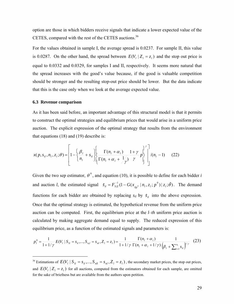
6.3 Revenue comparison

As it has been said before, an important advantage of this structural model is that it permits

to construct the optimal strategies and equilibrium prices that would arise in a uniform price

auction. The explicit expression of the optimal strategy that results from the environment

that equations (18) and (19) describe is:

)1/(1)1(

)(1);,,,( −

⎥⎥⎥

⎦

⎤

⎢⎢⎢

⎣

⎡

⎪⎭

⎪⎬⎫

⎪⎩

⎪⎨⎧

+

++Γ

+Γ

⎭⎬⎫

⎩⎨⎧

+−= lll

llil

l

lllil np

nn

sn

znspx

γ

γγ

γα

αβθ (22)

Given the two sep estimator, 0θ , and equation (10), it is possible to define for each bidder i

and auction l, the estimated signal )ˆ;|);,|(1(ˆ 01| 0 θlllilpZSil zpznxGFs −= − . The demand

functions for each bidder are obtained by replacing sil by ils into the above expression.

Once that the optimal strategy is estimated, the hypothetical revenue from the uniform price

auction can be computed. First, the equilibrium price at the l–th uniform price auction is

calculated by making aggregate demand equal to supply. The reduced expression of this

equilibrium price, as a function of the estimated signals and parameters is:

( ) γβγα

αγγ /1

1

10 1

)/1()(

/111),,...,|(

/111

∑ =+++Γ

+Γ+

====+

=l

l n

i illll

llllnllnillll

snn

zZsSsSVEp (23)

36 Estimations of ),,...,|( 1 llnlnllilll zZsSsSVE === , the secondary market prices, the stop out prices,

and )|( lll zZVE = for all auctions, computed from the estimators obtained for each sample, are omitted for the sake of briefness but are available from the authors upon petition.

30

Then the hypothetical revenue from uniform price auction l is computed as just the product

of the equilibrium price times the amount of bonds auctioned. The total hypothetical

revenue obtained with this process is 80,918.48 billions of pesos, while the revenue

observed in the discriminatory auction is 79,767.05 billions of pesos. Hence, had the

Federal Government used the uniform price mechanism to auction its securities instead of

the discriminatory price mechanism, it would have raised 1,151.42 billions of pesos more;

that is, 1.44 percent higher revenues. This also seems to be the case when only the auctions

of sample II are considered. In the sample II auctions the revenue of the uniform price

mechanism is 31,294.72 billions of pesos, which exceeds that one from the discriminatory

price mechanism by 731.69 billions of pesos, a difference of 2.09 percent.

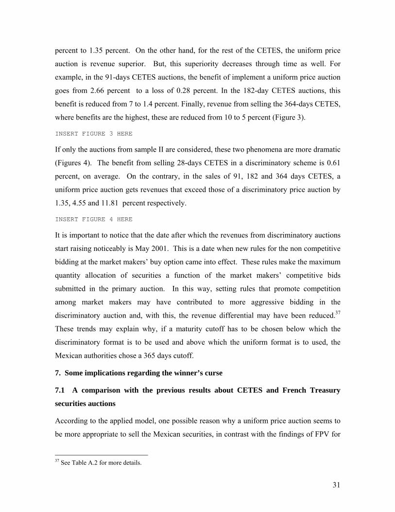
In order to test the significance of these estimates, we calculate the bootstrapped confidence

intervals of the difference in revenue per auction. For the Sample I, we find a significant

difference between the discriminatory and the uniform auction. The bootstrapped mean of

the difference is approximately 6 millions of pesos, with an upper bound of 4.50 million

and a lower bound of 4 million. This difference is higher in Sample II, where we calculate a

bootstrapped mean of 9.61 millions of pesos. This difference shows a confidence interval

of 95% between 12.53 and 5.25 millions of pesos, per auction.

INSERT TABLE 13 HERE

We calculated the bootstrapped interval several times and found that their figures do not

change across calculations. The bootstrap methodology here was not applied through the

whole estimation process since we also estimated the standard errors of the structural

estimators and they are significant. The aggregated difference seems small, but it is

considerably negative in each auction. The estimated density functions for the revenue

difference are shown in Graphs 1 and 2.

INSERT FIGURES 1 AND 2 HERE

It is important to point out two other features of the results. First, that this revenue

superiority from the uniform scheme is reduced throughout the analysis period. Second,

that this revenue superiority is different across CETES with different maturity. For the 28-

day CETES auction, the discriminatory scheme obtains higher revenues than the uniform

one. Benefits derived from the discriminatory auction increase through time, from 0.3

31

percent to 1.35 percent. On the other hand, for the rest of the CETES, the uniform price

auction is revenue superior. But, this superiority decreases through time as well. For

example, in the 91-days CETES auctions, the benefit of implement a uniform price auction

goes from 2.66 percent to a loss of 0.28 percent. In the 182-day CETES auctions, this

benefit is reduced from 7 to 1.4 percent. Finally, revenue from selling the 364-days CETES,

where benefits are the highest, these are reduced from 10 to 5 percent (Figure 3).

INSERT FIGURE 3 HERE

If only the auctions from sample II are considered, these two phenomena are more dramatic

(Figures 4). The benefit from selling 28-days CETES in a discriminatory scheme is 0.61

percent, on average. On the contrary, in the sales of 91, 182 and 364 days CETES, a

uniform price auction gets revenues that exceed those of a discriminatory price auction by

1.35, 4.55 and 11.81 percent respectively.

INSERT FIGURE 4 HERE

It is important to notice that the date after which the revenues from discriminatory auctions

start raising noticeably is May 2001. This is a date when new rules for the non competitive

bidding at the market makers’ buy option came into effect. These rules make the maximum

quantity allocation of securities a function of the market makers’ competitive bids

submitted in the primary auction. In this way, setting rules that promote competition

among market makers may have contributed to more aggressive bidding in the

discriminatory auction and, with this, the revenue differential may have been reduced.37

These trends may explain why, if a maturity cutoff has to be chosen below which the

discriminatory format is to be used and above which the uniform format is to used, the

Mexican authorities chose a 365 days cutoff.

7. Some implications regarding the winner’s curse

7.1 A comparison with the previous results about CETES and French Treasury

securities auctions

According to the applied model, one possible reason why a uniform price auction seems to

be more appropriate to sell the Mexican securities, in contrast with the findings of FPV for

37 See Table A.2 for more details.

32

French securities, is that the conditional variance of the value obtained in this exercise is

considerably higher than the one they get. This can be interpreted as a higher degree of

uncertainty in the good’s value, which would be a reason for the winner’s curse being

stronger in Mexico than in France. In this sense, the values of lα and lβ evaluated at the

sample mean of z can be seen in Table 14. It is important to remember that in this case γlV

follows a gamma distribution with parameters lα and lβ .

INSERT TABLE 14 HERE

According to the Table’s 14 data, the distribution of γlV in our two samples exhibit a

higher variance than the one obtained in FPV. This higher dispersion can be appreciated

better by looking at the coefficients of variation, which also are higher in the Mexican

samples than in the French sample. Therefore, it can be said that the Mexican market

shows more value uncertainty than the French market.

Let us now compare our findings with the previous ones for the CETES with 28 days

maturity date. We construct the variance of the daily funding rate with government

securities over the five-day period leading to and including the day of auction execution -

that is, the variable used to proxy resale risk and information dispersion in the previous

studies- for the periods examined by Umlauf (1993), Laviada et al (1997), as well as in the

present study. For the first two, we construct the revenue of the discriminatory format as

the product of the amount issued times the average allocation price. Similarly, we construct

the revenue of the hypothetical uniform auction as the amount issued times the sum of the

average allocation price plus the mark-up per bid in the uniform auction with respect to the

discriminatory format reported by those authors (which in both cases is positive). Then the

gain of using the uniform format is calculated as the revenue difference between these two

figures. In Table 15.1 we can see that there is a positive relationship between the gains of

using the uniform format instead of the discriminatory one and market uncertainty. While

this gain is positive in the auctions examined by Umlauf and Laviada et al, it is negative in

those we examined. In turn, this is connected with higher market volatility in those

samples than in ours.

INSERT TABLE 15.1 HERE

33

Next let us look for the pattern described above in our results for CETES with different

maturity date. For this exercise, we construct the variance of resale price with the data of

the CETES secondary market price index published by Enlaces Prebon (IEP index), which

is one of the interdealer brokerage firms operating in the Mexican Stock Market.38 This

substitution is necessary because for this exercise we need different resale price volatility

across CETES maturities, which cannot generated from either the daily funding rate or the

weekly price vector of Banco de México used before.39 On the other hand, to consider

comparable samples we only look at 17 auctions of each maturity date (recall that the 364

days CETES are auction monthly, restricting the sample size for the other securities). In

Table 15.2 we can appreciate the same positive relationship between the gains of using the

uniform auction format and market volatility in the CETES with maturity of 28 , 91 and

182 days. But it fails in the case of the 364 days CETES. We think that this obeys to a

problem with the IEP index, due to lower transaction volumes for longer maturities, rather

than to this securities’ resale market being in fact less uncertain than those for the shorter

term maturities.

INSERT TABLE 15.2 HERE

7.2 A simulation exercise with noisier value signals

In this section, we test the conjecture about the magnitude of winner’s curse effect. First,

we generate a more volatile series of the secondary market price. Then we carry out again

the structural econometric procedures of section 6 to obtain the model’s parameters, but

using this new price series for the estimation of the distribution of signals in stage 1 instead

of the original one.

To generate this new series of the secondary market price, we model the observed

secondary market price with an AR (1) process -conditional on the CETES maturity- plus

38 The IEP index for CETES corresponds to the mean market interest rate at 12:15, determined through a survey to 12 participating institutions (Current sources for the CETES’ IEP are Banamex, Bank of America, Banorte, BBV, Bital, Chase Manhattan, Citibank, ING, Invex, JP Morgan, Santander Mexicano and Serfin). The three highest and three lowest reported rates are eliminated, so the CETES average rate is constructed from the remaining six reports. The index is constructed for CETES with 28, 91, 182, and 364 days maturity since June of 1996. 39 However, the IEP indexes have a drawback: they are perception indexes, not executable indexes. This means that there is no intention to buy or sell securities at the quoted rates. This may be a disadvantage for this exercise’s purpose, even though Enlaces Prebon explains that for these perception quotes are better than buy and sell quotes, because the latter tend to be biased by the traders’ market positions at the time of survey.

34

i.i.d. shocks. This model yields a variance of shocks equal to 2.55 and an autoregressive

parameter ρ=0.091. Next, we use the AR (1) approximation method proposed by Tauchen

(1986) to simulate 180 new data of the secondary market price, assuming that the new

series will have the variance observed between June 1995 and March 1997, which is the

period analyzed by Laviada et al (1997). According to the data reported in table 15.1, in

that period the variance of the daily funding rate (their secondary market price variable)

equals 3.49. Therefore, this variance is 55 percent higher than the one that characterizes the

price series in our data set. But this can still be regarded as a conservative simulation.

The parameters estimated with the simulated price data are shown in Table 16. We can

observe a higher estimated value of the parameter γ. This result can be interpreted as

consistent with a setting in which the bidders face less informative signals. In effect, as the

value of γ increases γV becomes smaller (recall that 0<V<1) and the distribution of signals,

[ ]γθ lllZVS svzvsF −−= exp1);,|( 2,| collapses. Also, as the value of gamma increases we

would expect that the uniform price auction produces higher revenues, as a conclusive

effect of the winner’s curse. This is precisely what we find: the new total hypothetical

revenue obtained from the uniform auction now is 81,506.33 billions of pesos. This figure

not only is 2.1 percent higher than the revenue observed from the discriminatory auctions,

but also exceeds by 0.7 percent the revenue obtained in section 6.

INSERT TABLE 16 HERE

8. Conclusions

The share auction framework that supports the structural estimation method of FPV seems

to provide an adequate characterization of Mexico’s CETES auctions during the analysis

period, despite their institutional complexities. The reason is that the buy option allocations

have been a small proportion of the total amount issued by the Mexican Treasury through

the primary auctions. In this sense, the asymmetry that market makers’ buy option may be

inducing in the primary auction behavior did not reflect as substantial changes in the

estimated parameters. With more detailed information regarding the auction and buy

option results it would be desirable to solve for the complete set of equilibrium responses of

the sales mechanism model. But in Mexico, as in many countries, such additional detail is

35

not public data. With the appropriate data, we think it would also be desirable to analyze a

framework with asymmetric bidders, most likely by using numerical solution methods.40

This would probably mimic better some of the characteristics of the data per bidder and bid

reported in section 4.

Although the obtained coefficients are significant and have a plausible size, the estimated

value of the securities does not seem to be too sensitive to changes in the auction

characteristics. Moreover, the sign of some of the coefficients are not very intuitive and

differ across the analyzed samples. While some small sample bias may explain these

findings, a selection criteria that permits choosing the exogenous variables that can best

describe the auction heterogeneity may be needed. The latter would contribute to raise the

power of the estimation procedure and extend its applicability to other securities for which

there is less data available than for the zero coupon bonds, particularly regarding the

secondary market prices.

Our results indicate that the uniform price auction produces higher revenue than the

discriminatory price auction in the analyzed period, given the estimated parameters. In the

study of CETES auctions this is not a new result. Previous estimations with reduced form

equations have produced in the same conclusion. However, we do find evidence that

suggests that market volatility has diminished across the analyzed episodes, suggesting that

the winner’s curse may have been alleviated. As a result, the revenue difference between

auction formats is lower in this study than in Umlauf’s or Laviada´s. However, we find

something new: we detect that the revenue difference between the two auction formats

varies across CETES with different maturity. The discriminatory format produces higher

revenue than the uniform format in the 28 days securities auctions, while the uniform

format produces higher revenue than the discriminatory format in the 91, 182, and 364 days

securities auctions. This positive relation between the gains of the uniform format and the

securities’ maturity coincides with the Mexican Treasury practice of selling securities with

maturity longer than one year through the uniform auction format.

40 See Armantier and Sabih (2003) or Hortacsu (2002) for recent contributions in this area.

36

8. Appendix INSERT TABLES A.1 AND A.2

9. Bibliography

1. Armantier, O. and E. Sabih (2003), “Estimation and Comparison of Treasury Auction

Formats when Bidders are Asymmetric,” mimeograph, State University of New York at

Stony Brook and GREMAQ, Université de Toulouse, May 2003.

2. Bartolini, Leonardo and Carlo Cottarelli (1994), “Treasury Bill Auctions: Issues and

Uses,” IMF Working Paper 94/135.

3. Breedon, F. and J. Ganley (1996), “Bidding and Information: Evidence from Gilt-

Edged Auctions,” Bank of England, Working Paper Series No. 42, January 1996.

4. Février, P., Préget, R., and M. Visser (2002), “Econometrics of Share Auctions,”

CREST Working Paper n° 2002-09, in revision for Econometrica.

5. Fudenberg, D. and J. Tirole (1992), Game Theory, second printing, The MIT Press.

6. Gordy, M. B. (1996), “Hedging Winner’s Curse with Multiple Bids: Evidence from the

Portuguese Treasury Bill Auction,” Bank of Portugal, Research And Statistics

Department WP 21-96, Dec. 1996.

7. Green, W. H. (1993), Econometric Analysis, first edition, Macmillan Publishing

Company.

8. Hamilton, J. D. (1994), Time Series Analysis, first edition, Princeton University Press.

9. Hausman, J. A. and W. K. Newey (1995), “Nonparametric Estimation of Exact

Consumers Surplus and Deadweight Loss,” Econometrica, Vol. 63, Issue 6, Nov. 1995,

1445-1476.

37

10. Hortacsu, A. (2002), “Mechanism Choice and Strategic Bidding in Divisible Good

Auctions: An Empirical Analysis of the Turkish Treasury Auction Market,” mimeo.,

University of Chicago.

11. Hortacsu, A. (2002a), “Bidding Behavior in Divisible Good Auctions: Theory and

Evidence from the Turkish Treasury Auction Market,” mimeo., University of Chicago.

12. Joint Report on the Government Securities Market, Department of the Treasury,

Securities and Exchange Commission, and Board of Governors of the Federal Reserve

System, United States of America, January 1992.

13. Laviada, B. and F. Laviada (1997), Análisis del Mecanismo de Subastas de Valores

Gubernamentales en México, Tesis de Licenciatura en Economia, Universidad

Iberoamericana.

14. Mazón, C. and S. Núñez (1999), “On the optimality of treasury bond auctions: the

Spanish case,” Bank of Spain, Research Document No. 9905.

15. Newey, W. K. and D. L. McFadden (1994), “Large sample estimation and hypothesis

testing,” in R. F. Engle and D. L. McFadden, eds., Handbook of Econometrics, Vol. 4,

2113-2245.

16. Pagan, A. and A. Ullah (1999), Nonparametric Econometrics, first edition, Cambridge

University Press.

17. Pakes, A. (1991), “Dynamic Structural Models: Problems and Prospects. Mixed

Continuous Discrete Controls and Market Interactions,” Cowles Foundation Discussion

Papers 984, Cowles Foundation, Yale University.

18. Pakes, A. (2003), “Common Sense and Simplicity in Empirical Industrial

Organization,” mimeo., Harvard University.

19. Scalia, A. (1998), “Bidder Profitability under Uniform Price Auctions and Systematic

Reopenings,” Journal of Fixed Income, 47-61.

38

20. Tauchen, G. (1986), “Finite State Markov Chain Approximations” Economic Letters,

20, 17-181.

21. Umlauf, S. R. (1993), “An empirical study of the Mexican Treasury bill auction,”

Journal of Financial Economics, 33, 313-340.

22. Uniform Price Auctions: Evaluation of the Treasury Experience, Department of the

Treasury, U.S. Treasury, October 1995.

23. Uniform Price Auctions: Update of the Treasury Experience, Department of the

Treasury, U.S. Treasury, October 1998.

24. Wilson, R. (1979), “Auctions of Shares,” The Quarterly Journal of Economics, Vol.

93, Issue 4, Nov. 1979, 675-689.

39

Tables and Figures

Table 1. CETES (balance outstanding)

Year CETES Change % Dollar Change% % of All Government Securities1

Pesos Dollars Pesos Dollars

1997 137,812,544 17,081,165 0.51 0.51 1998 127,600,335 12,893,742 -7.41 -24.51 0.36 0.36 1999 129,044,534 13,585,637 1.13 5.37 0.24 0.24 2000 175,068,861 18,217,742 35.67 34.10 0.24 0.24 2001 196,673,885 21,448,703 12.34 17.74 0.26 0.26 2002 197,438,671 18,913,018 0.39 -11.82 0.23 0.23 Source: Banco de México

Table 2. Government Securities; Balance Outstanding 1997-2002

Security Cetes Bondes Udibonos Fixed Rate

Bonds Other

Securities

Total Government Securities1

1997 Pesos 137,812,544 81,768,269 36,678,360 N/E 15,950,568 272,209,741

Dollars 17,081,165 10,134,761 4,546,096 N/E 1,976,992 33,739,014

1998 Pesos 127,600,335 151,835,597 62,833,444 N/E 10,970,484 353,239,859

Dollars 12,893,742 15,342,663 6,349,185 N/E 1108543.98 35,694,134

1999 Pesos 129,044,534 337,270,992 80,008,050 N/E 564 546,324,140

Dollars 13,585,637 35,507,442 8,423,141 N/E 59.3771714 57,516,280

2000 Pesos 175,068,861 420,255,890 86,644,593 34,870,116 0 716,839,460

Dollars 18,217,742 43,732,012 9,016,274 3,628,600 0 74,594,628

2001 Pesos 196,673,885 348,988,019 94,846,730 122,329,819 0 762,838,454

Dollars 21,448,703 38,059,656 10,343,719 13,340,948 0 83,193,026

2002 Pesos 197,438,671 343,345,208 99,767,654 235,088,796 0 875,640,329

Dollars 18,913,018 32,889,677 9,556,930 22,519,594 0 83,879,219 Source: Banco de México

(1) Does not include Bonos de Regulación Monetaria, Bonos IPAB and Federal Government Bonds in foreign currency. Thousand pesos and thousand dollars.

Table 3. Overall information about the CETES auctions

(January 2001-April 2002) Number of Auctions 180 28 days CETES 65 (36.11%) 91 days CETES 65 (36.11%) 182 days CETES 33 (18.33%) 364 days CETES 17 (9.45%) Number of bidders 3,581 Number of bids 13,393 Allocated totally or partially 4,506 (33.64%) Not allocated 8,887 (66.36%) Total amount issued by the Treasury1 879,249,141 Competitive bids in the primary auction 823,388,150 (93.65%) Non competitive bids in the buy option for market makers 55,860,991 (6.35%) (1) Thousands of pesos

40

Table 4. Summary statistics per CETES auction (January 2001-April 2002)

All CETES Variable

Statistic

Number of bidders

Number of bids Amount issued by the Treasury1

Secondary market price

Nominal yield2 Maturity of the security

Cover

Mean 19.46 73.92 4,538,043.48 96.84 10.30 109.18 3.24 Standard Deviation 6.13 19.59 674,815.08 3.14 3.48 94.22 0.90 Max 91 145 5,200,000 100 18.38 364 7.31 Min 12 35 3,300,000 84.81 5.26 27 1.68 Obs 180 180 180 180 180 180 180

28 days CETES Variable

Statistic

Number of bidders

Number of bids Amount issued by the Treasury1

Secondary market price

Nominal yield2 Maturity of the security

Cover

Mean 18.90 72.12 4,500,000.00 99.30 9.13 28.00 3.02 Standard Deviation 2.70 16.54 0.00 0.25 3.07 0.28 0.81 Max 27.00 107.00 4,500,000.00 100.00 16.61 29.00 5.66 Min 15.00 42.00 4,500,000.00 98.74 5.65 27.00 1.70 Obs 65 65 65 65 65 65 65

91 days CETES Variable

Statistic

Number of bidders

Number of bids Amount issued by the Treasury1

Secondary market price

Nominal yield2 Maturity of the security

Cover

Mean 19.63 78.71 5,200,000.00 97.62 9.74 91.00 3.60 Standard Deviation 3.41 18.68 0.00 0.78 2.93 0.28 0.87 Max 29.00 128.00 5,200,000.00 100.00 17.01 92.00 6.37 Min 13.00 35.00 5,200,000.00 95.80 5.92 90.00 2.32 Obs 65 65 65 65 65 65 65

182 days CETES Variable

Statistic

Number of bidders

Number of bids Amount issued by the Treasury1

Secondary market price

Nominal yield2 Maturity of the security

Cover

Mean 18.61 68.86 3,300,000.00 94.91 10.59 178.96 3.38 Standard Deviation 3.11 20.39 0.00 1.41 2.75 5.83 1.17 Max 25.00 112.00 3,300,000.00 97.51 16.53 182.00 7.31 Min 13.00 40.00 3,300,000.00 92.11 6.49 168.00 1.78 Obs 33 33 33 33 33 33 33

364 days CETES Variable

Statistic

Number of bidders

Number of bids Amount issued by the Treasury1

Secondary market price

Nominal yield2 Maturity of the security

Cover

Mean 19.00 78.00 4,646,153.85 89.16 11.20 348.77 3.02 Standard Deviation 3.34 27.70 161,324.64 2.12 2.18 14.52 0.97 Max 25.00 145.00 5,000,000.00 92.23 15.36 364.00 4.45 Min 14.00 43.00 4,500,000.00 85.61 8.34 335.00 1.68 Obs 17 17 17 17 17 17 17

(1) Thousands of pesos (2) Weighted allocation rate of the primary auction.

Table 5. Summary Statistics per bidder or per bid in the CETES auctions

(January 2001-April 2002) Statistic

Variable Mean Standard

Deviation Maximum Minimum Observations

Number of bids per bidder 3.85 0.75 7.69 0.64 3,581 Demanded quantity per bidder1 770,628.39 215,108.12 1,461,470.59 205,625.27 3,581 Demanded quantity per bid1 204,299.71 61,087.98 418,285.71 116,342.35 13,393 Allocated bids per winning bidder 2.04 0.82 4.09 0.12 4,506 Allocated quantity per winning bidder1 576,621.62 531,294.24 2,600,000.00 183,333.33 4,506 Allocated quantity per winning bid1 432,918.42 571,619.13 2,600,000.00 64,705.88 4,506 Price bid 96.68 3.19 99.57 84.55 13,393 Highest price bid – lowest price bid 0.38 0.42 2.58 0.04 13,393 (1) Thousands of pesos

41

Table 6. Summary Statistics per CETES buy option (January 2001-April 2002)

CETES a 28 días Variable

Statistic

Supply1 Demanded Amount1

Allocated Amount1

Demanded Amount /

Supply (%)

Amount Issued at the Primary

Auction!

Demanded Amount / Amount

Issued at the Primary Auction

(%) Mean 900,000,000.00 471,186,288.14 342,237,135.59 52.35 4,500,000,000.00 10.47 Median 900,000,000.00 200,000,000.00 200,000,000.00 22.22 4,500,000,000.00 4.44 Mode 900,000,000.00 0.00 0.00 0.00 4,500,000,000.00 0.00 Standard Deviation 0.00 614,042,270.30 365,826,041.46 68.23 0.00 13.65 Maximum 900,000,000.00 2,050,000,000.00 900,000,000.00 227.78 4,500,000,000.00 45.56 Minimum 900,000,000.00 0.00 0.00 0.00 4,500,000,000.00 0.00

CETES a 91 días Variable

Statistic

Supply1 Demanded Amount1

Allocated Amount1

Demanded Amount /

Supply (%)

Amount Issued at the Primary

Auction!

Demanded Amount / Amount

Issued at the Primary Auction

(%) Mean 1,040,000,000.00 504,718,305.08 399,983,050.85 48.53 5,196,610,169.49 9.72 Median 1,040,000,000.00 100,000,000.00 100,000,000.00 9.62 5,200,000,000.00 1.92 Mode 1,040,000,000.00 0.00 0.00 0.00 5,200,000,000.00 0.00 Standard Deviation 0.00 666,345,528.35 457,764,262.91 64.07 26,037,782.20 12.82 Maximum 1,040,000,000.00 2,580,000,000.00 1,040,000,000.00 248.08 5,200,000,000.00 49.62 Minimum 1,040,000,000.00 0.00 0.00 0.00 5,000,000,000.00 0.00

CETES a 182 días Variable

Statistic

Supply1 Demanded Amount1

Allocated Amount1

Demanded Amount /

Supply (%)

Amount Issued at the Primary

Auction!

Demanded Amount / Amount

Issued at the Primary Auction

(%) Mean 660,000,000.00 241,333,333.33 222,666,666.67 36.57 3,300,000,000.00 7.31 Median 660,000,000.00 0.00 0.00 0.00 3,300,000,000.00 0.00 Mode 660,000,000.00 0.00 0.00 0.00 3,300,000,000.00 0.00 Standard Deviation 0.00 323,107,042.51 287,113,258.12 48.96 0.00 9.79 Maximum 660,000,000.00 960,000,000.00 660,000,000.00 145.45 3,300,000,000.00 29.09 Minimum 660,000,000.00 0.00 0.00 0.00 3,300,000,000.00 0.00

CETES a 364 días Variable

Statistic

Supply1 Demanded Amount1

Allocated Amount1

Demanded Amount /

Supply (%)

Amount Issued at the Primary

Auction!

Demanded Amount / Amount

Issued at the Primary Auction

(%) Mean 927,142,857.14 402,857,142.86 385,000,000.00 42.71% 4,635,714,285.71 8.54% Median 920,000,000.00 0.00 0.00 0.00% 4,600,000,000.00 0.00% Mode 920,000,000.00 0.00 0.00 0.00% 4,600,000,000.00 0.00% Standard Deviation 31,968,390.98 492,691,642.86 468,233,176.62 52.20% 159,841,954.91 10.44% Maximum 1,000,000,000.00 1,100,000,000.00 1,000,000,000.00 122.22% 5,000,000,000.00 24.44% Minimum 900,000,000.00 0.00 0.00 0.00% 4,500,000,000.00 0.00% (1) Pesos.

Table 7. Frequency distribution of the CETES buy option (January 2001-April 2002)

Maturity 28 days CETES 91 days CETES 182 days CETES 364 days CETES Event Obs % Obs % Obs % Obs % Market makers Aggregated demand is zero

21

36.21

25

43.10

17

58.62

8

61.54

Market makers Aggregated demand is less than supply

25

43.10

22

37.93

10

34.48

4

30.77

Market makers Aggregated Demand exceeds supply

12

20.69

11

18.97

2

6.90

1

7.69

Total

58

100.00

58

100.00

29

100.00

13

100

42

Table 8. Overall information about the CETES auctions of sample II Number of auctions 71 28 days CETES 21 (29.58%) 91 days CETES 25 (35.21%) 182 days CETES 17 (23.94%) 364 days CETES 8 (11.27%) Number of bidders 1,343 Number of bids 5,018 Allocated totally or partially 1,829 (36.45%) Not allocated 3,189 (63.55%) Total amount issued by the Treasuryl1 323,788,150 Competitive bids in the primary auction 323,788,150 (100%) Non competitive bids in the buy option for market makers 0 (1) Thousands of pesos.

Table 9. Summary Statistics per CETES auction of Sample II All CETES

Variable Statistic

Number of bidders

Number of bids

Amount issued by the

Treasury1

Secondary Market

Price

Nominal yield2

Maturity of the security

Cover

Mean 18.92 70.68 4,467,605.63 96.26 10.49 121.92 3.08 Standard Deviation 3.24 20.06 724,228.58 3.56 3.16 97.61 1.05 Max 29.00 128.00 5,200,000.00 100.00 17.01 364.00 7.31 Min 13.00 35.00 3,300,000.00 85.61 6.15 28.00 1.70 Obs 71 71 71 71 71 71 71 (1) Thousands of pesos (2) Weighted allocation rate of the primary auction.

Table 10. Summary Statistics per bidder or bid in the CETES auctions of sample II Statistic

Variable Mean Standard

Deviation Maximum Minimum Observations

Number of bids per bidder 3.70 0.65 5.19 2.47 1,343 Demanded quantity per bidder1 722,790.41 225,440.52 1,457,385.29 372,155.79 1,343 Demanded quantity per bid1 197,314.89 62,019.37 418,285.71 116,342.35 5,018 Allocated bids per winning bidder 2.12 0.82 3.71 0.31 1,829 Allocated quantity per winning bidder1 693,967.89 671,205.67 2,600,000.00 183,333.33 1,829 Allocated quantity per winning bid1 530,135.86 725,451.89 2,600,000.00 73,333.33 1,829 Price bid 96.12 3.57 99.52 85.36 5,018 Highest price bid – lowest price bid 0.41 0.42 2.58 0.05 5,018 (1) Thousands of pesos.

Table 11. Second step estimate of θ in sample I Estimate of alpha: Standard Error Constant -15.27710 0.97630 Secondary market price 148.42810 0.92758 Nominal yield -12.55930 0.11267 Maturity1 -4.74920 0.43610 Estimate of beta: Constant -29.80050 0.63808 Secondary market price 151.14290 0.60659 Nominal yield 12.93690 0.07355 Maturity1 0.38890 0.28267 Gamma 118.73350 0.66655 (1) Divided by 364.

43

Table 12. Second step estimate of θ in sample II

Estimate of alpha: Standard Error Constant 7.15020 2.88818 Secondary market price 105.41850 2.71999 Nominal yield -150.45390 0.34874 Maturity1 -3.57240 1.36952 Estimate of beta: Constant 493.54630 0.31200 Secondary market price -7.68270 0.29487 Nominal yield 24.94770 0.03710 Maturity1 5.82230 0.14142 Gamma 287.84650 1.58210 (1) Divided by 364

Table 13. Mean of difference in revenue –Discriminatory minus estimated uniform

Confidence interval (95%)

Mean Mean bootstrap Lower bound Upper bound

Sample I -6.3968 -7.4383 -8.4476 -4.5051

Sample II -9.0138 -9.6176 -12.5375 -5.2512 In millions of pesos

Table 14. αl, βl, conditional mean, variance and variation coefficient of Vγ1

αl βl Mean (αl/βl)

Variance (αl/βl

2) Variation coefficient

Sample I 125.68 117.97 1.0653 0.0090 0.0891

Sample II 91.65 490.72 0.1868 0.0004 0.1071

Février,Préget, and Visser (2002) 3045.04 848.72 3.5878 0.0042 0.0181 (1) Evaluated at the characteristics’ sample mean.

Table 15.1 Auction Revenue and Market Volatility Comparison with Previous Reduced Form Estimations for 28 days CETES

Analysis Date

Dummy variable of auction format

Observed Revenue of Discriminatory

Auctions (millions of pesos)

Hypothetical Revenue of Uniform

Auctions (millions of pesos)

Revenue Difference

(percentage)

Variance of the daily funding

rate Aug 1986- May1991 (Umlauf, 1993) 2.44pb 73.742 73.742 0.000% 0.160 Jun 1995- Mar 1997 (Laviada et al, 1997) 18.96pb 8,557.539 8,557.706 0.002% 3.498 Jan 2001-Apr 2002 (present) -- 29,657,590.272 29,398,572.997 -0.873% 0.096

Table 15.2 Auction Revenue and Market Volatility Comparison Across Maturities

CETES Maturity

Observed Revenue of Discriminatory

Auctions (millions of pesos)

Hypothetical Revenue of Uniform

Auctions (millions of pesos)

Revenue Difference

(percentage)

Variance of the daily

IEP index

28 days 7,572.253 7,518.962 -0.70% 0.052 91 days 8,564.527 8,690.297 1.47% 0.064 182 days 5,321.119 5,511.703 3.58% 0.067 364 days 7,141.314 7,807.403 9.33% 0.046

44

Table 16 Second step estimate of θ using a simulated secondary market price series distributed with mean 3.70 and variance 3.49

Estimate of alpha: Standard Error Constant 327.1935 0.00000015 Secondary market price 162.8496 0.00001419 Nominal yield 20.2399 0.00000151 Maturity1 447.9777 0.00000002 Estimate of beta: Constant 5.4844 0.00003000 Secondary market price 34.3807 0.00290531 Nominal yield 82.8601 0.00030871 Maturity1 2031.6185 0.00000309 Gamma 745.6563 14.10575237

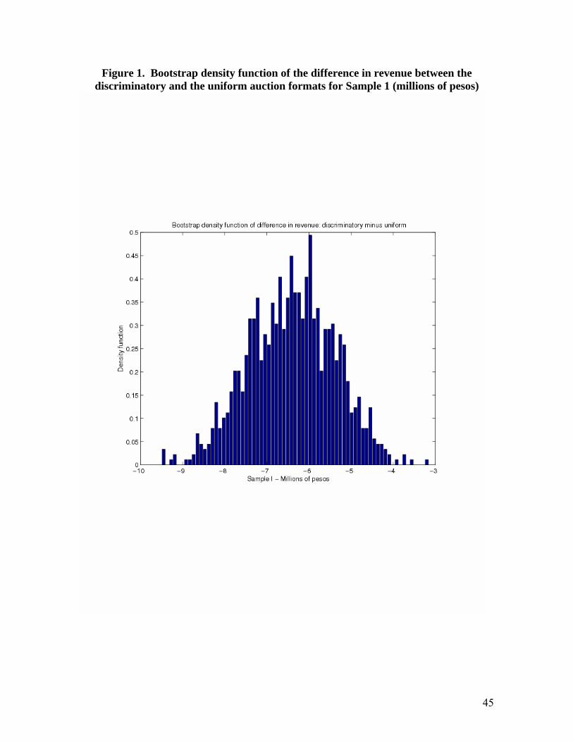
45

Figure 1. Bootstrap density function of the difference in revenue between the discriminatory and the uniform auction formats for Sample 1 (millions of pesos)

46

Figure 1. Bootstrap density function of the difference in revenue between the discriminatory and the uniform auction formats for Sample II (millions of pesos)

47

Figure 3. Revenue difference between the (observed) discriminatory auction and the (hypothetical) uniform auction in Sample I

a. 28 days CETES (percentages)

b. 91 days CETES (percentages)

c. 182 days CETES (percentages)

d. 364 days CETES (percentages)

0.00%

0.20%

0.40%

0.60%

0.80%

1.00%

1.20%

1.40%

1.60%

09/0

1/20

01

09/0

2/20

01

09/0

3/20

01

09/0

4/20

01

09/0

5/20

01

09/0

6/20

01

09/0

7/20

01

09/0

8/20

01

09/0

9/20

01

09/1

0/20

01

09/1

1/20

01

09/1

2/20

01

09/0

1/20

02

09/0

2/20

02

09/0

3/20

02

09/0

4/20

02

-3.50%

-3.00%

-2.50%

-2.00%

-1.50%

-1.00%

-0.50%

0.00%

0.50%

09/0

1/20

01

09/0

2/20

01

09/0

3/20

01

09/0

4/20

01

09/0

5/20

01

09/0

6/20

01

09/0

7/20

01

09/0

8/20

01

09/0

9/20

01

09/1

0/20

01

09/1

1/20

01

09/1

2/20

01

09/0

1/20

02

09/0

2/20

02

09/0

3/20

02

09/0

4/20

02-18.00%

-16.00%

-14.00%

-12.00%

-10.00%

-8.00%

-6.00%

-4.00%

-2.00%

0.00%

09/0

1/20

01

09/0

2/20

01

09/0

3/20

01

09/0

4/20

01

09/0

5/20

01

09/0

6/20

01

09/0

7/20

01

09/0

8/20

01

09/0

9/20

01

09/1

0/20

01

09/1

1/20

01

09/1

2/20

01

09/0

1/20

02

09/0

2/20

02

09/0

3/20

02

09/0

4/20

02

-18.00%

-16.00%

-14.00%

-12.00%

-10.00%

-8.00%

-6.00%

-4.00%

-2.00%

0.00%

23/0

1/20

01

23/0

2/20

01

23/0

3/20

01

23/0

4/20

01

23/0

5/20

01

23/0

6/20

01

23/0

7/20

01

23/0

8/20

01

23/0

9/20

01

23/1

0/20

01

23/1

1/20

01

23/1

2/20

01

23/0

1/20

02

23/0

2/20

02

23/0

3/20

02

48

Figure 4. Revenue difference between the (observed) discriminatory auction and the (hypothetical) uniform auction in Sample II

a. 28 days CETES (percentages)

b. 91 days CETES ( percentages)

c. 182 days CETES ( percentages)

d. 364 days CETES ( percentages)

0.00%

0.10%

0.20%

0.30%

0.40%

0.50%

0.60%

0.70%

0.80%

0.90%

20/0

2/20

01

20/0

3/20

01

20/0

4/20

01

20/0

5/20

01

20/0

6/20

01

20/0

7/20

01

20/0

8/20

01

20/0

9/20

01

20/1

0/20

01

20/1

1/20

01

20/1

2/20

01

20/0

1/20

02

20/0

2/20

02

20/0

3/20

02-3.50%

-3.00%

-2.50%

-2.00%

-1.50%

-1.00%

-0.50%

0.00%

20/0

2/20

01

20/0

3/20

01

20/0

4/20

01

20/0

5/20

01

20/0

6/20

01

20/0

7/20

01

20/0

8/20

01

20/0

9/20

01

20/1

0/20

01

20/1

1/20

01

20/1

2/20

01

20/0

1/20

02

20/0

2/20

02

20/0

3/20

02-8.00%

-7.00%

-6.00%

-5.00%

-4.00%

-3.00%

-2.00%

-1.00%

0.00%

20/0

2/20

01

20/0

3/20

01

20/0

4/20

01

20/0

5/20

01

20/0

6/20

01

20/0

7/20

01

20/0

8/20

01

20/0

9/20

01

20/1

0/20

01

20/1

1/20

01

20/1

2/20

01

20/0

1/20

02

20/0

2/20

02

-16.00%

-14.00%

-12.00%

-10.00%

-8.00%

-6.00%

-4.00%

-2.00%

0.00%

01/0

2/20

01

01/0

3/20

01

01/0

4/20

01

01/0

5/20

01

01/0

6/20

01

01/0

7/20

01

01/0

8/20

01

01/0

9/20

01

01/1

0/20

01

01/1

1/20

01

49

Table A.1. CETES’ Sales Mechanisms (1978-2002) Date Mechanism 1978-1982 Tap with a fixed rate 1982-1985 Discriminatory auction with fixed offered amount

- Limit to the maximum bid per bidder is 40 percent of the amount issued 1985-July 1986 Tap with a fixed rate July 1986-July 1990 Discriminatory auction with variable offered amount.

- Brokerage houses cannot bid for debt of more than a hundred times their capital basis. - In July 1989 the limit to the maximum bid per bidder is raised to 60 percent of the amount issued.

July 1989-January 1993 Uniform auction with variable offered amount

January 1993-April 1994 Discriminatory auction with variable offered amount (allocations to non competitive bids in the primary auction are reduced).

April 1994-November 1995 Uniform auction with variable offered amount November 1995-April 2002 Discriminatory auction with variable offered amount (allocations to non

competitive bids in the primary auction are reduced). - No institution can bid for debt of more than a hundred times their capital basis. - Banks were the only institutions allowed to submit bids in account for others until 2000. - Since January 2000 the Treasury may increase the supply of 182 and 364 days CETES. - “Market makers” mechanism is introduced in October 2000.

Source: Banco de México’s Yearly Report (several numbers) and regulatory dispositions for financial intermediaries.

50

Table A.2. Key Modifications to the Treasury Securities Market Maker Mechanism in Mexico, 2000-2001

Date Modification October 2000

- Those financial institutions willing to become market makers should present a petition within the first 10 market days of the semester before the one they want to start to operate. - The evaluation of the market making activity index will take place every 6 months. The accumulated activity index during the previous 6 months will be used to determine which financial intermediaries may operate as market makers during the next six months. - The maximum spread between bid and ask price quotes in the secondary market is set at 200 basis points. - The weights of the market making activity index are set as: 0.15 for primary market operations, 0.25 for operations in the secondary market with clients, 0.40 for operations in the secondary market among financial intermediaries carried out through trading houses, and 0.20 for operations in the secondary market among financial intermediaries carried out through other means. - The maximum amount of government securities that market makers as a group can get at the weighted allocation rate is set at 20 percent of the amount issued at the primary auction. - The maximum amount of government securities that each market maker can bid for at the weighted allocation rate is set at 20 percent of the amount issued at the primary auction. If market makers’ aggregate demand does not exceed supply, each market maker gets her bid. If market makers’ aggregate demand exceeds supply, bids are served up to the minimum amount between the quantity bid and the supply divided among the number of bidders. The rest is distributed proportionally according to the each market maker’s original quantity bid until supply is exhausted.

January 2001

- The maximum amount of government securities that each market maker can get at the weighted allocation rate is set at the minimum between 20 percent of the amount issued at the primary auction and the amount allocated to her at the primary auction. If market makers’ aggregate demand does not exceed supply, each market maker gets her bid. If market makers’ aggregate demand exceeds supply, bids are served proportionally according to each market maker’s original quantity bid and the percentage allocated to her at the primary auction.

May 2001 The weights of the market making activity index are set as: 0.20 for primary market operations, 0.30 for operations in the secondary market with clients, 0.30 for operations in the secondary market among financial intermediaries carried out through trading houses, and 0.20 for operations in the secondary market among financial intermediaries carried out through other means. - The maximum amount of government securities that each market maker can get at the weighted allocation rate is set at the minimum between 20 percent of the amount issued at the primary auction and the amount of computable bids that she presened at the primary auction. A bid is “computable” if its rate bid is less than or equal to the product of 1.002 times the highest rate that receives an allocation at the primary auction.

November 2001

- Those financial institutions willing to become market makers should present a petition within the first 10 market days of February, May, August, and November. - The evaluation of the market making activity index will take place every month. The activity index will include information of operations carried out by the institutions and ordered in measuring periods that correspond to the last 6 months. - The maximum spread between bid and ask price quotes in the secondary market is set at 125 basis points. - The maximum amount of government securities that each market maker can get at the weighted allocation rate is set at the minimum between 20 percent of the amount issued at the primary auction and the amount of computable bids that she presened at the primary auction. A bid is “computable” if its rate bid is less than or equal to the product of:

a) 1.0035 times the highest rate that receives an allocation at the primary auction, if the market maker’s activity index is the highest one;

b) 1.003 times the highest rate that receives an allocation at the primary auction, if the market maker’s activity index is the second highest one;

c) 1.0025 times the highest rate that receives an allocation at the primary auction, if the market maker’s activity index is the third highest one;

d) 1.002 times the highest rate that receives an allocation at the primary auction, for the other market makers.

Source: Banco de Mexico’s regulatory dispositions for banks and brokerage houses.