Embed Size (px)
Citation preview

arX
iv:1
209.
0794
v1 [
quan
t-ph
] 4
Sep
201
2 OPTIMAL BACON-SHOR CODES
JOHN NAPP and JOHN PRESKILL
Institute for Quantum Information and Matter, California Institute of Technology
Pasadena, CA 91125, USA
We study the performance of Bacon-Shor codes, quantum subsystem codes which are wellsuited for applications to fault-tolerant quantum memory because the error syndromecan be extracted by performing two-qubit measurements. Assuming independent noise,we find the optimal block size in terms of the bit-flip error probability pX and thephase error probability pZ , and determine how the probability of a logical error dependson pX and pZ . We show that a single Bacon-Shor code block, used by itself withoutconcatenation, can provide very effective protection against logical errors if the noise ishighly biased (pZ/pX ≫ 1) and the physical error rate pZ is a few percent or below. Wealso derive an upper bound on the logical error rate for the case where the syndromedata is noisy.
Keywords: Quantum error correction
1 Introduction
Bacon-Shor codes [1, 2] are quantum subsystem codes [3, 4] which are well suited for ap-
plications to fault-tolerant quantum memory [5, 6], because error syndrome information can
be extracted by measuring only two-qubit operators that are spatially local if the qubits are
arranged in a two-dimensional lattice. In this paper we assess the performance of these codes.
We consider noise models such that qubits in the code block are subject to both bit flip
(X) errors and dephasing (Z) errors, where the bit flips occur with probability pX and phase
errors occur with probability pZ . We assume that the noise acts independently on each qubit,
and that the X and Z errors are uncorrelated. Under these assumptions we find the optimal
block size of the code, and the failure probability achieved by this optimal code. We obtain
analytic formulas for the optimal failure probability for the case of unbiased noise (pX = pZ)
and the case of highly biased noise (b ≡ pZ/pX ≫ 1). In both cases the formula applies in
the asymptotic limit of small pZ . Our results show that the failure probability of the optimal
code falls exponentially in 1/pZ . We also consider the case where the code’s syndrome bits
are prone to error, and derive upper bounds on the failure probability in that case.
We find that for the case of unbiased noise (pZ = pX ≡ p), the optimal Bacon-Shor code
1

2 Optimal Bacon-Shor Codes
achieves the failure probability
BSOptimalFailProb(p) =
(
2
π ln 2
)1/2
exp
(
ln2 2
8
)
p1/2 exp
(
− ln2 2
8p+O(p)
)
(1)
or
ln[BSOptimalFailProb(p)] = −A/p− (0.5) ln(1/p) + C +O(p), (2)
where
A = .0600566, C = .0175217. (3)
For the case of highly biased noise, we find
ln[BSOptimalFailProb(pZ, b)] = −A(b)/pZ − (0.5) ln(1/pZ) + C(b) +O(pZ polylog(b)), (4)
where
A(b) =1
8
(
W (√b))2
+O(b−1/2 ln b); (5)
here W denotes the Lambert W function, with asymptotic expansion
W (√b) = ln
√b− ln ln
√b+
ln ln√b
ln√b
+O
(
ln ln√b
ln2√b
)
. (6)
We also compute the asymptotic form of C(b) for b ≫ 1.
In the case where the error syndrome is noisy, the reliability of the syndrome can be
improved by measuring it repeatedly. We consider an idealized noise model such that qubit
errors and syndrome measurement errors are equally likely and independent. For that model
we derive a lower bound on the coefficient A(b) of 1/pZ in the natural logarithm of the logical
failure rate, finding
A(b) ≥ Z(b)
4µ2W
(√
b
4Z(b)
)
, (7)
where µ = 2.63816 is the connective constant of a self-avoiding walk on a two-dimensional
square lattice, and Z(b) is a slowly varying monotonic function which ranges from 1/e to 1
as b increases from 1 to infinity. This bound applies for any value of b ≥ 1.
Previous work [7, 8] on the applications of Bacon-Shor codes to fault-tolerant quantum
computing has focused on relatively small codes used at the bottom layer of a concatenated
coding scheme. Here we emphasize that a sufficiently large Bacon-Shor code, used by itself
without concatenation, can also be quite effective if the physical error rate is low enough. For
example, if the syndrome is perfect, then the probability of a logical failure is below 2×10⁻¹⁹
for pZ = .01, b = 100, and below 10−12 for pZ = .03, b = 1000. Fault-tolerant circuits based
on Bacon-Shor codes will be more fully discussed and analyzed in a separate paper [9], where
we consider in particular the case of highly biased noise.
J. Napp and J. Preskill 3
2 2D Bacon-Shor code
The two-dimensional Bacon-Shor code [1, 2] is a quantum subsystem code (really a family
of codes), which pieces together two dual quantum repetition codes, one protecting against
bit flip errors and one protecting against phase errors. Like any subsystem code [3, 4], it can
be defined by its “gauge algebra” — a set of Pauli operators that commute with the logical
operators. The center of the gauge algebra is the code’s stabilizer group, and the code space
is determined by fixing the eigenvalues of all the stabilizer operators to be (say) +1. Other
operators in the gauge algebra act nontrivially on “gauge qubits” but trivially on the code’s
protected qubits.
Specifically, we consider combining a length-m repetition code to protect against Z errors
with a length-n repetition code to protect against X errors, where Z and X denote the single-
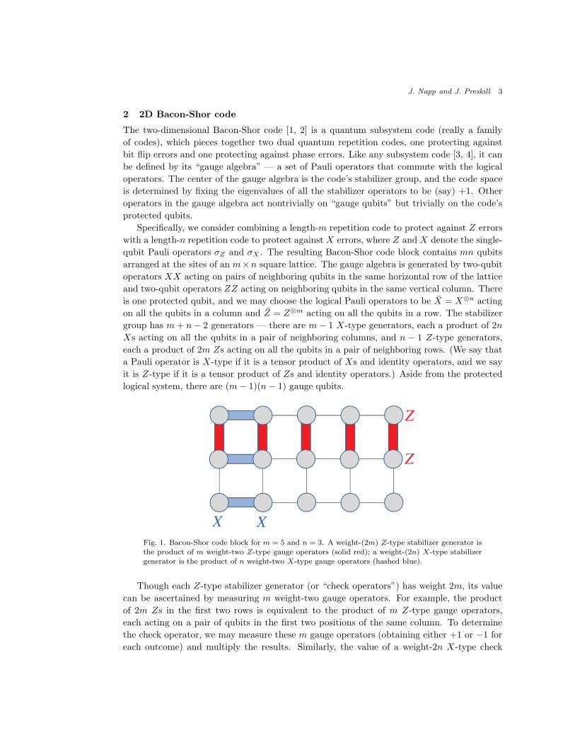
qubit Pauli operators σZ and σX . The resulting Bacon-Shor code block contains mn qubits
arranged at the sites of an m×n square lattice. The gauge algebra is generated by two-qubit
operators XX acting on pairs of neighboring qubits in the same horizontal row of the lattice
and two-qubit operators ZZ acting on neighboring qubits in the same vertical column. There
is one protected qubit, and we may choose the logical Pauli operators to be X = X⊗n acting
on all the qubits in a column and Z = Z⊗m acting on all the qubits in a row. The stabilizer
group has m+ n− 2 generators — there are m− 1 X-type generators, each a product of 2n
Xs acting on all the qubits in a pair of neighboring columns, and n − 1 Z-type generators,
each a product of 2m Zs acting on all the qubits in a pair of neighboring rows. (We say that
a Pauli operator is X-type if it is a tensor product of Xs and identity operators, and we say
it is Z-type if it is a tensor product of Zs and identity operators.) Aside from the protected
logical system, there are (m− 1)(n− 1) gauge qubits.
X X
Z
Z
Fig. 1. Bacon-Shor code block for m = 5 and n = 3. A weight-(2m) Z-type stabilizer generator isthe product of m weight-two Z-type gauge operators (solid red); a weight-(2n) X-type stabilizergenerator is the product of n weight-two X-type gauge operators (hashed blue).
Though each Z-type stabilizer generator (or “check operators”) has weight 2m, its value
can be ascertained by measuring m weight-two gauge operators. For example, the product
of 2m Zs in the first two rows is equivalent to the product of m Z-type gauge operators,
each acting on a pair of qubits in the first two positions of the same column. To determine
the check operator, we may measure these m gauge operators (obtaining either +1 or −1 for
each outcome) and multiply the results. Similarly, the value of a weight-2n X-type check
4 Optimal Bacon-Shor Codes
operator can be found by measuring n weight-two X-type gauge operators and multiplying
the results. Furthermore, since all check operators commute with all gauge-qubit operators,
measuring X-type gauge qubit operators to determine the value of an X-type check operator
does not disturb the values of any Z-type check operators (though it may flip the value of
Z-type gauge operators), and vice-versa.
If m and n are both odd, then the code can correct (m− 1)/2 Z errors and (n− 1)/2 X
errors. To describe the error recovery procedure, it is useful to exploit the freedom to “fix the
gauge”, i.e. apply gauge operators to the block that commute with the logical qubit operators.
An even number of X errors in a row can be “gauged away” by applying gauge operators. If
there are an odd number of X errors in a row, we may “gauge away” all errors except one,
which can be moved into the first position in the row. Thus, in an appropriate gauge, X
errors occur only in the first column. Likewise, in an appropriate gauge, Z errors occur only
in the first row. In this gauge, then, the check operators test whether two neighboring qubits
in the first column agree in the Z basis, and whether two neighboring qubits in the first row
agree in the X basis. Error recovery proceeds by applying X to at most (n− 1)/2 qubits in
the first column, to restore all Z-type check operators to the value +1, and by applying Z to
at most (m− 1)/2 qubits in the first row, to restore all X-type check operators to the value
+1. Thus, error recovery is successful if the number of rows with an odd number of X errors
is at most (n− 1)/2 and if the number of columns with an odd number of Z errors is at most
(m− 1)/2.
If we choose the gauge so that ZZ = +1 for any pair of qubits in the same column, then
the eigenstates of X with eigenvalues ±1 become
|±〉C ∝ (|00 · · · 0〉 ± |11 · · · 1〉)⊗m; (8)
these are tensor products of m length-n “cat states” in the standard basis, one for each
column. If we choose the gauge so that XX = +1 for any pair of qubits in the same row,
then the eigenstates of Z with eigenvalues ±1 becomes
|0〉C ∝ (|++ · · ·+〉+ | − − · · ·−〉)⊗n,
|1〉C ∝ (|++ · · ·+〉 − | − − · · ·−〉)⊗n; (9)
these are tensor products of n length-m “cat states” in the dual basis, one for each row.
To perform a destructive measurement of the logical operator Z, we can measure all mn
qubits in the Z basis, compute the parity of the outcomes for each row, and then decode
the measurement by performing a majority vote on the row parities. Likewise, to perform a
destructive measurement of the logical operator X, we can measure all mn qubits in the X
basis, compute the parity of the outcomes for each column, and then decode the measurement
by performing a majority vote on the column parities.
3 Failure probability for the 2D Bacon-Shor code
Consider an independent noise model in which the probability of an X error for each qubit
is pX , and the probability of a Z error is pZ (that is, for each qubit, there is no error with
probability (1−pX)(1−pZ), anX error with probability pX(1−pZ), a Z error with probability
(1−pX)pZ and an iY = ZX error with probability pXpZ). For any fixed values of pX and pZ ,

J. Napp and J. Preskill 5
there is an optimal choice for the code dimensions m and n which minimizes the probability of
a logical error. We will estimate the optimal failure probability in the limit of small p. Since
X and Z error recovery are identical (except for the interchange of the rows and columns of
the lattice), we will estimate the probability of a logical Z error; the same derivation also
applies to the probability of a logical X error.
First we note that for a column of length n, if Z errors occur independently with probability
p at each position, then the probability of an odd number of errors in the column is
OddProb(p, n) =1
2(1− (1− 2p)n) . (10)
We derive this formula by observing that the terms of even order in p in the binomial expan-
sions of ((1− p) + p) and ((1− p)− p) are identical, while the terms of odd order in p are the
same except for a sign flip; hence the difference 12 (1− (1− 2p)n) sums up all the odd-order
terms. To minimize the probability of a logical error for given p, we will choose n and m so
that p2mn is O(1). Therefore in the limit of large n we may use the approximation
OddProb(p, n) =1
2
(
1− exp[
−2p(1 + p)n+O(p3n)])
. (11)
We keep track of the O(p2n) in the exponential because OddProb(p, n) will be raised to a
power O(m) in the expression for the Bacon-Shor failure probability.
Now consider a length-m repetition code, where bit errors occur independently with prob-
ability x. If m is odd, an encoded error occurs if the number of bit errors is (m + 1)/2 or
more. Therefore the failure probability of the repetition code is
RepFailProb(x,m) =
m∑
k=(m+1)/2
(
m
k
)
xk(1− x)m−k
=
(
x
1− x
)1/2
[x(1 − x)]m/2
(m−1)/2∑
r=0
(
mm+12 + r
)(
x
1− x
)r
. (12)
From the Stirling approximation,
(
mm+12 + r
)
≈ 2m(
2
πm
)1/2
exp
(
− 2
m
(
r +1
2
)2)
, (13)
neglecting a multiplicative O(1/m) correction. Making another O(1/m) multiplicative error,
we may replace the exponential inside the sum over r by 1, obtaining
RepFailProb(x,m) ≈ 2m(
2
πm
)1/2(x
1− x
)1/2
[x(1 − x)]m/2
(m−1)/2∑
r=0
(
x
1− x
)r
, (14)
and we also make a negligible error by extending the upper limit on the sum to infinity, finding
∞∑
r=0
(
x
1− x
)r
=1− x
1− 2x, (15)

6 Optimal Bacon-Shor Codes
and thus
RepFailProb(x,m) ≈(
2
πm
)1/2(x(1 − x)
(1 − 2x)2
)1/2
[4x(1− x)]m/2
. (16)
To compute the probability of a Z-type logical error for the Bacon-Shor code, we substitute
OddProb(p, n) for x in the expression for RepFailProb(x,m), finding
[4x(1− x)]m/2 ≈(
1− exp[
−4p(1 + p)n+O(p3n)])m/2
= exp
(
2p2mn[1 +O(p) +O(p2n)]
e4pn − 1
)
(
1− e−4pn)m/2
, (17)
and
x(1 − x)
(1 − 2x)2≈ 1
4
(
e4pn − 1)
; (18)
hence
BSZFailProb(pZ,m, n) = RepFailProb(OddProb(pZ , n),m)
≈ 1√2πm
exp
[
2p2Zmn
e4pZn − 1
]
(
e4pZn − 1)1/2 (
1− e−4pZn)m/2
,
(19)
up to multiplicative corrections higher order in pZ (assuming pZn and pZm are O(1)). By
the same argument, the probability of an X-type logical error is given by a similar expression,
but with m and n interchanged and pZ replaced by pX :
BSXFailProb(pX ,m, n) = RepFailProb(OddProb(pX ,m), n)
≈ 1√2πn
exp
[
2p2Xmn
e4pXm − 1
]
(
e4pXm − 1)1/2 (
1− e−4pXm)n/2
,
(20)
up to multiplicative corrections higher order in pX (assuming pXm and pXn are O(1)).
3.1 Unbiased noise
If the noise is unbiased (pX = pZ ≡ p), then the optimal Bacon-Shor code is symmetric
(m = n), and the X-type and Z-type logical errors occur with equal probability. To find the
optimal value of n for small p, we note that
ln [BSFailProb(p, n)] ≈ n
2ln(
1− e−4pn)
+ · · · , (21)
where the ellipsis indicates corrections suppressed by powers of p or 1/n. This expression,
regarded as a function of n, attains its minimum when y = pn satisfies
ln(
1− e−4y)
+4y
e4y − 1= 0, (22)
or 4y = ln 2. (Though n is actually required to be an odd integer, we may ignore this
requirement if p is small and n is correspondingly large.) Substituting 4pn ≈ ln 2 into the
J. Napp and J. Preskill 7
expression for the Bacon-Shor failure probability Eq.(19) we find
BSOptimalFailProb(p) ≈(
2
π ln 2
)1/2
exp
(
ln2 2
8
)
p1/2 exp
(
− ln2 2
8p
)
= (1.01768)√p exp
(
− .0600566
p
)
, (23)
or
ln[BSOptimalFailProb(p)] ≈ −A/p+B ln p+ C +O(p) (24)
where
A = .0600566, B = .5, C = .0175217. (25)
This optimal failure probability is achieved by choosing the linear size n of the code such that
pn =1
4ln 2 = .173287. (26)
In terms of the asymptotically optimal linear size n = ln 24p , the optimal failure probability can
be expressed as
BSOptimalFailProb(n) ≈(
2
π ln 2
)1/2
exp
(
ln2 2
8
)(
ln 2
4n
)1/2
exp
(
−n ln 2
2
)
=2ln 2/8
√2πn
2−n/2. (27)
Although there is strictly speaking no accuracy threshold for this family of codes, the
performance of the optimal code is very good when the error rate is sufficiently small. For
example, for p = .001, the optimal value of n is 173, and the corresponding failure probability
is 2.638× 10⁻²⁸, while the asymptotic formula Eq.(23) predicts 2.663× 10⁻²⁸.
3.2 Highly biased noise
If the noise is highly biased (b ≡ pZ/pX ≫ 1), then the optimal Bacon-Shor code is highly
asymmetric — it combines a length-m repetition code to protect against Z errors with a
length-n repetition code to protect against X errors, where m ≫ n. In the limit of large noise
bias, we can find analytic formulas for the optimal values ofm and n and for the corresponding
optimal probability of a logical error.
From Eq.(19) and Eq.(20), we have
ln [BSZFailProb(pZ,m, n)] ≈ m
2ln(
1− e−4pZn)
+ · · · ,
ln [BSXFailProb(pX ,m, n)] ≈ n
2ln(
1− e−4pXm)
+ · · · . (28)
where the ellipsis indicates corrections suppressed by powers of pZ , pX , m−1, n−1. For
b ≡ pZ/pX ≫ 1, the optimal values of m and n are such that 4pXm and e−4pZn are both

8 Optimal Bacon-Shor Codes
small; hence we can justify keeping the leading terms in a power series expansion in these
small quantities, obtaining
ln [BSZFailProb(pZ,m, n)] ≈ −m
2exp (−4pZn)−
m
4exp (−8pZn) + · · · ,
ln [BSXFailProb(pX ,m, n)] ≈ n
2ln (4pXm)− pXmn+ · · · . (29)
For now we neglect the non-leading terms in the expansion of both logarithms, which we will
verify a posteriori are additive corrections of order b−1/2 ln b.
We will minimize the failure probability subject to the constraint that (the leading contri-
butions to) the logs of the Z and X failure probabilities are equal. Because we are neglecting
the higher order terms in both Eq.(28) and Eq.(29), the solution we find many not be the true
optimum, but we will see that it provides an upper bound on the optimal failure probability
which is reasonably tight provided pZ ln4 b and b−1/2 ln b are small. Defining the variables
X = 4pXm, Z = 4pZn, (30)
we want to find the values of X and Z that minimize the function
F (X,Z) = Z lnX (31)
(the log of the failure probability multiplied by 8pZ = 8bpX) subject to the constraint
Z lnX = −bXe−Z. (32)
Introducing a Lagrange multiplier λ to do the constrained minimization, we obtain the equa-
tions
− (λ− 1)Z = λbXe−Z = (λ− 1) lnX (33)
together with the constraint equation Eq.(32); these equations imply
X = e−Z and ZeZ =√b ⇒ X = Z/
√b. (34)
Evaluating F at its minimum yields
Fmin = −Z2. (35)
The solution to the equation ZeZ =√b is the Lambert W function Z = W (
√b), which
has the asymptotic expansion
Z = W (√b) = ln
√b− ln ln
√b+
ln ln√b
ln√b
+O
(
ln ln√b
ln2√b
)
(36)
for b ≫ 1, and the log of the optimal failure probability is
ln [BSZFailProb(pZ ,m, n)] ≈ ln [BSXFailProb(pZ,m, n)] ≈ −W 2(√b)
8pZ+ · · · . (37)

J. Napp and J. Preskill 9
The optimal code has dimensions
n =Z
4pZ≈ 1
4pZW (
√b) ≈ 1
4pZln√b,
m =X
4pX≈ 1
4pZ
√b W (
√b) ≈ 1
4pZ
√b ln
√b, (38)
with aspect ratio m/n =√b. As the bias increases with pZ fixed, the code size creeps up
slowly in the X-protection direction, and more rapidly in the Z-protection direction.
For the optimal code the probability of an odd number of X errors in a row decreases as
b increases according to
OddProb(pX ,m) ≈ 1
2
(
1− e−2pXm)
≈ pXm ≈ 1
4X ≈ 1
4
W (√b)√
b≈ 1
4
ln√b√
b, (39)
while the probability of an odd number of Z errors in a column asymptotically approaches
1/2 according to
OddProb(pZ , n) ≈1
2
(
1− e−2pZn)
=1
2
(
1− e−Z/2)
≈ 1
2
(
1−√X)
, (40)
or
1
2−OddProb(pZ , n) ≈
1
2
(
W (√b)√
b
)1/2
. (41)
The optimal failure probability is much smaller for b ≫ 1 than in the case b = 1 for the same
value of pZ , but the price paid is that the block size is correspondingly significantly larger:
mn =
√b W 2(
√b)
16p2Z, (42)
as compared to
n2 =ln2 2
16p2(43)
in the unbiased case.
Using Eq.(38), we can now evaluate the subleading terms in Eq.(29), finding
− m
4exp (−8pZn) ≈ −m
4X2 ≈ −1
4
(√b W (
√b)
4pZ
)(
W (√b)√
b
)2
= −W 3(√b)
16pZ√b,
−pXmn ≈ −pZb
(√b W (
√b)
4pZ
)(
W (√b)
4pZ
)
= −W 2(√b)
16pZ√b. (44)
Aside from logarithmic factors, these terms are suppressed by O(b−1/2 ln b) compared to the
leading terms in Eq.(29). We therefore expect our estimate for the optimal code dimensions to
be accurate for b ≫ 1. However, although these corrections are small compared to the leading
terms, they are not necessarily negligible, and in particular they can become important as

10 Optimal Bacon-Shor Codes
pZ → 0 with b fixed. To obtain accurate results for small pZ , we should resum the power
series expansion in Eq.(29), or in other words use the full expressions in Eq.(28), with the
appropriate values of m, n, Z, and X plugged in. Thus,
BSZOptimalFailProb(pZ, b) ≈(
1− e−Z)m/2 ≈
(
1− W (√b)√
b
)
√
bW (√
b)8pZ
,
BSXOptimalFailProb(pZ, b) ≈(
1− e−X)n/2 ≈
(
1− exp(
−e−W (√b)))
W (√
b)8pZ , (45)
provide more accurate approximations than exp(
−W 2(√b)/8pZ
)
.
Plugging our solutions for Z and X back into the expressions for the prefactors in Eq.(19)
and Eq.(20), we again find somewhat different scaling with the bias for the two failure prob-
abilities. For the Z failure probability the prefactor is
1√2πm
exp
[
2p2Zmn
e4pZn − 1
]
(
e4pZn − 1)1/2
=
(
2pZn
πZm
)1/2
exp
[ 18Z
2mn
eZ − 1
]
(
eZ − 1)1/2
; (46)
making the approximation eZ − 1 ≈ eZ as before, and using m/n =√b = ZeZ , this becomes
≈(
2pZπ
)1/2
b−1/4Z−1/2eZ3/8eZ/2 =
(
2pZπ
)1/2
Z−1eZ3/8. (47)
For the X failure probability the prefactor is
1√2πn
exp
[
2p2Xmn
e4pXm − 1
]
(
e4pXm − 1)1/2
=
(
2pZπZ
)1/2
exp
[ 18X
2 nm
eX − 1
]
(
eX − 1)1/2
; (48)
making the approximation eX − 1 ≈ X as before, this becomes
≈(
2pZπ
)1/2
Z−1/2 exp
(
X
8√b
)
X1/2 =
(
2pZπ
)1/2
b−1/4 exp
(
X
8√b
)
≈(
2pZπ
)1/2
b−1/4. (49)
We also note that, as in Eq.(17), there are corrections to the factor eZ3/8 of the form
exp
(
1
8Z3 [1 +O(pZ) +O(pZZ)]
)
. (50)
In fact we can sum up these corrections to all orders in pZZ (still neglecting corrections
suppressed by further powers of pZ) to obtain the improved approximation
exp
(
1
8pZ2(
1− e−pZ)
[1 +O(pZ )]
)
. (51)
This correction can be significant for pZ = O(1), but in that case our bound on the failure
probability is rather loose anyway (see below), so including the correction is not so important.

J. Napp and J. Preskill 11
Combining the estimated prefactors with Eq.(45) we obtain the formulas for the failure
probabilities:
BSZOptimalFailProb(pZ, b) ≈(
2pZπ
)1/2
Z−1eZ3/8
(
1− Z√b
)Z
√
b8pZ
,
BSXOptimalFailProb(pZ, b) ≈(
2pZπ
)1/2
b−1/4(
1− exp(
−e−Z))
Z8pZ , (52)
where Z = W (√b). These asymptotic formulas apply if we fix the bias b at a large value and
then allow pZ to become sufficiently small. We see that the nonleading contribution to the
log of the failure probability is approximately 18Z
3 for Z-errors and approximately − 14 ln b for
X errors. These nonleading terms are small compared to the leading term 18pZ
Z2, which we
minimized to obtain our estimates, provided pZZ ≈ pZ ln b ≪ 1. A numerical fit indicates
that the leading correction to our asymptotic formula is approximately (.01)pZ(ln b)δ where
δ ≈ 4. When this correction is small, we expect our estimate of the optimal failure probability
to be reasonably tight.
4 Comparison with numerics
To check the accuracy of our formulas, we have also numerically determined the optimal
values of m and n, and the corresponding optimal failure probability, for a variety of values
of pZ and b.
Fig. 2 shows the numerically optimized failure probability and the asymptotic estimate
Eq.(23) as a function of p ≡ pZ = pX for the unbiased case (b = 1). Our formula overestimates
the exact result by less than 1% for p < .001 and by less than 10% for p < .01.
0.002 0.004 0.006 0.008 0.010p
10- 45
10- 36
10- 27
10- 18
10- 9
BSOptimalFailProb I p M
Fig. 2. The optimal failure probability for the Bacon-Shor code (solid blue curve) and the estimateEq.(23) (dashed red curve) for unbiased noise, as a function of p ≡ pZ = pX . The curves nearlycoincide.
Fig. 3 shows the numerically optimized failure probability and the estimate Eq.(52) as a
function of the bias b for pZ = .01. Here we have actually plotted the total error probability
assuming X and Z errors are independent; that is,
BSOptimalFailProb = BSOptimalZFailProb+BSOptimalXFailProb
−BSOptimalZFailProb×BSOptimalXFailProb. (53)

12 Optimal Bacon-Shor Codes
The agreement is good for b > 10, though the discrepancy grows with increasing b, reaching
about 10% for b = 500.
100 200 300 400 500b
10- 25
10- 20
10- 15
10- 10
10- 5
BSOptimalFailProb I 0.01 , b M
Fig. 3. The optimal failure probability for the Bacon-Shor code (solid blue curve) and the estimateEq.(52) (dashed red curve) for pZ = .01, as a function of the bias b = pZ/pX . The curves nearlycoincide.
Fig. 4 shows the numerically optimized failure probability and the estimate Eq.(52) as
a function of the bias b for pZ = .03. Now our formula badly overestimates the failure
probability for large b, with the discrepancy reaching a factor of 13 for b = 5000. In this
regime, the condition (.01)pZ ln4 b ≪ 1 is not well satisfied ((.01)pZ ln4 b ≈ 1.6 for b = 5000).
1000 2000 3000 4000 5000b
10- 16
10- 13
10- 10
10- 7
10- 4
BSOptimalFailProb I 0.03 , b M
Fig. 4. The optimal failure probability for the Bacon-Shor code (solid blue curve) and the estimateEq.(52) (dashed red curve) for pZ = .03, as a function of the bias b = pZ/pX .
Fig. 5 shows the numerical and analytic results as a function of pZ for b = 1000, and Fig. 6
shows the ratio of the two, illustrating that the agreement improves rapidly as p decreases.

J. Napp and J. Preskill 13
0.02 0.04 0.06 0.08 0.10p z
10- 60
10- 48
10- 36
10- 24
10- 12
BSOptimalFailProb I p z , 1000M
Fig. 5. The optimal failure probability for the Bacon-Shor code (solid blue curve) and the estimateEq.(52) (dashed red curve) for b = 1000, as a function of the error probability pZ .
0.02 0.04 0.06 0.08 0.10p z
1
2
3
4
r I p z , 1000M
Fig. 6. The ratio of the optimal failure probability to the estimate Eq.(52) for b = 1000, as afunction of the error probability pZ . The kinks in the plot occur because the optimal dimensionsm× n of the Bacon-Shor code are integers which change discontinuously.
5 2D Bacon-Shor recovery with syndrome measurement errors
Measurement of the weight-two gauge operator XX can be executed by a simple circuit
with four locations — e.g. preparation of an ancilla qubit in the X = 1 eigenstate |+〉, twosuccessive controlled-X gates with ancilla qubit as control and data qubit as target, followed
by measurement of the ancilla qubit in the X basis. A similar circuit measures ZZ, but with
the controlled-X gates replaced by controlled-Z gates.
A fault in the circuit that flips the ancilla qubit could cause the measurement outcome to
be incorrectly recorded, and a faulty two-qubit gate could damage a qubit in the code block.
However, a single fault in the circuit will not cause two errors in the code block that cannot
be gauged away. A Z-type syndrome bit is obtained by computing the parity of n outcomes
of XX gauge qubit measurements, and an error in any one of those n measurements could flip
the bit, so that the probability of an error in a syndrome bit is roughly n times larger than
the probability of error in each gauge qubit measurement. Similarly, an X-type syndrome bit
is obtained by computing the parity of m outcomes of ZZ gauge qubit measurements, so the
probability of an error in a syndrome bit is roughly m times the probability of error in each
14 Optimal Bacon-Shor Codes
gauge qubit measurement.
Though measurement and data errors may actually be correlated, these considerations
motivate an idealized model for Bacon-Shor error recovery with noisy measurements. For the
Z-type syndrome we consider a repetition code of length m, where both the probability of
error per data bit and the probability of error per syndrome bit is pZ = OddProb(pZ , n),
and pZ is the fixed physical error rate for a Z-type error. Likewise, for the X-type syndrome
we consider a repetition code of length n, where both the probability of error per data bit
and the probability of error per syndrome bit is pX = OddProb(pX ,m), and pX is the fixed
physical error rate for an X-type error.
We will study this model for both unbiased noise and highly biased noise with b =
pZ/pX ≫ 1. Justifying highly biased noise models raises subtle issues — why should the
nontrivial quantum gates used in the syndrome measurement circuit strongly favor Z errors
over X errors [10, 9]? We will not address these issues here; rather we shall be satisfied to
say that a model in which both the data qubit errors and the syndrome bit errors are highly
biased is mathematically natural and worthy of investigation. Ref. [9] contains a much more
complete discussion of fault-tolerant error correction for Bacon-Shor codes.
A nearly optimal recovery scheme for a repetition code with syndrome errors was described
in [11, 12]. To obtain more reliable syndrome information we follow the history of the syn-
drome through many measurement cycles, and assume that the probabilities for both data
errors and syndrome errors are given by pZ , pX in each round of syndrome measurement.
The syndrome history can be represented on a two-dimensional square lattice in spacetime,
where each horizontal row of squares records the results from one cycle of (possibly noisy)
syndrome measurement and each square represents a data bit — a marked vertically oriented
link in the row indicates that the two data bits sharing that link were found to have opposite
parity. We identify all the boundary points of this chain of nontrivial syndrome bits, and
apply the Edmonds matching algorithm to find the minimum-weight chain in spacetime with
these boundary points (relative to the boundary of the sample). This minimum-weight chain
identifies the most likely error history compatible with the observed syndrome history, where
vertical edges in the chain are hypothetical syndrome measurement errors and horizontal
edges are hypothetical data errors. The actual error chain combined with the hypothetical
chain comprises a closed chain relative to the boundary, and a segment of this chain stretch-
ing across the sample, connecting it’s left and right boundary, signifies a logical error. If we
consider the repetition code on a circle rather than an open one-dimensional lattice, so there
is no sample boundary, then a closed chain wrapping around the cylinder indicates a logical
error.
This scheme has been studied previously [11, 12] in the case where the probability p of a
data error or syndrome error is a constant independent of the length m of the repetition code;
in that case recovery is successful with a probability approaching 1 as m → ∞ for p < 10.3%
using the matching algorithm, and for p < 11.0% using the optimal algorithm. Now we wish
to reconsider the efficacy of the matching algorithm in the case where the error rate scales
nontrivially (roughly linearly) with m.
Based on our earlier results for the case of ideal syndrome measurement, we anticipate
that if m is chosen optimally then the probability per unit time of an encoded error in the

J. Napp and J. Preskill 15
Bacon-Shor code has the form
ln[BSOptimalFailRate(pZ, b)] ≈ −A(b)/pZ + B(b) ln pZ + C(b) + · · · , (54)
but with different functions of the noise bias A(b), B(b), C(b) than in the case of ideal mea-
surements. We could try to estimate these functions using a Monte Carlo method, in which we
generate sample error histories, infer the syndrome, find the minimum weight matching of the
syndrome’s boundary points, and then determine whether a logical error has occurred. This
method is difficult to carry out, however, because for small pZ the optimal failure probability
is quite small, and we need to generate many samples to estimate it with reasonable statistical
accuracy. Instead, we will use an analytic argument to obtain a rather loose upper bound on
A (which dominates the scaling of the failure probability when pZ is small) for both the case
of unbiased noise (b ≡ pZ/pZ = 1), and the case of highly biased noise (b ≡ pZ/pX ≫ 1).
Since we expect the value of A to be the same for a planar Bacon-Shor code as for a code
defined on a torus, we will consider the case of a torus for convenience. Thus we consider the
syndrome history (for either the X or Z errors) on a cylinder, closed in the spatial direction
but open in the temporal direction. If there is a logical error, then the combination of the
actual error chain and the hypothetical error chain must contain a self-avoiding cycle that
wraps once around the cylinder, where at least half of the edges in this cycle have actual
errors (otherwise there would a lower-weight choice for the hypothetical chain). If we fix a
cycle of length r, then the probability that a particular set of s edges in the cycle have actual
errors, while the remaining r − s edge do not, is
ps(1− p)r−s = [p(1− p)]r/2[p/(1− p)]s−r/2 ≤ [p(1− p)]r/2 (55)
where the inequality holds provided p ≤ 1− p and s ≥ r/2. The number(
rs
)
of ways to place
m errors on the cycle is bounded above by 2r, therefore, the probability of failure arising from
this particular length r cycle is bounded above by [4p(1− p)]r/2.
Considering the Z error syndrome history for definiteness, we now let SAC(r,m) denote
the number of distinct self-avoiding cycles of length r that wrap around the cylinder of cir-
cumference m. Here we are not counting the freedom to translate the cycle in either space
or time. Taking this freedom into account, we obtain an upper bound on the probability of
error per unit time
BSZFailRate(pZ,m, n) ≤ m
∞∑
r=m
SAC(r,m)[4pZ(1 − pZ)]r/2. (56)
The factor of m in front arises from the m possible spatial translations of the cycle, and
a factor of time T arising from time translations has been divided out to obtain a failure
rate per unit time. Note that the cycle length is in principle unbounded, as it could extend
indefinitely in the time direction.
The number SAC(r,m) of self-avoiding cycles of length r on the cylinder is bounded above
by the number SAW (r) of self-avoiding open walks with a specified starting point, for which
an upper bound is known of the form [13, 14]
SAW (r) ≤ γrβµr, (57)
16 Optimal Bacon-Shor Codes
where µ ≈ 2.6381585, β = 11/32, and γ ≈ 1.17704. Plugging the upper bound on SAW (r)
into our expression for BSZFailRate, we find
BSZFailRate(pZ,m, n) ≤ γm
∞∑
r=m
rβµr[4pZ(1− pZ)]r/2
≤ γmmβ[4µ2pZ(1 − pZ)]m/2
∞∑
s=m
(
m+ s
m
)β
[4µ2pZ(1 − pZ)]s/2
≤ γmβ+1[4µ2pZ(1− pZ)]m/2
∞∑
s=0
eβs/m[4µ2pZ(1− pZ)]s/2
= γmβ+1[4µ2pZ(1− pZ)]m/2 1
1−√
4µ2e2β/mpZ(1− pZ). (58)
We will obtain our upper bound on the failure rate by choosingm and n such that 4µ2e2β/mpZ(1−pZ) is strictly less than one; therefore we can bound the last factor by a constant, obtaining
ln[BSZFailRate(pZ,m, n)] ≤ m
2ln[4µ2pZ(1− pZ)] +O(lnm), (59)
and by similar reasoning
ln[BSXFailRate(pX,m, n)] ≤ n
2ln[4µ2pX(1− pX)] +O(lnn). (60)
5.1 Unbiased noise
In the case of unbiased noise, where pZ = pX ≡ p, we choose n = m and recall that p =12 (1− (1− 2p)m) ≈ 1
2
(
1− e−2pm)
, so that
4p(1− p) ≈ 1− e−4pm. (61)
Thus we conclude that the failure rate for either Z-type or X-type errors is
ln[BSFailRate(p,m)] ≤ m
2ln[
µ2(
1− e−4pm)]
+O(lnm). (62)
To find the value of m that minimizes this upper bound (for asymptotically large m), we
solve
0 =1
2
(
ln[
µ2(
1− e−4pm)]
+4pm
e4pm − 1
)
+O(1/m), (63)
for µ = 2.6381585, finding pm ≈ 0.0139682, so that
ln[BSOptimalFailRate(p)] ≤ − .00679079
p+O(ln p). (64)
Thus we derive a lower bound
A ≥ .00679079, (65)
which is about an order of magnitude smaller than the value of A found for the case of ideal
syndrome measurement.

J. Napp and J. Preskill 17
Even more simply, we may observe that p ≤ pm and p(1− p) ≤ p to obtain
ln[BSFailRate(p,m)] ≤ m
2ln(4µ2pm) +O(lnm), (66)
which is optimized by choosing 4µ2pm = 1/e, so that
ln[BSOptimalFailRate(p)] ≤ − 1
8µ2ep+O(ln p) = − .00660714
p+O(ln p), (67)
which provides nearly as good a lower bound on A.
5.2 Highly biased noise
In the case of biased noise, again using the approximations pZ(1−pZ) ≤ pZn and pX(1−pX) ≤pXm, the leading contributions to the Z and X failure rates are
ln[BSZFailRate(pZ,m, n)] ≈ m
2ln(4µ2pZn) =
1
8µ2pXX lnZ =
1
8µ2pZbX lnZ,
ln[BSXFailRate(pX,m, n)] ≈ n
2ln(4µ2pXm) =
1
8µ2pZZ lnX, (68)
where
X = 4µ2pXm, Z = 4µ2pZn, b =pZpX
. (69)
(Actually, the approximation pZ(1− pZ) ≈ pZn is not necessarily so accurate when m and n
are chosen optimally, but it suffices for deriving an upper bound on the failure rate; if we do
not make this approximation the analysis becomes more complicated and the upper bound
improves by only about 8%.) Equating the upper bounds on the X and Z failure rates, we
are to minimize
F (X,Z) = Z lnX (70)
subject to the constraint
Z lnX = bX lnZ. (71)
Introducing a Lagrange multiplier λ to do the constrained minimization, we obtain the equa-
tions
(1 + λ) lnX = λbX
Z,
(1 + λ)Z
X= λb lnZ, (72)
which imply
lnX =1
lnZ. (73)
Using the constraint Eq.(71), we see that the aspect ratio of the optimal code is
m
n= b
X
Z=
lnX
lnZ= ln2 X. (74)

18 Optimal Bacon-Shor Codes
When the bias b is very large, the optimal value of Z (that is, when m and n are chosen
to optimize the approximate expression Eq.(68), an upper bound on the actual failure rate)
approaches one from below, while 4µ2e2β/mpZ(1 − pZ) remains strictly less than one for m
large, so we can still bound the last factor in Eq.(58) by a constant. To estimate the failure
probability, we first determine Z by solving Eq.(71) in the form
Z = b ln2 Z exp(1/ lnZ). (75)
Then we find X by substituting this value of Z back into Eq.(71), finding
b
Z=
ln2 X
X⇒ 1√
Xln
(
1√X
)
=
√
b
4Z. (76)
Recalling that the Lambert W function W (z) is defined by WeW = z, we conclude that
ln
(
1√X
)
= W
(
√
b
4Z
)
. (77)
Thus we find that the value of F at its minimum is
Fmin = Z lnX ≈ −2Z W
(
√
b
4Z
)
, (78)
and we obtain upper bounds on the leading contributions to the failure rates:
ln[BSZFailRate(pZ,m, n)] ≈ ln[BSXFailRate(pX,m, n)] ≈ − Z(b)
4µ2pZW
(√
b
4Z(b)
)
, (79)
where Z(b) is a slowly varying monotonic function, ranging from 1/e to 1 as b increases from
1 to infinity. Comparing to the upper bound for the case of ideal syndrome measurement we
find
A/A =µ2
2Z(b)
W 2(√b)
W (√
b/4Z), (80)
a slowly increasing function of b. The optimal aspect ratio is
m
n= ln2 X ≈ 4W 2
(√
b
4Z(b)
)
; (81)
in contrast to the case where the syndrome is perfect, this aspect ratio grows only polyloga-
rithmically with the bias b.
For example, by solving Eq.(75), we find Z = .3679, .7046, .8428, .8994 for b = 1, 102,
104, 106 and corresponding values of −Fmin = .3679(= 1/e), 2.01255, 4.92966, 8.48426. For
b = 102, 104, 106, our values of of A/A are 5.231, 11.50, and 18.29 respectively.

J. Napp and J. Preskill 19
6 Higher-dimensional Bacon-Shor codes
The two-dimensional Bacon-Shor code can be extended to higher dimensions. Bacon [1]
discussed one such extension to three dimensions. In Bacon’s code, defined on an L× L× L
cubic lattice (for L odd), the logical operators X and Z are both weight L2 operators defined
on orthogonal planes, and a length L repetition code protects against both X and Z errors.
Here we will briefly discuss a different way to extend the code to three (or more) dimensions,
in which the logical operator Z resides on a horizontal plane and the logical operator X
resides on a vertical line. This alternative formulation is less symmetric but in some ways
more natural; it may be more effective than Bacon’s code if the noise is highly biased, and it
is more robust against errors in the measurement of the Z-type error syndrome
We consider an m× n× k cubic lattice, and choose the gauge algebra to be generated by
two-qubit operators XX acting on pairs of neighboring qubits in the same horizontal plane,
and by two-qubit operators ZZ acting on pairs of qubits in the same vertical column. There
is one protected qubit; the weight-mn operator Z acts on all qubits in a horizontal plane and
the weight-k operator X acts on all the qubits in a vertical column. The stabilizer group has
mn− 1 independent X-type generators, each a product of 2k Xs acting on all the qubits in a
pair of neighboring vertical columns, and k−1 independent Z-type generators, each a product
of 2mn Zs acting on all the qubits in a pair of neighboring horizontal planes. As in the 2D
code, the value of a check operator can be found by measuring weight-two gauge operators
and combining the results. For example, the weight-2mn product of Zs in two neighboring
planes is obtained by measuring mn gauge operators ZZ, each acting on two qubits in the
same column, and multiplying the results together.
As in the 2D case, the error recovery procedure is clarified if we adopt a suitable gauge.
An even number of Z errors in a column can be gauged away, and if there are an odd number
of Z errors in a column, there is a gauge such that all errors but one are removed, and the
single error lies in the uppermost horizontal plane. Similarly, an even number of X errors in
a plane can be gauged away, and if there are an odd number of X errors in a plane, all but
one can be removed, with the single error lying in the northwest corner of the plane. The
check operators, whose value can be inferred from measurements of many weight-two gauge
operators, check whether qubits in the northwest corner of neighboring planes agree in the Z
basis, and whether qubits in the top plane of neighboring columns agree in the X basis.
The planar repetition code corrects (mn − 1)/2 Z errors in the plane, and the columnar
repetition code corrects (k − 1)/2 X errors in the column. Aside from its greater length (as-
suming mn > k), the planar code has another advantage over the columnar code — measuring
all local X-type gauge operators determines the error syndrome redundantly, which improves
the robustness against syndrome measurement errors. From the gauge qubit measurements,
we determine the value of X⊗2k for any two neighboring columns; there are m(n − 1) such
pairs of “east-west” neighbors as well as n(m−1) pairs of “north-south” neighbors, for a total
of 2mn−m− n check bits, or which only mn− 1 are independent.
Recovery from Z errors succeeds if the number of vertical columns with an odd number of
Z errors is no more than (mn− 1)/2. and recovery from X errors succeeds if the number of
horizontal planes with an odd number of X errors is no more than (k− 1)/2. Setting m = n,
therefore, the probability of a logical Z error in an independent error model (assuming perfect

20 Optimal Bacon-Shor Codes
syndrome measurements) is
BS3DZFailProb(pZ,m, k) = RepFailProb(OddProb(pZ , k),m2) (82)
where pZ is the Z error rate, and the probability of a logical X error is
BS3DXFailProb(pX,m, k) = RepFailProb(OddProb(pX ,m2), k) (83)
where pX is the X error rate. These are the same functions we encountered in our analysis
of the 2D code, except with m replaced by m2 and n by k.
In four dimensions, denote the four directions by x, y, z, w. To define the Bacon-Shor
code, choose the gauge algebra to be generated by XX acting on neighboring qubits in each
xy-plane (with z and w fixed) and by ZZ acting on neighboring qubits in each zw-plane
(with x and y fixed). Note that each xy-plane intersects exactly once with each zw-plane.
The logical Z is the product of all Zs in an xy-plane, and the logical X is the product of all
Xs in a zw-plane. For a suitable gauge choice, all X errors can be moved to the zw-plane
with x = y = 0 and all Z errors can be moved to the xy-plane with z = w = 0. Hence for this
four-dimensional Bacon-Shor code a two-dimensional repetition code protects against logical
Z errors and another two-dimensional repetition code protects against logical X errors. If we
choose the dimensions of the hypercubic lattice to be m×m× n× n, then the probability of
a logical Z error (assuming perfect syndrome measurement) in an independent noise model is
BS4DZFailProb(pZ,m, n) = RepFailProb(OddProb(pZ , n2),m2) (84)
where pZ is the physical Z error probability per qubit, and the probability of a logical X
error is
BS4DXFailProb(pX ,m, n) = RepFailProb(OddProb(pX ,m2), n2), (85)
where pX is the physicalX error probability per qubit. These are the same functions as for the
2D code, but with m replaced bym2 and n by n2. The advantage of the four-dimensional code
over the two-dimensional or three-dimensional code is that measuring the weight-two local
gauge operators provides redundant syndrome information (and hence improved robustness
against syndrome measurement errors) for both the Z and X errors.
7 Conclusions
We have studied the performance of Bacon-Shor codes against both unbiased and biased
noise, concluding that the codes provide excellent protection against logical errors if the error
probability per qubit is less than a few tenths of a percent in the unbiased case, and if the
dephasing error probability is less than a few percent in the case of highly biased noise,
assuming the syndrome is measured perfectly.
Using quantum codes to protect quantum computers from noise raises many thorny prob-
lems [5, 6]; in particular, we need to build a set of gadgets that reliably execute logical gates
acting on the code space, and in the case of biased noise we need to employ a physical gate
set compatible with the bias [10, 9]. We have not discussed these issues here. Instead, our
goal has been to gain a better understanding of the properties of the Bacon-Shor code family,
without getting bogged down in detailed constructions of fault-tolerant protocols. We expect,
J. Napp and J. Preskill 21
though, that our analytic formulas for the logical failure probabilities of optimal codes will
provide helpful guidance for the construction of fault-tolerant schemes.
Acknowledgments
We thank Peter Brooks and Franz Sauer for valuable discussions. This work was supported
in part by the Intelligence Advanced Research Projects Activity (IARPA) via Department of
Interior National Business Center contract number D11PC20165. The U.S. Government is
authorized to reproduce and distribute reprints for Governmental purposes notwithstanding
any copyright annotation thereon. The views and conclusions contained herein are those of
the author and should not be interpreted as necessarily representing the official policies or
endorsements, either expressed or implied, of IARPA, DoI/NBC or the U.S. Government. We
also acknowledge support from NSF grant PHY-0803371, DOE grant DE-FG03-92-ER40701,
NSA/ARO grant W911NF-09-1-0442, Caltech’s Summer Undergraduate Research Fellowship
(SURF) program, and the Victor Neher SURF Endowment. The Institute for Quantum
Information and Matter (IQIM) is an NSF Physics Frontiers Center with support from the
Gordon and Betty Moore Foundation.
References
1. D. Bacon, Operator quantum error-correcting subsystems for self-correcting quantum memories,Phys. Rev. A 73, 012340 (2006), arXiv:quant-ph/0506023.
2. P. W. Shor, Scheme for reducing decoherence in quantum computer memory, Phys. Rev. A 52,2493 (1995).
3. D. W. Kribs, R. Laflamme, D. Poulin, and M. Lesosky, Operator quantum error correction, QIC6, 382-399 (2006), arXiv:quant-ph/0504189.
4. D. Poulin, Stabilizer formalism for operator quantum error correction, Phys. Rev. Lett. 95, 230504(2005). arXiv: quant-ph/0508131.
5. P. W. Shor, Fault-tolerant quantum computation, in Proceedings, 37th Annual Symposiumon Foundations of Computer Science, pp. 56-65 (Los Alamitos, CA, IEEE Press, 1996),arXiv:quan-ph/9605011.
6. D. Gottesman, An introduction to quantum error correction and fault-tolerant quantum compu-tation, arXiv:0904.2557 (2009).
7. P. Aliferis and A. W. Cross, Subsystem fault tolerance with the Bacon-Shor code, Phys. Rev. Lett.98, 220502 (2007), arXiv:quant-ph/0610063.
8. A. W. Cross, D. P. DiVincenzo, and B. M. Terhal, A comparative code study for quantum fault-tolerance, arXiv:0711.1556.
9. P. Brooks and J. Preskill, Fault-tolerant quantum computation with asymmetric Bacon-Shorcodes, unpublished (2012).
10. P. Aliferis and J. Preskill, Fault-tolerant quantum computation against biased noise, Phys. Rev.A 78, 052331 (2008), arXiv:0710.1301.
11. E. Dennis, A. Kitaev, A. Landahl, and J. Preskill, Topological quantum memory, J. Math. Phys.43, 4452-4505 (2002), arXiv:quant-ph/0110143.
12. C. Wang, J. Harrington, and J. Preskill, Confinement-Higgs transition in a disordered gaugetheory and the accuracy threshold for quantum memory, Annals of Physics 303, 31-58 (2003),arXiv:quant-ph/0207088.
13. N. Madras and G. Slade, The Self-Avoiding Walk (Birkhauser, 1996).14. I. Jensen, Enumeration of self-avoiding walks on the square lattice, J. Phys. A 37, 5503-5524
(2004), arXiv:cond-mat/0404728.