Embed Size (px)
Citation preview

OPTIMAL ALLOCATION OF TRADABLE EMISSIONPERMITS UNDER UPSTREAM-DOWNSTREAM
STRATEGIC INTERACTION
GIUSEPPE DE FEO1 ; JOANA RESENDE2 ; MARIA-EUGENIA SANIN3
Version:
In this paper we analyze environmental regulation based on tradable emission permits in the presence
of strategic interaction in an output market with di¤erentiated products. We characterize �rms�equilibrium
behavior in the permits and in the output market and we show that both �rms adopt "rival�s cost-rising
strategies". Then, we study the problem of the regulator that aims to maximize social welfare, proposing an
e¢ cient criterion to allocate permits between �rms. We �nd that the optimal allocation criterion requires
a perfect balance between the di¤erence on �rms�price-cost margins in the permits and the di¤erence on
�rms�mark ups in the output market. In light of the previous result, we use a simulation to obtain the
optimal allocation of permits between �rms as a function of output market characteristics, in particular as
a function of goods substitutability.
1. INTRODUCTION
The interplay between some of the tradable emission permits (TEP) markets implemented so far
and the corresponding output market has raised some concern regarding non-competitive emission
trading (see Montero, 2009 for a survey on the existing literature on this point). For example,
according to Kolstad and Wolak (2008), the oligopolistic �rms participating in the Californian
electricity market (CAISO) behaved strategically in the Los Angeles market for NOx emissions
called RECLAIM (Regional Clean Air Incentives Market). Such �rms, shown to exert unilateral
market power in the CAISO by Wolak (2003), were allocated 56% of total initial stock of permits.
In the same line, Chen et al. (2006) compute equilibrium behavior considering the interaction
between the NOx budget program and the Pennsylvania-New Jersey-Maryland (PJM) electricity
market. Due to the high concentration of the PJM market, six large electricity generators alone
account for 90% of emissions in the referred permits market. In this context, Chen et al. (2006)
1University of Strathclyde and Università degli Studi di Pavia. E-mail: [email protected]. The authorsthank Rabah Amir, Paul Belle�amme, Thierry Brechet, So�a Castro, Jean Gabszewicz, the Editors Ariel Dinar andFioravante Patrone, and two anonymous referee report for their helpful comments. The usual disclaimer applies.
2University of Porto and Cef.up. E-mail: [email protected]. Financial support from FCT is deeply acknowledged(Research grant PTDC/EGE-ECO/115625/2009).
3University of Montpellier 1, UMR5474 LAMETA, and Ecole Polytechnique, Paris, France. E-mail: [email protected]
1

�nd that a Stackelberg leader with a long position in the permits market could gain substantial
pro�ts by withholding permits and driving up permits costs for rival producers. More recently,
Tanaka and Chen (2012) analyze the in�uence of permits allocation on strategic �rms in a forward
electricity market that could produce shifts in the spot electricity market. In particular they �nd
that the more allowances are allocated to the less polluting �rm, the more this �rm will contract
in the forward market leading to a decline in spot electricity prices.
Supporters of environmental regulation based on TEP markets argue that the creation of such
market makes it possible to reach the pollution reduction target (re�ected in "the cap") in a cost-
e¤ective manner (Montgomery, 1972) and with a minimum information cost for the regulator,
in particular concerning the pollution abatement technology available. This argument has been
challenged, �rst, by Hahn�s (1984) dominant-fringe model which argues that the existence of market
power reduces the cost-e¤ectiveness of TEP markets because a dominant �rm manipulates the price
of permits to reduce its own emission abatement costs.
Misiolek and Elder (1989), inspired in Salop and Sche¤man (1987), and Eshel (2005), also
relying on a dominant-fringe setting, show that technological linkages between permits and output
markets would give raise to "rival�s cost-rising strategies" by the dominant �rm, which would
introduce an additional type of market distortion. Fehr (1993) and Sartzetakis (1997) have also
challenged the e¤ectiveness of environmental regulation based on TEP markets, showing that, in a
context of strategic permits trading, TEP markets could lead to monopolization or excessive entry
barriers. Although the last two papers have considered strategic interaction in the output market,
their objective is to focus on the monopolization or no-entry corner solutions instead of assessing
the e¤ects of strategic interaction on optimal permits allocation. In fact, Fehr (1993) assumes that
downstream �rms buy permits for a given supply, whereas Sartzetakis (1997) assumes a competitive
permits market. To our knowledge only Tanaka and Chen (2012) and De Feo et al. (2012) consider
a model of strategic interaction both in the permits and in an output market. The former is mostly
interested on the way electricity prices are a¤ected by the linkages between a forward electricity
market and the permits and spot electricity markets, while the latter is only interested on the way
interaction on the permits market impacts the �nal price in a homogeneous good market.
The main contribution of this paper is to show the dependence of TEP market e¤ectiveness
on the way �rms�interaction in the output market takes place. We assume that two asymmetric
(in terms of production and abatement technology) Cournot producers of a di¤erentiated polluting
good also meet in a TEP market where they trade permits that were freely allocated to them. With
this purpose we generalize De Feo et al (2012)´s game to the case generic of price competition in a
di¤erentiated output market with general demand and abatement functions. The former �nd that
the leader in the permits market always marks-up the price of permits to increase its market share
in the output market. Di¤erently from the previous, herein we pin down a full characterization of
�rms�strategies as a function of their relative (production and abatement) e¢ ciency as well as the
2

degree of output di¤erentiation. In this context the price-making �rm in the permits market may
mark permits up or down. Di¤erently from De Feo et al. (2012) we �nd a price-making �rm in
the permits market may set a discount on the permits price if he is a net buyer. This occurs when
the degree of di¤erentiation in the output market is enough high. Moreover, even when he is a net
seller, the strength of his cost-rising strategies depends on his relative e¢ ciency as compared to his
rival.
In light of these results, we show how the net impact of the simultaneous adoption of rival�s
cost-rising strategies on cost-e¤ectiveness of environmental regulation depends on �rms�position in
the permits market (buyer or seller), on the interplay of �rms�cost structures and on the degree
of substitutability between goods. Altogether, these factors determine the way TEP should be
allocated to promote e¢ ciency.
In this line, we propose an optimal criterion to allocate permits between �rms, when the regulator
aims to maximize total welfare. We �nd that the optimal allocation criterion is the one guaranteeing
that the di¤erence on each �rm´s price-cost margins in the permits and in the output market are
equalized for the last permit distributed. Accordingly, the optimal criterion we derive (accounting
for strategic interaction in the output market) departs from the so-called equimarginal principle
that has been generally adopted by the environmental literature (see for example Requate, 2005).
The equimarginal abatement costs criterion assumes perfect competition in the market that is
subject to the environmental regulation. While, under perfect competition in the output market
equimarginality ensures the minimization of total abatement costs and, consequently, maximization
of total welfare, that is not the case in our set-up.
2. MODELLING FRAMEWORK
We model �rms interaction in the permits market and sequentiality of decisions as in De Feo et
al. (2012) but accounting for general demand and abatement functions as well as a di¤erentiated
output market. We consider two �rms that meet both in the permits and in the output market.
In the permits market, one of the �rms (say �rm j) is assumed to move �rst, setting the price of
permits and clearing the permits market. In the output market the two �rms (�rm i and �rm j)
compete in quantities producing imperfect substitute goods. Quantity yk represents the production
of good k = i; j and pk represents its price. The inverse demand function for each available variant
k of the good is given by pk (yk; y�k), where y�k represents the output production of �rm k0s rival.
Firms may have asymmetric production technologies. The production cost function of �rm k is
given by ck [yk], with c0k [yk] > 0 and c00k [yk] � 0:4
The production of goods i and j generates polluting emissions as a by-product. The parameter
� > 0 represents output polluting intensity. We consider that �rms must comply with environmental
4The assumption of non-decreasing marginal production costs has also been used in other papers studyingupstream-downstream interactions in TEP markets (see for example, Eshel 2005).
3
regulation based on a cap and trade system: (i) permits are freely distributed up to the cap S and;
(ii) each �rm k needs to hold an amount of permits equal to the non-abated polluting emissions
generated by the production of yk. A percentage � of total permits is received by �rm i and a
percentage 1 � � by �rm j. The parameter � 2 [0; 1] and the cap S are an exogenous choice ofthe regulator. In this paper we restrict our attention to the allocation decision (as pointed out by
Eshel (2005) the regulator�s choices concerning permits allocation and the cap on total permits can
be studied separately).5
When �rms initial permits holdings, �S and (1� �)S; respectively, do not coincide with thepolluting emissions caused by the production of the optimal quantity of output �y�k, �rms may either
abate some of the extra polluting emissions or engage in permits trading. Then, the environmental
regulation implies the following restriction:
�yk = Ek + ak; k = i; j;
where Ek � 0 denotes the amount of TEP that �rm k must hold to comply with the environmental
rule and ak � 0 stands for the level of emissions abated. The abatement of polluting emissions iscostly. Firms may have asymmetric abatement technologies. More precisely, to abate ak polluting
emissions, �rm k incurs a cost of hk (ak) ;6 with h0k(ak) > 0 and h00k(ak) > 0:
7
Under the previous assumptions, �rms�pro�ts write as follows:
�i (yi; yj ; Ei; q)= pi (yi; yj) yi�ci (yi)+q (�S � Ei)�h (�yi � Ei) ;�j (yi; yj ; Ei; q)= pj (yi; yj) yj�cj (yj)�q (�S � Ei)�h (�yj + S � Ei) :
where (i) �S�Ei = xi = �xj corresponds to the amount of permits sold (or bought, when xi < 0)by �rm i; (ii) �yi�Ei = ai corresponds to the amount of polluting emissions abated by �rm i and
(iii) �yj � S + Ei = aj corresponds to the amount of polluting emissions abated8 by �rm j:
Assumption: Throughout the paper we assume that:(A1) The demand functions are linear with @pk(yk;y�k)
@yk< 0.
(A2) The goods are imperfect substitutes with @pk(yk;y�k)@y�k
< 0.
5The cap on pollution is generally �xed by the regulatory authority with the help of experts in the light of thepollution control target (e.g. the IPCC 1990 Scienti�c Assessment in the case of the Kyoto protocol and its Europeanside agreement for the creation of the EU-ETS).
6Similarly to Eshel (2005) and De Feo et al. (2012), this paper assumes total cost independence between productionand abatement. Since we are interested in analyzing the demand-side mechanisms leading to rival�s rising coststrategies, the study of cost dependence between output production and abatement is beyond the scope of thispaper.
7The assumption of strictly increasing marginal abatement costs is in line with other papers studying TEPmarkets, such as Montero (2009) and Liski and Montero (2011).
8From the market clearing condition, xi = �xj : Since xi = �S � Ei and xj = (1 � �)S � Ej ; we obtain thatEi + Ej = S and, therefore, aj = �yj � Ej can be written as aj = �yj � S + Ei:
4

(A3) @2�k@yk@y�k
> @2�k@y2k
; or:
@pk(yk;y�k)@y�k
> 2@pk(yk;y�k)@yk�c00k(yk)� �
2h00k(�yk�Ek):
Note that Assumption (A2) implies @2�k@yk@y�k
= @pk(yk;y�k)@y�k
, which ensures strategic substitutability,
i.e. downward sloping reaction functions in the output market. Additionally, (A3) ensures that the
equilibrium in the output market is unique.9 A su¢ cient condition when production and abatement
costs are convex is that @pk(yk;y�k)@yk< @pk(yk;y�k)
@y�k:
Under the previous assumptions, we model interaction in the output (downstream) and the
permits (upstream) market using a three stages sequential game. The players are the two �rms and
the timing of the game is the following: in the �rst stage, �rm j sets the price of permits (q 2 R+);in the second stage, �rm i observes the price q and it chooses the amount of permits to use for
production (Ei 2 R+); which determines the amount of permits to buy or sell (xi 2 R). Firm j
clears the permits market. Finally, in the third stage, given �rms�permits holdings after trading
(Ei 2 R+), �rms simultaneously interact in the output market, strategically competing on quantities(yi 2 R+ and yj 2 R+) and abating the extra polluting emissions (ak 2 R+; with ak = �yk �Ek).The payo¤s of the game are the sum of �rms�pro�ts in the permits market and in the output
market. We rely on the notion of subgame perfect Nash equilibrium (SPNE) to investigate �rms�
optimal behavior in the context of our sequential game. In the following subsection, we look for
the SPNE, using backward induction techniques.
2.1. Subgame Perfect Nash Equilibrium
We sequentially solve the three-stages game previously described, starting from the last stage
of interaction. In the last stage, both �rms simultaneously choose the output levels that solve the
following pro�t maximization problem:
maxyk�0
�k (yk; y�k; Ei; q) ;
where each �rm takes as given the output level of the rival �rm (in the spirit of Cournot competition)
as well as the outcomes in the permits market (to be determined in the �rst two stages of the game).
The solution10 to the previous problem de�nes �rm k�s best response function in the output
9More precisely it ensures that the downward sloping reaction functions are contractions; i.e., their slope is alwayssmaller than 1 in absolute value.10The Cournot equilibrium is interior as long as the marginal revenue is higher than the marginal cost when yk = 0.
When this is not the case, equilibrium outcomes may correspond to corner solutions, in which �rms�optimal behaviormay di¤er from the �rst order conditions derived in this paper. A su¢ cient condition to guarantee that we are in aninterior solution is to assume that pk[0; y�k] > c0k[0] + �h
0k[0] 8y�k.
5
market, k = i; j and is directly obtained from the �rst order condition (FOC):
pk(yk; y�k) +@pk(yk;y�k)
@ykyk = c
0k(yk) + �h
0k(ak): (1)
The equilibrium output levels in the third stage are the quantities for which both �rms are
giving their best response to the rival�s output choice. In other words, the equilibrium vector�y�i (Ei; q) ; y
�j (Ei; q)
�corresponds to the solution of the two-equations system that is obtained
when we set k = i and k = j in condition (1).
Condition (1) shows that, in equilibrium each �rm chooses the output level y�k (Ei; q) for which
there is a perfect balance between the marginal revenue and the marginal cost (including abate-
ment marginal costs). It also illustrates �rms�ability to exploit the upstream-downstream strategic
linkages to pass-through to consumers (at least part of) the additional cost of environmental regu-
lation.11
In the following Lemma, we summarize how the outcomes in the permits market a¤ect output
decisions via marginal abatement costs:
Lemma 1. The larger the amount of permits used for production by �rm k; the larger its equi-
librium output level and the lower the equilibrium output level for its rival �k. It follows:
@y�k(Ek)@Ek
> 0;@y��k(Ek)
@Ek< 0: (2)
Proof. The proof relies on the study of the cross-partial derivatives @2�k@yk@Ek
and @2��k@y�k@Ek
(su-
permodularity and complementarity, see Amir, 2005). Without loss of generality, suppose k = i.
Since@2�i@yi@Ei
= �h00i (�yi�Ei) > 0
and@2�j@yj@Ei
= ��h00j (�yj�S + Ei) < 0
the larger Ei, the larger y�i (Ei) and the smaller y�j (Ei).
Lemma 1 shows that �rms�equilibrium output production increases with their level of permits
holdings after trading (decreasing with the rival�s level). Everything else the same, the larger the
amount of permits hold by �rm k after trading, the lower its abatement needs. As a result, �rm
k0s marginal abatement cost is lower and �rm k is able to increase its output production. This
direct e¤ect is reinforced by the strategic substitutability of �rms�output decisions. Accordingly,
the result in (2) is independent of which of the two rival �rms is the most e¢ cient in terms of
11The extent to which �rms are able to pass-through the environmental costs to consumers has been widelydiscussed in the context of the debate about windfall pro�ts in oligopolies subject to environmental regulation basedon TEP.
6

abatement.
In the second stage, �rm i chooses the amount of permits to use in production (Ei) after
observing the price of permits (q). When deciding Ei; �rm i anticipates the strategic interaction
that will take place in the output market. Formally, �rm i solves the following optimization problem:
maxEi�0
�i(yi; yj ; Ei; q)
s.t. yi = y�i (Ei) and yj = y�j (Ei)
The restrictions follows from �rm i0s ability to anticipate how its decisions in the permits market
a¤ect output competition in the third stage.
The solution to the previous problem de�nes �rm i0s equilibrium permits endowments after
trading conditional on the price of permits, E�i (q): In the interior equilibrium, E�i (q) is obtained
from the FOC of the previous problem, that after rearranging12 becomes
q � h0i(y�i (Ei)) =@pi(y�i ;y
�j )
@y�jy�i
@y�j (Ei)
@Ei(3)
In equilibrium, E�i (q) is such that �rm i does not have any opportunity to increase its total pro�ts
by trading-o¤ output pro�ts by pro�ts due to permits�transactions.13 The equilibrium condition
(3) shows that, when deciding Ei, �rm i takes into account the marginal pro�tability of permits
transactions (q � h0i(:)) as well as the impact of Ei in the pro�ts in the output market (whichis given by the LHS of (3)). This behavior leads �rm i to adopt a �rival�s cost-rising strategy".
Despite being a follower in the permits market, �rm i does not behave as a typical price-taker.
Di¤erently from the dominant-fringe setting (e.g. Eshel 2005), in the context of our model, �rm i
has incentives to over-use emission permits to decrease its abatement needs (while increasing the
rival�s abatement needs) and become more competitive in the output market.
The following Lemma demonstrates that �rm i�s behavior in the permits market is indeed
consistent with a rival�s cost-rising strategy.14
Lemma 2. For a given price of permits q, �rm i abates less than e¢ ciently. The di¤erence
12The FOC isd�idEi
= @�i@Ei
+ @�i@y�i (Ei)
@y�i (Ei)@Ei
+ @�i@y�j (Ei)
@y�j (Ei)@Ei
= 0
Since @�i=@y�i (Ei) = 0 because �rm i optimally chooses its quantity in the third stage, the FOC reduces to
@�i@Ei
+ @�i@y�j (Ei)
@y�j (Ei)@Ei
= 0;
where @�i@Ei
= �q + h0i(y�i (Ei)) and@�i
@y�j (Ei)=
@pi
�y�i ;y
�j
�@y�j
y�i :
13Our analysis is valid when the second order condition d2��i [Ei;q]dE2i
< 0 holds. See Appendix for its explicit
computation.14The result in Lemma 2 is in line with the result in the simpler setup of De Feo et al. (2012).
7
between permits price and �rm i�s marginal abatement costs is given by:
q � h0i(y�i (Ei)) =@pi(y�i ;y
�j )
@y�jy�i
@y�j (Ei)
@Ei> 0 (4)
Proof. The proof is straightforward since@pi(y�i ;y
�j )
@y�j< 0 and
@y�j (Ei)
@Ei< 0, as shown in Lemma
1.
Due to strategic interaction in the output market, the price-taking �rm in the permits market
ends up behaving strategically: �rm i strategically chooses to forego pro�ts from permits transac-
tions to bene�t from a better position in relation to its rival in the output market. Di¤erently from
a typical price-taker, �rm i uses its decisions concerning Ei to reduce its overall marginal costs,
while increasing its rival marginal costs (recall that the rival is responsible for clearing the permits
market). This strategy allows �rm i to increase its market share in the output market, obtaining
higher output pro�ts than the pro�t level corresponding to the choice of Ei that leads to q = h0i.
Finally, in the �rst stage, �rm j quotes the price q� that solves the following optimization
problem:
maxq�0
�j(yi; yj ; Ei; q)
s.t. Ei = E�i (q); yi = y�i (E
�i (q)) and yj = y
�j (E
�i (q)):
Since �rm j anticipates interactions in the subsequent stages of the game, we need to account for
the previous restrictions that state that �rm j is able to anticipate both (i) �rm i0s permits holdings
after trading in the second stage, i.e. Ei = E�i (q); and (ii) how the decisions in the permits market
a¤ect output competition in the third stage, i.e. yk = y�k(E�i (q)); k = i; j:
Concentrating exclusively on the case of interior solutions, the equilibrium price of permits is
obtained from the �rst order condition to the previous problem d�jdq = 0, yielding:
@�j@q +
@�j@E�
i
@E�i
@q = �@�j@y�j
@y�j@E�
i
@E�i
@q �@�j@y�i
@y�i@E�
i
@E�i
@q (5)
The equilibrium price of permits q� that satis�es the previous guarantees that �rm j is exploiting
all existing pro�t opportunities (considering the permits market as well as the output market). In
equilibrium, variations in output pro�ts induced by marginal variations in q (given by the RHS in
condition (5)) are exactly compensated by variations in the pro�ts associated with permits�trans-
actions (given by the LHS in condition (5)). The optimality condition shows that the equilibrium
price of permits q� depends on �rm j0s market power in the permits market but also on �rms�
ability to exploit the technological linkages between permits and output markets. As a result, the
8
equilibrium price of permits will, in general, di¤er from �rm j0s marginal abatement cost.15 The
following Lemma identi�es the mechanisms driving �rm j away from marginal cost pricing in the
permits market.
Lemma 3. Everything else the same, the equilibrium price of permits (q�) may be either higher
or lower than the e¢ cient one, bq = h0j, with:q � h0j = �
@pj(yi;yj)@y�i
@y�i@E�
iy�j +
x�i@E�
i =@q: (6)
Proof. Equation 6 is obtained by substituting the single elements in (5) and rearranging.
The �rst determinant of the di¤erence between the equilibrium price of permits q� and the mar-
ginal abatement cost h0j corresponds to the positive term �@pj(yi;yj)@yi
@y�i@Eiy�j (Ei(q)) > 0 in condition
(6). This term is associated with �rm j�s reaction to �rm i0s cost-rising strategy in the second
stage: In stage 2, �rm i wishes to purchase more/ sell less permits than a competitive �rm would
do. This shifts upwards �rm i�s demand/ supply of permits. Anticipating such behavior, in the
�rst stage, �rm j tries to make �rm i0s rising-cost strategy less e¤ective by charging an additional
mark-up equal to �@pj(yi;yj)@yi
@y�i@Eiy�j (Ei(q)) > 0.
The second determinant of the gap q� � h0j is associated with the market power of �rm j in the
permits market. This determinant corresponds to x�i (q)@E�
i (q)=@qin condition (6). Focusing exclusively
on this e¤ect, condition (6) implies that, everything else the same, when �rm j is a net-seller of
permits (x�i < 0), it is willing to quote an additional mark-up16 over h0j . In contrast, when �rm j
is a net-buyer of permits (x�i > 0) ; there is a price discount equal tox�i (q)
@E�i (q)=@q
.
In light of (6), the gap q� � h0j may be positive or negative. When �rm j is a seller of permits
it will certainly be positive. In contrast, when �rm j is a buyer of permits, if the e¤ect x�i (q)@E�
i (q)=@qis
very strong, �rm j might be interested in marking down the price of permits in order to increase its
pro�ts from permits trading. This possibility is ruled out in De Feo et al. (2012). Due to perfect
substitutability, in their paper it is always pro�table to mark up the price of permits in an interior
solution to become more competitive in the output market. Herein, instead, we see how the degree
of output competition (which is related to the degree of product di¤erentiation17) and abatement
15The single elements of equation (5) are the following. On the LHS:
@�j@q
= E�i � �S = �x�i (q)@�j@E�i
= q � h0j(�yj � S + Ei)
and @E�i@q
< 0 because @2�i@Ei@q
= �1 < 0:
On the RHS, we have that@�j@y�j
@y�j@E�i
@E�i@q
= 0;by the FOC of �rm j in the third stage: In addition,@�j@y�i
=
@pj(yi;yj)@yi
y�j < 0; and@y�i@E�i
< 0 as shown in Lemma 1.
16Recall that @E�i (q)@q
< 0:17Competition is intense when goods are closer substitutes.
9
cost asymmetries interact to determine which strategy is more pro�table for the �rm.
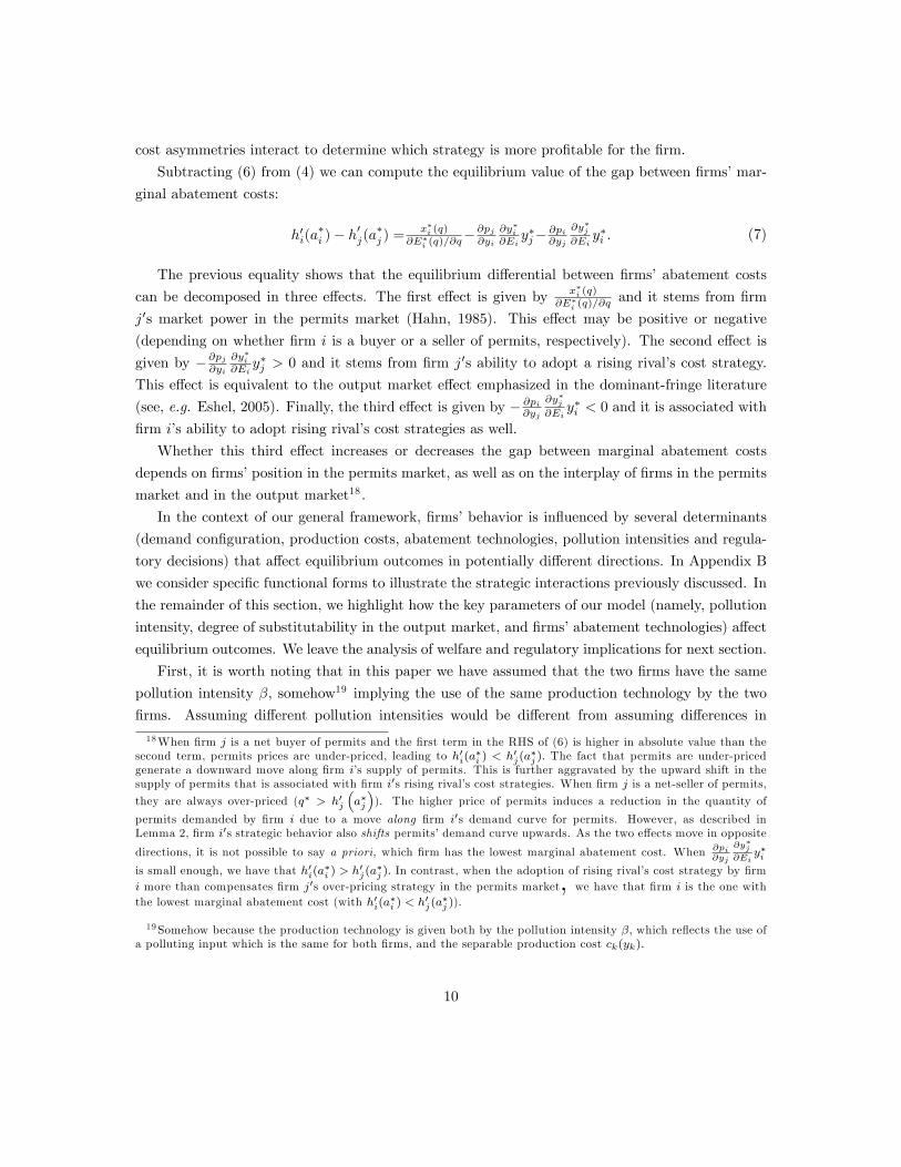
Subtracting (6) from (4) we can compute the equilibrium value of the gap between �rms�mar-
ginal abatement costs:
h0i(a�i )� h
0j(a
�j ) =
x�i (q)@E�
i (q)=@q�@pj@yi
@y�i@Eiy�j�
@pi@yj
@y�j@Eiy�i : (7)
The previous equality shows that the equilibrium di¤erential between �rms�abatement costs
can be decomposed in three e¤ects. The �rst e¤ect is given by x�i (q)@E�
i (q)=@qand it stems from �rm
j0s market power in the permits market (Hahn, 1985). This e¤ect may be positive or negative
(depending on whether �rm i is a buyer or a seller of permits, respectively). The second e¤ect is
given by �@pj@yi
@y�i@Eiy�j > 0 and it stems from �rm j0s ability to adopt a rising rival�s cost strategy.
This e¤ect is equivalent to the output market e¤ect emphasized in the dominant-fringe literature
(see, e.g. Eshel, 2005). Finally, the third e¤ect is given by � @pi@yj
@y�j@Eiy�i < 0 and it is associated with
�rm i�s ability to adopt rising rival�s cost strategies as well.
Whether this third e¤ect increases or decreases the gap between marginal abatement costs
depends on �rms�position in the permits market, as well as on the interplay of �rms in the permits
market and in the output market18 .
In the context of our general framework, �rms�behavior is in�uenced by several determinants
(demand con�guration, production costs, abatement technologies, pollution intensities and regula-
tory decisions) that a¤ect equilibrium outcomes in potentially di¤erent directions. In Appendix B
we consider speci�c functional forms to illustrate the strategic interactions previously discussed. In
the remainder of this section, we highlight how the key parameters of our model (namely, pollution
intensity, degree of substitutability in the output market, and �rms�abatement technologies) a¤ect
equilibrium outcomes. We leave the analysis of welfare and regulatory implications for next section.
First, it is worth noting that in this paper we have assumed that the two �rms have the same
pollution intensity �, somehow19 implying the use of the same production technology by the two
�rms. Assuming di¤erent pollution intensities would be di¤erent from assuming di¤erences in
18When �rm j is a net buyer of permits and the �rst term in the RHS of (6) is higher in absolute value than thesecond term, permits prices are under-priced, leading to h0i(a
�i ) < h0j(a
�j ): The fact that permits are under-priced
generate a downward move along �rm i�s supply of permits. This is further aggravated by the upward shift in thesupply of permits that is associated with �rm i0s rising rival�s cost strategies. When �rm j is a net-seller of permits,
they are always over-priced (q� > h0j
�a�j
�). The higher price of permits induces a reduction in the quantity of
permits demanded by �rm i due to a move along �rm i0s demand curve for permits. However, as described inLemma 2, �rm i0s strategic behavior also shifts permits�demand curve upwards. As the two e¤ects move in opposite
directions, it is not possible to say a priori, which �rm has the lowest marginal abatement cost. When @pi@yj
@y�j@Ei
y�iis small enough, we have that h0i(a
�i ) > h
0j(a
�j ): In contrast, when the adoption of rising rival�s cost strategy by �rm
i more than compensates �rm j0s over-pricing strategy in the permits market, we have that �rm i is the one withthe lowest marginal abatement cost (with h0i(a
�i ) < h
0j(a
�j )).
19Somehow because the production technology is given both by the pollution intensity �; which re�ects the use ofa polluting input which is the same for both �rms, and the separable production cost ck(yk):
10

abatement technologies and cannot be fully captured by using simple scale factors in the abatement
function. It is therefore worth discussing what would be the e¤ect of having a �rm using a less
polluting production process. Everything else the same, a lower � would shift outwards the reaction
function in the output market of the less polluting �rm (and make it �atter). The result would be
that the less polluting �rm would produce more in equilibrium, for any given amount of permits
held, and the most polluting �rm would produce less.
As for the permits market, we �rst explore the case in which �rm i has a lower pollution intensity
than �rm j. Looking at equation (4), when comparing the results with �rm i having a lower � we
can identify a direct e¤ect, for which �rm i is willing to accept a lower price for the supply of any
amount of permits (and is therefore willing to sell more permits for any given price q): h0i decreases
with a lower pollution intensity. However there is also a strategic e¤ect which goes in the opposite
direction.20 In equation (4) the term on the RHS increases with a lower � since y�i is larger for any
given Ei. This term shows that the less polluting �rm is willing to withhold permits in order to
gain a strategic advantage in the output market.
The same reasoning can be done in the case in which �rm j has a pollution intensity that is lower
than �rm i. Looking at (6) we see that there is a direct e¤ect of a lower � on the demand of permits
by �rm j that would choose a lower q (and therefore a lower Ej) on the supply schedule of �rm i
because of its lower marginal abatement cost h0j . As in the case of �rm i there is also a strategic
e¤ect related to the rising-rival-cost strategy of �rm j. The �rm with lower � has an incentive to
withhold pollution permits in order to gain an advantage on the output market. Everything else
the same, the term on the RHS of (6) increases with a lower � since y�j is larger for any given Ei.
Regarding the degree of product di¤erentiation in the output market, it a¤ects �rms�optimal
decisions not only in the output market but also in the permits market. As shown in (4), the degree
of substitutability between good i and j determines the magnitude of q-h0i for �rm i. Similarly, the
degree of substitutability between good j and i determines the magnitude of the �rst term in (6).
When products are very di¤erentiated, a reduction in �rms�marginal abatement cost has a lower
impact on �rms�relative competitiveness in the output market than in the case of close substitutes.
Accordingly, when products are signi�cantly di¤erentiated, the rival�s cost-rising strategies tend to
become less e¤ective and the equilibrium price of permits is mostly in�uenced by �rm j0s position in
the permits market. Instead, when products are close substitutes21 , �rms�relative competitiveness
in the output market depends more signi�cantly on their marginal abatement cost and therefore
�rm j tends to mark up the price of permits to decrease its abatement needs (while increasing the
rival�s abatement needs) and become more competitive in the output market.
The asymmetry between marginal abatement cost functions also a¤ect the relative magnitude
of the two e¤ects in (6) and, as we will see in the following section, the optimal allocation of
20We thank an anonimous referee for pointing out this e¤ect.21This is the case of De Feo et al. (2012) who consider perfectly substitute goods.
11
permits between �rms. As the relative size of the permits market increases in relation to the output
market, if �rm j is a net buyer of permits, it tends to be more interested in marking-down the price
of permits than in increasing its rival�s cost in the output market.
3. REGULATION AND POLICY IMPLICATIONS
From Lemma 2, we conclude that strategic interaction in the output market results in an upward
shift of �rm i0s demand curve (or supply curve) of permits, which leads �rm i to under-invest in
pollution abatement, for any given price of permits. Depending on the interplay between the market
power in the permits market and the incentive to adopt a rival�s cost-rising strategy, �rm j might
be interested in abating more or less than e¢ ciently.
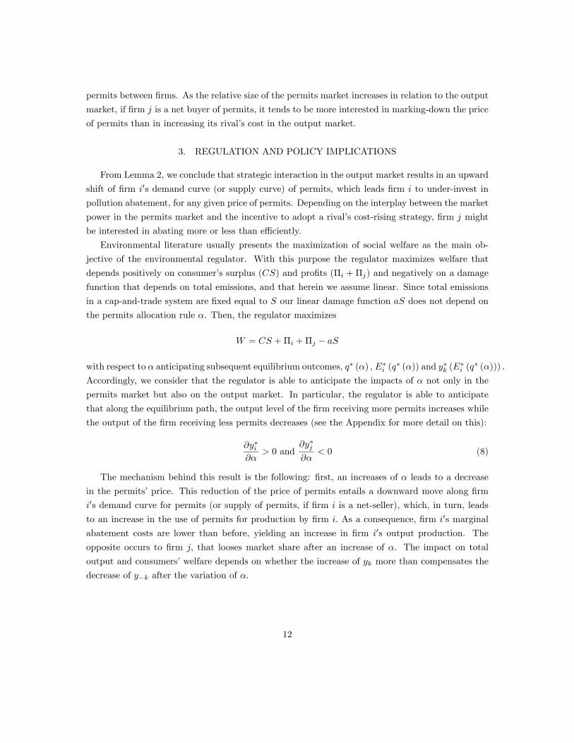
Environmental literature usually presents the maximization of social welfare as the main ob-
jective of the environmental regulator. With this purpose the regulator maximizes welfare that
depends positively on consumer�s surplus (CS) and pro�ts (�i + �j) and negatively on a damage
function that depends on total emissions, and that herein we assume linear. Since total emissions
in a cap-and-trade system are �xed equal to S our linear damage function aS does not depend on
the permits allocation rule �. Then, the regulator maximizes
W = CS +�i +�j � aS
with respect to � anticipating subsequent equilibrium outcomes, q� (�) ; E�i (q� (�)) and y�k (E
�i (q
� (�))) :
Accordingly, we consider that the regulator is able to anticipate the impacts of � not only in the
permits market but also on the output market. In particular, the regulator is able to anticipate
that along the equilibrium path, the output level of the �rm receiving more permits increases while
the output of the �rm receiving less permits decreases (see the Appendix for more detail on this):
@y�i@�
> 0 and@y�j@�
< 0 (8)
The mechanism behind this result is the following: �rst, an increases of � leads to a decrease
in the permits�price. This reduction of the price of permits entails a downward move along �rm
i0s demand curve for permits (or supply of permits, if �rm i is a net-seller), which, in turn, leads
to an increase in the use of permits for production by �rm i: As a consequence, �rm i0s marginal
abatement costs are lower than before, yielding an increase in �rm i0s output production. The
opposite occurs to �rm j; that looses market share after an increase of �. The impact on total
output and consumers�welfare depends on whether the increase of yk more than compensates the
decrease of y�k after the variation of �:
12

Give the regulator�s maximization problem, the following FOC is valid for interior solutions22 :
@CS
@�+@�i@�
+@�j@�
= 0
In Appendix C we show how the previous FOC results in the following optimal permits allocation
rule in the case of symmetric demands in the output market:
dE�id�
�h0i � h0j
�=dE�id�
�@y�i@Ei
y�i@pi@yi
+@y�j@Ei
y�j@pj@yj
�: (9)
Basically such allocation rule ensures that any asymmetry on �rms�equilibrium marginal abate-
ment costs is compensated by an equal asymmetry in the strategic e¤ect on the output market in
equilibrium.
The result in (9) violates the so-called equimarginal principle that has been generally adopted
by the environmental literature (see for example Requate, 2005) that assumes perfect competition
in the market that is subject to the environmental regulation (see for example Montgomery, 1972).
Under perfect competition in the output market equimarginality ensures the minimization of total
abatement costs and, consequently, maximization of total welfare. Due to the strategic interaction in
the output market our result di¤ers from the equimarginal principle. In fact (9) can be reformulated
as we do in the following proposition.
Proposition 1. The optimal allocation of permits is the one that ensures that the di¤erence
on each �rm�s price-cost margins in the permits and in the output market are equalized for the last
permit distributed: ��q � h0j
��@y�j@Ej
��j
�dE�id�
=
�(q � h0i)�
@y�i@Ei
��i
�dE�id�
(10)
where we note markups as ��j =�p�j � c0j � �h0j
�and ��i = (p
�i � c0i � �h0i) respectively.
Proof. See Appendix C.
From Proposition 1 it follows that the optimal allocation of permits is the one guaranteeing
that, for the last permit distributed, the di¤erence on each �rm´s price-cost margin in the permits
market is balanced with the di¤erence on each �rm�s mark-up in the output market, where the
latter is weighted by @y�k@Ek
which measures the e¤ect of the allocation on �rm�s output production.
From (10) we get
h0i � h0j =@y�j@Ej
��j �@y�i@Ei
��i : (11)
22Our analysis is only valid when the conditions that guarantee the existence of an interior solution exist. In ourgeneral setup it is not possible to derive explicitly the conditions that guarantee that an interior solution exists.Whenerver existence conditions for an interior solution are violated, a corner solution arises and the regulator mustallocate all the available emission permits to only one of the �rms.
13

The gap in marginal abatement costs must compensate for the relative strength of �rms�strategic
e¤ects in the output market. For each �rm k; the strategic e¤ect is captured by @y�k@Ek
��k, which
measures the marginal pro�tability obtained by �rm k in the output market when it uses an
additional permit in production. When �rm j0s strategic e¤ect@y�j@Ej
��j > 0 is higher than the one
of �rm i; given by @y�i@Ei��i > 0; the regulator should allocate permits so that h
0i > h
0j : The opposite
occurs when �rm i0s strategic e¤ect is stronger than the one of �rm j:
Note that, for �rm k; the marginal pro�tability of receiving an additional permit to use in
production is given by the savings in the marginal abatement cost h0k plus the marginal pro�tability
of the output increase that such permit will generate, that is entailed by strategic interaction and
it is given by @y�k@Ek
��k in our set-up. Accordingly, an alternative approach to interpret the condition
(11) is to state that the welfare maximizing permits�allocation must equalize �rms�total marginal
pro�tability of receiving an additional permit, as can be seen from restating (11) as
h0i +@y�i@Ei
��i = h0j +
@y�j@Ej
��j :
A regulator that considers strategic interaction in the output market is neglected would allocate
permits so as to ensure equimarginality of abatement costs. For the sake of comparison let us note
the equimarginal allocation rule as �EM , which solves:23
@pj@yi
@y�i@Ei
y�j +@pi@yj
@y�j@Ei
y�i =S�EM � E�i (q)@E�i (q)=@q
: (12)
Recall that the sign of the LHS of (12) is a priori undetermined. The term associated with �rm
j0s rising cost-e¤ect, @pj@yi
@y�i@Eiy�j ; is negative, whereas the term associated with �rm i�s rising-cost
e¤ect, @pi@yj
@y�j@Eiy�i ; is positive. When the �rst term is dominant, so that @pi
@yj
@y�j@Eiy�i < �@pj
@yi
@y�i@Eiy�j ;
the LHS of (12) is negative. This takes place, when one or more of the following occurs:��� @pi@yj
���is su¢ ciently smaller than
���@pj@yi
���; the equilibrium output of �rm i is lower than the equilibrium
output of �rm j, and/ or �rm i0s abatement technology is signi�cantly less e¢ cient than the one of
�rm j: In this case, the equimarginal allocation rule distributes more permits to �rm i (recall that
@E�i (q)=@q is negative). By making �rm i a net-seller of permits, the regulator is inducing �rm j to
buy permits in the market and therefore, �rm j will have additional incentives to mark-down the
price of permits (this corresponds to the e¤ect x�i@E�
i =@q, in equation (6)). This partially o¤sets the
strength of �rm j�s rival�s cost rising e¤ect, restoring equimarginality of abatement. The opposite
situation takes place when the strength of the rising rival�s cost e¤ect is higher for �rm i than
for �rm j (which occurs, for example, when �rm i is endowed with a more e¢ cient abatement
23To obtain condition (12), let us consider the results in the �rst and second stage of the game and substract
equations such that h0i�a�i�= h0j
�a�j
�:
14
technology). In that case the LHS of (12) is positive and equimarginality requires �rm j to be a
net-seller of permits. By doing this, the regulator ensures that �rm j will set a positive mark-up
on the price of permits, which countervails the strength of �rm i0s rival�s rising cost e¤ect.
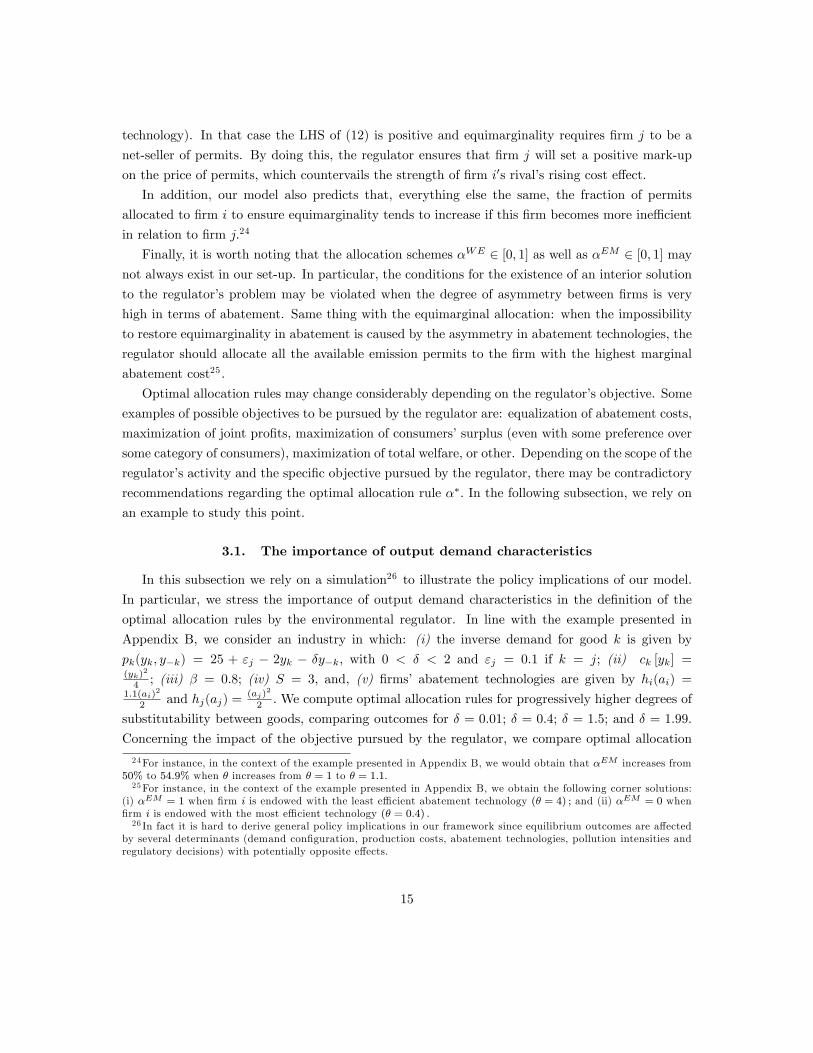
In addition, our model also predicts that, everything else the same, the fraction of permits
allocated to �rm i to ensure equimarginality tends to increase if this �rm becomes more ine¢ cient
in relation to �rm j:24
Finally, it is worth noting that the allocation schemes �WE 2 [0; 1] as well as �EM 2 [0; 1] maynot always exist in our set-up. In particular, the conditions for the existence of an interior solution
to the regulator�s problem may be violated when the degree of asymmetry between �rms is very
high in terms of abatement. Same thing with the equimarginal allocation: when the impossibility
to restore equimarginality in abatement is caused by the asymmetry in abatement technologies, the
regulator should allocate all the available emission permits to the �rm with the highest marginal
abatement cost25 .
Optimal allocation rules may change considerably depending on the regulator�s objective. Some
examples of possible objectives to be pursued by the regulator are: equalization of abatement costs,
maximization of joint pro�ts, maximization of consumers�surplus (even with some preference over
some category of consumers), maximization of total welfare, or other. Depending on the scope of the
regulator�s activity and the speci�c objective pursued by the regulator, there may be contradictory
recommendations regarding the optimal allocation rule ��: In the following subsection, we rely on
an example to study this point.
3.1. The importance of output demand characteristics
In this subsection we rely on a simulation26 to illustrate the policy implications of our model.
In particular, we stress the importance of output demand characteristics in the de�nition of the
optimal allocation rules by the environmental regulator. In line with the example presented in
Appendix B, we consider an industry in which: (i) the inverse demand for good k is given by
pk(yk; y�k) = 25 + "j � 2yk � �y�k; with 0 < � < 2 and "j = 0:1 if k = j; (ii) ck [yk] =(yk)
2
4 ; (iii) � = 0:8; (iv) S = 3; and, (v) �rms� abatement technologies are given by hi(ai) =1:1(ai)
2
2 and hj(aj) =(aj)
2
2 :We compute optimal allocation rules for progressively higher degrees of
substitutability between goods, comparing outcomes for � = 0:01; � = 0:4; � = 1:5; and � = 1:99.
Concerning the impact of the objective pursued by the regulator, we compare optimal allocation
24For instance, in the context of the example presented in Appendix B, we would obtain that �EM increases from50% to 54:9% when � increases from � = 1 to � = 1:1.25For instance, in the context of the example presented in Appendix B, we obtain the following corner solutions:
(i) �EM = 1 when �rm i is endowed with the least e¢ cient abatement technology (� = 4) ; and (ii) �EM = 0 when�rm i is endowed with the most e¢ cient technology (� = 0:4) :26 In fact it is hard to derive general policy implications in our framework since equilibrium outcomes are a¤ected
by several determinants (demand con�guration, production costs, abatement technologies, pollution intensities andregulatory decisions) with potentially opposite e¤ects.
15

rules under four di¤erent regulatory objectives: (i) equimarginality of abatement e¤ort (EM); (ii)
maximization of �rms� joint pro�ts (JP ); and, �nally, (iii) maximization of total social welfare
(W ). To compute consumer�s surplus, we use the partial equilibrium analysis from Belle�amme
and Peitz (2010). Table 3 summarizes our results:
Substitution EM JP W
� = 0:01 ��EM = 54:1% ��JP = 54% ��W = 69%
� = 0:4 ��EM = 54:4% ��JP = 53% ��W = 61%
� = 1:5 ��EM = 54:9% ��JP = 51% ��W = 60%
� = 1:99 ��EM = 55:2% ��JP = 51% ��W = 60%
Table 3: Optimal permits allocations
Reading each line separately, we conclude that the optimal allocation of permits varies according
to the regulator�s objective. When the regulator wants to promote equimarginality of pollution
abatement (EM), he voluntarily chooses to ignore the impact of permits decisions on the outputmarket. Table 3 shows that, under a equimarginality allocation rule, the regulator must allocate
more permits to the �rm that owns the less e¢ cient abatement technology (as described in the
previous section). In relation to the way output market characteristics in�uence the equimarginality
allocation rule, table 3 shows that as substitutability decreases, rising-rival�s cost strategies are
weaker (due to less competition) and therefore the lower needs to be the compensation27 to the
least e¢ cient �rm. It is worth noting that the equimarginality allocation rule is not very sensitive
to changes in the degree of output substitutability. In fact output demands remain perfectly
symmetric, with @pi@yj
=@pj@yi
and therefore, the degree of product substitutability only a¤ects the
strength of rival�s cost-rising e¤ects indirectly, through its e¤ect on output production (and therefore
in �rms�abatement needs).
Turning now to the maximization of joint pro�ts (JP), the optimal allocation of permits oncemore favours the least e¢ cient �rm i: This is the case because, when giving more permits to the
least e¢ cient �rm, the increase in its output production (and its pro�ts) more than compensates
the decrease in its rival�s production (and pro�ts). The changes in the pro�t-maximizing allocation
as substitutability changes are stronger than in the cost-e¤ective allocation.
Finally, the welfare maximizing (W) allocation rule gives even more permits to the least e¢ cient
�rm than the pro�t maximizing allocation rule. This is the case because the latter only accounts for
the fact that the increase in the least e¢ cient �rm�s output production after an increase in � more
than compensates the decrease in the most e¢ cient �rm�s output production. Instead, the welfare
maximizing allocation rule also accounts for the fact that the mentioned changes in quantities a¤ect
prices and consequently consumer�s surplus. In particular, for the values of the parameters that we
27Compensation in this context takes place through a higher permits allocation.
16
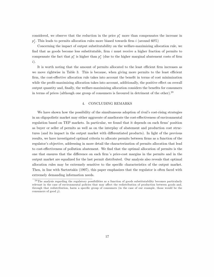
considered, we observe that the reduction in the price p�i more than compensates the increase in
p�j : This leads to permits allocation rules more biased towards �rm i (around 60%)
Concerning the impact of output substitutability on the welfare-maximizing allocation rule, we
�nd that as goods become less substitutable, �rm i must receive a higher fraction of permits to
compensate the fact that p�i is higher than p�j (due to the higher marginal abatement costs of �rm
i).
It is worth noting that the amount of permits allocated to the least e¢ cient �rm increases as
we move rightwise in Table 3. This is because, when giving more permits to the least e¢ cient
�rm, the cost-e¤ective allocation rule takes into account the bene�t in terms of cost minimization
while the pro�t-maximizing allocation takes into account, additionally, the positive e¤ect on overall
output quantity and, �nally, the welfare-maximizing allocation considers the bene�ts for consumers
in terms of prices (although one group of consumers is favoured in detriment of the other).28
4. CONCLUDING REMARKS
We have shown how the possibility of the simultaneous adoption of rival�s cost-rising strategies
in an oligopolistic market may either aggravate of ameliorate the cost-e¤ectiveness of environmental
regulation based on TEP markets. In particular, we found that it depends on each �rms�position
as buyer or seller of permits as well as on the interplay of abatement and production cost struc-
tures (and its impact in the output market with di¤erentiated products). In light of the previous
results, we have investigated optimal criteria to allocate permits between �rms as a function of the
regulator�s objective, addressing in more detail the characterization of permits allocation that lead
to cost-e¤ectiveness of pollution abatement. We �nd that the optimal allocation of permits is the
one that ensures that the di¤erence on each �rm´s price-cost margins in the permits and in the
output market are equalized for the last permit distributed. Our analysis also reveals that optimal
allocation rules may be extremely sensitive to the speci�c characteristics of the output market.
Then, in line with Sartzetakis (1997), this paper emphasizes that the regulator is often faced with
extremely demanding information needs.
28The analysis regarding the regulatory possibilities as a function of goods substitutability becomes particularlyrelevant in the case of environmental policies that may a¤ect the redistribution of production between goods and,through that redistribution, harm a speci�c group of consumers (in the case of our example, those would be theconsumers of good j).
17

REFERENCES
[1] Belle�amme, P and Peitz, M. [2010] Industrial Organization Markets and Strategies, Cam-
bridge University Press.
[2] Amir, R. [2005]. Supermodularity and Complementarity in Economics: An Elementary Survey,
Southern Economic Journal, 71(3), 636-660.
[3] Chen, Y., Hobbs, B.F., Ley¤er, S. and Munson T.S., [2006], Leader-follower equilibria for
electric power and NOx allowances markets, Computational Managment Science, 3, 307�330.
[4] G. de Feo, J. Resende, M-E Sanin, [2012], Emission permits trading and downstream strategic
interaction, forthcoming The Manchester School.
[5] D. M. D. Eshel, [2005], Optimal allocation of tradable pollution rights and market structures,
Journal of Regulatory Economics, 28:2, 205-223.
[6] Fehr, N.-H. M. v. d. [1993], Tradable Emission Rights and Strategic Interaction, Environmental
and Resource Economics, 3, 129-151.
[7] Hahn, R. [1985], Market power and transferable property rights. Quarterly Journal of Eco-
nomics, 99, 753�765.
[8] IPCC [1990], Climate change: The IPCC Scienti�c Assessment.
[9] Kolstad, J. and F. Wolak, [2008], Using emission permits prices to rise electricity prices: Evi-
dence from the California electricity market, Harvard University, mimeo.
[10] Liski, M and Juan-Pablo Montero, [2011], Market Power in an Exhaustible Resource Market:
The Case of Storable Pollution Permits, Economic Journal, 121(551), 116-144.
[11] Misiolek, W. S. and H. W. Elder [1989], Exclusionary manipulation of markets of pollution
rights. Journal of Environmental Economics and Management, 16, 156-166.
[12] Montero, J.P. [2009], Market Power in Pollution Permit Markets. The Energy Journal, 30(Special I), 115-142.
[13] Montgomery, D. W. [1972], Market in Licenses and E¢ cient Pollution Control Programs,
Journal of Economic Theory, 395-418.
[14] Requate, T. [2005]. Timing and Commitment of Environmental Policy, Adoption of New Tech-
nology, and Repercussions on R&D, Environmental & Resource Economics, 31(2), 175-199,06.
18
[15] Salop, S.C. and D.T. Sche¤man [1983], Raising rivals�costs, American Economic Review Papers
and Proceedings, 73, 267-271.
[16] Sartzetakis E.S. [1997], Tradable Emission Permits Regulations in the Presence of Imperfectly
Competitive Product Markets: Welfare Implications, Environmental and Resource Economics,
9, 65-81.
[17] Tanaka, M. and Y. Chen [2012], Emissions Trading in Forward and Spot Markets of Electricity,
The Energy Journal, 33(2)
[18] Wolak, F.A. [2003b], Measuring Unilateral Market Power in Wholesale Electricity Markets:
The California Market 1998 to 2000, American Economic Review, May, 425-430.
19

Appendix A
Proof of Lemma 1By applying the theory of supermodular games, the sign of the e¤ect of Ek on yk and y�k depends
on the sign of the cross-partial derivatives @2�k@yk@Ek
and @2��k@y�k@Ek
.29 Without loss of generality,
suppose k = i. Since@2�i@yi@Ei
= �h00i (�yi�Ei) > 0
and@2�j@yj@Ei
= ��h00j (�yj�S + Ei) < 0
the larger Ei, the larger y�i (Ei) and the smaller y�j (Ei).
SOC of the second-stage optimization problemThe second order condition of the problem can be written as
d2�idE2i
=@ (d�i=dEi)
@Ei+@ (d�i=dEi)
@y?i
@y?i@Ei
+@ (d�i=dEi)
@y?j
@y?j@Ei
where the �rst term is:
@ (d�i=dEi)
@Ei=
�@y?i@Ei
� 1�h00i (�y
?i � Ei) +
@Pi�y?i ; y
?j
�@y?j
@y?j@Ei
;
the second term is:
@ (d�i=dEi)
@y?i
@y?i@Ei
=
"�h00i (�y
?i � Ei) + 2
@pi�y?i ; y
?j
�@y?i
� c00i (y?i )� �2h00i (�y?i � Ei)#@y?i@Ei
;
and �nally the third term is:
@ (d�i=dEi)
@y?j
@y?j@Ei
=@pi
�y?i ; y
?j
�@y?i
@y?i@Ei
@y?i@Ei
:
Therefore the SOC can be written as follows:��1� �2 + �
� @y?i@Ei
� 1�h00i (�y
?i � Ei)+
@pi�y?i ; y
?j
�@y?i
@y?i@Ei
�1 +
@y?i@Ei
�+
"2@pi
�y?i ; y
?j
�@y?i
� c00i (y?i )#@y?i@Ei
< 0
Proof of (8)
29See Amir (2005) for a survey of this approach.
20

Applying the chain rule, the derivatives @y�k@� can be decomposed as follows:
@y�k@�
=@y�k(q; Ei)
@Ei
@E�i (q)
@q
@q�
@�;
where the derivatives @y�k(q;Ei)@Ei
have already been obtained in Lemma , with @y�k(Ek)@Ek
> 0;and@y��k(Ek)
@Ek< 0: We have also seen that @E�
i
@q < 0 because @2�i@Ei@q
< 0: Similarly, @q�
@� < 0 because@2�j@q@� < 0 (complementarity and supermodularity, see Amir, 2005).
Accordingly, along the equilibrium path
@y�i@� =
@y�i (q;Ei)@Ei
@E�i (q)@q
@q�
@� > 0;
and@y�j@� =
@y�i (q;Ei)@Ei
@E�i (q)@q
@q�
@� < 0:
As stated in (8) after a marginal variation of �; the equilibrium output of �rm i changes in the
same direction, while the equilibrium output of �rm j changes in the opposite direction.
Appendix B: an example
Herein we rely on an example to illustrate how relevant parameters, such as �rms� relative
e¢ ciency in terms of abatement, may a¤ect equilibrium market outcomes.30 We consider that (i)
the inverse demand for good k is given by pk(yk; y�k) = 25 � 2yk � 1:5y�k; (ii) �rms�productiontechnology is similar, with ck [yk] =
(yk)2
4 ; (iii) the intensity of pollution is equal to � = 0:8; (iv) the
total stock of emission permits is exogenously �xed by the regulator to meet the pollution control
target and we consider it to be S = 3; which constrains �rms�production plans. Finally, (v) �rms�
abatement technologies are given by hi(ai) =�(ai)
2
2 and hj(aj) =(aj)
2
2 :
In what follows, we compute the equilibrium outcomes as in Section 2.1 considering the speci�c
functions detailed in points (i) to (v). Regarding �rm i0s abatement technology, we consider three
possible scenarios: �rm i is more e¢ cient in terms of abatement (� = 0:4); �rms have symmetric
abatement technologies (� = 1); and �rm j is more e¢ cient in terms of abatement (� = 4) : In the
following table we reproduce the predictions of our model regarding equilibrium prices (both for
30Note that a similar analysis could be performed to study the in�uence of other parameters, such as outputdemand, production costs or the pollution cap S:For the sake of simplicity, in the paper we present only an examplethat analyses the e¤ects of abatement technologies and, at the end of the section, we comment on other potentiallyrelevant parameters.
21

permits and output) and equilibrium trading levels for di¤erent values of �:
p�i p�j q� x�i
� = 0:4 10:9 + 0:02� 10:9 + 0:13� 2:1� 0:21� 2: 3�� 0:9� = 1 11:2� 0:11� 11:2� 0:11� 3: 3� 0:75� 2:0�� 1:0� = 4 12:4� 0:78� 11:8� 0:22� 7: 1� 2:81� 1:7�� 1:1
Table B: Equilibrium outcomes � = 0:4; � = 1; � = 4
Table B shows that equilibrium output prices depend on �rms�abatement technologies. As we
would expect, since �rms are symmetric with respect to everything else except abatement e¢ ciency,
the �rm with the most e¢ cient abatement technology has a competitive advantage in the output
market o¤ering its product as a lower price. Furthermore, Table B shows that an increase in � leads
to an increase in the output price of both goods. The regulator can partially o¤set this increase by
allocating more permits to �rm i when this �rm becomes progressively more ine¢ cient. In a quite
di¤erent context Tanaka and Chen (2012) �nd a contrasting result, which underlines the importance
of taking into account the market structure as a key variable to choose optimal permits allocation.
Regarding permits�trading, Table B shows that �rm i might be a net buyer or seller, depending
on the value of �: For example, if � < 0:39; �rm i is always a net buyer of permits, for the three
technological speci�cations. In contrast, if � > 0:65; �rm i is always a net seller of permits, for
the three technological speci�cations. For intermediate values of �; �rm i is a net seller only for
some speci�cations of the abatement cost function. As expected, when �rm i becomes relatively less
e¢ cient than �rm j; it sells less (or buys more) permits to compensate its lower abatement e¢ ciency
and become more competitive in the output market (in other words, �rm i is adopting a rival�s
rising-cost strategy). In what concerns the price of permits, when �rm i becomes relatively less
e¢ cient than �rm j; Table B shows an increase in the price of permits. As we move from � = 0:4
to � = 4; and �rm i becomes more ine¢ cient, �rm j increases the price of permits to withhold
permit emissions and avoid the e¤ects of �rm i0s rival�s rising-cost strategies in the second stage. It
is worth noting that herein we just consider technological speci�cations for which q� ��h0j��> 0;
meaning that even when �rm j is a net buyer of permits, the rival�s rising cost e¤ect is always
dominant.
Appendix C: Social Optimum
The regulator�s problem is to maximize (assuming a linear damage function aS) W = CS +
�i +�j � aS with respect to �: Whenever interiority conditions are met, the FOC to the previousproblem is given by @CS
@� + @�i@� +
@�j@� = 0: Let us now compute each of the derivatives herein.
Consumer Surplus
22
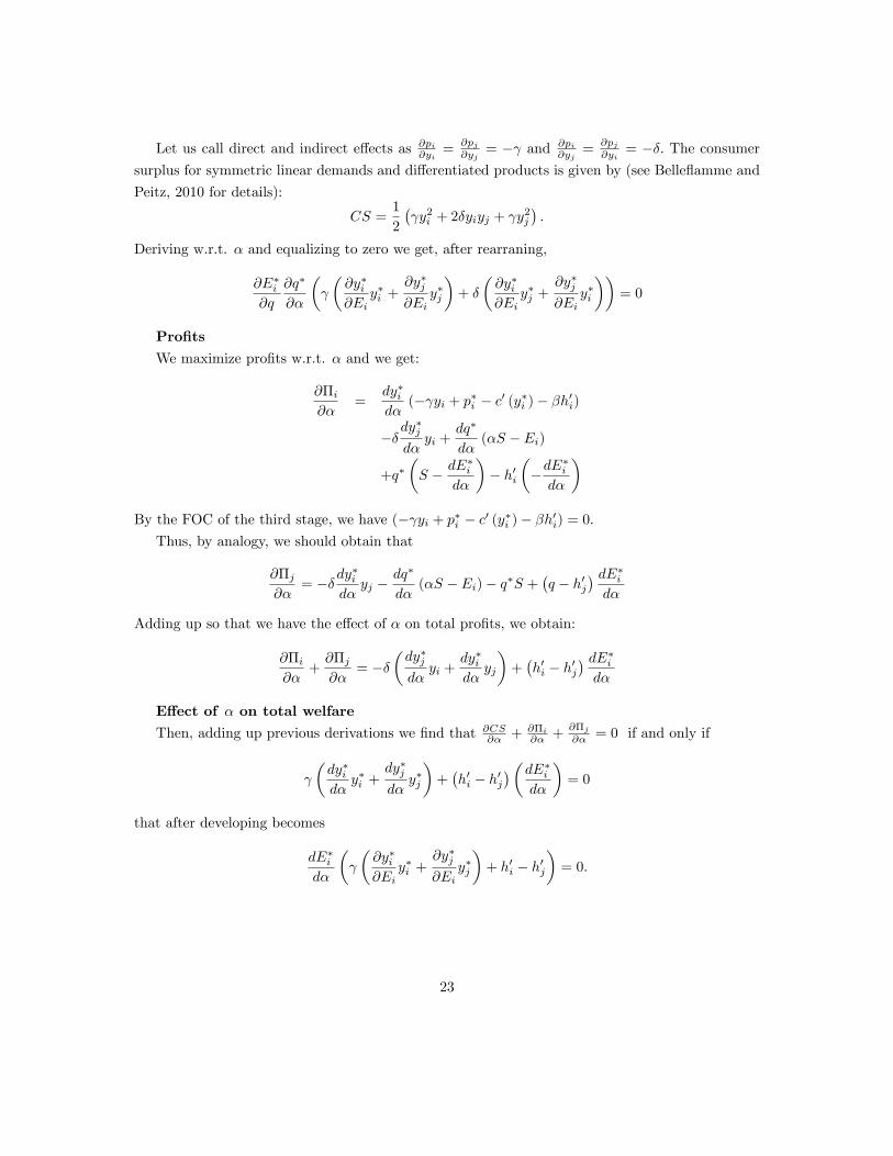
Let us call direct and indirect e¤ects as @pi@yi
=@pj@yj
= � and @pi@yj
=@pj@yi
= ��: The consumersurplus for symmetric linear demands and di¤erentiated products is given by (see Belle�amme and
Peitz, 2010 for details):
CS =1
2
� y2i + 2�yiyj + y
2j
�:
Deriving w.r.t. � and equalizing to zero we get, after rearraning,
@E�i@q
@q�
@�
�
�@y�i@Ei
y�i +@y�j@Ei
y�j
�+ �
�@y�i@Ei
y�j +@y�j@Ei
y�i
��= 0
Pro�tsWe maximize pro�ts w.r.t. � and we get:
@�i@�
=dy�id�
(� yi + p�i � c0 (y�i )� �h0i)
��dy�jd�yi +
dq�
d�(�S � Ei)
+q��S � dE
�i
d�
�� h0i
��dE
�i
d�
�By the FOC of the third stage, we have (� yi + p�i � c0 (y�i )� �h0i) = 0.Thus, by analogy, we should obtain that
@�j@�
= �� dy�i
d�yj �
dq�
d�(�S � Ei)� q�S +
�q � h0j
� dE�id�
Adding up so that we have the e¤ect of � on total pro�ts, we obtain:
@�i@�
+@�j@�
= ���dy�jd�yi +
dy�id�yj
�+�h0i � h0j
� dE�id�
E¤ect of � on total welfareThen, adding up previous derivations we �nd that @CS@� + @�i
@� +@�j@� = 0 if and only if
�dy�id�y�i +
dy�jd�y�j
�+�h0i � h0j
��dE�id�
�= 0
that after developing becomes
dE�id�
�
�@y�i@Ei
y�i +@y�j@Ei
y�j
�+ h0i � h0j
�= 0:
23

Considering that @pi@yi=
@pj@yj
= � we get equation (9):
dE�id�
�h0i � h0j
�=dE�id�
�@y�i@Ei
y�i@pi@yi
+@y�j@Ei
y�j@pj@yj
�:
The previous can be rearranged considering the following equalities taken from the third stage
equilibrium:
y�i@pi@yi
= � (p�i � c0i � �h0i)
y�j@pi@yi
= ��p�j � c0j � �h0j
�to get
dE�id�
�h0i � h0j
�=dE�id�
��@y�j@Ei
�p�j � c0j � �h0j
�� @y�i@Ei
(p�i � c0i � �h0i)�
Adding and subtracting q dE�i
d� on the LHS and rearranging, we get��q � h0j
��@y�j@Ej
��j
�dE�id�
=
�(q � h0i)�
@y�i@Ei
��i
�dE�id�
where we note markups as ��j =�p�j � c0j � �h0j
�and ��i = (p
�i � c0i � �h0i) respectively.
24