Optical remote sensing for dredge plume monitoring: a review · Department of Physics and Astronomy, Remote Sensing and Satellite Research Group, Science and Engineering, School of

Optical remote sensing for dredge plume monitoring: a review Peter Fearns1,2, Mark Broomhall1,2, Passang Dorji1,2

1 Department of Physics and Astronomy, Remote Sensing and Satellite Research Group, Science and Engineering, School of Science, Curtin University, Perth, Western Australia, Australia

2 Western Australian Marine Science Institution, Perth, Western Australia, Australia

WAMSI Dredging Science Node Report

Theme 3 |Project 3.1.1 October 2017

http://www.wamsi.org.au

WAMSI Dredging Science Node

The WAMSI Dredging Science Node is a strategic research initiative that evolved in response to uncertainties in the environmental impact assessment and management of large-scale dredging operations and coastal infrastructure developments. Its goal is to enhance capacity within government and the private sector to predict and manage the environmental impacts of dredging in Western Australia, delivered through a combination of reviews, field studies, laboratory experimentation, relationship testing and development of standardised protocols and guidance for impact prediction, monitoring and management.

Ownership of Intellectual property rights

Unless otherwise noted, any intellectual property rights in this publication are owned by the Western Australian Marine Science Institution and Curtin University.

Copyright

© Western Australian Marine Science Institution

All rights reserved.

Unless otherwise noted, all material in this publication is provided under a Creative Commons Attribution 3.0 Australia Licence. (http://creativecommons.org/licenses/by/3.0/au/deed.en)

Funding Sources

The $20million Dredging Science Node is delivering one of the largest single issue environmental research programs in Australia. This applied research is funded by Woodside Energy, Chevron Australia, BHP Billiton and the WAMSI Partners and designed to provide a significant and meaningful improvement in the certainty around the effects, and management, of dredging operations in Western Australia. Although focussed on port and coastal development in Western Australia, the outputs will also be broadly applicable across Australia and globally.

This remarkable collaboration between industry, government and research extends beyond the classical funder-provider model. End-users of science in regulator and conservation agencies, and consultant and industry groups are actively involved in the governance of the node, to ensure ongoing focus on applicable science and converting the outputs into fit-for-purpose and usable products. The governance structure includes clear delineation between end-user focussed scoping and the arms-length research activity to ensure it is independent, unbiased and defensible.

And critically, the trusted across-sector collaboration developed through the WAMSI model has allowed the sharing of hundreds of millions of dollars’ worth of environmental monitoring data, much of it collected by environmental consultants on behalf of industry. By providing access to this usually confidential data, the Industry Partners are substantially enhancing WAMSI researchers’ ability to determine the real-world impacts of dredging projects, and how they can best be managed. Rio Tinto's voluntary data contribution is particularly noteworthy, as it is not one of the funding contributors to the Node.

Funding and critical data Critical data

http://creativecommons.org/licenses/by/3.0/au/deed.en

Legal Notice

The Western Australian Marine Science Institution advises that the information contained in this publication comprises general statements based on scientific research. The reader is advised and needs to be aware that such information may be incomplete or unable to be used in any specific situation. This information should therefore not solely be relied on when making commercial or other decision. WAMSI and its partner organisations take no responsibility for the outcome of decisions based on information contained in this, or related, publications.

Year of publication: 2017

Metadata: http://catalogue.aodn.org.au/geonetwork/srv/eng/metadata.show?uuid=de2bdcc7-909d-462b-9252-997df88cefba

Citation: Fearns P, Broomhall M, Dorji P (2017) Optical remote sensing for dredge plume monitoring: a review. Report of Theme 3 - Project 3.1.1, prepared for the Dredging Science Node, Western Australian Marine Science Institution, Perth, Western Australia, 46 pp.

Author Contributions: PF, MB and PD all contributed to the writing of this report.

Corresponding author and Institution: P. Fearns (Curtin). Email address: [email protected]

Competing Interests: The commercial investors and data providers had no role in the data analysis, data interpretation, the decision to publish or in the preparation of the manuscript. The authors have declared that no competing interests exists.

Acknowledgements: None

Collection permits/ethics approval: No collection occurred in the production of this report.

Front cover images (L-R)

Image 1: Trailer Suction Hopper Dredge Gateway in operation during the Fremantle Port Inner Harbour and Channel Deepening Project. (Source: OEPA)

Image 2: Passang Dorji collecting water samples in the field to determine the level of total suspended solids (TSS) in the water column to calibrate remotely sensed TSS maps. (Source: Kevin Crane)

Image 3: Dredge plume at Barrow Island. Image produced with data from the Japan Aerospace Exploration Agency (JAXA) Advanced Land Observing Satellite (ALOS) taken on 29/08/2010.

Image 4: Map showing light available at the substrate derived from satellite image. Products such as these could be used to monitor the risk of impacts to photosynthetic organisms such as seagrass during dredge programs. (Source: Curtin University)

mailto:[email protected]

Dredging Science Node | Theme 3 | Project 3.1.1

Contents EXECUTIVE SUMMARY ...................................................................................................................................... I

CONSIDERATIONS FOR PREDICTING AND MANAGING THE IMPACTS OF DREDGING ......................................... I

GLOSSARY ........................................................................................................................................................ 1

1 INTRODUCTION ....................................................................................................................................... 1

2 WATER QUALITY, OCEAN OPTICS AND REMOTE SENSING ........................................................................ 3

2.1 WATER QUALITY .........................................................................................................................................3 2.1.1 Turbidity ...........................................................................................................................................3 2.1.2 Total Suspended Sediment ...............................................................................................................4

2.2 WATER OPTICS ...........................................................................................................................................5 2.2.1 Photosynthetically Active Radiation (PAR) .......................................................................................5 2.2.2 Inherent and apparent optical properties (IOPs and AOPs) .............................................................6 2.2.3 Scattering .........................................................................................................................................8 2.2.4 Transmittance.................................................................................................................................10 2.2.5 Absorption ......................................................................................................................................10 2.2.6 Light profiles, attenuation, spectral versus PAR .............................................................................10 2.2.7 Irradiance and Radiance .................................................................................................................11 2.2.8 Irradiance Attenuation ...................................................................................................................11 2.2.9 Reflectance .....................................................................................................................................12

3 REMOTE SENSING PRODUCTS AND ALGORITHMS .................................................................................. 13

3.1 SPACE-BASED SENSORS ...............................................................................................................................14 3.2 APPROACHES USED IN TSS MAPPING .............................................................................................................17 3.3 UTILISING IN SITU MEASUREMENTS TO DEVELOP ALGORITHMS ............................................................................20 3.4 REMOTE SENSING REFLECTANCE AND TSS ......................................................................................................20

4 AVAILABLE DATA ................................................................................................................................... 23

5 DISCUSSION ........................................................................................................................................... 25

6 CONCLUSIONS ........................................................................................................................................ 27

7 REFERENCES ........................................................................................................................................... 28

8 APPENDICES ........................................................................................................................................... 33

APPENDIX 1. THE TABLE BELOW IS ADAPTED FROM MATTHEWS (2011) AND SHOWS THE TSS ALGORITHMS AND THEIR

CHARACTERISTICS FOR A NUMBER OF SENSORS ..............................................................................................................33

Dredging Science Node | Theme 3 | Project 3.1.1

Optical remote sensing for dredge plume monitoring

Dredging Science Node | Theme 3 | Project 3.1.1 i

Executive Summary

This report presents a review of the potential of remote sensing to support dredge plume monitoring, and the availability of existing in situ data that may support further research into the development and validation of applicable remote sensing products.

There is clearly huge potential for using remote sensing for monitoring the spatial and temporal extents of dredge plumes. Remote sensing can also provide an estimate of the intensity of dredge plumes including parameters such as the relative concentrations of sediment, optical properties of the water column, and light at the substrate. Nearly 70 remote sensing algorithms have been identified, all delivering ‘water quality’ products relevant to dredge plume monitoring. The numerous sensors encompass spatial resolutions from a few metres to many hundreds of metres, and temporal sampling at near daily to monthly, or on-demand. It is difficult to provide a definitive statement on the most appropriate sensor for all dredging-related applications; however, with decreasing costs of data access and processing, best-practice approaches in the future will likely involve multiple sensors. For example, high resolution sensors, typically limited by poor temporal coverage and high cost, could be combined with low spatial resolution, near daily data from free data access sensors.

It has been demonstrated definitely that remote sensing can provide relative measures of various water quality parameters, however the accuracy of products must be carefully considered if used for compliance monitoring where it involves determining specific concentrations for example. The highly turbid waters associated with coastal dredge operations are extremely optically complex, thus algorithms are often specific to very localised conditions. Although there is a large suite of existing remote sensing algorithms, the application of any algorithm to a specific location should be undertaken with caution. Existing algorithms should be evaluated for their accuracy prior to their application. In situations where existing algorithms are unsuitable, new algorithms could be developed based on knowledge of local optical conditions, typically derived from in situ sampling.

A suite of in situ data has been identified that could aid in remote sensing algorithm development and validation of existing algorithms.

Considerations for predicting and managing the impacts of dredging

According to the ’National Assessment Guidelines for Dredging‘ (Commonwealth of Australia, 2009) there are two types of monitoring, compliance monitoring and field monitoring: compliance monitoring measures compliance with the approved project and permit conditions, while field monitoring measures the condition, and changes in condition, of the receiving environment. The guidelines include ‘turbidity’ as one of the factors requiring to be monitored. In Western Australia, the environmental impact assessment (EIA) of marine dredging proposals is guided by Technical Guidance: Environmental Impact Assessment of Marine Dredging Proposals (EPA 2016). This approach employs an impact and effects zonation scheme and also differentiates between monitoring for compliance and monitoring to inform the environmental management of dredging operations. This approach relies on being able to identify the zone of influence and distinguish between natural and dredging generated turbidity.

Optical remote sensing methods are very useful in this regard, as they can provide reliable ‘maps’ of plume extent and provide repeated views over large areas, thus providing managers and regulators with synoptic views of areas that have been influenced by dredge operations, and areas that have not.

We have noted in this review that there are a number of measurable parameters related to turbidity, including NTU, TSS, attenuation coefficients KPAR and K490, scattering coefficients, and time series of light logger data. All of these parameters may be measured with in situ instruments, but many may also be inferred from remotely sensed data. NTU sensors are cheap and simple to operate and appear to have been adopted as the standard approach to monitoring turbidity. However, a relationship between NTU and TSS based on in situ sampling, for example, can be quite location specific. In many cases, particularly those involving large scale capital dredging across strong inshore offshore gradients of sediment type, TSS:NTU relationships may need to be assessed on a


ii Dredging Science Node | Theme 3 | Project 3.1.1

project-specific and potentially a site-specific basis.

It is important to consider the intended reason for monitoring turbidity in order to help determine the most applicable method of capture, and the form of the derived products. For example, if the intent is to define the decrease in light levels reaching the seabed then an attenuation coefficient product is directly applicable. If the intent is to determine sediment distribution and fate (e.g. deposition) then TSS is likely to be a more useful and better product.

Remote sensing can provide a much better overview of the spatial extent of dredging plumes compared to data collected from in situ sensors. Historical remote sensing imagery, together with information collected in months to years after dredging, can also provide information on longer term, legacy effects of sediments spilled during dredging, such as the potential for increased turbidity. In particular, satellite remote sensing could also be used to examine the stability and performance of dredge material placement sites months to years after dredging, and whether they are having long-term effects on local water quality. These data, coupled with contemporaneous data on physical forcings such as wind speed and direction, and swell height, can be used to understand the processes involved in resuspension/deposition and inform predictive models of future events.

The issue with remote sensing data is the accuracy or uncertainty of the products. Appendix 1 presents approximately 70 algorithms for remotely sensed turbidity, clarity, attenuation or TSS products. There is no one algorithm that is globally applicable, at least not an algorithm that users can be confident in obtaining consistently reliable results. However, there are well established methods and equipment to support development and monitoring of algorithms suitable for highly turbid conditions. There is potential to develop algorithms and to monitor the accuracy of the products using well defined procedures to not only support monitoring to inform management, but also to support compliance monitoring/decision making.

The light attenuating properties of suspended sediment are well known; however from this review it is clear that much less is known about how suspended sediments affect the spectral quality of the transmitted light. Pigments in marine benthic primary producers such as seagrasses, macroalgae and corals preferentially absorb different parts of the photosynthetically active radiation (PAR) spectrum. If these preferred wavelengths are attenuated by different types of sediments then conventional PAR sensors (which integrate across the entire PAR spectrum) may overestimate the amount of light that can be used in photosynthesis (i.e. photosynthetically useable radiation, PUR) or not capture the variability in spectral quality in inshore-offshore gradients or when different types of sediments are dredged or re-suspended (e.g. siliciclastic versus carbonate and mixed sediments or different colours). Remote sensing techniques have great potential to capture the temporal and spatial variability in spectral quality by using knowledge of the in situ spectral attenuation properties of TSS combined with the remotely sensed TSS to model and predict the spectral quality of the light field in the water column and at the substrate.


Dredging Science Node | Theme 3 | Project 3.1.1 1

Glossary

AOPs apparent optical property CDOM chromophoric dissolved organic matter

DIS Dredging information system Ed downwelling irradiance EM electromagnetic FAU formazin attenuation unit FNU formazin nephelometric unit FTU formazin turbidity unit HRV high resolution visible IRS Indian Remote Sensing IOP inherent optical properties

Kd(λ) is the diffuse attenuation coefficient for downwelling irradiance at wavelength λ KPAR diffuse attenuation coefficient for PAR LISS Linear Imaging Self Scanner (LISS)

LISST laser in situ scattering and transmissometry MERIS medium resolution imaging spectrometer MODIS moderate resolution imaging spectroradiometer, flown on NASA’s Terra and Aqua satellites.

NIR near-infrared NTU nephelometric turbidity unit OBS optical backscatter OLI Operational Land Imager PAR photosynthetically active radiation, solar radiation in the wavelength region of 400-700 nm PUR photosynthetically useable radiation PSD Particle size distribution

RSSRG Remote Sensing and Satellite Research Group, Curtin University Seston mass of non-dissolved solid material floating or suspended within the water column

SPM suspended particulate matter SSC suspended sediment concentration

THEOS Thailand Earth Observation System TSM total suspended matter TSS total suspended sediment or solids

Turbidity a measure of water clarity or cloudiness - how much the material suspended in the water decreases the passage of light through the water

tripton the inorganic component of seston VSF volume scattering function 𝐙𝐙𝐒𝐒𝐒𝐒 Secchi disk depth

1 Introduction

Predicting the distribution and fate of suspended sediment plumes associated with dredge operations is generally achieved by advanced hydrodynamic modelling (GBRMPA, 2012). The accuracy of the model outputs, or the level of confidence we associate with the modelled forecasts, depend to some degree on the model inputs, including parameters such as suspended sediment concentration (SSC), particle size distributions (PSDs), particle densities, and particle settling rates. There is potential to infer optical products from the modeled 3 dimensional plume distribution, including spectral light attenuation, and spectral light intensity at the substrate.

One of the approaches to testing or monitoring the accuracy of plume distribution models is to compare the


2 Dredging Science Node | Theme 3 | Project 3.1.1

modelled distributions to observed plume distributions. Direct sampling via in situ methods can provide accurate measures of plume conditions, but the spatial coverage is typically limited. Optical remote sensing methods can provide reliable ‘maps’ of plume extent, and reasonable estimates of various in-water geophysical parameters. Examples of remote sensing products include suspended sediment concentration, particle backscattering, and spectral light attenuation coefficients. Also, remote sensing technologies typically provide repeated views over large areas, thus providing researchers and managers with synoptic views of ocean regions potentially impacted by dredge operations.

Remote sensing of coastal and marine environments may be carried out by satellite-borne sensors, sensors mounted on aircraft, unmanned airborne vehicles, and sensors mounted on boats. These data may be processed to deliver products in near-real time.

The long lifetime of many earth observing satellite missions has led to the production of significant archives of historical data. These data are available for assessing natural variation in ocean conditions, determining baselines, or for model tuning and validation. By analysing a series of images through time there is potential to derive higher level products, representative of baseline conditions, analyze system processes, circulation patterns etc. Maps of water optical conditions may be combined with bathymetry to infer the light conditions at the substrate.

It is generally accepted that the most accurate measure of water column conditions is achieved through direct measurements based on in situ samples (e.g. TSS determined by filtering and weighing). Similarly, it is generally accepted that the easiest way of obtaining time-series ‘measurements’ of water quality conditions at a particular point is from deployed instruments that log data. However, a large scale or extended view of water column conditions is only practically achievable through remote sensing methods. In both cases where instruments are used, the measurements are of some parameter that is correlated with the water quality attribute of interest – they are not direct measures of that attribute.

Remote sensing is, by its nature, not a direct measure of the water column physical or optical conditions. The water conditions inferred from remote sensing measurements are based on algorithms. These algorithms may be empirical, semi-empirical or physically based models, and as with any measurements, there are inherent uncertainties associated with the estimate. Users of remote sensing-derived maps of water column conditions must be aware of the limitations of such measurements to determine if they are fit for purpose.

This review encompasses two main components, the remote sensing technologies and the data available to develop and validate remote sensing algorithms. The aims are:

• To review satellite and in situ observations used to monitor sediment plumes and assess the suitability of the different sensor platforms to provide the spatial and temporal resolution needed for model validation and calibration in WAMDI DSN Project 3.4. Remote sensing platforms will include MODIS data and high resolution products such as WorldView and RapidEye; and

• To review available water quality data (such as TSS levels, light levels, sediment deposition rate, PSDs) collected in Western Australia and associated with different types of dredges working in different geotechnical settings and metocean conditions.

The operation or design of remote sensing algorithms for monitoring water quality, water turbidity and coastal optical conditions requires an understanding of the inherent optical properties (IOPs) of water column constituents. We begin by defining optical and physical parameters associated with coastal water quality, specifically with respect to turbidity and water clarity. We define the terminology then introduce the concept of ocean reflectance, the property measured by remote sensing instruments. We then present an overview of the various remote sensing algorithms and sensors. Many algorithms are empirical in nature, thus utilise in situ data to generate the algorithm. In situ data are also valuable to ‘tune’ and to validate algorithms. We present a brief review of the various data sets that are potentially of relevance to ongoing remote sensing studies.



2 Water Quality, Ocean Optics and Remote Sensing

This chapter begins by presenting an overview of water quality with a focus on optical constituents. Section 2.2 introduces the definitions and descriptions of optical characteristics that are required for modelling the transmission of light through the water column and for understanding the design and operation of suspended sediment remote sensing algorithms. Section 2.2 also describes some of the optical instrumentation used to measure light fields in situ.

2.1 Water Quality

Monitoring and assessing the quality of water is of significance to properly regulate and manage the quality for drinking water, agricultural and aquatic ecosystems. Water quality may be defined in terms of its physical, chemical, biological, thermal and optical characteristics, and the criteria for a single parameter may vary widely depending on what the water is used for. For instance the water quality criteria for protecting human health are often very different from those for agricultural purposes or aquatic ecosystem protection. Water quality is influenced by both natural and anthropogenic processes. The anthropogenic processes such as dredging, waste water disposal and industrial pollution are the primary contributors in water quality deterioration in coastal and inland waters (Darbra et al. 2004).

Major constituents affecting water quality are suspended particulates including inorganic (minerals) and organic (e.g. plankton, dissolved organic matter, pathogens, etc.), chemicals (e.g. nutrients, pesticides, and metals) and ‘physical’ aspects (e.g. temperature and dissolved oxygen content). Suspended sediments are the most common pollutants of fresh water systems (Robinson 1971). Significant loads of these sediments can be transported through rivers and estuaries to marine coastal waters (e.g. see Figure 3) where they can increase water cloudiness, reducing the available sunlight needed for photosynthesis by benthic primary producers such as corals and seagrasses (McCook et al 2015). Biological and chemical parameters also affect water quality, for instance when there are excessive algal blooms due to high nutrient concentrations in the water. Many of the aforementioned parameters of interest used in assessing the quality of water can have direct or indirect effects on the optical properties of water. It is the optical nature of the water column that is often described generally by the term turbidity, or water clarity. The optical nature of the water column determines the intensity and spectral nature of the light that is transmitted to organisms at the substrate.

2.1.1 Turbidity

Turbidity is defined by the US Environmental Protection Agency (US EPA, 2012) as ‘… a measure of water clarity [sic] how much the material suspended in the water decreases the passage of light through the water…’ The Western Australian Department of Water, (Department of Water, 2009) states that ‘…Turbidity in water is caused by suspended colloidal matter such as clay, silt, and finely divided organic and inorganic matter, and plankton and other microscopic organisms…’.

The International Standards Organisation (ISO) standard 7027:1999 ‘Water Quality - Determination of turbidity’, specifies four methods for determination of water turbidity; use of a transparency testing tube, use of a transparency testing disk, measurement of diffuse radiation, and measurement of the attenuation of radiant flux. The first two methods are ‘semi-quantitative’, the second two are quantitative. The measure of diffuse radiation is more applicable to clear water and results are expressed in formazin nephelometric units (FNU) and range from about 0−40 FNU. The measure of attenuation of radiant flux is more applicable to turbid water and results are expressed in formazin attenuation units (FAU) and range from about 40−4000 FAU.

The US EPA Office of Water Regulations and Standards report that the standard measurement of turbidity is the nephelometric turbidity unit (NTU). As defined by Sadar (1998), an NTU relies on the formazin turbidity unit (FTU). Known amounts of the substances hydrazine sulphate and hexamethylenetetramine are dissolved in a precise amount of water to give a colloidal solution with a milky appearance dependent on concentration. One FTU is equivalent to 1.25 mg of hydrazine sulphate and 12.5 mg of hexamethylenetetramine dissolved in one



litre of water and left for 24 h. The formazin solution is easily made from traceable raw materials and the scattering of light is very stable between batches of identically prepared solution. The NTU is derived when scattering of light at an angle of 90° is measured in an FTU solution.

A number of companies make NTU sensors that are capable of monitoring dredging operations (e.g. Wetlabs, Oregon, US). These sensors are designed to be submersible, and suspended from a boat or more typically fixed to a mooring for extended periods of time. These instruments employ a light source (incandescent globe, LED etc.) with a detector placed so that the light source illuminates and the detector looks at the same volume of water with an offset of 90°.

NTU sensors have routinely been used to monitor dredging operations (Hausknecht, 2010, Clarke and Wilber, 2008). These instruments do not directly provide a measure of the total suspended solids but a relationship can be locally derived if TSS is also measured gravimetrically (Omar and MatJafri, 2009). An NTU is also unable to directly provide an estimate of the light at the substrate (Clarke and Wilber, 2008). Comparisons between NTU sensors and photosynthetically active radiation (PAR) sensors, which are designed to measure light at depth, showed some relationship, but Sofonia and Unsworth (2009) reported that there was a variance of 59% in the relationship when turbidity was high, meaning there is significant uncertainty with using NTU as a surrogate for light at depth with dredging operations.

2.1.2 Total Suspended Sediment

Total suspended sediment or solids (TSS), suspended particulate matter (SPM), total suspended matter (TSM) are all names for the same measurement, which is the mass of non-dissolved solid material or seston that is floating or suspended within the water column. Tripton is sometimes used to refer to the inorganic component of seston. The TSS measurement is defined as a mass per unit volume of water. The common unit is mg L-1.

Determining the TSS by direct sampling involves collecting a known volume of water, filtering the particulates out then weighing the solid residue. The filtration process essentially selects particles above a size threshold, related to the nominal pore size of the filter. The upper limit of particle sizes sampled may vary depending on the energetics of the water column. Larger particles tend to settle quickly unless suspended by turbulence.

Water samples can be collected in a number of ways. An example of a common method is to do so from the side of a boat taking care not to collect water contaminated by the exhaust from the engine of the boat. A 1 litre bottle is submerged open and in an inverted position, to the depth of an elbow or deeper, then turned to allow the bottle to fill. In highly turbid waters smaller volume bottles may be used. The lid is placed on the bottle and then stored in a cool dark location until the sample is filtered. The bottle should have been rinsed before use with at least distilled or deionised water to remove any particulate contaminants.

Other methods where the position of sampling is more critical may require lowering bottles from the front or side of the boat so that the samples are collected under the sampling area of a spectrophotometer, for example. Samples may also be taken from different depths using Niskin bottles. The Niskin samples are usually emptied into separate buckets, agitated and then sample bottles are filled from these. The buckets should be rinsed between samples with clean water to prevent cross-contamination of samples. Whatever method is chosen, good cleanliness practices should be in place to prevent samples contaminating each other.

As TSS samples are almost always taken concurrently with other measurements, the sample volume, time, location (latitude and longitude) and depth are recorded for each sample. A number of protocols for measuring TSS exist. A good discussion of the similarities and differences of published standard methods is provided by Stone (2003). Commonly, the water samples are filtered using glass fibre filters with a nominal pore size of 0.7 µm. These filters are first pre-washed and filtered using a low vacuum to remove any loose fibers, then dried and weighed. The washed filters are typically dried in an oven at between 65–105°C, and/or placed in a desiccator, until dry. The filter material is porous so any absorbed atmospheric moisture needs to be removed to prevent false readings. The filters are weighed on a precision balance capable of measurements with seven digits of precision (Mueller et al. 2004). Standards Australia (1990) suggest measurements to 0.1 mg. Strickland and Parsons suggest measurement to the nearest 0.01 mg. The filters should be removed from the oven and



weighed as quickly as possible to prevent any absorption of moisture from the atmosphere, or placed in a desiccator to cool to ambient temperature prior to weighing. An ambient water-weight of 0.2 to 0.4 mg is usually measured on a 47 mm filter (Stone, 2003). The state of “dryness” is determined by returning the filters to the oven then re-weighing until successive masses vary within tolerance. A typical tolerance limit is ±0.5 mg or 4% (EPA 1999). Experiments have been conducted by the Remote Sensing and Satellite Research Group (RSSRG) at Curtin University that showed moisture absorption was less than 0.5 mg after 30 min and less than 1 mg after 24 h. The tests were conducted in temperature controlled laboratory facilities with low humidity. These findings may be different where the humidity is significantly higher. Once the clean filters have been weighed they are stored in dust-free containers and are ready to be used to filter the sea water samples.

Collected sea water samples should be filtered as soon as practical, such as on the boat where the samples are being collected, if there is an appropriate workspace. Often it is easier to filter on dry land and samples can be left for a day or two in a cool, dark environment before filtering is carried out. The filtering apparatus consists of a low-vacuum air pump, an exchange vessel or carboy, piping and the filter cups. The filter cups have a perforated surface where the filter papers are placed and a cup or receptacle that can form a watertight seal around the filter paper. The sample is drawn through the filter paper under a low vacuum. When the entire water sample has passed through the filter the bottle that contained the sample is rinsed with deionised (or higher grade) water to remove all sediment with the contents poured into the filter apparatus. The sides of the filter cups are also washed for the same reason. Lastly, 50–100 ml of deionised water is passed through the filter to rinse out salt that might have soaked into the filter. The filters are then returned to the dust-free containers for transport to the drying oven. The filters may need to be transported from the field to the laboratory. Filters should be kept cool, possibly by placing the filter holders flat (horizontal) in an insulated cooler with freezer blocks. Care should be taken with the filters to avoid inversion or mechanical shock so as not to shake sediment from the filter papers. When the filter papers are back in the laboratory they should be dried and weighed as before. The difference in mass divided by the volume of water filtered gives the TSS for that sample.

2.2 Water Optics

Energy from the sun is incident on the ocean surface. The electromagnetic spectrum of energy from the sun extends from very long to very short wavelengths. The region of the spectrum of interest to us is the visible, from approximately 400 to 700 nm. The colour of the ocean is manifested as variations in the spectrum of visible radiation leaving the ocean surface. It is the study of these variations that allows us to infer certain characteristics of the water column below the surface. One of the potential uses of satellite remote sensing of the ocean is to determine certain geophysical characteristics of the water column, such as TSS concentration. Algorithms are developed which relate changes in observed spectral water-leaving radiance, or spectral reflectance, to optical characteristics of the water column. The exact nature, in terms of spectral composition and spatial distribution, of the detected water-leaving radiance or ocean reflectance may be determined by many factors, including the optical properties of each particular constituent, the surface conditions, the position of the sun, the position of the sensor, the sky conditions (presence of cloud and aerosol load, etc.), concentration of optical constituents, and depth of the water body.

Optical remote sensing of the ocean may be carried out by satellite-borne sensors, sensors mounted on aircraft, and by sensors mounted on boats or other surface vessels. The accuracy of the retrieved products depends not only on the pedigree of the underlying algorithm, but also on the validity of assumptions about the optical characteristics of the in-water constituent, and the conditions under which the data are collected. The sections below introduce the terminology, definitions and descriptions of optical coefficients relevant to the study of light within the ocean and remote sensing of the ocean.

2.2.1 Photosynthetically Active Radiation (PAR)

Photosynthetically Active Radiation (PAR) is defined as solar radiation in the wavelength region of 400–700 nm, which is used by benthic primary producers such as algae (e.g. macroalgae, turf and benthic microalgae), seagrasses and corals, as an energy source during photosynthesis. Understanding the spatial and temporal



variations in the amount of PAR reaching plants in an ecosystem is essential in quantifying the gross primary production of that ecosystem (Cai et al. 2014). In the case of marine ecosystems, the amount of light reaching the substrate is extremely important for seagrasses, which are in turn important for the marine ecosystem in providing habitat and food (Bortones 2000). Because of the significance of seagrass in maintaining the health of a marine ecosystem, and as an indicator of the overall health of a marine ecosystem, the monitoring of their health is important to resource and environmental monitoring agencies.

One of the parameters monitored to understand the factors affecting the health of seagrass is the amount of PAR reaching the seabed where seagrasses grow. Studies have shown that the distribution of seaweeds is determined by the capability of seaweed species to cope with the intensity of PAR (Zacher 2014). Changes in the intensity of PAR can have a detrimental impact on the net productivity of the seagrass: lower amounts of PAR limit the potential for photosynthesis (Hall et al. 1991) while excessive amounts of PAR can cause bleaching of the seagrass (Sridhar et al. 2012). Monitoring of light levels associated with activities such as coastal dredging typically involves deploying PAR sensors within the water column for extended periods of time (days to weeks)(Figure 1a). Common PAR sensors are sensitive to the spectral range 400–700 nm. These sensors collect light at a range of wavelengths but only report a single value, representing the total light energy or photon flux.

PAR is usually reported in photon flux units, µmol m-2s-1 rather than radiometric energy units, W m-2. Differences in spectral response of different PAR sensors can lead to differences in the total photon flux or energy reported by different PAR sensors (Barnes et al. 1993). The attenuation of light by the water column varies with wavelength, and the absorption of light by photosynthesizing plants is also a spectral process. An improved understanding of the impact of turbid water on photosynthetic processes may be improved by considering not only the total energy or photon flux, but also the change in spectral quality or spectral nature of the light at the substrate. This requires an understanding of the optical processes within the water column that affect the intensity, directional and spectral nature of the light field.

An important aspect of studying light levels with respect to photosynthesis is the actual number of photons or energy absorbed by the plant. The amount of absorption and photosynthesis depends on the efficiency of plant pigments to absorb light energy and channel the energy to photosynthesis reactions within the plant cells. The absorption spectrum, action spectrum or yield spectrum may be convolved with the incident light spectrum to gain a better understanding of the photosynthetic potential.

2.2.2 Inherent and apparent optical properties (IOPs and AOPs)

The terms inherent optical property (IOP) and apparent optical property (AOP) are used to describe the optical properties of marine water bodies. IOPs of a water body are independent of the light field incident on and within the water body, but describe the absorption and scattering properties of the water body, or the optical constituents within the water body (Table 1).

When light interacts with a body of water and the particulates within it, the light can either be scattered or absorbed. In simple terms scattering of electromagnet (EM) waves, such as visible light, occurs where the electromagnetic radiation interacts with particles. With particles in a medium, such as sediment in seawater, the absorption and scattering behaviour can be described in terms of the scattering coefficient, 𝑎𝑎(𝜆𝜆), and the absorption coefficient, 𝑏𝑏(𝜆𝜆). The scattering coefficient plus the absorption coefficient equal the beam attenuation coefficient, c(λ) (Mobley 2010).

𝑐𝑐(𝜆𝜆) = 𝑎𝑎(𝜆𝜆) + 𝑏𝑏(𝜆𝜆) (1.)

Each of these coefficients is spectral in nature, thus the wavelength, λ, is explicit. The absorption coefficient may be considered the main factor affecting the change in spectral nature of the light field, as well as a decrease in light intensity with increasing depth. The scattering coefficient is related to changes in the directional nature of the light field. Higher turbidity associated with an increase in the concentration of scattering particles leads to an increase in the amount of upwelling light, making the water appear brighter from above. This increase in upwelling light is associated with a decrease in the intensity of the downwelling light, thus light levels are lower



in and below turbid plumes. The inherent scattering properties include the forward, bf(λ), and backward, bb(λ), components of total scattering,

𝑏𝑏(𝜆𝜆) = 𝑏𝑏𝑏𝑏(𝜆𝜆) + 𝑏𝑏𝑓𝑓(𝜆𝜆) (2.)

Where:

bb(λ) (the backscatter coefficient) describes the total scattering of light between 90−180°;

bf(λ) (the forward scatter coefficient) describes the total scattering light between 0−90°.

Table 1. Inherent optical properties (IOPs), terms, symbols and units.

Quantity SI Units Symbol

Absorption coefficient m-1 a

Scattering coefficient m-1 b

Back scatter coefficient m-1 bb

Forward scatter coefficient m-1 bf Beam attenuation coefficient m-1 c

Volume scattering function m-1.sr-1 β

Scattering phase function sr-1 β Single-scattering albedo dimensionless ω or ω0

The volume scattering function (VSF), β(λ), describes the angular nature of the scattering in a water body. The symbol λ, representing wavelength, is used to explicitly represent each coefficient as spectral in nature.

The relative size of the particle compared to the wavelength of the EM radiation determines what type of scattering will occur (i.e. Rayleigh, Mie or geometric scattering). Rayleigh scattering occurs when the scattering species is far smaller than the wavelength of the EM radiation, whilst Mie-like scattering occurs when the wavelength of the EM radiation is approximately the same size as the scattering species. Geometric scattering occurs when the scattering species is far larger than the wavelength of the EM radiation. The typical size of suspended particulate matter in natural water bodies means that most scattering events will occur as a Mie-like scattering event.

Mie theory is derived for perfect spheres, however, naturally occurring suspended particulate matter is usually not spherical. Although the particulate matter is not spherical, because of the relative size of the suspended matter the scattering will follow the same general pattern of Mie scattering, which is that scattering occurs predominantly in the forward direction. Defining the VSF for a body of water will allow a calculation of the amount of light scattered into any solid angle for that body of water. Integrating the VSF over 0–90° yields 𝑏𝑏𝑓𝑓(𝜆𝜆), over 90–180° gives 𝑏𝑏𝑏𝑏(𝜆𝜆), and over all angles gives b(λ). The scattering phase function equates to the VSF divided by the scattering coefficient (𝛽(𝜆𝜆) = 𝛽𝛽(𝜆𝜆) 𝑏𝑏(𝜆𝜆)⁄ ). The single-scattering albedo is the ratio of the scattering coefficient to the attenuation coefficient (𝜔𝜔0(𝜆𝜆) = 𝑏𝑏(𝜆𝜆) 𝑐𝑐(𝜆𝜆)⁄ ) and essentially gives the percentage of the light that is scattered in a water body.

IOPs may be divided into those for individual water constituents, such as phytoplankton, chromophoric dissolved organic matter (CDOM), and non-algal particulates. If the IOPs of the various constituents are well known then it is possible to closely model the light field through the water body. This allows a determination of not only the intensity of the light available at the substrate but also the spectral signature of the light.

AOPs are also descriptors of the optical properties of the water body but are dependent on the both the geometry and less so the intensity of the light field. AOPs may be considered to be more easily measured than IOPs, and are essentially representative of bulk optical properties. IOPs typically require more advanced instruments than those required to measure AOPs and are associated with properties of small but finite volumes.



Remote sensors are used to measure the AOP reflectance, 𝑅𝑅𝑟𝑟𝑟𝑟(𝜆𝜆). Measures of light profiles may be used to determine the diffuse attenuation coefficient of downwelling light 𝐾𝐾𝑑𝑑(𝜆𝜆) (Mobley, 2010).

2.2.3 Scattering

The exact composition and size of the particles in a dredge plume varies from location to location and within a single plume but as it disperses the heavier material (generally larger particles) falls out and the finer material can remain in suspension for some time (see Mills and Kemps (2016)). As such the characteristics of the light scattering within plumes will vary spatially both horizontally and vertically within the plume. The primary light scattering mechanism within a dredge plume is Mie-like scattering because of the particle size. Notwithstanding the fact that the amount and angular nature of light scattering varies spatially, there is a high correlation between the various measures of scattered light, the measured TSS, the surface reflectance, and the diffuse attenuation of light within the plume.

The scattering of light is the easiest light-related parameter to measure in terms of cost, time and the technology involved and can be measured in a marine environment by a number of devices. Scattering meters are classified by Downing (2006) into types A–C (see Table 2).

Table 2. Types of scattering metres used in marine environments as defined by Downing (2006) – see also Figure 1.

Type Description Examples

A

Capable of collecting data that can be used to calculate parameters such as the VSF as these instruments can measure scattering at a number of angles.

laser in situ scattering and transmissometry (LISST) suite of instruments (see Figure 1a).

B Capable of measuring scattering at a few discrete angles or wavelengths

include the ECO suite of instruments from Wetlabs and the Hydroscat (Figure 1c) suite of instruments from Hobilabs.

C Capable of measuring scattering at a single fixed angle and wavelength.

Optical Backscatter (OBS) sensor suite of instruments from Campbell Scientific (Figure 1f).

The following description of instruments and the respective measurements is to provide examples of each type of scattering instruments (Figure 1). These examples were chosen as each of these instruments were used in field campaigns in support of the WAMSI Dredging Science Node. It does not constitute a recommendation that these instruments must be used.

The Hydroscat-6 consists of 6 transmitter/receiver pairs as shown in Figure 1c. The standard wavelength channels are centred on 420, 442, 470, 510, 590 and 700 nm. The transmitter/receiver pairs are offset at 140° (see Figure 1). This sensor can provide estimates of the VSF denoted as β(λ), and the backscattering coefficient, bb(λ), at the 6 wavelengths employed.



a

laser in situ scattering and transmissometry (LISST)-200X . Image source: http://www.sequoiasci.com/

b

PAR sensors with a cosine response sensor window (left) and a spherical field of view (right). Image source: http://www.biospherical.com/images/pdf/qcp-2000-erf.pdf http://www.licor.com/env/products/light/underwater_sensors/

c

The Hydroscat-6P showing the pairs of light source and detector windows. Image source: http://www.hobilabs.com/cms/index.cfm/37/152/1253/1266/index.html

d

The Hydrorad with radiance and irradiance heads connected by 1 m fibre optic cables to the body of the instruments. When deployed, the heads are connected to a frame which is mounted perpendicular to the body with the irradiance sensor pointing up and the radiance sensor pointing down Image source: http://www.hobilabs.com/cms/index.cfm/37/152/1269/1270/

e

The Hydroscat-6P showing the layout of the transmitter/receiver pairs. Image source: http://www.hobilabs.com/cms/index.cfm/37/152/1253/1254/2455.htm

f

The OBS-3+ optical backscatter sensor is used to measure suspended sediment concentration (SSC) and turbidity. Illustration of the angle over which backscatter is detected by the sensor. Image source: https://s.campbellsci.com/documents/au/technical-papers/obs_basics.pd https://www.campbellsci.com.au/obs-3plus-overview

g

The ac-s submersible in situ spectrophotometer with the flow tubes removed. Image source: http://www.wetlabs.com/ac-s

h

DALEC deployed from survey vessel showing the position of the downwelling irradiance sensor (E), the upwelling radiance sensor (Lu) and the sky radiance sensor (Lsky) Image source: http://insitumarineoptics.com/

i

Illustration of the orientation of the DALEC sensors. The Irradiance sensor (E) views the sky hemisphere, the Lsky sensor views a small solid angle 40° from nadir and the Lu sensor views a small solid angle of the ocean surface 40° from the vertical. http://www.insitumarineoptics.com/products1.html

Figure 1 A-H. Optical instrumentation used to measure light fields in situ and described in the text.

http://www.hobilabs.com/cms/index.cfm/37/152/1253/1266/index.html

http://www.hobilabs.com/cms/index.cfm/37/152/1269/1270/

http://www.hobilabs.com/cms/index.cfm/37/152/1253/1254/2455.htm

http://www.wetlabs.com/ac-s



2.2.4 Transmittance

Transmittance 𝑇𝑇(𝜆𝜆) is the fraction of light that passes through a water body without interacting by scattering or absorption. By comparison, the absorptance, 𝐴𝐴(𝜆𝜆), is the fraction of light absorbed in the water body, and the scatterance, 𝐵𝐵(𝜆𝜆), is the fraction of light scattered in the water body. The 3 values,𝑇𝑇(𝜆𝜆), 𝐴𝐴(𝜆𝜆), and 𝐵𝐵(𝜆𝜆) are dimensionless and all sum together to equal 1 (Mobley, 2010). The absorptance and scatterance may be expressed in terms of ‘per unit distance’ as the absorption and scattering coefficients a(λ) and b(λ) presented in Eqn. 1. The transmittance, 𝑇𝑇(𝜆𝜆), can be derived from the beam attenuation coefficient, c(λ), using (Wetlabs, 2011),

𝑇𝑇(𝜆𝜆) = 𝑒𝑒−𝑐𝑐(𝜆𝜆)𝑥𝑥 (3.)

where:

𝑥𝑥 is the length of the light path in metres.

Transmissometers such as the C-star from Wetlabs use a source/detector pair at a 0° scattering angle and can be configured either with or without a flow tube. In this case the distance in question will be the optical path length of the transmissometer. As the transmittance is a fraction of the source light this can be simply determined by dividing the detector signal by the source signal. This then gives a method of calculating the beam attenuation coefficient.

2.2.5 Absorption

When light interacts with a suspended particle it can either be absorbed or scattered. Determining the amount of scattering or absorption within a water column can lead to a determination of the amount of light available to the substrate. One of the issues with measuring either scattering or absorption is how to separate these effects, as they occur in a sample of water at the same time. Entrapping photons so that they will not scatter out of an optical path allows a transmission calculation based purely on absorption such that:

𝐴𝐴(𝜆𝜆) = 1 − 𝑒𝑒−𝑎𝑎(𝜆𝜆)𝑥𝑥 (4.)

where:

𝐴𝐴(𝜆𝜆) is the absorption over the path length x.

This can be achieved using an integrating cavity where all scattered photons will interact with the detector. Examples of this are the Integrating Cavity Absorption Meter (ICAM) and the ac-9 or ac-s In-Situ Spectrophotometer (Figure 1C).

The ac-s has 2 flow tubes, one with highly reflective sides so that scattered photons are entrapped, and a black tube where scattered photons are quickly absorbed. This tube is essentially a transmissometer, much like the c-star instrument mentioned above. The c-star is normally operated without a flow tube, as the scattered photons are then free to escape from the optical path. The ac-s is designed so that 𝑎𝑎(𝜆𝜆) and 𝑐𝑐(𝜆𝜆) are derived simultaneously from the same sample of water so water is pumped from a single inlet hose through the flow tubes in an effort to achieve this. As 𝑎𝑎(𝜆𝜆) and 𝑐𝑐(𝜆𝜆) are measured by the ac-s, 𝑏𝑏(𝜆𝜆) can be calculated using equation 1.

The ac-s, due to its design, requires a number of corrections to be applied to the measured signal to account for temperature, salinity and photons in the c flow tube that are forward-scattered into the detector.

2.2.6 Light profiles, attenuation, spectral versus PAR

Underwater measurements of irradiance and radiance provide definitive information on the light availability to water column constituents (phytoplankton) and to the substrate (coral, sea grass). The amount of light, specifically light that is used in photosynthetic processes, PAR, is one of the primary factors affecting seagrass (Sabol and Shafer, 2005) and corals (Anthony et al., 2004).



PAR is a broad band measure of light energy or photon counts, essentially a full visible spectrum reading. In fact, the actual light absorbed by green plants is not equal to the available PAR. Pigments in the plants preferentially absorb or reflect different colours, thus the green appearance of many plants. Also, as the surface light incident on the ocean from the sun is transmitted downward through the water column, certain wavelengths are attenuated more than others, leading to a significantly different spectral quality. Standard PAR sensors do not provide any information on the spectral quality of the available light field.

Measuring light at depth with PAR sensors requires that the sensors are either well calibrated or that they can be used in a profiling mode. Profiling means that surface to substrate measurements are made either by multiple sensors or a single sensor is mechanically raised and lowered through the water column. The single sensor method has the advantage of removing the need for very careful cross-calibration of multiple sensors.

Profiling can provide an accurate estimate of the diffuse vertical attenuation coefficient for PAR, KPAR.

Multispectral or hyperspectral measurements of light at depth have the advantage that the true spectral nature of the light attenuation and light field can be obtained and these can be converted to PAR measurements if required. Hyperspectral radiometers such as the HyperOCR or the Hydrorad, as shown in Figure 1, record data across the PAR spectral region and beyond, but make measurements at hundreds of bands across the spectral region. Hyperspectral measurements such as those taken with the Hydrorad can be converted to equivalent PAR if required, but in the hyperspectral form the data can provide insights into the spectral quality of the available light and a more accurate estimate of the impact of turbidity on photosynthesising organisms.

2.2.7 Irradiance and Radiance

The rate of energy transfer by electromagnetic radiation is termed ‘radiant flux’, F, the units of which are joule per second (J s-1) or watt (W).

𝐹𝐹 = 𝑄𝑄𝑡𝑡 (5.)

where:

Q is energy and t is time.

The radiant flux incident per unit area, dA, is termed ‘irradiance’, E, and has units of watt per square metre (W m-2)

𝐸𝐸 = 𝑑𝑑𝑑𝑑𝑑𝑑𝑑𝑑

(6.)

We may consider the spectral nature of electromagnetic radiation and specify the amount of radiant flux per wavelength interval. If this ‘spectral irradiance’, E(λ), is described for unit wavelength interval it is termed ‘monochromatic irradiance’. Spectral irradiance has units of watt per square meter per micrometre (W m-2 µm-1).

If we take into account the directional nature of radiation and specify the solid angle, dΩ, through which the flux is deemed to be radiating we arrive at the spectral radiance, L(λ), which has units of W m-2 µm-1 ster-1.

𝐿𝐿(𝜆𝜆) = 𝑑𝑑𝑑𝑑(𝜆𝜆)𝑑𝑑𝑑𝑑

(7.)

Preisendorfer (1977) provides a comprehensive description of, among many optical property definitions, radiance and irradiance relationships and derived quantities.

2.2.8 Irradiance Attenuation

The notion of attenuation of light in the ocean is relevant to estimating the amount of light that reaches the substrate. In the case of managing the impact of dredge plumes on biota such as seagrass, algae and coral, managers are interested on how the light climate varies. Photosynthesis requires sustained light levels. If there is insufficient light then biological processes begin to be negatively impacted (Kirk 1983).



Consider sunlight incident on the ocean surface. Downwelling irradiance (Ed) is the total solar energy radiated from the hemisphere above an observer or detector. This includes the signal directly from the sun and the signal scattered from the atmosphere. Some of the sunlight incident on the ocean surface will reflect (sun glint), and some will be transmitted into the ocean. As light travels through a water column it is attenuated by processes such as absorption and scattering. The change in diffuse irradiance with depth over the interval from surface, z0, to depth, z, may be described by,

𝐸𝐸𝑑𝑑(𝜆𝜆, 𝑧𝑧) = 𝐸𝐸𝑑𝑑(𝜆𝜆, 𝑧𝑧0)𝑒𝑒𝑥𝑥𝑒𝑒 [−𝐾𝐾𝑑𝑑(𝜆𝜆)(𝑧𝑧 − 𝑧𝑧0)] (8.)

where:

Kd(λ) is the diffuse attenuation coefficient for downwelling irradiance at wavelength λ.

There are also equivalent definitions for upwelling irradiance and total irradiance, as well as related definitions for diffuse attenuation coefficients for upwelling, downwelling and total scalar irradiance.

The attenuation of irradiance levels in a water column may be described in terms of optical depth, τ (Bukata et al. 1995). Optical depth over the subsurface depth interval z is defined as,

𝜏𝜏(𝜆𝜆, 𝑧𝑧) = ∫ 𝐾𝐾𝑑𝑑(𝜆𝜆, 𝑧𝑧)𝑑𝑑𝑧𝑧𝑧𝑧0 (9.)

If Kd is the average value of the diffuse attenuation coefficient over the depth interval 0 to z then,

𝜏𝜏(𝜆𝜆, 𝑧𝑧) = 𝐾𝐾𝑑𝑑(𝜆𝜆, 𝑧𝑧)𝑧𝑧 (10.)

Gordon (1975) shows that about 90% of the diffusely reflected irradiance originates from approximately 1 attenuation length, z = Kd-1.

2.2.9 Reflectance

The ocean reflectance, Rw, is known to vary with depth (Gordon and McCluney 1975, Fischer and Grassl 1984, Preisendorfer and Mobley 1984, Jerome et al. 1988, Kirk 1994). It is the irradiance reflectance, Rw, just below the surface which we relate to the amount of radiant flux, Eu, returned to the atmosphere. Our interest in the ocean reflectance is the potential to use algorithms that relate ocean spectral reflectance to concentrations of in-water constituents, such as TSS. We adopt from here on R to mean the ocean sub-surface irradiance reflectance.

Writing this with the depth and wavelength dependence made explicit we obtain (Morel,1993),

𝑅𝑅(0−, 𝜆𝜆) = 𝑑𝑑𝑢𝑢(0−,𝜆𝜆)𝑑𝑑𝑑𝑑(0−,𝜆𝜆)

(11.)

where:

Eu(0-, λ) and Ed(0-, λ) are the upward and downward spectral irradiances at null depth (a depth immediately below the surface, denoted 0-).

The upwelling radiance (Lu) is the signal upwelling from the water/air interface. This includes the water leaving radiance (Lw) and the signal reflected at the water/air interface. Radiance is typically measured over a small solid angle, in contrast to irradiance which is typically measured over an entire hemisphere.

Sky radiance (Lsky) is the indirect or scattered radiance over a solid angle from the downwelling hemisphere. Ed is derived when Lsky and Lsun (direct solar radiance) are integrated over the entire hemisphere.

Remote Sensing Reflectance (Rrs) is the reflectance of the water column and is the result of scattering of the water column and its optical constituents. Rrs is defined as the ratio of Lw to Ed.

𝑅𝑅𝑟𝑟𝑟𝑟 = 𝐿𝐿𝑤𝑤𝑑𝑑𝑑𝑑

(12.)

The intensity and spectral signatures of the remote sensing reflectance can provide information on the



constituents of the water column and as such is used as an important input into many remote sensing algorithms.

Measuring Rrs from above the surface of the water requires a method of separating the signal reflected from the air/water interface and that emanating from just below the water surface.

Mobley (1999) presents a method for determining the remote sensing reflectance (Rrs) using above-surface radiometers. Three radiative measurements (hemispherical downwelling irradiance, complimentary angle sky and surface radiance) and the respective orientation of these measurements are used to derive an estimate of Rrs. The reflectance factor, ρ, which is applied to the sky measurement, is a function of the viewing/solar geometry, wind speed, detector field-of-view and the sky radiance distribution. This relates the sky radiance measurement to the light reflected by the water surface, which contributes to the at-sensor radiance for the surface upwelling detector.

Lee et al. (2010) expands on the reflectance factor, ρ, from Mobley (1999) and states that significant errors can occur if a spectrally flat ρ is used. Lee et al. (2010) details a spectral optimization scheme to remove the surface-reflected signal to leave the upwelling radiance.

The Dynamic Above-water Radiance (L) Irradiance (E) Collector (DALEC) is an instrument developed in-house by students of the RSSRG at Curtin University which is able to collect the appropriate measurements to derive the ocean remote sensing reflectance (Figure 1).

Figure 1 shows the method of deployment for the DALEC. The instrument is pointed so that it is oriented 135° in azimuth from the sun and the Lu and Lsky sensors are set at view angles of 40°. Mobley (1999) suggests these angles as the best compromise for the three measurements being taken, Ed, Lu and Lsky.

The three measurements are taken with individual spectrometers of the same type but due to the inherent difficulties in manufacture and differences in materials these are not identical. Each sensor in the instrument is calibrated for either radiance or irradiance.

During operation each spectrometer runs independently of the others. This is important, as each spectrometer is able to automatically adjust the integration time so that maximum sensitivity is maintained. The DALEC will run continuously so while conducting transects or while on-station, hundreds if not thousands of spectral measurements can be collected over the course of the day. Each measurement from each spectrometer is time-stamped so that the three measurements can be ‘binned’ by time and combined to produce a remote sensing reflectance (𝑅𝑅𝑟𝑟𝑟𝑟) product. Each spectrometer collects spectral information in 256 spectral bands ranging from approximately 300 to 1130 nm.

The three measurements for each spectral channel are used to determine Rrs (Mobley, 1999);

𝑅𝑅𝑟𝑟𝑟𝑟 = 𝐿𝐿𝑢𝑢−𝜌𝜌𝐿𝐿𝑠𝑠𝑠𝑠𝑠𝑠𝑑𝑑𝑑𝑑

(13.)

where:

𝜌𝜌 is a proportionality factor dependent on viewing geometry, wind speed and wavelength.

A 𝜌𝜌 value of 0.022 is typically adopted, as suggested by Mobley (1999) and Lee et al. (2010), for low wind speed and the orientation of the sensors used with the DALEC as described above. Other methods of calculating 𝑅𝑅𝑟𝑟𝑟𝑟 can be used such as the spectral optimisation scheme outlined in Lee et al. (2010). No method is without some uncertainty due to the ever changing state of the ocean.

3 Remote Sensing Products and Algorithms

Remote sensing of coastal waters provides an efficient way of monitoring water quality in the ocean at different spatial and temporal resolutions. Coastal waters are composed of dissolved and suspended organic and inorganic matter, which often display unique spectra in different illumination conditions. It is this spectrum that can be perceived by remote sensing sensors as a variation of radiation leaving the ocean, which allows remote sensing



scientists to infer certain geophysical and optical characteristics of the ocean (Lee et al. 1999).

Remote sensing through satellite sensors has become a significant tool in monitoring water quality; satellite sensors can offer a real-time synoptic coverage of a vast ocean mass at relatively affordable costs compared with traditional monitoring methods. There are many past and recent publications on satellite remote sensing of coastal water for its bio-geophysical parameters, such as phytoplankton for biomass and primary production (Sullivan et al. 1993, Arrigo & McClain 1994, Acker et al. 2005, Jutla et al. 2012), CDOM (Kutser et al. 2005, Tiwari & Shanmugam 2011, Loisel et al. 2014), and TSS (Binding et al. 2005, Chen et al. 2007, Martinez et al. 2009).

The water constituent of interest in this case is TSS, which comprises pigments and cell matter, dead organic matter, and inorganic mineral particles. These three main components of TSS affect the light field in the ocean in different ways: pigments, cells and dead organic matter all absorb and scatter the light, while minerals strongly scatter light. Over the years Turbidity, Secchi disk depth (𝑍𝑍𝑆𝑆𝑆𝑆), TSS, and vertical light attenuation coefficient (𝐾𝐾𝑑𝑑) have been commonly used as measures of water clarity. TSS is a measure of the amount of solid materials suspended in water, usually expressed in units of mass per volume of water (mg l-1) and is a common measure of water quality, used synonymously with SSC and SPM (Ouillon et al. 2008). Matthews (2011) has conducted a comprehensive literature review on the empirical algorithms used in mapping the bio-geophysical parameters: chlorophyll-a, TSS, 𝑍𝑍𝑆𝑆𝑆𝑆, Turb, and absorption by CDOM. Here, however, we only focus on suspended sediment mapping approaches through satellite sensors.

Section 3.1 introduces some of the common satellite sensors in operation today, capable of providing spectral reflectance observations. Section 3.2 provides a basic overview of the different approaches used in describing a TSS algorithm, considering each sensor is characterized by different spectral characteristics and response functions. Sections 3.3 and 3.4 introduce the concept of using in situ Rrs data collected with a hyperspectral instrument such as the DALEC, combined with knowledge of the satellite sensor response function, to calculate an equivalent satellite-derived reflectance based on DALEC data and from this develop a TSS algorithm specific to a particular sensor.

3.1 Space-based sensors

The first earth-orbiting satellites were launched in the late 1950s, and there are now an estimated 1,000 operational satellites orbiting the earth. Depending on the type of sensors on board, the uses of satellites range from military reconnaissance, communication, weather and atmospheric studies to remote sensing. In the case of remote sensing of waters, the sensors that register the electromagnetic spectrum in the range of 400-1,000 nm are useful because most of the water constituents exhibit strong spectral responses in that electromagnetic spectrum range. Phytoplankton, CDOM, minerals, tripton and pure water influence the optical signatures of water in these spectral regions. Total suspended sediments exhibit strong shifts in maximum reflectance of spectral response, from 400 nm to 700 nm, as concentration increases. The reflectance measured by ocean observing sensors tends to saturate between 400 nm and 750 nm as the concentration of suspended sediments increases, but from 750 nm to 950 nm the reflectance strongly exhibits a positive correlation between TSS concentration and reflectance (Doxaran et al. 2002a). However, wavelengths above 750 nm experience strong absorption and thus mask the effect of other water constituents for less turbid waters; this makes the use of wavelength greater than 750 nm challenging to study TSS. Thus, the sensor on board satellites that measures the electromagnetic spectrum in the range of visible (400–700 nm) and near infrared (NIR) radiation proves useful in studying water clarity through remote sensing.

There are significant numbers of operational satellite sensors with the ability to monitor water quality at present. However, not all the sensors provide the optimal combination of spectral, spatial, temporal and radiometric resolutions (Table 4). High spectral resolution can be used to discriminate between various features of water constituents more easily. High spatial resolution has the capacity to resolve differences between two objects more easily. High temporal resolution can be used for repeated monitoring at greater frequency. High radiometric resolution increases the sensitivity of sensors to the target with low reflectance values.



The common satellite-based sensors used in the study of TSS in coastal waters are multispectral sensors: SeaWiFS (Doxaran et al. 2003, Vos et al. 2003); the Landsat series (Zhou et al. 2006, Kallio et al. 2008a, Wu et al. 2008); MODIS (Miller & McKee 2004, Chen et al. 2007, Doxaran et al. 2009); and MERIS (Kratzer et al. 2008, Odermatt et al. 2008). SeaWiFS had a revisit time of one day, with a spatial resolution of approximately 1 km. This moderate resolution is difficult to apply to small inland water bodies, estuaries and very near coastal waters, as the spatial resolution is too coarse to distinguish small features adequately and pixels are likely to be contaminated with signals from adjacent land; it may be used in mapping total suspended sediment in large coastal water bodies (Binding et al. 2003, Fettweis et al. 2007). SeaWiFS stopped collecting data in December 2010 so is only useful as a source of archived data.

MODIS and Landsat series are the most commonly used sensors in mapping TSS. The long time series data provided by the Landsat series is used by researchers studying the historical trends in TSS. The Landsat sensors in use today consist of the Thematic Mapper and the Enhanced Thematic Mapper Plus, with a spatial resolution of 30 m and spectral bands suitable for regional mapping of TSS (Olmanson et al. 2008, Onderka & Pekárová 2008). However, the repeat cycle of 16 d and probability of cloud coverage makes Landsat data unsuitable for rapid change detection applications (Chen et al. 2007). MODIS sensors onboard Terra (EOS AM) and Aqua (EOS PM) satellites cover most parts of earth every 1 to 2 d, offering near-real -time coverage. The MODIS band 1 (620 − 670 nm) and band 2 (841−876 nm) are more often used to map TSS in coastal waters for their spatial resolution of 250 m (compared to the other MODIS spectral band’s lower spatial resolutions) (Miller & McKee 2004, Chen et al. 2007). The free accessibility of the MODIS data makes it more appealing to the researchers to develop regional algorithms to estimate TSS.

Sensors including SPOT (Doxaran et al. 2002a), MERIS (Kratzer et al. 2008), IKONOS (Ekercin 2007), EO-1Hyperion (Giardino et al. 2007), IRS (Mabwoga et al. 2010), HJ-1A/B (Chen et al. 2014a) and THEOS (Lim et al. 2013) have been used in studies to map TSS from coastal water bodies. All of the sensors have different spectral, spatial and temporal resolutions that meet the requirement to successfully map TSS. The spatial, temporal and spectral resolutions on commonly employed sensors are shown in Table 2 and Table 3.

Data from the SPOT high resolution visible (HRV) sensor is available in three bands, XS1 (500−590 nm), XS2 (610−680 nm), and XS3 (790−890 nm), and the NIR band was found to correlate well with TSS. However, caution must be exercised while using SPOT data due to its coarse spectral resolution, which at best is 70 nm (Dekker et al. 2002). The availability of data in visible and NIR channels, a spatial resolution of 5.8 m, and a repeat cycle of 5 d, make the IRS LISS IV sensor suitable for studying water clarity of coastal waters. Mabwoga et al. (2010) observed a strong correlation between the NIR band and TSS in the wetlands in India using IRS LISS IV satellite data. The Chinese disaster monitoring and forecasting satellite (HJ-1A/B) has a revisit time of 2 d, with similar spectral bands (430–520, 520–600, 630–690 and 760 – 900 nm) and spatial resolution (30 m) to that of Landsat TM, making it more appealing for the study of TSS. Chen et al. (2014a) showed that HJ-1A data can be used to derive TSS from turbid coastal water with reasonable uncertainty (<29%), provided that an appropriate atmospheric correction method is available. The Thailand Earth Observation System (THEOS) has the required spectral bands (450–520, 530–600, 620–690, and 770 – 900 nm), with a spatial resolution of 15 m for the first bands and 2 m for the last band. Lim et al. (2013) and Asadpour et al. (2012) have demonstrated the applicability of THEOS imagery in estimating TSS from coastal waters. Hyperion and WorldView are hyperspectral sensors with very high spatial resolution, and have the capacity to map TSS with greater accuracy and move away from localised algorithms.

The ability of hyperspectral imagery to shift beyond empirical based algorithms to assess water quality is demonstrated by Giardino et al. (2007) using Hyperion imagery; however, the inaccessibility of such data limits its wider applicability.



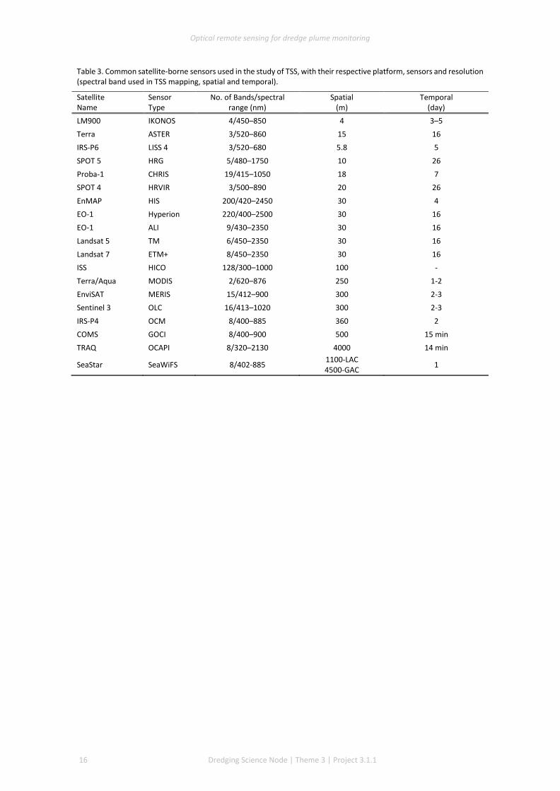
Table 3. Common satellite-borne sensors used in the study of TSS, with their respective platform, sensors and resolution (spectral band used in TSS mapping, spatial and temporal).

Satellite Name

Sensor Type

No. of Bands/spectral range (nm)

Spatial (m)

Temporal (day)

LM900 IKONOS 4/450–850 4 3–5 Terra ASTER 3/520–860 15 16 IRS-P6 LISS 4 3/520–680 5.8 5

SPOT 5 HRG 5/480–1750 10 26 Proba-1 CHRIS 19/415–1050 18 7 SPOT 4 HRVIR 3/500–890 20 26

EnMAP HIS 200/420–2450 30 4 EO-1 Hyperion 220/400–2500 30 16 EO-1 ALI 9/430–2350 30 16

Landsat 5 TM 6/450–2350 30 16 Landsat 7 ETM+ 8/450–2350 30 16 ISS HICO 128/300–1000 100 -

Terra/Aqua MODIS 2/620–876 250 1-2 EnviSAT MERIS 15/412–900 300 2-3 Sentinel 3 OLC 16/413–1020 300 2-3

IRS-P4 OCM 8/400–885 360 2 COMS GOCI 8/400–900 500 15 min TRAQ OCAPI 8/320–2130 4000 14 min

SeaStar SeaWiFS 8/402-885 1100-LAC 4500-GAC 1



3.2 Approaches used in TSS mapping

Ocean bio-geophysical parameters of interest are derived from remotely-sensed data, through quantitative empirical or semi-empirical and analytical methods. In remote sensing, the ‘base level’ information sensed by the sensors is radiance. This is usually converted to ocean reflectance which is then incorporated into an algorithm to derive products such as chlorophyll concentration, TSS or KPAR.

The Empirical method involves directly relating the remotely sensed data with in situ measurements or modelled parameters of interest using statistical analysis (linear and nonlinear regression).

Table 4. Satellites/sensors used in TSS mapping.

Satellites/sensors Features TSS mapping applications

Landsat TM

Medium to coarse spatial resolution with multispectral data (120 m for thermal infrared band and 30 m for multispectral bands) from Landsat 4 and 5 (1982 to present). Each scene covers an area of 170 × 185 km. Temporal resolution is 16 d.

Poor signal to noise and calibration.

Landsat ETM+(Landsat 7)

Medium to coarse spatial resolution with multispectral data (15 m for panchromatic band, 60 m for thermal infrared and 30 m for multispectral bands) (1999 to present). Each scene covers an area of 170 km × 185 km. Temporal resolution is 16 d.

Poor signal to noise and calibration, but Landsat 8 is improved.

SPOT

A full range of medium spatial resolutions from 20 m down to 2.5 m, and SPOT VGT with coarse spatial resolution of 1 km. Each scene covers 60 x 60 km for HRV/HRVIR/HRG and 1000 × 1000 km (or 2000 × 2000 km) for VGT. SPOT 1, 2, 3, 4 and 5 were launched in the years of 1986, 1990, 1993, 1998 and 2002, respectively. SPOT 1 and 3 are not providing data now.

Coarse spectral resolution but good spatial resolution.

MODIS

Low spatial resolution (250–1000 m) and multispectral data from the Terra Satellite (2000 to present) and Aqua Satellite (2002 to present). Revisit interval is around 1–2 d. Suitable for vegetation mapping at a large scale. The swath is 2330 km (cross track) by 10 km (along track at nadir).

Suited to dark targets (water) and able to provide daily views at 250 m resolution, etc.).

AVHRR 1-km GSD with multispectral data from the NOAA satellite series (1980 to present). The approximate scene size is 2400 × 6400 km

Historical coverage, poor spatial resolution.

IKONOS

It collects high-resolution imagery at 1 m (panchromatic) and 4 m (multispectral bands, including red, green, blue and near infrared) resolution. The revisit rate is 3–5 days (off-nadir). The single scene is 11 × 11 km.

High resolution.

QuickBird

High resolution (2.4–0.6 m) and panchromatic and multispectral imagery from a constellation of spacecraft. Single scene area is 16.5 × 16.5 km. Revisit frequency is around 1–3.5 d depending on latitude.

High resolution. Good but expensive.

ASTER

Medium spatial resolution (15–90 m) image with 14 spectral bands from the Terra Satellite (2000 to present). Visible to near-infrared bands have a spatial resolution of 15 m, 30 m for short wave infrared bands and 90 m for thermal infrared bands.

Free data.

AVIRIS

Airborne sensor collecting images with 224 spectral bands from visible, near infrared to short wave infrared. Depending on the satellite platforms and latitude of data collected, the spatial resolution ranges from meters to dozens of meters and the swath ranges from several kilometres to dozens of kilometres.

Expensive.

Hyperion Collects hyperspectral image with 220 bands ranging from visible to short wave infrared. The spatial resolution is 30 m. Data available since 2003.

Noisy.



Most empirical relationships take the following form:

𝑌𝑌 = 𝐴𝐴𝑥𝑥 + 𝐵𝐵 (14.)

𝑙𝑙𝑙𝑙𝑌𝑌 = 𝐴𝐴 + 𝐵𝐵𝑥𝑥 (15.)

where:

𝑥𝑥 is a measurement obtained using remote sensors;

Y is the parameter of interest; and

A and B are empirical factors.

Specifically, 𝑥𝑥 represents measurements of reflectance in a single spectral band (Tyler et al. 2006, Wang et al. 2008, Wu et al. 2008) or combination of bands (Kallio et al. 2008b, Kratzer et al. 2008, Duan et al. 2009) from respective remote sensing sensors.

From radiative transfer theory or modelling using Hydrolight, it can be established that reflectance is linearly dependent on TSS for relatively small concentrations, but as the concentration of TSS increases, linearity weakens, as the reflectance is affected by the contribution from absorption of TSS (Mobley 1994). In the case of high concentrations of TSS, a non-linear approximation is used to quantify TSS using higher order polynomials (Petus et al. 2010, Lim et al. 2013) and exponentials (Doxaran et al. 2003, Doxaran et al. 2006). The advantage of the empirical model over the semi-empirical or analytical models lies in its simplicity and computational efficiency in processing large volumes of data.

The semi-analytical or analytical methods involve relating the measured or modelled IOP of water to apparent optical properties – the irradiance reflectance just beneath the water surface to the concentration of constituents – to derive the parameter of interest through inversion techniques. For instance, the fundamental bio-optical model for turbid inland water according to Brando and Dekker (2003) takes the form:

𝑅𝑅(0 −)(𝜆𝜆) = 𝑓𝑓 ∗ 𝑏𝑏𝑏𝑏(𝜆𝜆)𝑎𝑎(𝜆𝜆)+𝑏𝑏𝑏𝑏(𝜆𝜆)

(16.)

where:

R(0-) is the sub-surface irradiance reflectance;

bb(λ) is the total backscattering coefficient of all water constituents;

a(λ) is the total absorption coefficient of all water constituents; and

f is a factor that accounts for anisotropy of the downwelling light field in water.

An extensive review of empirical procedures of remote sensing inland and near-coastal waters was presented by Matthews (2011). Appendix 1 reproduces a table based on the work of Matthews (2011) showing the form of remote sensing algorithms for a number of common space-borne sensors. It is interesting to note that the majority of the algorithms listed in Appendix 1 were published in the last 10 years, and none prior to 2000. The science is new and evolving.

A new development appearing in a range of environmental remote sensing applications is the multi-sensor and the multi-product approach. For example, Tatman et al. (2007) present a dredging information system (DIS) with features designed to visualise plume monitoring. They present what they term a method for synoptic monitoring of turbidity, which they represent as TSS. Remote sensing data from SeaWiFS, MODIS, Landsat and IKONOS are combined with in situ data and model simulations to determine background TSS levels. They use Delft-3D WAQ to model the transport and concentration of dredge related plumes. Short term model predictions are improved by including in situ and remote sensing data. Tatman et al. (2007) suggest that as the coverage of high resolution satellites improves, their DIS will be useful for operational monitoring of dredge plumes.



Vanhellemont and Ruddick (2014) describe the use of primarily MODIS and Landsat 8 OLI for the detection of turbine wakes. It does this using simple RGB imagery and a TSM product. They discuss how useful a number of sensors are for marine remote sensing based on the signal to noise ratio for bands near visible red in the spectrum. The MODIS ocean colour band 13 has the highest SNR followed by OLI band 4 then MODIS band 1. As MODIS band 1 is used for TSM or TSS retrievals, this makes OLI band 4 a good prospect. It shows a SPM and compares the results of OLI and MODIS. This paper also includes the atmospheric correction scheme used for OLI (Note: the aerosol correction uses the equivalent spectrum approach but does state it doesn’t hold true for highly turbid waters).

Chen et al. (2011) report on the monitoring of sediment plumes following large rainfall events. The sediment plume(s) were monitored by TSS estimates from MODIS data. The TSS estimates were determined from a model that used MODIS bands 1 and 2 Rrs data (red and near infrared respectively). A second order polynomial fit to a log/log plot of the band ratios against the in situ TSS produces a good r2 value, and reveals the locally tuned model.

The vertical distribution of in-water constituents can vary, thus the effect on the remotely sensed signal due to near-surface plumes, deep maxima or well mixed water columns is of interest, as well as the depth to which a satellite-borne sensor “sees” into the ocean. The remotely sensed reflectance is essentially an integral of the reflectance from all scattering layers in the ocean with the signal strength diminishing with increasing depth. The penetration depth of light, Z90, is defined as the depth above which 90% of the diffusely reflected irradiance originates (Gordon 1975), thus K may be used to estimate the depth over which a sensor can retrieve TSS estimates. Figure 2 shows K data for the clearest natural sea water from 200 nm to 800 nm, as well as the Z90 depth, estimated by 1/K. Notwithstanding the fact that K is a spectral quality, and IOP’s of in-water constituents exhibit spatiotemporal variability, we may consider as an example the depth of penetration for MODIS band 1 (620-680 nm), indicated in Figure 2 as a red highlight on the 1/K curve. In this case the depth of penetration is less than 5 m. As turbidity increases the depth of penetration would decrease. Another perspective to aid in the simple estimation of how far a satellite can “see” into the ocean is provided by reference to secchi depth measurements. Lee et al.(2015) discuss the relationship between the spectral diffuse attenuation coefficients of the water column with reference to visual perception of a secchi disc. Although the relationship is not precise, in simple terms the secchi depth is approximately equal to 1/K, and as noted in Section 2.2.8, this is also a reasonable estimate for the depth from which 90% of the light detected by an above water sensor originates.

Light from the substrate can impact the accuracy of a remotely sensed product if not accounted for. The science of shallow water remote sensing is reasonably well understood, relying on multi or hyperspectral measurements to simultaneously determine parameters such as water depth, substrate classification and water column constituent concentrations (Lee et al. 1999, Dekker et al. 2011). The algorithms listed in Appendix 1 are mainly based on either one or two spectral bands, thus are not designed to account for shallow water effects.

The remotely retrieved TSS is considered an average value for the depth of observation. Although there have been demonstrations of the potential to derive estimates of TSS vertical distribution, the results are limited and highly dependent on the actual water optical condition. Improvements to retrievals of TSS vertical structure may be improved by assimilation of data such as specific IOPs, field sampling and outputs from hydrologic models (Pitarch et al. 2014).



Figure 2. Attenuation coefficient of the clearest natural sea water and 1/K, an estimate of the depth of penetration (Z90). The depth of penetration for MODIS band 1 is indicated in red. K data are from Smith and Baker (1981).

3.3 Utilising in situ measurements to develop algorithms

In situ measurements can be used to establish relationships between Rrs and in-water parameters such as TSS, KPAR, or NTU. The DALEC may be used to collect Rrs data concurrently with collection of in-water parameters. The relationships derived from these data sets should be applicable to remote sensing data collected by airborne or space-borne sensors. Using the DALEC to collect the Rrs data avoids the need to consider atmospheric correction. Also, there is more control over the collection of concurrent data, as opposed to collection of in situ data during a satellite overpass. The real power of establishing these relationships is achieved when the relationships can be applied to satellite data. Establishing such a relationship allows the construction of maps. Where archives of satellite data exist, these relationships allow construction of an archive of a bio-geophysical parameter backwards in time, and extending into the future as more data are collected.

Time-series analysis of the bio-geophysical parameters can establish background conditions, trends and ‘hot spots’.

3.4 Remote Sensing Reflectance and TSS

To develop a TSS algorithm, Rrs is measured (using instruments such as the DALEC, Figure 1) whilst taking concurrent and collocated measurements of TSS through the sampling and filtering of water. The concurrent measurements are then fitted to a predefined equation to derive coefficients that represents a ‘local’ algorithm. Equation 17 (Evans et al., 2012) is an example of one of the many equations that are used to derive TSS (See Appendix 1).



𝑇𝑇𝑇𝑇𝑇𝑇 = 1𝑐𝑐1 𝑎𝑎𝑤𝑤𝑅𝑅𝑟𝑟𝑠𝑠(𝐵𝐵1)𝑐𝑐0−𝑅𝑅𝑟𝑟𝑠𝑠(𝐵𝐵1) − 𝑏𝑏𝑏𝑏𝑏𝑏 − 𝑐𝑐2 (17.)

where:

aw is the attenuation coefficient of pure water; and

bbw is the backscattering coefficient of pure water, and

c0, c1, c2 are coefficients determined by fitting the collocated data.

As Rrs can be retrieved from satellite data, equation 17 represents a method to produce TSS maps from remote sensing data.

Figure 3A is a satellite image of the Wheatstone dredging project near Onslow, in the Pilbara region of north-west Australia, captured on 23 May 2014 showing the dredge material placement site located east of Thevenard Island, dredging of a channel and flooding of the Ashburton River. Figure 3 B and C show two TSS maps derived from an algorithm similar to equation 20 where the coefficients are generic and not necessarily ‘tuned’ for this region. In situ data collected during Project 2/3 field activities could be used to refine the form of the algorithm and derive coefficient applicable to these waters. MODIS data (Figure 3B) are routinely used to produce TSS data. The Landsat 8 sensor provides higher spatial resolution data (Figure 3C), 30 m, compared to the 250 m data of MODIS. However, Landsat data are only available every 16 days whereas MODIS data are available daily. Landsat data are not routinely atmospherically corrected and are not optimized for ocean studies. An important aspect to highlight is the difference in the range of TSS values derived from the two sensors. The MODIS image shows maximum values at approximately 20 mg L-1 and Landsat 8 shows maxima at approximately 100 mg L-1.



A

B

C

Figure 3. Satellite images of the Wheatstone dredging project in the Pilbara region of north-west Australia on 23 May 2014 from (a) True colour image based on data from the United States Geological Survey (USGS) operational land imager (OLI) on Landsat 8, (b) MODIS Aqua derived TSS map and (c) Landsat 8 derived TSS map. The images show the dredge material placement site located east of Thevenard Island, dredging of a channel and flooding of the Ashburton River. The TSS maps are derived using a generic set of algorithms thus the TSS values are indicative only.



4 Available data

This section provides a brief overview of data sets that have been identified and made available and that may be useful for model development, model testing, algorithm development and validation. Due to restriction and embargoes not all of these data have yet been made available to RSSRG (Curtin University). Where data have not been made available to RSSRG, a summary of the data listings have been provided. These data are separated into in situ instrument data, remote sensing data and other data. Where possible, the potential uses of these data are identified, with a focus on the two main geophysical parameters that are most useful to describe the environmental impact of dredge plumes, sedimentation and light attenuation.

Table 5 provides an outline of data that have been made available to the WAMSI Dredge Science Node. Curtin University was provided with a listing of directories and files. The list below identifies possible data that will be useful to Theme 3, specifically the optical in situ and remotely sensed data. This list shows that there are many benthic data available, which may be of limited use for Theme 3. It also identifies acoustic data, which may be of use to the oceanographers of Theme 3, and potentially information on TSS and vertical structure of plumes. The acoustic data, which is able to map sediment plumes, may prove very useful if combined with optical data for mapping plumes.

Table 5. An outline of data collected during dredging projects in the NW Australia that have been made available to the WAMSI Dredging Science Node for scientific study.

Onslow, NW Australia

In situ instrumentation

For Stations at : Ashburton Island, Bessieres Island, Channel, Direction Island, Dredge route, Jetty, Offshore, Paroo Shoal, Platform, Serrurier Island, Spoil ground, Taunton reef, Thevenard Island, West Thevenard Island, Ward reef, Weeks Shoal, West Airlie, West Thevenard. Data captured for each site:

PAR Turbidity (Likely to be NTU) CTD ADCP (Acoustic Doppler Current Profiler) LISST AWAC (Acoustic Wave Current Profiler) Sonde DWR

Remote sensing None

Other

Seagrass video (towed) Biomass pictures Filter feeder pictures Macroalgae pictures 1000’s of photos for all of the sites and some video Processed data (WAMSI data transfer Q1 2014 – content of this directory is unknown) Near shore bathymetry

Barrow Island, NW Australia In situ instrumentation

Logger data (possibly temp) Excel files for water quality (Temp, sedimentation)

Remote sensing MODIS maps for Benthic Light Availability, Diffuse attenuation coefficient (PAR), true-colour images and Total Suspended Sediment (BLA, KdPAR, RGB and TSS)

Other Coral Health and water quality reports (pre-dredge) Lots of images (benthic)

Dampier, NW Australia


LISST data Temperature and turbidity reports Water quality reports

Remote sensing None Other Coral health survey reports James Price Point, NW Australia


Report on NTU TSS Kd relationship Reports on water quality Reports on sedimentation

Remote sensing Report on MODIS calibration (probably IMO local MODIS TSS algorithm)

Other Reports on benthos



The following data (Table 6) have been made available or were previously collected by RSSRG, Curtin University. These data are on storage systems that RSSRG can access and thus can be processed and analysed. The following list provides a more detailed listing/analysis of the available data than the previous section. These data are primarily from optical instruments (and gravimetric retrieval of TSS) but there are reports on coral health and sedimentation that are of limited use to project 2/3.

Table 6. An outline of data made available or were previously collected by RSSRG (Curtin University) for projects in the NW Australia (see text above).

Cape Lambert Port B project

4.1.1.1 In situ instrumentation

Sedimentation • The sedimentation is determined using sediment traps. This has been done both

pre, during and post dredge. There were a total of 57 deployments for 15 sites. Traps were deployed from late May 2010 to early November 2012. Deployments were typically between 1 and 3 weeks.

• Excel spreadsheet reporting gross sedimentation rate (mg/cm3/d). Deployment dates and sampling duration are also included

In Situ Marine Optics reports • There are 2 reports by In-situ Marine Optics, MODIS Algorithm Development and

development.pdf, CLPB_Verification_Report_RevB.pdf • The first of these is titled ‘MODIS Algorithm Development and Sedimentation

Transport Model Validation: Field Data Collection Report’. This report details the collection of Rrs, TSS, PAR, NTU, and Particle Size Distribution (PSD). These measurements were obtained using the DALEC, water sampling, Wetlabs ECO-PAR, Wetlabs ECO-NTU and LISST respectively. This report discusses the uses of the in situ data to develop algorithms for TSS retrieval from MODIS, as well as relationships between TSS and KdPAR, and TSS and NTU.

• The second report titled ‘Sediment Transport Model Verification’ details the use of TSS, NTU and MODIS TSS products to verify the Global Environmental Modelling System (GEMS) ability to estimate dredge plume extent.

NTUPAR • Contains 51 files with data in 3 – 5 columns. First 2 columns contain date and time.

Other columns have integer values. The units for the data columns is not evident. LISST

• 4 directories (FLOW, FULL, PRM, FULLFLOW) • These contain file types .psd, .log, .asc. The .log and .asc contain readable ascii

data. The data format, units and parameters are not evident in the file. SAV

• Contains IDL .sav files. These are data structures, which can contain a number of datasets in various formats. These can be read and output to other formats using IDL. Entries contain metadata entries for date, time, location etc. There are datasets for LISST transects, Remote sensing reflectance from the DALEC resampled to MODIS band 1 (645 nm) and PAR (not sure how this is derived) for 5 days of the deployment.

Remote Sensing Data

CLPB_MODIS_Composite_Imagery_RevB.pdf This report entitled ‘MODIS Composite Imagery during Dredging ‘describes methods for production of composite TSS products. These products include the average TSS over the period 23 Dec, 2010 – 18 Sep, 2012. This also includes images of the statistics associated with the average.

Other

Coral Spawning • Reports on coral spawning at different times of the year • Data consist of an Excel file for sites, dates and presence of coral spawning biota in

collected samples. Coral Health and Water Quality

• Monthly report on Water quality and a final report • Raw data in Excel files for Sedimentation, PSD, Turbidity, Temperature and PAR. • Processed data in Excel files for Temperature, NTU and PAR • Monthly report on coral health issues and a final report • Processed data in Excel files for coral health



Cape Lambert Port A


In-situ Marine Optics produced the following data. These data are summarised in various Word and Excel files, which are not explicitly mentioned below. Rrs: There are 64 files in binary format. . These are most likely DALEC files with hyperspectral Rrs values. There are several files for each file heading of site, transect, plume, dark plume and dark. There is a single file for Spectralon. These files are almost certainly DALEC files as this instrument is built and operated by IMO. These files are stored in a binary format where the normal ascii (human readable) format is compressed into an unstructured format. IMO have code to read these data. HR: This contains Hydrorad files where the filenames are likely to contain the date as part of the file number such as YYMMDD. Files exist for both A and B (downwelling and upwelling) channels. This instrument is likely to be the unit that belongs to RSSRG. These data can be processed with OEM software and specific calibration files, which RSSRG possesses. 7 daily files for both A and B channels and 2 daily files for the A channel only. NTU: There are 79 files for a number of sites, all in comma separated variable format. Measurements were taken with a Troll 9500 Professional XP meter (http://www.in-situ.com/rentals/water-quality/troll-9500-instrument). This measures temperature, salinity (conductivity), pH, dissolved Oxygen, Barometric pressure, NTU and depth. Not all readings are taken at all of the sites. C660: These data are in sub directories for Trip 1 and Trip 2. Trip 1 contains sub directories for days 1 – 8, trip appears to have been for 5 days. Each day sub directory contains text files which are labelled with the start letter A – G. A, B, contain columns for date, time, channel (either A or B) and 9 columns or data. E contains 3 columns of data. F and G appear to be NMEA of some other type of ascii output from a GPS. C660 is reported in the data summaries as attenuation coefficient at 660nm. There is a good chance that attenuation was recorded using the RSSRG C-Star instrument. This is normally output as RS232 in a single column of numbers. Once again clarification would need to be sort from IMO on the format of the data.

Remote sensing None

Other None Onslow, NW Australia


Liquid Robotics operated 2 wave gliders around the Thevenard island area in the periods Deember 2012–January 2013 and October 2013. One glider was deployed with a C-STAR transmissometer, ECO-puck, CTD and an ADCP. The other was deployed with a LISST. These gliders were able to autonomously circumnavigate their way on a set course around the Island. The C-STAR collects attenuation data as describe within this report and the ECO-puck records backscatter at 650 nm, 720 nm and 780 nm. RSSRG as part of a small proof of concept project in conjunction with the Centre for Marine Science and Technology, Curtin University, processed and evaluated the data captured during the deployment. The availability of these data for public use is not known at this time.

Remote sensing None

Other data None

Barrow Island, NW Australia


In August 2011 RSSRG in conjunction with the Department of Environment (DEC) and Conservation, now known as the Department of Parks and Wildlife (DPaW) captured surface radiometry data (Rrs) from the DALEC (2832 spectra) and collected water samples from 13 stations. These data were used to develop a local TSS model so that DEC could test the hand digitising method they developed to map dredge plumes. This work is described in detail in Evans et al., (2012).

Remote sensing None

Other None

5 Discussion

Remote sensing of dredging operations can provide a broad overview of the dredge affected areas and is the only available technology that can provide complete daily coverage over these areas. There are many satellite-derived algorithms that produce geophysical products (See Appendix 1), which can be used to monitor and manage dredge operations. The most valuable of these geophysical products provide information on the water quality such as sediment concentration and light attenuation. In order to develop these algorithms and then to

http://www.in-situ.com/rentals/water-quality/troll-9500-instrument

http://www.in-situ.com/rentals/water-quality/troll-9500-instrument



have confidence in the operation of these algorithms in situ data are required.

Perhaps the most useful satellite-derived products to monitor dredge plumes are those that provide estimates of suspended matter (i.e. TSS) and attenuation (i.e. Kd490, KPAR). Globally-based models can be used to determine these products but these can be prone to very large errors, especially in turbid coastal waters (Tassan, 1994, Lee et al., 2005). In order to produce reasonable estimates from satellite-derived data, local data are required to fit generic algorithms to local conditions.

Above water radiometry (Rrs) and water sample data are essential to develop locally tuned TSS algorithms. Based on the data listings and the data provided to RSSRG, TSS information is available as data or in reports for the projects at: Barrow Island (Gorgon LNG), Onslow (Wheatstone LNG), James Price Point (Browse LNG) and Cape Lambert (A and B ports). Rrs information is available either within reports or as data at: Onslow, Barrow Island, James Price Point and Cape Lambert (A and B ports).

A potential advantage of these datasets is the likelihood that these data were captured with the same type of instrument (DALEC) and TSS methods as outlined earlier. This compatibility of datasets may allow investigation into development of robust algorithms that operate more effectively across different water types without the need to collect in situ data to train the algorithm.

Hydrorad or similar irradiance measurements within the water column give definitive measurements of the spectral nature of the available light at depth. The two major impact pathways by which dredging affects benthic communities are considered to be suffocation by deposited sediment and the reduction of light due to attenuation within the sediment plume. The Hydrorad can be used to derive diffuse attenuation coefficients such as Kd490. Diffuse attenuation maps derived from satellite data from local algorithms can be converted to benthic light availability maps, where bathymetry data are available. This provides information on one of the main impacts of dredging. PAR sensors measure the light at depth. As described in Section 2.2.6, this single broadband irradiance measurement may not accurately reflect the useful light available at the benthic level. PAR sensors can be used to measure light at different depths in the water column and a light attenuation coefficient (KPAR), or the diffuse attenuation from 400–700 nm, can be derived from these data. This requires that the PAR sensor is used to profile or that the PAR sensor is matched to a sensor at a different depth or just above the surface of the water. These data can be used to verify satellite-derived KPAR data. PAR data are available from the sites: Onslow, James Price Point and Cape Lambert port B. Hydrorad data was captured at Onslow and Cape Lambert port A.

The attenuation of light in the water column correlates strongly with the suspended sediment concentration (Devlin et al. 2008). Devlin et al. (2008) describe that fitting separate relationships to waters from offshore, coastal and transitional (estuarine) zones produces better results than simply fitting to all gathered data. It does not touch on the effect of different sediment types on these relationships. Given that there are data available that have been collected in the same manner, and for at least for 2 projects hyperspectral data have been captured, this provides an opportunity to study how sediment composition and the TSS to K relationships inter-relate.

The ac-s, C-STAR, Hydroscat and LISST derive inherent optical properties of absorption (a), scattering (b) and attenuation (c) and particle size/concentration information in the marine environment. These IOPs are the crucial inputs into radiative transfer models such as Hydrolight and are used in many algorithms to derive products, such as the semi-empirical diffuse attenuation algorithm described in Lee et al. (2005).

The ac-s and Hydroscat instruments, and instrument like these, produce beam scattering and backscattering information. Scattering and specifically backscattering correlate strongly to Rrs as it is this scattered signal that is received by above-water radiometers and satellite instruments. It is possible to produce quantifiable relationships between Rrs and the beam scattering coefficient and if this relationship is applied to satellite-derived Rrs then maps of the scattering coefficients can be produced. If the absorption from the ac-s is subjected to the same set of steps then it is also potentially possible to produce maps of this as well. As IOPs are used as inputs to many algorithms that produce biophysical products (Lee et al., 2005) these maps can be used as input



to many algorithms.

Data from the LISST can be used to infer particle size distribution. PSD is of primary importance to oceanographic modellers as this will inform on settling rates and plume dispersal. It is perhaps of less importance to optical modelling and derivation of biophysical parameters. PSD does affect the amount of scattering and thus the IOPs of the water body but this information is already captured using instruments such as the ac-s and Hydroscat.

Criteria to trigger management actions in dredge management plans are often expressed in terms of NTU as this is the most commonly used parameter to monitor turbidity using in-situ sensors and in near real-time. NTU measurements by themselves do not adequately describe the potential effects of sediment loading. If relationships between NTU and TSS or NTU and PAR are established for local conditions then NTU data can be of greater benefit as they would allow determination of these more useful measurements. The NTU data converted to TSS could also prove useful for the validation of satellite-derived TSS products.

6 Conclusions

It has been well demonstrated that in situ data form an integral part in the design and development of remote sensing algorithms that require ‘local tuning’. As requirements to monitor dredging operations become more common, more and varied data are being collected. Combining surface and sub-surface in situ measurements allows the complex interactions of light within a dynamically variable water body to be better understood and for useful biophysical products to be derived from a limited set of observations. When these relationships are applied to satellite-retrieved data, monitoring of dredge operations can be undertaken over large areas and on a sub-daily temporal basis.

With more ‘local’ data becoming available it is possible to investigate how the constituents of the water bodies influence the relationships introduced in this review with the aim to produce a simplified set of measurements and steps to effectively provide environmental monitoring of future dredging operations.



7 References

Acker JG, Harding LW, Leptoukh G, Zhu T, Shen S (2005) Remotely-sensed chl a at the Chesapeake Bay mouth is correlated with annual freshwater flow to Chesapeake Bay. Geophys Res Lett 32:L05601

Alparslan E, Aydöner C, Tufekci V, Tüfekci H (2007) Water quality assessment at Ömerli Dam using remote sensing techniques. Environ Monit Assess 135:391-398

Anthony K, Ridd P, Orpin A, Larcombe P, Lough J, (2004), ‘Temporal variations of light availability in coastal benthic habitats: Effects of clouds, turbidity, and tides’, Limnol Oceanogr, 49:2201 - 2211

Ammenberg P, Flink P, Lindell T, Pierson D, Strombeck N (2002) Bio-optical modelling combined with remote sensing to assess water quality. Int J Remote Sens 23:1621-1638

Arrigo KR, McClain CR (1994) Spring Phytoplankton Production in Western Ross Sea. Science 266:261-263

Asadpour R, Lim HS, Alashoo MM, Mousavi SY (2012) A statistical model for mapping spatial distribution of total suspended solid from THEOS satellite imagery over Penang Island, Malaysia.J Appl Sci Res 8:271-276

Barnes C, Tibbitts T, Sager J, Deitzer G, Bubenheim D, Koerner G, and Bugbee B (1993) Accuracy of Quantum Sensors Measuring Yield Photon Flux and Photosynthetic Photon Flux, HortScience 28(12):1197–1200

Binding CE, Bowers DG, Mitchelson-Jacob EG (2003) An algorithm for the retrieval of suspended sediment concentrations in the Irish Sea from SeaWiFS ocean colour satellite imagery. Int J Remote Sens 24:3791-3806

Binding CE, Bowers DG, Mitchelson-Jacob EG (2005) Estimating suspended sediment concentrations from ocean colour measurements in moderately turbid waters; the impact of variable particle scattering properties. Remote Sens Environ 94:373-383

Bortones SA (2000) Seagrasses: monitoring, ecology, physiology, and management. CRC Press

Brando VE, Dekker AG (2003) Satellite hyperspectral remote sensing for estimating estuarine and coastal water quality. IEEE T Geosci Remote 41:1378-1387

Brezonik P, Menken KD, Bauer M (2005) Landsat-based Remote Sensing of Lake Water Quality Characteristics, Including Chlorophyll and Colored Dissolved Organic Matter (CDOM). Lake Reserv Manage 21:373-382

Bukata, R.P., Jerome, J.H., Kondratyev, K.Y. and Pozdnyakov, D.V., (1995) "Optical properties and remote sensing of inland and coastal waters", Publisher, CRC Press, Inc., Florida, 362 pp.

Cai W, Yuan W, Liang S, Zhang X, Dong W, Xia J, Fu Y, Chen Y, Liu D, Zhang Q (2014) Improved estimations of gross primary production using satellite-derived

photosynthetically active radiation. J Geophys Res-Biogeosci 119:2013JG002456

Chen Z, Hu C, Muller-Karger F (2007) Monitoring turbidity in Tampa Bay using MODIS/Aqua 250-m imagery. Remote Sens Environ 109:207-220

Chen, S., Huang, W., Chen, W., Chen, X., (2011), ‘An enhanced MODIS remote sensing model for detecting rainfall effects on sediment plume in the coastal waters of Apalachicola Bay’, Mar Environ Res, 72: 265 – 272

Chen J, D'Sa E, Cui T, Zhang X (2013) A semi-analytical total suspended sediment retrieval model in turbid coastal waters: A case study in Changjiang River Estuary. Opt Express 21:13018-13031

Chen J, Cui T, Qiu Z, Lin C (2014a) A three-band semi-analytical model for deriving total suspended sediment concentration from HJ-1A/CCD data in turbid coastal waters. ISPRS J Photgramm 93:1-13

Chen J, Cui T, Tang J, Song Q (2014b) Remote sensing of diffuse attenuation coefficient using MODIS imagery of turbid coastal waters: A case study in Bohai Sea. Remote Sens Environ 140:78-93

Clarke, D., Wilber, D., (2008), ‘Compliance monitoring of dredge-induced turbidity: defective designs and potential solutions’, proceedings of the Western Dredging Association 28th technical conference.

Darbra RM, Ronza A, Casal J, Stojanovic TA, Wooldridge C (2004) The Self Diagnosis Method: A new methodology to assess environmental management in sea ports. Mar Pollut Bull 48:420-428

Dekker AG, Vos RJ, Peters SWM (2002) Analytical algorithms for lake water TSM estimation for retrospective analyses of TM and SPOT sensor data. Int J Remote Sens 23:15-35

Dekker AG, Phinn SR, Anstee J, Bissett P, Brando VE, Brando, Casey B, Fearns P, Hedley J, Klonowski W, Lee Z-P, Lynch M, Lyons M, Mobley C, Roelfsema C (2011) Intercomparison of shallow water bathymetry, hydro-optics, and benthos mapping techniques in Australian and Caribbean coastal environments, Limnol. Oceanogr. Methods 9, 396-425

Department of Water (2009), ‘Surface water sampling methods and analysis – technical appendices, Standard operating procedures for water sampling – methods and analysis’, retrieved from http://www.water.wa.gov.au/PublicationStore/first/87152.pdf Aug, 2014.

Devlin MJ, Barry J, Mills DK, Gowen RJ, Foden J, Sivyer D and Tett P (2008) Relationships between suspended particulate material, light attenuation and Secchi depth in UK marine waters. Estuar Coast Shelf S 79 (2008) 429–439

Downing J, (2006) ‘Twenty-five years with OBS sensors: The good, the bad and the ugly’, Cont Shelf Res, Vol. 26, 17:18, 1995-2018

http://www.water.wa.gov.au/PublicationStore/first/87152.pdf

http://www.water.wa.gov.au/PublicationStore/first/87152.pdf



Doxaran D, Castaing P, Lavender SJ (2006) Monitoring the maximum turbidity zone and detecting fine-scale turbidity features in the Gironde estuary using high spatial resolution satellite sensor (SPOT HRV, Landsat ETM+) data. Int J Remote Sens 27:2303-2321

Doxaran D, Froidefond J-M, Castaing P (2003) Remote-sensing reflectance of turbid sediment-dominated waters. Reduction of sediment type variations and changing illumination conditions effects by use of reflectance ratios. Appl Optics 42:2623-2634

Doxaran D, Froidefond J-M, Castaing P, Babin M (2009) Dynamics of the turbidity maximum zone in a macrotidal estuary (the Gironde, France): Observations from field and MODIS satellite data. Estuar Coast Shelf S 81:321-332

Doxaran D, Froidefond J-M, Lavender S, Castaing P (2002a) Spectral signature of highly turbid waters: Application with SPOT data to quantify suspended particulate matter concentrations. Remote Sens Environ 81:149-161

Doxaran D, Froidefond JM, Castaing P (2002b) A reflectance band ratio used to estimate suspended matter concentrations in sediment-dominated coastal waters. Int J Remote Sens 23:5079-5085

Duan H, Ma R, Zhang Y, Zhang B (2009) Remote-sensing assessment of regional inland lake water clarity in northeast China. Limnology 10:135-141

Ekercin S (2007) Water Quality Retrievals from High Resolution Ikonos Multispectral Imagery: A Case Study in Istanbul, Turkey. Water Air Soil Poll 183:239-251

EPA (1999) Total Suspended Solids (TSS) EPA Method 160.2. Revision 11/16/1999. https://www.epa.gov/sites/production/files/2015-06/documents/160_2.pdf

EPA (2016) Technical Guidance: Environmental Impact Assessment of Marine Dredging Proposals. Environmental Protection Authority, Western Australia.

Evans, D, Murray, K, Field, S, Moore, J, Huntley, B, Fearns, P, Broomhall, M, McKinna, L, Marrable, D (2012) Digitise This! A Quick and Easy Remote Sensing Method to Monitor the Daily Extent of Dredge Plumes. PLoS ONE 7(12)

Fettweis M, Nechad B, Van den Eynde D (2007) An estimate of the suspended particulate matter (SPM) transport in the southern North Sea using SeaWiFS images, in situ measurements and numerical model results. Cont Shelf Res 27:1568-1583

Fischer, J. and Grassl, H. (1984), Radiative transfer in an atmosphere-ocean system: an azimuthally dependent matrix-operator approach, Appl Optics, Vol. 23, No. 7, 1032-1039.

GBRMPA, 2012 GBRMPA (2012) Guidelines: The use of Hydrodynamic Numerical Modelling for Dredging Projects in the Great Barrier Reef Marine Park, Australian Government, Great Barrier Reef Marine Park Authority, August 2012.

http://www.gbrmpa.gov.au/__data/assets/pdf_file/0018/26532/Guidelines-on-Hydrodynamics-Modelling-15-Aug-2012.pdf

Giardino C, Brando VE, Dekker AG, Strömbeck N, Candiani G (2007) Assessment of water quality in Lake Garda (Italy) using Hyperion. Remote Sens Environ 109:183-195

Giardino C, Pepe M, Brivio PA, Ghezzi P, Zilioli E (2001) Detecting chlorophyll, Secchi disk depth and surface temperature in a sub-alpine lake using Landsat imagery. Sci Total Environ 268:19-29

Gordon, H.R. (1975), Computed relationships between the inherent and apparent optical properties of a flat homogeneous ocean, Appl Optics, Vol. 14, No. 2. 417-427

Gordon, H.R. and McCluney, W.R. (1975), Estimation of the depth of sunlight penetration in the sea for remote sensing, Appl Optics, Vol. 14, No. 2, 413-416

Hall MO, Tomasko DA, Courtney FX Response of Thalassia testudinum to in situ light reduction. In: Kenworthy WJ, Haunert DE (eds). Proc The Light Requirement of Seagrasses, NOAA Tech Memo

Härmä P, Vepsäläinen J, Hannonen T, Pyhälahti T, Kämäri J, Kallio K, Eloheimo K, Koponen S (2001) Detection of water quality using simulated satellite data and semi-empirical algorithms in Finland. Sci Total Environ 268:107-121

Hausknecht, P. (2010) Operational MODIS Satellite based water turbidity monitoring for dredging operations in Woodside, Woodside - GTO – Geomatics. OGP Remote Sensing workshop held at European Space Agency, Sept. 2010, DRIMS #5526810

Hellweger F, Miller W, Oshodi K (2007) Mapping Turbidity in the Charles River, Boston Using a High-resolution Satellite. Environ Monit Assess 132:311-320

Hellweger FL, Schlosser P, Lall U, Weissel JK (2004) Use of satellite imagery for water quality studies in New York Harbor. Estuar Coast Shelf S 61:437-448

Jutla AS, Akanda AS, Islam S (2012) Satellite remote sensing of space–time plankton variability in the Bay of Bengal: Connections to cholera outbreaks. Remote Sens Environ 123:196-206

Kallio K, Attila J, Härmä P, Koponen S, Pulliainen J, Hyytiäinen U-M, Pyhälahti T (2008a) Landsat ETM+ Images in the Estimation of Seasonal Lake Water Quality in Boreal River Basins. Environ Manage 42:511-522

Kallio K, Attila J, Harma P, Koponen S, Pulliainen J, Hyytianinen UM, Pyhalahti T (2008b) Landsat ETM+ Images in the estimation of seasonal lake water quality in boreal river basins. Environ Manage:511-522

Kallio K, Kutser T, Hannonen T, Koponen S, Pulliainen J, Vepsäläinen J, Pyhälahti T (2001) Retrieval of water quality from airborne imaging spectrometry of various lake types in different seasons. Sci Total Environ 268:59-77






Kirk, J.T.O. (1983), Light and Photosynthesis in Aquatic Ecosystems", Publisher, Cambridge University Press, Cambridge, 401 pp.

Kloiber SM, Brezonik PL, Olmanson LG, Bauer ME (2002) A procedure for regional lake water clarity assessment using Landsat multispectral data. Remote Sens Environ 82:38-47

Koponen S, Attila J, Pulliainen J, Kallio K, Pyhälahti T, Lindfors A, Rasmus K, Hallikainen M (2007) A case study of airborne and satellite remote sensing of a spring bloom event in the Gulf of Finland. Cont Shelf Res 27:228-244

Koponen S, Pulliainen J, Kallio K, Hallikainen M (2002) Lake water quality classification with airborne hyperspectral spectrometer and simulated MERIS data. Remote Sens Environ 79:51-59

Kratzer S, Brockmann C, Moore G (2008) Using MERIS full resolution data to monitor coastal waters — A case study from Himmerfjärden, a fjord-like bay in the northwestern Baltic Sea. Remote Sens Environ 112:2284-2300

Kutser T, Pierson DC, Tranvik L, Reinart A, Sobek S, Kallio K (2005) Using Satellite Remote Sensing to Estimate the Colored Dissolved Organic Matter Absorption Coefficient in Lakes. Ecosystems 8:709-720

Lee Z-P, Carder KL, Mobley CD, Steward RG, Patch JS (1999) Hyperspectral remote sensing for shallow waters: 2. Deriving bottom depths and water properties by optimization. Appl Optics 38

Lee Z-P, Du K-P and Arnone R (2005), A model for the diffuse attenuation coefficient of downwelling irradiance, J Geophys Res, 110, C02016, doi:10.1029/2004JC002275

Lee Z-P, Shang S, Hu C, Du K, Weidemann A, Hou W, Lin J and Lin G, (2015) Secchi disk depth: A new theory and mechanistic model for underwater visibility, Remote Sens Environ, Vol. 169, pp 139-149, ISSN 0034-4257, https://doi.org/10.1016/j.rse.2015.08.002.

Lee Z-P, Ahn Y, Mobley C, Arnone R, (2010), ‘Removal of surface-reflected light for the measurement of remote-sensing reflectance from an above-surface platform’, Opt Express, 18: 26313 – 26324

Li L, Xin X, Su G, Liu Q (2010) Photosynthetically active radiation retrieval based on HJ-1A/B satellite data. Sci China Earth Sci 53:81-91

Lim HS, MatJafri MZ, Abdullah K, Asadpour R (2013) A Two-Band Algorithm for Total Suspended Solid Concentration Mapping Using THEOS Data. J Coastal Res 29:624-630

Loisel H, Vantrepotte V, Dessailly D, MÈriaux X (2014) Assessment of the colored dissolved organic matter in coastal waters from ocean color remote sensing. Opt Express 22:13109-13124

McCook, LJ, Schaffelke, B, Apte, SC, Brinkman, R, Brodie, J, Erftemeijer, P, Eyre, B, Hoogerwerf, F, Irvine, I, Jones, R, King, B, marsh, H, Masini, R, morton, R, Pitcher, R, Rasheed, M, Sheaves, M, Symonds, A & Warne,

MSt.J (2015), Synthesis of current knowledge of the biophysical impacts of dredging and disposal on the Great Barrier Reef: report of an independent panel of experts, Great Barrier Reef Marine Park Authority, Townsville, Qld. ISBN: 9781922126573

Mabwoga SO, Chawla A, Thukral AK (2010) Assessment of water quality parameters of the Harike wetland in India, a Ramsar site, using IRS LISS IV satellite data. Environ Monit Assess 170:117-128

Martinez JM, Guyot JL, Filizola N, Sondag F (2009) Increase in suspended sediment discharge of the Amazon River assessed by monitoring network and satellite data. CATENA 79:257-264

Matthews MW (2011) A current review of empirical procedures of remote sensing in inland and near-coastal transitional waters, Int J Remote Sens Vol. 32 , Iss. 21, 6855-6899

Mueller JL, Brown SW, Clark DK, Johnson BC, Yoon H, Lykke KR,. Flora SJ, Feinholz ME, Souaidia N, Pietras C, Stone TC, Yarbrough MA, Kim YS and Barnes RA (2004) Ocean Optics Protocols For Satellite Ocean Color Sensor Validation, Revision 5, Volume VI: Special Topics in Ocean Optics Protocols, Part 2 Mueller JL, Fargion GS and McClain CR, (Eds.) NASA Goddard Space Flight Center, Greenbelt, MD, NASA/TM-2004-

Mills D, Kemps H (2016) Generation and release of sediments by hydraulic dredging: a review. Report of Theme 2 - Project 2.1 prepared for the Dredging Science Node, Western Australian Marine Science Institution, Perth, Western Australia. 97 pp.

Miller RL, McKee BA (2004) Using MODIS Terra 250 m imagery to map concentrations of total suspended matter in coastal waters. Remote Sens Environ 93:259-266

Mobley CD (1994) Light and Water: Radiative Transfer in Natural Waters. Academic San Diego, CA

Mobley, C, (1999), ‘Estimation of the remote-sensing reflectance from above-surface measurements’, Appl Optics, 38: 7442 – 7455

Mobley, C, (2010), ‘Overview of Optical Oceanography: Inherent Optical Properties’, Ocean Optics Web Book, retrieved Aug, 2014, http://www.oceanopticsbook.info/

Morel A and Gentili B (1993). Diffuse reflectance of oceanic waters. 2. Bidirectional aspects. Appl Optics, 32, 6864-6872.

Neukermans G, Ruddick K, Bernard E, Ramon D, Nechad B, Deschamps P-Y (2009) Mapping total suspended matter from geostationary satellites: a feasibility study with SEVIRI in the Southern North Sea. Opt Express 17:14029-14052

Odermatt D, Heege T, Nieke T, Kneubuhler M, Itten KI (2008) Water quality monitoring for Lake Constance with a physically based algorithm for MERIS data. Sensors 8:4582-4599

http://www.tandfonline.com/doi/abs/10.1080/01431161.2010.512947



http://www.tandfonline.com/toc/tres20/32/21



Olmanson LG, Bauer ME, Brezonik PL (2008) A 20-year Landsat water clarity census of Minnesota's 10,000 lakes. Remote Sens Environ 112:4086-4097

Omar, A., MatJafri, M., (2009), ‘Turbidimeter Design and Analysis: A Review on Optical Fiber Sensors for the Measurement of Water Turbidity’, Sensors, 9:8311 - 8335

Onderka M, Pekárová P (2008) Retrieval of suspended particulate matter concentrations in the Danube River from Landsat ETM data. Sci Total Environ 397:238-243

Östlund C, Flink P, Strömbeck N, Pierson D, Lindell T (2001) Mapping of the water quality of Lake Erken, Sweden, from Imaging Spectrometry and Landsat Thematic Mapper. Sci Total Environ 268:139-154

Ouillon S, Douillet P, Petrenko A, Neveux J, Dupouy C, Froidefond J-M, Andréfouët S, Muñoz-Caravaca A (2008) Optical Algorithms at Satellite Wavelengths for Total Suspended Matter in Tropical Coastal Waters. Sensors 8:4165-4185

Petus C, Chust G, Gohin F, Doxaran D, Froidefond J-M, Sagarminaga Y (2010) Estimating turbidity and total suspended matter in the Adour River plume (South Bay of Biscay) using MODIS 250-m imagery. Cont Shelf Res 30:379-392

Pitarch J, Odermatt D, Kawka M, and Wüest A (2014), Retrieval of vertical particle concentration profiles by optical remote sensing: a model study, Opt. Express 22, A947-A959 https://doi.org/10.1364/OE.22.00A947

Preisendorfer RW and Mobley CD (1984), Direct and inverse irradiance models in hydrologic optics, Limnol Oceanogr, Vol. 29, No. 5, 903-929.

Robinson AR (1971) Sediment: Our greatest pollutant. J Soil Water Conserv 53:406-408

Sabol B, Shafer D (2005), ‘Dredging effects on seagrass: Case studies from New England and Florida’, 25th Annual Western Dredging Association Conference.

Sadar M (1998) Turbidity Science, Technical Information Series – Booklet No. 11, Hach Company

Sawaya KE, Olmanson LG, Heinert NJ, Brezonik PL, Bauer ME (2003) Extending satellite remote sensing to local scales: land and water resource monitoring using high-resolution imagery. Remote Sens Environ 88:144-156

Smith RC and Baker KS (1981) Optical properties of the clearest natural waters (200–800 nm), Appl. Opt. 20, 177-184

Sofonia J, Unsworth R, (2010), ‘Development of water quality thresholds during dredging for the protection of benthic primary producer habitats’, J Environ Monitor, 12:159 - 163

Sridhar N, Ali MM, Rao MV, and Nagamani PV (2012) Photosynthetically active radiation, a critical parameter for mass coral bleaching in the North Indian Ocean, Curr Sci, Vol. 102, No. 1, 114-118

Standards Australia (1990) Waters. Part 4: Determination of solids - Gravimetric method (AS 3550.4 - 1990). Homebush, NSW: Standards Australia

Stone J (2003) Suspended Solids: Unequal results from equal methods. https://www.envexp.com/pdf/PWUnequal.pdf

Strickland JD and Parsons TR (1972) A practical handbook of seawater analysis. Bull. Fish. Res. Bd. Can. 167. 310 pp

Sudheer KP, Chaubey I, Garg V (2006) Lake water quality assessment from Landsat Thematic Mapper data using neural network: an approach to optimal band combination selection. J Am Water Resour As 42:1683-1695

Sullivan CW, Arrigo KR, McClain CR, Comiso JC, Firestone J (1993) Distribution of Phytoplankton Blooms in the Southern Ocean. Science 262:1832-1837

Sváb E, Tyler AN, Preston T, Présing M, Balogh KV (2005) Characterizing the spectral reflectance of algae in lake waters with high suspended sediment concentrations. Int J Remote Sens 26:919-928

Tang S, Larouche P, Niemi A, Michel C (2013) Regional algorithms for remote-sensing estimates of total suspended matter in the Beaufort Sea. Int J Remote Sens 34:6562-6576

Tassan S (1994) Local algorithms using SeaWiFS data for the retrieval of phytoplankton, pigments, suspended sediment, and yellow substance in coastal waters, Appl Opt 33, 2369-2378

Tatman S, Dirks W, Gerritsen H, Hesselmans G, Noorbergen H (2007) A new dredging information system (DIS) for assessment of environmental effects of tubidity, Proceedings of the Eighteenth World Dredging Congress (WODCON XVIII), May27 -June 1,2007, Lake Buena Vista, Florida, USA. World Organisation of Dredging Associations. Ed. RE Randall, Newman Print. Company, 1274 pp

Tiwari SP, Shanmugam P (2011) An optical model for the remote sensing of coloured dissolved organic matter in coastal/ocean waters. Estuar Coast Shelf S 93:396-402

Tyler AN, Svab E, Preston T, Présing M, Kovács WA (2006) Remote sensing of the water quality of shallow lakes: A mixture modelling approach to quantifying phytoplankton in water characterized by high-suspended sediment. Int J Remote Sens 27:1521-1537

US EPA, (2012), ‘Water: Monitoring and Assessment. 5.5 Turbidity’, US Environmental Protection Agency, Washington DC. http://water.epa.gov/type/rsl/monitoring/vms55.cfm, retrieved Aug, 2104

Vanhellemont, Q, Ruddick, K, (2014), ‘Turbid wakes associated with offshore wind turbines observed with Landsat 8’, Remote Sens Environ, 145: 105 – 115

Vincent RK, Qin X, McKay RML, Miner J, Czajkowski K, Savino J, Bridgeman T (2004) Phycocyanin detection

http://water.epa.gov/type/rsl/monitoring/vms55.cfm

http://water.epa.gov/type/rsl/monitoring/vms55.cfm



from LANDSAT TM data for mapping cyanobacterial blooms in Lake Erie. Remote Sens Environ 89:381-392

Vos RJ, Hakvoort JHM, Jordans RWJ, Ibelings BW (2003) Multiplatform optical monitoring of eutrophication in temporally and spatially variable lakes. Sci Total Environ 312:221-243

Wang F, Han L, Kung HT, Van Arsdale RB (2006) Applications of Landsat-5 TM imagery in assessing and mapping water quality in Reelfoot Lake, Tennessee. Int J Remote Sens 27:5269-5283

Wang F, Zhou B, Xu J, Song L, Wang X (2008) Application of neural netword and MODIS 250m imagery for estimating suspended sediments concentration in Hangzhou Bay, China. Environ Geol 56:1093-1101

Wang XJ, Ma T (2001) Application of Remote Sensing Techniques in Monitoring and Assessing the Water Quality of Taihu Lake. B Environ Contam Tox 67:863-870

Wetlabs, (2011), ‘Transmissometer C-Star User’s Guide’, Wetlabs, Inc., revision V, retrieved 13/08/2014, http://www.wetlabs.com/sites/default/files/documents/C-Star-Rev-V-Manual.pdf

Wu G, De Leeuw J, Skidmore AK, Prins HHT, Liu Y (2008) Comparison of MODIS and Landsat TM5 images for mapping tempo–spatial dynamics of Secchi disk depths in Poyang Lake National Nature Reserve, China. Int J Remote Sens 29:2183-2198

Wu M, Zhang W, Wang X, Luo D (2009) Application of MODIS satellite data in monitoring water quality parameters of Chaohu Lake in China. Environ Monit Assess 148:255-264

Zacher K (2014) The susceptibility of spores and propagules of Antarctic seaweeds to UV and photosynthetically active radiation — Field versus laboratory experiments. J Exp Mar Biol Ecol 458:57-63

Zhang Y, Pulliainen J, Koponen S, Hallikainen M (2002) Application of an empirical neural network to surface water quality estimation in the Gulf of Finland using combined optical data and microwave data. Remote Sens Environ 81:327-336

Zhou W, Wang S, Zhou Y, Troy A (2006) Mapping the concentrations of total suspended matter in Lake Taihu, China, using Landsat-5 TM data. Int J Remote Sens 27:1177-1191



8 Appendices

Appendix 1. The Table below is adapted from Matthews (2011) and shows the TSS algorithms and their characteristics for a number of sensors

Reference Location Data Type

Atmospheric Correction

Water Parameter

Data Range mg L-1

Statistical Technique Bands/Algorithms Regression

coefficient Error N L

TSS, TSM, SSC, SPM MODIS Petus et al. (2010)

Bay of Biscay, France MODIS MODIS level 2G TSS 0.3-145.6 2nd order

polynomial TSM = 12,450Rrs(B1)2 + 666.1Rrs(B1)

+ 0.4 r2 = 0.97 RMSE=61% 74 1

Doxaran et al. (2009)

Gironde Estuary, France MODIS Dark Pixel

Method SPM - Exponential SPM = 12.996e[Rrs(B2) Rrs(B1)]⁄

0.189 r2 = 0.89 Terra: 22% Aqua: 18% 204 2

Wang et al. (2008)

Hangzhou Bay, China MODIS 6S model SSC 0-2500 Log Transformed

Linear ln(SSC) = 50.171B1 − 1.523 ln(SSC) = 43.233B2 − 1.396

r2 = 0.73 r2 = 0.76

RMSE =501 RMSE=424 mg/l

25

Miller and McKee (2004)

Northern Gulf of Mexico, USA MODIS Dark-object

subtraction TSM 1-55 Linear TSM = 1140.25Rrs(B1) − 1.91 r2 = 0.89 RMSE=4.74 mg/l 52

LANDSAT Onderka and Pekárová (2008)

Danube River, Slovakia

Landsat 7 ETM+ - SPM 19.5-57.5 Linear SPM = 4.17L(TM4) − 43.22 r2 = 0.93 RMSE

3.2mg/l 10

Alparslan et al. (2007)

Omerli Dam, Turkey

Landsat 7 ETM+

Dark-object subtraction TSS 0.4-2.9 Multiple Linear

regression TSS = 42.2672 − 0.8694B1 − 0.3716B2 +1.05B3 + 0.1247B4 r2 = 0.99 RMSE

1% 6

Sudheer et al. (2006)

Beaver Reservoir, USA

Landsat TM - TSS 0-11.5 ANN Linear TM1, TM2. TM3, TM4 r2 = 0.98 2.02mg/l 25

Tyler et al. (2006)

Lake Balaton, Central Europe

Landsat TM

Dark-object subtraction TSS 5-50 Linear TSS = 1.36TM3 − 2.44 r2

= 0.891 - 22


Gironde Estuary, France

Landsat ETM+

6S, Dark-object subtraction TSS 10-2000 Exponential SPM = 29.0e0.0335∗Landsat[Rrs(L4) Rrs(L2)]⁄ r2 = 0.88 - 132

Wang et al. (2006)

Lake Reelfoot, USA

Landsat 5 TM Radiometric TSS 11.5-33.5 Multiple Linear TSS = 22.74 + 156.202M2 − 147.62TM3

− 45.66TM4 r2 = 0.52 - 18

Sváb et al. (2005)

Lake Balaton, Central Europe Landsat - TSS 2-40.5 Linear TM2/TM3 r2 = 0.94 10


Gironde Estuary, France Landsat - SPM 13-2388 Exponential SPM = 29.0e0.0335∗Landsat[Rrs(L4) Rrs(L2)]⁄ r2 = 0.88 - 132 3



Sawaya et al. (2003)

Eagan, Minnesota USA

Landsat TM

Not performed due to clear sky SSC Log Transformed

Linear ln(SSC)= 1.493(TM1 TM3) − 0.035(TM1) − 1.956⁄ r2 = 0.76 SEE=0.39 94

Zhang et al. (2002)

Gulf of Finland, Finland

Landsat TM - TSS 1.6-11 Neural Network TM1, TM2…. TM7 r2 = 0.91 RMSE=15.2

% 53

Härmä et al. (2001) Lakes, Finland Landsat

TM - TSS 0.7-23 Linear LS(TSS)= a + b[TM1 − TM4] [TM3 − TM4]⁄ (a and b are empirical constants)

r2 = 0.81 RMSE=34% 67

Östlund et al. (2001)

Lake Erken, Sweden

Landsat TM 6S TSS 1.45-5.25 Linear TM1 r2 = 0.95 - 19

Wang and Ma (2001)

Lake Taihu, China

Landsat TM - TSS 10-107 Log Transformed

Multiple Linear TSS = ln (TM3 + TM4)(TM1 + TM2) - - 15

SPOT Doxaran et al. (2006)

Gironde Estuary, France SPOT 6S, Dark-object

subtraction TSS 10-2000 Exponential SPM = 27.4e0.0279∗SPOT[Rrs(XS3) Rrs(XS1)]⁄ r2 = 0.89 - 132


Gironde Estuary, France SPOT - SPM 13-2388 Exponential SPM = 27.4e0.0279∗SPOT[Rrs(XS3) Rrs(XS1)]⁄ r2 = 0.89 13268 4


Loire Estuary, France SPOT - SPM 7-1623 Exponential SPM = 18.9e0.0322∗SPOT[Rrs(XS3) Rrs(XS1)]⁄ r2 = 0.93 -

Doxaran et al. (2002a)

Gironde Estuary, France SPOT 6S TSS 35-2072 Log Transformed

Linear Rrs(XS3)

Rrs(XS1) = 0.3193 ln(TSS) − 0.9614

r2 = 0.93 RMSE=<32% 43

MERIS

Tang et al. (2013)

Beaufort Sea, Artic Ocean MERIS SeaDAS 6.1 TSM 0.167 -152.5 Power function

TSM = 101.113×r1 + 0.1995 if 10r2 < 0.6 TSM = 105.1251×r2 + 1.596 if 10r2 ≥ 0.6 r1 = log10(Rrs,560 Rrs,490⁄ ) r2 = log10(Rrs,681 Rrs,560⁄ )

r = 0.91 RMSE=18.3 mg/l 28 -

Koponen et al. (2007)

Baltic sea, Finland MERIS - TSS 2.9-20 Linear TSS = 90[L709 (L560 + L665)⁄ ] − 19.6 r2 = 0.92 RMSE=0.74

mg/l 51

Kallio et al. (2001)

11 Lakes, Finland MERIS MODTRAN TSS 0.7-32 Linear TSS = a + b(L705−714)

(a and b are empirical constants) r2 = 0.85 RMSE=32% 73

Härmä et al. (2001)

Lakes, Finland MERIS - TSS 0.7-23 Linear MERIS(TSS) = a + b(L705 − L754)

(a and b are empirical constants) r2 = 0.81 RMSE=34% 67

OTHER

Doxaran et al. (2002b)

Gironde Estuary, France

Spectrometer - TSS 13-985 3rd order

polynomial

TSS = 162.03x3 − 394.45x2 + 339.88x+ 1.027

where x = Rrs(850)Rrs(550)

r2 = 0.97 - 34



Sawaya et al. (2003)

Eagan, Minnesota USA IKONOS Not performed

due to clear sky SSC Log Transformed Linear

ln(SSC)= 1.958(IK1 IK3) − 0.004(IK1) − 2.957⁄ r2 = 0.76 SEE=0.39 94

Lim et al. (2013)

Penang, Malaysia THEOS Dark Pixel

Method TSS >200 2nd order Polynomial

TSS = −1676.167R1 + 10.256R3+ 4542.319R1

2 +295.256R3

2 + 0.211R1R3 + 73.852

r2= 0.912

RMSE = 5.0581 mg/l -

Neukermans et al. (2009)

North Sea, Europe

SEVIRI, MSG

6S, Dark-object subtraction TSS <100 Non Linear TSS =

38.02ρw0.6

(0.162 − ρw0.6) + 2.32

Where ρw0.6= water reflectance at VIS 0.6 band r2 = 0.79 - 63


Loire Estuary, France

SeaWiFS, - SPM 7-1623 Exponential SPM = 26.1e0.0366∗SeaWiFS[Rrs(855) Rrs(555)]⁄ r2 = 0.90 - 132 5

Secchi Disk Depth (SDD)

MODIS

Wu et al. (2009)

Chaohu Lake, China MODIS 6S model SDD 0.25-1.2

m Multiple linear regression

ln(SDD) = −2.236 lnB4B10

+1.917(B1 + B2)

B3+ B4

− 1.4

r2 = 0.63 40

Wu et al. (2008)

Poyang Lake, China MODIS MODIS level 2G SDD 0.32-2.16

m Log Transform Linear

MODIS: ln(SDD) = 0.474 + 15.240blue− 21.130red r2 = 0.88 S.E = 3.7 71

LANDSAT Duan et al. (2009)

Chagan, Xinmiao, Kuli

Landsat TM 6S SDD 0.22-0.79

m Linear ln(SDD) = 0.9779 lnTM3TM2 + 2.4729 r2 = 0.91 RMSE=1.14

cm 15

Kallio et al. (2008a)

Karjaanjoki and Siuntionjoki, Finland

Landsat ETM+

Simplified method of atmospheric correction(SMAC)

SDD 0.5-5.5 m Linear SDD = 1.806TM1

TM3 − 0.8903 r2 = 0.78 RMSE=26.9% 131

Wu et al. (2008)

Poyang Lake, China Landsat

Cosine approximation model (COST)

SDD 0.32-2.16 m

Log Transform Linear

LandsatTM: ln(SDD)= 1.133 − 10.533blu− 13.805red

r2 = 0.83 S.E=0.20 25

Olmanson et al. (2008)

Minnesota Lakes, USA

Landsat TM, ETM+

- SDD 0.15-14.6 m Log Transform & Multiple Linear

ln(SDD) = aTM1TM3 + bTM1 + c

a, b and c are calibration coefficients

r2= 0.71− 0.96

RMSE=0.141-0.406 13-278

Alparslan et al. (2007)

Omerli Dam, Turkey

Landsat 7 ETM+

Dark-object subtraction SDD 2.5-3.4

m Multiple Linear regression

SDD = −10.408 + 0.0542B1 + 0.2703B2+ 0.01B3 − 0.3093B4 r2 = 0.99 RMSE=2% 6

Wang et al. (2006)

Lake Reelfoot, USA

Landsat 5 TM Radiometric SDD 16-33

cm Multiple Linear SDD = 33.58 − 133.03TM2 + 97.94TM3 r2 = 0.59 - 18



Brezonik et al. (2005)


Landsat TM - SDD 0.15-4.4

m Log Transformed Multiple Linear

ln(SDD) = −2.66 − 0.032TM1+ 1.10TM1

TM3 r2 = 0.91 - 39

Hellweger et al. (2004)

New York Harbour, USA

Landsat TM Radiometric SDD 0.45-2

m Log Transformed Linear Ln (SDD)=-1.71-2.90ln(TM3) r2 = 0.85 21

Kloiber et al. (2002)


Landsat TM

Relative image to image SDD 0.5-5

m

Log Transformed, Multiple linear

ln(SDD) = a(TM1 TM3) + b(TM1) + c⁄ a, b and c are regression coefficient

r2= 0.7− 0.8

SEE=28% 20-50

Koponen et al. (2002)

11 Lakes, Finland MERIS - SDD 0.4-7

m Linear SDD = 1.0926[(L521 − L781)(L700 − L781)]

− 0.4298

r2 = 0.92 102

Zhang et al. (2002)



m Neural Network TM1, TM2…. TM7 r2 = 0.95 RMSE=7.3% 53

Kratzer et al. (2008)

Himmerf-jarden Bay, Northwestern Baltic Sea

MERIS - SDD 3-6 m

Log Transformed Linear

ln(Kd(490) − Kdw)= −1.03 ln R490

R620

− 0.43 ln(SDD) = −1.32 ln R490

R620 − 1.27

r2 = 0.84 r2 = 0.86

- 23

Giardino et al. (2001) Lake Iseo, Italy Landsat

TM Dark-object subtraction SDD 4.6-6.8

m Linear SDD = 8.01TM1TM2 − 8.27 r2 = 0.85 RMSE=45% 4

Härmä et al. (2001) Lakes, Finland Landsat

TM - SDD 0.4-7 m Linear

LS(SDD)= a + b[TM1 − TM4] [TM3 − TM4]⁄ (a and b are empirical constants)

r2 = 0.81 RMSE=34% 85

Wang and Ma (2001)

Lake Taihu, China


m PCA Ln(TM1),Ln(TM2),Ln(TM3),Ln(TM5),Ln(TM7) - - 15

OTHER

Härmä et al. (2001) Lakes, Finland MERIS - SDD 0.4-7

m Linear MERIS(SDD)= a + b[(L490 − L754) (L620 − L754)⁄ ] (a and b are empirical constants)

r2 = 0.83 RMSE=35% 85


11 Lakes, Finland MERIS MODTRAN SDD 0.4-7

m Linear

SDD= a+ b[(L670−677 − L747−755) (L699−705 − L747−7⁄ (a and b are empirical constants)

r2 = 0.88 RMSE=30% 103

Turbidity (Turb)

MODIS Petus et al. (2010)

Bay of Biscay, France MODIS MODIS level 2G Turb 0.01-188

(NTU) 2nd ord. polynomial Turb = 26,110Rrs(B1)2+604.5Rrs(B1) + 0.24 r2 = 0.96 RMSE=60% 74

Chen et al. Tampa bay MODIS Radiative Turb 0.9-8.0 Linear Turb = 1203.9Rrs(B1)1.087 r2 = 0.73 - 43



(2007) estuary, USA Transfer Code m

LANDSAT

Kallio et al. (2008a)

Karjaanjoki and Siuntionjoki, Finland

Landsat ETM+

Simplified method of atmospheric correction(SMAC)

Turb 0.6-15 FNU Linear Turb = 385.3 × TM3 − 1.624 r2 = 0.86 RMSE =

28.7% 80

Wang et al. (2006)

Lake Reelfoot, USA

Landsat 5 TM Radiometric Turb 20-4.1

NTU Multiple Linear Turb = 19.05 + 144.05TM2 − 110.72TM3 r2 = 0.54 - 18

Brezonik et al. (2005)


Landsat TM - Turb 0.3-155

NTU Log Transformed Multiple Linear TM3 r2 = 0.84 - 15

Vincent et al. (2004) Lake Erie, USA Landsat

7 ETM+ Dark-object subtraction Turb 14.2-1.3

NTU Multiple Linear Turb = 27.7ETM3ETM2 − 17.2 r2 = 0.85 RMSE=9% 30

Zhang et al. (2002)


Landsat TM - Turb 1-7.5

FNU Neural Network TM1, TM2…. TM7 r2 = 0.96 RMSE=11.2% 53

Härmä et al. (2001)

Lakes, Finland

Landsat TM - Turb 0.4-26

FNU Linear LS(Turb)= a + b[TM1 − TM4] [TM3 − TM4]⁄ (a and b are empirical constants)

r2 = 0.88 RMSE=44% 83

OTHER Koponen et al. (2002)

11 Lakes, Finland MERIS - Turb 0.4-26

FNU Linear Turb = 0.0155(L714) − 0.9203 r2= 0.854

102

Härmä et al. (2001) Lakes, Finland MERIS - Turb 0.4-26

FNU Linear MERIS(Turb) = a + b(L705 − L754) r2 = 0.89 RMSE=28% 83


11 Lakes, Finland MERIS MODTRAN Turb 0.4-26

FNU Linear Turb = a + b(L705−714) (a and b are empirical constants) r2 = 0.93 RMSE=30% 103

Hellweger et al. (2007)

Charles River, Boston USA IKONOS IKONOS Geo

processing Turb 1.9-7.3 NTU Linear Turb = 0.074Bred − 8.7 r2 = 0.70 3,084

Analytical & Semi-Analytical Models Chen et al. (2014a)

Oujiang River Estuary, China

HJ-1A/CCD

Dark-object subtraction TSM 6 –158 2ndord.

Polynomial TSM = 155.43x2 − 121.27x + 35.765 x = s(660)[s(560) − 0.7155s(485]−1 r2 = 0.96 <29% 48 6

Chen et al. (2014b)

Bohai Sea, China MODIS ISWIR Kd 0.118-4.117

m-1 Geometric progression

Kd(490) ≈ [1 + 6.201s − 4.595s2](0.0001+ 0.811q − 0.036q2)

s = bba

and q = s(667)s(490)

r2 = 0.95 31.5% 84 7

Chen et al. (2013)

Changjiang River Estuary, China

MODIS SeaWiFS MERIS

- TSM 0.07-0.71 kg/m3 Linear

MODIS(TSM) = 1.749[R−1(869)− R−1(748)]−1 + 0.091

SeaWiFS(TSM) = 2.088[R−1(865)− R−1(765)]−1 + 0.076

r2 = 0.88 r2 = 0.88 r2 = 0.89

RMSE=0.0550k

RMSE=0.0566k

20



MERIS(TSM) = 1.745[R−1(865)− R−1(761)]−1 + 0.088

RMSE=0.0521k (all g/m3)

Odermatt et al. (2008)

Lake Constance, Germany MERIS

Look up table using MIP atm. Correction module

SM 0-10 g/m3 Analytic Analytic Modular Inversion processing - - -

8

Giardino et al. (2007)

Lake Garda, Itlay

Hyperion MODTRAN Turb 0.95-2.13

NTU Analytic Bio-optical Model inversion program r2 = 0.57 31% 7

Brando and Dekker (2003)

Moreton Bay, Australia

Hyperion MODTRAN TSS 3.4-46.3 Analytic

Matrix Inversion Method (band centered at 490-670 and 700-749nm) - - -

Vos et al. (2003)

Lake Ijssel and Marken, Netherland

SeaWiFS SeaDAS TSM 10-250 g/m3 Analytic

Analytic solution of two flow radiative transfer equation - RMSE=38% 14

Ammenberg et al. (2002)

Lake Malaren, Sweden

CASIMERIS 6S SPIM 0.5-2.3 Semi-Analytic SPIM = 174.8Rrs(705) − 0.12 r2 = 0.83 RMSE=0.34

mg/l 570

Dekker et al. 2002)

Frisian Lakes, Netherland

SPOT HRV, Landsat 5 TM

MODTRAN-3 TSS 3-411 Analytic TSS = 0.7517e65.736[(Rrs(XS1)+Rrs(XS2)) 2⁄ TSS = 0.7581e61.683[(Rrs(TM2)+Rrs(TM3)) 2⁄

r2 = 0.99 r2 = 0.99

- -

Limitations 1Fails to retrieve TSS below 0.5mg/l 2 Choice of atmospheric correction method made was not perfect 3Saturation of reflectance occurs at SPM >1100mg/l 4 Saturation of reflectance occurs at SPM >1100mg/Maximum of ~2500 mg/l 5Maximum of ~2500mg/l

6Need local bio-optical measurement to parameterize the models 7Need to optimize for the site specific parameterization for the model 8Atmospheric correction module has insufficient parameter assumption

Documents

Optical remote sensing for dredge plume monitoring: a review · Department of Physics and Astronomy, Remote Sensing and Satellite Research Group, Science and Engineering, School of