OPTICAL ABSORPTION OF PURE WATER IN THE BLUE AND …

OPTICAL ABSORPTION OF PURE WATER IN THE BLUE AND ULTRAVIOLET

A Dissertation

by

ZHENG LU

Submitted to the Office of Graduate Studies of Texas A&M University

in partial fulfillment of the requirements for the degree of

DOCTOR OF PHILOSOPHY

May 2006

Major Subject: Physics

OPTICAL ABSORPTION OF PURE WATER IN THE BLUE AND ULTRAVIOLET

A Dissertation

by

ZHENG LU

Submitted to the Office of Graduate Studies of Texas A&M University

in partial fulfillment of the requirements for the degree of

DOCTOR OF PHILOSOPHY

Approved by: Chair of Committee, Edward S. Fry Committee Members, George W. Kattawar Robert A. Kenefick Ohannes Eknoyan Head of Department, Edward S. Fry

May 2006

Major Subject: Physics

iii

ABSTRACT

Optical Absorption of Pure Water in the Blue and Ultraviolet. (May 2006)

Zheng Lu, B.S., Shandong University;

M.S., Nankai University

Chair of Advisory Committee: Dr. Edward S. Fry

The key feature of the Integrating Cavity Absorption Meter (ICAM) is that it produces an

isotropic illumination of the liquid sample and thereby dramatically minimizes scattering

effects. The ICAM can produce an effective optical path length up to several meters. As a

consequence, it is capable of measuring absorption coefficients as low as 0.001 m-1. The

early version of the ICAM was used previously to measure the absorption spectrum of pure

water over the 380-700 nm range. To extend its range into the ultraviolet, several

modifications have been completed. The preliminary tests showed that the modified ICAM

was able to measure the absorption of pure water for the wavelength down to 300 nm. After

extensive experimental investigation and analysis, we found that the absorption of

Spectralon® (the highly diffusive and reflective material used to build the ICAM) has a

higher impact on measurements of absorption in the UV range than we had expected.

Observations of high values for pure water absorption in the UV, specifically between 300

and 360 nm, are a consequence of absorption by the Spectralon®. These results indicated

that even more serious modifications were required (e.g. Spectralon® can not be used for a

cavity in the UV). Consequently, we developed a new diffuse reflecting material and used

fused silica powder (sub-micron level) sealed inside a quartz cell to replace the inner

iv

Spectralon® cavity of the ICAM. The new data is in excellent agreement with the Pope and

Fry data (380-600 nm) and fills the gap between the 320 nm data of Quickenden and Irvin

and 380 nm data of Pope and Fry. We present definitive results for the absorption spectrum

of pure water between 300 and 600 nm.

v

To My Wife

vi

ACKNOWLEDGMENTS

Thanks to my advisor, Dr. Edward S. Fry, for all the support, enlightening suggestions and

great encouragement. I would like to thank all my committee members, Dr George W.

Kattawar, Dr. Robert A. Kenefick and Dr. Ohannes Eknoyan for expertise, encouragement,

helpful discussions and comments.

Special thanks to Shayna Sung for constantly helping me using the Spectrophotometer to

measure the calibration dye solutions.

Thanks to the Machine Shop and Electronic Shop in the Physics Department, and the Glass

Shop in Chemistry Department for their invaluable assistance.

I reserve my final thanks to Xinmei Qu who is not only my wife, understanding and

supporting me all the time, but also my colleague, sparing no efforts to help me in the

absorption measurement and data analysis.

vii

TABLE OF CONTENTS

Page

ABSTRACT.......................................................................................................................... iii

DEDICATION........................................................................................................................v

ACKNOWLEDGMENTS .....................................................................................................vi

TABLE OF CONTENTS..................................................................................................... vii

LIST OF FIGURES ................................................................................................................x

LIST OF TABLES................................................................................................................xv

CHAPTER

I INTRODUCTION ......................................................................................................1

1.1 Optical Absorption of Water..............................................................................1

1.2 ICAM .................................................................................................................3

1.3 Objectives ..........................................................................................................5

II BACKGROUND ........................................................................................................6

2.1 Theory................................................................................................................6

2.2 Calibration Methods...........................................................................................8

2.2.1 Offset Calibration.................................................................................11

2.2.2 Normalization Calibration ...................................................................15

III PURE WATER .........................................................................................................18

3.1 Water Purification............................................................................................18

3.2 Sample Preparation ..........................................................................................21

IV ICAM VERSION-I ...................................................................................................23

viii

CHAPTER Page

4.1 System Overview.............................................................................................23

4.2 Apparatus .........................................................................................................24

4.2.1 Illumination System............................................................................24

4.2.2 Integrating Cavity Assembly ..............................................................28

4.2.3 Sample Delivery .................................................................................36

4.2.4 Detector System..................................................................................38

4.2.5 Data Acquisition .................................................................................40

4.3 Preliminary Tests .............................................................................................42

4.3.1 UV Measurement ................................................................................42

4.3.2 Signal Test ..........................................................................................43

4.3.3 Sensitivity, Stability, and Repeatability..............................................45

4.4 Absorption Measurement.................................................................................51

4.5 Calibration........................................................................................................55

4.5.1 Offset Calibration................................................................................55

4.5.2 Normalization Calibration ..................................................................57

4.6 Results..............................................................................................................61

4.7 Spectralon Absorption and Degradation ..........................................................61

V ICAM VERSION-II..................................................................................................63

5.1 Quartz Powder .................................................................................................63

5.1.1 Preliminary Test..................................................................................64

5.2 New Integrating Cavity Assembly...................................................................67

5.2.1 Configuration ......................................................................................67

5.2.2 Quartz Powder Handling.....................................................................69

5.3 Absorption Measurement.................................................................................69

5.4 Calibration........................................................................................................71

5.4.1 Offset Calibration................................................................................71

5.4.2 Normalization Calibration .................................................................71

ix

CHAPTER Page

5.5 Results..............................................................................................................76

5.6 Resonance Structure.........................................................................................82

5.7 Increased Absorption Due to Extensive Contact of Ultra-pure Water ............85

VI INTEGRATING CAVITY ABSORPTION AND SCATTERING METER ...........87

VII CONCLUSIONS.......................................................................................................92

REFERENCES .....................................................................................................................94

VITA...................................................................................................................................100

x

LIST OF FIGURES

Page

FIGURE I-1 Cross section of a generic ICAM..................................................................4

FIGURE II-1 Cross section of a generic model of the ICAM ............................................7

FIGURE II-2 Examples of the signal S as a function of the volume V at three

wavelengths. Also shown is the linear least-square fit ..............................10

FIGURE II-3 Pictorial simulation of the S(V) data showing the new linear fit, the

definitions of three signal shifts (s0, s1, and s2), and the slope �S/�V ........12

FIGURE II-4 Examples of the absorption �dye as a function of the signal Sdye at three

wavelengths. Also shown is the linear least-square fit and the slope

��/�S�C1� ..................................................................................................17

FIGURE III-1 Block diagram of the Millipore water purification system .......................20

FIGURE IV-1 Block diagram of the ICAM VERSION-I ................................................23

FIGURE IV-2 Top view of the experimental set-up for the dispersing prism .................26

FIGURE IV-3 Cross section of the integrating cavity assembly (a) perpendicular to Y

axis and (b) perpendicular to Z axis.........................................................29

FIGURE IV-4 Typical 8º hemispherial reflectance for Spectralon® SRS-99...................34

FIGURE IV-5 Reflectance versus thickness for Spectralon® at 450 nm..........................35

FIGURE IV-6 Block diagram of sample delivery system................................................36

FIGURE IV-7 Block diagram of ICAM detector system and signal flow .......................38

xi

Page

FIGURE IV-8 Front panel of ICAM-MAIN.vi in measurement process.........................41

FIGURE IV-9 The power measured from exit slit of monochromator with grating#1

and #2, respectively (monochromator slit width = 600 �m).....................43

FIGURE IV-10 The power measured from the output end of a single input fiber with

grating #2 (monochromator slit width = 600 �m) ...................................44

FIGURE IV-11 The power measured from the exit slit of monochromator at the

beginning without any adjustment as shown in Fig. IV-9, then after

adjusting the beam from the arc lamp, finally after adjusting the

position of the aluminum ferrule of the input fiber assembly.................45

FIGURE IV-12 The PMT output signal Smix displayed on oscilloscope at several

wavelengths.............................................................................................46

FIGURE IV-13 ICAM sensitivity test by measuring empty cavity signal SE and full

cavity signal SF alternately in the wavelength range of 300-500 nm......49

FIGURE IV-14 ICAM stability test by recording the cavity-empty signal SE at 1 hour

intervals over 14 hours, here t = 0 is the time right after turning on all

the equipment..........................................................................................50

FIGURE IV-15 ICAM repeatability test by recording cavity-empty signal SE and

cavity-full signal SF on three successive days, then finding the signal

difference, SF - SE, on successive days and comparing this to their

average value (percent error). .................................................................52

xii

Page

FIGURE IV-16 Single measurement of ICAM cavity-empty signal (left) and cavity-

full signal (right) with uncertainties........................................................53

FIGURE IV-17 Average of 5 repetitions of ICAM cavity-empty signal (top left),

average of 4 repetitions of cavity-full signal (top right), and the

difference between them (bottom) ..........................................................54

FIGURE IV-18 The signal S as a function of the volume V at eight wavelengths. Also

shown is the linear least-square fitting line discussed in Chapter II......56

FIGURE IV-19 Absorption of three “master” dye solutions measured by Cary 100

Spectrophotometer ..................................................................................59

FIGURE IV-20 The absorption coefficient � as a function of signal S at six

wavelengths. Also shown is the linear least-square fitting lines

described in Chapter II............................................................................60

FIGURE IV-21 Normalization calibration constant C1� as a function of wavelength .....61

FIGURE V-1 Experimental setup to measure the reflectivity of quartz powder

relative to Spectralon® ..........................................................................65

FIGURE V-2 Experimental result of measuring the reflectivity of pressed quartz

powder relative to Spectralon® with 532 nm laser and rotational

speed of 1 rev/sec ...................................................................................66

FIGURE V-3 Cross section of the integrating cavity assembly perpendicular to Y

axis in the ICAM VERSION-II .............................................................68

xiii

Page

FIGURE V-4 (a) The difference between the average of 4 cavity-empty signals (SE)

and the average of 4 cavity-full signals (SF) measured by ICAM

VERSION-II. (b) Comparison between ICAM VERSION-I and

VERSION-II ...........................................................................................70

FIGURE V-5 ICAM signal S as a function of the sample volume V at 7 wavelengths,

together with the linear fitting line and slope ........................................72

FIGURE V-6 Net offset s(�). The solid curve is the least-square fit to the data and

the dash line is the offset calibration constant C0�..................................73

FIGURE V-7 The absorption coefficient � of the calibration dye solution as a

function of the ICAM signal S at 7 wavelengths, together with the

linear fitting line and slope ....................................................................74

FIGURE V-8 The normalization constant C0� as a function of the wavelength ...........75

FIGURE V-9 The absorption coefficient of pure water measured by ICAM

VERSION-II, together with Pope and Fry’s data10,22 ............................80

FIGURE V-10 The absorption coefficient of pure water measured by different groups

including Smith & Baker (pure sea water),7 Quickenden & Irvin,18

Sogandares & Fry,16,17 Pope & Fry,10,22 AMANDA in South Pole

where the deep sea ice was measured,15 and Tam and Patel.53 ...............81

FIGURE V-11 The fundamental vibrational modes of the water molecule. ..................82

xiv

Page

FIGURE V-12 The ICAM VERSION-II results for the absorption of pure water. A

large arrow with a boldface interger n indicates the position of an

oberved shoulder due to the nth harmonic of the O-H stretch mode;

a small arrow with mode assignment (j,1) indicates a shoulder due

to the combination of the jth harmonic of O-H stretch mode with

the fundamental scissors mode…...……………………………………84

FIGURE V-13 Extensive contact of ultra-pure water with quartz leads to increased

absorption in the blue and ultraviolet. The result is plotted together

with the Smith & Baker data,7 the Sogandares & Fry data,16,17 the

Pope & Fry data,10,22 the AMANDA, 15 and the Tam and Patel

data.53 ………………………………………………………………….86

FIGURE VI-1 Illustration of the in situ device that can directly determine the

scattering and absorption of natural water.……………………………88

FIGURE VI-2 An illustration showing how all the Spectralon® parts fit together.…..90

xv

LIST OF TABLES

Page

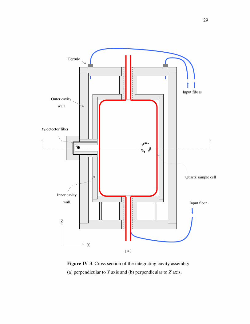
TABLE IV-1 Typical 8º hemispherial reflectance for Spectralon® SRS-99 ....................33

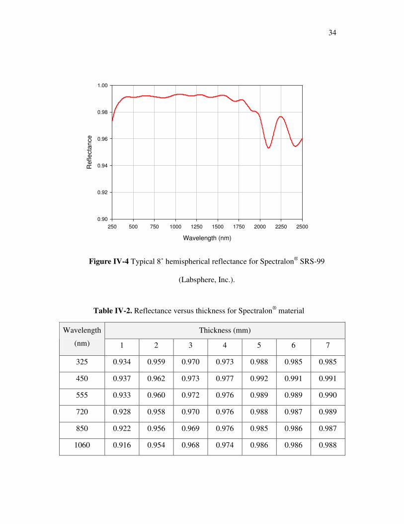
TABLE IV-2 Reflectance versus thickness for Spectralon® at 450 nm ...........................34

TABLE V-1 The absorption coefficients of pure water ..................................................77

TABLE V-2 Mode assignments with the predicated wavelengths. .................................83

1

CHAPTER I

INTRODUCTION

1.1 Optical Absorption of Water

The absorption and scattering characteristics are called inherent optical properties of

natural water (including both seawater and inland water). Absorption and scattering are

critical in determining the optical properties of the oceans; they have great applicability in

designing in situ measurements and in remote sensing of ocean waters. Knowledge of the

spectral absorption is essential to the understanding of radiative transfer in the oceanic

water column. The profiles of optical absorption in the ocean are extremely important for

tracking and understanding many of the physical processes in the ocean. In oceanography,

the study of ocean color provides insight into the abundance and concentration of

phytoplankton, sediments and dissolved organic compounds in the surface ocean waters.

The resulting information can be used to investigate biological productivity, marine optical

properties, interaction of winds and currents with ocean biology, and how human activities

influence the oceanic enviroment. The spectral absorption of pure water provides vital input

into the modeling of spectral reflectance that is important to ocean color studies.1 It also

provides a baseline for determining the diffuse attenuation coefficient and the absorption

coefficient due to dissolved or suspended organic and biological materials.2-4 The pure

water absorption spectrum plays a very important role in many other scientific disciplines,

e.g. biology, chemistry, meteorology, semiconductor processing, imaging, etc.

This dissertation follows the style of Applied Optics.

2

The spectral absorption coefficient has been studied by a large number of research groups

using a variety of techniques. There are several reviews that provide many pertinent

references to the literature.5-9 These references show notable inconsistencies due to

experimental error or sample impurity. Consequently, there has been considerable

uncertainty with regard to the correct values of the absorption coefficient of pure water in

the visible and near-visible regions.

This confusion has been largely cleared up with the data obtained by Pope and Fry10 using

their prototype Integrating Cavity Absorption Meter (ICAM).11,12 Their data provided a

major advance in accuracy, and is highly reliable due to the many crosschecks and

consistency tests.13,14 In independent studies, this data are in excellent agreement with

recent measurements of absorption coefficients for deep-sea ice,15 and with those using a

photothermal probe beam deflection technique.16,17 The importance of this new data at

wavelengths shorter than 500 nm is succinctly stated by Morel:1 “Such a drastic revision (in

the values of the absorption coefficient) is of considerable impact, in particular on the

understanding of the optical properties of extremely pure oligotrophic, waters, which form

a wide part of the world ocean. These new values, in the violet part of the spectrum,

strongly suggest that the currently admitted absorption coefficients in the near-UV (400-

300 nm) domain are likely to be also revised.”

Based on present references, there is no truly reliable data in the 300-380 nm range.

Quickenden and Irvin18 have obtained what appear to be the most often referenced data in

the 196-320 nm range, but there is no independent confirmation. Furthermore, in order to

eliminate organic contaminants that absorb in the blue and ultraviolet, Quickenden and

3

Irvin used an oxidative purification process that involved extensive contact with quartz,

sometimes at very high temperatures. In our experience high purity water samples that have

been in extensive contact with quartz or glass have significantly increased absorption in the

blue. With the ICAM we have been able to monitor this increase in absorption as a function

of the storage time in quartz containers. The concern is further highlighted by the relatively

large values for the absorption coefficient in the 390-450 nm range obtained by Litjens,

Quickenden, and Freeman19 using the similar oxidative purification process as Quickenden

and Irvin did previously.

1.2 ICAM

Natural water has a narrow transmission window in the visible region of spectrum. In a

large portion of this region (including both the blue and green spectrum) and in the UV-A

part, the values of absorption coefficient are so low (< 0.2 m-1) that it is difficult to measure

them. Specifically, scattering effects interfer with absorption measurements. To overcome

the problems of low absorption measurements in the presence of severe scattering effects,

Elterman suggested the idea of integrating cavity spectroscopy20. Fry et al.11,12 adopted this

concept to develop the ICAM; excellent absorption data for pure water were obtained by

using the ICAM. Mathematical Monte Carlo modeling shows that the operation of the

ICAM is essentially unaffected by scattering,11 in agreement with the experimental

observations of Fry et al.12. Kirk21 has also modeled the ICAM and has proposed a variant,

the Point Source ICAM, or PSICAM. The key feature of the ICAM is that it produces an

isotropic and homogeneous illumination of the liquid sample and thereby eliminates

4

scattering effects. To achieve this, the ICAM has a configuration shown in Fig. I-1. It

consists of two concentric cylinderical integrating cavities, the outer cavity and the inner

cavity, whose walls are made of a highly diffuse, reflective material with a relatively flat

spectral response over most of the UV-VIS-NIR. The liquid sample is placed inside the

inner cavity, which is surrounded by the outer cavity wall. Light is introduced into the

space between the two cavities and creates a relatively diffuse and uniform light field as a

consequence of multiple reflections due to high reflectivity of the walls. A small portion of

light passes through the inner cavity wall, leading to an isotropic illumination, from which

light is absorbed by the sample at a rate related to the absorption coefficient.

related to the absorption coefficient. Two optical fibers, located at the midpoint of each

cavity wall, are used to sample the irradiance inside the inner cavity and the irradiance in

the area between the inner and the outer cavity. By monitoring the change in irradiance

Figure I-1. Cross section of a generic ICAM

Output

Input

5

between the case when there is no sample inside the cavity (called Empty Cavity) and the

case when the cavity is filled with sample (called Full Cavity), the relative absorption

coefficient can be obtained. Similarly, by replacing the sample with calibration solutions

whose absorption coefficients are accuately known, the absolute absorption coefficient can

be determined.

There are two major advantages associated with the ICAM. First, the sample is

isotropically illuminated so the measurement is independent of scattering effects. Second,

due to the high reflectivity of cavity wall, the photons undergo many internal reflections

before they are absorbed by the sample so the total effective optical path length can be up

to sereral meters.12,22 As a consequence, even very small absorption coefficients (as low as

0.001 m-1 level) can be measured with the ICAM. An example is the absorption spectrum

of pure water measured by Pope and Fry.10

1.3 Objectives

The primary objective of this research effort is to modify the early version of the ICAM

and to extend the measurements into the UV region. The data in the 300-400 nm range will

fill a very important gap in available information. Other research goals are: to improve the

accuracy in the absorption measurements at the minimum of pure water absorption; to

investigate the apparent fact that contact of ultra-pure water with glass and quartz leads to

increased absorption in the blue to near ultraviolet range; to study, build, and to test a long

tubular form of integrating cavity with the objective of an in situ device that can directly

measure both the absorption and scattering coefficient for natural waters.

6

CHAPTER II

BACKGROUND

2.1 Theory

Consider a liquid sample placed in an isotropic homogeneous light field. The power

absorbed by the sample is independent of scattering effects and can be written as a linear

function of the absorption coefficient,10,12,22

where V is the sample volume and Fout is the outwardly directed irradiance at the surface of

the sample.

A form of more practical use is obtained by relating Eq. (2.1) to the generic model of the

ICAM as shown in Fig. II-1. According to energy conservation, the power entering the

sample volume V is equal to the power leaving the sample volume plus the power absorbed

by the sample:

Combining this with Eq. (2.1) gives

where F0 = Fout.

)1.2(,4 outabs FVP α=

)2.2(.absoutin PPP +=

)3.2(,4 0FVPP outin α+=

7

The power in is proportional to the irradiance F1 in the outer cavity and the power out is

proportional to the irradiance F0 in the inner cavity. By introducing the proportionality

constants K1 and K0, the energy conservation equation becomes

As shown in Fig. II-1, the irradiances F1 and F0 are sampled by optical fibers and converted

to voltage signals S1 and S0, respectively, by detectors D1 and D0. So Eq. (2.4) can be

rewritten as

Figure II-1. Cross section of a generic model of the ICAM

Output

Input

F1

Fo

V

Do

D1

S1

So

� S

)4.2(.4 00011 FVFKFK α+=

)5.2(4 00011 SVSCSC α+=

8

Here K1 and K0 are replaced by new proportionality constants C1 and C0. To simplify this

equation, dividing Eq. (2.5) by C1S0 gives

Replacing S1/S0 by S (so called the ICAM signal) and replacing C0/C1 by C0' leads to

Solving for the absorption coefficient � gives

This simple relation is the working equation for the ICAM.

2.2 Calibration Methods

The implementation of ICAM requires determination of C1' and C0', usually called the

calibration constants. C1' is difined as overall normalization constant and C0' is the offset

constant. Two partial derivatives derived from Eq. (2.7) and (2.8) will be particularly useful

during calibration procedures:

)6.2(.4

11

0

0

1

CV

CC

SS α+=

)7.2( '.4

01

CCV

S += α

)8.2( ).'-(')'(4 010

1 CSCCSV

C≡−=α

)9.2( ,4

1

αα CV

S =∂∂

)10.2( , '4 1

1 CV

CS

V

≡=∂∂α

9

For an ideal integrating cavity, C1' and C0' are constant numbers independent of � at fixed

wavelength. It is straightforward to determine these constants. For the special case when

there is no sample placed inside the inner cavity, � is just zero. Substituting � = 0 into Eq.

(2.8) simply gives C0' = SE. Here the signal S is denoted by the empty cavity signal SE to be

distinguished from the full cavity signal SF, which is the signal in the case when the inner

cavity is filled with a sample. Another calibration constant C1' can be determined by

measuring the signals for different calibration solutions whose absorption coefficients are

accurately known, and then by determining the slope of the plot of � versus S (i.e., ��/�S),

see Eq. (2.10).

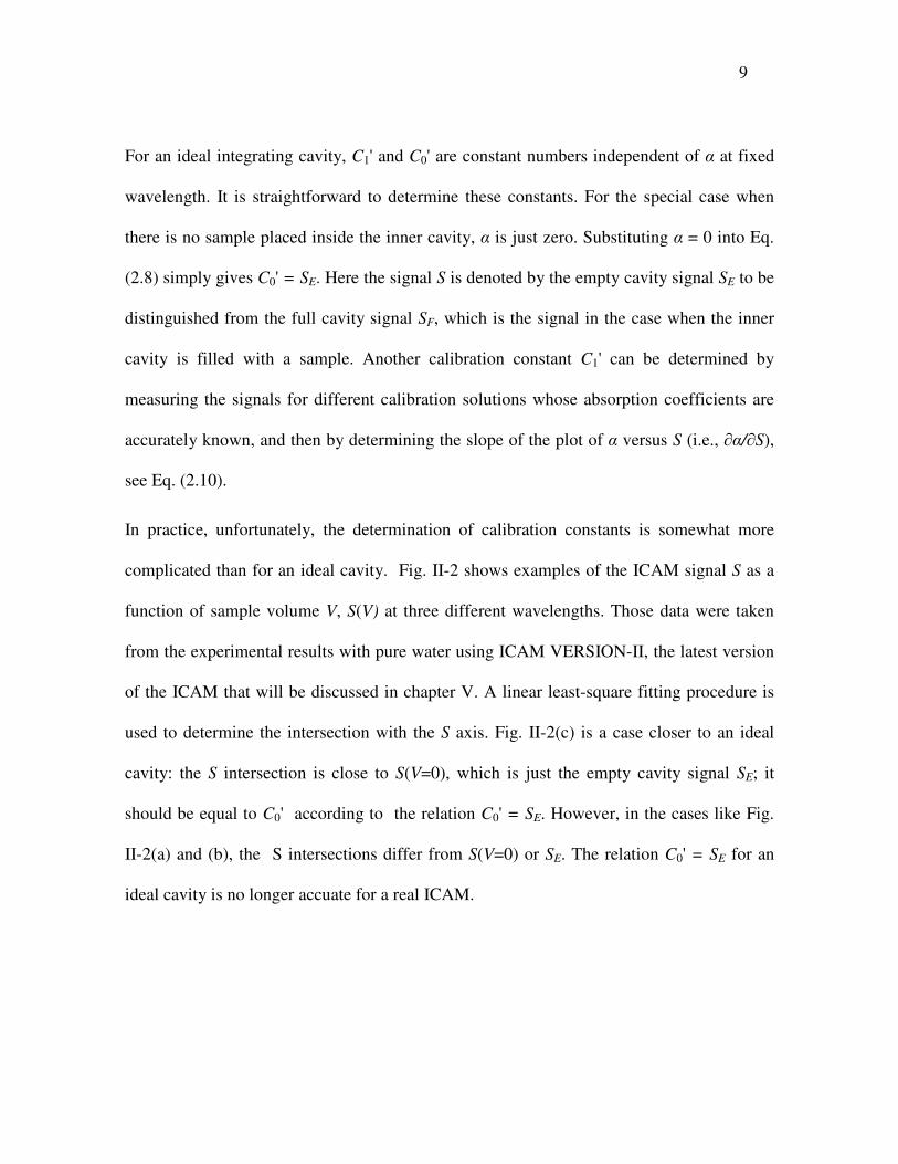
In practice, unfortunately, the determination of calibration constants is somewhat more

complicated than for an ideal cavity. Fig. II-2 shows examples of the ICAM signal S as a

function of sample volume V, S(V) at three different wavelengths. Those data were taken

from the experimental results with pure water using ICAM VERSION-II, the latest version

of the ICAM that will be discussed in chapter V. A linear least-square fitting procedure is

used to determine the intersection with the S axis. Fig. II-2(c) is a case closer to an ideal

cavity: the S intersection is close to S(V=0), which is just the empty cavity signal SE; it

should be equal to C0' according to the relation C0' = SE. However, in the cases like Fig.

II-2(a) and (b), the S intersections differ from S(V=0) or SE. The relation C0' = SE for an

ideal cavity is no longer accuate for a real ICAM.

10

Volume (ml)

0 100 200 300 400 500

S

0.126

0.128

0.130

0.132

0.134

0.136

0.138

0.140

wavelength = 400 nm

Volume (ml)

0 100 200 300 400 500

S

0.120

0.125

0.130

0.135

0.140

0.145

0.150

0.155

0.160

wavelength = 500 nm

Volume (ml)

0 100 200 300 400 500

S

0.10

0.15

0.20

0.25

0.30

0.35

0.40

wavelength = 600 nm

The complexity comes from several perturbations of the irradiance during measurement

process. First, the irradiance is perturbed by leakage of optical power due to several holes

in the cavity wall: for each cavity (outer or inner) there is a hole for the detector at

midpoint; and two more significant holes at the top and bottom to allow the sample to flow

through the cavity. Second, the index of refraction effects on outgoing irradiance F0 in the

vicinity of detector lead to systematic change from the empty cavity signal S(0) � SE, to the

half full (approximatiely) cavity signal S(280) � SH, and the full cavity signal S(566) � SF.

Figure II-2. Examples of the signal S as a function of the volume V

at three wavelengths. Also shown is the linear least-square fit.

(a)

(b) (c)

11

Specifically, optical coupling to the fiber changes as the water level rises past the fiber

monitoring F0. All these perturbations lead to an effective sample volume Veff that is

different from the actual V. Furthermore, as the consequence of their effects on irradiance,

the offset constant C0' can depend on the sample absorption � that is related to the slope

�S/�V. In order to calibrate the ICAM, this dependence must be identified and excluded. A

working equation analogous to Eq. (2.8) has been developed together with new definitions

of the two calibration constants.

2.2.1 Offset Calibration

This calibration prodedure is as following: the ICAM is filled with sequentially increasing

volume of pure water; at each volume, S is measured and recorded at fixed wavelengths

over the entire spectral range of interest; finally, at each wavelength S is plotted as a

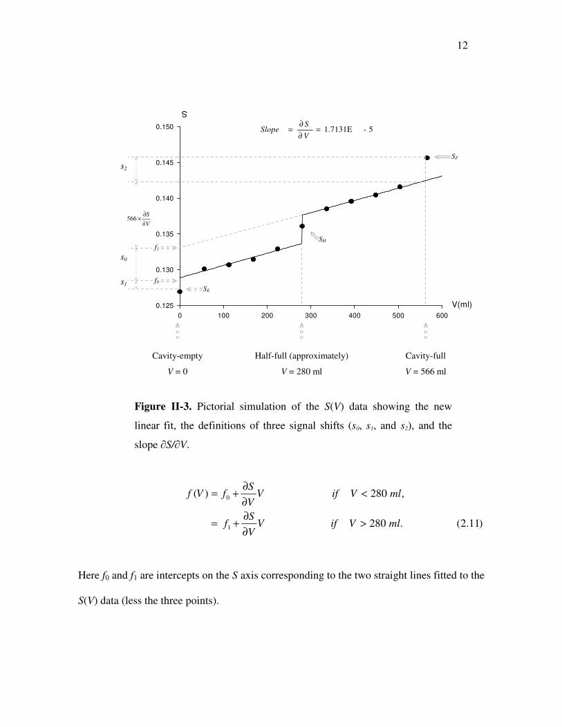
function of V. As characterized in Fig. II-3, there are three notable signal shifts. These

systematic shits are caused by the index of refraction change when the liquid sample level

approaches the midpoint of the inner cavity where the F0 detector fiber is located, and by

effects of the perturbation on the irradiance distributions at the bottom and top of the

cavity. The shifts, s0(�), s1(�), and s2(�) are designated the center shift, the cavity-empty

shift, and the cavity-full shift. It should be emphasized that the liquid sample does not

directly contact the cavity wall, rather, it is in a quartz cell in the inner cavity. The quartz

cell has a total capacity of 566 ml. Since SE, SH, and SF exhibit systematic deviations, these

three data points are excluded during the fitting process. We define a fitting function of the

form

12

V(ml)0 100 200 300 400 500 600

S

0.125

0.130

0.135

0.140

0.145

0.150

Here f0 and f1 are intercepts on the S axis corresponding to the two straight lines fitted to the

S(V) data (less the three points).

)11.2(.280

,280)(

1

0

mlVifVVS

f

mlVifVVS

fVf

>∂∂+=

<∂∂+=

s1

s0

s2

5-1.7131E=∂∂=

VS

Slope

VS

∂∂

×566

Cavity-empty

V = 0

Half-full (approximately)

V = 280 ml

Cavity-full

V = 566 ml

Figure II-3. Pictorial simulation of the S(V) data showing the new

linear fit, the definitions of three signal shifts (s0, s1, and s2), and the

slope �S/�V.

f0

f1

SE

SH

SF

13

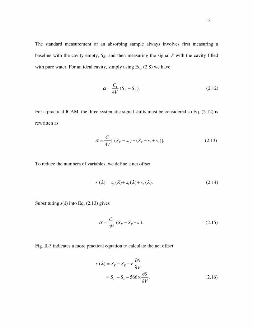
The standard measurement of an absorbing sample always involves first measuring a

baseline with the cavity empty, SE; and then measuring the signal S with the cavity filled

with pure water. For an ideal cavity, simply using Eq. (2.8) we have

For a practical ICAM, the three systematic signal shifts must be considered so Eq. (2.12) is

rewritten as

To reduce the numbers of variables, we define a net offset

Substituting s(�) into Eq. (2.13) gives

Fig. II-3 indicates a more practical equation to calculate the net offset:

)12.2().(4

1EF SS

VC −=α

)13.2()].()([4 102

1 ssSsSV

CEF ++−−=α

)14.2().()()()( 210 λλλλ ssss ++=

)15.2().(4

1 sSSV

CEF −−=α

)16.2(.566

)(

VS

SS

VS

VSSs

EF

EF

∂∂×−−=

∂∂−−=λ

14

Replacing the �S/�V by using Eq. (2.9) we have

which shows that the net offset s(�) depends on the absorption coefficient � as expected

from the discussion at the beginning of this section. This dependence must be isolated to

calibrate the ICAM. We define a general function

where we assume a simple linear dependence on wavelength � combined with a linear

dependence on slope �S/�V for s(�). Coefficients ki (i = 1,2,3,4) are determined by a least-

squares fit to the s(�) data which are directly evaluated from the experimental data S(V)

using Eq. (2.16).

Substituting Eq. (2.18) into Eq. (2.16) gives

Solving for � gives the final working equation for our experimental realization of ICAM:

)17.2(,4

566)(1

αλC

SSs EF ×−−=

)18.2(,)()( 4321 VS

kkkks∂∂+++= λλλ

)19.2(.4

)(4

)(4

14321

1

43211

��

��

�+−−−−=

��

��

�

∂∂+−−−−=

CkkkkSS

VC

VS

kkkkSSV

C

E

E

αλλ

λλα

)20.2( )."-(" 01 CSSC EF −=α

15

Where the two new calibrtion constants for normalization and offset are

C1" and C0" are completely independent of absorption coefficient �. It should be noted that

C0" is evaluated in practice via Eq. (2.22), while C1" is determined as discussed in the

following section.

2.2.2 Normalization Calibration

This calibration involves the measurement of reference samples of accurately known

absorption coefficients. Reference samples were made by dissolving dyes in pure water.

During this calibration process, the ICAM output signal SF for dye solution consists of the

signal due to the dye itself (Sdye) and the signal due to the pure water solvent (Spure water). In

order to use ICAM to measure the pure water absorption, Spure water must be isolated.

Starting with the simple relation

From Eq. (2.20), for dye solution we have

)22.2(."

)21.2(,)(4

"

210

43

11

λ

λ

kkC

kkVC

C

+=

++=

)23.2( .waterpuredyesolution SSS +=

)24.2( )."( " 01 CSSC Esolutionwaterpuredye −−=+ αα

16

Similarly, for pure water solvent we have

Eq. (2.24) minus Eq. (2.25) gives

In analogy with Eq. (2.10), the normalization constant C1" can be written as

The calibration procedure is as following: a pure water sample and a series of reference dye

solutions of accurately known absorption coefficients are prepared; the ICAM is filled with

these samples starting with pure water and then samples with sequentially higher

absorption; for each sample, S is measured and recorded at the same wavelengths as in the

offset calibration process; the pure water sample signal Spure water is subtracted from the

signal Ssolution for each dye solution to obtain Sdye (Sdye = Ssolution - Spure water, Eq.(2.23));

finally, at each wavelength, Sdye is plotted as a function of the corresponding �dye. Fig. II-4

shows examples of the signal Sdye as a function of the absorption coefficient �dye, �(S) at

three different wavelengths. These data are taken from experimental results using ICAM

)25.2( )."( " 01 CSSC Ewaterpurewaterpure −−=α

)26.2( "

).( "

1

1

dye

waterpuresolutiondye

SC

SSC

=

−=α

)27.2( . "1dye

dye

SC

∂∂

=α

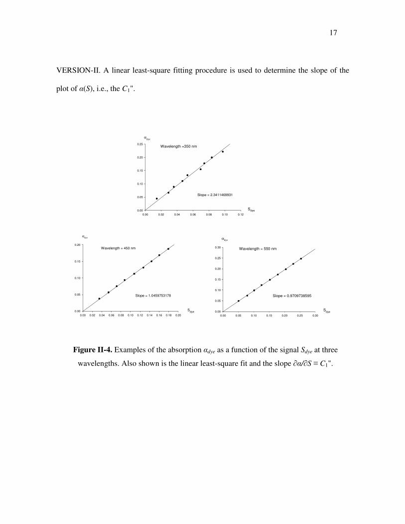
17

VERSION-II. A linear least-square fitting procedure is used to determine the slope of the

plot of �(S), i.e., the C1".

Slope = 2.3411469931

Sdye

0.00 0.02 0.04 0.06 0.08 0.10 0.12

αdye

0.00

0.05

0.10

0.15

0.20

0.25Wavelength =350 nm

Slope = 1.0459753178

Sdye0.00 0.02 0.04 0.06 0.08 0.10 0.12 0.14 0.16 0.18 0.20

αdye

0.00

0.05

0.10

0.15

0.20Wavelength = 450 nm

Slope = 0.9709738595

Sdye0.00 0.05 0.10 0.15 0.20 0.25 0.30

αdye

0.00

0.05

0.10

0.15

0.20

0.25

0.30 Wavelength = 550 nm

Figure II-4. Examples of the absorption �dye as a function of the signal Sdye at three

wavelengths. Also shown is the linear least-square fit and the slope ��/�S � C1".

18

CHAPTER III

PURE WATER

3.1 Water Purification

Water is the most widely used laboratory chemical. The definitions of pure water are

various depending on the applications. To specify the purity of the water, many standards

are published by the professional organizations such as the Ad Hoc Committee for

Laboratory Reagent-Grade Water Standards (Ad Hoc), the American Chemical Society

(ACS), the American Society for Testing and Materials (ASTM), the College of American

Pathologists (CAP), the International Organization for Standardization (ISO), the National

Committee for Clinical Laboratory Standards (NCCLS) and the United States

Phamacopeial Convention, Inc (USP). These standards are based on factors such as

electrical resistance, metal ion content, and organic or microbial contaminants present in

water. In this research study we are interested in “optical pure” water. The “absolutely

pure” water is non-existent since ultrapure water leaches contaminants from its enviroment

and is sometimes refered to “hungry” water.23

Usually, water with a resistivity of 18 megohms-cm at 25°C (the minimum limit of ASTM

Type-I water) is defined as Type-I reagent grade water. Type-II analytical grade water is

defined as having at least 1 megohm-cm resistivity. However, to only measure resistivity is

inadequate. Water at the theoretically pure limit of 18.2 megohm-cm may still contain high

concentrations of neutral organic contaminants which may adversely affect analytical

19

methods and cause analyses to fail. 24 The existence of organic matter will especially

increase the absorption in the ultraviolet region.25

Water purification methods include distillation, active carbon adsorption, microporous

membrane filtration, reverse osmosis (RO), electrodeionisation, UV treatment, and

ultrafiltration. Each method has advantages and disadvantages. For instance, water triply

distilled in quartz may still have some organics with low boiling points; the organic and

microbial contaminants in water that has been treated with ion exchange can be killed and

removed with ozone, UV, ultrafiltration, etc., but these steps can reduce the resistivity of

the water somewhat.26 Currently, most commercial systems are using a combination of

these methods to generate ultrapure ionic-free/ organic-free water.

The pure water samples used in this project are from a Millipore water purification

system,27 which consists of three subsystems: Elix 10, 60 litres polyethylene reservoir, and

Milli-Q with A10 TOC option, as shown in Fig. III-1.

Elix 10 produces Type-II quality water from potable tap water by combining several

purification technologies. Tap water initially passes through a ProgardTM pretreatment pack,

which is designed to remove particles and free chlorine from the feed water. In addition, it

helps to prevent mineral scaling in hard water areas. The water is pressurized with a pump

and then is purified by reverse osmosis (RO) to generate intermediate quality water. Next,

the RO product water passes through an electrodeionisation (E.D.I.) module to reduce

levels of organic and mineral contaminants. The typical resistivity of Elix 10 product water

is 10-15 M�-cm and the total organic carbon (TOC) is less than 30 �g / litre (ppb).

20

A 60 litre polyethylene reservoir is used for temporary storage of Elix 10 product water. On

the top there is a vent filter used to filter any air entering the reservoir. An overflow tube is

connected between the reservoir and a checkvalve. The checkvalve prevents air from

entering the reservoir through the overflow tubing. A water level sensor is installed to

display the amount of water inside the reservoir. For convenience, a valve is located on the

front of the reservoir to be used to fill beakers or other containers with water directly from

the reservoir. It is suggested that the reservoir should be drained if it is not used for over

one week.

Tap water

B A C D

E

F G H I J

K

L

A. Progard pretreatment pack

B. Booster pump C. Reverse osmosis (RO)

cartridge D. E.D.I. module E. 60 L polyethylene

reservoir F. Pump G. Q-Gard pack H. UV lamp I. Quantum ultra-pure

cartridge J. Ultra-filtration cartridge K. A10 TOC monitor L. 0.22 �m final filter

Valve

Valve

Type-II water

Type-I water

Elix 10 pure water system

Milli-Q pure water system

Figure III-1. Block diagram of the Millipore water purification system

21

The Milli-Q system is used as a final water purification stage. The feedwater comes from

Elix 10 product water temporarily stored in the 60 litre reservoir. It produces water of

Type-I quality, which is equal to or better than ASTM, CAP and NCCLS Type-I water

quality standards. Pre-treated water enters the system and is pumped through the Q-Gard

cartridge for an initial purification. Then the water is exposed to UV light at both 185 and

254 nm to oxidise organic compounds and to kill bacteria. The function of the Quantum

cartridge is to remove trace ions and oxidation by-products produced by the action of the

UV light. Purified water then passes through an Ultrafiltration (UF) module. The UF

module acts as a barrier to colloids, particles and organic molecules with a molecular

weight greater than 5000 Daltons. A manual 3-way valve directs ultrapure water through a

final 0.22 �m membrane filter so that any particles or bacteria greater than 0.22 �m will be

removed. An A10 TOC monitor is installed to measure the sample of ultrapure water to

determine trace organic levels. This special feature makes real-time organic content

monitoring a reality.

Unless otherwise noted, references to pure water in this dissertation refer to Millipore

Type-I ultrapure water with the specifications: the resistivity is consistently 18.2 M�-cm

and the total organic carbon (TOC) is from 3 to 4 �g / litre (3-4 ppb).

3.2 Sample Preparation

During preparation for an absorption measurement, all the glass or quartz containers,

tubings, valves, and the ICAM sample cell are thoroughly washed with an acid cleaning

solution,28,29 that is made by dissolving potassium dichromate in Type-II water and then

22

mixing with sulfuric acid. The acid cleaning procedure is followed by rinsing 6-8 times

with Type-II water followed by rinsing 4-6 times with Type-I water. Finally, high purity

Nitrogen gas is used for blow drying.

In the measurement process, all pure water samples are drawn from Millipore system

directly into the ICAM without any intermediate storage. This real-time feature minimizes

time and possible contamination during sample delievery.

23

CHAPTER IV

ICAM VERSION-I

4.1 System Overview

In order to extend the measurement range of the ICAM (previously developed by Dr. Pope

for his dissertation research22 and later on improved by Liqiu Cui for her master thesis23)

into the ultraviolet, several modifications have been done. The modified ICAM was named

ICAM VERSION-I.

Xenon Arc lamp

Light Shutter

Monochromator

High purity N2

Lock-in

Amplifiers

PMT

Computer with

LabView Program

& IEEE-488

Controller

Light

Chopper

Water Purification

System Quartz Tube

ICAM

Figure IV-1. Block diagram of the ICAM VERSION-I.

24

All the optics were changed to make them UV compatible, including the Xenon arc lamp,

monochromator, input fibers to the integrating cavity, and the sampling/detection fibers. A

new water purification system, Millipore Elix10 combined with Gradient A10, was

installed close to the ICAM apparatus. This new system simplifies the sample handling

procedures; it directly provides fresh purified water samples without transfers between

containers. To exclude oxygen and other contaminants, a new sample delivery system was

implemented so that pure water samples only come in contact with quartz and are always

sealed by high purity nitrogen gas (99.998%) during the measurements. Figure IV-1 shows

a block diagram of the ICAM VERSION-I.

4.2 Apparatus

4.2.1 Illumination System

The arc lamp is the light source for the ICAM. Two different Oriel lamp systems have been

used for the absorption measurement. The low power lamp system consists of an Oriel

6255 150 W ozone free xenon lamp, an Oriel 66005 lamp housing, and an Oriel 68700 200

W lamp power supply. An Oriel 6214 liquid fitter is mounted between a 3-inch f /0.7

Aspherab® UV grade fused silica condenser and a 3-inch f /3.0 fused silica secondary

focusing lens. The liquid water filter is used to remove undesired infrared radiation.30 It

uses a fused silica window to transmit down to 250 nm and is filled with Type-I pure water.

It also has an external chamber for circulation of cooling water supplied by the university

chilled water system. The high power lamp system was introduced to gain more power in

the UV, especially for measurements below 300 nm. It consists of an Oriel 6269 1000 W

25

xenon lamp, an Oriel 66923 lamp housing, and an Oriel 68920 1000 W lamp power supply.

To reduce hazardous ozone, an Oriel 66087 ozone eater is required whenever the lamp is

ignited. As with the low power system, an Oriel 6227 liquid water filter is used to remove

infrared radiation. Unfortunately, the liquid fitlter alone was not sufficient to ensure the

monochromator and the optical shutter against damage caused by exposure to the high

power radiation. For experiments over a short period of time, a 3-inch CVI UR-3 UV

reflecting mirror operating at 45º incident angle was used. The mirror transmits most of the

red and IR to an air-cooled heatsink and reflects the shorter wavelength radiation into the

monochromator.31 For experiments over longer period of time, we specifically designed a

prism with a 30º apex angle that provides sufficient wavelength dispersing to avoid optical

damage at the focal points. The prism is mounted on a translation stage. We adjust the

position of the stage to ensure the desired spectral region is forcused on the entrance slit of

the monochromator. The rest of the light is blocked by an aperture. Fig. IV-2 shows a top

view of experimental set-up for the prism. The body of prism is stainless steel. The two

windows are 3-inch Esco S1-UV grade fused silica square plates. The cell is filled with

Type-I pure water which served as both the prism medium for dispersing the light and as an

absorber for removing the IR. A hole was drilled through the entire prism body and was

connected to the university chilled water system. Cooling water first passes through the

prism and then through a Lytron 6110G1SB liquid-to-air heat exchanger that is mounted on

the lamp housing to cool the air flowing to the ozone eater.

26

The light Shield is made of black corrugated PVC pipe. It shields the beam between the arc

lamp and the optical shutter from dust and stray light.

The shutter is used to control the light entering the monochromator. A Copal DC-494

plunger shutter with a 30 mm diameter, 5 blade assembly is attached to the alluminum

cover plate in front of the entrance slit of the monochromator. Closing this shutter allows

measurement of the ICAM background signal due to PMT dark current and stray light. The

shutter is powered by a DC 24 V plug-top transformer, which is controlled by an HP 6214A

power supply. The shutter defaults to close when power is off.

The monochromator is a CVI Digikrom 240 classical Czerny-Turner monochromator with

a 240 mm focal length and an effective aperture ratio of f / 3.9.32 It can be controlled either

by a control module through an RS-232C serial port, or by a computer through a GPIB

(IEEE 488) interface. Typically, the former control mode is used for testing or quick

Prism

Focus lens

Entrance slit of monochromator

Light from arc

lamp

Water

Figure IV-2. Top view of experimental set-up for the dispersing prism.

27

adjustment and the latter is the primary instrument control during absorption measurements.

Digikrom 240 has a reversible, two-grating mount with two 1200 grove/mm gratings. The

gratings are designated as #1 and #2 on the LCD of the control module. The peak

transmissions of grating #1 and #2 are at 500 nm and 330 nm respectively. When

continuously scanning from UV to IR, the grating must be changed from #2 to #1 at 620

nm. The reciprocal linear dispersion of the Digikrom 240 is 3.2 nm/mm and the spectral

resolution is 0.06 nm with a 20 micron slit width. The optics inside the monochromator was

coated with UV protected aluminum (PAUV).33

Input Fiber Assembly consists of six 1.5 m long silica-core, silica-clad optical fibers with

600 �m core diameter and 1.0 mm cladding diameter. Each fiber is shielded in furcation

tubing (protective cable). This custom-made assembly from C Technologies, Inc.22 is used

to couple the light from the monochromator into the integrating cavity. At the input end the

six fibers are arranged in a linear array and embedded in an aluminum ferrule, which is

secured in a transparent Plexiglas block by a set screw. The orientation of the linear fiber

array with respect to the exit slit, and the distance between the fiber and the exit slit can be

adjusted and locked with the set screw. The Plexiglas block is mounted on a Newport X-Y

translation stage attached to the cover plate in front of the exit slit of the monochromator; it

is used to adjust the transverse position of the fiber relative to the exit slit. At the output end

each fiber terminates in an aluminum ferrule for protection. The output end of each fiber

extends about 1.3 cm beyond from the ferrule and through a 1 mm I.D. hypodermic tube.

All the fiber ends are polished by Thorlabs polishing films (5 �m film followed by 3 �m

and 1 �m films).

28

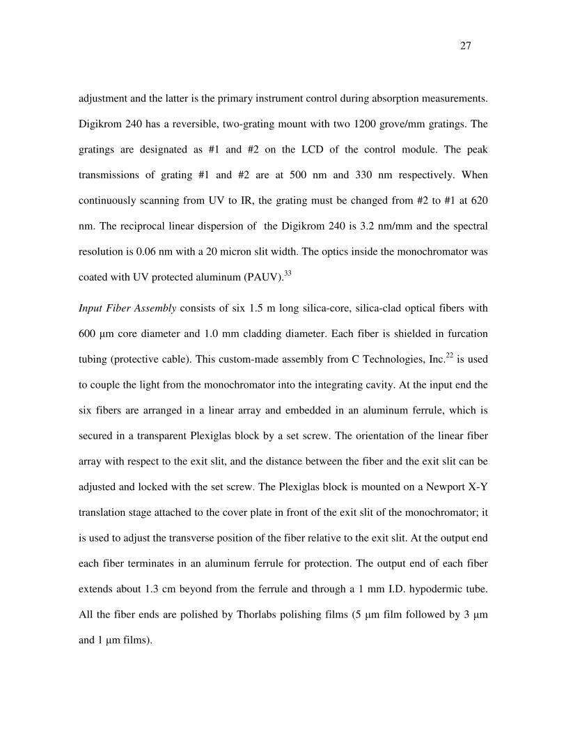
4.2.2 Integrating Cavity Assembly

The integrating cavity assembly is the critical part of the ICAM. It consits of two concentric

integrating cavities and a Heraeus Suprasil quartz sample cell with inlet and outlet quartz

tubes. The entire assembly is in a black light-tight Plexiglas box to shield it from external

light sources. The box has ports for both inlet and outlet tubes, for the six input fibers (three

at the top and three at bottom respectively), and for the two detector fibers described later

in this section. All ports are sealed with black electrical tape. Fig. IV-3 shows cross sections

of the integrating cavity assembly.

In Fig. IV-3 (b), viewed along the Z axis, the outer cavity has a hexagonal cross section

with 107 mm between the inside faces. Its wall is made of six interlocking Spectralon®

plates 12.7 mm thick and 254 mm high. Two 19 mm holes are drilled in the wall to mount

the detectors. The outer cavity is closed by two 12.7 mm thick Spectralon® end caps. Each

hexagonal cap has a 19 mm center hole for the sample cell inlet or outlet tube, and three 2

mm holes for the input fibers. The caps have three holes, 120º apart on a 113 mm diameter

circle; on one cap they are offset by 60º with respect to those in the other cap.

29

Input fibers

Input fiber

Ferrule

X

Z

Figure IV-3. Cross section of the integrating cavity assembly

(a) perpendicular to Y axis and (b) perpendicular to Z axis.

( a )

Inner cavity

wall

Quartz sample cell

Outer cavity

wall

F0 detector fiber

30

The inner cavity is a 151 mm high Spectralon® cylinder with a 101.6 mm O.D., an 89 mm

I.D., and two round Spectralon® end caps. Each end cap is 12.7 mm thick with a 19 mm

hole in the center. The inner cavity is held at the midpoint of the outer cavity by

Spectralon® tubes at the center and three additional Spectralon® dowels symmetrically

F1 detector fiber

F0 detector fiber

Aluminum foil

Dowel

Input fiber X

Y

(b)

Figure IV-3. Continued.

31

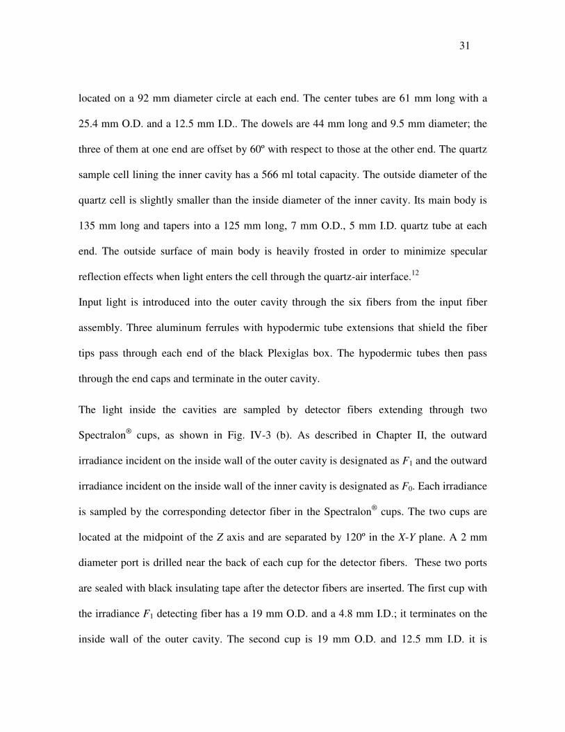
located on a 92 mm diameter circle at each end. The center tubes are 61 mm long with a

25.4 mm O.D. and a 12.5 mm I.D.. The dowels are 44 mm long and 9.5 mm diameter; the

three of them at one end are offset by 60º with respect to those at the other end. The quartz

sample cell lining the inner cavity has a 566 ml total capacity. The outside diameter of the

quartz cell is slightly smaller than the inside diameter of the inner cavity. Its main body is

135 mm long and tapers into a 125 mm long, 7 mm O.D., 5 mm I.D. quartz tube at each

end. The outside surface of main body is heavily frosted in order to minimize specular

reflection effects when light enters the cell through the quartz-air interface.12

Input light is introduced into the outer cavity through the six fibers from the input fiber

assembly. Three aluminum ferrules with hypodermic tube extensions that shield the fiber

tips pass through each end of the black Plexiglas box. The hypodermic tubes then pass

through the end caps and terminate in the outer cavity.

The light inside the cavities are sampled by detector fibers extending through two

Spectralon® cups, as shown in Fig. IV-3 (b). As described in Chapter II, the outward

irradiance incident on the inside wall of the outer cavity is designated as F1 and the outward

irradiance incident on the inside wall of the inner cavity is designated as F0. Each irradiance

is sampled by the corresponding detector fiber in the Spectralon® cups. The two cups are

located at the midpoint of the Z axis and are separated by 120º in the X-Y plane. A 2 mm

diameter port is drilled near the back of each cup for the detector fibers. These two ports

are sealed with black insulating tape after the detector fibers are inserted. The first cup with

the irradiance F1 detecting fiber has a 19 mm O.D. and a 4.8 mm I.D.; it terminates on the

inside wall of the outer cavity. The second cup is 19 mm O.D. and 12.5 mm I.D. it is

32

inserted through the outer cavity wall and terminates in the wall of the inner cavity as

shown in Fig. IV-III. Another Spectralon® cup with 12.5 mm O.D. and 6 mm I.D. is

pressed into the second cup with an aluminum foil embeded between them to prevent cross

talk between the two irradiances F1 and F0. The irradiance F0 detecting fiber extends into

this cup.

Spectralon® is the material used to build both the outer and inner cavities of the ICAM.

This diffuse reflectance material exhibits relatively flat spectral distribution and gives the

highest diffuse reflectance of any previously known material or coating over the UV-VIS-

NIR region of the spectrum.34 In each case, reflection and transmission, Spectralon® is

almost perfectly lambertian. The reflectance is generally >99% over a range from 400 to

1500 nm and >95% from 250 to 2500 nm. Values of its reflectivity35 are shown in Table

IV-1 and are plotted in Fig. IV-4. The reflectance of Spectralon® also depends on it

thickness as shown in Table IV-236 and are plotted in Fig. IV-5. Spectralon®’s highly

diffuse and highly reflective performance is the key to realize the isotropic illumination of

the water sample inside the inner cavity.

33

Wavelength (nm) Reflectance Wavelength

(nm) Reflectance

250 0.973 1400 0.991

300 0.984 1500 0.992

400 0.991 1600 0.992

500 0.991 1700 0.988

600 0.992 1800 0.989

700 0.992 1900 0.981

800 0.991 2000 0.976

900 0.991 2100 0.953

1000 0.993 2200 0.973

1100 0.993 2300 0.972

1200 0.992 2400 0.955

1300 0.993 2500 0.960

Table IV-1. Typical 8˚ hemispherical reflectance for Spectralon® SRS-99

34

Wavelength (nm)

250 500 750 1000 1250 1500 1750 2000 2250 2500

Ref

lect

ance

0.90

0.92

0.94

0.96

0.98

1.00

Thickness (mm) Wavelength

(nm) 1 2 3 4 5 6 7

325 0.934 0.959 0.970 0.973 0.988 0.985 0.985

450 0.937 0.962 0.973 0.977 0.992 0.991 0.991

555 0.933 0.960 0.972 0.976 0.989 0.989 0.990

720 0.928 0.958 0.970 0.976 0.988 0.987 0.989

850 0.922 0.956 0.969 0.976 0.985 0.986 0.987

1060 0.916 0.954 0.968 0.974 0.986 0.986 0.988

Table IV-2. Reflectance versus thickness for Spectralon® material

Figure IV-4 Typical 8˚ hemispherical reflectance for Spectralon® SRS-99

(Labsphere, Inc.).

35

Thickness (mm)

0 1 2 3 4 5 6 7 8

Ref

lect

ance

0.90

0.92

0.94

0.96

0.98

1.00

reflectance

The crucial assumptions made for ICAM in chapter II is that the sample is in an isotropic

and homogeneous light field. In practice these conditions can not be exactly satisfied due to

the energy loss by the absorption of the sample or by the leakage of radiation in the area

close to the entrance or exit ports of the cavity. However, it has been shown both

experimently12,22 and by theoretical simulation21 that the isotropy and homogeneity are

sufficient in the ICAM.

Figure IV-5. Reflectance versus thickness for Spectralon® at 450 nm.

36

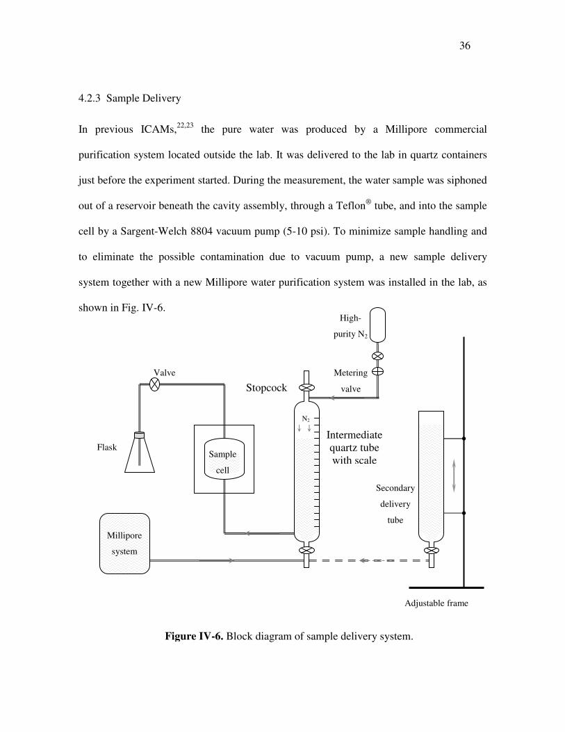
4.2.3 Sample Delivery

In previous ICAMs,22,23 the pure water was produced by a Millipore commercial

purification system located outside the lab. It was delivered to the lab in quartz containers

just before the experiment started. During the measurement, the water sample was siphoned

out of a reservoir beneath the cavity assembly, through a Teflon® tube, and into the sample

cell by a Sargent-Welch 8804 vacuum pump (5-10 psi). To minimize sample handling and

to eliminate the possible contamination due to vacuum pump, a new sample delivery

system together with a new Millipore water purification system was installed in the lab, as

shown in Fig. IV-6.

Millipore

system

Sample

cell

Flask

Stopcock Valve

Intermediate quartz tube with scale

Secondary

delivery

tube

Adjustable frame

Metering

valve

High-

purity N2

tank

N2

Figure IV-6. Block diagram of sample delivery system.

37

From the Millipore purification system, the fresh water sample flows through Teflon tube

into an intermediate quartz tube. This Chemical Glass HSQ—300 quartz tube is 1000 mm

long, 40 mm O.D., and 36 mm I.D.; it tapers into quartz capillary tubing at each end and

into a quartz stopcock. Each stopcock consists of glass barrel, PTFE plug and FETFE O-

ring. Along the quartz tube, a soft ruler with the minimum scale division of 1 mm is

attached. It is used to measure the water level inside the tube; the latter can be converted

into the volume of the water in the sample cell. With the help of high purity nitrogen gas,

the water in the imtermediate tube is pushed into the sample cell, through a 7mm O.D., 5

mm I.D. HSQ—300 quartz tube. The flow rate of nitrogen gas is controlled by the

combination of a Swagelok® metering valve and a ball valve. During measurement, the

entire sample delivery system is shield from external light by aluminum foil and black

curtain. The sample being measured is always sealed by high purity nitrogen gas to

minimize oxygen contamination.18,25 There is a secondary glass delivery tube mounted on a

frame whose height can be adjusted. Lifting the frame allows calibration dye solutions or

an acid cleaning solution in this tube to flow into the intermediate quartz tube. The

secondary delivery glass tube is 1000 mm long, 40 mm O.D., 36 mm I.D., and has a glass

stopcock at the bottom.

38

4.2.4 Detector System

As shown in Fig. IV-7, the irradiances F1 and F0 are sampled through optical fibers,

chopped by a two-channel light chopper with frequency f and f/10, respectively, and

detected by a PMT. The PMT converts the combination of chopped F1 and F0 light into a

voltage signal Smix = S1+S0 (S1, S0 are defined in Chapter II.). This approximately square

wave signal Smix provides the input to the two lock-in amplifiers. The two lock-in amplifiers

extract the amplitudes of the two components S1 and S0 which are modulated at frequencies

f and f/10, respectively. Finally S1 and S0 are sent to the computer to calculate the ICAM

signal S � S1/ S0.

The output fiber assembly consists of an aluminum fiber adaptor coated by black paint, and

two 590 mm long, 0.37 NA TECSTM coated silica/silica multimode fibers with 1.5 mm core

Input fiber

F1

F0

ICAM cavity

S1

S0

Computer

(S = S1/S0)

Oscilloscope

PMT F1 signal (f)

F0 signal (f /10)

Sync

outputs

f

f /10

Lock-in amplifiers

Fiber adaptor

Shutter Chopping

disc

Chopper

Figure IV-7. Block diagram of ICAM detector system and signal flow.

Window-I

39

diameter and 2.0 mm cladding diameter. Each fiber is shielded in furcation tubing

(protective cable) and both ends are carefully polished. The fiber adaptor positions the

output ends of the two fibers close to the corresponding channels (windows) inside the

chopper.

The light Chopper is a customized compact EG&G 197 Precision Light chopper.37 It

contains all the control circuit needed to keep the chopping disc synchronized to its internal

precision oscillator or to an external trigger. The chopper has two windows equipped with

manual shutters. Closing the shutter will block the light through the corresponding window.

The shutters are particularly useful to check for crosstalk between the two channels. The

chopping disc is made by sticking a 12 �m blade to the back disc. The blade has 30 outer

apertures and 3 inner apertures. Each set of apertures chops the light from the

corresponding window. The light through the window-I is proportional to irradiance F1,

similarly the light through the window-II is proportional to irradiance F0. The outer

apertures cover the frequency range 150-3000 Hz and the inner apertures cover the

frequency range 15-300 Hz. Once the chopping frequency is set to a value f using a four

digit pushbutton selector switch in the chopper, the light through the window-I will be

chopped at frequency f, and the light through window-II is at frequency f/10. For each

chopped signal, the amplitude is proportional to the corresponding irradiance. The chopper

has two synchronous outputs which generate a 10 V nominal peak to peak square wave at

the outer 30 aperture blade chopping frequency f, and at the inner 3 aperture blade chopping

frequency f/10. They are used as reference frequencies by the lock-in amplifiers to extract

the S1 and S0 signals from Smix. The chopper is powered by an HP 6235A triple output

40

power supply. This extremely compact chopper together with a single photomultiplier tube

reduces signal fluctuations due to random disturbances, and therefore increases the signal-

to-noise ratio.

The PMT is Burle 4840 photomultiplier tube surrounded by a magnetic shield wrapped in

electrical tape. The entire PTM housing is attached to the back of the light chopper by an

aluminum mount. A customized power supply provides –1100V to the PMT and the output

current signal is converted to a voltage signal Smix by a grounded 4.6 M� resistor.

The lock-in amplifiers are used to extract the outer cavity signal S1 at reference frequency f

and the inner cavity signal S0 at reference frequency f/10 from the PMT output signal Smix,

and send them to the computer for data analysis. The amplifier detecting S1 is a Stanford

Research System SR 830 DSP,38 and the amplifier detecting S0 is an EG&G 5210.39 Both

amplifiers are controlled by the computer via the GPIB (IEEE 488) interface.

The oscilloscope is a Tektronix 210 digital real-time oscilloscope. It is used to check the

PMT output voltage signal Smix.

4.2.5 Data Acquisition

A Macintosh Quadra 840AV equipped with a National Instruments IEEE-488 controller

provides the platform from which the ICAM is operated and controlled. The controller is

connected with the GPIB (IEEE 488) interfaces of the monochromator and the lock-in

amplifiers. The core of this computer platform consists of a group of LabVIEW programs

which are used for instrument control, data acquisition, data display, and data analysis. Fig

IV-8. shows the front panel of the main program (called VI, initials of the virture

41

instrument), ICAM-MAIN.vi. The other programs are sub-routines (sub-Vis) of the main

program.

In the front panel, we can set the following control parameters: the data file name and path,

the starting and ending positions with the interval (step) of the wavelength scan, the width

of the monochromator slits, and the number of data points to average at each wavelength.

As the ICAM-MAIN.vi starts running, it commands the monochromator to adjust the slit

width and the intial wavelength; it controls the two lock-in amplifiers and reads the values

of the voltage signals S1 and S0 extracted from Smix. Once the wavelength and signal values

Figure IV-8. Front panel of ICAM-MAIN.vi in measurement process.

42

has been collected and processed (including averaging and calculating S � S1/ S0), the

computer writes the data to a file in text format. The program then moves to the next

wavelength and the process is repeated until the final wavelength is reached. During the

measurement, the front panel shows a graph of the real-time data for the ICAM signal S

versus wavelength. If the experiment is run repeatedly, all the data are accummulated and

plotted on the front panel.

4.3 Preliminary Tests

4.3.1 UV Measurement

The previously developed ICAM has been modified to extend the measurement capability

into the UV. To check the performance after modification, a Newport 840C power meter

with an 818-UV detector was used to measure the power from the exit slit of the Digikrom

240 monochromator and from the output end of one of the six input fibers. The 150 W

Xenon arc lamp system was used with a 600 �m wide monochromator slit. Figure IV-9.

shows the measured power from the exit slit of the monochromator when different

monochromator gratings were used. Clearly, for absorption measurements in the UV,

grating #2 must be used. Figure IV-10. shows the power from the output end of a single

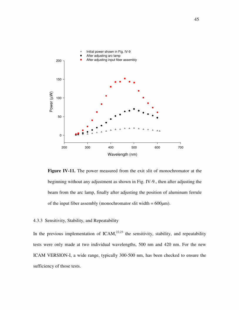
input fiber when using grating #2. Figure IV-11 shows the improvements 1) after

optimizing the beam entering the monochromator (including adjusting the image of the arc

on the entrance slit and the distance between the arc lamp and the slit) and then, 2) after

optimizing the beam coming out of the exit slit (adjusting the position of the aluminum

ferrule, which shields the input fibers, in relation to the exit slit).

43

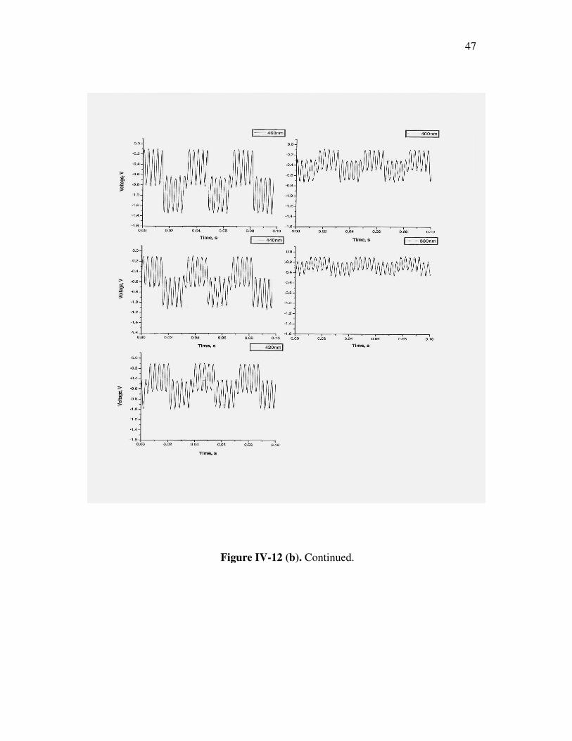
4.3.2 Signal Test

The Tektronix 210 digital oscilloscope was used to examine the PMT output signal Smix and

to check the chopping and detecting process. In Fig. IV-12 (a), (b), and (c), a few examples

taken from the oscilloscope show the chopped signal at several wavelengths and with two

different slit widths.

Wavelength (nm)

200 300 400 500 600 700

Pow

er (

µ W)

0

5

10

15

20

25

Using grating #1Using grating #2

Figure IV-9. The power measured from exit slit of monochromator with

grating #1 and #2, respectively (monochromator slit width = 600�m).

44

Wavelength (nm)

200 300 400 500 600 700

Pow

er (µ

W)

0.0

0.2

0.4

0.6

0.8

1.0

1.2

Figure IV-10. The power measured from the output end of a single input

fiber with grating #2 (monochromator slit width = 600�m).

45

Wavelength (nm)

200 300 400 500 600 700

Pow

er (µ

W)

0

50

100

150

200

Initial power shown in Fig. IV-9After adjusting arc lampAfter adjusting input fiber assembly

4.3.3 Sensitivity, Stability, and Repeatability

In the previous implementation of ICAM,22,23 the sensitivity, stability, and repeatability

tests were only made at two individual wavelengths, 500 nm and 420 nm. For the new

ICAM VERSION-I, a wide range, typically 300-500 nm, has been checked to ensure the

sufficiency of those tests.

Figure IV-11. The power measured from the exit slit of monochromator at the

beginning without any adjustment as shown in Fig. IV-9., then after adjusting the

beam from the arc lamp, finally after adjusting the position of aluminum ferrule

of the input fiber assembly (monochromator slit width = 600�m).

46

Figure IV-12 (a). The PMT output signal Smix displayed on oscilloscope

at several wavelengths. (monochromator slit width = 300�m).

47

Figure IV-12 (b). Continued.

48

Figure IV-12 (c). Continued.

49

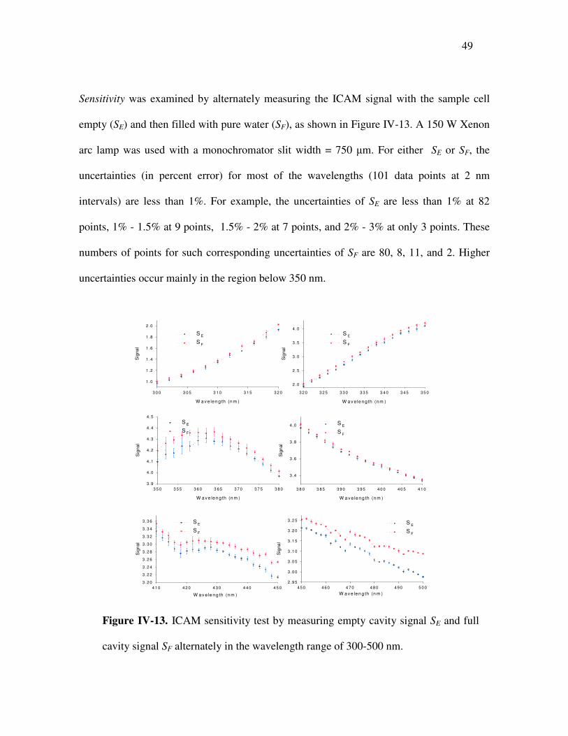
Sensitivity was examined by alternately measuring the ICAM signal with the sample cell

empty (SE) and then filled with pure water (SF), as shown in Figure IV-13. A 150 W Xenon

arc lamp was used with a monochromator slit width = 750 �m. For either SE or SF, the

uncertainties (in percent error) for most of the wavelengths (101 data points at 2 nm

intervals) are less than 1%. For example, the uncertainties of SE are less than 1% at 82

points, 1% - 1.5% at 9 points, 1.5% - 2% at 7 points, and 2% - 3% at only 3 points. These

numbers of points for such corresponding uncertainties of SF are 80, 8, 11, and 2. Higher

uncertainties occur mainly in the region below 350 nm.

W a ve len g th (n m )

3 0 0 3 0 5 3 1 0 3 1 5 3 2 0

Sig

nal

1 .0

1 .2

1 .4

1 .6

1 .8

2 .0

S E

S F

W a v e le n g th (n m )

3 2 0 3 2 5 3 3 0 3 3 5 3 4 0 3 4 5 3 5 0

Sig

nal

2 .0

2 .5

3 .0

3 .5

4 .0S E

S F


3 5 0 3 5 5 3 6 0 3 6 5 3 7 0 3 7 5 3 8 0

Sig

nal

3 .9

4 .0

4 .1

4 .2

4 .3

4 .4

4 .5S E

S F


3 8 0 3 8 5 3 9 0 3 9 5 4 0 0 4 0 5 4 1 0

Sig

nal

3 .4

3 .6

3 .8

4 .0 S E

S F

W av e le n g th (n m )

4 1 0 4 2 0 4 3 0 4 4 0 4 5 0

Sig

nal

3 .2 0

3 .2 2

3 .2 4

3 .2 6

3 .2 8

3 .3 0

3 .3 2

3 .3 4

3 .3 6 S E

S F

W a ve len g th (n m )4 5 0 4 6 0 4 7 0 4 8 0 4 9 0 5 0 0

Sig

nal

2 .9 5

3 .0 0

3 .0 5

3 .1 0

3 .1 5

3 .2 0

3 .2 5 S E

S F

Figure IV-13. ICAM sensitivity test by measuring empty cavity signal SE and full

cavity signal SF alternately in the wavelength range of 300-500 nm.

50

Stability was checked by recording the cavity-empty signal SE at given time intervals,

typically every one hour, over a period of at least 6-8 hours, as shown in Fig. IV-14.

Time t (hour)

0 1 2 3 4 5 6 7 8 9 10 11 12 13 14 15

Cav

ity-e

mpt

y si

gnal

SE

1

2

3

4

300 nm 324 nm 350 nm 374 nm400 nm 424 nm450 nm474 nm 500 nm

Repeatability was determined by recording a single measurement of cavity-empty signal SE

and cavity-full signal SF on three successive days, then calculating the signal (SE, SF)

Figure IV-14. ICAM stability test by recoding the cavity-empty signal SE at 1 hour

intervals over 14 hours, here t = 0 is the time right after turning on all the

equipment.

51

difference between successive days. The results are shown in Fig. IV-15. For both SE and

SF, the differences were on the order of ~ 1% compared to the average of SE (or SF) on

successive days.

These experimental results show the sensitivity of the ICAM VERSION-I to the changing

absorption between the empty cell and the cell filled with pure water, the stability of the

cavity-empty signal over several hours of operation, and the repeatabilities of both the

cavity-empty signal and cavity-full signal on successive days.

4.4 Absorption Measurement

Pure water absorption measurements begin by measuring cavity-empty signals SE, which

act as baseline for the ICAM, followed by measuring cavity-full signals SF at 2 nm intervals

over the entire wavelength region. Before the experiment starts, the sample cell and the

entire sample delivery system are purged with high purity nitrogen gas. Typically, both SE

and SF are repeatedly measured 5-7 times; this permits analysis of the repetitive signals to

determine the stability and repeatability of the signal, and to improve signal to noise ratio

by averaging the results. The pure water sample is changed every time SF is measured to

ensure that a fresh sample is being examined, and the samples are always sealed by high

purity nitrogen gas (99.998%).

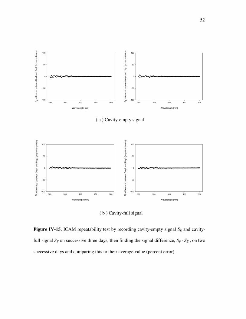
52

Wavelength (nm)

300 350 400 450 500SE

diff

eren

ce b

etw

een

Day

1 an

d D

ay2

(in p

erce

nt e

rror

)

-100

-50

0

50

100

Wavelength (nm)

300 350 400 450 500SE

diff

eren

ce b

etw

een

Day

2 an

d D

ay3

(in p

erce

nt e

rror

)

-100

-50

0

50

100

Wavelength (nm)

300 350 400 450 500SF

diffe

renc

e be

twee

n D

ay1

and

Day

2 (in

per

cent

err

or)

-100

-50

0

50

100

Wavelength (nm)

300 350 400 450 500SF

diffe

renc

e be

twee

n D

ay2

and

Day

3 (in

per

cent

err

or)

-100

-50

0

50

100

( a ) Cavity-empty signal

( b ) Cavity-full signal

Figure IV-15. ICAM repeatability test by recording cavity-empty signal SE and cavity-

full signal SF on successive three days, then finding the signal difference, SF - SE , on two

successive days and comparing this to their average value (percent error).

53

Wavelength (nm)

300 350 400 450 500 550 600

Cav

ity-e

mpt

y si

gnal

SE

1

2

3

4

Wavelength (nm)

300 350 400 450 500 550 600

Cav

ity-fu

ll si

gnal

SF

1

2

3

4

Figure IV-16. Single measurement of ICAM cavity-empty signal (left) and

cavity-full signal (right) with error bars.

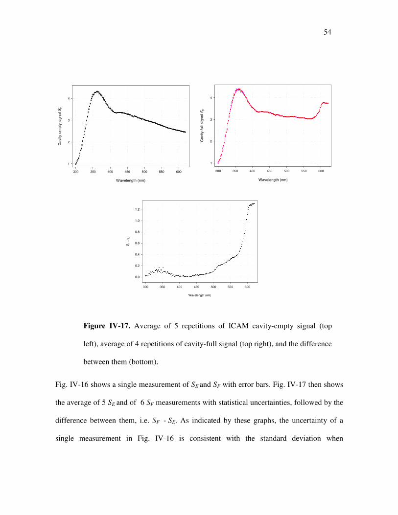
54

Wavelength (nm)

300 350 400 450 500 550 600

Cav

ity-e

mpt

y si

gnal

SE

1

2

3

4

Wavelength (nm)

300 350 400 450 500 550 600

Cav

ity-fu

ll si

gnal

SF

1

2

3

4

Wavelength (nm)

300 350 400 450 500 550 600

SF

- SE

0.0

0.2

0.4

0.6

0.8

1.0

1.2

Fig. IV-16 shows a single measurement of SE and SF with error bars. Fig. IV-17 then shows

the average of 5 SE and of 6 SF measurements with statistical uncertainties, followed by the

difference between them, i.e. SF - SE. As indicated by these graphs, the uncertainty of a

single measurement in Fig. IV-16 is consistent with the standard deviation when

Figure IV-17. Average of 5 repetitions of ICAM cavity-empty signal (top

left), average of 4 repetitions of cavity-full signal (top right), and the difference

between them (bottom).

55

repetitive measurements are averaged together in Fig. IV-17. During the absorption

measurements and both calibration procedures described in the following sections, the

temperature of the pure water from the purification system was stable at 25 °C (±1 °C),

with 18.2 M� resistivity and TOC 4 ppb (±2 ppb).

4.5 Calibration

The offset calibration is always performed before the normalization calibration because the

former only involves pure water sample but the latter involves dye solutions which can

introduce contamination to the sample delivery system.


As described in Chapter II, the offset calibration is based on the function S(V) which is the

ICAM signal S versus sample volume V obtained by measuing a set of pure water samples

with different volumes. The Calibration starts with a cavity-empty signal measurement

(defined as S(0) identical to SE), followed by measuring 10-15 pure water samples in a

sequence of equally increasing volume, until the last sample, S(566) which is identical to

cavity-full signal SF (566 is the total capacity of the sample volume in millilitre). Examples

of S(V) at several wavelengths are plotted in Fig. IV-18. During the entire measurement

process, each sample is sealed by high purity nitrogen gas.

56

Volume (ml)

0 100 200 300 400 500 600

S

0.90

0.92

0.94

0.96

0.98

1.00

1.02

1.04

W avelength = 300 nmSlope = 1 .2507e-4

Volum e (m l)

0 100 200 300 400 500 600

S

2.26

2.28

2.30

2.32

2.34

2.36

W avelength = 324 nmSlope = 1.1207e-4

Volum e (m l)

� ��

S

4.10

4.15

4.20

4.25

4.30


Volume (m l)

0 100 200 300 400 500 600

S

4.12

4.14

4.16

4.18

4.20

4.22


Volum e (m l)

0 100 200 300 400 500 600

S

3.25

3.26

3.27

3.28

3.29

3.30

3.31


Volume (ml)

0 100 200 300 400 500 600

S

3.17

3.18

3.19

3.20

3.21

3.22

3.23

3.24

3.25


Volum e (m l)

0 100 200 300 400 500 600

S

3.08

3.10

3.12

3.14

3.16

3.18


Volum e (m l)

0 100 200 300 400 500 600

S

2.96

2.98

3.00

3.02

3.04

3.06

3.08

3.10

W avelength = 500 nmSlope = 1 .7303e-4

Figure IV-18. The signal S as a function of the volume V at eight wavelengths.

Also shown is the linear least-square fitting line discussed in Chapter II.

57


As described in Chapter II, the normalization calibration is based on the function �(S)

which is the absorption coefficient � of the dye versus the ICAM signal S. It is measured by

first measuring a pure water sample, followed by measuing 8-10 dye solutions in a

sequence of increasing concentrations.

A “master” dye solution was prepared by dissolving the dye powder ( on the order of a

milligram) in pure water, then filtering the dye solution through Gelman Supor®-200 47

mm diameter, 0.2 �m membrane filters. The absorption (A) of the “master” dye solution

was measured at 1 nm intervals over the wavelength region from 200 nm to 700 nm in a

Varian Cary100 spectrophotometer in the Chemistry department. The absorption due to the

dye, Adye was obtained by placing two identical Fisher standard cells (3 ml, 10 mm

lightpath, with Suprasil quartz windows) filled with “master” dye solution and pure water,

respectively, into two equally separated beams of the spectrophotometer, then measuring

the absorption due to the dye solution Asolution, and the absorption due to pure water, Apure

water. Finally the dye absorption Adye � Asolution - Apure water is calculated and saved as a

function of wavelength. This absorption Adye is converted to absorption coefficient �dye (as

defined in Chapter II) in units of m-1 by using the following equation:

)1.4(,10ln

AL

×=α

which is simply derived from the definition of absorption used in the Chemistry lab,

)2.4(),/(log10 IIA o≡

58

where L is the light path of a standard quartz cell, Io is the input source intensity, and I is

the intensity transmitted through the standard quartz cell.

Three water soluble dyes have been used for the normalization calibration: Irgalan Black

(black powder), Alcian Blue (blue powder), and Nigrosin (black powder). Three “master”

dye solutions made by using one or two of these three dyes were measured, their absorption

spectra are plotted in Fig. IV-19. The Alcian Blue increases the absorption of the dye

solution in the red region, as shown in Fig. IV-19. However, when performing calibration

measurements by using dye samples diluted from the “master” dye solution made by the

combination of Irgalan Black and Alcian Blue, we constantly observed some negative

values of Sdye � Ssolution - Spure water in the UV region, specifically below 350 nm. The

explanation is that this unusual “negative absorption” is due to fluorescence of the Alcian

Blue dye.40 Consequently, none of the normalization calibration results presented in the rest

of this dissertation used the Alcian Blue dye. Compared to Nigrosin dye, the Irgalan Black

has relatively flat absorption spectrum, therefore it is ideal for normalization calibration

purpose.

After the “master” dye was prepared and measured, it was then volumetrically diluted to

produce 10 samples, designated Cal#1 through Cal#10 (Cal#0 for pure water sample), with

corresponding absorption coefficients ranging from approximately 0.015 m-1 to 0.15 m-1 at

417 nm, where the pure water was found to have the minimum absorption.10,22,23 For each

sample the absorption uncertainty is approximately 1% due to uncertainties in the

volumetric dilution of the dye solution.

59

Irgalan B lack m aster dye m ade by dissolv ing 40m g Irgalan black in 1000m l ofpure w ater, N igrosin m aster dye m ade by dissolv ing 40m g N igrosin dye in 1000m l of pure w ater, and Irgalan B lack p lus A lcian B lue m aster dye m ade bydissolv ing 70m g Irgalan B lack and 30 m g A lcian B lue in 2500m l of pure w ater.

W avelength (nm )

300 350 400 450 500 550 600 650 700

Abs

orpt

ion

0.0

0.2

0.4

0.6

0.8

1.0

1.2

1.4M aster dye m ade by Irgalan BLK M aster dye m ade by N igrosin BLK M aster dye m ade by Irgalan BLK plus Alcian B lue)

All the samples, Cal#0 through Cal#10, were successively placed in the ICAM VERSION-

I, in a sequence of increasing dye concentration, and for each sample the signal was

measured as a function of wavelentgh. At each wavelength, the values of �dye calculated

from the absorption coefficient of the “master” dye divided by the dilution factors for the 10

solutions), were plotted as a function of Sdye � Ssolution – Spure water, where Ssolution is the signal

for dye solution and the Spure water is the signal for pure water. Fig. IV-20 shows examples of

�dye(Sdye) at several wavelengths using a “master” dye made by Irgalan Black, and Fig. IV-

21 shows the final result for the calibration constant C1" obtained by linearly fitting

�dye(Sdye) data and then finding the slope (discussed in Chapter II).

Figure IV-19. Absorptions of three “master” dye solutions measured

by Cary100 spectrophotometer.

60

S

0.0 0.1 0.2 0.3 0.4 0.5 0.6

α

0.00

0.05

0.10

0.15

0.20

0.25

0.30

W avelength = 374 nmSlope = 0.433461064

S

0.0 0.1 0.2 0.3 0.4 0.5 0.6 0.7

α

0.00

0.05

0.10

0.15

0.20

0.25


S

0.0 0.1 0.2 0.3 0.4 0.5 0.6 0.7

α

0.00

0.05

0.10

0.15

0.20

0.25


S

0.0 0.1 0.2 0.3 0.4 0.5 0.6 0.7

α

0.00

0.05

0.10

0.15

0.20

0.25


S

0.0 0.2 0.4 0.6 0.8

α

0.00

0.05

0.10

0.15

0.20 W avelength = 474 nmSlope = 0.2778152908

S

0.0 0.2 0.4 0.6 0.8

α

0.00

0.05

0.10

0.15

0.20

0.25


Figure IV-20. The absorption coefficient � as a function of signal S at six

wavelengths. Also shown is the linear least-square fitting lines discussed in

Chapter II.

61

Wavelength (nm)

300 350 400 450 500

C1 "

0

1

2

3

4

Using Irgalan Black for calibration

4.6 Results

The absorption coefficients of pure water in the region from 300 nm to 500 nm observed

with the ICAM VERSION-I showed unrealistic and inconsistent values of absorption in

this spectrum region.41,42 The problem is a consequence of the absorption and degradation

of Spectralon®.

4.7 Spectralon® Absorption and Degradation

As indicated in both Table IV-1 and Table IV-2, the typical reflectance of Spectralon®

decreases from 99.1% at 400 nm to 98.4% at 300 nm. One key feature of the ICAM is its

capability to measure very low values of the absorption coefficient due to the long path

length that the light travels through the sample. However, this requires that the cavity wall

Figure IV-21. Normalization calibration constant C1" as a function of wavelength.

62

reflectivity is maintained at a high value. A decrease in reflectivity of ~1% more than

halves the path length in weakly absorbing ocean water.21 As a consequence, both the

sensitivity of the ICAM and the signal to noise ratio are reduced.

The decreased reflectivity is mainly due to Spectralon® absorption. The “ageing” of

Spectralon® is the main reason leading to degradation of the diffuse reflectance. Several

conditions could lead to this “ageing” problem: radiation wavelenth; radiation exposure

level and time; and storage time. Significant reductions in the reflectrance (at 400 nm) of

Spectralon® samples stored in a dark, air-tight box have been reported.47 As examples, the

reflectance at 350 nm of several Spectralon® samples was shown to decrease with age: from

0.985 (1 year storage), to 0.981 (3 years), to 0.979 (4 years), to 0.968 (5 years), and to

0.926 (9 years). Similarly, a reduction was observed from 0.991(1 year) to 0.968 (9 years)

at 500 nm. The reduction of reflectance in the UV was much greater than in the visible

region. Furthermore, the ageing effects of Spectralon® under high-level radiation have been

reported by different groups.43-46. Usually Spectralon® was assumed to be relatively stable

under low-level radiation. But recent studies showed that low levels of exposure in the UV

and visible range could induce a spectrally dependent reduction of reflectance in the UV

range even after sereral hours irradiation (1% drop after 94 hours exposure to a 254 nm UV

lamp).47,48

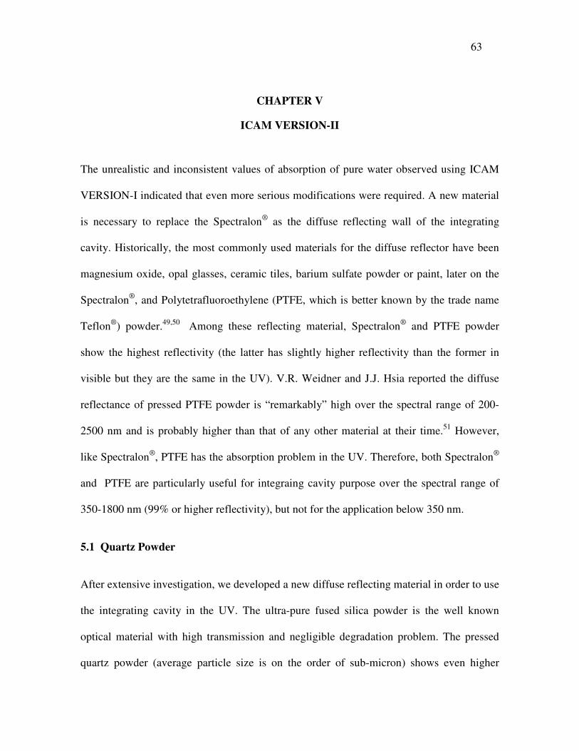
63

CHAPTER V

ICAM VERSION-II

The unrealistic and inconsistent values of absorption of pure water observed using ICAM

VERSION-I indicated that even more serious modifications were required. A new material

is necessary to replace the Spectralon® as the diffuse reflecting wall of the integrating

cavity. Historically, the most commonly used materials for the diffuse reflector have been

magnesium oxide, opal glasses, ceramic tiles, barium sulfate powder or paint, later on the

Spectralon®, and Polytetrafluoroethylene (PTFE, which is better known by the trade name

Teflon®) powder.49,50 Among these reflecting material, Spectralon® and PTFE powder

show the highest reflectivity (the latter has slightly higher reflectivity than the former in

visible but they are the same in the UV). V.R. Weidner and J.J. Hsia reported the diffuse

reflectance of pressed PTFE powder is “remarkably” high over the spectral range of 200-

2500 nm and is probably higher than that of any other material at their time.51 However,

like Spectralon®, PTFE has the absorption problem in the UV. Therefore, both Spectralon®

and PTFE are particularly useful for integraing cavity purpose over the spectral range of

350-1800 nm (99% or higher reflectivity), but not for the application below 350 nm.

5.1 Quartz Powder

After extensive investigation, we developed a new diffuse reflecting material in order to use

the integrating cavity in the UV. The ultra-pure fused silica powder is the well known

optical material with high transmission and negligible degradation problem. The pressed

quartz powder (average particle size is on the order of sub-micron) shows even higher

64

reflectivity (� 99.7%) than Spectralon® in the UV and visible. This high reflectivity is due

to the multiple interface between the quartz particles and surrounding media (e.g., the air).

The pressed quartz powder can be used as diffuse reflector in a wide range of applications.

It can dramatically improve the sensitivity of the integrating cavity absorption meter. It can

be used to build other devices for spectroscopic measurements. Furthermore, its high

reflectivity and negligible degradation lead to potential applications in optical coupling

system (e.g., solid state laser pumped by flash lamp or laser diode).

In this work, the pressed quartz powder was used to build a new inner cavity to replace the

Spectralon® inner cavity in the ICAM VERSION-I. The new instrument was named ICAM

VERSION-II.

5.1.1 Preliminary Test

The reflectance of the pressed quartz powder was experimentally examined by using the

ingegrating cavity technology. Fig. V-1 shows the experimental setup for measuring the

reflectivity of the pressed quartz powder relative to the Spectralon®. A 532 nm laser beam

was aligned to pass through the top and bottom holes on a cubic Spectralon® integrating

cavity with a 8˚ angle off the vertical axis Z. The laser beam was diffusely reflected by the

surface of a Spectralon® block beneath the bottom hole of the cavity. On one side of the

block a portion of the Spectralon® was removed to make a cavity filled by pressed Pegasus

fused silica powder. The pressed powder was flush with the surrounding Spectralon® part.

The diffuse reflected light was collected by the integrating cavity, and then reached the

PMT through a side hole on the cavity after undergoing multiple internal reflections. The

Spectralon® block was mounted on a motor. When the motor was running at a constant

65

speed, the incident laser beam was reflected by the Spectralon® surface and the quartz

powder surface alternately. Therefore the output voltage signal from the PMT was a

modulated signal with varied peak values proportional to the reflectivity of the

corresponding surface. An oscilloscope was used to measure this signal. A neutral density

filter covered the top hole on the cavity to reduce the laser intensity. A Spectralon® screen

Oscilloscope

PMT

Neutral density filter

532 nm laser beam

8˚

Z

Spectralon® block with a cavity filled by quartz powder

Motor

Cubic Spectralon® integrating cavity

Figure V-1. Experimental setup to measure the reflectivity of

quartz powder relative to Spectralon®.

66

was placed inside the integrating cavity to prevent the PMT from “seeing” the directly

reflected light from the Spectralon® without multiple internal reflections.51 The

experimental results shown in Fig. V-2 indicates the reflectivity ratio of the pressed quartz

powder to the Spectralon® is about 1.021.

Quartz powder Spectralon

Figure V-2. Experimental result of measuring the reflectivity of

pressed quartz powder relative to Spectralon® with 532 nm laser and

rotational speed of 1 rev/sec.

67

5.2 New Integrating Cavity Assembly

5.2.1 Configuration

Figure V-3 is the corss section of the ICAM VERSION-II. Compared to the ICAM

VERSION-I, the crucial change is the inner cavity part. The previous Spectralon® inner

cavity was replaced by a fused silica cell. It consists of a TOSOH ED-H synthesized silica

glass wall which is 152 mm long with a 96.5 mm I.D. and a 105 mm O.D.; two end caps

made of TOSOH ES Ground Disc with a 101 mm diameter and a 20 mm diameter center

hole; and two Suprasil 300 fused silica tubes with a 17 mm I.D. and a 20 mm O.D. Each

tube is welded to one end cap. To make a strong connection the bottom cap is welded

together with the cylindrical wall. A 15 mm hole is dirlled at the mid-point of the

cylindrical wall for inserting the output fiber (detecting F0). The quartz sample cell is

embeded in the pressed quartz powder which fills the space between the inner cavity quartz

cell and the sample cell. At both ends of the cavity, the powder is sealed by two

Spectralon® plugs. A modification has been made to the quartz sample cell used in ICAM

VERSION-I. An 8 mm O.D., 2 mm I.D., 2 mm thick fused silica plate is welded to the

sample cell in its mid-point. This small plate is to position the F0 detecting fiber, which is

shielded by a Spectralon® tube.

68

Figure V-3. Cross sections of the integrating cavity assembly

perpendicular to Y axis in the ICAM VERSION-II.

Input fibers

Input fiber

Ferrule

X

Z

Quartz sample cell

Outer cavity wall

F0 detector fiber

Inner cavity quartz cell

Fused silica powder

69

5.2.2 Quartz Powder Handling

The Pegasus fused silica powder was fluffy as it arrived in a glass container. Before it was

put into the cell, the powder was baked to remove the absorbed moisture and the other

organic content. A quartz tube containing the powder was put into an oven whose

temperature was controlled through a transformer. Immediately after the baking process,

the baked quartz powder was filled into the cavity step by step. In each step, a small portion

of quartz powder was added to the cavity using a quartz plate and pressed by a flat end

quartz rod. The entire cavity assembly (including the irradiance F0 detecting fiber shielded

by the Spectralon® tube) was set up in a hood and the specific mask and eye goggles were

required for safety issue. The cavity assembly was mounted on two height adjustable stages

and the sample cell was fixed in the center (along Z axiz) to ensure the thickness of the

pressed powder was uniform. During powder filling process, 4 of the 6 Spectralon® side

wall parts were removed so that we could monitor the pressing process. A flash lamp was

used to introduce the illumination light into the cavity through the inlet tube of the sample

cell after the room light was turned off. With this illumination light we could locate

possible bright spot which indicated a leakage due to a small portion of powder which was

not pressed tightly.

5.3 Absorption Measurement

Absorption measurements started by measuring 4 cavity-empty signal SE, followed by

measuring 4 cavity-full signal SF. The signal difference SF – SE is plotted in Fig. V-4

together with the the signal difference SF – SE result measured by the ICAM VERSION-I.

70

Wavelength (nm)

300 350 400 450 500 550 600

Sf -

Se

0.0

0.1

0.2

0.3

(a)

Wavelength (nm)

300 350 400 450 500 550 600

SF

- SE

0.0

0.2

0.4

0.6

0.8

1.0

1.2

Wavelength (nm)

300 350 400 450 500 550 600

Sf -

Se

0.0

0.1

0.2

0.3

ICAM VERSION-I : SF - SE ICAM VERSION-II : SF - SE

Figure V-4 (a)The difference between the average of 4 cavity-empty signals (SE) and the

average of 4 cavity-full signals (SF) measured by ICAM VERSION-II. (b) Comparison

between ICAM VERSION-I and VERSION-II.

(b)

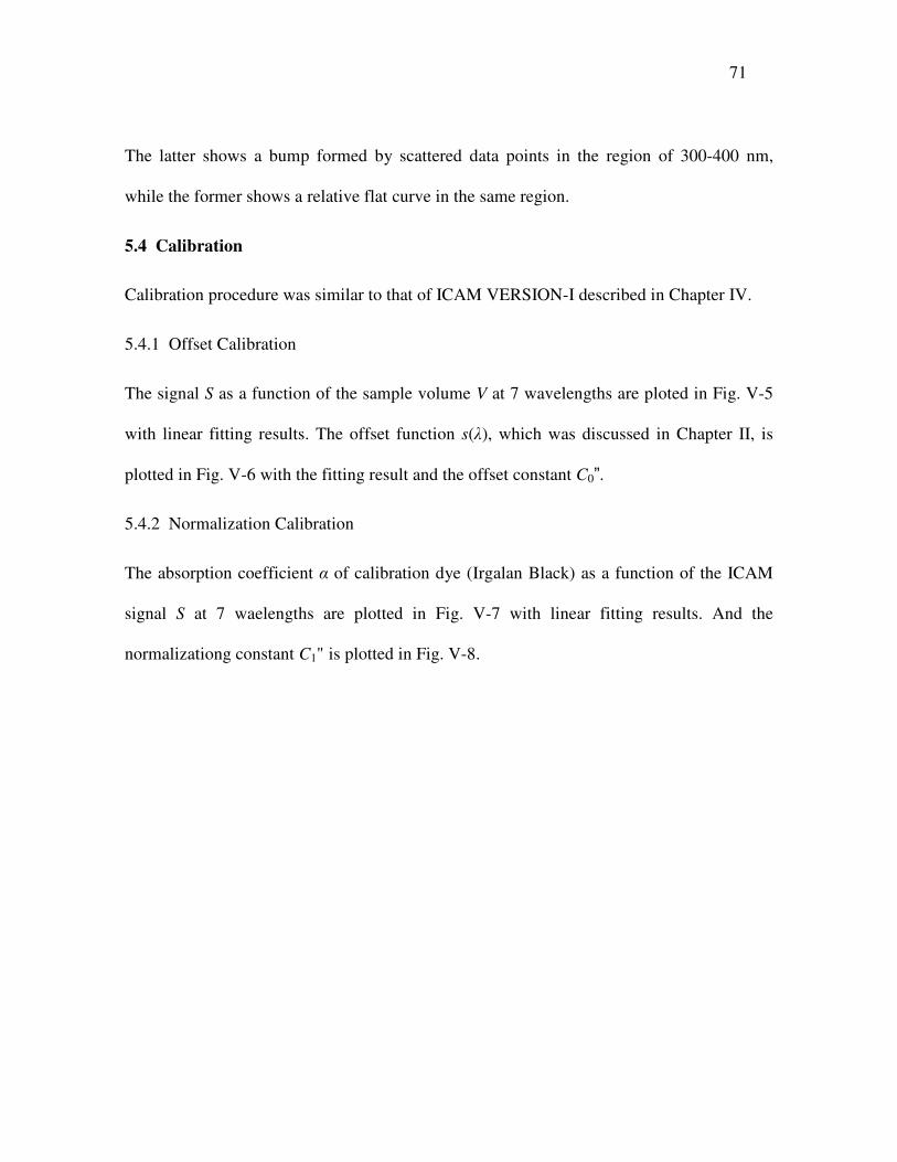
71

The latter shows a bump formed by scattered data points in the region of 300-400 nm,

while the former shows a relative flat curve in the same region.

5.4 Calibration

Calibration procedure was similar to that of ICAM VERSION-I described in Chapter IV.


The signal S as a function of the sample volume V at 7 wavelengths are ploted in Fig. V-5

with linear fitting results. The offset function s(�), which was discussed in Chapter II, is

plotted in Fig. V-6 with the fitting result and the offset constant C0”.


The absorption coefficient � of calibration dye (Irgalan Black) as a function of the ICAM

signal S at 7 waelengths are plotted in Fig. V-7 with linear fitting results. And the

normalizationg constant C1" is plotted in Fig. V-8.

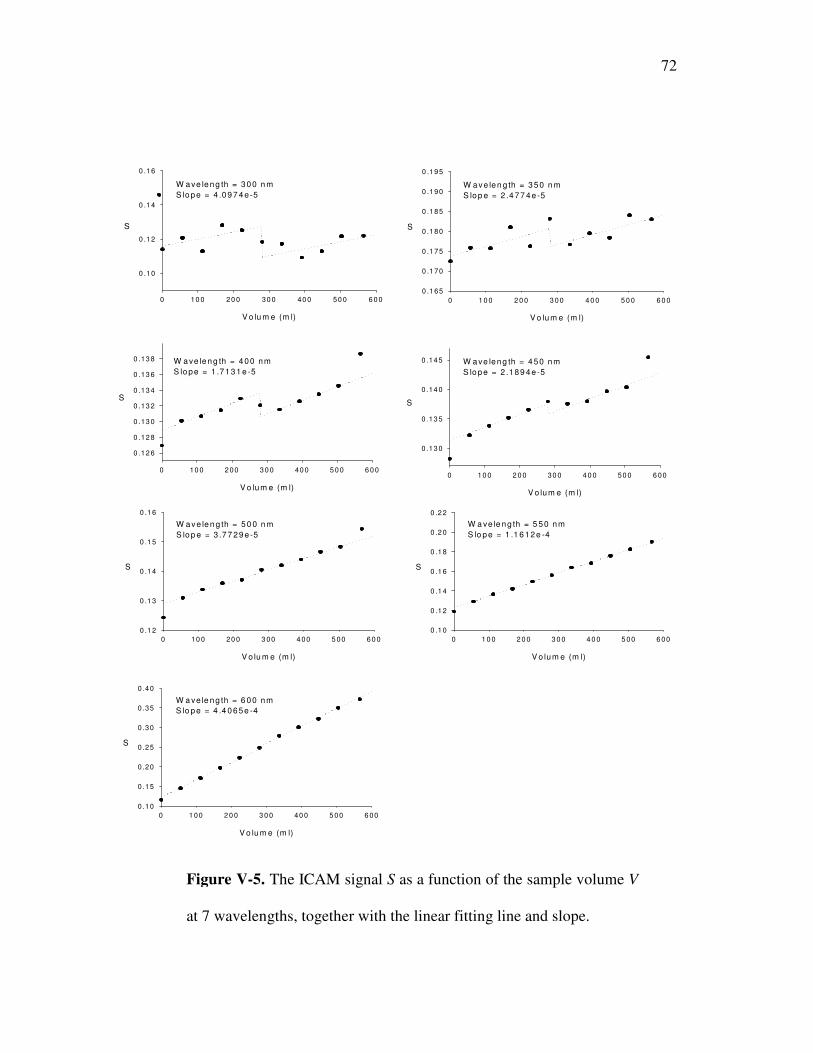
72

V o lu m e (m l)

0 10 0 20 0 30 0 40 0 50 0 6 0 0

S

0 .1 0

0 .1 2

0 .1 4

0 .1 6

W a ve le n g th = 3 0 0 n mS lo p e = 4 .0 9 7 4 e -5

V o lu m e (m l)

0 1 0 0 2 0 0 3 0 0 4 0 0 5 0 0 6 0 0

S

0 .1 65

0 .1 70

0 .1 75

0 .1 80

0 .1 85

0 .1 90

0 .1 95


V o lu m e (m l)

0 10 0 2 00 3 0 0 40 0 5 0 0 6 0 0

S

0 .12 6

0 .12 8

0 .13 0

0 .13 2

0 .13 4

0 .13 6

0 .13 8 W a ve le n g th = 4 0 0 n mS lo p e = 1 .7 1 3 1 e -5

V o lu m e (m l)

0 10 0 2 0 0 30 0 4 0 0 50 0 6 00

S

0 .13 0

0 .13 5

0 .14 0

0 .14 5 W a ve le n g th = 4 5 0 n mS lo p e = 2 .1 8 9 4 e -5

V o lu m e (m l)

0 10 0 20 0 3 00 4 00 5 00 6 0 0

S

0 .1 2

0 .1 3

0 .1 4

0 .1 5

0 .1 6


V o lu m e (m l)

0 1 0 0 2 0 0 3 0 0 4 0 0 5 00 6 00

S

0 .1 0

0 .1 2

0 .1 4

0 .1 6

0 .1 8

0 .2 0

0 .2 2


V o lu m e (m l)

0 1 00 2 0 0 3 0 0 40 0 5 00 6 00

S

0 .10

0 .15

0 .20

0 .25

0 .30

0 .35

0 .40


Figure V-5. The ICAM signal S as a function of the sample volume V

at 7 wavelengths, together with the linear fitting line and slope.

73

Wavelength (nm)

300 350 400 450 500 550 600

S (

λ) a

nd C

o"

-0.06

-0.04

-0.02

0.00

0.02

0.04

0.06

S (λ)Least-square fitting curveOffset constant Co"

Figure V-6. The net offset s(�). The solid curve is the least-square fit

to the data and the dash line is the offset calibration constant C0".

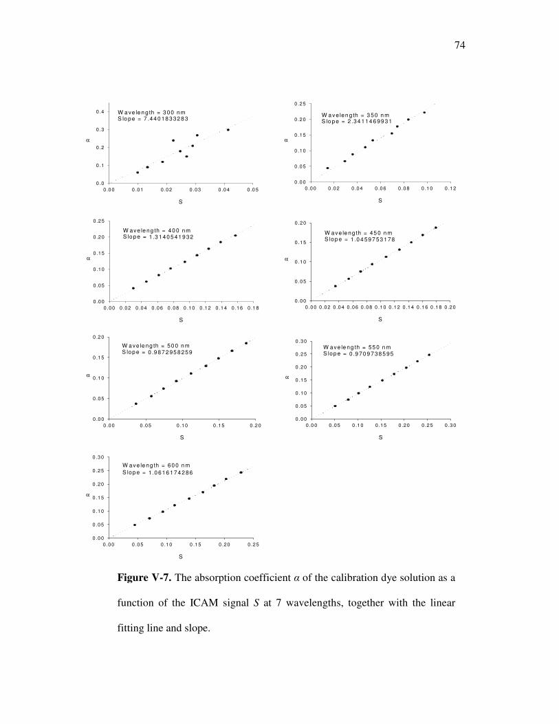
74

S

0 .0 0 0 .0 1 0 .0 2 0 .0 3 0 .0 4 0 .0 5

α

0 .0

0 .1

0 .2

0 .3

0 .4 W a ve le n g th = 3 00 nmS lo pe = 7 .44 0 18 3 32 8 3

S

0 .0 0 0 .0 2 0 .0 4 0 .0 6 0 .0 8 0 .1 0 0 .1 2

α

0 .0 0

0 .0 5

0 .1 0

0 .1 5

0 .2 0

0 .2 5

W a ve len g th = 3 50 n mS lo p e = 2 .34 1 14 6 99 3 1

S

0 .0 0 0 .0 2 0 .0 4 0 .0 6 0 .0 8 0 .1 0 0 .1 2 0 .1 4 0 .1 6 0 .1 8

α

0 .0 0

0 .0 5

0 .1 0

0 .1 5

0 .2 0

0 .2 5

W ave le ng th = 40 0 nmS lop e = 1 .3 1 40 5 41 9 32

S

0 .0 0 0 .0 2 0 .0 4 0 .0 6 0 .0 8 0 .1 0 0 .1 2 0 .1 4 0 .1 6 0 .1 8 0 .2 0

α

0 .0 0

0 .0 5

0 .1 0

0 .1 5

0 .2 0

W ave le ng th = 45 0 n mS lop e = 1 .0 4 59 7 53 1 78

S

0 .0 0 0 .0 5 0 .1 0 0 .1 5 0 .2 0

α

0 .0 0

0 .0 5

0 .1 0

0 .1 5

0 .2 0


S

0 .0 0 0 .0 5 0 .1 0 0 .1 5 0 .2 0 0 .2 5 0 .3 0

α

0 .0 0

0 .0 5

0 .1 0

0 .1 5

0 .2 0

0 .2 5

0 .3 0W ave le ng th = 55 0 n mS lop e = 0 .9 70 9 7 38 5 95

S

0 .0 0 0 .0 5 0 .1 0 0 .1 5 0 .2 0 0 .2 5

α

0 .0 0

0 .0 5

0 .1 0

0 .1 5

0 .2 0

0 .2 5

0 .3 0


Figure V-7. The absorption coefficient � of the calibration dye solution as a

function of the ICAM signal S at 7 wavelengths, together with the linear

fitting line and slope.

75

Wavelength (nm)

300 350 400 450 500 550 600

C1"

0

2

4

6

8

10

Figure V-8. The normalization constant C0” as a function of the wavelength.

76

5.5 Results

The absorption coefficients of pure water in the range of 300-600 nm are plotted in Fig. V-

9. The new data is in good agreement with the work of Pope and Fry10, 22 in the visible

range, as shown in Fig. V-9. It is important to note that these two independent

measurements involve completely different diffuse reflecting wall materials: the pressed

quartz powder and the Spectralon®. Moreover, the experimental set-up and the

measurement procedure are quite different from the previous ICAM: all the optics are UV

compatible; new signal detecting and extracting system is implemented; new sample

generation and sample delivery system are installed; different calibration dye solution is

used; and new data acquisition and instrumental control program is written and used. The

values of the absorption coefficients are listed in Table V-1.

Our new data also supports the work of Sogandares and Fry16, 17. In their experiment, a

different technique using a photothermal probe beam to observe the optical energy

deposited as heat in the water sample was applied. The data was taken in 10-nm steps in the

range of 340-640 nm.

A comparison with the work of other researchers is shown in Fig. V-10. Comparing the

results of Fry’s research group (ICAM VERSION-II data, Pope and Fry data, and

Sogandares and Fry data) with the Tam and Patel data53 and the Smith and Baker data7

shows the significantly lower absorption in the blue. This significant lower absorption in

the blue was confirmed by AMANDA research group in South Pole where the deep sea ice

samples were measured using pulsed laser15. In the UV (300-320 nm) our new data is

77

higher than Quickenden and Irvin data (subtracted the estimation of the Rayleigh scattering

contribution). 18

Table V-1. The absorption coefficients of pure water.

Wavelength (nm)

Absorption coefficient

(m-1)

Wavelength

(nm)


(m-1) 300 0.0504 342 0.0170

302 0.0502 344 0.0161

304 0.0501 346 0.0155

306 0.0467 348 0.0151

308 0.0442 350 0.0150

310 0.0415 352 0.0148

312 0.0388 354 0.0147

314 0.0359 356 0.0145

316 0.0355 358 0.0143

318 0.0354 360 0.0141

320 0.0348 362 0.0141

322 0.0335 364 0.0140

324 0.0325 366 0.0140

326 0.0312 368 0.0140

328 0.0282 370 0.0138

330 0.0256 372 0.0135

332 0.0241 374 0.0136

334 0.0223 376 0.0127

336 0.0208 378 0.0121

338 0.0196 380 0.0115

340 0.0181 382 0.0107

78

Table V-1. Continued.

Wavelength (nm)


(m-1)

Wavelength

(nm)


(m-1) 384 0.0103 434 0.00585

386 0.00985 436 0.00601

388 0.00913 438 0.00614

390 0.00854 440 0.00645

392 0.00830 442 0.00679

394 0.00776 444 0.00725

396 0.00721 446 0.00773

398 0.00715 448 0.00828

400 0.00691 450 0.00880

402 0.00641 452 0.00922

404 0.00623 454 0.00949

406 0.00596 456 0.00971

408 0.00551 458 0.00989

410 0.00524 460 0.0100

412 0.00502 462 0.0100

414 0.00479 464 0.0103

416 0.00483 466 0.0105

418 0.00471 468 0.0107

420 0.00474 470 0.0110

422 0.00495 472 0.0115

424 0.00496 474 0.0117

426 0.00511 476 0.0120

428 0.00530 478 0.0124

430 0.00543 480 0.0129

432 0.00553 482 0.0130

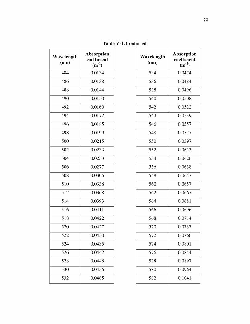
79


Wavelength (nm)


(m-1)

Wavelength

(nm)


(m-1) 484 0.0134 534 0.0474

486 0.0138 536 0.0484

488 0.0144 538 0.0496

490 0.0150 540 0.0508

492 0.0160 542 0.0522

494 0.0172 544 0.0539

496 0.0185 546 0.0557

498 0.0199 548 0.0577

500 0.0215 550 0.0597

502 0.0233 552 0.0613

504 0.0253 554 0.0626

506 0.0277 556 0.0638

508 0.0306 558 0.0647

510 0.0338 560 0.0657

512 0.0368 562 0.0667

514 0.0393 564 0.0681

516 0.0411 566 0.0696

518 0.0422 568 0.0714

520 0.0427 570 0.0737

522 0.0430 572 0.0766

524 0.0435 574 0.0801

526 0.0442 576 0.0844

528 0.0448 578 0.0897

530 0.0456 580 0.0964

532 0.0465 582 0.1041

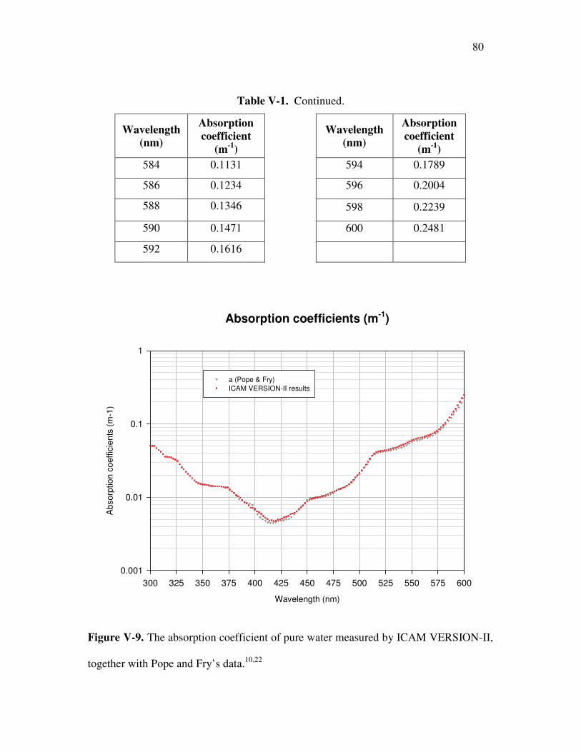
80


Wavelength (nm)


(m-1)

Wavelength

(nm)


(m-1) 584 0.1131 594 0.1789

586 0.1234 596 0.2004

588 0.1346 598 0.2239

590 0.1471 600 0.2481

592 0.1616

Absorption coefficients (m-1)

Wavelength (nm)

300 325 350 375 400 425 450 475 500 525 550 575 600

Abs

orpt

ion

coef

ficie

nts

(m-1

)

0.001

0.01

0.1

1

a (Pope & Fry) ICAM VERSION-II results

Figure V-9. The absorption coefficient of pure water measured by ICAM VERSION-II,

together with Pope and Fry’s data.10,22

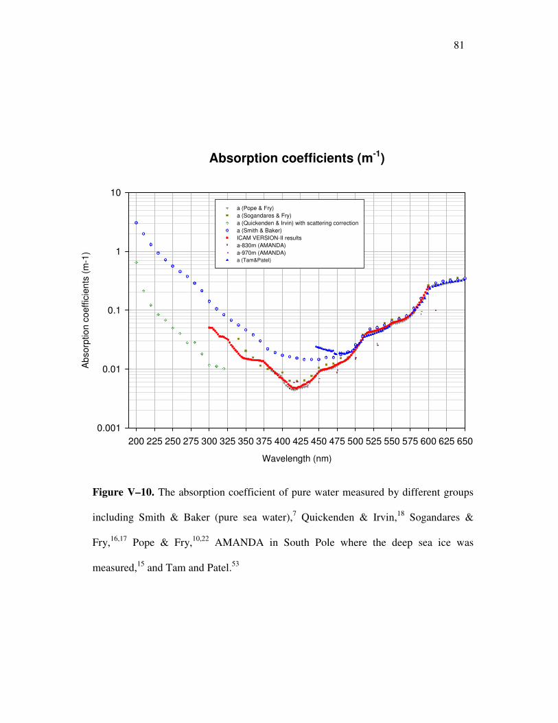
81


Wavelength (nm)

200 225 250 275 300 325 350 375 400 425 450 475 500 525 550 575 600 625 650

Abs

orpt

ion

coef

ficie

nts

(m-1

)

0.001

0.01

0.1

1

10a (Pope & Fry) a (Sogandares & Fry) a (Quickenden & Irvin) with scattering correctiona (Smith & Baker) ICAM VERSION-II resultsa-830m (AMANDA) a-970m (AMANDA) a (Tam&Patel)

Figure V–10. The absorption coefficient of pure water measured by different groups

including Smith & Baker (pure sea water),7 Quickenden & Irvin,18 Sogandares &

Fry,16,17 Pope & Fry,10,22 AMANDA in South Pole where the deep sea ice was

measured,15 and Tam and Patel.53

82

5.6 Resonance Structures

The absorption spectra of pure water identifies the resonance structures (shoulders) due to

the harmonic of O-H stretch mode combined with the fundamental of the scissors mode of

the water molecule.10, 22 Fig. V-11 shows the three fundamental vibrational modes of water

molecule.

The predicated frequencies of the nth harmonic of the O-H stretch mode can be calculated

based on the simple anharmonic formula given by Tam and Patel53:

)1,5(,)633620( 1−−= cmnnnν

Figure V-11. The fundamental vibrational modes of the water molecule.

83

and the frequency of the fundamental scissor mode is 1645 cm-1.

Table V-2 summarizes the vibrational mode assignments with the order of the harmonic of

the O-H stretch mode (v1/v3) and the scissor mode (v2); the positions of some predicated

shoulders and peaks in the absorption spectra of pure water.

Table V-2. Mode assignments with the predicated wavelengths.

Mode assignments

(the order of harmonic)

Predicated shoulder

wavelength

v1 /v3 v2 � (nm)

0 1 6079

1 0 2811

4 0 742

4 1 662

5 0 605

5 1 550

6 0 514

6 1 474

7 0 449

7 1 418

8 0 401

8 1 376

9 0 364

9 1 343

10 0 334

10 1 317

11 0 310

11 1 295

84

Fig. V-12 is another plot of our data to emphasize the resonance structures. Each large

arrow with a boldface integer shows the observed shoulder due to the nth harmonic of the

fundamental O-H stretch mode. Each small arrow with a pair of numbers in parenthesis

shows the minor shoulder due to the conbination modes.

Figure V-12. The ICAM VERSION-II results for the absorption of pure water. A large

arrow with a boldface interger n indicates the position of an oberved shoulder due to the nth

harmonic of the O-H stretch mode; a small arrow with mode assignment (j,1) indicates a

shoulder due to the combination of the jth harmonic of O-H stretch mode with the

fundamental scissors mode.

85

The shoulders that are due to the seventh and eighth harmonics were first observed by

Sogandares and Fry16, 17 and then confirmed by Pope & Fry,10,22. The (7,1) and (6,1) were

first observed by Pope & Fry,10,22 and they have not been readily apparent in water

absorption data of other groups. Our new data confirms these shoulders observed by Fry’s

group in previous work. The (10,1) and (8,1) are two newly observed conbination modes.

5.7 Increased Absorption Due to Long Time Contact of Ultra-pure Water

Pope and Fry22 observed that the long time contact of ultra-pure water with quartz leaded to

significant increased absorption in the blue region. Using ICAM VERSION-II, a fresh pure

water sample was measured and then left in the quartz sample cell. Seven days later the

sample was measured again with the same experimental setting. During the seven days

storage time, the sample was sealed with the high purity nitrogen gas. The measurement

result shown in Fig. V-13. indicates the significant increase of absorption of pure water

stored in quartz for 7 days in both blue and ultraviolet.

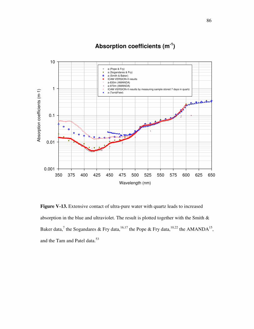
86


Wavelength (nm)

350 375 400 425 450 475 500 525 550 575 600 625 650

Abs

orpt

ion

coef

ficie

nts

(m-1

)

0.001

0.01

0.1

1

10a (Pope & Fry) a (Sogandares & Fry) a (Smith & Baker) ICAM VERSION-II resultsa-830m (AMANDA) a-970m (AMANDA) ICAM VERSION-II results by measuring sample stored 7 days in quartza (Tam&Patel)

Figure V-13. Extensive contact of ultra-pure water with quartz leads to increased

absorption in the blue and ultraviolet. The result is plotted together with the Smith &

Baker data,7 the Sogandares & Fry data,16,17 the Pope & Fry data,10,22 the AMANDA15,

and the Tam and Patel data.53

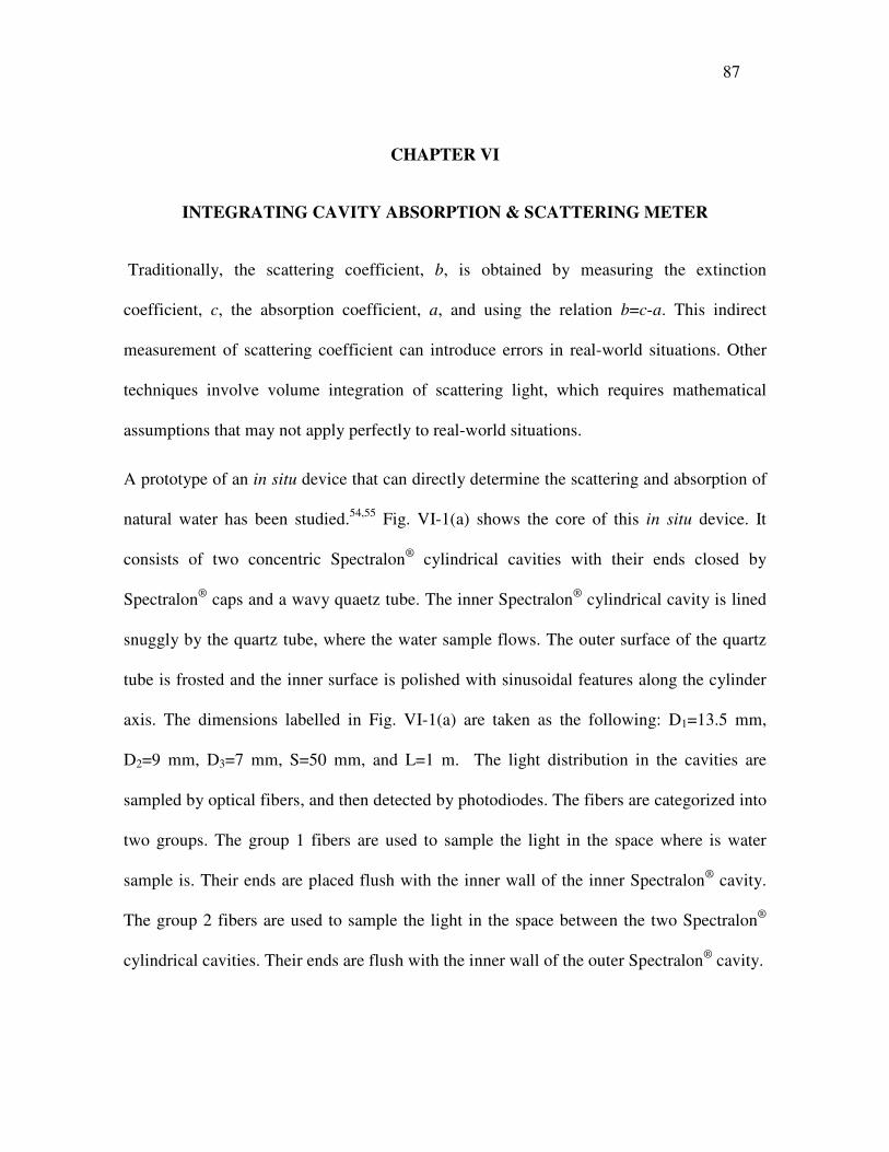
87

CHAPTER VI

INTEGRATING CAVITY ABSORPTION & SCATTERING METER

Traditionally, the scattering coefficient, b, is obtained by measuring the extinction

coefficient, c, the absorption coefficient, a, and using the relation b=c-a. This indirect

measurement of scattering coefficient can introduce errors in real-world situations. Other

techniques involve volume integration of scattering light, which requires mathematical

assumptions that may not apply perfectly to real-world situations.

A prototype of an in situ device that can directly determine the scattering and absorption of

natural water has been studied.54,55 Fig. VI-1(a) shows the core of this in situ device. It

consists of two concentric Spectralon® cylindrical cavities with their ends closed by

Spectralon® caps and a wavy quaetz tube. The inner Spectralon® cylindrical cavity is lined

snuggly by the quartz tube, where the water sample flows. The outer surface of the quartz

tube is frosted and the inner surface is polished with sinusoidal features along the cylinder

axis. The dimensions labelled in Fig. VI-1(a) are taken as the following: D1=13.5 mm,

D2=9 mm, D3=7 mm, S=50 mm, and L=1 m. The light distribution in the cavities are

sampled by optical fibers, and then detected by photodiodes. The fibers are categorized into

two groups. The group 1 fibers are used to sample the light in the space where is water

sample is. Their ends are placed flush with the inner wall of the inner Spectralon® cavity.

The group 2 fibers are used to sample the light in the space between the two Spectralon®

cylindrical cavities. Their ends are flush with the inner wall of the outer Spectralon® cavity.

88

Figure VI-1. Illustration of the in situ device that can directly determine the scattering and

absorption of natural water.

0

89

The introduction of light into the cavity can be achieved in one of the two operating modes:

the Spectralon® illumination mode shown in Fig. VI-1(b) and the end illumination mode

shown in Fig. VI-1(c). The choice of the mode depends on the optical property of the water

to be measured.

To measure the absorption coefficient, the Spectralon® illumination mode is employed. In

this mode, light is guided into the space between the inner and outer cavities through

optical fibers. The slight translucency of the Spectralon® permits some light penetrate

through the wall and enter the space where the quartz tube and the water sample are

located. Due to the highly diffuse reflectance of the Spectralon® wall, the sample is under

the isotropic and homogeneous illumination. The working principle of the device in this

mode is the same as the ICAM VERSION-I and VERSION-II. If absorption is the only

property interested, the wavy quartz tube can be replaced by a smooth quartz tube.

To measure the scattering coefficient, the end illumination mode is employed. A well

collimated light beam (e.g., a laser beam) is sent down the wavy quartz tube into the water

sample along the cylinder axis. It is very important that at no time the beam directly

contacts with the inner surface of the quartz tube. The wavy feature of the quartz tube helps

prevent the scattered light from escaping so that eventually they reach the detecting fibers.

According to the Monte Carlo simulations,54,55 at a distance of around 0.775 m down the

length of cylinder, the detected signal is independent of the g=0 and g=0.97 phase function,

where g is the average cosine of the scattering angle � and phase function is a Henyey-

Greenstein phase function given by

90

)1,6(.cos,)cos21(

141

),( 2/32

2

θθπ

φθ =+−

−= ggg

gp

The g=0 case represents isotropic scattering. The g=0 case is chosen to represent a

“characteristic upper limit” for real ocean water, in this case most of the scattering light

travels forward. The simulation also shows that with a smooth quartz tube, the detected

signals are a lot smaller and very different for different g-parameters. The wavy feature of

the quartz tube is critical for the measurement of the scattering coefficient. Essentially, in

order to measure the scattering coefficient, the best place for the detecting fiber is around

0.775 m from origin shown in Fig. VI-1(a).

The major parts of this in situ device shown in Fiu. VI-1(a) have been built. Each of the two

Spectralon® cylindrical cavities consists of five tubes. An illustration to show how all the

Spectralon® parts are fitted together is shown in Fig. VI-2.

Figure VI-2. An illustration showing how all the Spectralon® parts fit together.

91

Each outer Spectralon® tube is 20 cm long with a 13.5 mm I. D. and a 21.5 mm O. D.. Each

inner Spectralon® tube is 20 cm long with a 32 mm I. D. and a 48 mm O. D.. Each end cap

is 8 mm thick with a 13.5 mm I. D. and a 48 mm O. D..

After the major part of the in situ device was built, we discovered that the Spectralon®

material has absorption and degradation problems. Although the original Spectralon® part is

still useful for the measurements of absorption and scattering in the visible region, it will be

replaced by the pressed quartz powder in the future studies.

92

CHAPTER VII

CONCLUSIONS

The results presented in this dissertation indicate the project objectives were achieved. The

capability of the Integrating Cavity Absoption Meter (ICAM) was significantly improved to

measure the most purified water over the wide spectral range of 300-700 nm. The

absorption measurements confirm the results of Pope and Fry in the visible region,

specifically in the blue (400-450 nm) where the absorption reaches the the minimum.

Besides those resonance structures found in previous work by Sogandares and Pope, some

new shoulders were identified in the ultraviolet. As the newly discovered diffuse

reflectance material, the pressed fused silica powder was applied to replace the most

commonly used Spectralon® material. The integrating cavity based on this new material

overcame the low reflectivities in the UV due to cavity wall absorption. The results in this

work indicate the pressed quartz powder is very useful in diffuse reflectance

spectrophotometry. And it can be used as diffuse reflector for other applications. the fact

that the long time contact of ultra-pure water with quartz leads to a significant increase of

absorption was observed in both the visible and ultraviolet. The major part of an in situ

device that can directly measure the scattering and absorption of the natural water was built

and under the laboratory test.

Limitations of the current ICAM include the time-consuming calibration process and the

corresponding data analysis. New technique based on integrating cavity theory with no (or

minimized) calibration efforts will be particularly useful. For example: Fry pointed out that

93

by measuring the output signal from an empty integrating cavity (made by pressed quartz

powder) in response to a very short (in nano-second level) input laser pulse, and comparing

the result to the case where the cavity is filled with pure water, it is possible to extract the

water absorption information from the laser pulse broading time.

As this dissertation is written, the construction of a new integrating cavity (ICAM

VERSION-III) is underway. A smaller quartz sample cell will replace the previous cell so

that the quartz powder filling the space between the inner cavity cell and the sample cell

will be thicker (currently the thickness of the pressed powder is 5 mm, and it will be

increased to 16 mm thickness). This time the powder will be baked overnight together with

the inner cavity quartz cell. They will be sealed inside a stainless steel vacuum chamber to

prevent the possible contaminants from the oven. During the baking process, a sorption

pump will be used to remove the moisture and other organic contaminats in the quartz

powder. Once the baking process is completed, the vacuum chamber will be filled with the

high purity nitrogen gas.

94

REFERENCES

[1] A. Morel, “Optical properties of oceanic Case 1 waters. Revisited,” in Ocean Optics

XIII, S.G. Ackleson and R.Frouin, eds., Proc. SPIE 2963, 108-114 (1997).

[2] K. K. Voss, “A spectral model of the beam attenuation coefficient in the ocean and

coastal areas,” Limnol. Oceanogr. 37, 501 (1992).

[3] A. Morel, “Light and marine photosynthesis: A spectral model with geochemical and

climatological implications,” Prog. Oceanogr. 26, 263 (1991).

[4] R. M. Pope, A. D. Weidemann. And E. S. Fry, “Integrating cavity absorption meter

measurements of dissolved substances and suspended particles in ocean water,” Dynamics

of Atmospheres and Oceans 31, 307-320 (2000).

[5] H. Buiteveld, J. H. M. Hakvoort, and M. Donze, “The optical properties of pure water,”

in Ocean Optics XII, J. S. Jaffe, ed., Proc. SPIE 2258, 174-183 (1994)

[6] M. R. Querry, D. M. Wieliczka, and D. J. Segelstein, “Water (H2O),” in Handbook of

Optical Constants of Solids II, E. D. Palik, ed., (Academic Press, Inc., Boston, 1991) pp.

1059-1077.

[7] R. C. Smith and K. S. Baker, “Optical properties of the clearest natural waters (200-800

nm),” Appl. Opt. 20, 177-184 (1981).

[8] W. M. Irvine and J. B. Pollack, “Infrared optical properties of water and ice spheres,”

ICARUS 8, 324-360 (1968).

[9] C. D. Mobley, “The optical properties of water,” in Handbook of Optics, M. Bass, ed.,

(McGraw-Hill, New York, 1995) pp. 43.3-43.56.

95

[10] R. M. Pope and E. S. Fry, “Absorption spectrum (380-700 nm) of pure water: II,

Integrating cavity measurements,” Appl. Opt. 36, 8710-8723 (1997).

[11] E. S. Fry and G. W. Kattawar, “Measurement of the absorption coefficient of ocean

water using isotropic illumination,” in Ocean Optics IX, M.A. Blizard, ed., Proc. SPIE 925,

142-148 (1988).

[12] E. S. Fry, G. W. Kattawar, and R. M. Pope, “Integrating cavity absorption meter,”

Appl. Opt. 31, 2055-2065 (1992).

[13] E. S. Fry, “Visible and near-ultraviolet absorption spectrum of liquid water:

comment’” Appl Opt. 39, 2743-2744 (2000).

[14] E. S. Fry, “Reply to criticisms of the Pope and Fry paper on pure water absorption

made in a comment by Quickenden et al.,” Appl. Opt. 39, 5843-5846 (2000).

[15] AMANDA Collaboration, “ Optical properties of deep sea ice at the South Pole:

absorption,” Appl. Opt. 38, 4168-4180 (1997).

[16] F. M. Sogandares and E. S. Fry, “Absorption spectrum (340-640 nm) of pure water: I.

Photothermal measurements,” Appl Opt. 36, 8699-8709 (1997).

[17] F. M. Sogandares, “The spectral absorption of pure watrer,” Ph. D. dissertation (Texas

A&M University, College Station, 1991).

[18] T. I. Quickenden and J. A. Irvin, “the ultraviolet absorption spectrum of liquid water,”

J. Chem Phys. 72, 4416-4428 (1980).

[19] R. A. J. Litjens, T. I. Quickenden, and C. G. Freeman, “Visible and near-ultraviolet

absorption spectrum of liquid water,” Appl. Opt. 38, 1216-1223 (1999).

[20] P. Elterman, “Integrating cavity spectroscopy,” Appl. Opt. 9, 2140-2142 (1970)

96

[21] J. T. O. Kirk, “Modeling the performance of an integrating-cavity absorption meter:

theory and calculations for a spherical cavity,” Appl. Opt. 34, 4397-4408 (1995).

[22] R. M. Pope, “Optical absorption of pure water and sea water using the integrating

cavity absorption meter,” Ph.D. dissertation (Texas A&M University, College Station,

1993).

[23] L. Cui, “Improved integrating cavity absorption meter,” M.S. thesis (Texas A&M

University, College Station, 2000).

[24] Millipore Corporation, A10 Brochure, Bedford, Mass., 1996.

[25] J. G. Calvert and J. N. Pitts, Photochemistry (Wiley, New York, 1966)

[26] High-Q, Inc, Reagent-Grade Water Newsletter, issue #0201, (High-Q, Inc., Wilmette,

IL., 2002).

[27] Millipore Corporation, Operating and Maintenance Manual, (Millipore Corp.,

Bedford, Mass., 2001).

[28] A. Preece, A Manual for Histologic Technicians, 3rd ed., (Little, Brown & Co.,

Boston, 1972) pp. 27.

[29] J. Crookham, R. Dapson , Hazardous Chemicals in the Histopathology Laboratory,

2nd ed., (Anatech Ltd., Denver, NC., 1991).

[30] Oriel Instruments, The Book of Photon Tools, (Oriel Instruments, Stratford, Conn.,

2002).

[31] CVI Laser Corporation, 2004 Catalog, (CVI Laser Corp., Albuquerque, N.M., 2004).

[32] CVI Laser Corporation, DIGIKROM 240 Instruction Manual, (CVI Laser Corp.,

Albuquerque, N.M., 1988).

97

[33] CVI Technical Service (800-296-9541), (personal communication, January. 2002).

[34] Labsphere, Inc., A Guide to Reflectance Coatings and Materials, (Labsphere, Inc.,

North Sutton, N. H., 2004).

[35] Labsphere, Inc., Spectralon® Product Data Sheet, (Labsphere, Inc., North Sutton, N.

H., 2001).

[36] Joan G. Demers, Sr. Technical Sales Representative, (Labsphere, Inc., North Sutton,

N. H.) (facsimile transmission 5 May 1989).

[37] EG&G Instruments, Precision Light Chopper Model 197 User Manual, (Princeton

Applied Research, Oak Ridge, TN, 1999).

[38] Stanford Research System, SR830 Lock-In Amplifier Operating Manual and

Programming Reference, (Sunnyale, CA, 1999).

[39] EG&G Instruments, Model 5210 Lock-in Amplifier Instruction Manual, (Princeton

Applied Research, Oak Ridge, TN, 1989).

[40] Life in the Atacama 2005 Science/Technology Workshop, NASA Ames Research

Center / Carnegie Mellon, Pittsburgh, PA, 2005.

[41] X. Zhao, Z. Lu and E. S. Fry, “Absorption spectrum (300-700 nm) of pure water using

an integrating cavity absorption meter,” in Ocean Optics XVI, available on CD. from Office

of Naval Research, Ocean, Atmosphere, and Space S&T Department, Arlington, VA

(2002).

[42] E. S. Fry, Z. Lu, X. Zhao and X. Qu, “Absorption of pure warter in the 300-400 nm

range,” in Ocean Optics XVII, available on CD. from Office of Naval Research, Ocean,

Atmosphere, and Space S&T Department, Arlington, VA (2004).

98

[43] A. E. Stiegmann, C. J. Bruegge and A. W. Springsteen, “Ultraviolet stability and

contamination analysis of Spectralon diffuse reflectance material,” Opt. Eng. 32, 799-804

(1993).

[44] D. R. Gibbs, F. J. Duncan and T. M. Goodman, “Ageing of materials under intense

ultraviolet radiation,” Metrologia 32 601-607, (1996).

[45] C. J. Bruegge, A. E. Stiegmann, R. A. Rainen and A. W. Springsteen, “Use of

Spectralon as a diffuse reflectance standard for in-flight calibration of earth-orbiting

sensors,” Opt. Eng. 32, 805-814 (1993).

[46] E. Hilsenrath, H. Herzig, D. E. Williams, C. J. Bruegge and A. E. Stiegman, “Effects

of space shuttle flight on the reflectance characteristics of diffusers in the near-infrared,

visible, and ultraviolet regions,” Opt. Eng. 33, 3675-3681 (1994).

[47] P. C. Knee, “Investigation of the uniformity and ageing of integrating spheres,” Anal.

Chim. Acta 380, 391-399 (1999).

[48] W MÖller, K-P Nikolaus and A. HÖpe, “Degradation of the diffuse reflectance of

Spectralon under low-level irradiation,” Metrologia 40, S212-S215 (2003).

[49] Bureau Central de la Commission Internationale de l’Eclairage, Review of Publications

on Properties and Reflection Values of Material Reflection Standards, (CIE Publication 46

(TC-2.3), Paris, 1979) pp. 15-72.

[50] Dr. Gröbel UV-Elektronik GmbH, Product Catalog, (Ettlingen, Deutschland, 1980).

[51] V. R. Weidner and J. J. Hsia, “Reflection properties of pressed Polytetrafluoroethylene

powder“, J. Opt. Soc. Am. 71, 856-861 (1981).

99

[52] Labsphere, Inc., A Guide to Ingegrating Sphere Radiometry and Photometry,

(Labsphere, Inc., North Sutton, N. H., 2001).

[53] A. C. Tam and C. K. N. Patel, “ Optical absorption of light and heavy water by laser

optoacoustic spectroscopy,” Appl. Opt. 18, 3348-3358 (1979).

[54] D. J. Gray, G. W. Kattawar, E. S. Fry, and X. Zhao, “Theoretical analysis of a novel

in situ scattering and absorption meter,” in Ocean Optics XVI, available on CD. from Office

of Naval Research, Ocean, Atmosphere, and Space S&T Department, Arlington, VA

(2002).

[55] E. S. Fry, G. W. Kattawar, D. J. Gray, X. Zhao, and Z. Lu, “Apparatus and method for

direct measurement of absorption and scattering coefficient in situ,” U. S. patent

20040141179A1 (2004).

100

VITA

Zheng Lu was born in Taiyuan, Shanxi, P.R. China in 1973, to Zhaoying Du and Xingshu

Lu. He graduated from the Shandong University in 1996 with a B.S. degree in Optics. In

July of 1999 he completed a M.S. degree in Optics from the Institute of Modern Optics at

Nankai University. He married Xinmei Qu on 26 July, 1999 and then they came to the

United States. They have enjoyed study and research work as graduate students at Texas

A&M University. He received his Ph.D. degree in Physics from Texas A&M University in

May 2006. His permanent address is 3 Tianwaicun Street, Taishan Sanatorium, Taian,

Shandong 271000, P.R.China.

Documents

OPTICAL ABSORPTION OF PURE WATER IN THE BLUE AND …