Embed Size (px)
DESCRIPTION
Opinionated. Lessons. in Statistics. by Bill Press. #15.5 Poisson Processes and Order Statistics. Professor William H. Press, Department of Computer Science, the University of Texas at Austin. - PowerPoint PPT Presentation
Citation preview
1
Opinionated
in Statisticsby Bill Press
Lessons
#15.5 Poisson Processes and Order Statistics
Professor William H. Press, Department of Computer Science, the University of Texas at Austin

In a “constant rate Poisson process”, independent events occur with a constant probability per unit time
In any small interval t, the probability of an event is t
In any finite interval , the mean (expected) number of events is
2

What is the probability distribution of the waiting time to the 1st event, or between events?
It’s the product of t/t “didn’t occur” probabilities, times one “did occur” probability.
(random variable T1 with value t)
Get it? It’s the probability that 0 events occurred in a Poisson distribution with t mean events up to time t, times the probability (density) of one event occurring at time t. 3
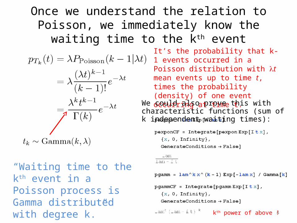
Once we understand the relation to Poisson, we immediately know the waiting time to the kth event
It’s the probability that k-1 events occurred in a Poisson distribution with t mean events up to time t, times the probability (density) of one event occurring at time t.
“Waiting time to the kth event in a Poisson process is Gamma distributed with degree k.”
We could also prove this with characteristic functions (sum of k independent waiting times):
kth power of above ! 4

Same ideas go through for a “variable rate Poisson process”
where
5
Waiting time to first event or between events:
so basically the area (t) replaces the area t
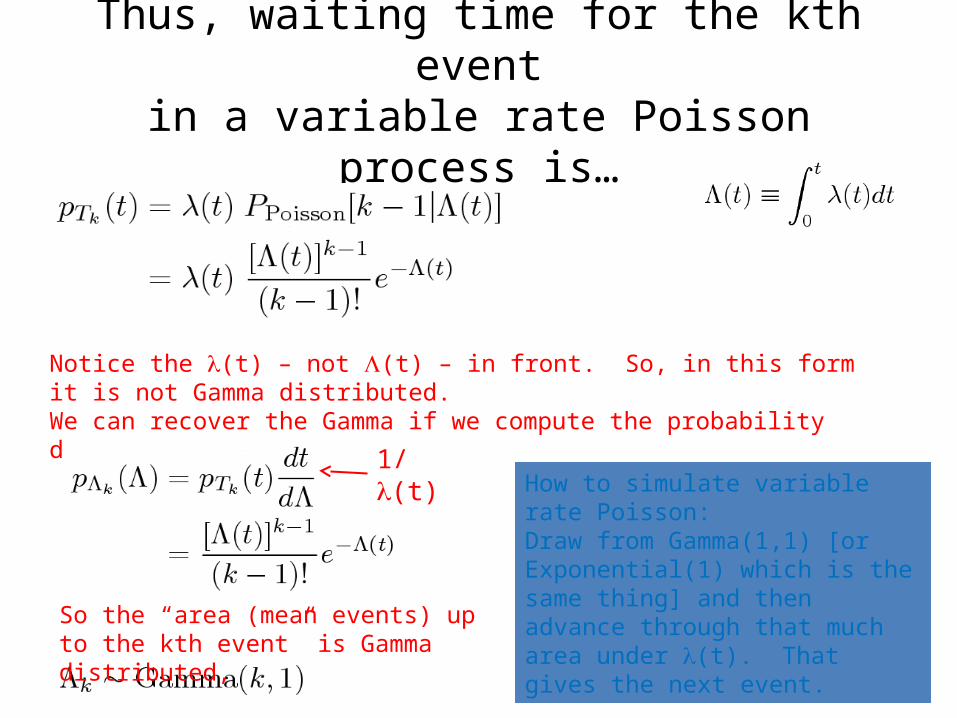
Thus, waiting time for the kth eventin a variable rate Poisson process is…
6
Notice the (t) – not (t) – in front. So, in this form it is not Gamma distributed.We can recover the Gamma if we compute the probability density of (t)
1/(t)
So the “area (mean events) up to the kth event” is Gamma distributed,
How to simulate variable rate Poisson:Draw from Gamma(1,1) [or Exponential(1) which is the same thing] and then advance through that much area under (t). That gives the next event.
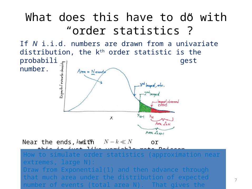
What does this have to do with “order statistics”?
7
If N i.i.d. numbers are drawn from a univariate distribution, the kth order statistic is the probability distribution of the kth largest number.
Near the ends, with or , this is just like variable-rate Poisson. How to simulate order statistics (approximation near extremes, large N):Draw from Exponential(1) and then advance through that much area under the distribution of expected number of events (total area N). That gives the next event.
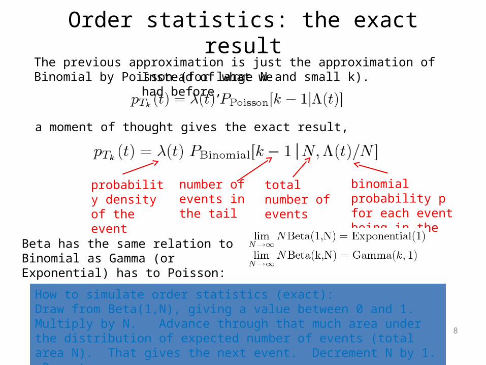
Order statistics: the exact result
8
The previous approximation is just the approximation of Binomial by Poisson (for large N and small k).
a moment of thought gives the exact result,
binomial probability p for each event being in the tail
number of events in the tail
probability density of the event
total number of events
How to simulate order statistics (exact):Draw from Beta(1,N), giving a value between 0 and 1. Multiply by N. Advance through that much area under the distribution of expected number of events (total area N). That gives the next event. Decrement N by 1. Repeat.
Beta has the same relation to Binomial as Gamma (or Exponential) has to Poisson:
Instead of what we had before,