Embed Size (px)
Citation preview

Postal Regulatory CommissionSubmitted 2/26/2007 10:47 amFiling ID: 55901
United States of AmericaPOSTAL REGULATORY COMMISSION
Before:
Chairman Blair,Vice Chairman Tisdale,
Commissioners Acton, Goldway and Hammond
OPINION
AND
RECOMMENDED DECISION
VOLUME 2
Washington, DC 20268-0001February 26, 2007
Postal Rate and Fee Changes Docket No. R2006-1
Accepted 2/26/2007


APPENDICESTABLE OF CONTENTS
APPENDIX A
PARTICIPANTS AND COUNSEL OR REPRESENTATIVE
APPENDIX B
WITNESSES’ TESTIMONY
APPENDIX C
REVENUE REQUIREMENT FOR TEST YEAR WITH PROPOSED REVENUE AND COSTS
APPENDIX D
DEVELOPMENT OF REVENUE REQUIREMENT AND COST ROLL FORWARD CORRECTIONS
a Revisions to Revenues, Costs, and Final Adjustments ........................... 1
1 Postal Service Revisions ................................................................ 1(a) Revenues ............................................................................... 2(b) Costs ...................................................................................... 2
2 Commission Corrections ................................................................. 2(a) Base Year Periodicals Costs in Cost Segment 6 ................... 2(b) Final Adjustments Corrections ............................................... 3(c) Summary ................................................................................ 4
b Adjustments to Postal Service Compensation and Benefits Cost Factors for Known and Certain Events ...................................................................... 4
1 Adjustments Due to CPI-W Actual Results ..................................... 52 Adjustments Due to Actual Health Benefits Increases ................... 63 Other Changes to Compensation and Benefits Cost Levels .......... 64 Adjustments to Cost Reductions and Other Programs ................... 75 Summary ........................................................................................ 7
c Other Revenue Requirement Adjustments .............................................. 8
d Implementation of the Commission’s Cost Attribution Methodologies and Revenue Requirement Changes ............................................................. 8
i of iii

Docket No. R2006-1
APPENDIX E
COMPARISON OF COSTS ATTRIBUTED BY COST SEGMENT AND COMPONENT
APPENDIX F
PRC DISTRIBUTION OF ATTRIBUTABLE COSTS TO CLASSES AND SUBCLASSES
APPENDIX G
TEST YEAR VOLUME, COST, REVENUE, AND COST COVERAGE BY CLASS
APPENDIX H
COMPARISON OF ESTIMATED TEST YEAR VOLUMES
APPENDIX I
ECONOMIC DEMAND MODELS AND FORECAST METHODOLOGY
APPENDIX J
MAIL PROCESSING VARIABILITY
1 Summary ........................................................................................ 12 Positions of the Participants ........................................................... 3
(a) The Postal Service’s Revised Mail Processing Model ........... 3(b) The Research Sponsored by the OCA ................................... 7
(1)Roberts’ 2002 Paper .......................................................... 7(2)Roberts’ March 2006 Paper ............................................. 13(3)Roberts’ Testimony .......................................................... 16
(c) Witness Neels’ Testimony .................................................... 18(d) Witness Haldi’s Testimony ................................................... 24(e) Witness Elliott’s Testimony .................................................. 28(f) Witness Oronzio’s Testimony ............................................... 30
ii of iii

APPENDICES
3 Commission Analysis .................................................................... 31(a) The Theoretical Debate ........................................................ 31
(1)Definition of “Output” ........................................................ 32(2)Endogeneity, Separability, and Proportionality ................ 40
(b) Technical Issues .................................................................. 45(1)Data Quality ..................................................................... 45(2)Correcting for errors in the MODS data. .......................... 55(3)Augmented Commission method. .................................... 77
(c) Seasonal effects. .................................................................. 82(d) Reasonableness of the Model Results. ................................ 86
APPENDIX K
DESCRIPTION OF NEWLY AVAILABLE CARRIER STREET TIME DATA
APPENDIX L
CHALLENGES IN APPLYING INSTRUMENTAL VARIABLES PROCEDURES TO ESTIMATE MAIL PROCESSING VARIABILITIES
iii of iii


Appendix APARTICIPANTS AND COUNSEL OR REPRESENTATIVE
Advo Inc. (Advo)John M. BurzioThomas W. McLaughlin
Alliance of Independent Store Owners and Professionals (AISOP)*Donna E. Hanbery
Alliance of Nonprofit Mailers (ANM)David M. LevyRichard E. Young
Amazon.com, Inc.William J. OlsonJohn S. MilesJeremiah L. Morgan
American Bankers Association (ABA)Gregory F. Taylor
American Bankers Association and National Association of Presort Mailers (ABA-NAPM)Gregory F. TaylorRobert J. BrinkmannIrving D. WardenDavid M. LevyPaul A. Kemnitzer
American Business Media (ABM)David R. Straus
American Postal Workers Union, AFL-CIO (APWU)Darryl J. AndersonJennifer L. Wood
Association for Mail Electronic Enhancement (AMEE)*John A. Sexton
Association for Postal Commerce (PostCom)Ian D. VolnerRita L. BrickmanJennifer T. Mallon
1 of 6

Docket No. R2006-1
Association of Alternate Postal Systems (AAPS)*David R. StrausBonnie S. Blair
Association of American Publishers (AAP)John R. PrzypysznyPhilip J. Mause
Association of Priority Mail Users, Inc. (APMU)William J. OlsonJohn S. MilesJeremiah L. Morgan
Bank of America Corporation (BAC)David M. Levy
Banta Corporation (Banta)*Thomas K. Murray
Douglas F. Carlson (Carlson)*Douglas F. Carlson
Center for Study of Responsive Law*Christopher Shaw
Condè Nast Publications, Inc. (Condè Nast)*Howard Schwartz
Continuity Shippers Association (CSA)Aaron Horowitz
DHL GlobalmailGerard Hempstead
DigiStamp, Inc. (DigiStamp)*Rick Borgers
Direct Marketing Association, Inc. (DMA)Dana T. Ackerly II
2 of 6
* Limited Participant

Discover Financial Services LLC & Morgan Stanley, Inc. (DFS & Morgan Stanley)Robert J. BrinkmannIrving Warden
District Photo, Inc. (District Photo)William J. OlsonJohn S. MilesJeremiah L. Morgan
DMA Nonprofit Federation (DMANF)Senny Boone
Dow Jones & Company, Inc. (Dow Jones)Michael F. McBrideBruce W. NeelyT. Randolph McEvoy
DST Mailing Services, Inc. (DST)*Michael W. Hall
Financial Services Roundtable (FSR)Richard M. Whiting
Flute Network, TheJanyce S. Pritchard
GrayHair Software, Inc.Cameron Bellamy
Greeting Card Association (GCA)James HorwoodDavid Stover
Growing Family, Inc. (Growing Family)*David R. Straus
HSBC North America Holdings, Inc. (HSBC)Jeffrey S. Berlin
Magazine Publishers of America, Inc. (MPA)David M. LevyPaul A. Kemnitzer
3 of 6

Docket No. R2006-1
Mail Order Association of America (MOAA)David C. Todd
Mailing & Fulfillment Service Association (MFSA)Ian D. VolnerRita L. BrickmanJennifer T. Mallon
Major Mailers Association (MMA)Michael W. Hall
MBI, Inc. (MBI)Lynn E. ZimmermannMichael Wilbur
McGraw-Hill Companies, Inc., The (McGraw-Hill)Timothy W. Bergin
National Association of Postmasters of the United States (NAPUS)*Robert M. Levi
National Association of Presort Mailers (NAPM)David M. LevyPaul A. Kemnitzer
National Newspaper Association (NNA)Tonda F. Rush
National Postal Mail Handlers Union (NPMHU)*Bruce R. Lerner
National Postal Policy Council (NPPC)David M. LevyRichard E. YoungPaul A. Kemnitzer
Newspaper Association of America (NAA)William B. Baker
4 of 6
* Limited Participant

Office of the Consumer Advocate (OCA)Shelley S. DreifussEmmitt Rand Costich
Kenneth E. Richardson
Parcel Shippers Association (PSA)Timothy J. May
Pitney Bowes Inc. (Pitney Bowes)James Pierce MyersMichael F. Scanlon
David B. Popkin (Popkin)*David B. Popkin
Quad/Graphics, Inc. (Quad)*Andrew R. SchieslJoe Schick
Return Mail, Inc. (RMI)R. Mitchell HungerpillerT. Alan Ritchie
R. R. Donnelley & Sons Company (Donnelley)*Ian D. VolnerRita L. BrickmanJennifer T. Mallon
Saturation Mailers CoalitionJohn M. BurzioThomas W. McLaughlinDonna E. Hanbery
Time Warner Inc. (Time Warner)John M. BurzioTimothy L. Keegan
United Parcel Service (UPS)John E. McKeeverPhillip E. Wilson, Jr.Laura A. Biancke
5 of 6

Docket No. R2006-1
United States Postal Service (Postal Service)Daniel J. Foucheaux, Jr.Frank R. HeseltonKenneth N. HolliesEric P. KoettingNan K. McKenzieSheela A. PortonovoElizabeth ReedBrian M. ReimerScott L. ReiterDavid H. RubinMichael T. TidwellKeith E. Weidner
U.S. News & World Report, L.P. (U.S. News)*Peter Dwoskin
Valpak Dealers’ Association, Inc. (VPDA)1
William J. OlsonJohn S. MilesJeremiah L. Morgan
Valpak Direct Marketing Systems, Inc. (VDMS)†
William J. OlsonJohn S. MilesJeremiah L. Morgan
Washington Mutual BankTimothy J. May
Karl Wesner (Wesner)*Karl Wesner
1 Valpak Dealers’ Association, Inc. (VPDA) and Valpak Direct Marketing Systems, Inc. (VDMS) are collectively referred to herein as Valpak.
* Limited Participant
6 of 6

Appendix B
WITNESSES’ TESTIMONY
Abdirahman, Abdulkadir M. Postal Service USPS-T-22Postal Service USPS-RT-7
Angelides, Peter A., Ph.D. Association for Postal Commerce and Mailing & Fulfillment Service Association
PostCom-T-4
Association for Postal Commerce and Mailing & Fulfillment Service Association
PostCom-T-5
Bell, Elizabeth A. National Association of Presort Mailers NAPM-RT-1Bellamy, Cameron GrayHair Software GHS-T-1
GrayHair Software GHS-ST-1Bentley, Richard E. Major Mailers Association, DST Mailing
Services, Inc., and Association for Mail Electronic Enhancement
MMA-T-1
Berkeley, Susan W. Postal Service USPS-T-34Postal Service USPS-T-39Postal Service USPS-RT-17
Bernstein, Peter Postal Service USPS-T-8Bozzo, A. Thomas Postal Service USPS-T-12
Postal Service USPS-T-46Postal Service USPS-RT-1Postal Service USPS-RT-5
Bradfield, Lou American Business Media ABM-RT-1Bradley, Michael D. Postal Service USPS-T-14
Postal Service USPS-T-17Postal Service USPS-RT-4
Buc, Lawrence G. Direct Marketing Association, Inc. DMA-T-1Direct Marketing Association, Inc. DMA-RT-1Pitney Bowes Inc. PB-T-2Pitney Bowes Inc. PB-T-3
Callow, James F. Office of the Consumer Advocate OCA-T-5Carlson, Douglas F. Douglas F. Carlson DFC-T-1Cavnar, Nicholas American Business Media ABM-T-1Clifton, James A. American Bankers Association, and National
Association of Presort MailersABA-NAPM-T-1
Greeting Card Association GCA-T-1Cohen, Rita D. Magazine Publishers of America, Inc., and
Alliance of Nonprofit MailersMPA/ANM-T-1
1 of 5

Docket No. R2006-1
Coombs, Joyce K. Postal Service USPS-T-44Crowder, Antoinette Magazine Publishers of America, Inc., et al.1 MPA et al.-RT-1
Saturation Mailers Coalition, and Advo, Inc. SMC-RT-1Cutting, Samuel T. Postal Service USPS-T-26Czigler, Martin Postal Service USPS-T-1Davis, Scott J. Postal Service USPS-T-47Elliott, Stuart W. Magazine Publishers of America, Inc., et al.2 MPA et al.-RT-2
Finley, Chris Parcel Shippers Association PSA-T-1Geddes, R. Richard United Parcel Service UPS-T-3Glick, Sander A. Magazine Publishers Association, and
Alliance of Nonprofit MailersMPA/ANM-T-2
Parcel Shippers Association PSA-RT-1Parcel Shippers Association, Association for Postal Commerce, and Mailing & Fulfillment Service Association
PSA/PostCom-T-1
Association for Postal Commerce, and Mailing & Fulfillment Service Association
PostCom-T-1
Gorham, David Major Mailers Association MMA-RT-2Gorman, Pete Saturation Mailers Coalition SMC-T-1Haldi, John, Ph.D. Amazon.com, Inc. AMZ-T-1
Valpak3 VP-T-2
Harahush, Thomas W. Postal Service USPS-T-4Heath, Max National Newspaper Association NNA-T-1Hintenach, Frederick J., III Postal Service USPS-T-43Horowitz, Aaron Association for Postal Commerce, et al.4 PostCom-T-6
Hunter, Herbert B., III Postal Service USPS-T-2Ingraham, Allan T. Newspaper Association of America NAA-T-2
Newspaper Association of America NAA-RT-2Kaneer, Kirk T. Postal Service USPS-T-41Kelejian, Harry Greeting Card Association GCA-T-5Kelley, John P. Postal Service USPS-T-15
Postal Service USPS-T-30Postal Service USPS-RT-6
2 of 5
1 Magazine Publishers of America, Inc., Advo, Inc., Alliance of Nonprofit Mailers, American Business Media, Dow Jones & Co., The McGraw-Hill Companies, Inc., Mail Order Association of America, National Newspaper Association, Saturation Mailers Coalition, and Time Warner Inc.
2 Magazine Publishers of America, Inc., Alliance of Nonprofit Mailers, American Business Media, Dow Jones & Co., The McGraw-Hill Companies, Inc., and National Newspaper Association.
3 Valpak Direct Marketing Systems, Inc. and Valpak Dealers’ Association, Inc. (Valpak).4 Association for Postal Commerce, Mailing & Fulfillment Association, and Continuity Shippers
Association.

Appendix B
Kent, Christopher D. American Bankers Association ABA-RT-1Kiefer, James M. Postal Service USPS-T-36
Postal Service USPS-T-37Postal Service USPS-RT-11
Knight, Clifton B., Jr. Association for Postal Commerce, et al.5 PostCom-T-7
Kobe, Kathryn L. American Postal Workers Union, AFL-CIO APWU-T-1Laws, George R. Postal Service USPS-RT-16Liss, Andrea Sue Greeting Card Association GCA-T-4Loetscher, L. Paul Postal Service USPS-T-28
Postal Service USPS-RT-9Loutsch, Richard G. Postal Service USPS-T-6Luciani, Ralph L. United Parcel Service UPS-T-2Lyons, W. Ashley Postal Service USPS-RT-3Martin, Claude R., Jr., Ph.D. Greeting Card Association GCA-T-2Mayes, Virginia J. Postal Service USPS-T-25McAlpin, John Parcel Shippers Association PSA-T-2McCormack, Mary P. Major Mailers Association MMA-RT-1McCrery, Marc D. Postal Service USPS-T-42
Postal Service USPS-RT-14McGarvy, Joyce American Business Media ABM-RT-2Milanovic, Mico Postal Service USPS-T-9Miller, Michael W. Postal Service USPS-T-20
Postal Service USPS-T-21Postal Service USPS-RT-8
Mitchell, Robert W. Time Warner Inc. TW-T-1Time Warner Inc. TW-T-3Valpak VP-T-1Valpak VP-T-3Valpak VP-RT-1
Mitchum, Drew Postal Service USPS-T-40Postal Service USPS-RT-13
Morrissey, Raymond Greeting Card Association GCA-T-3Nash, Joseph E. Postal Service USPS-T-16Neels, Kevin United Parcel Service UPS-T-1Nieto, Norma B. Postal Service USPS-T-24
3 of 5
5 Association for Postal Commerce, Mailing & Fulfillment Service Association, and Direct Marketing Association.

Docket No. R2006-1
O’Hara, Donald J. Postal Service USPS-T-31Oronzio, Chris R. Postal Service USPS-RT-15Otuteye, Godfred Association for Postal Commerce, et al.6 PostCom-T-8
Paffford, Bradley V. Postal Service USPS-T-3Page, James W. Postal Service USPS-T-23Pajunas, Anthony M. Postal Service USPS-T-45Panzar, John C., Ph.D. Pitney Bowes Inc. PB-T-1Paul, Robert Growing Family, Inc. GF-T-1Pifer, Dion I. Postal Service USPS-T-18Posch, Robert J., Jr. Association for Postal Commerce, et al.7 PostCom-T-3
Prescott, Roger C. Mail Order Association of America MOAA-T-1Mail Order Association of America MOAA-RT-1
Pritchard, Janyce The Flute Network Flute-T-1Pursley, Anita Association for Postal Commerce, and
Mailing & Fulfillment Service AssociationPostCom-T-2
Resch, Mary Pat Discover Financial Services LLC, and Morgan Stanley, Inc.
DFS&MSI-T-1
Riddle, Paul Postal Service USPS-T-5Roberts, Mark J. Office of the Consumer Advocate OCA-T-1Robinson, Maura Postal Service USPS-RT-10Scherer, Thomas M. Postal Service USPS-T-33Schroeder, Steven M. Postal Service USPS-T-29Sidak, J. Gregory Newspaper Association of America NAA-T-1
Newspaper Association of America NAA-RT-1Siwek, Stephen E. National Newspaper Association NNA-T-3Smith, J. Edward Office of the Consumer Advocate OCA-T-2
Office of the Consumer Advocate OCA-T-3Smith, Marc A. Postal Service USPS-T-13Sosniecki, Gary National Newspaper Association NNA-T-2Spatola, Don M. Postal Service USPS-T-49Stevens, Dennis P. Postal Service USPS-T-19Stralberg, Halstein Time Warner Inc. TW-T-2Talmo, Daniel, Ph.D. Postal Service USPS-T-27Tang, Rachel Postal Service USPS-T-35
4 of 5
6 Association for Postal Commerce, Alliance of Independent Store Owners and Professionals, Direct Marketing Association, Mailing & Fulfillment Service Association, and Saturation Mailers Coalition.
7 Id.

Appendix B
Taufique, Altaf H. Postal Service USPS-T-32Postal Service USPS-T-48Postal Service USPS-RT-12Postal Service USPS-RT-18
Thompson, Pamela A. Office of the Consumer Advocate OCA-T-4Thress, Thomas E. Postal Service USPS-T-7
Postal Service USPS-RT-2Van-Ty-Smith, Eliane Postal Service USPS-T-11Waterbury, Lillian Postal Service USPS-T-10White, Mark Wallace U.S. News & World Report, L.P. USNews-T-1Wilbur, Michael MBI, Inc. MBI-T-1Yeh, Nina Postal Service USPS-T-38Zwieg, Steve Parcel Shippers Association PSA-RT-2
5 of 5


Appendix CREVENUE REQUIREMENT FOR TEST YEAR WITH PROPOSED REVENUE AND COSTS
USPS USPSFiling 1/ Revised 2/ PRC 3/
Mail and Special Services Revenue 76,990,772 77,086,808 77,031,918Appropriations 101,593 101,593 101,593Investment Income 422,738 437,201 434,831
Total Revenues & Operating Receipts 77,515,103 77,625,602 77,568,342
Postmasters 2,468,028 2,468,028 2,458,662Supervisors 4,418,969 4,418,969 4,406,184Clerks & Mailhandlers, CAG A-J 18,492,901 18,492,936 18,636,732Clerks, CAG K 6,673 6,673 6,733City Delivery Carriers, In-Office 5,326,944 5,326,944 5,370,274City Delivery Carriers, Street Time 11,579,707 11,579,707 11,648,158Vehicle Service Drivers 665,227 665,227 670,560Rural Carriers 6,445,665 6,445,665 6,491,892Custodial Maintenance Service 3,509,789 3,509,788 3,515,742Motor Vehicle Service 1,144,163 1,144,163 1,147,498Miscellaneous Operating Costs 369,564 369,564 369,402Transportation 5,427,378 5,426,886 5,422,028Building Occupancy 1,995,593 1,995,593 1,995,593Supplies & Services 2,832,701 2,832,702 2,830,238Research & Development 42,001 42,001 42,001Administration & Regional Operations 9,146,653 9,146,653 9,050,967General Management Systems 68,331 68,331 68,318Depreciation & Servicewide Costs 3,064,789 3,064,789 3,064,949Final Adjustments (261,443) (243,166) (407,160)
Total Accrued Costs 76,743,634 76,761,453 76,788,770
Contingency 767,436 767,615 767,888
Recovery of Prior Years Losses 4,820 - 9,374
Total Revenue Requirement 77,515,890 77,529,068 77,566,032
Net Surplus (Deficiency) (787) 96,534 2,310
1/ Revenues: USPS Exh. 6A | Accrued Costs: USPS Exhibit 10H Final Adjustments, USPS LR-K-59
Final Adjustments: Appendix F, Schedule 2
2/ Revenues: USPS Exh. 6A as revised by Exh. 6A-1
3/ Revenues: Appendix G, Schedule 1 Accrued Costs: Appendix F, Schedule 2
($000)
Accrued Costs: USPS Exh. 6N as revised. Tr. Final Adjustments: USPS LR-K-59 Revised. Tr. 19/6802-05
1 of 1


Appendix D
DEVELOPMENT OF REVENUE REQUIREMENT AND COST ROLL FORWARD CORRECTIONS
[1] Introduction: This appendix explains the various adjustments the
Commission makes to the Postal Service’s initial test year revenue requirement
estimate. The Commission takes account of the following types of changes: (1) Postal
Service revisions to revenues, costs, and final adjustments; (2) adjustments to Postal
Service compensation and benefits cost factors for known and certain events; (3) other
revenue requirement adjustments; and (4) implementation of corrected cost attribution
methodologies and revenue requirement computations.
[2] The adjustments for known and certain events are implemented using the
Postal Service revised revenue requirement spreadsheets filed as USPS-LR-L-50. The
adjusted cost levels, acceptance of the Postal Service proposed treatment of segment 3
window service costs, other Commission attribution changes, and the various corrections
to the volume estimates were made using the Commission’s cost roll forward model,
PRC-LR-2.
A. Revisions to Revenues, Costs, and Final Adjustments
1. Postal Service Revisions
[3] The Postal Service has undertaken several revisions to revenues and the
revenue requirement since the initial filing on May 3, 2006. These culminated with
several responses to Presiding Officer’s Information Request No. 16 in which revised
revenues, costs, and final adjustments resulted in the final version of the Postal Service’s
proposed revenue requirement. The final response was filed on November 21, 2006.
These revisions, which the Commission adopts, result in a test year after rates net
1 of 10

Docket No. R2006-1
revenue surplus of $96 million under Postal Service costing methodology and $215.9
million under PRC costing methodology.
a. Revenues
[4] Witness O’Hara, in his response to Presiding Officer’s Information Request
No. 16, corrects many of the errors and inconsistencies in the initial estimate of revenues
for the test year. Tr. 40/13579-82. These corrections increase revenues by $110.5
million for the test year.
b. Costs
[5] There were several changes to accrued costs relating to corrections in the
roll forward process and final adjustments. Tr. 40/13561-71. These corrections increase
the revenue requirement by $13.2 million under Postal Service costing methodology.
Under PRC costing methodology, the revenue requirement decreases by $4.5 million.
2. Commission Corrections
[6] In addition to the revisions made by the Postal Service, the Commission
finds grounds for additional corrections to the revenue requirement.
a. Base Year Periodicals Costs in Cost Segment 6
[7] During the Commission’s analysis of base year costs presented by the
Postal Service in USPS-LR-L-93, it was noticed that the costs for segment 6, city delivery
carrier in-office from the B-workpapers, did not match the amounts shown for Periodicals
in the “I” report. When compared with Postal Service’s cost worksheets found in
USPS-LR-L-4, the amounts for periodicals in the B-workpaper and the “I” report were the
same as found in the PRC version of the “B” report. Assuming that this was probably a
2 of 10
Appendix D
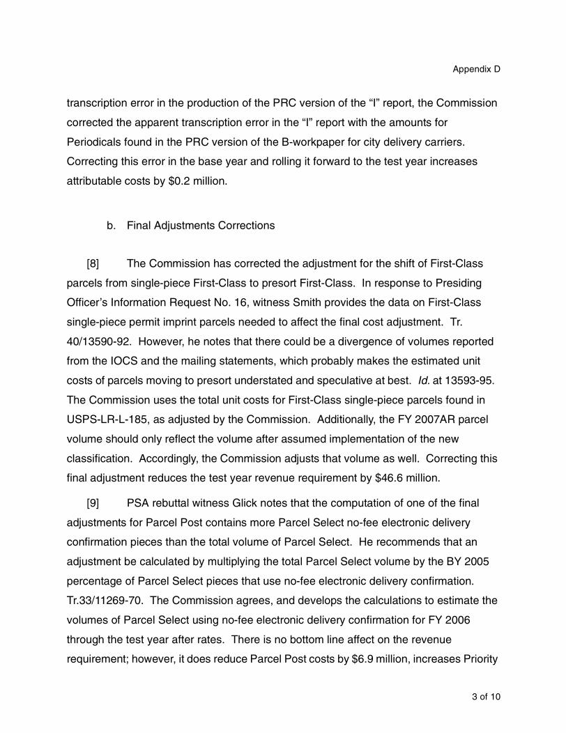
transcription error in the production of the PRC version of the “I” report, the Commission
corrected the apparent transcription error in the “I” report with the amounts for
Periodicals found in the PRC version of the B-workpaper for city delivery carriers.
Correcting this error in the base year and rolling it forward to the test year increases
attributable costs by $0.2 million.
b. Final Adjustments Corrections
[8] The Commission has corrected the adjustment for the shift of First-Class
parcels from single-piece First-Class to presort First-Class. In response to Presiding
Officer’s Information Request No. 16, witness Smith provides the data on First-Class
single-piece permit imprint parcels needed to affect the final cost adjustment. Tr.
40/13590-92. However, he notes that there could be a divergence of volumes reported
from the IOCS and the mailing statements, which probably makes the estimated unit
costs of parcels moving to presort understated and speculative at best. Id. at 13593-95.
The Commission uses the total unit costs for First-Class single-piece parcels found in
USPS-LR-L-185, as adjusted by the Commission. Additionally, the FY 2007AR parcel
volume should only reflect the volume after assumed implementation of the new
classification. Accordingly, the Commission adjusts that volume as well. Correcting this
final adjustment reduces the test year revenue requirement by $46.6 million.
[9] PSA rebuttal witness Glick notes that the computation of one of the final
adjustments for Parcel Post contains more Parcel Select no-fee electronic delivery
confirmation pieces than the total volume of Parcel Select. He recommends that an
adjustment be calculated by multiplying the total Parcel Select volume by the BY 2005
percentage of Parcel Select pieces that use no-fee electronic delivery confirmation.
Tr.33/11269-70. The Commission agrees, and develops the calculations to estimate the
volumes of Parcel Select using no-fee electronic delivery confirmation for FY 2006
through the test year after rates. There is no bottom line affect on the revenue
requirement; however, it does reduce Parcel Post costs by $6.9 million, increases Priority
3 of 10

Docket No. R2006-1
Mail costs by $3.3 million, and increases other special services costs by $3.6 million in
the test year after rates.
c. Summary
[10] Taking into account all of the revisions provided by the Postal Service and
the additional corrections made by the Commission, the revenue requirement for the test
year after rates, under PRC costing methodology, is reduced by $52.0 million.
B. Adjustments to Postal Service Compensation and Benefits Cost Factors for Known and Certain Events
[11] The Postal Service’s estimates for employee compensation and benefits are
influenced by: (1) assumptions regarding the results of labor negotiations or settlements;
(2) increases in the consumer price index; (3) management decisions regarding wage
changes for nonbargaining employees; and (4) changes in the cost structure of
employee benefits.
[12] In the Postal Service’s initial filing of May 3 , 2006, the FY 2006 estimates of
compensation and benefits for bargaining level employees were determined based on
the last year of labor contracts due to expire on November 20, 2006. The estimates for
FY 2007 and the test year were assumed to equal the Employment Cost Index less one
percent (ECI-1). Subsequent to the initial filing of this docket, two events occurred which
affected the original estimates of compensation and benefits. First, the COLA payment
for bargaining level employees due in September 2006 was substantially higher than
originally estimated by the Service. Tr. 19/6767-68. The Commission calculates the new
COLA payment and substitutes it for the original estimate. Second, the Office of
Personnel Management announced the average 2007 premium increase for the Federal
Health Benefits Program (FEHBP). The average increase of 1.8 percent was
substantially lower than the 7.0 percent estimated increase used by the Service. When
4 of 10
Appendix D
asked about the effect of the much lower FEHBP premium increase on Postal Service
costs, revenue requirement witness Loutsch noted that the real effect would not be
known until after the FEHBP open season, when employees can change plans.
However, he noted hat when the new premium rates were applied to the current
employee population, the increase was 2.3 percent. Id. at 6769-70. Consistent with past
practice, the Commission substitutes the 2.3 percent increase in health benefits for the
original estimate of 7 percent, but leaves the estimated increase for FY 2008 at the
original Postal Service estimate of 7 percent.
[13] PRC-LR-1 contains the workpapers filed by the Service in USPS-LR-L-50 as
adjusted for September 2006 COLA and the smaller increase in health benefits
premiums for FY 2007.
1. Adjustments Due to CPI-W Actual Results
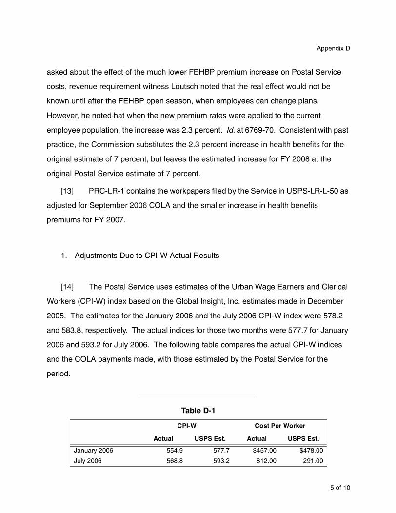
[14] The Postal Service uses estimates of the Urban Wage Earners and Clerical
Workers (CPI-W) index based on the Global Insight, Inc. estimates made in December
2005. The estimates for the January 2006 and the July 2006 CPI-W index were 578.2
and 583.8, respectively. The actual indices for those two months were 577.7 for January
2006 and 593.2 for July 2006. The following table compares the actual CPI-W indices
and the COLA payments made, with those estimated by the Postal Service for the
period.
Table D-1
CPI-W Cost Per Worker
Actual USPS Est. Actual USPS Est.
January 2006 554.9 577.7 $457.00 $478.00
July 2006 568.8 593.2 812.00 291.00
5 of 10

Docket No. R2006-1
[15] As the table above indicates, while the estimate for the January 2006 COLA
(payable in March 2006) is slightly lower than originally estimated, the estimate for the
July 2006 COLA (payable in September 2006) is significantly greater than originally
estimated. The effect of adjusting the COLA is to increase cost levels in the test year by
$429.3 million. Labor-related accrued costs for Repriced Annual Leave, Premium and
Benefit rollup costs, and the Workload Mix Adjustment also increase as a result of this
adjustment.
2. Adjustments Due to Actual Health Benefits Increases
[16] The Postal Service has estimated increases for FY 2007 and the test year in
the cost of providing health benefits to employees through the FEHBP. These increases
are based on a Hay Group analysis and are estimated to be 7 percent for both years. In
September 2006, the Office of Personnel Management announced that the average
premium increase for the FEHBP would be 1.8 percent for 2007. As noted above, the
Postal Service estimated that the increase, when applied to the current mix of employee
health plans, would yield a 2.3 percent increase for 2007. Accordingly, the Commission
applies this 2.3 percent estimated increase to health benefits costs, in lieu of the original
estimate of 7.0 percent. This smaller increase results in a reduction of cost levels of
$236.9 million.
[17] Additionally, the 2.3 percent health benefits increase is also applied to the
Annuitant Health Benefits model. This has the effect of reducing the costs of Annuitant
Health Benefits by $93 million.
3. Other Changes to Compensation and Benefits Cost Levels
[18] There are several other compensation-related costs that are effected by the
changes in COLA payments. The costs of premiums to basic pay, such as overtime and
6 of 10

Appendix D
night differential, and the costs of various compensation-related benefits such as Social
Security and CSRS/FERS retirement are directly tied to changes in the basic pay of
employees. Additionally, the costs of Repriced Annual Leave, Holiday Leave Variance,
and the workload mix adjustment are tied directly to changes in compensation. The net
effect is to increase costs by $149.7 million.
4. Adjustments to Cost Reductions and Other Programs
[19] The Postal Service has numerous programs and projects designed to
produce cost savings in the interim years and the test year. The Postal Service has
estimated these cost savings based on estimates of work hour savings by craft from the
implementation of the programs priced out at the estimated productive wage rate for the
particular craft. The effect of updating the cost level factors for the actual COLA and
health benefits will increase the savings estimates associated with these programs by
$9.5 million.
[20] Additionally, the cost reductions programs will have certain costs associated
with their implementation, and will increase the number of craft work hours. These costs
are included in Other Programs. The additional costs of other programs also are
estimated with the increased work hours by craft priced out at the estimated productive
wage rate for that particular craft. The effect of updating the cost levels for Actual
COLAs and health benefits increases these costs by $1.5 million.
5. Summary
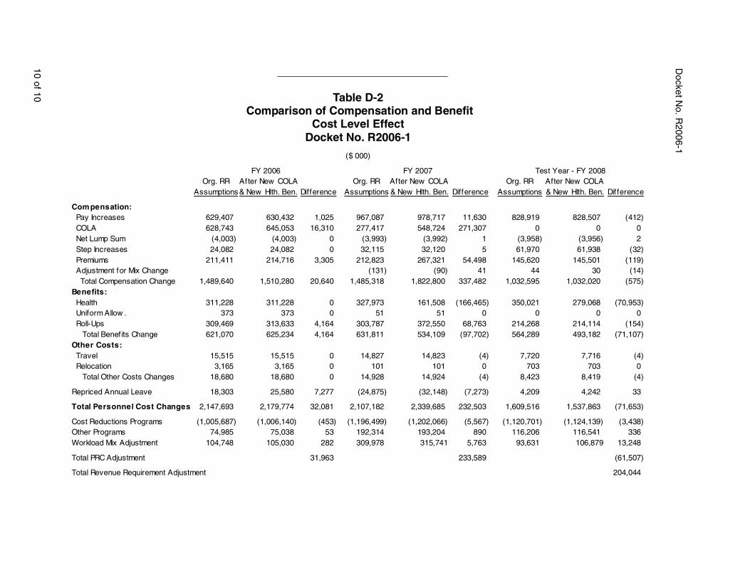
[21] The Commission adjustments to compensation and benefits cost estimates
through the test year increase the Postal Service’s estimated compensation and benefits
and other personnel-related test year expenses by approximately $204.0 million.
7 of 10

Docket No. R2006-1
Table D-2 summarizes the adjustments to compensation and benefits cost level, cost
reductions, and service-wide costs effects for FY 2006, FY 2007, and the test year.
C. Other Revenue Requirement Adjustments
[22] The Commission has lowered the estimate of base year registry mail
processing costs. This adjustment is based on re-allocating the mail processing costs of
registry using the RPW factor to split the Postal Service Penalty Registered mail costs
from the commercial registered mail costs. In Docket No. R2005-1, the Commission
rejected a Postal Service change in the allocation of these costs. The Commission again
rejects this change. See section V.F.12. This is applied in the B-workpaper for cost
segment 3, PRC LR-4, cs03 PRCfinal.xls, tab PRC 3.0.7 and tab 3.1.1. The results from
W/S 3.1.1a are transferred to the PRC version of the premium pay adjustment
calculations in USPS-LR-L-100. This adjustment increases the revenue requirement by
$19.1 million.
D. Implementation of the Commission’s Cost Attribution Methodologies and Revenue Requirement Changes
[23] For the purpose of developing the Commission’s test year attributable costs
and revenue requirement, changes were made to the Postal Service’s roll forward factor
files and the base year cost matrix. These changes are listed below:
• Adjustments to FY 2006, FY 2007, and the test year cost level factors, Cost Reductions Programs, Other Programs, and the work year mix adjustment, as discussed above;
• Attribution changes in cost segments 3 and 14, as discussed in the Opinion;
• Adjustments of volumes and revenues for corrections to the volume and revenue estimation models and also for PRC adjustments to rates.
8 of 10

Appendix D
[24] The adjustments made to Postal Service costs are calculated using the PRC
version of the revenue requirement workpapers, PRC-LR-1 and the Commission’s
CRA/Cost roll forward model, PRC-LR-2.
9 of 10
10 of 10
Docket N
o. R2006-1
Test Year - FY 2008 RR After New COLAptions & New Hlth. Ben. Dif ference
8,919 828,507 (412)0 0 0
3,958) (3,956) 21,970 61,938 (32)5,620 145,501 (119)
44 30 (14)2,595 1,032,020 (575)
0,021 279,068 (70,953)0 0 0
4,268 214,114 (154)4,289 493,182 (71,107)
7,720 7,716 (4)703 703 0
8,423 8,419 (4)
4,209 4,242 33
9,516 1,537,863 (71,653)
0,701) (1,124,139) (3,438)6,206 116,541 3363,631 106,879 13,248
(61,507)
204,044
Table D-2 Comparison of Compensation and Benefit
Cost Level EffectDocket No. R2006-1
FY 2006 FY 2007Org. RR After New COLA Org. RR After New COLA Org.
Assumptions & New Hlth. Ben. Difference Assumptions & New Hlth. Ben. Difference Assum
Compensation: Pay Increases 629,407 630,432 1,025 967,087 978,717 11,630 82 COLA 628,743 645,053 16,310 277,417 548,724 271,307 Net Lump Sum (4,003) (4,003) 0 (3,993) (3,992) 1 ( Step Increases 24,082 24,082 0 32,115 32,120 5 6 Premiums 211,411 214,716 3,305 212,823 267,321 54,498 14 Adjustment for Mix Change (131) (90) 41 Total Compensation Change 1,489,640 1,510,280 20,640 1,485,318 1,822,800 337,482 1,03Benefits: Health 311,228 311,228 0 327,973 161,508 (166,465) 35 Uniform Allow . 373 373 0 51 51 0 Roll-Ups 309,469 313,633 4,164 303,787 372,550 68,763 21 Total Benef its Change 621,070 625,234 4,164 631,811 534,109 (97,702) 56Other Costs: Travel 15,515 15,515 0 14,827 14,823 (4) Relocation 3,165 3,165 0 101 101 0 Total Other Costs Changes 18,680 18,680 0 14,928 14,924 (4)
Repriced Annual Leave 18,303 25,580 7,277 (24,875) (32,148) (7,273)
Total Personnel Cost Changes 2,147,693 2,179,774 32,081 2,107,182 2,339,685 232,503 1,60
Cost Reductions Programs (1,005,687) (1,006,140) (453) (1,196,499) (1,202,066) (5,567) (1,12Other Programs 74,985 75,038 53 192,314 193,204 890 11Workload Mix Adjustment 104,748 105,030 282 309,978 315,741 5,763 9
Total PRC Adjustment 31,963 233,589
Total Revenue Requirement Adjustment
($ 000)

Appendix ECOMPARISON OF COSTS ATTRIBUTED BY COST SEGMENT AND COMPONENT
PRC R2006-1 Test Year USPS R2006-1 Test YearAccrued Attributable Percent Accrued Attributable Percent
Cost Cost Attributable Cost Cost Attributable
1. Postmasters EAS 22 and Below 2,397,817 423,768 17.67 2,406,927 424,556 17.64 EAS 23 and Above 60,845 - 0.00 61,102 - 0.00 Total 2,458,662 423,768 17.24 2,468,028 424,556 17.20
2. Supervisors & Technical Personnel Mail Processing 1,001,203 942,114 94.10 1,006,123 841,389 83.63 Window Service 267,379 98,150 36.71 267,793 99,225 37.05 Time and Attendance 73,432 44,565 60.69 73,637 41,994 57.03 Employee & Labor Relations - - 0.00 - - 0.00 City Carriers 1,154,253 584,847 50.67 1,155,719 584,300 50.56 Rural Carriers 116,415 47,572 40.86 116,608 47,522 40.75 Vehicle Service 41,851 25,072 59.91 41,871 25,033 59.79 Higher Level Supervisors 269,373 77,611 28.81 269,824 72,959 27.04 Superv. Qual. Cntrl./Rev. Prot. 50,802 46,987 92.49 50,993 42,867 84.06 Superv. Central Mail Mark-Up 46,400 46,372 99.94 46,916 39,613 84.43 Joint Supv. Clerks & Carriers 619,165 424,682 68.59 620,872 398,173 64.13 Gen.Supv., Mail Process. - - 0.00 - - 0.00 Gen.Supv., Coll.& Del. - - 0.00 - - 0.00 Other Sup., Training 49,258 27,274 55.37 49,405 25,576 51.77 Other 716,653 - 0.00 719,207 - 0.00 Total 4,406,184 2,365,246 53.68 4,418,969 2,218,650 50.21
3. Clerks & Mailhandlers, CAG A-J Mail Processing 14,243,015 13,380,667 93.95 14,586,630 12,107,043 83.00 Window Service 2,825,660 1,037,244 36.71 2,724,101 985,231 36.17 Administrative Clerks 1,485,308 968,383 65.20 1,109,123 675,325 60.89 Time & Attendance 72,434 43,959 60.69 62,829 35,830 57.03 Specific Fixed 10,315 10,315 100.00 10,253 - 0.00 Total 18,636,732 15,440,569 82.85 18,492,936 13,803,429 74.64
4. Clerks, CAG K 6,733 3,673 54.55 6,673 3,631 54.41
6. City Carrier In-Office Direct Labor 3,890,140 3,339,298 85.84 3,857,993 3,317,946 86.00 Support Overhead 912,866 786,266 86.13 905,404 779,349 86.08 Support Other 567,268 288,410 50.84 563,547 285,890 50.73 Total 5,370,274 4,413,974 82.19 5,326,944 4,383,185 82.28
7. City Carrier Street Delivery Activities 8,817,713 3,682,779 41.77 8,763,592 3,650,789 41.66 Delivery Activities Support 1,120,366 484,129 43.21 1,113,405 479,910 43.10 Network Travel 1,484,523 - 0.00 1,478,125 - 0.00 Network Travel Support 225,557 - 0.00 224,585 - 0.00 Total 11,648,158 4,166,908 35.77 11,579,708 4,130,699 35.67
Grand Total City Carriers 17,018,433 8,580,882 50.42 16,906,652 8,513,885 50.36
($ 000's)
1 of 3

Docket No. R2006-1
PRC R2006-1 Test Year USPS R2006-1 Test YearAccrued Attributable Percent Accrued Attributable Percent
Cost Cost Attributable Cost Cost Attributable
Comparison of Costs Attributed byCost Segment and Component
($ 000's)
8. Vehic le Service Drivers 670,560 401,724 59.91 665,227 397,706 59.79
10. Rural Carriers Evaluated Routes 5,494,112 2,246,904 40.90 5,451,709 2,224,911 40.81 Other Routes 503,544 197,080 39.14 499,719 195,178 39.06 Equip. Maint. A llow. 494,236 - 0.00 494,236 - 0.00 Total 6,491,892 2,443,984 37.65 6,445,665 2,420,088 37.55
11. Custodial Maint. Service Custodial Personnel 1,190,300 725,080 60.92 1,183,684 709,278 59.92 Operating Equipment Maint 1,628,910 1,354,686 83.17 1,631,467 1,143,347 70.08 B ldg. & Plant Maint. Person 595,909 363,002 60.92 594,015 355,941 59.92 Contract Cleaners 100,623 61,295 60.92 100,623 60,295 59.92 Total 3,515,742 2,504,064 71.22 3,509,789 2,268,861 64.64
12. Motor Vehic le Service Personnel 475,730 114,399 24.05 473,229 113,397 23.96 Supplies & Materials 657,467 170,685 25.96 656,665 169,884 25.87 Vehic le Hire 14,301 6,888 48.16 14,270 6,857 48.05 Total 1,147,498 291,971 25.44 1,144,163 290,137 25.36
13. M isc. Operating Costs Drive out and Carfare 34,956 4,413 12.62 34,936 4,393 12.57 Tolls & Ferriage 551 - 0.00 551 - 0.00 Other 333,895 - 0.00 334,077 - 0.00 Total 369,402 4,413 1.19 369,564 4,393 1.19
14. Transportation Domestic Air 1,439,853 1,439,550 99.98 1,456,743 1,260,702 86.54 A laskan Air 116,752 8,196 7.02 115,115 8,081 7.02 Highway 3,004,555 2,381,589 79.27 2,995,138 2,372,185 79.20 Railroad 131,001 129,611 98.94 130,219 128,829 98.93 Domestic W ater 30,059 26,260 87.36 29,900 26,102 87.30 International W ater 699,808 699,812 100.00 699,771 699,775 100.00 Total 5,422,028 4,685,018 86.41 5,426,886 4,495,674 82.84
15. Building Occupancy Rents 970,662 970,662 100.00 970,662 970,662 100.00 Fuel & Utilit ies 649,337 395,549 60.92 649,337 389,091 59.92 Other 375,593 716 0.19 375,593 - 0.00 Total 1,995,593 1,366,927 68.50 1,995,593 1,359,753 68.14
2 of 3

PRC R2006-1 Test Year USPS R2006-1 Test YearAccrued Attributable Percent Accrued Attributable Percent
Cost Cost Attributable Cost Cost Attributable
Comparison of Costs Attributed byCost Segment and Component
($ 000's)
16. Supplies & Services Custodial & Building 174,601 106,359 60.92 174,601 104,623 59.92 Operating Equip. Maintenan 536,646 345,890 64.45 540,930 285,420 52.76 Stamps & Dispensers 87,478 87,175 99.65 86,623 86,321 99.65 Advertising 127,834 65,377 51.14 127,834 - 0.00 Stmp. Cds. & Emb. Stmp. 8,667 8,667 100.00 8,643 8,643 100.00 Money Orders 5,594 5,594 100.00 5,512 5,512 100.00 Misc. Attrib. PMPC/Intl/DC 86,330 86,330 100.00 86,330 86,330 100.00 Misc. Postal Supp. & Serv. 1,105,837 659,223 59.61 1,105,009 618,021 55.93 Other 697,252 16,136 2.31 697,221 401 0.06 Total 2,830,238 1,380,752 48.79 2,832,701 1,195,270 42.20
18. Administrative & Regional Operations Workers Compensation 1,236,630 505,940 40.91 1,236,630 475,123 38.42 Repriced Annual Leave 82,650 48,594 58.79 82,613 45,614 55.21 Holiday Leave 924 543 58.79 924 510 55.21 Retiree Health Benefits 2,026,057 1,191,216 58.79 2,119,140 1,170,052 55.21 Annuitant Life Insurance 15,200 8,937 58.79 15,200 8,392 55.21 USPS Protection Force 78,505 47,822 60.92 78,234 46,879 59.92 Unemployment Compensati 64,373 37,848 58.79 64,373 35,543 55.21 CSRS Reform Escrow 3,588,223 - 0.00 3,588,223 - 0.00 CSRS/FERS Retire. Prin. 32,590 - 0.00 32,590 - 0.00 Money Orders 86 86 100.00 86 86 100.00 Other Personnel 1,638,362 12,510 0.76 1,641,272 - 0.00 Other 287,367 24,296 8.45 287,367 - 0.00 Total 9,050,967 1,877,793 20.75 9,146,653 1,782,199 19.48
20. Depreciation & Other Servicewide Costs Vehicle Deprec. 234,300 56,453 24.09 234,300 56,324 24.04 Mail Proc. Equip. Deprec. 1,513,106 819,422 54.15 1,513,106 729,448 48.21 Bldg. & Leasehold Deprec. 774,667 774,667 100.00 774,667 774,667 100.00 Indemnities 127,112 26,076 20.51 126,954 25,919 20.42 Note Interest Expense 84,021 54,987 65.44 84,019 51,984 61.87 Retirement Interest Expens 257,410 - 0.00 257,410 - 0.00 Other Interest 84,961 - 0.00 84,961 - 0.00 Other (10,628) - 0.00 (10,628) - 0.00 Total 3,064,949 1,731,604 56.50 3,064,789 1,638,342 53.46
17. Res., Develop., & Engr. 42,001 - 0.00 42,001 - 0.0019. Support Services 68,318 145 0.21 68,331 - 0.00
Final Adjustments (407,160) (976,711) (243,166) (711,781)
Grand Total All Segments 76,788,770 42,525,822 55.38 76,761,455 40,104,793 52.25
3 of 3


1 of 4
Contingency Grand Total
PRC Distribution of Attributable Costs to Classes and SubclassesTest Year/PRC Recommended Rates
($000)Short ProductRun Specific PESSA Total Final Net
App
endix FP
RC
DIS
TR
IBU
TIO
N O
F
AT
TR
IBU
TA
BLE
CO
ST
S T
O C
LAS
SE
S A
ND
SU
BC
LAS
SE
S
@ 1.0 percent Attributable
111,975 11,309,44155,192 5,574,400
167,167 16,883,8415,902 596,0582,624 264,9808,525 861,038
175,692 17,744,87934,318 3,466,1084,626 467,208
(0) (0)
810 81,77823,650 2,388,69624,460 2,470,474
28,409 2,869,295101,319 10,233,250129,728 13,102,545
12,662 1,278,8406,543 660,8284,024 406,429
23,229 2,346,0970 0
720 72,753392,773 39,670,06414,902 1,505,112
407,675 41,175,177
357 36,091791 79,910
4,659 470,51274 7,484
1,479 149,42817 1,681
130 13,12410 1,040
6,029 608,9764,036 407,658
17,583 1,775,904 425,258 42,951,081342,629 34,605,577767,888 77,556,658
9,374 77,566,032
Variable Costs Costs Attributable Adjustments AttributableFirst-Class Mail: Single-Piece Letters 9,902,026 6,191 1,455,286 11,363,503 (166,036) 11,197,467 Presort Letters 4,743,360 7,003 624,340 5,374,703 144,505 5,519,208 Total Letters 14,645,386 13,194 2,079,625 16,738,205 (21,531) 16,716,674 Single-Piece Cards 522,858 359 66,940 590,157 0 590,157 Presort Postcards 236,054 443 31,330 267,828 (5,471) 262,356 Total Cards 758,911 803 98,270 857,985 (5,471) 852,513 Total First-Class 15,404,297 13,997 2,177,896 17,596,190 (27,003) 17,569,187Priority Mail 3,078,366 49,793 308,619 3,436,778 (4,988) 3,431,790Express Mail 401,347 12,330 48,904 462,582 0 462,582Mailgrams (0) - (0) (0) 0 (0)Periodicals: Within County 72,174 6 8,789 80,968 0 80,968 Outside County 2,055,008 65 309,971 2,365,045 0 2,365,045 Total Periodicals 2,127,182 72 318,760 2,446,014 0 2,446,014Standard Mail: Enhanced Carrier Route 2,702,570 4,946 314,053 3,021,569 (180,683) 2,840,886 Regular Bulk & Nonprofit 8,988,697 9,310 1,332,554 10,330,561 (198,630) 10,131,931 Total Standard Mail 11,691,267 14,256 1,646,607 13,352,129 (379,312) 12,972,817Package Services: Parcel Post 1,068,622 74 128,587 1,197,283 68,895 1,266,179 Bound Printed Matter 569,183 - 85,102 654,285 0 654,285 Media and Library 352,751 - 49,654 402,405 0 402,405 Total Package Services 1,990,557 74 263,342 2,253,973 68,895 2,322,869USPS Penalty Mail 492,980 - 76,570 569,551 (569,551) 0Free Mail for the Blind & Hndc 61,269 - 10,763 72,033 0 72,033 TOTAL DOMESTIC MAIL 35,247,267 90,522 4,851,461 40,189,250 (911,958) 39,277,291International Mail 1,365,182 32,324 92,704 1,490,210 0 1,490,210 TOTAL ALL MAIL 36,612,449 122,846 4,944,165 41,679,460 (911,958) 40,767,501 Special Services: Registered Mail 27,056 - 8,678 35,734 0 35,734 Insured Mail 88,548 252 9,423 98,224 (19,105) 79,119 Certif ied Mail 418,786 33 47,034 465,853 0 465,853 Collect-on-Delivery 6,820 - 589 7,410 0 7,410 Money Orders 125,005 3,607 19,337 147,949 0 147,949 Stamped Cards 1,662 - 2 1,664 0 1,664 Stamped Envelopes 12,162 - 832 12,994 0 12,994 Special Handling 877 - 153 1,030 0 1,030 Post Off ice Boxes 52,895 1,103 548,949 602,947 0 602,947 Other Special Services 395,291 1,985 51,993 449,269 (45,647) 403,622Total Special Services 1,129,103 6,980 686,991 1,823,073 (64,752) 1,758,321 Total Attributable 37,741,552 129,825 5,631,156 43,502,533 (976,711) 42,525,823 Other Costs 39,454,378 (129,825) (5,631,156) 33,693,397 569,551 34,262,948 Total Costs 77,195,930 77,195,930 (407,160) 76,788,770Prior Years Loss RecoveryTotal Revenue Requirement

2 of 4
Docket N
o. R2006-1
Motor Misc.Vehicle OperatingService Costs
53,283 1,173 34,755 683 88,038 1,855 3,469 87 1,991 39 5,460 126
93,498 1,982 24,939 81 2,433 15
- -
1,103 12 14,510 267 15,613 280
38,094 532 65,755 1,261
103,849 1,793
21,369 38 13,626 43 3,749 15
38,744 96 1,225 51
330 4 280,631 4,302
3,333 17 283,964 4,319
113 1 4,751 56
492 4 65 0 25 -
- - - - - - - -
2,563 32 8,007 94
291,971 4,413 855,527 364,990
1,147,498 369,402
($000)
PRC Distribution of Attributable Costs to Classes and SubclassesTest Year/PRC Recommended Rates
Clerks & City Vehicle CustodialPost- Mailhandlers Clerks, Delivery Service Rural Maintenance
Masters Supervisors CAG A - J CAG K Carriers Drivers Carriers ServiceFirst-Class Mail: Single-Piece Letters 109,351 690,310 4,850,645 1,361 2,279,509 21,798 299,389 788,579 Presort Letters 92,927 309,826 1,811,768 523 1,324,796 26,188 319,835 297,810 Total Letters 202,278 1,000,136 6,662,413 1,884 3,604,305 47,986 619,225 1,086,389 Single-Piece Cards 3,643 38,216 232,295 61 168,613 230 21,643 31,800 Presort Post Cards 3,970 16,118 84,973 25 77,715 536 21,107 13,613 Total Cards 7,613 54,334 317,269 86 246,327 765 42,750 45,413 Total First-Class 209,890 1,054,470 6,979,681 1,970 3,850,633 48,751 661,975 1,131,802Priority Mail 27,778 125,573 1,089,954 313 186,509 74,102 47,961 113,915 Express Mail 4,304 24,001 229,371 - 34,926 1,364 10,528 13,251 Mailgrams - (0) (0) - - - - (0) Periodicals: Within County 428 4,788 23,222 - 24,068 2,016 13,024 2,319 Outside County 12,850 147,090 845,488 - 467,396 31,505 148,503 123,810 Total Periodicals 13,278 151,878 868,710 - 491,464 33,521 161,527 126,129 Standard Mail: Enhanced Carrier Route 35,275 159,918 573,697 105 1,040,344 46,637 562,983 97,334 Regular Bulk & Nonprofit 95,141 591,356 3,739,142 747 2,415,058 63,064 724,433 627,811 Total Standard Mail 130,416 751,273 4,312,839 853 3,455,402 109,702 1,287,416 725,144 Package Services: Parcel Post 7,498 48,242 366,322 71 92,951 78,122 37,146 51,499 Bound Printed Matter 4,287 32,256 209,640 44 105,630 34,782 31,512 39,535 Media and Library 2,032 16,769 137,929 27 36,144 9,114 11,448 25,011 Total Package Services 13,816 97,267 713,891 142 234,725 122,018 80,106 116,045 USPS Penalty Mail - 38,882 299,797 - 78,352 3,812 3,160 27,498 Free Mail for the Blind & Hndc - 3,802 31,311 - 7,009 773 2,901 5,393 TOTAL DOMESTIC MAIL 399,483 2,247,147 14,525,553 3,278 8,339,020 394,044 2,255,574 2,259,176International Mail 8,771 37,925 356,881 1 36,675 7,680 20,121 40,821 TOTAL ALL MAIL 408,254 2,285,072 14,882,433 3,278 8,375,696 401,724 2,275,695 2,299,997Special Services: Registered Mail 253 1,939 17,767 69 2,278 - 1,609 2,708 Certif ied Mail 3,872 26,660 134,804 101 120,817 - 110,611 9,514 Insured Mail 653 5,431 38,227 5 9,564 - 14,518 1,964 Collect-On-Delivery 47 319 1,981 2 974 - 1,595 120 Money Orders 1,241 11,365 99,407 - - - 1,242 4,288 Stamped Cards 14 0 0 - - - - 1 Stamped Envelopes 134 486 4,260 - - - - 187 Special Handling 61 66 692 1 - - - 44 Post Off ice Boxes 5,183 4,846 40,685 - - - - 165,903 Other Special Services 4,055 29,062 220,313 217 71,554 - 38,714 19,338 Total Special Services 15,513 80,174 558,137 395 205,186 - 168,289 204,066 Total Attributable 423,768 2,365,246 15,440,570 3,673 8,580,882 401,724 2,443,984 2,504,064Other Costs 2,034,894 2,040,938 3,196,161 3,060 8,437,551 268,836 4,047,908 1,011,678Total Costs 2,458,662 4,406,184 18,636,732 6,733 17,018,433 670,560 6,491,892 3,515,742Prior Years Loss RecoveryTotal Revenue Requirement

3 of 4
Appe
ndix F
Total PRCnal Attributabletments Contingency Costs
66,036) 111,975 11,309,44144,505 55,192 5,574,400 21,531) 167,167 16,883,841
- 5,902 596,058 (5,471) 2,624 264,980 (5,471) 8,525 861,038 27,003) 175,692 17,744,879(4,988) 34,318 3,466,108
- 4,626 467,208 - (0) (0)
- 810 81,778 - 23,650 2,388,696 - 24,460 2,470,474
80,683) 28,409 2,869,295 98,630) 101,319 10,233,25079,312) 129,728 13,102,545
68,895 12,662 1,278,840 - 6,543 660,828 - 4,024 406,429
68,895 23,229 2,346,097 69,551) - -
- 720 72,753 11,958) 392,773 39,670,064
- 14,902 1,505,112 11,958) 407,675 41,175,177
- 357 36,091 - 4,659 470,512
19,105) 791 79,910 - 74 7,484 - 1,479 149,428 - 17 1,681 - 130 13,124 - 10 1,040 - 6,029 608,976
45,647) 4,036 407,658 64,752) 17,583 1,775,904 76,711) 425,258 42,951,08169,551 342,629 34,605,57707,160) 767,888 77,556,658
9,374 77,566,032
PRC Distribution of Attributable Costs to Classes and SubclassesTest Year/PRC Recommended Rates
($000)
Admin. & General Depreciation TotalTrans- Building Supplies & Research & Regional Management & Service- Attributable Fiportation Occupancy Services Development Operations Systems w ide Costs Costs Adjus
First-Class Mail: 532,637 324,947 424,816 - 520,998 - 464,708 11,363,503 (1 Single-Piece Letters 438,321 132,570 137,937 - 244,769 - 201,995 5,374,703 1 Presort Letters 970,957 457,517 562,753 - 765,767 - 666,703 16,738,205 ( Total Letters 6,118 14,540 21,709 - 28,524 - 19,209 590,157 Single-Piece Cards 11,454 6,677 7,003 - 12,833 - 9,774 267,828 Presort Postcards 17,572 21,217 28,712 - 41,357 - 28,983 857,985 Total Cards 988,529 478,734 591,464 - 807,124 - 695,686 17,596,190 (
1,303,573 81,716 173,499 - 105,287 - 81,576 3,436,778 Priority Mail 75,209 13,624 25,000 - 18,181 - 10,378 462,582 Express Mail - (0) (0) - (0) - (0) (0)
Periodicals: 94 2,049 1,829 - 3,976 - 2,039 80,968 Within County 240,001 70,741 60,604 - 101,511 - 100,769 2,365,045 Outside County 240,095 72,790 62,433 - 105,486 - 102,808 2,446,014
Standard Mail: 106,171 72,409 71,132 - 143,126 - 73,813 3,021,569 (1 Enhanced Carrier Route 520,624 293,330 289,472 - 470,415 - 432,951 10,330,561 (1 Regular Bulk & Nonprofit 626,795 365,739 360,604 - 613,541 - 506,764 13,352,129 (3
Package Services: 361,181 31,375 22,291 - 39,389 - 39,787 1,197,283 Parcel Post 93,602 19,622 14,908 - 26,395 - 28,403 654,285 Bound Printed Matter 109,141 11,890 8,574 - 13,743 - 16,820 402,405 Media and Library 563,924 62,888 45,773 - 79,528 - 85,011 2,253,973
32,651 16,413 15,264 - 25,680 - 26,765 569,551 (5 USPS Penalty Mail 9,536 2,646 1,883 - 2,945 - 3,501 72,033
3,840,312 1,094,550 1,275,921 - 1,757,772 - 1,512,488 40,189,250 (9 TOTAL DOMESTIC MAIL 844,706 23,610 36,214 - 39,628 145 33,681 1,490,210 International Mail 4,685,018 1,118,160 1,312,134 - 1,797,400 145 1,546,170 41,679,460 (9 Special Services: Registered Mail - 2,885 953 - 1,582 - 3,577 35,734 Certif ied Mail - 11,558 10,855 - 23,061 - 9,193 465,853 Insured Mail - 2,456 2,508 - 4,000 - 18,402 98,224 ( Collect-On-Delivery - 146 138 - 286 - 1,737 7,410 Money Orders - 5,398 10,151 - 10,503 - 4,329 147,949 Stamped Cards - 1 1,647 - 1 - 0 1,664 Stamped Envelopes - 235 7,217 - 289 - 187 12,994 Special Handling - 38 32 - 49 - 45 1,030 Post Off ice Boxes - 212,868 18,232 - 18,828 - 136,402 602,947 Other Special Services - 13,182 16,885 - 21,793 - 11,562 449,269 ( Total Special Services - 248,768 68,618 - 80,393 - 185,435 1,823,073 ( Total Attributable 4,685,018 1,366,927 1,380,752 - 1,877,793 145 1,731,604 43,502,533 (9 Other Costs 737,010 628,666 1,449,486 42,001 7,173,174 68,172 1,333,344 33,693,397 5 Total Costs 5,422,028 1,995,593 2,830,238 42,001 9,050,967 68,318 3,064,949 77,195,930 (4 Prior Years Loss RecoveryTotal Revenue Requirement

Docket No. R2006-1
Unit Attributable Cost ComparisonTest Year
PRC PRC Change OverR2005-1 R2006-1 PRC R2005-1
($) ($) (%)First-Class Single Letter 0.2840 0.3019 6.30% Presort Letter 0.1030 0.1165 13.19% Total Letter 0.1882 0.1979 5.19%
Cards 0.1448 0.1501 3.62%
Priority Mail 3.9073 4.1808 7.00%
Express Mail 9.6074 10.9460 13.93%
Periodicals: Within County 0.0932 0.1160 24.45% Outside County 0.2607 0.2969 13.89%
Standard Mail: Enhanced Carrier Route 0.0723 0.0891 23.21% Regular Bulk & Nonprofit 0.1390 0.1348 -3.01% Total Standard Mail 0.1160 0.1212 4.47%
Package Services: Parcel Post 3.1653 3.4096 7.72% Bound Printed Matter 0.9128 1.0090 10.54% Media and Library 2.1043 2.4480 16.33%
Free for the Blind 0.6243 0.8313 33.17%International Mail 1.7817 1.9509 9.50%
Registry 10.5605 10.2832 -2.62%Certified 1.6616 1.7922 7.86%Insurance 1.9751 1.9134 -3.13%COD 4.8509 6.3788 31.50%Money Orders 0.7473 0.9693 29.72%
4 of 4

1 of 51
ost Change in rage Rev./Pc.
11.6% 7.0%
Test Year (2008) Volume, Cost, Revenue, and Cost Coverage by ClassALL_R06.XLS at Commission Recommended Rates
01:35 PM Contribution to Contribution toAttributable Institutional Institutional
Volume Revenue Cost Cost Rev./Pc. Cost/Pc. Cost/Pc. C(000) ($ 000) ($ 000) ($ 000) (Cents) (Cents) (Cents) Cove
First-Class MailLetters 85,295,205 35,732,311 16,883,841 18,848,470 41.893 19.795 22.098 2
App
endix G
Sche
dule 1
TE
ST
YE
AR
VO
LUM
E, C
OS
T, R
EV
EN
UE
, A
ND
CO
ST
CO
VE
RA
GE
BY
CLA
SS
55.4% 6.1%49.8% 13.6%70.4% 12.5%
00.1% 18.3%00.2% 11.7%
9.5%6.7%
70.8% 9.3%6.9%8.8%
06.3% 6.9%
13.9% 16.6%19.4% 11.7%
17.9%17.4%
03.7% 17.8%
24.9% 8.8%78.4% 7.6%
32.1% 20.7%29.5% -5.6%47.9% 10.4%10.3% 7.9%50.0% 8.8%35.2% 0.0%56.6% 10.1%04.1% 10.6%
79.3% 7.6%
Cards 5,738,035 1,338,036 861,038 476,997 23.319 15.006 8.313 1Priority Mail 829,047 5,192,582 3,466,108 1,726,474 626.331 418.083 208.248 1Express Mail 42,683 796,283 467,208 329,075 1,865.572 1,094.599 770.974 1Periodicals
Within County 731,966 81,832 81,778 54 11.180 11.172 0.007 1Outside County 8,045,116 2,392,300 2,388,696 3,604 29.736 29.691 0.045 1
Standard MailRegular 63,478,847 15,672,195 24.689Nonprofit 12,416,064 1,802,679 14.519
Regular and Nonprofit 75,894,910 17,474,874 10,233,250 7,241,624 23.025 13.483 9.542 1Enhanced Carrier Route (ECR) 29,677,241 5,624,459 18.952Nonprofit ECR (NECR) 2,529,325 293,963 11.622
ECR and NECR 32,206,566 5,918,422 2,869,295 3,049,127 18.376 8.909 9.467 2Package Services
Parcel Post 375,070 1,456,748 1,278,840 177,907 388.394 340.960 47.433 1Bound Printed Matter 654,923 788,965 660,828 128,138 120.467 100.902 19.565 1
Media Mail 153,674 390,476 254.093Library Rate 12,352 30,829 249.583
Media and Library 166,026 421,305 406,429 14,875 253.758 244.798 8.960 1USPS Penalty Mail 646,024Free-for-the-Blind Mail 87,514 72,753 (72,753) 83.133International Mail 1/ 771,496 1,880,630 1,505,112 375,518 243.764 195.090 48.674 1
Total All Mail 211,484,583 73,474,287 41,175,177 32,299,110 34.742 19.470 15.273 1Special Services
Registry 3,510 47,660 36,091 11,568 1,357.927 1,028.324 329.602 1Insurance 41,764 103,509 79,910 23,599 247.842 191.337 56.505 1Certif ied 262,526 695,695 470,512 225,183 265.000 179.224 85.776 1COD 1,173 8,258 7,484 774 703.868 637.877 65.991 1Money Orders 154,155 224,143 149,428 74,715 145.401 96.933 48.467 1Stamped Cards 113,618 2,272 1,681 592 2.000 1.479 0.521 1Box/Caller Service 16,343 953,886 608,976 344,909 5,836.794 3,726.305 2,110.489 1Stamped Envelopes 300,000 13,657 13,124 533 4.552 4.375 0.178 1Other Special Services 752,818 408,698 344,119
Other Income 755,735 755,735Total Mail & Services 211,484,583 77,031,918 42,951,081 34,080,837 36.424 20.309 16.115 1
Institutional Costs 34,605,577Prior Years Loss Recovery 9,374Appropriations 101,593Investment Income 434,831
Total Revenues 77,568,342Total Revenue Requirement 77,566,032
Net Surplus (Loss) 2,3101/ Not subject to PRC jurisdiction.

Docket No. R2006-1
FIRST-CLASS MAIL Units Rate Revenues(000) (cents) (000)
Letters & Sealed Parcels Subclass
RegularSingle-Piece
Letters, First Oz., except QBRM 33,772,329 41.0 13,846,655 Flats, First Oz. 3,097,650 80.0 2,478,120 Parcels, First Oz. 270,143 113.0 305,262 Additional ounces 11,731,577 17.0 1,994,368 Nonmachinable Letters < 1oz. 113,765 17.0 19,340 Qualified Business Reply Mail 321,668 38.0 122,234
Total Pieces (or Postage Revenue) 37,461,791 18,765,979 Revenue x Adjustment Factor 19,035,616
Single-Piece Fees Address Correction 14,345 Business Reply 184,262 Certificate of Mailing 2,093 Merchandise Return 117 Shipper Paid Forwarding 1 Special Handling 10,362
Total Single-Piece Revenue 19,246,795
PresortLetters, First Oz. 1,048,381 37.3 391,046 Flats, First Oz. 106,308 69.9 74,309 Additional ounces 264,118 17.0 44,900 Nonmachinable Letters < 1oz. 14,342 17.0 2,438
Total Pieces (or Postage Revenue) 1,154,688 512,693 Revenue x Adjustment Factor 515,450
Presort Fees Address Correction 442 Certificate of Mailing 7 Merchandise Return 4 Presort Permit 153 Shipper Paid Forwarding 0
Total Presort Revenue 516,055
Total Regular Letters 38,616,479 19,762,851
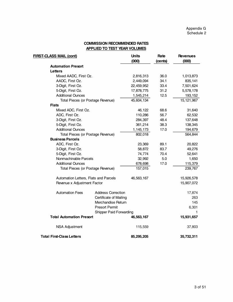
COMMISSION RECOMMENDED RATESAPPLIED TO TEST YEAR VOLUMES
2 of 51
Appendix GSchedule 2
Automation PresortLetters
Mixed AADC, First Oz. 2,816,313 36.0 1,013,873 AADC, First Oz. 2,449,094 34.1 835,141 3-Digit, First Oz. 22,459,952 33.4 7,501,624 5-Digit, First Oz. 17,878,775 31.2 5,578,178 Additional Ounces 1,545,214 12.5 193,152
Total Pieces (or Postage Revenue) 45,604,134 15,121,967 Flats
Mixed ADC, First Oz. 46,122 68.6 31,640 ADC, First Oz. 110,286 56.7 62,532 3-Digit, First Oz. 284,397 48.4 137,648 5-Digit, First Oz. 361,214 38.3 138,345 Additional Ounces 1,145,173 17.0 194,679
Total Pieces (or Postage Revenue) 802,018 564,844 Business Parcels
ADC, First Oz. 23,369 89.1 20,822 3-Digit, First Oz. 58,872 83.7 49,276 5-Digit, First Oz. 74,774 70.4 52,641 Nonmachinable Parcels 32,992 5.0 1,650 Additional Ounces 678,698 17.0 115,379
Total Pieces (or Postage Revenue) 157,015 239,767
Automation Letters, Flats and Parcels 46,563,167 15,926,578 Revenue x Adjustment Factor 15,907,072
Automation Fees Address Correction 17,874 Certificate of Mailing 263 Merchandise Return 145 Presort Permit 6,301 Shipper Paid Forwarding 1
Total Automation Presort 46,563,167 15,931,657
NSA Adjustment 115,559 37,803
Total First-Class Letters 85,295,205 35,732,311
FIRST-CLASS MAIL (cont) Units Rate Revenues(000) (cents) (000)
COMMISSION RECOMMENDED RATESAPPLIED TO TEST YEAR VOLUMES
3 of 51
Docket No. R2006-1
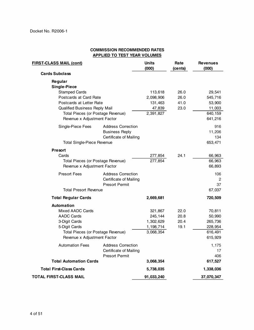
FIRST-CLASS MAIL (cont) Units Rate Revenues(000) (cents) (000)
Cards Subclass
RegularSingle-Piece
Stamped Cards 113,618 26.0 29,541 Postcards at Card Rate 2,098,906 26.0 545,716 Postcards at Letter Rate 131,463 41.0 53,900 Qualified Business Reply Mail 47,839 23.0 11,003
Total Pieces (or Postage Revenue) 2,391,827 640,159 Revenue x Adjustment Factor 641,216
Single-Piece Fees Address Correction 916 Business Reply 11,206 Certificate of Mailing 134
Total Single-Piece Revenue 653,471
PresortCards 277,854 24.1 66,963
Total Pieces (or Postage Revenue) 277,854 66,963 Revenue x Adjustment Factor 66,893
Presort Fees Address Correction 106 Certificate of Mailing 2 Presort Permit 37
Total Presort Revenue 67,037
Total Regular Cards 2,669,681 720,509
AutomationMixed AADC Cards 321,867 22.0 70,811 AADC Cards 245,144 20.8 50,990 3-Digit Cards 1,302,629 20.4 265,736 5-Digit Cards 1,198,714 19.1 228,954
Total Pieces (or Postage Revenue) 3,068,354 616,491 Revenue x Adjustment Factor 615,929
Automation Fees Address Correction 1,175 Certificate of Mailing 17 Presort Permit 406
Total Automation Cards 3,068,354 617,527
Total First-Class Cards 5,738,035 1,338,036
TOTAL FIRST-CLASS MAIL 91,033,240 37,070,347
COMMISSION RECOMMENDED RATESAPPLIED TO TEST YEAR VOLUMES
4 of 51

Appendix GSchedule 2
Priority Mail
Zone Pieces Revenues Local, 1, 2 225,627,943 1,105,375,646$
3 82,239,246 447,867,324$ 4 120,800,461 697,631,909$ 5 137,203,699 897,067,665$ 6 80,201,467 559,553,397$ 7 59,788,646 446,567,536$ 8 123,185,850 996,219,945$
829,047,312 5,150,283,421$ Postage Revenue 5,150,283,421$ times base year revenue adjustments 1.00670Revenue from rates 5,184,790,320
Pickup revenue 2,394,489$ Revenue from fees Address Correction 61,946$ Business Reply 1,066,522$ Certificate of Mailing 57,340$ Merchandise Return 129,019$ Special Handling 379,498$ Premium Forwarding 3,701,613$ Shipper Paid Forwarding 959$ Total revenue from fees 5,396,896$
Total Priority Mail Revenue 5,192,581,705$
COMMISSION RECOMMENDED RATESAPPLIED TO TEST YEAR VOLUMES
5 of 51

Docket No. R2006-1
Express MailPieces Revenues
Same Day Service - -$
Next Day - Post Office-to-Addressee 42,537,366 2,045,183$
Next Day - Post Office-to-Post Office 44,105 785,676,838$
Customer Designed 101,555 5,200,159$
Total Domestic Service 42,683,026 792,922,181$
Revenue Adjustment Factor 1.000248939
Postage Revenue 793,119,569$
Pickup Revenue 3,163,201$
Total Express Mail Revenue 796,282,771$
COMMISSION RECOMMENDED RATESAPPLIED TO TEST YEAR VOLUMES
6 of 51

Appendix GSchedule 2
PERIODICALS-Within County
Rate Pieces Pounds Revenues (cents) (000) (000) (000)
----------- ----------- ----------- ---------------
Piece Rate RevenueBasic Presort 12.2 17,453 2,1293-Digit Presort 11 23,918 2,6315-Digit Presort 9.8 118,578 11,621Carrier Route Presort 5.6 572,018 32,033
----------- 731,966
Pound Rate RevenuesRegular 17.1 132,529 22,662Delivery Office 13.2 110,109 14,534
Piece Discounts
High Density (1.5) 113,095 (1,696)Saturation (2.8) 35,569 (996)Delivery Office Entry (0.8) 270,049 (2,160)
Automation Discounts
f rom Required:Pre-barcoded Letters (6.7) 520 (35)Pre-barcoded Flats (1.5) 943 (14)
f rom 3-Digit:Pre-barcoded Letters (6.4) 4,186 (268)Pre-barcoded Flats (1.1) 3,694 (41)
f rom 5-Digit:Pre-barcoded Letters (5.4) 4,088 (221)Pre-barcoded Flats (0.5) 42,968 (215)
------------- Revenue from Rates 79,965
Ride-Along 15.5 625 97
Total Postage Revenue 80,062
Times Correction Factor 1.0004 80,090
FeesAddress Correction 1,676Periodicals Application Fee 66
Total Fees 1,742
-------------- TOTAL PERIODICALS-Within County 81,832
COMMISSION RECOMMENDED RATES APPLIED TO TEST YEAR VOLUMES
7 of 51

Docket No. R2006-1
PERIODICALS-Regular RateRate Pieces Pounds Revenues
Pound Rate Revenue (Per Pound) (dollars) (000) (000) (000) Advertising ----------- ----------- ----------- ----------- Delivery Off ice 0.160 20,635 3,302SCF 0.209 824,503 172,321ADC 0.219 156,447 34,262Zones 1 & 2 0.239 122,735 29,334Zone 3 0.257 59,133 15,197Zone 4 0.303 81,160 24,592Zone 5 0.372 78,763 29,300Zone 6 0.446 33,676 15,020Zone 7 0.534 24,503 13,085Zone 8 0.610 28,268 17,243 353,655Editorial (Nonadvertising)Delivery Off ice 0.133 14,461 1,923SCF 0.174 934,711 162,640ADC 0.182 186,337 33,913All Other Editorial (Nonadvertising) 0.199 570,268 113,483 311,960Science of AgricultureDelivery Off ice 0.120 86 10SCF 0.157 1,693 266ADC 0.164 363 60Zones 1 & 2 0.179 5,368 961 1,296
Piece Rate Revenue (Per Piece)Mixed ADC PiecesNonmachinable, Nonbarcoded 0.534 1,604 856Machinable, Nonbarcoded 0.431 15,467 6,666Barcoded, Nonmachinable 0.504 2,481 1,250Barcoded, Machinable 0.404 7,772 3,140Automation Letter 0.327 3,998 1,307ADC PiecesNonmachinable, Nonbarcoded 0.432 8,844 3,821Machinable, Nonbarcoded 0.370 48,543 17,961Barcoded, Nonmachinable 0.412 20,278 8,354Barcoded, Machinable 0.350 98,672 34,535Automation Letter 0.289 25,660 7,416DSCF and 3-Digit PiecesNonmachinable, Nonbarcoded 0.373 55,463 20,688Machinable, Nonbarcoded 0.348 125,165 43,557Barcoded, Nonmachinable 0.362 163,403 59,152Barcoded, Machinable 0.331 705,330 233,464Automation Letter 0.275 18,409 5,0625-Digit PiecesNonmachinable, Nonbarcoded 0.289 70,717 20,437Machinable, Nonbarcoded 0.276 127,290 35,132Barcoded, Nonmachinable 0.285 334,054 95,205Barcoded, Machinable 0.268 1,667,551 446,904Automation Letter 0.211 332 70Carrier Route PiecesBasic 0.169 2,666,868 450,701High Density, Carrier Route 0.149 72,528 10,815Saturation, Carrier Route 0.131 30,573 4,001Firm BundlesNonmachinable, Nonbarcoded 0.169 4,053 685Machinable, Nonbarcoded 0.169 12,391 2,094 1,513,275
Per-Piece Editorial Discount (0.091) 3,661,328 (333,181) (333,181)
COMMISSION RECOMMENDED RATES APPLIED TO TEST YEAR VOLUMES
8 of 51

Appendix GSchedule 2
PERIODICALS-Regular Rate (continued)Rate Bundles Sacks Pallets Revenues
(dollars) (000) (000) (000) (000) Bundle Rate Revenue (Per Bundle) ----------- ----------- ----------- ----------- -----------
Mixed ADC SackMixed ADC Bundle 0.100 2,887 289ADC Bundle 0.129 6,867 8863-Digit/SCF Bundle 0.134 6,245 8375-Digit Bundle 0.161 1,902 306Firm Bundle 0.079 5,926 468ADC Sack or PalletADC Bundle 0.038 7,073 2693-Digit/SCF Bundle 0.063 25,466 1,6045-Digit Bundle 0.095 34,594 3,286Carrier Route Bundle 0.104 10,621 1,105Firm Bundle 0.048 5,438 2613-Digit/SCF Sack or Pallet3-Digit/SCF Bundle 0.039 39,497 1,5405-Digit Bundle 0.084 115,844 9,731Carrier Route Bundle 0.095 193,856 18,416Firm Bundle 0.045 4,433 1995-Digit Sack or Pallet5-Digit Bundle 0.008 5,319 43Carrier Route Bundle 0.039 36,892 1,439Firm Bundle 0.027 838 23 40,702
Sack Rate Revenue (Per Sack)Mixed ADC SackOSCF Entry 0.42 1,594 670OADC Entry 0.42 2,073 871ADC SackOSCF Entry 1.80 3,332 5,997OADC Entry 1.80 2,867 5,161OBMC Entry 1.80 687 1,236DBMC Entry 1.10 10 12DADC Entry 0.60 791 4753-Digit/SCF SackOSCF Entry 1.90 6,910 13,128OADC Entry 1.90 7,269 13,810OBMC Entry 1.90 1,685 3,202DBMC Entry 1.20 55 66DADC Entry 1.00 1,191 1,191DSCF Entry 0.60 3,407 2,0445-Digit/Carrier Route SackOSCF Entry 2.24 992 2,222OADC Entry 2.24 1,571 3,518OBMC Entry 2.24 457 1,024DBMC Entry 1.50 23 34DADC Entry 1.30 761 989DSCF Entry 0.90 2,985 2,686DDU Entry 0.70 232 163 58,499
COMMISSION RECOMMENDED RATES APPLIED TO TEST YEAR VOLUMES
9 of 51

Docket No. R2006-1
PERIODICALS-Regular Rate (continued)Rate Bundles Sacks Pallets Revenues
(dollars) (000) (000) (000) (000) Pallet Rate Revenue (Per Pallet) ----------- ----------- ----------- ----------- -----------
ADC PalletOSCF Entry 18.61 164 3,058OADC Entry 18.61 168 3,121OBMC Entry 18.61 4 76DBMC Entry 13.00 4 58DADC Entry 8.90 341 3,0363-Digit/SCF PalletOSCF Entry 22.98 186 4,284OADC Entry 22.98 200 4,590OBMC Entry 22.98 8 174DBMC Entry 14.40 11 164DADC Entry 12.20 253 3,086DSCF Entry 6.70 1,345 9,0095-Digit PalletOSCF Entry 26.95 8 220OADC Entry 26.95 9 253OBMC Entry 26.95 0.1 2DBMC Entry 17.50 1 10DADC Entry 15.50 37 567DSCF Entry 8.00 472 3,776DDU Entry 1.20 2 2 35,487
Pieces(000)
----------- Ride-Along Revenue 0.155 152,031 23,565
Total Postage Revenue 2,005,257
Times Correction Factor 0.9983 2,001,766Fees
Address Correction 14,400Periodicals Application Fee 563
Total Fees 14,963-------------------
TOTAL PERIODICALS-Regular Rate 2,016,728
TOTAL PERIODICALS-Outside County 2,392,300
COMMISSION RECOMMENDED RATES APPLIED TO TEST YEAR VOLUMES
10 of 51

Appendix GSchedule 2
PERIODICALS-Nonprofit RateRate Pieces Pounds Revenues
Pound Rate Revenue (Per Pound) (dollars) (000) (000) (000) Advertising ----------- ----------- ----------- ----------- Delivery Off ice 0.160 321 51SCF 0.209 71,695 14,984ADC 0.219 14,228 3,116Zones 1 & 2 0.239 8,688 2,076Zone 3 0.257 4,269 1,097Zone 4 0.303 6,235 1,889Zone 5 0.372 6,198 2,306Zone 6 0.446 2,428 1,083Zone 7 0.534 1,713 915Zone 8 0.610 3,099 1,890 29,408Editorial (Nonadvertising)Delivery Off ice 0.133 3,099 412SCF 0.174 200,326 34,857ADC 0.182 39,935 7,268All Other Editorial (Nonadvertising) 0.199 122,220 24,322 66,859
Piece Rate Revenue (Per Piece)Mixed ADC PiecesNonmachinable, Nonbarcoded 0.534 256 137Machinable, Nonbarcoded 0.431 2,461 1,061Barcoded, Nonmachinable 0.504 435 219Barcoded, Machinable 0.404 1,361 550Automation Letter 0.327 1,166 381ADC Pieces 0Nonmachinable, Nonbarcoded 0.432 1,411 609Machinable, Nonbarcoded 0.370 7,752 2,868Barcoded, Nonmachinable 0.412 3,552 1,463Barcoded, Machinable 0.350 17,282 6,049Automation Letter 0.289 7,750 2,240DSCF and 3-Digit Pieces 0Nonmachinable, Nonbarcoded 0.373 8,384 3,127Machinable, Nonbarcoded 0.348 19,035 6,624Barcoded, Nonmachinable 0.362 27,170 9,836Barcoded, Machinable 0.331 117,281 38,820Automation Letter 0.275 9,243 2,5425-Digit Pieces 0Nonmachinable, Nonbarcoded 0.289 16,670 4,818Machinable, Nonbarcoded 0.276 29,727 8,205Barcoded, Nonmachinable 0.285 68,075 19,401Barcoded, Machinable 0.268 339,820 91,072Automation Letter 0.211 1,011 213Carrier Route Pieces 0Basic 0.169 917,067 154,984High Density, Carrier Route 0.149 69,875 10,420Saturation, Carrier Route 0.131 28,035 3,668Firm bundles (Per Bundle) 0Nonmachinable, Nonbarcoded 0.169 646 109Machinable, Nonbarcoded 0.169 1,976 334 369,750
Per-Piece Editorial Discount (0.091) 1,303,323 (118,602) (118,602)
COMMISSION RECOMMENDED RATES APPLIED TO TEST YEAR VOLUMES
11 of 51

Docket No. R2006-1
PERIODICALS-Nonprofit Rate (continued)Rate Bundles Sacks Pallets Revenues
(dollars) (000) (000) (000) (000) Bundle Rate Revenue (Per Bundle) ----------- ----------- ----------- ----------- -----------
Mixed ADC SackMixed ADC Bundle 0.100 328 33ADC Bundle 0.129 1,131 1463-Digit/SCF Bundle 0.134 957 1285-Digit Bundle 0.161 507 82Firm Bundle 0.079 945 75ADC Sack or PalletADC Bundle 0.038 779 303-Digit/SCF Bundle 0.063 3,649 2305-Digit Bundle 0.095 4,911 467Carrier Route Bundle 0.104 2,940 306Firm Bundle 0.048 867 423-Digit/SCF Sack or Pallet3-Digit/SCF Bundle 0.039 4,666 1825-Digit Bundle 0.084 16,245 1,365Carrier Route Bundle 0.095 40,738 3,870Firm Bundle 0.045 707 325-Digit Sack or Pallet5-Digit Bundle 0.008 734 6Carrier Route Bundle 0.039 10,157 396Firm Bundle 0.027 134 4 7,391
Sack Rate Revenue (Per Sack)Mixed ADC SackOSCF Entry 0.42 206 86OADC Entry 0.42 268 112ADC SackOSCF Entry 1.80 485 874OADC Entry 1.80 418 752OBMC Entry 1.80 100 180DBMC Entry 1.10 2 2DADC Entry 0.60 70 423-Digit/SCF SackOSCF Entry 1.90 994 1,889OADC Entry 1.90 1,046 1,987OBMC Entry 1.90 242 461DBMC Entry 1.20 8 9DADC Entry 1.00 48 48DSCF Entry 0.60 137 825-Digit/Carrier Route SackOSCF Entry 2.24 317 710OADC Entry 2.24 482 1,081OBMC Entry 2.24 153 342DBMC Entry 1.50 7 10DADC Entry 1.30 128 167DSCF Entry 0.90 533 479DDU Entry 0.70 39 27 9,339
COMMISSION RECOMMENDED RATES APPLIED TO TEST YEAR VOLUMES
12 of 51

Appendix GSchedule 2
PERIODICALS-Nonprofit Rate (continued)Rate Bundles Sacks Pallets Revenues
(dollars) (000) (000) (000) (000) Pallet Rate Revenue (Per Pallet) ----------- ----------- ----------- ----------- -----------
ADC PalletOSCF Entry 18.61 20 377OADC Entry 18.61 21 385OBMC Entry 18.61 1 9DBMC Entry 13.00 1 7DADC Entry 8.90 27 2413-Digit/SCF PalletOSCF Entry 22.98 25 563OADC Entry 22.98 26 603OBMC Entry 22.98 1 23DBMC Entry 14.40 1 22DADC Entry 12.20 30 366DSCF Entry 6.70 159 1,0675-Digit PalletOSCF Entry 26.95 5 141OADC Entry 26.95 6 162OBMC Entry 26.95 0.1 1DBMC Entry 17.50 0.3 6DADC Entry 15.50 10 151DSCF Entry 8.00 126 1,007DDU Entry 1.20 0 1 5,132
Total Revenue 369,277Postage Not Receiving 5% Discount 29,408Postage Receiving 5% Discount 339,869Discount (5%) (16,993)
Pieces(000)
-----------
Ride-Along Revenue 0.155 10,667 1,653
Total Postage Revenue 353,937
Times Correction Factor 1.0001 353,961Fees
Address Correction 3,888Periodicals Application Fee 152
Total Fees 4,040-------------------
TOTAL PERIODICALS-Nonprofit Rate 358,001
COMMISSION RECOMMENDED RATES APPLIED TO TEST YEAR VOLUMES
13 of 51
Docket No. R2006-1
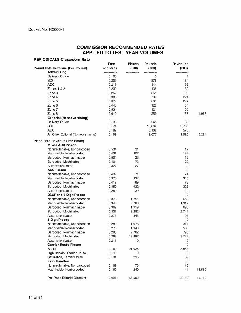
PERIODICALS-Classroom RateRate Pieces Pounds Revenues
Pound Rate Revenue (Per Pound) (dollars) (000) (000) (000) Advertising ----------- ----------- ----------- ----------- Delivery Off ice 0.160 5 1SCF 0.209 878 184ADC 0.219 144 32Zones 1 & 2 0.239 135 32Zone 3 0.257 351 90Zone 4 0.303 739 224Zone 5 0.372 609 227Zone 6 0.446 122 54Zone 7 0.534 121 65Zone 8 0.610 259 158 1,066Editorial (Nonadvertising)Delivery Off ice 0.133 245 33SCF 0.174 15,862 2,760ADC 0.182 3,162 576All Other Editorial (Nonadvertising) 0.199 9,677 1,926 5,294
Piece Rate Revenue (Per Piece)Mixed ADC PiecesNonmachinable, Nonbarcoded 0.534 31 17Machinable, Nonbarcoded 0.431 307 132Barcoded, Nonmachinable 0.504 23 12Barcoded, Machinable 0.404 73 29Automation Letter 0.327 27 9ADC Pieces 0Nonmachinable, Nonbarcoded 0.432 171 74Machinable, Nonbarcoded 0.370 932 345Barcoded, Nonmachinable 0.412 189 78Barcoded, Machinable 0.350 922 323Automation Letter 0.289 139 40DSCF and 3-Digit Pieces 0Nonmachinable, Nonbarcoded 0.373 1,751 653Machinable, Nonbarcoded 0.348 3,786 1,317Barcoded, Nonmachinable 0.362 1,919 695Barcoded, Machinable 0.331 8,282 2,741Automation Letter 0.275 345 955-Digit Pieces 0Nonmachinable, Nonbarcoded 0.289 1,078 311Machinable, Nonbarcoded 0.276 1,948 538Barcoded, Nonmachinable 0.285 2,782 793Barcoded, Machinable 0.268 13,887 3,722Automation Letter 0.211 0 0Carrier Route Pieces 0Basic 0.169 21,026 3,553High Density, Carrier Route 0.149 0 0Saturation, Carrier Route 0.131 295 39Firm Bundles 0Nonmachinable, Nonbarcoded 0.169 78 13Machinable, Nonbarcoded 0.169 240 41 15,569
Per-Piece Editorial Discount (0.091) 56,592 (5,150) (5,150)
COMMISSION RECOMMENDED RATES APPLIED TO TEST YEAR VOLUMES
14 of 51

Appendix GSchedule 2
PERIODICALS-Classroom Rate (continued)Rate Bundles Sacks Pallets Revenues
(dollars) (000) (000) (000) (000) Bundle Rate Revenue (Per Bundle) ----------- ----------- ----------- ----------- -----------
Mixed ADC SackMiXed ADC Bundle 0.100 44 4ADC Bundle 0.129 86 113-Digit/SCF Bundle 0.134 89 125-Digit Bundle 0.161 23 4Firm Bundle 0.079 115 9ADC Sack or PalletADC Bundle 0.038 81 33-Digit/SCF Bundle 0.063 365 235-Digit Bundle 0.095 282 27Carrier Route Bundle 0.104 73 8Firm Bundle 0.048 105 53-Digit/SCF Sack or Pallet3-Digit/SCF Bundle 0.039 571 225-Digit Bundle 0.084 991 83Carrier Route Bundle 0.095 1,282 122Firm Bundle 0.045 86 45-Digit Sack or Pallet5-Digit Bundle 0.008 50 0Carrier Route Bundle 0.039 269 10Firm Bundle 0.027 16 0 348
Sack Rate Revenue (Per Sack)Mixed ADC SackOSCF Entry 0.42 21 9OADC Entry 0.42 28 12ADC SackOSCF Entry 1.80 48 86OADC Entry 1.80 41 74OBMC Entry 1.80 10 18DBMC Entry 1.10 0.2 0DADC Entry 0.60 1 13-Digit/SCF SackOSCF Entry 1.90 110 209OADC Entry 1.90 116 220OBMC Entry 1.90 27 51DBMC Entry 1.20 1 1DADC Entry 1.00 2 2DSCF Entry 0.60 6 35-Digit/Carrier Route SackOSCF Entry 2.24 18 40OADC Entry 2.24 30 68OBMC Entry 2.24 8 17DBMC Entry 1.50 0.4 1DADC Entry 1.30 1 1DSCF Entry 0.90 3 2DDU Entry 0.70 0.2 0 814
COMMISSION RECOMMENDED RATES APPLIED TO TEST YEAR VOLUMES
15 of 51

Docket No. R2006-1
PERIODICALS-Classroom Rate (continued)Rate Bundles Sacks Pallets Revenues
(dollars) (000) (000) (000) (000) Pallet Rate Revenue (per pallet) ----------- ----------- ----------- ----------- -----------
ADC PalletOSCF Entry 18.61 2 34OADC Entry 18.61 2 35OBMC Entry 18.61 0.05 1DBMC Entry 13.00 0.05 1DADC Entry 8.90 2 203-Digit/SCF PalletOSCF Entry 22.98 2 41OADC Entry 22.98 2 44OBMC Entry 22.98 0.1 2DBMC Entry 14.40 0.1 2DADC Entry 12.20 2 20DSCF Entry 6.70 9 595-Digit PalletOSCF Entry 26.95 1 15OADC Entry 26.95 1 17OBMC Entry 26.95 0.01 0DBMC Entry 17.50 0.04 1DADC Entry 15.50 0.2 3DSCF Entry 8.00 3 20DDU Entry 1.20 0.01 0 312
Total Revenue 18,254Postage Not Receiving 5% Discount 1,066Postage Receiving 5% Discount 17,188Discount (5%) (859)
Pieces(000)
----------- Ride-Along Revenue 0.155 125 19
Total Postage Revenue 17,414
Times Correction Factor 1.0008 17,428
Fees Address Correction 138Periodicals Application Fee 5
Total Fees 143-------------------
TOTAL PERIODICALS-Classroom Rate 17,571
COMMISSION RECOMMENDED RATES APPLIED TO TEST YEAR VOLUMES
16 of 51

Appendix GSchedule 2
Standard M ail Re gular Subclas s
Unit Rate ($)TYAR
Volum e Re ve nue Nonautom ation (Pre sort) Cate goryLe tters , Nonm achinable
MADC per piece 0.520 29,688,185 15,437,856$ADC per piece 0.440 4,862,122 2,139,334 3-Digit per piece 0.411 61,251,859 25,174,514 5-Digit per piece 0.328 17,191,863 5,638,931 Subtotal 112,994,028 48,390,635
Le tters , M achinableMADC per piece 0.255 645,072,043 164,493,371ADC per piece 0.246 982,612,518 241,722,679 Subtotal 1,627,684,560 406,216,050
Flats , Pie ce -Rate dMADC per piece 0.515 71,729,651 36,940,770 ADC per piece 0.461 49,517,692 22,827,656 3-Digit per piece 0.427 126,959,031 54,211,506 5-Digit per piece 0.363 121,908,649 44,252,840 Subtotal 370,115,023 158,232,772
Parce ls , Pie ce -RatedMADC per piece 1.129 1,782,922 2,012,919 ADC per piece 0.914 22,101,690 20,200,945 3-Digit per piece 0.653 19,966,366 13,038,037 5-Digit per piece 0.607 2,218,485 1,346,620 SubTotal 46,069,463 36,598,521
Not Flat-M achinable , Piece-Rate dMADC per piece 1.028 4,472,727 4,597,963 ADC per piece 0.767 9,111,394 6,988,439 3-Digit per piece 0.506 61,328,539 31,032,241 5-Digit per piece 0.460 75,985,418 34,953,292 Subtotal 150,898,077 77,571,935
Flats , Pound-RatedMADC per piece 0.365 60,124,966 21,945,612 ADC per piece 0.311 41,506,538 12,908,533 3-Digit per piece 0.277 99,411,293 27,536,928 5-Digit per piece 0.213 95,456,749 20,332,288 Subtotal 296,499,546 82,723,362
Not Flat-M achinable , Pound-Rate dMADC per piece 0.878 13,926,107 12,227,122 ADC per piece 0.617 28,368,879 17,503,598 3-Digit per piece 0.356 190,950,135 67,978,248 5-Digit per piece 0.310 236,585,220 73,341,418 Subtotal 469,830,341 171,050,387
Parce ls , Pound-Rate dMachinab leMixed BMC per piece 0.909 76,878,428 69,882,491 BMC per piece 0.716 215,833,500 154,536,7865-Digit Machinable per piece 0.346 73,857,060 25,554,543 Subtotal 366,568,988 249,973,820Nonmachinab leMADC per piece 0.979 2,280,748 2,232,853 ADC per piece 0.764 28,272,912 21,600,505 3-Digit per piece 0.503 25,541,363 12,847,306 5-Digit per piece 0.457 2,837,929 1,296,934 Subtotal 58,932,953 37,977,597CMM Pieces per piece 0.460 2,634,246 1,211,753
pieces > 3,502,227,226 1,269,946,831
COMMISSION RECOMMENDED RATESAPPLIED TO TEST YEAR VOLUMES
17 of 51

Docket No. R2006-1
Standard Mail Regular Subclass
Unit Rate ($)TYAR
Volume Revenue Nonautomation (Presort) Category (continued)
Flats, Pound-RatedMADC per pound 0.739 24,773,937 18,307,939 ADC per pound 0.739 16,884,294 12,477,493 3-Digit per pound 0.739 38,205,775 28,234,068 5-Digit per pound 0.739 36,767,657 27,171,298 Subtotal 116,631,663 86,190,799
Not Flat-Machinable, Pound-RatedMADC per pound 0.739 5,849,751 4,322,966 ADC per pound 0.739 11,965,830 8,842,748 3-Digit per pound 0.739 68,354,684 50,514,112 5-Digit per pound 0.739 84,690,738 62,586,456 Subtotal 170,861,003 126,266,282
Parcels, Pound-RatedMachinableMixed BMC per pound 0.739 44,052,655 32,554,912 BMC per pound 0.739 138,895,007 102,643,4105-Digit Machinable per pound 0.739 30,512,566 22,548,786 Subtotal 213,460,227 157,747,108NonmachinableMADC per pound 0.739 1,394,844 1,030,790 ADC per pound 0.739 15,697,055 11,600,124 3-Digit per pound 0.739 14,936,284 11,037,914 5-Digit per pound 0.739 1,659,587 1,226,435 Subtotal 33,687,769 24,895,261
pounds > 534,640,663 395,099,450
Dropship Discounts: Piece-Rated
BMC per piece (0.033) 513,347,408 (16,940,464) SCF per piece (0.042) 528,029,146 (22,177,224) DDU per piece (0.051) 235,535 (12,012) Subtotal 1,041,612,090 (39,129,701)
Pound-Rated BMC per pound (0.159) 148,746,305 (23,650,663) SCF per pound (0.203) 93,222,845 (18,924,238) DDU per pound (0.248) 12,830,825 (3,182,045) Subtotal 254,799,975 (45,756,945)
Rates pieces > 3,502,227,226 1,580,159,635
Fees1,301,1611,520,482
339 BPRS Permit 150,733
420,183Total Revenue - Presort Category 1,583,552,534
COMMISSION RECOMMENDED RATESAPPLIED TO TEST YEAR VOLUMES
Standard Mail Forw arding
Certf icate of Mailing Bulk Permit Address Correction
18 of 51

Appendix GSchedule 2
Standard Mail Regular SubclassUnit Rate ($) TYAR Volum e Revenue
Autom ation Category
Letters, Piece-RatedMADC per piece 0.252 2,336,936,902 588,908,099$ ADC per piece 0.238 2,628,338,118 625,544,472 3-Digit per piece 0.233 20,241,531,311 4,716,276,795 5-Digit per piece 0.218 23,646,781,113 5,154,998,283 Subtotal 48,853,587,444 11,085,727,649
Letters, Pound-RatedMADC per piece 0.103 5,065,594 521,756 ADC per piece 0.089 9,617,128 855,924 3-Digit per piece 0.084 55,519,453 4,663,634 5-Digit per piece 0.069 2,836,600 195,725 Subtotal 73,038,775 6,237,040
Flats, Piece-RatedMADC per piece 0.477 30,743,777 14,664,782 ADC per piece 0.424 120,166,140 50,950,444 3-Digit per piece 0.392 1,874,462,333 734,789,234 5-Digit per piece 0.335 3,562,506,811 1,193,439,782 Subtotal 5,587,879,061 1,993,844,241
Flats, Pound-RatedMADC per piece 0.328 27,254,890 8,939,604 ADC per piece 0.275 106,529,363 29,295,575 3-Digit per piece 0.243 1,867,632,451 453,834,685 5-Digit per piece 0.186 3,549,526,288 660,211,890 Subtotal 5,550,942,992 1,152,281,754
pieces > 60,065,448,272 14,238,090,685
Letters, Pound-RatedMADC per pound 0.739 1,072,174 792,337 ADC per pound 0.739 2,034,803 1,503,720 3-Digit per pound 0.739 11,747,998 8,681,771 5-Digit per pound 0.739 600,626 443,863 Subtotal 15,455,602 11,421,690
Flats, Pound-RatedMADC per pound 0.739 11,457,379 8,467,003 ADC per pound 0.739 44,734,420 33,058,736 3-Digit per pound 0.739 678,700,916 501,559,977 5-Digit per pound 0.739 1,231,926,185 910,393,451 Subtotal 1,966,818,900 1,453,479,167
pounds > 1,982,274,502 1,464,900,857
COMMISSION RECOMMENDED RATESAPPLIED TO TEST YEAR VOLUMES
19 of 51

Docket No. R2006-1
Standard Mail Regular SubclassUnit Rate ($) TYAR Volume Revenue
Automation Category (continued) Piece-Rated
BMC per piece (0.033) 19,143,096,158 (631,722,173) SCF per piece (0.042) 19,054,850,741 (800,303,731) DDU per piece (0.051) 0 - Subtotal 38,197,946,898 (1,432,025,904)
Pound-Rated BMC per pound (0.159) 599,963,404 (95,394,181) SCF per pound (0.203) 714,320,947 (145,007,152) DDU per pound (0.248) 0 - Subtotal 1,314,284,351 (240,401,333)
Rates automation pieces > 60,065,448,272 14,030,564,304presort pieces > 3,502,227,226pieces paid @ First-Class and Priority 21,863,649NSA volume adjustment (110,692,386)
63,478,846,761Fees
26,125,20130,528,803
6,812 3,026,4788,436,597
Total Revenue - Automation Category 14,098,688,195
15,610,723,93913,723,602
17,808Subtotal 15,624,465,349
1.00008454615,625,786,337
Plus Fees 71,516,790(25,108,467)
15,672,194,661
0.24654346
COMMISSION RECOMMENDED RATESAPPLIED TO TEST YEAR VOLUMES
Standard Mail Forw arding
Address Correction
Certficate of Mailing Bulk Permit
BPRS Permit
Regular Subclass TotalTotal Postage from PiecesPieces Paid at First-Class RatesPieces Paid at Priority Rates
Revenue Per Piece
Times Revenue Adjustment FactorAdjusted Revenue
NSA AdjustmentTotal Revenue
20 of 51
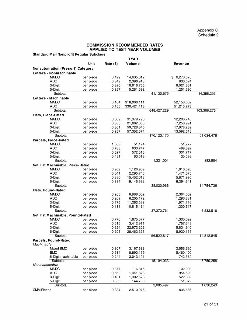
Appendix GSchedule 2
Standard Mail Nonprofit Regular Subclass
Unit Rate ($)TYAR
Volume Revenue Nonautom ation (Presort) CategoryLetters - Nonmachinable
MADC per piece 0.429 14,635,612 6,278,678$ ADC per piece 0.349 2,396,918 836,524 3-Digit per piece 0.320 18,816,755 6,021,361 5-Digit per piece 0.237 5,281,392 1,251,690 Subtotal 41,130,676 14,388,253
Letters - MachinableMADC per piece 0.164 318,006,111 52,153,002 ADC per piece 0.155 330,421,118 51,215,273 Subtotal 648,427,229 103,368,275
Flats, Piece-RatedMADC per piece 0.389 31,379,795 12,206,740 ADC per piece 0.335 21,662,660 7,256,991 3-Digit per piece 0.301 59,728,345 17,978,232 5-Digit per piece 0.237 57,352,374 13,592,513 Subtotal 170,123,175 51,034,476
Parcels, Piece-RatedMADC per piece 1.003 51,124 51,277 ADC per piece 0.788 633,747 499,392 3-Digit per piece 0.527 572,518 301,717 5-Digit per piece 0.481 63,613 30,598 Subtotal 1,321,001 882,984
Not Flat Machinable, Piece-RatedMADC per piece 0.902 1,126,969 1,016,526 ADC per piece 0.641 2,295,748 1,471,575 3-Digit per piece 0.380 15,452,618 5,871,995 5-Digit per piece 0.334 19,145,632 6,394,641 Subtotal 38,020,966 14,754,736
Flats, Pound-RatedMADC per piece 0.263 8,988,602 2,364,002 ADC per piece 0.209 6,205,172 1,296,881 3-Digit per piece 0.175 11,263,523 1,971,116 5-Digit per piece 0.111 10,815,464 1,200,517 Subtotal 37,272,761 6,832,516
Not Flat Machinable, Pound-RatedMADC per piece 0.776 1,675,377 1,300,092 ADC per piece 0.515 3,412,911 1,757,649 3-Digit per piece 0.254 22,972,206 5,834,940 5-Digit per piece 0.208 28,462,323 5,920,163 Subtotal 56,522,817 14,812,845
Parcels, Pound-RatedMachinable
Mixed BMC per piece 0.807 3,167,683 2,556,320 BMC per piece 0.614 8,893,159 5,460,400 5-Digit machinable per piece 0.244 3,043,191 742,539 Subtotal 15,104,033 8,759,258
Nonmachinab leMADC per piece 0.877 116,315 102,008 ADC per piece 0.662 1,441,878 954,523 3-Digit per piece 0.401 1,302,573 522,332 5-Digit per piece 0.355 144,730 51,379 Subtotal 3,005,497 1,630,243
CMM Pieces per piece 0.334 2,510,976 838,666
COMMISSION RECOMMENDED RATESAPPLIED TO TEST YEAR VOLUMES
21 of 51
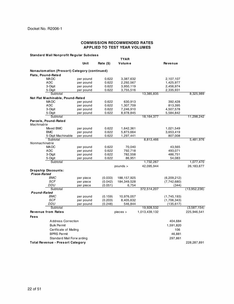
Docket No. R2006-1
Standard Mail Nonprofit Regular Subclass
Unit Rate ($)TYAR
Volum e Revenue
Nonautom ation (Presort) Category (continued)Flats , Pound-Rate d
MADC per pound 0.622 3,387,632 2,107,107 ADC per pound 0.622 2,292,567 1,425,977 3-Digit per pound 0.622 3,950,119 2,456,974 5-Digit per pound 0.622 3,755,516 2,335,931 Subtotal 13,385,835 8,325,989
Not Flat M achinable , Pound-RatedMADC per pound 0.622 630,913 392,428 ADC per pound 0.622 1,307,709 813,395 3-Digit per pound 0.622 7,246,910 4,507,578 5-Digit per pound 0.622 8,978,845 5,584,842 Subtotal 18,164,377 11,298,242
Parce ls , Pound-RatedMachinab le
Mixed BMC per pound 0.622 1,642,361 1,021,549 BMC per pound 0.622 5,873,664 3,653,419 5-Digit Machinable per pound 0.622 1,297,441 807,008 Subtotal 8,813,466 5,481,976
Nonmachinab leMADC per pound 0.622 70,040 43,565 ADC per pound 0.622 792,718 493,071 3-Digit per pound 0.622 782,558 486,751 5-Digit per pound 0.622 86,951 54,083 Subtotal 1,732,267 1,077,470
pounds > 42,095,944 26,183,677Dropship Discounts: Piece-Rated
BMC per piece (0.033) 188,157,925 (6,209,212) SCF per piece (0.042) 184,349,528 (7,742,680) DDU per piece (0.051) 6,754 (344) Subtotal 372,514,207 (13,952,236)
Pound-Rated BMC per pound (0.159) 10,976,057 (1,745,193) SCF per pound (0.203) 8,405,632 (1,706,343) DDU per pound (0.248) 546,844 (135,617) Subtotal 19,928,532 (3,587,154)
pieces > 1,013,439,132 225,946,541
Fees404,684
1,591,820106
46,881297,861
Total Revenue - Pres ort Category 228,287,891
COMMISSION RECOMMENDED RATESAPPLIED TO TEST YEAR VOLUMES
BPRS Permit Standard Mail Forw arding
Revenue from Rates
Address Correction Bulk Permit Certf icate of Mailing
22 of 51

Appendix GSchedule 2
Standard Mail Nonprofit Regular SubclassUnit Rate ($) TYAR Volume Revenue
Automation Category
Letters, Piece-RatedMADC per piece 0.161 897,990,192 144,576,421$ ADC per piece 0.147 855,332,716 125,733,909 3-Digit per piece 0.142 4,530,178,577 643,285,358 5-Digit per piece 0.127 3,446,662,686 437,726,161 Subtotal 9,730,164,171 1,351,321,849
Letters, Pound-RatedMADC per piece 0.035 420,059 14,702 ADC per piece 0.021 362,033 7,603 3-Digit per piece 0.016 2,607,354 41,718 5-Digit per piece 0.001 160,882 161 Subtotal 3,550,329 64,183
Flats, Piece-RatedMADC per piece 0.354 9,146,821 3,237,975 ADC per piece 0.301 35,751,568 10,761,222 3-Digit per piece 0.269 388,908,744 104,616,452 5-Digit per piece 0.212 739,139,979 156,697,675 Subtotal 1,172,947,112 275,313,324
Flats, Pound-RatedMADC per piece 0.228 2,096,479 477,997 ADC per piece 0.175 8,194,368 1,434,014 3-Digit per piece 0.143 167,441,459 23,944,129 5-Digit per piece 0.086 318,230,634 27,367,835 Subtotal 495,962,940 53,223,975
pieces > 11,402,624,552 1,679,923,332
Letters, Pound-RatedMADC per pound 0.622 89,309 55,550 ADC per pound 0.622 76,960 47,869 3-Digit per pound 0.622 551,679 343,145 5-Digit per pound 0.622 34,035 21,170 Subtotal 751,983 467,734
Flats, Pound-RatedMADC per pound 0.622 792,054 492,657 ADC per pound 0.622 3,089,605 1,921,734 3-Digit per pound 0.622 53,423,927 33,229,682 5-Digit per pound 0.622 98,095,820 61,015,600 Subtotal 155,401,405 96,659,674
pounds > 156 153 389 97 127 408
COMMISSION RECOMMENDED RATESAPPLIED TO TEST YEAR VOLUMES
23 of 51
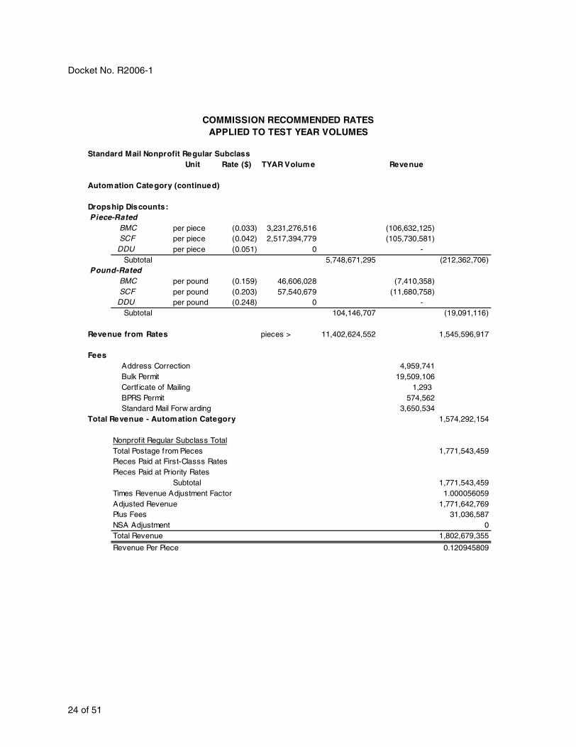
Docket No. R2006-1
Standard Mail Nonprofit Regular SubclassUnit Rate ($) TYAR Volume Revenue
Automation Category (continued)
Dropship Discounts: Piece-Rated
BMC per piece (0.033) 3,231,276,516 (106,632,125) SCF per piece (0.042) 2,517,394,779 (105,730,581) DDU per piece (0.051) 0 - Subtotal 5,748,671,295 (212,362,706)
Pound-Rated BMC per pound (0.159) 46,606,028 (7,410,358) SCF per pound (0.203) 57,540,679 (11,680,758) DDU per pound (0.248) 0 - Subtotal 104,146,707 (19,091,116)
pieces > 11,402,624,552 1,545,596,917
Fees4,959,741
19,509,1061,293
574,5623,650,534
1,574,292,154
Nonprofit Regular Subclass TotalTotal Postage from Pieces 1,771,543,459Pieces Paid at First-Classs RatesPieces Paid at Priority Rates
Subtotal 1,771,543,459Times Revenue Adjustment Factor 1.000056059Adjusted Revenue 1,771,642,769Plus Fees 31,036,587NSA Adjustment 0Total Revenue 1,802,679,355
Revenue Per Piece 0.120945809
COMMISSION RECOMMENDED RATESAPPLIED TO TEST YEAR VOLUMES
Standard Mail Forw arding
Revenue from Rates
Total Revenue - Automation Category
Address Correction Bulk Permit Certf icate of Mailing BPRS Permit
24 of 51

Appendix GSchedule 2
Standard Mail ECR Subclass
Unit Rates Volume Revenue (1) (2) (3)
LettersLetters, Piece-Rated
Basic per piece 0.226 1,787,135,617 403,892,649 High Density per piece 0.186 547,975,921 101,923,521 Saturation per piece 0.177 3,217,068,446 569,421,115 Subtotal 5,552,179,984 1,075,237,286
Letters, Pound-Rated Basic per piece 0.098 3,955,159 387,606 High Density per piece 0.058 12,957,244 751,520 Saturation per piece 0.049 108,795,396 5,330,974 Subtotal 125,707,799 6,470,100
Letters, Pound-Rated Basic per pound 0.621 1,173,207 728,562 High Density per pound 0.621 3,331,764 2,069,025 Saturation per pound 0.621 25,866,498 16,063,095 Subtotal 30,371,469 18,860,682
FlatsFlats, Piece-Rated
Basic per piece 0.249 5,683,719,730 1,415,246,213 High Density per piece 0.205 856,776,680 175,639,219 Saturation per piece 0.187 7,181,961,242 1,343,026,752 Subtotal 13,722,457,653 2,933,912,185
Flats, Pound-Rated Basic per piece 0.121 5,602,090,986 677,853,009 High Density per piece 0.077 999,100,723 76,930,756 Saturation per piece 0.059 3,679,961,470 217,117,727 Subtotal 10,281,153,179 971,901,492
ParcelsParcels, Piece-Rated
Basic per piece 0.499 207,573 103,579 High Density per piece 0.378 7,338 2,774 Saturation per piece 0.369 33,757 12,456 Subtotal 248,668 118,809
Parcels, Pound-Rated Basic per piece 0.371 253,593 94,083 High Density per piece 0.250 10,938 2,734 Saturation per piece 0.241 95,687 23,061 Subtotal 360,218 119,878
pieces > 29,682,107,501 4,987,759,749 NSA Adjustment (4,866,935)
Nonletter Pounds Basic per pound 0.621 1,777,210,500 1,103,647,721 High Density per pound 0.621 373,403,588 231,883,628 Saturation per pound 0.621 1,149,187,090 713,645,183 Subtotal 3,299,801,179 2,049,176,532
pounds > 3,330,172,648 2,068,037,214
COMMISSION RECOMMENDED RATESAPPLIED TO TEST YEAR VOLUMES
25 of 51
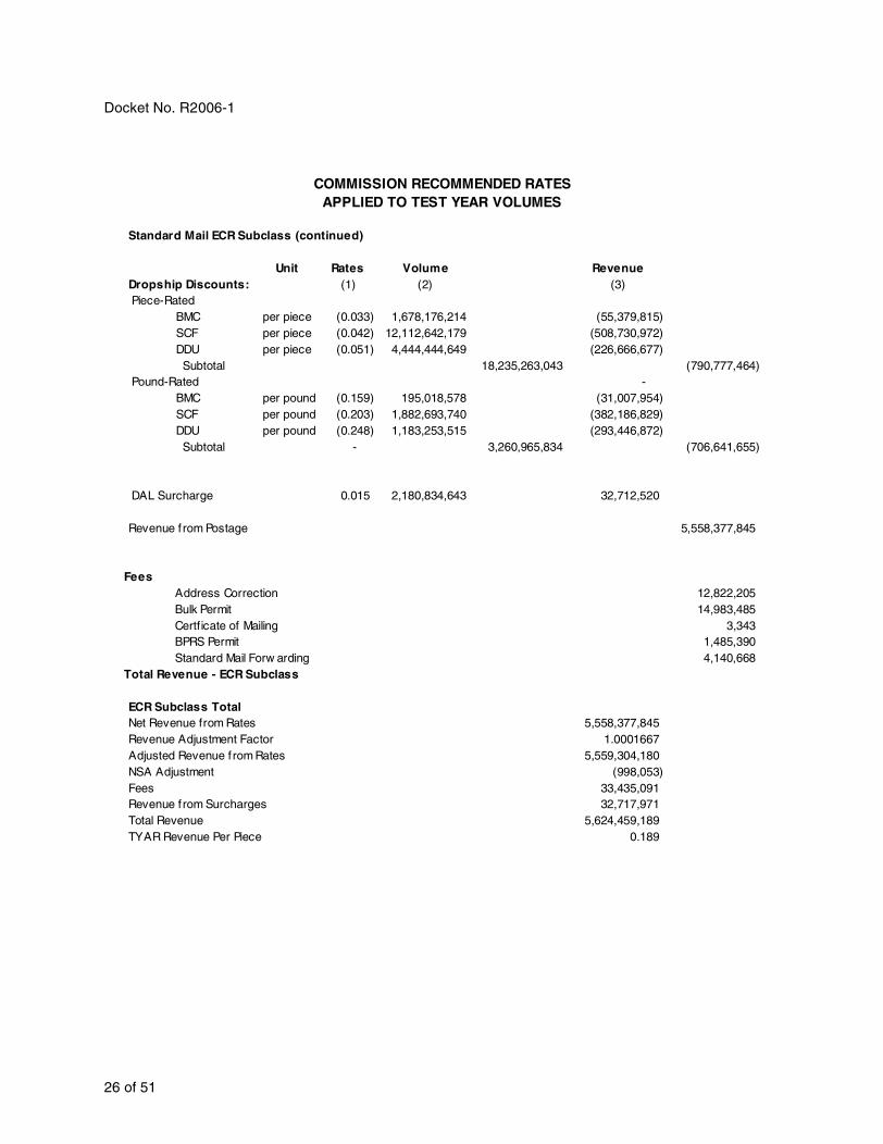
Docket No. R2006-1
Standard Mail ECR Subclass (continued)
Unit Rates Volume RevenueDropship Discounts: (1) (2) (3) Piece-Rated
BMC per piece (0.033) 1,678,176,214 (55,379,815) SCF per piece (0.042) 12,112,642,179 (508,730,972) DDU per piece (0.051) 4,444,444,649 (226,666,677) Subtotal 18,235,263,043 (790,777,464)
Pound-Rated - BMC per pound (0.159) 195,018,578 (31,007,954) SCF per pound (0.203) 1,882,693,740 (382,186,829) DDU per pound (0.248) 1,183,253,515 (293,446,872) Subtotal - 3,260,965,834 (706,641,655)
DAL Surcharge 0.015 2,180,834,643 32,712,520
Revenue from Postage 5,558,377,845
Fees12,822,205 14,983,485
3,343 1,485,390 4,140,668
Total Revenue - ECR Subclass
ECR Subclass Total5,558,377,845
1.0001667 5,559,304,180
(998,053) Fees 33,435,091
32,717,971 5,624,459,189
0.189
COMMISSION RECOMMENDED RATESAPPLIED TO TEST YEAR VOLUMES
Address Correction Bulk Permit Certficate of Mailing BPRS Permit Standard Mail Forw arding
Net Revenue from RatesRevenue Adjustment FactorAdjusted Revenue from RatesNSA Adjustment
Revenue from SurchargesTotal RevenueTYAR Revenue Per Piece
26 of 51

Appendix GSchedule 2
Standard Mail Nonprofit ECR Subclass
Unit Rates Volume Revenue (1) (2) (3)
LettersLetters - Piece Rated
Basic per piece 0.157 265,215,375 41,638,814 High Density per piece 0.117 57,737,495 6,755,287 Saturation per piece 0.108 634,654,437 68,542,679 SubTotal 957,607,307 116,936,780
Letters - Pound Rated Basic per piece 0.068 420,425 28,589 High Density per piece 0.028 60,600 1,697 Saturation per piece 0.019 4,913,382 93,354 SubTotal 5,394,407 123,640
Letters - Pound Rated Basic per pound 0.432 107,612 46,488 High Density per pound 0.432 14,491 6,260 Saturation per pound 0.432 1,152,734 497,981 SubTotal 1,274,837 550,730
FlatsFlats, Piece-Rated
Basic per piece 0.180 941,623,274 169,492,189 High Density per piece 0.136 65,048,477 8,846,593 Saturation per piece 0.118 339,376,598 40,046,439 SubTotal 1,346,048,349 218,385,221
Flats, Pound-Rated Basic per piece 0.091 152,468,834 13,874,664 High Density per piece 0.047 1,297,297 60,973 Saturation per piece 0.029 66,417,782 1,926,116 SubTotal 220,183,912 15,861,752
ParcelsParcels, Piece-Rated
Basic per piece 0.430 17,916 7,704 High Density per piece 0.309 - - Saturation per piece 0.300 3,975 1,192 SubTotal 21,891 8,896
Parcels, Pound-Rated Basic per piece 0.341 49,699 16,947 High Density per piece 0.220 - - Saturation per piece 0.211 19,603 4,136 SubTotal 69,301 21,083
pieces > 2,529,325,167 351,337,373
Nonletter Pounds Basic per pound 0.432 46,552,707 20,110,769 High Density per pound 0.432 461,439 199,342 Saturation per pound 0.432 20,339,259 8,786,560 SubTotal 67,353,404 29,096,671
pounds > 68,628,241 29,647,400
COMMISSION RECOMMENDED RATESAPPLIED TO TEST YEAR VOLUMES
27 of 51

Docket No. R2006-1
Standard Mail Nonprofit ECR Subclass (continued)
Unit Rates Volume RevenueDropship Discounts: (1) (2) (3) Piece-Rated
BMC per piece (0.033) 272,740,868 (9,000,449) SCF per piece (0.042) 1,606,516,552 (67,473,695) DDU per piece (0.051) 117,661,155 (6,000,719) Subtotal 1,996,918,575 (82,474,863)
Pound-Rated BMC per pound (0.159) 6,249,923 (993,738) SCF per pound (0.203) 46,709,058 (9,481,939) DDU per pound (0.248) 6,709,289 (1,663,904) Subtotal - 59,668,270 (12,139,580)
DAL Surcharge 0.015 81,478,329 1,222,175
Revenue from Postage 286,370,330
Fees1,092,808 4,298,553
285 126,596 804,343
Total Revenue - Nonprofit ECR
Nonprofit ECR Subclass Total286,370,330
1.0001667 286,418,055
Fees 6,322,585 1,222,379
293,963,019 0.116
Revenue from SurchargesTotal RevenueTYAR Revenue Per Piece
Standard Mail Forw arding
Net Revenue from RatesRevenue Adjustment FactorAdjusted Revenue from Rates
Address Correction Bulk Permit Certf icate of Mailing BPRS Permit
APPLIED TO TEST YEAR VOLUMESCOMMISSION RECOMMENDED RATES
28 of 51

29 of 51
App
endix GS
chedule 2
s Revenues
346 9,559,179 117 126,201,061 658 24,731,158 951 5,412,842 122 462,145 194 166,366,384
164,950,345
527,958 22,006,534 1,579,613
34,075,751 58,189,856
1,397,485,297
1,156,532
58,105,921
1,456,747,748
COMMISSION RECOMMENDED RATESAPPLIED TO TEST YEAR VOLUMES
Package Service - Parcel Post
Pieces Revenues PieceInter-BMC Intra-BMC
Zones 1 & 2 2,690,662 15,921,608 Zones Local 2,316, 3 5,398,937 36,569,486 1 & 2 24,528, 4 17,715,446 130,743,834 3 4,236, 5 21,002,167 165,647,568 4 916, 6 10,669,354 88,687,685 5 66, 7 7,866,288 68,773,195 Subtotal 32,064, 8 13,062,940 127,584,637 Times Revenue Adjustment
Subtotal 78,405,794 633,928,014 Times Revenue Adjustment 631,017,543
Pieces RevenuesParcel Select Other Postage Revenue
DBMC Zone 1 & 2 43,416,181 149,759,303 Pickup Fees3 10,926,575 53,789,667 Alaska Bypass4 2,353,134 13,810,440 Parcel Enclosures5 - - PRS
DSCF 1,725,069 4,474,609 SubtotalDDU 191,573,847 314,525,135
Subtotal 249,994,806 536,359,154 Times Revenue Adjustment 543,327,552 Total Postage Revenue
FeesAddress Correction 639,066 Bulk Permit 28,289 Certificate of Mailing 24,003 Special Handling 339,395 Parcel Air Lift 59,589 Shipper Paid Forwarding 1,532 Merchandise Return 64,658
Total Fees 1,156,532
Adjustments to RevenueDim-Weight Adjustment 10,255,936Barcode Discount (266,162) BMC Presort Discount (389,019) OBMC Entry Discount (17,865,644) Nonmachinable Surcharge 66,370,810
Total Adjustments to Revenue 58,105,921
TOTAL PARCEL POST
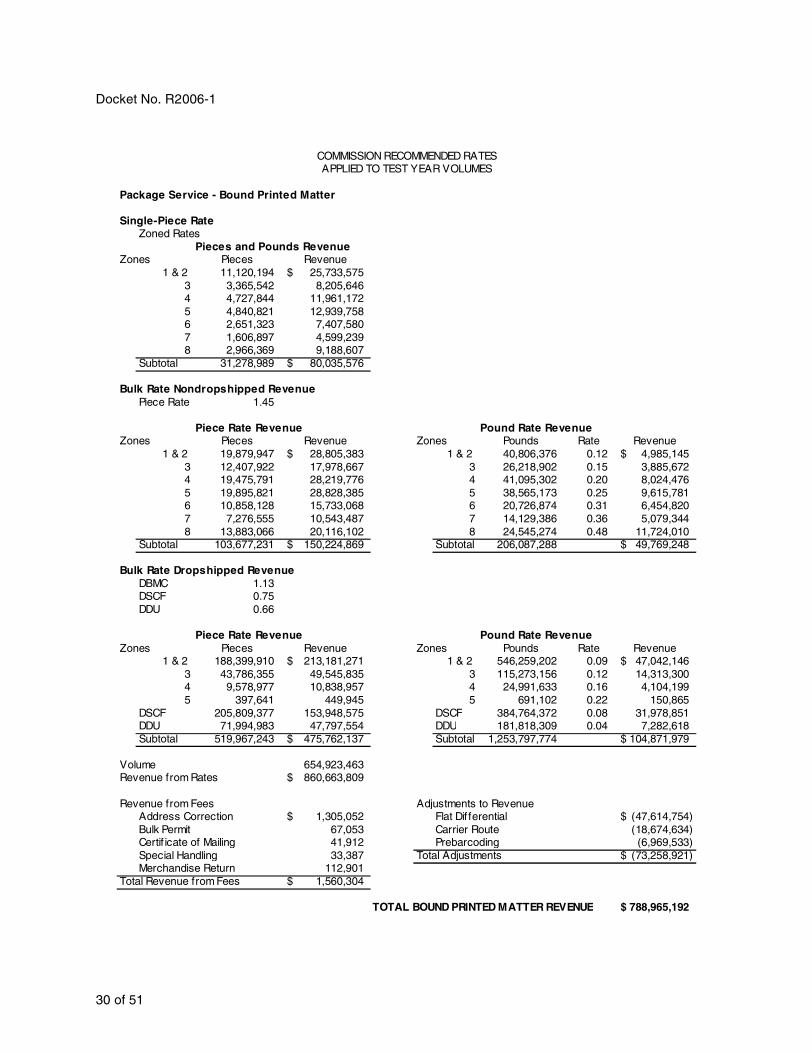
Docket No. R2006-1
APPLIED TO TEST YEAR VOLUMES
Package Service - Bound Printed Matter
Single-Piece RateZoned Rates
Pieces and Pounds RevenueZones Pieces Revenue
1 & 2 11,120,194 25,733,575$ 3 3,365,542 8,205,646 4 4,727,844 11,961,172 5 4,840,821 12,939,758 6 2,651,323 7,407,580 7 1,606,897 4,599,239 8 2,966,369 9,188,607
Subtotal 31,278,989 80,035,576$
Bulk Rate Nondropshipped RevenuePiece Rate 1.45
Piece Rate Revenue Pound Rate RevenueZones Pieces Revenue Zones Pounds Rate Revenue
1 & 2 19,879,947 28,805,383$ 1 & 2 40,806,376 0.12 4,985,145$ 3 12,407,922 17,978,667 3 26,218,902 0.15 3,885,672 4 19,475,791 28,219,776 4 41,095,302 0.20 8,024,476 5 19,895,821 28,828,385 5 38,565,173 0.25 9,615,781 6 10,858,128 15,733,068 6 20,726,874 0.31 6,454,820 7 7,276,555 10,543,487 7 14,129,386 0.36 5,079,344 8 13,883,066 20,116,102 8 24,545,274 0.48 11,724,010
Subtotal 103,677,231 150,224,869$ Subtotal 206,087,288 49,769,248$
Bulk Rate Dropshipped RevenueDBMC 1.13 DSCF 0.75 DDU 0.66
Piece Rate Revenue Pound Rate RevenueZones Pieces Revenue Zones Pounds Rate Revenue
1 & 2 188,399,910 213,181,271$ 1 & 2 546,259,202 0.09 47,042,146$ 3 43,786,355 49,545,835 3 115,273,156 0.12 14,313,300 4 9,578,977 10,838,957 4 24,991,633 0.16 4,104,199 5 397,641 449,945 5 691,102 0.22 150,865
DSCF 205,809,377 153,948,575 DSCF 384,764,372 0.08 31,978,851 DDU 71,994,983 47,797,554 DDU 181,818,309 0.04 7,282,618 Subtotal 519,967,243 475,762,137$ Subtotal 1,253,797,774 104,871,979$
Volume 654,923,463 Revenue from Rates 860,663,809$
Revenue from Fees Adjustments to RevenueAddress Correction 1,305,052$ Flat Dif ferential (47,614,754)$ Bulk Permit 67,053 Carrier Route (18,674,634) Certif icate of Mailing 41,912 Prebarcoding (6,969,533) Special Handling 33,387 Total Adjustments (73,258,921)$ Merchandise Return 112,901
Total Revenue from Fees 1,560,304$
TOTAL BOUND PRINTED MATTER REVENUE 788,965,192$
COMMISSION RECOMMENDED RATES
30 of 51

Appendix GSchedule 2
Package Services - Media and Library Rate
Revenue from RatesMedia Mail Library Rate Combined
Single-PieceFirst Pound Barcoded 31,229,589$ 1,997,404$ 33,226,993$ Non-Barcoded 229,748,492 21,680,956 251,429,448 Pounds 2-7 47,441,344 4,127,007 51,568,351 Pounds 8-70 8,030,905 638,145 8,669,051 Total Non-Presorted 316,450,330$ 28,443,513$ 344,893,843$ Times revenue adjustment 321,682,496$ 29,436,623$ 351,119,119$
PresortedFirst Pound - Presort Level A (5-Digit) 2,081,601$ 95,358$ 2,176,959$ First Pound - Presort Level B (BMC) Barcoded 42,557,407 10,086 42,567,493 Non-Barcoded 9,530,743 910,494 10,441,237 Pounds 2-7 12,231,244 200,393 12,431,637 Pounds 8-70 675,416 16,349 691,765 Total Presorted 67,076,412$ 1,232,679$ 68,309,091$ Times revenue adjustment 68,314,340$ 1,338,308$ 69,652,648$
Total Revenue from Postage 389,996,836$ 30,774,930$ 420,771,766$
Revenue from FeesAddress Correction 281,809$ 51,238$ 333,047$ Bulk Permit 123,358 123,358 Certificate of Mailing 9,834 790 10,625 Special Handling 37,272 37,272 Merchandise Return 26,492 2,129 28,621
Total Revenue from Fees 478,765$ 54,158$ 532,923$
Total Media and Library Rate Revenue 390,475,601$ 30,829,088$ 421,304,689$
COMMISSION RECOMMENDED RATESAPPLIED TO TEST YEAR VOLUMES
31 of 51

32 of 51
Docket N
o. R2006-1Manual
ctions Fee Revenues 00) (000)
87,684 $0.50 11,712,14965,399 $0.50 505,34178,311 $0.50 747,78760,116 $0.50 121,60199,023 $0.50 20,428,59668,165 $0.50 1,342,84258,699 $0.50 34,858,315
23,891 $0.50 61,946
49,674 $0.50 1,676,38180,570 $0.50 14,399,78106,603 $0.50 3,887,55153,459 $0.50 137,94290,306 $0.50 20,101,656
10,898 $0.50 1,705,84598,594 $0.50 31,084,94288,900 $0.50 13,915,01398,392 $0.50 46,705,799
4,478 $0.50 639,0662,590 $0.50 1,305,0521,059 $0.50 281,8091,105 $0.50 51,2389,232 2,277,165
80,520 104,004,881$
COMMISSION RECOMMENDED FEES
SPECIAL SERVICES
A. Address Correction FeesAutomated 1st 2 notices Automated add. Notices ElectronicTransactions Fee Transactions Fee Transactions Fee Transa
(000) (000) (000) (0First-Class
Regular: Single-Piece Letters 0 $0.00 0 $0.05 15,305,120 $0.06 21,5Presort Letters 9,237,507 $0.00 2,886,721 $0.05 471,751 $0.06 6Single-Piece Cards 0 $0.00 0 $0.05 977,188 $0.06 1,3Presort Cards 2,222,834 $0.00 694,636 $0.05 113,518 $0.06 1
Auto: Automation Letters 373,429,808 $0.00 116,696,815 $0.05 19,070,725 $0.06 26,8Automation Cards 24,546,828 $0.00 7,670,884 $0.05 1,253,584 $0.06 1,7 Total First-Class 409,436,977 - 127,949,055 $0.05 37,191,886 $0.06 52,4
Priority 0 $0.25 1
PeriodicalsIn County 5,406,176 $0.25 6Regular Rate 46,437,985 $0.25 5,5Nonprofit 12,536,999 $0.25 1,5Classroom 444,851 $0.25 Total Periodicals 64,826,010 $0.25 7,7
Standard MailPresort 13,818,738 0.02 4,935,263 $0.15 2,734,926 $0.25Automation 251,813,449 0.02 89,933,375 $0.15 49,837,479 $0.25 1ECR 112,722,980 0.02 40,258,207 $0.15 22,309,488 $0.25 Total Bulk Std. 378,355,167 0.02 135,126,845 $0.15 74,881,893 $0.25 2
Package ServicesParcel Post 2,547,310 $0.25BPM 5,215,027 $0.25Media Mail 1,125,119 $0.25Library Rate 202,742 $0.25 Total Pkg. Services 9,090,197
Grand Total Address Correction 787,792,143 263,075,900 185,989,987 60,6
Grand Total Trans. (Auto & Electronic & Manual) 1,297,538,550
APPLIED TO TEST YEAR TRANSACTIONS

Appendix GSchedule 2
B. Bulk/Presort Mailing Fees
Transactions Fee RevenuesFirst Class
Regular: Letter Presort 873 175$ 152,731$ Post Card Presort 210 175 36,752
Auto: Auto Letter 36,006 175 6,301,041 Auto Postcard 2,319 175 405,851
Total First-Class 39,408 6,896,374
StandardRegular: Presort 8,688 175 1,520,482
Automation 174,450 175 30,528,803 ECR 85,620 175 14,983,485 Total Reg. Bulk 268,759 47,032,770
Nonprofit: NP Presort 9,096 175 1,591,820 NP Automation 111,481 175 19,509,106 NP ECR 24,563 175 4,298,553 Total NP Bulk 145,140 25,399,479
Total Standard 413,899 72,432,249
Package Services705 175 123,358
2 175 350
153 175 26,839 383 175 67,053 537 93,892
1,243 217,600
Merchandise ReturnFirst-Class 457 175 80,054 Priority 222 175 38,889 Standard - 175 - Package Services 355 175 62,147
Total Merchandise Return 1,035 181,090
Bulk Parcel Return Service 121 175 21,179
Total Bulk/Presort Mailing Fees 455,704 79,748,143$
COMMISSION RECOMMENDED FEESAPPLIED TO TEST YEAR TRANSACTIONS
Total Destination Entry
Total Package Services
Bound Printed Matter Parcel SelectDestination Entry Parcel Return Service Media Mail
33 of 51

Docket No. R2006-1
C. Business Reply Mail FeesVolume Revenues
(000) Fee (000)Advance Deposit QBRM with Quarterly Fee 151,803 0.005$ 759$ QBRM without Quarterly Fee 206,021 0.050 10,301$ Total QBRM 357,824 11,060$
Non-QBRM Advance Deposit 305,860 0.080 24,469$ Nonletter-Size 3,582 0.011 39$ Priority 2,869 0.080 230$
Subtotal - Per Piece 670,135 35,798$
Account Maintenance Fee 65 550 35,802$ Nonletter-Size Monthly Fee 0.02 900 234$ QBRM Quarterly Fee 1 1,800 7,663$ Permit Fee 122 175 21,288$
Subtotal - Fees 188 64,987$
Advance Total 670,135 100,785$
Nonadvance Deposit First-Class 135,590 0.700 94,913$ Priority 1,196 0.700 837$ Nonadvance Total 136,785 95,750$
Grand Total 806,920 196,535$
COMMISSION RECOMMENDED FEESAPPLIED TO TEST YEAR TRANSACTIONS
34 of 51

Appendix GSchedule 2
D. Certificate of Mailing Fees
TRANSACTIONS Basic Firm Book First Additional Subclass Class1000 1000 Total Total
First-Class Regular: Letter 1,879,726 340,196 - - 2,219,922 Letter Presort - - 946 2,180 3,126 Postcard 120,015 21,721 - - 141,736 Postcard Presort - - 228 524 752
First-Class Auto: Auto Letter - - 38,253 88,109 126,362 Auto Postcard - - 2,515 5,792 8,306 2,500,204
Priority 50,919 1,861 558 260 53,598 53,598
Standard Regular: Presort 203 - 23 - 226 Automation 3,919 - 437 - 4,356 ECR 2,200 - 245 - 2,445
Standard Nonprofit: Presort 93 - 10 - 103 Automation 731 - 81 - 812 ECR 179 - 20 - 199 8,140
Package Services: Parcels 22,752 323 - - 23,075 BPM 39,728 565 - - 40,293 Media Mail 9,322 133 - - 9,454 Library Rate 749 11 - - 760 73,583
Totals 2,130,536 364,809 43,315 96,864 2,635,524 2,635,524
Basic Firm Book First Additional Subclass ClassREVENUES 1000 1000 Total Total
Fee >> $1.05 $0.35 $5.50 $0.60
First-Class Regular: Letter $1,973,713 $119,069 $0 $0 $2,092,781Letter Presort - - 5,204 1,308 $6,512Postcard 126,016 7,602 - - $133,618Postcard Presort - - 1,252 315 $1,567
First-Class Auto: Auto Letter - - 210,392 52,865 $263,257Auto Postcard - - 13,830 3,475 $17,305 $2,515,040
- - - -
Priority 53,465 651 3,067 156 $57,340 57,340- - - -
Standard Regular: Standard Presort 213 - 124 - $338Automation 4,115 - 2,402 - $6,516ECR 2,310 - 1,348 - $3,658
Standard Nonprofit: Standard Presort 98 - 57 - $155Automation 767 - 448 - $1,215ECR 188 - 109 - $297 12,179
- - - - Package Services: Parcel Post 23,890 113 - - $24,003
BPM 41,714 198 - - $41,912Media Mail 9,788 46 - - $9,834Library Rate 787 4 - - $790 76,540
Totals $2,237,063 $127,683 $238,234 $58,119 $2,661,098 $2,661,098
COMMISSION RECOMMENDED FEESAPPLIED TO TEST YEAR TRANSACTIONS
35 of 51

Docket No. R2006-1
E. Certified Mail Fees Transactions Revenues(000) Fee (000)
Basic Fee 262,526 2.65$ 695,695$
COMMISSION RECOMMENDED FEESAPPLIED TO TEST YEAR TRANSACTIONS
F. Collect on Delivery FeesTransactions Revenues
Value (000) Fee (000) Fee Charge for Collectable Amount or Insurance Coverage up to 50$ 321 5.10$ 1,639$
100 259 6.25 1,619$ 200 369 7.40 2,728$ 300 137 8.55 1,172$ 400 40 9.70 388$ 500 18 10.85 197$ 600 12 12.00 141$ 700 5 13.15 60$ 800 5 14.30 70$ 900 0 15.45 1$
1,000 5 16.60 80$
1,171 8,096$
Registered COD 3 4.55 12$ Notice of Non-Delivery 44 3.40 149$ Alteration of COD 0 3.40 -$ Restricted Delivery 0 4.10 -$
1,173 8,258$ Total Collect on Delivery
Additional Services -- Only Restricted Delivery from Other Subservices
Total Before Additional Services
36 of 51

Appendix GSchedule 2
G. InsuranceValue Transactions Fee Revenues
Domestic Liability up to 50$ 19,580,597 1.65$ 32,307,985$ 100 11,435,031 2.05 23,441,814 200 6,251,921 2.45 15,317,207 300 1,778,424 4.60 8,180,752 400 803,689 5.50 4,420,287 500 746,224 6.40 4,775,836 600 286,296 7.30 2,089,963 700 189,188 8.20 1,551,338 800 142,777 9.10 1,299,273 900 56,847 10.00 568,474
1,000 182,600 10.90 1,990,336 1,100 27,812 11.80 328,183 1,200 34,264 12.70 435,150 1,300 15,702 13.60 213,549 1,400 28,892 14.50 418,930 1,500 58,048 15.40 893,932 1,600 8,954 16.30 145,948 1,700 4,277 17.20 73,561 1,800 6,165 18.10 111,583 1,900 3,274 19.00 62,203 2,000 42,064 19.90 837,075 2,100 1,334 20.80 27,738 2,200 1,173 21.70 25,451 2,300 1,007 22.60 22,751 2,400 3,718 23.50 87,367 2,500 9,109 24.40 222,254 2,600 636 25.30 16,091 2,700 1,536 26.20 40,234 2,800 2,428 27.10 65,807 2,900 868 28.00 24,316 3,000 24,754 28.90 715,399 3,100 835 29.80 24,875 3,200 1,171 30.70 35,943 3,300 0 31.60 - 3,400 270 32.50 8,783 3,500 1,818 33.40 60,735 3,600 3,715 34.30 127,420 3,700 54 35.20 1,883 3,800 0 36.10 - 3,900 569 37.00 21,068 4,000 3,612 37.90 136,889 4,100 10,518 38.80 408,091 4,200 0 39.70 - 4,300 1,021 40.60 41,446 4,400 0 41.50 - 4,500 616 42.40 26,107 4,600 0 43.30 - 4,700 31 44.20 1,375 4,800 0 45.10 - 4,900 222 46.00 10,234 5,000 10,153 46.90 476,153
Total 41,764,212 102,091,792$ Express Mail Insurance 433,843 1,417,275Grand Total 42,198,055 103,509,067$
COMMISSION RECOMMENDED FEESAPPLIED TO TEST YEAR TRANSACTIONS
37 of 51

Docket No. R2006-1
Transactions Fee Revenues
Account Maintenance Fee 763 550$ 419,696$
Transactions First-Class 10,298,235 - - Priority 5,002,742 - - Standard 0 - - Package Services 7,994,655 - - Total Transactions 23,295,632 -
419,696$
COMMISSION RECOMMENDED FEES
APPLIED TO TEST YEAR TRANSACTIONS
H. Merchandise Return
Total Merchandise Return
Transactions Fee Revenues (000) (000)
APO-FPO 304 0.30$ 91$
Domestic (up to $500) 136,376 1.05 143,195$
Domestic ($500 to $1000) 17,475 1.50 26,212$
Inquiry Fees 551 5.00 2,757$
Subtotal 154,155 172,256$
Money Order Float Interest 18,514$ Outstanding MO Taken into Revenue 33,372$
Total Money Orders 154,155 224,143$
I. Money Orders
38 of 51

Appendix GSchedule 2
J. Parcel Air LiftTransactions Revenues
(000) Fee (000) Fees in Addition to Parcel Postage
Up to 2 pounds 23.2 0.50$ 11.6$
Over 2 up to 3 pounds 15.1 1.00 15.1$
Over 3 up to 4 pounds 0.0 1.45 -$
Over 4 pounds 16.5 2.00 32.9$
Total Parcel Air Lift 54.7 59.6$
COMMISSION RECOMMENDED FEESAPPLIED TO TEST YEAR TRANSACTIONS
K. Permit Imprint Transactions Fee Revenue
37,301 175$ 6,527,758$
39 of 51

Docket No. R2006-1
L. Post Office Boxes and Caller ServiceVolume Annual Fee Revenues
Group 1Box Size: 1 380,719 84$ 31,611,997$
2 178,991 128 22,565,582 3 42,191 236 9,844,493 4 5,758 484 2,756,559 5 968 780 747,814
608,627 67,526,446 Group 2Box Size: 1 553,314 70 38,289,679
2 165,420 108 17,642,343 3 58,471 188 10,886,711 4 9,236 368 3,377,130 5 1,446 652 938,669
787,887 71,134,532 Group 3Box Size: 1 1,500,909 56 83,257,907
2 579,090 92 52,685,974 3 197,569 168 32,792,309 4 37,997 300 11,245,396 5 7,315 500 3,620,682
2,322,881 183,602,268 Group 4Box Size: 1 2,642,461 40 105,229,157
2 1,104,217 68 74,936,782 3 358,605 104 37,794,618 4 65,878 204 13,543,136 5 13,538 392 5,276,534
4,184,699 236,780,226 Group 5Box Size: 1 3,127,675 36 110,671,014
2 1,251,785 52 64,347,534 3 353,367 96 33,579,652 4 44,582 176 7,823,624 5 7,617 296 2,254,807
4,785,026 218,676,631 Group 6Box Size: 1 1,103,999 26 28,536,571
2 469,387 40 18,614,271 3 123,656 70 8,598,850 4 14,222 124 1,758,204 5 1,829 220 401,242
- 1,713,093 57,909,138 Group 7Box Size: 1 326,642 20 6,648,211
2 151,768 32 4,904,556 3 38,963 56 2,209,968 4 4,143 96 404,349 5 450 172 78,109
521,967 14,245,193
COMMISSION RECOMMENDED FEESAPPLIED TO TEST YEAR TRANSACTIONS
40 of 51

Appendix GSchedule 2
L. Post Office Boxes and Caller Service (continued)Volume Annual Fee Revenues
Group EBox Size: 1-5 1,251,023 - - Unadjusted Revenue 16,175,203 849,874,435 Revenue Adjustment Factor 1.0000 Box Revenue 16,175,203 849,874,435$ Caller Service(Except Group E)Fee Group: 1 7,310 1,260 8,973,187
2 10,181 1,100 11,003,823 3 25,413 970 24,436,038 4 35,987 950 33,943,421 5 16,223 930 15,004,303 6 7,027 830 5,854,596 7 421 740 316,220
102,563 99,531,590 Reserved Number 64,865 38 2,443,355
Lock Replacement 66,776 14 $934,860
Key Duplication 183,583 6 $1,101,500
Grand Total 16,342,631 953,885,739$
COMMISSION RECOMMENDED FEESAPPLIED TO TEST YEAR TRANSACTIONS
41 of 51

Docket No. R2006-1
M. Registered Mail
------ Covered by USPS Insurance ------ - Not Covered by USPS Insurance --Domestic Transactions Revenues Transactions Revenues
Value up to Fees (000) (000) Fees (000) (000)$0 N/A - -$ 9.50$ 1,279 12,147$
100 10.15$ 234 2,372 N/A500 11.25 380 4,275 N/A
1,000 12.35 295 3,643 N/A2,000 13.45 320 4,303 N/A3,000 14.55 171 2,491 N/A4,000 15.65 94 1,470 N/A5,000 16.75 110 1,847 N/A6,000 17.85 83 1,490 N/A7,000 18.95 46 866 N/A8,000 20.05 60 1,201 N/A9,000 21.15 44 931 N/A
10,000 22.25 56 1,253 N/A11,000 23.35 46 1,084 N/A12,000 24.45 17 421 N/A13,000 25.55 13 335 N/A14,000 26.65 12 326 N/A15,000 27.75 22 611 N/A16,000 28.85 34 983 N/A17,000 29.95 8 242 N/A18,000 31.05 17 515 N/A19,000 32.15 6 193 N/A20,000 33.25 21 692 N/A21,000 34.35 13 459 N/A22,000 35.45 7 262 N/A23,000 36.55 4 159 N/A24,000 37.65 7 276 N/A25,000 38.75 72 2,772 N/A
--------- ------------- --------- -------------Subtotals 2,194 35,471 1,279 12,147
Combined Total Before Handling Charges 3,473 47,619
Handling Charges $1.10 37 $41 Combined Total for Registered Mail 3,510 $47,660
COMMISSION RECOMMENDED FEESAPPLIED TO TEST YEAR TRANSACTIONS
42 of 51

Appendix GSchedule 2
N. Restricted Delivery FeesTransactions Fee Revenues
Basic Fee 1,891,099 4.10$ 7,753,506$
COMMISSION RECOMMENDED FEESAPPLIED TO TEST YEAR TRANSACTIONS
O. Return Receipt Fees
Transactions Revenues(000) Fee (000)
Requested at Time of MailingElectronic 232 0.85$ 197$ Registry 1,317 2.15 2,831 Certified Mail 202,938 2.15 436,317 Insured Mail 836 2.15 1,797 COD 1 2.15 2 Merchandise 667 3.50 2,333
Requested after MailingRegistry 606 3.80 2,303 Certified Mail 29,944 3.80 113,786 Insured Mail 207 3.80 786
Total Return Receipts 236,747 560,353$
43 of 51

Docket No. R2006-1
P. Periodicals Application FeesTransactions Fee Revenues
Within County Original Entry 55 500$ 27,604$ Reentry 423 55 23,278 Additional Entry 181 75 13,600 News Agents 23 45 1,055
Total Within County 683 65,536$
Regular Rate Publications Original Entry 474 500 237,111 Reentry 3,635 55 199,951 Additional Entry 1,558 75 116,818 News Agents 201 45 9,058
Total Regular Rate 5,869 562,938$
Nonprofit Publications Original Entry 128 500 64,014 Reentry 981 55 53,981 Additional Entry 421 75 31,538 News Agents 54 45 2,445
Total Nonprofit 1,584 151,978$
Classroom Original Entry 5 500 2,271 Reentry 35 55 1,915 Additional Entry 15 75 1,119 News Agents 2 45 87
Total Classroom 56 5,393$
Summary Original Entry 662 500 331,000 Reentry 5,075 55 279,125 Additional Entry 2,174 75 163,075 News Agents 281 45 12,645
8,192 785,845$
COMMISSION RECOMMENDED FEESAPPLIED TO TEST YEAR TRANSACTIONS
Total Periodicals Application Fees
44 of 51

Appendix GSchedule 2
Q. Special Handling FeesTransactions Fee Revenues
First-Class 1,501,696 6.90$ 10,361,702
Priorityup to 10 lbs 53,671 6.90 370,332 > 10 lbs 955 9.60 9,165
Total Priority 54,626 379,498
Package Services Parcel Post up to 10 lbs 42,221 6.90 291,328
> 10 lbs 5,007 9.60 48,067
Total Parcel Post 47,228 339,395
Media Mail up to 10 lbs 5,402 6.90 37,272 > 10 lbs - 9.60 -
Total Special Rate 5,402 37,272
Bound Printed Matter up to 10 lbs 4839 6.90 33,387 > 10 lbs - 9.60 -
Total BPM 4,839 33,387
1,613,791 11,151,253$
COMMISSION RECOMMENDED FEESAPPLIED TO TEST YEAR TRANSACTIONS
Total Special Handling Fees
45 of 51

Docket No. R2006-1
R. Stam pe d Enve lop e s
Siz e 6-3 /4 Siz e 10
Tr an s actions Fe e Tr ans actions Fe e Re ve nu e s
Pla in En ve lope s
S ingle 4,676,969 0.09$ 36,592,274 0.09$ 3 ,714,232$
33,648 14.50 267,439 16.50 4 ,900,633
383,625
8 ,614,865
Pr in te d Enve lo pe s
89 20.00 212,927 23.00 4 ,899,098
- 4.25 33,591 4.25 142,760
216,375
Total Pr inted Env elope Rev enues 5,041,858
Tota l Stamped Env e lope Trans ac tions (in 500's ) 600,000
Total Stam pe d En ve lope Sale s 300,000,000
Total En ve lope Re ve n ue s 13,656,723$
Note: Below are box es of 500, ex c ept hous ehold
Regular, Window , Prec anc eled
Regular, Prec anc eled W indow
C OM M ISSION RECOM M ENDED FEES
A PPLIED TO TEST YEA R TRA NSA CT IONS
Total Pr inted Env elope Trans ac tions (in 500's )
Total Plain Env elope Trans ac tions (in 500's )
Total Plain Env elope Rev enues
Regular, Window , Prec anc eled
Regular, Prec anc eled Window
Hous eho ld Regular
Hous eho ld W indow (Box of 50)
Transactions Fee Revenues (000) ($) (000)
(per 1000 addresses) 0.047 110$ 5.156$
(per change of address) 211 0.33 70
(per change of address) 82 0.32 26
N/A 0.33 N/A
U. Address Changes for Election Boards, etc.
V. Carrier Sequencing of Address Cards
S. Zip Coding of Mail Lists
T. Correction of Mailing Lists
46 of 51

Appendix GSchedule 2
W. Delivery ConfirmationVolume Revenues
(000) Fee (000)
First-Class Manual 17,245 0.75$ 12,934$ First-Class Electronic 37,091 0.18 6,676$ Total First-Class 54,336 19,610$
Priority Manual 85,229 0.65 55,399$ Priority Electronic 172,583 - -$ Total Priority 257,812 55,399$
Standard Electronic 59,754 0.18 10,756$
Parcel Select Electronic 267,830 - -$ Other Package Services Manual 17,820 0.75 13,365$ Other Package Services Electronic 153,767 0.18 27,678$ Total Package Services 439,417 41,043$
Total Delivery Confirmation 811,319 126,808$
COMMISSION RECOMMENDED FEESAPPLIED TO TEST YEAR TRANSACTIONS
X. Stamped Cards
Transactions Fee Revenues
113,618,223 0.02$ 2,272,364$
Y. Bulk Parcel Return Service
Transactions Fee Revenues
Per Piece 2,554,564 2.10$ 5,364,584$
Account Maintenance Fee 45 550 24,877
Total Bulk Parcel Return Service 5,389,461$
47 of 51

Docket No. R2006-1
Z. Signature ConfirmationVolume TYAR Fee Revenues
(000) (000)
First-Class Manual 840 2.10$ 1,764$ First-Class Electronic 1,229 1.75 2,152 Total First-Class 2,069 3,915
Priority Manual 4,473 2.10 9,393 Priority Electronic 2,878 1.75 5,036 Total Priority 7,351 14,429
Package Services Manual 560 2.10 1,175 Package Services Electronic 559 1.75 978 Total Package Services 1,119 2,153
Total Signature Confirmation 10,538 20,498$
COMMISSION RECOMMENDED FEESAPPLIED TO TEST YEAR TRANSACTIONS
AA. Premium Forwarding Service
Volume TYAR Fee RevenuePackages 961,458 $2.85 $2,740,155Application Fee 96,146 $10.00 $961,458
AB. Shipper Paid Forwarding
First-Class 4 550$ 1,974$
Priority 2 550 959
Package Services 3 550 1,532
Total Accounting 8 4,465$
FeeTYAR
RevenueTYAR
Volume
48 of 51
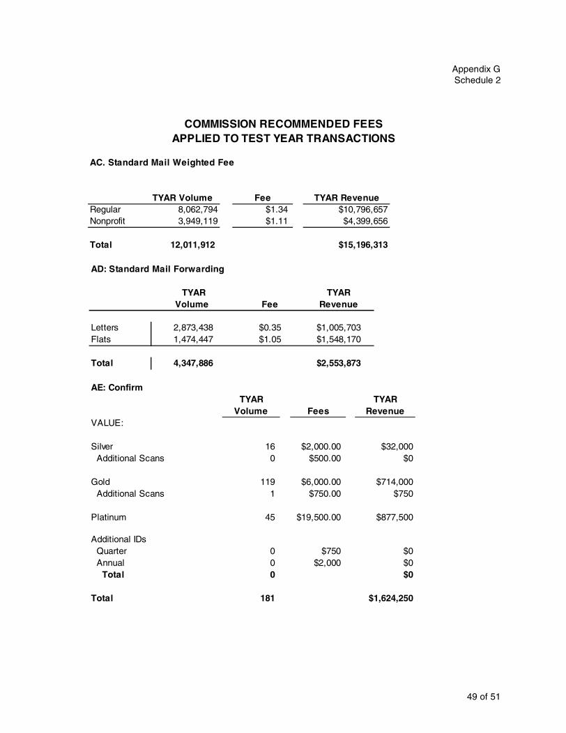
Appendix GSchedule 2
AC. Standard Mail Weighted Fee
TYAR Volume Fee TYAR RevenueRegular 8,062,794 $1.34 $10,796,657Nonprofit 3,949,119 $1.11 $4,399,656
Total 12,011,912 $15,196,313
COMMISSION RECOMMENDED FEESAPPLIED TO TEST YEAR TRANSACTIONS
AD: Standard Mail Forwarding
TYAR TYARVolume Fee Revenue
Letters 2,873,438 $0.35 $1,005,703Flats 1,474,447 $1.05 $1,548,170
Total 4,347,886 $2,553,873
AE: ConfirmTYAR TYAR
Volume Fees RevenueVALUE:
Silver 16 $2,000.00 $32,000 Additional Scans 0 $500.00 $0
Gold 119 $6,000.00 $714,000 Additional Scans 1 $750.00 $750
Platinum 45 $19,500.00 $877,500
Additional IDs Quarter 0 $750 $0 Annual 0 $2,000 $0 Total 0 $0
Total 181 $1,624,250
49 of 51

Docket N
o. R2006-1
Schedule
3, Table
1
50 of 51
R2006-1
1 R77-1 R76-1 R74-1 R71-1
24.0 52.0 69.0 85.0
24.0 63.0 87.0 96.049.0 104.0 129.0 173.0
66.0 121.0 132.0 213.0422.0 -- -- -- 137.0 -- -- --
-- -- 1.0 -- 0.0 19.0 17.0 29.0-- -- -- -- -- -- -- -- -- -- -- --
33.0 49.0 82.0 162.0
4.0 4.0 4.0 75.020.0 55.0 82.0 104.0
-- -- -- -- -- -- -- -- -- -- -- -- -- -- -- -- -- -- -- --
3.0 21.0 41.0 56.025.0 63.0 90.0 169.02.0 35.0 38.0 54.0-- -- 1.0 -- -- -- -- --
116.0 206.0 229.0 212.0-- -- -- --
29.0 57.0 62.0 103.018.0 2.0 8.0 75.0
Comparison of Markups
PRCRecommended R2000-1
Rates R2005-1 R2001-1 Modif ied R2000-1 R97-1 R94-1 R90-1 R87-1 R84-1 R80-
All Mail & Special Services 79.3 77.0 64.8 58.5 58.7 55.3 56.8 50.0 48.0 52.0 27.0
First-Class MailLetters 111.6 111.3 92.0 78.1 78.8 72.4 74.5 61.7 58.0 59.0 25.0Cards 55.4 53.0 42.6 36.8 33.0 50.5 36.7 45.9 64.0 93.0 33.0
Priority Mail 49.8 40.1 59.5 61.4 61.9 66.1 97.2 85.4 76.0 104.0 58.0Express Mail 70.4 71.8 84.0 51.3 51.3 13.6 18.9 28.6 69.0 139.0 123.0Mailgrams -- 148.8 42.4 29.4 33.3 725.5 1.6 2.8 11.0 81.0 193.0
PeriodicalsWithin County 0.1 1.4 0.2 0.4 0.3 0.5 2.7 1.5 5.0 1.0 --
Regular Rate -- -- -- 1.0 0.9 1.0 16.3 23.2 25.0 24.0 21.0Nonprofit 1/ -- -- -- (3.5) (3.9) 0.7 4.1 1.1 5.0 3.0 -- Classroom -- -- -- 2.5 1.7 (16.3) 6.8 -- 5.0 -- --
Outside County 0.2 2.9 1.3 0.3 0.1 0.8 13.8 -- -- -- --
Controlled Circulation -- -- -- -- -- -- -- -- -- --
Standard MailSingle Piece -- -- -- -- -- 4.5 20.1 26.0 15.0 --
Regular -- -- -- 37.0 37.4 34.6 23.4 47.0 41.0 46.0 34.0Nonprofit -- -- -- 8.2 7.4 13.7 1.7 0.9 8.0 (1.0) --
Regular and Nonprofit 70.8 51.5 35.1 31.9 32.1 31.2 19.0 -- -- -- -- Enhanced Carrier Route (ECR) -- -- -- 99.0 99.4 103.0 109.4 -- -- -- -- Nonprofit ECR -- -- -- 36.6 36.1 43.0 53.8 -- -- -- --
ECR and NECR 106.3 137.8 101.0 94.6 94.9 99.4 105.2 -- -- -- --
Package ServicesParcel Post 13.9 15.8 14.1 15.5 14.9 8.0 7.4 11.5 12.0 16.0 6.0Bound Printed Matter 19.4 21.8 24.1 13.1 13.9 35.6 36.6 44.5 49.0 74.0 39.0
Media Mail -- -- -- 2.4 1.9 5.6 4.6 4.8 6.0 12.0 6.0Library Rate -- -- -- (4.1) (4.5) (17.9) 0.8 0.0 1.0 2.0 --
Media and Library 3.7 0.2 9.6 1.5 1.0 1.8 4.1 -- -- -- --
Government Mail 2/ -- -- -- -- -- -- -- 120.0 136.0 132.0Free-for-the-Blind Mail -- -- -- -- -- -- -- -- -- -- International Mail 24.9 21.9 12.2 4.9 6.3 25.3 21.8 48.1 23.0 48.0 16.0Special Services 57.8 63.3 66.0 68.5 63.1 43.5 34.7 28.2 9.0 30.0 21.0
1/ Nonpro fit and Classroom were combined in R90-1.2/ Since R90-1, Government M ail has been distributed to all classes.

51 of 51
App
endix GR
unning H
/F 5
-1 R77-1 R76-1 R74-1 R71-1
0 1.000 1.000 1.000 1.000
6 1.000 1.210 1.260 1.1302 2.040 2.000 1.870 2.040
8 2.750 2.330 1.910 2.5106 17.580 -- -- -- 2 5.710 -- -- --
-- -- 0.010 -- 8 0.000 0.370 0.250 0.340
-- -- -- -- -- -- -- -- -- -- -- --
1.380 0.940 1.190 1.480
0.170 0.080 0.060 0.8809 0.830 1.060 1.190 1.220
-- -- -- -- -- -- -- -- -- -- -- -- -- -- -- -- -- -- -- --
2 0.130 0.400 0.590 0.6604 1.040 1.210 1.300 1.9902 0.080 0.670 0.550 0.640
-- -- 0.010 -- -- -- -- --
9 4.830 3.960 3.320 2.490-- -- -- --
3 1.210 1.100 0.900 1.2108 0.750 0.040 0.120 0.880
Comparison of Markup Indices
R2006-1PRC
Recommended R2000-1Rates R2005-1 R2001-1 Modified R2000-1 R97-1 R94-1 R90-1 R87-1 R84-1 R80
All Mail & Special Services 1.000 1.000 1.000 1.000 1.000 1.000 1.000 1.000 1.000 1.000 1.00
First-Class MailLetters 1.407 1.446 1.420 1.334 1.342 1.308 1.311 1.235 1.200 1.135 0.92Cards 0.698 0.688 0.658 0.629 0.561 0.913 0.645 0.919 1.330 1.788 1.22
Priority Mail 0.628 0.521 0.919 1.050 1.053 1.195 1.710 1.708 1.580 2.000 2.14Express Mail 0.888 0.933 1.296 0.878 0.873 0.245 0.332 0.572 1.420 2.673 4.55Mailgrams -- 1.934 0.654 0.502 0.568 13.114 0.028 0.056 0.230 1.558 10.85
PeriodicalsWithin County 0.001 0.018 0.004 0.006 0.005 0.010 0.048 0.031 0.110 0.019 --
Regular Rate -- -- -- 0.017 0.015 0.017 0.286 0.465 0.510 0.462 0.77Nonprof it 1/ -- -- -- (0.060) (0.066) 0.012 0.071 0.022 0.100 0.058 -- Classroom -- -- -- 0.042 0.029 (0.294) 0.119 -- 0.100 -- --
Outside County 0.002 0.037 0.021 0.005 0.002 0.015 0.242 -- -- -- --
Controlled Circulation -- -- -- -- -- -- -- -- -- --
Standard MailSingle Piece -- -- -- -- -- 0.079 0.402 0.540 0.288 --
Regular -- -- -- 0.633 0.637 0.626 0.412 0.941 0.840 0.885 1.25Nonprof it -- -- -- 0.140 0.126 0.248 0.030 0.018 0.170 (0.019) --
Regular and Nonprof it 0.892 0.670 0.542 0.546 0.547 0.563 0.335 -- -- -- -- Enhanced Carrier Route (ECR) -- -- -- 1.693 1.692 1.862 1.926 -- -- -- -- Nonprof it ECR -- -- -- 0.626 0.615 0.778 0.948 -- -- -- --
ECR and NECR 1.339 1.790 1.560 1.617 1.616 1.797 1.851 -- -- -- --
Package ServicesParcel Post 0.175 0.206 0.218 0.264 0.253 0.144 0.131 0.230 0.240 0.308 0.22Bound Printed Matter 0.244 0.283 0.373 0.224 0.237 0.643 0.644 0.890 1.020 1.423 1.44
Media Mail -- -- -- 0.040 0.032 0.101 0.080 0.097 0.110 0.231 0.22Library Rate -- -- -- (0.070) (0.076) (0.324) 0.013 0.001 0.030 0.038 --
Media and Library 0.046 0.002 0.148 0.025 0.017 0.033 0.073 -- -- -- --
Government Mail 2/ -- -- -- -- -- -- -- 2.480 2.615 4.88Free-for-the-Blind Mail -- -- -- -- -- -- -- -- -- -- International Mail 0.314 0.285 0.188 0.084 0.106 0.457 0.383 0.962 0.480 0.923 0.59Special Services 0.728 0.823 1.019 1.171 1.074 0.787 0.611 0.564 0.200 0.577 0.77
1/ Nonprof it and Classroom w ere combined in R90-1.2/ Since R90-1, Government Mail has been distributed to all classes.


Appendix H
COMPARISON OF ESTIMATED TEST YEAR VOLUMES1
USPS Est. PRC Est.TYAR Volume TYAR Volume
First-Class MailSingle-Piece Letters 37,206,438 37,613,747
Presort Letters 929,256 1,159,748Automation Letters 47,497,945 46,406,152
Workshared Letters 48,427,200 47,565,900Total Letters 85,633,639 85,179,646
Single-Piece Cards 2,358,960 2,391,827Presort Cards 300,783 277,854Automation Cards 2,997,708 3,068,354
Workshared Cards 3,298,491 3,346,208Total Cards 5,657,451 5,738,035
Total First-Class 91,291,090 90,917,681
Priority Mail 829,079 829,856Express Mail 42,683 42,683
PeriodicalsWithin County 700,140 705,280Regular Rate 6,290,945 6,287,446Nonprofit 1,698,941 1,697,440Classroom 60,068 60,230
Total Periodicals 8,750,094 8,750,396
Standard MailRegular Presort 2,859,038 3,011,563Regular Automation 60,067,212 60,577,976
Total Regular 62,926,250 63,589,539Nonprofit Presort 1,129,174 936,648Nonprofit Automation 11,243,381 11,479,416
Total Nonprofit 12,372,554 12,416,064Total Regular and Nonprofit 75,298,805 76,005,603
ECR 29,346,811 29,682,108Nonprofit ECR 2,522,847 2,529,325
Total ECR and NECR 31,869,658 32,211,433Total Standard Mail 107,168,463 108,217,035
(Pieces in Thousands)
1 of 2
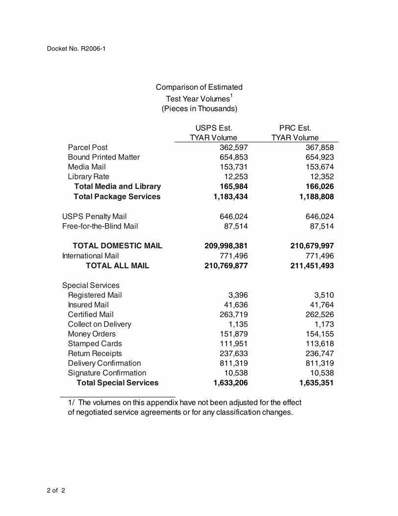
Docket No. R2006-1
USPS Est. PRC Est.TYAR Volume TYAR Volume
Parcel Post 362,597 367,858Bound Printed Matter 654,853 654,923Media Mail 153,731 153,674Library Rate 12,253 12,352
Total Media and Library 165,984 166,026Total Package Services 1,183,434 1,188,808
USPS Penalty Mail 646,024 646,024Free-for-the-Blind Mail 87,514 87,514
TOTAL DOMESTIC MAIL 209,998,381 210,679,997International Mail 771,496 771,496
TOTAL ALL MAIL 210,769,877 211,451,493
Special ServicesRegistered Mail 3,396 3,510Insured Mail 41,636 41,764Certified Mail 263,719 262,526Collect on Delivery 1,135 1,173Money Orders 151,879 154,155Stamped Cards 111,951 113,618Return Receipts 237,633 236,747Delivery Confirmation 811,319 811,319Signature Confirmation 10,538 10,538
Total Special Services 1,633,206 1,635,351
1/ The volumes on this appendix have not been adjusted for the effect of negotiated service agreements or for any classification changes.
Comparison of Estimated
Test Year Volumes1
(Pieces in Thousands)
2 of 2

Appendix I
ECONOMIC DEMAND MODELS AND FORECAST METHODOLOGY
[1] For this proceeding, and for all general rate proceedings since Docket No.
R80-1, the Commission has adopted the econometric demand models and forecasting
methods developed by Postal Service witnesses. In the present case, these models and
methods are described in detail for all categories of domestic mail and special services in
the testimony of witness Thress. The models are similar in design to those provided by
witness Thress, and used by the Commission, in Docket Nos. R97-1, R2000-1, R2001-1
and R2005-1. They are somewhat similar to earlier models supplied by Postal Service
witnesses Tolley and Musgrave. Witness Thress’ demand models and forecasts are
described extensively in his direct testimony (USPS-T-7). The data, econometrics and
forecasting process are found in four supporting library references: USPS-LR-L-63,
USPS-LR-L-64, USPS-LR-L-65, and USPS-LR-L-66. Additional original econometric
evidence is also contained in witness Thress’ rebuttal testimony (USPS-RT-2).
[2] Postal Service witness Bernstein discusses aspects of the demand models
relating to the effects of electronic diversion via the Internet. See USPS-T-8. Forecasts
of volumes and revenues for International mail and services are found in the Postal
Service response to Presiding Officer’s Information Request No. 1, Question 11 and in
the supporting library reference USPS-LR-L-121.
[3] The Postal Service models were criticized in the testimony of witnesses
Clifton and Kelejian, sponsored by the Greeting Card Association (GCA). Witness
Clifton asserts that the equation used by witness Thress to model the demand for
First-Class single-piece mail fails to correctly represent the impact of electronic diversion
on the price elasticity of this large and disparate subclass. He argues that the price
elasticity estimated by witness Thress has too small a magnitude and offers substitute
equations for First-Class single-piece and Standard Regular mail.
[4] Witness Kelejian raises several problematic technical aspects of witness
Thress’ econometric practice. His comments and criticisms apply to many of the
equations fit by witness Thress and suggest general questions regarding the statistical

Docket No. R2006-1
qualities of the Postal Service demand model and, in particular, the estimates of price
elasticities. Witness Kelejian’s critique of the Postal Service models and econometrics
was submitted, at first, as an attachment to the Clifton testimony and later as direct
testimony in GCA-T-5.
[5] Witnesses Thress, Clifton and Kelejian have also responded extensively to
written interrogatories, and, orally, in hearings.
[6] In response to this testimony, the Commission has conducted a review of the
Postal Service econometric demand models and forecast methodology. The purpose of
this review is two-fold. First, it was necessary for the Commission to evaluate issues
raised by GCA witnesses to determine if the Postal Service econometric models are
seriously flawed. This evaluation led to an investigation focused more widely on the
reliability of the forecasts and elasticity estimates used by the Commission, on the
econometric practice of witness Thress, on his demand equations and on potential
opportunities to replace or improve them for future proceedings. Commission findings, in
summary, are as follows:
• Volume forecasts made with the Postal Service models appear to be unbiased and highly accurate in the aggregate. The accuracy is also excellent for the larger subclasses. However, the reliability of these forecasts declines precipitously for smaller subclasses and when the mailstream is divided into worksharing categories.
• The conventional statistical properties of witness Thress’ long-run own-price elasticity estimates are fair-to-good, but the estimates are not often robust.
• The lag structures for price effects found in witness Thress’ equations are mostly assumed or the forced result of his estimation method.
• Witness Thress’ reported own-price elasticities do not conform to the conventional economic definition of price elasticity when discounts are included among the explanatory variables of his equations. On those occasions, the conventional definition implies that the price elasticities have higher absolute values.
• Witness Thress’ econometric practice is mostly conventional. The technical issues raised by witness Kelejian would not have much effect on the volume forecasts and are likely to have only a minor impact on the estimates of price elasticities.
• It is impossible to tell from the available evidence whether witness Thress has underestimated the price elasticity for First-Class single-piece mail.
2 of 36

Appendix I
• Witness Clifton’s equations for First-Class single-piece and Standard Regular mail are not preferable to those of witness Thress.
• The demand equations specified by witness Thress are complex, frequently non-linear and commonly include explanatory variables that exhibit a high degree of co-linearity. There appear to be many ways that the Postal Service models could be simplified and improved.
• The Postal Service forecasting methodology is well-suited to the Commission’s needs and to the Postal Service models. However, there are several ways that the Commission could potentially improve the forecasts for a rate proceeding by updating the information from which they are derived.
1. How reliable are the forecasts of volumes produced by the Postal Service forecasting models?
[7] The Commission’s recommended rates are designed to meet a revenue
target that allows Postal Service to cover the total cost of providing mail and related
services plus other permitted expenses during the test year. If determining these rates is
to be more than an academic exercise, then the volume forecasts used by the
Commission must be forecasts of the actual volumes of mail and special services that
are expected to arise in response to the recommended rates during the test year. The
more accurate the volume forecasts, the more accurate will be the corresponding
forecast of postal revenue.
[8] An inaccurate forecast will affect the Commission’s projection of net revenue
during the test year because the recommended rates exceed marginal costs for virtually
every category of domestic mail and service. If demand is underestimated, this creates
an unintended net surplus in the test year. Conversely, an overestimate creates a net
deficit. Therefore, the quality of the volume forecasts largely determines the confidence
the Commission can place in its judgment that the recommended rates will meet the
prescribed revenue target.
[9] The volume forecasts may be inaccurate for many reasons, some of which
have little to do with the quality of the Postal Service demand models or witness Thress’
3 of 36

Docket No. R2006-1
econometrics. Any listing of factors affecting the accuracy of the forecasts ought to
include the following:
• Sampling error: volume statistics periodically reported by the Postal Service in the Revenue, Pieces, and Weights (RPW) reports are derived from samples of only a very small portion of the mailstream. The sampling errors left in the volume statistics are inherently random and can not be reduced by perfecting the demand models or the econometrics.
• Sample size: the samples that are available for fitting the Postal Service models are fairly short quarterly time series, typically of about 80 observations. This limits the complexity of the models primarily because the number of estimated parameters must be small relative to the size of the sample.
• Autoregressive disturbances: the errors from equations fit to a time series often exhibit nonrandom patterns over time. This characteristic tends to reduce the useful information contained in a sample.
• Colinearity: many variables that describe economic activity, and especially postal rates, are highly correlated over time making it difficult to statistically distinguish between their effects within a small sample.
• Structural change: variations in postal volumes are partly caused by structural changes in postal markets occurring within the time period spanned by the samples. This often means that the explanatory variables describing the changes have incomplete records.
• Forecasts off a base year: the Postal Service methodology is to forecast off a recent base year. This embeds the average of the forecast errors in the base year within the test year forecasts.
• Forecasts of economic activity and non-postal prices: the Postal Service demand models make volumes a function of an array of variables representing economic activity and non-postal price levels. The accuracy of the volume forecasts depends in turn on the accuracy of projections into the future of these explanatory variables.
• Installation of the tariff: the Postal Service does not always enact a new tariff exactly as recommended by the Commission. Often, different parts of a recommended tariff are installed on dates that differ from the date of installation assumed for the volume forecasts.
[10] Sample size, autoregressive disturbances, colinearity, and structural change
all place practical limits on the complexity of the equations that can be successfully fit to
the available data. Therefore, of necessity, any econometric model will be an
approximation. Sampling error, forecasting off a base year and the use of imperfect
forecasts of economic activity and non-postal prices would cause errors in the forecasts
4 of 36

Appendix I
of volumes even in the unlikely event that the econometrics had yielded precise
estimates of the “true” demand equations.
[11] The Commission’s assessments of the reliability of the volume forecasts are
based on evidence from several sources. First, coefficients of variation (CVs) for the
GFY 2004 and GFY 2005 RPW reports can be found attached to the testimony of Postal
Service witness Pafford in Docket No. R2005-1 (USPS-T-4) and Docket No. R2006-1
(USPS-T-3). The CV of a statistic is the ratio of the statistic’s standard deviation to its
mean value and is usually expressed as a percentage. The CVs for the RPW statistics
are measurements of the magnitudes of the sampling errors in the annual RPW
summary reports.
[12] A second important source of evidence is the goodness-of-fit statistics for
the fitted equations of the Postal Service models. These statistics are found, for the
current proceeding, throughout the direct testimony of witness Thress. For each of the
subclass demand equations, witness Thress reports the mean square error (MSE) and
the adjusted R-Squared. He also fits share equations to predict the division of several
worksharing categories into automated and non-automated shares. For the share
equations he reports the mean absolute percentage error (MAPE).
[13] Third, witness Thress has provided econometric models and forecasts for
the most recent past four general rate proceedings as well as the present one. The
models used in these past cases are sufficiently similar in design and estimation to the
current edition that the performance of the forecasts versus the actual volumes should
provide a “track record” to reveal the reliability of the forecasts made for this proceeding.
And, fourth, the Commission’s rules require the Postal Service to provide before-rates
forecasts of volumes for the quarters that intervene between the base year (GFY 2005)
and the test year (GFY 2008). [Rules of Practice and Procedure 3001.54(j)] Most of
these forecasts can be found attached to witness Thress direct testimony See
USPS-T-7, Attachment A. Forecasts for International Mail are contained in the response
to Presiding Officer’s Information Request No. 1, Question 11. USPS-LR-L-121. The
before-rates quarterly forecasts for GFY 2006 can now be directly compared to the
5 of 36

Docket No. R2006-1
quarterly GFY 2006 volumes which were provided by the Postal Service in the
end-of-year GFY 2006 RPW report received by the Commission in December 2006.
[14] Some of this evidence is displayed in the RPW format in Tables 1 and 2.
The RPW CVs are those for GFY 2005. The subclass CVs are derived from witness
Thress’ MSEs using the formula: . The
share CVs are the MAPEs for the share equations. The CVs for classes and other
combinations of categories were computed by assuming that the component errors are
uncorrelated. All of the CVs are expressed as percentages. Table 1 displays the
percentage errors in the forecasts for the past four rate proceedings. These percentage
errors are derived as percentages of the forecasts: (Actual test year volume - Forecast
test year volume) / (Forecast test year volume). See Docket No. R97-1, R2000-1,
R201-1, and R2005-1 Opinion and Recommended Decision. The actual volumes are
those from the RPW for the test year. Table 2 displays the percentage errors of the
before-rates forecasts made by witness Thress for the four quarters of GFY 2006. The
formula for these percentage errors is: (Actual quarterly volume – Forecast quarterly
volume) / (Forecast quarterly volume). Both tables show the percentage errors in
witness Thress’ before-rates forecasts for all of GFY 2006.
[15] The Commission believes that the testimony and statistics referenced above
support the Commission’s reliance on aggregate forecasts of test year volumes and
revenues made with the Postal Service models and forecasting methodology. The very
low RPW and subclass CVs for total domestic mail and for the four major mail classes
show that the quality of the RPW data is high at this level and that the models should
produce forecasts with low percentage errors. This predicted reliability is borne out in
the actual performance of the forecasts in prior rate proceedings and during GFY 2006.
The forecast errors are no more than a few percentage points in all years and quarters
except GFY 2003, the test year for the forecasts from Docket No. R2001-1. Postal
volumes were still depressed in GFY 2003 due to the 9/11 and Anthrax attacks.
CV MSE{ }exp MSE–{ }exp–2
--------------------------------------------------------------------=
6 of 36

Appendix I
Table I-1
Camparisons of Percentage Errors - Postal Rate Proceedings Forecast versus RPW Numbers of Pieces
Percentage Difference Actual vs ForecastRPW Volumes RPW
CVSubclass
CVShare
CVR97-1 R2000-1 R2001-1 R2005-1 GFY 2006
First Class MailSingle-Piece Letters 0.28% 1.57% 0.11% -1.24% -0.60% -0.92% 1.59%Nonautomation Presort Letters 1.96% 1.09% 5.08% -8.44% 77.24% -17.14% 54.97% 15.33%Automation Presort Letters 0.17% 1.09% 0.35% -2.14% -8.82% -7.23% 2.90% 1.87%
Total Letters 0.14% 0.94% -1.21% -2.69% -4.43% 1.75% 1.96%Single-Piece Cards 1.14% 3.86% -5.46% -4.10% -2.82% -7.30% -7.75%Nonautom. Presort Cards 10.48% 3.21% 8.92% -16.08% 68.95% 78.02% 25.18% 10.95%Automation Presort Cards 2.54% 3.21% 1.76% 3.94% -13.18% -6.12% 12.32% 6.65%
Total Cards 1.47% 2.47% -3.56% -2.64% -1.02% 4.10% 0.55%Total First-Class 0.13% 0.89% -1.34% -2.69% -4.26% 1.89% 1.88%
Priority Mail 0.72% 2.25% 5.18% -2.23% -27.03% 15.63% 2.55%Express Mail 1.67% 10.37% -3.35% -20.14% 11.04% 2.82%Mailgrams 22.57% -10.10% 2.78% 2.42%Periodicals
Within County 2.29% 6.25% 1.63% 2.51% -7.03% 1.37% 0.48%Regular Rate 0.07% 2.17% 0.11% -3.04% -8.34% -0.45% -1.28%Nonprofit 0.31% 5.87% -0.36% 2.99% 0.38% 0.26% 2.15%Classroom 0.30% 5.87% 33.81% 14.29% 4.04% -11.00% -8.15%
Total Periodicals 0.20% 2.02% 0.30% -1.28% -6.46% -0.24% -0.51%Standard Mail
Single-Piece -8.35%Regular - Non-automation Presort 1.03% 1.58% 2.69% -29.34% 19.34% -10.10% 1.24% -4.34%Regular - Automation Presort 0.13% 1.58% 0.17% -0.71% 1.39% -0.55% -3.13% -2.62%Enhanced Carrier Route 0.37% 2.07% 17.70% -1.11% -11.46% 2.51% 1.21%
Total Standard Regular 0.05% 1.26% 3.01% 1.50% -5.53% -0.94% -1.27%Nonprofit - Non-automation Presort 1.02% 1.69% 2.00% 3.51% -11.68% 1.47% -1.06% 1.98%Nonprofit - Automation Presort 0.34% 1.69% 0.43% -1.79% 2.59% -3.79% -3.14% -0.01%Nonprofit Enhanced Carrier Route 2.09% 7.13% 2.24% 1.52% -7.98% -15.24% -4.93%
Total Standard Nonprofit 0.21% 1.97% 0.45% -0.93% -3.91% -5.35% -0.72% Total Standard Mail 0.06% 1.11% 2.57% 1.10% -5.28% -1.59% -1.19%
Package ServicesParcel Post 0.26% 3.75% 49.21% -12.11% 4.26% 7.81% -8.26%Bound Printed Matter 0.08% 7.26% -12.34% 2.70% -7.43% -1.31% 1.59%Media Mail 0.58% 6.85% -7.81% 6.51% 12.95% -3.32% 2.17%Library Rate 1.72% 6.85% -7.48% -1.31% -34.99% -3.68% 12.64%
Total Package Services 0.16% 4.01% 1.76% -1.54% -1.47% 0.98% -1.47%USPS Penalty Mail 2.03% 11.76% 26.61% 2.73% 10.72% 52.42% 62.64%Free-for-the-Blind 3.44% 27.19% -6.40% -17.81% 50.20% -1.03% -6.60%
Total Domestic Mail 0.68% 0.46% -0.99% -4.90% 0.29% 0.43%International Mail -6.39% 3.84% -33.21% -6.31% -3.64%
Total All Mail 0.42% -0.97% -5.06% 0.27% 0.41%Special Services
Registry - Fees Affixed 1.88% 7.44% 0.69% 39.09% -0.21% 136.11% 100.76%Insurance 4.31% 7.37% 34.42% 26.22% -6.84% 44.59% 3.59%Collect On Delivery 1.60% 9.82% 0.82% 13.37% -40.10% -9.32% 6.76%Certified 1.31% 7.65% -7.52% -3.87% -10.40% -4.69% 0.97%Return Receipts & Confirmations 0.34% 8.50% 56.85% 41.13% 8.09% 1.40%Money Orders 2.00% -13.97% -3.62% -13.15% -2.07% 0.31%
Total Domestic Services 5.76% -7.77% 14.45% 12.75% 5.23% 1.24%
7 of 36

Docket No. R2006-1
Table I-2
Camparisons of Percentage Errors - Before Rates Forecasts Forecast versus RPW Numbers of Pieces
Percentage Difference Actual vs ForecastRPW Volumes RPW
CVSubclass
CVShare
CV2006 Q1 2006 Q2 2006 Q3 2006 Q4 GFY 2006
First Class MailSingle-Piece Letters 0.28% 1.57% -2.05% 5.97% 2.45% 0.56% 1.59%Nonautomation Presort Letters 1.96% 1.09% 5.08% 6.40% 10.23% 22.59% 25.69% 15.33%Automation Presort Letters 0.17% 1.09% 0.35% 0.35% 2.95% 2.57% 1.59% 1.87%
Total Letters 0.14% 0.94% -0.72% 4.43% 2.83% 1.50% 1.96%Single-Piece Cards 1.14% 3.86% -8.90% -5.82% -6.26% -9.99% -7.75%Nonautom. Presort Cards 10.48% 3.21% 8.92% -16.12% 18.10% -1.15% 47.65% 10.95%Automation Presort Cards 2.54% 3.21% 1.76% -1.73% 8.14% 10.06% 10.95% 6.65%
Total Cards 1.47% 2.47% -5.68% 2.57% 2.20% 3.57% 0.55%Total First-Class 0.13% 0.89% -1.00% 4.32% 2.79% 1.62% 1.88%
Priority Mail 0.72% 2.25% -2.93% 9.20% 1.23% 3.65% 2.55%Express Mail 1.67% 1.88% 3.35% 3.73% 2.29% 2.82%Mailgrams 22.57%Periodicals
Within County 2.29% 6.25% -0.83% -2.95% 2.53% 3.18% 0.48%Regular Rate 0.07% 2.17% -2.33% -0.36% -1.02% -1.44% -1.28%Nonprofit 0.31% 5.87% 5.82% 1.14% -1.62% 3.31% 2.15%Classroom 0.30% 5.87% -21.38% 8.37% -18.92% -0.35% -8.15%
Total Periodicals 0.20% 2.02% -0.72% -0.20% -0.97% -0.13% -0.51%Standard Mail
Single-PieceRegular - Non-automation Presort 1.03% 1.58% 2.69% -2.47% -3.05% -4.66% -7.35% -4.34%Regular - Automation Presort 0.13% 1.58% 0.17% -2.00% -2.24% -4.25% -1.98% -2.62%Enhanced Carrier Route 0.37% 2.07% -1.21% 1.45% 4.99% 0.11% 1.21%
Total Standard Regular 0.05% 1.26% -1.71% -0.96% -0.99% -1.39% -1.27%Nonprofit - Non-automation Presort 1.02% 1.69% 2.00% 0.57% 2.27% 3.77% 1.63% 1.98%Nonprofit - Automation Presort 0.34% 1.69% 0.43% 1.99% 1.06% -2.75% -0.74% -0.01%Nonprofit Enhanced Carrier Route 2.09% 7.13% 1.16% -4.39% -8.14% -8.72% -4.93%
Total Standard Nonprofit 0.21% 1.97% 1.68% 0.20% -3.04% -2.10% -0.72% Total Standard Mail 0.06% 1.11% -1.21% -0.79% -1.27% -1.49% -1.19%
Package ServicesParcel Post 0.26% 3.75% -11.19% -1.87% -10.49% -8.27% -8.26%Bound Printed Matter 0.08% 7.26% 1.32% 6.53% 2.32% -2.90% 1.59%Media Mail 0.58% 6.85% -0.24% 6.09% -5.67% 9.23% 2.17%Library Rate 1.72% 6.85% -8.20% 38.10% 11.96% 11.32% 12.64%
Total Package Services 0.16% 4.01% -3.95% 4.16% -3.05% -2.63% -1.47%USPS Penalty Mail 2.03% 11.76% 31.02% 54.80% 131.16% 28.53% 61.64%Free-for-the-Blind 3.44% 27.19% 6.06% -1.56% -14.53% -15.86% -6.60%
Total Domestic Mail 0.68% -1.02% 1.82% 1.00% 0.04% 0.43%International Mail 1.30% -6.52% -4.11% -6.15% -3.64%
Total All Mail -1.01% 1.79% 0.98% 0.02% 0.41%Special Services
Registry - Fees Affixed 1.88% 7.44% 97.98% 109.14% 97.25% 98.61% 100.76%Insurance 4.31% 7.37% 4.24% 2.91% -1.90% 9.54% 3.59%Collect On Delivery 1.60% 9.82% -12.57% 11.04% -0.28% 29.12% 6.76%Certified 1.31% 7.65% -4.83% 8.25% -3.57% 4.09% 0.97%Return Receipts & Confirmations 0.34% 8.50% 1.83% 3.21% -5.58% 6.51% 1.40%Money Orders 2.00% -0.24% 1.59% -0.43% 0.27% 0.31%
Total Domestic Services 5.76% 0.54% 3.91% -4.49% 5.39% 1.24%
8 of 36

Appendix I
[16] The Postal Service model also seems likely to produce reliable test year
forecasts for all of the larger subclasses of mail, e.g., First-Class single-piece letters,
First-Class presort letters, Regular rate Periodicals, Standard Regular presort, Standard
ECR, and Standard Nonprofit presort. Again, the low CVs show, first, that the RPW data
are fairly accurate and, second, that the Postal Service models are close fits. This
pattern is mostly, but not always, confirmed by the patterns of percentage forecast errors
from past rate proceedings and during GFY 2006.
[17] The forecasting reliability of the Postal Service models and methodology
deteriorates rapidly as the subclasses become smaller in volume as measured by the
number of pieces. The CVs in Tables 1 and 2 suggest that this decline can not be
entirely attributed to the rise in sampling error. There are a number of mid-sized
subclasses, such as Bound Printed Matter, with small RPW CVs, but large subclass
CVs. This indicates that the Postal Service model, and not the sampling error in the
RPW data, is responsible for the increasing unreliability of the forecasts.
[18] The forecasts that depend upon witness Thress’ share models are the least
reliable of the volume forecasts. The fairly high CVs for the share models show that they
are major contributors to inaccuracies in the volume forecasts wherever they are applied
to divide a subclass of mail into automated and non-automated components. Many of
the share models consist of simply extrapolating base year worksharing percentages.
[19] Forecasts for domestic special services are less reliable, even in the
aggregate, than the volume forecasts for the major mail classes. This should not be
surprising in view of the high subclass CV (5.76 percent) that emerges from witness
Thress’ equation fits for domestic services. In past proceedings, witness Thress’
econometric models for domestic special services were also somewhat less successful
than his mail equations. For this reason, the forecast errors for all domestic services
have occasionally exceeded 10 percent.
[20] There are no apparent biases in the forecasts except for those made in
Docket No. R2001-1 for GFY 2003 which were too high in the aggregate and for most
kinds of mail. Otherwise, positive and negative percentage differences between actual
9 of 36

Docket No. R2006-1
and predicted volumes are about equally frequent in Tables 1 and 2. In Docket No.
R2001-1 the model and forecasts did not reflect the impact of the 9/11 and Anthrax
attacks on postal volumes. Postal volumes took time to recover from the effects of these
attacks and remained somewhat depressed in GFY 2003.
2. How accurate and robust are witness Thress’ estimates of price elasticities?
[21] Estimates of postal rate elasticities are necessary to correctly predict the
revenue impact of changes in postal rates. If the own-price elasticity of a postal service
is underestimated (absolutely), then revenues from the service will be overestimated
after a rate increase. The rate elasticities are also useful for making comparisons of the
value-of-use of postal services to customers. The standard economic measure of
value-of-use is consumers’ surplus. Calculations of consumers’ surplus for a proposed
set of postal rates depend almost entirely on the estimates of postal price elasticities
found in the demand models.
[22] The statistical accuracy of the estimates of the parameters of an
econometric model is commonly assessed under the assumption that the fitted equation
structurally matches the “true” equation that generated the observations in the sample.
The usual statistics for evaluating the statistical significance of coefficients and
performing more sophisticated tests presume that the equation is correct in form and that
the disturbances have certain assumed random properties. On the other hand,
robustness describes the stability of the parameter estimates when the retained
assumptions are relaxed in ways that do not conflict with the underlying economic theory.
Estimates are robust if they are little changed by alterations in the explanatory variables
not dictated by the relevant economic theory, by the mathematical form of the fitted
equation, by arbitrary divisions of the sample, and so on. The advantage to having
robust estimates is largely practical. If the estimates are robust, it is not necessary to
10 of 36
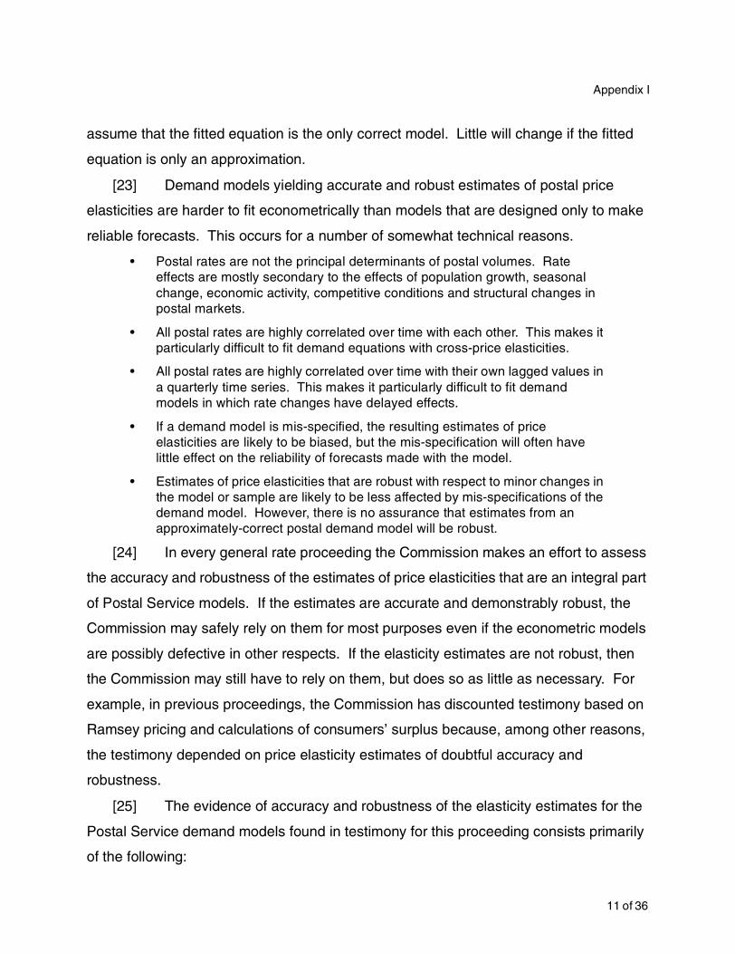
Appendix I
assume that the fitted equation is the only correct model. Little will change if the fitted
equation is only an approximation.
[23] Demand models yielding accurate and robust estimates of postal price
elasticities are harder to fit econometrically than models that are designed only to make
reliable forecasts. This occurs for a number of somewhat technical reasons.
• Postal rates are not the principal determinants of postal volumes. Rate effects are mostly secondary to the effects of population growth, seasonal change, economic activity, competitive conditions and structural changes in postal markets.
• All postal rates are highly correlated over time with each other. This makes it particularly difficult to fit demand equations with cross-price elasticities.
• All postal rates are highly correlated over time with their own lagged values in a quarterly time series. This makes it particularly difficult to fit demand models in which rate changes have delayed effects.
• If a demand model is mis-specified, the resulting estimates of price elasticities are likely to be biased, but the mis-specification will often have little effect on the reliability of forecasts made with the model.
• Estimates of price elasticities that are robust with respect to minor changes in the model or sample are likely to be less affected by mis-specifications of the demand model. However, there is no assurance that estimates from an approximately-correct postal demand model will be robust.
[24] In every general rate proceeding the Commission makes an effort to assess
the accuracy and robustness of the estimates of price elasticities that are an integral part
of Postal Service models. If the estimates are accurate and demonstrably robust, the
Commission may safely rely on them for most purposes even if the econometric models
are possibly defective in other respects. If the elasticity estimates are not robust, then
the Commission may still have to rely on them, but does so as little as necessary. For
example, in previous proceedings, the Commission has discounted testimony based on
Ramsey pricing and calculations of consumers’ surplus because, among other reasons,
the testimony depended on price elasticity estimates of doubtful accuracy and
robustness.
[25] The evidence of accuracy and robustness of the elasticity estimates for the
Postal Service demand models found in testimony for this proceeding consists primarily
of the following:
11 of 36
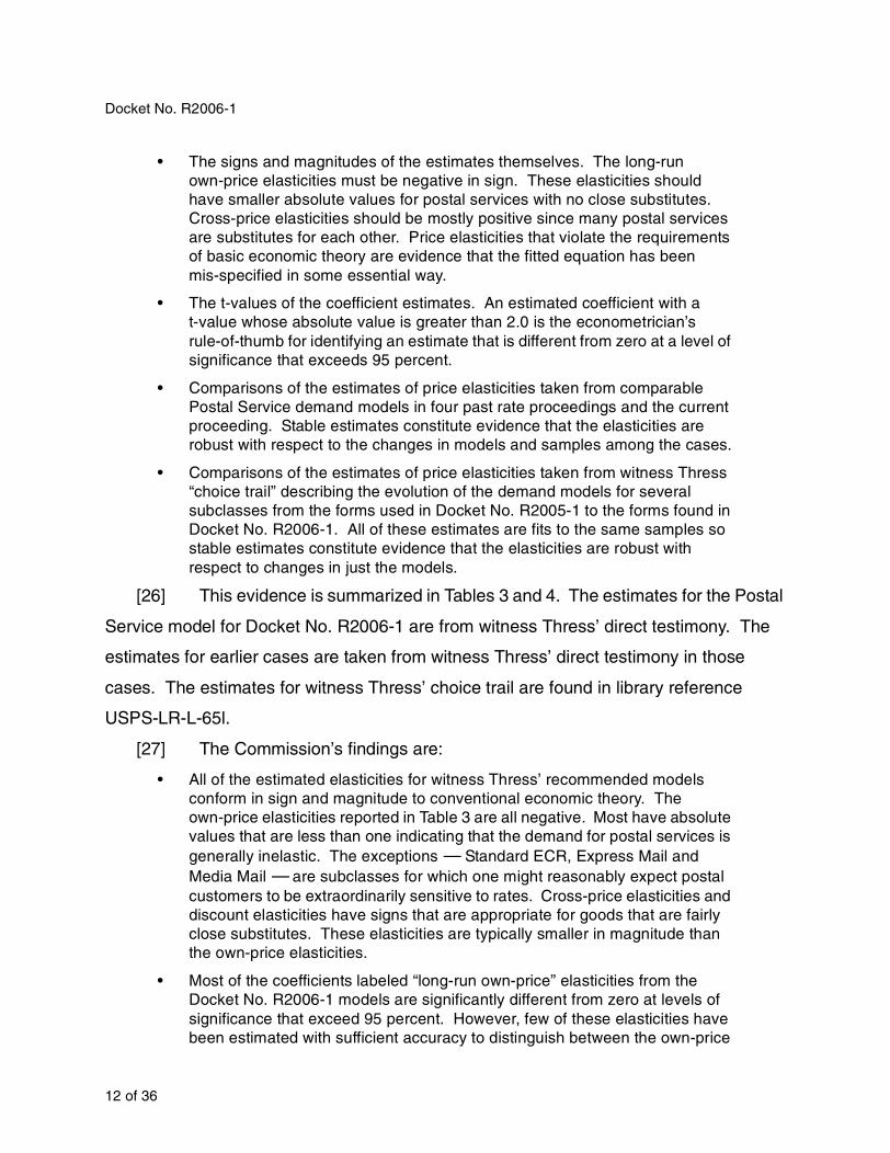
Docket No. R2006-1
• The signs and magnitudes of the estimates themselves. The long-run own-price elasticities must be negative in sign. These elasticities should have smaller absolute values for postal services with no close substitutes. Cross-price elasticities should be mostly positive since many postal services are substitutes for each other. Price elasticities that violate the requirements of basic economic theory are evidence that the fitted equation has been mis-specified in some essential way.
• The t-values of the coefficient estimates. An estimated coefficient with a t-value whose absolute value is greater than 2.0 is the econometrician’s rule-of-thumb for identifying an estimate that is different from zero at a level of significance that exceeds 95 percent.
• Comparisons of the estimates of price elasticities taken from comparable Postal Service demand models in four past rate proceedings and the current proceeding. Stable estimates constitute evidence that the elasticities are robust with respect to the changes in models and samples among the cases.
• Comparisons of the estimates of price elasticities taken from witness Thress “choice trail” describing the evolution of the demand models for several subclasses from the forms used in Docket No. R2005-1 to the forms found in Docket No. R2006-1. All of these estimates are fits to the same samples so stable estimates constitute evidence that the elasticities are robust with respect to changes in just the models.
[26] This evidence is summarized in Tables 3 and 4. The estimates for the Postal
Service model for Docket No. R2006-1 are from witness Thress’ direct testimony. The
estimates for earlier cases are taken from witness Thress’ direct testimony in those
cases. The estimates for witness Thress’ choice trail are found in library reference
USPS-LR-L-65l.
[27] The Commission’s findings are:
• All of the estimated elasticities for witness Thress’ recommended models conform in sign and magnitude to conventional economic theory. The own-price elasticities reported in Table 3 are all negative. Most have absolute values that are less than one indicating that the demand for postal services is generally inelastic. The exceptions — Standard ECR, Express Mail and Media Mail — are subclasses for which one might reasonably expect postal customers to be extraordinarily sensitive to rates. Cross-price elasticities and discount elasticities have signs that are appropriate for goods that are fairly close substitutes. These elasticities are typically smaller in magnitude than the own-price elasticities.
• Most of the coefficients labeled “long-run own-price” elasticities from the Docket No. R2006-1 models are significantly different from zero at levels of significance that exceed 95 percent. However, few of these elasticities have been estimated with sufficient accuracy to distinguish between the own-price
12 of 36
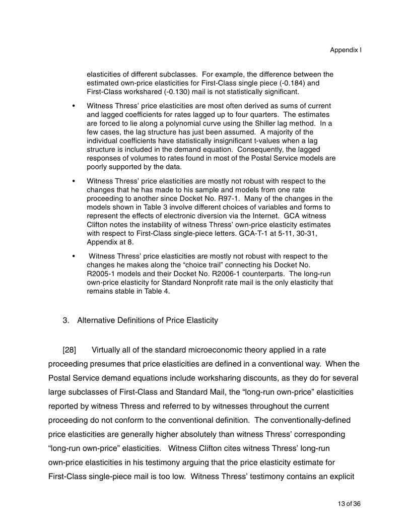
Appendix I
elasticities of different subclasses. For example, the difference between the estimated own-price elasticities for First-Class single piece (-0.184) and First-Class workshared (-0.130) mail is not statistically significant.
• Witness Thress’ price elasticities are most often derived as sums of current and lagged coefficients for rates lagged up to four quarters. The estimates are forced to lie along a polynomial curve using the Shiller lag method. In a few cases, the lag structure has just been assumed. A majority of the individual coefficients have statistically insignificant t-values when a lag structure is included in the demand equation. Consequently, the lagged responses of volumes to rates found in most of the Postal Service models are poorly supported by the data.
• Witness Thress’ price elasticities are mostly not robust with respect to the changes that he has made to his sample and models from one rate proceeding to another since Docket No. R97-1. Many of the changes in the models shown in Table 3 involve different choices of variables and forms to represent the effects of electronic diversion via the Internet. GCA witness Clifton notes the instability of witness Thress’ own-price elasticity estimates with respect to First-Class single-piece letters. GCA-T-1 at 5-11, 30-31, Appendix at 8.
• Witness Thress’ price elasticities are mostly not robust with respect to the changes he makes along the “choice trail” connecting his Docket No. R2005-1 models and their Docket No. R2006-1 counterparts. The long-run own-price elasticity for Standard Nonprofit rate mail is the only elasticity that remains stable in Table 4.
3. Alternative Definitions of Price Elasticity
[28] Virtually all of the standard microeconomic theory applied in a rate
proceeding presumes that price elasticities are defined in a conventional way. When the
Postal Service demand equations include worksharing discounts, as they do for several
large subclasses of First-Class and Standard Mail, the “long-run own-price” elasticities
reported by witness Thress and referred to by witnesses throughout the current
proceeding do not conform to the conventional definition. The conventionally-defined
price elasticities are generally higher absolutely than witness Thress’ corresponding
“long-run own-price” elasticities. Witness Clifton cites witness Thress’ long-run
own-price elasticities in his testimony arguing that the price elasticity estimate for
First-Class single-piece mail is too low. Witness Thress’ testimony contains an explicit
13 of 36
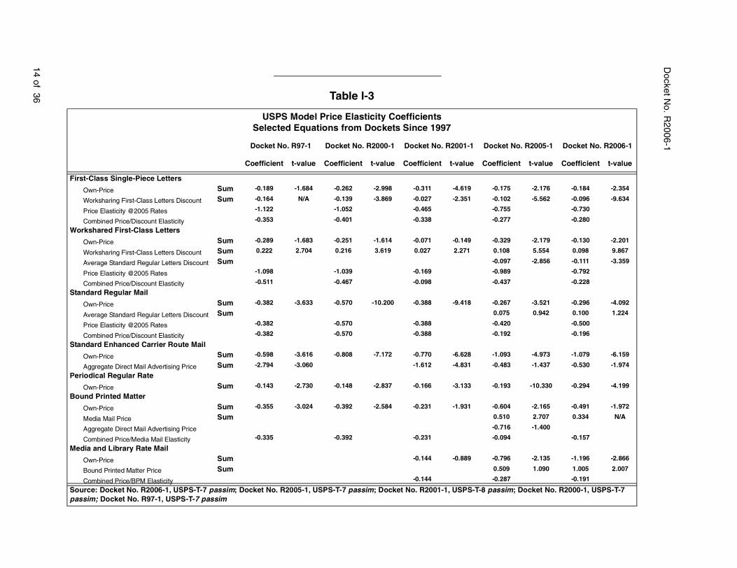
Docket N
o. R2006-1
14 of 36
. R2005-1 Docket No. R2006-1
t-value Coefficient t-value
-2.176 -0.184 -2.354
-5.562 -0.096 -9.634
-0.730
-0.280
-2.179 -0.130 -2.201
5.554 0.098 9.867
-2.856 -0.111 -3.359
-0.792
-0.228
-3.521 -0.296 -4.092
0.942 0.100 1.224
-0.500
-0.196
-4.973 -1.079 -6.159
-1.437 -0.530 -1.974
-10.330 -0.294 -4.199
-2.165 -0.491 -1.972
2.707 0.334 N/A
-1.400
-0.157
-2.135 -1.196 -2.866
1.090 1.005 2.007
-0.191
ocket No. R2000-1, USPS-T-7
Table I-3
USPS Model Price Elasticity CoefficientsSelected Equations from Dockets Since 1997
Docket No. R97-1 Docket No. R2000-1 Docket No. R2001-1 Docket No
Coefficient t-value Coefficient t-value Coefficient t-value Coefficient
First-Class Single-Piece Letters
Own-Price Sum -0.189 -1.684 -0.262 -2.998 -0.311 -4.619 -0.175
Worksharing First-Class Letters Discount Sum -0.164 N/A -0.139 -3.869 -0.027 -2.351 -0.102
Price Elasticity @2005 Rates -1.122 -1.052 -0.465 -0.755
Combined Price/Discount Elasticity -0.353 -0.401 -0.338 -0.277
Workshared First-Class Letters
Own-Price Sum -0.289 -1.683 -0.251 -1.614 -0.071 -0.149 -0.329
Worksharing First-Class Letters Discount Sum 0.222 2.704 0.216 3.619 0.027 2.271 0.108
Average Standard Regular Letters Discount Sum -0.097
Price Elasticity @2005 Rates -1.098 -1.039 -0.169 -0.989
Combined Price/Discount Elasticity -0.511 -0.467 -0.098 -0.437
Standard Regular Mail
Own-Price Sum -0.382 -3.633 -0.570 -10.200 -0.388 -9.418 -0.267
Average Standard Regular Letters Discount Sum 0.075
Price Elasticity @2005 Rates -0.382 -0.570 -0.388 -0.420
Combined Price/Discount Elasticity -0.382 -0.570 -0.388 -0.192
Standard Enhanced Carrier Route Mail
Own-Price Sum -0.598 -3.616 -0.808 -7.172 -0.770 -6.628 -1.093
Aggregate Direct Mail Advertising Price Sum -2.794 -3.060 -1.612 -4.831 -0.483
Periodical Regular Rate
Own-Price Sum -0.143 -2.730 -0.148 -2.837 -0.166 -3.133 -0.193
Bound Printed Matter
Own-Price Sum -0.355 -3.024 -0.392 -2.584 -0.231 -1.931 -0.604
Media Mail Price Sum 0.510
Aggregate Direct Mail Advertising Price -0.716
Combined Price/Media Mail Elasticity -0.335 -0.392 -0.231 -0.094
Media and Library Rate Mail
Own-Price Sum -0.144 -0.889 -0.796
Bound Printed Matter Price Sum 0.509
Combined Price/BPM Elasticity -0.144 -0.287
Source: Docket No. R2006-1, USPS-T-7 passim; Docket No. R2005-1, USPS-T-7 passim; Docket No. R2001-1, USPS-T-8 passim; Dpassim; Docket No. R97-1, USPS-T-7 passim
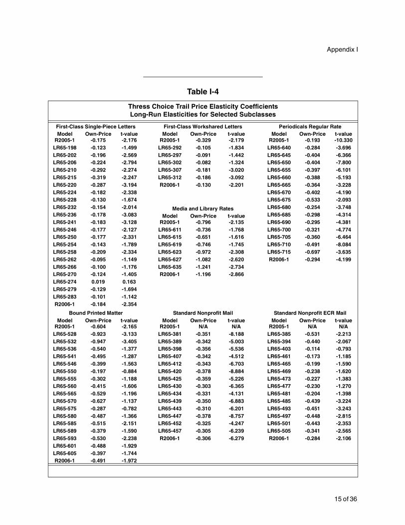
Appendix I
Table I-4
Thress Choice Trail Price Elasticity CoefficientsLong-Run Elasticities for Selected Subclasses
First-Class Single-Piece Letters First-Class Workshared Letters Periodicals Regular RateModel Own-Price t-value Model Own-Price t-value Model Own-Price t-value
R2005-1 -0.175 -2.176 R2005-1 -0.329 -2.179 R2005-1 -0.193 -10.330LR65-198 -0.123 -1.499 LR65-292 -0.105 -1.834 LR65-640 -0.284 -3.696LR65-202 -0.196 -2.569 LR65-297 -0.091 -1.442 LR65-645 -0.404 -6.366LR65-206 -0.224 -2.794 LR65-302 -0.082 -1.324 LR65-650 -0.404 -7.800LR65-210 -0.292 -2.274 LR65-307 -0.181 -3.020 LR65-655 -0.397 -6.101LR65-215 -0.319 -2.247 LR65-312 -0.186 -3.092 LR65-660 -0.388 -5.193LR65-220 -0.287 -3.194 R2006-1 -0.130 -2.201 LR65-665 -0.364 -3.228LR65-224 -0.182 -2.338 LR65-670 -0.402 -4.190LR65-228 -0.130 -1.674 LR65-675 -0.533 -2.093LR65-232 -0.154 -2.014 Media and Library Rates LR65-680 -0.254 -3.748LR65-236 -0.178 -3.083 Model Own-Price t-value LR65-685 -0.298 -4.314LR65-241 -0.183 -3.128 R2005-1 -0.796 -2.135 LR65-690 -0.295 -4.381LR65-246 -0.177 -2.127 LR65-611 -0.736 -1.768 LR65-700 -0.321 -4.774LR65-250 -0.177 -2.331 LR65-615 -0.651 -1.616 LR65-705 -0.360 -6.464LR65-254 -0.143 -1.789 LR65-619 -0.746 -1.745 LR65-710 -0.491 -8.084LR65-258 -0.209 -2.334 LR65-623 -0.972 -2.308 LR65-715 -0.697 -3.635LR65-262 -0.095 -1.149 LR65-627 -1.082 -2.620 R2006-1 -0.294 -4.199LR65-266 -0.100 -1.176 LR65-635 -1.241 -2.734LR65-270 -0.124 -1.405 R2006-1 -1.196 -2.866LR65-274 0.019 0.163LR65-279 -0.129 -1.694LR65-283 -0.101 -1.142R2006-1 -0.184 -2.354
Bound Printed Matter Standard Nonprofit Mail Standard Nonprofit ECR MailModel Own-Price t-value Model Own-Price t-value Model Own-Price t-value
R2005-1 -0.604 -2.165 R2005-1 N/A N/A R2005-1 N/A N/ALR65-528 -0.923 -3.133 LR65-381 -0.351 -8.188 LR65-385 -0.531 -2.213LR65-532 -0.947 -3.405 LR65-389 -0.342 -5.003 LR65-394 -0.440 -2.067LR65-536 -0.540 -1.377 LR65-398 -0.356 -5.536 LR65-403 -0.114 -0.793LR65-541 -0.495 -1.287 LR65-407 -0.342 -4.512 LR65-461 -0.173 -1.185LR65-546 -0.399 -1.563 LR65-412 -0.343 -6.703 LR65-465 -0.199 -1.590LR65-550 -0.197 -0.884 LR65-420 -0.378 -8.884 LR65-469 -0.238 -1.620LR65-555 -0.302 -1.188 LR65-425 -0.359 -5.226 LR65-473 -0.227 -1.383LR65-560 -0.415 -1.606 LR65-430 -0.303 -6.365 LR65-477 -0.230 -1.270LR65-565 -0.529 -1.196 LR65-434 -0.331 -4.131 LR65-481 -0.204 -1.398LR65-570 -0.627 -1.137 LR65-439 -0.350 -6.883 LR65-485 -0.439 -3.224LR65-575 -0.287 -0.782 LR65-443 -0.310 -6.201 LR65-493 -0.451 -3.243LR65-580 -0.487 -1.366 LR65-447 -0.378 -8.757 LR65-497 -0.448 -2.815LR65-585 -0.515 -2.151 LR65-452 -0.325 -4.247 LR65-501 -0.443 -2.353LR65-589 -0.379 -1.590 LR65-457 -0.305 -6.239 LR65-505 -0.341 -2.565LR65-593 -0.530 -2.238 R2006-1 -0.306 -6.279 R2006-1 -0.284 -2.106LR65-601 -0.488 -1.929LR65-605 -0.397 -1.744R2006-1 -0.491 -1.972
15 of 36
Docket No. R2006-1
warning that should have alerted readers to the difference in definitions. See USPS-T-7
at 38.
[29] Calculations of price elasticities for three alternative definitions are shown in
Table 3. The alternative definitions are:
• Thress’ “Long-Run Own-Price” Elasticity (“Own-Price” in Table I-3) – The ratio of the percentage change in volume to the percentage change in price with all other rates and discounts in the demand equation held fixed. This definition implicitly assumes that the two rates that are used to calculate a worksharing discount always change by the same amount leaving the discount unchanged. Thress’ own-price elasticities are best-suited for judging the impact of rate changes under the efficient component pricing (ECP) rule. Under this rule, the discount is set equal to the per-piece cost saving of worksharing to the Postal Service.
• Combined Price Elasticity (“Combined Price/Discount Elasticity” in Table I-3) – The ratio of the percentage change in volume to an equal percentage change in all of the postal rates and discounts in the demand equation. This elasticity can be calculated by simply summing the coefficient estimates for all of the postal rates and discounts appearing in Thress’ log-log demand equations. The definition implicitly assumes that the two rates that are used to calculate a worksharing discount always change by the same percentage amount. Therefore, the discount will also change by the same percentage. The combined price elasticity is best-suited for estimating the impact of inflation while nominal postal rates remain fixed. Then, all real postal rates and discounts change inversely in proportion to the general level of prices. The combined price elasticity is also useful for judging the effects of across-the-board changes in rates, e.g., a proportionate change in all First-Class rates.
• Standard Economic Definition of Elasticity (“Price Elasticity @2005 Rates” in Table I-3) – The ratio of the percentage change in volume to the percentage change in price with all other rates (but not discounts) in the demand equation held fixed. This definition implicitly assumes that a worksharing discount will increase or decrease by an amount equal to the change in price. The formula
for a discount, , used by witness Thress is the arithmetic difference
between the rates for the discounted, , and undiscounted, , categories
of service, . If the demand equation is for the discounted
category then the discount decreases as the rate increases. If the demand equation is for the undiscounted category then the discount and the rate increase together. The standard economic elasticity is a function of the ratio of the price to the discount and can be calculated for an assumed
price and discount using the formula: .
DP1 P2
D P2 P1–=
P D E E0 ED P D⁄( )+=
16 of 36

Appendix I
and are the own-price and discount elasticities from Thress’ fitted
equations.
[30] Table 3 shows that there can be a considerable difference in the price
elasticities depending upon how they are defined. For example, for Docket No. R2006-1,
the various price elasticities for First-Class single-piece letters are -0.184 (Thress’
Long-Run Own-Price), -0.280 (Combined) and -0.730 (Standard Economic Definition).
Elasticities calculated using the standard economic definition in Table 3 use the
before-rates postal rates and discounts in the formula .
4. Did witness Thress commit any fatal technical mistakes?
[31] The application of appropriate econometric methods to fit equations that
correctly represents the demand behavior of postal customers ensures that the fitted
models will have properties that are known and desirable. For the estimates of the price
elasticities, the most important of these properties are that the estimates are consistent
(unbiased in the limit) and that the estimates have sampling distributions that are known
at least approximately. Standard econometric methods are also usually efficient in their
use of data whereas improvised methods often waste information leaving estimates that
are statistically less accurate. The Commission depends upon these properties to
evaluate the reliability of the forecasts and the accuracy of the price elasticities it uses.
Incorrect models and methods make it difficult for the Commission to employ any of the
standard statistics that should describe a fitted model’s reliability and accuracy such as
witness Thress’ MSEs and t-values.
[32] The use of novel and/or improvised estimation methods are discouraged by
the Commission’s rules of practice and procedure. Under these rules, such methods
must be accompanied by “a description and analysis of the technique that is sufficient for
a technical evaluation.” Standard methods need only be accompanied by “a reference to
a detailed description in a text, manual, or technical journal” and a justification for using
the technique. See 39 § 3001.31.k(2)(iv)(e)
E0 ED
E E0 ED P D⁄( )+=
17 of 36

Docket No. R2006-1
[33] The testimony of GCA witness Kelejian identifies several aspects of witness
Thress’ econometric practice that may constitute technical errors. Witness Kelejian’s
comments and criticisms apply to the methods used by witness Thress to fit many of the
demand equations of the Postal Service models.
• Witness Thress applies a Box-Cox transform to several variables used in the models to capture the effects of electronic diversion of mail via the Internet. The Internet variables used by witness Thress all have recorded values beginning after the start of his time series samples. The Box-Cox transform is a frequently-used method for avoiding a singularity when using such variables in a log-log equation. Unfortunately, witness Thress has oversimplified the transform in several of the demand equations. This causes an omission of explanatory terms from the fitted equation. GCA-T-5 at 3-7.
• Witness Thress uses an improvised preliminary statistical procedure to find a value for a nonlinear parameter required for each of his Box-Cox transforms. The effect of this preliminary procedure on the properties of his final estimates is unknown.
• Witness Thress imposes two kinds of symmetry conditions on his parameter estimates. First, he assumes that volume flows in response to discount changes between worksharing and non-worksharing subclasses are symmetric. And, second, he imposes the Slutsky-Schultz symmetry condition on the cross-elasticities of postal services that are regarded as close substitutes. Witness Kelejian points out that Thress’ method for imposing these symmetry conditions creates explanatory variables in his equations that are observed with an error. This will result in inconsistent estimates of the equation’s coefficients. Id. at 6-12.
• Witness Thress’ method for imposing symmetry conditions has the effect of adding stochastic restrictions to his samples. However, the stochastic restrictions do not have autocorrelated errors as do the equations. This creates a conflict between his method for imposing the symmetry conditions and his method for treating autocorrelated disturbances. Id. at 12-14.
• Witness Thress’ treatment of autocorrelated equation errors always omits the 3-quarter lagged error and frequently omits one or more of the other lagged errors for an autoregressive process over four quarters (AR-4). Id.
• Witness Thress selects his preferred models from among the set of candidate models on the basis of the MSE of the fits. The preferred model is the one with the minimum MSE. Witness Kelejian points out that model selection on the basis of the minimum MSE can lead to the selection of an incorrect model even if the correct model is among those in the set of candidates. Id. at 14-15.
[34] In addition, GCA asserts on Brief that the use of MSE as the criterion for
model selection violates the Commission’s rules of practice and procedure because it is
18 of 36

Appendix I
neither referenced nor described in reviewable detail by witness Thress. GCA Brief at
43-47.
[35] In his defense, witness Thress performed a limited number of additional
equation fits and conducted various statistical tests reported in his rebuttal testimony.
USPS-RT-2 at 50-60. The intent of this additional work was to demonstrate that the
impact on the coefficient estimates of the technical issues raised by witness Kelegian is
small. Minor mistakes in the specification of an equation or the application of
econometric methods can be expected to have a correspondingly minor impact on
estimates. The impact will also tend to be small if the estimates are robust. Witness
Thress is able to show, with respect to First-Class single-piece letters, that correcting
most of the practices criticized by witness Kelejian would have very little impact on the
estimates of own-price and discount elasticities.
[36] His models are the only comprehensive set available for the Commission’s
use in this proceeding. Witness Clifton has fit equations that might be used to replace
the models for First-Class single-piece letters and Standard Regular mail. Otherwise,
the Commission has no alternative except to use one or another of the models fit by
witness Thress. No party has offered testimony that any of the other models fit by
witness Thress and catalogued in library reference USPS-LR-L-65 are superior to those
he has selected to make the volume forecasts.
[37] The Commission’s findings with respect to witness Thress’ econometric
practice are:
• Witness Thress’ econometric practice is conventional except with regard to several devices that have been adopted to deal with the special problems he confronts: 1) finding suitable variables to describe the role of the Internet in the electronic diversion of mail; 2) imposing symmetry conditions on his estimates of discount elasticities and cross-price elasticities; and 3) using the Shiller lag method to fit lag structures for the price elasticities. Without these complications his estimates would be the result of conventional applications of the method of generalized least squares.
• Witness Kelejian has correctly pointed out several ways that witness Thress’ econometric practice is problematic. However, it has not been demonstrated that the mistakes will have more than a very minor impact on the volume forecasts made with the models. It appears likely to the Commission that the
19 of 36
Docket No. R2006-1
principal effect of most of the mistakes will be to cause inconsistencies in the estimates of the less stable price elasticities. Most of the technical mistakes noted by witness Kelejian are minor and should have correspondingly minor consequences.
• The dangers of using MSE as a model selection criterion are well-known from the literature on stepwise regression where minimizing MSE along the steps is the most commonly used rule for selecting variables to enter or leave the regression. Choosing a model with the lowest MSE from among a set of non-nested models, as witness Thress has done, is defensible as a means of selecting a model that will make forecasts with a small error variance. However, the chosen model is likely to be somewhat mis-specified. For example, variables with t-value that are less than 1.0 in absolute value are usually omitted from the equation.
5. Does the Postal Service model underestimate the price sensitivity of First-Class single-piece letters?
[38] GCA witness Clifton asserts that the own-price elasticity of First-Class
single-piece letters has been underestimated while that of Standard Regular mail has
been overestimated. GCA-T-1 at 2-3. In an efficient rate design, subclasses with lower
(absolutely) price elasticities would tend to be assigned higher markups over marginal
costs than those subclasses with higher price elasticities. For example, in the simplest
application of Ramsey pricing the markups are inversely proportional to the own-price
elasticities. Therefore, witness Clifton’s claim supports GCA’s recommendation that the
Commission raise the First-Class single-piece letter rate by one cent less than the Postal
Service has proposed and make up the lost revenue by further raising the rates for
commercial bulk mailers.
[39] The GCA argues that First Class single-piece mail is declining due to
electronic diversion, and that mail volumes lost to diversion will not subsequently return
to the system. GCA Brief at 5. As a result, GCA argues that demand for single-piece
First-Class Mail is much more price sensitive than reflected in the own-price elasticity
estimated by witness Thress. USPS Brief at 37-38; see also, generally, USPS-T-7.
asserts that high institutional cost burdens on First-Class should be moderated in an
20 of 36

Appendix I
environment where the preponderance of mail is shifting to Standard Mail GCA. Brief at
2, 4.
[40] The arguments that apply to GCA’s claim are found in the testimony of GCA
witnesses Clifton (GCA-T-1) and Martin (GCA-T-2). The testimony of Postal Service
witnesses Thress (USPS-T-7 and USPS-RT-2) and Bernstein (USPS-T-6) and GCA
witness Kelejian (GCA-T-5) are also relevant. The following points summarize the
argument and evidence.
• The price elasticity of demand for a single producer’s product is generally higher (absolutely) if the producer has competitors offering products that are close substitutes than if he does not. The Postal Service now has a newly emerged competitor in what witness Clifton describes as the “payments” market. Clifton’s Federal Reserve data, Bernstein’s diary studies and Martin’s surveys all show that bill payments are increasingly being made electronically, often over the Internet, while bill payments by check remitted in First-Class single-piece letters are declining.
• Witness Clifton makes non-econometric estimates of price elasticities for bill payments that are higher than the own-price elasticity estimate from the Postal Service model for First-Class single-piece letters. GCA-T-1 at 20.
• Witness Martin’s surveys suggest a weak connection between the use of the mail for bill payments and postal rates. His hypothesis is that rate increases act as a trigger encouraging consumers to reconsider their customary use of the mail to pay bills.
• Witness Clifton notes that witness Thress’ estimates of own-price elasticities for First-Class single-piece letters have changed considerably from case to case since Docket No. R97-1 as shown in Table I-3. GCA-T-1 at 4-11. This instability in the price coefficients is attributed to changes witness Thress has made in the demand equation to represent electronic diversion and the increasing impact of the Internet on volumes.
• Witness Clifton claims that witness Thress’ incorrect application of the Box-Cox transform to the Internet variable in his equation for First-Class single-piece letters causes a downward bias in the own-price elasticity. GCA-T-1 at 33. In fact, all of the mistakes cited by witness Kelejian are likely to produce more-or-less biased estimates of the coefficients in the Postal Service models. However, it is not usually possible to determine the direction of these biases. Witness Thress’ technical problems are not serious if the biases they leave can be expected to be small.
• Volume forecasts made for First-Class single-piece letters using the Postal Service models for recent rate proceedings have all proven too high. The percentage errors for Docket Nos. R2000-1, R2001-1 and R2005-1 are all negative. Witness Clifton demonstrates that the discrepancy can be
21 of 36

Docket No. R2006-1
corrected for the Docket No. R2000-1 forecasts by assuming a higher (absolutely) own-price elasticity for First-Class single-piece letters. Id. at 41-43.
• Witness Thress’ demand equations are log-log equations with constant own-price elasticities. Witness Clifton points out that if the equations are actually linear the own-price elasticity will increase as volume decreases. First-Class single-piece letters per person have been declining since 1996 and are forecast to continue declining. With a linear demand equation this would raise the own-price elasticity of First-Class single-piece letters. Id. at 45-49.
• Witness Clifton fits linear analogues of witness Thress’ demand equations for First-Class single-piece letters from Docket Nos. R2005-1 and R2006-1 and finds that the estimated own-price elasticities increase substantially. A similar experiment with Standard Regular mail results in a decrease in the estimated own-price elasticities. Id. at 49-56.
[41] In his defense of the price elasticity estimates, witness Thress points out that
there are no certain grounds in economic theory for presuming a priori that the
opportunity for electronic diversion afforded by the Internet will increase the own-price
elasticity of First-Class single-piece letters. Market bifurcation can produce the opposite
result. USPS-RT-2 at 12-15. If the postal customers who are diverted have high price
elasticities while the ones that continue to use the mail have low elasticities, then the
aggregate own-price elasticity will decrease rather than increase. Therefore, it is
impossible to determine on purely conceptual grounds if the own-price elasticity of
First-Class single-piece letters has increased.
[42] The question is an empirical issue that can only be resolved by gathering the
quantitative evidence, doing the required econometrics and employing the appropriate
statistical tests. The testimony proffered by GCA witnesses Clifton and Martin simply
does not do this job. Witness Clifton’s statistics drawn from Federal Reserve data and
other sources is suggestive, but is hardly conclusive with respect to the own-price
elasticities. Price elasticities can not be derived non-econometrically, as he has
attempted, from this data. Nor can a change in own-price elasticities be inferred from
witness Martin’s survey responses, even if we are willing to accept completely his trigger
theory and other explanations for the responses.
22 of 36

Appendix I
[43] The questionnaire, data capture and sample designs for the consumer and
small business surveys referenced by witness Martin precluded an objective examination
of “emerging competitive substitutes to first class letter mail.” GCA-T2-1. The
qualifications associated with the results of these studies should be noted carefully.
While the data presented by witness Martin confirmed increased acceptance of
technological advances accessible to the general consumer and a gradual shift toward
more use of electronic alternatives to First-Class Mail, his efforts to provide data
supportive of the hypothesis that knowledge of regularly scheduled increases in postage
rates would “trigger” a switch or serious consideration of a switch to electronic methods
of submitting billing statements and rendering payment were substantially deficient. His
major conclusions were subjective and lacked statistical defensibility.
[44] There is little disagreement between Postal Service and GCA witnesses
regarding the negative impact of electronic diversion on First-Class single-piece volumes
and the facilitating role of the Internet. All of the available information tells roughly the
same story. Since the Internet became widely accessible in the mid-1990s, it has been
used to conduct an increasing volume of transactions that were formerly conducted by
mail. The replacement of check-in-the-mail bill payments by electronic bill payments
over the Internet receives the most attention in testimony. However, it is not possible to
tell if the well-documented loss of volume to the Internet is evidence that the own-price
elasticity of First-Class single-piece letters has increased with the advent of the Internet.
6. Testimony of Witnesses Clifton and Kelejian
[45] Witness Kelejian’s identification of errors in the econometrics and witness
Clifton’s observation that witness Thress’ estimates are unstable fall short of proving that
the own-price elasticity of First-Class single-piece mail has increased. Most of the
mistakes identified by witness Kelejian are likely to cause biases in the estimates of the
own-price elasticities as well as the other coefficients of witness Thress’ First-Class
single-piece equation. However, there is no reason to believe that the biases will
23 of 36

Docket No. R2006-1
necessarily result in an underestimate. The same can be said regarding the instability of
the estimates with respect to witness Thress’ various experiments defining an Internet
variable. Witness Thress’ elasticity estimates for First-Class single-piece letters are not
robust. Altering the Internet variable in the equation can produce a considerable change
in the estimated own-price elasticity. However, we simply cannot tell if the right definition
will leave a higher or lower estimate of the own-price elasticity for First-Class
single-piece letters.
[46] Nor can the Commission determine from the evidence if there has been an
increase in the own-price elasticity over the time period spanned by witness Thress’
sample (1983 Quarter 1-2005 Quarter 4). None of the econometric research presented
in testimony proceeds towards a formal statistical test of this hypothesis. Witness
Thress’ log-log equations do not include any mechanism that would permit the own-price
elasticities to change over the time span of his samples. If the First-Class single-piece
letters own-price elasticity has risen recently, witness Thress’ estimates will average
them with the lower elasticities of earlier years. Witness Clifton’s linear equations do the
same with the slope coefficients for rates. Both Thress’ and Clifton’s models could be
modified in several ways and refit to test the hypothesis that the own-price elasticity of
First-Class single-piece letters has increased as the Internet has diverted larger volumes
of mail. But neither witness has done this work.
[47] Witness Clifton’s linear equations for First-Class single-piece letters and
Standard Regular mail are simpler and somewhat easier to fit than witness Thress’
log-log (Constant Elasticity of Substitution (CES)) equations because there is no need to
perform a Box-Cox transformation on the Internet variables. Since witness Thress’
own-price estimates are not robust for either of his equations, it is not surprising that the
change in the equation form produces very different own-price elasticities. Again, this is
not proof that the own-price elasticity of First-Class single-piece letters is higher
(absolutely) than witness Thress’ estimate or that the own-price elasticity of Standard
Regular mail is lower. It is just further evidence of instability.
24 of 36

Appendix I
[48] Witness Clifton’s estimates are also somewhat suspect on technical
grounds. He has chosen a very defective method for dealing with autocorrelated errors
and his estimate of the coefficient for the worksharing discount from his equation for
First-Class single-piece letters has a sign that can not be correct. (USPS-RT-2 at 37-45)
The latter flaw indicates that the equation is mis-specified.
7. Testimony of Witness Martin
[49] GCA witness Martin’s market research study attempts to show that
electronic substitution for delivery of material ordinarily carried as First-Class Mail has
made mail more price-sensitive. USPS Brief at 38.
[50] Witness Martin said “postal rates seem to be a future trigger for diverting
from mailed bill payments.” GCA-T-2 at 23. Martin implies that more widespread
broadband access provides an increasing number of bill-payers an option to switch
irreversibly to electronic bill payment/presentment, and that the existence of this
switchover phenomenon exacerbates the effective elasticity of First-Class Mail. Martin
also implies that it is the disruptive effect of a price change itself irrespective of the
amount that can “trigger” single-piece mailers to adopt electronic alternatives. He
suggests that both price itself as well as the “trigger” event of price changes can speed
the transition to electronic bill payment. GCA argues that “the frequency and magnitude
of [First-Class letter mail] rate increases are likely to be important behavioral triggers as
regards consumer decisions to shift First-Class letter mail volumes to electronic
substitutes” and that “price matters.” GCA Brief at 5. Martin also says “[t]hat data
suggest that once motivated to switch from the mailed payments by the price (or
changes in the price) of postage, major mailers then use other competitive attributes for
the switching or diversion decision.” GCA-T-2 at 27.
[51] GCA acknowledges the “general consensus that the First-Class [mail]
volumes that have left the Postal System due to electronic diversion will not return.”
GCA Brief at 63. GCA also asserts that its proposal is likely to stem further migration by
25 of 36

Docket No. R2006-1
mailers who still use single piece First-Class mail. GCA Brief at 34-37. GCA uses
Martin’s testimony to highlight the significance of price in the decision to switch.
However, the Postal Service points out that Martin’s survey results show that for every
category of respondents, postal rate changes were rated the least important factor (of ten
factors) in selecting payment method.
[52] In opposition, the Postal Service argues that Martin failed to consider the
extent and magnitude of electronic diversion without any postal rate increases. The
Service also says Martin acknowledged that previous researchers have not addressed
postal rates as a factor in assessing transition to electronic alternatives to mail. GCA-T-2
at 1, cited in USPS Brief at 38-40. The Service says that Martin omits any study of the
case in which postage rates remain the same. The Postal Service points to witness
Bernstein, who said that he believes factors other than postal rates are dominant in
terms of explaining the growth in electronic alternatives, because he has seen numerous
studies on the subject that do not mention postal rates. USPS Brief at 40, citing Tr.
6/1443-44.
[53] The Postal Service says that witness Spulber in Docket No. R94-1 and
witness Sidak in Docket No. R2006-1 both testified that electronic alternatives are
encouraged by the increasing benefits and declining cost of electronic transmission,
rather than rising postal rates. USPS Brief at 40-41, citing AMMA, et al.-RT-2 at 12,
Docket No. R94-1, Tr. 19/9195 and Docket No. R2006-1, Tr. 32/10873-77 passim.
Witness Sidak says that the increasing benefits and declining costs of electronic
transmission which are responsible for its rapid expansion are “pretty uncontroversial”
(Tr. 32/10876) and that he has no basis to disagree with Spulber’s contention that these
developments are independent of postal rates. Id. While Martin’s failure to explain the
omission in other studies of postal rates as a significant factor in diversion to electronic
alternatives is not by itself fatal to his argument, it certainly suggests a substantial gap in
his analysis and research that would require a higher standard of evidentiary support.
[54] Witness Martin utilized certain survey questions to assess the importance of
postal rates in diversion to electronic alternatives to mail. GCA-T-2 passim. The Postal
26 of 36

Appendix I
Service argues that the questions are impossibly flawed and inartfully drafted so as to
preclude any meaningful interpretation of the results. USPS Brief at 50. One of the
survey questions does not specify the magnitude of postal increases upon which the
respondent is assessing the likelihood of switching. Another survey question specifies a
series of potential postal increases, but does not specify the time frame involved. Id. at
50-51.
[55] The Service also expresses concern about the order in which the survey
questions were posed. It says that the trigger questions were asked after, not before, the
competitive factors questions, preventing the proper analysis of possible connections
between the decision to switch and postal rates. The Service argues that Martin’s
decision to limit his inquiry to changes in postal rates and avoid other potential switching
factors destroyed his ability to draw meaningful conclusions from his survey. Id. at
47-49. The questions also sought from the respondents whether they would “seriously
consider switching” to some form of electronic payment instead of the mail. The Postal
Service questions whether “seriously consider switching” can be equated with “will
switch,” and concludes that it can not. Id. at 53.
[56] The questionnaires for the consumer and small business surveys, on which
Martin placed considerable emphasis, were clearly biased toward responses suggesting
that an increase in the postage rate for First-Class Mail would engender a change in the
mode of billing for businesses and bill payment for consumers. This was the result of
emphasizing perceived knowledge of future postal rate increases, as a potential
significant factor affecting the diversion of bill payment and billing from mail, in the
phrasing of selected questions. The questionnaire designs employed by witness Martin
did not permit the collection of data that would examine the tendency toward greater use
of electronic options as a preference to mail in the absence of increases in postal rates.
[57] The Service questions Martin’s selection of defined price points. Id. at 54.
Martin’s selection of defined price points used for the survey made the study vulnerable
to central tendency bias, in which respondents are reluctant to choose the extreme
values offered in such a survey and tend to select more moderate values.
27 of 36

Docket No. R2006-1
[58] Apart from being suggestive, the questions that Martin posed to derived data
on the threshold postal rate increase that would lead to serious consideration of a
diversion from the use of mail were ambiguous and possibly misleading. See, e.g.,
GCA-T-2 at 25. There was no time frame associated with the increases and there is no
definitive method of identifying the likelihood that giving serious consideration would
actually result in switching to an alternative to First-Class Mail.
[59] The Commission believes that the questions regarding “seriously consider
switching” are biased since they allude to whether the respondent expresses an actual
intent to switch, or instead simply acknowledges a measure of willingness to consider a
new idea.
[60] Martin suggests that the mere occurrence of a change in the First-Class
postage rate, independent of its magnitude, acts as an incentive to switching to
electronic bill payment. There is no basis for discounting entirely the possibility that
Martin’s hypothesis has some intrinsic merit. Nevertheless, his research approach
appears sufficiently flawed and his stated conclusions are unsupported by his factual
data.
[61] Martin characterized his telephone survey of consumers as a national
random sample of 1,000 household bill payers. Id. at 15. To the extent that the targeted
household did not have telephone numbers in the sampling frame for the survey, there is
selection bias associated with the subsequent estimates. In addition, a table entry
indicating that only 6.4 percent of the bill payers in the survey were college graduates ,
suggests a large sampling error, serious frame bias and/or non-response bias, or both.
See GCA-T-2 at 18, Table 2. Moreover, while the sample size for the survey is given as
1,000, the actual response rates were not provided for most of the tables and questions
presented in the testimony. The Commission finds that the sample design was
insufficiently rigorous for the conclusions drawn.
[62] In market research and the general conduct of a survey, probability sampling
and probability sampling designs can be used to make valid inferences about a
population. Most of the primary conclusions drawn by witness Martin are based on the
28 of 36

Appendix I
results of Likert2 scale ratings for selected questions. Interpreting Likert scale ratings
without sufficient care can introduce sources of error. One source of interpretive error is
arbitrarily assigning a specific Likert response to a particular conclusion. Martin
arbitrarily assumed that a rating in a specific range should be interpreted as the certainty
of the occurrence of a given event. For example, for the question relating to the
likelihood of switching to electronic bill payments in light of pending regularly scheduled
postal rate increases, a rating of 5 or more was treated as a definite decision to switch for
estimation purposes. Consequently, Martin concludes that 25 percent of “the critical
market segment” of major mailers would probably switch to electronic payment. The
Commission has no objective and valid method of assigning the probability or likelihood
of a switch given a specific Likert rating, nor can we objectively assess the reliability of
the “principal estimates” provided by Martin.
[63] Martin contends that for the three mailing segments he characterized as
“major,” “minor,” and “hardcore” mailers, the perception of planned regular increases in
the First-Class postage rate for bill paying would trigger a switch to electronic payments
and billing. He makes this contention despite the fact that each of these groups
considered future postal rate increases to be the least important among factors that
could potentially affect their decision regarding the method of bill payment. Moreover,
historical data suggest the absence of significant correlation between the decline of
traditional mail payment and the rate of increase in First-Class postage.
8. Can the Postal Service demand models be improved?
[64] Fitting an aggregate demand function to a time series sample for a single
supplier and a single product with predetermined prices is one of the most common
2 A Likert Scale is a type of psychometric response scale often used in questionnaires, and is the most widely used scale used in survey research. Martin reports using a 7 point Likert scale to measure switching receptivity in order to assess the vulnerability of types of First-Class Mail to electronic diversion. GCA-T-2 at 49.
29 of 36

Docket No. R2006-1
applications in econometrics. The most useful equation forms, variable definitions, and
estimation methods are the grist for every standard textbook and econometrics manual.
The markets for postal services have generally enjoyed a stable existence for many
years and fairly accurate statistics for U.S. postal volumes and prices have been
collected on a quarterly basis since 1972. Fitting postal demand models should be
straightforward. Yet almost all of the equations of the Postal Service demand models
have unusual structural features that require highly specialized methods. These
structural features are:
• Lagged price coefficients requiring the Schiller lag estimator;
• Box-Cox transforms of Internet variables requiring a nonlinear estimator;
• Symmetry conditions requiring estimation with stochastic restrictions; and
• Autocorrelated disturbances requiring the Cochrane-Orcutt procedure.
[65] There are many studies of the demand for postal services. Hausman
(1987), Taylor (1989), and Pearsall (1997, 2002 and 2005) have all fit demand models
using U.S. Postal Service quarterly time series data. Wolak (1997 and 1998) has fit
models to cross-sections drawn from the U.S. Census. Robinson (2006) cites 20
European demand studies that have appeared in open literature. Many of these studies
are reported in chapters of Crew and Kleindorfer’s annual Postal and Delivery
Economics Conference volumes. A list of relevant references is provided at the
conclusion of this Appendix.
[66] No references or apparent uses of any postal demand research other than
the models fit by himself and his colleagues for previous rate proceedings or the
competing models of witness Clifton are made by witness Thress in his testimony. Other
researchers have successfully modeled the demand behavior of postal customers with
far simpler models than those fit by witness Thress. Other researchers also tend to fit
models that are less specialized with respect to different classes and categories of mail.
The structural features that complicate the estimation of witness Thress’ equations, with
the exception of autocorrolated disturbances, are absent from the models fit by other
30 of 36

Appendix I
researchers. And, other researchers have identified significant causes of variation in
postal volumes that have been entirely overlooked by witness Thress. For example, the
Postal Service models all incorporate fixed seasonals, but Pearsall (2005) found that the
seasonals for most subclasses are changing over time. Some of the findings of other
researchers ought to be useful in simplifying and improving the models fit for rate
proceedings by Postal Service econometricians.
[67] In general, witness Thress attempts to fit large models with his samples.
Often this leaves few degrees of freedom for the estimate of the MSE. For example, his
model for Periodicals Outside County rates has 23 parameters and is fit to a sample of
52 quarterly observations leaving only 29 degrees of freedom. Fitting large models to
small samples is also difficult because of the likelihood that the explanatory variables will
be correlated in the sample. Near multi-colinearity will often cause the coefficient
estimates of the correlated variables to be inaccurate and non-robust.
[68] The majority of the parameters found in the Postal Service models are fixed
seasonals. Up to 22 variables are included in the demand equations to model seasonal
effects down to the level of the five days before Christmas. For example, 12 of the
parameters in the model for Periodicals Outside County rate are seasonal coefficients.
The volume forecasts for a rate proceeding are made by government quarters and make
no use of this detail in the estimation of seasonal variations in volume. A set of three
dummy variables are all that are needed to represent fixed seasonal effects for a model
that is used to make quarterly forecasts. Little precision is likely to be gained for the
forecasts by adding dummy variables to more finely divide the year.
[69] Own-prices appear in the Postal Service models lagged up to four quarters.
The explanation that has been provided for this mechanism is that postal customers
require time, up to five quarters, to respond to changes in postal prices. The assumption
that underlies this explanation is that postal customers are surprised by rate changes.
However, when rate changes are fully expected, postal customers should respond
without appreciable delay. Most changes in relative postal rates are widely reported and
easily anticipated. They are the result of generalized price inflation and changes to
31 of 36

Docket No. R2006-1
nominal rates made after more than 12 months of public consideration by the Postal
Service and the Commission. Business mailers are aware of future rate changes and
even retail postal customers are provided some advance notice.
[70] The lag structure assumed for most postal price effects is rarely justified by
the fits of the Postal Service models. Most often the lag structure is the result of using
the Shiller lag method to force the coefficients to lie along a polynomial and to all have
non-positive values. Frequently, the lag structure is simply imposed by assumption.
Getting the lag structure right (if there are lagged responses to rate changes) is important
for forecasting volumes accurately in the test year because the time span between the
date the rates are assumed to take effect and the beginning of the test year is less than
five quarters. For this case, the rates are expected to take effect on May 6, 2007, and
the test year begins on October 1, 2007. Under the lag structure estimated by witness
Thress, postal customers will not fully respond to the Commission’s recommended rates
until the test year is almost over.
[71] Witness Thress’ symmetry assumptions not only cause estimation issues,
they may be incorrect on economic grounds as well. Witness Kelejian notes that the
assumed symmetry of the volume effects of worksharing discounts between worksharing
and non-worksharing categories is not necessarily correct. The same can be said of the
Slutsky-Schultz symmetry condition. This condition arises from the mathematics of
utility-maximizing behavior by individual consumers. However, it is far from clear that the
same symmetry applies to the aggregate behavior of all consumers of postal services.
[72] There are no economic causes identified for some of the dummy variables
and trends that witness Thress inserts in several of the subclass demand equations.
Several examples of this practice are: (1) a dummy variable equal to one beginning in
2001 Q3 inserted in the equations for Standard ECR mail and Express Mail; (2) a linear
trend beginning in 2001 Q3 inserted in the equations for Express Mail and Priority Mail;
(3) a linear trend for the period 1990 Q1 through 2001 Q2 in the Priority Mail equation;
(4) a dummy variable equal to one beginning in 2004 Q1 in the Destination Entry Parcel
32 of 36

Appendix I
Post equation; and (5) a dummy variable equal to one beginning in 1998 Q1 in the
equation for Bound Printed Matter.
[73] Witness Kelejian has noticed that the autoregressive processes that witness
Thress assumes for many of the equation disturbances always omit the third quarter lag
and sometimes omit other lags as well. GCA-T-5 at 12-14. These are odd processes to
find in an economic model. Autoregressive error processes are often present in models
fit to time series data because the causes of disturbances can persist over time or recur
periodically. The autoregressive process that this suggests for postal demand equations
is a process with all four lags included.
[74] Although they are mathematically elegant, the Postal Service worksharing
share models are not a statistical success. Econometrically fit share models are
currently used only to divide the volumes of worksharing categories into their automated
and non-automated components. Other divisions of worksharing categories are made
simply by assuming that the shares observed in the base year will remain fixed. It may
be possible to fit share equations based on logit or probit models that will do better than
this.
9. Can the forecasts be improved?
[75] The Postal Service forecasting method is described in detail by witness
Thress in his direct testimony. USPS-T-7 at 331-65. In brief, the method proceeds
through the following steps:
33 of 36

Docket No. R2006-1
(1) Average quarterly volumes by subclass are determined for a base year. Average quarterly values of the explanatory variables in the model are also computed for the base year.
(2) Forecasts are made or obtained for each explanatory variable of the demand model for each quarter out to one year past the end of the test year.
(3) Multipliers are constructed for each related set of variables using the estimated coefficients and the quarter/average base year ratios of the values of the variables.
(4) The multipliers are applied to the average base year volumes to forecast the volumes for every quarter out to one year past the end of the test year.
(5) Subclass volumes are further split into worksharing rate categories using shares projected with the equations of the shares models.
[76] The forecasting process is called “forecasting off a base year” and is one of
several methods that are commonly used in conjunction with an econometric model
consisting of log-log (CES) equations. The process is an appropriate choice if the errors
in the base year are expected to persist or recur in future quarters because the average
error in the base year is included in the forecasts.
[77] Given the estimated equations of the Postal Service model, the opportunities
available to the Commission to improve the reliability of the test year forecasts are limited
to updating the information used to make them. The Commission might have updated
the information used to make the forecasts in any of the following ways:
• Advance the base year using the additional 3-4 quarters of volumes that are reported in RPWs while a rate proceeding is in progress. The averages for the explanatory variables would also have to be advanced. The base year used by the Postal Service in the current proceeding is GFY 2005. The RPW report for GFY 2006 was released by the Postal Service in December 2006.
• Use more current forecasts of population, economic activity and non-postal prices. The forecasts of these variables used by the Postal Service for this case were made by Global Insight in December 2005. Global Insight updates
34 of 36
Appendix I
these forecasts on a monthly basis and makes major revisions in December of each year.
• Update the projections of explanatory variables, such as the number of broadband subscribers, made by witness Thress. This would have to be done by advancing the forecasts generated by the various models witness Thress uses to make the projections.
[78] In this, as in past proceedings, with the notable exception of Docket No.
R90-1, the Commission has avoided updating the information used to make the volume
forecasts on the grounds that the updating would have little effect. Any improvement in
the accuracy of the volume forecasts would have been outweighed by the inconvenience
to the Postal Service, the parties and the Commission of changing the basis for the
forecasts in mid-proceeding. Updates to projections of economic activity were made in
Docket No. R90-1 to handle the onset of a major recession shortly before the
proceedings ended. The DRI forecasts of economic activity used by the Postal Service
and the Commission at that time showed the recession persisting into the test year. It
was clear that rates based upon the pre-recession DRI forecasts would leave a shortfall
in net revenue during the test year.
[79] We note that the information used by the Postal Service forecast method
was already many months old at the time that the Postal Service submitted its request in
May of 2006. The Postal Service could improve the reliability of the volume forecasts
simply by using the most current available information at the time of filing. It would also
be useful for the Postal Service to revise its forecasts towards the end of a proceeding as
was done in Docket No. R2001-1, or, as an alternative, to make a systematic
presentation all of the information needed to update the forecasts. This would allow the
Commission to more easily determine if an update is necessary.
35 of 36

[80] References
Hausman, J., (1987): Direct Testimony Docket No. R87-1.
Robinson, Alan (2006):”Review Price Elasticity Models for Postal Products,”
Background Paper No. FOM 2006-1, Pitney-Bowes, internal background
papers.
O’Bannon, John H., (1999): “A System of Postal Demands with a Focus on Parcel
Post”, Research Report Presented to U. S. Postal Rate Commission
(manuscript)
Pearsall, Edward S., (2002): Econometric Appendix to Cohen et al “The Impact of
Using Worksharing to Liberalize a Postal Market” in Liberalisation of Postal
Markets, Eds. Gabriele Kulenkampff and Hilke Smit (Rheinbreitbach: Druckerei
Plump KG. Pearsall, Edward S., (2005): The Effects of Worksharing and Other
Product Innovations on U.S. Postal Volumes and Revenues, in Regulatory and
Economic Challenges in the Postal and Delivery Sector, edited by M.A. Crew
and P.R. Kleindorfer, Boston, MA ; Klewer Academic Publishers.
Taylor, Lester D., (1989): Paper prepared for U.S. Postal Rate Commission
Taylor, Lester D., (1993): “The Demand for First-Class Mail: An Econometric
Analysis”, Review of Industrial Organization, Vol. 8., pp. 523-544.
Wolak, F. A., (1997): “Changes in Household-Level Demand for Postal Delivery
Services from 1986 to 1994”, in Managing Change in the Postal and Delivery
Industry edited by M.A. Crew and P.R. Kleindorfer, Boston, MA ; Klewer
Academic Publishers.
Wolak, F. A., (1998): “Electronic Substitution in the Household-Level Demand for
Postal Delivery Services”, in A Communications Cornucopia, ed. Roger G. Nodl
and Monroe E. Price, Washington: Brookings Institution Press.
.

Appendix JMAIL PROCESSING VARIABILITY
1. Summary
[1] For more than two decades, the Postal Service adhered to the view that mail
processing labor costs rise essentially in proportion to the volume of mail that is
processed. This implies that the volume variability of those costs is approximately 100
percent. This view is grounded on the observation by postal experts of the organization
of mailflows and flexibility with which managers typically match labor to those flows. It is
also grounded on the observation that most forms of processing capacity (worker, mail
container, and sorting machine) scale up or down essentially in modular fashion over a
rate cycle. The Commission continues to accept this engineering/operational view of
labor cost variability as realistic and valid.
[2] In Docket No. R97-1, the Postal Service proposed a statistical model for
estimating the variability of mail processing labor costs. The Commission rejected the
proposal. It concluded that the quality of the underlying data were too poor to support a
valid statistical model, that it did not reflect an articulated economic theory, and that the
resulting variabilities (76 percent) were so low as to be implausible. PRC Op. R97-1 at
79-96.
[3] In Docket No. R2000-1, the Postal Service proposed a revised model. While
it reflected a more identifiable economic theory, the theory required a number of
restrictive assumptions that the Commission found to be unrealistic. Prominent among
them was the assumption that each operation within a processing plant functioned as a
stand-alone operation, unaffected by the volume of mail or productivity of any other
operation. Another overly restrictive assumption, in the Commission’s view, was that
piece handlings affect work hours in exactly the same way that volume does. Perhaps
more important, the quality of the underlying data was no better than that upon which the
initial model was based. The resulting variability estimates were even lower (less than 73

Docket No. R2006-1
percent), and as counterintuitive as the initial model results. For these reasons, the
Commission rejected those estimates.
[4] In Docket No. 2005-1, the Postal Service acknowledged for the first time the
possibility that poor data quality was biasing the results of some of its models. In 2002,
Roberts, working on behalf of the OCA, published a paper recommending the use of an
Instrumental Variables estimator to reduce the risk of downward bias that errors in the
measurement of output impart to the class of models that the Postal Service employs. In
that docket, the Postal Service applied the Instrumental Variables technique
recommended by Roberts to its non-automated cost pools. The variabilities estimated for
its manual sorting operations rose dramatically (each by roughly 20 percentage points).
This increased the Postal Service’s estimate of overall mail processing variability to 83
percent. By agreement of the participants to Docket No. R2005-1, the Commission did
not rule on the merits of the cost attribution proposals presented there. Consequently, the
Commission evaluates these revisions to the Postal Service’s proposed models for the
first time in this docket.
[5] Also in this docket, for the first time, the Commission evaluates the approach
to modeling mail processing labor costs recommended by Roberts. He develops a
different theory of production that defines output as the volume of mail processed in the
plant. He believes that approach is needed in order to estimate economically meaningful
marginal costs. He recommends this general approach to the Commission, and
illustrates it with specific variability models for letter sorting and for flat sorting.3 He
concludes that his approach models the variability of letters reasonably well, but not that
of flats. His estimated variabilities for letter sorting operations are well above 100
percent. Also for illustrative purposes, UPS witness Neels presents comprehensive
3 Dr. Roberts’ recommendations are developed in a series of three papers. The first was published in May of 2002 and the second in March of 2006. These papers were made available on the OCA’s portion of the Commission’s website and discussed in public seminars following their publication. Roberts presented testimony in this docket in September 2006 which referenced his findings in the earlier papers and included additional research. These papers have been treated by Roberts and the participants in this docket as an integrated whole in discovery, oral cross-examination, and briefs. The Commission affords them similar treatment in evaluating the evidence in this docket.
2 of 109

Appendix J
models of mail processing that yield variability estimates above 100 percent. A group of
Periodicals mailers “augments” the engineering/operational analysis employed by the
Commission to reflect new data collected by the Postal Service’s In-Office Cost System
(IOCS). The augmented Commission method, the group argues, implies that mail
processing variability ranges from 92 to 94 percent.
[6] As in Docket No. R2000-1, the competing mail processing variability models
in this docket bracket the estimate of approximately 100 percent that the Commission
has traditionally applied to mail processing labor costs. One hundred percent remains
the center of gravity of the array of statistical and the operational estimates of mail
processing variability that have been presented on this and prior records. For this
reason, the Commission adheres to its determination that mail processing labor costs
are almost 100 percent volume variable.
[7] For more than a decade, the Commission has expressed concern that the
quality of the Management Operating Data System (MODS) data upon which mail
processing variability models depend is too poor to support valid statistical models. Over
that time, the quality of that data has not improved in any discernible respect. This
record has clarified the theoretical requirements of valid mail processing models. At the
same time, it illustrates that resourceful data manipulation is not sufficient to overcome
the obstacle to successful modeling that the error-ridden MODS data presents. The
Postal Service should understand that if the quality of the MODS data does not improve,
or alternative data developed, models that rely on such data have little prospect of being
accepted by the Commission.
2. Positions of the Participants
a. The Postal Service’s Revised Mail Processing Model
[8] Since its mail processing labor cost variability model was last litigated in
Docket No. R2000-1, the Postal Service has modified its model in a number of ways.
3 of 109
Docket No. R2006-1
The most significant modification is its use of an Instrumental Variables technique to
estimate the coefficients in these models, following the suggestion contained in the
OCA-sponsored research of Roberts published in May of 2002.4 The Postal Service now
applies this estimating technique to the manual sorting operations, the cancellation
operation, and the Priority Mail operation. To make models of these operations
amenable to the use of the Instrumental Variables, log-linear models have been
substituted for the earlier translog models. The Postal Service continues to use translog
models for the remaining operations.
[9] Witness Bozzo applied the Instrumental Variables approach suggested by
Roberts as a solution to the “potential” inconsistency of variability estimates obtained
from least squares regression techniques “due to measurement error and simultaneity in
MODS output measures.” Docket No. R2005-1, USPS-T-12 at 6. This technique
dramatically altered the variabilities of the manual sorting operations to which they were
applied, as the table below shows.5
[10] Witness Bozzo does not apply the instrumental variables technique to
automated cost pools, asserting that although piece handling data for automated
operations “isn’t perfect,” they are likely to be more accurate since it is compiled from
machine counts, and does not require the use of a weight conversion factor. [cite
R2005-1] He tested the impact that instrumental variables techniques would have had
on his variability estimates, and concludes that they yield estimated variabilities for
individual operations that are, in many instances, unreasonably high or unreasonably
low, and therefore are unsuitable for ratesetting. See Docket No. R2005-1 USPS-T-12 at
57-58.
4 See Roberts, March (2002) An Empirical Model of Labor Demand for Mail Sorting Operations, by Dr. Mark Roberts, published May 31, 2002. The paper and audio seminar are available at http:www.prc.gov/OCA/OCApapers.htm.
5 By not applying the Instrumental Variables technique to automated operations, witness Bozzo apparently did not consider automated operations to suffer from simultaneity bias either.
4 of 109

Appendix J
[11] Witness Bozzo regards his model as a short-run model of mail processing
labor demand derived from a cost minimizing production function. Labor demand is
assumed to be caused by the level of output, the prices of the variable inputs (wages),
the quantities of “quasi-fixed” inputs (an index of plant-level capital) and the other factors
that explain labor demand (i.e., number of delivery points served by the plant, dummy
variables designed to remove the effects of technical change, and seasonal volume
fluctuations). To reflect unmodeled determinants of labor hours that are specific to
individual plants, and that persist over the period covered by the panel data, witness
Bozzo estimates a “fixed effect” shift variable designed to remove those effects.
[12] A key feature of the Bozzo model is its definition of “output”. The
theoretically ideal measure of output for the mail processing system is pieces finalized
and ready to be transferred to the delivery unit.6 Because he lacks data that measures
Table J-1Postal Service Base Year 2004 Recommended Variabilities Versus
Base Year 2000 Variabilities
Cost Pool R2005 USPS-T-12 R2001 USPS-T-14
BCS/ 0.90 0.94
BCS/DBCS 0.85 0.87
OCR 0.78 0.77
FSM 1.01 0.74
FSM/1000 0.73 0.74
AFSM100 1.03 n/a
SPBS 0.77 0.66
Manual Flats 0.90 0.71
Manual Letters 0.87 0.58
Manual Parcels 0.78 0.44
Manual Priority 0.76 0.55
Cancellation 0.46 N/A
LSM N/A 0.90
Composite 0.83 0.71
For Docket No. R2001-1 factors, See Docket No. R2001-1 USPS-T-14, Table 6.Docket No. R2005-1, USPS-T-12 at 54.
5 of 109

Docket No. R2006-1
finalized pieces exiting the plant, witness Bozzo uses Total Piece Handlings (TPH) in
specific sorting operations (usually defined by the machine used). He justifies using this
definition of output on the ground that it captures the effect that different levels of work
effort expended in an operation have on work hours spent in that operation. USPS-T-12
at 12-16. This definition of output reflects witness Bozzo’s explicit theory of production.
[13] His theory of production is that output and work hours in any specific
processing operation are independent of output in any other operation in the plant
because there is an operating plan in place throughout the rate cycle that prescribes
where in the plant each piece will be processed given the physical characteristics of the
piece (its shape, whether it is machinable, and whether it is pre-barcoded). To support
this theory, witness Bozzo’s testimony in this docket presents a set of diagrams depicting
the organization of the various shape-based mailstreams. He asserts that pieces of mail
with the same characteristics always follow a processing path through the plant that is
prescribed by the current operating plan.
[14] Bozzo’s mail processing variability models cover 11 direct sorting
operations, which account for roughly one-third of the costs of the mail processing
network. The other two-thirds are incurred in “allied” (support) operations in the
processing plants, and in the operations of the bulk mail centers. Witness Bozzo
recommends that the Commission use the weighted average variability estimated by his
models (85 percent) as a proxy for the volume variability of the unmodeled two-thirds of
mail processing network costs.
[15] In the event that the Commission does not adopt witness Bozzo’s proposed
models, he urges the Commission to adopt his “updated” version of the models
developed by Roberts in his March 2006 paper, which yield similar variability estimates.
6 This would be the theoretical ideal if the boundary between the mail processing system and the delivery system were well defined and stable. As discussed later, it is not which presents a substantial obstacle to successful modeling of mail processing.
6 of 109
Appendix J
b. The Research Sponsored by the OCA
[16] Mark Roberts is a professor of economics at Pennsylvania State University
and a Research Associate in the Productivity Program at the National Bureau of
Economic Research. His mail processing labor cost variability research is sponsored by
the Office of the Consumer Advocate (OCA). His testimony in the docket draws from two
previous studies conducted on behalf of the OCA. In May of 2002, he completed a paper
titled An Empirical Model of Labor Demand in Mail Sorting Operations (Roberts 2002). In
March of 2006, he completed a second paper titled An Economic Framework for
Modeling Mail Processing Costs (Roberts March 2006). Public seminars on both papers
were conducted at the Commission contemporaneously with their publication on the
Commission’s website at http//:www.prc.gov/OCA/OCApapers.htm. He extended and
revised his research in his testimony in this docket, OCA-T-1. His papers are intended to
be an integrated set of research, and this proceeding has treated them as such. The
objective of his research is less to provide a definitive set of labor demand variability
estimates than to establish a valid theoretical framework for conducting the research,
and stimulate a dialogue on the key issues in modeling variable mail processing labor
costs. Seminar by Professor Mark Roberts on His Economic Framework for Modeling
Mail Processing Costs, Afternoon Session, Transcript at 52-53.
(1) Roberts’ 2002 Paper
[17] In his May 2002 paper, Roberts developed a theoretical foundation for his
model of mail processing labor demand. He identifies a transformation function, and
from that derives his mail processing labor cost minimization functions. From those cost
functions, he derives his mail processing labor demand models.
[18] Theoretical model. Professor Roberts’ 2002 paper develops a theoretical
model of mail processing. At its most basic level, it is a transformation function in which
unsorted pieces of mail enter the system and are transformed to pieces finalized to the
last sort needed before being turned over to the delivery network. Professor Roberts
7 of 109

Docket No. R2006-1
assumes that there are three separate processes for the three basic shapes of mail —
letters, flats, or parcels. A unique sorting path and equipment stock is used for each
shape. The labor input varies, depending on whether the labor is used in manual or
automated sorting operations. The plant manager’s task is to allocate resources among
each shape-based process and between manual and automated technologies within
each process in a way that minimizes its total expenditure on labor, given a fixed capital
stock available in each process. 2002 Paper at 5-7.
[19] This results in a labor cost function in which labor cost is calculated
separately for the letter sorting, flat sorting, and parcel sorting process. The cost function
for each shape of mail depends on the amount and kind of equipment available, the
relative price of manual and automation labor, and the amount of sorted output. Output
is viewed as the number of unique pieces sorted and dispatched from the plant, which is
the same as the number of pieces of a given shape that enter the plant, rather than the
number of times a piece is handled in an operation.
[20] From these cost functions, Professor Roberts derives labor demand
functions. Demand for man hours in these functions depends on the relative wage in
automated and manual functions, the stock of available equipment, and the quantity of
sorted pieces.
[21] Definition of “output.” The definition of output plays a crucial role in Roberts’
labor demand functions. Output is defined as the number of unique pieces that are
finalized to the last sort before being sent to the delivery units. This number could be
calculated either at the exit point of the plant, or the entry point to the plant. This
definition ensures that each piece of mail that enters the plant is counted only once.
These are measured as the number of first handled pieces (FHP) in the plant. These
pieces are counted only at the point where they receive their initial sort in the plant. A
piece of mail finalized at the plant is viewed as what the plant “produces”7. The kind and
amount of resources spent in producing a finalized piece are treated as inputs. Roberts
uses panel data that allows observations of hours to be matched with plant-level output
by shape, both across plants and over time. Variation of hours with output in both
8 of 109
Appendix J
dimensions is used to estimate the marginal effect of output on hours (labor costs).
Because the definition of output is the number of unique pieces of each shape in the
plant, the definition of output that is used to measure the variability of hours in each
operation is consistent. That allows the variability estimate for each operation to be
aggregated to a shape-wide variability. Shape-wide variabilities can be aggregated to
plant-wide variabilities.8 Id. at 13-15.
[22] Simultaneity and endogeneity. Roberts’ model measures the response of
hours spent in a specific sorting operation to a change in the amount of mail of a given
shape that the entire plant has to process because it reflects his understanding of what
the plant manager can and cannot control. In his understanding, the plant manager is
not able to control the amount of mail of a given shape that arrives at the plant for
processing. Because it is determined outside the production process that is being
modeled, it is “exogenous” to the model. In his understanding, the plant manager can
control the kind of inputs he will use to process the shape volume that he receives. He
believes that the plant manager has discretion to send mail of a given shape to a manual
or an automated operation, or some mixture of each, and discretion to send mail to
different kinds of automated equipment (high tech or low tech), depending on the level of
arriving volume, and other factors, such as the condition in which it arrives (single-piece,
bulk, presorted, or barcoded), level of service the mail is entitled to, and the timing of its
arrival.
[23] Roberts’ model reflects his assumption that the number of piece handlings in
any specific operation depends on the amount of mail that the manager chooses to send
7 This contrasts with the definition of output used in the labor demand functions developed by witness Bozzo for the Postal Service. He views output as the number of handlings that are performed (in an individual sorting operation), rather than the number of pieces of mail that have been converted to the form required by the network. Roberts views the number of handlings as a measure of intermediate labor inputs (and an indirect measure of the capital input) used to produce the final product of the plant.
8 Roberts argues that the operation-specific variabilities estimated by witness Bozzo’s model cannot be aggregated to construct an overall variability at the shape or plant level because piece handlings is not a stable measure of output. He points out that the number of piece handlings needed to accomplish the improvement in the sort status of a piece changes according to the capability of the machine used. Id. at 13-14
9 of 109

Docket No. R2006-1
to it and other candidate operations. He believes that the decision to allocate mail to a
given operation depends on how much of the plant workload has been allocated to
related operations. In other words, he views the level of piece handlings in all related
operations as jointly or “simultaneously” determined. If an individual sorting operation
were being modeled, that operation’s output would, in part, reflect the discretionary
decision of the plant manager. It would therefore be considered an “endogenous”
variable in a correctly structured model — a variable that allows factors other than
“output” (e.g., managerial judgment) to affect hours.
[24] Endogenous explanatory variables create special challenges for estimation
because they are correlated with the error term in the regression. Applying Ordinary
Least Squares estimation techniques to models with endogenous explanatory variables
will bias the resulting estimates unless appropriate control variables are included.
[25] Fixed effects. The need to avoid endogeneity motivates Roberts to adopt a
“fixed effect” control variable similar to that used by witness Bozzo. Both recognize that
the productivity of mail processing operations vary widely across plants in the network in
response to unidentified factors that neither can explicitly model. The fixed effect
approach transforms the FHP observations for a given plant by taking as their values
only the distance of each one from the system mean value. This shifts the intercept for
the labor demand curve up or down as necessary to eliminate the influence that
persistent differences in productivity levels among plants would have on hours. The
rationale is that the “plant effect” on hours is likely to be highly correlated with plant size
(and therefore with volume). Roberts believes that if left in, these myriad
productivity-related effects would be mixed with the effect of volume on hours, which is
the effect that Roberts and Bozzo are trying to measure. Id. at 48. According to Roberts,
not estimating and removing the “fixed” unknown plant effects would lead to omitted
variables bias. Omitted variables bias is another source of correlation between
regression and error term that would allow changes in hours to reflect non-volume
factors.
10 of 109
Appendix J
[26] Measurement error. Endogeneity can also be caused by errors in the
measurement of the volume variable used in the labor demand model. If the proxy for
volume employed by the model is measured with error, the error will be correlated with
that measure of volume, making the measure of volume endogenous. Id. at 49. This will
produce a downward bias in the variability of labor hours estimated with that variable,
even in regressions with multiple explanatory variables. Id. Any downward bias from
measurement error will be magnified where, as with the models of Drs. Bozzo and
Roberts, the “fixed” plant effects that are removed are large. This is true, Dr. Roberts
explains, because removing the “fixed” plant effects reduces the systematic variation in
the volume variable that remains available to be modeled relative to the error that arises
from inaccurately measuring the volume variable. Id. at 50. Dr. Roberts also notes that
Dr. Bozzo’s models are replete with other dummy variables that remove systematic
variation in the volume variable, including lagged volume variables, year variables, and
quarterly variables. So little volume variation remains available to model that it risks
falling below the noise level of measurement error in the volume variable. Id. at 54.
[27] Roberts concludes that measurement error in the FHP variable is potentially
large. He focuses his analysis on the measurement error in MODS FHP data that arises
from the need to weigh mail and use national conversion factors to estimate the number
of pieces (FHP) that a given weight implies. He estimates that the use of obsolete
conversion factors prior to 1999 had led the FHP count of letters to be overestimated by
18 percent, and of flats to be overestimated by 11 percent, demonstrating that
conversion factors are a potential source of very large measurement error. See 2006
Paper at 49.
[28] Instrumental Variables. Roberts’ efforts to reduce endogeneity caused by
errors in the measurement of FHP caused him to estimate his models differently from
those of witness Bozzo who, up to that point, had not acknowledged that measurement
error presented a significant risk of endogeneity in any of his modeled operations. In
addition to his theoretical reasons for suspecting that FHP operation variables were not
exogenous, Dr. Roberts used a Hausman test to test the hypothesis that these output
11 of 109

Docket No. R2006-1
variables were exogenous. The hypothesis was rejected for seven of the ten operations,
including the majority of the automated operations. See Roberts 2002 at 62 and Table 5.
To reduce the risk of bias from endogeneity in the ouput variables, Dr. Roberts resorted
to the technique of using “instrumental variables” to estimate the response of work hours
to volume.
[29] As implemented by Roberts, the Instrumental Variables estimator estimates
the response of hours to volume in two stages. In the first stage, the endogenous
variable (FHP measured with error) is regressed on all of the exogenous variables in the
primary regression [denoted by ] and the instrument [denoted by ]. Ordinary Least
Squares is used to predict a value for the endogenous FHP variable that (it is hoped) is
free of systematic error. The process is described in the following equation:
where and are the Ordinary Least Squares estimated
parameters. In the second stage of the estimation, is replaced with in the labor
demand equation
[30] The second stage equation is also estimated with Ordinary Least Squares.
The resulting Instrumental Variables estimates are and . is the coefficient that (it
is hoped) indicates the volume variability of labor demand.
[31] There are a number of rather stringent conditions that must be met for a
instrument to be valid. These are explained in more detail in Appendix L. It is sufficient
here to note that selecting an appropriate instrument depends on the source of the
endogeneity that it is designed to overcome. Here, Roberts focuses on the risk of
endogeneity caused by systematic errors in measuring FHP for a given shape. To be
valid for this purpose, an instrument must not have measurement errors that are
correlated with (generated by the same process as) the measurement errors of the
shape FHP used in the primary regression. Id. at 54. Roberts believes that this
X z
q̂it α̂Xit θ̂zit+= α θ
qit q̂it
hit βXit γ q̂it ε it+ +=
β γ γ
12 of 109

Appendix J
condition is satisfied because different weight/piece conversion factors are applied to
different mail shapes.
[32] Roberts’ results appear in Table 4 of his 2002 Paper, and are summarized in
Table J-8, infra. They employ panel data for the period 1994-2000. They show that for 8
of 10 modeled operations, variabilities were not statistically significantly different than
one.
[33] Roberts’ 2002, results show that when the Ordinary Least Squares
estimates are compared with estimates obtained with a fixed effects estimator, most of
the estimates drop sharply. Roberts interprets this as evidence that the fixed effect
estimating technique corrected for substantial omitted variables bias in primary
regression. His 2002 results also show that when the Instrumental Variables technique
is applied to the fixed effects model, most of the variabilities rise sharply. Roberts
interprets this as evidence that endogeneity in the Fixed Effects models — either from
omitted variables or from measurement errors in the FHP variable — was removed by
the use of the Instrumental Variables estimator. Id. At 62.
(2) Roberts’ March 2006 Paper
[34] In his March 2006 paper (Roberts March 2006), Roberts worked with panel
data covering the period 1999 to 2004, which he gained access to as a result of the
Postal Service’s filing its rate request in Docket No. R2005-1. His paper emphasizes the
need for mail processing labor demand models to estimate marginal cost in a
theoretically clean way, rather than through imperfect proxies for volume. To that end, he
explored the feasibility of modeling output not just by shape, but by various degrees of
sorting that mail of the same shape requires. In doing so, his goal was to get closer to a
method that distributes volume variable costs to mail classes according to the marginal
effect that true piece volume would have on those costs.
[35] Disaggregating output. Roberts disaggregated FHP for letters into Incoming
and Outgoing categories, and FHP for flats into Incoming and Outgoing categories. His
13 of 109

reason for doing so is that outgoing sorts are simpler and less costly, and their share of
total sorting has dwindled over time as mailers enter workshared mail deeper into the
system. The variability estimates that include this innovation are presented in Table 7 of
Roberts March 2006, and in Table J-8 infra. For letters (FHP Incoming and Outgoing
combined) his estimated volume variability is not statistically significantly different from
one. For flats, his estimated volume variability is approximately 70 percent. See Table 8.
The estimated variability of flats is significantly reduced from the approximately 84
percent that Roberts estimated in 2002. He attributes this to the introduction of the
AFSM 100 which substantially altered the economics of flat sorting.
[36] Seasonal effects. Roberts’ 2006 Paper examined in some depth the issue of
whether mail processing labor demand models should take advantage of the substantial
quarterly variation in volume or sweep that variation out of those models in order to
remove such non-volume-related influences on work hours as quarterly changes in mail
mix or workforce composition. He recognizes that quarterly dummy variables are
statistically significant influences on work hours, and would cause omitted variable bias if
left out. He is concerned, however, that myriad dummy variables sweep out a high
proportion of the variation in volume that is available to model. The Postal Service’s
models include year dummies, quarterly dummies, and a series of lagged volume
variables that average away long-term volume variation, all in addition to the fixed effect
variable, which sweeps out the effect of persistent differences in productivity across
plants, thus eliminating much of the effect of volume level differences across plants. He
notes that this doesn’t leave very much but short-run jitter with which to model the
volume variability of mail processing labor. This, he suggests, makes it difficult to
successfully model the response of hours to volume — especially where there are
substantial errors in the measurement of the volume variable.
[37] On the other hand, he recognizes that leaving all time effects in the model
would cause it to reflect the effect of evolving technology on work hours and little else.
He seems to favor resolving this tension by leaving the effects of seasonal variation on
volume in the model. He regards seasonal fluctuation in mail volume as primarily driven

Appendix J
by mailer behavior. Capturing the effect of this behavior, he implies, should be a high
priority in any model of mail processing labor demand. He shows that the effect of
removing the quarterly dummies is to drive down variabilities and increase standard
errors. He suggests that examining the data at finer than quarterly frequencies might
help deal with this dilemma. 2006 Paper at 53-60.
[38] The proportionality assumption. Roberts’ 2006 Paper attempts to reconcile
the differences between his plant-level model that uses unique pieces received by the
plant (FHP) as a proxy for volume, and the Postal Service’s operation-level model which
uses the number of total piece handlings (TPH) as a proxy for volume. He notes that the
assumption underlying the Postal Service’s use of THP as a proxy for volume is that it
moves in fixed proportion to plant-level volume. He argues that when the two modeling
approaches are placed on a equal footing, they reveal that the elasticity of work hours
with respect to output measured by Roberts’ models can be decomposed into two parts
— an elasticity of work hours with respect to operation-level piece handlings (TPH),
which the Postal Service’s models capture, and the elasticity of operation-level piece
handlings with respect to “true” plant-level volume (FHP) for a given mail shape. He
concludes that the Postal Service’s models capture only the first component of volume
variability — the elasticity of work hours with respect to piece handlings — but fail to
capture the second component of plant-level volume on work hours. To obtain the
complete effect of plant-level volume on work hours, he says, both elasticities must be
added together.
[39] Distribution keys. Roberts takes note of the Postal Service’s long-held view
that in estimating what portion of a mail processing cost pool is output elastic, it is
enough to estimate the elasticity of work hours with respect to operation-level piece
handlings because it is reasonable to assume that elasticity is proportional to the
elasticity of piece handlings with respect to volume.9 He notes that the Postal Service
9 This is an example of the cost driver/distribution key method of estimating the marginal cost of subclasses that the Postal Service uses to analyze other kinds of postal costs.
15 of 109
Docket No. R2006-1
has a secondary argument that even though its definition of piece handlings is not
equivalent to volume, this inaccuracy is cured when the elastic portion of the cost pool is
distributed to subclasses. At that point, the Postal Service argues, the relative subclass
responsibility for hours expended in a mail processing operation as measured by IOCS
tallies closely approximates the effect that each piece of a subclass would have on
hours, especially for small volume changes over short time horizons. Id. at 20-22.
[40] Roberts points out that accurately estimating what portion of a cost pool is
volume variable is a separate issue from how subclass responsibility for the volume
variable portion can be accurately measured. He emphasizes that if the elasticity of work
hours with respect to piece handlings is not proportional to the elasticity of piece
handlings to volume, the Postal Service models will misestimate the elastic portion of the
cost pool. He also argues that IOCS tallies showing subclass shares of time spent in the
cost pool are not equivalent to the distribution of subclass volume in those cost pools.
He notes that this matters if subclass shares of time depend on the level of output.
[41] To avoid the inaccuracies that he believes are inherent in the Postal
Service’s use of imperfect proxies for volume and for marginal cost, Roberts
recommends that what the Postal Service labels the “constructed marginal cost” method
be used. Under this method, the labor demand model would use as explanatory
variables true measures of volume for each category of mail with distinct cost
characteristics. With direct estimates of the marginal time incurred by the relevant mail
categories, there would be no need to make assumptions about the relationship between
cost drivers and distribution key subclass marginal costs. Id. at 26. See also OCA-T-1 at
11-12, fn. 4.
(3) Roberts’ Testimony
[42] Roberts’ testimony in this docket (OCA-T-1) was filed in September 2006. It
reaffirms and builds on the theoretical observations and conclusions in his earlier papers.
His testimony presents models that use panel data spanning the years 2002-2005, three
16 of 109

Appendix J
years shorter than the panel used in the Postal Service’s current model. He chooses the
shorter panel to restrict the data to a time when the major sorting technologies for letters
(DBCS) and for flats (AFSM 100) were widely deployed. He concludes that the
introduction of the AFSM 100, in particular, had a transforming effect on the economics
of flat sorting. His estimated composite variability for letters of 1.36110 would be reduced
to 1.261 if he had not shortened the period covered by his data. Compare OCA-T-1,
Table 4, Part A with Table 4, Part E.
[43] The September 2006 models explore the feasibility of further disaggregating
FHP beyond shape and outgoing/incoming characteristics. FHP/shape/outgoing is
further distinguished between barcoded and non-barcoded. FHP/letters/incoming is
further distinguished between that which needs the OCR/ISS function and that which
would go straight to the BCS operation. He reports that drawing these finer distinctions
in the nature of output raise standard errors to the point where the estimates are not
useful in ratemaking. Id at 7, 43-44.
[44] Rather than use quarterly dummy variables in the primary regressions, the
September 2006 models initially preferred by Roberts use quarterly dummies as
instruments in the Two Stage Least Squares estimation technique described previously
to help control for endogeneity in the output variables. During these proceedings, the
Postal Service asked Roberts to apply an appropriate overidentifying restrictions test to
his instruments. For several sorting operations, the instruments that included quarterly
dummy variables failed the test, indicating that some subsets of instruments were
yielding results that were inconsistent with the results obtained when other subsets are
used. Dr. Roberts removed the quarterly dummies from his set of instruments and reran
the overidentifying restrictions test. He interpreted the results as evidence that the
quarterly dummies were endogenous instruments. Consequently, Roberts concluded
that his September 2006 models that did not include quarterly dummies as instruments
10 This composite variability for letters was obtained from his models that used quarterly dummy variables as instruments. Roberts ultimately recommended a model without quarterly dummy instruments with a composite letter variability of 1.276.
17 of 109

Docket No. R2006-1
were preferable. Estimated composite letter variabilities decline from 1.361 to 1.276 as a
result of this change. The estimated variability for the manual letter operation, however,
declined substantially (from 1.916 to 1.520) as a result of this change. Compare
OCA-T-1 Table 4, Part A with Table 4, Part B.
[45] Roberts does not recommend relying on his estimates of the volume
variability of flats obtained from his September 2006 models. He notes that the AFSM
100 was introduced and widely deployed over this period and cites evidence that it
substantially changed the roles of manual flat sorting and the FSM 1000. He observes
for plants that do not have AFSM 100s deployed, the variability of the manual operation
is much higher than for plants where it is deployed. He also notes that prior to the
introduction of the AFSM 100, manual flat sorting output was very seasonal, but that
when the AFSM 100 was widely deployed, the seasonal fluctuation ceased, and
appeared to be transferred to the newly deployed AFSM 100. He notes that his manual
variabilities drop below 0.60 where the AFSM 100 is deployed. He also notes that the
estimates for the FSM 1000 are unexpectedly high where the AFSM 100 is deployed.
These counterintuitive results are magnified when the quarterly dummy variables are
eliminated from the set of instruments used. Roberts also cautions that except for the
AFSM 100, the variabilities that his September 2006 models estimate for flat sorting
operations have high standard errors. He surmises that these are symptoms of
instability in the roles that these operations play that are related to the introduction of the
AFSM 100 over the 2001-2003 period. He believes that more time is needed before a
stable relationship among flat sorting operations is reflected in the data. Id. at 50.
c. Witness Neels’ Testimony
[46] United Parcel Service sponsored the testimony of witness Kevin Neels
(UPS-T-1).
[47] Data quality. Witness Neels has been critical of the quality of the MODS
hours and handlings data since the Postal Service first used MODS data to model mail
18 of 109

Appendix J
processing variability in Docket No. R97-1. He asserts that the data remains error
ridden. He notes that the same kind of obvious errors that characterized the data ten
years ago remain common: negative values for hours or handlings; positive hours
matched with zero handlings; zero handlings matched with positive hours; First Handled
Pieces greater than Total Piece Handlings; intermittent cessation of reports, implausibly
small or large operation throughputs, etc. Witness Neels also asserts that workers are
often working in an operation that they are not clocked into by the MODS system. He
calculates that mismatches between the operation that a worker is clocked into and what
the worker was actually observed doing by the IOCS tally taker range from 10 percent to
49 percent, depending on the operation. UPS-T-1 at 14.
[48] Witness Neels asserts that witness Bozzo’s screening of data for obvious
errors at the quarterly level of aggregation retain observations with errors that would be
obvious if examined at the weekly level. He shows that the percent of quarterly
observations that are free of obvious errors of this kind ranges from only 43 percent for
the AFSM 100 operation to 89 percent for the manual letter operation. Id. at 22-23.
Witness Neels comments “One must wonder about the reliability of a data reporting
system that produces obviously erroneous results up to 30, 40, or as much as 50 percent
of the time.” He notes that eliminating the additional erroneous observations revealed by
disaggregating to the weekly level from the database used for modeling would have a
substantial impact on the variabilities estimated for 5 of the 11 sorting operations that
witness Bozzo models. Id. at 25. Given the poor quality of the MODS data, witness
Neels doubts that it is possible to strike a balance between screening out obviously bad
observations and the truncation bias that results from systematically discarding too large
a portion of the available data. Id. at 55.
[49] Instrumental variables. Witness Neels applies statistical tests to the
instruments that witness Bozzo uses to estimate variabilities for the various sorting
operations that he models. He applies a test of the “validity” of the instruments. This
tests whether the instruments are independent of the error term of the primary
regression. He also tests whether the instruments are “relevant.” This tests the degree
19 of 109

Docket No. R2006-1
to which the output variable that is measured with error in the primary regression (TPH in
witness Bozzo’s models) is correlated with the instrument. In witness Neels’ view, the
results of these tests indicate that witness Bozzo’s instruments are weak, and likely to
bias the estimates of his primary models. Id. at 30. In other words, he doubts that they
overcome the problem of errors in the output variables that witness Bozzo uses.
[50] Technical flaws in the Postal Service’s models. Witness Neels presents
what he regards as statistical evidence that witness Bozzo’s models suffer from omitted
variables bias. He stratifies modeled plants in several ways and tests whether the
subsamples can be fit with the same estimated coefficients. He tests whether large
plants can be pooled with other plants, and finds that for most operations they cannot.
He tests whether growing plants can be pooled with stable plants, and finds that for most
operations they cannot. These results suggest that witness Bozzo has not successfully
modeled the effects of plant size and plant growth rates on work hours. Id. at 31-34.
[51] Witness Bozzo’s main tool for avoiding omitted variables bias is the fixed
effect variable. It is intended to control persistent cross-plant differences that might
affect hours independently of volume. Witness Neels notes that plant-specific intercept
shift variables can be viewed as a measure of the persistent differences in productivity
among plants. He shows that the differences implied by the estimated values of this
variable range from roughly 500 percent to over 1800 percent, depending on the
operation. He contends that these differences are too large to be realistic measures of
the differences in productivity among plants. He concludes that they suggest that
witness Bozzo’s models are mis-specified. Id. at 36-37.
[52] Theoretical flaws in the Postal Service’s models. witness Bozzo’s models
assume that sorting operations are free-standing processes unaffected by activity in
other sorting operations. Witness Neels tests that assumption for flat sorting operations.
He tests whether certain flat sorting operations (manual sorting, and FSM 1000) behave
the same way in the absence of the AFSM 100 operation as they do when that operation
is present in the plant. He finds that they do not. He also tests whether manual parcel
sorting operations behave the same way in the absence of a small parcel bundle sorter
20 of 109

Appendix J
operation as they do when that operation is present. He finds that they do not. He
observes that these results conflict with the assumption underlying witness Bozzo’s
models that the variability of each sorting operation can be modeled independently of
other sorting operations. Id. at 34-36.
[53] Witness Bozzo’s models are predicated on the assumption that the cost
behavior of individual sorting operations is stable because it follows a predetermined
operating plan. Witness Neels argues such models are not able to capture the effect of
changes in the mail processing network that are volume induced, and, therefore, are
excessively short run in their focus. Id. at 55. He argues that the operating plan is an
outgrowth of the stock of equipment that is available and the technology embodied in
that equipment. These, he argues, are not stable over a rate cycle that typically covers
several years. He presents tables showing that the mix of sorting technologies in the
network shifts significantly from year to year. This is most obvious in flat sorting, he
argues, where deployment of the AFSM 100 dramatically lowered the number of
processing plants that rely solely on manual operations to sort flats.
[54] Witness Neels also argues that significant changes in the capability of
equipment take place within cost pools from year to year. He points to the DBCS pool
which has experienced a series of upgrades that include changes in their ability to read
addresses, the number of output bins, and in the range of mail characteristics that are
compatible with the machine. He also argues that the structure of the network changes
from year to year, as plants are closed and others are brought on line — a process that
will be magnified under the Evolutionary Network Development (END) network
realignment program that will be underway in the test year. He presents binary logic
regressions that, he argues, demonstrate that the probability of deploying standard
processing equipment at a plant, such as the AFSM 100, the FSM 1000, and the SPBS,
depends significantly on the levels of flat volume processed in the plant.
[55] Witness Neels says that the Postal Service’s models are based on an
incorrect definition of output. He refers to witness Bozzo’s argument that TPH is
appropriate because changes in TPH will be proportional to changes in volume because
21 of 109

Docket No. R2006-1
“‘identical pieces will follow the identical (expected) paths through the sorting network
under the operational plan.’” Id. at 44 quoting USPS-T-12 at 39. Witness Neels notes
that the actual path that such mail follows may be different than the expected path when
conditions are not routine. As an example, he points to the use of manual flat sorting
when flat sorting machines are at capacity and service standards require that the mail be
processed, and argues that the frequency of resorting to non-routine processes is likely
to be volume driven.
[56] More importantly, witness Neels argues, the operational plan itself changes
from year to year. Like witness Roberts, witness Neels emphasizes that the data shows
that the mix of processing operations changes from year to year, and the technology
within operations changes as well in ways that affect the number of separations a
machine can perform, how schemes can be configured, and therefore the required
number of scheme changes. He notes that historically, the more specialized a plant’s
operations became, the more handlings a unique piece of mail might undergo. He also
notes a recent trend toward multi-function sorting machines, which may reverse that
trend. Both trends, he argues, conflict with witness Bozzo’s assertion that TPH will
change in proportion to changes in volume. Id. at 46. Witness Neels also criticizes the
practice followed by witnesses Bozzo and Roberts of applying threshold volume screens
to the data in order to remove the effects of ramping up or ramping down a sorting
activity. He argues that ramp ups and ramp downs of different sorting technologies are a
routine characteristic of the mail processing network that need to be accounted for in a
realistic model. Id. at 46-47.
[57] Unmodeled operations. witness Bozzo’s mail processing variability models
cover 11 direct sorting operations, which account for roughly one-third of the costs of the
mail processing network. The other two-thirds are incurred in “allied” (support)
operations in the processing plants, and in the operations of the bulk mail centers.
Witness Bozzo recommends that the Commission use the weighted average variability
estimated by his models (85 percent) as a proxy for the volume variability of the
unmodeled two-thirds of mail processing network costs. Witness Neels opposes this
22 of 109

Appendix J
proposal. He takes note of witness Bozzo’s argument that the nature of the work
performed in the modeled and the unmodeled operations is similar, and are driven by the
activities in the sorting operations. Witness Neels rejects this argument. He contends
that the only way to discover the true relationship between direct sorting and allied
operations is to model the effect of true volume on those operations. Id. at 49.
[58] Witness Neels plant-level model. Witness Neels presented a model that he
believes addresses and overcomes the shortcomings of the Postal Service’s models. He
concedes that it is not a fully-articulated model because he had to develop it within the
narrow window of time that is available to intervenors when they participate in formal
Commission hearings.
[59] The model is a multi-variate model which estimates the response of work
hours in the entire plant to changes in FHP for each of the major shapes — letters, flats,
and parcels. Witness Neels contends that a plant-level model captures layers of volume
effects that are ruled out by the Postal Service’s models. In addition to within-operation
volume effects, it captures volume-driven changes in the mix of operations of the same
shape, and volume-driven interactions among shape mailstreams. Witness Neels
contends that a plant-level model also provides a sound way to integrate allied
operations and overhead activities into the model. It also would be more tolerant of
errors arising from assigning hours or volumes to the wrong MODS operation, since that
would cancel out at the plant level.
[60] Witness Neels’ model defines output as FHP for each shape. This avoids
the need to determine whether TPH is proportional to volume. Volume-driven shifts in
the ratio of TPH to FHP are included in the affects being modeled.
[61] Witness Neels’ plant-level model is much simpler than the Postal Service’s
models because he thinks that some of the terms in the Postal Service’s models, such
as the plant-level capital, are endogenous variables, and others, such as relative wage
terms are not able to play a meaningful role in models of autonomous operations. Id. at
50. The only terms that he retains from the Postal Service’s models are plant-specific
intercepts, delivery points in the area served by the plant, and a time trend. Id. at 51. He
23 of 109

Docket No. R2006-1
uses RPW volumes by shape, and TPH counts by shape as instrumental variables. His
model is log-linear.
[62] Witness Neels uses observations for each individual MODS operation that
are free from obvious errors, since bad data in any operation will have a biasing impact
on the response of plant-level work hours. The need for clean data in all
contemporaneous MODS operations requires extensive screening of the data.
Screening for obvious errors at the weekly level requires him to discard over 90 percent
of the available plant-level observations. Because such heavy screening entails risk of
truncation error, he estimates an alternative model with data screened at the quarterly
level. This requires him to discard almost 80 percent of the plant-level observations. Id.
at 52-53.
[63] These models yield an estimated plant level variability of 1.14 when data
screened at the weekly level are used, and 1.03 when data screened at the quarterly
level are used. The latter estimate is not statistically different from 1. Witness Neels
does not endorse the use of these variability estimates to make rates. He believes that
the poor quality of the MODS data and the severe truncation of the sample which poor
data quality requires undermine the credibility of his results. Id. at 54.
d. Witness Haldi’s Testimony
[64] Valpak Direct Marketing Systems Inc. and Valpak Dealers’ Association, Inc.
(Valpak) sponsored the testimony of witness Haldi (VP-T-2). His testimony did not focus
on the quality of the MODS data, or the merits of the Postal Service’s econometric
models. Instead, it focuses on the implications to be drawn from the variabilities
estimated by those models if they were to be used as a basis for setting rates.
[65] Witness Haldi asserts that if variabilities that are substantially less than 100
percent are used as a basis for making rates implies that the remainder of accrued mail
processing costs would then have to be analyzed to see how much of that cost should be
attributed as an “intrinsic” cost to one subclass of mail. Witness Haldi notes that the
24 of 109

Appendix J
main operational explanation that the Postal Service offers to support its estimates that
the variability of mail processing labor is substantially less than 100 percent is that the
time required to set up and take down most sort schemes is independent of the volume
run on those schemes. Viewed this way, the cost of setting up and tearing down sort
schemes in the 11 sorting operations modeled by witness Bozzo is more than $700
million. He notes that this implies set up and tear down costs of $2.3 billion if the
aggregate variability of 85 percent for the 11 modeled pools were imputed to the other
two-thirds of mail processing labor costs. VP-T-2 at 14.
[66] Witness Haldi argues that all of the cost of changing sort schemes is
incurred for the benefit of only one shape of mail, and that much of it is incurred for the
benefit of only one class, or one subclass of mail as well. He asserts that outgoing letter
sorting schemes are typically segregated between First-Class Mail and Standard Mail in
order to satisfy service standards for First-Class Mail. He also asserts that outgoing flat
sorting schemes are typically segregated between First-Class Mail and other mail,
although other classes might be present in incidental amounts. Id. at 45. He
acknowledges that the Postal Service has not provided evidence that would allow the
cost of scheme changes to be associated with specific subclasses. He is uncertain
whether the current IOCS data collection system provides a basis for quantifying these
distinctions within a MODS cost pool, but he asserts that it would not be difficult to modify
it so that it could. Id. at 43 He concludes that if the product-specific incremental costs of
scheme changes were quantified, much of it would be attributed, leaving attributable cost
totals little changed from where they would be under the Commission’s established
conclusion that mail processing labor costs are nearly 100 percent volume variable. Id.
at 16.
[67] If variabilities that are substantially less than 100 percent are used as a
basis for making rates, it also implies that worksharing discounts would shrink
substantially from those that the Postal Service currently offers. Worksharing discounts
are intended to reflect the cost avoided by worksharing activities. Witness Haldi explains
that their amount depends on what portion of the accrued cost pool is estimated to be
25 of 109
Docket No. R2006-1
variable. The smaller the percentage that is considered variable, the smaller the
percentage that is potentially avoided by worksharing activity. Therefore, adopting the
results of the Postal Service’s variability models will substantial alter the discounted
prices charged for most rate categories. “[V]iewed in this way,” he says, “the wisdom
behind the current Commission practice of treating mail processing costs as being 100
percent volume variable becomes more apparent.” Id. at 55.
[68] Much of witness Haldi’s testimony is devoted to an attempt to place the
results of the Postal Service’s labor demand models in the proper theoretical
perspective. He argues that those models, by focusing narrowly on the effect of
workload on hours in individual sorting operations, are not measuring a response that is
useful for either ratemaking or network planning. Witness Haldi argues that by modeling
within-operation effects, the Postal Service’s models capture only short run economies
of “density” or “fill”. These reflect the fact that if more pieces make use of a particular
resource whose capacity is fixed during the period examined, unit costs go down.
[69] Witness Haldi observes that economies of density can occur in the use of a
variety of mail processing resources. He discusses two pertinent examples — the
capacity of a sorting machine to absorb volume (within the available time window), and
the capacity of a specific scheme configured on that machine to absorb volume (within
the available time window). He notes that the effect of rising volume on the fixed
resource is discontinuous, meaning that rising volume spreads such “overhead” until
capacity is reached. Once capacity of the fixed resource is reached, witness Haldi
observes, several things can happen.
[70] If another unit of the “fixed” resource is obtained, diseconomies set in since
capacity is initially underused. As volume rises further, the cycle of economies and
diseconomies of density is repeated. Over a wide-enough range of volume, economies
and diseconomies of density net out.11 Witness Haldi says that this cycle of economies
11 This would be a long-run response, which the Postal Service’s models would not capture, since they hold capital stocks fixed.
26 of 109

Appendix J
and diseconomies can be observed even for small changes in volume. Citing Postal
Service witness McCrery, he describes the Postal Service’s practice of merging Standard
and First-Class Mail in a single outgoing sort scheme if there is not enough volume to
justify setting up and tearing down separate schemes. In this scenario, a diseconomy of
density would occur as rising volume warranted setting up separate sort schemes for the
two classes. Id. at 29. The triggering event, witness Haldi observes, could be only a few
thousand pieces of mail. Tr. 23/8594-95.
[71] Rather than add units of a “fixed” resource when a capacity constraint is
reached, an alternative response would be for the plant manager to turn to an older, less
productive technology (such as the FSM 1000, if the AFSM 100s are fully occupied, or
manual sorting, if both mechanized operations are fully occupied). Marginal costs within
each operation might not rise, but marginal costs for the plant as a whole would as the
mix of operations becomes less efficient. Witness Haldi points out that under this
scenario, the designed capacity of the plant is exceeded, but the Postal Service’s models
would not be able to capture the effect, since they model only within-operation effects.
Id. at 21-22.
[72] Witness Haldi is critical of the Postal Service’s models because they do not
reflect the full range of possible volume-related adjustments and therefore do not
measure economies of scale. He is also critical of those models for not providing any
useful indication of the effects of plant size on variability — a crucial issue in the Postal
Service’s network restructuring program that is now underway.
[73] Witness Haldi is not explicit about the period that mail processing variability
models should cover, or the increment of volume that they should reflect. But he clearly
considers it necessary for these models to be able to reflect the longer-run scenarios that
he describes in his testimony in which volume can surge past the design capacity of a
plant, in either a temporary or a sustained way, and the plant must adjust by either
changing the mix of operations or by adding sort schemes or entire machines. He
implies that it is realistic to expect such scenarios to occur over a rate cycle, and that
mail processing variability models should be designed to measure their effects.
27 of 109

Docket No. R2006-1
e. Witness Elliott’s Testimony
[74] The IOCS questionnaire was revised in FY 2005. It now identifies changing
the sort scheme on a sorting machine (setting it up and tearing it down) as a discreet
activity. In Table 2 of his testimony, witness Bozzo compiles the new IOCS data for the
11 sorting activities that he models. USPS-T-12 at 27. Table 2 shows relative shares of
tallies by activity in these sorting cost pools. Setup/tear down activity is shown to vary
from 4 to 9 percent of total time in those pools. The composite average for letters and
flats is 6 percent. In response to a request from a group of Periodicals mailers12 the
Postal Service provided similar data for non-modeled operations where there are sort
schemes to change. Tr. 10/2508-26.
[75] Witness Stuart Elliott (MPA et al.-RT-2), on behalf of these Periodicals
mailers, agrees with the Postal Service’s operational witnesses that set up/tear down
labor time is predominantly fixed. He downplays the argument that some sort schemes
are volume variable because they run in parallel on multiple machines. He cites a
single-day “snapshot” of processing activity taken by Postal Service witness McCrery
that shows that roughly 5.7 percent of DBCS sort schemes ran simultaneously on
multiple machines, and that roughly 13. 3 percent of AFSM 100 sort schemes ran
simultaneously on multiple machines. MPA et al.-RT-2 at 3, citing Tr. 11/2896. He
assumes that the time associated with the remaining sort schemes running on only one
machine should be considered fixed, and therefore sort scheme costs as a whole should
be considered fixed. He asserts that because they can now be quantified, the costs
associated with scheme changes should be used to augment the categories of mail
processing activities that the Commission treats as fixed per se under its established
approach to estimating mail processing variability.
[76] Witness Elliott describes the Commission’s established binary approach to
estimating the volume variability of mail processing labor costs, which distinguishes
12 Magazine Publishers of America, Inc., Alliance of Nonprofit Mailers, American Business Media, Dow Jones & Co., The McGraw-Hill Companies, Inc., and National Newspaper Association.
28 of 109

Appendix J
between mail processing activity that is considered to be fixed from that which is
considered to be 100 percent variable based on engineering/operational observation. In
order to quantify the costs that he believes should be added to the fixed component
under the Commission’s approach,13 witness Elliott converted the IOCS data provided by
the Postal Service into dollar estimates of set up/tear down costs for the 11 modeled
sorting operations and for the unmodeled mail processing operations. He combines
them with the roughly 4 percent of mail processing costs that are considered fixed under
the Commission’s current attribution method. He deducts this combination of fixed costs
from all other mail processing costs, which the Commission treats as 100 percent
variable. He calculates that volume-variable mail processing costs under the augmented
Commission method would come to $5.6 billion, or 93.9 percent of accrued mail
processing costs.
[77] Elliott also asserts that the results of his augmented Commission method of
estimating mail processing variability conflict with the estimates of more than 100 percent
variability obtained from the econometric models of witnesses Roberts and Neels. He
calculates that letter sorting operations are 92.3 percent variable under his augmented
Commission method. Using this figure as a benchmark, he notes that Roberts’ estimate
of letter sorting variability of 127.6 percent, together with its standard error of 6.1 percent,
yield a 95 percent confidence interval of 115.6 to 139.6 percent, well above his 92.3
percent benchmark. Similarly, he notes that witness Neels’ alternative estimates of
plant-level variability of 114 percent and 103 percent have confidence intervals that are
above the “augmented” Commission benchmark estimate of 92.2 that witness Elliott
calculates for the direct sorting operations modeled by witness Roberts. Id. at 7-8. He
implies that his benchmarks are either theoretical or operational maxima above which
mail processing variability may not credibly go.
13 The activities that the Commission considers fixed with respect to volume are relatively minor. They include such things as time waiting on the platform for the arrival of trucks to unload. Fixed activities make up about 4 percent of total mail processing labor cost under the Commission’s method. Consequently, under the Commission’s method, mail processing labor is about 94 percent volume variable.
29 of 109

Docket No. R2006-1
[78] Witness Elliott also disagrees with witness Haldi’s conclusion that much of
the cost of changing sort schemes could be attributable to classes or subclasses of mail
as “intrinsic” incremental costs if substantial portions of the pools of costs modeled by
witness Bozzo were found not to be volume variable. He cites the testimony of Postal
Service witness McCrery that incoming secondary sort schemes make up the bulk of sort
schemes and that most of those schemes sort more than one subclass of mail. Id. at
11-12.
f. Witness Oronzio’s Testimony
[79] Roberts estimates that the volume variability of the manual letter sorting
operation is 152 percent, with a 95 percent confidence interval of 144.5 to 159.5 percent.
Postal Service witness Oronzio (USPS-RT-15) argues that there are no credible
operational explanations for manual letter sorting variabilities this high. He rejects
Roberts’ speculation that these variabilities reflect a tendency to use manual sorting to
deal with overflow from the automated operations.
[80] Witness Oronzio asserts that there is no shortage of capacity in the DBCS
letter sorting operation, which has all of the machines needed throughout the system to
accomplish the sort to Delivery Point Sequence, which defines the peak requirement for
those machines. If there were a shortage of DBCS machines during that operation, he
asserts, automation letters are unlikely to be diverted to manual processing because
OCR machines, which are usually idle and available at the time, could sort the overflow
at least to the carrier route level.
[81] He says that there are additional disincentives to divert automation
compatible mail to the manual operations. Manual sorting skills require scheme
knowledge (knowledge of individual addresses in a local area) which, he says, has not
been maintained in the plant workforce as the need for manual sorting has declined.
Finally, he says, space is currently scarce in plants, and the cases needed to sort letters
beyond the 3-digit level have been reduced to a minimum, “so even if somehow there
30 of 109

Appendix J
were manual clerks with the necessary skills available, there wouldn’t be anywhere for
them to work in the plant.” USPS-RT-15 at 11.
[82] Witness Oronzio offers as an alternative explanation for the high variability
that Roberts’ model estimates the “greeting card” effect — the rise in the proportion of
single-piece letters during the Christmas quarter. He speculates that Roberts’ models
are capturing the effect on work hours caused by this change in the composition of the
mailstream, as opposed to changes in volume. Id. at 12.
[83] He also speculates that Roberts’ results reflect unreliable FHP data. He
explains that managers do not trust and do not use FHP data for a number of reasons.
He says that FHP counts are not reliable because of the need to weigh the mail to
estimate volume.14 He also says that managers have little use for FHP counts because
they are hard to define below the plant level. In addition, he says, FHP counts are a poor
measure for comparing the performance of one plant to another because the spread
between the sort level of mail entering a plant, and the sorting improvement performed at
the plant, varies widely across plants. He argues that FHP does not capture the
differences in sorting work effort expended at plants on a given amount of FHP volume.
Id.
3. Commission Analysis
a. The Theoretical Debate
[84] Ever since the Postal Service first presented its approach to modeling the
volume variability of mail processing labor costs in Docket No. R97-1, the debate was
joined between the Postal Service and its critics about whether the Postal Service’s
14 Witness Oronzio mentions that conversion factors used to derive FHP counts from volume can be thrown off by seasonal changes in mail mix, and even by changes in humidity.
31 of 109

Docket No. R2006-1
model was on sound theoretical footing. The Commission’s opinion in that docket
identified the main issues.
[85] One of those issues is whether the Postal Service’s models were labor
demand functions that were grounded in articulated cost functions that minimize costs
according to relationships specific in an identified production function. The research of
witness Mark Roberts conducted on behalf of the OCA has gone a long way toward
supplying these necessary theoretical underpinnings of an appropriate labor demand
variability model. See 2002 Paper, Section II. There, output is carefully defined as
unique mailpieces processed in the plant. The role of capital equipment is identified in a
way that recognizes that the essential technologies in use are shape based and that they
interact with the degree of use of other technologies in a plant. Roberts’ cost function
allocates a proper role to the price of inputs, including a relative wage, and allows
relative prices of automated and manual labor to influence the mix of technologies used
in the plant. The Commission concludes that Roberts has brought much-needed
theoretical clarity to the problem of modeling mail processing labor demand, and agrees
with the basic assumptions that his theoretical framework embodies.
(1) Definition of “Output”
[86] One issue that the Postal Service’s models raise that Roberts has put in
clearer theoretical perspective is whether the number of piece handlings (TPH) is a
theoretically sound definition of output — one that can be used to recover marginal cost
for specific mail products. A related issue is whether the number of piece handlings can
be made to function as a sound measure of output when the resulting variable cost pools
are distributed to subclasses with IOCS distribution keys. Other related issues are
whether the number of piece handlings (TPH) is proportional to volume in the plant
(FHP) and whether volume in the plant is proportional to volume in the system (RPW).
[87] Problems with defining output as TPH. Roberts would resolve these issues
by observing that given the nature of the mail processing production function, calculating
32 of 109

Appendix J
economically meaningful marginal costs for postal products requires that one use “real”
plant-level volume to find the variable portion of mail processing costs, and one must
distribute those costs in proportion to “real” RPW subclass volume. Under Roberts’
production model, the mail processing system takes pieces of unsorted mail as its
fundamental input, and transforms them into sorted pieces. The number of unique
pieces of mail received by the plant that undergo this transformation, therefore, is the
proper definition of the “product” or “output” of this process. The relationship of interest
is the response of work hours to the number of unique pieces that are finalized, since
that is the mail processing system’s purpose.
[88] In the MODS data system, first handled pieces (FHP) counts the number of
unique pieces that enter a plant. The reason that the Postal Service records FHP (by
shape) is that it provides a basis for the plant manager to project what work effort will be
required to transform unsorted pieces into sorted pieces. The manager uses FHP (by
shape) to determine how much work (how many total piece handlings, or TPH) will be
required in the various operations in the plant. The manager does this by estimating the
propensity of each FHP to generate TPHs in subsequent operations. He thereby
estimates the work hours that will be required to finalize those pieces. These estimated
propensities to require work effort are called “downflow densities”. Because downflow
densities change, they must be recalculated every at least every six months to remain
effective in predicting the work effort that will be required. See MODS Handbook M-32 at
4-12.2.
[89] The planning that the manager does on the basis of FHP counts is the
essence of Roberts’ labor demand model. The manager’s task is to find the propensity
of plant-level FHP to generate operation-level TPH. TPH is treated as a proxy for work
effort. The plant manager must also estimate the propensity of TPH to generate work
hours. From a theoretical perspective, FHP is simultaneously the measure of input to the
process, but is also an exact measure of plant output. TPH is a measure of work effort (a
proxy for work hours) that will be needed to produce the output of the plant. The
Commission agrees with witness Roberts that it does not make theoretical sense to use
33 of 109
Docket No. R2006-1
TPH, which is essentially a measure of work effort, to predict the amount of work effort
that will result.
[90] The Postal Service complains that plant-level FHP is not a theoretically
perfect measure of volume. (See USPS-T-12 at 41-42) Its point is well taken. Since the
purpose of the labor demand modeling exercise is to find the optimal rate to charge for
pieces of mail, the relationship of interest is the marginal effect of pieces purchased on
mail processing work hours (which is readily translated into labor cost). Pieces
purchased would be all pieces entered into the postal system, i.e., the volume reported in
the RPW database.
[91] Just as it is the plant manager’s job to estimate the propensity of each FHP
count to generate TPH counts, the modeler of labor demand needs to estimate the
marginal propensity of each RPW piece to generate FHP counts, and then to estimate
the marginal propensity of each FHP count to generate work hours. FHP counts are
once removed from the ideal measure of volume (RPW). But the propensity of RPW
pieces to generate FHP counts must be estimated, unless there is reason to assume that
RPW pieces are proportional to FHP.
[92] We do not know whether the ratio of FHP to RPW changes over time, but
there is reason to suspect that it does. FHP is a measure of how many processing plants
a typical RPW piece encounters. This number is likely to be changing over time, as the
practice has grown of entering workshared mail deeper and deeper into the system, and
there is reason to think that it would change noticeably over a rate cycle of several years.
Not being able to estimate the rate at which the ratio FHP/RPW changes is one
drawback of using FHP as a proxy for volume in witness Roberts’ models. It remains a
significant obstacle to successfully modeling the volume variability of mail processing
labor demand.15
15 The “intelligent mail” volume tracking program is scheduled to begin implementation before the test year. It apparently has the potential to be a comprehensive volume tracking system, going beyond bulk entered mail. If so, it has the potential to provide accurate and detailed volume data at the plant level. The absence of such data currently is the most serious of all the obstacles to successfully modeling the variability of mail processing labor demand.
34 of 109

Appendix J
[93] Since FHP is only one step removed from system volume, however, it
remains a better proxy for RPW piece volume than TPH. Using TPH as a proxy for
system volume requires one to assume both that FHP is proportional to RPW, and TPH
is proportional to FHP. While one can speculate that the former assumption is
unrealistic, it has been effectively demonstrated that the latter assumption is unfounded.
witness Roberts has demonstrated that the ratio of TPH/FHP changes both over time
(within a typical rate cycle) 2006 Paper, Table 1, at 67, and across plants, Id. at 68. He
has also demonstrated econometrically that TPH does not vary in proportion to FHP in
most sorting operations.16
[94] The proportionality of TPH and FHP is a fundamental assumption required
to validate the Postal Service’s model. TPH is two levels removed from system volume,
and the record shows that the relationship between operation-level “volume” and
plant-level “volume” is one that must be modeled rather than assumed. Because the
proportionality assumption is basic to the Postal Service’s models, and is unfounded, the
volume variability estimates of the Postal Service’s models are not useful for ratemaking
purposes. They are not a complete measure of the marginal effect of volume on costs.17
[95] Problems with defining output as FHP. While FHP is closer to the
theoretically correct measure of volume than TPH, it is not perfect. An FHP count will
exceed an RPW count by the number of processing plants that an RPW piece enters
after the originating plant. If operation-level work hour responses are being modeled, a
16 Roberts adapted his variability model by substituting TPH for the dependent variable “hours” and running the regression. The results demonstrate that TPH is not directly proportional to FHP in four out of five letter sorting operations, and four out of six flat sorting operations. OCA-T-1 at 13-15.
17 As witness Roberts points out, TPH is an inherently erroneous measure of plant-level volume and system-level volume, since it is actually a measure of factor inputs. Nevertheless, witness Bozzo defends it on the ground that it de-averages the effects that it measures to a finer degree than does FHP. This is a valid point. Where FHP reflects the number of plants that touch an RPW piece of mail, TPH reflects the number of times that operations touch an RPW piece of mail. Therefore, TPH is a better indication than FHP of how much work an operation within a plant is doing relative to the hours logged into that operation, or how much work a plant overall is doing relative to the hours logged in that plant. While TPH is a useful tool for analyzing productivity from an engineering standpoint, the ratio of TPH to FHP is a more direct indicator of economic efficiency.
35 of 109

Docket No. R2006-1
plant-level FHP count will not distinguish between mail-pieces that are re-handled in the
same operation, and will not distinguish pieces that need less effort per handling due to
its initial level of presort. These characteristics can be expected to have distinct effects
on hours and therefore costs. Definitional problems arise because FHP is defined
according to the sequence of operations that a piece undergoes. For example, standard
FHP accounting would reflect that a local, turnaround mailpiece receives a handling in its
first outgoing operation, but would not reflect any incoming handlings that it receives.
This asymmetry becomes a significant drawback if FHP is disaggregated into Outgoing
and Incoming categories for modeling purposes, as Roberts recommends, since the
impact of incoming processing on hours would not be captured.
[96] Roberts recognizes that aggregate FHP counts might be too blunt a tool to
produce accurate estimates of the variable portion of labor costs that mail with
heterogeneous cost characteristics impose on individual sorting operations. He
therefore attempts to disaggregate FHP to ways that recognize the most important
differences in cost-driving characteristics.
[97] In Roberts’ 2006 Paper, he disaggregates FHP into FHP Outgoing and FHP
Incoming for each shape, and regresses hours in an operation on each of these
plant-level output measures. He defines output the same way in his preferred results,
but he also investigates the effect of further disaggregating the incoming or outgoing
output categories into ones that reflect whether the output did or did not have to go
through the OCR function to obtain a barcode. He examines the results, and generalizes
that compared to a single-output model (plant-level FHP by shape) the two-output model
(FHP by shape and incoming/outgoing) yields plausible estimates for each category, but
that the aggregate variability for a given shape is little changed. He says that further
disaggregating these output categories according to whether they need to use the OCR
function still yields plausible results for each category, and does not change the
aggregate variability very much. He notes, however, that because of the likely
correlation of these categories, and the loss of degrees of freedom, most of the results
are not meaningful, due to high standard errors. Accordingly, he concludes that there is
36 of 109

Appendix J
no added benefit from disaggregating FHP beyond shape and whether it will require an
outgoing or an incoming sort. Id. at 41-43.
[98] Distribution keys. witness Roberts emphasizes that the goal of modeling the
variability of mail processing labor demand is to calculate marginal costs for individual
postal products. He argues that the Postal Service’s models can not estimate marginal
cost by product because they use the cost driver/distribution key method of attribution
even though the restrictive assumptions necessary for using that method are not
satisfied. This causes it to mis-estimate the size of the variable portion of a given cost
pool. It also causes it to distribute those costs on the basis of piece handlings, rather
than on actual RPW volume.
[99] As concluded above, there is a gap in the Postal Service’s models. They
estimate the effect of the cost driver (TPH) on hours in an operation, but not the effect of
plant-level volume on the cost driver. Therefore, they apply only a partial elasticity to the
cost pool for a given operation. There is no way to transmit the portion of marginal cost
that this method omits through to specific postal products. The Postal Service argues
that this is somehow corrected when the elastic portion of the cost pool is distributed to
subclasses using the IOCS distribution key. See Docket No. R97-1, Tr. 34/18219-23.
IOCS tallies represent the relative subclass shares of time spent sorting each subclass in
the operation. As witness Roberts points out, they have no effect on the size of the cost
pool they distribute.18
[100] Because witness Roberts’ approach defines output as plant-level FHP, he
does not need to assume that TPH in a given MODS pool is the cost driver for that
pool.19 Nor does he need to assume that there is any relationship between a cost driver
and the subclass distribution of volume in a cost pool in order to obtain an economically
meaningful estimate of subclass marginal cost. Under the Postal Service’s approach
one must assume that this relationship is proportional in order for its IOCS distribution
key to produce subclass marginal cost.
[101] In witness Roberts’ view, once marginal costs have been correctly
estimated, they must be distributed in proportion to relative subclass piece volume if they
37 of 109

Docket No. R2006-1
are to be economically meaningful product marginal costs. To obtain such costs, he
believes it is necessary to disaggregate shape FHP into its components with distinct cost
characteristics and treat each component as an output variable to be modeled. To take
marginal cost to the subclass level, pools of marginal cost by disaggregated output
category would be distributed according to subclass shares of piece volume observed
within each category. This approach dispenses with the need to assume particular
relationships between the piece-handling cost driver and either plant-level shape volume
or subclass shares of volume. Tr. 23/8437.
[102] The alternative proposed by Roberts is difficult to apply, given the lack of
detailed volume data at the plant level and below. As described above, Roberts believes
that he reached the useful limit by which FHP can be disaggregated and modeled when
he divided shape FHP into four categories (incoming/outgoing/auto/non-auto). Roberts
asked the Postal Service to construct distribution keys showing subclass shares of piece
volume in the incoming and outgoing categories of FHP by shape that he modeled. He
considers the Postal Service’s response as an illustration that such distribution keys can
be constructed. He did not evaluate the results sufficiently, however, to recommend that
this key be used. See Tr. 23/8292-95. Roberts believes that it may be possible to use
detailed MODS and IOCS data to infer subclass shares of RPW piece volume for the
18 Id. at 11. Even if the Postal Service method had scaled the elastic portion of the cost pool correctly, the IOCS distribution key is an imperfect mechanism for distributing those marginal costs to products. The Commission has noted in the past that subclass shares of time reflected by IOCS tallies are not the equivalent of the subclass distribution of TPH, and that the subclass distribution of TPH is not the equivalent of the subclass distribution of pieces. PRC Op. R97-1, ¶ 3157. The Postal Service argues that IOCS tallies could be viewed as the equivalent of a productivity-weighted distribution of TPH. Under this liberal view, the Postal Service argues, the elasticity of MODS pool costs with respect to this proxy measure of subclass TPH, by the chain rule of calculus, could be multiplied by the subclass distribution of pieces to get subclass marginal cost. The subclass distribution of pieces, however, is not known. It would equal subclass TPH only if changes in the level of pieces would not affect the subclass distribution of TPH. Id. at ¶3155. There is ample reason to think that year-to-year changes in volume would affect that relationship. Existing kinds of equipment, and equipment that embodies new technology, are constantly being deployed or retired throughout the mail processing network. Their deployment causes new patterns of piece handlings in the plants in which they are deployed. Decisions to deploy these machines turn, in part, on the expected volume of mail of various classes.
19 The Commission’s method of estimating the variability of mail processing labor costs does not need to assume anything about this relationship either.
38 of 109
Appendix J
more disaggregated categories of output that he advocates, but he recognizes that it
would require a great deal of hands-on postal expertise that he does not have.20 Roberts
March 2006.
[103] Because he has been unable to obtain data on the distribution of subclass
volume at the operation level that is necessary to construct theoretically correct
distribution keys, Roberts suggests an interim approach. He suggests that his models
that distinguish FHP only by shape be used. A cost pool at that general level would allow
RPW subclass volume to be used as a theoretically correct distribution key for subclass
marginal cost. He seems to concede that more disaggregated categories of marginal
cost would be needed if they were to be used to design detailed rates. Tr. 23/8440.
[104] Non-modeled costs. As noted earlier, Roberts believes that it is necessary to
model variable mail processing labor costs using plant-level volume, and necessary to
distribute those costs in proportion to RPW subclass shares in order to get economically
meaningful subclass marginal costs. He recognizes, however, for this approach to
succeed, it must be applied to all mail processing cost pools. As Haldi points out, the
models proposed by Bozzo and Roberts cover only 11 sorting operations comprising
one-third of total mail processing costs. Extending an approach that focuses on
modeling the costs of individual processing operations to individual allied operations and
bulk mail center operations may be difficult. The approach suggested by witness Neels
of modeling costs at the plant level may be a more realistic one if the goal is to estimate
comprehensive subclass marginal costs directly from volume data.
20 IOCS tally data includes fine distinctions about the subclass and rate category of the mail being processed in a particular MODS operation. Examples would be whether a First-Class letter is stamped, metered, etc. In constructing its engineering models of avoidable cost which form the basis of the Postal Service’s discount, the Postal Service is able to use this information to construct estimates of the volume of mail within a subclass with certain cost-driving characteristics that is being processed in a particular MODS operation. It is an open question whether the Postal Service, given sufficient motivation, could produce reasonably accurate distribution keys for the kind of output category that Roberts would need in order to estimate subclass marginal cost by cost characteristic — for example, machinable and nonmachinable letters. Identifying the volume of mail in a plant that exhibits certain cost-driving characteristics, as Roberts’ modeling approach would require, should prove much easier once the Intelligent Mail tracking system is in place.
39 of 109

Docket No. R2006-1
(2) Endogeneity, Separability, and Proportionality
[105] The basic idea underlying the Postal Service’s mail processing cost models
is that mail processing consists of separate stages of production (MODS operations) and
that each stage is independent of the other. Each stage has a cost driver (TPF or TPH)
that is unique to that operation. There is no substitution of one sorting technology for
another, and no role for the relative price of either labor or capital to play in determining
the mix of operations that will be used in the plant. The plant manager has no discretion
to reallocate workload among operations to minimize costs based on the relative prices
of the labor or capital input available to him. The mix of operations is determined by the
operating plan that is in force at the time. The operating plan hard wires the path that a
piece of mail will take through the plant, based entirely on its physical characteristics
(e.g., shape, machinability, barcoded or not). Bozzo emphasizes this point with flow
diagrams showing the inevitability of the path that each mail piece will take through the
plant. UPSP-T-12 at 17, 20.
[106] The Separability Assumption. Roberts questions the Postal Service view
that each sorting operation is a stand-alone production process. He says that this may
reasonably characterize the mail sorting process on a day-to-day basis. But over a
longer time period, such as a quarter, or a rate cycle, management has discretion to
change the operating plan and substitute some inputs for others, depending on the
circumstances — in other words to actively manage the plant. 2006 Paper, Section II.
The discretion to actively manage the plant makes the number of piece handlings (TPH)
in a given operation “endogenous” or determined, in part, by managerial choice as to
how to deal with volume arriving at the plant.
[107] Roberts asserts that managers adjust operating plans to accommodate
changes in the workforce, equipment, plants served, or which schemes to run on which
vintages of equipment. He described, for example, the flexibility that a manager has to
configure sort schemes to accommodate seasonal changes in high-volume destinations,
or to accommodate requests from downstream facilities to adjust the sorting depth in
40 of 109
Appendix J
which the mail is received. He described how managers have the discretion to exploit
their older, under-used equipment by creating secondary sort plans to process mail
rejected by more modern equipment. As a result of manager’s decisions, sort schemes
vary, and TPH counts vary with them. Id. at 34-35.
[108] Roberts tested the separability assumption statistically. He hypothesized
that the capital stock in other operations was jointly significant in explaining the level of
work hours demanded in the operation being analyzed. He demonstrated that, except
for the FSM 1000, the main sorting operations for both letters and flats were affected by
the capital equipment available in related operations. Tr. 23/8290-91.
[109] The separability assumption underlying the Postal Service’s models is
unrealistic because it denies the existence of economies of scope in mail processing.
See PRC Op. R97-1, ¶ 3055. It is transparently false for time frames as long as a
quarter or a rate cycle — the relevant period for ratemaking. It is clear that the workload
flowing to the OCR cost pool, for example, depends on the whether a plant has added
OCR capability to the equipment in operations that are both upstream of the OCR (the
AFCS) and downstream of the OCR (the D/BCS operation). Tr. 10/2655. It is also clear
that the widespread deployment of the AFSM 100 transformed the roles that the other
flat sorting operations now play (Manual Flats and the FSM 1000). See 2006 Paper at
48-50 and Figure 1. The use of older, less capable machines for sorting rejects of the
newer, more capable machines described by Postal Service witness Oronzio is an
example of the dependence of workload in one operation (OCR) on the state of
technology in another (the D/BCS operation). USPS-RT-15 at 10-13.
[110] The proportionality assumption. Even if the separability assumption were
true, TPH would be the wrong cost driver to use to estimate the marginal cost of postal
products. That is because TPH is a measure of output that is peculiar to the operation in
which it is found. TPH neither implies the same amount of work hours from one
operation to another, not the same degree of improvement in the condition on the
mailpiece. The marginal costs that it implies for a given cost pool cannot be aggregated
41 of 109

Docket No. R2006-1
across pools using TPH to get a comprehensive marginal cost for a piece of mail.
Roberts 2002 Paper at 14.
[111] The problem with using machine counts of piece feedings into sorting
machinery is that the number of times that each piece is fed into a machine before it is
finalized will depend on the type and capacity of sorting equipment that is used and the
managers’ decision on how to program the sorting schemes. Machinery that can sort to
half as many bins as another will require twice as many TPH to achieve the same
improvement in mail condition. A model using TPH as a cost driver will interpret the data
for the lower capacity machine as having incurred more hours, but produced twice as
much output as the higher capacity machine. This will affect the variability estimated. A
model that uses FHP in this scenario, however, will not measure any difference in output,
but will attribute the difference in hours to something other than volume (e.g., to a control
variable such as capital stock, or to error) Id. at 10-11.
[112] Using TPH as a cost driver will bias the result under the scenario just
described because the TPH count generated by the low-capacity machine differs from
the TPH count that the high-capacity machine would generate producing the same
output. In other words, the proportion of TPH to FHP changes, depending on the type
and capacity of the machine. Clearly, a model is mis-specified if its measure of output
varies according to the inputs used. That is the basic flaw in the Postal Service’s
models.
[113] The Postal Service says that this is a non-issue in practice, because TPH
will change in proportion to plant FHP. But this is transparently false over periods
ranging from a quarter to a rate cycle. Consider, for example, an unbarcoded mailpiece
that requires a piece handling in both an OCR and a D/BCS in order to be finalized.
When the D/BCS is upgraded with OCR capability, it can do both in a single handling.
The same output that formerly generated a TPH in two separate cost pools, now
generates one TPH in one cost pool. The change in the mix of operations changes the
ratio of TPH to plant FHP, even though output did not change. This will not affect a
model that defines output as plant FHP. This will be misinterpreted as the effect of
42 of 109
Appendix J
volume variation in a model, such as the Postal Service’s model, that defines output as
TPH.
[114] Roberts points out that the proportionality assumption is contradicted by the
data. Tables 1 and 2 in Roberts March 2006 demonstrate that the ratio of TPH to FHP
changes both over time and across plants, for both letters and flats. Technical Issues.
[115] Roberts did some analysis to see whether the Postal Service’s models of the
effect of piece handlings (TPH) in individual operations on work hours in that operation
could be reconciled with his models of the effect of volume (FHP/shape) in the entire
plant on work hours in individual operations. His model focuses on the elements that,
when added together, yield the marginal cost of a letter. He reformulates his model to
incorporate the Postal Service’s assumption that each operation is a stand alone process
with a unique cost driver. He decomposes the marginal cost of a letter into two
components — the elasticity of work hours with respect to TPH, and the elasticity of TPH
with respect to volume in the plant FHP. He regresses TPH/operation on FHP/shape for
the plant to find the second elasticity. He then tests the hypothesis that the elasticity of
TPH/operation with respect to FHP/shape is equal to one. The results are presented in
the table below.The hypothesis that TPH in individual operations varies in proportion to
FHP for the plant is rejected in eight of the 11 operations modeled. See OCA-T-1 at
11-13.
[116] Dr. Bozzo altered the Roberts’ reformulated model. He argues that it is more
appropriate to test the assumption that TPH/shape varies in proportion to FHP/shape.
He therefore regresses TPH/shape in the plant on FHP/shape in the plant. The results
reject the proportionality assumption for both letters and flats. Dr. Bozzo further argues
that since FHP recorded as manual never flows to the automated operations, the
FHP/shape explanatory variable used by Dr. Roberts should be disaggregated into
manual FHP and automated FHP. USPS-RT-5 at 65-68. Disaggregating the FHP/shape
explanatory variable in this way resulted in hypothesis tests that do not reject their
proportionality with TPH/shape.
43 of 109
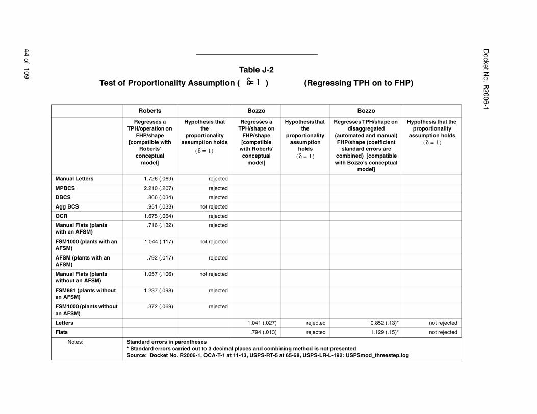
Docket N
o. R2006-1
44 of 109
n to FHP)
/shape on ated manual) efficient
ors are mpatible nceptual
]
Hypothesis that the proportionality
assumption holds
.852 (.13)* not rejected
.129 (.15)* not rejected
threestep.log
δ 1=( )
Table J-2
Test of Proportionality Assumption ( ) (Regressing TPH o
Roberts Bozzo Bozzo
Regresses a TPH/operation on
FHP/shape [compatible with
Roberts' conceptual
model]
Hypothesis that the
proportionality assumption holds
Regresses a TPH/shape on
FHP/shape [compatible
with Roberts' conceptual
model]
Hypothesis that the
proportionality assumption
holds
Regresses TPHdisaggreg
(automated andFHP/shape (co
standard errcombined) [cowith Bozzo's co
model
Manual Letters 1.726 (.069) rejected
MPBCS 2.210 (.207) rejected
DBCS .866 (.034) rejected
Agg BCS .951 (.033) not rejected
OCR 1.675 (.064) rejected
Manual Flats (plants with an AFSM)
.716 (.132) rejected
FSM1000 (plants with an AFSM)
1.044 (.117) not rejected
AFSM (plants with an AFSM)
.792 (.017) rejected
Manual Flats (plants without an AFSM)
1.057 (.106) not rejected
FSM881 (plants without an AFSM)
1.237 (.098) rejected
FSM1000 (plants without an AFSM)
.372 (.069) rejected
Letters 1.041 (.027) rejected 0
Flats .794 (.013) rejected 1
Notes: Standard errors in parentheses* Standard errors carried out to 3 decimal places and combining method is not presentedSource: Docket No. R2006-1, OCA-T-1 at 11-13, USPS-RT-5 at 65-68, USPS-LR-L-192: USPSmod_
δ 1=
δ 1=( )δ 1=( )
Appendix J
[117] In terms of hypothesis testing of the proportionality assumption, there may
not be a clear winner on this record. However, the Commission notes that to legitimize
his models, Dr. Bozzo needs to show that operation-level TPH is proportional to plant
level FHP, because his models use operation-level TPH, not plant-level TPH, as a proxy
for volume. If the proportionality assumption doesn’t hold at that level, Dr. Bozzo’s
models are mis-specified.
[118] Of more significance than the hypothesis testing that has been conducted on
this record is the fact that the proportionality assumption is violated by simply looking at
the ratio of TPH/FHP and seeing how it changes, both over time and across plants. See
Roberts March 2006, Tables 1 and 2.
b. Technical Issues
(1) Data Quality
[119] The Postal Service’s Management Operating Data System (MODS) records
work hours and piece handlings incurred in each mail processing operation in each mail
processing plant. Like most self-reporting systems, MODS generates a mountain of
observations at the level at which the data are first collected and reported. The obvious
downside to such a scheme is that the data set may be quite inaccurate, since the quality
controls exercised at the source are likely to be minimal. The MODS reports are also
susceptible to censorship and manipulation because the basic purpose of MODS is to
enable management to evaluate the performance of the Service’s mail processing
plants. See PRC Op. R2005-1, Appendix I, at 23 of 62.
[120] Since these data were first made the basis for econometric modeling of mail
processing cost variability, the Commission has consistently concluded that they are too
error ridden to produce estimates that are sufficiently free of bias to be relied upon for
ratemaking. See PRC Op. R97-1 ¶¶ 3040-3046; PRC Op. R2000-1 at 90, 97; PRC Op.
R2005-1, Appendix I, at 29-33, 37, 52.
45 of 109

Docket No. R2006-1
[121] Significance of error in the output variable. Measurements of the variables
that are to be used as explanatory terms in the estimated variability models must be error
free. The Commission has warned since Docket No. R97-1 that the consequences that
follow from using a sample that contains a substantial level of error can be severe.
When fit to the sample, the model’s estimated coefficients are likely to be biased and
inconsistent. “Biased” means that the estimated coefficients are expected to be different
from those of the true coefficients. “Inconsistent” means that the bias will remain even if
the sample is large. PRC Op. R97-1 ¶¶ 3041-3043.
[122] Measurement errors in an explanatory variable bias the estimated coefficient
on that variable toward zero if these errors are independent and identically distributed.21
The greater the variability in the measurement error, the greater the downward bias.
This is clear in the case of a model with a single explanatory variable, but in a
multi-variable model, there is a general tendency for the set of estimated coefficients to
collectively move toward zero.22 This effect is magnified when estimators are used that
difference the data, and thereby remove much of the cross-sectional variation in the
panel. This is true of all of the models proposed in this docket, all of which use fixed
effect estimators. See the relevant econometric literature summarized in 2006 Paper at
50.
[123] Significance of error in the work hours variable. The dependent variable in
the mail processing labor demand models under review is work hours in the sorting
operation, or the plant as a whole. These hours are calculated from clock rings in which
the worker is responsible for swiping a badge across the appropriate reader whenever
he enters or leaves a MODS operation. Employees are sometimes not sufficiently
motivated to ring in and out of an operation if changes in assignment are frequent or
21 When there are many bad observations present, the regression can present a description that mixes measurement of how the dependent variable is related to the explanatory variables in the correctly observed portion of the sample, and how the bad observations were generated in the erroneous portion of the sample. This reduces the apparent response of the dependent variable to the independent variable.
22 Robert S. Pindyck and Daniel L. Rubinfeld, Econometric Models and Econometric Forecasts, 2nd
ed, McGraw-Hill, 1981, at 177.
46 of 109

Appendix J
short term and their pay is not affected. Witness Neels demonstrates that misclocking is
common in the MODS data, as indicated by the observation of data collectors in the
overlapping IOCS system. UPS-T-1 at 15.
[124] If measurement error (misclocking) in the work hours variable has a zero
mean with a constant variance, is additive, and uncorrelated with the right-hand-side
explanatory variable, then the error is likely to be incorporated into the regression
disturbance term, resulting in an unbiased and consistent least-squares estimate of the
explanatory variable coefficient as long as the measurement error and the regression
disturbance term are uncorrelated.23 But if the measurement error is systematically
related to the dependent variable, then least-squares estimation can cause bias in the
estimate of the output coefficient.24 A systematic relationship between misclocking and
output might plausibly occur, for example, if work hours are underreported by workers
whose productivity is evaluated on that basis relative to other workers.
[125] Also, when there are many bad observations in the dependent variable,
there can be an increased probability of finding observations with outlying residuals,
which is likely to disproportionately affect the estimates. See PRC Op. R2005-1,
Appendix I at 36 of 62.
[126] Evidence of error in the MODS data. At the conclusion of Docket No. R97-1,
the Commission observed “[e]conometricians are accustomed to using data as they find
it, however the MODS data…are far below the common standard.” PRC Op. R97-1, ¶
3041. Nothing has been done in the ten intervening years to cause the Commission to
reconsider that observation.
[127] The nature and extent of the errors in the MODS piece handling data were
thoroughly documented in Docket Nos. R2000-1 and R2005-1, and again by witness
Neels in this docket. In Docket No. R97-1, a study of MODS data quality by the Postal
23 Pindyck and Rubinfeld, at 177.
24 Jeffrey M. Woolridge, Introductory Econometrics: A Modern Approach, South-Western College Publishing, 2000, at 293.
47 of 109

Docket No. R2006-1
Inspection Service was cited which concluded that there were large variances between
the piece handling figures contained in the MODS system and actual piece counts. See
Id., ¶ 3044. Most of this kind of error, however, is not extreme enough to be detected
without a special study like that conducted by the Inspection Service.
[128] Added to this implicit error are a wide variety of explicit error — error that is
so blatant that it is self identifying upon inspection. Errors of this kind abound in the
MODS data. They include hours or handlings with negative values, instances where
hours are positive and handlings are zero (or vice versa), instances where First Handled
Pieces are greater than Total Piece Handlings, and (for automated operations) instances
where Total Piece Handlings are greater than Total Pieces Fed. There are also
instances where the ratio of hours to handlings implies productivities that are either too
low or too high to reflect actual operating conditions. There are numerous “drop outs”
(periods when reporting of values intermittently ceases). The Postal Service does not
distinguish reporting drop outs from valid zero observations (those that indicate that a
relevant operation was temporarily shut down).
[129] MODS data are collected by shift, and rolled up by day, week, Accounting
Period, and Quarter. Errors that would be explicit by shift tend to be masked when rolled
up into a daily count. The masking increases with the level of aggregation. The degree
of masking can be considerable by the time that MODS data are rolled up into Quarters
— the level at which it is used in the various models under review in this docket.
[130] For MODS data compiled at the weekly level, the frequency of explicit errors
is quite high. Table J-3 and Table J-4 below were constructed by witness Neels. They
show the frequency of explicit errors in the observations for automated and for manual
operations.
[131] For automated operations, Table J-3 shows unrealistic productivities
(measured by Total Pieces Fed per hour) range from 34.5 percent of observations for the
AFSM 100 to 3.9 percent for the BCS incoming operation. Most automated operations
are mid-way between these frequencies. UPS-T-1 at 18.
48 of 109

Appendix J
[132] For manual operations, Table J-4 shows unrealistic productivities
(measured by Total Pieces Handled per hour) range from 10.7 percent for Manual
Letters to 54.2 percent for Manual Parcels. As many of the other manual operations are
near the maximum as are near the minimum of that range. UPS-T-1 at 20.
[133] The explicit errors in observed productivity are extraordinarily high for a
database to support valid econometric work. They reflect only one of the half-dozen
Table J-3Data Errors for Automated Cost Pools
Line LabelBCS
OutgoingBCS
Incoming OCRFSM 1000
AFSM 100
Total SPBS
1 Total records in Analysis Data set
10,304 10,304 10,304 10,304 10,304 10,304
2 Valid zeros: Count of records where operation was not present at plant, or plant was not reporting data to MODS system
1,521 1,250 2,335 3,902 6,045 4,207
3 Potentially Valid Records 8,783 9,054 7,969 6,402 4,259 9,097
4 Gaps in the Data 141(1.6%)
96(1.1%)
1(0.0%)
24(0.4%)
12(0.3%)
172(2.8%)
5 HRS, TPF, FHP or TPH < 0 512(5.8%)
194(2.1%)
44(0.6%)
41(0.6%)
8(0.2%)
12(0.2%)
6 HRS, TPF, or TPH=0 1,178(13.4%)
847(9.4%)
180(2.3%)
286(4.5%)
132(3.1%)
1,082(17.7%)
7 Record Fails Threshold or Productivity Screens at the Quarterly Level
257(2.9%)
104(1.1%)
189(2.4%)
197(3.1%)
578(13.6%)
65(1.1%)
8 TPH Fails Threshold or Productivity Check at the AP or Weekly Level
652(7.4%)
336(3.7%)
1,196(15.0%)
780(12.2%)
1,365(32.0%)
228(3.7%)
9 TPF Fails Threshold or Productivity Check at the AP or Weekly Level
726(8.3%)
354(3.9%)
1,120(14.1%)
840(13.1%)
1,469(34.5%)
226(3.7%)
10 FHP > TPH 1,946(22.2%)
1,279(14.1%)
3,063(38.4%)
1,155(18.0%)
1,529(35.9%)
910(14.9%)
11 FHP > TPF 1,252(14.3%)
1,150(12.7%)
1,110(13.9%)
779(12.2%)
882(20.7%)
634(10.4%)
12 TPH > TPF 16(0.2%)
27(0.3%)
3(0.0%)
41(0.6%)
67(1.6%)
129(2.1%)
Source: UPS-T1-Neels-WP-1 MODS Data/Data Errors/Output/Data Error Counts.xls (UPS-T-1, Table 4 at 18)
49 of 109

Docket No. R2006-1
categories of explicit error in the MODS data. Such rates of explicit error must be
regarded as symptomatic of a data measuring, recording, verifying, auditing, and
archiving process that is broken. The Commission agrees with Neels that “One must
wonder about the reliability of a data reporting system that produces obviously erroneous
results up to 30, 40, or as much as 50 percent of the time.” Id. at 26.
[134] Witness Bozzo argues that his screens are effective at removing explicit
error in the MODS data, and implies that the implicit errors that remain are not
significant. As evidence, he cites the results of a sensitivity check that he conducted,
using his preferred models. Witness Bozzo re-estimates his variability models using a
sample constructed by using threshold and productivity screens at the weekly and
accounting period level. He obtains a composite variability of 84 percent from his models
Table J-4Data Errors for Manual Cost Pools
Line LabelManual
FlatsManual Letters
Manual Parcels
Manual Priority Cancellations
1 Total records in Analysis Data Set 10,304 10,304 10,304 10,304 10,304
2 Valid zeros:Count of records where operation was not present at plant, or plant was not reporting data to MODS system
1,301 1,219 2,052 2,071 1,589
3 Potentially Valid Records 9,003 9,085 8,252 8,233 8,715
4 Gaps in the Data 65(0.7%)
32(0.4%)
100(1.2%)
203(2.5%)
33(0.4%)
5 HRS, FHP or TPH < 0 16(0.2%)
2(0.0%)
5(0.1%)
47(0.6%)
5(0.1%)
6 HRS or TPH = 0 120(1.3%)
104(1.1%)
1,310(15.9%)
967(11.7%)
212(2.4%)
7 Record Fails Threshold or Productivity Screens at the Quarterly Level
589(6.5%)
176(1.9%)
1,747(21.2%)
1,145(13.9%)
259(3.0%)
8 TPH Fails Threshold or Productivity Check at the AP or Weekly Level
2,106(23.4%)
971(10.7%)
4,470(54.2%)
3,500(42.5%)
1,052(12.1%)
9 FHP > TPH 32(0.4%)
24(0.3%)
41(0.5%)
113(1.4%)
0(0.0%)
Source: UPS-T1-Neels-WP-1 MODS Data/Data Errors/Output/Data Error Counts.xls (UPS-T-1, Table 5 at 20)
50 of 109

Appendix J
with strict screens compared to the composite variability of 86 percent that he obtains
from his model with quarterly screens. He concludes screening at the stricter level
[h]ad relatively little effect on most variabilities. Stricter screening does not serve to systematically increase or decrease the variabilities. The exception is that the IV models for manual parcels and manual Priority show increases in the point estimates but also rapidly increasing standard errors.
USPS-T-12 at 97.
[135] Bozzo neglected to evaluate what his results show when manual priority
variability is left in. Using weekly screens causes manual priority variability to triple to
228, manual parcel to rise from 80 to 97 percent, and cancellation to rise from 50 to 59
percent. The composite variability rises from 85 to 93 percent.
[136] When Bozzo moved from quarterly screens to weekly screens, he
dramatically reduced the size of the samples that he used, as shown in Table J-5 below.
The operations whose variabilities were most affected by stricter screens are generally
the same ones whose experienced the largest reduction in sample size. Whether the
substantial changes in variability estimates were caused directly by eliminating
erroneous observations or indirectly through changes in the composition of the sample is
not known, but the ultimate cause of the changes in variability estimates is the need to
mitigate errors in the output variable. Bozzo’s sensitivity check strengthens the
Commission’s conclusions that screening for explicit error does not eliminate
errors-in-variables bias, and that quarterly screens do not catch all of the errors that
matter.
[137] Analyzing the tables constructed by witness Neels reinforces the conclusion
that the level at which one inspects the MODS data has a substantial effect on the
frequency at which explicit errors appear. Neels shows that when one moves from the
quarterly level to the weekly level, the frequency with which obviously unrealistic
productivities are recorded rises sunstantially for automated operations but rises
51 of 109

Docket No. R2006-1
dramatically for manual operations. See UPS-T-1 at 18 (Table 4, rows 7-9), and at 20
(Table 5, Rows 7-8).
[138] When witness Neels developed his plant-level model of mail processing
variability, he performed a similar sensitivity analysis. Witness Neels argues mail
processing labor variability should be modeled for the plant as a whole, rather than at the
level of individual operations or sets of operations within the plant. To be reliable, a
plant-level model requires error-free data for the entire plant.
[139] In preparing a database free of explicit error for the entire plant, Neels found
that the cumulative effect of screening out explicit error at the weekly level is dramatic.
As can be seen from Table J-6 above, only 920 out of 10,304 records (about nine
percent) were valid for the entire plant. At the quarterly level, the results of screening are
much less severe. At the quarterly level, 2,155 out of 10,304 records (about 21 percent)
Table J-5
Changes in Variabilities Resulting from Stricter Quality Standards
Cost PoolRecommended Variabilities –
Quarterly ScreensWeekly Level
ScreensPercent
Difference
BCS Outgoing 1.06 1.09 3%
BCS Incoming 0.82 0.81 -1%
OCR 0.78 0.68 -13%
FSM/1000 0.72 0.70 -3%
AFSM100 0.99 0.90 -9%
SPBS 0.87 0.84 -3%
Manual Flats 0.94 0.89 -5%
Manual Letters 0.89 0.87 -2%
Manual Parcels 0.80 0.97 21%
Manual Priority 0.75 2.28 204%
Cancellations 0.50 0.59 18%
True Composite 0.85 0.93 9%
Composite excluding Manual Priority
0.86 0.84 -2%
Source: UPS-T-1 Table 8 at page 25 (USPS-T-12, Table 26)
52 of 109

Appendix J
were valid for the entire plant. The difference in screening level produced significantly
different variability estimates. Neels’ model, using data screened at the weekly level,
produced an aggregate plant variability of 114 percent. At the quarterly level, estimated
variability was 103 percent.
[140] The sensitivity analyses performed by Bozzo and Neels result in dramatic
reductions in the size of their usable samples, and significant differences in their
variability estimates. These results strongly imply that enough explicit error remains in
the data when screened at the quarterly level to make the resulting estimates unreliable
for ratemaking.
Table J-6
Sample Size Reduction for Plant Level Models
Line No. Description Flats Letters Parcels Priority Models
1 Potentially Valid Records 10,304 10,304 10,304 10,304 10,304
2 Gaps 10,203 10,110 10,035 10,101 10,271
3 HRS, TPF, FHP, or TPH < 0 10,138 9,390 10,018 10,054 10,266
4 HRS, TPF, or TPH = 0 9,638 7,729 7,906 9,099 10,055
5 Record Fails Threshold or Productivity Screens at the Quarterly Level
8,461 7,380 6,316 8,024 9,848
6 TPH Fails Threshold or Productivity Check at the AP or Weekly Level
6,457 6,298 4,960 6,583 9,213
Strict Sample Loose Sample
7 Records that are valid across all shapes
1,978 3,297
8 Records for plants not in operation 816 816
9 Records with no missing variables 1,162 2,481
10 Records for plants with more than one record (final sample size)
920 2,155
Source: UPS-T-1 Table 20 at 52.
53 of 109

Docket No. R2006-1
[141] Problems with the capital data. Witness Roberts has noted that when new
mail processing machines are deployed in a plant, there is a time lag between MODS
labor and output data recorded in an operation and the capital data recorded in the
Personal Property Asset Master (PPAM) and Property and Equipment Accounting
System (PEAS) OCA-T-1 at 20. The MODS data will begin to log labor hours and
volume (TPF, FHP) for the new machines several time periods before it is recorded as
capital in the capital measures coming from the PPAM/PEAS property reporting systems.
[142] Two workarounds that have been used by witnesses Roberts and Bozzo are
described in OCA-T-1 at 20. One deletes a plant’s data for the first year in which the
AFSM is operating in the plant. Roberts contends that this does not really fix the
problem. If the pattern of equipment deployment reflects errors in data reporting, he
says, then whenever there is an increase in investment in the plant, the capital variables
will not accurately measure the change in the right time periods. Bozzo shifts the capital
variables backward in time, but Roberts argues that this is not a substitute for getting the
information in the two data systems (MODS and PPAM/PEAS) correctly synched.
[143] The effects that the mismatch between hours and piece handling data and
capital equipment deployment has on the size of the estimated capital coefficients and
their significance are largely unknown. Witness Bozzo uses an alternative capital series
based on “quarterly” updating, USPS-T-12 at 100-101. Comparing the results using the
annual updates with those obtained using the quarterly updates, he finds relatively little
difference. Id. at 101.
[144] Witness Bozzo also found very little difference when estimating log-linear
models using the constructed capital measures by witness Roberts’ aggregated constant
dollar investment expenditure capital measures (FSM, DBCS, MPBCS, SPBS, other)
and his own (aggregated investment expenditure capital measure across plants using
constructed plant-level shares). Id. at 92.
[145] Witness Roberts argues that the Postal Service’s models are misspecified
because they aggregate capital from several operations and include it as an explanatory
variable in all the labor demand equations. He says that this is not consistent with
54 of 109

Appendix J
Bozzo’s assumption that the production stages are separable. Nor does it allow the
capital in one operation to be substituted for labor in another related operation without
being interpreted as a change in output. See 2006 Paper at 19, 24-25, and 2002 Paper
at 11-12.
[146] Witness Bozzo recognizes that his estimated capital elasticities are small,
often statistically insignificant, and mixed in arithmetic sign. USPS-T-12 at 81. He says
that these results are consistent with his assumption that “the main way in which capital
affects labor input is by providing capacity in higher productivity (automated) operations,
rather than by making specific (existing) mail processing operations more productive.” Id.
This, however, would only be true in the very short run. It is unlikely to be true over a rate
cycle.
[147] A Hausman or comparable test of the exogeneity of capital variables
constructed from the PPAM/PEAS system would be potentially valuable in helping to
assess the potential bias from measurement error that appears to infect these
variables.25.
(2) Correcting for errors in the MODS data.
[148] Most of the sources of the implicit and explicit errors in the MODS data
described above are not known. Two potential sources of error are acknowledged as
likely, but their relative contribution to the errors described above is not known.
Misclocked work hours contribute to the errors described above because they are the
denominator of the ratio of piece handlings to work hours in the manual sorting
operations. The other acknowledged source of error is the set of factors used by the
Postal Service to convert pounds of mail to pieces. When it is not practical to count mail,
the Postal Service weighs it and infers the number of pieces from national standard
25 In order to implement this test, a set of instruments would be needed that predicts the level of capital at specific plants. This is an example of the need for site-specific data in order to identify valid instruments and make progress on the econometric estimation of mail processing variability
55 of 109

Docket No. R2006-1
conversion factors. Conversion factors are inaccurate because they are not plant
specific, and many years go by between updates. Conversion factors are needed to
compute FHP in each operation. They are also the basis of TPH counts for the manual
operations. Both Drs. Bozzo and Roberts treat error from conversion factors as the
major source of error in FHP.
[149] Roberts demonstrated that errors arising from conversion factors are
potentially large. He estimates that the use of obsolete conversion factors prior to 1999
had led the FHP count of letters to be overestimated by 18 percent, and of flats to be
overestimated by 11 percent. See Roberts 2002 at 49. Drs. Bozzo, Roberts, and Neels
acknowledge that the conversion factors used to estimate FHP counts are potentially a
source of substantial measurement error that risks errors-in-variables bias, and all have
turned to the use of Instrumental Variables estimators as a way of mitigating that risk.26
[150] The need for instruments. Instrumental variables are commonly used in
econometric modeling to overcome the endogeneity of a regressor (the correlation of a
regressor with the regression error term). Instruments are variables that partly cause the
endogenous regressor. This causal relationship can be used to recover an estimate of
the conditional mean of the endogenous regressor.27
[151] As explained in the Commission’s summary of Roberts’ research,
instrumental variables is a method used to get consistent estimates of an economic
relationship when the “causing” variable (in this context pieces or piece handlings)
transmits more than the cause to the outcome variable. For example, FHP transmits the
effect of both volume variation and measurement error to work hours.
26 Bozzo is so confident that the use of Instrumental Variables solves the problem of errors-in-variables bias that he regards screening of all data that is identifiably erroneous as unnecessary. USPS-RT-5 at 27.
27 A common method for consistently estimating the parameters of a linear model with a right-hand-side endogenous variable is called Two-Stage Least Squares. The first stage of the analysis takes the endogenous variable in the regression of interest and regresses it on the remaining right-side variables in the equation of interest and the instrumental variables. The second stage of the analysis inserts the fitted value of the dependent variable from the first-stage back into the regression of interest and computes the least squares estimates of this regression.
56 of 109
Appendix J
[152] All of the econometric witnesses agree that imprecise weight-to-pieces
conversion factors measure FHP with error. To the extent that it is imprecisely
measured, variation in FHP transmits both the effect of variations in volume and the
effect of measurement error to work hours. As explained in the previous section, mixing
these effects is likely to bias the estimated response of work hours to volume downward.
[153] Roberts acknowledges that this is especially true for the Fixed Effect models
under review. Fixed Effects models remove much of the variation in the volume variable
that is available for modeling. This magnifies measurement error relative to the volume
variation that remains. Roberts March 2006 at 50.
[154] Conditions for valid instruments. The conditions that instruments must meet
in order to be valid, however, are quite demanding. The basic idea of Instrumental
Variables regressions is to find an instrument that causes or explains only the variation in
the volume variable that is “true” volume variation, but is independent of the variation in
the volume variable that represents other things — such as measurement error in that
variable.
[155] As explained in Appendix L, these are rigorous requirements. In order to be
valid, the instrument must be exogenous to the underlying model, that is, it must affect
work hours only through its effect on the endogenous “volume” variable (FHP). It must
not affect work hours directly.28 (If the instrument affected work hours directly, it would
belong in the set of control variables in the regression of interest). In addition, the
instrument must be “relevant,” that is, it must cause or verifiably explain the portion of the
variation in the endogenous “volume” variable that is not caused by omitted variables or
by measurement error.29 If it explains any of the erroneously measured part (if a factor
that makes the measure of the “volume” variable erroneous also makes the measure of
the instrument erroneous) the instrument will transmit the error in the “volume” variable
through to work hours. This would defeat the instrument’s purpose.
28 Holland, P.W., “Causal Inference, Path Analysis and Recursive Structural Equation Models,” Sociological Methodology, 18, 449-84, Angrist, J. and Imbens, G. “Estimation of Average Causal Effects,” Journal of the American Statistical Society, 91, 444-72.
57 of 109

Docket No. R2006-1
[156] As explained in Appendix L, it is impossible to demonstrate that an
instrument is valid through a statistical test.30 To be credible, an assertion that an
instrument actually eliminates endogeneity, such as that caused by measurement error,
needs a convincing theory that identifies the cause of the endogeneity, and a convincing
theory that explains why the instrument is independent of that cause. In addition, the
instrument must capture the “true” variation in the “volume” variable, not just coincidental
correlation. This also requires a sound theory as to why the instrument is a partial cause
of the “volume” variable, rather than simply responding to common factors that cause
them both.
[157] Relevance of the instruments under review. Although all three researchers
have employed instrumental variables in their models, and their instruments differ. See
Table J-7 below), Roberts has shouldered most of the burden of identifying plausible
instruments, providing a theoretical justification for their use, and testing their validity.
The Commission’s conclusions with respect to the validity of the instruments that he uses
generally will apply to the instruments used by the others.
[158] To illustrate, in Roberts September 2006, Roberts uses as instruments for
FHP/letters: FHP flats/incoming, FHP/flats/outgoing, quarterly dummy variables, and the
number of destinating letters, flats, and parcels in a plant’s service area. He asserts that:
[a]ny exogenous source in the demand for mail services will lead to fluctuations in the FHP variables that are not correlated with the error term and, as a result, will be useful as an instrumental variable. In short,
29 Angrist, J. and Kreuger, A., Instrumental Variables and the Search for Identification: From Supply and Demand to Natural Experiments, Journal of Economic Perspectives — 15, No. 4 (Fall 2001), at 73. The causal effect must run from the instrument to the endogenous “volume” variable, not the other way. If some intervening force should change the value of the “volume” variable, it must not affect the instrument. See Rubin, D.B., Statistics and Causal Inference: Comment: Which Ifs Have Causal Answers,” Journal of the American Statistical Association, 81, 961-962 (1986).
30 It is possible, of course, to increase one’s confidence that an instrument is relevant by testing the significance of the instrument’s coefficient in the first stage of a Two Stage Least Squares regression and obtaining a high ‘”t” value. That will indicate the strength of the correlation of the instrument with the endogenous explanatory variable, but it will not indicate whether the correlation is theoretically meaningful, or merely coincidence.
58 of 109
Appendix J
variables that measure fluctuations in the demand for mail services will be good instrumental variables (IVs) because they will be correlated with FHP but not correlated with the technology shocks or output measurement errors captured by the error terms.
OCA-T-1 at 28.
[159] These criteria are broad, vague, and conclusory. By themselves, they do not
have the theoretical rigor required to provide reasonable assurance that variables that
meet them would be valid instruments.
[160] Roberts is a bit more specific with respect to why FHP/flats is a valid
instrument for FHP/letters. He asserts that FHP/flats
reflect variation in the demand for mail services that can result from differences in the mix of business and household mailers in the plant’s service areas, differences in population and its growth over time, and other sources of differences in demand across plants.
Id. FHP/flats is much like true RPW flat volume. The volume of flats that arives at a plant
will certainly be a function of the mix of mailers, population trends, and other factors in
the plant’s service area, just as the volume of letters that arrives at a plant will be a
function of these factors. It is not enough, however, that the level of FHP/flats entering a
plant and the level of FHP/letters entering a plant are both a function of local business
conditions and consumer wealth characteristics. To be valid, an instrument for
FHP/letters must not just be correlated with the FHP/letters, it must partially cause
variation in FHP/letters.
[161] It is not plausible to characterize variation in FHP/flats as a source of
variation in FHP/letters. The plausible sources of variation in FHP/letters include such
things as the profile of local business mailers (utility billers, credit card issuers, etc.), the
disposable income of local recipients of mail, the pace of local household formation, the
price and availability of competing forms of communication and advertising, etc. The
proximity of other postal facilities, and their capacity and function are also plausible
causes of the amount and kind of mail that a plant receives. These are much the same
59 of 109

Docket No. R2006-1
Table J-7Instrumental Variables Compared
Level of Analysis Analyst
Dependent variable
Endogenous explanatory
variableSource of
endogeneityInstrument(s)
used
Operations Level Manual
Letters
Bozzo Letter Hours TPH Conversion Factor
FHPfsm881,FHPfsm1000, FHPafsm100,
TPHmanualflats, DestinatingLetterVol
Operations Level Manual
Flats
Bozzo Flats Hours TPH Conversion Factor
FHPocr, FHPmpbcs, FHPdbcs,
TPHmanualletter, DestinatingFlatsVol
Operations Level Priority
Bozzo Priority Hours
TPH Conversion Factor
FHPocr, FHPmpbcs, FHPdbcs, FHPfsm881,
FHPfsm1000, FHPafsm100,
DestinatingPriorityVol
Operations Level Parcels
Bozzo Parcel Hours TPH Conversion Factor
FHPocr, FHPmpbcs, FHPdbcs, FHPfsm881,
FHPfsm1000, FHPafsm100,
DestinatingParcelsVol
Operations Level
Cancellation
Bozzo Cancellation Hours
TPH Conversion Factor
FHPocr, FHPmpbcs, FHPdbcs,
DestinatingLetterVol
Plant Level Shape-based
Letters
Roberts Letter Hours FHP Conversion Factor
FHPflats outgoing, FHPflats incoming,
DestinatingLetterVol, DestinatingFlatsVol,
DestinatingParcelsVol
Plant Level Shape-based
Flats
Roberts Flats Hours FHP Conversion Factor
FHPletters outgoing, FHPletters incoming, DestinatingLetterVol, DestinatingFlatsVol,
DestinatingParcelsVol
Plant Level Letters,
Flats, and Parcels
Neels Total Plant Hours
FHP Measurement Error
TPHletters, TPHflats, TPHparcels,
DestinatingLettersVol, DestinatingFlatsVol,
DestinatingParcelsVol
Source: Docket No. R2006-1, USPS-T-12, USPS-LR-L-56; OCA-T-1, OCA-LR-L-2; UPS-T-1, UPS-Neels_WP-1
60 of 109

Appendix J
Table J-7 (Continued)
Instrumental Variables Compared (part 2)
Is the instrument correlated with
measurement error in the endogenous output variable?a
Theory for why the instrument causes
the endogenous explanatory variable
Is the endogenous explanatory variable and the instrument
likely to be caused by the same
phenomena?
Will the instrument directly affect the
dependent variable?
Probably None Yes No
Probably None Yes No
Probably None Yes No
Probably None Yes No
Probably None Yes No
Probably Correlation Explanation
Yes No
Probably Correlation Explanation
Yes No
Probably None Yes Yes
a/ Where destinating volume is used as an instrument it is not likely to be correlated with measurement error in the endogenous output variable.
61 of 109

Docket No. R2006-1
as the plausible sources of variation in FHP/flats. This would make FHP/flats a spurious
instrument for FHP/letters. 31 FHP/flats cannot be used to extract the “relevant” portion of
the variation in FHP letters that is free of confounding effects. It can only mimic
FHP/letters. If one were to imagine an array of intervening forces that could affect
FHP/letters (e.g., a local recession, a surge of home construction) most of them would be
expected to affect FHP/flats as well. This means that FHP/flats is not a well-defined
instrument for FHP/letters.32 Instead of FHP/flats, plausibly valid instruments for
FHP/letters would by the underlying causes of variation in both. These would include
measures of the economic and business conditions in the service area of a plant
described above.
[162] Roberts included quarterly dummy variables in what was initially his
preferred model. P values from a test of the joint significance of Roberts’ group of
instruments showed that quarterly dummies made a large contribution to explaining
variation in FHP/letters in the first stage of a Two Stage Least Squares estimate.
OCA-T-1, Table 2 at 32. As theoretical support for using quarterly dummies as
instruments, Roberts observes that the volume of FHP/letters and FHP flats fluctuates
markedly by quarter. Id., Figure 1, at 30. He argues that
31 An intuitive example of a spurious correlation would be sales of ice cream and sales of soda by local outdoor vendors. Both are likely to rise strongly in summer, as outdoor recreation increases. A statistical test would reflect the strong correlation. But sales of ice cream do not logically cause sales of soda. The true cause is the warm weather, which encourages both. Ice cream sales would be a spurious instrument to use to predict sales of soda, despite their close correlation. A true causal relationship likely exists between the quantity of chips and soda sold by outdoor vendors. Warm weather increases outdoor recreation, causing outdoor sales of both chips and soda to rise. But, because salty chips increase thirst, they independently encourage sales of soda. This correlation would be meaningful because there is a plausible causal theory to explain the correlation. For this reason, sales of chips (in an earlier period) should be a valid instrument for sales of soda.
In the mail processing context, the relationship between FHP flats and FHP letters is analogous to the relationship between sales of soda and sales of ice cream in the above example. They are correlated, but the correlation is not meaningful. They are spurious instruments for each other. The local business cycle is analogous to the weather in the above example. It is a plausible cause of variation in both FHP letters and FHP flats, and might make a theoretically relevant instrument for either.
32 See Rubin, D.B., Statistics and Causal Inference: Comment: Which Ifs Have Causal Answers,” Journal of the American Statistical Association, 81, 961-962 (1986).
62 of 109
Appendix J
[t]his quarterly variation is due to the actions of mailers and is a nice source of exogenous variation in FHP. The quarterly dummy variables satisfy the requirements for good IVs.
Id. at 29. [163] While the seasonal variation of FHP/letters is pronounced, and is
mailer-induced, quarterly dummies do not capture that seasonal variation cleanly.
Quarterly dummies, therefore are not “exogenous” in the sense required to be a valid
instrument. To be exogenous, an instrument for FHP/letters should not have a direct
effect on work hours. While quarterly dummies will capture the effect that seasonality
has on the quantity of FHP/letters, they are also likely to capture such things as seasonal
shifts in the composition of the workforce (such as the percent that is casual labor) and
seasonal changes in the composition of the mail (such as the percent of letters that are
single-piece and non-machinable). The latter two factors can affect work hours directly.
This violates the condition that instruments not have a direct effect on the dependent
variable in the equation of interest.33
[164] Roberts’ group of instrumental variables includes the number of destinating
letters, flats, and parcels in a plant’s service area. As justification for using them as
instruments for FHP/letters, Roberts notes that they
are measured externally to the MODS data using ODIS…and are potentially useful measures of differences in mail demand across plants and time periods.
OCA-T-1 at 29.
[165] Roberts does not actually discuss the theoretical relationship between
destinating volume for each shape in a plant’s service area and FHP/letters in a plant.
The theoretical relationship between FHP/letters and destinating flats, and FHP/letters
and destinating parcels, however, is much the same as the relationship between
33 Wooldridge, J., Introductory Economics: A Modern Approach, South Western College Publishing (2000) at 463.
63 of 109

Docket No. R2006-1
FHP/letters and FHP/flats. It is not plausible to characterize variation in FHP/letters as a
“function of,” “caused by,” “explained by,” or “encouraged by” either destinating flat
volume or destinating parcel volume. These variables, however, all have plausible
common sources--such things as the business cycle in the plant’s service area, the mix
of local businesses (e.g., catalogue mailers, fulfillment companies), disposable income of
local recipients of mail, etc. Because the plausible sources of variation in destinating flat
volume and destinating parcel volume are shared with FHP/letters, they should be
considered to be spurious instruments for FHP/letters. Neither destinating flats nor
destinating letters could be used to extract just the “relevant” portion of the variation in
FHP/letters free of confounding, non-volume effects. At best, they might mimic the
variation observed in FHP/letters because of their common sources. That their variation
reflects common sources is also seen when one hypothesizes intervening forces that
could affect FHP/letters (e.g., a local business recession, a surge of home construction).
These interventions are as likely to affect destinating flat volume and destinating parcel
volume as destinating letters. For these reasons, destinating flats and destinating
parcels are not well-defined instruments for FHP/letters.
[166] Of all the instruments employed by Roberts, destinating letter volume
appears to meet the theoretical requirements of a valid instrument for FHP/letters.
Destinating letter volume can be viewed as the immediate cause of
FHP/letters/incoming, since it is precisely what generates FHP/letters/incoming.
Destinating letter volume is also the immediate cause of that portion of
FHP/letters/outgoing that is made up of local, turnaround letters. FHP/letters can be
considered a partial function of destinating letter volume. Destinating letter volume is
exogenous, since it will not affect work hours in a letter sorting operation directly, but only
as it causes FHP/letters to vary.
[167] In the context of Roberts models, the problem with using destinating letter
volume as an instrument for removing the endogeneity of FHP/letters is empirical, rather
than theoretical. Since incoming letter processing accounts for over two-thirds of the
cost of all letter processing, one would expect the correlation between FHP/letters in a
64 of 109

Appendix J
plant and destination letter volume to be very high. Roberts, however, characterizes his
destinating volume instruments as not very significant in estimating “true” variation in
FHP/letters, as the P values presented in OCA-T-1, Table 2, confirm. By themselves,
destinating letters would constitute weak instruments. In the context of Two Stage Least
Squares estimation, weak instruments run the risk of adding bias to the estimated
results. Of the instruments in the group that Roberts used, destinating letter volume is
the only instrument that can be shown to be theoretically relevant to FHP/letters.
[168] In contrast to Roberts, Bozzo’s underlying model of labor demand
variability defines output at the operation level. It estimates the response of work hours
within an operation to variations in piece handlings (TPH) within that operation. He
believes that only the manual and cancellation operations risk bias from measurement
error. He also believes that TPH in an operation is exogenous, since he theorizes that
each sorting operation is autonomous and unaffected by the level of work performed in
other operations. Docket No. R2005-1, USPS-T-12 at 26-27.
[169] As an instrument for TPH in a given operation, Bozzo uses FHP for
aggregated sorting operations of the opposite shape. A second instrument is destinating
volume of the opposite shape in the plant’s service area. The first instrument for
TPH/letters, therefore, would be an aggregation of FHP/manual flats, FHP/FSM1000,
and FHP/AFSM 100. The second instrument would be the volume of destinating flats in
the plant’s service area.
[170] Bozzo asserts that Roberts has established the theoretical relevance of
FHP of the opposite shape as an instrument for operation-level TPH. (He asserts, as
well, that Roberts has established the theoretical grounds for believing that
measurement error in FHP is independent of the measurement error in TPH.) Bozzo
adds only that “[t]he desired properties for an instrumental variable are correlation with
the ‘true’ regressor and independence from the observed regressor’s measurement
error.” Id. at 26.
[171] For the reasons explained above, the Commission has concluded that while
FHP of one shape may be correlated with FHP of a different shape, it is not plausibly a
65 of 109

Docket No. R2006-1
function of, or caused by, FHP of a different shape. Because the correlation stems from
common latent causes, FHP of a different shape is a spurious instrument. This applies
to Bozzo’s TPH variable all the more, because it is an operation-level rather than a
plant-level variable. It is difficult to view variation in plant-level FHP flats as a significant
source of variation in TPH for the Manual Letter operation. Taking this view should be
especially difficult for Bozzo, who theorizes that each sorting operation is unaffected by
the level of activity in other operations in the plant. The same analysis applies to
Bozzo’s use of destinating flat volume as an instrument for TPH/letters.
[172] Neels tested the relevance of Bozzo’s instruments. While a first-stage F
statistic testing the incremental explanatory power of the instruments shows that they are
jointly significant, Neels concludes from partial R-square statistics that the instruments
add little explanatory power to the first stage regression. Neels notes that use of weak
instruments raises the risk of biased estimates. UPS-T-1 at 29-30.
[173] Bozzo dismisses Neels’ assertion that his instruments are weak and
arbitrary. He argues that it is not based on a benchmark or critical value that is accepted
in the economic literature. USPS-RT-5 at 33-34. Neels’ criterion for concluding that
Bozzo’s instruments are weak and arbitrary is subjective. It leaves the technical issue of
the strength of Bozzo’s instruments unresolved. However, this issue is immaterial.
Whether or not his instruments are weak, the Commission has concluded that Bozzo’s
instruments lack a theory that would make the correlation meaningful for estimating a
causal relationship between hours and volume.
[174] As described earlier, Neels develops his own model of labor demand
variability which estimates the response of work hours for the entire plant to changes in
plant-level FHP for letters, flats, and parcels. It reflects his theory that labor demand
reflects economies of scope in mail processing, consisting of adjustments to volume that
are made within operations, across operations and across shapestreams. As a
consequence many more relationships would qualify as endogenous under the Neels
model than under the other models under review.
66 of 109

Appendix J
[175] As instruments for his FHP/shape output variables, Neels uses TPH counts
by shape, and destinating volumes by plant, by shape. He states that these instruments
pass tests of relevance and validity, but he does not offer any theoretical ground for their
use. UPS-T-1 at 52.
[176] The reason that the MODS system tracks FHP is that it provides the
manager a means of projecting workload and work hours in the plant that will result from
the amount and kind of FHP arriving at the plant. The manager does this by calculating
downflow densities based on experience that estimate the propensity of FHP with given
shape and processing characteristics to generate an expected count of TPH in various
operations.
[177] Using TPH as an instrument for FHP of a corresponding shape is putting the
cart before the horse — effect before cause. While it is quite plausible to view variation
in FHP as a source of variation in TPH, it is not plausible to view variation in TPH as a
source of variation in FHP, whether at the shape level or the plant level. Roberts has
made the argument that FHP is exogenous at the plant level because it results almost
entirely from the habits of mailers. But there is not much room to argue that TPH is
exogenous at the plant level. TPH depends on the amount of equipment in the plant,
and the sophistication of the technology that it embodies — all of which are the result of
discretionary decisions by management made (at least in part) in response to changes in
volume over a rate cycle.
[178] TPH fails a number of the tests of theoretical relevance for an instrument
that are found in the academic literature summarized earlier. TPH will not affect work
hours in the plant through its effect on the endogenous FHP variable, since it doesn’t
have an effect on FHP. It will affect work hours directly because it depends on
discretionary choices of what technology will be applied to the workload imposed by mail
arriving at the plant. This violates a basic condition for a valid instrument, as explained
earlier. TPH does not extract only the exogenous portion of the variability in FHP
because it transmits its own endogenous effects to work hours. Almost any intervention
that could be hypothesized that would affect FHP in the plant (e.g., a downcycle in the
67 of 109

Docket No. R2006-1
local business climate) would affect TPH as well, which violates another condition for a
valid instrument, as explained earlier. Most of the sources of variation in FHP (e.g., the
business climate and consumption patterns in the area served by the plant) are sources
of variation in TPH. Consequently, the common sources are the legitimate candidates as
instruments for FHP.
[179] RPW volumes are system-level volumes. Variations in system-level
volumes by shape would certainly be the dominant source of variation in FHP by shape
at the plant level. As a theoretical matter, these variables would appear to meet all of the
conditions required of relevant instruments that TPH fails. How relevant they are is an
empirical matter. Neels’ workpapers contain tests that show that they are statistically
relevant, but Neels did not report or comment on these results. See Workpapers,
UPS-Neels-WP-1, 3.5 Plant Level Model.
[180] Exogeneity of the instruments under review. In resorting to the use of the
Instrumental Variables estimation technique, the main motive of all three researchers
was to overcome the risk of biased estimates from errors in measuring the output
variable. Drs. Bozzo and Roberts assume that conversion factors are the dominant
source of measurement error in the output variable. When output cannot be counted, it
must be inferred by weighing the mail and using a conversion factor to infer the number
of pieces. FHP counts are based on this process, as is the major portion of TPH in
manual operations.34
[181] Using instruments to overcome measurement error in the endogenous
output variable (FHP or TPH) is based on the idea that a variable can be found that will
extract that portion of the variation in FHP that is independent of measurement error (or
any other source of non-volume variation). It is not necessary that the instrument itself
by free of error, just that its error be independent of the error in the FHP shapestream of
interest. Roberts 2002 at 54.
34 TPH in manual operations consists of First Handling Pieces (FHP) and Subsequent Handling Pieces (SHP).
68 of 109

Appendix J
[182] Noting that different conversion factors are used for different shapes,
Roberts reasons that FHP of a different shape will be free of the predominant source of
measurement error in FHP of the same shape. The assumption that the error in the
instrument is uncorrelated with the error in FHP cannot be proven through statistical
tests. Statistical tests can only indicate that this requirement is not met by particular
instruments when they are tested. Therefore, a convincing theory that explains why
variation in the instrument can be assumed to be independent of error in FHP/shape is
needed to be assured that use of the instrument will lead to reliable estimates.
[183] Conversion error. The fact that different weight-to-piece conversion factors
are used for different shapes might not be sufficient to ensure that they are independent.
Roberts concluded that obsolete conversion factors used prior to 1999 had caused letter
FHP to be overestimated by 18 percent and flat FHP to be overestimated by 11 percent,
reflecting a shared trend toward heavier pieces over time for both shapes. If the average
weight per piece for mail changes in the same direction over time, or by season,
conversion error could be correlated across shapes, even where the conversion factors
are shape-specific.
[184] Neels demonstrated that the average weight per piece changes substantially
over time for classes of mail. Tr. 23/8527. This implies that it changes substantially over
time for shapes of mail as well. Witness Oronzio observes that one reason that FHP
data is not trusted by plant managers is that the composition of the mail changes by
season. He remarks that even humid weather can alter the weight of the mail enough to
induce conversion error. USPS-RT-15 at 12.
[185] Systematic changes in weight per piece could cause corresponding changes
in conversion error and the work hours required to process mail. (The ounce/rates and
breakpoints common in postal rate schedules, in part, reflect the productivity of the
equipment that can be used to process mail of certain weight characteristics). There
appears to be a significant risk that conversion error is correlated with work hours in the
manner described. Figures J -1 through -3 below show a pronounced quarterly variation
69 of 109

Docket No. R2006-1
in average weight per piece for letters, for flats, and for parcels. This provides grounds
for skepticism that opposite shape FHP is an exogenous instrument.
[186] Other sources of measurement error. Even if conversion error in FHP of one
shape were truly independent of conversion error in FHP of other shapes, there are
sources of significant measurement error in MODS output data that are not related to
conversion whose effect is probably common to all shapes, and, therefore, correlated.
70 of 109

Appendix J
Figure J-1
Figure J-2
Figure J-3
LE TTE RS (QUA RTE RLY )
0.5
0.52
0.54
0.56
0.58
0.6
0.62
0.64
0.66
0.68
0.7
03Q
1
03Q
2
03Q
3
03Q
4
04Q
1
04Q
2
04Q
3
04Q
4
05Q
1
05Q
2
05Q
3
05Q
4
06Q
1
06Q
2
06Q
3
06Q
4
07Q
1
Y ear and Quarter
WE
IGH
T/P
IEC
E (
ounc
es)
FLATS (QUARTERLY)
4
4.05
4.1
4.15
4.2
4.254.3
4.35
4.4
03Q
1
03Q
2
03Q
3
03Q
4
04Q
1
04Q
2
04Q
3
04Q
4
05Q
1
05Q
2
05Q
3
05Q
4
06Q
1
06Q
2
06Q
3
06Q
4
07Q
1
Year and Quarter
WE
IGH
T/P
IEC
E (
ounc
es)
PARCEL (QUARTERLY)
20
25
30
35
40
03Q
1
03Q
2
03Q
3
03Q
4
04Q
1
04Q
2
04Q
3
04Q
4
05Q
1
05Q
2
05Q
3
05Q
4
06Q
1
06Q
2
06Q
3
06Q
4
07Q
1
Year and Quarter
WE
IGH
T/P
IEC
E (
ounc
es)
71 of 109

Docket No. R2006-1
[187] Kinds of measurement error that the witnesses seem not to have considered
when selecting instruments for FHP are the array of gross errors in the data — the
negative FHP counts, implausibly high or low productivity values, the pairing of zero
hours with positive FHP and vice versa, and the discontinuities in the data that are
treated as true zeros. The sources of these errors are likely to be common to all shapes
of mail. If these errors are essentially failures to collect the data, to record them by the
prescribed procedures, or to audit the data either at the source, or after aggregation,
such failures are most likely to be the result of the administrative problems that are
known to plague self-reporting data systems from which productivity can be inferred.
[188] Errors in self-reported productivity data that can give rise to the kind of
obvious errors that are common in the MODS data reflect a number of possible causes.
For example, they may reflect a manager’s decision to devote limited staff resources to
matters considered more urgent than routine data collection. The tension that exists
between allocating resources between mail processing and data collecting is reflected in
the old MODS manual which authorizes the director of mail processing in the plant to
“assign employees to other duties to ensure full utilization on assigned tours, providing
that such assignment does not interfere with the accurate recording of mail volume…”
Handbook M-32, dated 1987, Section 144.2(e). Conflicts of this kind would seem to be a
particular problem at times when plants operate above capacity. Instead of carefully
recording, compiling, and auditing MODS data and getting the mail out, such conflicts
might be resolved in favor of getting the mail out. Under high-volume conditions, the
required reports might not be prepared, or be prepared but not audited. This would be all
the more likely if, as witness Oronzio asserts, plant managers no longer rely on MODS
FHP data. USPS-RT-15 at 12-13. The resulting errors should have a similar effect on all
shapes of mail (and therefore be correlated).
[189] Handbook M-32 reveals that the MODS data collection and reporting
process is an intricate process which requires the data collector to correctly apply a
complicated set of conversion factors, and to correctly interpret a complicated set of mail
characteristic definitions (called Source/Type codes), and activity codes. The accuracy of
72 of 109

Appendix J
the process appears to depend significantly on the motivation and skill of the employees
responsible for collecting and reporting MODS data.
[190] For example, a large proportion of FHP counts depend on the meter
readings of an AFCM. They require the data collector to interpret a bin report from that
machine to determine where mail in each bin is destined for its first sort, because that
operation is where the mail with be credited as FHP. The data collector must determine
how much mail should be credited for FHP elsewhere, and deduct it from FHP for the
AFCM. See MODS Handbook M-32 at 2-1.1.1.2 and 2-1.1.1.3. The process of
identifying what subsets of volume should be credited with FHP (or TPH) in which
operation is rather involved, 35 and appears to require diligence and a significant
investment of time by the supervisor/data collector to be accurate. If the required
investment of time and effort is not made, the resulting errors should have a similar affect
on FHP counts for all shapes of mail (and therefore be correlated).
[191] The process of weighing and converting the mail by itself is complex. The
piece handling conversion factors differ by container type as well as shape. This
requires that the tare weight of each container type must be correctly entered along with
the shape conversion factor. The data collector must also correctly distinguish between
a dozen “source/types” of letter mail, and a half-dozen “source/types” of flat mail in order
to apply the right conversion factor. Section 4-2.9.1. If employees do not have the time,
the concern, or the skill to do it right, the impact of erroneous weighing/converting should
have a similar affect all shapes of mail (and therefore be correlated).36
[192] Finally, as the Postal Service has recognized in the past, there is an
incentive for employees to distort self-reported data that can be used to compare their
35 Postal Service witness Oronzio concludes that “FHP productivities are conceptually difficult to define below the plant level.” USPS-RT-15 at 12.
36 Chronic differences in such things as degree of congestion, the motivation of supervisors or the quality of staff among the Postal Service processing plants may partly explain the wide differences in productivity among processing plants that is demonstrated by the fixed affects variable estimated in the various mail processing models presented in this docket. The same factors might partly explain why easily identifiable errors are so widespread in the MODS data.
73 of 109

Docket No. R2006-1
productivity with others.37 If this introduces error into the MODS data, it is likely to affect
all shapes of mail equally.
[193] In the Commission’s view, the nature of the errors in the MODS data strongly
suggests that the overall process of measuring, recording, and auditing of MODS data is
deeply flawed. Because the source of much of the error in FHP (and TPH) is likely to be
common to all mail shapes, it is likely to be correlated among shapes, which would
violate a basic condition that instrumental variables must meet if they are to avoid the
bias associated with measurement error in the piece handling data.
[194] The Commission concludes that there is no convincing theory that the
opposite-shape output variables used as instruments in all three models are
uncorrelated with the measurement error in the output variables of the same shape. It is
theoretically plausible that the destinating-shape volume variables used as instruments
are uncorrelated with measurement error in the FHP/TPH variables because they are
obtained from an independent data collection system (ODIS/RPW). But they do not
seem to add much explanatory power to any of the models under review.
[195] As noted, the assumption that the error in the instrument is uncorrelated with
the error in FHP must rest on a sound theory because it cannot be proven through
statistical tests. Statistical tests can only indicate that this requirement is not met by
particular instruments when they are tested. The Commission, however, recognizes that
the researchers in some instances tested the exogeneity of the instruments that they use
and reported the results.
[196] At the request of the Postal Service, Roberts tested the exogeneity of the
instruments that he initially used in Roberts September 2006 by applying an
overidentifying restrictions test (ORT). This test can be applied where there are more
instruments than endogenous independent variables in the equation of interest. ORT
37 For decades the Postal Service avoided providing a comprehensive set of MODS data to the Commission, in part, because it would enable the productivity of the plants to be systematically compared, providing an incentive for “distortion of the data” by the plants for competitive reasons. See Docket No. RM76-5, Tr. 1/126 (August 5, 1976).
74 of 109

Appendix J
derives its name from the fact that any subset of a set of instruments can be used as
instrumental variables to obtain a consistent estimate of the coefficients (βs) for the
endogenous independent variables (FHP/TPH in this context) if the subset is
uncorrelated with the error in those variables. If there is no correlation, the different
estimators of β that involve using different subsets of instruments will converge on the
true β. The test looks at the degree of agreement between the different estimates of β
that involve using different subsets of instruments.38
[197] The forms of ORT most often used are the Anderson-Rubin test, which
applies to the Limited Information Maximum Likelihood (LIML) estimator, and the Sargan
test. Roberts applied the Sargan test. He reports J-statistics and critical values at
Tr. 23/8311. The results in four of the ten modeled cost pools reject the hypothesis that
the instruments used are uncorrelated with FHP/shape in the underlying model.
Reapplying the tests without quarterly dummy variables implies that, in most instances,
they are the source of correlation. Id at 8312. Roberts speculates that the correlation
found is spurious (comes from a common unidentified source). These results prompted
Roberts to select variability estimates for letter mail that do not include quarterly dummy
variables as his preferred results. Id.
[198] The correlation that Roberts finds between his quarterly dummy instruments
and error in FHP may be explained by the seasonal fluctuation in average weight per
piece that characterizes letters, flats, and parcels. Figure J-1 through J-3 shows that
there has been a substantial quarterly fluctuation for each of these shapes over the 13
quarters beginning in Quarter 1 of FY 2003 and ending in Quarter 1 of FY 2007. Such
quarterly fluctuation would impart a quarterly pattern to measurement error arising from
the conversion factors used by the MODS system to calculate FHP. Since quarterly
variation in measurement error appears likely to affect all mail shapes, constructing an
38 Failing the overidentifying restrictions test merely indicates that some subsets of instruments produce results that are inconsistent with the results obtained when other subsets are used. It doesn’t indicate which instruments in the set might be valid and which might not.
75 of 109

Docket No. R2006-1
instrument from quarterly dummies is likely to result in correlation of the instrument with
the error in any FHP/shape variable.
[199] There were other statistical tests of the lack of exogeneity of instruments
performed. Neels applied the Anderson-Rubin form of the ORT to Bozzo’s instruments.
The results reject the hypothesis that his instruments are uncorrelated with
TPH/shape/operation only for the Cancellation operation. Neels’ workpapers show that
he applied the Anderson-Rubin test to his own model. Although he did not report the
results, they appear not to reject the hypothesis that his instruments are exogenous. As
explained above, such tests do not affirmatively demonstrate that these instruments are
exogenous, and an adequate theory supporting their exogeneity was not provided.
[200] The purpose of resorting to the use of the Instrumental Variables estimator is
to sweep out the error in the endogenous explanatory variable in the primary model,
thereby avoiding the risk of downward bias in the variability estimates. For reasons
explained above, the Commission does not have that confidence that the instruments
selected here have accomplished that purpose.
[201] As explained in Appendix L, a more promising avenue for finding valid
instruments with uncorrelated error would be to examine variables that measure the
business climate and the disposable income in the service area of specific processing
plants. The obstacle, up until now, to exploiting this promising source of data for
instrumental variables, and for econometric research on postal matters generally, is the
Postal Service’s unwillingness to make the identity of specific processing plants available
for this kind of research.39 This has slowed progress in the modeling of the cost behavior
of both the Postal Service’s mail processing network and its delivery network. The
Commission will work to encourage future research based on such data.
39 If it were to make such information available (in a manner that reasonably protects its commercial sensitivity) this information would likely lead to the identification of much of the source of the very wide differences in productivity among processing plants. This would not only advance the prospects of successfully modeling the volume variability of mail processing labor, but should provide valuable insight to management regarding the methods that should be used to reduce the productivity gap between its processing plants.
76 of 109

Appendix J
(3) Augmented Commission method.
[202] In this docket, for the first time, the Postal Service presents IOCS data
showing the time that it takes to change sort schemes on a sorting machine (setting it up
and tearing it down) as a discrete activity. In Table 2 of his testimony, Bozzo compiles
the new IOCS data for the 11 sorting activities that he models. USPS-T-12 at 27. Table
2 shows that setup/tear down activity varies from four to nine percent of total time in
those pools. The composite average for letters and flats is six percent. The Postal
Service provided similar data for non-modeled operations where there are sort schemes
to change. Tr. 10/2508-26.
[203] The Postal Service’s operational witnesses assert that set up/tear down
labor time is predominantly fixed. On behalf of a group of Periodicals mailers,40 Elliott
agrees. He rebuts a Commission argument made in earlier dockets that some sort
schemes are volume variable because they run in parallel on multiple machines. He
cites Postal Service witness McCrery’s survey of a single day in the system which shows
the number of sort schemes that ran simultaneously on multiple DBCS machines (5.7
percent, by the Commission’s calculation) and the number of sort schemes that runs
simultaneously on AFSM 100 machines (13. 3 percent, by the Commission’s
calculation). MPA et al. –RT-2 at 3, citing Tr. 11/2897. He assumes that the balance of
set up/tear down time is fixed, and therefore all set up/tear down costs should be treated
as fixed, rather than variable under the Commission’s binary categorization of mail
processing costs as either fixed or variable. He asserts that because the new IOCS data
allow costs associated with scheme changes to be quantified, the Commission should
add them to the list of mail processing activities that it treats as fixed per se under its
established approach to estimating mail processing variability.
[204] The Commission’s established binary approach to estimating the volume
variability of mail processing labor costs distinguishes between mail processing activity
40 Magazine Publishers of America, Inc., Alliance of Nonprofit Mailers, American Business Media, Dow Jones & Co., The McGraw-Hill Companies, Inc., and National Newspaper Association.
77 of 109

Docket No. R2006-1
that is considered to be fixed from that which is considered to be 100 percent variable
based on engineering/operational observation. In order to quantify the costs that he
believes should be added to the fixed component under the Commission’s approach,41
Elliott converted the IOCS data provided into dollar estimates of scheme change costs
for the 11 modeled sorting operations and for the unmodeled mail processing operations.
After combining them with the roughly six percent of mail processing costs that are
considered fixed under the Commission’s current attribution method, he subtracts them
from all other mail processing costs, which the Commission treats as 100 percent
variable. Using this augmented calculation, volume variable mail processing costs would
be $5.6 billion, or 93.9 percent of accrued mail processing costs. MPA et al.-RT-2 at 13.
[205] Elliott also asserts that this volume variability estimate conflicts with the
estimates of more than 100 percent variability obtained from the econometric models of
Drs. Roberts and Neels. He uses a letter sorting variability of 92.3 percent calculated by
the augmented Commission method as a theoretical ceiling, and shows that it is
exceeded by Roberts’ estimate of letter sorting variability, which has a 95 percent
confidence interval of 115.6 to 139.6 percent. Similarly, he notes that Neels’ alternative
estimates of plant-level variability of 114 percent and 103 percent have confidence
intervals that are above the “augmented” Commission benchmark estimate of 92.2 that
Elliott calculates for the direct sorting operations modeled by witness Bozzo. Id. at 7-8.
He implies that his benchmarks should be regarded as either theoretical or operational
ceilings above which mail processing variability may not credibly go.
[206] Elliott’s analysis of the variability of the time that it takes to change schemes
on sorting machines is too superficial to reliably establish that it is predominantly fixed.
The fact that 5.7 of DBCS schemes and 13.3 percent of AFSM 100 schemes run on
more than one machine doesn’t indicate the more relevant number which is the percent
41 The activities that the Commission considers fixed with respect to volume are relatively minor. They include such things as time waiting on the platform for the arrival of trucks to unload. Fixed activities make up about six percent of total mail processing labor cost under the Commission’s method. Consequently, under the Commission’s method, mail processing labor is 94.3 percent volume variable.
78 of 109

Appendix J
of machines, not the percent of schemes that run in parallel, since some parallel
schemes occupy more than two machines. The number of machines running in parallel
is likely to imply higher percentages of variable scheme change time.
[207] The assumption that non-parallel schemes are fixed is largely unexamined
by Elliott. The recent trend in flat sorting has been to widely deploy AFSM 100
machines at plants, one effect of which is to pull carrier route sorting of flats back into the
plants from the associated delivery units. Such schemes would be volume variable,
since the decision to deploy ASFM 100s rests, in part, on whether there is enough
volume in the plant to keep it busy. Each new scheme brought into the plant in this
manner should be viewed as an added module in which the entire cost of the scheme
(runtime and set up/tear down time) is added to the plant, and therefore volume variable.
The same scenario applies to newly acquired DBCS machines. When they are deployed
in a plant, they pull DPS sorting schemes back into the plant from the delivery unit.
[208] As a general matter, when the threshold of volume needed to support an
additional sorting machine in a plant (whether letter or flat) is crossed, the schemes run
on the additional machine within the available window should be viewed as added
modules, and fully variable with volume. The Commission is not aware of a way to
quantify how many fully-variable schemes are added in this manner over a rate cycle.
[209] More important is the unresolved question of the degree to which scheme
changes in general might vary with volume, regardless of how they might have arisen.
The Postal Service witnesses assume that the time required to change a scheme is, in
most circumstances, fixed. In Docket No. R2001-1 Postal Service witness Kingsley
assembled data for two plants showing that the average time to change sort schemes
was 8.5 minutes for flat sorting machines, 12.7 minutes for barcode letter sorting
machines, 16 minutes for MLOCRs, and 31.3 minutes for SPBS machines. These
average times, when multiplied by the number of scheme changes and divided by
runtime, translate to a rough average of 10 percent of active machine time spent
changing schemes for all of the machines surveyed.
79 of 109
Docket No. R2006-1
[210] In this docket, the Postal Service provided data from which similar statistics
could be calculated. It provided an End of Run report for all sorting machines for one
processing day in a representative plant. See USPS-LR-L-198. The End-of-Run Report
shows the processing windows for each machine type, their runtimes, MODS operation
code, scheme identification code, and the interval between schemes. Maintenance time
occurs outside the processing window, and is separately identified. There is no
indication that all of the interval between scheme runs is spent changing the scheme. It
can be reliably concluded, however, that the time needed to change a scheme is no
longer than the time between intervals.
[211] Intervals between schemes of one minute or less are common for most of
the machine types in the report. One-minute intervals make up 50 percent of the
intervals between schemes for the AFCS. The numbers are 25 percent for the FSM
1000, 20 percent for the CIOSS, 11 percent for the CSBCS, eight percent for the AFSM
100, six percent the DBCS, three percent for the MLOCR. None of the intervals for the
SPBS and APPS were under one minute. If schemes can be changed in a minute or
less, but most scheme changes are much longer (the average scheme change lasts
eight to 31 times longer according to witness Kingsley’s calculation), there must be some
explanation for the wide variation in what is supposed to be fixed time within a given
machine type.
[212] One explanation might have been provided by witness McCrery in this
docket. Explaining what managers do when the volume available for processing on a
DBCS machine is thin, he observes that:
[f]or letters, manual sorting is approximately 13 times more expensive than automated sorting, so even very short runs can be cost effective, especially since it is faster to sweep down a machine when there are only a few pieces in most stackers.
Tr. 11/3134.
80 of 109

Appendix J
[213] Because tearing down a scheme is faster when volume is thin, one must
conclude that the time required to change a scheme is generally volume variable to an
unknown degree. If so, it could help explain what appears (at least anecdotally) to be a
pattern of wide variation in set up and tear down time on the same machine in the same
plant.
[214] The degree to which set up and tear down time is volume variable is far from
certain, based on the reasonable inferences available on the record. Therefore, the state
of the record does not support witness Elliott’s conclusion that set up and tear down time
is predominantly fixed, and, therefore, does not support his proposed augmented
Commission method of estimating mail processing variability.
[215] It is worth noting that even if the record had supported a finding that set up
and tear down time is predominantly fixed, it would not necessarily undermine the
econometric estimates of variability above 100 percent presented by Drs. Roberts,
Neels, and, (for some operations), Bozzo. The Commission recognizes that true volume
variability is unknown for the system as a whole, and for any given sorting operation. Its
method of inferring from engineering and operational observation that work hours vary
approximately in proportion to volume does not rule out that a reliable econometric
estimate could come in higher.42
[216] Incremental costs. Elliott also disagrees with Haldi’s conclusion that much
of the cost of changing sort schemes could be attributable to classes or subclasses of
mail as “intrinsic” incremental costs if substantial portions of the pools of costs modeled
by witness Bozzo were found not to be volume variable. He cites the testimony of Postal
Service witness McCrery that incoming secondary sort schemes make up the bulk of sort
42 For example, a recent empirical study in Great Britain by the LECG Consulting Group concluded that marginal costs in much of its mail processing network were greater than 100 percent. See LECG. Future Efficient Costs of Royal Mail’s Regulated Activities, 2 August, 2005 at 365; www.psc.gov.uk/postcom/live/policy-and-consultations/consutations/price-contrl/LECG efficiency review report excised. The conclusions of this study is of particular interest because it consciously avoids the use of the relevant self-reported data that was available to it on the ground that it was unreliable. In addition, it uses analytical methods that do not involve a need to resort to the use of instrumental variables of questionable validity.
81 of 109

Docket No. R2006-1
schemes and that most of those schemes sort more than one subclass of mail. MPA et
al.-RT-2 at 11-12.
[217] Haldi’s point is conceptually sound. A sort scheme that is run exclusively for
a single subclass of mail would qualify as an incremental cost “intrinsic” to that subclass,
and therefore qualify as an attributable cost, as the statute currently defines those costs.
Elliott doesn’t question this conclusion, but argues that there are few such costs in the
processing network.
[218] The record contains only qualitative indications of the extent of these
subclass-specific schemes. Although the sort-scheme picture is exceedingly complex, it
indicates, generally, that schemes tend to be single subclass in the outgoing sorting
operations in order to preserve service distinctions, and tend to be mixed class during
incoming sorts where these distinctions are less relevant. See the observations of postal
operations witness McCrery that have been compiled in Elliott’s testimony. MPA et al.,
RT-2 at 9-12. Since outgoing sorting accounts for a minority of overall sorting costs,
single-subclass scheme change costs are likely to be a minority of those costs.
Nevertheless, single-subclass scheme change costs are a potentially significant
attributable cost that would need to be analyzed if variability estimates substantially
below 100 percent, such as Bozzo’s, were adopted.
c. Seasonal effects.
[219] Mail volume varies substantially by quarter. In his March 2006 paper,
Roberts examined in some depth the issue of whether that variation should be exploited
by mail processing labor demand models or whether that variation should be swept out
of such models in order to remove such non-volume-related influences on work hours as
quarterly changes in the mix of mail or the composition of the work force. He recognizes
that quarterly dummy variables have a statistically significant influence on work hours,
and would cause omitted variables bias if left out of the model. At the same time, he is
82 of 109

Appendix J
concerned about the amount of volume variation that has already been removed from
the model.
[220] He notes that using a plant-specific fixed effect variable sweeps out the
cross-plant effects of scale, essentially leaving only volume variation over time in the
model. He also notes with concern that models such as Bozzo’s already rely on a wide
variety dummy variables that “blindly” sweep suspect variability out of the models. He
says that in such models, there is not much variability left but short-run “jitter” to model,
which he doubts is economically meaningful. 2006 Paper at 53-60.
[221] Roberts theorizes that the time series movements in volume that remain in
the Fixed Effect models basically reflect four sources of variation: 1) quarterly variation
arising from mailer behavior, 2) technical change as generations of sorting machinery are
phased in, 3) short-term change as new equipment is ramped up and old equipment is
ramped down, and 4) high-frequency variation arising from day-to-day oscillation of mail
volume, staff shortages, equipment breakdown, bad weather, etc.
[222] Source 4, Roberts says, is controlled for by summing the volume data to the
quarterly level; source 3 is controlled for by eliminating the first year of observations
when new technology is introduced to the plant; source 2 is controlled for by using year
dummies. It is source 1, he says, that is explicitly used to estimate the volume variability
of labor demand.
[223] Roberts illustrates these different sources of volume and work hour variation
graphically (see 2006 Paper, Figure 1), and then illustrates how models dramatically alter
these patterns depending on the technique used to remove some components of
variation and emphasize others. Id. at Figure 2. For instance, he leaves all time-related
variation in volume and work hours in the model. He interprets this technique as leaving
in the effect of substituting new technology for old, and little else. The resulting
correlation between work hours and volume is negative and not statistically significant.
[224] He then takes out year dummies. He interprets this technique as removing
both the effects of shifts in technology but also shifts in demand (for workshared over raw
mail). As a result, quarterly variation dominates. The correlation between volume and
83 of 109

Docket No. R2006-1
work hours becomes positive and statistically significant. He offers theoretical reasons
for believing that this correlation is causal (such as the quarterly pattern in mailings of
catalogues). He concludes that quarterly movement in volume is the kind on which
estimates of the volume variability of labor demand should be based. Id. at 57.
[225] Roberts then removes both yearly and quarterly variation (by using only the
differences between yearly and quarterly means). He interprets this as leaving in the
model only the factors that appear at higher frequencies. The correlation between
volume and work hours again is negative and not statistically significant. He concludes
that this idiosyncratic variation in volume might, nevertheless, be useful if it can be
effectively measured at the plant level, and the plant responds to it. He also warns that it
could reflect noise in the hours and output data that an effective econometric model
would have to separate out.
[226] Roberts’ effectively makes the point that which kind of variation should be
swept out of the model, and which kind should be left in, is a judgment call because of
the trade offs involved. Leaving in yearly dummies will de-emphasize the influence of
gradual technological change, but will miss the effect of long-term trends in demand.
Leaving in quarterly dummies will de-emphasize the influence of changes in the mix of
part- and full-time labor on work hours, but will miss the effect of the seasonal rise and
fall of volume resulting from mailer behavior.
[227] Roberts argues that year dummies should be used, because the effect of
gradual technological change dominates the effect of long-term change in the demand
for mail. Conversely, he argues, quarterly dummies should be left in, because
technological change is less apparent at that level, and volume fluctuations from mailer
behavior is likely to dominate.
[228] Roberts shows that for both letters and flats, including quarterly dummies
has the effect of systematically reducing estimated variabilities while increasing the
estimates’ standard errors. Compare Tables 4 and 5 with Table 8 in 2006 Paper.
[229] Roberts argues that there should be a debate about the use of quarterly
variation in output in the model similar to the extensive debate that has occurred in prior
84 of 109

Appendix J
dockets about the use of cross-plant variations in volume to model labor demand
variability. Plant-level fixed effect variables and quarterly dummies both pass the test of
statistical significance and would induce a degree of omitted variables bias if left out.
Unlike Bozzo, who often speaks as though passing a test of statistical significance
should end the debate, Roberts has analyzed the trade offs involved in terms of the
sources of volume variation that will be emphasized or de-emphasized and the
non-volume variation that will be emphasized and de-emphasized, and has provided
theoretical grounds for choosing between them.
[230] The Commission’s tentative conclusion is that quarterly variation in output
should be reflected in models of mail processing labor demand. Roberts’ has provided a
well reasoned theory for believing that the models should reflect this variation, noting that
it provides a large share of the total volume variation that is available for modeling, and is
a consequence of mailer behavior. Such variation should not be excluded by the use of
quarterly dummy variables. The solution to the omitted variables bias that this would
entail is to find adequate statistical measures of important non-volume-related seasonal
effects on work hours that would allow variables to be constructed that would explicitly
control for them. The most prominent candidates would be seasonal changes in the
proportion of mail that is difficult to process (e.g., non-machinable letter mail) and
changes in the proportion of the workforce that is part- or full-time.
[231] It should not be particularly difficult to develop data sufficient to quantify
these non-volume seasonal effects. The MODS manual instructs plant managers to
identify and record the amount of mail entering the plant according to whether it is
machinable or non-machinable, regardless of the operation in which it is processed. See
Handbook M-32 at 2-2.1 If these instructions are being followed, it should be possible to
construct a variable from those data that could control for the seasonal variation in the
proportion of mail entering the plant that is non-machinable. Since RPW data are
compiled quarterly in great detail, other seasonal shifts in the mail mix that are likely to
have an effect on work hours are likely to be measurable through data available from that
source. Detailed records on employee category (full-time, part-time, casual) and type
85 of 109

Docket No. R2006-1
(clerks, mailhandlers) and rates of pay by Accounting Period are also available in
national reports, and, presumably, are derived from plant-level reports.
[232] Quarterly volume variation is a large portion of the mail processing volume
variability that is available to model, and is the kind of exogenous, mailer-determined
volume variation that theory says a mail processing model should reflect. However, the
nature of MODS data may provide a major obstacle to modeling the effects of seasonal
changes in the level of volume.
[233] Letters, flats, and parcels all exhibit pronounced quarterly variation in their
average weight per piece, as Figures J-1 through J-3 shows. This means that the
measurement error for these mail shapes will rise and fall in a quarterly pattern when the
MODS data collection system converts pounds to pieces using standard national
conversion factors for each shape. This will induce errors-in-variables bias in a model
that leaves quarterly volume variation in the model. Further, it ensures that quarterly
dummy variables will be correlated with measurement error, and ineligible to be used as
instruments to avoid the effects of measurement error.
[234] The Commission offers a general comment on Roberts’ analysis of the
issue of seasonal variation in mail processing volume. His approach to this issue is an
excellent example of marrying thorough theoretical evaluation of an issue with empirical
data. It reflects the advantages of econometric research that is allowed to develop over
time, with reasonable access to data beyond that which is available in a single rate
hearing. It illustrates an approach to econometric research that the Commission wishes
to encourage both currently, in formal Chapter 36 hearings, and in substantive
rulemaking in the future under the recently adopted Postal Accountability and
Enhancement Act.
d. Reasonableness of the Model Results.
[235] In evaluating the models under review in terms of the reasonableness of
their behavior and results, the overriding circumstance that should be borne in mind is
86 of 109

Appendix J
that they all depend on error-ridden MODS data, and none of them have found valid and
relevant instruments that overcome the risk of bias that results from errors in the
definition and the measurement of volume. Consequently, none of the model results can
be trusted to be unbiased, and none provide a suitable basis for estimating the variability
of mail processing labor demand. The task here is to identify the model with the fewest
infirmities.
[236] The results of the various models under review are summarized in Table J-8
below.
[237] These results bracket the approximate 94.3 percent variability that results
from application of the Commission’s engineering/observational assessment of the
volume variability of mail processing labor demand. The shaded variability estimates are
statistically indistinguishable from the Commission’s estimate. Due to the formidable
obstacle that MODS data quality presents to econometric modeling, none of these
estimates is more reliable than the Commission’s operational assessment of variable
mail processing labor costs.
[238] Postal Service models. The most significant properties of Bozzo’s models
that the Commission has not previously had an opportunity to evaluate are the results of
using log-linear Instrumental Variables estimators. Bozzo investigates using these
estimators for all 11 modeled operations, but recommends using the results only for
manual and cancellation operations. Table J-8 shows the effect of applying log-linear
Instrumental Variables estimators (row 2) and compares them to the results of using
Bozzo’s traditional translog Fixed Effects estimators (row 1).
[239] Table J-8 shows that when Bozzo’s traditional translog, Fixed Effect
estimator is applied to manual and cancellation operations, it yields variability estimates
below 50 percent for all but the Manual Flat operation. There is no plausible operational
explanation for manual sorting variabilities this low, for reasons that the Commission
explained in Appendix F to Docket No. R2000-1.43
[240] When the log-linear Instrumental Variables estimator is applied to the
manual and cancellation operations, estimated variabilities consistently rise, by
astonishing amounts. Manual letter variability rises by more than 50 percent points,
87 of 109

Docket No. R2006-1
Manual Parcels and Manual Priority rise by more than 30 percentage points, and Manual
Flats rises by 17 percentage points. Bozzo interprets such results as verification of the
Commission’s suspicion that attenuation bias due to measurement errors in the FHP
variable drive the Fixed Effects estimates downward. See Docket No. R2005-1,
USPS-T-12 at 57.
[241] The Fixed Effects estimator traditionally used by Bozzo yields less extreme
results when applied to automated operations, but the variabilities are still less than 100
percent for all but outgoing DBCS and the AFSM 100. When the Instrumental Variables
estimator is applied to the same operations, estimated variabilities for three of the
operations rise above 100 percent, while the estimated variabilities for the OCR and the
FSM 1000 drop dramatically to 53 percent and 44 percent, respectively (levels that are
operationally unexplainable for automated operations). There is little that could explain
why some automated operations would be more than 100 percent variable, but others
are half that.
[242] For many operations, the results from Bozzo’s models are operationally
implausible without using the Instrumental Variables estimator, but a different set
become operationally implausible when the Instrumental Variables estimator is used.
These results do not inspire confidence in the Bozzo models.
[243] Another reason that the Commission doubts that Bozzo’s variability
estimates are reliable is that they are not consistent across subsamples. In the recently
concluded network realignment docket, the Commission asked Bozzo to calculate mail
processing labor cost elasticities for small, medium, and large plants based on workload,
using the models that he presented in Docket No. R2005-1. The results are relevant
here because his R2005-1 models are essentially the same as the models that he
43 In this docket, Postal Service witness McCrery attempts to justify an estimated variability of 50 percent for the Cancellation operation by asserting that employees clocked into the operation are intermittently rotated to other activities during lulls in arriving mail, but that the employees seldom reclock as the rules require. USPS-T-42 at 39. While this may explain why such an estimate might occur for the Cancellation operation, it does validate the estimate. Such misclocking constitutes measurement error, since it allocates time spent outside the Cancellation operation to the Cancellation operation.
88 of 109

Appendix J
endorsed in this docket. The results are reproduced in the Table J-9 below. They show
that estimated variabilities for the majority of the modeled operations, are statistically
significantly different depending on the size of the plant being modeled.
[244] Neels also presents statistical evidence that Bozzo’s models are not robust
to subsampling. He tests the hypothesis that in Bozzo’s models, small plants can be
pooled with large plants and finds that they cannot be fitted with the same coefficients.
He reaches the same conclusion with respect to growing and static plants, and with
respect to plants in which a key sorting technology is, or is not, present (AFSM 100 or
SPBS). UPS-T-1 at 31-36. Neels evaluates the coefficients that Bozzo estimates for his
plant-specific Fixed Effect dummy variables. His results are presented in the Table J-12
below
[245] He finds that they imply that productivity for specific sorting operations
differs among plants by such wide ranges that they are not credible. They imply that the
most productive plant is anywhere from roughly 500 percent to 1800 percent more
productive than the least productive plant performing the same operation. Neels notes
that this implies that a staff of five in one plant accomplishes as much work as a staff of
50 in another plant doing the same task with the same technology. Neels concludes that
the Fixed Effect variable cannot reasonably be interpreted as capturing productivity
differences across plants, and can think of no other sensible interpretation of these
coefficients. UPS-T-1 at 37-38.
[246] Bozzo replies that Neels is evaluating the coefficients that he estimates for
his Fixed Effect variable unfairly. He asserts that when Neels’ model is subjected to the
same analysis, his estimated Fixed Effect coefficients imply a comparable range of
productivities. He says that Neels ignores the fact that it is a random variable that is
being estimated, and that one should expect to find some extreme values as a result of
sampling error.
[247] The trouble with Bozzo’s argument is that the MODS data giving rise to
these estimates of implied productivity have already been heavily screened for outliers.
The Commission agrees with Neels that there is something wrong will all of the models
89 of 109

Docket No. R2006-1
Table J-8
Estimated Mail Processing Volume Variabilities Using Alternative Models
DBCS BCS BCS/DBCS
DBCSINCOMING
DBCSOUTGOING
OCR FSM FSM1000
[1] Bozzoa
R2006Translog 0.88 0.823191
(.068115)1.0562
(.059433)0.782744(.054455)
0.718714(.032568)
[2] Bozzoa
R2006InstrumentalVariables (IV)
0.82(0.07)
1.19(0.19)
0.53(0.08)
0.44(0.12)
[3] Bozzob
R2005Translog .900603
(.052790).845527
(.068091).776198(.061174)
1.01154(.035003)
.729935(.025664)
[4] Bozzob
R2005IV 1.65810
(.309484)1.09149
(.136760).457234
(.090385)1.06562
(.031710).518063
(.102005)
[5] Robertsc
R2006IV without Q dummy IVs
1.132(.091)
1.204(.241)
2.219(.595)
[6] RobertsMarch2006
Single output IV model (Total letter and flats categories are two output models)
1.421(.130)
1.374(.222)
.769(.086)
.674(.222)
[7] RobertsMay2002
IV 1.241(.161)
.882(.084)
.803(.054)
.739(.247)
[8] NeelsR2006
Strictly scrubbed data IV
[9] NeelsR2006
Loosely scrubbed data IV
Notes: Standard errors in parentheses.a/ USPS-LR-L-56. The Postal Service recommends using translog models for the automated operations and the
Instrumental Variables estimator for the manual and cancellation operations. Docket No. R2006-1 manual translog results from USPS-T-12, Table C1. Docket No. R2006-1 automated IV results from USPS-T-12, Table C2.
b/ USPS-LR-K-56.
90 of 109

Appendix J
Table J-8 (continued)
Estimated Mail Processing Volume Variabilities Using Alternative Models
AFSM100
SPBS Manual Flats
Manual Letters
Manual Parcels
Manual Priority
Cancellation Plant-wide
Letters, Flats,
Parcels
Flat Sorting Operations
Only
Letter Sorting
Operations only
0.99295(.078844)
0.866437(.049220)
0.77(0.03)
0.38(0.03)
0.47(0.05)
0.43(0.04)
0.41(0.08)
1.03(24.43)
1.03(.011)
0.936682(.066975)
0.892369(.092588)
0.797821(.177479)
0.751602(.087483)
0.50476(.067071)
1.03030(.085109)
.767010(.057114)
.745848(.030574)
.401641(.028135)
.501930(.049435)
.389531(.038896)
.462868(.094876)
.589316(.136270)
1.14100(.120207)
.903388(.133322)
.869365(.073855)
.783397(.180859)
.761965(.078599)
0.45965(.065778)
1.054(.091)
.275(.361)
1.520(.075)
1.098(.162)
1.276(.061)
.928(.083)
.610(.143)
.969(.091)
.704(.079)
.990(.081)
.884(.075)
1.002(.051)
1.14(.06)
1.03(.04)
c/ Dr. Roberts recommends 2 output models. For presentational convenience, aggregate variables are presented for each model.
Shaded cells: 95% confidence that the volume variability factor is the same as 94.3 (PRC) cost pool weighted average).
91 of 109

Docket No. R2006-1
Table J-9Subsampling Volume Variability by Plant Size
[1] [4] [5] [6] [7] [8]
OperationUSPS
Volume-variability (Elasticity)
Standard Error
Lower bound of 95%
confidence interval
Upper bound of 95%
confidence interval
Volume variability factor falls within the 95% confidence
intervals of the other two plant sizes
D/BCS IncomingSmall 0.752 0.145 0.7310 0.7730 0 out of 2Medium 0.819 0.092 0.8105 0.8275 0 out of 2Large 0.734 0.100 0.7240 0.7440 1 out of 2
D/BCS OutgoingSmall 0.753 0.084 0.7459 0.7601 0 out of 2Medium 1.011 0.065 1.0068 1.0152 0 out of 2Large 1.057 0.079 1.0508 1.0632 0 out of 2
OCRSmall 0.822 0.083 0.8151 0.8289 0 out of 2Medium 0.892 0.066 0.8876 0.8964 0 out of 2Large 0.654 0.092 0.6455 0.6625 0 out of 2
FSM/1000Small 0.752 0.054 0.7491 0.7549 0 out of 2Medium 0.807 0.045 0.8050 0.8090 0 out of 2Large 0.628 0.061 0.6243 0.6317 0 out of 2
SPBSSmall 0.845 0.070 0.8401 0.8499 0 out of 2Medium 0.657 0.082 0.6503 0.6637 0 out of 2Large 0.853 0.069 0.8482 0.8578 0 out of 2
Manual FlatsSmall 1.518 0.301 1.4274 1.6086 0 out of 2Medium 0.635 0.114 0.6220 0.6480 0 out of 2Large 0.716 0.103 0.7054 0.7266 0 out of 2
Manual LettersSmall 0.934 0.131 0.9168 0.9512 1 out of 2Medium 0.784 0.437 0.5930 0.9750 0 out of 2Large 0.160 0.099 0.1502 0.1698 0 out of 2
Manual ParcelsSmall 0.307 0.154 0.2833 0.3307 0 out of 2Medium 1.778 0.965 0.8468 2.7092 0 out of 2Large 0.957 0.545 0.6600 1.2540 1 out of 2
Manual PrioritySmall 2.880 3.210 -7.4241 13.1841 1 out of 2Medium 0.660 0.081 0.6534 0.6666 1 out of 2Large 0.339 0.289 0.2555 0.4225 1 out of 2
CancellationSmall 0.857 0.101 0.8468 0.8672 0 out of 2Medium 0.198 0.122 0.1831 0.2129 0 out of 2Large 0.356 0.185 0.3218 0.3902 0 out of 2
AFSM 100Small 1.101 0.108 1.0893 1.1127 1 out of 2Medium 1.094 0.104 1.0832 1.1048 1 out of 2Large 1.135 0.145 1.1140 1.1560 0 out of 2
Source: Recommended Decision. N2006-1, Appendix A, Page 3
92 of 109

Appendix J
under review, since their estimates all depend so heavily on the plant-specific Fixed
Effect variable, and the estimated coefficients for that variable have no sensible
interpretation.
[248] Roberts criticizes what he describes as the “ad hoc” nature of Bozzo’s
models. By separating the BCS operation into incoming and outgoing processes,
Roberts explains, Bozzo is adding an assumption to his models that these are stand
alone production processes. If this assumption holds for one operation, he says, it
should hold for all. The Commission notes that Bozzo’s models are ad hoc in another
respect. While he separately models outgoing and incoming BCS operations, he
estimates his AFSM 100 model with a multi-variate model, including variables for both
outgoing and incoming piece handlings in the same model. This implies that a
separability assumption is appropriate for the BCS, but not for the AFSM 100 operation.
Bozzo provided no explanation for these different approaches.
Table J-10Productivity Differentials Implied by the Postal Service’s
Fixed Effects Models
Cost Pool Min MaxImplied Productivity
Differential
OCR 0.532 2.980 560%
FSM1000 0.245 2.658 1084%
SPBS 0.284 2.048 722%
BCS_IN 0.397 2.528 636%
BCS_OUT 0.449 2.905 647%
MANUAL FLATS 0.541 3.425 633%
MANUAL LETTERS 0.421 2.119 503%
MANUAL PARCELS 0.233 3.743 1607%
MANUAL PRIORITY 0.443 2.821 637%
CANCELLATION 0.274 5.013 1828%
Source: Docket R2006-1, UPS-T-1 page 27, Table 16
93 of 109
Docket No. R2006-1
[249] The Commission notes that the estimated variability of 50 percent for the
Cancellation operation that Bozzo recommends is credible only if witness McCrery’s
explanation is correct that staff frequently moves in and out of the operation without
re-clocking. USPS-T-42 at 39. While this might reflect measurement error rather than a
modeling flaw, the fact remains that Bozzo’s variability estimate for the Cancellation
operation must be regarded as invalid.
[250] Bozzo took the models estimated in Roberts March 2006 and modified them
in four ways that he felt were improvements. He compares the results obtained from his
“update” of the Roberts March 2006 models with the results of his models, notes that
they “differ little,” and suggests that the results of his “update” of Roberts corroborate his
own results.
[251] In performing this exercise, Bozzo added a more current year of data (for
FY 2005), used a capital index that was updated quarterly, re-weighted the variability
results to favor the most current year, and redefined the D/BCS operation to be
consistent with his model. He characterizes the results of this “updated” version of
Roberts March 2006 as little different from the results obtained from his models. For
aggregate letters he notes that his update of Roberts estimates a variability of 87 percent
compared to 88 percent for his own. For aggregate flats, his update of Roberts
estimates a variability of 78 percent, compared to 92 percent for his own.
[252] Bozzo says
[t]he reason for the relatively small differences in results is that while Prof. Roberts misspecifies sorting outputs by using FHP aggregates instead of operation-specific total piece handlings, FHP does not badly mismeasure sorting output in most cases — and the IV estimation procedure helps correct the resulting measurement error…. It follows from both approaches using statistically consistent methods to estimate the same economic quantities that the results should substantially coincide.
USPS-T-12 at 103.
94 of 109

Appendix J
[253] The Commission notes that while the results of this exercise are very close
for aggregate letters, they are not close for aggregate flats. If the premise that they are
close were correct, the conclusion that they “estimate the same economic quantities”
essentially the same way, is not. Models that define output as operation-level TPH and
models that define output as plant-level FHP measure “the same economic quantity” only
if TPH is proportional to FHP. The data demonstrate that it is not. Almost all of the
theoretical differences between the two approaches (separability, endogeneity, short-run
vs. longer-run effects) still divide them.
[254] Roberts’ models. The Commission views Roberts’ modeling approach as
being more sound from a theoretical standpoint than that of Bozzo. It endorses his
definition of output (plant-level FHP by shape) as being much closer to an economically
meaningful definition of volume than operation-level TPH, and it endorses the key
assumptions that underlie it, including the assumption that volume levels affect the mix of
operations within a plant. It also endorses his conclusion that categorizing output
according to its cost-driving characteristics, and distributing the variable costs caused by
each category to subclasses according to their true (RPW) volume share of that category
would come closer to an economically meaningful product marginal cost, provided the
data were available. The question then becomes whether Roberts’ theoretically
superior approach can be successfully applied, given the limitations of the data.
[255] Roberts explores many variations of his models and is not strongly wedded
to the results of any variation of his FHP/shape models that use a Fixed Effects,
Instrumental Variables estimator. Like Bozzo, Roberts finds that output variabilities
decline dramatically with the inclusion of a plant-specific Fixed Effects variable, and rise
dramatically when an Instrumental Variables technique is used, suggesting that
measurement error in the output variable has been causing substantial downward bias in
the estimates. See 2002 Paper, at 60-61.
[256] The results of Roberts evolving models are presented in Table J-8 above.
In Roberts 2002 (row 7), Roberts modeled panel data for the period 1994-2000. In
95 of 109

Docket No. R2006-1
Roberts March 2006 (row 6) his model covered the 1999-2004 period. In Roberts
September 2006 (row 5), his model covered the period 2002-2005.
[257] In Roberts 2002, Roberts developed single-output (FHP/shape) models. He
obtained variability estimates for the various letter sorting operations that were not
statistically significantly different from one, except for the minor BCS category. He
obtained estimates for Manual Flat sorting that were not statistically significantly different
from one. The same result was obtained for the FSM 881 and FSM 1000 when they
were combined into a single model. This result for flats was partly due to the large
standard errors in many of the estimates. His models did not yield estimates of the
variability of the FSM 1000 operation with acceptable precision. Roberts attributes this to
the fact that it was being phased in during this period. Id. at 61, 65.
[258] In Roberts March 2006, Roberts disaggregated his plant-level FHP/shape
output variables by outgoing and incoming categories. Roberts plausibly argues that the
variabilities for incoming processing are far higher than for outgoing processing because
incoming processing accounts for a much larger share of total mail processing time in
each sorting operation. Id. at 44. He used data for only 214 plants to 291 plants out of
the 351 plants in the database, depending on the operation modeled. He concluded that
the remaining plants were non-representative, primarily in the sense that certain types of
equipment were not deployed or deployment was not complete. While such heavy
truncation of the database might well be needed to get consistent results, the fact that it
is necessary raises concerns that these models suffer from truncation bias.
[259] The variability estimated for Manual Flat sorting fell from 0.881 in Roberts
2002 to 0.604 in Roberts March 2006, and the standard error rose. Roberts attributes
that to a change in the role performed by manual flat sorting as a result of the
introduction of the AFSM 100. He concludes that the role of absorbing quarterly volume
fluctuations was transferred from Manual Flats to the AFSM 100 as it was becoming fully
deployed. This operational interpretation of this shifting pattern of variability among
operations is plausible. That Roberts’ models capture these interactions among
96 of 109

Appendix J
operations lends credibility to his model specification. It also confirms the value of
generalizing mail processing models to allow them to reflect cross-operation effects.
[260] The capital and labor coefficients in the Roberts March 2006 models are
consistent with Roberts’ theory that demand for labor in one operation depends on
capital in another operation. These coefficients are positive for capital equipment in the
same operation, raising the demand for labor there, and negative for capital equipment in
other operations of the same shape, indicating that they lower the demand for labor in
the other operations. Id. at 47, 49. This lends credibility to Roberts’ model specification.
[261] In Roberts September 2006, Roberts further subdivided output into
FHP/shape/outgoing/automated and FHP/shape/outgoing/non-automated. He dealt with
what was apparently a sea change in flat sorting by modeling only the period in which the
AFSM 100 was fully deployed (2002 onward).
[262] One way to determine whether Roberts’ models are robust is to examine
their results over time, bearing in mind the models gradual evolution. In Roberts 2002,
overall letter variability ranged from 0.951 to 1.026 depending on the assumptions made.
In Roberts March 2006, overall letter variability was 0.990 (0.890 for FHP/in and 0.100
for FHP/out). In Roberts September 2006, overall variability rises substantially to 1.276
(1.016 for FHP/in and 0.345 for FHP/out). The main source of the overall increase is the
increase in Manual Letters variability. It rises from 0.914 (0.869 for FHP/in and 0.045 for
FHP/out) in the March 2006 study (see Roberts March 2006, Table 4) to 0.1.520 (0.911
for FHP/in and 0.609 for FHP/out) in the September 2006 study. See OCA-T-1, Table 4,
Panel B. If the model period is extended to 1999-2005, and only FHP/flats are used as
instrumental variables, the Manual Letter variability drops to 1.02 (0.861 for FHP/in and
0.159 for FHP/out), which is very similar to the Roberts March 2006 results. Although
Roberts recommends the higher Manual Letter variabilities from his Table 4, Panel B, he
considers the choice of which to use a judgment call.44 Roberts’ aggregate letter
44 To his credit, Roberts did not cherry pick his Manual Letter results in order to increase the chance that his models would be perceived to be robust over time.
97 of 109

Docket No. R2006-1
variabilities, therefore, could be viewed as stable or as rising significantly over time,
depending on which of relatively minor model variations are considered.
[263] Another way to judge whether Roberts’ letter models are robust is whether
his estimated aggregate letter variabilities are stable across reasonable variants of his
models. Table 4 of his testimony [OCA-T-1] shows variants in the instrumental variables
chosen, whether the BCS operation is disaggregated, whether his sample of plants is
reduced, and whether the period covered by the model is expanded. Aggregate letter
variabilities remain in a narrow range (from 1.276 to 1.361) over these variants of his
models. His letter models are quite stable in this respect.
[264] When Dr. Roberts further disaggregates his output variable to distinguish
between automated and non-automated categories, standard errors become
uncomfortably high. Some variability estimates lose their statistical significance
(particularly for OCR) or become counterintuitive (particularly FHP/in/non-automated).
See OCA-T-1, Table 5, Panel D. This illustrates the practical limit of disaggregating the
output variable, given the nature of the MODS data that are available.
[265] Dr. Roberts estimates that the volume variability of the manual letter sorting
operation is 152 percent, with a 95 percent confidence interval of 144.5 to 159.5 percent.
Postal Service witness Oronzio argues that there are no credible operational
explanations for manual letter sorting variabilities this high. He rejects Roberts’
speculation that these variabilities reflect a tendency to use manual sorting to deal with
overflow from the automated operations.
[266] Witness Oronzio asserts that there is no shortage of capacity in the DBCS
letter sorting operation, which has all of the machines needed throughout the system to
accomplish the sort to Delivery Point Sequence, which defines the peak requirement for
those machines. If there were a shortage of DBCS machines during that operation, he
asserts, automation letters are unlikely to be diverted to manual processing because
OCR machines, which are usually idle and available at the time, could sort the overflow
at least to the carrier route level.
98 of 109

Appendix J
[267] In addition, he says that there is little incentive to choose to sort letters
manually because manual sorting to carrier route requires scheme knowledge, which
most workers in the processing plants generally no longer have, and that to sort mail
even to the ZIP Code level requires a manual case. He asserts that space is currently
scarce in plants, and the cases needed have been reduced to a minimum, “so even if
somehow there were manual clerks with the necessary skills available, there wouldn’t be
anywhere for them to work in the plant.” USPS-RT-15 at 10.
[268] Witness Oronzio offers the “greeting card” effect — the rise in the proportion
of collection mail during the Christmas quarter--as an alternative explanation for the high
Manual Letters variability that Roberts’ model estimates. He speculates that Roberts’
model is capturing the effect on work hours caused by the higher proportion of mail that
is difficult to process. Id. at 12. Witness Oronzio offers as another possible explanation
the unreliability of FHP data. He says that as the share of manual sorting has declined,
management has less need of FHP, suggesting that the integrity of this source of data is
not maintained. Id. at 12-13.
[269] These suggestions by witness Oronzio of the different ways that Roberts
high variability estimates for Manual Letters could reflect non-volume effects may be
valid. Witness Oronzio’s testimony, and his written response to questions from the
bench, however, suggest other ways in which Roberts’ high variabilities might
legitimately reflect the effects of volume.
[270] From the bench, witness Oronzio was asked to provide data on the sources
of letters sorted manually. His response describes the difficulty in estimating what share
of this mail is collection mail that is culled out of the AFCS as non-machinable at the
outset, and what share is automation rejects.45 He explains that an automation reject
often accounts for multiple TPFs, since if it is found to be non-machinable or
non-readable on one machine, it is often tried on another. He corroborates this by noting
45 Notice of United States Postal Service of Filing Responses to Questions Raised by Commissioner Tisdale During Oral Cross-Examination of Postal Service Rebuttal witness Oronzio, December 22, 2006.
99 of 109

Docket No. R2006-1
that when all TPF that indicate rejection from an automated letter sorting operation are
added together, they are 18 percent greater than total Manual Letter TPH. This implies
that when the share of total letters that are collection mail rises in the Christmas quarter,
TPF in automated operations would rise faster than TPH in Manual Letters. This would
not explain Roberts’ Manual Letter variability estimate, which implies that opposite.
[271] Witness Oronzio might have provided a plausible explanation for Roberts’
high estimated variabilities for Manual Letters when he described the increasingly poor
technology (loss of scheme knowledge, no sorting case) that is available to perform
manual letter sorting at the plant. Despite witness Oronzio’s assertion that manual letter
processing is no longer important and would never be used as a discretionary strategy,
the Postal Service still makes substantial use of manual letter sorting. It still accounts for
one third of letter processing costs. Tr. 23/8591. A substantial amount of that activity
must be performed somewhere in the plant, by someone. If the plants have not retained
the tools to do that work efficiently, that would cause work hours to rise faster than piece
handlings, which would be consistent with Roberts’ estimate.
[272] The bottom line, here, is that there are a number of plausible explanations
for Roberts high estimated variability for the Manual Letter operation — some of them
volume related, others not. A high Manual Letters variability is not necessarily
counterintuitive.
[273] Roberts has had more difficulty modeling the variability of flat sorting
operations than letter sorting operations, particularly for the period that straddles the
introduction of the AFSM 100 technology. Roberts 2002 estimates that the variability for
aggregate flat sorting operations ranged from 0.838 to 0.956, depending on the model
variant chosen. Standard errors were rather high for Manual Flats and the FSM 1000.
The aggregate estimate declined to 0.704 in Roberts March 2006. Roberts attributes this
largely to the decline in the elasticity of Manual Flat sorting. Standard errors, however,
remain rather large.
[274] In Roberts September 2006, the aggregate variability for flats rose to 1.098,
with a reasonable standard error. The estimates for some individual operations,
100 of 109

Appendix J
however, were counterintuitive, and not statistically meaningful because of very large
standard errors. Manual Flats fell from 0.610 to 0.275 (which is less than the associated
standard error), and the estimate for the FSM 1000 rose from 0.674 to 2.219. See Table
J-8, row 5.46 Roberts believes that these results reflect the impact of the deployment of
the AFSM 100 over the model period, which appears to have changed the role the
Manual Flats from an operation used by managers to deal with quarterly fluctuations in
flat workload, to one that is devoted to flat mail that is difficult to process, thus weakening
its link with volume. OCA-T-1 at 46.
[275] Roberts’ theory that the AFSM 100 has taken over the role of Manual Flats in
dealing with quarterly fluctuations in volume, and destabilizing the flat sorting process, is
supported by his separate variability estimates for plants that do not use the AFSM 100.
See OCA-T-1, Table 7, Row D. Manual Flats sorting has an intuitively reasonable
estimated variability of 0.895 with a reasonable standard error. The FSM 1000 has a
variability of 0.578 and the FSM 881 has a variability of 1.213, both statistically
meaningful. Overall flat variability for these plants is 1.000, very similar to overall flat
variability for plants with the AFSM 100. The dramatic changes that the AFSM 100 has
made in the roles of remaining flat sorting technologies that appear to be destabilizing
the results of Roberts’ models is evident from the graph of man hours in flat sorting that
appears in Figure 4. There it can be seen that the AFSM 100 takes over the workload
formerly borne by the FSM 881 and manual flat sorting.
[276] It is significant that the sea change brought about by deployment of the
AFSM 100 does not destabilize the models developed by Bozzo. This might support an
inference that Bozzo’s models are more robust than Roberts’. A more plausible
inference is that Bozzo’s models, because they define output as within-operation piece
handlings, do not capture such transformations of roles among operations.
46 As was the case with his letter models, Roberts estimates a variant of his flats models (his single-output models) that has more intuitively reasonable results and more acceptable standard errors than his other models. He does not recommend its use for ratemaking, however, because it is not consistent with his beliefs about the nature of the underlying process being modeled.
101 of 109

Docket No. R2006-1
[277] Roberts’ September 2006 flats models have a relatively wide range of
estimated variabilities over time for individual operations, and for flats in aggregate, Table
7 of his testimony shows that relatively minor variants in his models also yield
significantly different results. For example, taking quarterly dummy variables out of the
set of instruments used drives Manual Flat variability dramatically down, and FSM 1000
dramatically up. Changing the output variables from two-output to single-output greatly
moderates the variabilities estimated for Manual Flats and the FSM 1000, but it lowers
aggregate flat variability significantly.
102 of 109

Appendix J
Figure J-4
[278] Roberts’ models seem to produce stable variability estimates for letter
sorting operations across time and across relatively small variants in model specification.
His letter variabilities are also intuitively reasonable, if one believes that variability
estimates above 100 percent are operationally reasonable, as most witnesses on the
record do. The same cannot be said for Roberts’ variability estimates for flat sorting
operations. It is difficult to pinpoint the reasons for his unstable and sometimes
counterintuitive variability results for flats.
103 of 109
Docket No. R2006-1
[279] The record suggests that flat sorting is in too much flux due to the
technological upheaval brought about by deployment of the AFSM 100 to be successfully
modeled by plant-level models that capture the disruptive effects. Another possible
explanation is that the process being modeled is so diverse across the set of plants
included in the MODS system that it is not practical to try to fit statistical models that will
capture such wide underlying diversity. The huge productivity differences implied by the
plant-specific Fixed Effect coefficients in the models under review support this view.
[280] Another possible explanation for Roberts’ difficulties in modeling the
variability of flat sorting operations is the most obvious, and the most likely one. Gross
errors in measuring the FHP output variable are widespread in the data. Since the likely
source of such errors is a dysfunctional data collection and reporting process, it may be
inferred that errors that are not so extreme as to be self-identifying are also widespread,
and remain in the data unscreened. This inference is supported by the fact established
on the record that the more the data are disaggregated, the more gross errors appear.
[281] In addition to the persistence of widespread explicit error and implicit error in
the MODS piece handling data, Roberts’ models might be suffering from another form of
measurement error. The definition of volume that his models employ — plant-level FHP
by shape and other cost driving characteristics — is not the theoretically correct
definition of volume. From a theoretical standpoint, processed volume is the number of
RPW pieces finalized and ready to leave the mail processing system. FHP is one step
removed from the correct definition of volume, since it reflects the number of RPW
pieces in the system that were finalized multiplied by the number of plants that were
required to finalize them. The ratio of FHP to RPW pieces is known to change over time,
for example, as the practice of dropshipping mail deeper into the system increases.
Failing to account for this changing relationship might contribute to Roberts’ difficulty in
modeling the flat processing network.
[282] Lastly, the Commission’s analysis has shown that Roberts’ Instrumental
Variables estimators, which were designed to avoid errors-in-variables bias, were not
able to identify truly exogenous instruments that were also relevant. It is reasonable to
104 of 109

Appendix J
infer that this is an important reason that his models are ineffective in capturing the
underlying variability.
[283] Neels’ models. Neels developed multi-variate models that estimate the
response of work hours in the entire plant to changes in FHP for each of the major
shapes — letters, flats, and parcels. He argues that the virtue of his models is that they
capture cross-operation and cross-shape effects of volume, as well as within-operation
effects. Any changes in the relationship of TPH to FHP have been reflected in his
models’ results. Neels contends that a plant-level model also provides a sound way to
integrate allied operations and overhead activities into the model. It also tends to net out
that portion of the errors in the MODS data that mismatch hours and volumes in specific
operations.
[284] Neels uses two sets of data to estimate his models. One consists of data in
which errors in any operation identified as obvious by screening at the weekly level
cause all data simultaneously recorded for the plant to be discarded. The other data set
is screened in this manner on a quarterly basis. The first screening rule discards roughly
90 percent of the plant-level operations. The second screening rule discards roughly 80
percent of the plant-level observations. The plant-level variability estimated under the
first screening rule is 114. The plant-level variability under the second screening rule is
103. UPS-T-1 at 54. Neels does not recommend these as fully articulated models
suitable for serving as the basis for setting rates. He believes that the poor quality of the
MODS data, and the severe truncation of the sample which poor data quality requires,
undermine the credibility of his results. Id.
[285] Neels models successfully demonstrate that screening MODS data at
different levels produces meaningfully different results. They are also valuable in the
sense that they treat the processing plant as an organic whole where mail processing of
all shapes is brought together to take advantage of economies of scope. Economies of
scope are found in the sharing of allied and overhead costs (dock functions and staging
and prepping activity) among the shape streams. These models illustrate how modeling
might overcome the artificial selectivity of modeling only 11 direct distribution operations
105 of 109

Docket No. R2006-1
and then extrapolating the results to the other two thirds of mail processing that consists
of allied and overhead activities. In the Commission’s view direct modeling of these
activities is required, since there is reason to believe that the bulkier shapes of mail (flats
and parcels) account for a greater proportion of such costs than of the costs of the direct
sorting operations.
[286] Conclusions applicable to all models. There are fundamental obstacles to
obtaining economically meaningful marginal costs for mail processing labor through
econometric modeling. The most important obstacle is that the Postal Service does not
have data on the theoretically correct definition of volume--unique RPW pieces finalized
to exit the mail processing system. The Postal Service does not have data that can track
RPW pieces as they move through plants, or through operations in plants. The Postal
Service’s models appear not to be motivated by theory so much as by the ready
availability of detailed data on total piece handlings, at least for the narrow set of
operations that handle pieces of mail individually.
[287] TPH is a measure of work effort — not production. TPH yields measures of
work effort expended as it rises and falls at different points in the plant — a measure that
can be de-averaged to a fine degree. What is needed, however, is a de-averaged
measure of the burden that the volume of mail entering the plant imposes on the various
activities throughout the plant.
[288] Because TPH is not unique pieces, and can’t be reliably converted to unique
pieces, it only has meaning within an operation. Dollars spent in one cost pool can be
compared to dollars spent in another, but TPH incurred in one cost pool is not
comparable to TPH in another. TPH does not represent the same amount of work, or
accomplish the same improvement in mail condition, from one pool to another. It
therefore cannot be used to measure how labor is being allocated among sorting
activities. See 2002 Paper at 10-14. TPH cannot even be relied on to represent the
same amount of work effort, or improvement in mail condition, within a cost pool from
one period to another, because the technology that defines the cost pool often evolves,
and the boundaries of the cost pool change.47
106 of 109
Appendix J
[289] Plant-level FHP is one level closer to true volume (RPW finalized pieces)
than TPH. It measures the average propensity of a unique piece of mail entered into a
plant to generate work hours finalizing a piece of mail, not the propensity of an
intermediate handling to generate work hours, as TPH does. FHP is linked directly to
volume in the plant, and therefore is a potentially more consistent measure of the
plant-wide burden that a piece of mail imposes on the plant. To be truly consistent,
however, FHP must be disaggregated into incoming/outgoing, and
machinable/non-machinable categories, etc. Roberts recognized this, and found that the
data do not yield sufficiently precise estimates when they are disaggregated.
[290] This leaves those wishing to accurately model the variability of mail
processing labor demand in a dilemma. The Postal Service has a wealth of data with
which to measure TPH, disaggregated to the nth degree, but it is a localized, partial, and
biased measure of the effect of true volume on work hours. On the other hand, the data
required to disaggregate FHP to the necessary degree to find the marginal effect of
variation in true volume on work hours is not available. Even if the data were to become
available, there would still be bias when FHP is used to compare volume effects across
plants.48 The bias inherent in TPH, and the lack of data that are sufficiently detailed to
properly model with FHP, are partly to blame for the failure of econometric methods to
reliably measure the variability of mail processing labor costs.
47 An example would be the OCR cost pool. The OCR function has gradually migrated away from the OCR pool itself into the AFCS and the D/BCS. More time is spent, and more improvement in mail condition occurs in the latter two cost pools when an address is read, and a barcode applied, prior to the actual sorting of the piece. Yet the TPH count won’t change if a piece receives one aspect of this service, or all three. Differences in the work content of the TPH over time within a pool will result in a biased elasticity estimate, especially in a plant-specific Fixed Effect model, which focuses on variation over time. Other examples would be the gradual migration of DPS level sorting of letters, and carrier route sorting of flats, from the plant, to the delivery unit, and back to the plant as technology changes. When this occurs, in tacitly redefines TPH for the pools affected in terms of the improvement in mail condition that a TPH represents. This, too, will lead to biased estimates of the effect of TPH on work hours.
48 The Managed Mail program shifts volume dynamically among plants according to the spare capacity of plants. It illustrates that there are volume effects that occur across plants that need to be reflected in valid models of mail processing variability.
107 of 109

Docket No. R2006-1
[291] The lack of plant-specific data on true volume that has long prevented
successful modeling of its effects on work hours could, however, be remedied in the near
future by the Postal Service’s “Intelligent Mail” program. Apparently, that program
envisions applying a powerful, four-state barcode to all mail that can be passively
scanned. The objective of the program is to be able to monitor the path of each RPW
mailpiece through the mail processing network. This raises the prospect of being able to
record the number of unique RPW pieces with relevant cost driving and subclass
characteristics in an automated sorting activity and correlate it with work hours spent on
that activity. This could provide a direct method of calculating the marginal cost of
processing each postal product (or, at least, each postal product that is machinable).
This method might be extended to the two-thirds of mail processing activity that currently
is not modeled, since mail might be effectively tracked even when it is handled in bulk in
containers.
[292] True volume, however, is not the only data that is required in order to
successfully model the variability of mail processing labor. Valid data on the capital stock
by operation is needed, properly matched to the time of deployment and retirement. As
Roberts has pointed out, the Postal Service data on its capital equipment do not
accurately record the time of deployment and retirement of equipment. Since timing of
deployment is a major factor in Fixed Effect models, errors of that kind undermine the
ability of such models to accurately capture the underlying production process.
[293] For the reasons described above, econometric modeling of mail processing
labor demand variability seems to have reached an impasse. Bozzo has chosen to
model partial, short-run effects of output (loosely defined) on a very detailed level and
does not obtain stable or intuitively reasonable results. Roberts has chosen to model
longer-run, more comprehensive effects of output (more correctly defined) and does not
obtain stable or intuitively reasonable results, at least at the operation level. He has also
reached the limit of disaggregation of his output variable short of that which is necessary
to estimate true marginal costs for subclasses. Neels results, though intuitively
108 of 109

Appendix J
reasonable, vary according to the level of data screening, and require such massive
truncation of the available data that Neels, himself, does not trust the results.
[294] All three witnesses presenting econometric models grasp the serious risk of
bias from relying on TPH and FHP data of poor quality and attempt to avoid that risk
through the use of Instrumental Variables estimators. The instruments selected,
however, are not valid, either because they are not supported by plausible theories that
they are exogenous, or are not sufficiently relevant to effectively capture the variability of
interest. This reflects the paucity of data that are available from which valid instruments
could be fashioned.
[295] If the system by which MODS piece handling data are collected is not
reformed, or a comprehensive substitute measure of volume is not provided through the
Intelligent Mail program, econometricians will have few alternatives but to continue to
search for valid instruments. This search is not likely to bear fruit, however, unless a new
category of data is made available for their use. Econometricians need to be able to
access (with reasonable safeguards) the wealth of location-specific information that
exists with respect to processing plants in the network. This would allow measures of
local economic activity, and local business and consumer profiles that would be expected
to drive mail volume, to be analyzed for their value as instrumental variables. See
Appendix L.
[296] Until data of the kind described is made available, the vacuum left by
unsuccessful econometric models of mail processing variability will have to be filled with
the estimate of approximately 100 percent variability that the Commission applies to
most mail processing activities, based on engineering and operational analysis.
109 of 109


Appendix K
DESCRIPTION OF NEWLY AVAILABLE CARRIER STREET TIME DATA
[1] During Docket No. R2005-1, the Commission learned that the Postal Service
conducted a study in 2004 that updated the data collected in the 2002 City Carrier Street
Time Survey (CCSTS). Docket No. 2005-1, Tr. 6/1997. The existence of the 2004 study
was revealed too late in the proceeding for the Commission to use the 2004 study in its
findings.
[2] In its request initiating the current rate case, the Service again relied on the
2002 CCSTS data rather than 2004 study. Therefore, in Presiding Officer’s Information
Requests Nos. 4 and 16 the Commission requested the Postal Service: (1) provide the
2004 CCSTS data; (2) perform certain regression analyses on the 2004 data that were
performed on the 2002 data in Docket No. R2005-1; and (3) discuss the differences
between the 2002 and 2004 data as to sample features, data collection, and regression
models.
[3] The Service responded to the Commission’s request on October 12, 2006,
at which time the proceeding was too advanced to allow participants a fair opportunity to
review and comment on the Service’s submissions. Tr. 19/6737, 6756, 6824. The
Commission, therefore, did not rely on the 2004 CCSTS data or the associated analyses
for its findings in this case. Nonetheless, to further discussion and future analysis, this
appendix discusses some of the main features of the 2004 CCSTS data and analyses.
[4] The Postal Service employed sampling techniques and data collection
procedures for the 2004 CCSTS data similar to those used for the 2002 data. However,
several differences distinguish the two data sets. In the 2004 set the Service:
— Included fewer ZIP Codes (122 vs.154). Id. 6764.
— Obtained mail volume for letters, flats, and sequenced mail from DOIS reports, but did not verify the volumes with local study participants. Id. at 6744.
— Hand-recorded carrier pickup mail on specially-designed forms. USPS-LR-L-179 at 10.
Docket No. R2006-1
— Recorded collected mail volumes using container measures (as opposed to converting the height of the collected mail based on an average amount of mail per inch or foot). Tr. 19/6831, 6743. See also USPS-LR-L-180.
— Obtained scans for packages scheduled for carrier pickup. USPS-LR-L-179.
— Collected scans to indicate a route pivot while on the street, i.e. when a carrier began delivery on a new route. Tr. 19/6825.
— Carefully evaluated time scan pairs that were difficult to assign. This resulted in a significant increase in parcel-accountable delivery time and confirmed a Commission supposition made in Docket No. R2005-1. Id. at 6749. See also, PRC. Op. R2005-1, para. 4079.
[5] The Service also made several modeling modifications when analyzing the
2004 data, including combinations of models that:
— Selectively dropped only cross-product terms belonging to delivery points, similar to the Commission’s suggestion to limit removal of terms interacting with small parcels. Tr. 19/6748. See also, PRC Op. R2005-1, para. 4079.
— Added variables reflecting the extent to which routes in a Zip Code were motorized and the extent to which deliveries in a Zip Code were made primarily to businesses. Tr. 19/6749.
— Used a three bundle delivery of regular mail, where bundles consisted of mail that was delivery point sequenced (DPSed), mail that was cased (cased letters, flats, and small parcels), and sequenced mail. Id.
— Employed mostly full quadratic models. Id.
[6] The Postal Service presented variability estimates derived from six
alternative models using the 2004 data. These estimates can be compared to the
variabilities proposed in Docket No. R2005-1, which were based on the 2002 data. A
comparison establishes that the most recent variabilities for: (1) either flats or the
combined letter, flat, and small parcel shape variable, rose from between 50 to 100
percent; (2) sequenced mail were generally stable, although two alternatives reduced
sequenced mail variabilties between 50 to roughly 75 percent; and (3) collection mail
2 of 3

Appendix K
were reduced between 80 to 90 percent. Id. at 6750. See also, Docket No. R2005-1,
USPS-T-14 at 39.
[7] Finally, the nearly-full quadratic model of the 2004 data attained the greatest
percent of variables that were significantly different than zero (44 percent) as compared
to the other models of the 2004 data. Although the multi-collinearity remained higher for
the model of the 2004 data that selectively removed interaction terms1 than the restricted
model of the 2002 data, the nearly-full quadratic model’s 44 percent was relatively close
to the 53 percent achieved by the restricted quadratic model presented in Docket No.
R2005-1. USPS-LR-L-180. See also, Docket No. R2005-1, USPS-T-14 at 37-38.
[8] Commission analysis. The Commission finds the addition of the carrier
pickup variable a valuable addition to the data set, and finds the additional steps taken to
assign complicated scans an improvement over the previous study. Furthermore, the
Commission finds the distinction between motorized and non-motorized route types; the
three bundle approach; the extent to which routes in a ZIP Code are business routes;
and the selective elimination of interaction variables to be alternatives to the current
model worthy of further examination and exploration. Finally, the 2004 CCSTS
submission improvements appear unrelated to data collection. The Commission strongly
encourages the Postal Service to improve the quality of any future data collection
assCommission strongly encourages the Postal Service to improve the quality of any
future data collection associated with CCSTS.
1 Variance inflation factors, an indicator of the degree each explanatory variable is correlates with other explanatory variables, were generally higher for the 2004 CCSTS submission than the model proposed by the Postal Service in Docket No. R2005-1.
3 of 3


Appendix L
CHALLENGES IN APPLYING INSTRUMENTAL VARIABLES PROCEDURES TO ESTIMATE
MAIL PROCESSING VARIABILITIES
Instrumental variable estimation procedures have significant promise to provide
more credible volume variability estimates. However, these procedures must be properly
applied to yield valid variability estimates because the values of parameter estimates and
standard error estimates obtained depend crucially on the specific instrumental variables
employed. Consequently, a wide range of estimates can be obtained for the same
econometric model, depending on the instrumental variables used. This logic implies
that the proper application of instrumental variables procedures requires a credible
theory for the validity of the instruments employed in addition to a lack of empirical
evidence against the testable statistical assumptions underlying the econometric model
employed. This note describes a possible approach to formulating such an economic
model and describes possible instrumental variables that could arise from this modeling
effort. It also describes the necessary statistical tests needed to examine the maintained
statistical assumptions underlying the instrumental variables procedure.
The usual rationale for employing instrumental variables techniques is that one of
the regressors is correlated with the error in the linear equation to be estimated. The
theoretical cause of this correlation provides the key to selecting the proper instrument
for the variable that is correlated with the error term in the equation of interest. Consider
the classic supply and demand example:
(S)
(D)
where equation (S) is the supply function and equation (D) is the demand function, is
the market price, is the market-clearing quantity, is an input price index, and is
the aggregate income of consumers. Both and are assumed to be uncorrelated
with . Because the observed price and quantity for observation , are
the result of the intersection of the supply and demand curves, this logic implies that both
qt β0 β1pt β2wt ε 1t+ + +=
pt α0 α1qt α2It
ε 2t+ + +=
p
q w I
w I
ε1t ε 2t,( ) t pt qt,( ),
1 of 6

Docket No. R2006-1
of these variables are linear functions of and . Solving (S) and (D) for
in terms of the remaining variables yields,
(Q)
(P)
where the parameters of equations (Q) and (P) depend on the parameters of equations
(S) and (D). If we assume that and are uncorrelated, equation (P)
demonstrates that unless is correlated with because is a linear
function of . Equation (Q) demonstrates that unless is correlated with
because is a linear function of . If we assume that and are
correlated, then even if these restrictions hold, there is correlation between and
and and because of this contemporaneous correlation, even if and
.
Equations (Q) and (P) immediately suggest a valid instrument for in the supply
equation and for in the demand equation. Recall that by assumption both and
are uncorrelated with and . Equation (Q) shows that and are correlated
( is a linear function of ), despite the fact that does not enter equation (S).
Equation (P) shows that and are correlated ( is a linear function of ), despite the
fact that does not enter equation D. Thus, the fact that each instrumental variable
enters one equation of the supply and demand model and is excluded from the other
equation of the supply and demand model makes it a valid instrument for the
right-hand-side endogenous variable in the equation that it is excluded from. The need
for the instrument to be excluded from the equation of interest is often stated as a
necessary condition for the instrument to be valid, but the requirement that it also enter
at least one of the other equations of the system of linear equations is not often
wt It,( ) ε1t ε 2t,( )
pt qt,( )
qt π01 π11wt π21It δ11ε 1t δ21ε+2t
+ + +=
pt π02 π12wt π21It δ12ε 1t δ22ε+2t
+ + +=
ε1t ε 2t
δ12 0 pt,= ε 1t pt
ε 1t δ21 0 qt,=
ε2t qt ε2t ε 1t ε2t
pt ε1t
qt ε 2t δ12 0=
δ21 0=
pt
qt w
I ε1 ε2 q I
q I I
p w p w
w
2 of 6

Appendix L
discussed. However, as the solution of equations (S) and (D) demonstrates, the fact that
a variable enters in one of the system of equations is precisely what is necessary to
demonstrate that the instrument is correlated with right-hand-side endogenous variable.
This same logic should be followed to select instruments for the econometric model
used to estimate mail processing variabilities. Let denote the logarithm of hours
devoted to a mail processing operation, the logarithm of the measure of the volume of
mail processed, and is a vector of other observable variables that control for
across-facility differences in hours not to due to changes in . Suppose the mail
processing equation takes the form
(H)
where is the random error term in the equation. If the analyst believes that is
correlated with , then she should follow the same procedure as the supply and demand
model described above by specifying an equation for that demonstrates the source of
this correlation between and . Specifically, the analyst is looking for variables that
the Postal Service uses to determine the level of mail volume processed at that facility.
Following the above logic, this means specifying an equation that describes the postal
management’s decision to process mail volume at this facility using this operation.
Suppose postal management’s behavior is described by the following equation:
(V)
where is the vector of variables the Postal Service used to determine how much mail
to process at given facility after controlling for observable differences across facilities
captured by the variable . Following the same logic as that described above, the
vector can be shown to be a valid instrument for as long as is uncorrelated
with and . Equation (V) justifies the validity of the instruments, . Equation (V) is
based on Postal Service decision-making about when and where to process mail using
this facility and operation. The variables in the vector are those used by the Postal
h
v
z
v
ht β0 β1vt β'2zt ε t+ + +=
ε t v
ε
v
v ε
vt γ 0 γ '1mt γ '2zt ηt+ + +=
m
z
m v ε t ηt,( )
m z m
m
3 of 6

Docket No. R2006-1
Service to determine how much mail to process at that facility and in that operation. How
much credibility the Postal Regulatory Commission (PRC) attaches to any instrumental
variables estimator directly depends on how credible it views equation (V) as describing
Postal Service decision-making about volume levels in that operation and at that facility.
Variables that could enter the vector are those that impact the Postal Service’s
decision to process mail at this facility using this operation. Factors relating to the level
of economic activity surrounding this mail processing facility are obvious candidates.
One would expect that more local economic activity would increase the amount of mail
processed at this facility. Local mail mix should also have an impact on both the amount
mail processed at the facility and which operations are used. For example, a less
homogeneous mail mix would imply more manual sorting for a given amount of volume.
Another potential factor would be the number of bulk mailers located near the mail
processing facilities.
Measurement error in a right-hand-side regressor also induces correlation between
the error in a regression equation and the regressor. Suppose that ,
where is a sequence of independent identically distributed measurement errors, and
that the analyst observes instead of . Using in the linear equation yields
(H*)
where . Consequently, and are negatively correlated.
Finding the proper instrument for still requires finding variables that determine the
Postal Service’s choice of , but these variables must now fulfill the additional
requirement that they are uncorrelated with both and . Unless the researcher
has a good idea of mechanism causing the measurement error in , it is extremely
difficult to find a credible instrument for . The analyst therefore faces the double
challenge of modeling the Postal Service’s choice of and arguing that the exogenous
variables that determine this choice are also uncorrelated with the mechanism causing
m
vt∗ vt ut+=
ut
vt∗ vt vt
∗
ht β0 β1vt∗ β2'zt ε t
∗+ + +=
ε t∗ ε t β1u
t–= vt
∗ ε t∗
vt∗
vt
ε t ut
vt
vt∗
vt
4 of 6

Appendix L
measurement error. In case of estimating mail processing volume variabilities, the
econometric witnesses have presented very little evidence on what the sources of
measurement error are in Total Piece Handlings. However, for First Handled Pieces, the
major determinant of measurement error is the need to use weight conversion factors to
measure total pieces. Unfortunately, many of the factors that determine the Postal
Service’s decision to process mail at a facility and operation are likely to be correlated
with the extent of measurement error. For example, a more heterogeneous input mail
quality should influence the extent of measurement error in the weight to volume
conversion factors.
The potential joint determination of volume with hours by the Postal Service,
combined with the potential for significant measurement error in volume that is likely to
be correlated with the determinants of volume, creates an extremely challenging
environment for recovering credible volume variability estimates, particularly given the
instruments currently used by the Postal Service and other witnesses. If instruments that
vary with both the location and specific mail processing operation can be found, it may
be possible to compute more credible volume variabilities. A first step in finding these
instruments would be if the Postal Service were to make the identity of the locations of its
mail processing facilities in the data set available to researchers.
In general, it is impossible to test the statistical validity of an instrument. However,
there are two sets of specification tests that can be performed to increase the analyst’s
confidence in the validity of a set of instruments. The first test asks whether the variables
that are presumed to be instruments provide additional explanatory power in the
first-stage regression of the right-hand-side endogenous variable. In terms of our
volume variability model this would mean running the regression:
,
and performing the hypothesis test H: versus K: . Rejection of the
null hypothesis is often taken as evidence that the vector of instruments, , provides
additional explanatory power for the right-hand-side endogenous variable beyond that
vt∗ γ 0 γ 1' mt γ 2' zt ηt+ + +=
γ 1 0= γ 1 0≠
m
5 of 6

Docket No. R2006-1
provided by the exogenous variables of the equation of interest. However, it is important
to emphasize the general dictum that rejection of a null hypothesis does not imply the
alternative is true. The second test examines the correlation between and .
Specifically, if there is more than one element of (or more generally more elements of
than there are right-hand-side endogenous variables in the equation of interest), then
it is possible to obtain a consistent estimate of and test the joint null hypothesis that
, all of the exogenous variables are jointly uncorrelated with the
error term in the equation of interest. This is the so-called J-test for over-identifying
restrictions. Failure to reject this test is consistent with the hypothesis that the
instruments are uncorrelated with the error term in the equation of interest. However, it is
important to emphasize that the researcher can fail to reject this test, despite the fact that
the instruments are invalid. Specifically, the instruments could be uncorrelated with the
error in the equation of interest, but these instruments may not cause the right-hand-side
endogenous variables.
mt'zt'( )' ε t∗
m
m
ε t∗
E mt' zt'( )' ε t∗[ ] 0=
6 of 6