Operational Problems in Large Scale Residuals Management Models

This PDF is a selection from an out-of-print volume from the National Bureau of Economic Research

Volume Title: Economic Analysis of Environmental Problems

Volume Author/Editor: Edwin S. Mills, ed.

Volume Publisher: NBER

Volume ISBN: 0-87014-267-4

Volume URL: http://www.nber.org/books/mill75-1

Publication Date: 1975

Chapter Title: Operational Problems in Large Scale Residuals Management Models

Chapter Author: Walter Spofford, Clifford Russell, Robert Kelly

Chapter URL: http://www.nber.org/chapters/c2836

Chapter pages in book: (p. 171 - 238)

Operational Problems in LargeScale Residuals Management Models

Walter 0. Spo fjord, Jr., Resources for the Future, Inc.,Clifford S. Russell, Resources for the Future, Inc., and

Robert A. Kelly, Resources for the Future, Inc.

Introduction

Over the past three years, we at Resources for the Future, Inc. have beenworking on the development of a regional residuals management modelwhich in general form is in the classical mold, but which includes certaindepartures in detail that we consider important.' Like the classical mod-els, it is designed to find the least-cost way of meeting ambient environ-mental quality standards given knowledge of the costs facing residuals clis-chargers and of the natural systems intervening between these dischargersand the points throughout the region at which quality is constrained. Un-like the earlier models, however, it is designed to deal with air and waterquality and solid waste problems simultaneously because of the tradeoffsamong airborne, waterborne and solid residuals implied by the conserva-tion of mass and energy. In addition, we have developed industrial mod-els, which are included as modules in the overall regional model, which

NOTE: We are grateful for the many helpful comments received from our colleaguesBlair T. Bower and Allen V. Kneese, and from the conference discussant, J.Boyd.

I. A pathbreaking effort in this field was the work of the Delaware Estuary Coinpre.hensivc Study funded by the federal government to provide the basis for choosingstream standards and setting effluent standards (load allocations) in the Delaware Es-tuary. For a description of their model see Federal Water Pollution Control Adminis-tration, Delaware Estuary Comprehensive Study (Philadelphia, Pa.: U.S. Departmentof the Interior, July 1966).

171

172 WALTER SPOFFORD, CLIFFORD RUSSELL, AND ROBERT KELLY

can reflect the impact on residuals generation of changes in product mix,raw material quality, etc., and which include methods other than end-of-pipe treatment for altering residuals discharges.2 Finally, the model andits method of optimum seeking are designed to be flexible with regardto the kinds of models of the natural environment which can be used.Thus, in particular, we do not limit ourselves to the linear transforma-tion functions which traditionally have been used to connect dischargesand ambient concentrations, but allow for inclusion of more complexformulations, including nonlinear simulation models.

Our approach thus far has been to construct small, "didactic" versionsof this framework in order to test and develop our ideas without runningup tremendous computer bills or getting buried in mountains of data.Two didactic applications have been constructed and are reported else-where.3 In the first (see footnote 3, Russell and Spofford, 1972), appro-priate demand functions and economic damage functions associated withambient residuals concentrations at various locations throughout the re-gion were assumed to exist, the environmental models—air dispersionand water quality—were assumed to be linear, and the objective functionwas one of net regional benefits. The institutional framework envisionedfor this case was a regional management authority with powers to seteffluent charges or standards.

In a follow-up, but still didactic application (see footnote 3, Russell,Spofford and Haefele, 1972), the model was expanded to provide infor-mation on the sociogeographic distribution of costs and benefits associatedwith meeting different levels of environmental quality. It was applied toan hypothetical region similar to the first one, and linear environmentalmodels were again employed. The institutional framework envisioned forselecting levels of environmental quality, and for subsequent implemen-tation of policy, was a legislative body.

Both these applications are reported elsewhere, hence, there is no needto go into further detail here. By way of introduction, though, we do showthe overall model framework schematically in figure 1.

2. See C. S. Russell, "Models for the Investigation of Industrial Response to Resid.uals Management Action," Swedish Journal of Economics Vol. 73, No. 1 (1971): 134—156.

3. See C. S. Russell and W. 0. Spofford, Jr., "A Quantitative Framework for ResidualsManagement Decisions," in Environmental Quality Analysis: Theory and Method inthe Social Sciences, Kneese and Bower, eds, (Baltimore: Johns Hopkins Press, 1972).For a discussion of the framework as modified for use in a legislative setting, see C. S.Russell, W. 0. Spofford, Jr., and E. T. Haefcle, "Residuals Management in MetropolitanAreas" (paper delivered at the International Economics Association Conference onUrbanization and the Environment, 19—24 June, 1972, Copenhagen).

I

OB

JEC

TIV

E F

UN

CT

ION

:4'

CO

ST

S O

F P

RO

DU

CT

ION

, TR

EA

TM

EN

T, E

TC

.P

RIC

ES

OF

PR

OD

UC

TS

TR

IAL

EF

FLU

EN

T C

HA

RG

ES

Mod

els

ofG

ener

atio

n an

d

Mod

ifica

tion

of R

esid

uals

in P

rodu

ctio

nP

roce

sses

Sal

e(a

nd im

port

)of

Pro

duct

sD

isch

arge

of R

esid

uals

(Diff

eren

tiate

d by

Typ

ean

d Lo

cotio

n of

Dis

c ho

rge)

Gen

erat

ion

and

Tre

atm

ent

of C

onsu

mpt

ion

Res

idua

ls

Pro

duct

ion,

Mod

ifica

tion,

etc

.S

oles

Dis

char

ges

AC

TIV

ITY

LE

VE

LS

EN

VIR

ON

ME

NT

AL

MO

DE

LS

Phy

sica

l Dis

pers

ion

Mod

els

(eg:

for

susp

ende

d pa

rtic

ulot

es)

Con

cent

ratio

ns

Che

mic

al R

eact

ion

Mod

els

of r

esid

uals

(eg:

for

phot

oche

mic

al s

mog

)

Spe

cies

Pop

ulat

ions

,B

iola

gico

l Sys

tem

s M

odel

sA

mbi

ent C

once

ntra

tions

(eg:

for

aqua

tic e

cosy

stem

s)of

Res

idua

ls

c

Figu

re 1

Sche

mat

ic D

iagr

am o

f th

e R

egio

nal R

esid

uals

Man

agem

ent M

odel

LIN

EA

RP

RO

GR

AM

MIN

G M

OD

EL

OF

RE

GIO

NA

L G

EN

ER

AT

ION

AN

D D

ISC

HA

RG

E O

F R

ES

IDU

ALS

Mar

gina

l Dam

ages

— —

— —

——

— —

V(o

r P

enal

ties)

Attr

ibut

ed to

Indi

vidu

alD

isch

arge

s

0

r

—A

/ ——

— —

— —

— —

EN

VIR

ON

ME

NT

AL

EV

ALU

AT

ION

SE

CT

ION

1'y )

I

Con

stra

ints

(with

pen

alty

func

tions

)on

, and

/or

Dam

age

Fun

ctio

nsR

elat

ed to

. Am

bien

t Con

cent

ratio

ns,

Spe

cies

Pop

ulat

ions

, etc

.

Ti171 WALTER SPOFFORD, CLIFFORD RUSSELL, AND ROBERT KELLY

We have learned from our experience with didactic models that thisapproach is operationally feasible, at least for small scale applications.However, small scale applications to hypothetical regions provide us withvery little indication of the operational difficulties involved in scalingup to an actual regional application in terms of the problems of collect-ing and subsequently manipulating massive quantities of data, and of thecapability of present generation computers to cope with these large scaleregional models. We are now at the stage of testing whether this frame-work can be applied to an actual region or whether it will become tin-manageable when we attempt to deal with very large numbers of dis-chargers and locations throughout the region at which environmentalquality is constrained. The question ultimately is whether we have de-veloped a mildly interesting academic curiosity or a potentially usefulmanagement tool. To answer this question, we are now working on anapplication of the model based on the Delaware Valley region of NewJersey, Pennsylvania and Delaware, and this paper is a discussion of sev-eral of the important computational problems we are facing in this effortand of the different approaches we are exploring to overcome these prob-lems. Some of these ideas and techniques are currently being tested in afirst, relatively simple, version of the Delaware Valley application. Werefer to this version as the Delaware Valley Base Model.

This particular model is deterministic and steady state, as were the twodidactic versions. Only one season (which could represent either the "lowflow" season or an entire year) is considered at a time. Also, from aneconomic point of view, the model is static. The main feature of thismodel is the inclusion of both nontreatment and on-site treatment man-agement alternatives, along with nonlinear simulation models of thenatural world, within an optimization framework. Options such as lowflow augmentation, instream aeration, and regional sewage treatment fa-cilities are not considered explicitly at this time. Later on we intend toexpand upon this "base" model to include other management optionswhich appear to be important but which have been neglected in this ini-tial version of the Delaware Valley Model.

The optimum seeking technique that we are using is a form of thegradient method of nonlinear programming and involves iteratingthrough a system of three submodels: (1) residuals generation and dis-charge submodels; (2) environmental submodels; and (3) an enviion-mental evaluation submodel. This iterative process may be described,briefly, as follows. At iteration k, the generation and discharge submodel,which is structured as a linear programming problem, is solved using aset of effluent charges which is based on the state of the natural world

PROBLEMS IN RESIDUALS MANAGEMENT MODELS 175

on the (k — 1)th iteration. The resulting discharges are passed to the en-vironmental models which transform them into information on ambientconcentrations and species populations. These data on the resulting stateof the natural world are then compared to exogenously specified stand-ards of environmental quality. functions are used to reflect thesolution's failure in meeting these standards; marginal penalties associ-ated with each discharge of each type of residual are computed and re-turned to the generation and discharge model as prices on residuals dis-charges for the (k + l)st iteration. When all the constraints are met(within some predetermined tolerance) and no further improvement inthe objective function is possible, successive sets of both discharges andeffluent charges will be the same, and the algorithm has found an opti-mum.

Ultimately, we would hope that such a management model might beuseful either to an executive agency, such as a regional environmentalquality management authority, or to a legislative body. The model ispurposely designed to be flexible enough to deal with environmentalquality damage functions (if and when they are available) or sets ofstandards on ambient environmental quality. With nonlinear environ-mental models, meeting environmental quality standards is, as we shallsee, more difficult computationally than employing economic damage func-tions. In this initial model, as a test for our optimization algorithm, weassume ambient standards must be met.

We shall report here on what we are learning from use of the DelawareValley Base Model, and on some of the specific programming techniqueswe are using. It is hoped that these details will be of interest to othersengaged in large-scale modeling projects.

Some Operational Problems of Large Scale Modeling Efforts

Models of residuals generation and discharge

Over the past decade, Resources for the Future, Inc. has conducted con-siderable research in the areas of industrial water use and residuals gen-eration and discharge4 A number of linear programming models of in-dustrial plants has been one of the outgrowths of this research program.These models include beet sugar plant, thermal electric plant, petroleum

4. See the paper in this volume by Blair T. Bower for a discussion of this research.


refinery, and integrated iron and steel production.5 It has been our inten-tion all along to include these models in the residuals generation anddischarge portion of our Delaware Valley residuals management model.But the question of how best to do so has raised a number of practicalproblems. The major problem is model size as related both to round-offerror in matrix inversion and to computer time required for solution.In this section, we shall discuss the pros and cons of two approaches forcoping with the problem of size—decomposition, and construction ofcondensed models of the industrial plants.

Condensed Models of Industrial Plants. The full-scale industry mod-els, which were developed for the individual industry studies, have thesignificant advantage of incorporating a large range of alternative re-sponses open to the plant in the face of effluent charges or dischargestandards. In addition, they make it possible to show how residuals gen-eration and discharge, and response to management actions, change withsuch exogenous (to the regional residuals problem) influences as factorinput costs, product mix, and available production—materials recovery—by-product technology. The problem is, of course, that the more themodel incorporates, the larger it becomes. For example, the full-scalemodels developed for petroleum refining and steel production have be-tween 300 and 500 rows. If we combined a number of these models intoa single LP matrix by arraying the individual plant models along thediagonal, the resulting regional management model would exceed thecomputational reliability of the LP routines now available before evena fraction of a large, complex region's industi-ies had been included. Forthe LP algorithm we are using (IBM's MPSX package), the upper limiton solution reliability is probably between 2,000 antI 3,000 rows eventhough some have reported success with as many as 4,000 i-ows. As a gen-eral rule, though, for problems any larger than about 1,500 rows, careshould be taken in checking and interpreting results.°

5. Sec Appendix II to Future Water Demands: The In: pacts on the lFaler Usetenis of Selected Sectors of the United Stales Economy: 1970—1990, a Sludy for dieNational Water Commission by C. W. Howe, C. S. Russell, and R. A. Young. assistedby \V. J. \'aughan, all of Resources for the Future, Inc., J tine I 070; aistl ResidualsManagement in Industry: A Case Study of Petroleum Refining, C. S. Russell (Baltimore:Johns Hopkins Press. 1973).

6. These statements are based, in part, on the experiences of D. P. Loucks and D. H.Marks. There seems to be no agreement on the upper limit of the number of rows as itrelates to solution reliability. Some have had trouble getting a reliable solution withas few as 1,500 rows. Others claim to have been successful with as many as 4.000 rows.The upper limit on row size depends, ansoug others, on the condition of the tuatlixof coefficients which can differ tremendously among problems. The condition of a


One possible way around this problem is the construction of condensed,or collapsed, versions of the full-scale plant models. The condensationprocess consists of the following:

1. a choice of a limited number of important inputs, outputs (prod-ucts), and residuals which would determine the number of rows in thenew model;

2. a repeated solution of the larger, full-scale model for different re-siduals discharge constraint sets, as well as for different constraints on in-puts or outputs;

3. a characterization of each solution as a vector with entries in therows determined in 1; (these entries would be reduced in proportion tosome standard unit of input or output, i.e., a natural unit for the petro-leum refinery is a barrel of crude oil charged.)

4. an expression of the objective function value from the full-scalemodel's solution in terms of the same standard unit chosen in 3;

5. an addition to the set of summary vectors just derived, the neces-sary explicit discharge activities to which trial effluent charges may beattached.

Care must, however, be taken in the developmental stage of a condensedmodel to anticipate the subsequent price stimuli to be used in actual op-eration of the overall regional management model. The unit costs used asobjective function entries for the summary vectors, and the additionalstimuli to be applied in the regional model, are intimately related. Ob-jective function entries for the summary vectors should comprise onlythose costs (and prices) which will not be accounted for explicitly whenthe condensed models are included as modules within the overall regionalmanagement model. Residuals discharges, for example, are priced sepa-rately in the regional model. Hence, in developing the condensed models,zero prices are used on these activities in the full-scale industry models.This insures that the objective function entries for the summary vectorsdo not include any charges for residuals discharges.

We have investigated this technique for making use of full-scale plantmodels; the report on the Delaware Valley Base Model detailed later inthis paper includes collapsed models of two petroleum refineries. How-ever, we have found problems with this approach. The most importantone is that in order to duplicate even a fraction of the flexibility of thefull-scale model, we must include a very large number of columns (i.e.,

matrix can usually be improved by proper scaling. For a more extensive discussion ofthis point, see W. Orchard-Hayes, Advanced Linear-Programming Computing Tech-niques (New York: McGraw-Hill, 1968), Chapter 6.

'I


alternative solutions) in the condensed version. Considering, for a mo-ment, only a single residual, the response of the condensed model to aneffluent charge will more closely approximate the full-scale version thefiner the grid of discharge constraints on which the condensation is based.But, it is important to note that this same statement applies to the mul-tidimensional space containing the vector of all residuals of interest. Ifwe have five residuals of interest, and if we confine ourselves to a veryrough grid (e.g., high, medium and low levels of discharge), there are still243 (35 = 243) alternative solutions of the full-scale model to be obtainedand expressed in the appropriate vector form. If we increase the gridfineness to four levels of discharge, we increase the number of solutionsand, hence, summary vectors to 1,024. It is clear that the expense andbookkeeping involved in constructing collapsed models is considerableand that their column size can become very large.

Whether or not the condensed model approach would be a solution tothe row-size problem depends, of course, on the number of rows in the dresulting condensed models, and on the number of significant residuals U!dischargers in the region. If the average size of the condensed modelscould be kept to ten rows, and if we ignore the requirements for artificialbounds for the step-size selection part of the overall solution method (tobe discussed later), we could construct a single LP model for a region ofbetween 150 and 200 dischargers. But keeping these condensed models ccto ten rows is not easy. Thus, if we wish to include only one input, oneoutput (product), six primary residuals and two secondary residuals (sew-age sludge and solids from particulate removal, for example), we are upto ten rows. Every refinement on the product or residuals side reduces bothe number of individual sources we can include. And we cannot, of ancourse, neglect the necessity for artificial bounds, so that our "capacity"is very much lower than 150—200 plants; a guess would be 40—50. Now,for many regions this would be sufficient, but in a large industrialized tluregion, such as the Delaware Valley, this would not begin to cover the thesignificant sources of air and waterborne residuals, particularly when we trealize that at least the largest municipal incinerators and sewage treat- itment plants have also to be included and provided with discharge reduc- seplion alternatives.7

Decomposition. Another alternative for dealing with model size is to tha

7. Metropolitan Philadelphia Interstate Air Quality Control Region, "Inventory of 8.Emission Sources," Office of Air Programs, Environmental Protection Agency lists about Dan300 individual industrial plants, plus another 30 or so municipal incinerators and large 1963institutional heating plants. ing

pROBLEMS IN RESIDUALS MANAGEMENT MODELS 179

subdivide the large regional LP problem, which would be created bylumping all sources of residuals for which discharge reduction alterna-tives are available, into a series of smaller linear programs. This amountsto recasting the problem in a standard decomposed form:8

mm {ciX1 + -. + (1)

st. A11X1 � b1

• (2)

�A12X1 + - + � (3)

When there are no shared constraints (equation 3) among individual"decomposed" components, each of the smaller LP's may be solved, inturn, as a separate subproblem prior to entering the environmental modelsubroutines for determination of resulting ambient environmental qual-ity. This is, in fact, the case with the Delaware Valley Base Model whichwas purposely divided into two LP's to be solved separately. Dividing the

f optimization problem up this way is conceptually straightforward ands certainly appealing from a computational point of view, even though

there are certain practical difficulties in using the MPSX routine in this- manner. But these difficulties are primarily matters of keeping MPSX) outputs and inputs straight when there are many discharges, artificials bounds (step sizes), and trial effluent charges to be passed back and forth

among various LP's and FORTRAN subroutines.In a more complex model of a region, it may be impossible to provide

individual, unconnected LP subproblems. This, of course, depends uponI the interconnections—both market and nonmarket—among activities ine the region. For example, if the environmental models were linear, ande if they were dealt with in the regional model as part of the constraint set,

it would be virtually impossible to subdivide the regional model intoseparate, unconnected submodels. However, even the elimination of en-vironmental models as part of the constraint set does not guarantee us

o that we will be able to subdivide the regional model into a series of sepa-

8. For a discussion of the decomposition principle for linear programming, see G. B.Dantzig, Linear Programming and Extensions (Princeton: Princeton University Press,

IC 1963) or G. H. Hadley, Linear Programmusg (Reading, Mass.: Addison-Wesley Publish.ing Co., Inc., 1962).


rate submodels. There are other types of relationships that inherentlylink activities together. For example, in our simple models, such as theDelaware Valley Base Model, we have had a market link between thepetroleum refineries and home heating through the purchase of variousgrades of distillate fuel oil. The form of these constraints has been a sim-ple one: production plus imports must be greater than or equal to re-gional use. (Heating for domestic purposes has been assumed price in-elastic.)

The obvious approach to this problem is to treat the set of linear modelswith shared linear constraints as a classical decomposed linear program-ming problem and to solve it as such before entering the environmentalmodels. Since decomposition algorithms are themselves iterative, wewould be building in a set of iterations within each iteration of the over-all management model, and this may involve us in a significant increasein computation time. A major drawback of this approach is that the LP analgorithm does not have a decomposition algorithm built into it. Hence,to take advantage of decomposition, we would have to improvise. We it

are presently exploring this possibility. Lu

In summary, the main concern we have with models of regional gen- an

eration and discharge of residuals, when included as part of a regionalresiduals management model of a large, complex region, is with sheer Wi

model size. Our concern relates not only to the problems associated with nil

round-off errors, but also to computational time and expense. We haveproposed various approaches to the size problem and have investigated It

many of them using the Delaware Valley Base Model. Currently, it ap-pears that a combination of collapsed versions of the full-scale industrymodels, standard decomposition, and sequential solution of a set of LP Fr

submodels is a feasible approach to the problem of attaining solutions to TI

large scale, regional residuals management models.9

pr9. There is, at least in principle, a third possibility for reducing model size. All of of

the industry models which we intend to include in our regional residuals managementmodel are linear, but their constraint sets contain a significant number of equality Sb

constraints. Each equality constraint could be used to eliminate a variable (column) 501

in the LP. But once an industry niodel is built, this is a time consuming procedureand errors are likely to result. In addition, some of the eliminated variables arc likelyto provide useful information for management decisions and, hence, would have to becomputed anyway after the optimization phase of the analysis were complete. Thus, the adchoice of variables to be retained is most important. For exansple, it would not be dc-sirable to eliminate the residuals discharge vectors because both discharges (which areinput to the environmental models) and prices on these discharges change lions items-don to iteration. Although we recognize elimination of equality constraints as a pos- tiolsibility for dealing with model size, up to this point in our research, we have not givenit serious consideration. In the future, however, we may. An

foispi


lyEnvironmental models

Environmental models—air and water dispersion, chemical reaction, andbiological systems—are used to describe the impact on the natural envi-ronment of energy and material residuals discharged from the productionand consumption activities of man. We use these models to predict steady

- state concentrations of residuals and related substances (e.g. algae, oxygenin the estuary) at various points in the regional environment, given: (a)

Is a set of residuals discharge levels from the linear programming submodelof regional generation and discharge of residuals; and (b) a set of values

a for the environmental parameters such as stream flow and velocity, windspeed and direction, atmospheric stability, and atmospheric mixing depth.

Some environmental models are easier to deal with than others withinan optimization framework. It depends, in general, upon the mathemati-cal structure of the model. In terms of the complexity involved, we findit useful to distinguish among four broad categories: (1) linear, explicit

e functions; (2) linear, implicit functions; (3) nonlinear, explicit functions;and (4) nonlinear, implicit functions.

We are currently using two environmental submodels in conjunctionwith our regional residuals management model. The first, a linear at-

th nsospheric dispersion model, is used to predict ambient concentration

yelevels throughout the region of sulfur dioxide and airborne particulates.

DclIt was provided to us by the Environmental Protection Agency.'° The

- second, a nonlinear aquatic ecosystem model, used to predict various am-p bient concentrations in the estuary, was developed at Resources for the

Future specifically for our Delaware Valley residuals management study.11The inclusion of these environmental models has hopefully increasedthe usefulness of the overall management model for purposes ofbetter informing public policy, but has raised several computationalproblems also. These two environmental models represent the extremes

of of complexity for inclusion within a management framework. A discus-sion of each model will raise some of the important issues and will reveal

in) some of the problems involved.Atmospheric Dispersion Model. Of the various atmospheric quality

models which are available now, physical dispersion models are the mostthc advanced. Chemical reaction models, such as for photochemical smog, arede-are'a- 10. Division of Applied Technology, Office of Air Programs, Environmental Pi-otec.

'Os- tion Agency, Durham, NC.lCfl ii. R. A. Kelly, "Conceptual Ecological Model of the Delaware Estuary.' Systems

Analysis and Simulation in Ecology Volume IV (New York: Academic Press, 1974).


being developed, and carbon monoxide models for urban areas are ap-pearing. The most successful modeling efforts to date have been associ- thated with predicting both steady and nonsteady state concentration dis- lattributions of sulfur dioxide and suspended particulates of 20 microns orless in diameter. Because of the availability of an existing air dispersionmodel, we selected ambient levels of sulfur dioxide and suspended par-ticulates to represent the air quality of our region.12

The atmospheric model which we are using is the air dispersion model whjfrom the federal government's Air Quality Implementation Planning Pro- is agram (IPP).13 This model uses a dispersion model developed by Martinand Tikvart which evaluates concentrations downwind from a set of pointand area sources on the basis of the Pasquill point source, Gaussian plume CO

formulation. The Gaussian plume formulation may be used to estimate ofambient concentrations under deterministic, steady state conditions. For 1

any given source-receptor pair, production process and abatement device, natispecified meteorologic conditions, and discharge rate of unity, this non- brat

linear equation reduces to a linear coefficient relating ambient concen- deatrations with residuals discharge rates, for

The necessary inputs to this model are: x-y coordinates of all sources lin

and receptors in the region; emission rates for each source—point and am

area; physical stack height, stack diameter, stack exit temperature, andstack exit velocity for each point source; a seasonal joint probability dis- tintribution for wind speed, wind direction, and atmospheric stability; amean seasonal temperature and pressure; and a mean atmospheric mixing vi9depth for the period of interest. thej

The output of this air dispersion model represents arithmetic mean Thseasonal concentrations of sulfur dioxide and airborne particulates based to

on the probabilities of occurrence of 480 discrete meteorological situa-tions. For this computation, 16 wind directions, 6 wind speed classes, and5 atmospheric stability classes are considered for each source-receptor pairwith the occurrence of all combinations possible (hence, 16 x 5 x 6 = 480total possibilities). The joint probabilities of occurrence for each of these480 combinations are determined from actual meteorological data.

12. We should point out that the selection of sulfur dioxide and suspended particu-lates as measures of air quality in our model coincides with real world considerations.These are, in fact, the first two airborne residuals for which qualitystandards have been set in the United States.

IS. See TR%V, Inc., Air Quality Inspiementation Planning Program Vols. I and II A(Washington, D.C.: Environmental Protection Agency. 1970), also available from Na-tional Technical Information Service, Springfield, Virginia, 22151, accession numbers arePB 198 299 and PB 198 300 respectively. thei


For a given set of meteorological conditions and physical parameters,the vector of mean seasonal concentrations of sulfur dioxide and particu-

is- lates, R, may be expressed linearly, in matrix notation, as;

n R=AX+B, (4)r-

where X is a vector of sulfur dioxide and particulate discharge rates; Ais a matrix of transfer coefficients which specify, for each source-receptorpair in the region, the contribution to ambient concentrations associated

111 with a residuals discharge rate of unity; and B is a vector of backgroundconcentration levels. The matrix of transfer coefficients, A, is the output

ne of the dispersion model.The important thing to note from equation 4 is that the state of the

-enatural world (R) is expressible directly in terms of linear, explicit alge-braic functions. This particular mathematical form is relatively easy todeal with in an optimization framework. In fact, equation 4 in its present

• form may be incorporated directly within the constraint set of a standard

-eslinear program when one of the management objectives is to constrain

dambient concentrations of residuals.

ridAs we shall see in the next section, one of the requirements of our op.

timization scheme is the availability of an environmental response matrix,i = 1, ..., m; j = 1, ..., n; where m is the total number of en-

vironmental quality indicators at all the designated receptor locations ing the region and n is the total number of residuals discharges in the region.

an This matrix may be obtained by differentiating equation 4 with respect

edto all the residuals discharges in the region. That is,

rid =A 5air \.0x

ese Before we leave this section, we should point out that not all atmos-pheric quality models are as easy to deal with as the physical dispersionmodels which are expressed in linear, explicit analytical form. Chemicalreaction models, such as for photochemical smog, for example, would be

[CLI- significantly more difficult to handle within our optimization framework.The kinds of problems we would face with them are revealed in the dis-cussion of a nonlinear aquatic ecosystem model which follows.

N1'Aquatic Ecosystem Model. There are a variety of indicators which

are commonly used for describing the quality of a body of water. Amongthem are pathogenic bacterial counts (or counts of an indicator thereof),


algal densities, taste, odor, color, pH, turbidity, suspended and dissolvedsolids, dissolved oxygen, temperature, and population sizes of certainplant and animal species. Because of the importance of dissolved oxygento virtually all species of higher animals, and the relative ease with whichit can be measured and modeled for a river or estuary, its concentrationhas been, and still is, one of the most frequently used criteria for settinggeneral water quality standards.

Streeter-Pheips type dissolved oxygen models have been used for manyyears to predict water quality as a result of discharges of organic material(most notably, sanitary sewage).'4 Given certain assumptions about thenatural environment, these DO models can be expressed as a set of linearalgebraic relationships analogous to the linear air dispersion models dis-cussed previously. From a computational point of view, they are very easyto deal with. This is, in fact, one reason for their continued popularity.'5

However, these models have three deficiencies which we feel warrantthe exploration of more sophisticated aquatic ecosystem models. First,we are really interested in the dissolved oxygen level only insofar as it isan accurate indicator of such things as algal densities and the populationsizes of certain species of fish. To the extent that these densities andpopulations can vary independently of dissolved oxygen concentrations,we need information about them if policies on water quality are to beestablished intelligently. Second, materials other than organics (for ex-ample, nutrients and toxics) are known to have significant effects onaquatic ecosystems. Consequently, these inputs should be included alongwith the organics in order to evaluate more fully the impact on the en-vironment of residuals discharges. Finally, systems ecologists feel thataquatic ecosystem models based on at least some biological (or ecological)theory, which includes the mechanisms of feeding, growth, predation, ex-cretion, death, and so on, are more reliable for predicting dissolved oxy-gen levels than the more empirically based models of the Streeter-Pheipsvariety.

The aquatic ecosystem model we have developed is based on a trophiclevel approach.16 The components of the ecosystem are grouped in classes

14. H. W. Streeter and E. B. Phelps, "A Study of the Pollution and Natural Purilica.don of the Ohio River," Public Health Bulletin No. 146 (Washington, D.C.: U.S. PublicHealth Service, 1925).

15. Models of the BOD.DO type are in widespread use. A typical example is givenfor the Delaware Estuary by R. V. Thoniann in Systems Analysis and Water QualityManagement (New York: Environmental Science Services Division of EnvironmentalResearch and Applications, Inc., 1972), pp. 160—81.

16. For examples of this approach, see R. B. Williams, "Computer Simulation ofEnergy Flow in Cedar Bog Lake, Minnesota, based on the classical studies of Linde.

-

se

se(si

so

m4'

ar4,

regph

matAca(NC

ionLfld

)flS,

beex-on

)ngen-hat:al)ex-,xy-

ips

hicsses


(compartments") according to their function, and each class is repre-sented in the model by an endogenous, or state, variable. Eleven com-partments are designated in our model. The endogenous variables repre-senting these eleven compartments are nitrogen, phosphorus, turbidity(suspended solids), organic material, algae, bacteria, fish, zooplankton, dis-solved oxygen, toxics, and heat (temperature). In addition, the followingexogenous variables (parameters) are considered: turnover rate (or ad-vective estuary flow), and inputs (of the eleven chemical and biologicalmaterials above). Carbon is assumed not to be limiting and, hence, is notconsidered as either an endogenous or exogenous variable. Material (lowsamong compartments within a given reach of the river (or estuary) aredepicted in figure 2.

Figure 2

Diagram of Materials Flows Among CompartmentsWithin a Single Reach

The inputs to the estuary model from the residuals discharges in theregion are organic material measured by its BOD, total nitrogen, phos-phorus, phenols (toxics), and heat. The outputs of this model of concern

I

'edsin

ichion

tnyial

theear

asy'y.IS

antrst,t is

lica-blic

i•vcnLillyntal

Lotide-

man," Systems Analysis and Si,nulalion in Ecology Vol. I, B. C. Patten, ed. (New York;Academic Press, 1971), pp. 543—82, and H. T. Odum, Environment, Power and Society(New York: Wilcy-Interscience, 1971).

186 WALTER SPOFFORD, CLIFFORD RUSSELL, AND ROBERT

to us are densities of fish biomass, algal densities, and dissolved oxygenlevels. The levels of these outputs are constrained; that is, environmentalstandards are imposed. In addition, concentrations of nitrogen, phospho-rus, suspended solids, and organic material; temperature; and mass ofbacteria and zooplankton are also available as by-product outputs of thismodel.

The time rate of change of material in each compartment is expressedin terms of the sum of the transfers among other compartments, and be-tween adjacent sections of the estuary (since the material is distributed p.spatially as well as temporally). To insure mass continuity of the mate- -irials considered, material entering and leaving a compartment is explicitlyaccounted for.'7 The mathematical description of material transfersamong compartments is based on the theoretical-empirical formulationsgiven by Odum.'8 oi

Each compartment requires a separate differential equation to describemass continuity, and in general, these equations must be solved simulta- c4

neously. In this particular case, the differential equations are ordinaryones of the first order, nonlinear variety. A set of similar differentialequations is required for each reach of the estuary.19 el

The general form of the differential equation set for the kth reach maybe expressed as,

C

(dR)k = f{R(t)5', R(t)5, X(t)9], (6) r

where (dR/dt)k is a vector of time rates of change of the endogenous vari-ables in the kth reach, and Xk is a vector of residuals discharges intothe kth reach.

17. For the two nutrients—phosphorus and nitrogen—a mass balance is matte on theindividual chemical elements. For species, a mass balance is made on the total weightof carbon, nitrogen and phosphorus (assuming a constant ratio aiiiong them, i.e., C:N:P

for all species).18. H. T. Oduiii, "An energy circuit language for ecological and social systems: its

physical basis," in Systems Analysis and Simulation in Ecology Vol. II, B. C. Patten, ed.(New York: Academic Press, 1972), pp. 139—211.

19. Finite difference forms of the more general partial differential equation set fordescribing mass continuity are used for the distance (space) variable. This is why weare able to write a separate set of differential equations for each reach (section) of the itestuary. However, within each reach, time is expressed continuously (thus, the set oftotal differential equations rather than algebraic equations). When these differential th -

equations are solved with analog computers, the concentraiions of materials ale con- prtinuous in time. When these equations are solved using digital computers, time must P1

also be expressed in the finite difference form, and in the process. they ieducc to a tosimultaneous set of nonlinear algebraic equations. te


There are two problems associated with this ecosystem model formula-

al tion which we wish to discuss in more detail: (1) that of obtaining a steadystate solution, and (2) that of obtaining an environmental response

of matrix. The first relates to models of this type in general whereas thesecond relates only to those situations where ecosystem models are to beincluded within an optimization framework.

Solution Methods. In its present form, equation 6 represents a set ofpe- ordinary nonlinear differential equations—one equation for each com-ed partment, and one set of compartmental equations for each estuary reach

—which must be solved simultaneously. If we were interested in the tran-tly sient (or nonsteady) states of the system, simulation techniques, i.e., flu.

merical integration (simulating first over space and then time) provideus with a readily available means of solution. However, we are interestedonly in the steady state solution.

be - For determining steady state solutions, there are two possibilities (or ata- combination thereof), neither of which guarantees finding a stable point

equilibrium: (1) simultaneous simulation of a nonlinear differential equa-jal tion set, and (2) simultaneous solution of a set of nonlinear algebraic

I equations. If we neglect inputs to, and outflows from, each reach due toay longitudinal dispersion, the system can be dealt with first over time, and

then space, starting with the uppermost reach and progressing systemati-cally down the estuary.2° In this case, equation 6 for the kth reach wouldreduce to,

'dR' 'Cri- = f[R(t)'C—', R(t)'C, X(t)'C]. (7)'to

Now, only the eleven compartmental equations within each reach mustbe solved simultaneously. The state of the system within a particular

gut reach depends only upon the inputs from upstream, and the re-siduals discharges to the kth reach, X(t)k, both of which may now betreated as exogenous inputs. In addition, if the resulting steady state

cd

forwe 20. Neglecting longitudinal dispersion, even in an estuary, is not as unreasonable asthe it first appears. Finite difference techniques for solving these differential equations in-

oF troduce a numerical diffusion effect into the model. Inputs are immediately mixed intial the volume, not because of any physical effects, but solely because of the numericalon- procedure. See D. J. O'Connor and R. V. Thomann, 'Water Quality Models: Chemical,ust Physical, and Biological Constituents," Estuarine Modeling: An Assessment (Washing.o a ton, D.C.: Environmental Protection Agency Stock No. 5501-0129, February 1971), Chap.

ter III, p. 138.


solution, is independent of the time paths of rates of inputs,R(t)k—1 and X(t)k, equation 7 reduces to,

dRk = (X)k, R(t)k]. (8)

Usually, ecological models are solved by simulation. Simulation of thedifferential equation set (a set of equations similar to equations 6 through8 poses no particular problem, but the steady state solution, if one existsat all, may take considerable time. Oscillations can, and do, occur, andsolutions may be otherwise unstable; they may become infinitely large.However, May21 has demonstrated for a set of reasonable assumptionsand a similar predator.prey nonlinear model, that these systems possesseither a stable point equilibrium or a stable limit cycle.

Even when a steady state solution can be found, an additional problemis that there may be more than one stable point equilibrium. To inves-tigate this problem, we ran an experiment with our ecosystem model. Weused a random number generator to provide us with a set of randomstarting points. Twenty-five random starts resulted in the same steadystate solution which indicates that our model is probably well behavedin this respect. However, another model may not be.

At steady state, dR/dt = 0, and thus the differential equation set above,equation 8, reduces to a set of nonlinear algebraic equations of the fol-lowing form.

0 = f[(R*)k_l, (X)5, (R*)k]. (9)

The endogenous variables, (R*)k, are implicitly expressed in this formu-lation. a

Various numerical methods, such as Gauss-Seidel and Newton's, have s

been used with success for solving simultaneous nonlinear algebraic equa- c

tion sets, but each has its faults. Gauss-Seidel (also known as "SuccessiveApproximation") has slow convergence properties, but it is relativelystable. Newton's method has more rapid convergence properties, but it issensitive to initial conditions and it is often unstable.

Determination of steady state values for the endogenous variables in na nonlinear ecosystem model is difficult due to the nonuniqueness and

clieB

21. R. M. May, "Limit Cycles in Predator-Prey Communities,' Science \'ol. 177(September 1972), pp. 900—902.

nPROBLEMS IN RESIDUALS MANAGEMENT MODELS 189

complexity of the solution. Even the stability characteristics of the steadystate solution cannot be determined prior to its solution. With linearmodels, we can solve for the eigen (or characteristic) values of the differ-ential equation set. These will tell us whether or not the time independ-ent solution converges to a finite set of values, or diverges to infinity, oreven if oscillations are involved—stable, diverging, or converging. For thenonlinear differential equation set, the best we can do is linearize thesystem at some point, and examine the eigen values of the resulting linearform. But this only tells us what is happening locally.

At this time, we are using a combination of Newton's method andsimulation. These techniques are being used in the following way. Start-ing with the first reach, a solution is attempted by Newton's method usingan estimate of the steady state values of the endogenous variables as aninitial point. H a steady state solution is obtained, a solution for the sec-ond reach is attempted, using the steady state values of the endogenousvariables from the first reach as a starting point. This procedure is re-

e peated until the steady state solution is obtained for the last reach, or an reach is encountered which cannot be solved by Newton's method. When

a solution cannot be obtained, an approximate solution is generated byd numerically integrating the equation set over a one hundred day period.

Empirical observation of the solution behavior indicates this is a fairlydecent steady state solution. The simulation solution is then used to solvethe next reach by Newton's method, and so on.

The Ecosystem Response Matrix. To include this nonlinear aquaticecosystem model within the residuals management model, in addition todetermining a set of steady-state values, it is also necessary to evaluate theresponse throughout the ecosystem to changes in the rates of the residualsdischarges. That is, it is necessary to know, for example, the effect onalgae in reach 17 of an additional BOD load discharged into reach 8, andso on. This requirement results in a considerable number of additional

a- computations, but. this knowledge of the system response, in conjunctionwith the penalty functions to be discussed in the next section, is the keyto being able to use these complex ecosystem models within the optimiza-

is (ion framework.The response matrix we wish to compute may be expressed in matrix

n notation as, where R is a vector describing the state of the systemthroughout the entire length of the estuary, and X is a vector of residualsdischarges throughout the region. Using equation 9 for each reach of theestuary, and the relationship,

77

Zk = qkRk_1 + Xk, (10)


where Zk is a vector of inputs to the kth reach, Rc-1 is a vector of con-centrations of materials in reach k — 1, q" is the estuary advective flowrate into the kth reach, and Xk is a vector of residuals discharges to thekth reach, a section of the system response matrix may be computed ac-cordingly,

oZ'÷' ÔZ'3Z1 d

CFrom equation 10 we note that,

and, =

(12)

(13)

where I is the identity matrix. Thus, the terms are knowna priori and are exogenous parameters in the ecosystem model.

The other terms, are evaluated from equation 9 accordingeto the rules for differentiating implicit functions.22 That is,

(14)t9Z äZ'

or, r

9R fäf\15()

This operation involves the inversion of the Jacobian matrix (Of/19R).In addition, because the system of equations is nonlinear, the Jacobianmatrix (dlf/ÔR) must be recomputed for each resulting state of the naturalworld.

It should be clear, then, from the above discussion, that the majorproblem associated with including environmental models within ourmanagement framework is one of computer time. Nonlinear representa-tions of the natural world increase the complexity and the number of Ri

22. See, for example, I. S. Sokolnikoti and R. M. Redheffer, Mathemalics of Physics Hand Modern Engineering (New York: McGraw-Hill Book Co., inc., 1958), pp. 237—41. w


calculations necessary for each iteration, but hoping that they will alsoincrease both the realism and predictive capability of the model.

Management model formulation and optimization scheme

In this section, we (a) present a formal mathematical description of ourregional residuals management model; (b) indicate the method of han-dling certain kinds of constraints which are difficult, in fact in somecases impossible, to deal with in the traditional manner; and finally (c)we discuss the optimization procedure we are using.

Model Formulation. The objective function we are currently usingis expressed in the form of a net benefit function. Hence, the objective isto maximize. The positive elements in this function include gross reve-nues from the sale of various products. The negative elements include:all the opportunity costs of traditional production inputs; all liquid andgaseous residuals modification (treatment) costs; and all collection, trans-port, and landfill costs associated with the disposal of solid residuals.

There are, basically, three types of constraints in the managementmodel: traditional resource availability (inequality) constraints; continu-ity relationships (equality constraints); and residuals management (in-equality) constraints. The latter, which involve the use of environmentalmodels, are employed to constrain the levels of ambient environmentalquality. The nature of all three types of constraints has been discussedin detail elsewhere.23 We do not elaborate again on the first two typeshere. The third type is discussed in a slightly different context, as we arenow treating these constraints a little differently than we did before.

Before proceeding, let us state the residuals management problem for-mally.24

max {F = f(X R)}; (16)

s.t. = 0 i = 1,. . . , m <n — q, (17)

g1(X) � 0 (18)r

23. C. S. Russell and W. 0. Spofford, Jr., "A Quantitative Framework," and C. S.f - Russell, W. 0. Spofford, Jr., and E. T. Haefele, "Residuals Management."

24. Note that the environmental relationships could have been written directly as,

q.

S However, we choose to deal explicitly with the variables i = I q, here as theywill be useful to us in a later development.

192 WALTER SPOFFORD, CLIFFORD RUSSELL, AND ROBERT

= R1 i = 1, . . . , q, (19)

(20)

(21)

(22)

where f(X R) is, in general, a nonlinear objective function; g1(X) = 0,= 1, ..., m, is a set of linear equality constraints; g;(X) � 0, i = m + l,

• . ., p. is a set of linear inequality constraints; h4(X) R1, i = 1 q,represents a set of environmental functions which relate ambient concen-trations of residuals to residuals discharges; i = 1, . . ., n, is a vectorof decision variables, including residuals discharges; R., i = 1, . . . , q, isa vector of ambient levels of residuals concentrations and population sizes a

of species; and i = 1, .. ., q, is a vector of ambient environmentalquality standards (e.g., sulfur dioxide and particulates in the atmosphere,and algae, fish, and dissolved oxygen in the water).

As we have pointed out previously, some of the necessary environmen-tal functions = R1 are available in linear form (e.g., the air disper-sion relationships and the Streeter-Pheips type dissolved oxygen models).25Others are only available in nonlinear analytical form, while still othersare available in various other forms. As we pointed out in our discussionof nonlinear aquatic ecosystem models, no analytical expressions for them—either linear or nonlinear—of the form h(X) = R are available. Thevariables i = 1, - . ., q are expressible only as a set of implicit non- S

linear functions and, hence, simulation and other iterative techniquesmust be used to compute their values. From this discussion, we note that,in general, the environmental constraint set, equation 19, represents a S

variety of functional forms, many of which are difficult, or even impos-sible, to deal with using traditional mathematical programming tech-niques.

Because our optimization scheme, to be described below, requires thatall the constraints be linear, we remove the environmental relationships

efrom the constraint set and deal with them in the objective function. Thismodification of the problem requires the use of the penalty function con-cept which we shall discuss below.26

25. When environmental functions are expressible in this particular linear analyticalform, their coefficients are known in the literature as transfer coefficients,

26. The use of "penalty functions" for eliminating constraints is not a new idea. Itis a well-known technique and is in frequent use in one form o another under a variety


The new optimization problem may be stated formally as,

max{F=f(X) —P(X)}; (23)

st. = 0 (17)

� 0 1 = m + 1,. . ,p, (18)

� 0 1 = 1, , n, (22)

where,

P(X) = (24)

and where p1 (S1 R1), I = 1,..., q are the penalty functions associatedwith exceeding the environmental standards, S5, i 1, ., q.

Although our optimization scheme requires only that we remove thoseconstraints (environmental relationships) which are not of the linear formR = AX, we note from the formulation of the new problem, equations23, 17, 18 and 22, that even the linear environmental models have ap-parently been removed (as constraints). This is optional and dependsupon the model formulation and its size. if model size, the number of

S rows and columns, is of no consequence and if the entire managementmodel is contained within a single linear program (LP), it is more effi-cient to keep the linear environmental relationships as part of the con-straint set.

If, on the other hand, model size is a problem and it is desirable, asdiscussed above, to divide the management model up into a number ofsmaller LP's, disposition of the linear environmental models is not as

a straightforward. No matter how the larger LP is subdivided, the envi-ronmental relationships, which involve all the liquid and gaseous resid-uals discharges throughout the region, invariably link the smaller LP's.In this case, if the linear environmental models are retained as part of

It the constraint set, one of the available decomposition techniques must beemployed.

of names, For example, Zangwill refers to this technique as penalty' and "barrier"methods depending upon whether an optimum is approached from outside or withinthe feasible legion. See W. I. Zangwill, Nonlinear Programming: A Unified Approach

al (Englewood Cliffs, N.J.: Prentice-Hall, Inc., 1969). Chapter 12. Fiacco and McCormick,oii the other hand, refer to this as exterior" and 'interior" point mcihods, respec-

It tively. See A. V. Fiacco and C. P. McCormick, Nonlinear Prograsnnzing: SequentialUnconstrained Minimization Techniques (New York: John Wiley and Sons, Inc., 1968).


The Penalty Function. The scheme which we are using to eliminateenvironmental relationships from the constraint set and still meet theenvironmental quality standards, i — 1, ..., q, is known as a penaltyor exterior point method (as opposed to a barrier or interior pointmethod). The name derives from the fact that throughout the optimiza-tion procedure we allow the vector of standards, S, equation 20, to be vio-lated, but only at some "penalty" to the value of the objective function.The objective of the approach is to make this penalty severe enough suchthat at the optimum the standards will be satisfied, within some tolerance.

Because in our optimization scheme we evaluate the gradient, VF, ateach step in the procedure, we require that the objective function, equa-tion 23, be continuous and have continuous first derivatives. A quadraticpenalty function of the following form satisfies these requirements.27

p2(X) = max — S.) 012 i = 1, - . . , q. (25)

For computer applications, equation 25 may be written more conven-iently as,

p1(X) = {[/z(X) — Si ± I[h(X) — i = i, . . . , q, (26)

a form which gives = 0 when h1(X) < Si.The major difficulty with the penalty function expressed above as equa-

tion 25 is that, in general, it is not steep enough in the vicinity of theboundary (that is, the standard) and, consequently, the "unconstrained"optimum is apt to lie substantially outside the original feasible region.However, a slight modification to the P function remedies this situation.If r> 0, and 0, the new penalty function,

(27)

approaches infinity as r, -.+ 0. Specifying a sequence of decreasing valuesfor r has the effect of moving the unconstrained optimum closer andcloser to the boundary of the feasible region. From a computationalstandpoint, it is sufficient that r only be made small enough to ensure

alV

27. Note that the second derivative ol this function is also defined and that it is posi-tive for h(X) > S.


that the unconstrained optimum is within a preselected distance of theboundary.28

This situation adds substantially to the computational requirements ofour iterative optimization scheme. Not only do we have to find an op-timum for the management problem given a set of penalty functions andassociated parameter values, but now we have to find a new optimum fora sequence of values of r. Obviously, the fewer r's we need to use duringthe ascent procedure, the better off we will be. The reason for the smallvalues of r, as noted before, is to ensure that the optimum is sufficientlyclose to the boundary of the feasible region. The reason for a relativelylarge value of r in the beginning of the ascent procedure is strictly acomputational one. It is related to the efficiency of the optimizationscheme employed. Rapid changes in the response surface are difficult, ingeneral, to deal with except when the optimum is being approached andthe step size is relatively short. It is difficult to know a priori what a goodstarting value of r would be.29

From an operational point of view, selection of an appropriate set ofpenalty functions and sequence of values for the penalty function param-eter r is a real concern to us. The efficiency of the optimization schemeis directly dependent on how this is handled. We hope that with some ex-perience with the operational behavior of a specific model, it will be pos-sible to specify a range of values for r from which a reasonably smallsubset could be selected. We will investigate this question using the Dela-ware Valley Base Model.

The Optimization Procedure. A formal presentation of the nonlinearprogramming algorithm we are using to optimize a nonlinear objectivefunction subject to a set of linear constraints has been presented else-where.30 Only the essence of the scheme is repeated here. Relevant equa-tions and expressions used for this procedure are restated, and the objec-tive function, equation 23 is modified accordingly.3'

28. Because at the optimum the standards are met only within some tolerance, itshould be noted that h,X>S, for some i and, hence neither the penalty, P(X), nor

• the vector of the marginal penalties, aP(X)/aX. reduces to zero.29. In addition, it should be pointed out that a relatively large value of r in the be-

ginning of the procedure ensures that neither the value, nor the slope, of the penaltyfunction exceeds the largest value that the computer can deal with.

30. C. S. Russell and W. 0. Spofford. Jr., "A Quantitative Framework," pp. 126—37.81. Before we proceed, it should be pointed out that other nonlinear programming

algorithms do exist, Considerable progress has been made in the last decade in the de-velopment of general, nonlinear algorithms that can handle nonlinear objective func-tions and nonlinear constraints of both the equality and inequality type. See, in par-ticular, F. A. Fiacco and G. P. McCormick, Nonlinear Programming; J. B. Roseis, "The


The optimization scheme we are using is analogous to the gradientmethod of nonlinear programming. The technique consists of linearizingthe response surface in the vicinity of a feasible point, To do this,we construct a tangent plane at this point by employing the first twoterms of a Taylor's series expansion (up to first partial derivatives). Thislinear approximation to the nonlinear response surface will, in general,be most accurate in the vicinity of the point and less accurate as onemoves farther away from this point. Because of this, a set of "artificial"bounds (constraints) is imposed on the system to restrict the selection ofthe next position along the response surface to that portion of the surfacemost closely approximated by the newly created linear surface. The selec-tion of the appropriate set of artificial bounds is analogous to choosinga step size in other gradient methods of nonlinear programming.

Because the newly created subproblem is in a linear form, we are ableto make use of standard linear programming techniques for finding a newoptimal point, Xc+1. This point locates the maximum value of the lin-earized objective function within the artificially confined area of the re-sponse surface. Because, in general, the linearized surface will not matchthe original nonlinear surface, the original nonlinear objective functionmust be evaluated at this point to determine whether or not this newpoint, Xk+1, is, in fact, a better position than the previously determinedone, Xk. That is, the following condition must be satisfied:

F(Xk+l) ). F(X"). (28)

If this condition is satisfied, a new tangent plane is constructed at thepoint Xk+1 and a new set of artificial bounds is placed around this point.As before, a linear programming code is employed to find a new position,X/+2, which maximizes the linearized objective function, and so on untila local optimum is reached. This procedure, like all gradient methods,finds only the local optimum. If the response surface contains more thanone optimum, the problem becomes one of finding the global optimum.One way of approaching this is to start the procedure at different pointswithin the feasible region, R, where the starting points may be chosenat random.32

Gradient Projection Method for Nonlinear Programming, Part I: Linear Constraints,'S.I.A.M. Journal on Applied Mathematics 8, no, 1 (1960): 181—217; and J. 15. Rosen, 'TheGradient Projection Method of Nonlinear Programming, Part II: Nonlinear Constraints,"S.I.A.M. Journal on Applied Mathematics 9, no. 4 (1961): 514—32.

32. For techniques on random starts within a feasible region defined by a Iincai' con-straint set, see, P. P. Rogers, "Random Methods for Non-Convex Programming" (Ph.D.diss., Harvard University, 1966).


As we have just seen, this optimization procedure requires that welinearize the objective function at a point Xk. We do this according tothe following formulation:

F(Xk+1) = VF(Xk) + 'y, (29)

where y is a constant. Expressing our revised objective function, equation23, along with the modification suggested by expression 27, in terms ofequation 29 results in,

F = vf(X) x — vP(X) X +

— . x — aP(X) +(30)

— ax ax

In our residuals management problem, is a vector of linearcost coefficients associated with traditional production inputs, and resid-uals handling, modification, and disposal activities; and is avector of marginal penalties associated with the discharge of each residual.

Given that R = h(X), equation 19, we see from equation 25 that,

aP(x) ={rnax [(Re — S1), 0]) (31)

The term

{rnax [(Ri — S;),

represents the slope, of the ith penalty function evaluated at thepoint R1. The term represents the marginal response of the ithdescriptor of the natural world (or ecosystem) to changes in the dischargeof the jth residual. Equation 31 may be expressed more generally as,

ÔP(X) —

3 — .

3 3

or in matrix notation as,

ÔP(X) — ,/aR\T dpax — dR

(33)

_._L


For linear environmental systems, is an element of the matrixof transfer coefficients, A, when the environmental functions are expressed,linearly, as,

R=h(X)=A.X. (34)

Hence, for the case of linear environmental systems, the marginal penal.ties (equation 33) may be expressed in matrix notation as,

p1

(35) I11.

dR'

where ÔP/aX is a vector of marginal penalties, A is a matrix of envi-ronmental transfer coefficients, and dp/dR is a vector of slopes of the dpenalty functions evaluated at R.

For the case of nonlinear environmental models, the situation is similarexcept that evaluation of the environmental response matrix, ÔR/ÔX, issomewhat more involved and in addition, because the response is non-linear, it must be recomputed for each state of the natural world.

The Linearized Subproblem. Now that we have presented the essenceof the optimization scheme that we are using, including a discussion ofthe LP subproblem which is necessary for us to both construct and solveat each step along the ascent procedure, we can restate our managementproblem in these terms.

max = [VF[xk] — VP{Xk]] . + (36)

st. = 0 1 = 1, . . . , m, (17)

i=m+1,...,p, (18)

xi � 0 1 = 1,.. . , (22)

x,�/31 j=1,...,s, (37)

(38)

where and a2 are, respectively, upper and lower bounds on the s dis- 9charge variables at the (k + 1)th iteration. The efficiency of the optimiza-tion scheme depends directly on how these bounds are selected. Investiga-tion of various procedures for selecting bounds is, perhaps, the most im-portant use of the Delaware Valley Base Model. The techniques we are


currently using will be presented later with a discussion of some resultsof the Base Model.

The Delaware Valley Base Model: An Illustration

In this section, we address ourselves to the computational problems dis-cussed in the second section. To explore various solution methods andprogramming techniques, we constructed what we call the Delaware Val-ley Base Model. It is based on the Delaware Valley region in terms ofgeographic characteristics, economic activities, and residuals dischargers.It employs the same atmospheric dispersion and aquatic ecosystem mod-els that the future full-scale model of this region will use. The majordifferences between this model and the full-scale residuals managementmodel are the number of residuals generation and discharge activitiesprovided with residuals management options, and the areal extent of theregion considered.

The primary objective of this modeling effort is to build a computermodel with all the features (hardware and software) of the proposed largescale regional model; one which can be expanded easily, but which re-mains small enough to experiment with programming techniques andideas. Specifically, our aims include:

1. demonstrating the feasibility of solving a number of individual lin-ear programs in sequence prior to entering the FORTRAN coded envi-ronmental models;

2. gaining experience with the use of complex, nonlinear ecosystemmodels as an integral part of the residuals management framework;

3. experimenting with the penalty function concept for meeting stand-ards (or constraints) on ambient concentrations;

4. experimenting with various step size selectors on a reasonable sizeproblem (136 discharge variables);

5. providing reality in terms of the Delaware Valley region.

The Delaware Valley region

The eleven county Delaware Valley region we ultimately intend to modelis shown in figure 3•33 This region Consists of Bucks, Montgomery, Ches-

33. Much has been written about this particular region, especially in the water re-sources area. For a general discussion of water quality modeling efforts in the DelawareEstuary, see A. V. Kneese and B. T. Bower, Managing Water Quality: Economics, Tech-nology, Institutions (Baltimore: Johns Hopkins Press, 1968).


ter, Delaware, and Philadelphia counties in Pennsylvania; Mercer, Bur-lington, Camden, Gloucester, and Salem counties in New Jersey; and NewCastle county in Delaware. The rivers of interest in this region are theSchuylkill, which enters the Delaware at Philadelphia; the Delaware Es-tuary which runs approximately 85 miles from the head of Delaware Bayto the head of tide at Trenton, New Jersey; and a short reach of theDelaware River above Trenton. For modeling purposes, the estuary isdivided into 30 sections, 16 of which are shown in figure For pur-poses of air quality management, a 10 kilometer grid is superimposed onthe eleven county region. This is shown in figure 3.

The Delaware Valley region, with a 1970 population of approximately5.5 million people,35 is one of the most industrialized areas in the UnitedStates. For example, this region contains 7 major oil refineries, 7 steelplants, 13 paper (or pulp and paper) mills, 14 important thermal powergenerating facilities, numerous chemical and petrochemical plants, and6 large municipal sewage treatment plants.36

The portion of the eleven county Philadelphia region which we includein the Base Model is outlined in figure 3 and shown in detail in figure4. As depicted in these figures, the area of interest runs from Wilmingtonto Philadelphia. It is a rectangular area, 45 by 55 kilometers, upon whicha 9 by 11 grid with equal spacings of 5 kilometers is superimposed. Theriver bounded by this area includes sixteen sections of the Delaware Es-mary Model—sections 6 through 21.

34. These are the same 30 sections which were originally established by the DelawareEstuary Comprehensive Study (DECS) and the ones which are still being used by theDelaware River Basin Commission (DROC) in their modeling efforts of thc estuary.See Federal Water Pollution Control Administration, Delaware Estuary ComprehensiveStudy. and Delaware River Basin Commission, "Final Progress Report: Delaware Es-tuary and Bay Water Quality Sampling and Mathematical Modeling Project." May1970.

35. This figure represents the 1970 population (or the eleven county area describedabove; Delaware PC(VI.9), New Jersey PC(VI-32), Pennsylvania PC(VI-40). U.S. Depart-ment of Commerce, 1970 Census of Population (Washington, D.C.: Government Print-ing Office, 1970).

36. Information about major dischargers in the region can he obtained from threemajor sources: (1) the Delaware River Basin Commission (DRBC), Trenton, N.J.. forinformation on liquid residuals discharged to the estuary (see, for example, l)clawaieRiver Basin Commission, Progress Report"; (2) Metropolitan Philadelphia In-terstate Air Quality Control Region. "Inventory of Emission Sources," for informationon gaseous residuals discharged within the Delaware Valley region; and (3) GreaterPhiladelphia Chamber of Commerce, Business Firms Directory of Greater Philadelphia(Philadelphia: Greater Philadelphia Chamber of Commerce, 15th edition, 1971), foraddresses and employment data on plants.

PROBLEMS IN RESIDUALS MANAGEMENT MODELS

Figure 3

Delaware Valley Region

201

Note: The grid is in kilometers and is based on the Universal Transverse MercatorGrid System (UTM).

METROPOLITAN PHILADELPHIA INTERSTATE AIR QUALITY CONTROL REGION

400 430 490 450 470 490 490 940 ¶30 540 530 390 330 30)

534 540 550

LEGOOD 0 0 30 30 90KM

COUNTY LiNESTOrE LINEREGION BOUNOAEY

r—1202 WALTER SPOFFORD, CLIFFORD RUSSELL, AND ROBERT KELLY

The area represented by the 99 (5 kilometer) grid squares has beendivided into two 50 grid square urban-suburban area, and a49 grid square rural area. The 50 grid square urban-suburban area is em-ployed to deal explicitly with consumer (postconsumer) residuals in themodel. This area is shown shaded in figure 4.

Residuals generation and discharge activities

Ten regional activities have been modeled and provided with residualsmanagement options; two sugar refineries, two petroleum refineries, twothermal power plants, two municipal sewage treatment plants, and twomunicipal incinerators. The output of the sugar refineries is refined sugar;products of the petroleum refineries include gasoline, distillate fuel, andresidual fuel. Information regarding the capacities and locations of theseten activities is presented in table 1. Their locations are depicted in fig-ure 437

As an alternative in reducing the quantities of residuals which ulti-mately must be handled and disposed of, outputs of these plants areallowed to vary. In addition, import and export possibilities are includedin the model. The sugar refineries can shut down completely if their pro.duction levels are not constrained by employment considerations. Theproduction of electricity within the region can be reduced, and importsused to fill up regional demand. Also, heating fuel for the region, whichcould be supplied by the two petroleum refineries, may be imported. Thetwo municipal incinerators can be shut down completely.

The residuals which we consider in the base model are gaseous resid-uals—particulates and sulfur dioxide; liquid residuals—organic materialmeasured by its biochemical oxygen demand (BOD), nitrogen, phospho-rus, phenols (toxics) and heat; and solid residuals—furnace bottom ash,digested sludge from the municipal sewage treatment plant, wet scrubberslurries, and municipal solid wastes.

The industrial plants are assumed to be in existence so that their ma-jor features (such as the thermal efficiency of the power plants) are as-sumeci fixed over the time span of interest, and only certain modificationsmay be carried out. The municipal wastewater treatment plants are as-sumecl to have installed primary treatment only. In table 2, we summa-rize the various residuals management options available in the model foreach type of residuals generation and discharge activity and the primary

37. It is intended that these activities be representative of industries and residualsmodification facilities at these locations, but they are not necessarily accurate.

0 z 3T1

(I, 0 z

c

Figu

re 4

Map

of

Del

awar

e V

alle

y B

ase

Mod

el R

egio

n-'-

p.,,-

,

443C

/-V

442C

ef IN

I

N

botto

mto

top

star

ting

with

the

low

er le

ft c

orne

r

470

480

N

LEG

EN

DP

oint

sou

rce

.2i

Est

uary

sec

tion

Not

e:T

he g

rid

squa

res

are

num

bere

d co

nsec

utiv

ely

from

and

endi

ng w

ith th

e up

per

righ

t cor

ner.

490

500

-4

0 "1 "1 0 C, 'TI "I 0 0 C

I' z 0 0 0 C-'

TA

BL

E 1

Del

awar

e V

alle

y B

ase

Mod

el:

Reg

iona

l Res

idua

ls G

ener

atio

n an

d D

isch

arge

Act

iviti

es

4

Sour

ceN

umbe

rT

ype

Aai

vity

Cap

acity

Loc

atio

n

City

Rea

ch

Riv

er

Mile

UT

MC

oord

inat

es

xy

ISu

gar

refi

nery

400

tons

ofre

flne

dsug

arpe

rday

Phila

delp

hia,

Pa.

1110

1.8

488.

644

23.7

2Su

gar

refi

nery

400t

onso

fref

ined

suga

rper

day

Cam

den,

N.J

.13

97.8

548

9.7

4418

.7

3T

herm

al p

ower

gen

erat

ing

faci

lity

345

MW

Phila

delp

hia,

Pa.

1397

.5±

488.

144

18.0

4T

herm

al p

ower

gen

erat

ing

faci

lity

707

MW

Edd

ysto

ne B

orou

gh, P

a.17

85±

472.

444

12.2

SPe

trol

eum

ref

iner

y16

2,00

0 ba

rrel

s of

cru

de o

ilpe

r da

yPh

ilade

lphi

a, P

a.IS

a92

.47a

482.

744

19.1

6Pe

trol

eum

ref

iner

y17

2,00

0 ba

rrel

s of

cru

de o

ilpe

r da

yM

arcu

s H

ook,

Pa.

1978

.95

463.

844

06.9

7M

unic

ipal

sew

age

trea

tmen

tpl

ant

160

mgd

.Ph

ilade

lphi

a, S

WPh

ilade

lphi

a, P

a.16

90.7

481±

441

3±

8M

unic

ipal

sew

age

trea

tmen

tpl

ant

60 m

gd.

Wilm

ingt

on, D

elaw

are

2171

.345

6± 4

398±

9M

unic

ipal

inci

nera

tor

565

tons

per

day

Phila

delp

hia,

NW

Phila

delp

hia,

Pa.

479.

544

31.9

10M

unic

ipal

inci

nera

tor

298

tons

per

day

Phila

delp

hia,

NE

Phila

delp

hia,

Pa.

493.

244

25.9

a T

his

oil r

efin

ery

is 2

.5 m

iles

up th

e Sc

huyl

kill

Riv

er. T

he S

chuy

lkill

Riv

er e

nter

s D

elaw

are

Est

uary

at r

iver

mile

92.

47.

E

>

'2

Cs

(5

C)

C)

aVI-V

.e'C

V

I-V>

.aU

(0'-C

ci.a


TABLE 2

Residuals Management Options Available to the Various Typesof Dischargers in the Region

Primary SecondaryResiduals Residual

Management Option Available Reduced Generated

Sugar Refineries

Partial or full reuse of flume water BOD Sludge

Secondary and tertiary wastewater BOD Sludgetreatment

Cooling tower(s) Heat Heat is rejected to theatmosphere along withwater vapor

Burn lower sulfur coal SO2 None

Electrostatic precipitators (3 alternative Particulates Bottom ashefficiencies; 90, 95, 98 per cent) (fly ash)

Sludge digestion and landfill Sludge The secondary residualhere is digested sludgeat a different location

Sludge dewatering and incineration Sludge Particulates

Dry cyclone; 90 per cent efficiency Particulates Bottom ash

Petroleum Refineries

Secondary and tertiary treatment, and Nitrogenvarious reuse alternatives (cooling tower Phenolswater makeup, desalinate water, boiler BOD Sludgefeedwater)


Burn lower sulfur fuel SO2 None

Refine lower sulfur crude SO2 None

Sell, rather than burn, certain high sulfur SO2 Noneproducts (e.g., refinery coke)

Cyclone collectors on catcracker catalyst Particulates Bottom ashregenerator (2 efficiencies; 70, 85per cent)

Electrostatic precipitator; 95 per cent Particulates Bottom ashefficiency

(continued)


TABLE 2 (Concluded)

Primary SecondaryResiduals Residual

Management Option Available Reduced Generated

Sell, rather than burn, high sulfur SO2 Nonerefinery coke Particulates

Sludge digestion and landfill Sludge The secondary residualhere is digested sludgeat a different location

Thermal Power Generating Plants


Burn lower sulfur coal SO2 None

Limestone injection-wet scrubber;90 per cent efficiency SO2 Slurry

Electrostatic precipitators; 90, 95, 98 Particulates Bottom ashper cent efficiency

Settling pond; 90 per cent efficiency Slurry Solid ash

Municipal Sewage Treatment Plants

Secondary or tertiary wastewater treatment BOD SludgeNitrogenPhosphorus

Sludge digestion, drying and landfill Sludge The secondary residualhere is digested sludgeat a different location

Sludge dewatering and incineration Sludge Particulates, bottom ash

Dry cyclone; 80, 95 per cent efficiency Particulates Bottom ash

Municipal Incinerators

Electrostatic precipitators (2 alternativeefficiencies; 80, 95 per cent efficiency) Particulates Bottom ash

residuals which are reduced and the secondary residuals generated as aresult of each of the management alternatives.38

38. The sugar refinery alternatives are based on information in C. 0. C. Ld1 andA. V. Kneese, The Economics of Water Utilization in the Beet Sugar Industry (Wash-ington, D.C.: Resources for the Future, 1968). The petroleum refineries are con-densed versions of a model developed at RFF and described in C. S. Russell, "Residuals


As shown in table 2, there are some trade-offs among forms of residualsgenerated and subsequently discharged to the environment. Slurries, re-sulting from the removal of sulfur dioxide using limestone injection andwet scrubbing, can cause water quality problems. Particulates, resultingfrom the incineration of sludge, can cause air quality problems, and soon. Options do exist in the model, however, for converting the majorportion of both gaseous and liquid residuals to solid residuals. Sludgesare either digested, dried, and landfilled, or dewatered and incinerated,with the residue going to landfill. Furnace bottom ash is trucked directlyto landfill. The slurries produced by the limestone injection-wet scrubberat the two thermal power generating facilities are lagooned on-site.

Consumption residuals

The three types of postconsumer (or consumption) residuals consideredin the model are municipal sewage; particulates and sulfur dioxide fromhousehold space heating activities; and municipal solid residuals. Withregard to management options in the model, we assume these residualsare generated only within the 50 grid square urban-suburban area. Thequantities of sewage input to the two municipal sewage treatment plantsare based on average daily BOD loadings at the Wilmington, Delawareand Philadelphia, SW wastewater treatment facilities during 1968.

Household heating requirements for the 50 grid square urban-suburbanarea were estimated on the basis of the Environmental Protection Agen-cy's (EPA) inventory of gaseous emissions for this region. Sulfur dioxideemissions for each grid square, assuming the use of high sulfur distillatefuel for all household heating needs, were matched with the area sourceemissions.39 This enabled us to compute the daily quantity of distillate

Management." The information for the electric power plants and their associated al-ternatives came largely from J. K. Delson and R. Frankel, 'Residuals Management inthe Coal-Energy Industry,' unpublished manuscript; and Paul H. Cootner and G. 0. G.Löf, Water Demand for Steam Electric Generation (Washington, D.C.: Resources for theFuture, 1965). The municipal treatment plant vectors were constructed using the datacompiled by Robert Smith and reported in "Costs of Conventional and AdvancedTreatment of Waste Water," Journal of the Water Pollution Control Federation (Sep.tember 1968), pp. 1546—74. The municipal incinerator characteristics are based on

in Conshustion Engineering, Inc., Technical Economic Study ofSolid Waste Disposal Needs and Practices Vol. IV (Rockville, Md.: United Statespartmcnt of Health, Education and Welfare, Bureau of Solid Waste Management, 1969).

39. EPA's inventory of emission sources for this region consists of two kinds ofsources, point and area. A point source consists of a single stack. Large sources, in termsof emissions, are usually dealt with as point sources. An area source consists of theaggregation of many smaller sources over a grid square of designated size—usually 2.5.5.0, 10.0 or 20.0 kilometers on a side.

—.4


fuel oil required for each grid, and then assuming a heat content of 5.84x 106 BTU per barrel for distillate fuel oil, we were able to compute thehome heating requirements (in BTU's) for each grid.

These heating requirements can be met in the model using any one ofthree sulfur grades of fuel oil. Sulfur dioxide emissions are assumed tobe two times the sulfur weight in the fuel burned. Particulate emissionsare assumed to be 0.504 pounds per barrel burned, independent of sulfurcontent.4° The model can then select a policy for the sulfur content ofdomestic fuel oil in the urban-suburban area.

Inhabitants of the urban-suburban area have three options for dealingwith their solid residuals: (1) incineration, with the residue (bottom ash)being disposed of at one of the available landfill sites; (2) disposal directlyto a local landfill site with low and high compaction alternatives; and(3) disposal at a more distant, rural site with low and high compactionalternatives. Two of Philadelphia's municipal mci nerators are consideredin the model: Northeast, with a maximum process rate of 298 tons perday; and Northwest, with a maximum process rate of 565 tons per day.4'We provide inputs to these incinerators by assuming an area served byeach, a population for each area, and a per capita municipal solid resici-uals collection rate of 5.72 pounds per day.42

Background residuals

In order to keep the Base Model down to what we consider a reasonablesize for our purposes here, oniy a small portion of all the residuals gen-eration and discharge activities within the region were modeled and pro-vided with residuals management options. Unfortunately, the resultingambient concentrations due only to the ten point and 50 area (householdspace heating) sources were unreasonably low. To make the problem moreinteresting in terms of reality for the region, all of the remaining sourcesof residuals—liquid and gaseous, point and area—were then added to themodel. In terms of the management framework, the newly added sourcesare treated as "background" inputs to the environmental models.

40. Emissions for fuel oil combustion are based on data in Environitictital ProtectionAgency, Compilation of Air Pollution Emission Factors (Waslsington. 1).C.: Environ-mental Protection Agency, Office of Air Programs, February 1972), pp. 1—4 to 1—7.

41. These capacities are based on EPA's inventory of emission sources for tl,is arcs.42. This is the average quantity of solid residuals collected pet person in the urban

United States. R. J. Black et a!., The i\'ational Solid Waste Survey: An interim Report(Rockvillc. Maryland: Department of Health, Education and \4relfare, 1968), table 2.


Background inputs of residuals to the Delaware Estuary—both directdischarges and tributary loads—were estimated from data provided bythe Delaware River Basin Commission (DRBC) and from surface waterrecords published by the United States Geological Survey (USGS).43 Fromthe residuals discharge data on individual industrial and municipal dis-chargers collected by the DRBC, total inputs of nitrogen, phosphorus,and BOD were estimated for each source not already included as one ofthe ten activities in the Base Model. These data were averaged over thelast three or four years, depending on the availability of data and thevariability exhibited by the discharge stream.

Tributary loads were estimated by extrapolating gagged stream flow tothe total area of each major watershed (or where tributaries were notgagged, by multiplying per area surface water runoff of an adjacent tribu-tary by the total drainage area of the ungagged tributary), and multiply-ing this flow times the concentration of nitrogen, phosphorus, and BOD asreported in EPA's STORET data bank. Assumed inputs to the DelawareEstuary of BOD, nitrogen, and phosphorus have been aggregated by reachand are presented in table 3.

Background generation of sulfur dioxide anti particulates was esti-mated as follows: All point sources in the emission source inventory, ex-cept one very large source in Grid Square 21 (which was maintained as a"background" point source) and all those treated explicitly in the BaseModel as individual dischargers with management options, were aggre-gated over the 5 kilometer grid in which they are located. We call these"aggregated" point sources and include 44 (out of a total of 99) in theBase Model. (The remaining 55 sources were either zero or relativelysmall. In the latter case, they were added to the area sources of col-re-sponding grid squares.) We assume each aggregated point source dis-charges through a single stack at the center of its respective grid. Stackchatacteristics—stack height, diameter, exit velocity, and stack exit tem-perature—of each aggregated point source have been specified suCh thatthe locations (heights) above the ground of the centers of mass of the

43. United States Geological Survey, Water Resources Data for Pennsylvania: Part I,Surface Water Records (Washington, D.C.: United States Departme:it of Inicrior, pill).lished annually); United States Geological Survey, Water Resources Data for liaryland.and Delaware: Part 1, Surface Water Records (\Vashington, D.C.: United States De-partment of Interior, published annually); United States Geological Survey. WaterResources Data for New Jersey: Part 1, Surface Water Records (Washington, D.C.:United States Department of Interior, published annually). These reports are based onthe water year beginning October 1 and ending September 30.

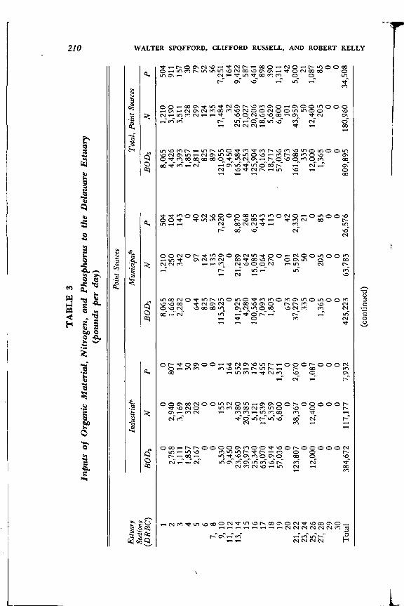
•1

C.., 'TI 'II 0 r' 'TI

'11 0 Cl,

Cl, z 0 ITI

-

TA

BL

E 3

Inpu

ts o

f O

rgan

ic M

ater

ial,

Nitr

ogen

, and

Pho

spho

rus

to th

e D

elaw

are

Est

uary

(pou

nds

per

day)

Est

uary

Sect

ions

(DR

BC

)

Poin

t Sou

rces

Indu

stri

al"

.

Mun

icip

aib

-

Tot

al,

Poin

t Sou

rces

BO

D5

NP

BO

AN

PB

OD

5N

P

10

00

8,06

51,

210

504

8,06

51,

210

504

22,

758

2,94

080

71,

668

250

104

4,42

63,

190

911

31,

111

3,16

914

2,28

234

214

33,

393

3,51

115

74

1,85

732

830

00

01,

857

328

305

2,16

720

239

644

9740

2,81

129

979

60

00

825

124

5282

512

452

7,8

00

089

713

556

897

135

569,

10

5,53

015

531

115,

525

17,3

297,

220

121,

055

17,4

847,

251

11, 1

29,

450

3216

40

00

9,45

032

164

13, 1

423

,659

4,38

055

214

1,92

521

,289

8,87

016

5,58

425

,669

9,42

215

39,9

7320

,385

319

4,28

064

226

844

,253

21,0

2758

716

25,3

405,

121

176

100,

564

15,0

856,

285

125,

904

20,2

066,

461

1763

,070

17,5

3945

57,

093

1,06

444

370

,163

18,6

0389

818

16,9

145,

359

277

1,80

327

011

318

,717

5,62

939

019

57,0

366,

800

1,31

10

00

57,0

366,

800

1,31

120

00

067

310

142

673

101

4221

, 22

123,

807

38,3

672,

670

37,2

795,

592

2,33

016

1,08

643

,959

5,00

023

, 24

00

033

550

2133

550

21

25, 2

612

,000

12,4

001,

087

00

012

,000

12,4

001,

087

27, 2

80

00

1,36

520

585

1,36

520

585

290

00

00

00

00

300

00

00

00

00

Tot

al38

4,67

211

7,17

77,

932

425,

223

63,7

8326

,576

809,

895

180,

960

34,5

08

(con

tinue

d)

z tTJ

C', r C') z z NI z 0 NI

(con

tinue

d)

'a

TA

BL

E 3

(C

oncl

uded

)

C"

Est

uary

Sect

ions

(DR

BC

)

Are

a So

urce

s

BO

A

Tot

als,

All

Sour

ces

NP

Tri

buta

ries

'.

Stor

m W

ater

"

BO

AN

PB

OD

5N

F

11,720'

407

514

1,360

367

103

11,100

1,980

1,120

22,090

931

483

00

06,520

4,120

1,390

30

00

00

03,390

3,510

157

4182

206

238

00

02,040

534

268

52,000

950

425

00

04,810

1,250

504

6

7,

8

9, 10

4,110

211

1,880

1,810

159

564

724

150

439

0

1,810

12,960

0

489

3,499

0137

982

4,940

2,920

136,000

1,930

782

21,500

776

343

8,670

11, 12

13, 14

15

16 17

18

1,500

2,790

17,181

1,430

2,470

879

625

1,785

4,455

563

1,737

1,012

179

431

5,746

299

1,000

1,037

21,260

9,490

18,860 0

1,950 0

5,740

2,562

5,092 0

526 0

1,612

719

1,430 0

148 0

32,200

178,000

80,300

127,000

74,600

19,600

6,400

30,000

30,600

20,800

20,900

6,640

1,950

10,600

7,760

6,760

2,050

1,430

19

00

00

00

57,000

6,800

1,310

20

00

00

00

673

101

42

21, 22

11,900

3,940

1,319

8,320

2,246

631

181,000

50,100

6,950

23, 24

00

00

00

335

50

21

25, 26

00

00

00

12,000

12,400

1,090

27, 28 29

0 0

0 0

0 0

0 0

0 00 0

1,370 0

205 0

85 0

30

00

00

00

00

0

Tot

al50

,343

19,1

4412

,984

76,0

1020

,523

5,76

293

6,24

822

0,62

753

,254


(Footnotes for Table 3)

Note: Organic material is reported in pounds of five-day biochemical oxygen demand(BOD5) per day; nitrogen, in pounds of nitrogen (N) per day; and phosphorus, in poundsof phosphorus (P) per day.

a Industrial loads were estimated from unpublished data supplied by the DelawareRiver Basin Commission.

b Based on 1968 sewage treatment plant discharges, in Delaware River Basin Commis-sion, "Final Progress Report: Delaware Estuary and Bay Water Quality Sampling andMathematical Modeling Project," May 1970. Nitrogen and phosphorus loads were esti-mated from the BOD loads according to data presented in G. A. Rohlich and P. D.Uttormark, "Wastewater Treatment and Eutrophication," Nutrients and EutrophicationSpecial Symposium Volume I (Ann Arbor: American Society of Limnology and Ocean-ography, Inc., 1972).

This quantity does not include inputs from the Delaware River above Trenton.d BOD loads are based on 1964 stormwater overflow in R. V. Thomann, Water Quality

Management. Nitrogen and phosphorus loads have been estimated from BOD loads accord-ing to data given in Environmental Protection Agency, Storm Water Management Model(Washington, D.C.: U.S. Government Printing Office, 1971), p. 180.

Tributary loads are based on the low flow season averaged over a three year period.

resulting plumes of both the aggregated point source and its correspond-ing individual point sources (within the same grid) are the same.44

The area sources from the source inventory were aggregated (or disag-gregated) to the 5 kilometer grid size shown in figures 3 and 4. However,we have made one modification to these sources. From the fifty areasources within our urban-suburban area, we have subtracted the gaseousemissions resulting from household space heating. Particulate and sulfurdioxide emissions from this activity are included in the residuals genera-tion and discharge submodel, and are thus eliminated from backgroundresiduals.

We felt it was necessary to separate aggregated point sources from thearea sources in the region because of the difference in effective stackheights (sum of the physical stack height plus plume rise) of these twotypes of sources.

The estuary and its quality f

For the period October 1912 to September 1965, the mean annual flowof the Delaware River at Trenton, New Jersey, was 11,550 cubic feet per

c

44. This teatment does not, however, insure the same distribution of ground levelconcentrations. The latter is a complex nonlinear function of many arguments includ-ing effective stack height. Emissions close to the ground contribute, proportionally, moreto local ambient concentration levels than do the emissions discharged higher up. Thehigher emissions tend to spread out over the region more. This technique was usedhere as an expedient measure. Consideration of each point source as a separate entityin the air dispersion model would have been an expensive proposition, and the addi-tional accuracy would not have been warranted for the kinds of investigations we aremaking with our Base Model. t


second (cfs). The Delaware is similar to most rivers in the northeasternUnited States with respect to its seasonal variation of flow: maximum

d mean monthly flows are experienced in March and April (20,000 to 25,-Is 000 cfs), and minimum mean monthly flows in the late summer months

of August and September (about 2,500 cfs).45Although a Streeter-Pheips type dissolved oxygen computer model for

the Delaware Estuary is available from the DRBC, we are using theaquatic ecosystem model described in an earlier section. The DO model

P. of this estuary used 30 reaches between Trenton, New Jersey and ListonPoint, Delaware. By combining some of the shorter reaches, we have re-duced this number to 22 in order to save computer time. The DelawareValley Base Model employs 11 of the new reaches: those which lie withinthe area outlined in figures 3 and 4.

The atmosphere and its qualityI. In order to relate ambient concentrations throughout the region with

gaseous residuals discharges, we needed both an air dispersion model anddata on the meteorology of the Delaware Valley region. The atmosphericdispersion model which we are using in the Base Model was presented

a in an earlier section. Necessary data inputs to the model are a jointprobability distribution for wind speed, wind direction, and atmospheric

r stability based on meteorological data for the Delaware Valley region. Weassumed, based on EPA data, that the mean monthly maximum atmos-

I pheric mixing depth for the season of interest is 1,000 meters, and thatthe mean seasonal temperature and pressure for this region are 68°F

e (20°C) and 1,017 millibars (30.03 inches of mercury) respectively.For purposes of the air dispersion model, each of the ten activities

presented in table 1 is treated as a single point source even though mosthave, in fact, several stacks—one, for example, has over 40 stacks listedin the gaseous emission inventory. Where more than one stack was listedfor a particular plant, a "virtual" stack was calculated on the basis of thecenter of mass of the individual plumes. This method of aggregation was

r discussed previously in this section. Stack characteristics which are re-quired by the IPP model for computing effective stack height includephysical stack height, stack diameter, and stack exit velocity and tem-perature of the gas.

ee

45. United States Geological Survey, Compilation of Records of Surface lValers of theUnited States, October 1961 to September 1965: Part 1—B North Atlantic Slope Basins,

e New York to York River U.S. Geological Survey Water.Supply Paper 1902 (Washing-ton, D.C.: U.S. Government Printing Office, 1970).


The computer program

The optimization algorithm we are using consists of a standard linearprogram (IBM's MPSX—360) and four FORTRAN coded subprograms46The algorithm is set up in such a way that two, or more, linear program.ming problems can be solved sequentially prior to entering the fourFORTRAN coded routines (to be described below). Our experience todate indicates that this is a workable arrangement as far as the MPSXsoftware is concerned.

The ten sources in the region for which residuals management optionshave been provided are divided equally between two linear programs,MPSX—l and MPSX—2. Home heating and municipal solid residuals man-agement options for the 50 grid squares comprising the urban-suburbanarea have also been divided evenly between the two linear programs.

Given prices (marginal penalties) on discharges, evaluated in the envi-ronmental and constraint evaluation submodels to be discussed below,these two linear programs are solved, subject to the appropriate con-straints, and the resulting residuals discharges are passed as inputs to theenvironmental models. See figure 5 for overall program flow.

The first of the FORTRAN subprograms, DATA SORT, is used tocall the remaining three, in turn, to aggregate liquid residuals dischargesentering the same reach or section of the estuary, and to assign marginalpenalties to all the liquid residuals dischargers prior to returning toMPSX control for another iteration of the linear programming models.

The next FORTRAN routine, AQUATIC ECOSYSTEM, is the non-linear aquatic ecosystem model. This model computes the steady statevalues for the eleven endogenous variables in each of the eleven sectionsof the estuary; this will be expanded to 22 reaches with the full-scaleDelaware Valley Model. In addition, given penalty functions for exceed-ing standards on various quality measures of the natural world, this rou-tine evaluates total penalties associated with water quality, as well as themai-ginal (water quality) penalties attributable to all liquid residuals clis-chargers in the region.

The third FORTRAN routine, ATMOSPHERIC DISPERSION, isthe linear atmospheric dispersion model. In this routine, steady statelevels of suspended particulates and sulfur dioxide at all ninety-nine grid

46. IBMs linear programming code was used because of its capability for handlinglarge problems, our previous experience with it, and the availability of the IBM 360system for our use.

r0

0

Is

5,

0

I'0

5.

e

Is

e

1—

S.

is

Cl


Figure 5

Schematic Diagram of Program Flow: Optimization Algorithm

Marginal penalties

Residuals discharges

___________________

AQUATIC ECOSYSTEM

Translates residuals dischargesto ambient concentrations,computes marginal penaltiesassociated with water quality

y

MPSX-l MPSX-2

jREAOCOMM(1)

Activity (2) Upper and lower bounds.marginal penalties

DATA SORT

Converts MPS activity levels todistributed residuals discharges,converts distributed marginalpenalties to prices on residualsdischarges.

Residuals discharges.prices, penalties

Residuals Marginaldischarges penalties

<Upper and lower bounds.program controlparameters

IATMOSPHERIC DISPERSION

Translates residuals dischargesto ambient concentrations,computes marginal penaltiesassociated with air quality

OPTIMIZE CONTROL

Calculates objective function.tests icr convergence, computesstepsize, sets "artificial"upper and lower bounds

1. READCOMM is an IBM supplied FORTRAN coded subroutine which allowsinteraction between MPSX and other FORTRAN routines. For a description of its usesee IBM Manual SH2O-0960-0, Mathematical Programming System Extended (MPSX) ReadCommunications Format (READCOMM) Program Description Manual (White Plains, NewYork: IBM, 1971).

2. Indicates an input-output link.

points throughout the region are computed. In addition, total penaltiesassociated with exceeding air quality standards are evaluated, and mar-ginal (air quality) penalties are computed for each discharger in the re-gion.

The fourth and last FORTRAN routine, OPTiMIZE CONTROLcontrols the allowable changes in levels of residuals dischas'ges betweensuccessive iterations, ensures that the new solution, in terms of the ob-jective function value, is better than the previous one, and determineswhen the program should terminate. Specifically, it selects the step sizesat each iteration for the 136 residuals discharge variables in the BaseModel, it sets the artificial bounds (constraints) associated with each

30


discharge variable, and it determines when the procedure has found alocal optimum.

This particular scheme of iterating between a series of linear program-ming problems and FORTRAN routines creates the bookkeeping prob.lem of directing the proper set of marginal penalties and artificial upperand lower bounds to the corresponding discharge activities which arelocated throughout different linear programs. By properly ordering thedischarge activities, and the marginal penalties and artificial bounds, thefirst part of the data can be read by MPSX—l and the second part canbe read by MPSX—2. This ordering takes place in the FORTRAN rou-tine designated above as DATA SORT.

To start the iterative procedure we are currently using, we place zeroprices on residuals discharge activities, and assume an initial set of valuesfor the penalty function parameter, r. Subject to these prices and param-eter values, the linear program selects "optimal" residuals discharge 1ev-els. Marginal penalties, corresponding to these discharges, are then usedas prices on residuals discharges at the second iteration. This gives us afeasible starting point for the steepest ascent type scheme we employ. Atthe "optimum," some of the environmental standards will generallybe exceeded because we are using the exterior point penalty schemeoutlined above. Another set of values for the penalty function pa-rameter, r, in equation 27 is selected such that < for all r, and theoptimization process is continued, and so on until no environmentalstandard, is exceeded by more than a previously specified amount.Because the response surface may be multipeaked, this procedure yields,at best, a local optimum.

One of the step size selectors which we are currently experimenting withis described in our earlier work.47 Another, which is based on the former,will be presented in the next section where we present some results of themodel. Both step size selectors require a set of ranges for the discliargevariables. The feasible range for all 136 discharge variables has beenestimated from a knowledge of the processes and activities employed.

For any given set of penalty function parameter, r, the program iscoded to end computations when any one of the following conditions ismet:

(i) the value of the objective function increases by no than aspecified amount;

(ii) the number of iterations equals the specified maximum number;

47. C. S. Russell and W. 0. Spofford, Jr., "A Quantitative Framework," equation 2.1—18, p. 135.


(iii) the number of different step size sets equals the specifIed maximumnumber.

Some results

Our interest in the computational results lies primarily in the evidencethey afford on the following questions:

Does the heuristic algorithm we have described appear to converge toan optimum when faced with a moderately large problem?

Is the solution obtained characterized by only small violations of theambient environmental quality standards?

Is there evidence that the solution represents a global optimum?What can we say about the effect of various choices for penalty-function

parameters and step-size selector schemes in relation to the above ques-tions?

Finally, is the cost of the computational exercise so high as to promisethat a full-scale regional model would be simply a white elephant?

In this section, we discuss the light shed on these important questionsby five separate runs of the Base Model. These runs are distinguished bythe ways in which the penalty function parameters are handled, and bythe step-size selector employed.

Penalty Function Parameters. Recalling that the penalty functionfor a particular constraint may be written 1/r.p(X), we distinguish thefollowing sets of values for l/r in table 4:

TABLE 4Sets of Values for hr

Indicator

Penalty Function Parameter Set

a b c d

Sulfur dioxide 100 1000 100 10

Suspended particulates 10 100 10 1

Algae 106 106

Fish 106 106

Dissolved oxygen 106 106

Step.Size Selector Scheme. Three step-size selector schemes were usedfor the five runs of the Base Model presented in this section. For all three

5

5


step-size selectors, the initial step-size vector is the same. However, sub-sequent step-size vectors differ.

Given the vector of ranges, R, for all 136 discharge variables, the initialstep-size vector, is computed as follows.

6' = I = 1, . . , 136. (39)

For the first step-size selector scheme, subsequent step-size vectors arecomputed using the following formulation.

(40)

where n is the number of step-size sets.For the second step-size selector scheme, step-size vectors, after the first,

are computed as follows.

= k 1, - . . , n. (41)

The third step-size selector scheme is a little more involved. Ratherthan shortening all elements of the step-size vector proportionately at agiven step-size change (as in the case with the first two schemes), this Se-lector reduces elements of the vector selectively. According to this scheme,at any given step-size change, an element of the step-size vector is eitherreduced according to equation 40, or left unchanged.

We decide whether to reduce the step-size of a particular dischargevariable as follows. First, we try to assess whether the objective functiondecrease, which originally signaled the step-size change, is a result (onaggregate) of discharging too much or too little to the environment. Wedo this by comparing consecutive net benefits (the sum of the net bene-fits of MPSX—1 and MPSX—2 net of effluent charges), and consecutivetotal penalties, for the last two iterations of the management model.

If the total penalties decrease and at the same time the net benefits de-crease, we assume that the step-size change was caused by discharging (onaggregate) too little to the environment. On the other hand, if the totalpenalties increase, regardless of what the net benefits do, we assume thestep-size change was caused by discharging (on aggregate) too much to theenvironment.

Once we have established this, we must then compare, element by ele-ment, the last two sets of discharges, and the last two sets of marginal

nPROBLEMS IN RESIDUALS MANAGEMENT MODELS 219

penalties. Disposition of each element of the step-size vector is summa-rized as follows.

Assume discharge too much. If the discharge increases, and the marginalpenalty increases, change step-size according to equation 41. For othercombinations, leave step-size unchanged.

Assume discharge too little. If the discharge decreases, and the marginalpenalty decreases, change step-size according to equation 41. For othercombinations, leave step-size unchanged.

The Five Computer Runs. The five runs may be described as follows:Run 1: the first step-size selector with 1/r set at level "a" initially and

kept there for 40 iterations;48Run 2: the first step-size selector with 1/r set at level "d" initially, kept

there for 20 iterations, reset to level "a" and maintained for a further 20iterations;

Run 3: the first step-size selector with 1/r set initially at level "d,"changed to level "c" at the first step-size change and to level "b" with thesecond step-size change; the program is allowed to run out to the 40thiteration;

Run 4: the second step-size selector with 1/r set at level "a" initiallyand kept there for 40 iterations;

Run 5: the third step-size selector with 1/r set at level "a" initially andkept there for 40 itel-ations.

Ambient Standards. For each run, the ambient environmental qualitystandards were set as follows in table 5. The standards on the airborneresiduals are much less stringent than current federal standards. Theywere chosen this way only because the Base Model has so few controllablesources relative to the discharges we have included as "background."Standards approaching the cut-rent federal limits are infeasible in this test

48. That these runs all involve stopping after 40 iterations is simply a feature of ourinitially cautious experimentation. Ordinarily the algorithm itself would determine thestopping point.

49. It should also he pointed out that the air dispcrsiori model was not calibratedprior to using it. Because of this, the computed ambient concentrations were somewhathigher than those actually observed in the Philadelphia region. If we use the calibrationrelationships for this model from an EPA air quality study of this region (1967—1968data) and modify the air quality penalty function parameter sets accordingly, com-parable results for our regional residuals management model could be obtained by re-ducing the sulfur dioxide standard in our model to (0.416 x 420 = 174.7) andthe suspended particulaics standard to (35 + 0.532 X 100 = 88.2). For thesecalibration relationships. see EPA, "Application of Implementation Planning ProgramModeling Analysis: Metropolitan Philadelphia Interstate AQRC." Air Quality Manage-ment Branch, Applied Technology Division, Office of Air Programs, EPA, Durham, N.C.,February 1972, (mimeo), figures 2 and 3.

Indicator Location Standard

Sulfur dioxide

Suspended particulates

Algaea

Fisha

Dissolved oxygen

center of each grid square

center of each grid square

each reach

each reach

each reach

�420 b

� 100 b

�2.0 mg/L

�0.29 mg/L�3.0 mg/L

a Based on biomass concentrations in terms of the total weight of carbon, nitrogen,and phosphorus.

b Standards used with uncalibrated air dispersal model.

situation even under the uninteresting policy choice of shutting down allsix industrial emitters and the two municipal incinerators.

Results of the Five Runs. The results of the five computer runs arepresented in tables 6, 7, and 8, and in figures 6 through 10. In table 6,we show, for the five computer runs, production levels at the 40th itera-tion for all six industrial plants and for the two municipal incinerators.In addition, we show production levels for the first iteration (zero priceson residuals discharges) and the second iteration (maximum prices onresiduals discharges). The results of the first two iterations are the samefor all five runs. Also depicted in table 6 are the net benefits (sum of theindividual MPSX objective function values corrected or plus for the efflu-ent charges "paid"), the total penalties, and the objection function valuesat the 40th iteration for the five computer runs.

In table 7, we present for the five computer runs the discharge levelsof air-borne, liquid, and solid residuals at the 40th iteration for the tenactivities in the region for which residuals management options have beenprovided. Also shown are the residuals discharge levels for the first andsecond iterations (which are the same for all five runs).

Ambient concentrations which exceed the standards on the 40th itera-tion are displayed in table 8 for all 5 runs. There we show the standardwhich is violated, the amount of the violation, the location of the viola-tion (estuary reach or air quality grid square), and the per cent violationbased on the level of the standard.

Figures 6 through 10 depict a plot of the objective function value vs.iteration for the 5 runs. Also shown in these figures are the iterations


TABLE 5Ambient Environmental Quality Standards

'a 0 r C', z tTl

CI, r z C, z 0 M

-1

6

Prod

uctio

n L

evel

s an

d O

bjec

tive

Func

tion

Val

ues

for

the

Five

Com

pute

r R

uns

Sour

cePr

oduc

tion

Out

puts

Num

ber

and/

or in

puts

Uni

ts

Iter

atio

nR

esul

ts a

t40

th I

tera

tion

for

Run

s

12

12

34

5

Ref

ined

sug

arto

ns/d

ay40

00

580

050

0

2R

efin

ed s

ugar

tons

/day

400

010

70

4185

5

3E

lect

rici

tyM

W h

rs./d

ay6,

040

06,

040

6,04

06,

040

6,04

06,

040

4E

lect

rici

tyM

W h

rs./d

ay11

,550

11,5

5011

,550

11,5

5011

,550

11,5

5011

,550

5C

rude

oil

proc

esse

dG

asol

ine

bbls

./day

bbls

./day

162,

000

116,

200

0 012

9,30

057

,200

147,

200

70,2

0014

5,30

069

,200

129,

900

57,6

0014

4,30

067

,400

6C

rude

oil

proc

esse

dG

asol

ine

bbls

./day

bbls

./day

172,

000

123,

400

130,

800

53,2

0017

2,00

099

,500

172,

000

123,

400

172,

000

123,

400

172,

000

105,

800

172,

000

121,

000

9So

lid r

esid

uals

pro

cess

edto

ns/d

ay49

50

506

512

516

507

505

10So

lid r

esid

uals

pro

cess

edto

ns/d

ay29

80

298

298

298

298

298

Net

ben

efits

(M

PSX

—1

+$

per

day

492,

300

69,7

0029

7,60

033

5,70

031

7,30

030

6,10

032

9,70

0

Tot

al p

enal

ties

$ pe

r da

y2,

277,

500

01,

600

22,6

0048

,400

800

600

Obj

ectiv

e fu

nctio

n va

lue

$ pe

r da

y(1

,785

,200

)69

,700

296,

000

313,

100

268,

900

305,

300

329,

100

Eff

luen

t cha

rges

not

incl

uded

.

S

I

TA

BL

E 7

ts;i

Res

idua

lsD

isch

arge

Lev

els

for

the

Five

Com

pute

r R

uns

Sour

ceN

umbe

rR

esid

ual

Uni

ts

Iter

atio

nR

esul

ts a

t40

th I

tera

tion

for

Run

s

12

12

34

5

Sulf

ur d

ioxi

dePa

rtic

ulat

esB

OD

Nitr

ogen

Hea

tT

otal

sol

ids

tons

/day

tons

/day

lbs/

day

lbs/

day

106

BT

U/d

ayto

ns/d

ay

6.9

22.1

33,4

002,

790

2,38

0 6.4

0 0 0 0 0 0

0.8

1

134 780

25.4

0 0 0 0 0 0

0 0 0 0 0 0

0.9

1

117 68 0 22

.4

0 0 0 0 0 00

2Su

lfur

dio

xide

Part

icul

ates

BO

DN

itrog

enH

eat

Tot

al s

olid

s

tons

/day

tons

/day

lbs/

day

lbs.

/day

106

BT

IJ/d

ayto

ns/d

ay

6.9

2233

,400

2,79

02,

380 6.

4

0 0 0 0 0 0

1.2

2.3

327

180 0 47

.2

0 0 0 0 0 0

0.7

0.7

95 56 0 18.2

1 2.2

198

116 0 37.1

0.1

0.1

12 7 0 2.3

r

3Su

lfur

dio

xide

Part

icul

ates

Hea

tSo

lids

Slur

ry

tons

/day

tons

/day

BT

U/d

ayto

ns/d

ayto

ns/d

ay

54.4

111.

732

,400 50

.70

0 0 0 0 0

12.4

23.2

5,40

0 66.3

173.

4

17.6

22.5

21,4

00 64.4

152.

2

16.2

21.3

19,5

00 64.9

157.

8

14.3

231,

700 65

.616

5.8

14.3

231,

900 65

.616

5.8

4Su

lfur

dio

xide

Part

icul

ates

Hea

tSo

lids

Slur

ry

tons

/day

tons

/day

106

BT

U/d

ayto

ns/d

ayto

ns/d

ay

104

309.

861

,900 97 0

7.6

9.7

0 70.2

285.

2

58.6

140.

515

,700 11

3.8

187.

6

104

275.

942

,100 12

7.4

0

81.7

226.

737

,100 10

8.2

92.2

66.1

168.

414

,900 11

1.2

156.

6

63.5

184.

611

,000 112

167.

2

0

4

& y

33.4

34.2

3.5

2.4

6,30

04,

500

365

291

943

632

28,0

0050

0

Part

icul

ates

BO

DN

itrog

enPh

enol

sH

eat

tons

/day

tons

/day

lbs.

/day

lbs.

/day

lbs.

/day

106

BT

U/d

ay

148.

213

.612

,500 56

82,

023

53,2

00

0 0 0 0 0 0

33.9 2.4

4,50

029

062

674

0

35.9 3.5

6,50

036

996

3

6Su

lfur

dio

xide

Part

icul

ates

BO

DN

itrog

enPh

enol

sH

eat

tons

/day

tons

/day

lbs.

/day

lbs.

/day

lbs.

/day

106

BT

U/d

ay

157 14

.413

,300 601

2,15

056

,500

10.5 1.3

4,70

032

767

0 0

88.2 7.7

9,80

045

11,

540

27,2

00

28,4

00 157 14

.413

,300 601

2,15

0

7

.

Part

icul

ates

BO

DN

itrog

enSo

lids

tons

/day

Jbs.

/day

lbs.

/day

tons

/day

49.4

272,

500

32,4

00 82.4

2.1

19,5

0011

,400

108.

8

25.4

33,9

0014

,200 93

.4

52,7

00 21.3

27,2

0013

,400 134.

4

8Pa

rtic

ulat

esB

OD

Nitr

ogen

Solid

s

tons

/day

Jbs.

/day

Jbs.

/day

tons

/day

19.1

105,

000

12,5

00 31.8

1.1

7,50

04,

400 55

.9

10.8

27,5

008,

300 58

.4

21.8

72,2

0010

,800

9Pa

rtic

ulat

esSo

lids

tons

/cla

yto

ns/d

ay9.

912

3.9

0 04.

913

1.9

7.4

10Pa

rtic

ulat

esSo

lids

tons

/day

tons

/day

5.9

74.5

0 02.

977

.5

130.

8

4.8

34.4 3.2

6,20

036

191

6 0

96 12.4

12,6

00 571

2,03

052

,900 27

.332

,300

13,9

00 107.

6

19.1

105,

000

12,5

00 31.8

157 14

.413

,300

601

2,15

044

,900 23

.231

,200

15,6

00 148.

9

19.2

58,2

0010

,200 42

.1

101 9.

310

,600

460

1,68

031

,700 28

.634

,000

14,2

00 97.7

12.4

31,8

008,

900 54

.9

(I, C r C,, z C.,

P1

P1 z H 0 P1 t'J

4.5

3.4

5.7

TA

BL

E 8

Vio

latio

n of

Am

bien

t Sta

ndar

ds o

n th

e 40

th I

tera

tion

for

the

Five

Com

pute

r R

uns

Run

Num

ber

ofV

iola

tions

Indi

cato

rU

nits

Loc

atio

n(G

rid/

Rea

ch)

Vio

latio

n,A

ctua

lV

iola

tion,

Per

Cen

t of

Stan

dard

14

Sulf

ur d

ioxi

deFi

shD

isso

lved

oxy

gen

Dis

solv

ed o

xyge

n

mg/

Lm

g/L

mg/

L

59 15 17 15

1.4

0.01

0.03

40.

009

033

3.45

1.13

0.3

25

Sulf

ur d

ioxi

deSu

lfur

dio

xide

Fish

Dis

solv

ed o

xyge

nD

isso

lved

oxy

gen

jsg/

rn3

mg/

Lm

g/L

mg/

L

59 20 15 15 17

5.1

0.5

0.01

20.

130.

053

1.21

0.12

4.14

4.33

1.77

35

Sulf

ur d

ioxi

deSu

lfur

dio

xide

Susp

ende

d pa

rtic

ulat

esD

isso

lved

oxy

gen

Dis

solv

ed o

xyge

n

jig/r

n3Ji

g/rn

3jig

/rn3

mg/

Lm

g/L

59 20 59 17 15

0.5

0.1

0.1

0.17

60.

131

0.12

0.02

0.1

5.87

4.37

44

Sulf

ur d

ioxi

deSu

spen

ded

part

icul

ates

Fish

Dis

solv

ed o

xyge

n

jig/r

n3

mg/

Lm

g/L

59 58 15 17

1.9

0.2

0.00

10.

022

0.45

0.2

0.34

0.73

56

Sulf

ur d

ioxi

deSu

spen

ded

part

icul

ates

Susp

ende

d pa

rtic

ulat

esFi

shD

isso

lved

oxy

gen

Dis

solv

ed o

xyge

n

jig/r

n3Ji

g/rn

3Ji

g/rn

3rn

g/L

rng/

Lm

g/L

59 59 58 15 15 17

1.3

0.9

0.3

0.00

10.

014

0.01

4

0.31

0.9

0.3

0.34

0.47

0.47

iii0 M NI I-

5, PROBLEMS IN RESIDUALS MANAGEMENT MODELS

Figure 6

40

225

where step-size changes occurred (indicated by an "S"), as well as thosewhere penalty function parameter sets were changed (indicated by a

Discussion of the Results. The iterative optimization scheme whichwe are using for the Delaware Valley Base Model can find, or at leastcome very close to finding, a local optimum. It may take a long time, butit will eventually get there. The question we are exploring here is oneof computational efficiency—which step-size scheme in combination withwhich sets of penalty function parameters permits climbing to the opti-mum the fastest. We attempt to answer this question with 5 runs of theBase Model. Caution should be exercised in comparing the results of the5 computer runs, however, because each of the runs meets a different mixof levels of environmental quality (see table 8).

The most significant conclusions to be derived from the results of theruns follow.

n

Objective Function Value vs. Iteration, Run 1

0 10 20 30Iteration


Figure 7


Objective function value,thousand dollars per day40C

S P

350 - / sss300-

250- 1 -200 - -

150 - -

100- -

50- -

C

-50 -

-100 -

-150 —

—200 tittlitillliiilti it LiltllttlLtlltll lit0 10 20 30 40

IterationS indicates a step-Size change.P indicates change in penalty function parameter.

1. Technically, none of the runs have reached an optimum by the 40thiteration, although evidence suggests that Runs 2, 4, and 5 all may hequite close. Plots of typical residuals discharges throughout the iterativeoptimization procedure (not shown here) indicate that Runs 1 antI 3 arequite far from the optimum. We might also point out that of the S runs,Runs I and 3 obtained, by the 40th iteration, the lowest objective Itinc-tion values (see table 6).

2. From the 5 runs presented, it is not possible to ascertain whetherthey are approaching the same optimum or different optima. The ques-tion of local vs. global optimum cannot be answered, but we suspect thatwe are dealing with a multi-peaked response surface.

3. Of the 5 runs presented, Run 5 not only appears to be the mostefficient in terms of its hill-climbing ability (see figure 10), but also itappears to have achieved the best solution by the 40th iteration. Thisconclusion is based on the fact that: on aggregate, Run 5 did one of thebest jobs of meeting the environmental quality standards (see table 8);its objective function value is the highest of the five; its penalties are thelowest of the 5; and finally, its net benefits are the second highest of the5 runs (see table 6).

In addition, there is evidence, albeit weak, to suggest that neither Runs2 nor 4 are as close to the optimum as Run 5. This is shown in the liquiddischarge data (BOD and nitrogen) for source 8, and the sewage treat-ment plant for Wilmington (see table 7). There are no standards violated


Figure 8


Objecttve function value,thousand dollars per day

20Iteration

C

e

e

r

downstream of source 8, yet only in Run 5 are BOD and nitrogen dis-charges at their maximum levels. Both Runs 2 and 4 have quite a wayto go before reaching this upper limit.

4. The penalty function scheme described in this paper was quitesuccessful in meeting environmental quality standards (see table 8). Acomparison of the sulfur dioxide violations for Run 3 (see table 8) withthose of Runs 1 and 2 indicate the effect of increasing the penalty func-tion parameter. Recall that the penalty function parameter for Run 3,on the 40th iteration, is ten times that of either Runs 1 or 2.

5. The third step-size scheme with no change in penalty functionparameter, Run 5, appears to be superior to the other schemes which weretested. However, the step-size choice continues to remain the weakest partof our optimization technique and there is much room for improve-ment.


Figure 9

Objective Function Value vs. iteration, Run 4

Objective function value,thousand dollars per day

0 10 20 30 40Iteration

'1

Ii

11

6. Examination of residuals discharge data throughout the iterativeoptimization scheme (not shown here) suggests that the response surfacein the vicinity of the optimum is relatively flat, at least inside the feasibleregion, and that substantial tradeoffs among different residuals and dif-ferent dischargers, in many cases, are taking place. Examination of thenet benefit function values on the 40th iteration (see table 6) togetherwith the rather significant variations in discharge data for this iteration(see table 7) indicates the same thing. That is, there are wide ranges ofdischarges among the 5 runs, yet the net benefits vary only a few per cent(maximum of between nine and ten per cent for Runs 2, 4, and 5). Thisdifference is even more pronounced when net benefits and discharge datafor Runs 2 and 5 are compared.


Figure 10


L


Costs of a Computer Run. What can we say about costs, and theprospects for running a much larger version of this model within a rea-sonable computer budget? To place this question into some perspective,we summarize, in the following table, the size, in terms of the numberof rows and columns of the LP submodels, of the Delaware Valley BaseModel.

TABLE 9Size of LP Submodel

—Delaware Valley Ba.se Model—

MPSX-1 MPSX-2 Total

Variables (columns)Total 320 320 640Residuals discharges 68 68 136

Constraints (rows)Total 178 178 356Equality 135 135 270Inequality 43 43 86

Step-size bounds (rows) 136 136 272

S

t4

r

foj

air

res

ofpnare

The aquatic ecosystem model comprises 11 reaches of the estuary, witheach reach requiring a set of 11 nonlinear differential equations. Thisresults in a total of 121 equations for describing the aquatic system withinthe limits of the Base Model. The number of reaches to be considered inthe full-scale Delaware Valley model will be expanded to 22. Thisamounts to an eventual doubling of the size of the aquatic ecosystemmodel.

The air dispersion model includes 11 point sources, 44 "aggregated"point sources, and 99 area sources for a total of 154 sources. Ambientconcentrations are computed for 99 receptor locations. In order to ps-e-dict the ambient concentrations of sulfur dioxide and suspendedlates, one 154 by 99 element matrix of transfer coefficients is required foreach residual. It is difficult to estimate at this time how many sources willeventually be considered in the full-scale Delaware Valley model, but thereceptor locations probably will not be increased by more than 50 pet'cent.

The cost per iteration of the Base Model is about $8.70 for the cur-

50. This is based on a CPU running time of 0,42 minutes per iteration on an IBM360—65 with a core requirement of 300 K.


erent A large fraction of this cost is for internal input-output time (65 per cent); a smaller fraction for central processing unit(CPU) time (26 per cent); and the smallest part for computer printout(9 per cent). It goes without saying that there are large savings possibleif the number of iterations required to reach, or at least come close to,an optimum can be reduced through more efficient means of selectingstep-sizes and sequences of penalty function parameter sets. It is our planto continue to search for more efficient combinations. But the cost infor-mation above also implies that there are potentially large savings fromreducing the quantity of information which must be stored and trans-ferred in and out of core with the various submodels each iteration.

One possibility for saving internal input-output time would be to in-clude the linear air dispersion model within the constraint set of theresiduals generation and discharge LP submodel. This would involveadding 198 rows (99 for ambient concentrations of sulfur dioxide, andanother 99 for suspended particulates) to the Base Model, but could re-duce the internal 1—0 time by, perhaps, ten per cent. In addition, it wouldprobably improve the efficiency of the iterative optimization scheme sincein this case penalty functions would be needed only for standards onalgae, fish, and, dissolved oxygen. However, a major drawback of this

— approach is that individual (unlinked) LP submodels, in general, wouldnot be possible with this scheme and some form of decomposition would

his be necessary to deal with model size.We are currently searching for other ways to reduce internal input.

in output time, even at the expense of increasing CPU time, and plan tohis investigate some of them with the Delaware Valley Base Model.em As for cost increases with model size, the problem appears serious, but

certainly not serious enough to abandon the project at this point. It ap-pears to us that, currently, most of the CPU time is used for sorting both

ent discharges and marginal penalties, for controling the program flow, and)re- for the solution (including penalties and marginal penalties) of the envi-

ronmental submodels. CPU costs, however, should not increase in pro.for portion to the increase in the number of discharges because many of the

will computations necessary to set marginal penalties at each iteration arethe already being done in the Base Model.per On the other hand, the input-output time required for the transfer of

residuals discharges, marginal penalties, and the changing upper andcur- lower bounds on each discharge will increase linearly with the number

of discharges. This is a problem, and one which lends little hope for im-

IBMprovement as long as nonlinear simulation models of the natural worldare included within the optimization framework. But as noted above, this

In232 WALTER SPOFFORD, CLIFFORD RUSSELL, AND ROBERT KELLY

time requirement for the Delaware Valley model could be reduced sub-stantially as long as we remain with linear atmospheric dispersion models

I

and include them as part of the constraint set of the LP submodel.The costs of solving the MPSX packages themselves appear to be a -

relatively small part of the problem, at least at this time, but it also ap.pears that it will be more efficient to have a few large MPSX LP's rather 1

than many smaller ones. The primary reason for this is that each MPSXmodule has certain minimum internal input.output requirements inde.pendent of its size. Ii,

On balance, we are hopeful that the model size can be increased con-siderably with a substantially less than proportional increase in the costof a computer run.

Summary and Conclusionssi

In the Introduction, we presented, very briefly, our regional residualsmanagement framework and indicated that two didactic applications tohypothetical regions had previously been made and are reported else- cwhere. In the first application, both demand functions and economicdamage functions were assumed, and the institutional framework envi- asioned was a regional management authority. In the second application,the model was expanded to provide information on the socio-geographic fdistribution of costs and benefits associated with meeting different levelsof environmental quality. The institutional framework envisioned forselecting levels of environmental quality was a legislative body. We fur-ther indicated in the Introduction that the main purpose of this paper s

is to explore the computational problems associated with scaling up from c

small didactic models to a large scale regional application.We have discussed, in some detail, the problem of model size and

ways to cope with it, and also presented a way to include nonlinear omodels of the natural world within an optimization framework. As a n

means for testing our ideas and techniques for dealing with some of n

the computational problems presented we constructed a relatively simple u

residuals management model of the Delaware Valley region. This ap. oplication is referred to by us as the Delaware Valley Base Model. Resultsof five computer runs indicate that our optimization scheme, whichallows for the inclusion of nonlinear models of the natural world, isoperationally feasible, but that more work is necessary to improve thecomputational efficiency of the procedure so that computer costs can be e

reduced.


In conclusion, there is no question that the management model we areexperimenting with is more complex than previous residuals managementmodels, and that it requires a substantial amount of computer resources.Three questioiis we face and hope to answer as a result of our researchefforts on large scale regional residuals management models are as fol-lows.

I. Is it necessary to include all forms of residuals within a single com-putational framework? In principle, it is necessary, but in practice, doesthe additional simultaneous information on air and water quality, antion the generation of solid residuals, warrant the added effort and ex-pense?

2. Nontreatment management options such as changes in productionprocesses, raw material input mixes, and product specifications, and by-product production and recycling, have all been shown (under some cir-cumstances) to be less costly alternatives to reducing, or modifying, re-siduals than waste treatment alternatives, but can we consider even aportion of these alternatives for a large complex region consisting ofmany different types of economic activities without (a) exceeding thecomputational reliability of present day computer hardware and soft-ware; and (b) exceeding the computer budget of a waste managementagency given that the first condition could even be satisfied?

3. Models of aquatic ecosystems are able to provide additional use-ful information for making public policy on environmental resources,but (a) can we incorporate these models within an optimizing frameworkwithout completely expending the computer budget of a regional resid-uals management agency; and (b) is it necessary to go to nonlinear eco-system models given all the other uncertainties, in both data and modelcomponents, in the other parts of the regional residuals managementmodel?

Our research to date indicates that the of nonlinear modelsof the natural world within an optimization framework is expensive, butnot unreasonably so. Whether it is necessary to include these nonlinearmodels, or whether it would suffice to employ linear models of the nat-ural world, we cannot say at this time. We are currently in the processof exploring this question.

Regarding the second question, given that the intent of our regionalresiduals management modeling effort is to be able to generate distribu-tional information on costs, benefits, and environmental quality for awide range of alternative management strategies for meeting ambientenvironmental quality standards, a priori elimination of management op-tions, in many cases, would be a difficult, and at best arbitrary, task. Our

1

t

S

)

C

C

S

r

r

:1

ra

If

e

:s

h

Is

ee


research thus far has shown that nontreatment alternatives are frequentlyless costly than the more traditional abatement alternatives, but evenmore important to us, it has shown that, in most cases, a priori selectionof alternatives for least-cost solutions is not possible because of all thelinks—both market and nonmarket—which exist for any complex situa-tion. in order to be able to provide as many management options in theregional model as seems desirable for the Delaware Valley region, we planto continue to search for ways of coping with model size.

Finally, as far as the first question is concerned, none of us will knowthe answer to this until someone or some group tries an integrated ap-proach to residuals management modeling and compares its output withthat of other kinds of residuals management models.

COMMENT j

J. Hayden Boyd, The Ohio State University ti

1:1

The paper by Spofforci, Russell and Kelly is a progress report on theDelaware Base Model, an ongoing, large scale modeling effort at Re- si

sources for the Future. An earlier paper by Russell and Spofford alsoreported on the progress of the model, and gives much useful backgroundon its conception and planning.' Two sorts of questions naturally arisein examining a paper such as this. First, what are the technical goals ofthe modeling effort which it describes, and how well have these technicalgoals been achieved? Second, what are the nontechnical goals of themodel? That is, how do the authors plan to use the model to increasethe value of our environment, as we consume its waste disposal and en-vironmental quality services?

The authors wish to advance the state of the art in several ways. First,several waterborne, airborne, and solid wastes, and several aspects ofwater anti air quality, are considered simultaneously. For waterbornewastes and water quality, the model contains 11 endogenous variables,including 5 residuals (N, Ph, BOD, phenols, heat), and 3 quality pa- y

rameters (algae, fish, DO). For air, sulfur dioxide and particulates are 5

modeled. Solid wastes such as furnace bottom ash, digested sludge frommunicipal sewage plants, wet scrubber slurries, and municipal solid wastes di

are also included. Second, the environment is modeled using a nonlinear t1

1. Clifford S. Russell and Walter 0. Spofford. Jr., "A Quantitative Fraiiicwork for gResiduals Management Decisions," Environmental Quality Analysis. Allen V. Kiiecseand Blair T. Bower (Baltimore: The Johns Hopkins Press, 1972).


aquatic model and a linear atmospheric model. The linear atmosphericmodel is simple and straightforward, while the aquatic model is quitecomplex and expensive to compute. The authors claim that "nonlinearrepresentations of the natural world increase the complexity and numberof calculations ncessary for each iteration, but also they increase both therealism and predictive capability of the model." They present no evidenceto support this conclusion.

Third, and significantly. the authors are modeling production modifi-cations in ten waste dischargers. They are allowing the amount of wastegenerated to be modified as a pollution control strategy, and they are alsolooking at trade-offs among wastes. For example, sewage treatment pro-duces sludge which when burned produces particulates which can beprecipitated and carried to a landfill.

This is an impressive and ambitious list of technical features, and rep-resents an advance in the state of the art. The talents of competent sys-tems analysts and the capacities of a large digital computer are challengedby an effort of this scale. It is important, however, to keep perspectiveby considering what the authors were not able to do. They did not con-skier alternatives such as regional treatment plants or bypass piping tomove discharge points elsewhere in the estuary. These kinds of alterna-tives typically reduce the cost of achieving a given level of water quality.They did not consider expansion and contraction of the scale of currentwaste generators, not to mention the options of entry and exit from theregion. Stochastic elements or cyclical variations in waste generation or inenvironmental reaction were not considered. Environmental modifica-tions (for example, low flow augmentation) are not studied in the pres-ent paper, although the earlier paper by Russell and Spofforci indicatedthat at one time there were plans to include environmental modifications.Explicit demands for environmental quality (the so-called "damage func-tions"), also included in the earlier plans, have apparently been dropped.

How well have the limited, albeit ambitious technical goals beenachieved? As the authOrs are the first to acknowledge, the results are notyet in. The model is complex enough that analytical solution is irnpos-

e sible, and gradient methods must be used. There is little theory aboutwhich hill climber is fastest or how to speed up convergence. I have no

:5 doubt, however, that the authors will succeed in solving these knottyr technical problems.

In its present form, the model is far short of fulfilling the authors'technical goals. Only ten waste clischargers are modeled explicitly. "Back-ground" residuals seem to dominate environmental quality. Shuttingdown the ten modeled sources would not meet federal standards, but


adding more sources explicitly will only add to computational difficulties.There were also some expositional difficulties. I had difficulty following

the description of the industry submodels. Several alternative techniquesfor shoehorning the industry models into the overall model were de-scribed, but it was not indicated which one was actually being used. Theinference is that the outputs of plants are allowed to vary as a pollutioncontrol strategy, since imports seem to be a substitute for the plants' out. aputs in some cases. But, I was not able to find an explicit statement abouthow plant outputs do, in fact, vary as part of the overall strategy of poi-lution abatement. It is not clear exactly how the choice between lowsulfur fuel and high sulfur fuel for household heating is being handled.Finally, the explanation of why penalty payments on discharges oughtnot to appear in the overall objective function was hard to follow. Thereason is of course that while a payment for this service is a cost to the asFirm, it is not a cost to society, as it represents a rent on the scarce envi- ajronmental resource.

The particular gradient method which the authors have selected de-serves further comment. The "penalty functions" may appear to be sur-rogate prices on effluents, but they are not. The marginal penalties go tozero as the environmental quality constraints are met. In fact, it is this g'very feature which leads to computational difficulties, because the algo- trithm gets progressively "lazier" in the vicinity of the feasible region. aThe l/r parameters are designed to give an extra push as the feasibleregion is approached. The behavior of the algorithm reflects the implicit Ill

economic assumption made by this and other such programming models:that the demand for the constraint is zero elastic. In other words, im- tprovements in environmental quality beyond the standard are valueless, s

while violations of the standard cost infinite consumer surplus, so that t

the standards will be met (if at all possible), whatever the cost. The pen- S

alty or exterior point method of programming temporarily relaxes athe constraint as a computational expedient, but the end result is a maxi- 0

mum which lies in the "feasible" region.Environmental quality constraints are always somewhat arbitrary, par- P1

ticularly here where background residuals are so high that the federalstandards can't be met in any case. It would be better to retain in the (9model an explicit demand function for environmental quality, even if ithas to be assumed at this stage of our knowledge. The aquatic and at-mospheric models could then compute the marginal opportunity cost of a

the pollutant disposal services of the environment and pass them to theindustry submodels as charges. These effluent charges would not Ui


go to zero as the feasible region (satisfying a set of arbitrary environmen-tal quality constraints) is approached. An explicit quality demand func-tion may help to speed up convergence of the model. Even if not, it wouldcertainly make easier the economic interpretation of the model's solu-tions.

The overall goal of the modeling effort is to help rationalize the man-agement of the environment. Neither in this paper, nor in the earlierpaper by Russell and Spofford, is the institutional framework withinwhich this model is to be used discussed in detail. But the authors do envi-sion a regional management authority with power to set effluent chargesor standards. In other words, the authority has ownership rights in theenvironment, and allocates its capacity among various outputs, includingthe absorption of various kinds of wastes and the provision of variousaspects of environmental quality. The model is to be a staff tool for suchan authority.

Regional environmental management models are not new, but as yetthey have been little used to guide the actual allocation of the environ-ment's scarce services. Any attempt by a regional authority to ration theenvironment's waste absorption services affects the wealth of dischargers,giving incentives to combine with others to use the political mechanismto influence the effluent charges or standards. If the regional managementauthority uses effluent charges, raising charges to reduce effluents results

e in consumer surplus losses to the dischargers. If discharge standards areused, pollution reductions cause changes in both consumer surplus andthe implicit expenditure rectangle associated with the consumption ofthe environment's waste disposal service. If a systems analysis techniquesuch as the Delaware Base Model is used to get a 'least cost" solution,

it there may be severe transfers of relative wealth among dischargers, assome are cut back more than others. Next year's model, which considersa different set of alternatives, may lead to quite a different distributionof relative wealth. The political system seems to resist procedures whichlead to capricious wealth transfers. In the absence of institutions for side

r- payments, it deems to serve up uniform treatment standards (e.g., sec-ondary treatment for all, best available technology), even when lower(total) cost solutions have already been documented.

it According to the authors, the purpose of this paper is to answer thequestion, "Have we developed a mildly interesting academic curiosity ora potentially useful management tool?" One infers that the authors be-lieve that if the computer program should converge fairly rapidly thenthe Delaware Base Model is a useful management tool. Yet, in the ab-


sence of innovative institutions to cope with the wealth transfer prob-lem, it seems doubtful that this model will actually lower the social costof a clean environment.

One object of this modeling effort is to "find a 'best' set of policy in-struments (charges and limits) for imposition by . . . the authority." 2The authors wish to shed light on the choice among alternative allocatinginstitutions: standards (allocation by fiat) vs. use of the price mechanism;effluent charges vs. discharge rights (perhaps auctioned, perhaps transfer-able among polluters).

I wonder if a super systems analysis, modeling simultaneously as manyrelevant aspects of the universe as can be put into the computer, is reallythe vehicle to answer such questions. Disaggregated, piecemeal researchwould seem to be indicated, rather than a large scale computer model,to inform the choice among alternative allocating institutions. We needevidence on information requirements and administrative costs. Whatabout the ability of alternative institutions to cope with stochastic andcyclical elements in waste generation and in the environment? Whatabout the effects of the choice of institutions on the growth and decayof various industries? What about the ability of institutions to cope withthe entry and exit problem? hI

The Delaware Base Model surely has social utility even if, because ofthe expense of its computation, it turns out to be a "mildly interestingacademic curiosity." But it would seem that much information beyondthat capable of being generated by such large scale models is required toaid in our search for a better environment at least social cost.

62. Russell and Spofford, "A Quantitative Framework," p. 119.

44

Documents

Operational Problems in Large Scale Residuals Management Models