OPERATIONAL ANALYSIS OF A JOB SHOP

Stephen C. Graves

Alfred P. Sloan School of ManagementMassachusetts Institute of Technology

Cambridge, MA 02139February 1984 WP1552-84

OPERATIONAL ANALYSIS OF A JOB SHOP

ABSTRACT

We propose and develop a discrete-time, continuous-flow model with

linear control for studying the operation of a job shop that sees a

stationary input mix of job types. We are not concerned with issues

of detailed scheduling, but rather hope to develop a planning tool for

a job shop operation. With the model we are able to characterize the

operational behavior of each work center in the job shop for a given

control policy. The control rule that we assume sets the production

rate at a work center as a fixed proportion of its queue level in each

time period. This control rule is consistent with the assignment of a

planned lead time to each work center. For such control rules the model

gives the steady-state distribution of the production levels at each

work center, as well as the distribution of queue lengths. We show how

to use the model not only to evaluate a specification of the control

rules but also to find a good specification of the control rules that

results in acceptable shop behavior.

1

1. Introduction

The intent of this work is to develop a model-based framework for

performing an operational analysis of a complex batch or discrete-part

manufacturing operation as typified by a job shop. The focus of the

operational analysis is on understanding the interrelationship and inter-

play of the three key components in a manufacturing operation, namely

the available production capacity, the inherent variability and'-uncertain-

ty of the production requirements, and the level of work-in-process in-

ventory. We are interested in understanding how job flow time, or

equivalently the level of work-in-process (WIP) inventory, depends upon

production capacity at each work center or production stage. Similarly,

we want to understand how job flow time relates to the variability of

production requirements that comes from the inherent job mix faced by

the manufacturing operation. To do this we present and illustrate a

mathematical model that. permits such analyses in the context of a job-

shop operation.

A job shop is a very flexible production facility that consists of

a set of versatile machine centers or work stations, and is capable of

producing a wide variety of jobs. The processing requirements for each

job consist of an ordered set ot tasks where each task is to be performed

on a distinct machine center. These processing requirements, as specified

by the tasks, dictate how the job is routed through the machine centers

in the job shop. Due to the wide variety of jobs (i.e. routings) processed

by the shop, it may not be possible to discern any strong pattern in the

flow of work through the shop. In particular, a machine center may receive

jobs from several other machine centers; likewise, jobs at the work center

may. go next to one of several other work centers or may leave the shop

if completed. Because of this lack of dominant work flows through the

2

shop, production control is often very difficult in a job shop. Indeed,

it is often not possible to have very sophisticated production control

because of the cn lexity and variety of work flows.

Production control is often based on a queue management system.

This approach views the job shop as a network of queues where each work

center is a server and the jobs waiting there form its queue. For each

work center we assign a planned lead time that represents the expected time,

both waiting and in process, that a job will spend at that work center.

Production control, in its crudest form, just prioritizes the jobs in

queue at each work center, typically by means of some measure of the

perceived urgency or criticality of the jobs. Job criticality is usually

specified as a function of the difference between the need or promised

date for the jcb and the projected completion date of the job based on the

planned lead times (i.e. job slack), Jobs with the least slack get highest

priority. The projected completion date reflects the processing time and

expected queueing time (i.e. the planned lead times) for each remaining

task for the jcb. '7is prioritization or sequencing of jobs in each queue

is myopic since it is virtually ipossible to anticipate fully how all jobs

will complete heir rocessing through the shop.

A somewha: more sophisticated scheme for queue management is input/

output control ('ht, 1970). ere, the intent is to manage the flow of

work through the sho so that the size of the queue at each work center

remains reaiveelv s=able about a predetermined level. Clearly to do this,

one needs to cr.ro thneinput rate to each work center to match the

output rate. ---s :s relatively straightforward for the work centers at

which ne' jcbs enter the shop; namely, new jobs are released to the shop

at a rate in =ccr-acnce with the roduction rate of the "gateway" work centers,-

However, it is rn-t at all clear how to maintain input/output control at

3

non-gateway work centers, especially if they receive input from multiple

sources. Nor is it all clear how to determine the proper queue levels

about which to target the input/output control.

In this paper we present a model that, in a particular way, formalizes

Wight's concept of input/output control. In the model we describe a queue

management system that relies on planned lead times, as is common in pro-

duction practice. However, we are not concerned with detailed scheduling

issues, and do not use the planned lead times to prioritize jobs; rather

we use the planned lead times for planning the operation of the shop, and

in particular to prescribe the production rates by work center by time period.

This is done in order to achieve some level of input/output control at all

work centers. As we will see, the planned lead times are the key decision

parameters for implementing this form of input/output control.

Most of the previous research on job shops has been in the area of

detailed scheduling, with two major thrusts. One thrust has been research

that explores the performance characteristics of various myopic sequencing

rules. This research has relied upon simulation studies that compare the

performance of a prespecified set of sequencing rules on a particular job

shop with a particular job mix; Conway, Maxwell and Miller (1967) give

an excellent illustration of this type of work and review some of the

earliest studies. A second research thrust has been to determine optimiza-

tion methods for finding the best way to sequence a given set of jobs

through the shop. This research views the scheduling of a job shop as

a large combinatorial-optimization proble=, to which highly specialized

solution procedures may be applied. Lageweg, Lenstra and Rinnooy Kan

(1978) give a good illustration of this type of research, as well as provide

a review of earlier work.

4

There has not been much work that has tried to step iback from the

very detailed issues of sequencing to consider the broader issues of

planning in a job shop. A noteworthy exception is the work of Jackson

(1957, 1963) on queueing networks. This work provided a model for character-

izing the flows through a complex job shop. From this model one could get

insights into the relevant planning tradeoffs between additional capacity,

reduced flow times, and an altered job mix. Other work that has focused on

planning issues is that of Jones (1973), Holstein and Berry (1970, 1972),

Bertrand (1981), and Bertrand and Wortmann (1981). Jones gives an

economic framework for considering the costs of idle resources, of carrying

inventory, of missing due dates, and of making extended due date promises;

the decision variables in the framework are the level of work-in-process

inventory, the tightness of the promised due dates and the sequencing rule.

Holstein and Berry explore the development of a work flow matrix to help

identify the dominant flows in a job shop and to serve as a guide for

smoothing the work flow in the shop. They also show how to use the work

flow matrix to make labor assignments and transfers. Bertrand (1981)

and Bertrand and VWortrmann (1981) evelop and apply a model that strives to

control the flow time of jobs by controlling the aggregate work load in

the shop. They model the behavior of the shop at a very aggregate level

and provide a discrete-time analysis of the flow of jobs through the shop.

Ir this respect their model and analysis are similar to that given in this

paper.

There has recently been work that focuses on understanding the impact

of lot sizing on shop behavior. Karmarkar(1983 ) proposes a simple queueing

model to exam.ine the relationships across lot sizes, manufacturing lead

-5-

times and resource utilization. Zipkin (1983) also uses queueing models

to model a production facility; he then develops an optimization

framework that combines queueing considerations with inventory considerations

in order to set lot sizes for a multi-item, batch production system. These

papers are similar to the current paper in their recognition of the

importance of understanding and controlling sho.p floor time. They focus

on the use of lot sizing to control flow time, while the current paper

does not consider lot sizing at all. Rather, the current paper uses

production rates as the mechanism for control.

The current paper presents a new planning model for analyzing the

operation of a job shop. We will try to argue that this model is a valuable

addition to the existing array of planning models. The remainder of the

paper is organized into three sections. The next section develops the model.

ine model represents the job shop as a continuous-flow, discrete-time

system with linear control. Section 3 gives an illustrative example that

shows how the model might be used to analyze the operations of a job shop.

Section 4 gives a discussion of the model and its assumptions, indicates

how the model might be generalized, and indicates how the model compares w::h

alternative approaches.

6

2. Model Development

This section presents the model that underlies the intended operational

analysis. First we present the assumptions of the model and develop the

basic operational equations that describe the shop behavior. Next we

provide the analysis of these equations that allows us to characterize

the work flow. Finally we show how to determine the effect on the work

flow from marginal changes in the shop parameters.

We base the analyses on a discrete-time model of the job-shop operation.

Implicit in the model is an underlying time period that governs the

transitions within the model. The model assumes that the movement of jobs

from one work center to another, as well as the arrival of new jobs to the

shop, can occur only at the start (or equivalently the end) of a time period;

that is, a job completed during a time period at a work center moves to its

next work center at the start of the next time period. Clearly, we must

choose the time period carefully in order for the model to be a meaningful

representation of the ob shop under consideration. On the one hand, the

time period should be short enough so that it would be highly unlikely that

one job would move through two successye work centers during one time

period. Yet, on the other hand, the tine period should be long enough so

that each work center is capable of completing a handful of tasks during

each time period. (The reason for this statement will be clearer after

we present the model.) he time period is clearly dependent upon the shop.

In some shops the job movement may be such that a two-hour period is

appropriate, whereas in other shops a mlti-day period may best correspond

to the way jobs move.

The model is a ccntinuous-flow model in which we track work loads

rather than jobs. As ill be seen, we express the arrivals to the work

center and the cueue at the work center in terms of the backload (e.g.

hours) for the work center rather than as the number of jobs. Si..ilarl

7

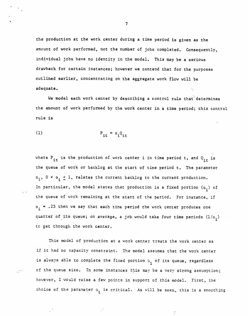
the production at the work center during a time period is given as the

amount of work performed, not the number of jobs completed. Consequently,

individual jobs have no identity in the model. This may be a serious

drawback for certain instances; however we contend that for the purposes

outlined earlier, concentrating on the aggregate work flow will be

adequate.

We model each work center by describing a control rule that determines

the amount of work performed by the work center in a time period; this control

rule is

(1) Pit iQit

where Pit is the production of work center i in time period t, and Qit is

the queue of work or backlog at the start of time period t. The parameter

ai' < ai < 1, relates the current backlog to the current production.

In particular, the model states that production is a fixed portion (i) of

the queue of work remaining at the start of the period. For instance, if

i = .25 then we say that each time period the work center produces one

quarter of its queue; on average, a job would take four time periods (l/ai)

to get through the work center.

This model of production at a work center treats the work center as

if it had no capacity constraint. The model assumes that the work center

is always able to complete the fixed portion ai of its queue, regardless

of the queue size. In some instances this may be a very strong assumption;

however, I would raise a few points in support of this model. First, the

choice of the parameter ai. is critical. As will be seen, this is a smoothing1

8

parameter. We set the parameter ai such that the resulting time series

for production is consistent with available capacity at the work center, i.e.

we need set ai so that we are assured that Pit is achievable most of

the time. Second, the model asserts that the production rate varies directly

with the queue length. This says that when the queue grows, the work

center works harder, and vice-versa.. There is evidence, albeit primarily

anecdotal, that complex shops behave in this manner, especially-when

production is both labor and machine-constrained (e.g. Gomersall 1964)

As a queue builds at a work center, a manager will direct more resources

to the work center to reduce the queue to normal levels. This may entail

shifting workers to the heavily-loaded work center, or working overtime,

or working more efficiently (e.g. postponing maintenance or other non-

productive activities). SImilarly as a queue at a work center drops

below its noLal level, the manager may divert resources away from the

work center. Labor may be shifted to other work centers, and more non-

productive activities such as maintenance, training, and trial.production

will be undertaken.

Although we can view this model of work-center behavior as a descriptive

model, we primarily think of it as being prescriptive of how a shop should

be run. The model lends itself to cases where production control in the

shop is based on planned lead times at each work center. If the planned

lead time at a work center is n time periods (n>i), then the work center,

on average, must process /n of its queue each period. But this is what

(1) does; the control rule prescibes that exactly 1/n of the queue be

processed each time period, where ai = 1/n. Furthermore, we will see that

this control rule not only is consistent with the planned lead time, but

9

also acts to stabilize the work flows through the shop. Each work center

behaves as a filter that smooths its arrival stream of work before passing

the work onto other work centers. Indeed, we will argue that a shop ought

to be managed in this manner.

Now to use (1) we need specify the queue level Qit' The first step

is to pose the standard balance equation

(2) Q = Q -P +A(2)it ii, t-l it

where Air is the amount of work that arrives at work center i at the start

of time period t. By using (1) to replace Qit in (2), we obtain

it ( i) i,t-l + i it'

which is a simple smoothing equation. By repeated substitution, we can

then write production as

S,

S=O(4) P = ' o i (1-H ) s

where we assume we have an infinite history o arrivals. Thus we see

that the production model given by (1) is effectively a simple smoothing

function where the output time series (production) is just a smoothed

version of the input time series (arrivals). If we can characterize

the arrivals to the work center, then we can characterize the production.

For instance, if the elements of the time series {Ait) are i.i.d. random

variables with mean and variance c2 , then we find that

2,_it =and Var{P

it' 2a-

10

Unfortunately, though, the arrival stream to a work center in a job shop

will not consist of i.i.d. random variables. Rather the arrival stream will

tend to be highly correlated over time, as will be seen. Consequently, a

more complex derivation is needed to characterize the time series {Pit}.

The arrival stream to a work center is comprised of two types of flows.

One flow consists of new jobs entering the shop that have their first

processing step (task) at this work center. The second flow consists of

jobs in process that have just completed a processing step at another work

center and have their next processing step at this work center.' We describe

the arrival process to each work center from each other work center by

(5) Aijt = ¢ijPj,t-1 + ijt

where Aij t is the amount of work arriving to work center i from work center j

at the start of time period t, 0.. is a positive scalar, and .. is a

random variable .with zero mean. That is, every time unit (e.g. hour) of

production at ork center j generates C.. times units (hours) of input ec

work center i, o average. The term ijt is an error or noise' term tat

introduces uncerainty into the relationship between production at worr.

center j and i.puts to work center i. iWe assume that for each pair (i,.

the elements in, the time series {.Ejt } are i.i.d.

We offer two comments with regard to (5). First, we have made a

strong assurmption ere that we can model the work flow using a Markov

property. Iha: is, we assume that the arrivals to work center i fro. wcr-

center j do no: depend on how that work got to j. In essence, we assure

that each time period work center j processes a relatively stable or

representative mix of jobs, so that subsequent inputs to downstream wcrk

centers are si.llarlv stable. Tne validity of this assumption depends

upon overall s:ailitv of the job mix in the shop, as ell as the length

of the time e-riod. If the job mix varies drastically (in terms of

11

production requirements by work center) from one week to another, then the

assumption may not be very good. Similarly, if the period length is

such that at most only a few jobs are completed at-the work center each

time period, then it may be unlikely that there is a very stable output.

The second comment concerns how uncertainty or noise enters the

relationship between production at j and inputs to i. One might argue that

the noise should be proportional to the volume of production at work center

j; namely, we might expect with greater production volume, we would have

greater variability in the input stream to i. In (5) the noise term is

independent of the production level. As will be seen, this assumption

permits a great deal of tractability in analyzing the model. Clearly the:

validity of this assumption would have to be examined in the light of

actual shop data.

Now the arrival stream to work center i is given by

(6) Ai = Aij. + itit . iJt

w:Here Nit is a random variable that represent the work load fror new jobs

tnat enter the shop at time t and have their first processing step at work

center i. We assume that for each work center i the elements of the time

series Nit} are i.i.d. We now substitute (5) into (6) to get

(7) Ait = 'C + i

where

t -. . ..it it -ij3t

12

Thus it represents the part of the arrivals that are not predictable from

the production levels of the previous periods, i.e. the new arrivals and the

noise in the flows from other work centers. By assumption, the elements

of the time series { it} for each work center are i.i.d. Note that the

expected values of it equals the expected amount of new arrivals each time

period to work center i.

We are now ready to perform the analysis of the job shop model

specified by equations (3) and (7). It will be convenient to rewrite these

equations in vector notation as

(3') =D)P D A

(7') A P + Et-t -t-1 -t

where P ½ .,P ' A = { ,..., ' are-t= 'lt' nt' t t' 'Ant' t lt' nt

column vectors of random variables, n is the number of work centers, I is

the identity matrix, D is a diagonal matrix with a{l'' .'n } on the diagonal,

and C is an n-bo-n matrix with elements . By substituting (7') into

(3') we obtain

() P = ( - D + Dt)P_ +DE(8) -t (- - == t-l = -t

By repeated substitution we can rewrite (8) as a geometric series

(9) = 7 (I D+ D) s D t-s(9) = I - %t-s

s=0

where we assume an infinite history of the system exists. We use

(9) to characterize the joint distribution of the production vector Pt

lo do this, we let the noise vector t have mean , = ftl,...,.n and a

covariance matrix given by L = {j. We note from the definition of it

that its mean, i' corresponds to the expected amount of new arrivals to

work station i, that is i = E{.%t

13

The expectation of the production vector, call it {oDl,...,o n,

is given by

(10) + = Y (I- D + D m)s Dus=O

provided the spectral radius (maximal absolute eigen value) of. ¢ is less

than 1. If the spectral radius of _' is greater than or equal to 1, then

the above power series diverges and the expectation of the production vector

is not defined [see appendix for details]. This condition on is the standard

requirement on an input/output matrix, namely a unit of work at any work center

(input) cannot ultimately result in more than one unit of additional work

(output) at that work center. If this condition is violated, then the

system does not reach a steady state but "blows up" over time (i.e. infinite

queues). Finally, we note that the existence of a steady state does not

depend on the smoothing parameters {c ., but is entirely determined by

the matrix . As will be seen, the soothing parameters just .influence

the variance of P , and do not affect its mean as might be expected after

a little thought.

We find from (9) the covariance matrix of P call it S = sij}, to be

(11) S = Var(Pt ) = BS Z B- -t =0

s=0

where

(lla) B = I - D + D

and

(llb) = D _ Do _ _

14

We sow in the andi:x that the power series again converges provided that

the spectral radius of e is less than one. Now we can simplify (11) if

B has a set of distinct eigen values; if this is true then we can diagonalize

B so that

(12) B - p A p-l

where A is a diagonal matrix with the eigen values of B, {X1,..,X }, onn

the diagonal and P is the corresponding matrix of eigen vectors for B.

By substituting (12) into (11) we can reexpress S as

(13) S = P C P'

where C = {c..} is such that

A

(14) c = c../(.ij ij 1 ]

where

(15) C = i Z P

Hence, once we diagonalize B as in (12), then we can immediately find the

covariar.ce matrix from (13) - (15).

An alternate annroach to evaluate S'is to approximate the infinite

series in (11) by a finite serlas. To do this, first define S as the sum.

of the first n terms, i.e.

n-lsL B Z B -=n s0 = =

Then we see that

(16) c B S B' n S=2n = =n =.

15

By repeated application of (16) we quickly obtain a very good estimate

of S; for instance, six applications gives the sum of the first 64 terms

in the series.

In addition to P we will find it useful to characterize the distri--t

bution of the queue levels at each work center. From (1) we see immediately

that

(17)-1

=D P

so that

(18) E(Q ) = D 1-t =

and

(19) Var(Qt) =D _ D- 1_t=

chere p and S are given by (10) and (11). But we may also desire to

describe the make-up of the queue in order to measure the waiting time

at each work center. To do this we define Q. to be the amount of cueueit

at work center i at time period t that has been in queue for at least

m periods. Assuming that we process the oldest part of the queue first,

i.e. FIFO, then we define for m>l

m mi-lQi = Q-it i, t-l -Pi,t-l ;

that is, the queue at time t that is age m or older, is just the queue

at time t-l that is age m-l or older minus production in time period :-I.

0For m = 0 we have Qit = Qit as given by (1) and (2). We see from (20)

(20)

16

that we permit Qit to take on negative values; this denotes not only that

none of the current queue has been there for m periods, but also that the

work center has processed an amount of work, equal to -Qt of more recent

arrivals. In matrix notation we rewrite (20) and simplify to find for

m>l

(21) Qm Q -P-t = t-l -t-l

m

s=l-t-s

0where Q = Qt is given by (17). Thus, by substituting (17) into (21) we

obtain

m

(21') Q D P -t= -t-m t-s

s=l

so that the queue is expressed entirely in terms of the production random

vectors. From (9) it is clear that w can rewrite (21') as an infinite

series in the i.i.d. random vectors s . From this representation and

after a certain amount of algebra, we can find that

t-1(22) r(0 t) = (D 1T)(I -)-l

and

m-l(3) ,;--(o) = XI (I . Z( +. .. + B )

j=l

+ (D- 1 I - ... - - l) s(-1 I B ... - l)'

17

where S, B and Z are defined in (11), (11a) and (llb). Knowledge of the

distribution of Qt will permit us to get some notion of how long work

waits in queue at each work center, as we will see in the next section.

If we now assume that the noise vector C has an i.i.d. normal distri-

-tt

normally distributed with mean p and covariance matrix S given by (12)-(15).

(Similarly we see that Qt is normally distributed with mean and variance

given by (22) and (23) for m>l, and by (18) and (19) for m = 0.). We can use

this information to assess the performance of the job shop. In particular

we are interested in assessing whether the work flow that results from the

choice of the parameters {ai} is consistent with the available capacity at

each work center. In general, specification of ai corresponds to setting

a planned lead time for work center i equal to /a.. On the one hand,

we desire for these parameters to be set large so that the lead times

are as small as possible and the work-in process inventory is minimal.

On the other hand, we also want the production requirements at each work

center to be as smooth as possible in order to utilize available resources

efficiently. But this suggests setting the smoothing parameters at small

values. Hence we intend to use the above model as a guide to locking pri-

marily at the tradeoff of smoother flow and better resource utilization

versus shorter lead times and lower WIP inventory. Furthermore, we will

use the model to discern the benefits from reducing the uncertainty or

noise in the work flow. Since the tradeoff between resource utiliza-

tion and inventcry is largely a consequence of the uncertainty in the work

flow, one must be able to assess explicitly the ramifica-

tions of the various sources of this uncertainty.

Since we are concerned with the consequences that arise from

changes in the system parameters, it is of value to compute the

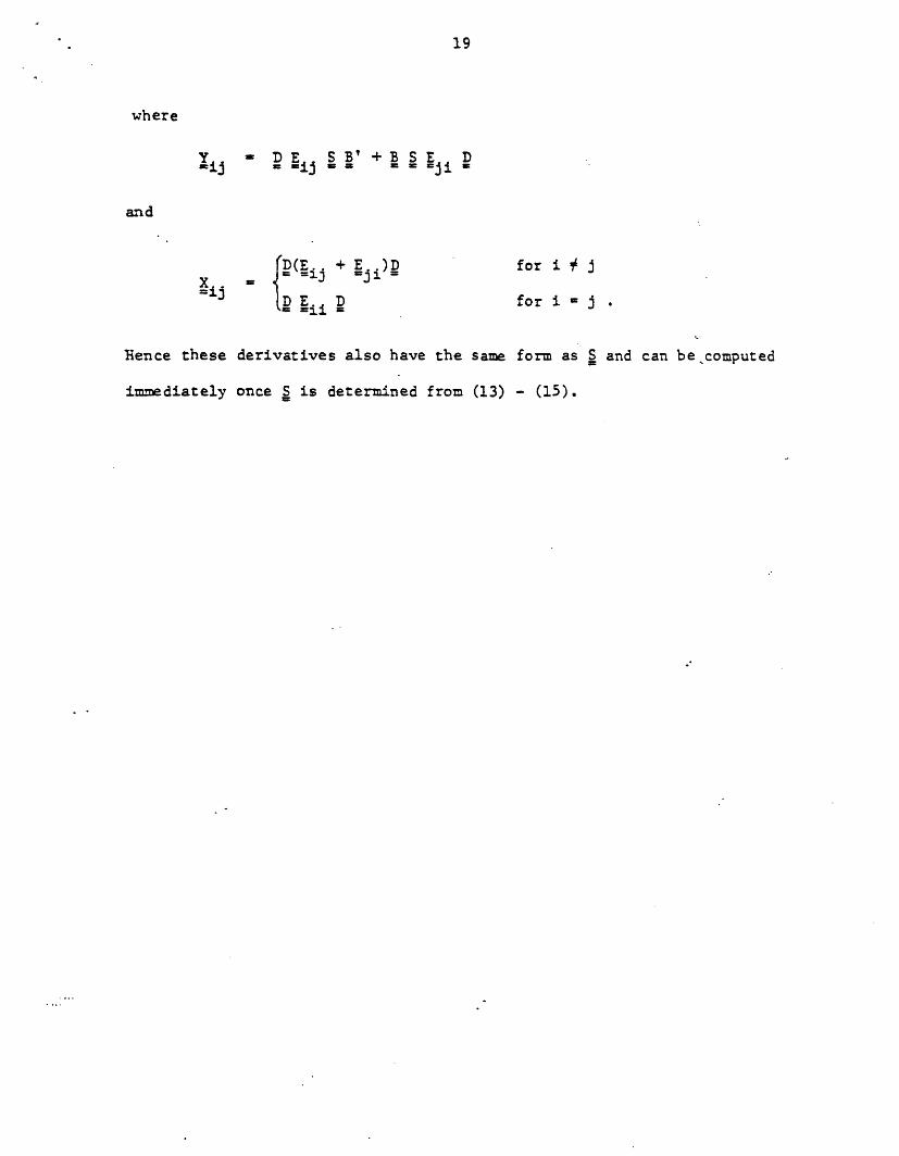
appropriate derivatives. We let S/Bak denote the matrix whose (i,j)

element is sij /a k . Then from (11) we find that

US x

(24)k B -=k BS kk s=O

where B is given in (11a) and

kZ = _[(^-I)SB' + D] + [BS((-'-I) + DP]EkkZk _kk [ ( k - ' +

where .. is a matrix of all zeroes except for a one in element (i,j).=i 3

We note that the infinite series in (24) is the same as that in (11),

except that Z is replaced by Z Hence we can find S/ak by the same=O

manner as we find S, but with ZO replaced by Zk. From this observation

it is easy to see that once we have found S [for instance,by performing

the diagonalization in (12)], we immediately can obtain S/'o k for

any k.

We may also have interest in changes to the covariance matrix S

with respect to changes in an element cij in the input/output matrix

and to changes in an element c.. in the covariance matrix for the noise

process, _. If we let S/Oij and CS/co.. denote these derivatives, then

we find that

I s cc"c- 5

=. ) B Y.. ce.. - = =j =ij s=O

and

ij s0 - = i=a s =0

1 Since the covariance matrix _ is necessarily symmetric we define the deri-

vative of S o be in terms of changes in both qij and .ji for i , j.

19

where

-ijEij S B'+BSE

=C =1 =C L =C =C =3± =

(D(E + E

x, - r ,D Eif 3

Hence these derivatives also have the same form as S and can be computed

immediately once S is determined from (13) - (15).

and

for i

for i - .

20

3. Example

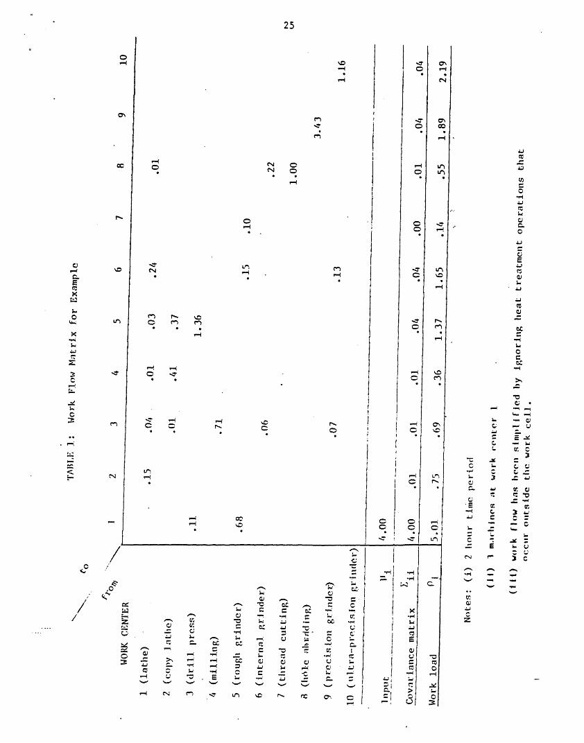
We illustrate the model here with a small example. The work flow

matrix is derived from a work cell at a factory that produces grinding machines.

The work cell fabricates several families of spindles that are components

in the assembly of the grinding machines. The work cell consists of ten

types of machining stations, and the work flow is described by the matrix

- given in Table 1. We note that the work flow matrix is quite sparse,

indicating that there are dominant flows through the work cell. In partic-

ular, all work enters the shop at the first work center (lathe) and then

moves serially through the shop but with some recycling. We remind the

reader that the work flow matrix is not a probability matrix but rather

its elements indicate the expected amount of work generated at a subsequent

station by a fixed amount of work at the current station. For example,

one hour of work at station 8 generates, on average, 3.43 hours of work

at station 9.

In addition to the matrix ¢ we need to specify the time period for he

model, the vector of expected inputs i and the covariance matrix . For

this example we set the nominal tize period to be two hours. Work enters

the shop only at station 1 and we assume that the expected input is four

hours of new work every time period (i.e., '1= 4, i = 0 i = 2, ...10).

We note that there are three identical lathes at work center 1 so an average

input of four hours of work each two hours is not obviously infeasible;

all other work stations have a single machine. We assume the noise process

{cit i normally distributed with its covariance matrix Z being a diage.a:

matrix as specified in Table 1. We note that most of the uncertainty is

introduced at the work center 1, presumably by the stream of new arrivals;

however, the arrival streams to the other work centers also are subject tc

a noise process, but with smaller variances.

21

Given and ~ we can compute the expected work load for each work

center,by (10). We report this in Table 1. We see that work centers 1, 6,

9 and 10 are the most heavily utilized centers. For a nominal time period

of two hours, the utilization at work center 1 is 83% since it consists of

three lathes. Work center 6 also has a utilization of 83%, and work center

9 has a utilization of 90%, while work center 10 has a utilization of 110%.

Indeed this analysis indicates that work center 10 need do, on average,

2.19 hours of work every two hours. This seems impossible given that there

is only one precision grinding machine available at this work center. Yet

this is what is required to meet the production requirements. Although

the model cannot prescribe how to meet this seemingly impossible requirement,

it does assist in identifying the necessary resource requirements. In par-

ticular, one might expect that this work center will work a ten-hour day

while all of the other work centers .work eight-hour days; hence, the effective

time period for work center 10 might actually be 2.5 hours rather than two

hours. The model should help to assess whether or not ten hours per day

is sufficient to cover the variability in these production requirements.

We are now ready to consider several different scenarios for managing

the flow of work through the shop. We specify a scenario by setting the

smoothing parameters ai. dr equivalently setting the planned lead times

n. = l/ci for each work station. For the first case we set the planned

lead time for each work station to be one period (ni = ); that is, at

each work station all work that arrives by the start of a time period is to

be processed by the end of that time period. Table 2 gives the characteriza-

tion of the shop behavior for this case. .-For each work center we report the

expected work load and its standard deviation, the expected queue at the

start of a period, and.the expected backlog at the start of a period. We

22

define the backlog at work center i to be the amount of the queue that has

been in queue at least n periods; but this is just the positive part of

Qm for == n, given by (20). From Table 2, we see that the work-in-

process levels are uite low and that there is never any backlog since

each work center clears its queue each time period. However, the production

requirements for each work center are highly variable. For instance, for

work center 1 the production requirement per time period has a normal

distribution with mean 5.01 hours and a standard deviation of 2.02 hours.

Hence, with probability .31 the production requirements for a time period

exceed the nominal production capacity of 6.00 hours, in which case

overtime would be worked or additional resources would be directed to this

work center. Similarly, we see that the other bottleneck work centers have

highly variable production requirements that will tend to result in ineffi-

cient production and high costs due to their lack of smoothness.

For the second case in Table 3 we attempt to smooth the production

recuirements at the heavily loaded work centers by imposing a planned queue.

We plan a ead time of four periods at work center 1, two periods at work

center 6, and three periods each at work centers 9 and i0. This results in

longer queues at these work centers as well as larger backlogs. For instance,

at work center , increasing the planned lead time from one to three time

periods triples the size of the queue. The expected backlog at work center

9 increases from zero to .13 hours; that is, on average the queue will contain

.13 hours of work that has been in queue for three or more time periods. Since

the average production per period at this work center is 1.89 hours, this

suggests that roughly 7% of the work takes longer than the planned lead time

of three time periods. (Due to the synmetry of the normal distribution,

a comparable aount of work, i.e., 7%, takes less than the planned lead

time of three time periods.) But the additional queues do result in signifi-

23

cant production smoothing as reflected in the smaller standard deviations

for production at the bottleneck work centers.

The third case reported in Table 4 is a continuation of the second

case in attempting to smooth the work flows. Again we have added queues

at the heavily loaded work centers to make their production requirements

less variable. But we begin to see here the effects of the decreasing

marginal benefits from additional smoothing. For instance, for ork center

6 increasing the planned lead time from one to two periods reduces its

production standard deviation by 56%, while increasing the planned lead

time from two to three periods gives only a 25% reduction in the production

standard deviation. (This is not an entirely fair comparison since the

reduction in the variability of the production requirements is not only

a consequence of the increased lead time at the work center, but also results

from the smoother arrival stream to that work center from the other work

centers).

The purpose of the fourth case (Table 5) is to show that we' can smooth

production not only by placing a cueue as a buffer at a work center, but also

by smoothing the arrival stream seen by the work center. We note from the

' matrix that work center 9 only receives work from work center 8. In the

previous two cases we try to smooth the work load at 9 by imposing a queue

there; ailternatively we could smooth the arrivals to work center 9 by

smoothing the production at 8. This is apparent not only from the above

reasoning, but also from computing the derivative of the variance of produc-

tion at work center 9 taken with respect to the smoothing parameters for

work center 8 [ecuation (24)]. I-n Table 5 we have increased the planned

lead time at work center 8 from one to two time periods; this results in

a smoother arrival stream to work center 9 that allows us to reduce its

planned lead time from .five to four time periods with no increase in its

24

production variability. Hence, we can begin to see how the control at one

work center impacts the work flow at another work center.

This example, as described by the four cases, illustrates a type of

analysis that one would do with the model. The analysis, as presented,

allows one to explore for a given shop configuration the tradeoff between

short flow times and low work-in-process inventory versus smooth production

and efficient allocation of production resources. As we have seen, attempting

to smooth production results in longer queues, and longer and more variable

flow times. Similarly, attempts to prune work-in-process or to speed up

the work flow will lead to more variable production requirements, if we

assume all else is unchanged. We have not prescribed a formal mechanism

for doing this exploration, although we have found reference to the deriva-

tive matrices {iS to be most helpful in guiding the search.

The model framework should also be helpful in doing other types

of analyses. In particular, we could examine a variety of "what if"

questions: lWhat if we had more/less capacity at various work centers? that

if the job mix or flow structure changes? What if we had better control

over the input stream to the shop so that the arrivals were less uncertain?

What if through improved scheduling we could reduce the variability in the

work flows between work centers? indeed, we expect that the model can be

a valuable planning tool for designing and assessing control strategies under

a variety of envirom=ental conditions.

25

,-1

-

O

C ·0

,-I

I-i

IC r ,C C? rlL1j 0 * M

-4

0

-

0

00

C

ITC

-4C

oo *Ii

-) .- ..

-' 'C C:h CC C -:h ~ ~O C : _ C

U~~~~ , * r _ _~ CJ -. - C U

*-. U! 'C ) - -- C : * L _ C._4 C; C 'C - _ C.

4J V i _: V _ C

-u '? U c: r C Ch i>: < i-. CL; C) C) C) - -4 ~ .L I.L C: -)_ L -E - .- - C, J

01-4

or

E

I-C)

:0

CI.-:Z..:iL;:Z

0. , -* 1

en C -I

v

I-

u)

C-40E

CQJ

-,0O

m)

- cCo

!

U:Y-

A _

_ row

- - 0E U

rrc.

-~ - C

_;

_ it

r- _.

£ C; t

3 3 C_ q

d

_. _

_ _u

tz

014

/

c1--

C

-

-4

,.L.

Czz

..

3 -ciu7

1-

'-4

CC qcc

..

II

I

II

ifIIIII

Lri

ii

1 L

,. 4

26

TABLE 2: CASE A

plannedlead time

n

expectedproductionE(P)

standarddeviation

C(P)

Work Center

1

2

3

4

5

6

7

8

9

10

expectedqueueE(Q)

expectedbacklogE(Qn)

5.01

.75

.69

.36

1.37

1.65

.14

.55

1.89

2.19

2.02

.32

.19

.17

.39

.54

.04

.17

.61

.74

5.01

.75

.69

.36

1.37

1.65

.14

.55

1.89

2.19

0

0

0

0

0

0

0

0

0OTO

::

O

27

TABLE 3: CASE B

plannedlead time

n

expectedproduction

E(P)

standarddeviation

O(P)

Work Center

1

2

3

4

5

6

7

8

9

10

expectedqueueE(Q)

expectedbacklog

E(Q n )

4

1

1

1

1

5.01

.75

.69

.36

1.37

.80

.16

.15

.12

.32

2

1

20.04

.75

.69

.36

1.37

3.31

.14

.55

5.68

6.58

.71

0

0

0

0

.05

0

.13

.10

1.65

.14

.55

1.89

2.19

1

3

3

.24

.03

.13

.29

.31

· _ _ i · � · _

· _

28

TABLE 4: CASE C

plannedlead time

n

expectedprod iict ion

E(P)

standarddeviation

a(P)

expected expectedqueue

E (Q)backlog

E (Qn)

Work Center

1

2

3

4

5

6

7

8

9

10.96 .13

8

1

1

1

2

5.01

.75

.69

.36

1.37

.55

.13

.14

.11

.20

40.07

.75

.69

.36

2.74

1.05

0

0

0

.06

3

1

1

5

1.65

.14

.55

4.97

.14

.18

.02

.11

.221.89

.07

0

0

.18

.55

9.45

r

10 5 2.19 .23

29

TABLE 5: CASE D

plannedlead time"

n

expectedproduct ion

E(P)

standarddeviationa (P)

Work Center

1

2

3

4

5

6

7

8

9

10

expectedqueue

E(Q)

expectedbacklogE(Qn)

5.01

.75

.69

. 36

1.37

1.65

.14

.55

1.89

2.19

.55

.13

.14

.11

.20

.18

.02

.08

.22

.23

40.07

.75

.69

.36

2.74

4.97

.14

1.10

7.56

10.96

1.05

'O

0

.06

.07

O

.02

.12

.13

_ __

__

--1�-11----·��1�.1 1_·111. __1_1111_�.1_1__� _1___�·._

30

4. Discussion

In this section-we review and discuss the key assumptions of the

proposed model. We also indicate in what directions we may extend the

basic model, as well as suggest issues in need of further investigation.

The most controversial assumption is likely to be the control rule

given by (1). In particular, we assume that there are no constraints on

setting the production levels in each time period. We suggest that one

set the control parameters (i.e. planned lead times) so that the produc-

tion requirements rarely exceed the normal range of production capacity.

Yet we do not explicitly constrain the production requirements to

do so, but argue that when the requirements exceed the normal capacity,

we can still satisfy the requirements (at a cost) by redeploying resources.

In some situations one might not be able to do this; in these instances,

we might have a rigid constraint so that we need restate the control rule

(1) as

it = miniQit,' it}

where Pit is the production capacity at work center i in time period t.

Although we have not tested this control rule in the context of a network

of queues, Cruickshanks et a. (19S4) have studied an analogous rule i. a

simpler setting consisting of one production stage. They find that the

study of the unconstrainted control rule [i.e. (1)] provides a reasoa:e

prediction of the behavior of the constrained control rule. We need tc

investigate, presu-mably by a simulation study, whether this observaticn

holds in the more complex setting of a hetwork of queues.

A second critical assumption is the Markov assumption made in (5).

We assume that it is possible to odel the work flows between work centers

in a Markov fashion so that the history of a work flow is not necessary.

31

In general it is hard to imagine how this assumption might be overcome

without resorting to a much more complex model structure. However, one

might relax the assumption that all jobs are of the same type and are

modelable by a single _ matrix. If there are a few distinct types of

jobs with different routings and production requirements, then one

might identify a work flow matrix (k) for each job type k so that its

work flow could be modeled separately. Each work center would have a

queue of work for each part type,and we would need a control rule that

set the production level as a function of the multiple queues; for instance,

we might restate (1) as

ikt tik Qikt

and

Pit = I Piktk

where Qikt is the queue of work for jobs of type k at work center i,

aik is the corresponding smoothing parameter, and Pikt is production

of jobs of type k at work center i. This extension would more faithfully

model the work flows when it is possible to identify distinct types of

jobs.

We have developed the model in the context of a job shop in which

work "pushes" its way through the system. Each work center has a queue

of work from which it sets its production level; the work center then

pushes its queue of work to the queues of downstream work centers, as

specified by the work flow matrix . In contrast to this we could conceive

of a shop in which work "pulls" its way through the shop. After each

work center is an inventory of work that has completed processing at

32

that work center; production is triggered by demand on this inventory, which

creates a backlog to be replenished. In other words, production at the

work center acts to fill the backlog by replenishing the inventory. Further-

more, production at the work center will pull inputs from the inventories

of upstream work centers, as specified by a work flow matrix. Such a

pull system is a mirror image of the job shop (push system) that we have

used to develop the model. We can apply the model directly to 'this system

by equating the queue (push) to the backlog (pull), and by defining the

(_ matrix to reflect how inputs are pulled into each work center.

Finally, the model may also be valuable for supporting the application

of a Materials Requirements Planning (MRP) system [Orlicky (1975)] in a

multi-stage or multi-plant production environment. The fundamental

construct of an MURP system is the notion of a planned lead time. Associated

with each production activity or stage is a lead time that forms the basis

for production pla-ning and materialprocurement. These lead times are

the primary control mechanisms for deciding when to order raw materials,

when to initiate part production and when to schedule subassemblies and

final assentlies in order to satisfy a given set of demand requirements.

Yet in the NaP literature I know of no theory on how to set these lead

times. What one often hears is that the planned lead times should be set

based on experience and observation; for instance, if we observe that the

actual lead tiAes for a production activity often exceed the planned

lead time, ten we need increase the planned lead time. But it is not

at all clear h;; much to increase the planned lead time or even if this

is the proper response. Indeed, one can argue that planned lead times

beyond a poin-. are just self-fulfilling prophecies; if I plan on an

activity to :ta:e, say, ten weeks, then I will load the activity with

work ten weeks before it is due and not surprisingly, it will take ten

33

weeks (or more if something goes wrong) before the work passes through the

activity. hat one needs is a normative model that could help to assess

the proper lead times for a given production system. It would seem that

the model proposed in this paper could be directly extended to the MRP

environment and would be of value in setting these planned lead times.

34

APPENDIX

We show here that the power series in (10) and in (11) will converge

if and only if the spectral radius (maximal absolute eigen value) of b

is less than one.

In order for the power series in (10) to converge we need

(Al) (I - D + D )s - .+

as s goes to infinity where 0 is the matrix of zeroes. But this is equi-

valent to requiring that the spectral radius of (I - D + D) be less than

one (Noble 1969). We will show that this will be true if and only if the

spectral radius of * is less than one. To do this we will use results from

the Frobenius theory of positive matrices (e.g. Karlin and Taylor, 1975,

pp. 542-551).

Let P(A) denoe the spectral radius of matrix A. Assume that p(C) < 1.

Suppose that C(I - D + D ) > 1 and let o and xc be the maximal absolute

eigen value and corresponding eigen vector for I - D + D ¢. That is

(I - D + D )x = X, x

But this can be rewritten as

x = xc + (o - 1) D xThus if > e that

Thus if to > l we have that

tx > - - o

IlI

35

since D is a positive matrix. But this contradicts the assumption that

p(=) < 1. Hence, if p(¢) < 1 we must have

o(I - D + D) <

Assume that p(O) > 1 and let u and x be the maximal absolute eigen· -- e-

value and corresponding eigen vector for =. Consider

(I - + D )x = ( -P)xo + X,

=xo + (X 0 - 1)D x

Thus if )X > 1 we have that

(I - D + D )x > ,

since D is a positive matrix. But this implies that p(I - D + D ) > 1.

Hence, if D(¢) > 1, then we must have that

p(I - D + D ) > 1

This completes the proof showing that (10) converges iff (.) <.

We now argue that (11) converges iff p(t) < 1. First,if (Al) is nc:

true, then it is easy to see that the series in (11) cannot converge. Second,

if (Al) is true, then we can show that :he series is absolutely convergent

(and thus convergent) by using (10) and (Al) to bound the corresponding series

of absolute values term by term.

III

36

REFERENCES

BERTRAND, J.W.M. AD J.C. WORTMANIN, Production Control and Information

Systems for Component Manufacturing Shops, Elsevier Science Publishing

Co., Amsterdam (1981).

BERTRAND, J.W.M., "The Effect of Workload Control on Order Flow Times",

in Operational Research '81, J. P. Brans (editor), North Holland

Publishing Co., (1981)..

CRUICKSHANKS, .B., R.D. DRESCHER AND S.C. GRAVES, "A Study of Production

Smoothing in a Job Shop Environment", Management Science, Vol, 30, No. 3,

(March 1984), pp. 368-380.

CONWAY, R.W., W.L. MXUELL AND L.W. MILLER, Theory of Scheduling ,

Addison-Wesley Publishing Co., Reading, MA, (1967).

GOMERS.ALL, E.R., "he Backlog Syndrome", Harvard Business Review,

Vol. 92, No. 5 (1964), 105-115.

HOLSTEIN, W.K. A- W.L. BERRY, "Work Flow Structure: An Analysis for

Planning ad Ccntrol", Management Science, Vol. 16, No. 6 (February 1970),

B-32L-B-336.

HOLSTEIN, W.K. and W.L. BERRY, "The Labor Assignment Decision: An Application

of Work Flc- Structure Information", Management Science, Vol. 18, No. 7

(March 1972), 90-400.

JACKSON, J.R., "etwcrks of Waiting Lines",Ooerations Research, Vol. 5

(1957), 518-521.

JACKSON, J.R., "Jobshop-Like Queueing Systems", Management Science,

Vol, 10 (1963), 131-142.

37

REFERENCES (Contd.)

JONES, C.H., "An Economic Evaluation of Job Shop Dispatching Rules",

Management Science,Vol..20 (1973), 293-307.

KARLIN, S. AND H.M. TAYLOR, A First Course in Stochastic Processes,

second edition, Academic Press, New York, (1975).

KARMARKAR, U. S., 1983, "Lot Size, Manufacturing Lead Times and"'

Utilization," Graduate School of Management Working Paper

(No. QM8312), University of Rochester.

NOBLE, B., Applied Linear Algebra, Prentice Hall, Inc., Englewood Cliffs,

New Jersey, (1969).

ORLICKY, J., Material Requirements Planning, McGraw-Hill, New York,

(1975).

IWIGHT, O., "InDut/Output Control - A Real Handle on Lead Time"

Production & Inventory Management, 3rd Qrt., (1970).

ZIPKIN, P. H., 1983, "Models for the Design and Control of

Stochastic, Multi-Item Batch Production Systems," Graduate School

Business Working Paper (No. 496A), Columbia University.

a �__