Embed Size (px)
Citation preview

Ministry of Education and Science of Ukraine
National Technical University Ukraine
"Igor Sikorsky Kiev Polytechnic Institute"
OPERATION CALCULATION Didactic material for a modal reference work on mathematical analysis for students
of 2nd year engineering faculties
Compilers: Zaderey Nadiya, Candidate of physico-mathematical sciences,
associate professor
Mamsa Kateryna, Candidate of physico-mathematical sciences, associate
professor
Nefodova Galyna, Candidate of physico-mathematical sciences
Perestyuk Mariya, Candidate of physico-mathematical sciences,
Director of EQMI NTUU “Igor Sikorsky KPI”
Kiev 2016
2
OPERATION CALCULATION
Didactic material for a modal reference work on mathematical analysis for students
of 2nd year engineering faculties / Compilers: Zaderey Nadiya, Mamsa Kateryna,
Nefodova Galyna, Perestyuk Mariya. – К., NTUU “Igor Sikorsky КPI”, 2016 – p. 40
Under the heading of scientist council of PМD NTUU “Igor Sikorsky КPI”
(Physics - Mathematics Department)
Educational publications
Under edition of compilers
The electronic version
Executive editor Y. P. Butsenko, Candidate of physico-mathematical sciences,
associate professor
Reviewer A.M. Kulik, Candidate of physico-mathematical sciences, associate
professor
Kiev 2016
3
Operational calculus.
Control work.
Introduction
Operational calculus is studied in the course of mathematical analysis in the third
semester. Surgery (symbolic) calculus widely used in various fields of science and
technology. A particularly important role it plays in the study of transients in linear
physical systems theory of electrical circuits, automation, radio engineering,
mechanics.
Didactic material contains 30 variants of modular control work being done by the
second year students of technical specialties in the third semester. The work consists
of five tasks and is designed for 90 minutes.
In the first task, you find the present original image. It helps to learn the definition of
the Laplace transform and its properties. The second task of the present must Find
image of the original. In the third task, you solve the Cauchy problem for linear
differential equations with piecewise continuous right-hand side. The fourth task is
proposed to solve the Cauchy problem for linear differential equations using
Duhamel integral. In the fifth task proposed Volterra integral equation of convolution
type. Each version of the control module attached reply.

4
The use of of operational calculations
I. Solution of Cauchy problem for linear differential equation with constant
coefficients in finding the right part of image
According to the plan:
1. By means of Laplace transformations upgrade linear differential equation in
relative algebraic image
2. Find out in this algebraic equation of the desired image of the original (called
operational solution)
3. According to reproduce the original image (answer)
Example 1 y"+2y'+y = sint y(0)=0, y'(0) = -1
y(t)Y(p)
y'(t)pY(p) – y(0) = pY(p) - 0 = pY(p)
y"(t)p2 Y(p) – py(0) - y'(0) = p
2Y(p)+1
sint 1
12 p
have the operator equation
p2Y(p)+1+2pY(p)+Y(p) = 1
12 p
Y(p)(p2+2p+1) = -1+ 1
12 p
Y(p) = - +
)1()1(
122 pp
(operational solution)
Find the original:
а) - 2)1(
1
p = )1
1(
p -te-t
applied the theorem of differentiation of the original
F'(p) -tf(t)
We have F(p)= 1
1
p e-t
b) relative to the second term we apply the second theorem of decomposition
)1()1(
122 pp
= ))(()1(
12 ipipp
P1= -i Pole of ІІ order
P2= -і simple pole
P3= i simple pole
F(p) = )1()1(
122 pp =
1ppres
F(p)ept
+2pp
res
F(p)ept
+3pp
res
F(p)ept
=
=limp
-1 )1
()!12(
12
p
e
dp
d pt
+limp
i)()1( 2 ipp
e pt
+limp
-i
)()1( 2 ipp
e pt
=
5
=limp
-122
2
)1(
2)1(
p
pepte ptpt
+2)1(2 ii
eit
+2)1(2
ii
e it
=
4
22 tt ete
ii
e it
22 +
)2(2 ii
e it
=
=
22
1
2
1
2
1 itittt ee
ete tete tt cos2
1
2
1
2
1
as the solution of a linear differential equation is a function of:
y(t) = -t te + tete tt cos2
1
2
1
2
1 = )cos(
2
1ttee tt
Example 2
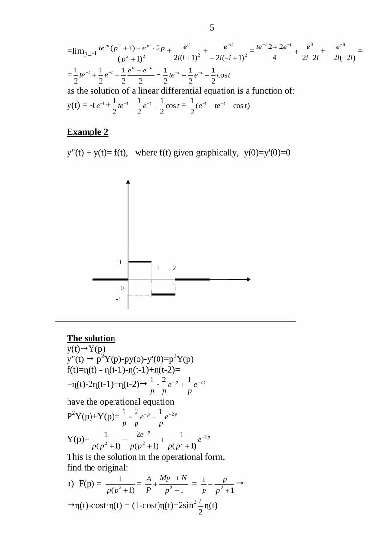
y"(t) + y(t)= f(t), where f(t) given graphically, y(0)=y'(0)=0
The solution
y(t)Y(p)
y"(t) p2Y(p)-py(o)-y'(0)=p
2Y(p)
f(t)=ɳ(t) - ɳ(t-1)-ɳ(t-1)+ɳ(t-2)=
=ɳ(t)-2ɳ(t-1)+ɳ(t-2)p
1- pp e
pe
p
212
have the operational equation
P2Y(p)+Y(p)=
p
1- pp e
pe
p
212
Y(p)= pp
epppp
e
pp
2
222 )1(
1
)1(
2
)1(
1
This is the solution in the operational form,
find the original:
а) F(p) = )1(
12 pp
= 12
p
NMp
P
A =
1
12
p
p
p
ɳ(t)-cost·ɳ(t) = (1-cost)ɳ(t)=2sin2
2
tɳ(t)
1 2 1
0
-1

6
b) Availability multipliers е-pa
points to the possibility of applying theorem of
delay:
е-pa
F(p)f(t-a)·ɳ(t-a)
because
pepp
)1(
22
2
1sin4 2 t
·ɳ(t-1)
pepp
2
2 )1(
1
2
2sin2 2 t
·ɳ(t-2)
Answer:
y(t) = 2sin2
2
t
·ɳ(t) – 2
1sin4 2 t
·ɳ(t-1) +2
2sin2 2 t
·ɳ(t-2)
Note: function y (t) will satisfy the equation at all points where it is continuous.
ІІ. The solution of the Cauchy problem without finding image of the right
side
Example 3
y"(t) = 21
1
t y(0)=y'(0)=0
The solution
If 21
1
tF(p) ( where F(p) – (some unknown images)
Then the operational equation is:
p2Y(p)=F(p)
Y(p)=2
1
pF(p) – operational solution
Operator solution got as a product of two images, by Borel theorem we have:
G(p)·F(p)g(t)*f(t)
We have G(p)= 2
1
pt , F(p)
21
1
t, so
Y(p)=2
1
p·F(p)=G(p)·F(p)g(t)*f(t)=
=
dtt
tdftg
tt
2
00
2 1
1)(
1
1*)()(
t
o
dt
21
-
-
td
0
21
= tarctg /0
t - )1ln(
2
1 2 /0
t= )()1ln(
2
1 2 tyttarctgt
Answer: y(t)=arctgt - )1ln(2
1 2t
Note:
1. The requirement of setting the initial conditions at the point t = 0 is not
essential, as the linear change of variables y = (-a new variable) Cauchy problem
at t = t0 ≠ 0 is reduced to the Cauchy problem with initial conditions at the point.
2. Similarly, the replacement of unknown function problem with nonzero initial
conditions can be reduced to a problem with zero initial conditions.
For example, if the initial conditions y(0)=y0 y'(0)=y1
then the replacement of the function y (t) to z (t), where z (t)

7
= y(t) – y0 –– y1t
we obtain:z(0) = 0
z'(0) = y'(t) – y1 / 0t= 0
3. If the initial conditions y0, y1, y2, yn-1 is not considered a given, but arbitrary
constants, then y (t) is not a solution of the Cauchy problem it is the general
solution of the differential equation.
ІІІ. Solving systems of linear differential equations with constant coefficients.
Systems of linear differential equations are solved similarly, the difference is that
we obtain a system of operational equations.
Example 4 x'=x+3y x=x(t) Initial conditions
y'=x–y y=y(t) x(0)=1, y(0)=0
The solution
x(t)X(p) x'(t)pX(p)-x(0)=pX(p)-1
y(t)Y(p) y'(t)pY(p)-y(0)=pY(p)
The system of operational equations:
pX(p)-1=X(p)+3Y(p)
pY(p)=X(p)-Y(p)
rewrite the system:
(p-1)X– 3Y=1 Х=
x
Х-(p+1)Y=0 Y=
y
p-1 -3 = -( 2p -1)+3 = - )4( 2 p
1 -(p+1)
1 -3
0 -(p+1) = -(p+1)
p-1 1 = -1
1 0
X=
x=
4
1
44
1222
pp
p
p
pch2t+ tsh2
2
1
Y=
y=
4
2
2
1
4
122
pp
tsh22
1
Answer: x(t)=ch2t+ tsh22
1
y(t)= tsh22
1
IV. The solution of integral equations Voltaire of the I and ІІ order
Integral equation is called the equation that contains the required function under
the integral sign.

8
Consider a simple integral equations of Voltaire wich type is convolution
І kind:
t
tfdytk0
)()()(
ІІ kind: y(t)+
t
tfdytk0
)()()(
where y (t) - desired function
f (t) - known function
k (t-) - known function, called the nucleus, and depend on the difference of
arguments.
If the function k (t-), f (t) are functions - originals, then using operational calculations
can find the solution of the integral equation.
let y(t)Y(p)
f(t)F(p)
k(t- )K(p)
then in operational form of the first equation isK(p)·Y(p) =F(p)
Y(p) = )(
)(
pK
pFy(t)
The second equation:Y(p)+K(p) ·Y(p) = F(p)
Y(p)=)(1
)(
pK
pF
y(t)
In both cases used the theorem of Borel about image convolution of two functions.
Example 5
y(x) = sinx+
x
dttytx0
)()( integral equation of the II kind
Y(p) = )(1
1
122
pYpp
Y(p) = )1
1
1
1(
2
1
)1)(1( 2222
2
pppp
p xxshx ),sin(
2
10
Answer: y(x)= xxshx ),sin(2
10
Example 6
t
tdyt0
sin)()cos( integral equation of the I kind
cost*y(t) = sint
12 p
p·Y(p) =
1
12 p
Y(p)=p
1 1
Answer: y(t)=1, t> 0

9
The structure of short-term module control work SCW – 3
1. Find the Laplace transform of the function - the original
2. Find image of the original data by Laplace
Solve linear differential equation with operational method
(45 minutes)
Structure of Module control work МCW – 3 1. Find the Laplace transform of the function - the original
2. Find image of the original data by Laplace
3. Solve the Cauchy problem for linear differential equations by operational
method
4. Solve the Cauchy problem for a linear differential equation using Duhamel
formula
5. To solve the integral equation of convolution operational method
(90 minutes)
For example:
1. f(t)=sin23t·e
2t= te
t 2
2
6cos1
)
36)2(
2
2
1(
2
12
p
p
p
2. F(p) = 4)1(
1
4)1(
1
4)1(
11
52 2222
pp
p
p
p
pp
p tete tt 2sin
2
12cos
3.y"+9y=ɳ(t-5)
y(0) = y'(0) = 0
p2Y(p) + 9Y(p)= pe
p
51
Y(p) = )9
1(
9
1
)9(
12
55
2
p
p
pee
pp
pp
так як 9
12
p
p
p
2
3sin23cos1 2 t
t
y(t) = )5(2
)5(3sin
9
2 2
tt
4. Find an image graphically of a given function f (t)
f(t) = ɳ(t-1) - ɳ(t-3) + (-t+4)ɳ(t-3) – (-t+4)ɳ(t-4)=
= ɳ(t-1)-(t-3)ɳ(t-3)-(t-4)ɳ(t-4)
ppp e
pe
pe
p
4
2
3
2
111
1
1
1 2 0 3 1 4

10
Example and solution of the problem «operator calculus».
1. Find the image function.
4 5cos 5 5
tf t e t t
2. Find original of the following image
2
3
4
pF p
p
3. Solve the Cauchy problem by operational calculations
2 , 0 0 0,
1, 0 1
0, 1
y y y f t y y
tf t
t
4. Using the formula Duhamel solve the solution of equation.
2
2 , 0 0 01
tey y y y y
t
5. Solve the integral equation
0
cos2
t
ty t e y d t
Exercise 1. Solving.
As you know 2
cos1
pt
p
, namely
2cos
1
pt t
p
. Because shift theorem:
4
2
4cos
4 1
t pe t t
p
, because lag theorem
4 5 5
2
4cos 5 5
4 1
t ppe t t e
p
.
Answer:
5
2
4
4 1
ppF p e
p
.
Exercise 2. Solving.
We know that 2
24
pch t
p
, by virtue of linear property,
2
33 2
4
pch t
p
.
Answer: 2
3
4
pF p
p
.
Exercise 3. Solving.
The right side of equation f t is piecewise continuous function. We write its
analytical expression:

11
1f t t t . By using the linearity property and applying lag theorem
1 1 pf t ep p
.
Let y t Y p . Then y t pY p , 2y t p Y p .
Let us write the operator equation
2 1 12 pp Y p pY p Y p e
p p
, where
2 2
1 1
1 1
pY p ep p p p
. We found
the original of the image. For table image have: 1
1
tep
.
By the image differencing theoreme we have
2 2
1 1 1
1 1 1
t t tte te tep p p
. By the integration of original
theorem:
2
0
11
1
t
t te d e tep p
. Therefore
2
11
1
t te te tp p
. Account for
lag theorem we obtain
1 1
2
11 1 1
1
t tpe e t e tp p
.
Answer: 1 11 1 1 1
t tt ty t e te t e t e t .
Exercise 4. Solving.
Find a solution 1y t subsidiary equation 2 1y y y by initial condition
0 0 0y y .
Let 1 1y t Y p . Then 2
1 1 1 1,y t pY p y t p Y p . Since 1
1p
, we get operator
equation: 2
1 1 1
12p Y p pY p Y p
p , from here
1 2
1
1Y p
p p
.
With the resulting image we find the original. This can be done in different ways.
First way. By expansion theorem
2
1 1 1 2 20 10 1
1lim lim
1 1
ptptpt pt
p pp p
e pe py t res y t e res y t e
p p p p

12
121
2
2 2
2
2 2
0 0
2
2
0 0
1 lim
11
1
1 1 1 1
11 1
1ln 1
21 1
1ln 1
21
pt ptt t t t
p
t t t
t t
t t t
t t
t t t
t
te p ey t e e te te
p
te te ep p
p pp p p
e ty t t e d e d e t arctgt t
ey t t e d e e t arctgt t
y t e t
2
0
1ln 1
2t
t t
arctgt t
e y d e y t
.
Second way.
Table image should:
2
1
1
ttep
. By the theorem of original integration we get
2
0
11
1
t
t te d te ep p
.
Third way.
Decompose proper rational fraction into a sum of simple fractions:
2 2
1 1 1 1
11 1p pp p p
.
From table images we obtain
2
11
1
t tte ep p
. Since 1 1 t ty t te e .
We have 1
t t t ty t e e te te . By Duhamel formula: 1
0
t
y t f y d .
Since, 2
2 2
0 0
1ln 1
21 1
t t
t t te ty t t e d e d e t arctgt t
.
Ansver: 21ln 1
2
ty t e t arctgt t
.
Exercise 5. Solving.
Considering that 0
( )
t
te y d
is convolution function te and y t .
Let y t Y p . Table image should: 1
1
tep
, 2
cos 24
pt
p
, by Borel theorem
1
tY p
e y tp
. So that, operator equation is written as:

13
21 4
Y p pY p
p p
, and its solution
2
1
4
pY p
p
can be represented as
2 2 2 2
1 1 2
24 4 4 4
p pY p
p p p p
. From the table we Find image of the original
1
cos2 sin 22
y t t t .
Answer: 1
cos2 sin22
y t t t .

14
Variant 1
1. Find image of the original 2 2sinte t
f tt
.
2. Find original of the following image
2
2 1
2
pF p
p
.
3. Solve the Cauchy problem by operational calculations
4 , 0 0 0,y y f t y y де
, 0 1
2 , 1 2
0, 2
t t
f t t t
t
.
4. Using the integral Duhamel solve the Cauchy problem
, 0 0 0y y tht y y .
5. Solve the integral equation 0
sin 1 cos
t
y t d t .
Variant 2
1. Find image of the original 4 5cos 5 5
tf t e t t
.
2. Find original of the following image 2
3
4
pF p
p
.
3. Solve the Cauchy problem by operational calculations
2 , 0 0 0,y y y f t y y де 1, 0 1
0, 1
tf t
t
.
4. Using the integral Duhamel solve the Cauchy problem
22 ,
1
tey y y
t
0 0 0y y .
5. Solve the integral equation 0
cos2
t
ty t e y d t .

15
Variant 3
1. Find image of the original sin5f t t t .
2. Find original of the following image 3 2
5 4 3
2 1
2
p p pF p
p p p
.
3. Solve the Cauchy problem by operational calculations
2 2 , 0 0 0,y y y f t y y де 1, 0 2
0, 2
tf t
t
.
4. Using the integral Duhamel solve the Cauchy problem
1,
1 ty y
e
0 0 0y y .
5. Solve the integral equation 3
2
03
tt
y t d
Variant 4
1. Find image of the original 4 cos2 cos5tf t e t t .
2. Find original of the following image 2 2
1
4 9F p
p p
.
3. Solve the Cauchy problem by operational calculations
4 , 0 0y y f t y де 3, 0 3
6, 3
tf t
t
.
4. Using the integral Duhamel solve the Cauchy problem
2 2 2 cos ,ty y y e t 0 0 0y y .
16
5. Solve the integral equation 0
sin
t
y t d y t t .
Variant 5
1. Find image of the original cos6 cos2t t
f tt
.
2. Find original of the following image 2
2 16
ppeF p
p
.
3. Solve the Cauchy problem by operational calculations
, 0 0y y f t y де 1, 0 2
0, 2
tf t
t
.
4. Using the integral Duhamel solve the Cauchy
problem 2 , 0 0 0y y th t y y .
5. Solve the integral equation 2
0
sin sin
t
y t d t .
Variant 6
1. Find image of the original 2sin t
f tt
.
2. Find original of the following image 2
1
4 1F p
p p
.
3. Solve the Cauchy problem by operational calculations
3 , 0 1y y f t y де 2, 0 1
1, 1
tf t
t
.
4. Using the integral Duhamel solve the Cauchy problem
1,y y
cht 0 0 0y y .

17
5. Solve the integral equation 2
0
cos
t
y t d t t .
Variant 7
1. Find image of the original sin7 sin3t t
f tt
.
2. Find original of the following image
2
1
1 1F p
p p
.
3. Solve the Cauchy problem by operational calculations
2 , 0 3y y f t y де 2, 0 1
1, 1
tf t
t
.
4. Using the integral Duhamel solve the Cauchy problem
,1
t
t
ey y
e
0 0 0y y .
5. Solve the integral equation 2
0
1
2
t
y t t t y d .
Variant 8
1. Find image of the original 0
t
f t sh d .
2. Find original of the following image 3
1
8F p
p
.
3. Solve the Cauchy problem by operational calculations
, 0 0 0y y f t y y де
1, 0 1
1, 1 2
0, 2
t
f t t
t
.

18
4. Using the integral Duhamel solve the Cauchy problem
2 ,1
tey y y
t
0 0 0y y .
5. Solve the integral equation 0
sin
t
y t y t d t .
Variant 9
1. Find image of the original 2 cos3f t sh t t .
2. Find original of the following image 2
3
4 3
pF p
p p p
.
3. Solve the Cauchy problem by operational calculations
, 0 0,y y f t y де 1, 0 2
0, 2
tf t
t
.
4. Using the integral Duhamel solve the Cauchy problem
1
, 0 03 t
y y ye
.
5. Solve the integral equation 0
cos
t
ty t t e y d .
Variant 10
1. Find image of the original 3cosf t t .
2. Find original of the following image 2 2
1
4 1F p
p p p
.

19
3. Solve the Cauchy problem by operational calculations
, 0 0 0,y y f t y y де
1, 0 1
1, 1 2
0, 2
t
f t t
t
.
4. Using the integral Duhamel solve the Cauchy problem
1,
1y y
cht
0 0 0y y .
5. Solve the integral equation 0
1 cos
t
y t t t y d .
Variant 11
1. Find image of the original 41 t
t
ef t
te
.
2. Find original of the following image 2 2( 2)
pF p
p
.
3. Solve the Cauchy problem by operational calculations
, 0 0 0,y y f t y y де
2, 0 1
1, 1 2
0, 2
t
f t t
t
.
4. Using the integral Duhamel solve the Cauchy problem
1,
1 ty y
e
0 0 0y y .
5. Solve the integral equation 2
02
ttt
y t t e d
.
Variant 12
1. Find image of the original 0
sint
f t d
.

20
2. Find original of the following image
3
1
peF p
p p
.
3. Solve the Cauchy problem by operational calculations
, 0 0 0,y y f t y y де 1 , 0 1
0, 1
t tf t
t
.
4. Using the integral Duhamel solve the Cauchy problem
3
14 ,
2y y
ch t 0 0 0y y .
5. Solve the integral equation 2
0
1
2
t
ty t e t y d .
Variant 13
1. Find image of the original 2 sin5f t sh t t .
2. Find original of the following image 2 2
1
1 ( 4)F p
p p p
.
3. Solve the Cauchy problem by operational calculations
4 , 0 0 0,y y f t y y де , 0 1
0, 1
t tf t
t
.
4. Using the integral Duhamel solve the Cauchy problem
2
1,y y
ch t 0 0 0y y .
5. Solve the integral equation 0
2 ( sin )
t
y t t t t y d .
Variant 14
1. Find image of the original sin 2 costf t e t t .

21
2. Find original of the following image
6
3 1
5
pF p
p
.
3. Solve the Cauchy problem by operational calculations
, 0 0 0,y y f t y y де
1, 0 1
2, 1 2
0, 2
t
f t t
t
.
4. Using the integral Duhamel solve the Cauchy problem
,1
t
t
ey y
e
0 0 0y y .
5. Solve the integral equation 0
sin 2 cos
t
y t t t y d .
Variant 15
1. Find image of the original 3 8tf t e t .
2. Find original of the following image
22
5 1
9
pF p
p
.
3. Solve the Cauchy problem by operational calculations
4 , 0 0 0,y y f t y y де
1, 0 1
1, 1 2
0, 2
t
f t t
t
.
4. Using the integral Duhamel solve the Cauchy problem
2
2 ,1
tey y y
t
0 0 0y y .
5. Solve the integral equation 0
11 sin
2
t
y t t y d .
Variant 16

22
1. Find image of the original 4 5cos 5 5
tf t e t t
.
2. Find original of the following image 2
2
5 6
pF p
p p
.
3. Solve the Cauchy problem by operational calculations
, 0 0 0,y y f t y y де
1, 0 1
1, 1 2
0, 2
t
f t t
t
.
4. Using the integral Duhamel solve the Cauchy problem
3
1,y y
ch t 0 0 0y y .
5. Solve the integral equation 0
2 cos
t
ty t e t y d .
Variant 17
1. Find image of the original 2 sin3f t ch t t .
2. Find original of the following image 2 2
1
1 ( 9)F p
p p
.
3. Solve the Cauchy problem by operational calculations
3 , 0 0 0,y y f t y y де 1, 0 4
0, 4
tf t
t
.
4. Using the integral Duhamel solve the Cauchy problem
2
2,
1
t
t
ey y
e
0 0 0y y .
5. Solve the integral equation 3
0
11
6
t
y t t y d .

23
Variant 18
1. Find image of the original sin 4f t t t .
2. Find original of the following image
2
21
peF p
p
.
3. Solve the Cauchy problem by operational calculations
, 0 0 0,y y f t y y де 1, 0 2
4, 2
tf t
t
.
4. Using the integral Duhamel solve the Cauchy problem
2 ,1
ttey y y
t
0 0 0y y .
5. Solve the integral equation 0
t
y t t sh t y d .
Variant 19
1. Find image of the original sinf t t t .
2. Find original of the following image 4 2
1
5 4F p
p p
.
3. Solve the Cauchy problem by operational calculations
4 , 0 0 0,y y f t y y де 1, 0
0,
tf t
t
.
4. Using the integral Duhamel solve the Cauchy problem
2
,2
t
t
ey y
e
0 0 0y y .
5. Solve the integral equation 0
t
y t sht ch t y d .

24
Variant 20
1. Find image of the original cos3f t sht t .
2. Find original of the following image 2
3
( 4 3)
pF p
p p p
.
3. Solve the Cauchy problem by operational calculations
9 , 0 0 0,y y f t y y де 0, 0 3
1, 3
tf t
t
.
4. Using the integral Duhamel solve the Cauchy problem
2,
shty y
ch t 0 0 0y y .
5. Solve the integral equation 0
sin
t
y t t t y d .
Variant 21
1. Find image of the original 2
0
sin
t
f t d .
2. Find original of the following image 3
1
( 1)F p
p p
.
3. Solve the Cauchy problem by operational calculations
4 , 0 0 0,y y f t y y де 0, 2
2, 2
tf t
t
.
4. Using the integral Duhamel solve the Cauchy problem
2,
( 1)
t
t
ey y
e
0 0 0y y .
5. Solve the integral equation 0
t
ty t t e y d .

25
Variant 22
1. Find image of the original 2 1 cos3f t t t .
2. Find original of the following image 2
1
( 1)F p
p p
.
3. Solve the Cauchy problem by operational calculations
2 , 0 0y y f t y де 2, 0 1
1, 1
tf t
t
.
4. Using the integral Duhamel solve the Cauchy problem
22 ,
1
tey y y
t
0 0 0y y .
5. Solve the integral equation 0
t
t ch t y d .
Variant 23
1. Find image of the original tf t t e cht .
2. Find original of the following image 2 2
1
( 1)F p
p
.
3. Solve the Cauchy problem by operational calculations
3 , 0 0 0,y y f t y y де 0, 2
1, 2
tf t
t
.
4. Using the integral Duhamel solve the Cauchy problem
22 ,
tey y y
ch t 0 0 0y y .
5. Solve the integral equation 0
t
y t t sh t y d .
26
Variant 24
1. Find image of the original 1 sin2f t t t .
2. Find original of the following image 3
3( 1)
peF p
p
.
3. Solve the Cauchy problem by operational calculations
3 , 0 0 0,y y f t y y де 0, 1
1, 1
tf t
t
.
4. Using the integral Duhamel solve the Cauchy problem
22 ,
tey y y
ch t
0 0 0y y .
5. Solve the integral equation 2
0
cos
t
t t t y d .
Variant 25
1. Find image of the original 2 3tf t t e .
2. Find original of the following image 2
1
7F p
p p
.
3. Solve the Cauchy problem by operational calculations
3 , 0 0y y f t y де
1, 0 1
1, 1 2
1, 2
t
f t t
t
.
4. Using the integral Duhamel solve the Cauchy problem
2 ,1
tey y y
t
0 0 0y y .
5. Solve the integral equation 0
t
y t sht t y d .

27
Variant 26
1. Find image of the original 2cosf t t t .
2. Find original of the following image 4
2
3
9
peF p
p
.
3. Solve the Cauchy problem by operational calculations
4 , 0 0 0,y y f t y y де 0, 2
2, 2
tf t
t
.
4. Using the integral Duhamel solve the Cauchy problem
1,
3ty y
e
0 0 0y y .
5. Solve the integral equation 0
1 2 cos
t
y t t y d .
Variant 27
1. Find image of the original 2
0
sin
t
f t t d .
2. Find original of the following image 2
2
peF p
p
.
3. Solve the Cauchy problem by operational calculations
2 , 0 3y y f t y де 2, 0 1
1, 1
tf t
t
.
4. Using the integral Duhamel solve the Cauchy problem
1,
1ty y
e
0 0 0y y .
5. Solve the integral equation 0
1 sin
t
y t t t y d .

28
Variant 28
1. Find image of the original 2 1 tf t t e .
2. Find original of the following image 3
2 3
1
pF p
p
.
3. Solve the Cauchy problem by operational calculations
, 0 0y y f t y де 1, 0 2
0, 2
tf t
t
.
4. Using the integral Duhamel solve the Cauchy problem
1,
1ty y
e
0 0 0y y .
5. Solve the integral equation 0
t
y t t t y d .
Variant 29
1. Find image of the original 2tf t te cht .
2. Find original of the following image 2
2
4
ppeF p
p
.
3. Solve the Cauchy problem by operational calculations
4 , 0 0y y f t y де 1, 0 3
2, 3
tf t
t
.
4. Using the integral Duhamel solve the Cauchy problem
,1
t
t
ey y
e
0 0 0y y .
5. Solve the integral equation 0
sin
t
y t t t y d .

29
Variant 30
1. Find image of the original 0
sin
t
f t e d .
2. Find original of the following image 3 2
1
2F p
p p p
.
3. Solve the Cauchy problem by operational calculations
, 0 0y y f t y де 1, 0 2
0, 2
tf t
t
.
4. Using the integral Duhamel solve the Cauchy problem
, 0 0 0y y tht y y .
5. Solve the integral equation 0
t
t ty t e e y d .
Answer:
Variant 1
1.
2
1 2ln
2 2 4
pF p
p
2. 2 22 5t tf t e te
3. 1 1 1 1 1 1
sin 2 1 sin 2 1 1 2 sin 2 2 24 2 2 2 4 2
y t t t t t t t t t t
4. 22
ty t sht cht arctg th
5. y t t
Variant 2
1.
5
2
4
4 1
pe pF p
p
2. 3 2f t ch t
3. 1 11 1 1 1
t tt ty t t e te t e t e

30
4. 21ln 1
2
ty t e t arctgt t
5. 1
cos2 sin 22
y t t t
Variant 3
1.
22
10
25
pF p
p
2. 21
2
tf t te t
3. 21 11 cos sin 1 cos 2 sin 2 2
2 2
tty t e t t t e t t t
4. 1 1 ln 2 1 ln 1t t t ty t e e t e e
5. y t t
Variant 4
1.
2 2
1 4 4
2 4 9 4 49
p pF p
p p
2. 1 1 1
sin 2 sin35 2 3
f t t t
3. 4 343 31 1 3
4 4
tty t e t e t
4. sinty t te t
5. 3 1
cos22 2
y t t
Variant 5
1. 2
2
1 4ln
2 36
pF p
p
2. cos4 2 2f t t t
3. 21 1 2
tty t e t e t

31
4. 2 24
ty t sht arctge cht
5. 3 1
cos22 2
y t t
Variant 6
1. 2 41
ln2
pF p
p
2. 2 21 1 1
3 4 12
t t tf t e e e
3. 3 132 11 1 1
3 3
tty t e t e t
4. lny t tsht cht cht
5. 2 3
1 22 3
t ty t t
Variant 7
1. 2
2
1 16ln
4 100
pF p
p
2. 2 1t tf t e e t
3. 2 12 2 13 1 1 1
2
tt ty t e t e t e t
4. 1
1 ln2
tt t e
y t te e
5. 2 21 3 3
cos 3 sin3 2 2
t t
ty t e e t e t
Variant 8
1. 2
1
1F p
p p
2. 21 1 1cos 3 sin 3
12 12 4 3
t t tf t e e t e t

32
3. 1 cos 2 1 cos 1 1 1 cos 2 2y t t t t t t t
4. ( 1 ln 1 )ty t e t t t
5. 31
6y t t t
Variant 9
1.
2 2
1 2 2
2 2 9 2 9
p pF p
p p
2. 31 2 t tf t e e
3. 21 1 2
tty t e t e t
4. 1 1 3
1 ln3 9 9 4
tt t tt e
y t e e e
5. 22 3 1cos sin
5 5 5
ty t e t t
Variant 10
1. 2 2
1 3
4 9 1
p pF p
p p
2. 1
3 4cos cos212
f t t t
3. 2 2 21 22 sin 2sin 1 sin 2
2 2 2
t t ty t t t t
4. 2 1
1 ln21t
chty t sht t cht
e
5. 23 3
2 cos 3sin2 2
t
y t t e t t
Variant 11
1. 5
ln | |1
pF p
p

33
2. sin 22 2
tf t t
3. 1 22 1 1 1 1 2 1 2
t tty t t e t t e t t e t
4. 1 1
1 ln2 2
tt t e
y t e te sht
5. 2 3
21 3 1
16 8 8 12 16
tt t ty t e
Variant 12
1. arcctg p
F pp
2. 33 3
tf t e t t
3. 1 cos sin ) 1 sin 1 1y t t t t t t t t t
4. 2 2
2
sh ty t
ch t
5. 21 1 1 3 3
cos 3sin2 6 3 2 2
t
t ty t e e e t t
Variant 13
1.
2 2
5 1 1
2 2 25 2 25F p
p p
2. 1 3 1
cos cos23 4 4
f t t t
3. 1 1 1 1 1
sin 2 1 sin 2 1 1 1 cos2 1 14 2 4 2 4
y t t t t t t t t t
4. 2 1ty t sht arctge cht
5. 1 2sin 2
3 2
t ty t e e t
Variant 14
34
1.
2 2
1 1 3
2 1 1 1 9F p
p p
2. 4 5 5 53 16
4! 5!
t tf t t e t e
3. 1 21 1 1 1 2 1 2 2t t ty t e t t e t t e t t
4. 1 1 1
ln2
t t t
t t
e e ey t
e e
5. ty t te
Variant 15
1.
9
8!
3F p
p
2. 5
sin36
tf t t
3. 4 1 4 241 1 1 1 1 1 1 22 1 2
16 16 4 16 16 16 16 16 16
t tt t t ty t e t e t e t
4.
2
2
21 ln 1
1
t tty t t e e t t
t
5. 14 cos 3
3y t t
Variant 16
1.
5
2
4
4 1
pe pF p
p
2. 2 34 5t tf t e e
3. 1 cos 2 1 cos 1 1 1 cos 2 2y t t t t t t t
4. 21 2
2
sh ty t
cht
5. ty t cht te
Variant 17

35
1.
2 2
3 1 1
2 2 9 2 9F p
p p
2. 1
cos cos38
f t t t
3. 1 11 cos 3 1 cos 3 4 4
3 3y t t t t t
4. 1 1
1 ln2 2
tt e
y t e
5. 1
cos2
y t cht t
Variant 18
1.
22
8
16
pF p
p
2. 22 2tf t t e t
3. 1 cos 3 1 cos 2 2y t t t t t
4. 2
( 1 ln 1 )2
t ty t e t t t
5. 3
6
ty t t
Variant 19
1. 2 1
peF p
p
2. 1 2
3 2
sh ty t sht
3. 1 1
1 cos2 1 cos24 4
y t t t t t
4. 2
2 ln 13
tt te
y t e e
5. 22 5
25
t
y t e sh t

36
Variant 20
1.
2 2
1 1 1
2 1 9 1 9
p pF p
p p
2. 31 2 t tf t e e
3. 1 1
3 cos3 3 39 9
y t t t t
4. 2
2 2
1 2 1 11 ln
21 1
tt
t t
ey t e tht
cht e e
5. 1 1
sin2 2
y t sht t
Variant 21
1. 2
2
4F p
p p
2. 2
12
t ty t e t
3. 1 1
2 cos2 2 22 2
y t t t t
4. 1
ln 11 1
t t
t t
chty t e e
e e
5. 2
2
ty t t
Variant 22
1.
2
2 22
2 9
99
p pF p
pp
2. 1 cosy t t
3. 2 12 11 1 1
2
tty t e t e t
4. 2( ln 1 )ty t e arctgt t
5. 2
12
ty t
37
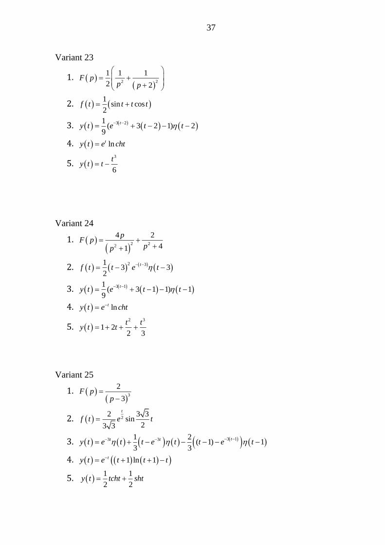
Variant 23
1.
2 2
1 1 1
2 2F p
p p
2. 1
sin cos2
f t t t t
3. 3 21( 3 2 1) 2
9
ty t e t t
4. lnty t e cht
5. 3
6
ty t t
Variant 24
1.
2 22
4 2
41
pF p
pp
2. 2 31
3 32
tf t t e t
3. 3 11( 3 1 1) 1
9
ty t e t t
4. lnty t e cht
5. 2 3
1 22 3
t ty t t
Variant 25
1.
3
2
3F p
p
2. 22 3 3
sin23 3
t
f t e t
3. 3 13 31 2( 1) 1
3 3
tt ty t e t t e t t e t
4. 1 ln 1ty t e t t t
5. 1 1
2 2y t tcht sht

38
Variant 26
1.
2
2 22
1 1 4
2 4
pF p
p p
2. sin3 4 4f t t t
3. 1 1
cos2 2 22 4
y t t t
4. 1 1 3
1 ln3 9 9 4
tt t tt e
y t e e e
5. 1 2 ty t te
Variant 27
1. 3 2
2 1
1F p
p p
2. 2 2f t t t
3. 2 12 11 1 1
2
tty t e t e t
4. 1 1
1 ln2 2
tt t e
y t e te sht
5. 2 3
12 6
t ty t t
Variant 28
1. 3
2 1
1( 1)F p
pp
2. 2 21 1 3 5 3
cos sin3 3 2 23
t t
tf t e e t e t
3. 21 1 2
tty t e t e t
4. 1 1 ln 2 1 ln 1t t t ty t e e t e e
5. siny t t
Variant 29

39
1.
2 2
1 1 1
2 3 1F p
p p
2. ( 2 1 ) 1f t ch t t
3. 4 341 1( 3) 3
4 4
tty t t e t t e t
4. 1
1 ln 12
tt te
y t e e
5. 2
12
ty t
Variant 30
1. 2
1
2F p
p p
2. 1 t tf t te e
3. 21 1 2
tty t e t e t
4. 22
ty t sht cht arctg th
5. 2ty t e
References
1. M.L.Krasnov, A.I.Kiselev, G.I.Makarenko. Functions of a complex
variable. Operational calculus. Stability theory. Moscow, "Science", 1981. -
300p.
2. Problems in Mathematics for Technical Schools. Special sections of
analiza.-V4ch. Part2. textbook (Edited A.V.Efimova, B.P.Demidovicha).
Moscow, "Science". 1981.-306p.

40
3. V.F.Chudesenko. Collection of tasks for special courses of higher
mathematics. (model calculations): Textbook for vtuzov.- M .: Higher.
School, 1983.-112p.
4. І.V.Alєksєєva, V.O.Gaydey, O.O.Dihovichny, L.B.Fedorova. Cooperate for.
Teorіya funktsіy kompleksnoї zmіnnoї. Operatsіyne numbers. Workshop.
Kiїv.- 2013, 160p.