Embed Size (px)
Citation preview

OpenSim
�
Evaluating an Open Source
Simulation Software
for Human Movements
Technical Report
Nicolas Schwenck
Department of Mechanics
Kungliga Tekniska Högskolan
Stockholm, July 2009


Preface
This thesis mainly results from my work at the Department of Mechanics from August till
December 2008.
I thank Professor Anders Eriksson who helped me to get in touch with the �eld of biomechanics
and gave me the opportunity to write this thesis at KTH and also for always o�ering me great
advice and support.
I thank Lanie Gutierrez-Farewik for the contact to the Karolinska University Hospital, for
supervising the work in the motion laboratory and the medical part guidance.
I thank Olesya for the very productive discussions and the corporate work in the motion labo-
ratory.
I thank Professor J.F. Wagner for the support at the University of Stuttgart.
I also would also like to thank my parents who have given me the �nancial possibility for staying
in Stockholm and who always have supported me.
iii


Abstract
The open source software OpenSim is a biomechanical simulation software. It was specially
developed at Stanford University for the analysis of human movements. Its functions were
analysed and tested by means of some examples. In this project the focus of the examples lays
in manipulating motions of the human gait.
Forward dynamic simulations were done by altering muscle excitation patterns and computing
the resulting motions. Backward dynamic simulations were done by scaling motions or creating
new movements, computing the needed muscle forces and excitations.
The compatibility to an important commercial software (SIMM) on which OpenSim is based
was tested.
This thesis consequently shows the feasibility of the methods mentioned above to manipulate
motions and its applicability to real cases and states the prospects of OpenSim in the �eld of
biomechanical simulation software for analysing human movements.
The test results show that OpenSim can ful�l the requirements within the small range of the
test cases. It also shows that some modules are not stable enough and that documentation
and the error message system have to be improved. The tests show that further veri�cation
and validation is necessary to con�rm the used algorithms. The usage as commercial software
replacement is not recommended at present, but it seems to be a cheap and useful alternative
for teaching purposes.
v


Contents
Preface iii
Abstract iv
Contents vi
List of Figures ix
1 Introduction 1
1.1 Biomechanics . . . . . . . . . . . . . . . . . . . . . . . . . . . . . . . . . . . . . . 1
1.2 Simulations of Human Movement . . . . . . . . . . . . . . . . . . . . . . . . . . . 1
1.2.1 Motion Laboratory . . . . . . . . . . . . . . . . . . . . . . . . . . . . . . . 2
1.3 OpenSim and SIMM . . . . . . . . . . . . . . . . . . . . . . . . . . . . . . . . . . 2
1.4 Outline of this Thesis . . . . . . . . . . . . . . . . . . . . . . . . . . . . . . . . . 3
2 Fundamentals 5
2.1 Multi Body Mechanics . . . . . . . . . . . . . . . . . . . . . . . . . . . . . . . . . 5
2.2 Numerics . . . . . . . . . . . . . . . . . . . . . . . . . . . . . . . . . . . . . . . . 6
2.2.1 Runge-Kutta . . . . . . . . . . . . . . . . . . . . . . . . . . . . . . . . . . 6
2.2.2 Optimisation . . . . . . . . . . . . . . . . . . . . . . . . . . . . . . . . . . 8
3 OpenSim 11
3.1 Example Operating Sequence . . . . . . . . . . . . . . . . . . . . . . . . . . . . . 11
3.1.1 Scaling . . . . . . . . . . . . . . . . . . . . . . . . . . . . . . . . . . . . . . 11
3.1.2 Inverse Kinematics . . . . . . . . . . . . . . . . . . . . . . . . . . . . . . . 11
3.1.3 Inverse Dynamics . . . . . . . . . . . . . . . . . . . . . . . . . . . . . . . . 12
3.1.4 Forward Dynamics and Analysis . . . . . . . . . . . . . . . . . . . . . . . 12
3.2 Muscle Force Computation . . . . . . . . . . . . . . . . . . . . . . . . . . . . . . 13
3.2.1 Correlation Between Muscle Force and Excitation Level . . . . . . . . . . 14
3.3 Special Features . . . . . . . . . . . . . . . . . . . . . . . . . . . . . . . . . . . . . 15
3.3.1 Residual Reducing Algorithm . . . . . . . . . . . . . . . . . . . . . . . . . 15
3.3.2 Computing Muscle Control . . . . . . . . . . . . . . . . . . . . . . . . . . 17
4 Results 19
4.1 Motion Laboratory results . . . . . . . . . . . . . . . . . . . . . . . . . . . . . . . 19
4.2 Manipulate Motions . . . . . . . . . . . . . . . . . . . . . . . . . . . . . . . . . . 21
4.2.1 Musculoskeletal Geometry . . . . . . . . . . . . . . . . . . . . . . . . . . . 22
vii

OpenSim - Open Source Simulation Software for Human Movements
4.2.2 Change Excitation Patterns . . . . . . . . . . . . . . . . . . . . . . . . . . 24
4.2.3 Scale Motions . . . . . . . . . . . . . . . . . . . . . . . . . . . . . . . . . . 26
4.2.4 Create New Motions . . . . . . . . . . . . . . . . . . . . . . . . . . . . . . 27
4.3 Compatibility to SIMM (Import/Export) . . . . . . . . . . . . . . . . . . . . . . 30
4.4 Conclusions . . . . . . . . . . . . . . . . . . . . . . . . . . . . . . . . . . . . . . . 32
5 Extension � Comparison v1.5.5 vs. v1.8.1 33
5.1 Optimisers . . . . . . . . . . . . . . . . . . . . . . . . . . . . . . . . . . . . . . . . 33
5.2 Compatibility to SIMM . . . . . . . . . . . . . . . . . . . . . . . . . . . . . . . . 34
5.3 Comparison of the User's Guides . . . . . . . . . . . . . . . . . . . . . . . . . . . 34
5.4 Stability . . . . . . . . . . . . . . . . . . . . . . . . . . . . . . . . . . . . . . . . . 34
5.4.1 RRA . . . . . . . . . . . . . . . . . . . . . . . . . . . . . . . . . . . . . . . 34
5.4.2 CMC . . . . . . . . . . . . . . . . . . . . . . . . . . . . . . . . . . . . . . . 35
5.4.3 Forward Dynamics . . . . . . . . . . . . . . . . . . . . . . . . . . . . . . . 35
5.5 Comparison of the Test Cases . . . . . . . . . . . . . . . . . . . . . . . . . . . . . 35
5.5.1 Change Excitation Patterns . . . . . . . . . . . . . . . . . . . . . . . . . . 35
5.5.2 Scale Motions . . . . . . . . . . . . . . . . . . . . . . . . . . . . . . . . . . 38
5.5.3 Create New Motions . . . . . . . . . . . . . . . . . . . . . . . . . . . . . . 40
5.6 Movements Without Ground Reactions . . . . . . . . . . . . . . . . . . . . . . . . 40
5.7 Project Proposal � CMC and NMT, Two Muscle Force Computation Approaches 41
5.7.1 Introduction . . . . . . . . . . . . . . . . . . . . . . . . . . . . . . . . . . . 41
5.7.2 Methods that Could Be Used . . . . . . . . . . . . . . . . . . . . . . . . . 42
5.7.3 Signi�cance of this Study . . . . . . . . . . . . . . . . . . . . . . . . . . . 42
6 Experiences and Future Work 43
6.1 Version 1.5.5 . . . . . . . . . . . . . . . . . . . . . . . . . . . . . . . . . . . . . . 43
6.2 Version 1.8.1 . . . . . . . . . . . . . . . . . . . . . . . . . . . . . . . . . . . . . . 45
Bibliography 47
A Appendix 51
A.1 Motion Laboratory . . . . . . . . . . . . . . . . . . . . . . . . . . . . . . . . . . . 52
A.1.1 Hip Flexion/Extension . . . . . . . . . . . . . . . . . . . . . . . . . . . . . 53
A.1.2 Hip Ab-/Adduction . . . . . . . . . . . . . . . . . . . . . . . . . . . . . . . 54
A.1.3 Hip Rotation . . . . . . . . . . . . . . . . . . . . . . . . . . . . . . . . . . 55
A.1.4 Knee Flexion/Extension . . . . . . . . . . . . . . . . . . . . . . . . . . . . 56
A.2.2 Change Excitation Patterns . . . . . . . . . . . . . . . . . . . . . . . . . . 57
A.2 Manipulate Motions . . . . . . . . . . . . . . . . . . . . . . . . . . . . . . . . . . 58
A.2.1 Musculoskeletal Geometry . . . . . . . . . . . . . . . . . . . . . . . . . . . 58
A.2.3 Scale Motions . . . . . . . . . . . . . . . . . . . . . . . . . . . . . . . . . . 59
A.2.4 Create New Motions . . . . . . . . . . . . . . . . . . . . . . . . . . . . . . 60
A.3 Extension . . . . . . . . . . . . . . . . . . . . . . . . . . . . . . . . . . . . . . . . 61
A.3.1 Change Excitation Patterns . . . . . . . . . . . . . . . . . . . . . . . . . . 61
A.3.2 Scale Motions . . . . . . . . . . . . . . . . . . . . . . . . . . . . . . . . . . 62
viii

OpenSim - Open Source Simulation Software for Human Movements
A.3.3 Movements Without Ground Reactions . . . . . . . . . . . . . . . . . . . . 63
A.4 Source Codes . . . . . . . . . . . . . . . . . . . . . . . . . . . . . . . . . . . . . . 64
A.4.1 Motion Laboratory . . . . . . . . . . . . . . . . . . . . . . . . . . . . . . . 64
A.4.2 Scale Motions . . . . . . . . . . . . . . . . . . . . . . . . . . . . . . . . . . 67
ix


List of Figures
3.1 Dimensionless model of muscle and tendon . . . . . . . . . . . . . . . . . . . . . . 14
4.1 Spatial coordinate system of the human body . . . . . . . . . . . . . . . . . . . . 20
4.2 Location of the body-segmental reference frames, the lower extremities . . . . . . 22
4.3 Location of the body-segmental reference frames, the foot . . . . . . . . . . . . . 23
4.4 Comparison of original and changed excitations of left knee �exors . . . . . . . . 25
4.5 Comparison of original and changed excitations of left knee extensors . . . . . . . 25
4.6 Left Knee Flexion/Extension . . . . . . . . . . . . . . . . . . . . . . . . . . . . . 26
4.7 Flexion/Extension of the right hip joint . . . . . . . . . . . . . . . . . . . . . . . 27
4.8 Comparison between CMC calculated excitation of right Gluteus Maximus . . . . 28
4.9 Comparison between CMC calculated excitation of right Psoas and Iliacus . . . . 28
4.10 Prescribed values for the hip/knee during the kick motion . . . . . . . . . . . . . 29
4.11 Position of the left foot and knee joint during the kick motion . . . . . . . . . . . 30
4.12 Summed main �exors/extensors muscle forces of the hip/knee during knee bending 31
4.13 Summed main �exors/extensors muscle forces of the hip/knee during a kick move-
ment . . . . . . . . . . . . . . . . . . . . . . . . . . . . . . . . . . . . . . . . . . . 31
5.1 Extension and �exion of the left and right knee and hip joint . . . . . . . . . . . 36
5.2 CMC calculated excitation of the Gastrocnemius . . . . . . . . . . . . . . . . . . 37
5.3 CMC calculated excitation of the Vastus Intermedius . . . . . . . . . . . . . . . . 37
5.4 Angle values for subtalar and ankle joint of the left leg during a Forward Dynamics
computation . . . . . . . . . . . . . . . . . . . . . . . . . . . . . . . . . . . . . . . 38
5.5 Flexion/Extension of the right hip joint . . . . . . . . . . . . . . . . . . . . . . . 39
5.6 Comparison between CMC calculated excitation of right Gluteus Maximus for a
longer period of time . . . . . . . . . . . . . . . . . . . . . . . . . . . . . . . . . . 39
5.7 Comparison between CMC calculated excitation of right Psoas and Iliacus for a
longer period of time . . . . . . . . . . . . . . . . . . . . . . . . . . . . . . . . . . 40
A.1 Marker positions for the motion lab recordings . . . . . . . . . . . . . . . . . . . 52
A.2 Hip Flexion/Extension - Hip transverse plane . . . . . . . . . . . . . . . . . . . . 53
A.3 Hip Flexion/Extension - Knee transverse plane . . . . . . . . . . . . . . . . . . . 53
A.4 Hip Flexion/Extension - Hip sagittal plane . . . . . . . . . . . . . . . . . . . . . . 53
A.5 Hip Flexion/Extension - Knee sagittal plane . . . . . . . . . . . . . . . . . . . . . 53
A.6 Hip Flexion/Extension - Hip frontal plane . . . . . . . . . . . . . . . . . . . . . . 53
A.7 Hip Flexion/Extension - Knee frontal plane . . . . . . . . . . . . . . . . . . . . . 53
A.8 Hip Ab-/Adduction - Hip transverse plane . . . . . . . . . . . . . . . . . . . . . . 54
A.9 Hip Ab-/Adduction - Knee transverse plane . . . . . . . . . . . . . . . . . . . . . 54
xi
OpenSim - Open Source Simulation Software for Human Movements
A.10 Hip Ab-/Adduction - Hip sagittal plane . . . . . . . . . . . . . . . . . . . . . . . 54
A.11 Hip Ab-/Adduction - Knee sagittal plane . . . . . . . . . . . . . . . . . . . . . . . 54
A.12 Hip Ab-/Adduction - Hip frontal plane . . . . . . . . . . . . . . . . . . . . . . . . 54
A.13 Hip Ab-/Adduction - Knee frontal plane . . . . . . . . . . . . . . . . . . . . . . . 54
A.14 Hip Rotation - Hip transverse plane . . . . . . . . . . . . . . . . . . . . . . . . . 55
A.15 Hip Rotation - Knee transverse plane . . . . . . . . . . . . . . . . . . . . . . . . . 55
A.16 Hip Rotation - Hip sagittal plane . . . . . . . . . . . . . . . . . . . . . . . . . . . 55
A.17 Hip Rotation - Knee sagittal plane . . . . . . . . . . . . . . . . . . . . . . . . . . 55
A.18 Hip Rotation - Hip frontal plane . . . . . . . . . . . . . . . . . . . . . . . . . . . 55
A.19 Hip Rotation - Knee frontal plane . . . . . . . . . . . . . . . . . . . . . . . . . . . 55
A.20 Knee Flexion/Extension - Hip transverse plane . . . . . . . . . . . . . . . . . . . 56
A.21 Knee Flexion/Extension - Knee transverse plane . . . . . . . . . . . . . . . . . . 56
A.22 Knee Flexion/Extension - Hip sagittal plane . . . . . . . . . . . . . . . . . . . . . 56
A.23 Knee Flexion/Extension - Knee sagittal plane . . . . . . . . . . . . . . . . . . . . 56
A.24 Knee Flexion/Extension - Hip frontal plane . . . . . . . . . . . . . . . . . . . . . 56
A.25 Knee Flexion/Extension - Knee frontal plane . . . . . . . . . . . . . . . . . . . . 56
A.26 Comparison of original and changed excitations of right hip extensors (Iliopsoas) 57
A.27 Right knee �exion/extension . . . . . . . . . . . . . . . . . . . . . . . . . . . . . . 57
A.28 Comparison of CMC calculated excitation of right Quadriceps Femoris . . . . . . 59
A.29 Comparison of CMC calculated excitation of right Planta�exors . . . . . . . . . . 59
A.30 Separate muscle forces of the main �exors/extensors of the hip/knee during knee
bending . . . . . . . . . . . . . . . . . . . . . . . . . . . . . . . . . . . . . . . . . 60
A.31 Separate muscle forces of the main �exors/extensors of the hip/knee during a
kick movement . . . . . . . . . . . . . . . . . . . . . . . . . . . . . . . . . . . . . 60
A.32 Summation of the CMC calculated excitations of the main knee �exors . . . . . . 61
A.33 Summation of the CMC calculated excitations of the main knee extensors . . . . 61
A.34 Comparison of CMC calculated excitation of right Quadriceps Femoris for a
longer period of time . . . . . . . . . . . . . . . . . . . . . . . . . . . . . . . . . . 62
A.35 Comparison of CMC calculated excitation of right Planta�exors for a longer pe-
riod of time . . . . . . . . . . . . . . . . . . . . . . . . . . . . . . . . . . . . . . . 62
A.36 CMC computed motion without ground reaction forces . . . . . . . . . . . . . . . 63
A.37 Inverse Dynamics computed motion without ground reaction forces . . . . . . . . 63
xii

OpenSim - Open Source Simulation Software for Human Movements
xiii


1 Introduction
1.1 Biomechanics
Biomechanics of human movement is an interdisciplinary �eld which combines the �eld of engi-
neering mechanics with the medical �eld of the anatomy and physiology of the living including
the human body. It describes, analyses and assesses di�erent parts of the living with the
methodology of mechanical engineering.
In this context mechanical engineering mainly includes the applied mechanics: thermodynamics,
�uid mechanics and solid mechanics. By applying the laws and concepts of physics, biomechan-
ical mechanisms and structures can be simulated and studied. Biomechanical mechanisms and
structures comprise di�erent dimensions of observation. The smallest is an inner cell obser-
vation (molecular dimension), followed by other inner body observations (muscles, tendons,
organs, other tissue) and the greatest dimension is the observation of whole bodies.
Nature has always developed a solution for every problem. Engineers working in the �eld of
biomechanics research natural mechanisms and try to apply the results to new products. This
can for example mean developing swim-suits with a surface similar to shark skin or building the
supporting structure of skyscrapers similar to special grasses or reed.
The analysis of the body (mainly the human body, but also of other species) is very important
for medical professionals. Many medical principles can be explained by mechanical concepts, for
example the heart as a pump or muscles as actuators and movements as multi body mechanics,
or with the help of the Finite Element Analysis.
This knowledge about nature is very often useful to get a better understanding of athletic
performance, too. Athletes for instance are able to optimise their training and achieve better
results in competitions.
In this thesis simulation of human movements is seen as a part of biomechanics.
1.2 Simulations of Human Movement
Simulation instead of experiments comes naturally with advantages as well as disadvantages.
The disadvantages are the occurrence of numerical errors and a lack of veri�cation if there is no
comparison to experimental data. The computational simulation is normally cheaper and faster.
The resulting data is available for the whole model and not only for speci�c measurement points.
There can be data which can only be computed through simulation and cannot be measured.
There is no feedback from the measurement to the model. The model and the setup can
1

Introduction
be changed more easily. Model and setup failures/errors can happen in both simulation and
experiments.
In the �eld of biomechanics the used software and its functions are highly relevant. Medical
engineers support physiotherapists, orthopaedists and surgeons by simulating the human body.
It facilitates the work of health professionals, improves the quality of the patient treatment,
leads to new methods of treatment and medical procedures and helps athletes improving their
training.
Simulating motions may have di�erent objectives, but there are two main reasons. On the one
hand there is a medical interest in motions and on the other hand there is a sportive interest.
The medical interest in simulating movements is to �nd the weakness or abnormality in it or
to simulate the outcome of a medical treatment (e.g. physiotherapy, surgery). The sportive
interest is to analyse the athletes course of motions to improve his training and to lead him to
better results in competitions.
1.2.1 Motion Laboratory
A motion laboratory is the place where the data for biomechanic simulations is usually collected.
In such a motion laboratory there are several tracking cameras (at least two) which record the
motion. The test object must be equipped with trackers. These trackers are the only things
the cameras can register. They convert the recorded motion into coordinates at user speci�ed
time intervals. The trackers are placed at signi�cant places on the test object, which makes it
possible to simulate the needed bones as rigid links each with its own coordinate system.
Normally there are also force plates in a motion laboratory. These force plates measure the
forces and the centre of pressure at the speci�ed time steps with the help of pressure sensors,
so that they can be put into the simulation, too.
Sometimes electromyographs (EMG) are used to measure muscle excitations. EMG measures
the electrical potential produced by the selected muscle during contraction and resting. These
EMG results can be compared qualitatively with the excitation levels computed by CMC. EMG
results can not be associated directly to muscle forces, [10]. For that purpose an additional
calibration would be necessary.
1.3 OpenSim and SIMM
OpenSim is a freely available software package which o�ers the possibilities to build, exchange
and analyse computer models of the musculoskeletal system and run dynamic simulations of
movement. It is an open source project which started at the Stanford University. It is based on
the commercial software SIMM (MusculoGraphics Inc, Stanford, USA, [24]), [4, 25, 26].
SIMM is used by hundreds of biomechanics researchers to create computer models of muscu-
loskeletal structures and to simulate movements such as walking, cycling, running and stair
climbing.
2

Introduction
OpenSim was developed as a supplement to SIMM. There are some features which are only or
better available in SIMM (e.g. model creation, motion import) and some features signi�cant for
OpenSim (residual reducing, cf. chapter 3.3.1; computing muscle excitation, cf. chapter 3.3.2).
Open source software comes naturally with advantages and disadvantages. The possibilities for
every user to develop their own extensions, enhance the base code and share these innovations
with the community are advantages. At the moment, however, the OpenSim source code is not
public, only the usage is for free. Because open source software is free, it is perfectly suited for
users with low budgets or e.g. teaching, because the use of commercial software normally means
buying a license for each student. The lack of documentation can cause problems and can force
the user to invest much time to understand the ideas and program codes of other users.
The developers' intention and proposal is to use SIMM and OpenSim together as complement,
so the strengths of both software packages can be used.
1.4 Outline of this Thesis
In this project OpenSim should be tested for the Biomechanics group of the Department of
Mechanics at Kungliga Tekniska Högskolan, Stockholm. A documentation of main software
functions and the testing experiences is needed. Thereby, the main focus lays on motion han-
dling, scaling and manipulating. Furthermore, the compatibility of SIMM and SIMM-models
(e.g. import/export) should be tested and important functions in OpenSim should be compared
to the SIMM functions.
Chapter two contains the mechanical and mathematical fundamentals on which some parts
of this thesis are based. The mechanical fundamentals are multi-body mechanics. The main
mathematical fundamentals are numerical integration and optimisation.
Chapter three contains basic explanations of the OpenSim methods and how they work. It
describes an exemplary operating sequence and compares the muscle force computation in SIMM
and OpenSim.
In chapter four the results of testing are outlined in respect to the main focus manipulating
motions, scaling motions and compatibility to SIMM.
Chapter �ve results from additional work with OpenSim after version 1.8.1 was released.
Concluding, in chapter six the author's opinions are summarised.
3


2 Fundamentals
2.1 Multi Body Mechanics
Today there are two most used types of simulation software in mechanical engineering simulation
of solid bodies. On the one hand there are Finite Element Analysis (FEA) simulation tools and
on the other hand there are Multi Body Analysis (MBA) simulation tools.
In a MBS (Multi Body System) the solid body is fragmented and seen as several rigid elements
linked by joints, springs, etc. The fragmentation results from design-engineering conditions.
The separate parts can revolve or move (possibly a high magnitude) comparatively to each
other. It is often used for dynamic analysis. The key feature of a system that makes it suitable
for multibody treatment is the observation that its motion is localised, i.e., it is well-described
as a set of independently identi�able parts which undergo large motions with respect to one
another, but are themselves rigid or nearly rigid, [23].
A FE-Model (a system consisting of elements using the Finite Element Analysis) is mainly used
for simulating cases in which deformations are important. The solid body is discretised by many
comparatively small elements (bar-shaped, triangular, quadrangular, etc.) forming a mesh with
distributed mass and elasticity. The element size depends on the problem and the required
accuracy. Today a number of several million elements is not unusual. It has considerably more
degrees of freedom (DoF), [27].
Table 2.1 shows a comparison of the di�erent characteristics of the physical models. FE models
and MBS are discontinua models. "COS" means continuous system.
Because the resources of OpenSim to allow model creation are very limited, most of the models
used in OpenSim were created by using a di�erent software package, for example SIMM.
In OpenSim two multi body mechanics engines are used. The SIMM Kinematics engine supports
Table 2.1: Characteristics of Physical Models [27]
Model MBS FEA COS
Part rigid, elastic if applicable elastic elastic
Geometry of the System complex complex simple
Number of DoF restricted high in�nite
Coverage of Deformations restricted always always
Forces, Torques discrete distributed and discrete distr. and discr.
Computed Eigenfrequency rather too low rather too high exact
5

Fundamentals
Table 2.2: Butcher's array
0c2 a21
c3 a31 a32...
......
...
cs as1 as2 . . . as,s−1
b1 b2 . . . bs−1 bs
Table 2.3: Extended Butcher's array
0c2 a21
c3 a31 a32...
......
...
cs as1 as2 . . . as,s−1
b1 b2 . . . bs−1 bs
b1 b2 . . . bs−1 bs
all SIMM models. With this engine active, every model created in SIMM can be shown in
OpenSim. The SIMM Kinematics engine, however, does not support the dynamic modules of
OpenSim like RRA, CMC etc.
The other multibody mechanics engine used in OpenSim is SimBody. SimBody is designed
especially for biosimulations. It provides the multibody system formulation and the call of
di�erent numeric methods, but not the numeric methods themselves. It is also part of the
open source community SimTK and that is also the source where SimBody gets the numerical
methods from.
In OpenSim and SIMM a model consists of bodies and actuators. Bodies represent the bones
and the skeletal structure of the human body. Bodies are rigid. They can not be deformed.
This is a feasible assumption because the occurring forces during normal (healthy) movements
are very low and the Young's modulus of the bones of an adult is comparatively high, so that
deformations of the bones are not to be expected. If abnormal movements should be analysed
or the test person has abnormal bones or is simply a child (bones become harder during grow
up) this must be taken into account for the choice of the model.
The bodies are connected through joints. There are two possible joints. On the one hand
unprescribed joints which are also known as degrees of freedom, on the other hand prescribed
joints, which lead to motions between two or more bodies in respect to each other.
Actuators represent the muscle-tendon structure. They can create active (muscle contraction)
and passive forces (tightened tendons, represented through a spring element) and are necessary
for creating motions.
2.2 Numerics
2.2.1 Runge-Kutta
Mathematically speaking simulation means solving problem speci�c di�erential equations by
numerical integration. The software in this thesis uses Runge-Kutta methods to integrate these
speci�c equations.
Ordinary di�erential equations can be seen as:
6

Fundamentals
Table 2.4: Butcher's array for Runge-Kutta-Fehlberg 4(5) [9]
014
14
38
332
932
1213
19322197 −7200
219772962197
1 439216 −8 3680
513 − 8454104
12 − 8
27 2 −35442565
18594104 −11
40
y125216 0 1408
256521974104 −1
5 0
y116135 0 6656
128252856156430 − 9
50255
y′(x) = f(x, y(x))
Runge-Kutta methods, which are one-step methods, construct an approximation of the solution
yn+1 at xn+1 = xn + h (h is the step size) from the step before (yn at xn) via the formulas,
[8, 14]:
yn+1 = yn + h
s∑i=1
biki (2.2.1)
Here ki are internal stages which are computed for every step separately. The number of internal
stages is s. The internal stages are given by:
ki = f(xni , yni ) (2.2.2)
and xni , yni are de�ned as:
xni = xn + hcifor i = 1, . . . , s
yni = yn + h∑s
j=1 aijkj
(2.2.3)
The coe�cients aij , bi, ci determine the method and are usually shown in a so called Butcher's
array (cf. table 2.2).
If aij = 0 for i ≤ j it is possible to compute the internal stages kn1 , . . . , kns one after the other
from equations 2.2.2 and 2.2.3 by explicit function evaluation. Such methods are called explicit.
Otherwise, equation 2.2.2 constitutes a nonlinear system for the internal stages and the method
is called implicit.
7

Fundamentals
The Fehlberg method is an embedded Runge-Kutta formula, i.e., for every numerical computed
step yn it contains an expression yn of higher accuracy (order), which can be used for error
and step size control and in particular makes step rejections, as in some extrapolation methods,
less expensive, [9]. The coe�cients then are usually shown in the extended Butcher's array (cf.
table 2.3).
The coe�cients have to ful�l both:
y1 = y0 + h(b1k1 + · · ·+ bsks)y1 = y0 + h(b1k1 + · · ·+ bsks)
(2.2.4)
The approximation of the solution at step one is y1 = f(x1). The initial condition is y0 = f(x0).y describes the higher order, respectively.
Fehlberg's methods try to minimise the local error for the lower order, therefore they underes-
timate the local error. It becomes especially noticeable if a high accuracy is required. Further-
more, the local errors generally have very little in common with the global errors. The most
popular Fehlberg method is the so called Runge-Kutta-Fehlberg 4(5) (RKF). The coe�cients
for the RKF 4(5) are shown in table 2.4.
Whenever an ordinary di�erence equation is to be solved, OpenSim uses the RKF4(5) integrator.
2.2.2 Optimisation
Optimisation in an engineering context means �nding the best solution to a given problem.
Therefore the problem has to have measurable parameters. With increasing complexity very
often the real optimum can not be found without support of huge computing power. Optimi-
sation examples in context of biomechanics are: increasing the possible length of a long jump
with given muscle strength, reducing the metabolic energy during normal gait, improving the
gait of a cerebral palsy patient through a tendon transfer surgery, �tting experimental (motion
laboratory) and simulated data (OpenSim).
In this chapter the focus lays on mathematical optimisation problems. In this context opti-
misation problems occur when a mathematical model should be applied to observed data. In
order to reduce the errors in the observations, more measurement data are taken than necessary
(unknown parameters in the mathematical model). The optimisation problem is to solve an
overdetermined system of equations, [1].
Considering a set of m data points, (x1, y1), (x2, y2),. . . ,(xm, ym), and a curve (model
function) y = f(x,β), that in addition to the variable x also depends on n parameters,
β = (β1, β2, . . . , βn), with m ≥ n. It is desired to �nd the vector β of parameters such that the
curve �ts the given data in the least squares sense, [28], i.e., the sum of squares
S =m∑i=1
r2i (2.2.5)
8

Fundamentals
is minimised, where the residuals (errors) ri are given by
ri = yi − f(xi,β) for i = 1, 2, . . . ,m (2.2.6)
The minimum value of S occurs when the gradient is zero. Since the model contains n parame-
ters there are n gradient equations. In a non-linear system, the derivatives are functions of both
the independent variable and the parameters, so these gradient equations do not have a closed
solution. Instead, initial values must be chosen for the parameters. Then, the parameters are
re�ned iteratively, that is, the values are obtained by successive approximation. By approxi-
mation of each iteration step with a �rst-order Taylor series expansion (linearisation) and after
some rearrangements it will lead to, [29]:(JTJ
)∆β = JT∆y. (2.2.7)
as normal equations. The Jacobian matrix, J, at this point is de�ned by
−Jij =∂ri∂βj
for j = 1, . . . , n
The shift vector is represented through ∆β with βk+1j = βkj + ∆βj where k is the iteration step.
The residuals are then given by
ri = ∆yi −n∑j=1
Jij∆βj with ∆yi = yi − f(xi,βk)
When the observations are not equally reliable, a weighted sum of squares may be minimised,
S =m∑i=1
Wiir2i (2.2.8)
This leads to the weighted normal equations:
(JTWJ
)∆β = JTW∆y (2.2.9)
which can now be solved by numerical solvers (e.g. methods based on QR-decomposition or
methods based on the Gaussian-elimination), [1].
9


3 OpenSim
Each test in this thesis was made with OpenSim 1.5.5 released on the 31th of July 2008, therefore
each result, comment and conclusion refers to version 1.5.5 and the software packages current
at that time.
OpenSim is an open source software developed to simulate and analyse the neuromusculoskeletal
system, primary of the human body.[4] There is a stable version available, but the development
is still in progress. OpenSim does not o�er a great possibility to generate, modify or change
models or parts of models. It is necessary to have a generic model which can be imported in
OpenSim, e.g. a SIMM model.
OpenSim o�ers the possibilities to view SIMM models and motions. It can handle and compute
scaling, inverse kinematics, inverse and forward dynamics. It has two special features which are
not implemented in SIMM: on the one hand a Residual Reducing Algorithm (RRA) (cf. chapter
3.3.1) and on the other hand a Computing Muscle Control (CMC) algorithm (cf. chapter 3.3.2).
Furthermore, OpenSim o�ers GUIs for the users to easily manipulate, change or create data for
muscle excitation and muscle parameters. Also several analysis and plot GUIs are available.
3.1 Example Operating Sequence
3.1.1 Scaling
The �rst step in OpenSim should be to scale the generic model to the concrete test case and the
special anthropometric requirements. The anthropometric data can be changed either manually
or automatically by importing measurement data from motion capturing data and its trackers.
The weight can be changed manually.
The second step is to get the motion in the model. Therefore, the motion capturing data has to
be imported (cf. chapters 1.2.1, 4.1) followed by the program routines Inverse Kinematics (IK)
to create the generalised coordinates of the joint angles et cetera, and the Inverse Dynamics
(ID) to generate the forces and torques.
3.1.2 Inverse Kinematics
IK goes through each time step (frame) of motion and computes generalised coordinate values
which positions the model in a pose that best matches experimental marker and coordinate
values for that time step. Mathematically, the best match is expressed as a weighted least
11

OpenSim
squares problem, whose solution aims to minimise both marker and coordinate errors, [7]. Basics
of numerical solving least squares problems are described in chapter 2.2.2.
minq
=
∑i∈markers
wi ‖xexpi − xi(q)‖2 +
∑j ∈ unprescribed coords
ωj
(qexpj − qj
)2
(3.1.1)
Equation 3.1.1 is the weighted least squares problem solved by IK. The vector q contains the
generalised coordinates being solved for, xexpi is the experimental position of marker i, xi(q)
is the position of the corresponding marker on the model (which depends on the coordinate
values). qexpj stands for the experimental value for coordinate j. Prescribed coordinates are set
to their experimental values, i.e. qj = qexpj for all prescribed coordinates j, [7]. In what way
this quadratic optimisation problem is solved is not speci�ed in the User's Guide. The marker
weights (wi) and coordinate weights (ωj) are speci�ed by the user.
3.1.3 Inverse Dynamics
The idea of the Inverse Dynamics tool (ID) is to solve the classical equations of motion:
M(q)q + C(q, q) + G(q)︸ ︷︷ ︸known
= τ︸︷︷︸unknown
(3.1.2)
where q, q, q ∈ RN are the vectors of generalised positions, velocities and accelerations, respec-
tively, and N is the number of degrees of freedom. The matrix M(q) ∈ RN×N is the system
mass matrix, whereas C(q, q) ∈ RN is the vector of Coriolis and centrifugal forces, G(q) ∈ RN
is the vector of gravitational forces and τ ∈ RN is the vector of generalised forces to be solved.
The motion of the model is completely de�ned by the generalised positions, velocities and
accelerations. Consequently, the remaining term on the right-hand side of the equations of
motion is unknown. ID uses the known motion of the model to solve the equations of motion
for the unknown generalised forces, [7].
Now the case speci�c model and motion is found. The next steps are the RRA module (cf.
chapter 3.3.1) to make the model more consistent with the experimental data and the CMC
module (cf. chapter 3.3.2) to compute the muscle excitation patterns and muscle forces which
produce the movement.
3.1.4 Forward Dynamics and Analysis
After �nishing CMC it is possible to do a Forward Dynamic simulation. This simulation will
compute the generalised coordinates resulting from prescribed excitation. It is possible to
do it without any alterations of the excitation to check how coincident the model with the
experimental data is. Slightly changing some excitation patterns to investigate what e�ect it
will have on the recorded motion is also possible. At this point (after �nishing the �rst CMC
run) the motion manipulating test cases (cf. chapter 4) begin.
12

OpenSim
Finally, OpenSim o�ers GUIs to easily change the excitation patterns of the muscles to create
di�erent motions (as described above), the muscle parameters themselves or to create graphs
from the motion data. It has a perturbation tool which can cause arti�cial perturbations to
compute for example general accelerations for speci�ed body segments.
3.2 Muscle Force Computation
OpenSim was developed to complement SIMM. Some functions and methods are the same but
SIMM and OpenSim have some di�erent focuses (like RRA and CMC ). Beside these di�erences
both can compute muscle forces, but they do it in totally di�erent ways.
The Inverse Dynamics module computes the generalised forces (i.e. forces applied to each degree
of freedom). Normally these forces are not as interesting as the muscle forces. Because most
musculoskeletal models contain more muscles than generalised coordinates, there is no unique
solution to this problem. To solve this problem, OpenSim uses an optimisation algorithm (cf.
chapter 3.3.2). In SIMM the Dynamic Pipeline Module does not o�er an optimisation algorithm
for solving the equations of motion, but SIMM o�ers an other muscle force computation method
to compute the muscle force, [13].
The muscle models used in SIMM and OpenSim are based on a Hill-type muscle model (cf.
�gure 3.1). The model represents muscle properties by an active contractile element (CE) in
parallel with a passive elastic element. The model is de�ned by �ve known muscle constants for
each muscle: pennation angle (α), tendon slack length (lTS ), optimal �bre length (lM0 ), maximal
�bre velocity (VMmax) and maximal muscle force (FM0 ). Additionally, four curves are de�ned for
each muscle. These curves are de�ned by listed control points which are interpolated by cubic
splines, [13] (cf. �gure 3.1). The pennation angle (α) is the angle between the muscle �bres
and the tendon. The forces in muscle and tendon are normalised by the peak isometric muscle
force (FM0 ) . Muscle-�bre length (lM ) and tendon length (lT ) are normalised by optimal muscle
�bre length (lM0 ). Tendon slack length (ITS ) is the length at which tendons begin to transmit
force when stretched. Velocities are normalised by the maximum contraction velocity of muscle
(VMMAX).[6]
SIMM does not compute the muscle forces by solving equations of motion or static equilibrium
equations, but by an iterative method, [12, 11]. The inputs are muscle-tendon length (lMT )
and muscle velocity (VMT ). Both can be computed for each time step from the generalised
coordinates given by an inverse kinematic analysis from the motion capturing data. Due to the
relation F T = FM cosα an iterative method, [5], to calculate the individual muscle force can
be used without solving the optimisation problem.
The iterative muscle force computation method is described as:
1. Choose initial values for lM , lT , based on lM0 and lMT
2. Compute the muscle force
The muscle force FM is the sum of the active muscle force (excited by the nervous system)
and the passive muscle force (independent of excitation). FM depends on muscle �bre
13

OpenSim
l MT
l Mcosα
α
FMCE
FT
FT
l T
1
10–1
( )
FMF 0M
Nor
mal
ized
mus
cle
forc
e
Normalizedmuscle-fiber
velocity( )Vmax
M l oM
VM
1
Pass
ive
Activ
e
( )
FMF 0M
Nor
mal
ized
mus
cle
forc
e1
( )l 0M
Normalizedmuscle-fiber
length
l M
.033
1
( )
FMF 0M
Nor
mal
ized
mus
cle
forc
e
TS( )l S
Tendonstrain
l T – l T
Figure 3.1: Dimensionless model of muscle and tendon [6]
length and velocity. With the middle graph in �gure 3.1 and with lM as input, FMact and
FMpass can be calculated. This value has to be scaled by activation e�ects (cf. chapter
3.2.1) and modi�ed by force-velocity e�ects (right graph in �gure 3.1).
The summation of FMact and FMpass results in F
M .
3. Compute F T
The muscle is in series with the tendon, which is represented by a nonlinear elastic element.
With the left graph in �gure 3.1 and with lT as input, F T can be calculated.
4. Check the convergence criterion
The convergence criterion F T = FM cosα has to be checked. Normally the required
accuracy is reached in less than �ve iterations.
5. Start the next iteration pass
Before the next iteration pass starts again at step two, lM , lT are adjusted based on the slope
in the left and middle graphs of �gure 3.1, respectively.
3.2.1 Correlation Between Muscle Force and Excitation Level
In OpenSim CMC gets the motion as input and computes activation level, excitation level and
muscle force. Therefore, the equation of motion (cf. equation 3.1.2) is extended and in more
detail τ can be written as:
τ = R(q) · FM + E(q, q) (3.2.1)
14

OpenSim
R is a matrix of muscle moment arms, FM is a vector of muscle forces, and E is a vector of
generalised forces that characterises the interactions with the environment.[26]
In this thesis the term excitation is reserved for the amplitude of the control signal going to the
muscle. It is analogous to the �ring level of the motor neurons that innervate the muscle. The
term activation refers to the activity level of the muscle �bres themselves, [13]. Excitation and
activation levels are allowed to vary continuously between zero (no excitation and activation)
and one (full excitation and activation).
The correlation between activation and excitation (the process by which muscle��bre calcium
concentration is modulated by motor unit action potentials) is modelled by a �rst-order equation
relating the time rate of change of muscle activation (a) to muscle activation (a) and excitation
(u):[5, 13, 26]
a =
{(u− a) · [ u
τact+ 1−u
τdeact] u ≥ a
u−aτdeact
u < a(3.2.2)
where τact and τdeact are the time constants for activation and deactivation, respectively, [20].
Constant activation will lead to an activation asymptotically approaching the same excitation
value.
The correlation between activation level and muscle force �nally is given by:
FM = (a · flv(lm, lm) + Fpass(lm)) · cos(α) (3.2.3)
where FM (vector) is the combination of the individual muscle forces FM and flv are their
active force�length�velocities, [26].
In SIMM there is no direct link between muscle force and activation level (cf. [5]). The
connection is made via the muscle model. There are about ten di�erent models available. A
programming code of these models can be found in the derivs.c �le. SIMM also di�ers between
excitation and activation in a similar way as OpenSim, [13].
3.3 Special Features
3.3.1 Residual Reducing Algorithm
RRA gets as input the accelerations computed by IK and tries to �t these with accelerations
produced through actuators at the generalised coordinates by solving an optimisation problem.
In the RRA mode, the model has no muscles to apply forces to the skeleton. Instead, the
model has torque actuators at each joint to apply forces to the skeleton. For each degree of
freedom exactly one actuator is needed. RRA is only intended for gait or similar motions,
i.e., movements like walking and running where the model is displaced relative to the ground
a�ected by ground reaction forces and torques, [7]. There are also six additional arti�cial
actuators (three translational and three rotational) at the arti�cial joint between the pelvis and
15

OpenSim
the ground. These actuators are called residual actuators. They are necessary to move the
model in space (simulating gait). Otherwise there has to be some kind of contact conditions
between the ground and the feet. They are also necessary to correct dynamical inconsistency
due to experimental errors and modelling assumptions.
The forces and motions measured for a subject do not satisfy Newton's Second Law F = m · a,[4]. Instead, equation 3.3.1 has to be considered, where the residual forces are included.
F + Fresidual = m · a (3.3.1)
An experimental error can be that the markers to record the motion on the human body are
not at the same position as in the virtual model, due to the fact that they are above the muscle
and the skin and not directly �xed to the bones. Because they are on the muscle and the
skin they are not really �xed. They can move slightly in relation to the joints and each other.
Another possible error could be that the model is not complete, or not detailed enough (e.g.
gait is simulated without the upper extremities). Also the assumption of the arti�cial ground
actuators itself leads to dynamical inconsistency. Of course, numerical errors are also possible.
First, RRA computes the joint torques for the actuators needed to drive a dynamic subject-
speci�c skeletal model to follow a prescribed motion (normally computed by IK) in small time
steps. These actuator forces are calculated by solving a weighted minimisation problem. The
weights are user speci�ed. The objective function to be minimised is, [7]:
minφ
=nφ∑i=1
φ2i +
nq∑j=1
wj(q ∗j − qj) (3.3.2)
where φi are the actuator controls being solved for and qj are the model accelerations calculated
by IK. The desired accelerations (q ∗j ) are calculated by an iterative process (equation 3.3.2 and
solving the equation of motion for the RRA model with actuators at the generalised joints and
additional arti�cial actuators).
This objective function produces very stable and good results. There is also another, faster and
more unstable possibility of an objective function. The objective function is then more simple
with more additional constraint conditions which have to be ful�lled. The exact mechanism is
described by D.G. Thelen et al, [26].
At the end of RRA, the average value for each residual actuator is computed. The main goal of
RRA is to adjust the torso mass centre to correct any �leaning� of the model which it is doing
due to inaccuracies in the representation of the torso geometry. This adjusting should lead to
lower residual forces.
Additionally, the average value of Fy can be used to compute the recommended mass changes
for all of the body segments. After adjusting, a second pass of the RRA is possible. In this pass
the residuals (q ∗j − qj) are weighted (wj) more heavily to make the optimiser choose smaller
values for the residuals when minimising the objective function. Additionally, minimum and
maximum limits are placed on the residual values, [7].
16

OpenSim
3.3.2 Computing Muscle Control
There are mainly two ways of analysing muscle driven motions. On the one hand there are
tracking approaches and on the other hand there are performance-based dynamic optimisation
codes. Tracking algorithms determine muscle excitations that closely replicate an observed
movement. In contrast to this, performance-based dynamic optimisation is capable of generating
novel movement based on a quanti�able objective (e.g. minimisation of metabolic energy during
gait). CMC falls in the category of tracking approaches.[25]
Although the tracking approach is not able to generate new motions by solving optimisation
problems, it has an important role in current simulation environments. Normally it produces
results faster. Therefore, it is often used to deliver initial estimates for large-scale muscu-
loskeletal models, which are needed due to the high non-linearity of those. Furthermore, the
tracking approach is a feasible, supportive, fast alternative in problems which do not necessarily
need optimisation such as �nding the underlying cause of a movement disorder or in treatment
planning.
The CMC module computes muscle excitation at user-speci�ed time intervals during a simula-
tion, [7, 20, 32, 21]. These excitation levels represent actuators that will drive the generalised
coordinates (e.g., joint angles) of a dynamic musculoskeletal model towards the desired kine-
matic trajectory. The working of CMC can be described with the following four steps:
1. Initial states for the model are computed
The states comprise the generalised coordinates (joint angles), generalised speeds (joint
angular velocities), plus any muscle states (e.g. muscle activation levels and �bre lengths).
While the initial values of the generalised coordinates and speeds can be taken from the
desired kinematics, the initial values of the muscle states are generally unknown. Because
of the need of initial states computation the �rst few time steps are not valid and must
not be interpreted together with the rest of the simulation.
2. Compute the desired accelerations with the following PD law
The computation of a set of desired accelerations is done by using the following
proportional-derivative (PD) control law:
q ∗(t+ T ) = q exp(t+ T )kv · [q exp(t)− q(t)] + kp [q(t) exp − q(t)] (3.3.3)
where kv and kp are the feedback gains on the velocity and position errors, respectively.
q ∗ is the set of desired accelerations which will drive the model coordinates, q, towardthe experimentally-derived coordinates, q exp.
Because the forces that muscles apply to the body cannot change instantaneously, the
desired accelerations are computed for any small time T in the future. For musculoskeletal
models, T is typically chosen to be about 0.010 seconds. This time interval is short
enough to allow adequate control, but long enough to allow muscle forces to change.
If these desired accelerations are achieved, errors between the model coordinates and
experimentally-derived coordinates will be driven to zero. To drive these errors to zero
17

OpenSim
in a critically damped fashion (i.e. without over-shooting or over-damping), the velocity
gains can be chosen from the relation:
kv = 2√
kp
For musculoskeletal models, it works well when the error gains are chosen to drive any
errors slowly to zero. The error gains kv = 20 and kp = 100 will cut down tracking errors.
3. Static optimisation
This step computes the actuator controls, x, that will achieve the desired accelerations,
q ∗(t + T ), and distributes the load across the actuators. It is called static optimisation
because the performance criterion (i.e. the cost index) is con�ned to quantities that can
be computed at any instant in time during a simulation. Using criteria as for instance
jump height or total metabolic energy over a gait cycle, are not possible because these
require simulating until the body leaves the ground or until the end of the gait cycle is
reached. The static optimisation (see chapter 2.2.2 for optimisation basics) problem in
CMC is solved in the same way as in RRA (chapter 3.3.1, equation 3.3.2). The usual
performance criterion is the minimisation of the activation levels.
The static optimisation step provides an activation level, an excitation level and the muscle
force for each muscle. The correlation between muscle force, muscle excitation level and
activation level is described in chapter 3.2.1.
4. Forward dynamic simulation
The fourth and last step is a forward dynamic simulation for a small, user-de�ned time
step, so that the CMC routine can advance to the next time step and begin with step two
again. Once CMC �nishes execution, one can compare the computed muscle excitation
patterns with prototypical or electromyographical measurements.
The excitation patterns can easily be modi�ed with a graphical editor or by editing the
contraction-time curves in a table directly in a control �le where the excitation patterns are
saved.
18

4 Results
4.1 Motion Laboratory results
The spatial coordinate system used in this thesis to describe the human movement is shown in
�g. 4.1. The direction of progression (anterior - posterior) is X, the vertical direction is Y and
the sideways direction (medial - lateral) is Z [31]. The origin is de�ned as the centre of mass
(CoM) for the global coordinate system.
The names of the muscles are given in this thesis in a short form, i.e. without the leading �mus-
culus� respectively �musculi�, e.g., �Musculus Quadriceps Femoris� is only called �Quadriceps
Femoris�.
The marker positions are given in �gure A.1. The exact position are described in table A.1,
where �ASIS� means �Anterior Superior Iliac Spine� and �PSIS� the �Posterior Superior Iliac
Spine� respectively.
In this experiment four di�erent motions were recorded. The �rst motion is a forward-backward
swing of the leg (cf. A.2 - A.7). The second motion is a sideward swing of the leg (cf. A.8 -
A.13). The third motion is a leg turning (cf. A.14 - A.19) and the fourth is a swing movement
just of the lower leg (cf. A.20 - A.25). The calculation of the angles is shown in list A.1 by
means of the hip �exion/extension calculation in MATLAB.
In a perfect world each motion would show a signi�cant curve just in its associated graph. The
other curves would be always zero. However, the experiments are not perfect, due to several
conditions. The markers are placed on soft tissue (skin, muscle); therefore, they can move
slightly in respect to each other. This is not possible in the model, because the model is build
under the assumption that the markers are �xed on the bones which are rigid links between the
joints.
The proband is human. His motions are not perfect. It is not easily possible to move a part of
the body just in exact one reference plane.
The markers are placed and positioned by humans, so they could be placed wrong. The me-
chanical and also the mathematical model may di�er from the reality. The joint centres do not
suit the real joint centres at all times and therefore the joint model axes do not exactly represent
the real joint axes. Numerical errors are also possible, but in this case probably so small that
they can be neglected.
All this has to be considered, when motions in a simulation environment like OpenSim are
imported, analysed and used for further experiments and testing.
19

Results
X
Y
Z
Frontalplane
Sagittalplane
TransverseplaneCoM
Figure 4.1: Spatial coordinate system of the human body [31]
The forward-backward swing of the leg is a hip �exion/extension movement. The main character
of this motion is shown in �gure A.4. The knee remains during this motion nearly straight (cf.
A.3). Also the rotation of the hip (A.2) can be seen as zero. During the backward swing an
additional abduction (cf. A.6, A.7) for the whole leg is recorded. Also a slight rotation of
the lower leg can be seen in �gure A.4. These results seem reasonable as a healthy human
movement.
The sideward swing of the leg is a hip ab-/adduction movement. The main character of this
motion is shown in �gure A.12. The recorded motions in �gures A.8, A.10, A.9 and A.11 can
be seen as constant. In �gure A.13 an adduction of the lower leg near the maximum abduction
of the hip can be seen. This is probably caused by an additional adduction of the foot. This
also an reasonable result. This motion is called supination.
The leg turning movement is a rotation of the leg. The main character of this motion is shown
in �gures A.14 and A.14. It can be seen that the external rotation of the foot is greater than the
rotation of the knee. The motions visible in the other planes are nearly constant. This motion
shows a very clear result without bigger interference.
The swing movement of the lower leg is similar to the forward-backward swing of the whole leg.
The main character of this motion is shown in �gure A.23. The motions shown in �gures A.20,
A.22, A.24 and A.25 are nearly constant. In �gure A.21 a rotational movement of the lower
leg is shown. This is not usual for this kind of motion. It is probably cause by the unstable
standing position of the proband and the unnatural movement.
20

Results
4.2 Manipulate Motions
The main scope of the tests in this project is to manipulate and handle motions. There are
di�erent possibilities to reach this goal. Altering the motion directly by scaling or creating new
arti�cial motions by prescribing degrees of freedom and computing the needed muscle forces and
excitation is one possible way. Another possibility is to change or prescribe excitation patterns
(and muscle forces respectively) and compute a new motion by means of forward dynamic
simulations. Taking the long jump as an example, this leads to augmenting the step length
right before the jump, augmenting the jump length itself, altering the jump trajectory and
computing the needed muscle forces. Varying the used muscles and computing the resulting
jump refers to the second possibility. These variations are tested in this thesis. Also increasing
the running velocity or muscle strength are possible alternatives, which are though not covered
in this project.
The following sections describe the test cases and results of the OpenSim testing. The main
test case is based on a test case of the human healthy gait (gait2354) which is included in the
software package. This is the �rst choice, because then there is no problem in the model setup
and no disturbances by other parameters than the test parameters. In all test cases, the example
�les are used to load the model, scale it, run IK, run ID, use RRA and �nally use CMC. After
creating the motion �le and the other motion data like the excitation patterns through CMC,
di�erent tests are made. The observed and used part of the test case gait2354 includes motion
data for nearly the whole right stance phase (and therefore a part of the left swing phase, the
period of double limb support is not included) of an average human healthy gait cycle.
All the graphs show the normalised time on the x-axis, i.e. zero is the start of the simulation
and one is the end. If a simulation did not run stable, the curve �nishes before one.
The motion graphs show the �exion/extension of the related degree of freedom (joint) on the
y-axis. There is no general convention for the algebraic sign (positive/negative) for �exion or
extension. Therefore, the direction of �exion or extension is speci�ed separately in each graph.
Because of the width and thickness of some muscles, it is not easy to de�ne one discrete contact
point. Therefore, some muscles (e.g. Gluteus Maximus) are split into several parts, with
di�erent contact points to represent one big real muscle. The CMC computed muscle activation
is normalised for each muscle in the model.
The excitation graphs show the summation of important muscles in the model for the respective
motion on the y-axis, so that the maximum is higher than one. The y-axis scaling is therefore
not comparable among di�erent muscle groups, because the maximum depends on the number
of muscles in the summation. It is possible to connect the normalised excitation directly to the
muscle force. This is due to how CMC works (cf. chapter 3.3.2) and in what way muscle forces
are computed (cf. chapter 3.2) in OpenSim.
21

Results
Figure 4.2: Location of the body-segmental reference frames, the lower extremities [3]
4.2.1 Musculoskeletal Geometry
The computer model gait2354 represents a normal, adult male and the anthropometric data is
based on parameters that were compiled in several di�erent experimental studies. To acquire
the bone surface data, the surfaces of the bones were marked with a mesh of polygons and then
the coordinates of the vertices were determined with a three-dimensional digitizer (Polhemus
Navigation Sciences, Colchester, Vermont). Based on the anatomical landmarks of these bone
surface models, the paths (i.e., the lines of action) of forty-three muscle-tendon actuators were
de�ned. Origin and insertion are necessary landmarks and, in some cases, are su�cient for
describing the muscle path. In other cases, where the muscle wraps over bone or is constrained
by retinacula, intermediate �via points� were introduced to represent the muscle path more
accurately. By visually comparing the muscle paths with paths de�ned by a commonly used set
of muscle coordinates the anatomical accuracy was veri�ed.[3] The muscle parameters can be
found in table A.2. The muscle path coordinates can be found in Appendix A of [3].
The lower extremity is modelled as seven rigid body elements: pelvis, femur, patella, tibia/�bula,
talus, foot (comprising the calcaneus, navicular, cuboid, cuneiforms and metatarsals) and toes
(phalanges), with reference frames �xed in each segment. Figures 4.2 and 4.3 show the joint
models and the location of the body-segmental reference frames. The annotation can be found
in table 4.1. The relative motion of these segments is de�ned by models of the hip, knee, ankle,
subtalar and metatarsophalangeal joints. A detailed description of these joints can be found in
Appendix B of [3].
22

Results
Figure 4.3: Location of the body-segmental reference frames, the foot [3]
Table 4.1: Location of the body-segmental reference frames [3]
PELvis:The pelvic reference frame is �xed at the midpoint of the line connecting the
two anterior superior illiac spines.
FEMur: The femoral frame is �xed at the center of the femoral head.
TIBia: The tibial frame is located at the midpoint of the line between the medial and
lateral femoral epicondyles.
PATella The patellar frame is located at the most distal point of the patella.
TALus: The talar frame is located at the midpoint of the line between the apices of the
medial and lateral maleoli.
CALcanus: The calcaneal frame is located at the most inferior, lateral point on the posterior
surface of the calcanus.
TOE: The toe frame is located at the base of the second metatarsal.
23

Results
4.2.2 Change Excitation Patterns
A possibility to alter or manipulate motions is to change the excitation patterns. The excitation
patterns can be shown with the �excitation editor� GUI in OpenSim for each muscle. It is
possible to alter the excitation by using this GUI and editing the excitation curves graphically.
It is also possible to change the excitation values in an XML �le by editing the tabled excitation
data on which the interpolated curves in the GUI are based. After changing the excitation
patterns, a new forward dynamic simulation is made, so that the original motion and the
motion based on the altered excitation patterns can be compared.
In this test case the knee �exion during the observed gait cycle interval should be changed. The
left leg is in the swing phase and at the beginning of the motion the knee is �exed (∼ 60◦).
During the motion the knee would be straightened (≈ 0◦) so that the stance phase could begin
(after the here simulated part of the gait cycle).
Assuming that the patient could not straighten the knee because of too weak functional muscles
for this movement, the following simulation is made. From the medical point of view the result
then indicates which muscles are mainly used and cause the pathological dysfunction, so that
an optimal treatment plan can be simulated, e.g. should the doctor prefer a surgery to increase
the moment arms of the weak muscles or a pharmacological strengthening of these muscles.
To simulate that the left knee could not be straightened, the excitation of two muscle groups
has to be changed. The knee �exors (in the model represented through Biceps Femoris long
head, Biceps Femoris short head, Gracilis, Gastrocnemius and Sartorius) excitation is changed
to nearly constantly active (the muscles are contracted) so that this muscle group produces
forces to bend the knee or hold the knee in a bent position. The knee extensors (in the model
represented through Rectus Femoris and Vastus Intermedius) excitation, which straightens the
knee in the unmodi�ed motion, is changed to nearly constant passive, i.e., these muscles do not
try to straighten the knee. Figure 4.4 shows a comparison between CMC calculated excitation
of the left knee �exors and the arti�cially changed excitation. Figure 4.5 shows the same
comparison for the knee extensors, respectively.
In �gure 4.6 the original motion and the motion based on the changed excitation patterns are
shown. This shows that the knee remains more �exed, because of the reduction of the knee
extensors excitation and the increasing of the knee �exors excitation.
The result indicates that a pharmacological treatment to relax the knee �exors is a good idea
to start with, but not su�cient. The knee extensors have to be strengthened, too, either trough
a pharmacological or a surgical treatment.
Another test case, in which only the hip extensors (Psoas and Iliacus) excitation is changed
(nearly constant low, i.e. no extension force produced here) shows that this change leads from
an original 5◦ �exed knee in the unmodi�ed motion to a nearly 20◦ extended knee in the modi�ed
motion (cf. �gures A.26, A.27). This shows that changing the excitation patterns of a muscle
group (here the hip extensors) a�ect the whole model and can lead to a complete new motion.
24

Results
0,8
1
1,2
ed excitation
original changed
0
0,2
0,4
0,6
0 0,2 0,4 0,6 0,8 1
norm
alise
normalised time
Figure 4.4: Comparison of original and changed excitations of left knee �exors for the test case described in
chapter 4.2.2
0,15
0,2
0,25
ed excitation
original changed
0
0,05
0,1
0 0,2 0,4 0,6 0,8 1
norm
alise
normalised time
Figure 4.5: Comparison of original and changed excitations of left knee extensors for the test case described in
chapter 4.2.2
25

Results
30
‐20
‐10
0
0 0,2 0,4 0,6 0,8 1
e ‐flexion
[°]
normalised time
original excitation changed
‐80
‐70
‐60
‐50
‐40
‐30
knee
angle
Figure 4.6: Left Knee Flexion/Extension resulting from original and changed excitations shown in �gures 4.4,
4.5 and described in chapter 4.2.2
4.2.3 Scale Motions
In this test case the scope is to scale a motion and then compute the needed muscle excitation
patterns using CMC. The motion scaling is done by scaling the step length through scaling the
angle of the degree of freedom of the hip �exion/extension by �ve percent (cf. �gure 4.7). It is
done with a Perl-Skript (A.2).
Scaling a motion is interesting for example from the athletic point of view. Running faster
normally means to run with an increased step length. To compute which muscles are necessary
to reach this bigger step length CMC can be used after the scaling.
As in the test case above the motion and the muscle excitations are given (cf. chapter 4.2).
The motion is stored in a motion �le in a table � for each time step the values of each degree
of freedom.
After scaling the motion, CMC is used and the computed muscle excitations before and after
the motion scaling are compared. The actuators (muscles) have a higher normalised excita-
tion level in certain time periods of the simulation cycle. The main �exor, Gluteus Maximus,
has a higher contraction during the �rst part of the observed part of the gait cycle (�exion)
(cf. �gure 4.8) and the main extensors (Psoas and Iliacus) have higher contraction during
the second part (extension) (cf. �gure 4.9). It is also noticeable that for example the knee
extensor (Quadriceps Femoris, in this model represented through Rectus Femoris and Vastus
Intermedius) or the muscle group for the plantar�exion (in this model represented through Gas-
trocnemius, Soleus and Tibialis Posterior) have nearly the same excitations after the scaling as
before (cf. �gures A.28, A.29).
26

Results
0,5
1
1,5
5
10
15
20
gh scalin
g [°]
[°] ‐
flexion
shifting
original
scaled
‐1,5
‐1
‐0,5
0
‐20
‐15
‐10
‐5
0
0 0,2 0,4 0,6 0,8 1
shifting throu
g
extension ‐h
ip
normalised time
Figure 4.7: Flexion/Extension of the right hip joint; original and scaled as described in chapter 4.2.3
This result shows that the typical used muscles have to produce a higher muscle force. For the
athlete does this mean that he has to train the same muscles even harder and not to change or
extend the training to other muscles.
4.2.4 Create New Motions
Another possibility to get muscle excitation patterns is through creating a motion �le by for-
mulating values for each degree of freedom. In this case the motion wanted is a backward kick
where the �nal velocity of the foot is in negative x-direction.
The medical interest in creating new motions is for example to simulate motions for which no
motion laboratory data is available. The backward kick is just a semi-complex example to proof
that this kind of simulation is also possible with OpenSim.
The motion is divided into two parts. First the knee is bent from 0◦ to 90◦. The alteration of
the knee angle is linear over time. During the second part the knee is extended while the hip is
also extended. Under the assumption that the distances between hip and knee joints and knee
and ankle joints are the same, the following relation between hip extension angle ψhip and knee
extension angle ψknee can be found, so that the movement of the foot in the sagittal plane is
just in negative x-direction:
ψknee = arccos(1− cos(ψhip))− ψhip (4.2.1)
Figure 4.10 shows that relation.
The origin of the coordinate system is in this case chosen at the hip joint centre. The coordinate
27

Results
0,25
0,3
0,35
0,4
d excitation
original scaled
0
0,05
0,1
0,15
0,2
0 0,2 0,4 0,6 0,8 1
norm
alised
normalised time
Figure 4.8: Comparison of CMC calculated excitation of right Gluteus Maximus before and after scaling the
motion, �gure 4.7, and described in chapter 4.2.3
0,5
0,6
0,7
0,8
d excitation
original scaled
0
0,1
0,2
0,3
0,4
0 0,2 0,4 0,6 0,8 1
norm
alised
normalised time
Figure 4.9: Comparison of CMC calculated excitation of right Psoas and Iliacus before and after scaling the
motion, �gure 4.7, and described in chapter 4.2.3
28

Results
‐30
0
‐20
‐10
0
0 0,2 0,4 0,6 0,8 1
[°]
n [°]
normalised time
hip knee
‐90
‐60
‐60
‐50
‐40
‐30
knee
flexion
hip extension
Figure 4.10: Prescribed values for the hip/knee during the kick motion described in chapter 4.2.4
values are normalised by the length of the thigh (or shank, cf. assumptions above). The
trajectories of the second part of the motion (the kick) are shown in �gure 4.11.
Due to the complexity of human movements, the used example model and the instability of
CMC, the desired kick movements are applied to the left leg during the normal gait motion,
i.e. the example gait motion is used and only the values of the needed degrees of freedom are
altered (hip angle and knee angle). The right leg further performs the gait movement. Also
the ground reaction forces stay the same. These together are a lot of assumptions. Because the
simulations can not be veri�ed with test data, the results should be considered carefully.
Because of the instability of CMC, only a very small time interval of the second part of the
desired kick motion can be simulated. Nevertheless, the resulted muscle force shows the most
important muscles and in which ratio they have to be activated.
Due to the fact that some muscles have more than one exact function, e.g. Rectus Femoris can
extend the knee and �ex the hip, their value is divided equally between their functions. The
main knee �exors are here: Gastrocnemius, Biceps Femoris short head and Biceps Femoris long
head, the main knee extensors are Vastus Intermedius and Rectus Femoris, the main hip �exors
are Psoas Major, Iliacus, Rectus Femoris, the main hip extensors are Gluteus Maximus, Biceps
Femoris long head and the posterior part of the Gluteus Medius. The muscle force is normalised
by the maximal occurring force during each motion part, respectively. The time is normalised
by the simulation time (cf. �gures A.30, A.31).
In �gures 4.12 and 4.13, the knee and the hip �exor and extensor forces are summed, respectively.
Thereby only the resulting, dominant �exion or extension is shown. During the knee bending the
dominant muscle force is produced by the knee �exors. The hip �exion/extension is insigni�cant.
In �gure A.30 however is observable that both the hip �exion and extension forces increase while
29

Results
‐0,8
‐0,7
‐0,6
‐1,75 ‐1,5 ‐1,25 ‐1 ‐0,75 ‐0,5 ‐0,25 0
xt=1
knee
x, y coordinates arenormalised by the length of the thigh
‐1
‐0,9
y
t [normalised] increases, Δt=0.2
t=0 t=0t=1
foot
Figure 4.11: Position of the left foot and knee joint during the kick motion described in chapter 4.2.4
the knee is bent increasingly.
During the kick movement the dominant knee �exor force decreases while the hip extensor force
increases. This is exactly as expected by observing the prescribed values for the knee and hip
angle.
Medically these results show that for a simple motion (like bending the knee) the number of used
muscles is small and the result is very clear. The observation of a more complex motion (like
the backward kick) leads to very many di�erent muscle activities which have to be evaluated by
an experienced medical professional. It is not easy to see which muscle is used for which part of
the motion. Also the entire muscle forces are increasing with the increase of complexity of the
motion. There are probably more ��ghting forces� which can lead the model (or the proband
respectively) to go out of balance.
4.3 Compatibility to SIMM (Import/Export)
OpenSim o�ers the possibility to import SIMM models directly. During the import process
the user can choose which underlying multi body engine should be used. Due to compatibility
problems with SIMM models and the OpenSim multi-body engine SimBody, OpenSim o�ers
the possibility to choose the so called SIMM kinematics engine as an underlying multi-body
engine. When an OpenSim model is built out of a SIMM model with the SIMM kinematics
engine, it can not be used for most of the dynamic simulation tools o�ered by OpenSim, but it
can be viewed.
The problem of two multi-body engines available and the problem of handling all SIMM models
30

Results
0,4
0,5
0,6
0,7
0,8
muscle force
n ‐flexion
resulting knee flexion
resulting hip flexion/extension
‐0,2
‐0,1
0
0,1
0,2
0,3
0 0,2 0,4 0,6 0,8 1
norm
alised
mextension
normalised time
Figure 4.12: Summed main �exors/extensors muscle forces of the hip/knee during knee bending described in
chapter 4.2.4, the separate muscle forces are shown in �gure A.30
0,5
0,6
0,7
0,8
0,9
uscle force
resulting knee flexion
resulting hip extension
0
0,1
0,2
0,3
0,4
0 0,2 0,4 0,6 0,8 1
norm
alised
m
normalised time
Figure 4.13: Summed main �exors/extensors muscle forces of the hip/knee during the kick movement described
in chapter 4.2.4, the separate muscle forces are shown in �gure A.31
31

Results
with SimBody is still present in version 1.5.5 of OpenSim. There is an uno�cial announcement
made in August 2008 that the problem should be solved with version 1.6. Then, SimBody
should handle all SIMM models and the SIMM kinematics engine should be obsolete for the
usage in OpenSim.
OpenSim o�ers a function to export OpenSim models to SIMM. This is just possible for models
based on the SIMM kinematics engine. Models based on the SimBody engine can not be easily
exported to SIMM.
4.4 Conclusions
Testing results, except for the ones mentioned above, are summarised consecutively.
The test case (gait2354) simulates only a small part of the whole gait cycle (a part of the
right stance phase). The motion and ground reaction force data are however recorded and thus
available for several gait cycles. Within testing and trying to run the simulations for a longer
time period, it emerged that some modules in OpenSim are still very unstable.
RRA and CMC very often simply break down without a traceable reason. According to other
user statements on the users' forum this is a very common problem. This also seems to be
a platform and resource independent problem. The functions do not work without reasonable
ground reaction forces either. The o�cial statement is that the problem is recognised, but a
solution is not expected soon.
Forward Dynamics breaks down when the initial state �le does not o�er values for each time
step. The o�cial statement is that it should run with just one initial state, but during the
testing in this project it did not. Other users reported similar problems. There has not been
made a further o�cial statement yet.
The test case in which excitation patterns are changed shows that it is possible to change
motions by altering the excitation patterns and �nding a new motion by using the forward
dynamics module. It is also noticeable that anatomically incorrect results could be produced.
In the test case, where the excitation of the Iliopsoas is reduced to nearly zero (cf. �gure A.27),
the knee is �nally overextended by up to 20% which normally can not occur (cf. �gure A.26)
without deformation of the bones or injuries of the soft tissues (muscles, tendons, et cetera).
The second test case in which the step length is scaled shows that it is also possible to create
new motions through scaling. During the testing it emerged that the step length could be scaled
up to plus 30% before the CMC module became unstable and did not produce any result.
The third test case in which a new motion was created, again showed the instability of CMC.
It also showed that a stable run leads to analyseable results.
32

5 Extension � Comparison v1.5.5 vs. v1.8.1
This chapter contains additional test cases and testing results, which are based on my work
at the Institut für Statik und Dynamik der Luft- und Raumfahrtkonstruktionenm
(ISD) at the University of Stuttgart from April till June 2009.
I thank Professor J.F. Wagner for the support at the University of Stuttgart and Professor An-
ders Eriksson and Lanie Gutierrez-Farewik for the further support and guidance via email from
Stockholm.
In March 2009 the new release v1.8.1 of OpenSim was published. The following chapter mainly
compares the two versions of OpenSim, v1.5.5 and v1.8.1.
Because of the importance of optimisation, the algorithms supported by OpenSim, are intro-
duced. The compatibility to SIMM is tested and the User's Guides are compared. The test
cases from chapter 4 are repeated and the results are summarised. One additional test case
about a motion without ground contact is introduced and discussed. The chapter ends �nally
with a project proposal for further investigation.
The chapter 6 is extended with a personal conclusion of the author to the new version 1.8.1.
5.1 Optimisers
An essential part of RRA and CMC is the numerical optimiser. OpenSim uses for RRA the
lapack algorithm by solving it without bounds on the controls and then checking if the solved
controls fell within the required bounds. Most of the time this is the case, and if it is not, RRA
falls back on IPOPT.[16]
For CMC OpenSim uses regularly the IPOPT (Interior Point OPTimizer). IPOPT is a software
library for large scale nonlinear optimisation of continuous systems. It is written in Fortran and
C and is released under the CPL (common public licence), so that is free available. IPOPT is
designed to exploit 1st and 2nd derivative (Hessians) information if provided. If no Hessians are
provided, IPOPT will approximate them using a quasi-Newton methods, speci�cally a BFGS
(Broyden�Fletcher�Goldfarb�Shanno method) update.[30]
OpenSim also supports the CFSQP algorithm. It is a feasible sequential quadratic programming
optimiser developed at the University of Maryland. CFSQP is not free, but if the user has a
licence for it separately it can be used together with OpenSim. CFSQP is the best choice (if
it is available), because it is the fastest of the tested algorithms and should give a 2x speedup
compared to IPOPT.[2] [17]
33

Extension � Comparison v1.5.5 vs. v1.8.1
5.2 Compatibility to SIMM
One of the major problems in version 1.5.5 was that most of the SIMM models could not
be imported. In version 1.8.1 the multi body engine SimBody, which is integrated in the
SimTKCore project, has been updated. The SIMM Kinematics Engine is now obsolete and
SimBody supports constraints and welds. As a result, the support for SDFast is dropped.
In general it is now possible to import all SIMM models. In the test cases there occurred no
problems.
5.3 Comparison of the User's Guides
The tutorials are the same in both User's Guides as the whole Guides itself. There is one
additional chapter about the marker editor, because this is a new function in version 1.8.1.
The User's Guide is still not up to date because the RRA is not described precisely enough.
RRA1 and RRA2 are described as two runs but in the example task �le and the GUI there is
no possibility to di�er between those two runs (cf. chapter 5.4.1 and chapter 6.2).
5.4 Stability
The tests were made on a Windows 64-bit system with an Intel Core 2Duo 2.5 GHz processor
and 4 GB RAM.
5.4.1 RRA
In chapter 3.3.1 it is written that normally the RRA consists of more than one run and two runs
are enough to reach a certain accuracy. In the User's Guide ([7]) it is written that the RRA
always consists of two runs, but this part of the User's Guide seems to be obsolete, because in
the user interface of the recent version there is no possibility to di�er between the two di�erent
RRA run versions. Therefore it is not obvious if the RRA algorithm has been changed and the
User's Guide is not up to date or if the user interface is not able to handle all possible variations
of all the parameters of RRA1 and RRA2 as described in the User's Guide.
With the version v1.8.1 the RRA computes the states for the whole gait data (15 seconds) with
the fast target option in about 40 minutes. The slow target option does not work and the RRA
does not �nish.
In OpenSim project wiki ([15]) there is an o�cial statement, that for RRA the slow target
option and for CMC the fast target option has to be used. It is not obvious to what this advice
should lead. It is not conform with the User's Guide which says that for RRA and CMC the
fast and the slow target option are available.
During the tests there often appeared a warning: WARN- a desired points �le was not speci�ed.
34

Extension � Comparison v1.5.5 vs. v1.8.1
This warning does not a�ect the stability in the test cases. Because it occurs even in the
standard cases there is probably a problem with this warning message and not necessarily with
the data �les or the algorithms.
5.4.2 CMC
CMC now works stable for longer time periods. The use of the slow target option really leads
to greater stability. This stability gain is paid by computing speed (cf. chapter 5.5.1).
An advantage in v1.8.1 is that OpenSim does not break completely down if CMC fails. Now
there is a error message in the message window and the user can change some parameters and
start CMC again.
A problem that can occur with CMC is that the muscles do not relax as they would in reality.
This can lead to an increase of force in the model. The o�cial statement is: �It's also known
that the CMC optimiser is more likely to activate an antagonist muscle rather than deactivate
a muscle (because deactivation time is longer).�[19]
5.4.3 Forward Dynamics
Similar to CMC the Forward Dynamics module does force OpenSim to completely break down
anymore if it fails and produces an error message instead.
The Forward Dynamics sometimes produces unreasonable result if the simulated time is too
long. This is di�erent to CMC because it works �in the loop� (cf. chapter 3.3.2) and the
Forward Dynamics does not.
The usage of Forward Dynamics still causes OpenSim sometimes to completely break down
without obvious reasons.
There is an uno�cial announcement in the users' forum that the next release should be more
robust.
5.5 Comparison of the Test Cases
5.5.1 Change Excitation Patterns
CMC does not compute the test cases stable with the use of the fast target option, but with the
slow target option. The run with the fast target option fails with the following error message
SimTK Exception thrown at InteriorPointOptimizer.cpp:249: Optimizer failed: Ipopt:
Restoration failed (status -2). OPTIMIZATION FAILED...
It is not known, what this message means in relation to OpenSim and the CMC algorithm,
because there is no reference guide for the error numbers or anything similar.
35
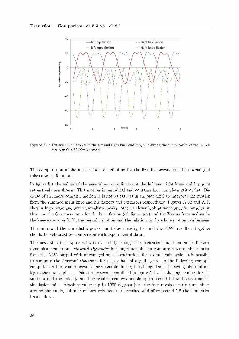
Extension � Comparison v1.5.5 vs. v1.8.1
‐80
‐60
‐40
‐20
0
20
40
0 1 2 3 4 5
hip/kn
ee flexion/extension [°]
time [s]
left hip flexion right hip flexion
left knee flexion right knee flexion
Figure 5.1: Extension and �exion of the left and right knee and hip joint during the computation of the muscle
forces with CMC for 5 seconds
The computation of the muscle force distribution for the �rst �ve seconds of the normal gait
takes about 15 hours.
In �gure 5.1 the values of the generalised coordinates at the left and right knee and hip joint
respectively are shown. This motion is periodical and contains four complete gait cycles. Be-
cause of the more complex motion it is not as easy as in chapter 4.2.2 to interpret the motion
from the summed main knee and hip �exors and extensors respectively. Figures A.32 and A.33
show a high noise and some unrealistic peaks. With a closer look at some speci�c muscles, in
this case the Gastrocnemius for the knee �exion (cf. �gure 5.2) and the Vastus Intermedius for
the knee extension (5.3), the periodic motion and the relation to the whole motion can be seen.
The noise and the unrealistic peaks has to be investigated and the CMC results altogether
should be validated by comparison with experimental data.
The next step in chapter 4.2.2 is to slightly change the excitation and then run a forward
dynamics simulation. Forward Dynamics is though not able to compute a reasonable motion
from the CMC output with unchanged muscle excitations for a whole gait cycle. It is possible
to compute the Forward Dynamics for nearly half of a gait cycle. In the following example
computation the results become unreasonable during the change from the swing phase of one
leg to the stance phase. This can be seen exempli�ed in �gure 5.4 with the angle values for the
subtalar and the ankle joint. The results seem reasonable up to second 1.1 and after that the
simulation fails. Absolute values up to 1000 degrees (i.e. the foot revolts nearly three times
around the ankle, subtalar respectively, axis) are reached and after second 1.5 the simulation
breaks down.
36

Extension � Comparison v1.5.5 vs. v1.8.1
0
0,25
0,5
0,75
1
0 1 2 3 4 5
norm
alised
excitation
time [s]
left
right
Figure 5.2: CMC calculated excitation of the Gastrocnemius
0
0,1
0,2
0,3
0 1 2 3 4 5
norm
alised
excitation
time [s]
left
right
Figure 5.3: CMC calculated excitation of the Vastus Intermedius
37

Extension � Comparison v1.5.5 vs. v1.8.1
0
45
90
0,7 0,8 0,9 1 1,1 1,2 1,3 1,4 1,5
exion / extension [°]
left ankle left subtalar
‐90
‐45
fle
time [s]
Figure 5.4: Angle values for subtalar and ankle joint of the left leg during a Forward Dynamics computation
after changing the excitation as described in chapter 4.2.2
Within this test case there was no way to produce reasonable and stable Forward Dynamics
results for longer time periods than in chapter 4.2.2. Under this conditions another change of
the excitation patterns is not expedient.
After second 1.7 no stable run of Forward Dynamics was possible. All this shows that there is
either a problem with the Forward Dynamics or the CMC results are not correct.
5.5.2 Scale Motions
In chapter 4.2.3 the angle of the degree of freedom of the hip �exion/extension is scaled by �ve
percent. In this test case the same scaling is done for a longer period of time (cf. �gure 5.5).
In �gures 5.6 and 5.7 the computed muscle excitations before and after the motion scaling are
compared.
The results seem reasonable and are very similar to those in chapter 4.2.3. The scaled excitations
seem a little bit smoothed compared against the unchanged excitations, this can especially be
seen in the �gure for the excitations of the Gluteus Maximus.
The results for excitations which should not a�ected by the scaling seem as reasonable as in
chapter 4.2.3, cf. �gures A.35.
The excitation of the right Quadriceps Femoris has not changed, as expected, but the excitation
of the left Quadriceps Femoris has changed slightly after the scaling (cf. �gure A.34). This is
not a result as expected because the change of the motion is for the left side and the right side
equal. This can not be explained easily. It has to be evaluated if this computation is possibly
38

Extension � Comparison v1.5.5 vs. v1.8.1
‐30
‐20
‐10
0
10
20
30
0 1 2 3 4 5
extension ‐h
ip [°] ‐
flexion
time [s]
original right changed right original left changed left
Figure 5.5: Flexion/Extension of the right hip joint; original and scaled as described in chapters 4.2.3 and 5.5.2
0
0,2
0,4
0,6
0 1 2 3 4 5
norm
alised
excitation
time [s]
original right scaled right original left scaled left
Figure 5.6: Comparison of CMC calculated excitation of right Gluteus Maximus for a longer period of time
before and after scaling the motion, �gure 5.5, and described in chapters 4.2.3 and 5.5.2
39

Extension � Comparison v1.5.5 vs. v1.8.1
0
0,5
1
1,5
2
0 1 2 3 4 5
norm
alised
excitation
time [s]
original right scaled right original left scaled left
Figure 5.7: Comparison of CMC calculated excitation of right Psoas and Iliacus for a longer period of time
before and after scaling the motion, �gure 5.5, and described in chapters 4.2.3 and 5.5.2
wrong and if other results are a�ected.
5.5.3 Create New Motions
Creating new motions is still a point of interest. The investigation of the kick motion is satis-
factory done in chapter 4.2.4, so that test case is not repeated and instead a new test case is
introduced in chapter 5.6.
At the Department of Mechanics at the KTH, Stockholm, there is currently a project to in-
vestigate jump motions and muscle force distributions during jumps with a performance based
algorithm. Therefore this test case is chosen instead to the previous kick motion.
5.6 Movements Without Ground Reactions
This test case is made to test the stability and accuracy of CMC for movements without ground
contact, like jumps. This is a special case, because OpenSim does not use contact conditions
between the subject and the ground. OpenSim uses residual forces normally applied to the
pelvis. If there are no ground reactions, there are also no residual forces and RRA cannot be
applied.
The test case is the normal gait example (2354) without the ground reaction forces. This motion
is then similar to walking through the air, like the leg movements of an athlete doing a long
jump.
40

Extension � Comparison v1.5.5 vs. v1.8.1
The �rst step is to run the Inverse Dynamics without ground reaction forces to get the correct
forces and torques at the generalised coordinates. The next step normally is the RRA but
because of the lack of ground reactions there are no residual forces applied to the pelvis and
therefore there is no need to run it. Now CMC computes the muscle forces.
The fast target always fails so that the slow target option has to be used. The run with the
slow target option �nishes and produces results. It seems that the subject is falling. It moves
freely and not along the prescribed coordinates recorded in the motion lab and computed with
Inverse Kinematics. Also the other degrees of freedom are not even similar to their prescribed
values. In �gure A.36 are the y coordinate of the pelvis and the progress of the values for the
right hip �exion and the lumbar extension shown exempli�ed. The original motion data (before
running CMC) can be seen in �gure A.37. It is obvious that these results are not similar to the
reality. The main question here is: Why does CMC compute a new motion, where it actually
should compute muscle force distributions?
5.7 Project Proposal � CMC and NMT, Two Muscle Force
Computation Approaches
The CMC algorithm of OpenSim is a new and progressive algorithm to compute muscle force
distributions. It has his strengths and weaknesses. A good opportunity to really test its limits
is to compare it to an other algorithm. The suggestion here is the NMT algorithm, because it
seems to �t in the gaps that CMC leaves.
5.7.1 Introduction
OpenSim is a freely available software package which o�ers the possibilities to build, exchange
and analyse computer models of the musculoskeletal system and run dynamic simulations of
movements.[4] Especially it o�ers a module to compute muscle forces and excitations for given
motions. This module is called CMC (Computing Muscle Control).
In general there are two ways of analysing muscle driven motions. On the one hand there are
tracking approaches and on the other hand there are performance-based dynamic optimisation
codes. Tracking algorithms determine muscle excitations that closely replicate an observed
movement. In contrast to this, performance-based dynamic optimisation is capable of generat-
ing novel movement based on a quanti�able objective (e.g. minimisation of metabolic energy
during gait). CMC falls in the category of tracking approaches.[25] A recent example for a fast
performance-based algorithm is the NMT (neuromusculoskeletal tracking) method.[22]
In this project it should be demonstrated that the use of simulations can improve treatment
outcomes for individuals with movement disorders. For that purpose the NMT method should
be integrated into OpenSim and compared to the CMC module.
Several case studies should be made to determine if general principles for treatment planning
can be elucidated from the insights gained from analysing simulations. Studies that retrospec-
41

Extension � Comparison v1.5.5 vs. v1.8.1
tively compare predictions from subject-speci�c simulations to the subject's actual outcomes
should also be made to evaluate whether the existing musculoskeletal models are su�ciently
accurate, and to establish the conditions under which the results of simulations are applicable
and which method (NMT, CMC) should be best used or if a combination of both is necessary
and possible.[4]
5.7.2 Methods that Could Be Used
The determination of �nding general principles for treatment planning requires many case stud-
ies. In this project three di�erent cases should be examined and compared. The case study used
for the validation for CMC[26], pedalling (ground contact during the whole simulation), should
be tested with NMT, the case study coming from the validation for NMT[22], height-jump (long
time without ground contact), should be tested with CMC even if RRA (Residual Reducing
Algorithm) cannot be applied, and a third case, healthy gait (ground reaction forces changing
strongly over the simulated cycle) should be applied to both algorithms.
5.7.3 Signi�cance of this Study
Even in a time where the computing power increases rapidly and more and faster supercomputers
become available the e�ciency of algorithms is still very important for highly complex models in
human movement simulations. This study should compare two of the most recent muscle force
computation approaches integrated in an open-source software package and make suggestions
for what cases and under which conditions they should be applied best. It should result in a fast,
e�cient, accurate and stable way to compute muscle forces even in very complex musculoskeletal
models. It also should be applicable to all kind of motions (with and without ground reaction
conditions).
42

6 Experiences and Future Work
In this chapter the author's opinion about the testing and the whole project is described.
6.1 Version 1.5.5
This chapter contains conclusions referring to chapter 4 and the OpenSim version 1.5.5.
All three di�erent test cases could be handled by OpenSim. The stability was di�erent and
therefore the way to work with OpenSim, too. Nevertheless, the results seemed to be reasonable
all the times and applicable to real cases as far as this can be evaluated without the comparison
to experiments.
Working in a motion lab requires good anatomical and technical knowledge. If the experimental
data is not collected precisely, the following simulation and simulation results are not feasible.
The testing experiences show that changing excitation patterns (cf. chapter 4.2.2) is not a
generally applicable procedure to create more complex movements. The user has to be very
experienced in anatomy and human movements to change the right muscle excitations; otherwise
the computed movement will not be realistic or predictable at all. Due to the complexity and
instability of human movement, just very small changes are possible. Manipulating excitation
patterns can be useful to slightly vary known motions or check in which direction a forward
simulation will lead, after a tendon transfer or other surgeries.
Scaling motions (cf. chapter 4.2.3) or producing a wholly new motion (cf. chapter 4.2.4) and
after that computing the needed muscle forces is an applicable way to analyse motions. The
problem is to obtain the reasonable ground reaction forces, which are needed for CMC to run.
It is thus not possible to use this analysis method to produce reasonable results without great
experience or preceding testing.
The choice of multi-body mechanics to analyse and simulate the human gait is very often
used and in most cases suitable. Developing an open source software (like OpenSim) is a very
ambitious and great project which can only succeed, if the software is accepted and used by the
scienti�c community. It is necessary for the developers that the user community reports bugs,
problems with actual modules and makes suggestions for useful new tools or modules. It seems
that the OpenSim developers try to reach these goals in di�erent ways. At Stanford (where the
main developer team works) beta versions and release candidates are tested extensively. The
OpenSim users' forum includes a feedback and bug-report section on the SimTK homepage,
which is the easiest way to communicate with OpenSim users worldwide. The quality of such
bulletin boards depends highly on the community itself and not only on the moderators. In the
43

Experiences and Future Work
users' forum, some questions are answered within two days and some never. Because the user
does not have the advantage of a real support team (like in the commercial software package
SIMM) he can try to get help from the community, but should never rely on it and always be
prepared for �nding a solution to the problem on his own.
On 21 August 2008 an OpenSim User's Guide was published, [7]. In this manual, the basic
functions of OpenSim and its underlying mathematics are described. The most of the docu-
mentation is very useful and understandable. In chapter 16 of the User's Guide the RRA is
described (chapter 17 for CMC respectively). As mentioned in chapter 3.3.1 the documentation
is not su�cient to understand the basic principles of those modules. The reference quoted have
to be consulted.
The modules IK and ID are working stably and produce comprehensible results. The documen-
tation is su�ciently described in detail in the User's Guide. Those modules are necessary basic
features for a biomechanical simulation software. OpenSim has a stable basis.
The modules RRA and CMC are working very unstably, as described in chapter 4.4. The crash
report �les contain no relevant information, so that the user can not �x the problem on his own
and has to wait for an o�cial statement or update. This is a major problem, because these two
modules are unique features of OpenSim and should distinguish this software from others like
SIMM. OpenSim cannot provide this if it does not work stably enough.
It is suggested to run the RRA module more than one time. Normally, more than two passes
are not necessary. The adjusting values after the second pass should be very small. If they are
not small enough, there is perhaps a problem existing in the model or with the ground reaction
forces.
OpenSim o�ers the possibility to do Forward Dynamics. This is absolutely correct from a
numerical and mathematical point of view. However, a lot of experimental data to compute
the muscle excitation is needed and prior Inverse Kinematics and Inverse Dynamics have to
be done, so that for most of the users and application areas it is not a real forward simulation
but could be called a semi-forward simulation. The documentation and the o�cial statement to
the instability of Forward Dynamics (cf. chapter 4.4) is inconsistent with the test experiences.
This leads to a major problem. Forward Dynamics is a necessary module for biomechanical
simulation software. If the user can not use it and the user's guide does not give suitable
explanations, the user can not count on that feature and is forced to use another software with
greater reliability.
The most important feature is, due to the fact that OpenSim is not designed for creating or
making major model changes, the import function. Because the SIMM import module does not
yet work for most of the SIMM models, the software is very limited in its range of application.
This problem was recognised by the development team and will hopefully lead to a practicable
solution soon.
The idea and intention of OpenSim is great. In the version 1.5.5 the basic functions are working
�ne. Some major problems are recognised and the developers are working them up. The
documentation is a minor problem and it is to be expected that it will become better, with
more users working with it and the longer stable versions of all modules are available.
44

Experiences and Future Work
Working with OpenSim is not recommendable at the moment to users expecting great reliability.
It is a good alternative for experimental usage and showing some examples of biomechanical
engineering in teaching.
6.2 Version 1.8.1
This chapter contains conclusions referring to chapter 5 and the OpenSim version 1.8.1.
Unfortunately there is still only a Windows 32-Bit version available. There is no support for
other OS like Linux or MacOS and also no support for any 64-Bit systems. I think that should
be one of the next steps, but it is not totally up to the development team of OpenSim but rather
of the SimTK-group, which is responsible for the numerical background and the multi-body core
engine.
In the test cases all SIMM models could be imported. This leads to a greater variety of possible
applications of OpenSim even in running projects which are based on SIMM models. It does not
lead to better results of OpenSim or to extension of what OpenSim is able to do. The SIMM
compatibility is a very basic feature and absolutely necessary for OpenSim to compete in the
market for biomechanical simulation software tools.
The User's Guides and the support in an open source project are always one of the biggest prob-
lems. From version 1.5.5 to v1.8.1 there is no big improvement of the User's Guides especially
the chapter about the unique features RRA and CMC is still not su�cient and additional
papers has to be consulted to understand these mechanisms. In the OpenSim project wiki there
is an additional information document to RRA and CMC .[18] As written in chapter 5.4.1 it is
not possible for the user to fully understand how RRA works, because of a discrepancy between
the User's Guide and the GUI. Although it is possible to use features which are working but
without feasible explanations, it is often not satisfying and it is even more a problem if the user
wants to change details or works with non standard cases, so it has to be checked if the speci�c
algorithm can be used and in what way it computes its results.
In most of the cases in which OpenSim cannot �nd a solution or has a problem it does not
completely break down anymore but instead it produces an error message with an error number.
The messages are normally very short so that it is sometimes hard for the user to �nd out what
exactly went wrong. The error numbers are not helpful because there is no explanation for
them. The documentation of those error numbers has to be published.
Another documentation problem is that there are some options which are not available but
hidden in the XML control �les and can only be activated by editing those control �les. It is
confusing if the User's Guide does not mention them or, even worse, if it describes them in a
wrong way. The problem exists the other way round, too: in the XML �les are some options
which do not have any e�ect on the computation or the output.
The stability of CMC has increased signi�cantly. With now longer test cases and more stable
simulations possible this module has become more interesting. Some results of the test cases
seem reasonable and some simply do not. There is no real advance if the simulations are more
45

Experiences and Future Work
stable but do not provide good results, so that the results have to be validated and compared
with measurements in more than one case study.
The main idea of inventing CMC (and not using an old muscle force computation algorithm) was
to make muscle force computation faster and possible for users even with lower level computing
resources. The slow target option seem to be really slow, so that possibly that scope is not
reached. A performance study would be interesting and should provide additional insight into
stability and computing speed.
The new test case shows that the new stability of CMC is fading away for motions without
ground reaction forces. There is no o�cial statement that CMC is not suitable for such motions
and there are so far no other user reports in the users' forum which include positive statement
about such motions. The main question wich is left here is: Is it possible to run CMC for
motions without ground reactions?
All theses results about CMC mainly lead to the project proposal in chapter 5.7.
The instability of Forward Dynamics, as described in chapter 4.4, is still a problem and no
further o�cial announcements has been made. Due to this fact and the complexity of the
musculoskeletal problems, OpenSim and the Forward Dynamics function should only be used in
the way suggested in the User's Guide: The �rst step is to track a motion and do the calculation
steps including the computation of the muscle forces and excitations with CMC, the second step
is to vary slightly the muscle excitations to do in a third step a forward dynamic simulation.
My general conclusion for the comparison between version 1.5.5 and 1.8.1 is that some modules
has become considerably more stable, but slow and maybe the results are not always as good
as with the older version.
This shows that OpenSim is still in an early stage of development. The announced improvement
of the forward dynamics module gives reason for hope. OpenSim has a stable basis and a great
potential, the newest version is one big step in the right direction.
46

Bibliography
[1] Å. Björck: Numerical methods for least squares problems. Society for Industrial and
Applied Mathematics, Philadelphia, 1996.
[2] C. Lawrence, J.L. Zhou and A.L. Tits: User's Guide for CFSQP Version 2.5: A C
Code for Solving (Large Scale) Constrained Nonlinear (Minimax) Optimization Problems,
Generating Iterates Satisfying All Inequality Constraints, Electrical Engineering Depart-
ment and Institute for Systems Research at the University of Maryland, College Park MD
20742, April 1997.
[3] S. Delp: Surgery simulation: A computer graphics system to analyze and design mus-
culoskeletal reconstructions of the lower limb. Stanford University, Palo Alto, California,
1990.
[4] S.L. Delp, F.C. Anderson, A.S. Arnold, P. Loan, A. Habib, C.T. John,E.Guendelman and D.G. Thelen: OpenSim: Open-source Software to Create and An-
alyze Dynamic Simulations of Movement. IEEE Transactions on Biomedical Engineering,
Vol. 54, No. 11, p. 1940�1950, November 2007.
[5] S.L. Delp and J.P. Loan: A Graphics-Based Software System to Develop and Analyze
Models of Musculoskeletal Structures. Computers in Biology and Medicine, Vol. 25, No. 1,
p. 21�34, 1995.
[6] S.L. Delp and J.P. Loan: A Computational Framework for Simulating and Analyzing
Human and Animalmovement. IEEE Computing in Science & Engineering, Vol. 2, No. 5,
p. 46�55, September/October 2000.
[7] S. Delp et al.: OpenSim User's Guide 1.01, Stanford University, California, USA,
https://simtk.org/home/opensim, August 2008.
[8] E. Hairer, C. Lubich and M. Roche: The Numerical Solution of Di�erential-Algebraic
Systems by Runge-Kutta Methods. Springer Verlag, Berlin/Heidelberg/New York, 1989.
[9] E. Hairer, S.P. Nørsett and G. Wanner: Solving Ordinary Di�erential Equations I,Nonsti� Problems. Springer Verlag, Berlin/Heidelberg/New York, 1987.
[10] S. Heintz and E.M. Gutierrez-Farewik: Static optimization of muscle forces during
gait in comparison to EMG-to-force processing approach. Gait & posture, Vol. 26, No. 2,
p. 279�288, 2007.
[11] M.G. Hollars, D.E. Rosentahl and M.A. Sherman: SD/FAST User's Manual B.2,
Symbolic Dynamics, Inc., Mountain View, CA, USA, September 1994.
[12] P. Loan, S. Delp, K. Smith and K. Blaikie: Dynamics Pipeline User Guide 1.2,
47

Bibliography
MusculoGraphics, Inc., Santa Rosa, CA, USA, June 2004.
[13] P. Loan, D. Wyles and S. Delp: Dynamics Pipeline User Guide 1.2, MusculoGraphics,
Inc., Evanston, IL, USA, January 2000.
[14] C.-D. Munz and T. Westermann: Numerische Behandlung gewöhnlicher und partiellerDi�ernzialgleichungen. Springer Verlag, Berlin/Heidelberg/New York, 2006.
[15] OpenSim Project Wiki: Guidelines for using, http://wiki.simtk.org/opensim/rraCmcPage,
accessed: May 22nd, 2009.
[16] OpenSim Project Wiki: Optimizers, http://wiki.simtk.org/opensim/Optimizers, ac-
cessed: May 13th, 2009.
[17] OpenSim Project Wiki: Optimizers Round Up, http://wiki.simtk.org/opensim/ Op-
timizers?action=AttachFile&do=get&target=optimizer_roundup.txt, accessed: May 6th,
2009.
[18] OpenSim Project Wiki: Theory of RRA and CMC, http://wiki.simtk.org/opensim/
FrontPage?action=AttachFile&do=get&target=theoryCMC.doc, accessed: April 22nd,
2009.
[19] OpenSim Users Forum: Ayman Habib, https://simtk.org/ forum/mes-
sage.php?msg_id=2063, accessed: May 13th, 2009.
[20] C.C. Raasch, F.E. Zajac, B. Ma and W.S. Levine: Muscle coordination of maximum-
speed pedaling. Journal of Biomechanics, Vol. 30, No. 6, p. 595�602, 1997.
[21] L.M. Schutte, M.M. Rodgers, F.E. Zajac and R.M. Glaser: Improving the e�-
cacy of electrical stimulation-induced leg cycle ergometry: an analysis based on a dynamic
musculoskeletalmodel. IEEE Transaction on Rehabilitation Engineering, Vol. 1, No. 2,
p. 109�125, 1993.
[22] A. Seth and M.G. Pandy: A neuromusculoskeletal tracking method for estimating in-
dividual muscle forces in human movement. Journal of Biomechanics, Vol. 40, No. 2,
p. 356�366, 2007.
[23] M. Sherman: SimBody User's Manual early access release 0.7,
http://simtk.org/home/simbody, August 2007.
[24] SIMM: Software for Interactive Musculoskeletal Modeling,
http://www.musculographics.com, MusculoGraphics, Inc. 2008.
[25] D.G. Thelen and F.C. Anderson: Using computed muscle control to generate forward
dynamic simulations of human walking from experimental data. Journal of Biomechanics,
Vol. 39, No. 6, p. 1107�1115, 2006.
[26] D.G. Thelen, F.C. Anderson and S.L. Delp: Generating dynamic simulations of
movement using computed muscle control. Journal of Biomechanics, Vol. 36, No. 3, p. 321�
328, 2003.
[27] J. Wagner and H.P. Mlejnek: Dynamik 1 Vorlesungsunterlagen. Institut für Statik
und Dynamik der Luft- und Raumfahrtkonstuktionen, Universität Stuttgart, Germany,
48

Bibliography
2008.
[28] M. Wei: Supremum and stability of weighted pseudoinverses and weighted least squares
problems. Nova Science, New York, 2001.
[29] Wikipedia: Non-linear least squares, http://en.wikipedia.org/wiki/Non-
linear_least_squares, accessed: November 11th, 2008.
[30] Wikipedia: IPOPT, http://en.wikipedia.org/wiki/IPOPT, accessed: April 17th, 2009.
[31] D.A. Winter: Biomechanics and Motor Control of Human Movement. John Wiley and
Sons, Inc., Waterloo, Ontario, Canada, 3. Edition, 2005.
[32] F.E. Zajac: Muscle and tendon: properties, models, scaling and application to biomechan-
ics and motor control. CRC Critical Reviews in Biomedical Engineering, Vol. 17, No. 4,
p. 359�411, 1989.
49


A Appendix
This appendix contains additional �gures resulting of the test cases discussed in chapter 4 and
5 and source codes that were used to handle and modify motion data �les.
51

Appendix
A.1 Motion Laboratory
Table A.1: Description of the marker positions for the motion lab experiments
Marker Position
PL1 Pelvis Left ASIS
PR1 Pelvis Right ASIS
PR2 Pelvis Right PSIS
RF1 Right Greater Trochanter
RF2 Right Medial Femural Condyle
RF3 Right Lateral Femural Condyle
RT1 Right Medial Tibia
RT2 Right Lateral Tibia/Fibular Head
RT3 Right Medial Malleolus
RT4 Right Lateral Malleolus
PL1PR1
RF3 RF2
RT1RT2
PR2
RT3RT4
PR1
RF3
RT2
Figure A.1: Marker positions for the motion lab recordings
52

Appendix
A.1.1 Hip Flexion/Extension
0 50 100 150 200 250 300 350 400 450−20
−15
−10
−5
0
5
10
15
20
timesteps
exte
rnal
− R
otat
ion
[°] −
inte
rnal
Figure A.2: Hip Flexion/Extension - Hip transverse
plane
0 50 100 150 200 250 300 350 400 450−30
−25
−20
−15
−10
−5
0
5
10
15
20
25
timesteps
exte
rnal
− R
otat
ion
[°] −
inte
rnal
Figure A.3: Hip Flexion/Extension - Knee transverse
plane
0 50 100 150 200 250 300 350 400 450−30
−20
−10
0
10
20
30
40
50
60
70
timesteps
Ext
ensi
on −
[°] −
Fle
xion
Figure A.4: Hip Flexion/Extension - Hip sagittal plane
0 50 100 150 200 250 300 350 400 450−20
−10
0
10
20
30
40
50
60
70
80
90
timesteps
Ext
ensi
on −
[°] −
Fle
xion
Figure A.5: Hip Flexion/Extension - Knee sagittal
plane
0 50 100 150 200 250 300 350 400 450−40
−30
−20
−10
0
10
20
timesteps
Abd
uctio
n −
[°] −
Add
uctio
n
Figure A.6: Hip Flexion/Extension - Hip frontal plane
0 50 100 150 200 250 300 350 400 450
−20
−10
0
10
20
30
40
timesteps
Val
gus
− [°
] − V
arus
Figure A.7: Hip Flexion/Extension - Knee frontal
plane
53

Appendix
A.1.2 Hip Ab-/Adduction
20 40 60 80 100 120 140 160 180 200 2200
5
10
15
20
25
30
35
40
timesteps
exte
rnal
− R
otat
ion
[°] −
inte
rnal
Figure A.8: Hip Ab-/Adduction - Hip transverse plane
20 40 60 80 100 120 140 160 180 200 220−30
−25
−20
−15
−10
−5
0
5
10
15
20
25
timesteps
exte
rnal
− R
otat
ion
[°] −
inte
rnal
Figure A.9: Hip Ab-/Adduction - Knee transverse
plane
20 40 60 80 100 120 140 160 180 200 220−30
−20
−10
0
10
20
30
40
50
60
70
timesteps
Ext
ensi
on −
[°] −
Fle
xion
Figure A.10: Hip Ab-/Adduction - Hip sagittal plane
20 40 60 80 100 120 140 160 180 200 220−40
−30
−20
−10
0
10
20
30
40
50
60
70
timesteps
Ext
ensi
on −
[°] −
Fle
xion
Figure A.11: Hip Ab-/Adduction - Knee sagittal plane
20 40 60 80 100 120 140 160 180 200 220−90
−80
−70
−60
−50
−40
−30
−20
−10
0
timesteps
Abd
uctio
n −
[°] −
Add
uctio
n
Figure A.12: Hip Ab-/Adduction - Hip frontal plane
20 40 60 80 100 120 140 160 180 200 220
−20
−10
0
10
20
30
40
timesteps
Val
gus
− [°
] − V
arus
Figure A.13: Hip Ab-/Adduction - Knee frontal plane
54

Appendix
A.1.3 Hip Rotation
240 260 280 300 320 340 360 380 40025
30
35
40
45
50
55
60
65
70
timesteps
exte
rnal
− R
otat
ion
[°] −
inte
rnal
Figure A.14: Hip Rotation - Hip transverse plane
240 260 280 300 320 340 360 380 400−30
−25
−20
−15
−10
−5
0
5
10
15
20
25
timesteps
exte
rnal
− R
otat
ion
[°] −
inte
rnal
Figure A.15: Hip Rotation - Knee transverse plane
240 260 280 300 320 340 360 380 400−30
−20
−10
0
10
20
30
40
50
60
70
timesteps
Ext
ensi
on −
[°] −
Fle
xion
Figure A.16: Hip Rotation - Hip sagittal plane
240 260 280 300 320 340 360 380 400−20
−10
0
10
20
30
40
50
60
70
80
90
timesteps
Ext
ensi
on −
[°] −
Fle
xion
Figure A.17: Hip Rotation - Knee sagittal plane
240 260 280 300 320 340 360 380 400−40
−30
−20
−10
0
10
20
timesteps
Abd
uctio
n −
[°] −
Add
uctio
n
Figure A.18: Hip Rotation - Hip frontal plane
240 260 280 300 320 340 360 380 400
−20
−10
0
10
20
30
40
timesteps
Val
gus
− [°
] − V
arus
Figure A.19: Hip Rotation - Knee frontal plane
55

Appendix
A.1.4 Knee Flexion/Extension
20 40 60 80 100 120 140−20
−15
−10
−5
0
5
10
15
20
timesteps
exte
rnal
− R
otat
ion
[°] −
inte
rnal
Figure A.20: Knee Flexion/Extension - Hip transverse
plane
20 40 60 80 100 120 140
−20
−10
0
10
20
30
40
timesteps
exte
rnal
− R
otat
ion
[°] −
inte
rnal
Figure A.21: Knee Flexion/Extension - Knee trans-
verse plane
20 40 60 80 100 120 140−30
−20
−10
0
10
20
30
40
50
60
70
timesteps
Ext
ensi
on −
[°] −
Fle
xion
Figure A.22: Knee Flexion/Extension - Hip sagittal
plane
20 40 60 80 100 120 140−20
−10
0
10
20
30
40
50
60
70
80
90
timesteps
Ext
ensi
on −
[°] −
Fle
xion
Figure A.23: Knee Flexion/Extension - Knee sagittal
plane
20 40 60 80 100 120 140−40
−30
−20
−10
0
10
20
timesteps
Abd
uctio
n −
[°] −
Add
uctio
n
Figure A.24: Knee Flexion/Extension - Hip frontal
plane
20 40 60 80 100 120 140
−20
−10
0
10
20
30
40
timesteps
Val
gus
− [°
] − V
arus
Figure A.25: Knee Flexion/Extension - Knee frontal
plane
56

Appendix
A.2.2 Change Excitation Patterns
0,3
0,4
0,5
d excitation
original changed
0
0,1
0,2
0 0,2 0,4 0,6 0,8 1
norm
alised
normalised time
Figure A.26: Comparison of original and changed excitations of right hip extensors (Iliopsoas) for the test case
described in chapter 4.2.2
5
10
15
20
25
] ‐extension
original
excitation changed
‐25
‐20
‐15
‐10
‐5
0
0 0,2 0,4 0,6 0,8 1
flexion
‐kn
ee angle [°]
normalised time
Figure A.27: Right knee �exion/extension resulting from original and changed excitations shown in �gure A.26
and described in chapter 4.2.2
57

Appendix
A.2 Manipulate Motions
A.2.1 Musculoskeletal Geometry
Table A.2: Muscle-tendon Parameters for 43 Lower-Limb Muscles [3]
peak muscle optimal �bre pennation tendon slack tendon
force length angle length length/�bre
muscle(FM
0
) (lM0
)(α)
(lTS
)length
(N) (cm) (degrees) (cm)(lTS
)/
(lM0
)hip muscles
gluteus medius1 550 5.4 8 7.8 1.4
gluteus medius2 380 8.4 0 5.3 0.6
gluteus medius3 435 6.5 19 5.3 0.8
gluteus minimus1 180 6.8 10 1.6 0.2
gluteus minimus2 190 5.6 0 2.6 0.5
gluteus minimus3 215 3.8 1 5.1 1.3
gluteus maximus1 380 14.2 5 12.5 0.9
gluteus maximus2 550 14.7 0 12.7 0.9
gluteus maximus3 370 14.4 5 14.5 1.0
adductor magnus1 345 8.7 5 6.0 0.7
adductor magnus2 310 12.1 3 13.0 1.0
adductor magnus3 445 13.1 5 26.0 2.0
adductor longus 420 13.8 6 11.0 0.8
adductor brevis 285 13.3 0 2.0 0.2
pectineus 175 13.3 0 0.1 0.1
iliacus 430 10.0 7 9.0 0.9
psoas 370 10.4 8 13.0 1.3
quadratus femoris 255 5.4 0 2.4 0.4
pemelli 110 2.4 0 3.9 1.6
piriformis 295 2.6 10 11.5 4.4
hip and knee muscles
rectus femoris 780 8.4 5 34.6 4.0
semimembranosus 1030 8.0 15 35.9 4.5
semitendinosus 330 20.1 5 26.2 1.3
biceps femoris (lh) 720 10.9 0 34.1 3.1
gracilis 110 35.2 3 14.0 0.4
sartorius 105 57.9 0 4.0 0.1
tensor fasciae latae 155 9.5 3 42.5 4.5
knee muscles
vastus medialus 1295 8.9 5 12.6 1.4
vastus intermedius 1235 8.7 3 13.6 1.6
vastus lateralis 1870 8.4 5 15.7 1.9
biceps femoris (sh) 400 17.3 23 10.0 0.6
knee and ankle muscles
medial gastrocnemius 1115 4.5 17 40.8 9.0
lateral gastrocnemius 490 6.4 8 38.5 6.0
ankle muscles
soleus 2830 3.0 25 26.8 8.9
tibialis posterior 1270 3.1 12 31.0 10.0
�. digitorum longus 310 3.4 7 40.0 11.8
�. hallucis longus 320 4.3 10 38.0 8.8
peroneus brevis 350 5.0 5 16.1 3.2
pernoeus longus 755 4.9 10 34.5 7.0
tibialis anterior 600 9.8 5 22.3 2.2
pernoeus tertius 90 7.9 13 10.0 1.3
ext. digitorum longus 340 10.2 8 34.5 3.4
ext. hallucis longus 110 11.1 6 30.5 2.6
58

Appendix
A.2.3 Scale Motions
0,25
0,3
0,35
0,4
d excitation
original
scaled
0
0,05
0,1
0,15
0,2
0 0,2 0,4 0,6 0,8 1
norm
alised
normalised time
Figure A.28: Comparison of CMC calculated excitation of right Quadriceps Femoris before and after scaling
the motion, �gure 4.7, and described in chapter 4.2.3
0,8
1
1,2
d excitation
original scaled
0
0,2
0,4
0,6
0 0,2 0,4 0,6 0,8 1
norm
alised
normalised time
Figure A.29: Comparison of CMC calculated excitation of right Planta�exors before and after scaling the
motion, �gure 4.7, and described in chapter 4.2.3
59

Appendix
A.2.4 Create New Motions
0,8
1
1,2
muscle force
hip extensor hip flexor
knee flexor knee extensor
0
0,2
0,4
0,6
0 0,2 0,4 0,6 0,8 1
norm
alised
m
normalised time
Figure A.30: Separate muscle forces of the main �exors/extensors of the hip/knee during knee bending de-
scribed in chapter 4.2.4, the separate muscle forces are shown in �gure 4.12
0,8
1
1,2
muscle force
hip extensor hip flexor
knee flexor knee extensor
0
0,2
0,4
0,6
0 0,2 0,4 0,6 0,8 1
norm
alised
m
normalised time
Figure A.31: Separate muscle forces of the main �exors/extensors of the hip/knee during the kick movement
described in chapter 4.2.4, the summed muscle forces are shown in �gure 4.13
60

Appendix
A.3 Extension
A.3.1 Change Excitation Patterns
0
0,5
1
1,5
2
2,5
3
0 1 2 3 4 5
norm
alised
exten
sion
time [s]
left right
Figure A.32: Summation of the CMC calculated excitations of the main knee �exors
0
0,1
0,2
0,3
0 1 2 3 4 5
norm
alised
excitation
time [s]
left right
Figure A.33: Summation of the CMC calculated excitations of the main knee extensors
61

Appendix
A.3.2 Scale Motions
0
0,1
0,2
0,3
0 1 2 3 4 5
norm
alised
excitation
time [s]
original left scaled left original right scaled right
Figure A.34: Comparison of CMC calculated excitation of right Quadriceps Femoris for a longer period of time
before and after scaling the motion, �gure 5.5, and described in chapters 4.2.3 and 5.5.2
0
0,25
0,5
0,75
1
1,25
0 1 2 3 4 5
norm
alised
excitation
time [s]
original left scaled left original right scaled right
Figure A.35: Comparison of CMC calculated excitation of right Planta�exors for a longer period of time before
and after scaling the motion, �gure 5.5, and described in chapters 4.2.3 and 5.5.2
62

Appendix
A.3.3 Movements Without Ground Reactions
‐120
‐80
‐40
0
‐80
‐60
‐40
‐20
0
20
40
60
0 1 2 3 4 5
absolute y coo
rdinate [m
]
flexion
/exten
sion
[°]
time [s]
hip flexion right lumbar extension pelvis y
Figure A.36: CMC computed motion without ground reaction forces: y coordinate of the pelvis, angles of the
right hip �exion and the lumbar extension
0
0,1
0,2
0,3
0,4
0,5
0,6
0,7
0,8
0,9
1
‐50
‐40
‐30
‐20
‐10
0
10
20
30
40
50
0 1 2 3 4 5
absolute y coo
rdinate [m
]
Flexion/Extension [°]
time [s]
hip flexion right lumbar extension pelvis y
Figure A.37: Inverse Dynamics computed motion without ground reaction forces: y coordinate of the pelvis,
angles of the right hip �exion and the lumbar extension
63

Appendix
A.4 Source Codes
A.4.1 Motion Laboratory
Listing A.1: MATLAB source code for calculating joint angles (of hip �exion/extension)
1 imp o r t f i l e HipFlexionExtens ion . txt ;
2
3 %a l l o c a t i n g matr i ce s
4 PHI_p = ze ro s ( l ength ( data ) ,3 ) ;
5 PHI_h = ze ro s ( l ength ( data ) ,3 ) ;
6 PHI_k = ze ro s ( l ength ( data ) ,3 ) ;
7 KJC = ze ro s ( l ength ( data ) ,3 ) ; %knee j o i n t c en t r e
8 FC = ze ro s ( l ength ( data ) ,3 ) ; %"femur cent r e "
9 TC = ze ro s ( l ength ( data ) ,3 ) ; %"t i b i a c en t r e "
10 AJC = ze ro s ( l ength ( data ) ,3 ) ; %ankle j o i n t c en t r e
11 HJC = ze ro s ( l ength ( data ) ,3 ) ; %hip j o i n t c ent r e
12 PO = ze ro s ( l ength ( data ) ,3 ) ; %p e l v i s cos o r i g i n
13
14 PR1=ze ro s ( l ength ( data ) ,3 ) ;
15
16 f o r i = 1 : l ength ( data )
17 % de f i n i t i o n o f the p e l v i s cos
18 PR1 = [ data ( i , 1 8 ) data ( i , 1 9 ) data ( i , 2 0 ) ] ' ;
19 PR1_all ( i , 1 : 3 )=PR1 ;
20 PL1 = [ data ( i , 2 4 ) data ( i , 2 5 ) data ( i , 2 6 ) ] ' ;
21 ey_p = (PR1 −PL1) /norm(PR1 −PL1) ;22 PR2 = [ data ( i , 2 1 ) data ( i , 2 2 ) data ( i , 2 3 ) ] ' ;
23 lambda = ( (PR2 −PR1) '∗ey_p) /(ey_p '∗ ey_p) ;24 ex_p = PR2 −PR1 − lambda ∗ ey_p ; %not normal i sed
25 ex_p = ex_p / norm(ex_p) ; %normal i sed
26 ez_p=c ro s s (ex_p , ey_p) ; %not normal i sed
27 ez_p=ez_p/norm(ez_p) ; %normal i sed
28 T_p = [ ex_p ey_p ez_p ] ;
29 %Transformationmatr ix world in to p e l v i s at t imestep i
30 EX_p( i , 1 : 3 )=ex_p ;
31 EY_p( i , 1 : 3 )=ey_p ;
32 EZ_p( i , 1 : 3 )=ez_p ;
33 %se t the o r i g i n o f the p e l v i s coo rd ina te system in the middle between
34 %PR1 and PL1
35 po= 0.5∗ (PR1 + PL1) ;
36 PO( i , 1 : 3 ) = po ' ;
37
38 %the hip j o i n t c en t r e i s assumed to be (−50 , 0 , −50) '39 %from PR1 in the p e l v i s coo rd ina te system
40 PR1_p=T_p∗PR1+po ;41 hjc_p=PR1_p + [−50 0 −50] ' ;
42 hjc = T_p\( hjc_p−po ) ;43 HJC( i , 1 : 3 ) = hjc ' ;
44
45 %ca l c u l a t e the ankle j o i n t c en t r e
46 RT3 = [ data ( i , 2 7 ) data ( i , 2 8 ) data ( i , 2 9 ) ] ' ;
47 RT4 = [ data ( i , 3 0 ) data ( i , 3 1 ) data ( i , 3 2 ) ] ' ;
64

Appendix
48 a j c = 0 .5∗ (RT4+RT3) ;
49 AJC( i , 1 : 3 )=ajc ' ;
50
51 %cacu l a t i ng a s s i s t a n c e po in t s fc , t c :
52 %ca l c u l a t i n g the cent r e o f RT1, RT2
53 RT1 = [ data ( i , 1 2 ) data ( i , 1 3 ) data ( i , 1 4 ) ] ' ;
54 RT2 = [ data ( i , 9 ) data ( i , 1 0 ) data ( i , 1 1 ) ] ' ;
55 tc = 0 .5∗ (RT2+RT1) ;
56 TC( i , 1 : 3 )=tc ' ;
57 %ca l c u l a t i n g the cent r e o f RF2 , RF3
58 RF2 = [ data ( i , 6 ) data ( i , 7 ) data ( i , 8 ) ] ' ;
59 RF3 = [ data ( i , 3 ) data ( i , 4 ) data ( i , 5 ) ] ' ;
60 f c = 0 .5∗ (RF3+RF2) ;
61 FC( i , 1 : 3 )=fc ' ;
62
63 %c a l c l u l a t e the knee j o i n t c ent r e under the assumption , that the
64 %in t e r s e c t i o n o f the vec to r from a j c to tc and the vec to r
65 %from hjc to f c d e f i n e s i t
66 temp1=[( h jc (1 )−f c (1 ) ) ( tc (1 )−a j c (1 ) ) ;
67 ( h jc (2 )−f c (2 ) ) ( tc (2 )−a j c (2 ) ) ] \ [ ( a j c (1 )−hjc (1 ) ) ( a j c (2 )−hjc (2 ) ) ] ' ;68 k j c= hjc+ temp1 (1) ∗( hjc−f c ) ;69 KJC( i , 1 : 3 )=kjc ' ;
70
71 %de f i n i t i o n o f the hip cos , o r i g i n i s k j c
72 %ez_h = ( k j c − hjc ) /norm( k j c − hjc ) ;
73 ez_h = ( f c − hjc ) /norm( f c − hjc ) ;
74 ey_h = (RF3−RF2) /norm(RF3−RF2) ;75 ex_h = c ro s s (ey_h , ez_h) ; %not normal i sed
76 ex_h = ex_h /norm(ex_h) ; % normal i sed
77 T_h = [ ex_h ey_h ez_h ] ;
78 %Transformationmatr ix world in to hip at t imestep i
79 T_ph= T_h/T_p;
80 %Transformationmatr ix p e l v i s i n to hip at t imestep i
81
82 EX_h( i , 1 : 3 )=ex_h ;
83 EY_h( i , 1 : 3 )=ey_h ;
84 EZ_h( i , 1 : 3 )=ez_h ;
85
86 %de f i n t i o n o f the knee cos , o r i g i n i s a j c
87 %ez_k = ( a j c − k j c ) /norm( a j c − k j c ) ;
88 ez_k = ( a j c − tc ) /norm( a j c − tc ) ;
89 ey_k = (RT4−RT3) /norm(RT4−RT3) ;90 ex_k = c ro s s (ey_k , ez_k ) ; %not normal i sed
91 ex_k = ex_k /norm(ex_k) ; % normal i sed
92 T_k = [ ex_k ey_k ez_k ] ;
93 %Transformationmatr ix world in to hip at t imestep i
94 T_hk= T_k/T_h;
95 %Transformationmatr ix hip in to knee at t imestep i
96
97 EX_k( i , 1 : 3 )=ex_k ;
98 EY_k( i , 1 : 3 )=ey_k ;
99 EZ_k( i , 1 : 3 )=ez_k ;
100
65

Appendix
101 %ca l c u l a t i n g the Euler ang l e s with convent ion zyx ( Tait−Bryan )102 %pe l v i s in r e sp e c t to world
103 %phi = transve r s e , s a g i t t a l , f r o n t a l
104
105 phi_p=[atan (T_p(1 , 2 ) /T_p(1 , 1 ) ) a s in (−T_p(1 , 3 ) ) atan (T_p(2 , 3 ) /T_p(3 , 3 ) ) ] ;
106 PHI_p( i , 1 : 3 )=phi_p∗180/ p i ;107
108 phi_h=[−atan (T_ph(1 , 2 ) /T_ph(1 , 1 ) ) a s in (−T_ph(1 , 3 ) ) atan (T_ph(2 , 3 ) /T_ph(3 , 3 ) ) ] ;
109 PHI_h( i , 1 : 3 )=phi_h∗180/ p i ;110
111 phi_k=[−atan (T_hk(1 , 2 ) /T_hk(1 , 1 ) ) −a s in (−T_hk(1 , 3 ) ) atan (T_hk(2 , 3 ) /T_hk(3 , 3 ) )
] ;
112 PHI_k( i , 1 : 3 )=phi_k∗180/ p i ;113 end
66

Appendix
A.4.2 Scale Motions
Listing A.2: Perl source code for modifying motion �les
1 # read ∗ .mot f i l e −−−−−−−−−−−−−−−−−−−−−−−−−−−−−−−−−−−−−2
3 $ f i l e = ' s o u r c e f i l e . s to ;
4 #READIN: p r i n t " F i l e : " ;
5 #$ f i l e = <STDIN> ;
6
7 i f ( open (MOTION, $ f i l e ) )
8 {
9 @l ines = <MOTION>;
10 c l o s e (MOTION) ;
11 }
12 e l s e
13 {
14 pr in t " Error , t ry again ! \n " ;
15 goto READIN;
16 }
17 # end read in−−−−−−−−−−−−−−−−−−−−−−−−−−−−−−−−−−−−−−−−−18
19 # clean f i l e and s o r t header out−−−−−−−−−−−−−−−−−−−−−−20 f o r each $each ( @l ines )
21 {
22
23 i f ( $each =~ /^(\ s ∗[−\d ] ) /)24 {
25 $each =~ s/^\ s+//;
26 $each =~ s /\n/\n eo l /g ;
27 $each =~ s / [\ s ]+/\n/g ;
28 @temp = s p l i t (/\n/ , $each ) ;
29 push (@numbers ,@temp) ;
30 }
31 e l s e
32 {
33 push (@header , $each ) ;
34 }
35 }
36 $ l a s t=@header ;
37 whi le ( $header [ $ l a s t −1] =~ /^\ s /)
38 {
39 pop (@header ) ;
40 $ l a s t=@header ;
41 }
42 $temp2 = $header [ $ l a s t −1] ;
43 chomp( @caption ) ;
44 @caption = s p l i t (/\ s+/, $temp2 ) ;
45 # end o f f i l e c l ean ing−−−−−−−−−−−−−−−−−−−−−−−−−−−−−−−−−46
47 # choose the column ( s ) to modify−−−−−−−−−−−−−−−−−−−−−−−48 MODIFY: $n=0;
49 pr in t "\n " ;
50 f o r each $m (@caption )
67

Appendix
51 {
52 pr in t "$n \ t $m \n " ;
53 ++$n ;
54 }
55 pr in t "Choose the parameter you wish to modify (number ) : " ;
56 $ i = <STDIN>;
57 # end o f choosing−−−−−−−−−−−−−−−−−−−−−−−−−−−−−−−−−−−−−−58
59 # de f i n e the modifying funct ion−−−−−−−−−−−−−−−−−−−−−−−−60 #pr in t " func t i on : " ;
61 #$funct i on = <STDIN>;
62 $ func t i on = 1 . 0 5 ;
63 # end o f func t i on de f i n i g−−−−−−−−−−−−−−−−−−−−−−−−−−−−−−64
65 # modify p a r t i a l data−−−−−−−−−−−−−−−−−−−−−−−−−−−−−−−−−−66 $anzahl=@numbers ;
67 $increment=@caption+1;
68
69 f o r ( $ i ; $ i<$anzahl ; $ i += $increment )
70 {
71 pr in t " o ld : $numbers [ $ i ] \n " ;
72
73 $numbers [ $ i ] ∗= $func t i on ;
74 #$numbers [ $ i ] += $func t i on ;
75
76 pr in t "new : $numbers [ $ i ] \n " ;
77 }
78 pr in t "Do you want to modify another parameter ( y/n) ?" ;
79 chomp ( $yesno = <STDIN>) ;
80 i f ( $yesno eq "y")
81 {
82 goto MODIFY;
83 }
84 # end o f data modifying−−−−−−−−−−−−−−−−−−−−−−−−−−−−−−−−−85
86 # wr i t e output data−−−−−−−−−−−−−−−−−−−−−−−−−−−−−−−−−−−−−87 open (OUTPUT, ">output . mot") ;
88 pr in t OUTPUT @header ;
89 f o r each $item (@numbers )
90 {
91 i f ( $item eq " eo l ")
92 {
93 pr in t OUTPUT "\n " ;
94 }
95 e l s e
96 {
97 pr in t OUTPUT "$item\ t " ;
98 }
99 }
100 c l o s e (OUTPUT) ;
101 # end o f wr i t ing−−−−−−−−−−−−−−−−−−−−−−−−−−−−−−−−−−−−−−−−−
68