Embed Size (px)
Citation preview

JOURNAL OF MATHEMATICAL PHYSICS 51, 123518 (2010)
Commutativity of the adiabatic elimination limit of fastoscillatory components and the instantaneous feedbacklimit in quantum feedback networks
John E. Gough,1,a) Hendra I. Nurdin,2,b) and Sebastian Wildfeuer2,c)
1Institute of Mathematics and Physics, Aberystwyth University, Aberystwyth,Wales SY23 3BZ, United Kingdom2Department of Information Engineering, Australian National University,Canberra ACT 0200, Australia
(Received 18 June 2010; accepted 4 November 2010; published online 28 December 2010)
We show that, for arbitrary quantum feedback networks consisting of several quan-tum mechanical components connected by quantum fields, the limit of adiabaticelimination of fast oscillator modes in the components and the limit of instantaneoustransmission along internal quantum field connections commute. The underlyingtechnique is to show that both limits involve a Schur complement procedure. The re-sult shows that the frequently used approximations, for instance, to eliminate stronglycoupled optical cavities, are mathematically consistent. C© 2010 American Institute ofPhysics. [doi:10.1063/1.3520513]
I. INTRODUCTION
Adiabatic elimination is a standard modeling procedure adopted when dealing with systemsthat have both slow and fast variables. Here one considers the limit in which the fast variablesare effectively relaxed to instantaneous equilibrium values, which may in turn depend on externalinfluences, and an effective dynamics may therefore be deduced for the slow variables. The problembecomes more involved when the system is driven by stochastic influences. In quantum optics,fast oscillators driven by quantum input processes may be eliminated from the dynamics using thelimiting procedure that they are strongly coupled to the input field processes. The first rigorousaccount of this limit was given by Gough and van Handel11 and the resulting reduced open dynamicsfor the slow degrees of freedom were obtained. Extensions of this result to general nonlinear modelswith a slow-fast time scale separation were given subsequently by Bouten et al.12, 13
Adiabatic approximation is frequently used to simplify the description of a model. In thispaper we aim to investigate the correctness of applying component-wise adiabatic elimination inquantum feedback networks with Markovian components. Here several quantum systems may beconnected by passing the output noise from one component in as input to another. In the zerotime delay limit we may model the network as a global Markovian system.4, 5 For a certain classof quantum networks and under certain conditions, we show that the instantaneous feedback limitused to obtain a Markovian quantum feedback network is indeed compatible with the component-wise adiabatic elimination procedure. This is the ideal situation one would require for modelingpurposes; however, the conclusion is not immediately obvious when treating individual cases,particularly when the architecture of the network becomes complex. We show that for both limitsthe form of the coefficients of the quantum stochastic differential equation (QSDE) describing thelimit evolution can be formulated as a Schur complement of prelimit coefficients. Commutativity ofthe Schur complementation procedure then ensures the commutativity of the adiabatic eliminationand instantaneous feedback limits.
a)Electronic mail: [email protected])Electronic mail: [email protected])Electronic mail: [email protected].
0022-2488/2010/51(12)/123518/25/$30.00 C©2010 American Institute of Physics51, 123518-1
Downloaded 11 Jan 2011 to 150.203.162.16. Redistribution subject to AIP license or copyright; see http://jmp.aip.org/about/rights_and_permissions

123518-2 Gough, Nurdin, and Wildfeuer J. Math. Phys. 51, 123518 (2010)
In Sec. II we shall review the rigorous results that exist for adiabatic elimination of oscillatorcomponents and adapt the results to deal with multiple oscillator elimination (the proof is deferredto the Appendix). We show commutativity of the limits for a simple cascade of components andfor components in a nontrivial feedback loop. In Sec. III, we present the main features of Schurcomplementation which we shall need, and show that both limits involve Schur complementationprocedures. The proof of commutativity of the limits is then established in Sec. IV.
Notation. In this paper we will use the following notation: i denotes√−1, ker X (or ker(X )) denotes
the kernel of an operator X , im X (or im(X )) denotes the image of an operator X . Also, ∗ denotes theoperator adjoint. For instance, if X = (X1, X2, . . . , Xm) is a row vector of operators X1, X2, . . . , Xm
on some common Hilbert space then X∗ is column vector given by X∗ = (X∗1, X∗
2, . . . , X∗m)T . Also,
Re c (or Re(c)) and Im c (or Im(c)) denote the real and imaginary parts of a real number c, respectively.
II. MODELS IN QUANTUM OPTICS
A. Quantum input components
The standard motivation for quantum stochastic evolutions in physical models has been viatraveling quantum fields interacting in a Markovian fashion with a given quantum mechanicalsystem.1 The fields may be described by idealized annihilation and creation operators b j (t) andb j (t)∗, respectively, for j = 1, · · · , n, assumed to satisfy singular commutation relations
[b j (t) , bk (s)∗
] = δ jk δ (t − s) .
These are sometimes referred to as quantum input processes. From these we may define regularizedoperators
B j (t)∗ =∫ t
0b j (s)∗ ds, Bk (t) =
∫ t
0bk (s) ds, � jk (t) =
∫ t
0b j (s)∗ bk (s) ds.
The older, mathematically rigorous approach is that of Hudson and Parthasarathy which realizes theopen Markov dynamics of a system with Hilbert space h through a dilation to a unitary evolutionon a larger space h ⊗ F. Specifically F is Bose Fock space over K ⊗ L2[0,∞) where K = Cn is thecolor, or multiplicity, space of the quantum inputs. The processes B j (·) , Bk (·)∗ ,� jk (·) are thenrealized as concrete creation, annihilation, and second quantization operators on F.
We shall now work in the category of such models: each element of the category will be an openquantum system modeling a quantum device. A single component with intrinsic Hilbert space h ismodeled as an open quantum system with external driving space F—the Bose Fock space over a one-particle space K ⊗ L2(R+). As above, K is the multiplicity space of the Bose noise field, and we shallrestrict to finite multiplicity for each component (K ≡ Cn for some multiplicity n). Taking
{e j
}n
j=1to be a fixed orthonormal basis in K, we realize B j (t) as the annihilation operator B(e j ⊗ 1[0,t]) onF, with B j (t)∗ the creator. The process � jk(t) is then the differential second quantization of the one-particle operator
∣∣e j⟩ 〈ek | ⊗ 1[0,t] on K ⊗ L2(R+) where 1[0,t] denotes the operation of multiplication
by 1[0,t]. We remark that we have the continuous tensor product decomposition
F ∼= Ft] ⊗ F[t
for each t > 0, where Ft] is the past noise space (Fock space over K ⊗ L2[0, t]) and F[t is the futurenoise space (Fock space over K ⊗ L2[t,∞)). A process X (·) on h ⊗ F is then said to be adapted iffor each t > 0, X (t) acts trivially on the future factor F[t .
The Hudson–Parthasarathy theory of quantum stochastic processes2, 3 gives a noncommuta-tive generalization of Ito’s stochastic integral calculus. With differentials d B j (t), d B∗
k (t), d� jk(t)understood as being Ito increment2, 3 (i.e., they are “forward looking,” d X (t) = X (t + dt) − X (t)where X can be any of B j , B∗
k ,� jk), we obtain the following quantum Ito table2, 3 for second-order
Downloaded 11 Jan 2011 to 150.203.162.16. Redistribution subject to AIP license or copyright; see http://jmp.aip.org/about/rights_and_permissions
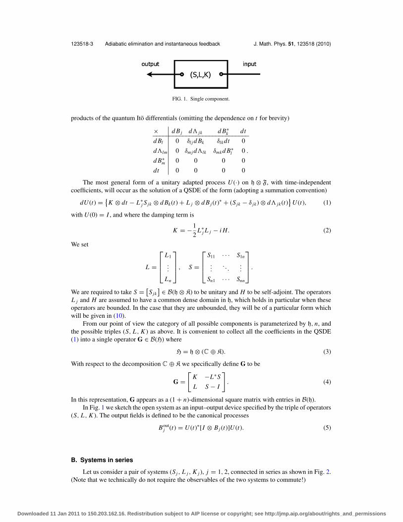
123518-3 Adiabatic elimination and instantaneous feedback J. Math. Phys. 51, 123518 (2010)
FIG. 1. Single component.
products of the quantum Ito differentials (omitting the dependence on t for brevity)
× d B j d� jk d B∗k dt
d Bl 0 δl j d Bk δlkdt 0
d�lm 0 δmj d�lk δmkd B∗l 0
d B∗m 0 0 0 0
dt 0 0 0 0
.
−−−−−−−−−−−−−−−−−−−−−−−−−−−−−
The most general form of a unitary adapted process U (·) on h ⊗ F, with time-independentcoefficients, will occur as the solution of a QSDE of the form (adopting a summation convention)
dU (t) = {K ⊗ dt − L∗
j S jk ⊗ d Bk(t) + L j ⊗ d B j (t)∗ + (Sjk − δ jk) ⊗ d� jk(t)
}U (t), (1)
with U (0) = I , and where the damping term is
K = −1
2L∗
j L j − i H. (2)
We set
L =
⎡⎢⎢⎣
L1
...
Ln
⎤⎥⎥⎦ , S =
⎡⎢⎢⎣
S11 · · · S1n
.... . .
...
Sn1 · · · Snn
⎤⎥⎥⎦ .
We are required to take S = [Sjk
] ∈ B(h ⊗ K) to be unitary and H to be self-adjoint. The operatorsL j and H are assumed to have a common dense domain in h, which holds in particular when theseoperators are bounded. In the case that they are unbounded, they will be of a particular form whichwill be given in (10).
From our point of view the category of all possible components is parameterized by h, n, andthe possible triples (S, L , K ) as above. It is convenient to collect all the coefficients in the QSDE(1) into a single operator G ∈ B(H) where
H = h ⊗ (C ⊕ K). (3)
With respect to the decomposition C ⊕ K we specifically define G to be
G =[
K −L∗S
L S − I
]. (4)
In this representation, G appears as a (1 + n)-dimensional square matrix with entries in B(h).In Fig. 1 we sketch the open system as an input–output device specified by the triple of operators
(S, L , K ). The output fields is defined to be the canonical processes
Boutj (t) = U (t)∗[I ⊗ B j (t)]U (t). (5)
B. Systems in series
Let us consider a pair of systems (Sj , L j , K j ), j = 1, 2, connected in series as shown in Fig. 2.(Note that we technically do not require the observables of the two systems to commute!)
Downloaded 11 Jan 2011 to 150.203.162.16. Redistribution subject to AIP license or copyright; see http://jmp.aip.org/about/rights_and_permissions

123518-4 Gough, Nurdin, and Wildfeuer J. Math. Phys. 51, 123518 (2010)
FIG. 2. Systems in series.
In the instantaneous feedforward limit, the pair can be viewed as the single system shown inFig. 3 with overall parameters5
(Sser, Lser, Kser) = (S2, L2, K2) � (S1, L1, K1), (6)
where the series product � is the associative (though noncommutative) product given by the explicitidentification
Sser = S2S1, (7)
Lser = L2 + S2L1, (8)
Kser = K1 + K2 − L∗2 S2L1. (9)
Note that if Hj ( j = 1, 2) are the Hamiltonians of the separate systems then the dampingoperators are K j = − 1
2 L∗j L j − i Hj and the effective Hamiltonian in series is then given by
Hser = H1 + H2 + Im(L∗2 S2L1).
C. Adiabatic elimination of oscillators
We suppose that the system consists of local oscillators having Hilbert space hosc and that theremaining degrees of freedom live on an auxiliary space h. The overall Hilbert space of the systemis then h ⊗ hosc and we consider an open model described by the triple of operators
S(k) = S ⊗ I,
L(k) = k∑
j
C j ⊗ a j + G ⊗ I,
K (k) = k2∑
jl
A jl ⊗ a∗j al + k
∑j
Z j ⊗ a∗j + k
∑j
X j ⊗ a j + R ⊗ I, (10)
FIG. 3. Systems in series: the upper setup describes two systems connected in series with a time lag τ > 0 in the intercon-nection from system 1 to 2. In the instantaneous feedforward (I.F.) limit we consider τ → 0 in which case we obtain aneffective single component model again.
Downloaded 11 Jan 2011 to 150.203.162.16. Redistribution subject to AIP license or copyright; see http://jmp.aip.org/about/rights_and_permissions

123518-5 Adiabatic elimination and instantaneous feedback J. Math. Phys. 51, 123518 (2010)
FIG. 4. The setup on the left shows a system of an oscillator and auxiliary component with the oscillator coupled to a quantumfield input. In the limit where the coupling of the oscillator becomes infinitely strong, we may adiabatically eliminate theoscillator to obtain an input acting directly on the auxiliary component. This is sketched in the setup on the right.
where k is a positive scaling parameter and S, C j , G, A jl , X j , Z j , R are bounded operators on h withA = [
A jl]
boundedly invertible. Here a j is the annihilator corresponding to the j th local oscillator,say with j = 1, · · · , m.
As k → ∞ the oscillators become increasingly strongly coupled to the driving noise field andin this limit we would like to consider them as being permanently relaxed to their joint groundstate. The oscillators are then the fast degrees of freedom of the system, with the auxiliary space h
describing the slow degrees. In the adiabatic elimination k → ∞ we desire a reduced descriptionof an open system involving the operators of h only, with the fast oscillators being eliminated, asillustrated in Fig. 4. The ground state for the ensemble of m oscillators will be denoted by |0〉osc.
Define X to be the row vector of operators X = (X1, X2, . . . , Xm) and Z to be the columnvector of operators Z = (Z1, Z2, . . . , Zm)T . Also, we say that a matrix M = [M jl] j,l=1,...,m , withM jl bounded operators on h, is strictly Hurwitz stable if Re〈φ, Mφ〉 < 0 for all 0 = φ ∈ h ⊗ Cm .Then we say that an open Markov quantum system with parameters of the form (10) is strictlyHurwitz stable if the matrix [A jl] is strictly Hurwitz stable. We first have the following result:
Theorem 1: Let U (·, k) be the unitary adapted evolution associated with the triple (S(k), L(k), K (k))appearing in (10), and define the slow space as hs = h ⊗ {C |0〉osc}. If the operator Y = ∑
jl A jl ⊗a∗
j al has kernel space equal to the slow space, then we have the limit
limk→∞
sup0≤t≤T
∥∥U (t, k)� − U (t)�∥∥ = 0,
for all T > 0 and � ∈ hs ⊗ F, where U (·) is the unitary evolution associated with the triple S ⊗|0〉〈0|osc, L ⊗ |0〉〈0|osc, K ⊗ |0〉〈0|osc and
S = (I + C A−1C∗)S,
L = G − C A−1 Z ,
K = R − X A−1 Z . (11)
Remark 2: For ease of notation, we will drop the factor “· ⊗ |0〉〈0|osc” as it is obvious that in thelimit we are always relaxed into the fast oscillator ground states. Therefore we can simply think ofthe limit QSDE as having initial space h and coefficients (S, L, K ).
Remark 3: A sufficient, though not necessary, condition for the kernel space of Y to equal the slowspace is that the matrix A be strictly Hurwitz, see Lemma 15.
The result is a generalization of what has been established for the single mode case11 wherethe main result is stated for weak convergence of the unitaries, but this automatically extends to thestrong convergence above. There the techniques were based on a quantum central limit theorem14
which have been shown to extend to the multimode situation.15 We shall give a proof of the theoremin the Appendix, exploiting the theory of singular perturbation of QSDEs developed by Boutenet al.13
Downloaded 11 Jan 2011 to 150.203.162.16. Redistribution subject to AIP license or copyright; see http://jmp.aip.org/about/rights_and_permissions
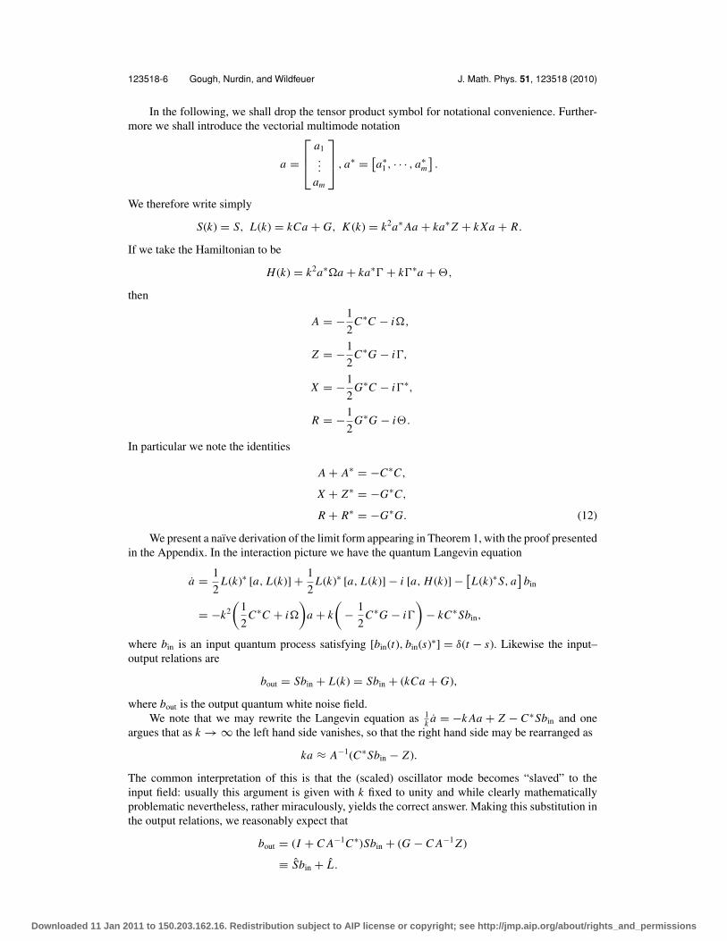
123518-6 Gough, Nurdin, and Wildfeuer J. Math. Phys. 51, 123518 (2010)
In the following, we shall drop the tensor product symbol for notational convenience. Further-more we shall introduce the vectorial multimode notation
a =
⎡⎢⎣
a1...
am
⎤⎥⎦ , a∗ = [
a∗1 , · · · , a∗
m
].
We therefore write simply
S(k) = S, L(k) = kCa + G, K (k) = k2a∗ Aa + ka∗ Z + k Xa + R.
If we take the Hamiltonian to be
H (k) = k2a∗�a + ka∗� + k�∗a + ,
then
A = −1
2C∗C − i�,
Z = −1
2C∗G − i�,
X = −1
2G∗C − i�∗,
R = −1
2G∗G − i.
In particular we note the identities
A + A∗ = −C∗C,
X + Z∗ = −G∗C,
R + R∗ = −G∗G. (12)
We present a naıve derivation of the limit form appearing in Theorem 1, with the proof presentedin the Appendix. In the interaction picture we have the quantum Langevin equation
a = 1
2L(k)∗ [a, L(k)] + 1
2L(k)∗ [a, L(k)] − i [a, H (k)] − [
L(k)∗S, a]
bin
= −k2
(1
2C∗C + i�
)a + k
(− 1
2C∗G − i�
)− kC∗Sbin,
where bin is an input quantum process satisfying [bin(t), bin(s)∗] = δ(t − s). Likewise the input–output relations are
bout = Sbin + L(k) = Sbin + (kCa + G),
where bout is the output quantum white noise field.We note that we may rewrite the Langevin equation as 1
k a = −k Aa + Z − C∗Sbin and oneargues that as k → ∞ the left hand side vanishes, so that the right hand side may be rearranged as
ka ≈ A−1(C∗Sbin − Z ).
The common interpretation of this is that the (scaled) oscillator mode becomes “slaved” to theinput field: usually this argument is given with k fixed to unity and while clearly mathematicallyproblematic nevertheless, rather miraculously, yields the correct answer. Making this substitution inthe output relations, we reasonably expect that
bout = (I + C A−1C∗)Sbin + (G − C A−1 Z )
≡ Sbin + L.
Downloaded 11 Jan 2011 to 150.203.162.16. Redistribution subject to AIP license or copyright; see http://jmp.aip.org/about/rights_and_permissions

123518-7 Adiabatic elimination and instantaneous feedback J. Math. Phys. 51, 123518 (2010)
FIG. 5. The picture illustrates the main result that we wish to prove here, namely, the adiabatic elimination (A.E.) and theinstantaneous feedforward (I.F.) limits can be interchanged.
This justifies the form of S and L . The form of K may be deduced by substituting ka ≈ A−1(C∗Sbin −Z ), and the conjugate relation, into the Langevin equation for any operator acting nontrivially onlyon the space h. (There is a potential operator ordering ambiguity here, and the appropriate choice isto substitute ka and ka∗ in Wick ordered form!)
D. Adiabatic elimination and systems in series
The aim of this section is to determine whether the limits of adiabatic elimination and instan-taneous feedforward do in fact commute, as illustrated in Fig. 5. While this is often assumed inquantum optics models, it is certainly far from obvious. At this stage, however, we are able to reducethe question to a direct computation.
Let us represent the local oscillators a1 and a2 in a combined manner as
a =[
a1
a2
].
Then the first system is to be represented as (S1(k), L1(k), K1(k)) where
S1(k) = S1,
L1(k) = kC1a1 + G1 ≡ k[C1, 0]a + G1,
K1(k) = k2a∗1 A1a1 + ka∗
1 Z1 + k Xa1 + R1
≡ k2a∗[
A1 0
0 0
]a + ka∗
[Z1
0
]+ k [X1, 0] a + R1.
Likewise, the second system is then represented as
S2(k) = S2,
L2(k) ≡ k[0, C2]a + G2,
K2(k) ≡ k2a∗[
0 0
0 A2
]a + ka∗
[0
Z2
]+ k [0, X2] a + R2.
Downloaded 11 Jan 2011 to 150.203.162.16. Redistribution subject to AIP license or copyright; see http://jmp.aip.org/about/rights_and_permissions

123518-8 Gough, Nurdin, and Wildfeuer J. Math. Phys. 51, 123518 (2010)
1. Adiabatic elimination followed by instantaneous feedforward
If we perform the adiabatic elimination first then we arrive at the two systems ( j = 1, 2)
S j = (I + C j A−1j C∗
j )Sj
L j = G j − C j A−1j Z j ,
K j = R j − X j A−1j Z j .
The instantaneous feedforward limit is then given by the series product
S = S2 S1,
L = L2 + S2 L1,
K = K1 + K2 − L∗2 S2 L1. (13)
2. Instantaneous feedfoward followed by adiabatic elimination
We perform the series product (S2(k), L2(k), K2(k)) � (S1(k), L1(k), K1(k)) first to obtain(Sser(k), Lser(k), Kser(k)) where
Sser(k) = S2S1,
Lser(k) = L2(k) + S2L1(k)
≡ k[S2C1, C2]a + G1 + S2G1,
Kser(k) = K1(k) + K2(k) − L2(k)∗S2(k)L1(k)
= k2a∗[
A1 0
−C∗2 S2C1 A2
]a + ka∗
[Z1
Z2 − C∗2 S2G1
]
+ k[X1 − G∗
2 S2C1, X2]
a + R1 + R2 − G∗2 S2G1.
Now, adiabatically eliminating the oscillators leads to the effective model (Sser, Lser, Hser). Herewe have
Sser =(
I + [S2C1, C2]
[A1 0
−C∗2 S2C1 A2
]−1 [C∗
1 S∗2
C∗2
] )S2S1,
Lser = (G1 + S2G1) − [S2C1, C2]
[A1 0
−C∗2 S2C1 A2
]−1 [Z1
Z2 − C∗2 S2G1
],
Kser = (R1 + R2 − G∗2 S2G1)
− [X1 − G∗
2 S2C1, X2] [
A1 0
−C∗2 S2C1 A2
]−1 [Z1
Z2 − C∗2 S2G1
]. (14)
E. Commutativity of the limits: Systems in series
The matrix inverse appearing in (14) is easily computed as a special case of the well-knownformula for the inverse of block matrices (the earliest reference is credited to Banachiewicz,8 seeSec. III A, however, like many matrix identities the origins may be considerably older)[
A1 0
−C∗2 S2C1 A2
]−1
=[
A−11 0
A−12 C∗
2 S2C1 A−11 A−1
2
]. (15)
Downloaded 11 Jan 2011 to 150.203.162.16. Redistribution subject to AIP license or copyright; see http://jmp.aip.org/about/rights_and_permissions

123518-9 Adiabatic elimination and instantaneous feedback J. Math. Phys. 51, 123518 (2010)
This yields the explicit form
Sser = (I + S2C1 A−11 C∗
1 S∗2 + C2 A−1
2 C∗2 S2C1 A−1
1 C∗1 S∗
2 + C2 A−12 C∗
2 )S2S1
= (I + C2 A−12 C∗
2 )S2(I + C1 A−11 C∗
1 )S1
≡ S2 S1.
The coupling operator is
Lser = (G1 + S2G1) − S2C1 A−11 Z1
−C2 A−12 C∗
2 S2C1 A−11 Z1 − C2 A−1
2 Z2 + C2 A−12 C∗
2 S2G1
= (G2 − C2 A−12 Z2) + (I + C2 A−1
2 C∗2 )S2(G1 − C1 A−1
1 Z1)
≡ L2 + S2 L1.
Finally we see that
Kser = R1 + R2 − G∗2 S2G1 − X1 A−1
1 Z1
+G∗2 S2C1 A−1
1 Z1 − X2 A−12 Z2 + X2 A−1
2 C∗2 S2(G1 − C1 Z1).
We would like to show that this equals K1 + K2 − L∗2 S2 L1, now we have
K1 + K2 − L∗2 S2 L1 = R1 − X1 A−1
1 Z1 + R2 − X2 A−12 Z2
−(G∗2 − Z∗
2 A−1∗2 C∗
2 )(I + C2 A−12 C∗
2 )S2(G1 − C1 A−11 Z1),
and to compute this we note that A2 = − 12 C∗
2 C2 − i�2 so that
A−1∗2 C∗
2 (I + C2 A−12 C∗
2 ) = A−1∗2 (I + C∗
2 C2 A−12 )C∗
2
= A−1∗2 (A2 + C∗
2 C2)A−12 C∗
2
= A−1∗2 (−A∗
2)A−12 C∗
2
= −A−12 C∗
2 , (16)
this yields
K1 + K2 − L∗2 S2 L1 = R1 − X1 A−1
1 Z1 + R2 − X2 A−12 Z2
−G∗2(I + C2 A−1
2 C∗2 )S2(G1 − C1 A−1
1 Z1)
−Z∗2 A−1
2 C∗2 S2(G1 − C1 A−1
1 Z1).
We therefore find that
Kser − (K1 + K2 − L∗2 S2 L1) = {
X2 + G∗2C2 + Z∗
2
}A−1
2 C∗2 S2(G1 − C1 Z1);
however, this vanishes identically by the second of identities (12).We therefore conclude that the model parameters in (13) are identical with those in (14);
therefore the adiabatic elimination and instantaneous feedforward limit commute.
F. Adiabatic elimination: In-loop device
Next we want to extend our investigation to situations where we have a nontrivial feedbackarrangement as illustrated in Fig. 6. The question again is whether the two limits commute.
We start off with a simple model in-loop, taking the four-port device to be a beam splitter,modeled by a unitary matrix T = [Tjl] with complex entries and where coupling operators and the
Downloaded 11 Jan 2011 to 150.203.162.16. Redistribution subject to AIP license or copyright; see http://jmp.aip.org/about/rights_and_permissions

123518-10 Gough, Nurdin, and Wildfeuer J. Math. Phys. 51, 123518 (2010)
FIG. 6. General feedback arrangement: the four-port device interacts with one external input, producing one external outputand interacts with an in-loop device by one internal input and output field, respectively.
systems Hamiltonian are zero, L1 = L2 = H1 = 0. We parameterize the in-loop device as
S0(k) = S0,
L0(k) = k√
γ a0,
K0(k) = −1
2k2a∗
0γ a0, (17)
and fix the beam splitter (scattering) matrix as (with α real)
T =[
α√
1 − α2√1 − α2 −α
]. (18)
Thus, the in-loop system consists only of a single oscillator coupled to the in-loop field and no ad-ditional modes coupled to the oscillator. In terms of operator parameters S0, C0, G0, A0, Z0, X0, R0,see Eq. (10),
S0(k) = S0 ⊗ I,
L0(k) = kC0 ⊗ a + G0 ⊗ I,
K0(k) = k2 A0 ⊗ a∗a + k Z0 ⊗ a∗ + k X0 ⊗ a + R0 ⊗ I,
acting on the space hsys ⊗ hosc, we see that
S0 = S0,
A0 = −1
2γ,
C0 = √γ ,
Z0 = X0 = R0 = G0 = 0.
The coefficients for the single input single output device after taking the instantaneous feedbacklimit of the arrangement of Fig. 6 were derived by Gough and James4 and are given by
Sred = T11 + T12S0(I − T22S0)−1T21,
L red = T12(I − T22S0)−1L0,
Hred = K0 − L∗0 S0(I − T22S0)−1L0. (19)
For the model (17), the limit coefficients after taking the adiabatic elimination limit (see Theorem1) are given by
S0 = (I + C0 A−1
0 C∗0
)S0 = −S0,
L0 = G0 − C0 A−10 Z0 = 0,
K0 = R0 − X0 A−10 Z0 = 0. (20)
Downloaded 11 Jan 2011 to 150.203.162.16. Redistribution subject to AIP license or copyright; see http://jmp.aip.org/about/rights_and_permissions

123518-11 Adiabatic elimination and instantaneous feedback J. Math. Phys. 51, 123518 (2010)
Substituting into (19) we find that the reduced coefficients after the instantaneous feedback limit forthe model (20) are
S = α +√
1 − α2(−S0)1
1 − (−α)(−S0)
√1 − α2 = α − S0
1 − αS0, (21)
L = 0,
K = 0.
We now exchange the order in which we perform the limits. The instantaneous feedback limitof the model before taking the adiabatic elimination limit yields:
S(k) = T11 + T12S0 (I − T22S0)−1 T21 = α + (1 − α2) S0
1
1 + αS0,
L(k) = k√
1 − α21
1 + αS0
√γ a0,
K (k) = K0(k) − L0(k)∗S0T22
1 − S0T22L0(k) = k2a∗
0
(−1
2γ + γ
αS0
1 + αS0
)a0,
where the operator parameters are
A = −γ
2
1 − αS0
1 + αS0,
C =√
1 − α2√γ
1 + αS0,
S = α +(1 − α2
)S0
1 + αS0,
G = X = Z = R = 0.
The A.E. of the I.F. limit model then results in (here |1 + αS0|2 = (1 + αS∗0 )(1 + αS0))
S =(
1 −(1 − α2
)γ
|1 + αS0|22
γ
1 + αS0
1 − αS0
) (α + (1 − α2)S0
1 + αS0
)
=(αS∗
0 − 1)
(1 + αS0)(1 + αS∗
0
)(1 − αS0)
(α + S0
1 + αS0
)
= α − S0
1 − αS0. (22)
We see that the limits do in fact commute since we obtain the same operator S in (21) and (22),likewise for the operators L and K . The apparently miraculous agreement comes as a general featurethat will be observed in more complex networks. Our approach will be to encode both these limitsas instances of a Schur complement operation: the miraculous agreements that one encounters in acase-by-case study are in fact just by-product of these operations.
If S0 = 1 then in quantum optics the system (S0(k), L0(k), K0(k)) represents a one-sided opticalcavity in which the coupling coefficient k
√γ of the partially transmitting cavity mirror is large
(for large k). The calculations of this section show that for large k the network in Fig. 7 can beconsistently approximated by an effective device that shifts the phase of the output field with respectto the input field by an amount determined by the parameters of the cavity and beam splitter. Alter-natively, one can also think of the network of Fig. 7 as approximately implementing a phase shiftingdevice.
Downloaded 11 Jan 2011 to 150.203.162.16. Redistribution subject to AIP license or copyright; see http://jmp.aip.org/about/rights_and_permissions

123518-12 Gough, Nurdin, and Wildfeuer J. Math. Phys. 51, 123518 (2010)
FIG. 7. Oscillator in-loop.
III. ADIABATIC ELIMINATION WITHIN GENERAL NETWORKS
The situation of two systems in cascade, as depicted in Fig. 2, is the simplest form of a nontrivialquantum feedback network. We remark that at no stage of the calculations did we assume that theoperators describing the first system commuted with those of the second system. Indeed, the seriesproduct is valid even if we do not assume that we are dealing with separate cascaded systems and isapplicable to the problem of feedback into the same system.
In Fig. 8 we describe a somewhat more engorged quantum feedback network featuring feedbackand feedforward interconnections. For each component of the network, we will have the samemultiplicity for the input fields as the output fields, though we split up the inputs and outputsgeometrically to indicate different physical connections for the fields. The unitary S for a givencomponent now additionally implies that we can use the component to mix the input fields, witha beam-splitter being the very special case where the entries of S are just complex constants. Thisfeature introduces the possibility of topologically nontrivial feedback loops that were not present inthe simple situations of direct feedforward or feedback occurring for systems in series.
We now aim to investigate the procedure of adiabatic elimination of fast degrees of freedomfrom components in a general quantum feedback network and, in particular, answer the question ofwhether this commutes with the Markov limit in which we take vanishing time lags for the variousinternal fields in the network. The adiabatic elimination of oscillators for components in series willthen be a very specific case of this general theory.
The essentially mathematical element in the investigation will be that both the adiabatic elimina-tion limit and the instantaneous feedback limit for a general quantum feedback network are actuallyinstances of a Schur complement of the Ito matrix G.
FIG. 8. Quantum feedback network.
Downloaded 11 Jan 2011 to 150.203.162.16. Redistribution subject to AIP license or copyright; see http://jmp.aip.org/about/rights_and_permissions

123518-13 Adiabatic elimination and instantaneous feedback J. Math. Phys. 51, 123518 (2010)
A. The Schur complement
We begin by recalling some of the basic definitions and notations relevant for Schur comple-ments. For general reviews, see the survey article by Ouellette6 or the book chapter by Horn andZhang7. We shall elaborate on several of the well-known results presented in the reviews, largely totake account of the fact that we are dealing with block-partitioned matrices with operator entries. Inparticular, we give some minor technical extensions where we are explicit about the domains, kernelspaces, and image spaces on which the operators act.
The Schur complement of an (n + m) square matrix M =[
A BC D
]relative to the m × m
sub-block A is defined to be
M/A = D − C A−1 B
under the assumption that A is invertible. We note the following elementary formula, due toBanachiewicz,8 for invertible M[
A B
C D
]−1
=[
A−1 + A−1 B (M/A)−1 C A−1 −A−1 B (M/A)−1
− (M/A)−1 C A−1 (M/A)−1
].
Definition 4: A matrix M− is a generalized inverse for a square matrix M if we have M M−M = M.The generalized Schur complement of M = [ A B
C D ] is then defined to be
M/A = D − C A− B. (23)
Lemma 5: The generalized Schur complement M/A is well-defined and independent of the choice ofthe generalized inverse A− so long as we have the following inclusions of image spaces im B ⊆ im Aand kernel spaces ker A ⊆ ker C.
Note that im B ⊆ im A occurs if and only if ker A∗ ⊆ ker B∗. (Recall that the image, or columnspace, of a matrix is the span of its columns, or more generally im (M) = ker (M∗)⊥.)
Lemma 6: For two matrices M and N and some generalized inverse M− of M we have that
M M−N = N if im N ⊂ im M
and
N M−M = N if ker M ⊂ ker N .
For the proofs of these lemmata, see Horn and Zhang7; they are a straightforward consequence ofthe definition of a generalized inverse and the postulated image/kernel inclusions.
The Schur complement and Lemmata 5 and 6 above may be generalized to matrices withoperator entries. Let M be a bounded invertible operator on a Hilbert space H and let us fix adecomposition H = ⊕ j∈IH j for some finite index set I. We denote by x j the component of a vectorx ∈ H in H j , and M jl the block component of M mapping from H j to Hl . For A = {a1, . . . , an} andB = {b1, . . . , bm} nonempty subsets of I we write
xA =
⎡⎢⎢⎣
xa1
...
xam
⎤⎥⎥⎦ , MA,B =
⎡⎢⎢⎣
Ma1b1 · · · Ma1bm
.... . .
...
Manbm · · · Manbm
⎤⎥⎥⎦ .
The single equation Mx = u then corresponds to the coarsest block form MI,IxI = uI. In contrast,the full system of equations
∑l∈I M jl xl = u j gives the finest block form. More generally, we may
examine intermediate partitions. Let A and B be nontrivial (i.e., nonempty, proper) subsets of I thenthe equation Mx = u may be written as[
MA,B MA,B ′
MA′,B MA′,B ′
] [xB
xB ′
]=
[u A
u A′
], (24)
Downloaded 11 Jan 2011 to 150.203.162.16. Redistribution subject to AIP license or copyright; see http://jmp.aip.org/about/rights_and_permissions

123518-14 Gough, Nurdin, and Wildfeuer J. Math. Phys. 51, 123518 (2010)
where A′ denotes the complement of the set A in I, and the inverse relation is[xB
xB ′
]=
[(M−1)B,A (M−1)B,A′
(M−1)B ′,A (M−1)B ′,A′
] [u A
u A′
]. (25)
We now recall the definition of the generalized Schur complement, sometimes also known as theshorted operator, in the case where M need not be invertible.
Definition 7: Let A and B be nontrivial subsets of the index I, and let C be a nontrivial subset ofA, and D be a nontrivial subset of B. Furthermore take |A| = |B| and |C | = |D|. Suppose that thesub-block MC,D possesses a generalized inverse denoted by (MC,D)−, then the Schur complementof MA,B relative to MC,D is defined to be
MA,B/MC,D = MA/C,B/D − MA/C,D(MC,D)−MC,B/D.
In the special case where A = B = J, we shall simply write M/MC,D for MJ,J/MC,D.The generalized Schur complement is well-defined and independent of the choice of generalized
inverse so long as the column space im(MC,B/D) is contained in im(MC,D), and ker(MC,D) iscontained in ker(MA/C,D). In particular, if the conditions of the Lemma 5 are met then we may fixa particular generalized inverse such as the Moore–Penrose inverse. We also remark that we mayreadily extend the above notation to the case where different direct-sum decompositions of H areused for the columns and rows of M.
We shall also require the extension of the Banachiewicz formula to generalized inverses.The proof for finite rank matrix operators is due to Marsaglia and Styan,9 and may be found asTheorem 4.6 in the article of Ouellette.6 In the next lemma, we strengthen this to deal with generalHilbert space operators.
Lemma 8: Let M be partitioned according to M =[
A BC D
]. We suppose that im B ⊆ im A,
ker A ⊆ ker C, and therefore the generalized Schur complement X = M/A = D − C A− B is well-defined and independent of the choice of generalized inverse A− to A. Then the generalized inverseof M is given by
M− =[
A− + A− B X−C A− −A− B X−
−X−C A− X−
].
Proof: We multiply out M M−M in block form. The top left block will be
(M M−M)11 = AA− A + AA− B X−C A− A − B X−C A− A
−AA− B X−C + B X−C
= AA− A + AA− B X−C(A− A − 1) − B X−C(A− A − 1)
= AA− A + (AA− − 1)B X−C(A− A − 1)
= A,
where the last step follows because AA− A = A and (AA− − 1)B = 0 under the assumptions thatim B ⊆ im A. Similarly
(M M−M)12 = B + (AA− − 1)B +(AA− − 1)B X−C A− B(AA− − 1)B X− D
= B,
since under the assumption imB ⊆ imA we have that AA− B = B and so(
AA− − 1)
B = 0;
(M M−M)21 = C + C(A− A − 1) + (C A− B − D)X−C(A− A − 1)
= C,
Downloaded 11 Jan 2011 to 150.203.162.16. Redistribution subject to AIP license or copyright; see http://jmp.aip.org/about/rights_and_permissions

123518-15 Adiabatic elimination and instantaneous feedback J. Math. Phys. 51, 123518 (2010)
because of the assumption ker A ⊆ ker C we have C A− A = C and C(A− A − 1) = 0; and
(M M−M)22 = D − (D − C A− B) − (D − C A− B)X−(D − C A− B)
= D − X + X X− X
= D,
since X = M/A = D − C A− B and X X− X = X . Collecting these results we have that M M−M =M , as required. �
Now, as a corollary to Lemma 8 we obtain the generalized Banachiewicz formula:
M−B,A = M−
A,B + M−A,B MA,B ′(M/MA,B)−MA′,B M−
A,B,
M−B,A′ = −M−
A,B MA,B ′(M/MA,B)−,
M−B ′,A = −(M/MA,B)−MA′,B M−
A,B,
M−B ′,A′ = (M/MA,B)−.
We now wish to establish the property of commutativity of successive Schur complementationas this shall be the main technical result required in this paper.
Lemma 9 (Successive complementation rule): Suppose that A, B, C is a partition of the index setI (that is, A, B, C are disjoint nonempty subsets whose union is J) then, whenever the generalizedSchur complements are well-defined, we have the rule
M/MB∪C,B∪C = (M/MC,C )/(M/MC,C )B,B
= (M/MB,B)/((M/MB,B))C,C . (26)
For the case of matrices over a field where the inverses exist, the first equality in (26) is aninstance of the Crabtree–Haynsworth quotient formula6. The extension of the quotient formulato generalized inverses for matrices over a field was given by Carson et al.10 under some rankconditions, see Theorem 4.8 in the review by Ouellete6. However, since here we are dealing withmatrices with Hilbert space operator entries rather than just matrices over a field, we need to extendthis result accordingly. To this end, below we independently prove a generalization of the algebraiccontent of the theorem to matrices with Hilbert space operator entries, modulo the conditions forthese Schur complements to be well-defined which we defer to Lemma 17 in the Appendix.
Proof: Assume that the conditions of Lemma 17 are in place. Let us first compute(M/MC,C )/(M/MC,C )B,B :
M/MC,C =
⎡⎢⎣
MA,A MA,B MA,C
MB,A MB,B MB,C
MC,A MC,B MC,C
⎤⎥⎦ /MC,C
=[
MA,A MA,B
MB,A MB,B
]−
[MA,C
MB,C
](MC,C )− [MC,A MC,B]
= [ML ,R − ML ,C (MC,C )−MC,R
]R,L∈{A,B}
so a second Schur complementation leads to
(M/MC,C )/(M/MC,C )B,B = MA,A − MA,C (MC,C )−MC,A
−(MA,B − MA,C (MC,C )−MC,B)�(MB,A − MB,C (MC,C )−MC,A),
Downloaded 11 Jan 2011 to 150.203.162.16. Redistribution subject to AIP license or copyright; see http://jmp.aip.org/about/rights_and_permissions
123518-16 Gough, Nurdin, and Wildfeuer J. Math. Phys. 51, 123518 (2010)
where we write � = (MB,B − MB,C (MC,C )−MC,B)− for shorthand. We then compute M/MB∪C,B∪C
M/MB∪C,B∪C =
⎡⎢⎣
MA,A MA,B MA,C
MB,A MB,B MB,C
MC,A MC,B MC,C
⎤⎥⎦ /
[MB,B MB,C
MC,B MC,C
]
= MAA − [MA,B MA,C
] [MB,B MB,C
MC,B MC,C
]− [MB,A
MC,A
];
however, the inverse can be computed explicitly using the Banachiewicz formula as[� −�MB,C (MC,C )−
−(MC,C )−MC,B� (MC,C )− + (MC,C )−MC,B�MB,C (MC,C )−
].
Multiplying out the block matrix readily leads to the same expression already obtained for(M/MC,C )/(M/MC,C )B,B . The second equality in (26) follows from Lemma 17 and by interchangingB and C .
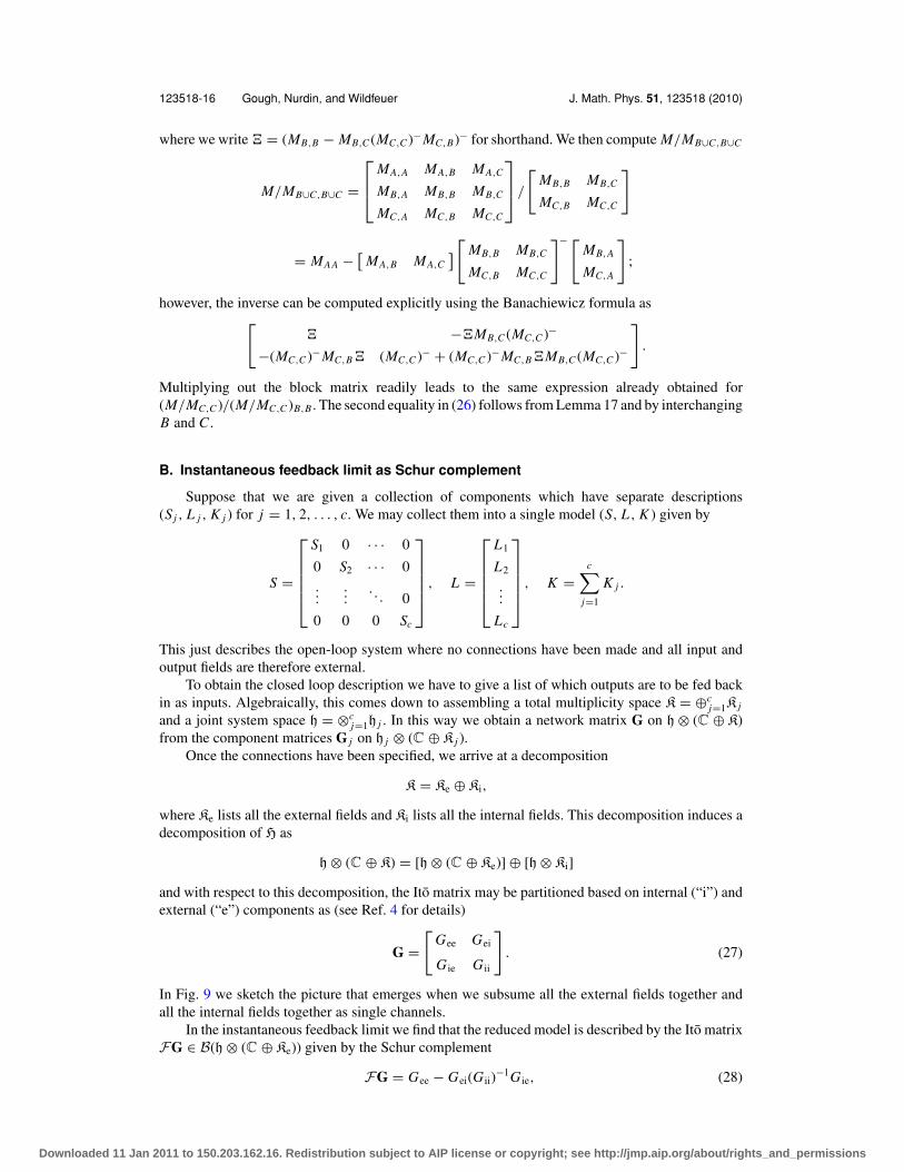
B. Instantaneous feedback limit as Schur complement
Suppose that we are given a collection of components which have separate descriptions(Sj , L j , K j ) for j = 1, 2, . . . , c. We may collect them into a single model (S, L , K ) given by
S =
⎡⎢⎢⎢⎢⎣
S1 0 · · · 0
0 S2 · · · 0...
.... . . 0
0 0 0 Sc
⎤⎥⎥⎥⎥⎦ , L =
⎡⎢⎢⎢⎢⎣
L1
L2
...
Lc
⎤⎥⎥⎥⎥⎦ , K =
c∑j=1
K j .
This just describes the open-loop system where no connections have been made and all input andoutput fields are therefore external.
To obtain the closed loop description we have to give a list of which outputs are to be fed backin as inputs. Algebraically, this comes down to assembling a total multiplicity space K = ⊕c
j=1K j
and a joint system space h = ⊗cj=1h j . In this way we obtain a network matrix G on h ⊗ (C ⊕ K)
from the component matrices G j on h j ⊗ (C ⊕ K j ).Once the connections have been specified, we arrive at a decomposition
K = Ke ⊕ Ki,
where Ke lists all the external fields and Ki lists all the internal fields. This decomposition induces adecomposition of H as
h ⊗ (C ⊕ K) = [h ⊗ (C ⊕ Ke)] ⊕ [h ⊗ Ki]
and with respect to this decomposition, the Ito matrix may be partitioned based on internal (“i”) andexternal (“e”) components as (see Ref. 4 for details)
G =[
Gee Gei
G ie G ii
]. (27)
In Fig. 9 we sketch the picture that emerges when we subsume all the external fields together andall the internal fields together as single channels.
In the instantaneous feedback limit we find that the reduced model is described by the Ito matrixFG ∈ B(h ⊗ (C ⊕ Ke)) given by the Schur complement
FG = Gee − Gei(G ii)−1G ie, (28)
Downloaded 11 Jan 2011 to 150.203.162.16. Redistribution subject to AIP license or copyright; see http://jmp.aip.org/about/rights_and_permissions

123518-17 Adiabatic elimination and instantaneous feedback J. Math. Phys. 51, 123518 (2010)
FIG. 9. Feedback situation.
provided that G ii exists. We remark that the original version of this formula4 involved the related
model matrix U =[
K −L∗SL S
]rather than G and the corresponding feedback reduction map was
the fractional linear transformation FU = Uee + Uei(1 − Uii)−1Uie. In both cases, the condition thatG ii = Sii − I be invertible is necessary for the feedback network to be well-posed.
Remark 10: We note that models studied here all satisfy a Hurwitz stability condition, though notnecessarily in the strict sense. In general, the feedback reduction need not preserve the strictlyHurwitz property, and we may obtain conditionally stable modes through interconnection.
C. Adiabatic elimination as Schur complement
We now re-examine the adiabatic elimination of oscillators. For finite k we consider the Itomatrix
G (k) =[
K (k) −L (k)∗ S
L (k) S − I
],
where we write the scaled operators (10) as
K (k) = [I, ka∗] [
R X
Z A
] [I
ka
],
L (k) = [I, ka∗]
[G C
0 0
] [I
ka
],
S = [I, ka∗]
[S 0
0 0
] [I
ka
].
Recalling Remark 2, it is now convenient to use the decomposition h = h ⊕ h f (here h f denotes thesubspace of the fast oscillator modes) to write
h ⊗ (C ⊕ K) = [h ⊗ (C ⊕ K)
] ⊕ [h f ⊗ (C ⊕ K)
]and with respect to this decomposition we may now write
G (k) = k2a∗g f f a + ka∗g f s + kgs f a + gss
= [I, ka∗]
[gss gs f
g f s g f f
] [I
ka
](29)
Downloaded 11 Jan 2011 to 150.203.162.16. Redistribution subject to AIP license or copyright; see http://jmp.aip.org/about/rights_and_permissions

123518-18 Gough, Nurdin, and Wildfeuer J. Math. Phys. 51, 123518 (2010)
and we set
g =[
gss gs f
g f s g f f
]. (30)
It is easy to see that g is given by
gss =[
R −G∗SG S − I
], gs f =
[X 0C 0
],
g f s =[
Z −C∗S0 0
], g f f =
[A 00 0
].
The Ito matrix corresponding to the limit operators (S, L, K ) in (11) is then
G =[
K −L∗ SL S
]=
[R − X A−1 Z −G∗S + X A−1C∗SG − C A−1 Z S + C A−1C∗S
],
where we use the identity −L∗ S = −G∗S + X A−1C∗S in the upper right corner which relies onthe trick (16) along with the identities (12). We then observe that
G ≡ gss − gs f(g f f
)−g f s = g/g f f
which is the generalized Schur complement based on the Moore–Penrose inverse[A 00 0
]−=
[A−1 00 0
].
Indeed, given the specific form here we see from the remarks after the Definition 7 that anygeneralized inverse may be used here. We may then define the adiabatic elimination operator asA : G (k) �→ G = g/g f f .
IV. COMMUTATIVITY OF THE LIMITS IN GENERAL NETWORKS
Our first step is to see how the instantaneous feedback limit sits with the adiabatic limit startingfrom a general model with fast oscillators and internal connections which we wish to eliminate.
We have seen from (29) that the Ito matrix G (k) may be written as G (k) = [I, ka∗]g
[I
ka
]with g given by (30). Suppose that the input fields can be partitioned into internal and external fieldsthat corresponds to a partitioning of S as
S =[
See Sei
Sie Sii
],
where Sii is a square matrix pertaining to the scattering of the internal fields to themselves, See is asquare matrix pertaining to the scattering of the external fields to themselves, while Sei and Sie pertainto a scattering of internal fields to external fields, and vice versa, respectively. We also partition Cand G accordingly as
C =[
Ce
Ci
]; G =
[Ge
G i
].
If we wish to decompose this with respect to the external and internal field labels, then we obtain
G (k) ≡[
Gee (k) Gei (k)
G ie (k) G ii (k)
]
Downloaded 11 Jan 2011 to 150.203.162.16. Redistribution subject to AIP license or copyright; see http://jmp.aip.org/about/rights_and_permissions

123518-19 Adiabatic elimination and instantaneous feedback J. Math. Phys. 51, 123518 (2010)
similar to (27). We note that these blocks will necessarily have the following structure
Gee (k) ≡ [I, ka∗]gee
[I
ka
],
Gei (k) ≡ [I, ka∗]gei,
G ie (k) ≡ gee
[I
ka
],
G ii (k) = gii,
with
gee =[
R1 M1
G1 Sii − I
]; gei =
[X1 0
Ci 0
];
gie =[
Z1 −C∗Si
0 0
]; gii =
[A 0
0 0
],
and
Se =[
See
Sie
], Si =
[Sei
Sii
], R1 =
[R −G∗Se
Ge See − I
], M1 =
[−G∗Si
Sei
],
G1 = [G i Sie
], Z1 = [
Z −C∗Se], X1 =
[X
Ce
].
We therefore obtain the feedback reduction
FG (k) = Gee (k) ≡ [I, ka∗] (g/gii)
[I
ka
].
Conversely, the adiabatic elimination corresponds to
AG (k) = g/g f f .
In this way we see that the essential action is a Schur complementation of the object g either withrespect to labels of the fast oscillators of the system, or the labels of the internal fields. To this end,we can now establish the main technical result of this paper.
Theorem 11: Let G (k) and FG (k) correspond to strictly Hurwitz stable open quantum systems(i.e., the A matrix of each system is strictly Hurwitz stable), and suppose that Sii + Ci A−1C∗Si − Iand Sii − I are invertible. Then in the notation established above we have
AFG (k) = FAG (k) .
The proof of the above theorem is given in the Appendix. Thus we establish that if G (k) andFG (k) are strictly Hurwitz stable systems, and Sii + Ci A−1C∗Si − I and Sii − I are invertible,the operation of adiabatic elimination of the oscillators in the network indeed commutes with theoperation of taking the instantaneous feedback limit. For the systems in series example of Sec. II Dit can be seen that the strictly Hurwitz stable property holds when A1 and A2 are strictly Hurwitzstable, while for the beam splitter with an in-loop device of Sec. II F it holds when |α| < 1.
The requirement that G (k) and FG (k) be strictly Hurwitz is due to Remark 10. Note that thestrict Hurwitz condition is not however necessary and that the limits may more generally commutewhenever the kernel property of Y in Theorem 1 holds.
Downloaded 11 Jan 2011 to 150.203.162.16. Redistribution subject to AIP license or copyright; see http://jmp.aip.org/about/rights_and_permissions

123518-20 Gough, Nurdin, and Wildfeuer J. Math. Phys. 51, 123518 (2010)
V. CONCLUSION
In this paper we have studied the question of commutativity of adiabatic elimination of oscilla-tory components and the operation of taking the instantaneous feedback limit in a quantum networkwith Markovian components. Provided some mild conditions are satisfied, we answer the questionin the affirmative by showing that adiabatic elimination can be viewed as a Schur complementationoperation, thus putting it on the same footing as the instantaneous feedback limit, and subsequentlyproving the commutativity of successive Schur complementation. This result is important from apractical point of view because in practice it is much easier to obtain a simplified description of aquantum network by first obtaining simplified component models and then using them to obtain adescription of the network rather than the converse operation of first forming the (possibly large)network and applying adiabatic elimination at the network level. Since we have shown that the orderin which adiabatic elimination and the instantaneous feedback limit is taken is inconsequential,this justifies employing the former order of operations which is free of any concerns regarding theuniqueness of the resulting simplified network model in which the fast oscillatory components havebeen eliminated.
ACKNOWLEDGMENTS
J. Gough and H. Nurdin acknowledge the support of EPSRC research grant EP/H016708/1“Quantum Control: Feedback Mediated by Channels in Non-classical States.” H. Nurdin also ac-knowledges the support of the Australian Research Council. The authors thank an anonymousreviewer for bringing their attention to survey paper of Ouellette.6
APPENDIX: PROOFS OF THEOREM 1 AND THEOREM 11
1. Proof of Theorem 1
Let us set
MN = h ⊗ span{|n〉 :
∑n j = N
},
for N = 0, 1, 2, . . .. In particular, we have the direct sum of orthogonal subspaces h ⊗ hosc =⊕N≥0 MN . Let Ps be orthogonal projection onto the “slow subspace” M0 = hs = h ⊗ C|0〉osc andlet Pf = I − Ps . Recall the hypothesis that ker(Y ) = hs . We first have the following:
Lemma 12: Under the hypothesis ker(Y ) = hs , the subspaces MN are stable under YN = Y |MN ,and we have (
Pf Y Pf)−1 = ⊕N≥1Y −1
N .
Moreover, let |δ j 〉 be the state where the j th mode is in the first excited state and all others are inthe vacuum, then (Y1)−1 ∑
j φ j ⊗ |δ j 〉 = ∑jl
(A−1
)jl φl ⊗ |δ j 〉.
Proof: Stability and invertibility of YN on MN follows directly from the specific form of YN and thefact that Y has kernel space M0. The relation
(Pf Y Pf
)−1 = ⊕N≥1Y −1N follows from the direct sum
decomposition.The remaining identity is easily checked from Y
∑j φ j ⊗ |δ j 〉 = ∑
jl A jlφl ⊗ |δ j 〉 and settingthis equal to
∑j φ j ⊗ |δ j 〉 we deduce that φl = (
A−1)
l j φ j . �Corollary 13: ker(Y ∗) = M0.
Proof: By the preceding lemma we have that hf = Pf h ⊗ hosc is stable under Y . Therefore, forany φ ∈ M0 and ψ ∈ h ⊗ hosc we have that 〈φ, Yψ〉 = 〈φ, Y Pf ψ〉 = 0. It follows that 〈Y ∗φ,ψ〉 =〈φ, Yψ〉 = 0 for all ψ ∈ h ⊗ hosc, thus Y ∗φ = 0 for any φ ∈ M0 and we conclude that M0 ⊆ ker(Y ∗).We now need to show the converse that ker(Y ∗) ⊆ M0 and we will do this by contradiction. To dothis end, suppose that ∃ϕ ∈ Pf h ⊗ hosc with ϕ = 0 such that 〈Y ∗ϕ,ψ〉 = 0 for all ψ ∈ h ⊗ hosc. Itfollows that 〈ϕ, Yψ〉 = 0 and therefore 〈ϕ, Y Pf ψ〉 = 0 for all ψ ∈ h ⊗ hosc. But since hf is stable
Downloaded 11 Jan 2011 to 150.203.162.16. Redistribution subject to AIP license or copyright; see http://jmp.aip.org/about/rights_and_permissions

123518-21 Adiabatic elimination and instantaneous feedback J. Math. Phys. 51, 123518 (2010)
under Y and Y |h f is invertible, it follows that ϕ ∈ hs. But this contradicts the hypothesis that ϕ is anonzero element of h f and therefore we conclude that ker(Y ∗) ⊆ M0. This concludes the proof. �
We now state a sufficient condition for ker(Y ) = M0 = ker(Y ∗). Let us first recall the followingdefinition:
Definition 14: A bounded Hilbert space operator A is strictly Hurwitz stable if
Re〈ψ |Aψ〉 < 0, for all ψ = 0.
Lemma 15: Let A jl ∈ B(h) such that A = [A jl
] ∈ B(h ⊗ Cm) is strictly Hurwitz stable. Then theoperator
Y =∑
jl
A jl ⊗ a∗j al (A1)
on h ⊗ hosc has kernel consisting of vectors of the form φ ⊗ |0〉osc, where φ ∈ h.
Proof: We see that for ψ ∈ h ⊗ hosc
〈ψ |Yψ〉 =∑
jl
〈ψ | (I ⊗ a j)∗ (
A jl ⊗ I)
(I ⊗ al) ψ〉 =∑
jl
〈ψ j | A jl ⊗ I ψl〉
where ψ j = (I ⊗ b j
)ψ . We may decompose ψ j ≡ ∑
n ψ j (n) ⊗ |n〉, where |n〉 is the orthonormalbasis of number states for the oscillators and ψ j (n) ∈ h. Then
〈ψ |Yψ〉 =∑
n
∑jl
〈ψ j (n) | A jl ψl (n)〉
and, for each fixed n, we have∑
jl〈ψ j (n) | A jl ψl (n)〉 ≤ 0 with equality if and only if the ψ j (n) = 0since
[A jl
]is assumed to be strictly Hurwitz. In particular, if we assume that ψ is in the kernel of Y
then we deduce that ψ j (n) = 0 for each n and j = 1, · · · , m. It follows that ψ j = (I ⊗ b j
)ψ = 0
for each j = 1, · · · , m, and this implies that ψ ≡ φ ⊗ |0〉osc for some φ ∈ h as required. �Note, however, that as we shall see below, for Theorem 1 to hold it is enough that ker(Y ) = M0.
Lemma 16: The operator S is unitary and K + K ∗ + L∗ L = 0.
Proof: We first show that I + C A−1C∗ is invertible. Suppose that u ∈ ker(I + C A−1C∗)
u = −C A−1C∗u ⇒ C∗u = −C∗C A−1C∗u ⇒ (I + C∗C A−1
)C∗u = 0
⇒ (A + C∗C
)A−1C∗u = 0 ⇒ −A∗ A−1C∗u = 0 ⇒ C∗u = 0
so substituting C∗u = 0 into u = −C A−1C∗u we see that u = 0, therefore ker S = 0. As S is unitary,we have
S S∗ = (I + C∗ A−1C
) (I + C A∗−1C∗)
= I + C A−1(
A + A∗ + C∗C)
A∗−1C∗ = I
using the first of identities (12). Similarly S∗ S = I .Likewise we use (12) to show that
K + K ∗ + L∗ L = R − X A−1 Z + R∗ − Z∗ A∗−1 X∗
+ (G∗ − Z∗ A∗−1C∗) (
G − C A−1 Z)
= − (X − G∗C
)A−1 Z − Z∗ A∗−1
(X∗ − C∗G − C∗C A−1 Z
)= Z∗ A−1 Z + Z∗ A∗−1 (
Z + C∗C A−1 Z)
= Z∗ A∗−1(A + A∗ + C∗C)A−1 Z
= 0. �
Downloaded 11 Jan 2011 to 150.203.162.16. Redistribution subject to AIP license or copyright; see http://jmp.aip.org/about/rights_and_permissions

123518-22 Gough, Nurdin, and Wildfeuer J. Math. Phys. 51, 123518 (2010)
Using the above results, we can now proceed to complete the proof of Theorem 1. Let us firstrecall the main results from Bouten et al 13. Let V (t, k) = U (t, k)∗, then V satisfies the left QSDE(using a summation convention)
dV (t, k) = V (t, k){α (k) ⊗ dt + βl (k) ⊗ d Bl (t) + γ j ⊗ d B j (t)
∗ + (ε jl − δ jl) ⊗ d� jl (t)},
where α (k) = k2α2 + kα1 + α0 = K (k)∗, β j (k) = kβ1, j + β0, j = L j (k)∗, γ j (k) = −S∗l j Ll , and
ε jl = S∗l j . Their results are stated for the left QSDE for the reason that it is easier to formulate
the conditions for unbounded coefficients this way; however, the treatment is of course equivalent.We note that α2 is then Y ∗, with kernel space M0, and we denote its Moore–Penrose inverse
by α2 (note that this Moore–Penrose inverse exists since Y ∗ has the same form and properties asY ). The prelimit coefficients satisfy Assumption 1 in the paper of Bouten et al.13 by construction.Assumption 2 of that work corresponds to the identities α2α2 = α2α2 = Pf , α2 Ps = 0, β∗
1,i Ps = 0,and Psα1 Ps = 0: the last three are automatic since Ps projects onto the ground state of the oscillatorand in each case we encounter a j |0〉osc = 0. The limit coefficients in Assumption 3 of Ref. 13 arethen
α = Ps (α0 − α1α2α1) Ps = (R∗ − Z∗ A∗−1 X∗) ⊗ |0〉〈0|osc ≡ K ∗ ⊗ |0〉〈0|osc,
β = Ps (β0 − α1α2β1) Ps = (G∗ − Z∗ A∗−1C∗) ⊗ |0〉〈0|osc ≡ L∗ ⊗ |0〉〈0|osc,
ε = Psε(I + β∗
1 α2β1)
Ps = S∗ (I + C∗ A∗−1C∗) ⊗ |0〉〈0|osc ≡ S∗ ⊗ |0〉〈0|osc,
γ ≡ −εβ∗ ≡ −S∗ L ⊗ |0〉〈0|osc,
with (S, L, K ) as given in the statement of Theorem 1. These coefficients evidently satisfy therequirements of Assumption 3, namely, to generate a unitary adapted Hudson–Parthasarathy equationon a common invariant domain in M0, as was established in Lemma 16. �
2. Conditions for the Schur complements in Lemma 9 to be well-defined
Lemma 17: If
ker
[MB,B MB,C
MC,B MC,C
]⊆ ker [MA,B MA,C ] (A2)
im
[MB,A
MC,A
]⊆ im
[MB,B MB,C
MC,B MC,C
](A3)
ker MC,C ⊆ ker MB,C (A4)
im MC,B ⊆ im MC,C (A5)
ker MB,B ⊆ ker MC,B (A6)
im MB,C ⊆ im MB,B, (A7)
then the Schur complements (M/MC,C )/(M/MC,C )B,B and (M/MB,B)/((M/MB,B))C,C are all well-defined.
Proof: Collecting the Schur complements used in the proof of Lemma 9 (successive complementationrule), we see that we have to show that
M/MC,C , M/MB,B, (M/MC,C )/(M/MC,C )B,B
MA∪C,A∪C/MC,C , MA∪C,B∪C/MC,C , MB∪C,A∪C/MC,C
exist. To proceed, first note that, by Lemma 5, (A2)–(A7) imply that
M/MB∪C,B∪C , MB∪C,B∪C/MB,B, MB∪C,B∪C/MC,C
are well-defined. From ker MB,B ⊆ ker MC,B , we see that MB,B x = 0 ⇒ MC,B x = 0. This com-
bined with condition (A2) shows that MB,B x = 0 ⇒[
MB,B
MC,B
]x = 0 ⇒ MA,B x = 0. Thus (A9),
Downloaded 11 Jan 2011 to 150.203.162.16. Redistribution subject to AIP license or copyright; see http://jmp.aip.org/about/rights_and_permissions

123518-23 Adiabatic elimination and instantaneous feedback J. Math. Phys. 51, 123518 (2010)
given below, holds. Now, (A3) implies that ∀ x ∃ y, z such that[MB,A
MC,A
]x =
[MB,B y + MB,C z
MC,B y + MC,C z
]. (A8)
But conditions (A5) and (A7) imply that ∃ w, v such that MC,B y = MC,Cv and MB,C z = MB,Bw.This together with (A8) shows that im MB,A ⊆ im MB,B and im MC,A ⊆ im MC,C . Combining thiswith (A7) gives us (A10), given below. By analogous arguments we can also establish (A11) and(A12)
ker MB,B ⊆ ker
[MA,B
MC,B
], (A9)
im [ MB,A MB,C ] ⊆ im MB,B, (A10)
ker MC,C ⊆ ker
[MA,C
MB,C
], (A11)
im [MC,A MC,B] ⊆ im MC,C . (A12)
From (A9) to (A12) it follows directly that M/MB,B and M/MC,C exist. Existence ofMA∪C,A∪C/MC,C , MA∪C,B∪C/MC,C , and MB∪C,A∪C/MC,C follows immediately from (A11) and(A12).
Now we show that (M/MC,C )/(M/MC,C )B,B exists. We require
ker(MB,B − MB,C M−C,C MC,B) ⊆ ker(MA,B − MA,C M−
C,C MC,B)
im(MB,A − MB,C M−C,C MC,A) ⊆ im(MB,B − MB,C M−
C,C MC,B)
Let v ∈ im(MB,A − MB,C M−C,C MC,A) be
v = (MB,A − MB,C M−C,C MC,A)x
= [ 1 −MB,C M−C,C ]
[MB,AxMC,Ax
],
for some vector x . Using (A3) and noting that MB,C M−C,C MC,C = MB,C (due to (A4) and
Lemma 6) leads to
v = [ 1 −MB,C M−C,C ]
[MB,B y + MB,C zMC,B y + MC,C z
]
= (MB,B − MB,C M−C,C MC,B)x
which shows the required image space inclusion.To show that ker(MB,B − MB,C M−
C,C MC,B) ⊆ ker(MA,B − MA,C M−C,C MC,B) holds we choose
some x ∈ ker(MB,B − MB,C M−C,C MC,B) and see that
MB,B x − MB,C M−C,C MC,B x = [ MB,B MB,C ]
[x
−M−C,C MC,B x
]= 0
which implies that
[x
−M−C,C MC,B x
]∈ ker[ MB,B MB,C ]. However, MC,B x − MC,C M−
C,C
MC,B x = 0 since MC,C M−C,C MC,B = MC,B (by (A12) and Lemma 6). It then follows that[
x−M−
C,C MC,B x
]∈ ker
[MB,B MB,C
MC,B MC,C
]
which by (A2) implies
[x
−M−C,C MC,B x
]∈ ker [MA,B MA,C ], and therefore we deduce (MA,B
− MA,C M−C,C MC,B)x = 0 which proves the required kernel space inclusion.
Downloaded 11 Jan 2011 to 150.203.162.16. Redistribution subject to AIP license or copyright; see http://jmp.aip.org/about/rights_and_permissions

123518-24 Gough, Nurdin, and Wildfeuer J. Math. Phys. 51, 123518 (2010)
We remark that the conditions (A2)–(A7) are not necessary, as is clear from Horn and Zhang,7
page 42.
3. Proof of Theorem 11
The model may initially be described by the set of coefficients g over the space
H = (h ⊕ h) ⊗ (C ⊕ Ke ⊕ Ki)
and we decompose this as
H = H1 ⊕ H2 ⊕ H3 ⊕ H4
where
H1 = h ⊗ (C ⊕ Ke) , Slow External
H2 = h ⊗ Ki, Slow Internal
H3 = h ⊗ (C ⊕ Ke) , Fast External
H4 = h ⊗ Ki, Fast Internal.
With respect to this decomposition, we decompose g into sub-blocks as
g =
⎡⎢⎢⎢⎣
g11 g12 g13 g14
g21 g22 g23 g24
g31 g32 g33 g34
g41 g42 g43 g44
⎤⎥⎥⎥⎦ ≡
⎡⎢⎢⎢⎣
R1 M1 X1 0
G1 Sii − I Ci 0
Z1 −C∗Si A 0
0 0 0 0
⎤⎥⎥⎥⎦ , (A13)
The set of labels I = {1, 2, 3, 4} can be split up into the slow labels {1, 2} and the fast labelsF = {3, 4} = S′ as well as the external labels E = {1, 3} and the internal labels I = {2, 4} = E ′.
To proceed, we must first establish that the generalized Schur complement is well-defined. Herewe are ultimately retaining the “slow external” degrees of freedom (index 1) and eliminating theindex sets {2, 3, 4}. To this end, We need to check that conditions (A2)–(A7) are all satisfied. Webegin with (A2).
Let (x, y, z)T be an element of
ker
⎡⎣ Sii − I Ci 0
−C∗Si A 00 0 0
⎤⎦ .
Then x, y satisfies (Sii − I )x + Ci y = 0 and −C∗Six + Ay = 0, while z is arbitrary. Therefore, wehave y = A−1C∗Six and (Sii + Ci A−1C∗Si − I )x = 0. Since Sii + Ci A−1C∗Si − I is invertible byhypothesis, we find that x = 0. It then follows that also y = 0, and we conclude that
ker
⎡⎣ Sii − I Ci 0
−C∗Si A 00 0 0
⎤⎦
consists of vectors of the form (0, 0, z)T . Clearly such vectors lie in the kernel of [ M1 X1 0] andwe conclude that
ker
⎡⎣ Sii − I Ci 0
−C∗Si A 00 0 0
⎤⎦ ⊆ ker[ M1 X1 0].
Next, we check if for every given vector x there exist vectors y and z such that we have theequality [
G1x
Z1x
]=
[Sii − I Ci
−C∗Si A
][y
z
]. (A14)
Downloaded 11 Jan 2011 to 150.203.162.16. Redistribution subject to AIP license or copyright; see http://jmp.aip.org/about/rights_and_permissions

123518-25 Adiabatic elimination and instantaneous feedback J. Math. Phys. 51, 123518 (2010)
In particular, this will be satisfied if the matrix[Sii − I Ci
−C∗Si A
]
is invertible. However, since Sii − I + Ci A−1C∗Si and A are invertible we see that this simplyfollows from the Banachiewicz formula. Therefore, for any vector x there indeed exist vectors y andz such that (A14) holds and we conclude that
im
⎡⎢⎣
G1
Z1
0
⎤⎥⎦ ⊆ im
⎡⎢⎣
Sii Ci 0
−C∗Si A 0
0 0 0
⎤⎥⎦ .
Moreover, from the fact that A is invertible we also get
ker
[A 0
0 0
]⊆ ker [ Ci 0 ],
im
[−C∗Si
0
]⊆ im
[A 0
0 0
],
while from the invertibility of Sii − I we automatically have
ker(Sii − I ) ⊆ ker
[−C∗Si
0
],
im [ Ci 0 ] ⊆ im(Sii − I ).
Therefore conditions (A2)–(A7) are satisfied, and the theorem now follows from Lemmata 17and 9.
1 C. Gardiner and P. Zoller, Quantum Noise: A Handbook of Markovian and Non-Markovian Quantum Stochastic Methodswith Applications to Quantum Optics, 2nd ed., Springer Series in Synergetics (Springer, New York, 2000).
2 R. L. Hudson and K. R. Parthasarathy, Commun. Math. Phys. 93, 301 (1984).3 K. Parthasarathy, An Introduction to Quantum Stochastic Calculus (Birkhauser, Berlin, 1992).4 J. Gough and M. R. James, Commun. Math. Phys. 287, 1109 (2009).5 J. Gough and M. R. James, IEEE Trans. Autom. Control 54, 2530 (2009).6 D. V. Ouellette, Linear Algebra Appl 36, 187 (1981).7 R. Horn and F. Zhang, “Basic properties of the Schur complement,” in The Schur Complement and Its Applications, edited
by F. Zhang, Numerical Methods and Algorithms Vol. 4 (Springer, New York, 2005).8 T. Banachiewicz, Acta Astron. 3, 4167 (1937).9 G. Marsaglia and G. P. H. Styan, Sankhya, Ser. A 36, 437 (1974).
10 D. Carlson, E. Haynsworth, and T, Markham, SIAM J. Appl. Math. 26, 169 (1974).11 J. E. Gough and R. van Handel, J. Stat. Phys. 127, 575 (2007).12 L. Bouten and A. Silberfarb, Commun. Math. Phys. 283, 491 (2008).13 L. Bouten, R. van Handel, and A. Silberfarb, J. Funct. Anal. 254, 3123 (2008).14 J. E. Gough, Commun. Math. Phys. 254, 489 (2005).15 J. E. Gough, J. Math. Phys. 47, 113509 (2006).
Downloaded 11 Jan 2011 to 150.203.162.16. Redistribution subject to AIP license or copyright; see http://jmp.aip.org/about/rights_and_permissions


![Index [openresearch-repository.anu.edu.au]](https://img.dokumen.tips/doc/110x75/61dda4703b58a145b1201b55/index-openresearch-.jpg)


