Embed Size (px)
Citation preview

Open Population Mark-Recapture Models
Including Ancillary Sightings
A thesis presented in partial
fulfilment of the requirements
for the degree of
Doctor of Philosophy
in Statistics
at Massey University
Richard J. Barker
1995

Abstract
A model is proposed for a mark-recapture experiment with ancillary observations
obtained from marked animals any time between capture periods and throughout
the geographic range of the animals. The model allows three types of emigration
from the site where recaptures are made: (1) random emigration, where the prob-
ability an animal is at risk of capture at i does not depend on whether it was at
risk of capture at i− 1, (2) permanent emigration where animals can leave the area
where they are at risk of capture but not return, and (3) Markov emigration, where
the probability an animal is at risk of capture at i depends on whether it was at
risk of capture at i − 1. Under random emigration the likelihood function can be
factored into a set of conditionally independent binomial terms used to estimate
the parameters and a set of conditionally independent multihypergeometric terms
that do not involve the parameters. Closed-form maximum likelihood estimators
are derived under random emigration for models with age-dependence and a tem-
porary marking effect. Contingency table based goodness-of-fit tests are derived
from the multihypergeometric terms in the likelihood function. Contingency table
tests of the age-dependence and temporary marking effect models are also derived.
Explicit estimators do not appear to exist for permanent or Markov emigration.
It is shown that the estimator suggested by Jolly (Biometrika 52:239, 1965),
and as a consequence the estimator suggested by Buckland (Biometrics 36:419-435,
1980), is only valid if there is no emigration from the study area or if emigration is
random. The estimator suggested by Mardekian and McDonald (Journal of Wildlife
Management 45:484-488, 1981) for joint analysis of recapture and tag-recovery data
is also only valid under no emigration or random emigration.
By making appropriate constraints on parameters the models reduce to previ-
ously published models including the Jolly-Seber model (with age-dependence and a
temporary marking effect), tag-resight models, tag-recovery models, and joint live-
recapture/tag-recovery models. Thus, the model provides a common framework
for most widely-used mark-recapture models and allows simultaneous analysis of
data obtained in several ways. Advantages of the new models include improved
ii

precision of parameter estimates, and the ability to distinguish between different
type of emigration. FORTRAN programmes are developed for fitting the models
to data with an application to a data set for brown trout (Salmo trutta) tagged in
spawning tributaries of Lake Brunner, Westland between 1987 and 1991.
Acknowledgements
I thank my supervisors Jeff Hunter, Greg Arnold, and Bryan Manly for their help
and encouragement. For support I thank the Statistics Department, Massey Univer-
sity, Hopkins Farming Group and the Hopkins Family Trust, and Manaaki Whenua
- Landcare Research. Special thanks to Jim Nichols for his advice and encourage-
ment. Ken Burnham shared a preprint describing his work in developing a model for
the joint analysis of live-recapture and tag recovery data and excerpts from an un-
published manuscript describing derivation of sampling variances. Also, extensive
comments from Ken Burnham in his examiners report led to many helpful changes
in the final draft. Thanks to my parents Valerie Calder and Les Barker for instill-
ing an academic ambition and especially Lynn, Rachael, James and Anna-Claire
for putting up with this project.
To John,
whose life’s work has made this work possible.
iii

iv

Contents
1 Mark-Recapture Overview 1
1.1 Closed-Population Mark-Recapture Models . . . . . . . . . . . . . . 3
1.1.1 Petersen estimator . . . . . . . . . . . . . . . . . . . . . . . 3
1.1.2 Multiple recaptures . . . . . . . . . . . . . . . . . . . . . . . 4
1.1.3 Generalizations . . . . . . . . . . . . . . . . . . . . . . . . . 6
1.1.4 Log-linear models . . . . . . . . . . . . . . . . . . . . . . . . 10
1.1.5 Martingale estimators . . . . . . . . . . . . . . . . . . . . . 11
1.2 Open Populations . . . . . . . . . . . . . . . . . . . . . . . . . . . 11
1.3 Jolly-Seber Model . . . . . . . . . . . . . . . . . . . . . . . . . . . . 12
1.3.1 Assumptions and notation . . . . . . . . . . . . . . . . . . . 13
1.3.2 Intuitive estimators . . . . . . . . . . . . . . . . . . . . . . 15
1.3.3 The Jolly-Seber likelihood . . . . . . . . . . . . . . . . . . . 16
1.4 Hypergeometric Formulation of the Jolly-Seber Model . . . . . . . . 22
1.4.1 Log-linear models . . . . . . . . . . . . . . . . . . . . . . . . 23
1.4.2 Small sample bias . . . . . . . . . . . . . . . . . . . . . . . . 24
1.4.3 Accuracy of Jolly-Seber variance estimates . . . . . . . . . . 25
1.4.4 Heterogeneous capture and survival probabilities . . . . . . . 26
1.4.5 Special cases of the Jolly-Seber model . . . . . . . . . . . . . 28
1.5 Generalizations of the Jolly-Seber Model . . . . . . . . . . . . . . . 31
1.5.1 Stationary Markov movement model . . . . . . . . . . . . . 35
1.6 General Multi-Strata Movement Models . . . . . . . . . . . . . . . 36
1.6.1 The Petersen estimator for s strata . . . . . . . . . . . . . . 36
v

1.6.2 Open population movement models . . . . . . . . . . . . . . 37
2 Tag Recovery Models 43
2.1 Seber-Robson-Youngs Model . . . . . . . . . . . . . . . . . . . . . . 43
2.1.1 Notation, assumptions, and data structure . . . . . . . . . . 44
2.1.2 Intuitive estimators . . . . . . . . . . . . . . . . . . . . . . . 46
2.1.3 The tag-return model likelihood . . . . . . . . . . . . . . . . 47
2.1.4 Heterogeneous survival and recovery rates . . . . . . . . . . 48
2.1.5 Restricted and generalized tag-return models . . . . . . . . . 50
2.1.6 Models allowing heterogeneous survival . . . . . . . . . . . . 54
2.1.7 Ultrastructural models . . . . . . . . . . . . . . . . . . . . . 55
2.2 Joint Live-Recapture and Tag-Return Models . . . . . . . . . . . . 58
2.2.1 The Mardekian-McDonald analysis . . . . . . . . . . . . . . 58
2.3 Burnham’s Model . . . . . . . . . . . . . . . . . . . . . . . . . . . . 64
2.4 Live-Recapture Analyses Augmented with Sightings . . . . . . . . . 65
3 Single-Stratum Mark-Recapture Models with Ancillary Observa-
tions 67
3.1 Background . . . . . . . . . . . . . . . . . . . . . . . . . . . . . . . 67
3.2 The Experimental Situation, Notation, and Assumptions . . . . . . 68
3.2.1 Notation . . . . . . . . . . . . . . . . . . . . . . . . . . . . . 69
3.2.2 Assumptions . . . . . . . . . . . . . . . . . . . . . . . . . . . 72
3.2.3 Data structure . . . . . . . . . . . . . . . . . . . . . . . . . 73
3.2.4 Random emigration model . . . . . . . . . . . . . . . . . . . 76
3.2.5 The likelihood function under random emigration . . . . . . 82
3.2.6 Parameter estimation . . . . . . . . . . . . . . . . . . . . . . 93
3.2.7 Asymptotic variances and covariances . . . . . . . . . . . . . 95
3.2.8 Goodness-of-fit tests under random emigration . . . . . . . . 99
3.3 Permanent emigration . . . . . . . . . . . . . . . . . . . . . . . . . 105
3.4 Stationary Markov Movement . . . . . . . . . . . . . . . . . . . . . 110
3.5 Losses On Capture . . . . . . . . . . . . . . . . . . . . . . . . . . . 112
vi

3.6 Comparison with Jolly’s Solution . . . . . . . . . . . . . . . . . . . 115
4 Multi-Strata Mark-Recapture Models with Ancillary Observa-
tions 119
4.1 Background . . . . . . . . . . . . . . . . . . . . . . . . . . . . . . . 119
4.2 The Age-Dependence Model . . . . . . . . . . . . . . . . . . . . . . 119
4.2.1 Assumptions, notation and data structure . . . . . . . . . . 120
4.2.2 Random emigration model . . . . . . . . . . . . . . . . . . . 122
4.2.3 Distribution of the MSS . . . . . . . . . . . . . . . . . . . . 129
4.2.4 Maximum likelihood estimators . . . . . . . . . . . . . . . . 136
4.2.5 Asymptotic variances and covariances . . . . . . . . . . . . . 137
4.2.6 Goodness-of-fit tests under random emigration . . . . . . . . 140
4.2.7 Testing for age-dependence . . . . . . . . . . . . . . . . . . . 143
4.2.8 Age-dependent permanent emigration and Markov movement
models . . . . . . . . . . . . . . . . . . . . . . . . . . . . . . 146
4.3 Marking Effect Models . . . . . . . . . . . . . . . . . . . . . . . . . 149
4.3.1 Notation and general model under random emigration . . . . 149
4.3.2 Test for marking effect . . . . . . . . . . . . . . . . . . . . . 156
4.4 Joint Age-Dependence and Marking Effect Model . . . . . . . . . . 157
4.4.1 The probability structure under random emigration . . . . . 158
4.4.2 The likelihood under random emigration . . . . . . . . . . . 159
4.4.3 Parameter estimates . . . . . . . . . . . . . . . . . . . . . . 165
4.5 Observations Obtained After t . . . . . . . . . . . . . . . . . . . . . 170
4.5.1 Probability structure under random emigration . . . . . . . 170
4.5.2 Additional components to the likelihood under random emi-
gration . . . . . . . . . . . . . . . . . . . . . . . . . . . . . . 171
4.5.3 Additional parameter estimates under random emigration . . 174
4.5.4 Additional components to the goodness-of-fit tests . . . . . . 176
4.5.5 Age-dependence and marking effect models under permanent
and Markov emigration with v > t . . . . . . . . . . . . . . 177
vii

5 Modified and Reduced Parameter Models 179
5.1 Models with No Resightings . . . . . . . . . . . . . . . . . . . . . . 179
5.1.1 Benefit of including ancillary observations . . . . . . . . . . 185
5.2 Tag-Resight Model . . . . . . . . . . . . . . . . . . . . . . . . . . . 201
5.3 Tag-Resight when Only Young Animals Are Captured . . . . . . . . 206
5.3.1 Tag-return models . . . . . . . . . . . . . . . . . . . . . . . 207
5.4 Models with Recaptures and 100% Losses on Observation . . . . . . 210
5.5 Fitting Less than Full Rank Models . . . . . . . . . . . . . . . . . . 214
6 Application - Lake Brunner Trout Tagging 1987-1990 219
6.1 One-age Model with no Marking Effect . . . . . . . . . . . . . . . . 220
6.1.1 Females . . . . . . . . . . . . . . . . . . . . . . . . . . . . . 220
6.1.2 Males . . . . . . . . . . . . . . . . . . . . . . . . . . . . . . 222
6.1.3 Comments on the one-age model with no marking effect . . 224
6.2 Age-Dependence and Marking Effect Models . . . . . . . . . . . . . 226
6.2.1 Females . . . . . . . . . . . . . . . . . . . . . . . . . . . . . 226
6.2.2 Males . . . . . . . . . . . . . . . . . . . . . . . . . . . . . . 234
6.3 Discussion . . . . . . . . . . . . . . . . . . . . . . . . . . . . . . . . 250
7 Discussion 253
7.1 Benefits of the New Models and Implications for Existing Methods . 253
7.2 Implication for the Design of New Studies . . . . . . . . . . . . . . 256
7.3 Future Research . . . . . . . . . . . . . . . . . . . . . . . . . . . . . 257
7.3.1 Direct modelling of capture histories . . . . . . . . . . . . . 257
7.3.2 Alternative handling effect models . . . . . . . . . . . . . . . 258
7.3.3 General multi-strata movement model . . . . . . . . . . . . 259
7.3.4 Models with different resighting assumptions . . . . . . . . . 264
7.3.5 Investigations concerning underlying assumptions . . . . . . 265
7.4 Concluding Remarks . . . . . . . . . . . . . . . . . . . . . . . . . . 266
viii

List of Tables
1.1 Reduced m-array summary of a mark-recapture data set with t years
of capture. . . . . . . . . . . . . . . . . . . . . . . . . . . . . . . . . 17
1.2 Probability structure for the reduced m-array of Table 1.1 . . . . . . 18
1.3 Multivariate reduced m-array for a study with t years of capture. . 39
1.4 Multinomial cell probabilities corresponding to the multivariate m-
array of Table 1.3 . . . . . . . . . . . . . . . . . . . . . . . . . . . . 40
2.1 Recovery array for a tag-recovery experiment with 4 years of release
and 6 years of recovery, where Mi,j is the number of tag recoveries
at time j from animals released at time i. . . . . . . . . . . . . . . . 46
2.2 Probability structure for the recovery array in Table 2.1 . . . . . . . 46
2.3 Recovery array for a 2-age tag-recovery experiment with 4 years of
release and 5 years of recovery. . . . . . . . . . . . . . . . . . . . . . 51
2.4 Probability structure for the 2-age tag recovery array of Table 2.3 . 52
2.5 Reduced m-array for a mark-recapture study carried out with t years
of capture and t years of recovery . . . . . . . . . . . . . . . . . . . 64
3.1 Live-recapture reduced m-array for brown trout Salmo trutta cap-
tured and tagged in Lake Brunner 1987-1990 . . . . . . . . . . . . . 67
3.2 Capture history codes -adapted from Pollock et al. (1990). . . . . . 74
3.3 Contributions to the reduced m-array by an animal with capture
history 05013 in a study with t = 5. . . . . . . . . . . . . . . . . . . 75
ix

3.4 Reduced m-array for a mark-recapture study carried out with t years
of capture and ancillary observations of marked animals obtained
during the interval 1, t+ 1. . . . . . . . . . . . . . . . . . . . . . . . 76
3.5 Reduced m-array for a hypothetical t = 4 mark- recapture study
with ancillary observations of animals in the interval i, i + 1. . . . . 77
3.6 Summary statistics for the hypothetical reduced m-array. . . . . . . 77
3.7 Probability structure for animals last released following capture in a
mark-recapture study with t years of capture, ancillary observations
of marked animals obtained during the interval (1, t+1), and random
movement into and out of the area where they are at risk of capture.
In this parameterization p∗i = Fi−1pi and q∗i = 1 − p∗i . . . . . . . . . 79
3.8 Probability structure for animals last released following observation
in a mark-recapture study with t years of capture, ancillary observa-
tions of marked animals obtained during the interval (1, t + 1), and
random movement into and out of the area where they are at risk of
capture. In this parameterization p∗i = Fi−1pi and q∗i = 1 − p∗i , and
δi = 1−θi
θifiρi. . . . . . . . . . . . . . . . . . . . . . . . . . . . . . . . . 80
3.9 Parameter estimates and associated standard errors for the hypo-
thetical mark-recapture data. . . . . . . . . . . . . . . . . . . . . . 95
3.10 Example of a 2× 2 contingency table for the component 1 goodness-
of-fit test . . . . . . . . . . . . . . . . . . . . . . . . . . . . . . . . . 101
3.11 Example of a contingency table for the component 2 goodness-of-fit
test at time i. . . . . . . . . . . . . . . . . . . . . . . . . . . . . . . 103
3.12 Example of a 2× 2 contingency table for the alternative component
2 goodness-of-fit test. This contingency table tests the random em-
igration assumption. Note observed after i includes observed in the
interval i, i+ 1. . . . . . . . . . . . . . . . . . . . . . . . . . . . . . 117
x

4.1 Probability structure under random emigration for age-class 0 ani-
mals last released following capture in a 2-age mark-recapture study
with t years of capture and ancillary observations of marked animals
obtained during the interval (1, t + 1). Note p∗(ν)i = F
(ν)i−1p
(1)i and
q∗(ν)i = 1 − p
∗(ν)i . . . . . . . . . . . . . . . . . . . . . . . . . . . . . . 125
4.2 Probability structure under random emigration for age class 0 an-
imals last released following observation in a 2-age mark-recapture
study with t years of capture, and ancillary observations of marked
animals obtained during the interval (1, t+ 1). Note p∗(ν)i = F
(ν)i−1p
(1)i
and q∗(ν)i = 1 − p
∗(ν)i , and δ
(ν)i =
1−θ(ν)i
θ(ν)i
f(ν)i
ρ(ν)i
. . . . . . . . . . . . . . . 126
4.3 Probability structure under random emigration for age-class 1 ani-
mals last released following capture in a 2-age mark-recapture study
with t years of capture, ancillary observations of marked animals
obtained during the interval (1, t + 1). Note p∗(ν)i = F
(ν)i−1p
(1)i and
q∗(ν)i = 1 − p
∗(ν)i . . . . . . . . . . . . . . . . . . . . . . . . . . . . . . 127
4.4 Probability structure under random emigration for age class 1 an-
imals last released following observation in a 2-age mark-recapture
study with t years of capture, ancillary observations of marked an-
imals obtained during the interval (1, t + 1). Note p∗(ν)i = F
(ν)i−1p
(1)i
and q∗(ν)i = 1 − p
∗(ν)i , and δ
(ν)i =
1−θ(ν)i
θ(ν)i
f(ν)i
ρ(ν)i
. . . . . . . . . . . . . . . 128
4.5 Example of a contingency table for the component 1 goodness-of-fit
test for animals of age l + 1 at time i+ 1 . . . . . . . . . . . . . . . 141
4.6 Example of a contingency table for the component 2 goodness-of-fit
test for animals of age ν at time i (ν < l). . . . . . . . . . . . . . . 144
4.7 Example of a contingency table forming one component of the overall
tests for age-dependence. . . . . . . . . . . . . . . . . . . . . . . . . 146
xi

4.8 Probability structure under random emigration for mark class 0 ani-
mals last released following capture in a mark-recapture study with t
years of capture, ancillary observations of marked animals obtained
during the interval (1, t + 1), and temporary marking effect. Note
p∗(ν)i = F
(ν)i−1p
(ν)i and q
∗(ν)i = 1 − p
∗(ν)i . . . . . . . . . . . . . . . . . . 152
4.9 Probability structure under random emigration for mark class 0 an-
imals last released following observation (in the first resighting in-
terval) in a mark-recapture study with t years of capture, ancil-
lary observations of marked animals obtained during the interval
(1, t+1), and a temporary marking effect. Note p∗(ν)i = F
(ν)i−1p
(ν)i and
q∗(ν)i = 1 − p
∗(ν)i , and δ
(ν)i =
1−θ(ν)i
θ(ν)i
f(ν)i
ρ(ν)i
. . . . . . . . . . . . . . . . . . 153
4.10 Probability structure under random emigration for mark class 1 ani-
mals last released following capture in a mark-recapture study with t
years of capture, ancillary observations of marked animals obtained
during the interval (1, t + 1), and temporary marking effect. Note
p∗(ν)i = F
(ν)i−1p
(ν)i and q
∗(ν)i = 1 − p
∗(ν)i . . . . . . . . . . . . . . . . . . 154
4.11 Probability structure under random emigration for mark class 1 an-
imals last released following observation in a 2-age mark-recapture
study with t years of capture, ancillary observations of marked ani-
mals obtained during the interval (1, t+ 1), and temporary marking
effect. Note p∗(ν)i = F
(ν)i−1p
(ν)i and q
∗(ν)i = 1− p
∗(ν)i , and δ
(ν)i =
1−θ(ν)i
θ(ν)i
f(ν)i
ρ(ν)i
.155
5.1 Probability structure for a t = 4 two-age Jolly-Seber model with no
marking effect under random emigration where p∗(1)i = F
(1)i−1p
(1)i and
p∗(0)i = F
(0)i−1p
(1)i . . . . . . . . . . . . . . . . . . . . . . . . . . . . . . 181
5.2 Probability structure for a t = 4 two-age Jolly-Seber model with no
marking effect under permanent emigration where S∗(ν)i = S
(ν)i F
(ν)i . 182
5.3 Contingency table used to test the “random” vs “permanent” emi-
gration models . . . . . . . . . . . . . . . . . . . . . . . . . . . . . 183
xii

5.4 Average bias of the capture (¯pi − p) and survival (¯Si − S) rate esti-
mators for a t = 5 one-age mark recapture experiment with ancillary
observations and a population made up of high (ph) and low (pl)
capture probability individuals (pl = p − ∆p
2and ph = p + ∆p
2), and
with Si = 0.3. . . . . . . . . . . . . . . . . . . . . . . . . . . . . . . 197
5.5 Average bias of the capture (¯pi − p) and survival (¯Si − S)rate esti-
mators for a t = 5 one-age mark recapture experiment with ancillary
observations and a population made up of high (ph) and low (pl)
capture probability individuals (pl = p − ∆p
2and ph = p + ∆p
2), and
with Si = 0.8. . . . . . . . . . . . . . . . . . . . . . . . . . . . . . . 199
5.6 Probability structure for a t = 4 one-age tag-resight model. All ob-
servations are obtained exactly at sampling time i, and observations
at i of animals released at i ignored. . . . . . . . . . . . . . . . . . . 201
5.7 Probability structure for a t = 4 one-age tag-resight study with a
temporary marking response. For animals released at i, class 0 an-
imals are those animals marked at i and class 1 animals are those
animals marked before i. Note: δ(ν)i =
(1−θ(ν)i
)
θ(ν)i
f(ν)i
. . . . . . . . . . . . 204
5.8 Probability structure for a t = 4 tag-resight study for animals tagged
only as young and with observations obtained throughout the interval
i, i+ 1. Class 0 animals are young, class 1 animals are adult. . . . . 208
5.9 Statistics used by Brownie et al. (1985) for the one-age model with-
out a marking effect and the equivalent ancillary observations model
statistics. . . . . . . . . . . . . . . . . . . . . . . . . . . . . . . . . 209
5.10 Joint live-recapture and tag-recovery array for paradise shelduck
tagged in the Wanganui area 1987-1991. . . . . . . . . . . . . . . . 212
5.11 Summary statistics for Wanganui paradise shelduck tagging program
1987-1991. . . . . . . . . . . . . . . . . . . . . . . . . . . . . . . . . 213
5.12 Parameter estimates for the Wanganui paradise shelduck tagging data213
xiii

5.13 4×2 contingency table testing whether the probability that a member
of r88 is ever captured or recovered is influenced by whether it was
captured in 1988. . . . . . . . . . . . . . . . . . . . . . . . . . . . . 214
6.1 Live-recapture and observation array for female brown trout tagged
in Lake Brunner spawning tributaries, 1987-1990 and observed by
angler captures 1987-1991. . . . . . . . . . . . . . . . . . . . . . . . 220
6.2 Summary statistics for female brown trout tagged in spawning trib-
utaries of Lake Brunner 1987-1990 and observed by anglers 1987-1991.221
6.3 Parameter estimates for female brown trout under the one-age model
with random emigration and no marking effect. . . . . . . . . . . . 221
6.4 Live-recapture and observation array for male brown trout tagged
in Lake Brunner spawning tributaries, 1987-1990 and observed by
angler captures 1987-1991. . . . . . . . . . . . . . . . . . . . . . . . 222
6.5 Summary statistics for male brown trout tagged in spawning tribu-
taries of Lake Brunner 1987-1990 and observed by anglers 1987-1991. 223
6.6 Parameter estimates for male brown trout under the one-age model
with no marking effect. . . . . . . . . . . . . . . . . . . . . . . . . . 223
6.7 Observed and expected values for the 1988 component 2 contingency
table of the random emigration model goodness-of-fit test for males. 225
6.8 Observed and expected values for the 1990 component 2 contingency
table of the random emigration goodness-of-fit test for males. . . . . 225
6.9 Length classes used to assign Lake Brunner brown trout to age-classes.226
6.10 Age-class 0 component of the 4-age reduced m-array with temporary
marking effect for female brown trout tagged in Lake Brunner 1987
- 1990. . . . . . . . . . . . . . . . . . . . . . . . . . . . . . . . . . . 227
6.11 Age-class 1 component of the 4-age reduced m-array with temporary
marking effect for female brown trout tagged in Lake Brunner 1987
- 1990. . . . . . . . . . . . . . . . . . . . . . . . . . . . . . . . . . . 228
xiv

6.12 Age-class 2 component of the 4-age reduced m-array with temporary
marking effect for female brown trout tagged in Lake Brunner 1987
- 1990. . . . . . . . . . . . . . . . . . . . . . . . . . . . . . . . . . . 229
6.13 Age-class 3 component of the 4-age reduced m-array with temporary
marking effect for female brown trout tagged in Lake Brunner 1987
- 1990. . . . . . . . . . . . . . . . . . . . . . . . . . . . . . . . . . . 230
6.14 Summary statistics for age-class 0 female brown trout tagged in
spawning tributaries of Lake Brunner 1987-1990 and observed by
anglers 1987-1991. . . . . . . . . . . . . . . . . . . . . . . . . . . . . 231
6.15 Summary statistics for age-class 1 female brown trout tagged in
spawning tributaries of Lake Brunner 1987-1990 and observed by
anglers 1987-1991. . . . . . . . . . . . . . . . . . . . . . . . . . . . . 232
6.16 Summary statistics for age-class 2 female brown trout tagged in
spawning tributaries of Lake Brunner 1987-1990 and observed by
anglers 1987-1991. . . . . . . . . . . . . . . . . . . . . . . . . . . . . 232
6.17 Summary statistics for age-class 3 female brown trout tagged in
spawning tributaries of Lake Brunner 1987-1990 and observed by
anglers 1987-1991. . . . . . . . . . . . . . . . . . . . . . . . . . . . . 233
6.18 Parameter estimates for age class 0 females in the 4-age model with
temporary marking effect under random emigration. . . . . . . . . . 233
6.19 Parameter estimates for age class 1 females in the 4-age model with
temporary marking effect under random emigration. . . . . . . . . . 234
6.20 Parameter estimates for age class 2 females in the 4-age model with
temporary marking effect under random emigration. . . . . . . . . . 235
6.21 Parameter estimates for age class 3 females in the 4-age model with
temporary marking effect under random emigration. . . . . . . . . . 236
6.22 Parameter estimates, standard errors in parentheses, for age classes
1,2, and 3 from the four age random emigration model with no tem-
porary marking effect for female brown trout tagged in Lake Brunner
1987-1990 . . . . . . . . . . . . . . . . . . . . . . . . . . . . . . . . 237
xv

6.23 Results of contingency table tests for age- dependence and temporary
marking effect. Model 1: no age-dependence and no marking effect;
Model 2a marking effect but no age-dependence; Model 2b: age-
dependence but no marking effect; Model 3: age-dependence and
marking effect. . . . . . . . . . . . . . . . . . . . . . . . . . . . . . 238
6.24 Reduced m-array with temporary marking effect for age-class 0 male
brown trout tagged in Lake Brunner 1987 - 1990. . . . . . . . . . . 239
6.25 Reduced m-array with temporary marking effect for age-class 1 male
brown trout tagged in Lake Brunner 1987 - 1990. . . . . . . . . . . 240
6.26 Reduced m-array with temporary marking effect for age-class 2 male
brown trout tagged in Lake Brunner 1987 - 1990. . . . . . . . . . . 241
6.27 Reduced m-array with temporary marking effect for age-class 3 male
brown trout tagged in Lake Brunner 1987 - 1990. . . . . . . . . . . 242
6.28 Summary statistics for age-class 0 male brown trout tagged in spawn-
ing tributaries of Lake Brunner 1987-1990 and observed by anglers
1987-1991. . . . . . . . . . . . . . . . . . . . . . . . . . . . . . . . . 243
6.29 Summary statistics for age-class 1 male brown trout tagged in spawn-
ing tributaries of Lake Brunner 1987-1990 and observed by anglers
1987-1991. . . . . . . . . . . . . . . . . . . . . . . . . . . . . . . . . 243
6.30 Summary statistics for age-class 2 male brown trout tagged in spawn-
ing tributaries of Lake Brunner 1987-1990 and observed by anglers
1987-1991. . . . . . . . . . . . . . . . . . . . . . . . . . . . . . . . . 244
6.31 Summary statistics for age-class 3 male brown trout tagged in spawn-
ing tributaries of Lake Brunner 1987-1990 and observed by anglers
1987-1991. . . . . . . . . . . . . . . . . . . . . . . . . . . . . . . . . 244
6.32 Parameter estimates for age-class 0 males under the 4-age model
with temporary marking effect under random emigration fitted to
the male data. . . . . . . . . . . . . . . . . . . . . . . . . . . . . . . 245
xvi

6.33 Parameter estimates for age-class 1 males under the 4-age model
with temporary marking effect under random emigration fitted to
the male data. . . . . . . . . . . . . . . . . . . . . . . . . . . . . . . 246
6.34 Parameter estimates for age-class 2 males under the 4-age model
with temporary marking effect under random emigration fitted to
the male data. . . . . . . . . . . . . . . . . . . . . . . . . . . . . . . 247
6.35 Parameter estimates for age-class 3 males under the 4-age model
with temporary marking effect under random emigration fitted to
the male data. . . . . . . . . . . . . . . . . . . . . . . . . . . . . . . 248
6.36 Results of contingency table tests for age- dependence and temporary
marking effect for males. Model 1: no age- dependence and no mark-
ing effect; Model 2a marking effect but no age-dependence; Model
2b: age-dependence but no marking effect; Model 3: age-dependence
and marking effect. . . . . . . . . . . . . . . . . . . . . . . . . . . . 248
6.37 Parameter estimates, standard errors in parentheses, for the age-
independent random emigration model with temporary marking ef-
fect in capture probabilities for male brown trout tagged in Lake
Brunner 1987-1990 . . . . . . . . . . . . . . . . . . . . . . . . . . . 249
7.1 Multivariate reduced m-array for a mark-recapture study beginning
at time 1 with t capture periods and ancillary observations of marked
animals obtained during the interval 1, t+ 1. . . . . . . . . . . . . . 262
7.2 Programme JOLLYOBS Data input for a study of a 2-age population
with temporary trap response where there are 4 years of capture and
4 years of recovery. . . . . . . . . . . . . . . . . . . . . . . . . . . . 280
xvii

xviii

List of Figures
1.1 Overview of the main classes of mark-recapture models and their
inter-relationships. Adapted from Pollock et al. (1990). . . . . . . . 2
5.1 Relative asymptotic efficiency of the survival rate estimator of the
one-age mark recapture model with ancillary observations relative to
the Jolly-Seber model with t = 5 and Si = 0.3 (Relative efficiency =
V ar(SJSi
)
V ar(Si)). . . . . . . . . . . . . . . . . . . . . . . . . . . . . . . . . . 187
5.2 Relative asymptotic efficiency of the survival rate estimator of the
one-age mark recapture model with ancillary observations relative to
the Jolly-Seber model with t = 5 and Si = 0.5 (Relative efficiency =
V ar(SJSi
)
V ar(Si)). . . . . . . . . . . . . . . . . . . . . . . . . . . . . . . . . . 188
5.3 Relative asymptotic efficiency of the survival rate estimator of the
one-age mark recapture model with ancillary observations relative to
the Jolly-Seber model with t = 5 and Si = 0.8 (Relative efficiency =
V ar(SJSi
)
V ar(Si)). . . . . . . . . . . . . . . . . . . . . . . . . . . . . . . . . . 189
5.4 Relative asymptotic efficiency of the survival rate estimator of the
one-age mark recapture model with ancillary observations relative to
the Jolly-Seber model with t = 10 and various survival and capture
probabilities (Relative efficiency =V ar(SJS
i)
V ar(Si)). . . . . . . . . . . . . . 190
xix

5.5 Average asymptotic bias of p∗i relative to the Jolly-Seber model in a
one-age study where the population comprises high (ph) and low (pl)
capture probability individuals. ∆p = ph − pl, t=5, Si = 0.3, and
f = 0.2 (A), 0.4 (B), 0.6 (C), and 0.8 (D). (Relative bias =p∗
i−p
p∗JSi
−p,
P =p). . . . . . . . . . . . . . . . . . . . . . . . . . . . . . . . . . . 193
5.6 Average asymptotic bias of p∗i relative to the Jolly-Seber model in
a one-age study where the population comprises high (ph) and low
(pl) capture probability individual. ∆p = ph − pl, t=5, Si = 0.8, and
f = 0.2 (A), 0.4 (B), 0.6 (C), and 0.8 (D). (Relative bias =p∗
i−p
p∗JSi
−p,
P =p). . . . . . . . . . . . . . . . . . . . . . . . . . . . . . . . . . . 194
5.7 Average asymptotic bias of S∗
i relative to the Jolly-Seber model in
a one-age study where the population comprises high (ph) and low
(pl) capture probability individual. ∆p = ph − pl, t=5, Si = 0.3, and
f = 0.2 (A), 0.4 (B), 0.6 (C), and 0.8 (D). (Relative bias =p∗
i−p
p∗JSi
−p,
P =p). . . . . . . . . . . . . . . . . . . . . . . . . . . . . . . . . . . 195
5.8 Average asymptotic bias of S∗
i relative to the Jolly-Seber model in
a one-age study where the population comprises high (ph) and low
(pl) capture probability individual. ∆p = ph − pl, t=5, Si = 0.8, and
f = 0.2 (A), 0.4 (B), 0.6 (C), and 0.8 (D). (Relative bias =p∗
i−p
p∗JSi
−p,
P =p). . . . . . . . . . . . . . . . . . . . . . . . . . . . . . . . . . . 196
xx

Chapter 1
Mark-Recapture Overview
Estimates of population size obtained by marking a segment of the population and
recording recaptures at later sampling occasions have a long history. The first
recorded use of this technique has been attributed to Laplace who estimated the
population of France in 1786 by recording the number of births in parishes with
a known population and comparing these with birth registrations for the whole
country (Cormack 1968).
There is an extensive mark-recapture literature with important reviews given
by Cormack (1968,1979), Seber (1982,1986,1992), and Pollock et al. (1990). Mark-
recapture models can be broadly divided into two categories: (A) models for popu-
lations which do not change during the study (closed population models), and (B)
models for populations which may change during the course of the study (open
population models). Open population models can also be categorized according to
whether the recaptures are observations on live animals or dead animals. Within
each broad category of mark-recapture models, individual models are classified ac-
cording to their individual assumptions. An overview of these models indicating
hierarchical relationships is given in Figure 1.
The description of the various models that follows roughly parallels the historical
order of development with closed population models based on live recaptures con-
sidered first. Because of the separate development of the different types of models,
each class has its own associated notation which we attempt to follow where pos-
1

Figure 1.1: Overview of the main classes of mark-recapture models and their inter-
relationships. Adapted from Pollock et al. (1990).
TWO SAMPLES
CLOSED POPULATION
Petersen estimator
SEVERAL SAMPLES (t > 2)
CLOSED
POPULATION
MODELS
Multiple recapture model
OPEN
POPULATION
MODELS
COMBINATION
CLOSED+OPEN
MODELS
“Robust” design
��������
XXXXXXXX
RECAPTURED RESIGHTED
@@
��
Jolly-Seber
model
LIVE
Tag-resight
model
DEAD
Tag-recovery
model
��
��
@@
@@
2

sible. The final class of mark-recapture model that is described is the tag-recovery
model of Chapter 2. In subsequent chapters we discuss developments that unify
the various mark-recapture models. The notation is developed from that used to
describe the tag-recovery models.
1.1 Closed-Population Mark-Recapture Models
The earliest mark-recapture models were for closed-populations. Such models lead
to simpler mathematics than the open population models discussed in section 1.2.
However, a major disadvantage is that their use is limited to short-term studies
where the assumption of population closure is reasonable.
1.1.1 Petersen estimator
In the simplest method, referred to as the “Petersen method” or “Lincoln index”
(Seber 1982), a sample of n1 animals is caught, marked, and then released. These
are allowed to mix with the remaining population and then a second sample of
n2 animals is obtained and the number of tagged animals, denoted m2 recorded.
Assuming that the proportion of marked animals in the sample is a good estimate of
the proportion of marked animals in the population we obtain the intuitive Petersen
estimator
N =n1n2
m2
(1.1)
The method assumes:
(i) The population is closed to additions and deletions.
(ii) All animals are equally likely to be captured in both samples
(iii) Animals do not lose marks between the two sample, and all marks are
reported in the second sample.
If we also assume that the second sample is a simple random sample, then the
exact conditional distribution of m2 given n1 and n2 is hypergeometric (Seber 1982)
3

with probability function
Pr(m2|n1, n2) =
n1
m2
N − n1
n2 −m2
N
n2
(1.2)
For this model the integer part of (1.1) is the maximum likelihood estimator
(MLE). Because m2 can be zero with non-zero probability the estimator N has
infinite bias, although this is of little practical importance. Of greater interest is
bias in the case m1 > 0. Chapman (1951) (cited in Seber 1982) investigated the
properties of N and found that it has a large bias in small samples. To reduce this
bias he proposed a modified version
N∗ =(n1 + 1)(n2 + 1)
m2 + 1− 1, (1.3)
which is exactly unbiased for n1 + n2 ≥ N (Seber 1982). For the case where
n1 + n2 < N Robson and Regier (1964) recommend that E[m12 > 4 to ensure
that relative bias is small. Seber (1982) gives an approximately unbiased variance
estimate for this estimator.
1.1.2 Multiple recaptures
An important extension of the Petersen estimator is to the case where recaptures
are obtained on more than one occasion. A series of s recaptures of size n1, ..., ns
are made and examined for marks. Each animal is then released back into the
population with previously unmarked animals receiving a mark. The first estima-
tor for this situation was given by Schnabel (1938), however maximum likelihood
estimators based on a generalized hypergeometric sampling model were developed
by (Chapman 1952 - cited in Seber 1983) and (Darroch 1958).
If we let Mi denote the number of marked individuals in the population im-
mediately before the ith sample (e.g. M1 = n0), and mi the number of marked
animals in the ith sample of size ni, then by a straightforward extension of the
4

s = 1 Petersen model, the probability function under a hypergeometric formulation
of the sampling model is given by
Pr(m1, ..., ms|n0, ..., ns) =s∏
i=1
Mi
mi
N −Mi
ni −mi
N
ni
.
From Seber (1982:131) the MLE satisfies
(1 −
Ms+1
N
)=
s∏
i=1
(1 −
ni
N
).
In the hypergeometric model, the random component of sampling arises through
the activity of the experimenter. An alternative is to consider that the animals
place themselves at risk of capture through their behaviour. Captures on the ith
sampling occasion are assumed to occur at random with probability pi. This leads
to a multinomial distribution with index N and outcomes defined by the various
possible recapture categories.
Because of the multiple samples, a capture history can be built up for each
animal. The usual representation of a capture history is an s dimension vector
with a one in the ith position (i = 1, .., s) if the animal was captured in sample i or
zero otherwise. For example the capture history (1011) from a four sample study
signifies that the animal was captured in the first, third, and fourth samples but
not in the second. From Seber (1982), let aω denote the number of animals with
capture history ω and {aω} the set of observed aω’s and {ni} the set of observed
ni’s. Assuming
1. All animals have the same probability pi of capture in the ith sample (the
“homogeneous capture probabilities” assumption)
2. Captures in each sample are independent,
the joint probability of {aω} is given by
Pr({aω} | {ni}) =N !∏
w
aw!(N −Ms+)!
s∏
i=
pni
i (− pi)N−ni .
5

The MLE’s for the hypergeometric and multinomial models are assymptotically
equivalent. The main difference between the two models, apart from the issue of
fixed vs random sample size, is the ease with which modifications can be made.
Cormack (1979) argued in favour of the multinomial model as it is easier to modify
the assumptions, for example to allow animals to have different catchabilities.
1.1.3 Generalizations
The homogeneous capture probabilities assumption may not always be appropri-
ate. There are two main ways in which capture probabilities may differ among
individuals:
1. Differences in capture probability that are an inherent feature of the animal.
For example, young animals may have different probabilities of capture from
old animals. Similarly, animals in poorer condition may be more vulnerable
to capture.
2. Differences that are induced by the experiment. A “trap-happy” response
occurs when animals are more likely to be recaptured as a consequence of the
trapping experience. For example, if the traps are baited with food, animals
that have been captured previously may be more likely to enter the trap.
In contrast, “trap-shy” animals avoid being trapped, as a consequence of a
previous unpleasant trapping experience.
To distinguish between the two possibilities we refer to the first as “heterogeneity”
and the second as “trap response”.
Otis et al. (1978) considered a set of models that make different assumptions
about the presence of temporal effects, trap response, or heterogeneity. They also
developed a computer program called CAPTURE that provides estimates for some
of these models. The following description of the models is based on the description
given by Pollock et al. 1992:11-14.
6

M The Equal Catchability Model:
This model assumes that capture probabilities are constant through time and are
the same for all animals. CAPTURE provides a maximum likelihood estimator
obtained by numerical methods. The model is sensitive to heterogeneity and a trap
response but is robust to changes in capture probability over time (Pollock et al.
1992).
Mh The Heterogeneity Model:
This model assumes that each animal has its own capture probability drawn at
random from an arbitrary probability distribution F (p) over (0,1) at the start
of the experiment. Burnham and Overton (1978a) showed that regardless of the
choice of F (p) the set of capture frequencies for the Ms+1 animals observed in the
experiment is sufficient for the estimation of N .
Specifying a distribution for F (p) then using maximum likelihood methods failed
to produce satisfactory results and instead Burnham and Overton (1978a, 1978b)
suggested a nonparametric estimator based on the “jackknife” method of bias re-
duction applied to the estimator N = Ms+1. If no assumption is made about F (p),
Ms+1 is in fact the MLE for N (Cormack 1979), and is very biased unless capture
probabilities are close to 1, or s is large. The “jackknife” technique can be used to
produce a series of estimators, and Burnham and Overton (1978a, 1978b) provided
an objective method of choosing the estimator. The jackknife estimator and the
objective selection method proposed by Burnham and Overton (1978) have been
programmed into CAPTURE. Several simulation studies have indicated satisfac-
tory performance of the jackknife estimator (e.g. Otis et al. 1978 and White et
al. 1982). Cormack (1989:404) states that the jackknife estimator has a theoretical
basis if bias of the initial estimator Ms+1 can be expressed as a power series in 1/s
but provides a proof that this is not possible for M0. “Thus, despite the simulation
successes achieved by this estimator, standard theory does not prove that the jack-
knife estimator has any smaller bias than the initial estimator ...” (Cormack 1989)
where the “initial estimator” is Ms+1.
7

One weakness of the jackknife estimator is that it usually underestimates N if
many individuals have low capture probabilities (Chao 1987). Chao (1987) proposed
an alternative estimation procedure for Mh. Her method uses the expected values
of the capture frequencies to derive a minimum bound on N . Investigations using
simulated data indicated improved performance of Chao’s Mh estimator over the
jackknife estimator for low average capture probabilities but the jackknife estimator
performed better in studies with high average capture probabilities and a large
number of captures. Chao (1989) proposed a similar estimator for the model Mt.
Simulating using sparse (low p) data experiments she found her estimator showed
little bias.
Mb The Permanent Trap Response Model:
The trap response model assumes that all unmarked animals have the same prob-
ability (p) of capture in all samples, and all marked animals have the same prob-
ability of capture (c) after they have been captured once. The MLE is computed
numerically in program CAPTURE. An intuitive approach to estimation is dis-
cussed below for model Mbh. It should be noted that model rmM b is in essence the
removal method of Zippin (1951).
Mbh The Heterogeneity and Trap Response Model:
Model Mbh assumes that each animal has its own unique pair of capture probabilities
(pi, ci; i = 1, ..., N) which are assumed constant over all sampling times. Under the
trap response model, the number of unmarked animals captured at i (ui) has a
linear regression on Mi, the cumulative catch up until sampling time i (i.e. the
cumulative number of captured and marked animals immediately before i) or
E[ui|Mi] = pN − pMi .
Under Mbh the equivalent regression is given by
E[ui|Mi] = piN − piMi .
8

where pi is the average probability of capture in the ith sample for animals that
have not been captured. If there is no heterogeneity then this remains constant
from sample to sample, and the regression is linear. Under heterogeneity the high
capture probability animals are captured sooner on average than the low capture
probability animals. Hence, pi tends to diminish with i and the regression is non-
linear. CAPTURE computes MLE’s for this model.
Mt The Time-Dependent Multiple Recapture Model:
The multiple-recapture model described in section 1.1.2 allows capture probabilities
to vary through time but allows no trap response and no heterogeneity. CAPTURE
provides maximum likelihood estimates for this model.
Other Time-Dependent Models
Models Mh, Mb, and Mbh each have time specific generalizations Mth, Mbt, and
Mtbh respectively, however it is difficult to find satisfactory estimates of population
size for these models without additional assumptions. If individual capture prob-
abilities are associated with known covariates, Pollock et al. (1984) showed how
a relationship between capture probabilities and auxiliary variables can be incor-
porated into the model (also see Huggins 1989). A difficulty is that covariates for
uncaptured animals are unknown, however Huggins (1989, 1991) and Alho (1990)
independently reported a method of analysis where inference is conditional on the
captured animals.
Finally, Chao et al. (1992) proposed an estimator for Mth based on the idea
of sample coverage - the proportion of total individual capture probabilities of the
captured animals. Using simulated data under Mth they found that their estimator
outperformed the MLE for Mt and the jackknife estimator for Mh if there was large
variation in capture probabilities among individuals and sample coverage was large.
CAPTURE provides Chao’s estimator and also includes an MLE for one version of
model Mtb.
9

1.1.4 Log-linear models
Fienberg (1972) and Cormack (1979) showed how the multinomial model can be
reparamaterized in terms of log-linear models based on representing mark-recapture
data in terms of incomplete multi-way contingency tables. For the Petersen esti-
mator we can form the 2 × 2 contingency table
First Second sample
sample Present Absent Total
Present m2 n1 −m2 n1
Absent n2 −m2 - -
n2 - N
which is incomplete because we are do not observe those animals who were absent in
both samples. If this component were observed then we could test for independence
of the two samples. In the Petersen estimator we take the reverse approach and
assume independence in order to estimate the size of the unobserved component,
and hence N . In the general case the counts of individuals with different capture
histories form an s+ 1 dimension contingency table, with the ith dimension a par-
tition into categories of animals that were observed or not observed in sample i
(Cormack 1994).
The model can be fitted to mark-recapture data using log-linear models with
the number of animals observed with each distinct capture history as the counts.
Note the last category corresponding to animals never observed is unobservable. An
advantage of the contingency table approach is that various types of dependence
are well understood in terms of log-linear models for count data. Determination of
the different types of dependence in the model depends on which interaction terms
are included in the model.
Cormack (1979) shows that Mt corresponds to the log-linear model with only
main effects (i.e. samples are independent), and M is the case where all main
effects are assumed equal (Cormack 1994). Models exhibiting different forms of
dependence between samples can be formulated in a hierarchical series determined
by the inclusion of the various interaction terms. For example, a temporary trap-
10

response extending only for one sampling period is modelled by including all first-
order interactions. Because the count of animals who were seen in none of the
samples is a structural zero (i.e. by definition this count is unobservable), the
highest order interaction must be assumed to be zero.
1.1.5 Martingale estimators
The above models all assume that sampling is carried out at discrete points in time.
Continuous time versions of Mt have been developed by Becker (1984) and Yip
(1989) with estimators utilizing Martingale theory. Yip (1989) also gave a discrete
time estimator for model Mt however this method has been criticized because the
method is not invariant to the order in which samples are taken (Seber 1992:141).
Lloyd and Yip (1991) and Lloyd (1992) extended the Martingale analysis to include
model Mh by assuming beta distributed capture probabilities.
Wilson (1992) compared maximum likelihood (ML) based estimators with the
martingale estimator for Mt. He used simulated data generated under Mt, Mth
and Mtbh and found that the martingale estimator was less efficient than the ML
estimators in all cases considered but obtained similar results for relative bias. Lloyd
(1992) compared the martingale Mh estimator with the jackknife estimator using
Mh data simulated under beta and non beta conditions and found the martingale
estimator less biased under all the conditions he considered. However, Lloyd (1992)
found it difficult to devise an interval estimator which has close to nominal coverage
rates.
1.2 Open Populations
The assumption of a closed population in the models of section 1.1 is in practice
very restrictive and may be violated in a number of ways. In certain cases pop-
ulation additions or losses may occur without serious consequence. For example,
Seber (1982:152) shows that the multihypergeometric model of section 1.1.2 may
be modified to allow known removals from the population on capture. This is par-
11

ticularly relevant when there is some known mortality associated with the capture
process. Seber (1982) also shows that if mortality occurs between samples in the
Petersen estimator then N is still a valid estimate of the size of the population at
time 1. If marked and unmarked animals have the same probability of surviving,
denoted φ, then
E[m2
n2|n1
]≈φn1
φN
and N will be approximately unbiased for N . Similarly, if there is recruitment
of animals into the population between the samples, with the number of recruits
denoted R then
E[m2
n2|n1
]≈
n1
N +R
and N will be approximately unbiased for N + R, the population size following
recruitment. However, if there is both mortality and recruitment there is no useful
interpretation of N .
1.3 Jolly-Seber Model
The earliest models for open populations considered population change to be de-
terministic (Cormack 1979), however our interest is in the case where population
change occurs randomly. The most important development in mark-recapture mod-
els for open populations with stochastic population dynamics has been the so-called
Jolly-Seber model first published in complete form by Jolly (1965) and Seber (1965),
although the model for recaptures was anticipated by Cormack (1964).
The Jolly-Seber model allows different survival rates between samples, denoted
Si, and different capture probabilities, pi, at each sample. Traditionally, emigration
has been assumed permanent, in which case emigration is indistinguishable from
death, and the joint probability that an animal survives between i and i+ 1 and is
at risk of capture at i+ 1 (i.e. does not emigrate between i and i + 1) denoted by
φi. Recently it has been pointed out that the Jolly-Seber model structure, at least
for marked animals, is appropriate under a different type of emigration, where the
probability that the animal is at risk of capture at i+ 1 given that it was at risk of
12

capture at i is the same as the probability it is at risk of capture at i+1 given that
it was not at risk of capture at i (Burnham 1993). In this case, the parameter φi
equals the true survival rate Si, and the parameter pi is the joint probability that
a marked animal is at risk of capture and is captured at i.
1.3.1 Assumptions and notation
The following parameters and statistics are defined under permanent emigration:
Parameters
Mi = the number of marked animals in the population immediately
prior to sample i (i = 1, ..., t) (NB M1=0).
Ni = the total number of animals in the population at i (Ni = 1, ..., t).
Ui=the total number of unmarked animals in the population at time i.
Bi = the total number of new animals (recruits) entering the population
between the ith and (i+ 1)th sample (i = 1, ..., t− 1).
φi = the probability an animal alive and at risk of capture at time i is
alive and at risk of capture at time i+ 1 (i = 1, ..., t− 1).
pi = the probability an animal alive and at risk of capture at time i is
captured at i (i = 1, ..., t).
ηi = the probability an animal captured at i is released at i.
Statistics
Mi,j = the number of marked animals released at time i next captured
at time j (i=1,...,t− 1; j=2,...,t).
mi = the number of marked animals captured in the ith sample (i =
1, ..., t; m1 = 0).
13

ui=the number of unmarked animals captured in the ith sample (i =
1, ..., t).
ni=mi + ui, the total number of animals captured in sample i, (i =
1, ..., t).
di = the number of the ni that are lost on capture.
Ri=the number of the ni that are released after sample i (i = 1, ..., t−1).
ri=the number of the Ri that are ever captured again (i = 1, ..., t− 1).
zi=the number of marked animals not captured at i but that are cap-
tured at any time after i (i = 2, ..., t− 1),
Ti = the number of marked animals at i that are captured at or after i
(Ti = zi +mi).
The Jolly-Seber model assumes:
(i) All animals in the population have the same probability of capture pi
at time i,
(ii) All animals in the population have the same probability φi of survival
from time i until i+ 1,
(iii) Losses on capture are random, and every animal captured in the ith
sample has the same probability of being released on capture.
(iv) Animals do not lose their marks and all marks are correctly reported
when encountered.
(v) Recaptures are independent both between animals and between sam-
pling times.
(vi) Captures are made instantaneously at time i and each release is made
immediately after the sample.
14

Under the assumption of random emigration, as discussed above, φi is redefined
as the probability an animal alive at i is alive at i+ 1, and pi is the probability an
animal is at risk of capture and is captured at i given that it is alive at i.
1.3.2 Intuitive estimators
Both Jolly (1965) and Seber (1965) formulated their models in terms of a multi-
nomial distribution then obtained closed form MLE’s. Jolly (1965) noted that the
MLE’s have a simple intuitive interpretation (see also Pollock et al. 1990:20-21).
The key difference between the closed and open population models is that we
do not know Mi (apart from M1 = 0) and as a consequence the Mi’s must be
estimated. If the assumptions of the model are correct, then the proportion of
marked animals not captured at i that are ever captured again should equal on
average the proportion of marked animals captured at i that are ever captured
again, orzi
Mi −mi
∼ri
Ri
which leads to the estimator
Mi = mi +Rizi
ri
,
for i=2,...,t − 1. Once we have an estimate of Mi, then we can estimate pi as the
estimated proportion of marked animals captured at i, or
pi =mi
Mi
for i = 2, ..., t − 1, and population size by the Petersen estimator substituting Mi
for Mi
Ni =niMi
mi
.
The intuitive estimator of survival rate is the proportion of marked animals in the
population immediately after sampling time i that are still alive at sampling time
i+ 1
φi =Mi+1
Mi −mi +Ri
,
15

where Mi −mi is the estimated number of marked animals not captured at i and
Ri is the number of marked animals captured and released at i. Note that losses
on capture are included in the analysis by conditioning on the releases Ri.
The obvious estimator of recruitment is then
Bi = Ni+1 − φi
(Ni − ni +Ri
),
which reduces to
Bi = Ni+1 − φiNi
if all animals are released on capture.
Asymptotic variances and covariances are given by Pollock et al. (1990). Of
particular relevance to later chapters are the asymptotic variances for pi and φi
given by
V ar(pi|pi) = [pi(1 − pi)]2
(1
E[ri]−
1
Ri
+1
E[mi]+
1
zi
)
and
V ar(φi|φi) = φ2i
{1
E[ri]−
1
Ri
+ (1 − pi+1)2
(1
E[ri+1]−
1
Ri+1
)
+ pi+1(1 − pi+1)(Ri+1 − E[ri+1])
2
Ri+1E[ri+1](zi+1 + E[ri+1])
}.
Note that the above variances include only the variance due to estimation and
would equal zero if all animals in the population were captured. Thus nonsampling
variation due to the stochasticity of the birth and death processes is ignored. Vari-
ance and covariance estimates incorporating both components are given by Seber
(1982:202-203). For example if the experimenter is interested in the underlying
survival probability then from Pollock et al. (1990:22)
V ar(φi) = V ar(φi|φi) +φi(1 − φi)
Mi − E[mi] +Ri
.
This will tend to zero when the number of marked animals is large.
1.3.3 The Jolly-Seber likelihood
The complete formulation of the Jolly-Seber model requires a model for the recap-
tures of released (i.e. marked) animals and a model for the captures of unmarked
16

animals. From Seber (1982) (see also Brownie et al. 1986) the likelihood for the
observed sets of variables {ui} , {di}, and {Mi,j} can be factored into three compo-
nents:
L({ui} , {di} , {Mi,j}) = L({ui} | {Ui} , {pi}) × L({di} | {ui,Mi,j} , {ηi})
×L({Mi,j} | {Ri} , {φi, pi}) .
From assumption (iii) the distribution of the di’s conditional on the ni’s is
binomial hence
L =t∏
i=
ni
di
(− ηi)
diηni−di
i . (1.4)
Model for recaptures of marked animals
A convenient method of summarizing the recaptures of marked animals in a mark-
recapture experiment is the reduced m-array (Burnham et al. 1987). Let Mi,j
be the number of marked animals released at i that were next captured at j the
reduced m-array has the form given in Table 1.1 The collection of animals released
Table 1.1: Reduced m-array summary of a mark-recapture data set with t years of
capture.
Cohort No. Time first recaptured
released j = 2 3 4 ... t
i = 1 R1 M1,2 M1,3 M1,4 ... M1,t
2 R2 M2,3 M2,4 ... M2,t
3 R3 M3,4 ... M3,t
. . . .
. . . .
. . . .
t− 1 Rt−1 Mt−1,t
at i are referred to as a cohort. A member of the ith cohort can be first recaptured
following release at i at just one of the times j = i + 1, ..., t. As a consequence the
17

Mi,j’s (j = i + 1, ..., t) are mutually exclusive and the recaptures for each cohort
can be modelled as multinomial counts. On capture at time j, a marked animal
contributes to Mi,j then is re-released as a member of a new cohort, cohort j.
Animals may appear in more than one cohort, but within each cohort each animal
may appear in only one recapture cell. This emphasizes that we are conditioning
on the releases in the Jolly-Seber model. Each pair of release-recapture events is
considered independent of other release-recapture events which is justified because
we know the animal is alive at the time of each release or recapture (Burnham
1991).
The probabilities for each multinomial “cell” are formulated using our knowledge
of the fate of the animals between release and subsequent recapture. For example,
for members of M1,3 we know that these animals survived from time 1 to 2 and
remained at risk of capture, which happened with probability φ1. Given that they
were alive at time 2, they were not captured with probability (1 − p2), then they
survived from time 2 until 3 and remained at risk of capture with probability φ2.
Finally, given they were alive and at risk of capture at time 3 they were captured
with probability p3. Therefore the multinomial cell corresponding to M1,3 has
probability φ1(1 − p2)φ2p3. The cell probability structure for the m-array in Table
1.1 is given in Table 1.2.
Table 1.2: Probability structure for the reduced m-array of Table 1.1 .
Cohort Time first recaptured
j = 2 3 4 ... t
i = 1 φ1p2 φ1(1 − p2)φ2p3 φ1(1 − p2)φ2(1 − p3)φ3p4 ... φt−1pt
t−2∏
h=1
φh(1 − ph+1)
2 φ2p3 φ2(1 − p3)φ3p4 ... φt−1pt
t−2∏
h=2
φh(1 − ph+1)
3 φ3p4 ... φt−1pt
t−2∏
h=3
φh(1 − ph+1)
. . .
. . .
. . .
t − 1 . φt−1pt
18

Each cohort also has a final cell corresponding to animals never seen again, and
this cell has probability 1 − λi where
λi =t∑
h=i+1
πi,j
19

and πi,j denotes the probability of the event “released at i, next captured at j”.
The likelihood for recaptures conditional on the releases can then be written as
L ∝t−∏
i=
(− λi)(Ri−ri)
t∏
h=i+
πMi,j
i,j .
This form of the likelihood is not particularly convenient for deriving parameter
estimates, however Burnham (1991) shows that L can be factored into the prod-
uct of two sets of terms. The first set of terms involves the distribution of a set
of minimally sufficient statistics, denoted Pr(MSS). The second “residual” set of
terms involves the distribution of various linear combinations of the Mi,j’s condi-
tional on the MSS and does not involve the φi or pi’s. Hence the “residual” term
is not involved in parameter estimation and we can write
L ∝ Pr(MSS) =t−∏
i=
Ri
ri
λri
i (− λi)(Ri−ri)
t−∏
i=
Ti
mi
τmi
i (− τi)Zi , (1.5)
where
τi =φi−1pi
λi−1.
Model for captures of unmarked animals
The most common approach (e.g. Seber 1982:198) to modelling captures of un-
marked animals is to assume binomial sampling and hence
L =t∏
i=
Ui
ui
pui
i (− pi)Ui−ui
In this parameterization the unmarked segment of the population Ui appears as
a parameter to be estimated. Burnham (1991) adopts a slightly different model
which explicitly incorporates the recruitment components into the likelihood.
Defining bi,j as the number of the Bi that are first captured at time j then the
set of bi,j’s conditional on the Bi’s can be modelled as multinomial counts in a
similar fashion to the Mi,j’s. The only conceptual difference is that the bi,j’s are
unobservable (except b0,1 = u1). Noting that
uj =j−1∑
i=0
bi,j
20

and defining
bi,. =t∑
j=i+1
bi,j i = 0, ..., t− 1
u∗i = ui + ui+1 + ...+ ut i = 1, ..., t− 1
and the sums of lower triangular blocks of the bi,j’s
b∗i = bi,. + bi+1,. + ... + bt−1,. i = 0, ..., t− 1
then u∗i − b∗i is a rectangular block of bi,j’s exactly analogous to the Ti = zi +
mi’s obtained from the reduced m-array. Burnham (1991) shows that L can be
expressed as
L =
N1
u∗1 − b∗1
(p1 + (1 − p1)λ1)
u∗
1−b∗1(1 − p1 − (1 − p1)λ1)N1−u∗
1+b∗1
×
u∗1 − b∗1
u1
τu∗
11 (1 − τ1)
u∗
1−b∗1−u1 ×t−1∏
i=2
u∗i − b∗i
ui
τu∗
i
i (1 − τi)u∗
i−b∗
i−ui
(1.6)
hence the likelihood is expressed explicitly in terms of the recruitment parameters
b∗2, ..., b∗
t−1 which depend on the Bi’s (i = 2, ..., t− 1).
Maximum-Likelihood Estimation
From equations 1.6,1.4,and 1.5 the Jolly-Seber likelihood L = L × L × L can
be expressed as the product of 4t-3 conditionally independent binomial terms with
4t-3 estimable parameters: η1, ..., ηt, φ1, ..., φt−2, p2, ..., pt−1, b∗
0, b∗
2.., b∗
t−2 and the con-
founded pairs φt−1pt and N1p1. The likelihood can be maximized to obtain explicit
MLE’s for φi and pi and these correspond to the intuitive estimators described in
section 1.3.2. Note that the pi and φi’s are 1-1 functions of the binomial parameters,
the λi and τi’s, thus the MLE’s and their asymptotic covariances are reasonably
straight-forward to obtain. From the form of L explicit moment-type estimators
of the b∗i Burnham (1991) can be obtained leading to the estimates of B2, ..., Bt−2
and N2, ..., Nt−1 described in section 1.3.2.
21

Note L only provides information on the ηi’s hence can be ignored unless ηi
is of particular interest. All information from losses on capture that is relevant
to the estimation of φi is provided by conditioning on the releases Ri. Also, all
information relevant to the estimation of φi and pi is provided by L with L con-
tributing information on Ui, hence Ni, making use of the assumption that capture
probabilities are identical for marked and unmarked animals. If this assumption is
invalid, φi and pi remain valid estimators for marked animals and L contributes
no useful information.
1.4 Hypergeometric Formulation of the Jolly-Seber
Model
In the multinomial formulation used by Jolly (1965) and Seber (1965) binomial
variation was assumed for the sample sizes. Robson (1969) treated the sample size
as a fixed observable number and the number of survivors of a group with assumed
equal survival treated as a fixed unknown parameter. Under this hypergeometric
formulation, which is a natural extension of Mt the likelihood function can be
written as
L ∝t∏
i=
Mi
mi
Ui
ui
Ni
ni
t−∏
i=
Mi −mi
zi
Ri
ri
Mi −mi +Ri
zi + ri
.
Robson (1969) showed that the MLE’s Mi and Ni under the hypergeometric model
are identical to the Jolly-Seber estimates of Mi and Ni respectively. Because the
hypergeometric models do not explicitly model the birth and death processes, sur-
vival and recruitment parameters do not appear in the likelihood. Instead, the
estimator of φi is obtained by defining
φi =Mi+1
Mi −mi +Ri
.
and estimates of the Bi are subsequently obtained as in section 1.3.2.
22

1.4.1 Log-linear models
Cormack (1979,1981,1989) showed that the log-linear model discussed in section
1.1.4 naturally extend to open populations with the presence of certain interactions
equivalent to birth, death or trap dependence (Cormack 1994). In the log-linear
analysis the counts of animals with particular capture histories are regarded as
independent Poisson random variables. The expected number of animals with a
particular capture history is expressed as the product of terms involving the size of
the population and the parameters used to describe population dynamics and the
sampling process (i.e. pi, φi etc).
For open populations the most difficult aspect of log-linear modelling is to incor-
porate recruitment into the model. Cormack (1979, 1981) incorporates recruitment
by considering a super-population of animals who are either alive at the start of
the experiment or who are recruited into the population during the experiment.
This device allows the recruitment process to be defined in terms of probabilities.
Contrast this with the Jolly-Seber model where the number of recruits entering the
population between i and i+ 1 is a parameter to be estimated.
Cormack (1989) showed how a wide range of models can be fitted using program
GLIM (Payne 1986). These models include M, Mt, Mb, Mtb, and the Jolly-Seber
model. Sandland and Cormack (1984) and Cormack and Jupp (1991) examined
the relationship between the Poisson and multinomial estimators and show that for
large population sizes the different approaches are interchangeable with respect to
parameter estimates, asymptotic covariances, and testing between models. Reduced
parameter versions of the Jolly-Seber model obtained by omitting births or deaths
can also be fitted in GLIM as can a model with capture probabilities constrained
over time. A model with survival probabilities constrained over time cannot be
fitted however.
The advantage of GLIM is the ease with which the various models can be fitted
within a common framework and the availability of residual plots as a diagnostic
tool. Also, parameter estimation can easily be constrained to ensure that only
admissible estimates are possible. A disadvantage is that the estimates of the log-
23

linear model effects must be back-transformed to obtain estimates of the biological
parameters. Cormack (1993) showed how variances of the biological parameters can
be obtained from the sampling covariance matrix for the log-linear model parameter
estimates.
1.4.2 Small sample bias
As noted by Seber (1982:204) Ni and Mi both involve ratios with denominators that
may take the value zero with non-zero probability. Motivated by the modification
of Chapman (1951) (cited in Seber 1982) to the Petersen estimator Seber suggested
a bias-adjusted form for the Jolly-Seber estimators:
Mi =(Ri + 1)zi
ri + 1+mi
Ni =(ni + 1)Mi
mi + 1
φi =Mi
Mi −mi + Ri
and
Bi = ˜Ni+1 − φi
(Ni − ni +Ri
),
which are all approximately unbiased (Seber 1982). Gilbert (1973) and Carothers
(1973) investigated the small sample bias of Ni. Gilbert (1973) reported “consider-
able” small sample bias under certain conditions which contrasted with the finding
of Carothers (1973) that the small sample bias was small. Carothers noted that
the cases with serious small sample bias observed by Gilbert appeared to coincide
with a predicted coefficient of variation ≥ 1. Carothers (1973) concluded that if an
estimate has a sufficiently low estimated variance to be of practical use then it is
unlikely to be subject to small sample bias. Seber (1982:507) suggests that in such
cases the “bias-adjusted” estimators such as Ni may be unnecessary.
A related problem is that of inadmissible estimates. Because parameters are not
constrained to lie over their admissible range, estimates outside this range occur
with non-zero probability. This usually manifests itself in survival rate estimates
24

greater than 1 or recruitment estimates less than 0. Buckland (1980) suggested a
modified analysis that restricts the estimates to their admissible range. An alter-
native approach is to appropriately transform the parameters and is the approach
used by the computer program SURVIV (White 1983). An argument against auto-
matically restricting the parameters to their admissible range is that such estimates
act as a flag that something may be wrong. Either the probability structure of the
model may be incorrect, for example there may be non-random temporary emigra-
tion, or sample sizes may not be sufficiently large to ensure negligible small-sample
bias.
1.4.3 Accuracy of Jolly-Seber variance estimates
Manly (1971a) examined the performance of the Jolly-Seber estimator using simu-
lated data and found that when sample sizes are small confidence interval coverage
rates may differ widely from their nominal value. Manly pointed out that this
was a consequence of a high positive correlation between the estimated sampling
variance of the parameter and the estimate when the estimates are substituted for
the true values in the asymptotic variance formulae. The consequence is that un-
derestimates appear more precise than is the actual case, and overestimates tend
to understate the precision, Clearly, when sample sizes are small, the parameter
estimates will tend to be imprecise, and the approximate variance estimates poor.
There have been a number of suggestions to improve confidence interval coverage
rates. Manly (1977) investigated use of the generalized jackknife estimator (Gray
and Shucancy 1972) to obtain confidence intervals and found that the resulting con-
fidence intervals performed well. Buckland (1980) used a Monte Carlo confidence
interval described in more detail in Buckland (1984). Buckland (1980) reported
that the method compared favourably with the Jolly-Seber estimates, however, as
the Monte Carlo simulations are based on the parameter estimates they will still
suffer the problem discussed by Manly (1971a) of the variance estimate being cor-
related with the parameter estimate. To circumvent this problem, Manly (1971a)
proposed logarithmic and reciprocal transformations of population size and survival
25

rate estimates and although these improved confidence interval coverage rates he
commented that they cannot be relied upon in general. Manly (1984) proposed
transformations based on the form of the variance formulae that give theoretically
better results. Using simulation Manly (1984) verified the theoretical improvement,
however he pointed out that the transformations are still somewhat arbitrary giving
them an “ad hoc” appearance (Pollock et al. 1990).
1.4.4 Heterogeneous capture and survival probabilities
A key assumption of the Jolly-Seber model is the homogeneous capture and survival
probabilities assumption. There have been several investigations of the performance
of the Jolly-Seber model when the homogeneous capture probability assumption is
violated. A good summary of these studies is provided by Pollock et al. (1990).
In essence, if capture probabilities vary among individuals then the marked pop-
ulation will tend to be those individuals with high capture probabilities, and the
proportion mi/ni will tend to overestimate the true proportion of marked animals
in the population. This leads to underestimation of the population size.
Carothers (1973) and Gilbert(1973) evaluated the bias of the Jolly-Seber pop-
ulation size estimator resulting from heterogeneous capture probabilities using an-
alytic approximations and computer simulation. They found that bias in Ni was
negative and often large. The extent of bias depended largely on the degree of
variation in capture probabilities among individuals and the average capture prob-
ability. If average capture probabilities were reasonably high then heterogeneous
capture probabilities did not lead to appreciable bias of Ni leading Gilbert (1973)
to suggest that the experimenter should design the experiment so that nearly all
animals have capture probabilities ≥ 0.5. As pointed out by Pollock et al. (1990),
this may be difficult to achieve in practice. Carothers (1973) also looked at bias in
the survival rate estimator in response to heterogeneous capture probabilities and
found it to be an order of magnitude less than the bias of the capture probability
estimator.
Differences in capture probability and/or survival rates may be induced as a
26

result of the experiment. A temporary trap response (say lasting for one sampling
period) can lead to bias in the parameter estimates. However this may not be se-
rious as a set of models have been developed that explicitly model such a response
(section 1.5). A permanent trap response is more serious as it cannot be explic-
itly incorporated into the model without additional assumptions. The effect of a
permanent trap-response in capture probability on the Jolly-Seber estimators has
been investigated by Nichols et al. (1984). Under a permanent trap response of
the type in the closed-population model Mb, all marked animals have the same cap-
ture probability and the homogeneous capture probability assumption is valid for
marked animals. Thus pi and φi remain valid estimators for the capture and survival
probabilities respectively for marked animals. Clearly in this case no valid estimate
of population size is possible. Under a trap-happy response, marked animals have
a higher capture probability than unmarked animals leading to an underestimate
of Ni. Conversely, under a trap-shy response marked animals have a lower capture
probability than unmarked animals leading to overestimation of Ni.
The usefulness of φi depends on whether the assumption that marked and un-
marked animals share the same survival rate is valid. The precision of the survival
rate estimator is affected however. Under a trap-happy response the values of Ti
and ri are increased leading to increased precision of the survival rate estimator.
In contrast, a trap-shy response leads to reduced precision of the survival rate es-
timator. If there is a permanent trap-response in survival rate, then the survival
rate may be seriously biased. The most likely response is where marking reduces
subsequent survival and is particularly relevant where the tags are large relative to
the animal, or where the animal is injured in some way by the application of the
tag. As with capture probabilities, a temporary trap-response in survival rates is
less serious as this response can be explicitly modelled (see section 1.5).
Because of the sensitivity of the Jolly-Seber population size estimator to het-
erogeneous capture probabilities and the relative lack of sensitivity in the survival
rate estimator, recent emphasis has shifted toward experiments in which survival
rate estimation is the primary focus (Lebreton et al. 1992).
27

1.4.5 Special cases of the Jolly-Seber model
Following Jolly (1965) and Seber (1965) an important area of research has been
the development of restricted parameter models that obtain greater precision of the
parameter estimates by making more restrictive assumptions. Alternatively a num-
ber of models have been developed which relax the assumptions of the Jolly-Seber
model. Pollock et al. (1990) provide a comprehensive review of these developments.
Deaths-only model
Jolly (1965:241-242) showed that incorporating the constraint B1 = B2 = ... =
Bt−1 = 0 leads to
Ni =Riz
′
i
ri
+ ni i = 1, ..., t− 1 ,
and
pi =ni
Ni
where z′i is the total number of animals (marked or unmarked) that are not captured
at i but are captured after i (z′i = zi +t∑
j=i+1
uj). Note that an estimate of N1 is
available under the deaths only model.
The survival rate estimator is given by
φi =Ni+1
Ni − ni +Ri
i = 1, ..., t− 2 .
Because there is no need to estimate the number of recruits, there is a gain in the
precision of the Ni and φi’s. The asymptotic variances are given by
V ar(Ni|Ni) = (Ni − E[ni]) (Ni − E[ni] +Ri)
(1
E[ri]−
1
Ri
)
V ar(pi|pi) = [pi(1 − pi)]2
{1
E[ri]−
1
Ri
+1
Ni − E[ni]+
1
E[z′i]
}
and
V ar(φi|φi) = φ2i
{(Ni+1 − E[ni+1])(Ni+1 − E[ni+1] +Ri+1)
N2i+1
(1
E[ri+1]−
1
Ri+1
)
+Ni − E[ni]
Ni − E[ni] + Ri
(1
E[ri]−
1
Ri
)}.
28

The additional precision in the estimators over the Jolly-Seber estimators, and
the availability of an estimator for p1, result from the fact that we know that
all animals captured during the course of the experiment were alive on the first
sampling occasion. Both the deaths-only and births only models described in the
following section were first considered by Darroch (1959) for the special case of no
losses on capture. Also, in the 2-sample case with no losses on capture R1 = n1,
z′1 = u1 and r1 = m2, and
N1 =n1(m2 + u2)
m2
is simply the Petersen estimator as noted by Seber (1982:71) and discussed at the
beginning of section 1.2.
Births only model
Jolly (1965) also considered the case where there are no deaths during the study
and just births. In this case the population size is the Petersen estimator applied
at each sample as noted by Seber (1982:71) for the 2-sample case. The estimators
are given by
Ni =niMi
mi
and
Bi = Ni+1 −(Ni − ni +Ri
).
with asymptotic variances given by Jolly (1965) and Pollock et al. (1990) as
V ar(Ni|Ni) = Ni(Ni − E[ni])Ni −Mi
NiE[mi]
and
V ar(Bi|Bi) = V ar(Ni+1|Ni+1) + V ar(Ni|Ni) .
Constant survival and capture
An early criticism of the Jolly-Seber model was that it involved a large number of
parameters and lacked parsimony (Cormack 1979). Jolly (1982) introduced a series
of three models:
29

Model B: Survival is constant but all remaining parameters are time
specific,
Model C: Capture probabilities are constant but all remaining parame-
ters are time specific,
Model D: Capture and survival probabilities are constant throughout
the experiment.
Only the Jolly-Seber model (Model A) has explicit MLE’s and numerical meth-
ods must be used to fit the sequence of models. Several computer packages are
available which incorporate these models, for example JOLLY (Pollock et al. 1990
with the exception of Model C). The flexible program SURVIV (White 1983) can
be used to fit all four models for the recapture component of the model and allows
intermediate cases to be fitted as well. For example a model with constant survival
for groups of sampling times is easy to fit in SURVIV.
Jolly (1982) used a Poisson likelihood and like Cormack (e.g. 1979) conceptu-
alized a super-population in order to model recruitment. Brownie et al. (1986)
used a multinomial model to obtain Jolly’s results and showed how to construct
goodness-of-fit tests and comparisons between models that were more efficient than
those suggested by Jolly (1982). Specifically they showed that the goodness-of-fit
tests for each model could be easily constructed from the goodness-of-fit test for
Model A and the test of the restricted model against Model A. Their procedure is
discussed in more detail in section 5.5.
Crosbie and Manly (1985) also used a multinomial likelihood to fit reduced
parameter models, however they achieved flexibility by specifically modelling both
the birth and death processes. To model the birth process they also envisaged a
super-population of animals containing all animals present in the population during
the course of the experiment. Estimation procedures for the models of Crosbie and
Manly (1985) are complex and are carried out numerically.
30

1.5 Generalizations of the Jolly-Seber Model
Because of the sensitivity of the Jolly-Seber estimators to heterogeneous capture
probabilities in particular, there have been a number of generalizations of the model
which relax the homogeneity assumption. A detailed discussion of the generaliza-
tions discussed below is given by Pollock et al. (1990). We also discuss a general-
ization which relaxes the assumption of permanent (or random) emigration.
Temporary trap-response model
Robson (1969) introduced a model that allowed marking to have a short-term (usu-
ally lasting 1 capture period) effect on survival probabilities. Independently Manly
(1971b) developed a similar model. Pollock (1975) extended Robson’s (1969) model
to include a short term effect on capture probabilities. In the Jolly-Seber model the
population is divided into two groups of animals: marked and unmarked, with the
assumption that all animals, whether marked or unmarked, have the same time-
specific capture and survival probabilities. This assumption allows inference to be
made about the population. Robson (1969) and Pollock (1975) consider the popu-
lation immediately after each sample as comprising three groups: unmarked, newly
marked, and previously marked. Newly marked is usually taken as first marked at
the most recent sample, with the response lasting just one sampling period, how-
ever a longer-lasting response is also possible under their model. The assumption
that the trap-response “wears off” after the short term (i.e. capture and survival
probabilities for previously marked and unmarked animals are equal) means that
inference can still be made about the population based on the sample of marked
animals.
The estimators have the same form as the Jolly-Seber estimators with the dif-
ference that estimates are made just using the subset of animals that are not newly
marked (Pollock et al. 1990). As a consequence they are less precise than the cor-
responding Jolly-Seber estimates. Pollock (1975) and Brownie and Robson (1983)
also derived straight-forward contingency tables which test the Jolly-Seber model
31

against the alternative trap-response model.
Age-dependent model
A likely source of heterogeneity is parameters differing by age-class. Manly (1970)
showed that age-dependent mortality can lead to bias in the Jolly-Seber estimates.
Pollock (1981a) proposed a model for the situation where the population comprises
age class 0 through l animals, with parameters varying among classes. Sampling is
assumed to occur on the anniversary dates of the animals. Stokes (1984) extended
this model to allow sampling between, as well as on, the anniversary dates.
Using the same notation as the Jolly-Seber model but introducing the super-
script ν to denote age-class occupied at the time of sampling, Pollock (1981) shows
that the MLE’s are given by
N(ν)i =
n(ν)i M
(ν)i
m(ν)i
ν = 1, ..., l − 1
N(l)i =
n(l)i (M
(l)i +M
(l+1)i )
m(l)i
M(ν)i = m
(ν)i +
R(ν)i z
(ν)i
r(ν)i
ν = 1, ..., l − 1
M(l)i + M
(l+1)i = m
(l)i +
R(l)i z
(l)i
r(l)i
M(l)i =
T(l)i
T(l)i + T
(l+1)i
(M(l)i + M
(l+1)i )
φ(ν)i =
M(ν+1)i+1
M(ν)i −m
(ν)i +R
(ν)i
ν = 0, ..., l − 1
φ(l)i =
M(l+1)i+1
M(l)i +M
(l+1)i −m
(l)i +R
(l)i
.
32

Note for unmarked animals we can only distinguish the age-classes 0,...,l but
for marked animals we can distinguish l+1 age classes -those animals aged exactly
0, ..., l, and those animals at least age l+1. Identification of this additional age-class
is needed for parameter estimation. In addition to the above estimators, Pollock
et al. (1990) show that it is possible to partition recruitment into B1(ν)i and B
11(ν)i
where
B1(ν)i = the number of survivors at i+1 of members of age class (ν− 1)
at i,
B11(ν)i = the number of animals immigrating between i and i + 1 that
are present and of age ν at time i + 1.
These are estimated by
B1(ν)i = φ
(ν−1)i
(N
(ν−1)i − n
(ν−1)i +R
(ν−1)i
)ν = 2, ..., l
B11(ν)i = N
(ν)i+1 − B
1(ν)i ν = 2, ..., l − 1
B11(l)i = N
(ν)i+1 − φ
(l)i
(N
(l)i − n
(l)i +R
(l)i
)− B
1(l)i
and
B(ν)i = B
1(ν)i + B
11(ν)i ν = 2, ..., l .
Asymptotic variances for N(ν)i , M
(ν)i , and φ
(ν)i are given by Pollock (1981a).
Pollock (1981a) presented a straightforward test based on contingency tables
for testing between the Jolly-Seber model and the age-dependent model. A general
goodness-of-fit test for the age-dependence model was described by Pollock et al.
(1990) and is based on the general goodness-of-fit test for the Jolly-Seber model
developed by Pollock et al. (1985). Brownie et al. (1986) developed reduced pa-
rameter models which are age-dependent analogues of Jolly’s (1982) Model B and
Model D for a 2-age study. The general 2-age model, the reduced parameter ver-
sions, and testing procedures, were incorporated in a computer package JOLLYAGE
by Pollock et al. (1990).
33

Combination open and closed population models
The Jolly-Seber model assumes that samples are obtained instantaneously. In prac-
tice this is impossible and to ensure that the assumption is valid the experimenter
should sample over an interval that is short relative to the between-captures pe-
riod. For example a study may be based on daily captures made over a one week
period (secondary samples) with one year between the start of each capture period
(primary samples). Pollock (1981b) suggested that a useful design in this type of
situation might be to consider the whole experiment as series of short-term stud-
ies. Closed population models could be used to estimate Ni using the data from
secondary samples which allow unequal catchability. The secondary capture data
can then be pooled to form a data set for the primary capture periods and open
population models used to estimate survival rate using these pooled data. A full
description of the design is given by Pollock (1982) and Pollock et al. (1990).
Pollock’s “robust design” has several advantages over the Jolly-Seber model. In
particular: it relaxes the equal catchability assumption, all parameters are estimable
including N1, Nt, φt−1 and B1, and it allows separate estimation of immigration and
in situ recruitment numbers for a two or more age class model (Pollock et al. 1993).
Kendall and Pollock (1992) compared the robust design estimators with the Jolly-
Seber estimators using simulated data. They reported mixed results. Under varying
degrees of heterogeneity the robust estimator was preferred, based on a mean square
error (MSE) or bias criterion, in half of their comparisons. In contrast the Jolly-
Seber survival estimator performed better both in terms of bias and MSE in all
cases. Pollock and Kendall (1992) found the robust design recruitment estimator
outperformed the Jolly-Seber estimator in almost all cases. They concluded that
evidence supported the use of the Jolly-Seber survival estimator but that choice
of estimator for survival and recruitment was scenario dependent. Because the
number of estimable parameters is increased and because there is added control
over bias and precision they recommended the use of the robust design whenever
possible.
34

1.5.1 Stationary Markov movement model
The two models: “random emigration” and “permanent emigration” are special
cases of a more general movement model that can be developed using the Jolly-
Seber structure. Sandland and Kirkwood (1981) developed a model which allowed
first-order Markov dependence of capture probabilities. The motivation for their
model was an abalone (Haliotis laevigata) population where at times the animals
could move from relatively open areas where they were subject to observation to
crevices where they could not be observed. This movement was not permanent,
however, as later during the study the abalone were able to move back out into the
open. Sandland and Kirkwood (1981) considered only the estimation of survival
rates from their model and did not explicitly consider the problem of estimating
population size. Independently, Whitehead (1990) developed a similar model for
a closed population. Since his population was closed, Whitehead (1990) focused
on the estimation of population size but indicated that his method could be easily
extended to open populations. In fact, his work was anticipated by Sandland and
Kirkwood (1981).
Let
µ = the probability an animal at risk of capture at time i is at risk of capture
at time i + 1.
λ = the probability an animal not at risk of capture at time i is at risk of
capture at time i+ 1.
then the permanent emigration model corresponds to the constraint λ = 1, and the
random emigration model corresponds to the constraint λ = µ. Neither of these
constrained models (i.e. the Jolly-Seber model) permit estimation of the emigration
parameters however both parameters are identifiable in the unconstrained model.
However this depends on the stationarity assumption. If µ and λ are allowed to
differ among capture periods then the model is no longer identifiable.
35

1.6 General Multi-Strata Movement Models
The age- and trap- dependence models are special cases of a more general class of
models with multiple strata. In the case of age- and trap-dependence movement
of animals between strata is deterministic, and in the case of age-dependence the
movement is unidirectional.
Cormack (1979) commented on the shortage of models that incorporate local
migration and that development of models allowing such movement would be an
important area of future research. The earliest work on this problem was in the
context of a population closed to births and deaths. Chapman and Junge (1956)
derived method of moments estimators and Darroch (1961) maximum likelihood es-
timators for the Petersen (two sample, closed population) estimator for a geograph-
ically stratified population with movements between strata. A detailed summary
of their results is given by Seber (1982:431-434).
1.6.1 The Petersen estimator for s strata
At time 1 a sample denoted by a (s x 1) vector n1, where n1 = (n1,1, ..., n1,s)′, is
captured from a population partitioned into s strata with stratum population sizes
of N1, ..., Ns. The vector of population sizes at time 1 is denoted N1. Following
capture the sample n1 is marked, and released. Between sampling times 1 and 2
the population randomly mixes, with φi,j denoting the probability that an animal
makes the transition from stratum i at time 1 to stratum j at time 2. The matrix
of transition probabilities is denoted Φ. At time 2 a random sample is taken of n2
animals and the (s x s) matrix M observed, where the i, jth element mi,j denotes
the number of marked animals that were released in stratum i and recaptured in
stratum j. Let D(x) denote the diagonal matrix with the vector x on the diagonal,
and E [A] the expectation operator with the i, jth element of the matrix produced
by E [A] the expected value of the i, jth element of A. If all members in stratum i
are captured with probability pi then
E [M] = D(n)ΦD(p) (1.7)
36

and assuming that marked and unmarked animals have the same probability in
each stratum
E [D(n)] = D(N)D(p) (1.8)
If 1[x]
= (1/x1, ..., 1/xs)′ and 1 an (s x 1) vector of ones then
1[p]
= M−D(n)Φ1
= M−n .
This follows because Φ is a transition matrix hence Φ1 = 1 . Substituting back
into equations (1.7) and (1.8) and solving for Φ and N respectively we obtain
Φ = D−1(n1)MD(M−1n1) ,
and
N = D(n)M−D(n)1
hence an estimate of the total number of animals in the population N = N′1 is
N = n′
M−n
as given by equation (13) of Chapman and Junge (1956). Seber (1982) shows that
the above estimates are maximum likelihood estimators under the assumption of
multinomial sampling at time 2.
1.6.2 Open population movement models
As with the single stratum Petersen estimator, the assumption of population closure
for the multi-stratum estimator can be relaxed to allow mortality between sampling
times (Darroch 1961, Seber1982:439). Although in their model it is still possible
to estimate the size of the population at time 1, the remaining parameters are
identifiable only with certain restrictions on the survival rates.
Arnason (1972, 1973) derived method of moments estimates for the three-sample
case and multiple strata with animals subject to mortality between sampling occa-
sions. He assumed:
37

(i) all individuals alive and in stratum n (n = 1, ..., s) have the same prob-
ability of capture in the ith sample,
(ii) all individuals alive and in stratum n at i have the same probability of
survival until time i+ 1,
(iii) animals migrate freely between strata with the probability of moving
from stratum m to stratum n the same for all animals in stratum m,
(iv) if animals leave the study area they do so permanently,
(v) all animals behave independently with respect to capture, survival, and
migration
(vi) there is no recruitment.
His method was extended to the general t-sample case by Seber (1982:555-559).
Let Mi,j denote the matrix of observed number of animals released at i and next
recaptured at j. From Seber (1982) equation 13.80 we have
Φj = D−(nj)(Mj,j+M−j+,j+D(nj+)Mj,j+) (1.9)
thus Seber’s t-sample extension of Arnason’s estimator will not be fully efficient for
k > 3 as it ignores information provided by Mj,j+h, h = 3,4,...,k − 1.
Schwarz et al. (1993) described the likelihood for the above models of Arnason
(1973) and Seber (1982), thus allowing maximum likelihood estimators to be ob-
tained. Because all the data can be used the resulting estimators are fully efficient.
Brownie et al. (1993) extended the model further, allowing capture probability
to depend on time and strata, thus completed the full multivariate extension of
the Jolly-Seber model. Explicit moment estimators were provided by Brownie et
al. (1993) and are simple matrix analogues of the Jolly-Seber survival and capture
probability estimators.
The data can be represented by a multivariate m-array formed in a similar
fashion to the univariate m-array but where the mi,j are now matrices, say mi,j
with m,nth element mm,ni,j , the number of animals last released in stratum m at
38

Table 1.3: Multivariate reduced m-array for a study with t years of capture.
year next captured
Release No.
cohort released j = 2 3 ... t
i = 1 R m, m, ... m,
2 R m, ... m,
. . . . . .
. . . . . .
. . . . . .
t− 1 Rt− mt−,t
time i that are next captured in stratum m and time j. The numbers released at
i are summarized in the vector Ri with mth element Rmi , the number of animals
released at time i in stratum m. A multivariate m-array for a study with t years
of capture is given in Table 1.3. Following Brownie et al. 1993, let
φm,ni = the probability an animal alive and in stratum m at time i is
alive and in stratum n at time i + 1,
pm,ni = the probability an animal alive and in stratum m at time i− 1
is captured in stratum n at i
and define the matrices
Ai =
φ1,1i (1 − p1,1
i+1) φ1,2i (1 − p1,2
i+1) ... φ1,si (1 − p1,s
i+1)
φ2,1i (1 − p2,1
i+1) φ2,2i (1 − p2,2
i+1) ... φ2,si (1 − p2,s
i+1)
. . . .
. . . .
. . . .
φs,1i (1 − ps,1
i+1) φs,2i (1 − ps,2
i+1) ... φs,si (1 − ps,s
i+1)
39

Table 1.4: Multinomial cell probabilities corresponding to the multivariate m-array
of Table 1.3
Release
cohort j = 2 3 ... t
i = 1 B1 A1B2 ... Bt−1
t−2∏
h=1
Ah
2 B2 ... Bt−1
t−2∏
h=2
Ah
. . .
. . .
. . .
t− 1 Bt−1
and
Bi =
φ1,1i p1,1
i+1 φ1,2i p1,2
i+1 ... φ1,si p1,s
i+1
φ2,1i p2,1
i+1 φ2,2i p2,2
i+1 ... φ2,si p2,s
i+1
. . . .
. . . .
. . . .
φs,1i ps,1
i+1 φs,2i ps,2
i+1 ... φs,si ps,s
i+1
then for marked animals the multinomial cell probabilities corresponding to the
multivariate m-array in Table 1.3 are given in Table 1.4. This is model JMV of
Brownie et al. (1993) and represents a full multivariate extension of the Jolly-Seber
model for marked animals. To model the unmarked captures additional assump-
tions about the distribution of unmarked animals between strata are required. Thus
population size and hence recruitment estimates are not possible for model JMV.
The model considered by Arnason (1973), Seber (1982), and Schwarz et al.
(1993) incorporates the constraint p1,ni = p2,n
i = ... = pm,ni = pn
i . This means we
can write
Ai = ΦiD(1 − pi+)
Bi = ΦiD(pi+)
40

where Φi is the matrix withm,nth element given by φm,ni , pi is the vector (p1
i , ..., pni )′,
(1 − pi) the vector ((1 − p1i ), ..., (1 − pn
i ). This model, referred to as the Arnason-
Schwarz model by Brownie et al. (1993), allows estimation of population size
under the assumption that stratum specific capture probabilities are the same for
unmarked and unmarked animals.
The full multivariate extensions of the Jolly-Seber model (model JMV of Brownie
et al. 1993) and the restricted version considered by Arnason (1973), Seber (1982)
and Schwarz et al. (1993) all assume Markovian transitions - i.e. the transition
matrix is indexed only by time, and does not depend on the previous state. Brownie
et al. (1993) also consider the memory model of Hestbeck et al. (1991) in which
the transition probabilities at time i also depend on the location of the animals at
time i−1. In principle the full likelihood for the memory model can be written but
it must be written separately for all capture histories. Because this is labourious
Brownie et al. (1993) recommend against this and instead proposed maximizing
a conditional likelihood, rather than the full likelihood, with consequent loss of
efficiency.
41

42

Chapter 2
Tag Recovery Models
An important restricted version of the Jolly-Seber model is where all animals are
removed from the population on recapture. This restriction reduces the number
of estimable parameters as discussed below. Several early methods of analysis
were proposed but made various restrictive assumptions (see Seber 1970 for a brief
review). An important early contribution was made by Seber (1962) in the context
of a mark-recapture study where releases and recaptures operate independently
with all animals removed from the population on capture. In this model, referred
to as the “multi-sample single recapture” model, recaptures occur at discrete points
in time, as in the Jolly-Seber model, and Jolly (1965) shows that the maximum-
likelihood estimators of pi and φi are equivalent under the two models. In fact Jolly
(1965:243) points out that in the Jolly-Seber model there does not need to be any
relationship between the captures and the releases as assumed by Seber in his 1962
model.
2.1 Seber-Robson-Youngs Model
Seber (1970) and Robson and Youngs (1971) (cited in Seber 1982) independently
provided an important extension to the multi-sample single recapture model by
allowing recaptures to occur continuously through time. We refer to this model
as the “time-specific tag-recovery” model. This model has proven an extremely
43

important basis for the analysis of tag returns from dead animals. Batches of
tagged animals are released at time i and tags from dead animals are reported at
any time in the future, up to time l. The parameters are the probability that an
animal alive at i is alive at i+1, and the probability that an animal alive at i has its
tag recovered between i and i+ 1, denoted fi. Because there are no live recaptures
it is not possible to estimate population size or recruitment.
2.1.1 Notation, assumptions, and data structure
Parameters
fi = the probability an animal alive at time i dies and has its tag
recovered and reported to the experimenter between i and i + 1 (i =
1, ..., l).
Si = the probability an animal alive at time i is alive at time i + 1
(i = 1, ..., l − 1)..
Statistics
Ni = the number of animals released at time i, i = 1, ..., t ≤ l.
Mi = the number of marked (tagged) animals in the population imme-
diately before release i.
Mi,j = the number of tags recovered between times j and j + 1 from
animals released at i.
Ri = the total number of tag recoveries from animals released at i
(Ri =l∑
j=i
Mi,j)
Cj = the total number of tag recoveries at time j (Cj =j∑
i=1
Mi,j)
Ti = the total number of tag recoveries between times i and l inclusive
from animals released at or before i.
44

The assumptions of the time specific tag-return model are:
(i) all animals have the same probability of survival between i and i + 1,
(ii) all animals have the same tag-recovery probability between i and i+ 1,
(iii) the time of recovery is correctly reported,
(iv) animals do not lose their tags,
(v) the fate of each tagged animal is independent of the fate of other indi-
viduals.
Assumptions (i) and (ii) are respectively the homogeneous survival and recovery
probability assumptions. From the homogeneity assumption and assumption (iv)
the tag recoveries for each release cohort will be multinomial random variables as
each animal can only be recovered once, or never at all.
Tag recoveries are usually obtained in one of two ways. First, in non-game
animals tag-returns are usually obtained from members of the public who find the
dead animal. For this to occur some time during year i several events must occur.
The animal must die, which happens with probability (1 − Si), the tagged animal
must be found given that it is dead, with probability θi, say, then the tag must be
reported, given that the animal has been found dead, with probability λi. Thus
fi = (1 − Si)θiλi .
The second method of tag-recovery is through tag-returns reported by hunters from
gamebird species. For tag recovery to occur the animal must be killed, with harvest
rate hi (0 < hi < 1−Si), the animal must be recovered given that it has been killed,
with probability (1− ci), then the tag must be reported with probability λi. Thus,
fi = hi(1 − ci)λi
and the two forms of recovery are identical as far as modelling is concerned.
The most convenient means of representing the data is in terms of a recovery
array analogous to the reduced m-array of section 1.3.3. The recovery array for a
45

study with t = 4 years of release and l = 6 years of recovery is illustrated in Table
2.1. The corresponding probability structure is given Table 2.2 for the model with
time specific recovery and survival rates.
Table 2.1: Recovery array for a tag-recovery experiment with 4 years of release
and 6 years of recovery, where Mi,j is the number of tag recoveries at time j from
animals released at time i.
Cohort No. Time first recaptured
released j = 1 2 3 4 5 6
i = 1 N1 M1,1 M1,2 M1,3 M1,4 M1,5 M1,6
2 N2 M2,2 M2,3 M2,4 M2,5 M2,6
3 N3 M3,3 M3,4 M3,5 M3,6
4 N4 M4,4 M4,5 M4,6
Table 2.2: Probability structure for the recovery array in Table 2.1
Cohort Time tag recovered
j = 1 2 3 4 5 6
i = 1 f1 S1f2 S1S2f3 S1S2S3f4 S1S2S3S4f5 S1S2S3S4S5f6
2 f2 S2f3 S2S3f4 S2S3S4f5 S2S3S4S5f6
3 f3 S3f4 S3S4f5 S3S4S5f6
4 f4 S4f5 S4S5f6
Note that the joint probability an animal survives from i to i + 1, and does
not have its tag recovered is given by Si, since the probability that the tag is not
recovered given the animal is alive is 1. Also, f5 always occurs in the product
S4f5 and f6 in the product S4S5f6, hence S4, S5, f5, and f6 are not individually
identifiable and we can only estimate the products S4f5 and S4S5f6.
2.1.2 Intuitive estimators
As with the Jolly-Seber model we can easily derive intuitive estimators. The pro-
portion Ci/Ti is an estimate of the probability an animal has its tag recovered
46

between i and i+ 1 given that it is alive at i and its tag is recovered after i. Simi-
larly, the proportion Ri/Ni is an obvious estimate of the probability that an animal
alive at i has its tag recovered after i. Thus we can estimate fi by
fi =RiCi
NiTi
for i=1,...,t. To estimate the confounded parameters Stft+1, StSt+1ft+2 etc we
simply note that Ct+j/Tt (j = 1, ..., l − t) is an estimate of the probability an
animal has its tag recovered at t+ j given that it is alive at t, and hence
ft+jSt · · · St+j−1 =RtCt+j
NtTt
.
If the assumptions of the model are correct, then the proportion of animals released
before i that ever have their tags recovered should equal on average the proportion
of animals released at i that are have their tags recovered, or
Ti − Ri
Mi
∼ri
Ri
hence
Mi =Ni(Ti − Ri)
Ri
,
We then estimate the survival rate by the estimated proportion of marked animals
in the population immediately after release i that are still alive at time i+ 1, or
Si =Mi+1
Mi +Ni
=Ni+1Ri
NiRi+1
Ti+1 − Ri+1
Ti
=Ni+1Ri
NiRi+1
Ti − Ci
Ti
.
for i=1,...,t− 1, corresponding to the MLE’s given by Seber (1970:314).
2.1.3 The tag-return model likelihood
As with the recapture component of the Jolly-Seber likelihood we can write the
likelihood in the form
L ∝t−∏
i=
(− λi)(Ni−Ri)
t∏
j=i+
πMi,j
i,j ,
47

where 1 − λi = fi + Sifi+1 + ... + Si · · · Sl−1fl is the probability that an animal
never has its tag recovered following release at i and πi,j is the multinomial cell
probability for Mi,j.
Following Burnham (1991) the likelihood can be expressed in the more useful
form:
L ∝ Pr(MSS) =t∏
i=
Ni
Ri
λRi
i (− λi)(Ni−Ri)
l−∏
i=
Ti
Ci
τCi
i (− τi)Ti−Ci (2.1)
where
τi =fi
λi
i = 1, ..., t
or
τi =fiSt · · · Si−1
λt −i−1∑
h=t
fhSt · · · Sh−1
i > t .
As with the recapture component of the Jolly-Seber likelihood the tag-recovery
likelihood can be expressed as the product of independent binomial terms with
MLE’s and their asymptotic covariances obtained by straightforward algebraic ma-
nipulation.
The asymptotic variances for fi and Si are given by
V ar(fi) = [fi]2
{1
E[Ri]−
1
Ni
+1
E[Ci]−
1
Ti
}i = 1, ..., t
and
V ar(Si) = [Si]2
{1
E[Ri]−
1
Ni
+1
E[Ri+1]−
1
Ni+1
+1
Ti − E[Ci]−
1
Ti
}i = 1, ..., t−1 .
2.1.4 Heterogeneous survival and recovery rates
Pollock and Ravelling (1982) and Nichols et al. (1982) investigated the effects of
heterogeneous recovery and survival probabilities on the tag-return model estima-
tors. Pollock and Raveling (1982) found that if there is heterogeneity in recovery
48

but not survival rates there is no bias in fi as an estimator of average recovery rate.
However, if there is heterogeneity in both recovery and survival rates then the re-
covery rate estimators at the beginning and end of the study have no bias for E[fi]
but those in the middle are negatively biased. If recovery rates are heterogeneous
but not survival rates, the survival rate estimator is unbiased. If survival rates
are heterogeneous the survival rate estimators as estimates of E[Si] generally have
a negative bias which is most severe for high survival species and short duration
studies.
Nichols et al. (1982) extended the work of Pollock and Ravelling (1982) by look-
ing at the case where survival and recovery rates were positively correlated. and
found that survival rate estimates were positively biased for E[Si]. They argued
that such a positive relationship would be expected when the banding and recov-
ery periods were separated by time spans not negligible with respect to mortality.
Because these studies suggested that bias induced by heterogeneity was likely to
be small relative to the standard errors of survival rate estimates, Barker (1992)
repeated the studies of Pollock and Ravelling (1982) and Nichols et al. (1982) but
looked at confidence interval coverage rates in the presence of heterogeneity. He
found that coverage rates were lowest when survival and recovery rates were posi-
tively correlated among animals and when banded sample sizes were large. These
studies illustrate that unmodelled heterogeneity can lead to biased point estimates
and interval estimate coverage rates that are much less than the nominal values.
As with the Jolly-Seber model, trap-response may lead to differences in recovery
rates and survival rates among animals. A temporary trap-response in recovery
rates may occur if dispersal of newly tagged animals away from the study site
is slow and if tag reporting rates differ near the study site. This is particularly
relevant in waterfowl studies where tag returns are obtained by hunters. Such a
temporary response in recovery rates can be explicitly incorporated into the model
(see section 2.1.5). A temporary response for both recovery and survival rates
cannot be modelled however (Brownie et al. 1985:79). In this case, the tag-return
model will lead to biased estimation (Pollock et al. 1982) as will a permanent
49

response in survival rates.
2.1.5 Restricted and generalized tag-return models
There have been several important restricted parameter and generalized versions
of the Seber-Robson-Youngs tag-return model. Most of these are covered in the
comprehensive work of Brownie et al. (1985).
Reduced parameter models
Brownie et al. (1985) provided a series of reduced parameter models that can be
fitted using the computer program ESTIMATE:
Model M: Recovery rates and survival rates are time specific (The Seber-
Robson-Youngs model),
Model M: Recovery rates are time specific, survival rates are constant through
time,
Model M: Recovery rates and survival rates are time invariant.
Of the three models, explicit MLE’s exist only for M, and numerical procedures
are required in order to fit the remaining two models. Fitting all three models is
automated in ESTIMATE and includes goodness-of-fit tests and likelihood ratio
tests between models.
Trap dependence
In addition to M, M, and M Brownie et al. (1985) include a model M which
incorporates a temporary trap response in recovery rates. This model assumes that
survival and recovery rates are time specific and that recovery rates for animals
in the first time period following release , f ′
i , are different from recovery rates for
animals released at least one time period earlier, fi. They suggested M would
be useful when the tag reporting rate is different near the tagging site and would
primarily affect newly tagged animals. Brownie et al. (1985) give explicit MLE’s
for M and this is automatically fitted by ESTIMATE.
50

Age-dependence
In many studies the assumption of equal recovery and survival rates is unreason-
able because of age-dependent differences. Brownie and Robson (1976) extended
the Seber-Robson-Youngs model to allow age- and time-dependent recovery and
survival rates. The age-dependent model assumes that the different age-classes are
distinguishable on capture. If this is not possible then age-dependence leads to a
particular form of heterogeneity. If we modify the Seber-Robson-Youngs notation
by adding the superscript 0 to denote young animals and 1 to denote adults, then
the form of the recovery array for the two-age study is given in Table 2.3 The cor-
Table 2.3: Recovery array for a 2-age tag-recovery experiment with 4 years of release
and 5 years of recovery.
Cohort No. Time first recaptured
released j = 1 2 3 4 5
Released as adults
i = 1 N(1)1 M
(1)1,1 M
(1)1,2 M
(1)1,3 M
(1)1,4 M
(1)1,5
2 N(1)2 M
(1)2,2 M
(1)2,3 M
(1)2,4 M
(1)2,5
3 N(1)3 M
(1)3,3 M
(1)3,4 M
(1)3,5
4 N(1)4 M
(1)4,4 M
(1)4,5
Released as young
i = 1 N(0)1 M
(0)1,1 M
(0)1,2 M
(0)1,3 M
(0)1,4 M
(0)1,5
2 N(0)2 M
(0)2,2 M
(0)2,3 M
(0)2,4 M
(0)2,5
3 N(0)3 M
(0)3,3 M
(0)3,4 M
(0)3,5
4 N(0)4 M
(0)4,4 M
(0)4,5
responding probability structure is given in Table 2.4 Explicit parameter estimates
are given by:
f(1)i =
R(1)i (C
(1)i + C
(0)i −M
(0)i,i )
N(1)i (T
(1)i + T
(0)i − R
(0)i )
f(0)i =
M(0)i,i
N(0)i
51

Table 2.4: Probability structure for the 2-age tag recovery array of Table 2.3 .
Cohort Time first recaptured
j = 1 2 3 4 5
Released as adults
i = 1 f(1)1 S
(1)1 f
(1)2 S
(1)1 S
(1)2 f
(1)3 S
(1)1 S
(1)2 S
(1)3 f
(1)4 S
(1)1 S
(1)2 S
(1)3 S
(1)4 f
(1)5
2 f(1)2 S
(1)2 f
(1)3 S
(1)2 S
(1)3 f
(1)4 S
(1)2 S
(1)3 S
(1)4 f
(1)5
3 f(1)3 S
(1)3 f
(1)4 S
(1)3 S
(1)4 f
(1)5
4 f(1)4 S
(1)4 f
(1)5
Released as young
i = 1 f(0)1 S
(0)1 f
(1)2 S
(0)1 S
(1)2 f
(1)3 S
(1)1 S
(1)2 S
(1)3 f
(1)4 S
(0)1 S
(1)2 S
(1)3 S
(1)4 f
(1)5
2 f(0)2 S
(0)2 f
(1)3 S
(0)2 S
(1)3 f
(1)4 S
(0)2 S
(1)3 S
(1)4 f
(1)5
3 f(0)3 S
(0)3 f
(1)4 S
(0)3 S
(1)4 f
(1)5
4 f(0)4 S
(0)4 f
(1)5
S(1)i =
N(1)i+1R
(1)i (T
(1)i + T
(0)i −R
(0)i ) − (C
(1)i + C
(0)i −M
(0)i,i )
R(1)i+1N
(1)i (T
(1)i + T
(0)i − R
(0)i )
and
S(1)i =
N(1)i+1(R
(0)i −M
(0)i,i )
R(1)i+1N
(0)i
,
for i=1,...,t (f(0)i and f
(1)i ) and i = 1,...,t − 1 for S
(0)i and S
(0)i . The respective
asymptotic variances are given by
V ar(f(1)i ) =
(f
(1)i
)2
1
E[R(1)i ]
−1
N(1)i
+1
E[C(1)i + C
(0)i −M
(0)i,i ]
−1
E[T(1)i + T
(0)i − R
(0)i ]
},
V ar(f(0)i ) =
f(0)i
(1 − f
(0)i
)
N(0)i
,
V ar(S(1)i ) =
(S
(1)i
)2
1
E[R
(1)i
] −1
N(1)i
+1
E[R
(1)i+1
] −1
N(1)i+1
+1
E[(T
(1)i + T
(0)i − R
(0)i ) − (C
(1)i + C
(0)i −M
(0)i,i )
]
52

−1
E[T
(1)i + T
(0)i − R
(0)i
]
,
and
V ar(S(0)i ) =
(S
(0)i
)2
1
E[R(0)i −M
(0)i,i ]
−1
N(0)i
+1
E[R(1)i+1]
−1
N(1)i+1
.
Brownie et al. (1985:61) also give the estimators for products of the confounded
parameters and the asymptotic covariances.
Model H1 and a reduced parameter sequence are automatically fitted by the pro-
gram BROWNIE which accompanies Brownie et al. (1985) including goodness-of-
fit tests and tests between models. The goodness-of-fit tests and the tests between
models follow the procedures outlined in Brownie et al. (1986).
The models fitted by BROWNIE are:
Model H Recovery rates and survival rates are time- and age-specific,
Model H: Recovery rates are time- and age-specific, survival rates are age-
specific but constant through time,
Model H: Recovery rates and survival rates are age-specific but time invari-
ant.
Model H: Recovery rates and survival rates are time-specific but age invari-
ant (i.e. model M1, the Seber-Robson-Youngs model).
In addition to the above set of models, Brownie et al. (1985) also generalize H
to allow age-dependence and temporary trap response in recovery rates, model H2,
and models with three age classes.
Age-dependence - animals tagged only as young.
An historically important case is where animals are banded only as young. For
many species it is easy to capture young animals but not older animals. The model
assumes that survival rates are age-specific and to avoid being over-paramaterized
also assumes that recovery and survival rates are time-invariant. Prior to the de-
velopment of maximum likelihood methods for this model, analyses were carried
53

out using the “composite dynamic” method (Seber 1982). This method requires
the assumption that sufficient time has elapsed after the experiment for all animals
to have died. Burnham and Anderson (1979) examined all the assumptions of the
composite dynamic method, and the underlying model, and derived a goodness-
of-fit test. When applied to 45 waterfowl banding data sets they found strong
(p < 0.001) evidence against the model in 37 cases.
Seber (1971) showed that the parameters in the life table could not be estimated
without at least one constraint which is only alleviated if the number of years of
recovery exceeds the number of years of tagging. If there are k years of tagging,
Seber (1971) suggested the constraint Sk−1 = Sk. Catchpole and Morgan (1991)
give an explicit MLE. Lakhani and Newton (1983), Anderson et al. (1985), and
Brownie et al. (1985) have argued strongly against studies based only on releases
of young animals. Morgan and Freeman (1989) have shown that a richer class of
models can be fitted by allowing time specific variation in the survival of animals
in the first age class and time specific recovery rates. Barker and Buchanan (1993)
independently suggested a similar approach in which in a 2-age study survival rates
of animals in the first age class are time invariant but recovery rates and adult
survival rates are time specific. However in their approach, only adult survival
rates can be estimated. Because of the need to assume time invariance of young
survival rates (or in Morgan and Freeman’s 1989 model, time invariance of survival
rates for animals older than age one) Barker and Buchanan (1993) cautioned against
this type of study.
2.1.6 Models allowing heterogeneous survival
Burnham and Rexstad (1993) proposed a tag-return model that allowed time-
specificity of recovery rates and heterogeneous survival rates. The model assumes
that individuals have different survival rates but these are constant throughout the
experiment. If there is heterogeneity, animals with low survival probabilities tend
to leave the population earlier than animals with high survival probabilities. Thus,
heterogeneity will show up as an age-effect. Thus, in a one-age study model M1
54

will systematically under-estimate the expected number of recoveries in recovery
cells further from the diagonal. Burnham and Rexstad (1993) exploited this effect
to develop a model which included heterogeneous survival rates. Using simulated
data they concluded that detection of heterogeneous survival is at best, difficult.
Successful estimation requires long-term data sets of long-lived species with large
numbers of marked individuals
2.1.7 Ultrastructural models
Following Anderson and Burnham (1976) there has been considerable interest in
the effect of hunting on the survival of hunted waterfowl. From the relationship
fi = hi(1 − ci)λi
recovery rates are proportional to harvest rates and an obvious approach is to ex-
plore the relationship between harvest and subsequent survival by looking at the
relationship between estimated recovery and survival rates using tag-return data.
Early analyses interpreted a significant negative correlation between estimated re-
covery and survival rates as evidence of an influence of harvest in reducing rates.
As noted by Anderson and Burnham (1976) this is largely an artifact introduced by
the negative sampling covariance of fi and Si. To estimate the slope of the relation-
ship between harvest rates and survival rates Anderson and Burnham (1976) used
a random effects model. Anderson et al. (1982) and Burnham et al. (1984) later
realized that the relationship could be directly incorporated into the probability
structure of the tag-recovery model using the relationship
Si = S0(1 − βhi)
where S0 is the survival in the absence of hunting. Their analysis was carried
out by substituting Si, as defined above for Si in the probability structure of the
tag-recovery model. Using this approach Burnham et al. (1984) found little evi-
dence of an effect of hunting an annual survival rates of adult mallard ducks (Anas
platyrhynchos. Barker et al. (1991) provided a two-age extension to this model and
55

applied it to a grey duck (Anas supercilisa) data set. They found evidence that
there was some influence of hunting on annual survival rates.
Burnham and Rexstad (1993) used an ultrastructural model to incorporate the
effect of heterogeneity into a tag-return analysis. If heterogeneity is the only force
acting on recovery and survival rates then under a beta-family of distributions they
found the relationships
Sj =S1 + a(j − 1)
1 + a(j − 1)
and
fj =f1
1 + c(j − 1)
where a and c are heterogeneity parameters. They incorporated these relationships
directly into the M model structure.
Multivariate tag-recovery models
Schwarz et al. (1988) extended the tag-return model by allowing stratification
of recoveries with stratum assignment occurring after recoveries have taken place.
They considered estimation under time specific survival and recovery rates with
four models for stratification:
Model 1: Recovery and survival rates are stratum specific,
Model 2a: Only recovery rates are stratum specific,
Model 2b: Only survival rates are stratum specific,
Model 1: Neither survival nor recovery rates are stratum specific (model
M of Brownie et al. 1985).
In addition to the usual tag-recovery model assumptions Schwarz et al. (1988)
also assumed that following release each animal is faithful to one, and only one,
stratum. However they argued that in the absence of complete fidelity models 1
and 2a are still applicable provided animals are sampled randomly at the time of
tagging and choice of stratum in year i + 1 is independent of stratum occupied in
56

year i. Schwarz et al. (1988) reported explicit MLE’s for all four cases and tests
between models.
The assumption of complete fidelity to the stratum following release is somewhat
restrictive. If stratification occurs at the time of release as well as at the time of
recovery then the model of Schwarz et al. (1993) relaxes this assumption. Their
model is the tag-return analogue of the multivariate Jolly-Seber model discussed
in section 1.6, where Mm,ni,j is now the number of animals released in stratum m in
year i that are recovered in stratum n in year j and
Ai =
φ1,1i φ1,2
i ... φ1,si
φ2,1i φ2,2
i ... φ2,si
. . . .
. . . .
. . . .
φs,1i φs,2
i ... φs,si
and
Bi =
f 1,1i f 1,2
i ... f 1,si
f 2,1i f 2,2
i ... f 2,si
. . . .
. . . .
. . . .
f s,1i f s,2
i ... f s,si
where fm,ni is the probability the tag will be recovered in stratum n from an animal
released in year i at stratum n. The probability structure for the model is given
in Table 1.4 . Schwarz et al. (1993) give explicit moment estimators and these
are simple matrix analogues of the expressions given by Brownie et al (1985:16) for
model M.
57

2.2 Joint Live-Recapture and Tag-Return Models
Live-recaptures in band recovery studies have traditionally been ignored, partly
because of the apparent technical difficulties in simultaneously modelling the two
types of data and partly because in many band recovery studies, live-recaptures
during trapping have been uncommon. In some studies, live recaptures may be
substantial. This is particularly true for relatively sedentary animal populations
such as New Zealand waterfowl. It should be worthwhile including the additional
capture data in the analysis as it may allow the fitting of additional models, and
in particular, it could lead to improved efficiency of estimation.
This situation was anticipated by Jolly (1965) when he considered his solutions
to the Jolly Seber model. Jolly (1965:239) noted that the statistics zi and ri could
be obtained by operating releases and recaptures independently, using a marking
method that allows easy identification in the field by relatively untrained observers.
Because the “recaptures” can operate continuously through time there is potential
for a large increase in the number of recaptures. The obvious extension of this is
to simply augment the live recaptures with these observations as the means of “re-
capture” is irrelevant. All that is relevant is that the animal was known to be alive
at i. Buckland (1980) includes this idea in his modified analysis, however, apart
from Buckland’s paper there has been little follow-up to Jolly’s (1965) suggestion
(see discussion below)
2.2.1 The Mardekian-McDonald analysis
Mardekian and McDonald (1981) proposed a method for analyzing joint band-
recovery and live-recapture data that exploited the modelling approach and com-
puter programs of Brownie et al. (1978, 1985). Following release an animal may
fall into one of three mutually exclusive categories:
(i) The animal is found dead or killed and its band is reported (terminal recovery)
(ii) The animal returns to the banding site in a subsequent year and is captured
58

(iii) The animal is never seen again and its band never reported.
Note that in the case of fate (ii), the animal may be re-released and then suffer
one of the fates (i) through (iii), and so forth. The full model allowing for all such
recapture-recovery paths is difficult to write, but Mardekian and McDonald (1981)
avoid this complication by ignoring intermediate recapture data. Thus they model
the last known fate of each released animal and hence the live recaptures are also
terminal.
Suppose we have a study with t years of banding and recovery. Using the
notation of Mardekian and McDonald (1981) let Ri,j denote the number of bands
recovered from the ith release cohort in year j and R′
i,j the number of terminal
live recaptures from the ith cohort in year j + 1. Also, let πi,j and π′
i,j be the
multinomial cell probabilities for Ri,j and R′
i,j respectively. Then
πi,j =
fi j = i
fjSi · · · Sj−1 j = i+ 1, ..., t(2.2)
and
π′
i,j = pj+1Si · · · Sj j = i, ..., t− 1 , (2.3)
where pj is the probability an animal is at risk of capture and is captured in year
j, and is never seen again following release.
Mardekian and McDonald (1981) note that if the blanks on the diagonal of the
R′
i,j array are ignored then the terminal live-recapture probabilities are of exactly
the same form as the terminal recovery probabilities but where qi+1 = Sipi+1 is
equivalent to fi. Exploiting this relationship they propose modelling the values of
R∗
i,j = Ri,j + R′
i,j, the total terminal recoveries in period j, or recaptures in j + 1,
from the ith cohort where
π∗
i,j =
fi + qi+1 j = i
(fj + qj+1)Si · · · Sj−1 j = i + 1, ..., t, (2.4)
and π∗
i,j is the multinomial cell probability for R∗
i,j. Under this formulation the
survival rates S1, ..., St−1 are identifiable. Assuming that terminal live-recaptures
59

are obtained for year t+1 the parameters (f1 + q2), ..., (ft + qt+1) are also estimable
but have no useful interpretation.
The primary advantage of the Mardekian-McDonald analysis is the simplicity
with which it can be carried out. The estimates can be obtained in a straight-
forward manner utilizing the procedures and software of Brownie et al. (1985).
However, as intermediate live-recaptures are ignored, the Mardekian-McDonald
survival rate estimator is not fully efficient. More seriously, however, their formu-
lation (2.3) and hence (2.4) is only correct under certain restrictive assumptions.
Mardekian-McDonald model under different types of movement
To examine the effects of different types of movement on the Mardekian- McDonald
analysis we need to develop cell probabilities under a general movement form of the
model. In developing these probabilities, we assume that tag recoveries can be
made throughout the range of the animal population but captures at i can only be
made from the at risk of capture component at time i.
Probability structure for Band-recoveries The probability structure for the
band recovery component of the Mardekian-McDonald model is exactly the same
as under M1 of Brownie et al. (1985). This is true regardless of the type of move-
ment possible (random, permanent, or Markovian) and results from ignoring the
intermediate captures. Thus all possible combinations of intermediate movement
and capture are permitted.
Let
µi = the probability an animal alive at i+ 1 and at risk of capture at i
is at risk of capture at i + 1,
λi = the probability an animal alive at i + 1 but not at risk of capture
at i is at risk of capture at i + 1.
Consider the possible ways in which an animal released at i can contribute to cell
probability Ri,i+1:
60

(i) It survived, remained in the study area, was captured at time i+ 1 and
then was recovered. This occurs with probability Siµipi+1fi+1
(ii) It survived, remained in the study area, was not captured at time i+1,
and then was recovered. This occurs with probability Siµi(1−pi+1)fi+1
(iii) It survived and left the study area between i and i + 1 and was then
recovered. This occurs with probability Si(1 − µi)fi+1
Hence, the cell probability for Ri,i+1, denoted πi,j,2, is
πi,i+1,2 = Siµipi+1fi+1 + Siµi(1 − pi+1)fi+1 + Si(1 − µi)fi+1 = Sifi+1 .
Repeating the argument for j = i + 1, ... we find
πi,j,2 =
fi j = i
fj
j−1∏
h=i
Sh j = i+ 1, ..., l. (2.5)
Note, this is simply a consequence of allowing all intermediate sample and capture
paths.
Probability structure for live-recaptures As with the band recoveries, all
possible sample paths between release and last recapture are permitted, with one
important exception: the animals must be present in the study area at the time of
capture. If we define αi,j as the probability that an animal released at time i is at
risk of capture at time j (conditional on it being alive), βi,j as the probability an
animal released at time i is not at risk of capture at time j (conditional on it being
alive) then
αi,j =
µi j = i + 1
αi,j−1µj−1 + βi,j−1λj−1 j = i + 2, ..., l(2.6)
and
βi,j =
1 − µi j = i+ 1
αi,j−1(1 − µj−1) + βi,j−1(1 − λj−1) j = i+ 2, ..., l(2.7)
The live-recapture cell probabilities πi,j,1 are then given by
πi,j,1 = pjαi,j
j−1∏
h=i
Sh, . (2.8)
61

Probability structure for the combined array From (2.5) and (2.8) the prob-
ability structure for the combined array R∗
i,j is given by
π∗
i,j =
(fi + Sipi+1αi,i+1) j = i
(fj + Sjpj+1αi,j+1)j−1∏
h=i
Sh j = i + 1, ..., l(2.9)
Note that generally (2.9) is not equivalent to (2.4) because the cell probabilities
given in (2.9) depend on i. The consequence is that the Markedian-McDonald
model yields biased estimates of survival rate under Markovian movement. This is
illustrated below for the special case of Permanent emigration.
Random emigration Under the random emigration model µi = λi = Fi and
on expanding we find that αi,j = µj−1 = Fj−1 hence the cell probabilities do not
depend on i. Thus, (2.9) is equivalent to (2.4) and their analysis will yield correct
results.
Permanent emigration Under the permanent emigration model λi = 0 and
expanding we find that αi,j =j−1∏
h=i
µj =j∏
h=i
Fj hence (2.9) is not equivalent to (2.4)
and their analysis will not yield correct results. This is contrary to their claim
(Mardekian and McDonald 1981:260).
Of interest, however, is the fact that under permanent emigration (2.8) is iden-
tical to the probability structure for model M1 of Brownie et al. (1985), as
αi,j
j−1∏
h=i
Sh =j−1∏
h=i
FhSh .
Furthermore (2.5) is also identical to the probability structure for M1, therefore
we can express the joint model for the last encounter simply in terms of the two
sets of marginal cell probabilities, with different parameters in the two factors (pi
and φi = SiFi for live recoveries and Si and fi for the terminal recoveries). If we
factor the resulting joint likelihood we find that the MSS is simply the combined
sets of MSS obtained by modelling the two parts of the model (terminal recaptures
and terminal recoveries) separately using M1. As a consequence, the maximum
62

likelihood estimators of the survival, capture, and movement parameters can be
obtained from the joint distribution of the Mi,j and Ri,j’s and these exist in a
relatively simple closed form:
(i) Find pi and φi using M1 of Brownie et al. (1985) applied to the live recovery
component of the data array (e.g. Brownie et al 1985:174).
(ii) Find fi and Si using M1 applied to the band recovery component of the data
array.
(iii) Find Fi as
Fi =φi
Si
. (2.10)
In this case, all information on survival and recovery rates come from the band
recovery component of the data. Thus, the joint analysis provides no advantage over
the usual band recovery analysis for these two parameters. Similarly, all information
on capture probabilities comes from the live-recapture component of the data array,
but the joint analysis based on the last encounter will not be as efficient with respect
to the capture probability estimates as the usual Jolly-Seber analysis applied to
the full live recapture data set. This loss of efficiency occurs because in the last
encounter analysis information from intermediate captures is discarded.
The overall conclusion is that if migration is permanent, the Mardekian-McDonald
analysis is incorrect. Moreover the joint analysis of the last encounter data pro-
vides no computational advantage over separate analyses of the live-recapture and
band recovery data using the Jolly-Seber model and M1. Such an analysis has
been suggested by Anderson and Sterling (1974). Note that in this case, Fi can be
obtained as in (2.10), and will have a smaller variance than the similar estimate
from the analysis of the last encounters. As we show in later chapters, the analysis
of Buckland (1980) based on Jolly’s (1965) idea of augmenting the recapture data
with resightings of marked animals is also invalid under permanent emigration.
63

2.3 Burnham’s Model
Burnham (1993) proposed a model which is a natural generalization of the Jolly-
Seber model and model M1 of Brownie et al. (1985). Burnham (1993) gives alter-
native paramaterizations of the model under the two assumptions about emigration
“random” and “permanent”.
The key to developing the correct probability structure for the joint analysis
of the live-recapture and tag-recovery models is recognizing that the two types of
events “live recapture” and “tag recovery after known death” compete with each
other. “Once a recapture at occasion j (j > i) occurs that bird is reassigned upon
release to the jth release cohort and hence is no longer available to become a dead
recovery from the ith release cohort after occasion j.” (Burnham 1993). If we
represent the joint data in the form given in Table 2.5 where
Table 2.5: Reduced m-array for a mark-recapture study carried out with t years of
capture and t years of recovery
Cohort Next encountered by capture Next encountered by tag-recovery
j = 2 3 ... t j = 1 2 ... t− 1 t
i=1 M1,2,1 M1,3,1 ... M1,t,1 M1,1,2 M1,2,2 ... M1,t−1,2 M1,t,2
2 M2,3,1 ... M2,t,1 M2,2,2 ... M2,t−1,2 M2,t,2
. . . . . . . . .
t− 1 ... Mt−1,t,1 ... Mt−1,t−1,2 Mt−1,t,2
t ... - Mt,t,2
Mi,j,1 = the number of animals last released at time i next encountered
by live recapture at j,
Mi,j,2 = the number of animals last released at time i next encountered
by tag-recovery at j,
with corresponding cell probabilities πi,j,k (k=1,2) then Burnham (1993) shows that
64

the cell probabilities are given by
πi,j,1 =
φipi+1 j = i+ 1
φj−1pj
j−2∏
h=i
φh(1 − ph+1) j > i+ 1
and
πi,j,2 =
fi j = i
Si · · · Sj−1γi,jfj j > i,
where γi,j is the probability that an animal released at i is alive at j and has not
been captured between i + 1 and j inclusive.
Under permanent emigration Burnham (1990) shows
γi,j =
1 i = j
1 − Fi(1 − (1 − pi+1)γi+1,j) i = 1, ..., j − 1 ; j = 1, ..., t,
and under random emigration
γi,j =
1 i = j
(1 − Fipi+1) · · · (1 − Fj−1pj).
Burnham (1990) notes that under permanent emigration explicit MLE’s do not ap-
pear to be possible but that they can be found under random emigration. Szymczak
and Rexstad (1991) reported an analysis carried out based on Burnham’s (1993)
work.
2.4 Live-Recapture Analyses Augmented with Sight-
ings
The problem of incorporating tag-recoveries into an an analysis based on live re-
captures or vice versa is a specific example of the more general situation envisaged
by Jolly (1965). In discussing his solutions for the Jolly-Seber model, Jolly(1965)
remarked that recaptures “enter into the estimates in two distinct ways, first...as
the proportion of previously marked animals in ni,..., and, secondly, as the ratio
of future recaptures”. In particular, it is the ratio of future recaptures that is
65

important for the estimation of survival rate. This led Jolly to suggest that two
methods of observation could operate simultaneously, one involving the captures at
time i, and the second involving observations of marked animals obtained over a
wide area which is carried out continuously because, as Jolly remarked, the exact
time an animal is recaptured (meaning observed) is of no importance. Estimation
would then be carried out by including the additional observations of animals in
the Jolly-Seber model statistics zi and ri. The problem was also briefly discussed
by Schwarz et al. (1993). They suggested that the experiment could be improved
by incorporating ancillary resightings of animals between releases, although they
were specifically interested in using this information to help estimate movement
probabilities.
In subsequent chapters we consider the problem of incorporating auxiliary sight-
ings (live or dead) into a mark-recapture. As pointed out by Jolly (1965) such an
approach could lead to improved precision. We also show that analyses of this type
can expand the range of models that can be fitted to a data set.
66

Chapter 3
Single-Stratum Mark-Recapture
Models with Ancillary
Observations
3.1 Background
Mark-recapture data in the form suitable for the Jolly-Seber model can be an
inefficient means of obtaining information on animal population parameters. In
the example given in Table 3.1 only 8% of animals were ever recaptured following
release. Because we cannot tell whether the remaining 92% were not recaptured
Table 3.1: Live-recapture reduced m-array for brown trout Salmo trutta captured
and tagged in Lake Brunner 1987-1990
Year No. released Year next Never seen again
released captured
88 89 90
87 353 25 25 9 294
88 924 70 27 827
89 1316 64 1252
because they had died, or instead were alive but not caught, these animals provide
67

no direct information on the survival and capture processes. Clearly, an “efficient”
study will be one in which the proportion of animals unaccounted for is small.
The only factors that the experimenter can influence in order to reduce the
proportion of animals that are never recaptured are the efficiency of the capture
process, and the length of the study. In reality, capture probabilities can be difficult
to increase, and the benefits of a lengthy study period will be low for short-lived
animals, and for long-lived animals dependent on how urgently the estimates are
required. An alternative approach to obtaining information on the animals never
recaptured would be to utilize a separate sampling scheme as envisaged by Jolly
(1965). The efficiency of this approach would clearly depend on how effective the
alternative sampling scheme was in obtaining information on animals that would
otherwise be unaccounted for.
The joint capture-recapture and band-recovery study considered in detail by
Burnham (1990, 1993) is in fact a special case of the situation discussed by Jolly
(1965) but where the animals are removed from the population on “observation”.
However the unified theory developed by Burnham (1990) for joint capture-recapture
and band-recovery studies is appropriate for the more general situation envisaged
by Jolly (1965). In this chapter we utilize this theory to develop a general model
for the situation considered by Jolly (1965) with t capture occasions for a single
age class.
3.2 The Experimental Situation, Notation, and
Assumptions
The model is expressed in terms of two “capture” methods. The first is actual
physical capture at time i (i=1,...,t), which we refer to as capture at i. There are t
distinct times at which capture is carried out and it is assumed that capture occurs
instantaneously at these times. However, we do not require that the capture times
be regularly spaced. Capture may occur if the animals are present in the “at risk
of capture” component of the population. By this we mean that the population
68

comprises “at risk of capture” and “not at risk of capture” individuals allowing for
the common situation where the physical capture process targets a specific subset
of the population. For example in waterfowl banding studies it is only birds that
are associated with the banding site that are at risk of capture. It is important
that a mark-recapture model be general enough to allow for this possibility, and
in particular, to accommodate any movement between these components of the
population between capture times.
The second type of “capture” is where animals are observed (resighted) at some
time in the interval i, i + 1, denoted observation at time i. Note that the interval
begins at i and ends just before i+1, so that an animal seen exactly at i is classified
as having been observed in the interval i, i + 1. We assume that observations of
marked animals are made throughout the range of the population of interest (i.e.
both the “at risk of capture”component, and the “not at risk of capture” compo-
nent are observed). By observation we mean any method of obtaining ancillary
observations, and may include some other type of capture.
3.2.1 Notation
Statistics
Mi,j,1,1 = the number of marked animals last released following capture
at time i that are next encountered by capture at time j.
Mi,j,1,2 = the number of marked animals last released following cap-
ture at time i that are next encountered by observation at time j (i.e.
resighted in j, j + 1).
Mi,j,2,1 = the number of marked animals last encountered by observation
at time i that are next encountered by capture at time j.
Mi,j,2,2 = the number of marked animals last encountered by observation
at time i that are next encountered by observation at time j.
69

Ri,1 = the total number of marked animals released following capture
at time i that are subsequently encountered by either method.
Ri,2 = the total number of marked animals released following observa-
tion at time i that are subsequently encountered by either method.
Ci = the total number of marked animals captured at time i (i.e. last
released by either method).
Oi = the total number of marked animals observed at time i (i.e. last
released by either method).
Li,1 = the number of animals removed from the population following
capture at time i (i.e. not released on capture).
Li,2 = the number of marked animals removed from the population
following observation at time i (i.e. not released on observation).
Zi = the number of marked animals last released before i, not captured
at i, but subsequently caught or observed (includes animals observed in
i, i+ 1).
ri = the number of marked animals at i that are subsequently encoun-
tered after sampling time i (i.e. includes animals observed in i, i + 1,
but not those captured at i). NB ri = Zi +Ri,1.
Ti = the number of marked animals at i that are observed, or captured,
at or after i (i.e. includes those captured at i). NB Ti = Zi + Ci.
Ni = the number of marked animals released at i following capture (i.e.
excludes losses on capture at i).
ni = the number of marked animals released at i following observation
(i.e. excludes losses on observation at i).
Parameters of interest
70

Si = the probability that a marked animal survives from time i until
time i+ 1, given that it is alive at time i.
pi = the probability that a marked animal is captured at time i given
that it is alive and at risk of capture at time i.
fi = the probability a marked animal is observed in the interval (i, i+1)
given that it is alive at time i.
θi = the probability that a marked animal alive at time i is not observed
in the interval (i, i+ 1) given that it is alive at i+ 1.
Fi = the probability a marked animal that is alive at time i+1 and was
at risk of capture at time i is at risk of capture at time i+ 1.
ηi = the probability a marked animal is released at i, given that it is
captured at i (i.e. not lost on capture at i).
ρi = the probability a marked animal is released at i given that it is
observed at i (i.e. not lost on observation at i).
Working parameters
πi,j,m,n= the multinomial cell probability for Mi,j,m,n conditional on re-
lease at i.
αi,1 = the probability a member of a release cohort at time i is removed
from that cohort by capture at time i + 1.
αi,2 = the probability a member of a release cohort at time i is removed
from that cohort by observation in the interval i, i+ 1. NB αi,2 = fi.
βi = the probability a member of a release cohort at time i is still a
member of that release cohort at time i+ 1 (i.e. it has not died or been
observed in i, i + 1 and has not been captured at i+ 1).
71

γi,j,1 = the probability a marked animal last captured and released at
time i and alive at j is not captured before time j but is at risk of
capture at time j.
γi,j,2 = the probability a marked animal last captured and released at
time i and alive at j is not captured at or before time j.
λi,1 = the probability an animal last released following capture at i is
ever captured or observed again.
λi,2 = the probability an animal last released following observation at i
is ever captured or observed again.
τi,1 = the probability a member of Ti is captured at i.
τi,2 = the probability a member of ri is observed at i.
3.2.2 Assumptions
(i) At time i all marked animals have the same pi and Si in common (the
homogeneity assumption).
(ii) Every animal captured in the ith sample has the same probability ηi of
being released on capture.
(iii) Marked animals do not lose their marks and all marks are correctly
reported when encountered.
(iv) Captures are made instantaneously at time i and each release is made
immediately after the sample.
We also assume:
(v) At time i all animals have Fi, θi, and fi in common (the “homogeneity”
assumption.
72

(vi) Observations are made throughout the animals range, but capture only
occurs in that portion of their range where they are at risk of capture.
Note that the homogeneity assumption applies only to marked animals and so far
we have made no assumptions about the relationship between marked and un-
marked animals. If the goal of the experiment is to estimate the size of the animal
population then we need to assume that marked and unmarked animals have the
same capture probabilities at i, pi. Following recent trends (Lebreton et al. 1992)
our emphasis will be placed on the use of mark-recapture experiments to estimate
survival probabilities. For the experiment to provide useful inference regarding the
dynamics of the animal population we need to assume that survival probabilities
at i, Si, are the same for marked an unmarked animals.
3.2.3 Data structure
The set of individual capture histories for each animal encountered in the study form
the raw data for any mark-recapture study. The capture history for a particular
animal indicates the status of that animal at each sampling period. Because of the
observations of animals in the interval i, i + 1 we need a modified capture history
such as that used by Pollock et al. (1990) to record the data obtained from the
experiment. We have further modified their capture history format to allow for
animals removed on observation (Table 3.2).
Although any analysis must be based on these capture histories, we adopt the
approach advocated by Burnham (1993) of modelling the sufficient statistics ob-
tained by first summarizing the data based on the outcome of each paired release
and subsequent encounter. This summary is produced as follows.
When an animal is released following the first occasion on which it was marked
(at time i, say) it may fall into one of 2tmutually exclusive classes (Mi,i+1,1,1,...,Mi,t,1,1,
Mi,i,1,2,..., Mi,t,1,2, Ni −Ri,1) with the final class (i.e. Ni −Ri−1) representing those
animals released at i, that are never captured or observed again. Once an animal
is encountered at time j (i.e. becomes one of the Mi,j,1,1 or Mi,j,1,2’s), the animal
73

Table 3.2: Capture history codes -adapted from Pollock et al. (1990).
Code Definition
0 Not captured in sample
1 Captured and released in sample
2 captured and not released in sample
3 Not captured in sample, observed after
sample and before next sample, released on observation
4 Not captured in sample, observed after
sample and before next sample, not released on observation
5 Captured and released in sample and observed
after sample and before next sample, released on observation
6 Captured and released in sample and observed
after sample and before next sample, not released on observation
is transferred to a new release cohort depending on how it was encountered. If the
animal is next encountered by capture at j it is transferred to the release cohort
of animals that were last encountered by capture at time j (denoted Cj,). If the
animal is next encountered by observation in the interval j, j + 1 it is transferred
to the release cohort of animals that were last encountered by observation at time
j (denoted Cj,). Note
(i) Multiple observations of animals in an interval are ignored. We just
make use of the fact that the animal was seen at some time in that
interval.
(ii) All animals first enter the study as a member of a Ci, cohort
(iii) Members of Ci, may transfer to Cj, (j = i+1,...,t) or Cj, (j = i,...,t−1)
(iv) Members of Ci, may transfer to Cj, (j = i + 1,...,t) or Cj, (j = i +
1,...,t− 1)
Thus animals that are captured at i and then seen in the interval i, i + 1 become
74

members of Ci,, contribute to Mi,i,1,2, and then are transferred to Ci,. As already
pointed out, however, multiple observations of animals in i, i+ 1 are ignored.
Using the capture-history codes of Table 3.2 consider a fictitious animal with
capture history 05013. This animal first entered the study at time 2, hence was
initially released as a member of C,. Following this release the animal was next
encountered by an observation at least once at some point between times 2 and
3. Thus, the animal contributed to M2,2,1,2 then was “re-released” as a member
of release cohort C,. Our animal was next encountered by capture at time 4,
hence it contributed to M2,4,2,1, then was re-released as a member of C,. The final
encounter of this animal was an observation some time between times 5 and 6 hence
it makes a contribution to M4,5,1,2. The contributions that this animal makes to the
Mi,j,k,l (i.e. the now extended reduced m-array) is illustrated in Table 3.3. Note
that an animal may contribute to several of the Mi,j,k,l’s, but only one per release
cohort. This emphasizes the point that we are conditioning on each release event.
Table 3.3: Contributions to the reduced m-array by an animal with capture history
05013 in a study with t = 5.
Cohort Next encountered by capture Next encountered by observation
j = 2 3 4 5 j = 1 2 3 4 5
A. Released following capture
1
2 1
3
4 1
5
B. Released following observation
1
2 1
3
4
75

The general form of a mark-recapture data set with ancillary observations is
given in Table 3.4. A numerical example is given in Table 3.5 with the various
Table 3.4: Reduced m-array for a mark-recapture study carried out with t years of
capture and ancillary observations of marked animals obtained during the interval
1, t+ 1.
Cohort No. Next encountered by capture Next encountered by observation
released
j = 2 3 ... t j = 1 2 ... t − 1 t
Ci, -last released following capture
i=1 N1 M1,2,1,1 M1,3,1,1 ... M1,t,1,1 M1,1,1,2 M1,2,1,2 ... M1,t−1,1,2 M1,t,1,2
2 N2 M2,3,1,1 ... M2,t,1,1 M2,2,1,2 ... M2,t−1,1,2 M2,t,1,2
. . . . . . . . . .
. . . . . . . . . .
. . . . . . . . . .
t − 1 Nt−1 ... Mt−1,t,1,1 ... Mt−1,t−1,1,2 Mt−1,t,1,2
t Nt ... Mt,t,1,2
Ci, - last released following observation
i=1 n1 M1,2,2,1 M1,3,2,1 ... M1,t,2,1 M1,2,2,2 ... M1,t−1,2,2 M1,t,2,2
2 n2 M2,3,2,1 ... M2,t,2,1 ... M2,t−1,2,2 M2,t,2,2
. . . . . . . . . .
. . . . . . . . . .
. . . . . . . . . .
t − 1 nt−1 ... Mt−1,t,2,1 ... Mt−1,t,2,2
summary statistics for this data set given in Table 3.6.
3.2.4 Random emigration model
To simplify our discussion we first consider the form of the model under random
emigration (Burnham 1993) as this leads to closed-form maximum likelihood solu-
76

Table 3.5: Reduced m-array for a hypothetical t = 4 mark- recapture study with
ancillary observations of animals in the interval i, i + 1.
Cohort No. released Next encountered Next encountered
by capture by observation
j = 2 3 4 j = 1 2 3 4
A. Last released following capture
i = 1 1000 51 16 13 108 48 16 12
2 1000 50 19 94 56 18
3 1000 48 101 54
4 1000 107
B. Last released following observation
i = 1 108 12 2 3 8 4 1
2 150 13 5 12 5
3 189 9 11
Table 3.6: Summary statistics for the hypothetical reduced m-array.
Year Ni ni Ri,1 Ri,2 Ci Oi Zi Ti ri Li,2
1 1000 108 264 30 108 264 0
2 1000 150 237 35 63 150 123 186 360 0
3 1000 189 203 20 81 189 164 245 367 0
4 1000 107 97 208 101 198 208 0
77

tions facilitating comparison with published mark-recapture models. Under random
emigration, we assume that those animals not at risk of capture at time i, that are
alive at i+ 1, have the same probability of being at risk of capture at time i+ 1 as
those animals at risk of capture at time i that are alive at i + 1. This probability
is Fi.
For members of a Ci, cohort, the probability structure of the model under
random emigration is given by
πi,j,1,k =
αi,1 j = i+ 1, k = 1
αi,2 j = i, k = 2
αj−1,1
j−2∏
h=i
βh j = i+ 2, ..., t, k = 1
αj,2
j−1∏
h=i
βh j = i+ 1, ..., t, k = 2
(3.1)
and for members of a Ci, cohort by
πi,j,2,k =
δiαi,1 j = i + 1, k = 1
δiαj−1,1
j−2∏
h=i
βh j = i + 2, ..., t, k = 1
δiαj,2
j−1∏
h=i
βh j = i + 1, ..., t, k = 2
(3.2)
where
αi,k =
SiθiFipi+1 k = 1
fi k = 2(3.3)
βi = Siθi(1 − Fipi+1) , (3.4)
and
δi =1 − θi
θifiρi
. (3.5)
The probability structure for a t = 4 study is illustrated in Tables 3.2.4 and
3.2.4. In particular, notice that the probability that animals in cohort Ci, survive
from i to i + 1 is not Si. Rather, we need the probability that an animal survives
from year i to year i + 1 conditional on being observed in i, i + 1 and released
following observation. Because we have seen these these animals after i, and hence
78

Table 3.7: Probability structure for animals last released following capture in a
mark-recapture study with t years of capture, ancillary observations of marked
animals obtained during the interval (1, t+1), and random movement into and out
of the area where they are at risk of capture. In this parameterization p∗i = Fi−1pi
and q∗i = 1 − p∗i .
A. Last released following capture
Cohort Next encountered by capture
j = 2 3 ... t
i = 1 S1θ1p∗
2 S2θ2p∗
3S1θ1q∗
2 ... St−1θt−1p∗
t
t−2∏
h=1
Shθhq∗
h+1
2 - S2θ2p∗
3 ... St−1θt−1p∗
t
t−2∏
h=2
Shθhq∗
h+1
. . . .
. . . .
. . . .
t− 1 - - ... St−1θt−1p∗
t
Next encountered by observation
j = 1 2 ... t− 1 t
i = 1 f1 f2S1θ1q∗
2 ... ft−1
t−2∏
h=1
Shθhq∗
h+1 ft
t−1∏
h=1
Shθhq∗
h+1
2 - f2 ... ft−1
t−2∏
h=2
Shθhq∗
h+1 ft
t−1∏
h=2
Shθhq∗
h+1
. . . .
. . . .
. . . .
t− 1 - - ... ft−1 ftSt−1θt−1q∗
t
t - - ... - ft
79

Table 3.8: Probability structure for animals last released following observation in
a mark-recapture study with t years of capture, ancillary observations of marked
animals obtained during the interval (1, t+1), and random movement into and out
of the area where they are at risk of capture. In this parameterization p∗i = Fi−1pi
and q∗i = 1 − p∗i , and δi = 1−θi
θifiρi.
B. Last released following observation
Cohort Next encountered by capture
j = 2 3 ... t
i=1 δ1θ1S1p∗
2 δ1θ1S2θ2p∗
3S1q∗
2 ... δ1θ1St−1θt−1p∗
tS1
t−2∏
h=2
Shθhq∗
h+1
2 - δ2θ2S2p∗
3 ... δ2θ2St−1p∗
tS2
t−2∏
h=3
Shθhq∗
h+1
. . . .
. . . .
. . . .
t− 1 - - ... δt−1θt−1St−1p∗
t
Next encountered by observation
j = 2 ... t− 1 t
i = 1 δ1θ1f2S1q∗
2 ... δ1θ1ft−1S1q∗
2 δ1θ1ftS1q∗
2
×t−2∏
h=2
Shθhq∗
h+1 ×t−1∏
h=2
Shθhq∗
h+1
2 - ... δ2θ2ft−1S2q∗
3 δ2θ2ftS2q∗
3
×t−2∏
h=3
Shθhq∗
h+1 ×t−1∏
h=3
Shθhq∗
h+1
. . . .
. . . .
. . . .
t− 1 - ... - δt−1θt−1ftSt−1q∗
t
80
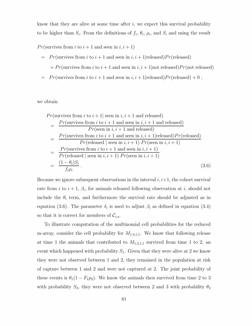
know that they are alive at some time after i, we expect this survival probability
to be higher than Si. From the definitions of fi, θi, ρi, and Si and using the result
Pr(survives from i to i + 1 and seen in i, i+ 1)
= Pr(survives from i to i + 1 and seen in i, i+ 1|released)Pr(released)
+ Pr(survives from i to i + 1 and seen in i, i + 1|not released)Pr(not released)
= Pr(survives from i to i + 1 and seen in i, i+ 1|released)Pr(released) + 0 ,
we obtain
Pr(survives from i to i+ 1| seen in i, i+ 1 and released)
=Pr(survives from i to i+ 1 and seen in i, i+ 1 and released)
Pr(seen in i, i+ 1 and released)
=Pr(survives from i to i+ 1 and seen in i, i+ 1|released)Pr(released)
Pr(released | seen in i, i+ 1) Pr(seen in i, i+ 1)
=Pr(survives from i to i+ 1 and seen in i, i+ 1)
Pr(released | seen in i, i + 1) Pr(seen in i, i+ 1)
=(1 − θi)Si
fiρi
. (3.6)
Because we ignore subsequent observations in the interval i, i+1, the cohort survival
rate from i to i + 1, βi, for animals released following observation at i, should not
include the θi term, and furthermore the survival rate should be adjusted as in
equation (3.6). The parameter δi is used to adjust βi as defined in equation (3.4)
so that it is correct for members of Ci,.
To illustrate computation of the multinomial cell probabilities for the reduced
m-array, consider the cell probability for M1,3,1,1. We know that following release
at time 1 the animals that contributed to M1,3,1,1 survived from time 1 to 2, an
event which happened with probability S1. Given that they were alive at 2 we know
they were not observed between 1 and 2, they remained in the population at risk
of capture between 1 and 2 and were not captured at 2. The joint probability of
these events is θ1(1 − F1p2). We know the animals then survived from time 2 to 3
with probability S2, they were not observed between 2 and 3 with probability θ2
81

and they remained in the population at risk of capture with probability F2. Given
that they were alive at 3, we know they were captured with probability p3. Thus,
π1,3,1,1 = S1θ1(1 − F1p2)S2θ2F2p3
= α2,1β1 .
The cell probability for M1,3,2,2 is computed in an identical manner with the excep-
tion that the survival probability from 1 to 2 is now conditional on the fact that
the animals were observed and released following observation. Hence
π1,3,2,1 =1 − θ1
f1ρ1S1(1 − F1p2)S2θ2F2p3
= α2,11 − θ1
θ1f1ρ1
β1
= δ1α2,1β1 .
3.2.5 The likelihood function under random emigration
Using the peeling and pooling method described by Burnham (1990) we can express
the likelihood in the form L = Pr(Data|MSS)Pr(MSS) where MSS denotes a set
of jointly minimal sufficient statistics. As shown below we can factor the likelihood
to obtain the result that a MSS is the set of Ri,1 (i = 1,..,t), Ri,2 (i=1,...,t-1),
Ci (i=2,..,t), and Oi (i = 1,...,t − 1) which has dimension 4t − 3, with 4t − 3
free parameters in the model. The distribution of this MSS, i.e. Pr(MSS), can be
expressed as the product of independent binomial terms conditional on the releases,
Ni and ni, and the following functions of the MSS:
Ti = Zi + Ci
and
ri = Zi +Ri,1
where
Zi =
0 i = 1
Zi−1 +Ri−1,1 +Ri−1,2 − Ci −Oi−1 i = 2, ..., t(3.7)
82

The set of “residual” terms, Pr(Data|MSS), are conditionally independent multi-
hypergeometric random variables. This set of terms involves the partial column
totals Mi,j,p,k where
Mi,j,p,k =
i∑
h=1
Mh,j,1,1 +i−1∑
h=1
Mh,j,2,1 k = 1
i∑
h=1
Mh,j,1,2 +Mh,j,2,1 k = 2
Derivation of the factorization L = Pr(Data|MSS)Pr(MSS) is based on re-
peated application of the following theorem:
Theorem 3.1 (Multinomial factorization theorem) Let (X1, ..., Xk) be multi-
nomial with parameters N, p1, ..., pk. Then
Pr(X1, ..., Xk) = Pr(X1)Pr(X2, ..., Xk|N −X1)
where
Pr(X1) =
N
X1
pX1
1 (1 − p1)N−X1
and
Pr(X2, ..., Xk|N −X1) =(N −X1)!
k∏
i=2
Xi!
k∏
i=2
(pi
1 − p1
)Xi
Proof From Larsen and Marx (1986) Theorem 9.2.1, the marginal distribution of
Xi is binomial. Now,
Pr(X1, ..., Xk) = Pr(X1)Pr(X2, ..., Xk|X1)
= Pr(X1)Pr(X1, ..., Xk)
Pr(X1)
=N !
X1!(N −X1)!pX1
1 (1 − p1)N−X1
×
N !k∏
i=1
Xi!
k∏
i=1
(pi
1 − p1
)Xi
N !X1!(N−X1)!
pX11 (1 − p1)N−X1
83

=N !
X1!(N −X1)!pX1
1 (1 − p1)N−X1
×(N −X1)!
k∏
i=2
Xi!
k∏
i=2
(pi
1 − p1
)Xi
= Pr(X1)Pr(X2, ..., XK|N −X1)
Now, we can write the likelihood as
Pr(Data) =t∏
i=
Ni!
(Ni − Ri,)!t∏
j=i+
Mi,j,,!t∏
j=i
Mi,j,,!
×t∏
j=i+1
πMi,j,1,1
i,j,1,1
t∏
j=i
πMi,j,1,2
i,j,1,2 (1 − λi,1)Ni−Ri,1
×t−1∏
i=1
ni!
(ni −Ri,2)!t∏
j=i+1
Mi,j,2,1!t∏
j=i+1
Mi,j,2,2!
×t∏
j=i+1
πMi,j,2,1
i,j,2,1
t∏
j=i+1
πMi,j,2,2
i,j,2,2 (1 − λi,2)ni−Ri,2
(3.8)
where
λi,k =
t∑
j=i+1
πi,j,1,1 +t∑
j=i
πi,j,1,2 k = 1
t∑
j=i+1
πi,j,2,1 +t∑
j=i+1
πi,j,2,2 k = 2
We can also write
λi,1 = (αi,1 + αi,2) + (αi+1,1 + αi+1,2)βi + ...+ (αt−1,1 + αt−1,2)βi · · · βt−2
+ αt,2βi · · · βt−1
= (αi,1 + αi,2) + βiλi+1,1 (3.9)
and
λi,2 = δi (λi,1 − αi,2) . (3.10)
84

Factoring out the marginal distributions of Ri,1 and Ri,2 (strictly Ri,1|Ni and
Ri,2|ni) from (3.8) we obtain
Pr(Data) =t∏
i=
Pr(Ri,|Ni)t−∏
i=
Pr(Mi,i+,,, ...,Mi,t,,,Mi,i,,, ...,Mi,t,,|Ri,)
×t−1∏
i=1
Pr(Ri,|ni)Pr(Mi,i+,,, ...,Mi,t,,,Mi,i+,,, ...,Mi,t,,|Ri,) .
Now, the marginal distributions of the Ri,k’s are binomial, conditional on the num-
bers released in each cohort:
Ri,1 | Ni ∼ B(Ni, λi,1)
Ri,2 | ni ∼ B(ni, λi,2) ,
and the distributions of
(Mi,i+1,1,1, ...,Mi,t,1,1,Mi,i+1,1,2, ...,Mi,t,1,2|Ri,1)
and
(Mi,i+1,2,1, ...,Mi,t,2,1,Mi,i+1,2,2, ...,Mi,t,2,2|Ri,2)
are multinomial, conditional on the Ri,k’s, with multinomial cell probabilitiesπi,j,1,k
λi,1
andπi,j,2,k
λi,2respectively. Hence
Pr(Data) =t∏
i=1
Ni
Ri,1
λRi,1
i,1 (1 − λi,1)(Ni−Ri,1)
×t−1∏
i=1
Ri,1
[Mi,j,1,1]t
j=i+1 , [Mi,j,1,2]t
j=i
t∏
j=i+1
(πi,j,1,1
λi,1
)Mi,j,1,1
×t∏
j=i
(πi,j,1,2
λi,1
)Mi,j,1,2
×t−1∏
i=1
ni
Ri,2
λRi,2
i,2 (1 − λi,2)(ni−Ri,2)
×
Ri,2
[Mi,j,2,1]t
j=i+1 [Mi,j,2,2]t
j=i+1
t∏
j=i+1
(πi,j,2,1
λi,2
)Mi,j,2,1
×t∏
j=i+1
(πi,j,2,2
λi,2
)Mi,j,2,2 (3.11)
85

where
x
[yi]b
i=a
is used to denotex!
b∏
i=a
yi!
.
The next step is to factor Pr(M1,2,1,1,...,M1,t,1,1,M1,1,1,2 ,...,M1,t,1,2|R1,1) obtaining
Pr(M,,,, ...,M,t,,,M,,,, ...,M,t,,|R,) =
Pr(M,,,|R,) × Pr(M,,,|R, −M,,,)
×Pr(M,,,, ...,M,t,,,M,,,, ...,M,t,,|R, −M,,, −M,,,)
(3.12)
where
Pr(M,,,|R,) =
R1,1
M1,1,1,2
(α,
λ,
)M,,,(−
α,
λ,
)R,−M,,,
, (3.13)
and
Pr(M,,,|R, −M,,,) = (3.14)R1,1 −M1,1,1,2
M1,2,1,1
(
α1,1
λ1,1 − α1,2
)M1,2,1,1(
1 −α1,1
λ1,1 − α1,2
)R1,1−M1,1,1,2−M1,2,1,1
.(3.15)
(3.16)
The distribution of (M1,3,1,1,...,M1,t,1,1,M1,2,1,2 ,...,M1,t,1,2|R1,1 −M1,1,1,2 −M1,2,1,1) is
multinomial and making use of relationship (3.9) we find the j, k’th cell probability
is given by
π1,j,1,k
λ1,1 − α1,1 − α1,2=
β1π2,j,1,k
β1λ2,1
=π2,j,1,k
λ2,1.
Similarly, we factor Pr(M1,2,2,1,...,M1,t,2,1, M1,2,2,2,...,M1,t,2,2|R1,2) obtaining
Pr(M,,,, ...,M,t,,,M,,,, ...,M,t,,|R,) =
Pr(M,,,|R,)Pr(M,,,, ...,M,t,,,M,,,, ...,M,t,,|R, −M,,,) .
(3.17)
86

Using the relationship (3.10), we find
Pr(M,,,|R,) =
R1,2
M1,2,2,1
(
α,
λ, − α,
)M,,,(−
α,
λ, − α,
)R,−M,,,
,
(3.18)
and the binomial success parameter α1,1
λ1,1−α1,2is the same as in (3.14). Thus, we can
“pool” (M1,2,1,1|R1,2 −M1,1,1,2 with (M1,2,2,1|R1,2). Noting that M1,2,1,1 +M1,2,2,1 =
C1, M1,1,1,2 = O1, and R1,1 −O1 +R1,2 = T2 we obtain the result
Pr(M1,2,1,1|R1,1 −M1,1,1,2)Pr(M1,2,2,1|R1,2) =R1,1 −M1,1,1,2
M1,2,1,1
R1,2
M1,2,2,1
T2
C2
×
T2
C2
(
α1,1
λ1 − α1,2)C2(1 −
α1,1
λ1 − α1,2)T2−Z2 .
Now, using the relationship (3.9) and (3.10) we find that the j, k’th cell probability
for the conditional multinomial (M1,3,2,1,...,M1,t,2,1,M1,2,2,2 ,...,M1,t,2,2|R1,2−M1,2,2,1)
is given by
π2,j,1,k
λ2,1
.
But,π2,j,1,k
λ2,1is also the j, kth cell probability for the conditional multinomials
(M1,3,1,1, ...,M1,t,1,1,M1,2,1,2, ...,M1,t,1,2|R1,1 −M1,1,1,2 −M1,2,1,1)
and
(M2,3,1,1, ...,M2,t,1,1,M2,2,1,2, ...,M2,t,1,2|R2,1)
thus we are able to “pool” the corresponding cell counts. Now,
M1,j,1,k +M1,2,2,k +M2,j,1,k = M2,j,p,k
and
R1,1 −M1,1,1,2 − C1 +R1,2 +R2,1 = r2
87

hence the result
Pr(M,,,, ...,M,t,,,M,,,, ...,M,t,,|R, −M,,, −M,,,)
×Pr(M,,,, ...,M,t,,,M,,,, ...,M,t,,|R, −M,,,)
×M2,3,1,1, ...,M2,t,1,1,M2,3,1,2, ...,M2,t,1,2|R2,1)
=
R1,1 −M1,1,1,2 −M1,2,1,1
[M1,j,1,1]t
j=3 , [M1,j,1,2]t
j=2
R1,2 −M1,2,2,1
[M2,j,2,1]t
j=3 , [M2,j,2,2]t
j=2
r2
[M2,j,p,1]t
j=3 , [M2,j,p,2]t
j=2
×
R2,1
[M2,j,1,1]t
j=3 , [M2,j,1,2]t
j=2
× Pr(M2,3,p,1, ...,M2,t,p,1,M2,2,p,2, ...,M2,t,p,2|r2) ,
where
Pr(M2,3,p,1, ...,M2,t,p,1,M2,2,p,2, ...,M2,t,p,2|r2) =
r2
[M2,j,p,1]t
j=3 , [M2,j,p,2]t
j=2
t∏
j=3
π2,j,1,1
λ2,1
t∏
j=2
π2,j,1,2
λ2,1.
To complete the derivation of Pr(MSS) we make repeated use of the following
factorizations:
Pr(Mi,i+,p,, ...,Mi,t,p,,Mi,i,p,, ...,Mi,t,p,|ri) =
Pr(Mi,i,p,|ri) × Pr(Mi,i+,p,|ri −Mi,i,p,)
×Pr(Mi,i+,p,, ...,Mi,t,p,,Mi,i+,p,, ...,Mi,t,p,|ri −Mi,i,p, −Mi,i+,p,) ,
and
Pr(Mi,i+,,, ...,Mi,t,,,Mi,i+,,, ...,Mi,t,,|Ri,) =
Pr(Mi,i+,,|Ri,)Pr(Mi,i+,,, ...,Mi,t,,,Mi,i+,,, ...,Mi,t,,|Ri, −Mi,i+,,)
where
Pr(Mi,i,p,|ri) = Pr(Oi|ri)
=
ri
Oi
(αi,2
λi,1
)Oi(
1 −αi,2
λi,1
)ri−Oi
, (3.19)
88

Pr(Mi,i+,,|ri − Oi) =
ri − Oi
Mi,i+1,p,1
(
αi,1
λi,1 − αi,2
)Mi,i+1,p,1(
1 −αi,1
λi,1 − αi,2
)ri−Oi−Mi,i+1,p,1
(3.20)
Pr(Mi,i+1,2,1|Ri,2) =
Ri,2
Mi,i+1,2,1
(
αi,1
λi − αi,2
)Mi,i+1,2,1(
1 −αi,1
λi − αi,2
)Ri,2−Mi,i+1,2,1
, (3.21)
(Mi,i+2,1,1,...,Mi,t,1,1,Mi,i+1,1,2 ,...,Mi,t,1,2|Ri,1−Mi,i,1,2−Mi,i+1,1,1) is multinomial with
i, j, k’th cell probability given by
πi,j,1,k
λi,1 − αi,1 − αi,2=
πi+1,j,1,k
λi+1,1
and (Mi,i+2,2,1,...,Mi,t,2,1,Mi,i+1,2,2 ,...,Mi,t,2,2|Ri,2 − Mi,i+1,2,1) is multinomial with
i, j, k’th cell probability also given by
πi+1,j,1,k
λi+1,1
.
Now, (Mi,i+1,p,1|ri−Oi) and (Mi,i+1,2,1|Ri,2) have the same binomial success param-
eter so can be “pooled” forming (Ci+1|Ti+1) because ri−Oi+Ri,2 = Ti+1. Similarly,
the multinomial cell probabilities for (Mi,i+2,1,1, ...,Mi,t,1,1,Mi,i+1,1,2, ...,Mi,t,1,2|ri −
Oi−Mi,i+1,1,1) and (Mi,i+2,2,1, ...,Mi,t,2,1,Mi,i+1,2,2, ...,Mi,t,2,2|Ri,2−Mi,i+2,2,1) are the
same as the cell probabilities for the conditional multinomial
(Mi+1,i+2,1,1, ...,Mi+1,t,1,1,Mi+1,i+1,1,2, ...,Mi+1,t,1,2|Ri+1,1)
hence corresponding cell counts can be pooled to form
(Mi+1,i+2,p,1, ...,Mi+1,t,p,1,Mi+1,i+1,p,2, ...,Mi+1,t,p,2|ri+1) ,
since
Mi+1,t,p,k = Mi,t,p,k +Mi,t,2,k +Mi+1,t,1,k
and making use of (3.7)
ri+1 = ri − Oi − Ci+1 +Ri,2 +Ri+1,1
= Zi +Ri,1 −Oi − Ci+1 +Ri,2 +Ri+1,1
= Zi+1 +Ri+1,1
89

Noting that r1 = R1,1, O1 = M1,1,1,2, and M1,j,p,k = M1,j,1,k we begin with cohort 1,
and iterate the “peeling” and “pooling” (factorization) cycles up to and including
cohorts Ct−, and Ct−,, and then Ct,. At each cycle we
1. “peel” off a
Pr(Mi,i,p,2|ri) =
ri
Oi
(αi,2
λi,1
)Oi(
1 −αi,2
λi,1
)ri−Oi
,
term,
2. “peel” then “pool” to form a
Pr(Mi,i+,,|ri −Oi) × Pr(Mi,i+,,|Ri,) =
ri −Oi
Mi,i+1,1,1
Ri,2
Mi,i+1,2,1
Ti+1
Ci+1
×
Ti+1
Ci+1
(
αi,1
λi − αi,2)Ci+1(1 −
αi,1
λ1 − αi,2)Ti+1−Zi+1 .
term
3. then “pool” the residual terms to form a
Pr(Mi,i+,,, ...,Mi,t,,,Mi,i+,,, ...,Mi,t,,|ri − Oi −Mi,i+,,)
×Pr(Mi,i+,,, ...,Mi,t,,,Mi,i+,,, ...,Mi,t,,|R, −M,,,)
×Mi+1,i+2,1,1, ...,Mi+1,t,1,1,Mi+1,i+2,1,2, ...,Mi+1,t,1,2|R2,1
=
ri − Oi −Mi,i+1,1,1
[Mi,j,1,1]t
j=i+2 , [Mi,j,1,2]t
j=i+1
Ri,2 −Mi,i+1,2,1
[Mi+1,j,2,1]t
j=i+2 , [Mi+1,j,2,2]t
j=i+1
ri+1
[Mi+1,j,p,1]t
j=i+2 , [Mi+1,j,p,2]t
j=i+1
×
Ri+1,1
[Mi+1,j,1,1]t
j=i+2 , [Mi+1,j,1,2]t
j=i+1
90

×
ri+1
[Mi+1,j,p,1]t
j=i+2 , [Mi+1,j,p,2]t
j=i+1
t∏
j=i+2
πi+1,j,1,1
λi+1,1
t∏
j=i+1
πi+1,j,1,2
λi+1,1
(3.22)
term.
After cycle t, the residual term given by (3.22) has the value 1 hence Pr(Data)
= L reduces to
L =t∏
i=1
Ni
Ri,1
(λi,1)
Ri,1 (1 − λi,1)(Ni−Ri,1)
t−1∏
i=1
ni
Ri,2
(λi,2)
Ri,2 (1 − λi,2)(ni−Ri,2)
×t∏
i=2
Ti
Ci
(τi,1)
Ci (1 − τi,1)Zi
t−1∏
i=1
ri
Oi
(τi,2)
Oi (1 − τi,2)ri−Oi
×t∏
i=2
ri−1 − Oi−1
Ci −Mi−1,i,2,1
Ri−1,2
Mi−1,1,2,1
Ti
Ci
×
t−2∏
i=1
ri − Oi −Mi,i+1,p,1
[Mi,j,p,1]t
j=i+2 [Mi,j,p,2]t
j=i+1
Ri+1(1)
[Mi+1,j,1,1]t
j=i+2 [Mi+1,j,1,2]t
j=i+1
ri+1
[Mi+1,j,p,1]t
j=i+2 [Mi+1,j,p,2]t
j=i+1
×
Ri,2 −Mi,i+1,2,1
[Mi,j,2,1]t
j=i+2 [Mi,j,2,2]t
j=i+1
1
, (3.23)
91

where
τi+1,1 =αi,1
λi,1 − αi,2i = 2, ..., t
and
τi,2 =αi,2
λi,1i = 1, ..., t− 1
Thus, we have the result that the distribution of the MSS Ri,1 (i = 1,..,t), Ri,2, Ci
(i=2,..,t, and Oi (i = 1,...,t−1) can be expressed as the product of the conditionally
independent binomial random variables:
Ri,1 | Ni ∼ B(Ni, λi,1) i = 1, ..., t
Ri,2 | ni ∼ B(ni, λi,2) i = 1, ..., t− 1
Ci | Ti ∼ B(Ti, τi,1) i = 2, ..., t
Oi | ri ∼ B(ri, τi,2) i = 1, ..., t− 1 .
The remaining “residual” term in the distribution of the data (i.e. Pr(data|MSS))
is the product of conditionally independent hypergeometric distributions. To see
that these residual terms are of the form of multi-hypergeometric random variables,
note that each component takes the form
I∏
i=1
ai
bi,1, ..., bi,J
a.
b.,1, ..., b.,J
(3.24)
where a. =I∑
i=1
ai and b., j =I∑
i=1
bi,j. The ai partition the sufficient statistic a., and
the mutually exclusive set bi,1, ..., bi,k, conditional on ai, are multinomial random
variables with cell probabilities π1,...,πk. Recall that these terms result from the
pooling of observations that had the same conditional cell-probabilities hence these
cell probabilities are common for all i. We will return to these when we consider
goodness-of-fit tests for this model.
92

3.2.6 Parameter estimation
The parameters of interest Si, θi, fi, and the confounded pair Fipi+1 = p∗i+1 are
one-to-one functions of the λi,1, λi,2, τi,1, and τi,2:
fi =
τi,2λi,1 i = 1, ..., t− 1
λt,1 i = t
p∗i =λi,1τi,1
1 + (λi,1 − 1)τi,1)
θi =1 − τi,2
1 + τi,2(λi,2 − 1)
and
Si = (1 + τi,2(λi,2 − 1))λi,1
λi+1,1
{1 + τi+1,1(λi,1 − 1)} .
Note also, that δi is only defined with respect to marked animals. Since we condition
on the releases, the probability ρi which appears in δi is taken to be exactly ni/Oi,
and is known without error (i.e. for all marked animals resighted in (i, i + 1) we
know whether or not they were released).
Substituting the MLE’s
λi,1 =Ri,1
Ni
λi,2 =Ri,2
ni
τi,1 =Ci
Ti
and
τi,2 =Oi
ri
and solving for fi, p∗
i ,θi, and Si, leads to the MLE’s
fi =
Ri,1
Nii = t
OiRi,1
Nirii = 1, ..., t− 1
(3.25)
p∗i =Ci
NiZi
Ri,1+ Ci
i = 2, ..., t (3.26)
93

θi =ri −Oi
Ti+1i = 1, ..., t− 1 (3.27)
and
Si =Ri,1
Niri
{Ni+1Zi+1
Ri+1,1+ Ci+1
}i = 1, ..., t− 1 . (3.28)
Note that p∗i and Si are the Jolly-Seber estimators but with Ri,1 and Zi augmented
by the inclusion of observed animals.
For example, from Table 3.6 we obtain
f1 = O1R1,1
N1r1
= 108×2641000×264
= 0.1080
p∗2 = C2N2Z2R2,1
+C2
= 631000×123
237+63
= 0.1082
θ1 = n1(r1−O1)r1n1+O1(R1,2−n1)
= 108×(264−108)264×108+108×(30−108)
= 0.8387
and
S1 = R1,1
N1r1
{N2Z2
R2,1+ C2
}
= 2641000×264
(1000×123
237+ 63
)
= 0.5820
Estimates of the remaining parameters and their standard errors (see following
section) are given in Table 3.9
94

Table 3.9: Parameter estimates and associated standard errors for the hypothetical
mark-recapture data.
Year p∗i se(p∗i ) θi se(θi) fi se(fi) Si se(Si)
1 .8387 .0270 .1080 .0098 .5820 .0527
2 .1082 .0159 .8571 .0224 .0988 .0083 .5852 .0550
3 .0911 .0124 .8990 .0214 .1045 .0084 .5758 .0735
4 .0932 .0143 .1070 .0098
3.2.7 Asymptotic variances and covariances
Using the delta-method (Seber 1982) asymptotic variances and covariances can be
readily obtained. We make use of the following partial derivatives (all other partial
derivatives are zero):
∂fi
∂λi,1=
fi
λi,1(i = 1, ..., t− 1)
1 i = t
∂fi
∂τi,2=
fi
τi,2(i = 1, ..., t− 1)
0 i = t
∂Si
∂λi,1
=Si
λi,1
,
∂Si
∂λi+1,1=
−Si(1 − p∗i+1)
λi+1,1
∂Si
∂λi,2=Si(1 − θi)
λi,2
∂Si
∂τi+1,1=
−Sip∗
i+1(1 − λi+1,1)
τi+1,1λi+1,1
∂Si
∂τi,2=Siθi(λi,2 − 1)
1 − τi,2
∂θi
∂λi,2=
−θi(1 − θi)
λi,2
∂θi
∂τi,2=
−θi(1 − θi)
τi,2(1 − τi,2)
∂p∗i∂λi,1
=p∗i (1 − p∗i )
λi,1
95

∂p∗i∂τi,1
=p∗i (1 − p∗i )
τi,1(1 − τi,1)
Following Pollock et al. (1990) we use the notation V ar(fi) to denote V ar(fi|fi),
and similarly for the other parameters. The variances and non-zero covariances are
obtained as follows:
For i = 1, ..., t− 1
V ar(fi) =
(∂fi
∂λi,1
)2
V ar(λi,1|Ni) +
(∂fi
∂τi,2
)2
V ar(τi,2|ri)
= f 2i
(1 − λi,1
λi,1Ni
+1 − τi,2τi,2ri
)
= f 2i
(1
E[Ri,1]−
1
Ni
+1
E[Oi]−
1
ri
)
V ar(ft) = V ar(λt,1|Nt)
=E [Rt,1] (Nt − E [Rt,1])
N3t
= f 2t
(1
E[Rt,1]−
1
Nt
)
V ar(Si) =
(∂Si
∂λi,1
)2
V ar(λi,1|Ni) +
(∂Si
∂λi+1,1
)2
V ar(λi+1,1|Ni+1) +
(∂Si
∂λi,2
)2
×V ar(λi,2|ni) +
(∂Si
∂τi+1,1
)2
V ar(τi+1,1|Ti+1)
+
(∂Si
∂τi,2
)2
V ar(τi,2|ri)
= S2i
{1
E[Ri,1]−
1
Ni
+ (1 − p∗i+1)2
(1
E[Ri+1,1]−
1
Ni+1
)
+ p∗i+1(1 − p∗i+1)(Ni+1 −Ri+1,1)
2
Ni+1Ri+1,1Ti+1+ (1 − θi)
2
(1
E[Ri,2]−
1
ni
)
+
[θi (Oi − E[Ri,2])
ni
]2 (1
ri − E[Oi]−
1
ri
)
V ar(θi) =
(∂θi
∂λi,2
)2
V ar(λi,2|ni) +
(∂θi
∂τi,2
)2
V ar(τi,2|ni)
= θ2i (1 − θi)
2
(1
τi,2(1 − τi,2)ri
+1 − λi,2
λi,2ni
)
= [θi(1 − θi)]2
(1
E[Oi]+
1
(ri − E[Oi])+
1
E[Ri,2]−
1
ni
)
96

V ar(p∗i ) =
(∂p∗i∂λi,1
)2
V ar(λi,1|Ni) +
(∂p∗i∂τi,1
)2
V ar(τi,1|Ti)
=
[p∗i (1 − p∗i )
λi,1
]2λi,1(1 − λi,1)
Ni
+ [pi ∗ (1 − p∗i )]2 1
τi,1(1 − τi,1)Ti
= [p∗i (1 − p∗i )]2
(1
Ri,1−
1
Ni
+1
Ci
+1
Zi
)
Cov(fi, Si) =
(∂fi
∂λi,1
)(∂Si
∂λi,1
)V ar(λi,1|Ni) +
(∂fi
∂τi,2
)(∂Si
∂τi,2
)V ar(τi,2|ri)
= fiSi
(1 − λi,1
λi,1Ni
+fiSiθi(λi,2 − 1)
ri
)
= fiSi
(1
E[Ri,1]−
1
Ni
+θi(E[Ri,2] − ni)
niri
)
Cov(fi, p∗
i ) =
(∂fi
∂λi,1
)(∂p∗i∂λi,1
)V ar(λi,1|Ni)
= fip∗
i (1 − p∗i )
(1 − λi,1
λi,1Ni
)
= fip∗
i (1 − p∗i )
(1
E[Ri,1]−
1
Ni
)
Cov(fi+1, Si) =
(∂fi+1
∂λi+1,1
)(∂Si
∂λi+1,1
)V ar(λi+1,1|Ni+1)
= −fi+1Si(1 − p∗i+1)
(1 − λi+1,1
λi+1,1Ni+1
)
= −fi+1Si(1 − p∗i+1)
(1
E[Ri+1,1]−
1
Ni+1
)
Cov(Si, Si+1) =
(∂Si
∂λi+1,1
)(∂Si+1
∂λi+1,1
)V ar(λi+1,1|Ni+1)
= −SiSi+1(1 − p∗i+1)
(1 − λi+1,1
λi+1,1Ni+1
)
= −SiSi+1(1 − p∗i+1)
(1
E[Ri+1,1]−
1
Ni+1
)
Cov(Si, θi) =
(∂Si
∂λi,2
)(∂θi
∂λi,2
)V ar(λi,2|ni) +
(∂Si
∂τi,2
)(∂θi
∂τi,2
)V ar(τi,2|ri)
97

= −Siθi(1 − θi)
((1 − θi)(1 − λi,2)
λi,2ni
+θi(λi,2 − 1)
(1 − τi,2)ri
)
= −Siθi(1 − θi)2
(1
E[Ri,2]−
1
ni
+θi
(1 − θi)Oi
(E[Ri,2] − Oi)
ri − E[Oi]
)
Cov(Si, pi+1) =
(∂Si
∂λi+1,1
)(∂pi+1
∂λi+1,1
)V ar(λi+1,1|Ni+1) +
(∂Si
∂τi+1,1
)(∂pi+1
∂τi+1,1
)
×V ar(τi+1,1|Ti+1)
= −Si(1 − p∗i+1)2p∗i+1
(1 − λi+1,1
λi+1,1Ni+1
)− Si[p
∗
i+1]2(1 − p∗i+1)
×
(1 − λi+1,1
λi+1,1τi+1,1Ti+1
)
= −Si(1 − p∗i+1)2p∗i+1
(1
E[Ri+1,1]−
1
Ni+1+
p∗i+1
1 − p∗i+1
×Ni+1 − E[Ri+1,1]
E[Ri+1,1]E[Ci+1]
)
Cov(Si, pi) =
(∂Si
∂λi,1
)(∂pi
∂λi,1
)V ar(λi,1|Ni)
= Sip∗
i (1 − p∗i )
(1 − λi,1
λi,1Ni
)
= Sipi(1 − p∗i )
(1
E[Ri,1]−
1
Ni
)
In the above expressions all the expectations are with respect to the appropriate
binomial indices. Estimates of the above variances and covariances can be obtained
by substituting observed values for expected values and parameter estimates for the
parameters.
Replacing parameters by their estimates and expected values by observed values,
we obtain for our hypothetical example (Table 3.6),
V ar(p∗2) = [p∗2(1 − p∗i )]2
(1
Ri,1−
1
Ni
+1
Ci
+1
Zi
)
= [0.1082 × 0.8918]2(
1
237−
1
1000+
1
63+
1
123
)
= 0.0002535
98

V ar(θ1) =[θ1(1 − θ1)
]2(
r1O1(r1 − O1)
+1
R1,2−
1
n1
)
= [0.8387 × 0.1613]2(
264
108 × (264 − 108)+
1
30−
1
108
)
= 0.0007274 (3.29)
V ar(f1) = f 21
(1
R1,1−
1
N1+
1
O1−
1
r1
)
= 0.10802(
1
264−
1
1000+
1
108−
1
264
)
= 0.0000963 (3.30)
and
V ar(S1) = S21
{1
R1,1−
1
N1+ (1 − p∗2)
2
(1
R2,1−
1
N2
)
+ p∗2(1 − p∗2)(N2 − R2,1)
2
N2R2,1T2+ (1 − θ1)
2
(1
R1,2−
1
n1
)
+θ21 (n1 −R1,2)
n1
(1
r1 − E[O1]−
1
r1
)}
= 0.5820{
1
264−
1
1000+ 0.89182
(1
237−
1
1000
)
+ 0.1082 × 0.8918(1000 − 237)2
1000 × 237 × 186+ 0.16132
(1
30−
1
108
)
+0.83872 (108 − 30)
108
(1
264 − 108−
1
264
)}
= 0.0028
Standard errors (se(p∗i ) =√V ar(p∗i ) etc) for the remaining parameter estimates
are given in Table 3.9.
3.2.8 Goodness-of-fit tests under random emigration
From (3.23) we obtained the result that the distribution of the MSS could be
factored into a component depending on the parameters and a “residual” com-
ponent which takes the form of independent multi-hypergeometric distributions
conditional on sufficient statistics. Following Pollock et al. (1985) (see also Rob-
son 1969, Brownie and Robson 1983) we can utilize this component to develop
goodness-of-fit tests.
99

We exploit the fact that in each multi-hypergeometric term the bi,j, (j=1,...,J)
of expression (3.24) are multinomial with cell probabilities in common for all i. This
allows us to form an I × J contingency table corresponding to each component of
the residual distribution.
From (3.23) the residual component comprises two parts:
t∏
i=2
ri−1 − Oi−1
Ci −Mi−1,i,2,1
Ri−1,2
Mi−1,i,2,1
Ti
Ci
(3.31)
and
t−2∏
i=1
ri − Oi −Mi,i+1,p,1
[Mi,j,p,1]t
j=i+2 [Mi,j,p,2]t
j=i+1
Ri+1,1
[Mi+1,j,1,1]t
j=i+2 [Mi+1,j,1,2]t
j=i+1
ri+1
[Mi+1,j,p,1]t
j=i+2 [Mi+1,j,p,2]t
j=i+1
×
Ri,2 −Mi,i+1,2,1
[Mi,j,2,1]t
j=i+2 [Mi,j,2,2]t
j=i+1
1(3.32)
In the first component (3.31), the sufficient statistic Ti, the total number of
marked animals at i that are captured or seen at i, or at any time after i, is
partitioned into ri−1−Oi−1 and Ri−1,2. This provides a partitioning of Ti according
to whether the animals were observed at i − 1 or not. The term Ci − Mi−1,i,2,1
represents those members of Ti not observed at i − 1 that were captured at i,
and the term Mi−1,1,2,1 represents those members of Ti observed at i− 1 that were
captured at i. Thus from this component we can form (t−1) 2×2 contingency tables
which test whether the event “member of Ti and captured at i” is independent of
the event “member of Ti and observed at i− 1”. Thus the component (3.31) leads
to a test of whether observation has a short-term (i.e. one sampling period) effect
on the probability that the animal is captured. Note that this effect may occur
through influences on any of the pi, Si−1, or Fi−1. This test may be particularly
100

important in a study where “observation” involves physically handling the animals.
The general form of these contingency tables is illustrated in Table 3.10.
Table 3.10: Example of a 2×2 contingency table for the component 1 goodness-of-fit
test
Member of Ti Member of Ti
captured at i not captured at i
Observed at i− 1 Mi−1,i,2,1 Ri−1,2 −Mi−1,i,2,1 Ri−1,2
Not observed at i− 1 Ci −Mi−1,i,2,1 ri−1 − Oi−1 − Ci +Mi−1,i,2,1 ri−1 − Oi−1
Ci Zi Ti
To illustrate using a numerical example we partition T2 from the data in Table
3.5 giving
r1 − O1 = 264 − 108 = 156
R1,2 = 30
C2 −M1,2,2,1 = 63 − 12 = 51
M1,2,2,1 = 12
and hence the contingency table
Member of T2 Member of T2
captured at 2 not captured at 2
Observed at 1 12 18 30
Not observed at 1 51 105 156
63 123 186
The null hypothesis of independence of the events “ observed at time 1” and
“captured at time 2” for members of T2 cannot be rejected χ21 = 0.60, p = 0.44,
so there is no evidence of a one-period effect of observation on the probability of
capture at time 2.
101

In the component (3.32) the sufficient statistic ri+1 is partitioned into ri −Oi −
Mi,i+1,p,1, Ri+1,1, and Ri,2 −Mi,i+1,2,1. These represent a partitioning of ri+1 firstly
according to whether the animals were captured at i + 1, and secondly for those
animals not captured at i+ 1, according to whether they were observed at i. Note,
if a member of ri+1 was not captured at i we know that it was marked at or before
i. The second partitioning of ri+1 is by release/observation category. Thus, from
component (3.32) we form (t − 3) 2(t − i − 1) × 3 contingency tables, which test
whether membership in one of the capture/observation cells Mi,i+2,p,1, ...,Mi,t,p,1,
Mi,i+1,p,2, ...,Mi,t,p,2 is independent of the events “captured at i+1”, “not captured
at i + 1 and not observed at i”, and “not captured at i + 1 and observed at i”.
Therefore this test will be sensitive to a “capture” effect (short- or long-term) on
the probability that the animal is captured or seen again and an “observation”
effect (short- or long-term) on the probability the animal is captured or seen again.
A particularly important “capture” effect occurs when the random emigration as-
sumption is violated (see section 3.6), therefore this component tests, among other
things, the random emigration assumption. An example showing the general form
of a component 2 contingency table is provided in Table 3.11.
A numerical example using the data from Table 3.5 gives the partitioning of r2
R1,1 −O1 −M1,2,p,1 = 264 − 108 − 51 = 105
R1,2 −M1,2,2,1 = 30 − 12 = 18
R2,1 = 237
with the corresponding contingency table
102

Table 3.11: Example of a contingency table for the component 2 goodness-of-fit
test at time i.
Member of ri+1 Member of ri+1 Member of ri+1
not observed at i observed at i captured at i + 1
not captured not captured
at i+ 1 at i+ 1
Member of Mi,i+2,p,1 Mi,i+2,2,1 Mi+1,i+2,1,1 Mi+1,i+2,p,1
Mi+1,i+2,p,1
. . . .
. . . .
. . . .
Member of Mi,t,p,1 Mi,t,2,1 Mi+1,t,1,1 Mi+1,i+2,p,1
Mi+1,t,p,1
Member of Mi,i+1,p,2 Mi,i+1,2,2 Mi+1,i+1,1,2 Mi+1,i+1,p,2
Mi+1,i+1,p,2
. . . .
. . . .
. . . .
Member of Mi,t,p,2 Mi,t,2,2 Mi+1,t,1,2 Mi+1,i+2,p,2
Mi+1,t,p,2
Ri,1 −Oi −Mi,i+1,p,1 Ri,2 −Mi,i+1,2,1 Ri+1,1 ri+1
103

Member of r2 Member of r2 Member of r2
not observed at 1 observed at 1 captured at 1
not captured at 2 not captured at 2
Member of M2,3,p,1 16 2 50 68
Member of M2,4,p,1 13 3 19 35
Member of M2,2,p,2 48 8 94 150
Member of M2,3,p,2 16 4 56 76
Member of M2,4,p,2 12 1 18 31
105 18 237 360
Because several of the cells have expected values less than 5, and one has an ex-
pected value less than 2, the chi-squared approximation may not be good. This
is likely to be a commonly encountered problem. Under these circumstances two
approaches may be used. The first is to compute the probability of the observed,
or a more extreme, result exactly using the hypergeometric distribution. In most
cases this approach is likely to be computationally intensive, although there are
algorithms for r× c tables (Mehta and Patel 1983). The alternative approach is to
pool cells, and use the large sample chi-square approximation on the pooled data.
Because in the multi-hypergeometric term we are conditioning on the marginal
totals Ri,1 −Oi −Mi,i+1,p,1, Ri,2 −Mi,i+1,2,1, and Ri+1,1 an obvious pooling rule is to
maintain these marginal values and instead pool the elements Mi,j,p,k across some j.
Alternatively, or in addition, we can pool columns of the contingency table e.g. data
for members of Ri,1 − Oi −Mi,i+1,p,1 with data for members of Ri,2 −Mi,i+1,2,1(see
section 3.6). A pooled contingency table from the above example, with pooling
across some j
104

Member of r2 Member of r2 Member of r2
not observed observed at 1 captured at 2
at 1, not not captured
captured at 2 at 2
Captured at 29 5 69 103
or after 3
Not captured, 48 8 94 150
observed at 2
Not captured, 28 5 74 107
observed after 2
105 18 237 360
and provides no evidence that the probability an animal was captured at time 3 or
later was influenced by whether it was captured at 2 or observed at 1 (χ42 = 1.27,
p = 0.867).
Even in the “exact” hypergeometric case, it may still be preferable to pool if
several of the cell expected values are small. The power of the hypothesis tests
under pooling will tend to be more powerful than in the unpooled case. However,
it is important to note that pooling changes the hypothesis being tested.
3.3 Permanent emigration
In the permanent emigration model we allow animals to leave the at risk of capture
component of the population between i and i + 1, but these animals can never
return. As in the random emigration model the probability an animal at risk of
capture at i and alive at i+ 1 is at risk of capture at i+ 1 is given by Fi. However,
in the permanent emigration model the probability an animal not at risk of capture
at i and alive at i+ 1 is at risk of capture at i+ 1 is zero.
Because emigration is permanent, the probability an animal released at i and
alive at j, is at risk of capture at j but was not captured between i and j is given
105

by
γi,j,1 = Fj−1
j−2∏
h=i
Fh(1 − ph+1) . (3.33)
i.e. because emigration is permanent, such an animal must be at risk of capture at
each of i, i+1, .., j. In contrast, all animals are at risk of being observed, regardless
of whether or not they are at risk of capture. For animals released at i there are
j − i+ 1 possible pathways by which they can be not recaptured between i and j,
complicating computation of γi,j,2. This can be computed recursively as follows:
Let ai,j denote the probability an animal alive and at risk of capture at i, and
alive at j, is at risk of capture at j, but is not captured between i and j. Similarly,
let bi,j denote the probability an animal alive and at risk of capture at i, and alive
at j, is not at risk of capture at j and is not captured between i and j. Then
ai,j =
Fj−1 j = i+ 1
ai,j−1(1 − pj−1)Fj−1 j = i+ 2, ..., t(3.34)
and
bi,j =
(1 − Fj−1) j = i+ 1
ai,j−1(1 − pj−1)(1 − Fj−1) + bi,j−1 j = i+ 2, ..., t, (3.35)
then
γi,j,2 = ai,j(1 − pj) + bi,j (3.36)
Utilizing (3.33) the probability structure for the model under permanent emigration
for animals last released following capture is given as follows. Let
αi,1 = SiFiθipi+1
αi,2 = fi
and
βi = Siθi .
106

then
πi,j,1,k =
αi,1 (j = i+ 1, k = 1)
αi,2 (j = i, k = 2)
αj−1,1γi,j,1
j−2∏
h=i
βh (j = i+ 2, ..., t, k = 1)
αj,2γi,j,2
j−1∏
h=i
βh (j = i+ 1, ..., t, k = 2)
. (3.37)
For animals released following observation, the situation is more complicated, as
the subscript i in γi,j,k indexes the last capture occasion. The consequence is that
the m-array data summary used under random emigration is not sufficient under
permanent emigration. One remedy is to partition the ni and the Mi,j,2,k’s according
to last capture occasion. The second is to model the capture histories directly.
Let h denote a specific capture history. Derivation of Pr(h) involves partitioning
Pr(h|first release) into three parts (K.P. Burnham pers. comm):
Pr(last encounter|first release)×
Pr(encounter history between first and last encounter|first release and last encounter)
× Pr(never encountered again after last encounter|last encounter) .
For an animal first released at i and last encountered at j, the first term is
Pr(last encounter|first release) =
Si · · · Sj−1fj if last encounterd by observation
Si · · · Sj−1pj if last encounterd by capture.
The encounter history between the first and last encounters can be broken into two
parts, one part for the recaptures and one part for the resightings. The component
for the recaptures will involve the product of Fhph+1 and Fh(1 − ph+1) terms (h ≤
t − 1), and for an animal which was last recaptured and released at k but not
captured at j (k < j), there will be an additional γk,j,2 term. The component for
resightings will simply involve the product of θh and (1 − θh) terms.
For example, for the fictitious animal with capture history h = 05013 discussed
in section 3.2.3 the information we have available is:
(i) The animal was captured at time 2, released, and resighted between 2
and 3 and released.
107

(ii) The animal was captured and released at time 4, but not resighted
between times 4 and 5.
(iii) The animal was resighted between times 5 and 6 and was released on
resighting.
Note that because the animal was recaptured at time 4 we know it must have been
at risk of capture at time 3 even though it was not captured. However, because all
encounters after time 4 were resightings we do not know whether it was at risk of
capture at time 5.
From the above information
Pr(last encounter|first release) = S2S3S4f5 .
To compute
Pr(encounter history between first and last encounter|first release and last encounter)
we note that following release at time 2, and before the last encounter by resighting
between times 5 and 6, the animal was recaptured at time 4, and resighted between
times 2 and 3. Therefore, the recapture at time 4 will contribute an F2(1− p3)F3p4
term, and the resightings a (1 − θ2)θ3θ4 term. Also, the last recapture was at time
4 and it was resighted between times 5 and 6, therefore we will need a γ4,5,2 term,
leading to
Pr(encounter history between first and last encounter|first release and last encounter)
= F2(1 − p3)F3p4(1 − θ2)θ3θ4γ4,5,2 .
In this example, computation is simplified because the animal was observed during
interval 5 = t, and
Pr(never encountered again after last encounter|last encounter) = 1 ,
hence
Pr(h = 05013|first release at 2) =
F2S2(1 − θ2)(1 − p3)S3θ3F3p4S4θ4f5 ∗ {F4(1 − p5) + (1 − F4)}
= p2F2S2(1 − θ2)(1 − p3)S3θ3F3p4S4θ4f5γ4,5,2 .
108

If capture and observation are possible for periods following the last occasion on
which the animal was captured or observed, an additional term for the probability
that an animal last encountered at j is never encountered again must be computed.
This term is most easily obtained as 1−Pr(animal is encountered again|last release at j)
and is obtained by partitioning the compound event
(animal is encountered again|last release at j)
into the set of disjoint events
(animal is encountered at h|last release at j)
for each h > j (K.P. Burnham, pers. comm.).
Once Pr(h|first release) is determined for each animal the likelihood function is
then
L =∏
h
{Pr(h|first release)}Xh
where Xh is the number of animals sharing capture history h.
Because the observation component of the model is expressed in terms of the
γi,j,2’s the likelihood does not factor as in (3.23) and closed-form maximum like-
lihood estimates do not appear to exist (see comments by Burnham 1993). Thus
numerical procedures must be used to compute the maximum-likelihood estimates.
Because emigration is permanent the pathways involved in γi,t,2 are one of three
possible types: one pathway where animals were at risk of capture at t, but not
captured, another where the animals were at risk of capture at t− 1 but not at t,
and a remaining set where the animals left the at risk of capture component of the
population before t− 1. Thus γi,t,2 has the form
κ1Ft−1(1 − pt) + κ1(1 − Ft−1) + κ2
= κ1(1 − Ft−1pt) + κ2
(3.38)
where neither κ1 nor κ2 include terms involving Ft−1 or pt−1. Thus Ft−1 only
appears in the product Ft−1pt and these parameters cannot be separately esti-
109

mated. However, unlike the random emigration model we can obtain estimates of
Fi, (i=1,...,t− 2).
Finally, we note that under permanent emigration if all animals are released on
observation, the γi,j,2 are identical to the γi,j of Burnham (1993).
3.4 Stationary Markov Movement
A third type of movement that we can allow between the at risk of capture and not
at risk of capture population components is where the movement process follows
a Markov chain. In this model, in addition to allowing animals to move from
the at risk of capture component of the population to the not at risk of capture
component between i and i + 1, we also allow movement in the reverse direction.
Under the stationary Markov movement model the movement probabilities depend
on the population component occupied at i − 1, but not the component occupied
before i− 1. Because of the additional movement probabilities we adopt a different
notation. If component 1 is the at risk of capture component and component 2
the not at risk of capture component, and Ψi the transition matrix governing the
movement of animals between the two components at i then ψi,m,n is the probability
an animal located in component m (m=1,2) at time i is located in component n
(n = 1,2) at time i + 1, given that it is alive at i + 1 (NB ψi,m,2 = 1 − ψi,m,1). As
usual, we assume that at time i all animals share Ψi.
Because of the two-way movement, γi,j,1 no longer has an explicit form. If
component 1 is the at risk of capture segment of the population, and component
2 the not at risk of capture segment, the γi,j,k’s are defined recursively as follows:
Let
ai,j =
ψj−1,1,1 j = i + 1
ai,j−1(1 − pj−1)ψj−1,1,1 + bi,j−1ψj−1,2,1 j = i + 2, ..., t(3.39)
and
bi,j =
(1 − ψj−1,1,1) j = i+ 1
ai,j−1(1 − pj−1)ψj−1,1,2 + bi,j−1ψj−1,2,2 j = i+ 2, ..., t, (3.40)
110

then
γi,j,k =
ai,j k = 1
ai,j(1 − pj) + bi,j k = 2(3.41)
Let
αi,k =
Siθipi+1 k = 1
fi k = 2(3.42)
and
βi = Siθi , (3.43)
then following capture at time i the probability structure for the capture/observation
array for animals last released following capture is given by
πi,j,1,k =
αi,kγi,j,k (j = i+ 1, k = 1)
αi,k (j = i, k = 2)
αj−1,kγi,j,k
j−2∏
h=i
βh (j = i+ 2, ..., t, k = 1)
αj,kγi,j,k
j−1∏
h=i
βh (j = i+ 1, ..., t, k = 2)
. (3.44)
As with the permanent emigration model, the m-array summary is not sufficient
for the Markov emigration model, and the ni and Mi,j,2,k’s must be partitioned
according to last capture occasion.
To model the capture histories for each animal directly, we use the same ap-
proach as outlined for the permanent emigration model but with γi,j,2 defined as
above under Markov emigration. Also, we need to use γi,j,1 in the computation of
Pr(encounter history between first and last encounter|first release and last encounter)
and
Pr(never encountered again after last encounter|last encounter) .
This is done by inserting a γi,j,1 term between adjacent recaptures as a substitute
for the Fh and Fh(1 − ph+1) terms which appear in
Pr(encounter history between first and last encounter|first release and last encounter)
111

under permanent emigration. Thus, for the animal with capture history 05013
under Markov emigration
Pr(encounter history between first and last encounter|first release and last encounter)
= γ2,4,1p4(1 − θ2)θ3θ4γ4,5,2 .
Without constraints, the model is almost certainly over-paramaterized and in
particular we need constraints on the ψi,j,k’s. If we make the constraint ψi,1,1 =
ψi,2,1 = Fi ∀i then we obtain the random emigration model, and γi,j,1 = Fj−1
j−2∏
h=i
(1−
Fhph+1) and γi,j,2 =j−1∏
h=i
(1−Fhph+1). To obtain the permanent emigration model we
make the constraint ψi,2,1 = 0 ∀i, leading to γi,j,1 as given by (3.36) with ψi,1,1 = Fi.
Another set of constraints that we can make is to a assume a stationary Markov
movement model where ψ1,1,1 = ψ2,1,1 = ... = ψt−1,1,1 and ψ1,2,1 = ψ2,3,1 = ... =
ψt−1,2,1 (i.e. movement probabilities constant through time). Because the πi,j,k
are expressed in terms of γi,j,k’s MLE’s do not appear to exist in closed-form.
However, using numerical procedures the parameters p2, ..., pt, θ1, ..., θt−1, f1, ..., ft,
S1, ..., St−1, ψ1,1,1, and ψ1,2,1 all appear to be estimable.
3.5 Losses On Capture
Because we are conditioning on the releases the model already allows for losses on
capture and losses on observation. If the ηi and ρi’s are of particular interest then
we can readily determine explicit maximum likelihood estimates of the parameters
ηi and ρi. If for the random emigration model we now partition the data so that
Mi,j,k,l,1 = the number of animals last encountered and released by
method k at time i that are next encountered by method l at time
j and released
Mi,j,k,l,2 = the number of animals last encountered and released by
method k at time i that are next encountered by method l at time
j and removed from the population
112

πi,j,k,j,m = the multinomial cell probability for Mi,j,k,l,m conditional on
the releases
then
πi,j,k,l,1 =
πi,j,k,1ηi l = 1
πi,j,k,2ρi l = 2(3.45)
and
πi,j,k,l,2 =
πi,j,k,1(1 − ηi) l = 1
πi,j,k,2(1 − ρi) l = 2, (3.46)
where πi,j,k,1 and πi,j,k,2 are given by (3.1) and (3.2).
Note that an animal may be observed more than once in i, i + 1 but can only
be removed from the population on the last occasion on which it was observed.
The removal of the animal from the population is the important information. Thus
where there are multiple sightings and releases between sampling occasions i and
i+1 we ignore the earlier sightings and subsequent releases in i, i+1 and just make
use of the last, terminal, sighting. Thus, ρi will tend to overestimate the probability
an animal is released each time it is observed in i, i+ 1. If this latter probability is
of particular interest, then if
(i) ρ∗i is the probability an animal is released each time it is observed in
i, i+ 1,
(ii) yi denotes the total number of animals released on observation in i, i+1,
(iii) xi denotes the total number of observations of animals including repeat
observation in i, i+ 1
(iv) each observation and release pair is independent
then yi is a binomial (xi, ρ∗
i ) random variable and
ρ∗i =yi
xi
the maximum likelihood estimator of ρ∗i .
113

If we factor the likelihood obtained using (3.45) and (3.46) we find that a min-
imal sufficient statistic (MSS) includes Ci,1 and Ci,2 (i = 2,...,t), Oi,1 and Oi,2
(i=1,...,t), which are in fact jointly minimal sufficient for ηi and ρi, where
Cj,k =j−1∑
i=1
Mi,j,1,1,k +Mi,j,2,1,k
and
Oj,k =j∑
i=1
Mi,j,1,2,k +Mi,j,2,2,k
Also,
E[Ci,k] =
αi−1,1ξi−1,1ηi k = 1
αi−1,1ξi−1,1(1 − ηi) k = 2
and
E[Oi,k] =
αi,2ξi,2ρi k = 1,
αi,2ξi,2(1 − ρi) k = 2,
where
ξi,1 = (Ni+niδi)γi,i+1,1+(Ni−1+ni−1δi−1)γi−1,i+1,1βi−1+...+(N1+n1δ1)γ1,i+1,1β1···βi−1
and
ξi,2 = Ni + (Ni−1 + ni−1δi−1)γi−1,i,1βi−1 + ... + (N1 + n1δ1)γ1,i,1β1 · · · βi−1 .
Using the method of equating the MSS (or linear functions of the MSS) to its
expected value (Davidson and Soloman, 1974, see also Brownie et al. 1985) we
obtain the MLE’s
ηi =Ci,1
Ci,1 + Ci,2(3.47)
and
ρi =Oi,1
Oi,1 +Oi,2. (3.48)
Estimators for all remaining parameters in the model are identical to those already
discussed. Note that using similar arguments, the above results will hold under
both permanent and Markov emigration.
114

3.6 Comparison with Jolly’s Solution
Jolly (1965) did not propose an explicit model for the situation where ancillary
observations are obtained. The model that we have proposed is an extension of the
Jolly-Seber model, and in the special case of random emigration yields the estimator
suggested by Jolly (1965). In the case of permanent emigration Jolly’s estimator
is not the MLE and is biased, as shown below. This is despite the fact that for
the Jolly-Seber model with permanent emigration (but no ancillary observations),
Jolly’s estimator is the MLE.
Jolly’s estimator is based on the approximation (in our notation):
Zi
Mi − Ci
∼Ri,1
Ni
(3.49)
i.e. the proportion of animals marked before i and not captured at i that are ever
seen or captured again should equal, on average, the proportion of animals captured
at i that are ever seen again. When there are ancillary observations, Ci and Ri,1
have components due to captured animals and observed animals.
The ancillary data provide observations on animals that would not otherwise
have been obtained. We can partition the statistics Zi and Ri,1 into a component
obtained under the ordinary Jolly-Seber model and a component provided by the
ancillary observations as follows.
Z(1)i = those members of Zi that were captured after i (i=2,...,t− 1).
Z(2)i = those members of Zi that were not captured after i but that were
observed after i (including those observed in i, i+ 1) (i=2,...,t).
R(1)i,1 = those members of Ri,1 captured after i (i=1,...,t− 1)
R(2)i,1 = those members of Ri,1 not captured after i but observed after i
(including those observed in i, i + 1) (i=2,...,t)
Since, Z(1), R(1)i,1 and Ci are the data we would obtain under the usual Jolly-
Seber model (i.e. without ancillary observations) then from Jolly (1965) we know
115

that the approximation
Z(1)i
Mi − Ci
∼R
(1)i,1
Ni
holds. Therefore the approximation (3.49) will be valid if and only if
Z(2)i
Mi − Ci
∼R
(2)i,1
Ni
Now, Z(1)i and Z
(2)i are mutually exclusive, as are R
(1)i,1 and R
(2)i,1 . Hence the above
approximation will be valid if and only if Pr(seen again and not captured at i+1,...,
not captured at t | not captured at i) = Pr(seen again and not captured at i+1,...,not
captured at t | captured at i). To be captured at i the animals have to be at
risk of capture hence these two probabilities will not be equal under permanent
emigration. This is because an animal not captured at i is more likely to be not
caught at i+ 1 (or after i+ 1) than one which was captured at i. Note that under
random emigration, an animals “at risk of capture” status at i has no influence on
it’s “at risk of capture” status at j (j 6= i) hence these probabilities will be equal
under random emigration.
In section (3.2.8) we considered a test based on a partitioning of ri+1 = Zi+1 +
Ri+1,1 into Ri,1 − Oi −Mi,i+1,p,1, Ri+1,1, and Ri,2 −Mi,i+1,2,1. An alternative is to
partition ri into Z(1)i +R
(1)i,1 and Z
(2)i +R
(2)i,1 as discussed above leading to t−2 condi-
tional independent contingency tables forming alternative component 2 goodness-
of-fit tests that test the random emigration assumption. This contingency table
is obtained from the contingency table 3.11 by pooling Ri,1 − Oi −Mi,i+1,p,1 with
Ri,2 −Mi,i+1,2,1 and the elements of Mi,j,p,k across all j.
An example of one of these contingency tables is illustrated in Table 3.12, where
r(1)i denotes those members of ri captured after i, and r
(2)i those members of ri
observed in the interval i, i+ 1 or later.
116

Table 3.12: Example of a 2 × 2 contingency table for the alternative component 2
goodness-of-fit test. This contingency table tests the random emigration assump-
tion. Note observed after i includes observed in the interval i, i+ 1.
Member of ri Member of ri
captured after i not captured
but observed after i
Captured at i R(1)i,1 R
(2)i,1 Ri,1
Not captured at i Z(1)i Z
(2)i Zi
r(1)i r
(2)i ri
117

118

Chapter 4
Multi-Strata Mark-Recapture
Models with Ancillary
Observations
4.1 Background
The assumption made in the models considered in Chapter 3 that all members of
the population share the same parameters in common is unrealistic in many mark-
recapture experiments. A more reasonable assumption may be that the population
can be divided into homogeneous sub-units, or strata, which share parameters in
common. If animals belong to the strata throughout their lives, and if stratum
membership can be determined at capture, then the models of Chapter 3 can be
simply applied to each stratum separately. In this chapter we consider the case
where stratum membership can be determined at capture, and where movement of
animals among strata between captures is unidirectional and deterministic.
4.2 The Age-Dependence Model
All animal populations can be stratified according to age, although allocation of
animals to age class on capture may be difficult. It seems likely that parameters
119

will differ between age groups and this appears to be the case for many waterfowl
species (Seber, 1983:528). The extension of the Jolly-Seber model to allow for age-
dependence is described by Pollock (1981), Stokes (1984), and Pollock et al. (1990),
and models for age dependent tag-recovery are described by Brownie et al. (1985).
4.2.1 Assumptions, notation and data structure
We assume that on capture at time i, unmarked animals can be classified as be-
longing to age class ν, ν = 0, ..., l, i.e. unmarked animals can be placed into one of
l + 1 distinct age classes. Note that animals which belong to age class l are in fact
those animals which are of age l or older.
In addition to the assumptions listed in section 3.2.2 we assume
(i) The interval between captures is the same as the length of time for
which animals remain in age class ν.
(ii) Members of each age class have the same capture, survival, movement,
and observation probabilities at time i.
(iii) Animals of age l, l + 1,... share capture, survival, movement, and ob-
servation probabilities at i.
We use superscripts to denote age class membership. For example, M(ν)i,j,m,n is the
number of animals last released following encounter by method m (m=1,2) at time
i as members of age class ν (ν= 0,...,l) that are next encountered by method n at
time j. Similarly, S(ν)i is the probability that a member of age class ν survives from
time i until time i+ 1, given that it is alive at time i.
For estimation, we require that some statistics are indexed according to the ν+2
age classes that we can in fact identify for marked animals - animals of exactly age
ν (ν = 0,...,l), and those animals in age class l at i that were in age class l at
i − 1 (denoted age class l + 1). Note that this is simply a “book-keeping” device,
parameters for animals of exactly age l are assumed to equal those for older animals.
For these statistics, the terminology “of age ν” refers to those marked animals that
120

are exactly age ν (ν = 1, ..., l), or at least age l + 1 if ν = l + 1. The statistics
affected are:
C(ν)i = the total number of marked animals of age ν captured at time i
Z(ν)i = the total number of marked animals of age ν but not captured
at i, subsequently caught or observed (includes animals observed in i,
i+ 1).
T(ν)i = the total number of animals already marked and of age ν at i
that are observed or captured, at or after i.
When an animal is released as a member of age class ν following the first occasion
on which it was marked, at time i, it may fall into one of 2t mutually exclusive
classes (M(ν)i,i+1,1,1,...,M
(ν)i,t,1,1, M
(ν)i,i,1,2,...,M
(ν)i,t,1,2,M
(ν)i,2t,1,.). As in the single age class
model the final class represents those animals released at i that were never captured
or observed again. If the animal is next encountered by capture at j, j − i time
periods following its last release it contributes to M(ν)i,j,1,1. However, we now know it
is a member of age class ω, where ω = ν + j − i if ν + j − i < l, or ω = l otherwise.
Hence the animal is transferred to the release cohort that were last encountered by
capture at time j as members of age class ω, denoted C(ω)j, . Similarly all animals
next encountered by observation in the interval j, j + 1, as members of age class
ω are transferred to the release cohort of animals that were last encountered by
observation at time j as members of age class ω, denoted C(ω)j, .
Consider our fictitious animal from Chapter 3 with capture history 05013. Sup-
pose there are 3 distinguishable age classes 0,1, and 2 and that our animal was
a member of age class 0 on first capture. Our animal was initially released as a
member of C(0)2,1 . Following this release the animal was next encountered by an ob-
servation at least once at some point between times 2 and 3, at which time it is
still a member of age class 0. Thus, the animal contributed to M(0)2,2,1,2 then was
“re-released” as a member of release cohort C(), . Our animal was next encountered
by capture at time 4, as a member of age class 2, hence it contributed to M(0)2,4,2,1,
then was re-released as a member of C(), . The final encounter of this animal was
121

an observation some time between times 5 and 6 hence it makes a contribution to
M(2)4,5,1,2. Although we know that this animal was exactly of age 3 at the time of
this last observation, we will only use the information that the animal was in age
class 2 or older at the time of this final observation.
4.2.2 Random emigration model
As in the single age class case we begin by examining the random emigration model
in detail.
Let
ω =
ν + 1 ν = 0, ..., l − 1
l, ν = l(4.1)
α(ν)i,k =
S
(ν)i θ
(ν)i F
(ν)i p
(ω)i+1 k = 1
f(ν)i k = 2
β(ν)i = S
(ν)i θ
(ν)i (1 − F
(ν)i p
(ω)i+1) (4.2)
and
δ(ν)i =
1 − θ(ν)i
θ(ν)i f
(ν)i ρ
(ν)i
. (4.3)
For animals last released following capture at time i in age class l the probability
structure for the reduced m-array is given by
π(l)i,j,1,k =
α(l)i,1 j = i + 1, k = 1
α(l)i,2 j = i, k = 2
α(l)j−1,1
j−2∏
h=i
β(l)h j = i + 2, ..., t, k = 1
α(l)j,2
j−1∏
h=i
β(l)h j = i + 1, ..., t, k = 2
(4.4)
and for those last released following observation at time i as members of age class l
π(l)i,j,2,k =
δ(l)i α
(l)i,1 j = i + 1, k = 1
δ(l)i α
(l)j−1,1
j−2∏
h=i
β(l)h j = i + 2, ..., t, k = 1
δ(l)i α
(l)j,2
j−1∏
h=i
β(l)h j = i + 2, ..., t, k = 2
(4.5)
122

For animals last released following capture at time i as members of age class
ν (ν = 0, ..., l − 1), the probability structure for the capture/observation array is
given by
π(ν)i,j,1,k =
α(ν)i,1 j = i+ 1, k = 1
α(ν)i,2 j = i, k = 2
α(ν+j−i−1)j−1,1
j−2∏
h=i
β(ν+h−i)h j = i+ 2, ..., t, k = 1
α(ν+j−i)j,2
j−1∏
h=i
β(ν+h−i)h j = i+ 1, ..., t, k = 2
(4.6)
and for those last released following observation at time i as members of age class
ν by
π(ν)i,j,2,k =
δ(ν)i α
(ν)i,1 j = i+ 1, k = 1
δ(ν)i α
(ν+j−i)j−1,1
j−2∏
h=i
β(h−i)h j = i+ 2, ..., t, k = 1
δ(ν)i α
(ν+j−i)j,2
j−1∏
h=i
β(ν+h−i)h j = i+ 1, ..., t, k = 2
(4.7)
Using M(0)1,3,1,1 as an example, we know the animals that contributed to M
(0)1,3,1,1
survived from time 1 to 2 as members of age class 0, an event which happened with
probability S(0)1 . Given that they were alive at 2 we know they were not observed
between 1 and 2, they remained in the population at risk of capture between 1 and
2 and were not captured at 2 when they were now members of age class 1. The
joint probability of these events is θ(0)1 (1 − F
(0)1 p
(1)2 ). We know the animals then
survived from time 2 to 3 as members of age class 1, with probability S(1)2 , they
were not observed between 2 and 3 with probability θ(1)2 and they remained in the
population at risk of capture with probability F(1)2 . Given that they were alive at
3, we then know they were captured as members of age class 2, which happened
with probability p(2)3 . Thus,
π(0)1,3,1,1 = S
(0)1 θ
(0)1 (1 − F
(0)1 p
(1)2 )S
(1)2 θ
(1)2 F
(1)2 p
(2)3 (4.8)
= α(1)2,1β
(0)1 . (4.9)
The cell probability for M(0)1,3,2,2 is computed in an identical manner with the excep-
tion that the survival probability from 1 to 2 is now conditional on the fact that
123

the animals were observed. Hence
π(0)1,3,2,1 =
1 − θ(0)1
f(0)1 ρ
(0)1
S(0)1 (1 − F
(0)1 p
(1)2 )S
(1)2 θ
(1)2 F
(1)2 p
(2)3
= α(1)2,1
1 − θ(0)1
θ(0)1 f
(0)1 ρ
(0)1
β(0)1
= δ(0)1 α
(1)2,1β
(0)1 .
The probability structure for a t = 4 study with two age classes (i.e. l=1) is
illustrated in Tables 4.1 through 4.4.
Note that no estimate of p(0)i is possible, irrespective of the constraints on move-
ment, as this parameter does not appear in the model - only animals of age 1 or
older can be recaptured. To estimate p(0)i we require additional information which
can only be obtained by modifying the study. For example we could capture ani-
mals between anniversary dates as in the model of Stokes (1984), or we could use
the robust design (Pollock et al. 1990).
124

Table 4.1: Probability structure under random emigration for age-class 0 animals
last released following capture in a 2-age mark-recapture study with t years of
capture and ancillary observations of marked animals obtained during the interval
(1, t+ 1). Note p∗(ν)i = F
(ν)i−1p
(1)i and q
∗(ν)i = 1 − p
∗(ν)i .
A. Last released following capture
Cohort Next encountered by capture
j = 2 3 ... t
i = 1 S(0)1 θ
(0)1 p
∗(0)2 S
(1)2 θ
(1)2 p
∗(1)3 ... S
(1)t−1θ
(1)t−1p
∗(1)t
×S(0)1 θ
(0)1 q
∗(0)2 ... ×S
(0)1 θ
(0)1 q
∗(0)2
t−2∏
h=2
S(1)h θ
(1)h q
∗(1)h+1
2 - S(0)2 θ
(0)2 p
∗(0)3 ... S
(1)t−1θ
(1)t−1p
∗(1)t
×S(0)2 θ
(0)2 q
∗(0)3
t−2∏
h=3
S(1)h θ
(1)h q
∗(1)h+1
. . . .
. . . .
. . . .
t − 1 - - ... S(0)t−1θ
(0)t−1p
∗(0)t
Next encountered by observation
j = 1 2 ... t − 1 t
i = 1 f(0)1 f
(1)2 S
(0)1 θ
(0)1 q
∗(0)2 ... f
(1)t−1S
(0)1 θ
(0)1 q
∗(0)2 f
(1)t S
(0)1 θ
(0)1 q
∗(0)2
×t−2∏
h=2
S(1)h θ
(1)h q
∗(1)h+1 ×
t−1∏
h=2
S(1)h θ
(1)h q
∗(1)h+1
2 - f(0)2 ... f
(1)t−1S
(0)2 θ
(0)2 q
∗(0)3 f
(1)t S
(0)2 θ
(0)2 q
∗(0)3
×
t−2∏
h=3
S(1)h θ
(1)h q
∗(1)h+1 ×
t−1∏
h=3
S(1)h θ
(1)h q
∗(1)h+1
. . . .
. . . .
. . . .
t − 1 - - ... f(0)t−1 f
(1)t S
(0)t−1θ
(0)t−1q
∗(0)t
t - - ... - f(0)t
125

Table 4.2: Probability structure under random emigration for age class 0 animals
last released following observation in a 2-age mark-recapture study with t years of
capture, and ancillary observations of marked animals obtained during the interval
(1, t+ 1). Note p∗(ν)i = F
(ν)i−1p
(1)i and q
∗(ν)i = 1 − p
∗(ν)i , and δ
(ν)i =
1−θ(ν)i
θ(ν)i
f(ν)i
ρ(ν)i
.
B. Last released following observation
Cohort Next encountered by capture
j = 2 3 ... t
i=1 δ(0)1 θ
(0)1 S
(0)1 p
∗(0)2 δ
(0)1 θ
(0)1 S
(0)1 q
∗(0)2 ... δ
(0)1 θ
(0)1 S
(0)1 q
∗(0)1
×S(1)2 θ
(1)2 p
∗(1)3 ×S
(1)t−1θ
(1)t−1p
∗(1)t
×t−2∏
h=2
S(1)h θ
(1)h q
∗(1)h+1
2 - δ(0)2 θ
(0)2 S
(0)2 p
∗(0)3 ... δ
(0)2 θ
(0)2 S
(0)2 q
∗(0)2
×S(1)t−1θ
(1)t−1p
∗(1)t
×t−2∏
h=3
S(1)h θ
(1)h q
∗(1)h+1
. . . .
. . . .
. . . .
t − 1 - - ... δ(0)t−1θ
(0)t−1S
(0)t−1p
∗(0)t
Next encountered by observation
j = 2 ... t − 1 t
i = 1 δ(0)1 θ
(0)1 f
(1)2 S
(0)1 q
∗(0)2 ... δ
(0)1 θ
(0)1 f
(1)t−1S
(0)1 q
∗(0)2 δ
(0)1 θ
(0)1 f
(1)t S
(0)1 q
∗(0)2
×t−2∏
h=2
S(1)h θ
(1)h q
∗(1)h+1 ×
t−1∏
h=2
S(1)h θ
(1)h q
∗(1)h+1
2 - ... δ(0)2 θ
(0)2 f
(1)t−1S
(0)2 q
∗(0)3 δ
(0)2 θ
(0)2 f
(1)t S
(0)2 q
∗(0)3
×t−2∏
h=3
S(1)h θ
(1)h q
∗(1)h+1 ×
t−1∏
h=3
S(1)h θ
(1)h q
∗(1)h+1
. . . .
. . . .
. . . .
t − 1 - ... - δ(0)t−1θ
(0)t−1f
(1)t S
(0)t−1q
∗(0)t
126

Table 4.3: Probability structure under random emigration for age-class 1 animals
last released following capture in a 2-age mark-recapture study with t years of cap-
ture, ancillary observations of marked animals obtained during the interval (1, t+1).
Note p∗(ν)i = F
(ν)i−1p
(1)i and q
∗(ν)i = 1 − p
∗(ν)i .
A. Last released following capture
Cohort Next encountered by capture
j = 2 3 ... t
i = 1 S(1)1 θ
(1)1 p
∗(1)2 S
(1)2 θ
(1)2 p
∗(1)3 ... S
(1)t−1θ
(1)t−1p
∗(1)t
×S(1)1 θ
(1)1 q
∗(1)2 ... ×S
(1)1 θ
(1)1 q
∗(1)2
t−2∏
h=2
S(1)h θ
(1)h q
∗(1)h+1
2 - S(1)2 θ
(1)2 p
∗(1)3 ... S
(1)t−1θ
(1)t−1p
∗(1)t
×S(1)2 θ
(1)2 q
∗(1)3
t−2∏
h=3
S(1)h θ
(1)h q
∗(1)h+1
. . . .
. . . .
. . . .
t − 1 - - ... S(1)t−1θ
(1)t−1p
∗(1)t
Next encountered by observation
j = 1 2 ... t − 1 t
i = 1 f(1)1 f
(1)2 S
(1)1 θ
(1)1 q
∗(1)2 ... f
(1)t−1S
(1)1 θ
(1)1 q
∗(1)2 f
(1)t S
(1)1 θ
(1)1 q
∗(1)2
×t−2∏
h=2
S(1)h θ
(1)h q
∗(1)h+1 ×
t−1∏
h=2
S(1)h θ
(1)h q
∗(1)h+1
2 - f(1)2 ... f
(1)t−1S
(1)2 θ
(1)2 q
∗(1)3 f
(1)t S
(1)2 θ
(1)2 q
∗(1)3
×
t−2∏
h=3
S(1)h θ
(1)h q
∗(1)h+1 ×
t−1∏
h=3
S(1)h θ
(1)h q
∗(1)h+1
. . . .
. . . .
. . . .
t − 1 - - ... f(1)t−1 f
(1)t S
(1)t−1θ
(1)t−1q
∗(1)t
t - - ... - f(1)t
127

Table 4.4: Probability structure under random emigration for age class 1 animals
last released following observation in a 2-age mark-recapture study with t years
of capture, ancillary observations of marked animals obtained during the interval
(1, t+ 1). Note p∗(ν)i = F
(ν)i−1p
(1)i and q
∗(ν)i = 1 − p
∗(ν)i , and δ
(ν)i =
1−θ(ν)i
θ(ν)i
f(ν)i
ρ(ν)i
.
B. Last released following observation
Cohort Next encountered by capture
j = 2 3 ... t
i=1 δ(1)1 θ
(1)1 S
(1)1 p
∗(1)2 δ
(1)1 θ
(1)1 S
(1)1 q
∗(1)2 ... δ
(1)1 θ
(1)1 S
(1)1 q
∗(1)1
×S(1)2 θ
(1)2 p
∗(1)3 ×S
(1)t−1θ
(1)t−1p
∗(1)t
×t−2∏
h=2
S(1)h θ
(1)h q
∗(1)h+1
2 - δ(1)2 θ
(1)2 S
(1)2 p
∗(1)3 ... δ
(1)2 θ
(1)2 S
(1)2 q
∗(1)2
×S(1)t−1θ
(1)t−1p
∗(1)t
×t−2∏
h=3
S(1)h θ
(1)h q
∗(1)h+1
. . . .
. . . .
. . . .
t − 1 - - ... δ(1)t−1θ
(1)t−1S
(1)t−1p
∗(1)t
Next encountered by observation
j = 2 ... t − 1 t
i = 1 δ(1)1 θ
(1)1 f
(1)2 S
(1)1 q
∗(1)2 ... δ
(1)1 θ
(1)1 f
(1)t−1S
(1)1 q
∗(1)2 δ
(1)1 θ
(1)1 f
(1)t S
(1)1 q
∗(1)2
×t−2∏
h=2
S(1)h θ
(1)h q
∗(1)h+1 ×
t−1∏
h=2
S(1)h θ
(1)h q
∗(1)h+1
2 - ... δ(1)2 θ
(1)2 f
(1)t−1S
(1)2 q
∗(1)3 δ
(1)2 θ
(1)2 f
(1)t S
(1)2 q
∗(1)3
×t−2∏
h=3
S(1)h θ
(1)h q
∗(1)h+1 ×
t−1∏
h=3
S(1)h θ
(1)h q
∗(1)h+1
. . . .
. . . .
. . . .
t − 1 - ... - δ(1)t−1θ
(1)t−1ftS
(1)t−1q
∗(1)t
128

4.2.3 Distribution of the MSS
Factoring the likelihood (see below) we find a set of jointly minimal sufficient statis-
tics (MSS) is the set of R(ν)i,1 (i = 1,..,t, ν = 0, ..., l), R
(ν)i,2 (i=1,...,t-1, ν = 0, ..., l),
C(ν)i (i=2,..,t, ν = 1, ..., l+1), O
(ν)i (i = 1,...,t−1, ν = 0, ..., l), which has dimension
(l + 1)(4t− 3), with (l + 1)(4t− 3) free parameters in the model.
As in the single-stratum model we can re-express the likelihood in terms of
products of conditionally independent binomial distributions and conditionally in-
dependent multiple hypergeometric distributions (i.e. Pr(MSS) and Pr(Data|MSS)
respectively).
Let
λ(ν)i,1 =
α
(ν)t,2 i = t
(α(ν)i,1 + α
(ν)i,2 ) + β
(ν)i λ
(ω)i+1,1 i = 1, ..., t− 1
,
λ(ν)i,2 = δ
(ν)i (λ
(ν)i,1 − α
(ν)i,2 ) ,
τ(ν+1)i+1,1 =
α(ν)i,1
λ(ν)i,1 − α
(ν)i,2
,
τ(ν)i,2 =
α(ν)i,2
λ(ν)i,1
,
and define the statistics
Z(1)i = R
(0)i−1,1 +R
(0)i−1,2 − C
(1)i − O
(0)i−1 i = 2, ..., t
Z(ν)i = Z
(ν−1)i−1 +R
(ν−1)i−1,1 +R
(ν−1)i−1,2 − C
(ν)i −O
(ν−1)i−1 i = 2, ..., t; ν = 2, ..., l
Z(l+1)i = Z
(l+1)i−1 + Z
(l)i−1 +R
(l)i−1,1 +R
(l)i−1,2 − C
(l+1)i − O
(l)i−1 i = 2, ..., t
T(ν)i = Z
(ν)i + C
(ν)i i = 2, ..., t; ν = 1, ..., l + 1 .
and
r(ν)i =
R(0)i,1 ν = 0
Z(ν)i +R
(ν)i,1 ν = 1, ..., l− 1
Z(l)i + Z
(l+1)i +R
(l)i,1 ν = l
.
129

Also, M(ν)i,j,p,1 and M
(ν)i,j,p,2 are the partial capture and observation totals given by
M(ν)i+1,j,p,1 =
M(0)i+1,j,1,1 ν = 0
M(ν)i+1,j,1,1 +M
(ν−1)i,j,p,1 +M
(ν−1)i,j,2,1 ν = 1, ..., l− 1
M(l)i+1,j,1,1 +
l∑
k=l−1
M(k)i,j,p,1 +M
(k)i,j,2,1 ν = l
and
M(ν)i+1,j,p,2 =
M(0)i+1,j,1,2 ν = 0
M(ν)i+1,j,1,2 +M
(ν−1)i,j,p,2 +M
(ν−1)i,j,2,2 ν = 1, ..., l − 1
M(l)i+1,j,1,2 +
l∑
k=l−1
M(k)i,j,p,2 +M
(k)i,j,2,2 ν = l
.
We first factor out the marginal distributions of the R(ν)i,k ’s. Starting with the first
release cohorts in each age class we then factor the remaining components of the
likelihood as follows:
Pr(M(ν)1,2,1,1, ...,M
(ν)1,t,1,1,M
(ν)1,1,1,2, ...,M
(ν)1,t,1,2|R
(ν)1,1) =
Pr(M(ν)1,1,1,2|R
(ν)1,1)Pr(M
(ν)1,2,1,1|R
(ν)1,1 −M
(ν)1,1,1,2)
×Pr(M(ν)1,3,1,1, ...,M
(ν)1,t,1,1,M
(ν)1,2,1,2, ...,M
(ν)1,t,2,2|R
(ν)1,1 −M
(ν)1,1,1,2 −M
(ν)1,2,1,1)
and
Pr(M(ν)1,2,2,1, ...,M
(ν)1,t,2,1,M
(ν)1,2,2,2, ...,M
(ν)1,t,2,2|R
(ν)1,2) =
Pr(M(ν)1,2,2,1|R
(ν)1,2)
×Pr(M(ν)1,3,2,1, ...,M
(ν)1,t,2,1,M
(ν)1,2,2,2, ...,M
(ν)1,t,2,2|R
(ν)1,2 −M
(ν)1,2,2,1)
where
(M(ν)1,1,1,2|R
(ν)1,1) ∼ B
(R
(ν)1,1 , τ
(ν)1,2
)ν = 0, ..., l .
Now,
(M(ν)1,2,1,1|R
(ν)1,1 −M
(ν)1,1,1,2) ∼ B
(R
(ν)1,1 , τ
(ν+1)2,1
)ν = 0, ..., l
and
(M(ν)1,2,2,1|R
(ν)1,2) ∼ B
(R
(ν)1,2 , τ
(ν+1)2,1
)ν = 0, ..., l ,
130

thus, we can pool
(M(ν)1,2,1,1|R
(ν)1,1 −M
(ν)1,1,1,2)
with
(M(ν)1,2,2,1|R
(ν)1,2)
to form
(C(ν+1)2 |T
(ν+1)2 ) ν = 1, ..., l + 1 ,
leading to the result
Pr(M(ν)1,2,1,1|R
(ν)1,1 −M
(ν)1,1,1,2)Pr(M
(ν)1,2,2,1|R
(ν)1,2) =
R
(ν)1,1 −M
(ν)1,1,1,2
M(ν)1,2,1,1
R(ν)1,2
M(ν)1,2,2,1
T
(ν+1)2
C(ν+1)2
×
T
(ν+1)2
C(ν+1)2
(τ
(ν+1)2,1 )C
(ν+1)2 (1 − τ
(ν+1)2,1 )Z
(ν+1)2 .
Also,
(M(ν)1,3,1,1, ...,M
(ν)1,t,1,1,M
(ν)1,2,1,2, ...,M
(ν)1,t,1,2|R
(ν)1,1 −M
(ν)1,1,1,2 −M
(ν)1,2,1,1)
and
(M(ν)1,3,2,1, ...,M
(ν)1,t,2,1,M
(ν)1,2,2,2, ...,M
(ν)1,t,2,2|R
(ν)1,2 −M
(ν)1,2,2,1)
are multinomial with conditional cell probabilities
π(ν)1,j,1,k
λ(ν)1,1 − α
(ν)1,1 − α
(ν)1,2
=π
(ν)1,j,2,k
δ(ν)1 (λ
(ν)1,1 − α
(ν)1,1 − α
(ν)1,2)
=π
(ω)2,j,1,k
λ(ω)2,j,1,k
, (4.10)
where ω is defined as in (4.1). Hence for (ν = 0, ..., l − 2) we pool
(M(ν)1,3,1,1, ...,M
(ν)1,t,1,1,M
(ν)1,2,1,2, ...,M
(ν)1,t,1,2|R
(ν)1,1 −M
(ν)1,1,1,2 −M
(ν)1,2,1,1)
with
(M(ν)1,3,2,1, ...,M
(ν)1,t,2,1,M
(ν)1,2,2,2, ...,M
(ν)1,t,2,2|R
(ν)1,2 −M
(ν)1,2,2,1)
131

and
(M(ν+1)2,3,1,1, ...,M
(ν+1)2,t,1,1 ,M
(ν+1)2,2,1,2, ...,M
(ν+1)2,t,1,2 |R
(ν+1)2,1 )
giving
Pr(M(ν)1,3,1,1, ...,M
(ν)1,t,1,1,M
(ν)1,2,1,2, ...,M
(ν)1,t,1,2|R
(ν)1,1 −M
(ν)1,1,1,2 −M
(ν)1,2,1,1)
×(M(ν)1,3,2,1, ...,M
(ν)1,t,2,1,M
(ν)1,2,2,2, ...,M
(ν)1,t,2,2|R
(ν)1,2 −M
(ν)1,2,2,1)
×Pr(M(ν+1)2,3,1,1,M
(ν+1)2,t,1,1 ,M
(ν+1)2,2,1,2, ...,M
(ν+1)2,t,1,2 |R
(ν+1)2,1 )
=
R(ν)1,1 −M
(ν)1,1,1,2 −M
(ν)1,2,1,1[
M(ν)1,j,1,1
]tj=3
,[M
(ν)1,j,1,2
]tj=2
R(ν)1,2 −M
(ν)1,2,2,1[
M(ν)1,j,2,1
]tj=3
,[M
(ν)1,j,2,2
]tj=2
r(ν+1)2[
M(ν+1)2,j,p,1
]tj=3
,[M
(ν+1)1,j,p,2
]tj=2
×
R(ν+1)2,1[
M(ν+1)2,j,1,1
]tj=3
,[M
(ν+1)2,j,1,2
]tj=2
×
r(ν+1)2[
M(ν+1)2,j,p,1
]tj=3
,[M
(ν+1)1,j,p,2
]tj=2
t∏
j=3
π(ν+1)2,j,1,1
λ(ν+1)2,1
t∏
j=2
π(ν+1)2,j,1,2
λ(ν+1)2,1
ν = 0, ..., l − 2 .
Similarly, since the conditional multinomial cell probabilities given by (4.10) are
identical for age classes l − 1 and l we also pool
(M(l)1,3,1,1, ...,M
(l)1,t,1,1,M
(l)1,2,1,2, ...,M
(l)1,t,1,2|R
(l)1,1 −M
(l)1,1,1,2 −M
(l)1,2,1,1)
with
(M(l)1,3,2,1, ...,M
(l)1,t,2,1,M
(l)1,2,2,2, ...,M
(l)1,t,2,2|R
(l)1,2 −M
(l)1,2,2,1)
(M(l−1)1,3,1,1, ...,M
(l−1)1,t,1,1,M
(l−1)1,2,1,2, ...,M
(l−1)1,t,1,2|R
(l−1)1,1 −M1,1,1,2 −M
(l−1)1,2,1,1)
(M(l−1)1,3,2,1], ...,M
(l−1)1,t,2,1,M
(l−1)1,2,2,2, ...,M
(l−1)1,t,2,2|R
(l−1)1,2 −M
(l−1)1,2,2,1)
and
(M(l)2,3,1,1, ...,M
(l)2,t,1,1,M
(l)2,2,1,2, ...,M
(l)2,t,1,2|R2,1)
to give
Pr(M(l)1,3,1,1, ...,M
(l)1,t,1,1,M
(l)1,2,1,2, ...,M
(l)1,t,1,2|R
(l)1,1 −M
(l)1,1,1,2 −M
(l)1,2,1,1)
132

×Pr(M(l)1,3,2,1, ...,M
(l)1,t,2,1,M
(l)1,2,2,2, ...,M
(l)1,t,2,2|R
(l)1,2 −M
(l)1,2,2,1)
×(M(l−1)1,3,1,1, ...,M
(l−1)1,t,1,1,M
(l−1)1,2,1,2, ...,M
(l−1)1,t,1,2|R
(l−1)1,1 −M1,1,1,2 −M
(l−1)1,2,1,1)
×Pr(M(l−1)1,3,2,1], ...,M
(l−1)1,t,2,1,M
(l−1)1,2,2,2, ...,M
(l−1)1,t,2,2|R
(l−1)1,2 −M
(l−1)1,2,2,1)
×Pr(M(l)2,3,1,1, ...,M
(l)2,t,1,1,M
(l)2,2,1,2, ...,M
(l)2,t,1,2|R2,1
=
R(l)1,1 −M
(l)1,1,1,2 −M
(l)1,2,1,1[
M(l)1,j,1,1
]tj=3
,[M
(l)1,j,1,2
]tj=2
R(l)1,2 −M
(l)1,2,2,1)[
M(l)1,j,2,1
]tj=3
,[M
(l)1,j,2,2
]tj=2
)
r(l)2[
M(l)2,j,p,1
]tj=3
,[M
(l)1,j,p,2
]tj=2
×
R
(l−1)1,1 −M
(l−1)1,1,1,2 −M
(l−1)1,2,1,1[
M(l−1)1,j,1,1
]tj=3
,[M
(l−1)1,j,1,2
]tj=2
R(l−1)1,2 −M
(l−1)1,2,2,1)[
M(l−1)1,j,2,1
]tj=3
,[M
(l−1)1,j,2,2
]tj=2
)
×
R(l)2,1[
M(l)2,j,1,1
]tj=3
,[M
(l)2,j,1,2
]tj=2
r(l)2[
M(l)2,j,p,1
]tj=3
,[M
(l)1,j,p,2
]tj=2
t∏
j=3
π(l)2,j,1,1
λ(l)2,1
t∏
j=2
π(l)2,j,1,2
λ(l)2,1
.
As we did in the single age class case we begin with cohorts C (ν), and C(ν)
,
(ν = 0, ..., l) , and repeat the “peeling” and “pooling” cycles through each release
time. We make use of the relationships
O(ν)i = M
(ν)i,i,p,2 ν = 0, ..., l
and
C(ν+1)i+1 = M
(ν)i,i+1,p,1 +M
(ν)i,i+1,2,1 ν = 0, ..., l
and the factorizations
Pr(M(ν)i,i+1,p,1, ...,M
(ν)i,t,p,1,M
(ν)i,i,p,2, ...,M
(ν)i,t,p,2|r
(ν)i ) =
Pr(M(ν)i,i,p,2|r
(ν)i )Pr(M
(ν)i,i+1,p,1|r
(ν)i −M
(ν)i,i,p,2)
×Pr(M(ν)i,i+2,p,1, ...,M
(ν)i,t,p,1,M
(ν)i,i+1,p,2, ...,M
(ν)i,t,p,2|r
(ν)i −M
(ν)i,i,p,2 −M
(ν)i,i+1,p,1)
133

and
Pr(M(ν)i,i+1,2,1, ...,M
(ν)i,t,2,1,M
(ν)i,i+1,2,2, ...,M
(ν)i,t,2,2|R
(ν)i,2 ) =
Pr(M(ν)i,i+1,2,1|R
(ν)i,2 )
×Pr(M(ν)i,i+2,2,1, ...,M
(ν)i,t,2,1,M
(ν)i,i+1,2,2, ...,M
(ν)i,t,2,2|R
(ν)i,2 −M
(ν)i,i+1,2,1 .
At each cycle we “peel” off
r(ν)i
O(ν)i
(τ
(ν)i,2 )O
(ν)i (1 − τ
(ν)i,2 )r
(ν)−O(ν)i
i
andr(ν)i −O
(ν)i
M(ν)i,i+1,p,1
R(ν)i,2
M(ν)i,i+1,2,1
T
(ν+1)i+1
C(ν+1)i+1
T
(ν+1)i+1
C(ν+1)i+1
(τ
(ν+1)i+1,1 )C
(ν+1)i+1 (1 − τ
(ν+1)i+1,1 )Z
(ν+1)i+1
terms, and noting thatr(ν)t−1 −M
(ν)t−1,t−1,p,2 −M
(ν)t−1,t,p,1
M(ν)t−1,t,p,2
=
R
(ν)t−1,2 −M
(ν)t−1,t,2,1)
M(ν)t−1,t,2,2
=
R(ν)t,1
M(t)t,t,1,2
π
(ν)t,t,1,2
λ(ν)t,1
= 1 ,
we obtain
Pr(Data) =l∏
ν=
t∏
i=
N
(ν)i
R(ν)i,1
(λ
(ν)i,
)R(ν)i,(− λ
(ν)i,
)(N(ν)i
−R(ν)i,
)
×t−1∏
i=1
n
(ν)i
R(ν)i,2
(λ
(ν)i,2
)R(ν)i,2(1 − λ
(ν)i,2
)(n(ν)i
−R(ν)i,2 )
×t∏
i=2
T(ω)i
C(ν+1)i
(τ
(ν+1)i,1
)C(ν+1)i
(1 − τ
(ν+1)i,1
)T(ν+1)i
−C(ν+1)i,1
×t−1∏
i=1
r(ν)i
O(ν)i
(τ
(ν)i,2
)O(ν)i(1 − τ
(ν)i,2
)r(ν)i
−O(ν)i
134

×l∏
ν=0
t−1∏
i=1
r(ν)i − O
(ν)i
M(ν)i,i+1,p,1
R(ν)i,2
M(ν)i,i+1,2,1
T
(ν+1)i+1
C(ν+1)i+1
×t−2∏
i=1
r(l)i − O
(l)i −M
(l)i,i+1,p,1[
M(l)i,j,p,1
]tj=i+2
[M
(l)i,j,p,2
]tj=i+1
R(l)i+1,1[
M(l)i+1,j,1,1
]tj=i+2
[M
(l)i+1,j,1,2
]tj=i+1
r(l)i+1[
M(l)i+1,j,p,1
]tj=i+2
[M
(l)i+1,j,p,2
]tj=i+1
×
R(l)i,2 −M
(l)i,i+1,2,1[
M(l)i,j,2,1
]tj=i+2
[M
(l)i,j,2,2
]tj=i+1
1
r(l−1)i −M
(l−1)i,i,p,2 −M
(l−1)i,i+1,p,1[
M(l−1)i,j,p,1
]tj=i+2
[M
(l−1)i,j,p,2
]tj=i+1
1
×
R(l−1)i,2 −M
(l−1)i,i+1,2,1[
M(l−1)i,j,2,1
]tj=i+2
[M
(l−1)i,j,2,2
]tj=i+1
1
×
l−2∏
ν=0
r(ν)i − O
(ν)i −M
(ν)i,i+1,p,1[
M(ν)i,j,p,1
]tj=i+2
[M
(ν)i,j,p,2
]tj=i+1
R(ν+1)i+1,1[
M(ν+1)i+1,j,1,1
]tj=i+2
[M
(ν+1)i+1,j,1,2
]tj=i+1
r(ν+1)i+1[
M(ν+1)i+1,j,p,1
]tj=i+2
[M
(ν+1)i+1,j,p,2
]tj=i+1
×
R(ν)i,2 −M
(ν)i,i+1,2,1[
M(ν)i,j,2,1
]tj=i+2
[M
(ν)i,j,2,2
]tj=i+1
1
.
(4.11)
135

4.2.4 Maximum likelihood estimators
The parameters S(ν)i , θ
(ν)i , f
(ν)i , and the confounded pair F
(ν)i p
(ω)i+1 = p
∗(ν)i+1 are one-
to-one functions of the λ(ν)i,1 , λ
(ν)i,2 , τ
(ν)i,1 and τ
(ν)i,2 :
f(ν)i =
τ
(ν)i,2 λ
(ν)i,1 i = 1, ..., t− 1; ν = 0, ..., l
λ(ν)t,1 i = t, ν = 0, ..., l
p∗(ν)i =
λ(ω)i,1 τ
(ν+1)i,1
1 + (λ(ω)i,1 − 1)τ
(ν+1)i,1
ν = 0, ..., l
θ(ν)i =
1 − τ(ν)i,2
1 + τ(ν)i,2 (λ
(ν)i,2 − 1)
ν = 0, ..., l
and
S(ν)i =
(1 + τ
(ν)i,2 (λ
(ν)i,2 − 1)
) λ(ν)i,1
λ(ω)i+1,1
{1 + τ
(ν+1)i+1,1 (λ
(ν)i,1 − 1)
}ν = 0, ..., l
Although we define p∗(0)i = F
(0)i−1p
(1)i it is important to bear in mind that this is
not a capture probability for animals of age 0, which we cannot estimate because
no marked animals of age 0 are ever captured. Rather, p∗(0)i is the joint probability
that an animal of age 0 at i− 1 is at risk of capture at i and is captured at i when
it is of age 1.
Substituting the MLE’s
λ(ν)i,1 =
R(ν)i,1
N(ν)i
λ(ν)i,2 =
R(ν)i,2
n(ν)i
τ(ν)i,1 =
C(ν)i
T(ν)i
and
τ(ν)i,2 =
O(ν)i
r(ν)i
136

and solving for f(ν)i , p
∗(ν)i , θ
(ν)i , and S
(ν)i , we obtain the MLE’s
f(ν)i =
O(0)i
N(0)i
ν = 0, i = 1, ..., t− 1
R(ν)i,1 O
(ν)i
N(ν)i
r(ν)i
ν = 1, ..., l, i = 1, ..., t− 1
R(ν)i,1
N(ν)i
ν = 0, ..., l, i = t
(4.12)
p∗(ν)i =
C(ν+1)i
N(ω)i
Z(ν+1)i
R(ω)i,1
+C(ν+1)i
ν = 0, ..., l, i = 2, ..., t (4.13)
θ(ν)i =
r(ν)i
−O(ν)i
T(ν+1)i+1
ν = 0, ..., l, i = 1, ..., t− 1 (4.14)
and
S(ν)i =
R(ν)i,1
N(ν)i
r(ν)i
{N
(ω)i+1Z
(ν+1)i+1
R(ω)i+1,1
+ C(ν+1)i+1
}ν = 1, ..., l, i = 1, ..., t− 1.
(4.15)
For the youngest age class, S(0)i reduces to
S(0)i =
1
N(0)i
N
(1)i+1Z
(1)i+1
R(1)i+1,1
+ C(1)i+1
4.2.5 Asymptotic variances and covariances
The non-zero partial derivatives are:
∂f(ν)i
∂λ(ν)i,1
=
f(ν)i
λ(ν)i,1
(i = 1, ..., t− 1)
1 i = t
∂f(ν)i
∂τ(ν)i,2
=
f(ν)i
τ(ν)i,2
(i = 1, ..., t− 1)
0 i = t
∂S(ν)i
∂λ(ν)i,1
=S
(ν)i
λ(ν)i,1
,
∂S(ν)i
∂λ(ω)i+1,1
=−S
(ν)i (1 − p
∗(ν)i+1 )
λ(ω)i+1,1
137

∂S(ν)i
∂λ(ν)i,2
=S
(ν)i (1 − θ
(ν)i )
λ(ν)i,2
∂S(ν)i
∂τ(ν+1)i+1,1
=−S
(ν)i p
∗(ν)i+1 (1 − λ
(ω)i+1,1)
τ(ν+1)i+1,1 λ
(ω)i+1,1
∂S(ν)i
∂τ(ν)i,2
=S
(ν)i θ
(ν)i (λ
(ν)i,2 − 1)
1 − τ(ν)i,2
∂θ(ν)i
∂λ(ν)i,2
=−θ
(ν)i (1 − θ
(ν)i )
λ(ν)i,2
∂θ(ν)i
∂τ(ν)i,2
=−θ
(ν)i (1 − θ
(ν)i )
τ(ν)i,2 (1 − τ
(ν)i,2 )
∂p∗(ν)i
∂λ(ω)i,1
=p∗(ν)i (1 − p
∗(ν)i )
λ(ω)i,1
∂p∗(ν)i
∂τ(ν+1)i,1
=p∗(ν)i (1 − p
∗(ν)i )
τ(ν+1)i,1 (1 − τ
(ν+1)i,1 )
,
leading to the following asymptotic variances and non-zero covariances.
V ar(f(ν)i ) =
f(ν)i
(1−f(ν)i
)
N(ν)i
ν = 0
(f(ν)i )2
(1
E[R(ν)i,1 ]
− 1
N(ν)i
+ 1
E[O(ν)i
]− 1
r(ν)i
)ν = 1, ..., l, i = 1, ..., t− 1
(f(ν)i )2
(1
E[R(ν)i,1 ]
− 1
N(ν)i
)ν = 1, ..., l, i = t
V ar(S(ν)i ) = (S
(ν)i )2
1
E[R(ν)i,1 ]
−1
N(ν)i
+ (1 − p∗(ν)i+1 )2
1
E[R(ω)i+1,1]
−1
N(ω)i+1
+ p∗(ν)i+1 (1 − p
∗(ν)i+1 )
(N(ω)i+1 −R
(ω)i+1,1)
2
N(ω)i+1R
(ω)i+1,1T
(ν+1)i+1
+ (1 − θ(ν)i )2
1
E[R(ν)i,2 ]
−1
n(ν)i
+
θ
(ν)i )(O
(ν)i − E[R
(ν)i,2 ]
O(ν)i
2 (1
r(ν)i − E[O
(ν)i ]
−1
r(ν)i
)
ν = 0, ..., l, i = 1, ..., t− 1
V ar(θ(ν)i ) =
[θ
(ν)i (1 − θ
(ν)i )
]2 1
E[O(ν)i ]
+1
(r(ν)i − E[O
(ν)i ])
+1
E[R(ν)i,2 ]
−1
n(ν)i
ν = 0, ..., l, i = 1, ..., t− 1
138

V ar(ˆ
p∗(ν)i ) =
[p∗(ν)i (1 − p
∗(ν)i )
]2 1
R(ω)i,1
−1
N(ω)i
+1
C(ν+1)i
+1
Z(ν+1)i
ν = 0, ..., l, i = 2, ..., t
Cov(f(ν)i , S
(ν)i ) = f
(ν)i S
(ν)i
1
E[R(ν)i,1 ]
−1
N(ν)i
+θ
(ν)i (E[R
(ν)i,2 ] − n
(ν)i )
n(ν)i r
(ν)i
ν = 0, ..., l, i = 1, ..., t− 1
Cov(f(ω)i+1, S
(ν)i ) = −f
(ω)i+1S
(ν)i (1 − p
∗(ν)i+1 )
1
E[R(ω)i+1,1]
−1
N(ω)i+1
ν = 0, ..., l − 1, i = 1, ..., t− 1
Cov(f(ω)i , p
∗(ν)i ) = f
(ω)i p
∗(ν)i (1 − p
∗(ν)i )
1
E[R(ω)i,1 ]
−1
N(ω)i
ν = 0, ..., l − 1, i = 1, ..., t
Cov(S(ν)i , S
(ω)i+1) = −S
(ν)i S
(ω)i+1(1 − p
∗(ν)i+1 )
1
E[R(ω)i+1,1]
−1
N(ω)i+1
ν = 0, ..., l − 1, i = 1, ..., t− 2
Cov(S(l−1)i , S
(l)i ) = −S
(l−1)i S
(l)i (1 − p
∗(l−1)i+1 )(1 − p
∗(l)i+1)
1
E[R(l)i+1,1]
−1
N(l)i+1
i = 1, ..., t− 1
Cov(S(ν)i , θ
(ν)i ) = −S
(ν)i θ
(ν)i (1 − θ
(ν)i )2
1
E[R(ν)i,2 ]
−1
n(ν)i
+θ
(ν)i
(1 − θ(ν)i )O
(ν)i
×(E[R
(ν)i,2 ] −O
(ν)i )
r(ν)i − E[O
(ν)i ]
ν = 0, ..., l, i = 1, ..., t− 1
139

Cov(S(ω)i , p
∗(ν)i ) = −S
(ω)i p
∗(ν)i (1 − p
∗(ν)i )
1
R(ν+1)i+1,1
−1
N(ν+1)i+1
i = 1, ..., t− 1; ν = 0, ..., l − 1)
Cov(S(ν)i , p
∗(ν)i+1 ) =
−S(ν)i p
∗(ν)i+1 (1 − p
∗(ν)i+1 )
(1 − p
∗(ν)i+1 )
1
E[R(ω)i+1,1]
−1
N(ν+1)i+1
+p∗(ν)i+1
E[C(ν+1)i ]
×(N
(ω)i+1 − E[R
(ω)i+1,1]
E[R(ω)i+1]
ν = 0, ..., l, i = 1, ..., t− 1
Cov(p∗(l−1)i , p
∗(l)i ) = p
∗(l−1)i (1 − p
∗(l−1)i )p
∗(l)i (1 − p
∗(l)i )
1
E[R(l)i,1]
−1
N(l)i
i = 1, ..., t− 1
4.2.6 Goodness-of-fit tests under random emigration
The residual component of the distribution of the MSS under age-dependence has
a similar form to that for the one-age model. As a consequence the resulting
goodness-of-fit test components derived using the methods of Chapter 3 are similar
to those for the one-age model with the difference that each one-age component can
be broken down into conditionally independent components contributed by each age
class.
The first component of the residual distribution comprises the product (i =
1, ..., t− 1; ν = 0, ..., l) of terms
r(ν)i − O
(ν)i
M(ν)i,i+1,p,1
R(ν)i,2
M(ν)i,i+1,2,1
T
(ν+1)i+1
C(ν+1)i+1
140

and leads to a series of contingency tables, each one based firstly on a partitioning
of the sufficient statistic T(ν)i+1 according to whether the animals were observed at
i− 1 or not, and secondly according to whether the animals were captured at i+1.
Each group of animals of age ν at i (ν = 1, ..., l + 1) provides an independent
contingency table, thus we form (l + 1)(t− 2) 2 × 2 contingency tables which test
whether the event “member of T(ν)i+1 and captured at i” is independent of the event
“member of T(ν)i+1 and observed at i” i.e. a test for short-term effect of observation
on the probability that the animal is captured. The contingency tables take the
form shown in Table 4.5 for animals of age l + 1 at time i + 1.
Table 4.5: Example of a contingency table for the component 1 goodness-of-fit test
for animals of age l + 1 at time i+ 1
Member of T(l+1)i+1 Member of T
(l+1)i+1
not observed at i observed at i
Captured at i+ 1 M(l)i,i+1,p,1 M
(l)i,i+1,2,1 C
(l+1)i+1
Not captured at i+ 1t∑
j=i+2
M(l)i,j,p,1
t∑
j=i+2
M(l)i,j,2,1 T
(l+1)i+1 − C
(l+1)i+1
T(l+1)i+1 −R
(l)i,2 R
(l)i,2 T
(l+1)i+1
The second component of the residual distribution comprises the product (i =
1, ..., t− 2) of terms
l∏
h=l−1
r(h)i − O
(h)i −M
(h)i,i+1,p,1[
M(h)i,j,p,1
]tj=i+2
[M
(h)i,j,p,2
]tj=i+1
R(h)i,2 −M
(h)i,i+1,2,1[
M(h)i,j,2,1
]tj=i+2
[M
(h)i,j,2,2
]tj=i+1
r(l)i+1[
M(l)i+1,j,p,1
]tj=i+2
[M
(l)i+1,j,p,2
]tj=i+1
×
R(l)i+1,1[
M(l)i+1,j,1,1
]tj=i+2
[M
(l)i+1,j,1,2
]tj=i+1
1
141

×l−2∏
ν=0
r(ν)i − O
(ν)i −M
(ν)i,i+1,p,1[
M(ν)i,j,p,1
]tj=i+2
[M
(ν)i,j,p,2
]tj=i+1
R(ν+1)i+1,1[
M(ν+1)i+1,j,1,1
]tj=i+2
[M
(ν+1)i+1,j,1,2
]tj=i+1
r(ν+1)i+1[
M(ν+1)i+1,j,p,1
]tj=i+2
[M
(ν+1)i+1,j,p,2
]tj=i+1
×
R(ν)i,2 −M
(ν)i,i+1,2,1[
M(ν)i,j,2,1
]tj=i+2
[M
(ν)i,j,2,2
]tj=i+1
1
(4.16)
For animals in age class l at i (i.e. of age l or older) this component leads to a series
of contingency tables based firstly on the following partitioning of the sufficient
statistic r(l)i+1:
r(l)i −O
(l)i −M
(l)i,i+1,p,1 - those members of r
(l)i+1 that were aged l at i and
that were not observed at i nor captured at i + 1.
R(l)i+1,1 - those members of r
(l)i+1 captured at i + 1.
R(l)i,2 −M
(l)i,i+1,2,1 - those members of r
(l)i+1 that were aged l at i and that
were observed at i but not captured at i + 1.
r(l−1)i −M
(l−1)i,i,p,2 −M
(l−1)i,i+1,p,1 - those members of r
(l)i+1 that were aged l− 1
at i and that were not observed at i nor captured at i+ 1.
R(l−1)i,2 −M
(l−1)i,i+1,2,1 - those members of r
(l)i+1 that were aged l− 1 at i and
that were observed at i but not captured at i+ 1.
For animals in age class ν at i (ν = 0,...,l − 2) the first partitioning of the
sufficient statistic r(ν+1)i+1 is:
r(ν)i −O
(ν)i −M
(ν)i,i+1,p,1 - those members of r
(ν+1)i+1 that were not observed
at i nor captured at i+ 1.
142

R(ν)i,2 −M
(ν)i,i+1,2,1 - those members of r
(ν+1)i+1 that were observed at i but
not captured at i+ 1.
R(ν+1)i+1,1 - those members of r
(ν+1)i+1 captured at i+ 1.
The second partitioning of r(l)i for all age classes is according to the possible
capture/observation classes after sampling time i + 1 (including animals observed
in i+ 1, i+ 2.
From component (4.16) we form (ν(t− 2)2(t− i− 1) + 1) × 3 contingency ta-
bles, which for ν = 0, ..., l−2 test whether membership in one of the capture/observation
cells M(ν+1)i,i+2,p,1, ...,M
(ν+1)i,t,p,1 , M
(ν+1)i,i+1,p,2, ...,M
(ν+1)i,t,p,2 is independent of the events “cap-
tured at i + 1”, “not captured at i + 1 and not observed at i”, and “not captured
at i+ 1 and observed at i”. In the case of age class l animals two additional events
result from the mixed-age nature of this class. This test will be sensitive to short-
and long-term capture effects on the probability that the animal is captured or seen
again and to similar observation effects. The form of these contingency tables is
shown in in Table 4.6 for animals in age class ν at i (ν < l).
4.2.7 Testing for age-dependence
Because of the additional complexity of the model under age-dependence it is im-
portant to be able to test whether survival, capture, and observation rates are in
fact age-dependent. One approach is to use the generalized likelihood ratio test,
however a simpler test can be readily constructed in the form of contingency tables.
If we define S as the MSS under the null model (one-age model), and S as the
MSS under the alternative (age-dependence model), then following Pollock (1981)
and Brownie and Robson (1983) the test is based on the conditional distribution
under model 0 of S given S, denoted PrH0(S|S). If we let
Ni =l∑
ν=0
N(ν)i
ni =l∑
ν=0
n(ν)i
143

Table 4.6: Example of a contingency table for the component 2 goodness-of-fit test
for animals of age ν at time i (ν < l).
Member of r(ν)i+1 Member of r
(ν)i+1 Member of r
(ν)i+1
not observed at i observed at i captured at i+ 1
not captured not captured
at i+ 1 at i+ 1
Member of M(ν)i,i+2,p,1 M
(ν)i,i+2,2,1 M
(ν+1)i+1,i+2,1,1 M
(ν+1)i+1,i+2,p,1
M(ν)i+1,i+2,p,1
. . . .
. . . .
. . . .
Member of M(ν)i,t,p,1 M
(ν)i,t,2,1 M
(ν+1)i+1,t,1,1 M
(ν+1)i+1,i+2,p,1
M(ν)i+1,t,p,1
Member of M(ν)i,i+1,p,2 M
(ν)i,i+1,2,2 M
(ν+1)i+1,i+1,1,2 M
(ν+1)i+1,i+1,p,2
M(ν)i+1,i+1,p,2
. . . .
. . . .
. . . .
Member of M(ν)i,t,p,2 M
(ν)i,t,2,2 M
(ν+1)i+1,t,1,2 M
(ν+1)i+1,i+2,p,2
M(ν)i+1,t,p,2
r(ν)i − O
(ν)i −M
(ν)i,i+1,p,1 R
(ν)i,2 −M
(ν)i,i+1,2,1 R
(ν+1)i+1 r
(ν+1)i+1
144

ri =l∑
ν=0
r(ν)i
Ti =l∑
ν=1
T(ν+1)i
Ri,1 =l∑
ν=0
R(ν)i,1
Ri,2 =l∑
ν=0
R(ν)i,2
Oi =l∑
ν=0
O(ν)i
and
Ci =l∑
ν=1
C(l+1)i
then condition on the marginal totals Ri,1, Ri,2, Oi and Ci respectively, the R(ν)i,1 ,
R(ν)i,2 , O
(ν)i and C
(ν)i are multinomial, and PrH0(S|S) the product of multiple hy-
pergeometric distributions:
PrH0(S|S) =t∏
i=1
l∏
ν=0
N
(ν)i
R(ν)i,1
Ni
Ri,1
t−1∏
i=1
l∏
ν=0
n
(ν))i
R(ν)i,2
ni
Ri,2
×t−1∏
i=1
l∏
ν=0
r(ν)i
O(ν)i
ri
Oi
t∏
i=2
l+1∏
ν=1
T
(ν)i
C(ν)i
Ti
Ci
. (4.17)
Each multiple hypergeometric distribution gives rise to a contingency table and
associated tests, with an example given in Table 4.7.
This technique of conditioning on S0 leads to uniformly most powerful tests
(Bishop et al. 1975), provided the exact hypergeometric formulation is used. As
discussed in Chapter 3, exact significance levels can be computed, but for large
samples the chi-square approximation should be adequate. Conditional on the
145

Table 4.7: Example of a contingency table forming one component of the overall
tests for age-dependence.
Released at i
following capture
Age class Captured or Not captured or
observed again observed again
0 R(0)i,1 N
(0)i − R
(0)i,1 N
(0)i
1 R(1)i,1 N
(1)i − R
(1)i,1 N
(1)i
. . . .
. . . .
. . . .
l R(l)i,1 N
(l)i −R
(l)i,1 N
(l)i
Ri,1 Ni −Ri,1 Ni
marginal totals Ri,1, Ri,2, Ci, and Oi, each multiple hypergeometric term is inde-
pendent of the others hence individual chi-square tests can be summed to form
an overall asymptotic chi-square test of the one-age model vs the age-dependence
model. This test has l(4t− 3) degrees of freedom before pooling.
4.2.8 Age-dependent permanent emigration and Markov
movement models
As in the single age class model, computation of the capture history probabilities
is complicated by the dependence of the probability of being at risk of capture
at i on whether or not the animal was at risk of capture at i − 1. To introduce
age-dependence the parameters in the components of Pr(h|first release) must be
indexed according to age. For example, for an animal first released at age ν the term
Pr(last encounter|first release at age ν), where the last encounter is by a resighting
between j and j + 1, is given by
Pr(last encounter|first release at age ν) =
146

f(ν+j−i)j
∏S
(ωh)h
where
ωh =
ν + h− i, ν + h− i < l
l, otherwise.
Age dependence in the parameters of
Pr(encounter history between first and last encounter|first release at age ν
and last encounter)
and
Pr(never encountered again after last encounter|last encounter at age ω) ,
are introduced in a similar fashion. In particular, the γ(ν)i,j,k’s are indexed according
to age at last recapture and release and are defined recursively as follows.
Let
ai,j =
ψ(ν)j−1,1,1 j = i + 1
ai,j−1(1 − p(l)j−1)ψ
(l)j−1,1,1 + bi,j−1ψ
(l)j−1,2,1 j = i + 2, ..., t, ν = l
ai,j−1(1 − p(ωj−1)j−1 )ψ
(ωj−1)j−1,1,1 + bi,j−1ψ
(ωj−1)j−1,2,1 j = i + 2, ..., t,
ν = 0, 1, ..., l− 1
and
bi,j =
(1 − ψ(ν)j−1,1,1) j = i+ 1
ai,j−1(1 − p(l)j−1)(1 − ψ
(l)j−1,1,1) + bi,j−1(1 − ψ
(l)j−1,2,1) j = i+ 2, ..., t; ν = l
ai,j−1(1 − p(ωj−1)j−1 )(1 − ψ
(ωj−1)j−1,1,1) + bi,j−1(1 − ψ
(ωj−1)j−1,2,1) j = i+ 2, ..., t,
ν = 0, 1, ..., l− 1
,
then
γ(ν)i,j,k =
ai,j k = 1
ai,j(1 − p(l))j ) + bi,j k = 2, ν = l
ai,j(1 − p(ωj)j ) + bi,j k = 2, ν = 0, ..., l− 1
147

In the permanent emigration model we make the constraint ψ(ν)i,2,1 = 0, and as
in the single age class model we let F(ν)i = ψ
(ν)i,1,1. This leads to the explicit form for
γ(ν)i,j,1 as
γ(ν)i,j,1 = F
(ωj−1)j−1
j−2∏
h=i
F(ωh)h (1 − p
(ωh+1)(h+1) ) .
For both permanent and Markov emigration, the observation component of the
model is expressed in terms of the γ(ν)i,j,2’s hence closed-form maximum likelihood
estimates do not appear to exist and numerical procedures must be used to compute
the maximum-likelihood estimates. At time t γ(ν)i,t,2 has the form
κ1F(υ)t−1(1 − p
(ω)t ) + κ1(1 − F
(υ)t−1) + κ2
= κ1(1 − F(υ)t−1p
(ω)t )
where
υ =
ν + t− i− 1, ν + t− i− 1 < l
l otherwise
and
ω = υ + 1 .
hence F(ν)t−1 only appears in the product F
(ν)t−1p
(ω)t (ω = ν + 1, ν = 0, ..., l − 1;ω =
l, ν = l) and these parameters cannot be separately estimated. Unlike the random
emigration model we can obtain estimates of F(ν)i , (i=1,...,t − 2). Also, p
(0)i does
not appear in the model and cannot be estimated for any i. Thus, in addition
to Fν)t−1p
(ω)t we can estimate p
(ν)2 , ..., p
(ν)t−1 (ν = 1, ..., l), F
(ν)1 , ..., F
(ν)t−2 (ν = 0, ..., l),
f(ν)1 , ..., f
(ν)t (ν = 0, ..., l), θ
(ν)1 , ..., θ
(ν)t−1 (ν = 0, ..., l), and S
(ν)1 , ..., S
(ν)t−1 (ν = 0, ..., l).
In the stationary Markov movement model we make the constraint ψ(ν)1,1,1 =
ψ(ν)2,1,1 = ... = ψ
(ν)t−1,1,1 = µ(ν) and ψ
(ν)1,2,1 = ψ
(ν)2,3,1 = ... = ψ
(ν)t−1,2,1 = λ(ν) (i.e. movement
probabilities are constant through time within each age group). As with the full
model, the π(ν)i,j,k are expressed in terms of γ
(ν)i,j,k’s and solutions do not appear to
exist in closed-form. The identifiable parameters are p(ν)2 , ..., p
(ν)t−1 (ν = 1, ..., l),
f(ν)1 , ..., f
(ν)t (ν = 0, ..., l), θ
(ν)1 , ..., θ
(ν)t−1 (ν = 0, ..., l), and S
(ν)1 , ..., S
(ν)t−1 (ν = 0, ..., l),
µ(ν) (ν = 0, ..., l), and λ(ν) (ν = 0, ..., l).
148

4.3 Marking Effect Models
Marking effect models are a special case of multi-strata models where stratification
occurs as a consequence of the experiment, rather than from inherent character-
istics of the animal. In the sections discussing goodness-of-fit for the single age
class and the age-dependent models we noted that, among other things, one of the
components tests for a short-term dependence of capture at i on the probability of
subsequently being captured or observed. In this section we show how the model
can be generalized to allow such a short-term effect. Robson (1969), Pollock (1975)
and Pollock et al. (1991) discuss short-term marking effect models in the context
of the single age class case without ancillary observations. Brownie and Robson
(1983) discuss marking effects in their tag-resight model).
In the short-term marking effect model we follow Pollock (1975) and Brownie
and Robson (1983) in assuming that capture and tagging at i affect survival to, and
capture at i+ 1, and observation in the interval i, i+ 1. Subsequent recaptures do
not influence survival or capture probabilities. As an example, many fish tags pierce
the body of the fish. Such physical interference may influence the initial survival
probability, and if unpleasant may reduce the subsequent recapture probability.
However after a short recovery period it may be reasonable to assume that marked
animals have the same survival and recapture probabilities as unmarked animals.
4.3.1 Notation and general model under random emigra-
tion
We adopt the same notation as that used for the age-dependent model but using
just two classes of animals and assigning a different meaning to the superscripts.
Release cohort C()i,k is that group of animals released at i following encounter by
method k that have never been captured before i - i.e. the newly marked animals.
Release cohort C()i,k is that group of animals released at i following encounter by
method k that have been captured at least once before i. As in previous models we
use Ti to denote animals marked before i that are captured or observed at or after
149

i, but we partition this statistic into T(1)i , those members of Ti that were members
of class 0 at i − 1 (i.e. just before capture period i they have been captured just
once), and T(2)i , those members of Ti that were members of class 1 at i − 1 (i.e.
just before i they have been captured at least twice). Hence, C(ν)i ν = 1, 2 is those
members of T(ν)i captured at i, and Z
(ν)i = T
(ν)i − C
(ν)i . Note that the index ν for
T(ν)i , Z
(ν)i , and C
(ν)i takes the value 1 or 2. The indexing is arbitrary and is used to
simplify the application of results developed under the age-dependence model to the
marking effect case. In effect we are indexing these three statistics by the number
of known captures immediately before i, rather than the mark class occupied at i.
In contrast, ri is partitioned according to class membership at i, hence O(ν)i is those
animals in class ν at i that were observed in the interval i, i + 1. As in the 2-age
model, r(0)i = R
(0)i,1 and r
(1)i = R
(1)i,1 + Z
(1)i + Z
(2)i .
All animals enter the study as members of a C()i, cohort. If the animal is
next encountered by capture at j, it is transferred to cohort C()j, . Animals next
encountered by observation in the interval j, j+1, (j 6= i) are transferred to release
cohort C()j . If, however, they are observed in the interval i, i+1 they are transferred
to release cohort C()i - i.e. they are still classed as being newly marked.
Consider our fictitious animal from Chapter 3 with capture history 05013. This
animal was initially released as a member of C(), . Because the animal was observed
in the interval 2,3, it contributed to M(0)i,i,1,2, then was re-released as a member of
C(), because it was still classified as “newly marked”. Following this release the
animal was next encountered by capture at time 4, hence contributed to M(0)2,4,2,1,
then was re-released as a member of C(), . The final encounter of this animal via
observation between times 5 and 6 means it contributed to M(1)4,1,1,2.
Note that we are unable to capture marked animals in mark class 1 at time
1 and hence there are no members of C(1)1 . This means we cannot estimate the
parameters S(1)1 , p
∗(1)2 , θ
(1)1 , or f
(1)1 .
Comparison of the data and probabilities structure shows that the two-age
model (Tables 4.1 through 4.4) and the marking effect model (Tables 4.8 through
4.11) are identical in structure but with the exception that there is no release of
150

class 1 animals in year 1. Also, p∗(0)i is defined differently in the two models.
Using as an example animals released at time 1 then next encountered by capture
at time 3, we find using (4.8) that under a 2-age model
π(0)1,3,1,1 = S
(0)1 (1 − F
(0)1 p
(1)2 )S
(1)2 F
(1)2 p
(1)2 .
Under a temporary marking effect, the probability is identical with the exception
that because the marking effect in capture probability induced on initial capture
at i is expressed in the capture probability at i+ 1 the correct capture probability
at time 2 is p(0)2 and hence under temporary marking effect
π(0)1,3,1,1 = S
(0)1 (1 − F
(0)1 p
(0)2 )S
(1)2 F
(1)2 p
(1)2 .
However, in both cases the capture probabilities and emigration probabilities are
not separately identifiable and we can re-write π(0)1,3,1,1 as
π(0)1,3,1,1 = S
(0)1 (1 − p
∗(0)2 )S
(1)2 p
∗(1)2 ,
and similarly
π(1)1,3,1,1 = S
(1)1 (1 − p
∗(1)2 )S
(1)2 p
∗(1)2 ,
where p∗(ν)i = F
(ν)i−1p
(1)i in the 2-age model and p
∗(ν)i = F
(ν)i−1p
(ν)i in the temporary
marking effect model.
The structural similarity of the 2-age and the temporary marking effect models
means that we can easily derive the marking effect model from the age dependence
model by constraining S(1)1 , θ
(1)1 , f
(1)1 , and p
∗(1)2 out of the two age model. Note that
we also have no observations of R(1)1,1, R
(1)1,2, O
(1)1 , or C
(2)2 thus the reduction in the
dimension of the MSS equals the reduction in the number of parameters. Therefore
the number of maximum likelihood equations equals the number of parameters
to be estimated hence the MLE’s under random emigration exist in closed-form.
Moreover, the identical data and probability structures mean that the MLE’s are
identical to the two-age model estimators but making the appropriate substitution
of statistics computed under the temporary marking effect model.
151

Table 4.8: Probability structure under random emigration for mark class 0 animals
last released following capture in a mark-recapture study with t years of capture,
ancillary observations of marked animals obtained during the interval (1, t+1), and
temporary marking effect. Note p∗(ν)i = F
(ν)i−1p
(ν)i and q
∗(ν)i = 1 − p
∗(ν)i .
A. Last released following capture
Cohort Next encountered by capture
j = 2 3 ... t
i = 1 S(0)1 θ
(0)1 p
∗(0)2 S
(1)2 θ
(1)2 p
∗(1)3 ... S
(1)t−1θ
(1)t−1p
∗(1)t
×S(0)1 θ
(0)1 q
∗(0)2 ... ×S
(0)1 θ
(0)1 q
∗(0)2
t−2∏
h=2
S(1)h θ
(1)h q
∗(1)h+1
2 - S(0)2 θ
(0)2 p
∗(0)3 ... S
(1)t−1θ
(1)t−1p
∗(1)t
×S(0)2 θ
(0)2 q
∗(0)3
t−2∏
h=3
S(1)h θ
(1)h q
∗(1)h+1
. . . .
. . . .
. . . .
t − 1 - - ... S(0)t−1θ
(0)t−1p
∗(0)t
Next encountered by observation
j = 1 2 ... t − 1 t
i = 1 f(0)1 f
(1)2 S
(0)1 θ
(0)1 q
∗(0)2 ... f
(1)t−1S
(0)1 θ
(0)1 q
∗(0)2 f
(1)t S
(0)1 θ
(0)1 q
∗(0)2
×t−2∏
h=2
S(1)h θ
(1)h q
∗(1)h+1 ×
t−1∏
h=2
S(1)h θ
(1)h q
∗(1)h+1
2 - f(0)2 ... f
(1)t−1S
(0)2 θ
(0)2 q
∗(0)3 f
(1)t S
(0)2 θ
(0)2 q
∗(0)3
×
t−2∏
h=3
S(1)h θ
(1)h q
∗(1)h+1 ×
t−1∏
h=3
S(1)h θ
(1)h q
∗(1)h+1
. . . .
. . . .
. . . .
t − 1 - - ... f(0)t−1 f
(1)t S
(0)t−1θ
(0)t−1q
∗(0)t
t - - ... - f(0)t
152

Table 4.9: Probability structure under random emigration for mark class 0 ani-
mals last released following observation (in the first resighting interval) in a mark-
recapture study with t years of capture, ancillary observations of marked animals
obtained during the interval (1, t + 1), and a temporary marking effect. Note
p∗(ν)i = F
(ν)i−1p
(ν)i and q
∗(ν)i = 1 − p
∗(ν)i , and δ
(ν)i =
1−θ(ν)i
θ(ν)i
f(ν)i
ρ(ν)i
.
B. Last released following observation
Cohort Next encountered by capture
j = 2 3 ... t
i=1 δ(0)1 θ
(0)1 S
(0)1 p
∗(0)2 δ
(0)1 θ
(0)1 S
(0)1 q
∗(0)2 ... δ
(0)1 θ
(0)1 S
(0)1 p
∗(0)1
×S(1)2 θ
(1)2 p
∗(1)3 ×S
(1)t−1θ
(1)t−1q
∗(1)t
×t−2∏
h=2
S(1)h θ
(1)h q
∗(1)h+1
2 - δ(0)2 θ
(0)2 S
(0)2 p
∗(0)3 ... δ
(0)2 θ
(0)2 S
(0)2 q
∗(0)2
×S(1)t−1θ
(1)t−1p
∗(1)t
×t−2∏
h=3
S(1)h θ
(1)h q
∗(1)h+1
. . . .
. . . .
. . . .
t − 1 - - ... δ(0)t−1θ
(0)t−1S
(0)t−1p
∗(0)t
Next encountered by observation
j = 2 ... t − 1 t
i = 1 δ(0)1 θ
(0)1 f
(1)2 S
(0)1 q
∗(0)2 ... δ
(0)1 θ
(0)1 f
(1)t−1S
(0)1 q
∗(0)2 δ
(0)1 θ
(0)1 f
(1)t S
(0)1 q
∗(0)2
×t−2∏
h=2
S(1)h θ
(1)h q
∗(1)h+1 ×
t−1∏
h=2
S(1)h θ
(1)h q
∗(1)h+1
2 - ... δ(0)2 θ
(0)2 f
(1)t−1S
(0)2 q
∗(0)3 δ
(0)2 θ
(0)2 f
(1)t S
(0)2 q
∗(0)3
×t−2∏
h=3
S(1)h θ
(1)h q
∗(1)h+1 ×
t−1∏
h=3
S(1)h θ
(1)h q
∗(1)h+1
. . . .
. . . .
. . . .
t − 1 - ... - δ(0)t−1θ
(0)t−1f
(0)t S
(0)t−1q
∗(0)t
153

Table 4.10: Probability structure under random emigration for mark class 1 animals
last released following capture in a mark-recapture study with t years of capture,
ancillary observations of marked animals obtained during the interval (1, t+1), and
temporary marking effect. Note p∗(ν)i = F
(ν)i−1p
(ν)i and q
∗(ν)i = 1 − p
∗(ν)i .
A. Last released following capture
Cohort Next encountered by capture
j = 2 3 ... t
i = 1 - ... -
2 - S(1)2 θ
(1)2 p
∗(1)3 ... S
(1)t−1θ
(1)t−1q
∗(1)t
×S(1)2 θ
(1)2 q
∗(1)3
t−2∏
h=3
S(1)h θ
(1)h q
∗(1)h+1
. . . .
. . . .
. . . .
t − 1 - - ... S(1)t−1θ
(1)t−1p
∗(1)t
Next encountered by observation
j = 1 2 ... t − 1 t
i = 1 - - ... - -
2 - f(1)2 ... f
(1)t−1S
(1)2 θ
(1)2 q
∗(1)3 f
(1)t S
(1)2 θ
(1)2 q
∗(1)3
×t−2∏
h=3
S(1)h θ
(1)h q
∗(1)h+1 ×
t−1∏
h=3
S(1)h θ
(1)h q
∗(1)h+1
. . . .
. . . .
. . . .
t − 1 - - ... f(1)t−1 f
(1)t S
(1)t−1θ
(1)t−1q
∗(1)t
t - - ... - f(1)t
154

Table 4.11: Probability structure under random emigration for mark class 1 animals
last released following observation in a 2-age mark-recapture study with t years
of capture, ancillary observations of marked animals obtained during the interval
(1, t+1), and temporary marking effect. Note p∗(ν)i = F
(ν)i−1p
(ν)i and q
∗(ν)i = 1−p
∗(ν)i ,
and δ(ν)i =
1−θ(ν)i
θ(ν)i
f(ν)i
ρ(ν)i
.
B. Last released following observation
Cohort Next encountered by capture
j = 2 3 ... t
i=1 - - ... -
2 - δ(1)2 θ
(1)2 S
(1)2 p
∗(1)3 ... δ
(1)2 θ
(1)2 S
(1)2 q
∗(1)2
×S(1)t−1θ
(1)t−1p
∗(1)t
×t−2∏
h=3
S(1)h θ
(1)h q
∗(1)h+1
. . . .
. . . .
. . . .
t − 1 - - ... δ(1)t−1θ
(1)t−1S
(1)t−1p
∗(1)t
Next encountered by observation
j = 2 ... t − 1 t
i = 1 - ... - -
2 - ... δ(1)2 θ
(1)2 f
(1)t−1S
(1)2 q
∗(1)3 δ
(1)2 θ
(1)2 f
(1)t S
(1)2 q
∗(1)3
×t−2∏
h=3
S(1)h θ
(1)h q
∗(1)h+1 ×
t−1∏
h=3
S(1)h θ
(1)h q
∗(1)h+1
. . . .
. . . .
. . . .
t − 1 - ... - δ(1)t−1θ
(1)t−1ftS
(1)t−1q
∗(1)t
155

Thus we can substitute the statistics R(ν)i , C
(ν)i , T
(ν)i , Z
(ν)i , and r
(ν)i , as defined
under the tag-dependence model, directly into equations (4.12) through (4.15) and
similarly for the asymptotic variances and covariances. We also construct goodness-
of-fit test contingency tables in a similar way with the only restriction that compo-
nents for class 1 animals are only defined over i = 2, ..., t.
4.3.2 Test for marking effect
If we define S as the MSS under the null model (one-age model), and S as the
MSS under the alternative (marking effect model), and if
Ni = N(0)i +N
(1)i i = 2, ..., t
ni = n(0)i + n
(1)i i = 2, ..., t− 1
ri = r(0)i + r
(1)i i = 2, ..., t− 1
Ti = T(1)i + T
(2)i i = 3, ..., t
Ri,1 = R(0)i,1 +R
(1)i,1 i = 2, ..., t
Ri,2 = R(0)i,2 +R
(1)i,2 i = 2, ..., t− 1
Oi = O(0)i +O
(1)i i = 2, ..., t− 1
and
Ci = C(1)i + C
(2)i i = 3, ..., t
then following (4.17)
PrH0(S|S) =
156

t∏
i=2
N
(0)i
R(0)i,1
N
(1)i
R(1)i,1
Ni
Ri,1
t−1∏
i=2
n
(0))i
R(0)i,2
n
(1))i
R(1)i,2
ni
Ri,2
×t−1∏
i=2
r(0)i
O(0)i
r(1)i
O(1)i
ri
Oi
t∏
i=3
T
(1)i
C(1)i
T
(2)i
C(2)i
Ti
Ci
.
giving rise to (4t− 7) conditionally independent contingency tables before pooling,
each contributing one degree of freedom.
4.4 Joint Age-Dependence and Marking Effect
Model
The structural equivalence of the probability structures under the 2-age model and
the short-term marking effect model means that it is important that the experi-
menter consider whether either effect is likely to be present. The marked animals
in the population immediately before sampling at i are all survivors from previous
marking occasions. In contrast, the unmarked segment of the population will con-
tain some survivors from previous capture occasions, but in addition will include
animals born into the population between i−1 and i. Thus, newly marked animals
at i will tend to be younger on average than previously marked animals. In this
case, a test for marking effect may indicate that a marking effect is present when in
fact the cause is an age-effect. Alternatively, the presence of an apparent age-effect
may occur as a consequence of an unmodelled marking effect.
It is possible to further generalize the model of the previous section to allow
simultaneous age-dependence and marking effect. We use a similar notation to the
age dependent model, but where the superscript (ν) is replaced by the superscript
(ν, k), and k = 0 for animals captured for the first time at i and k = 1 if the animal
157

has been previously captured. As with the temporary marking effect model the
statistics T(ν,k)i , Z
(ν,k)i , and C
(ν,k)i are indexed by k = 1 or k = 2, indicating the
known number of captures immediately before time i (i.e. one or at least two).
To the assumptions of the age-dependent model we add the assumptions of the
marking effect model discussed in the previous section.
The data-structure and model structure are identical to the age-dependence
model but with the addition that cohorts can be split according to whether or not
they were first captures or recaptures at i. But note that age 0 animals can only
ever appear in mark class 0 (i.e. an age 0 animal at i cannot have been captured
before i).
In this section we restrict our discussion to the joint age- and marking effect
model under random emigration as this leads to explicit estimators and tests. The
general algebraic structure of the model under permanent or Markov emigration
can be derived as a straight-forward extension of the algebraic structure given in
section 4.2.8.
4.4.1 The probability structure under random emigration
As in the age-dependence and the marking effect models we compute the m-array
cell probabilities making use of our knowledge of the events that must have taken
place for the animal to contribute to a particular M(ν,k)i,j,m,n. For example, we know
that animals contributing to M(0,0)1,3,1,1 must have:
1. Survived from time 1 to 2 as members of age class 0 and mark class 0, an
event which happened with probability S(0,0)1 .
2. Given they were alive at 2 we know the animals were not observed between
1 and 2 an event which occurred with probability θ(0,0)2 .
3. Given they were alive at 2 we know that they did not get captured at 2. The
probability of this event is one minus the probability of the complementary
event “remained at risk of capture between 1 and 2 and captured at 2” which
has probability F(0,0)1 p
(1,0)2 (remembering that the temporary effect of capture
158

at i − 1 on the capture probability persists until immediately after capture
time i).
4. Given they were alive and not captured at 2 we know they then survived from
2 to 3 as members of age class 1 and mark class 1, were not observed between
1 and 2, and became at risk of capture at 3. The joint probability of these
events is S(1,1)2 θ
(1,1)2 F
(1,1)2 .
5. Finally, given they were alive at 3 we know they were also captured at 3, now
as members of age-class 2 and mark class 1. This event has probability p(2,1)3 .
Thus,
π(0,0)1,3,1,2 = S
(0,0)1 θ
(0,0)1 (1 − F
(0,0)1 p
(1,0)2 )S
(1,1)2 θ
(1,1)2 F
(1,1)2 p
(2,1)3
= S(0,0)1 θ
(0,0)1 (1 − p
∗(1,0)2 )S
(1,1)2 θ
(1,1)2 p
∗(2,1)3
= α(1,1)2,1 β
(0,0)1 β
(1,1)2
The cell probability for M(0,0)1,3,2,2 is computed in an identical manner with the excep-
tion that the survival probability from 1 to 2 is now conditional on the fact that
the animals were observed. Hence
π(0,0)1,3,2,2 = α
(1,1)2,1 δ
(0,0)1 β
(0,0)1 β
(1,1)2 ,
where
δ(ν,k)i =
1 − θ(ν,k)i
θ(ν,k)i f
(ν,k)i ρ
(ν,k)i
.
4.4.2 The likelihood under random emigration
Let
α(ν,k)i,h =
S
(ν,k)i θ
(ν,k)i F
(ν,k)i p
(ω,k)i+1 h = 1
f(ν,k)i h = 2
β(ν)i = S
(ν,k)i θ
(ν,k)i (1 − F
(ν,k)i p
(ω,k)i+1 ) (4.18)
and
δ(ν,k)i =
1 − θ(ν,k)i
θ(ν,k)i f
(ν,k)i ρ
(ν,k)i
, (4.19)
159

λ(ν,k)i,1 =
α
(ν,k)t,2 i = t
(α(ν,k)i,1 + α
(ν,k)i,2 ) + β
(ν,k)i λ
(ω,1)i+1,1 i = 1, ..., t− 1
,
λ(ν,k)i,2 = δ
(ν,k)i (λ
(ν,k)i,1 − α
(ν,k)i,2 ) ,
τ(ν+1,k+1)i+1,1 =
α(ν,k)i,1
λ(ν,k)i,1 − α
(ν,k)i,2
,
and
τ(ν,k)i,2 =
α(ν,k)i,2
λ(ν,k)i,1
,
where ω is defined by (4.1). Define the statistics
Z(ν+1,1)i = R
(ν,0)i−1,1 +R
(ν,0)i−1,2 − C
(ν+1,1)i − O
(ν,0)i−1 i = 2, ..., t
Z(ν,2)i =
2∑
k=1
Z(ν−1,k)i−1 +R
(ν−1,1)i−1,1 +R
(ν−1,1)i−1,2 − C
(ν,2)i −O
(ν−1,1)i−1 i = 3, ..., t; ν = 3, ..., l
Z(l+1,2)i =
{2∑
k=1
Z(l+1,k)i−1 + Z
(l,k)i−1
}+R
(l,1)i−1,1 +R
(l,1)i−1,2 − C
(l+1,2)i − O
(l)i−1,1 i = 2, ..., t
T(ν,k)i = Z
(ν,k)i + C
(ν,k)i i = 2, ..., t; ν = 1, ..., l + 1 .
and
r(ν,k)i =
R(ν,0)i,1 k = 0
2∑
k=1
Z(ν,k)i +R
(ν,1)i,1 ν = 1, ..., l − 1, k = 1
l+1∑
h=l
1∑
k=0
Z(h,k)i +R
(l)i,1 ν = l k = 1
.
Also, define the partial column totals
M(ν,0)1,j,p,k = M
(ν,0)1,j,1,k ,
M(l,1)i+1,j,p,n =
M(l,1)2,j,1,n +
l∑
h=l−1
M(h,0)1,j,1,n +M
(h,0)1,j,2,n i = 1
M(l,1)i+1,j,1,n +
l∑
h=l−1
1∑
k=0
(M
(h,k)i,j,p,n +M
(h,k)i,j,2,n
)i = 2, ..., t− 1
,
160

M(ν,1)i+1,j,p,n =
M(ν,1)2,j,1,n +M
(ν−1,0)1,j,1,n +M
(ν−1,0)1,j,2,n i = 1
M(ν,1)i+1,j,1,n +
1∑
k=0
M(ν−1,k)i,j,p,n +M
(ν−1,k)i,j,2,n i = 2, ..., t− 1
,
and
M(ν,0)i,j,p,n = M
(ν,0)i,j,1,n .
Factorization of the likelihood into Pr(MSS) and Pr(Data|MSS) terms under
random emigration is carried out as for the one-age and l-age models making use
of the factorizations:
Pr(M(ν,k)i,i+1,p,1, ...,M
(ν,k)i,t,p,1,M
(ν,k)i,i,p,2, ...,M
ν,k)i,t,p,2|r
(ν)i ) =
Pr(M(ν,k)i,i,p,2|r
(ν,k)i )Pr(M
(ν,k)i,i+1,p,1|r
(ν,k)i −M
(ν,k)i,i,p,2)
×Pr(M(ν,k)i,i+2,p,1, ...,M
(ν,k)i,t,p,1,M
(ν,k)i,i+1,p,2K, ...,m
(ν,k)i,t,p,2|r
(ν,k)i −M
(ν,k)i,i,p,2 −M
(ν,k)i,i+1,p,1)
and
Pr(M(ν,k)i,i+1,2,1, ...,M
(ν,k)i,t,2,1,M
(ν,k)i,i+1,2,2K, ...,M
(ν,k)i,t,2,2|R
(ν,k)i,2 ) =
Pr(M(ν,k)i,i+1,2,1|R
(ν,k)i,2 )
×Pr(M(ν,k)i,i+2,2,1, ...,M
(ν,k)i,t,2,1,M
(ν,k)i,i+1,2,2, ...,M
(ν,k)i,t,2,2|R
(ν,k)i,2 −M
(ν,k)i,i+1,2,1 .
Note that
1.
Pr(M(ν,k)i,i,p,2|r
(ν,k)i ) = Pr(O
(ν,k)i |r
(ν,k)i )
=
r(ν,k)i
O(ν,k)i
(τ
(ν,k)i,2
)O(ν,k)i
(1 − τ(ν,k)i,2 )r
(ν,k)i
−O(ν,k)i ,
2.
Pr(M(ν,k)i,i+1,p,1|r
(ν,k)i −M
(ν,k)i,i,p,2) =
r(ν,k)i −O
(ν,k)i
M(ν,k)i,i+1,p,1
(τ
(ν+1,k+1)i+1,1
)M(ν,k)i,i+1,p,1
(1 − τ(ν+1,k+1)i )r
(ν,k)i
−O(ν,k)i
−M(ν,k)i,i+1,p,1 ,
161

and
Pr(M(ν,k)i,i+1,2,1|R
(ν,k)i,2 ) =
R(ν,k)i,2
M(ν,k)i,i+1,2,1
(τ
(ν+1,k+1)i+1,1
)M(ν,k)i,i+1,2,1
×(1 − τ(ν+1,k+1)i )R
(ν,k)i,2 −M
(ν,k)i,i+1,p,1 ,
hence (M(ν,k)i,i+1,p,1|r
(ν,k)i −M
(ν,k)i,i,p,2) and (M
(ν,k)i,i+1,2,1|R
(ν,k)i,2 ) can be pooled to form a
r(ν,k)i −O
(ν,k)i
M(ν,k)i,i+1,p,1
R(ν,k)i,2
M(ν,k)i,i+1,2,1
T
(ν+1,k+1)i+1
C(ν+1,k+1)i+1
(τ
(ν+1,k+1)i+1,1
)M(ν,k)i,i+1,p,1
×(1 − τ(ν+1,k+1)i )r
(ν,k)i
−O(ν,k)i
−M(ν,k)i,i+1,p,1 ,
term. In addition, common conditional multinomial terms for the remaining
components in the above factorization mean that we can pool observations
from
3.
(M(ν,0)1,3,p,1, ...,M
(ν,0)1,t,p,1,M
(ν,0)1,2,p,2, ...,M
(ν,0)1,t,p,2|r
(ν,0)1 − O
(ν,0)1 −M
(ν,0)1,2,p,1) ,
(M(ν,0)1,3,2,1, ...,M
(ν,0)1,t,2,1,M
(ν,0)1,2,2,2, ...,M
(ν,0)1,t,2,2|R
(ν,0)1,2 −M
(ν,0)1,2,2,1) ,
and
(M(ν+1,1)2,3,1,1 , ...,M
(ν+1,1)2,t,1,1 ,M
(ν+1,1)2,2,1,2 , ...,M
(ν+1,1)2,t,1,2 |R
(ν+1,1)2,1 ) ,
for ν = 0, ..., l− 2 to form a
l−2∏
ν=0
r(ν,0)1 −O
(ν,0)1 −M
(ν,0)1,2,p,1[
M(ν,0)1,j,p,1
]tj=3
[M
(ν,0)1,j,p,2
]tj=2
R(ν,0)1,2 −M
(ν,0)1,2,2,1[
M(ν,0)1,j,2,1
]tj=3
[M
(ν,0)1,j,2,2
]tj=2
r(ν+1,1)2[
M(ν+1,1)2,j,p,1
]tj=3
[M
(ν+1,1)2,j,p,2
]tj=2
×
R(ν+1,1)2,1[
M(ν+1,1)2,j,1,1
]tj=3
[M
(ν+1,1)2,j,1,2
]tj=2
162

term,
4.
(M(h,0)1,3,p,1, ...,M
(h,0)1,t,p,1,M
(h,0)1,2,p,2, ...,M
(h,0)1,t,p,2|r
(h,0)1 − O
(h,0)1 −M
(h,0)1,2,p,1) ,
(M(h,0)1,3,2,1, ...,M
(h,0)1,t,2,1,M
(h,0)1,2,2,2, ...,M
(h,0)1,t,2,2|R
(h,0)1,2 −M
(h,0)1,2,2,1) ,
and
(M(l,1)2,3,1,1, ...,M
(l,12,t,1,1,M
(l,1)2,2,1,2, ...,M
(l,1)2,t,1,2|R
(l,1)2,1 ) ,
for (h = l − 1, l) to form a
l∏
h=l−1
r(h,0)1 − O
(h,0)1 −M
(h,0)1,2,p,1[
M(h,0)1,j,p,1
]tj=3
[M
(h,0)1,j,p,2
]tj=2
R(h,0)1,2 −M
(h,0)1,2,2,1[
M(h,0)1,j,2,1
]tj=3
[M
(h,0)1,j,2,2
]tj=2
r(l,1)2[
M(l,1)2,j,p,1
]tj=3
[M
(l,1)2,j,p,2
]tj=2
×
R(l,1)2,1[
M(l,1)2,j,1,1
]tj=3
[M
(l,1)2,j,1,2
]tj=2
term,
5.
(M(ν,k)i,i+2,p,1, ...,M
(ν,k)i,t,p,1,M
(ν,k)i,i+1,p,2, ...,M
(ν,k)i,t,p,2|r
(ν,k)i −O
(ν,k)i −M
(ν,k)i,i+1,p,1) ,
(M(ν,k)i,i+2,2,1, ...,M
(ν,k)i,t,2,1,M
(ν,k)i,i+1,2,2, ...,M
(ν,k)i,t,2,2|R
(ν,k)i,2 −M
(ν,k)i,i+1,2,1) ,
and
(M(ν+1,1)i+1,i+2,1,1, ...,M
(ν+1,1)i+1,t,1,1,M
(ν+1,1)i+1,i+1,1,2, ...,M
(ν+1,1)i+1,t,1,2|R
(ν+1,1)i+1,1 ) ,
for ν = 0, ..., l− 2, i = 2, ..., t− 2, k = 0, 1, to form a
l−2∏
ν=0
1∏
k=0
r(ν,k)i −O
(ν,k)i −M
(ν,k)i,i+1,p,1[
M(ν,k)i,j,p,1
]tj=i+2
[M
(ν,k)i,j,p,2
]tj=i+1
R(ν,k)i,2 −M
(ν,k)i,2,2,1[
M(h,k)i,j,2,1
]tj=i+2
[M
(h,k)i,j,2,2
]tj=i+1
r(ν+1,1)i[
M(ν+1,1)i+1,j,p,1
]tj=i+2
[M
(ν+1,1)i+1,j,p,2
]tj=i+1
163

×
R(ν+1,1)i+1,1[
M(ν+1,1)i+1,j,1,1
]tj=i+2
[M
(ν+1,1)i+1,j,1,2
]tj=i+1
term and finally
6.
(M(h,k)i,i+2,p,1, ...,M
(h,k)i,t,p,1,M
(h,k)i,i+1,p,2, ...,M
(h,k)i,t,p,2|r
(h,k)i −O
(h,k)i −M
(h,k)i,i+1,p,1) ,
(M(h,k)i,i+2,2,1, ...,M
(h,k)i,t,2,1,M
(h,k)i,i+1,2,2, ...,M
(h,k)i,t,2,2|R
(h,k)i,2 −M
(h,k)i,i+1,2,1) ,
and
(M(l,1)i+1,i+2,1,1, ...,M
(l,1)i+1,t,1,1,M
(l,1)i+1,i+1,1,2, ...,M
(l,1)i+1,t,1,2|R
(l,1)i+1,1) ,
for (h = l − 1, l), (k = 0, 1) to form a
t−2∏
i=2
l∏
h=l−1
1∏
k=0
r(h,k)i − O
(h,k)i −M
(h,k)i,i+1,p,1[
M(h,k)i,j,p,1
]tj=i+2
[M
(h,k)i,j,p,2
]tj=i+1
R(h,k)i,2 −M
(h,k)i,i+1,2,1[
M(h,k)i,j,2,1
]tj=i+2
[M
(h,k)i,j,2,2
]tj=i+1
r(l,1)i+1[
M(l,1)i+1,j,p,1
]tj=i+2
[M
(l,1)i+1,j,p,2
]tj=i+1
×
R(l,1)i+1,1[
M(l,1)i+1,j,1,1
]tj=i+2
[M
(l,1)i+1,j,1,2
]tj=i+1
1
term.
Utilizing these results we find that under random emigration, the Pr(MSS) com-
ponent of the likelihood is given by
Pr(MSS) =l∏
ν=
t∏
i=k+
∏
k=
N
(ν,k)i
R(ν,k)i,1
(λ
(ν,k)i,
)R(ν,k)i,
(− λ
(ν,k)i,
)N(ν,k)i
−R(ν,k)i,
×t−1∏
i=k+1
1∏
k=0
n
(ν,k)i
R(ν,k)i,2
(λ
(ν,k)i,2
)R(ν,k)i,2
(1 − λ
(ν,k)i,2
)n(ν,k)i
−R(ν,k)i,2
×2∏
k=1
t∏
i=k+1
T
(ν+1,k)i
C(ν+1,k)i
(τ
(ν+1,k)i,1
)C(ν+1,k)i
(1 − τi,1(ν+1,k)
)T(ν+1,k)i
−C(ν+1,k)i,1
164

×t−1∏
i=k+1
1∏
k=0
r(ν,k)i
O(ν,k)i
(τ
(ν,k)i,2
)O(ν,k)i
(1 − τ
(ν,k)i,2
)r(ν,k)i
−O(ν,k)i
.
(4.20)
4.4.3 Parameter estimates
The parameters S(ν,k)i , θ
(ν,k)i , f
(ν,k)i , and the confounded pair F
(ν,k)i p
(ω,k)i+1 = p
∗(ν,k)i+1 are
one-to-one functions of the λ(ν,k)i,1 , λ
(ν,k)i,2 , τ
(ν,k)i,1 and τ
(ν,k)i,2 :
f(ν,k)i =
τ
(ν,k)i,2 λ
(ν,k)i,1 i = 1, ..., t− 1
λ(ν,k)t,1 i = t
p∗(ν,k)i =
λ(ω,k)i,1 τ
(ν+1,k+1)i,1
1 + (λ(ω,1)i,1 − 1)τ
(ν+1,k+1)i,1
θ(ν,k)i =
1 − τ(ν,k)i,2
1 + τ(ν,k)i,2 (λ
(ν,k)i,2 − 1)
and
S(ν,k)i =
(1 + τ
(ν,k)i,2 (λ
(ν,k)i,2 − 1
) λ(ν,k)i,1
λ(ω,1)i+1,1
{1 + τ
(ν+1)i+1,2 (λ
(ν,k)i,1 − 1)
}.
These have a close similarity with equations (4.12) through (4.15) thus the MLE’s
and asymptotic variances and covariances can be obtained directly from the MLE’s
and asymptotic variances and covariances by appropriate substitution of N(ν,k)i ,
n(ν,k)i , T
(ν,k)i , r
(ν,k)i , R
(ν,k)i,1 , R
(ν,1)i+1,1, C
(ν,k)i , and O
(ν,k)i for N
(ν)i , n
(ν)i , T
(ν)i , r
(ν)i , R
(ν)i,1 ,
R(ν,1)i+1,1, C
(ν)i , and O
(ν)i respectively in equations (4.12) through (4.15). The MLE’s
are given by
f(ν,k)i =
O(0,0)i
N(0,0)i
ν = 0, k = 0
R(ν,k)i,1 O
(ν,k)i
N(ν,k)i
r(ν,k)i
ν = 1, ..., l, k = 0, 1, i = 1, ..., t− 1
R(ν,k)i,1
N(ν,k)i
ν = 1, ..., l, k = 0, 1, i = t
(4.21)
p∗(ν,k)i =
C(ν+1,k+1)i
N(ω,1)i
Z(ν+1,k+1)i
R(ω,1)i,1
+ C(ν+1,k+1)i
i = 2, ..., t, k = 1, 2
165

θ(ν,k)i =
n(ν,k)i
(r(ν,k)i − O
(ν,k)i
)
r(ν,k)i n
(ν,k)i +O
(ν,k)i
(R
(ν,k)i,2 − n
(ν,k)i
) i = 1, ..., t− 1 , k = 0, 1 (4.22)
and
S(ν,k)i =
R(ν,k)i,1
N(ν,k)i r
(ν,k)i
+R
(ν,k)i,1 R
(ν,k)i,2 L
(ν,k)i,2
n(ν,k)i N
(ν,k)i T
(ν+1,k+1)i+1 r
(ν,k)i
N
(ω,1)i+1 Z
(ν+1,k+1)i+1
R(ω,1)i+1,1
+ C(ν+1,k+1)i+1
i = 1, ..., t− 1, k = 0, 1 ,
and their asymptotic variances by
V ar(f(ν,k)i ) =
f(ν,k)i
(1−f(ν,k)i
)
N(ν,k)i
ν = 0
(f(ν,k)i )2
(1
E[R(ν,k)i,1 ]
− 1
N(ν,k)i
+ 1
E[O(ν,k)i
]− 1
r(ν,k)i
)ν > 0, i = 1, ..., t− 1
(f(ν,k)i )2
(1
E[R(ν,k)i,1 ]
− 1
N(ν,k)i
)ν > 0, i = t
(4.23)
V ar(S(ν,k)i ) = (S
(ν,k)i )2
1
E[R(ν,k)i,1 ]
−1
N(ν,k)i
+ (1 − p∗(ν,k)i+1 )2
1
E[R(ω,1)i+1,1]
−1
N(ω,1)i+1
+ p∗(ν,k)i+1 (1 − p
∗(ν,k)i+1 )
(N(ω,1)i+1 −R
(ω,1)i+1,1)
2
N(ω,1)i+1 R
(ω,1)i+1,1T
(ν+1,k+1)i+1
+(1 − θ(ν,k)i )2
1
E[R(ν,k)i,2 ]
−1
n(ν,k)i
+ (θ(ν,k)i )2n
(ν,k)i − E[R
(ν,k)i,2 ]
n(ν,k)i
(1
r(ν,k)i − E[O
(ν,k)i ]
−1
r(ν,k)i
)
V ar(θ(ν,k)i ) =
[θ
(ν,k)i (1 − θ
(ν,k)i )
]2(
1
E[O(ν,k)i ]
+1
(r(ν,k)i − E[O
(ν,k)i ])
+1
E[R(ν,k)i,2 ]
−1
n(ν,k)i
(4.24)
V ar(ˆ
p∗(ν,k)i ) =
[p∗(ν,k)i (1 − p
∗(ν,k)i )
]2 1
R(ω,1)i,1
−1
N(ω,1)i
+1
C(ν+1,k+1)i
+1
Z(ν+1,k+1)i
.
As in the previous models we have considered, the overall goodness of fit test can
be derived directly from the residual Pr(Data|MSS) term of the likelihood which
166
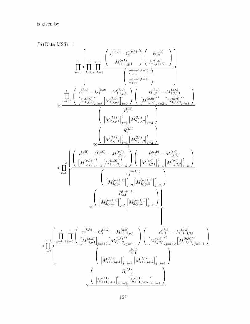
is given by
Pr(Data|MSS) =
l∏
ν=0
1∏
k=0
t−1∏
i=k+1
r(ν,k)i − O
(ν,k)i
M(ν,k)i,i+1,p,1
R(ν,k)i,2
M(ν,k)i,i+1,2,1
T
(ν+1,k+1)i+1
C(ν+1,k+1)i+1
×
l∏
h=l−1
r(h,0)1 − O
(h,0)1 −M
(h,0)1,2,p,1[
M(h,0)1,j,p,1
]tj=3
[M
(h,0)1,j,p,2
]tj=2
R(h,0)1,2 −M
(h,0)1,2,2,1[
M(h,0)1,j,2,1
]tj=3
[M
(h,0)1,j,2,2
]tj=2
r(l,1)2[
M(l,1)2,j,p,1
]tj=3
[M
(l,1)2,j,p,2
]tj=2
×
R(l,1)2,1[
M(l,1)2,j,1,1
]tj=3
[M
(l,1)2,j,1,2
]tj=2
1
×l−2∏
ν=0
r(ν,0)1 − O
(ν,0)1 −M
(ν,0)1,2,p,1[
M(ν,0)1,j,p,1
]tj=3
[M
(ν,0)1,j,p,2
]tj=2
R(ν,0)1,2 −M
(ν,0)1,2,2,1[
M(ν,0)1,j,2,1
]tj=3
[M
(ν,0)1,j,2,2
]tj=2
r(ν+1,1)2[
M(ν+1,1)2,j,p,1
]tj=3
[M
(ν+1,1)2,j,p,2
]tj=2
×
R(ν+1,1)2,1[
M(ν+1,1)2,j,1,1
]tj=3
[M
(ν+1,1)2,j,1,2
]tj=2
1
×t−2∏
i=2
l∏
h=l−1
1∏
k=0
r(h,k)i −O
(h,k)i −M
(h,k)i,i+1,p,1[
M(h,k)i,j,p,1
]tj=i+2
[M
(h,k)i,j,p,2
]tj=i+1
R(h,k)i,2 −M
(h,k)i,i+1,2,1[
M(h,k)i,j,2,1
]tj=i+2
[M
(h,k)i,j,2,2
]tj=i+1
r(l,1)i+1[
M(l,1)i+1,j,p,1
]tj=i+2
[M
(l,1)i+1,j,p,2
]tj=i+1
×
R(l,1)i+1,1[
M(l,1)i+1,j,1,1
]tj=i+2
[M
(l,1)i+1,j,1,2
]tj=i+1
1
167

×l−2∏
ν=0
1∏
k=0
r(ν,k)i − O
(ν,k)i −M
(ν,k)i,i+1,p,1[
M(ν,k)i,j,p,1
]tj=i+2
[M
(ν,k)i,j,p,2
]tj=i+1
R(ν,k)i,2 −M
(ν,k)i,2,2,1[
M(h,k)i,j,2,1
]tj=i+2
[M
(h,k)i,j,2,2
]tj=i+1
r(ν+1,1)i[
M(ν+1,1)i+1,j,p,1
]tj=i+2
[M
(ν+1,1)i+1,j,p,2
]tj=i+1
×
R(ν+1,1)i+1,1[
M(ν+1,1)i+1,j,1,1
]tj=i+2
[M
(ν+1,1)i+1,j,1,2
]tj=i+1
1
.
The generalization of the age-dependence model goodness-of-fit test involves
additional terms arising from the partitioning of the data according to recapture
status on capture at i (i.e. recapture vs first capture). Because of the extensive
splitting of the data set, first by age classes and second according to recapture
status, the parameter estimates will tend to have low precision, except in large-
scale tagging programs such as some fisheries experiments. Of greatest interest
may be the tests between models. These will be of two types, according to the
null-hypothesis H0: age-dependence or H0: marking effect.
For the first test, H0: age-dependence vs H1: age-dependence and marking
effect, the conditional distribution PrH0(S|S) where (S and S) are the MSS for
H1 and H0 respectively is given by
PrH0(S|S) =
l∏
ν=1
t∏
i=2
1∏
k=0
N
(ν,k)i
R(ν,k)i,1
N(ν)i
Ri,1(ν)
t−1∏
i=2
1∏
k=0
n
(ν,k)i
R(ν,k)i,2
n
(ν)i
R(ν)i,2
×t−1∏
i=2
1∏
k=0
r(ν,k)i
O(ν,k)i
r(ν)i
O(ν)i
t−1∏
i=3
2∏
k=1
T
(ν+1,k)i
C(ν+1,k)i
T
(ν+1)i
C(ν+1)i
.
168

Note that age-class 0 animals make no contribution to this test as there are no
observations of age class 0 animals in mark class 1.
For the second test, H0: marking effect vs H1: age-dependence and marking
effect, PrH0(S|S) is given by
PrH0(S|S) =
1∏
k=0
t∏
i=2
l∏
ν=k
N
(ν,k)i
R(ν,k)i,1
N
(k)i
R(k)i,1
t−1∏
i=2
l∏
ν=k
n
(ν,k)i
R(ν,k)i,2
n
(k)i
R(k)i,2
×t−1∏
i=2
l∏
ν=k
r(ν,k)i
O(ν,k)i
r(k)i
O(k)i
t−1∏
i=3
l+1∏
ν=k+1
T
(ν,k+1)i
C(ν,k+1)i
T
(k+1)i
C(k+1)i
.
Including the tests developed for just the age-dependence and marking effect
models we have alternative pathways for hypothesis testing, each testing the se-
quence Model 1 v Model 2 v Model 3. In both pathways, Model 1 is the one age
model without marking effect and Model 3 has both types of dependence. In one
pathway Model 2 has just a marking effect and in the other pathway Model 2 has
just age-dependence. Within each pathway the tests are nested, however tests are
not nested between pathways. It is possible that both the tests of age-dependence
and marking effect vs the one-age model with no marking effect are significant, but
that neither are significant when the comparison is with the marking effect and age-
dependence model. In such cases the experimenters must rely on their judgement
based on an understanding of the biology of the animals as to which generalization
may be more appropriate, although Akaike’s Information Criterion (Lebreton et al.
1992) may be useful as an objective means of differentiating between models. Note
several publications deal specifically with the use of this model selection criterion in
open mark-recapture models (Anderson et al. 1994, Burnham and Anderson 1992,
Burnham et al. 1994,1995a,1995b).
169

4.5 Observations Obtained After t
In many studies resightings may be obtained after time t, up to time v, where time
t is the final period in which animals were captured. This is particularly likely
when observations of marked animals are reported by members of the public. To
obtain estimates as efficiently as possible, these observations should be included in
the analysis.
Because there are no recaptures after time t, and also because of the age-
dependence, there are some important structural limitations to the data. These
are:
• There are no C(ν,k)i,1 or C
(ν,0)i,2 cohorts for i > t and for any ν or k.
• For ν < l, additional C(ν,1)i,2 release cohorts can only occur for i = t, ..., t + ν.
At times greater than t + ν all marked animals are known to be older than
age ν.
• For ν = l additional C(ν,1)i,2 release cohorts can only occur for i = t, ..., v − 1.
In addition we have the usual restriction that there are no C(0,1)i cohorts, because
marked animals of age 0 cannot be captured, and there are also, by definition, no
C(ν,1)1 cohorts (ν = 1, ..., l) (i.e. no releases of marked animals in mark class 1 at
time 1).
4.5.1 Probability structure under random emigration
Let
ωx = min(l, ν + x− i) .
For i = 1, ..., t and j = t + 1,...,v the probability structure for observations of
members of C(ν,k)i,1 is given by
π(ν,k)i,j,1,2 = α
(ωj ,1)j,2 β
(ν,k)i
j−1∏
h=i+1
β(ωh,1)h ,
170

where α(ν,1)j,2 = f
(ν,1)j and β
(ν,k)t is defined as in (4.18). Because animals are not
captured after t, β(ν,1)j is given by
β(ν,1)j = S
(ν,k)i θ
(ν,k)i j = t+ 1, ..., v − 1 .
Now for j > t the parameters α(ωj ,1)j,2 , and β
(ωt,1)t ,β
(ωt+1,1)t+1 ,..., β
(ωj−1,1)j−1 always occur
in the product
α(ωj ,1)j,2 β
(ν,k)i
j−1∏
h=i+1
β(ωh,1)h
hence these parameters are not individually identifiable. Instead we define the
parameters
ξ(ν,k)j = α
(ωj ,1)j,2 β
(ν,k)t
j−1∏
h=t+1
β(ωh,1)h ,
and for j = t+ 1, ..., v re-write the observation probabilities as
π(ν,k)i,j,1,2 =
β(ν,k)i
t−1∏
h=i+1
β(ωh,1)h ξ
(ωj−1,1)j i = 1, ..., t− 1
ξ(ν,k)j i = t
.
For i = 1, ..., t and j = t + 1,...,v the probability structure for observations of
members of C(ν,k)i,2 is given by
π(ν,k)i,j,2,2 = δ
(ν,k)i π
(ν,k)i,j,1,2 .
However, for i = t+1, ..., t+ν (t+ν < l) or i = t+1, ..., v−1 (ν = l) the probability
structure for observations of members of C(ν,1)i,2 is given by
π(ν,1)i,j,2,2 = δ
(ν,1)i α
(ωj ,1)j,2
j−1∏
h=i
β(ωh,1)h . (4.25)
As with ξ(ν,k)j the parameters in the product (4.25) are completely confounded.
4.5.2 Additional components to the likelihood under ran-
dom emigration
If we have observations of marked animals from beyond the final capture period
then after the t− 1th “peeling” and “pooling” cycle we are left with the term
Pr(M(0,0)t,t,1,2, ...,M
(0,0)t,v,1,2|R
(0,0)t,1 )
171

×l∏
ν=1
1∏
k=0
r(ν,k)t−1 − O
(ν,k)t−1 − C
(ν,k+1)t[
M(ν,k)t−1,j,p,2
]vj=t
R
(ν,k)t−1,2 −M
(ν,k)t−1,t,2,2[
M(ν,k)t−1,j,2,2
]vj=t
R(ω,1)t,1[
M(ω,1)t,j,2,2
]vj=t
r(ω,1)t[
M(ω,1)t,j,p,2
]vj=t
×Pr(M
(ν,k)t,t,p,2, ...,M
(ν,k)t,v,1,2|r
(ν,k)t )
×l∏
ν=0
Pr(Mν,0)t,t+1,2,2, ...,M
(ν,0)t,v,2,2|R
(ν,0)t,2 )
×l−1∏
ν=1
t+ν∏
i=t
Pr(M(ν,1)i,i+1,2,2, ...,M
(ν,1)i,v+1,2,2)
×v−1∏
i=t
Pr(Ml,1)i,i+1,2,2, ...,M
(l,1)i,v+1,2,2) ,
where M(ν,1)i,v+1,2,2 is the number of animals released at i following observation in age
class ν that were never observed again.
If we define the additional statistics as follows
r(ν,0)t = R
(ν,0)t,1
Oν,0)t = M
(ν,0)t,t,1,2
M(ν,0)t,j,p,2 = M
(ν,0)t,j,1,2
then factoring observations for the tth release cohorts we find for k = 0 and ν =
0, ..., l, or k = 1 and ν = 1, ..., l
P r(M(ν,k)t,t,p,2, ...,M
(ν,k)t,v,p,2|r
(ν,k)t )
= Pr(M(ν,k)t,t,p,2|r
(ν,k)t )Pr(M
(ν,k)t,t+1,p,2, ...,M
(ν,k)t,v,p,2|r
(ν,k)t −M
(ν,k)t,t,p,2)
where
(M(ν,k)t,t,p,2|r
(ν,k)t ) = (O
(ν,k)t |r
(ν,k)t )
is binomial B(r(ν,k)t , τ
(ν,k)t,2 ),
τ(ν,k)t,2 =
α(ν,k)t,2
λ(ν,k)t,2
.
172

Also,
(M(ν,k)t,t+1,1,2, ...,M
(ν,k)t,v,1,2|r
(ν,k)t −O
(ν,k)t )
is multinomial with conditional cell probabilities
ξ(ν,k)j
v∑
h=t+1
ξ(ν,k)h
for j = t + 1, ..., v. For ν = 0, ..., l:
Pr(M(ν,k)t,t+1,2,2, ...,M
(ν,k)t,v,2,2|R
(ν,k)t,2 )
is multinomial with conditional cell probabilities
δ(ν,k)t ξ
(ν,k)j
δ(ν,k)t
v∑
h=t+1
ξ(ν,k)h
=ξ
(ν,k)j
v∑
h=t+1
ξ(ν,k)h
for j = t+ 1, ..., v, hence observations of (M(ν,k)t,t+1,2,2, ...,M
(ν,k)t,v,2,2|R
(ν,k)t,2 ) can be pooled
with (M(ν,k)t,t+1,1,2, ...,M
(ν,k)t,v,1,2|r
(ν,k)t − O
(ν,k)t ). Thus we obtain the additional terms in
the likelihoodn
(0,0)t
R(0,0)t,2
(λ
(0,0)t,2
)R(0,0)t,2
(1 − λ
(0,0)t,2
)n(0,0)t −R
(0,0)t,2
×l∏
ν=1
1∏
k=0
n
(ν,k)t
R(ν,k)t,2
(λ
(ν,k)t,2
)R(ν,k)t,2
(1 − λ
(ν,k)t,2
)n(ν,k)t −R
(ν,k)t,2
×
r(0,0)t
O(0,0)t
(τ
(0,0)t,2
)O(0,0)t
(1 − τ
(0,0)t,2
)r(0,0)t −O
(0,0)t
×l∏
ν=1
1∏
k=0
r(ν,k)t
O(ν,k)t
(τ
(ν,k)t,2
)O(ν,k)t
(1 − τ
(ν,k)t,2
)r(ν,k)t −O
(ν,k)t
×
r(0,0)t −O
(0,0)t
[M
(0,0)t,j,1,2
]vj=t+1
R(0,0)t,2[
M(0,0)t,j,2,2
]vj=t+1
r(0,0)t −O
(0,0)t +R
(0,0)t,2[
M(0,0)t,j,.,2
]vj=t+1
173

×
r(0,0)t −O
(0,0)t +R
(0,0)t,2[
M(0,0)t,j,.,2
]vj=t+1
v∏
j=t+1
ξ(0,0)j
v∑
h=t+1
ξ(0,0)h
M(0,0)t,j,.,2
×l∏
ν=1
1∏
k=0
r(ν,k)t −O
(ν,k)t
[M
(ν,k)t,j,1,2
]vj=t+1
R(ν,k)t,2[
M(ν,k)t,j,2,2
]vj=t+1
r(ν,k)t − O
(ν,k)t +R
(ν,k)t,2[
M(ν,k)t,j,.,2
]vj=t+1
×
r(ν,k)t − O
(ν,k)t +R
(ν,k)t,2[
M(ν,k)t,j,.,2
]vj=t+1
v∏
j=t+1
ξ(ν,k)j
v∑
h=t+1
ξ(ν,k)h
M(ν,k)t,j,.,2
×l∏
ν=1
min(t+ν,v−1)∏
i=t+1
nν,ki[
M(ν,k)i,j,2,2
]v+1
j=i+1
v+1∏
j=i+1
(π
(ν,1)i,j,2,2
)M(ν,1)i,j,2,2
where
M(ν,k)t,j,.,2 = M
(ν,k)t,j,1,2 +M
(ν,k)t,j,2,2 .
4.5.3 Additional parameter estimates under random emi-
gration
Due to the additional observations, we have extra parameters to estimate. In
addition, the parameter τ(ν,k)t,2 is defined and estimation of this parameter now con-
tributes to the estimation of f(ν,k)t . From
τ(ν,k)t,2 =
αν,k)t,2
λ(ν,k)t,1
=f
(ν,k)t
λ(ν,k)t,1
,
and substituting the MLE’s for τ(ν,k)t,2 and λ
(ν,k)t,1 we obtain
f(ν,k)t = λ
(ν,k)t,1 τ
(ν,k)t,2
=R
(ν,k)t,1
N(ν,k)t
O(ν,k)t
r(ν,k)t
174

and is identical to (4.21) for i 6= t.
We can also estimate θ(ν,k)t . From
λ(ν,k)t,2 = δ
(ν,k)t (λ
(ν,k)t,1 − α
(ν,k)t,2 )
we obtain
θ(ν,k)t =
1 − τ(ν,k)t,2
1 + τt,2(λt,2 − 1).
Substituting the MLE’s for τ(ν,k)t,2 , and λ
(ν,k)t,2 we obtain
θ(ν,k)t =
n(ν,k)t
(r(ν,k)t −O
(ν,k)t
)
r(ν,k)t n
(ν,k)t +O
(ν,k)t
(R
(ν,k)t,2 −n
(ν,k)t
)
which is identical to (4.22) but with i = t. Asymptotic variances for f(ν,k)t and θ
(ν,k)t
are given by (4.23) and (4.24) respectively (in the case of f(ν,k)t substituting t for i
in (4.23)).
In addition to f(ν,k)t and θ
(ν,k)t we can estimate values for the parameters ξ
(ν,k)i and
π(ν,k)i,j,2,2. However, because they represent products of confounded parameters they
are of little direct interest, although they may have a use for computing expected
values in order to assess model fit (Brownie et al. 1985:17).
Since (M(ν,k)t,t+1,.,2, ...,M
(ν,k)t,v,.,2|r
(ν,k)t −O
(ν,k)t +R
(ν,k)t,2 ) is multinomial with conditional
cell probabilities
π∗(ν,k)j =
ξ(ν,k)j
v∑
h=t+1
ξ(ν,k)h
=ξ
(ν,k)j
λ(ν,k)t,1 − α
(ν,k)t,2
,
substituting MLEs’ for π∗(ν,k)j , λ
(ν,k)t,1 , and f
(ν,k)t = α
(ν,k)t,2 we obtain
ξ(ν,k)j =
M(ν,k)t,j,.,2
(r(ν,k)t − O
(ν,k)t +R
(ν,k)t,2 )
R(ν,k)t,1
N(ν,k)t
(r(ν,k)t − O
(ν,k)t )
r(ν,k)t
.
Because the π(ν,k)i,j,2,2 simply represent the cell probabilities for the M
(ν,1)i,j,2,2’s their
MLE’s are given by
π(ν,1)i,j,2,2 =
M(ν,1)i,j,2,2
n(ν,1)i
i = t + 1, ..., ν − 1; j = i+ 1, ..., v .
175

4.5.4 Additional components to the goodness-of-fit tests
When v > t we have an additional component to the residual Pr(Data|MSS) after
factorization cycle t. This term is used in goodness of fit testing and is given
r(0,0)t−1 −O
(0,0)t−1 − C
(0,1)t
[M
(0,0)t−1,j,p,2
]vj=t
R
(0,0)t−1,2 −M
(0,0)t−1,t,2,2[
M(0,0)t−1,j,2,2
]vj=t
R(1,1)t,1[
M(1,1)t,j,2,2
]vj=t
r(1,1)t[
M(1,1)t,j,p,2
]vj=t
×l−2∏
ν=1
1∏
k=0
r(ν,k)t−1 − O
(ν,k)t−1 − C
(ν,k+1)t[
M(ν,k)t−1,j,p,2
]vj=t
R
(ν,k)t−1,2 −M
(ν,k)t−1,t,2,2[
M(ν,k)t−1,j,2,2
]vj=t
R(ν+1,1)t,1[
M(ν+1,1)t,j,2,2
]vj=t
r(ν+1,1)t[
M(ν+1,1)t,j,p,2
]vj=t
×1∏
k=0
l−2∏
ν=1
r(ν,k)t−1 −O
(ν,k)t−1 − C
(ν,k+1)t[
M(ν,k)t−1,j,p,2
]vj=t
R
(ν,k)t−1,2 −M
(ν,k)t−1,t,2,2[
M(ν,k)t−1,j,2,2
]vj=t
R(l,1)t,1[
M(l,1)t,j,2,2
]vj=t
r(l,1)t[
M(l,1)t,j,p,2
]vj=t
.
These terms give rise to an additional 2l−1 conditionally independent contingency
tables. In addition, factorization cycle t gives rise to the term
r(0,0)t −O
(0,0)t
[M
(0,0)t,j,1,2
]vj=t+1
R(0,0)t,2[
M(0,0)t,j,2,2
]vj=t+1
r(0,0)t −O
(0,0)t +R
(0,0)t,2[
M(0,0)t,j,.,2
]vj=i+1
×l∏
ν=1
1∏
k=0
r(ν,k)t −O
(0,0)t
[M
(ν,k)t,j,1,2
]vj=t+1
R(ν,k)t,2[
M(ν,k)t,j,2,2
]vj=t+1
r(ν,k)t − O
(ν,k)t +R
(ν,k)t,2[
M(ν,k)t,j,.,2
]vj=i+1
,
leading to an additional 2l + 1 conditionally independent contingency tables.
176

4.5.5 Age-dependence and marking effect models under per-
manent and Markov emigration with v > t
Under permanent and random emigration computation of observation cell proba-
bilities makes use of γ(ν,k)i,j,1 , the probability an animal released at time i as a member
of age class ν and mark class k is not recaptured between i and j, nor at j. Because
we do not capture animals after t we find
γ(ν,k)i,j =
γ
(ν,k)i,t i = 1, ..., t− 1 , j = t+ 1, ..., v
1 i = t. (4.26)
In addition to the parameters that can be estimated when v = t we can estimate
the parameters ξ(ν,k)i (i = t+ 1, ..., v) and π
(ν,1)i,j,2,2 (i = t+ 1, ..., v− 1 j = t+ 1, ..., v).
These products of confounded parameters are defined exactly as under random
emigration.
177

178

Chapter 5
Modified and Reduced Parameter
Models
In this section we consider a number of important reduced parameter versions of
the models discussed in Chapters 3 and 4. In some cases these reduced parameter
models lead to closed form MLE’s that correspond to published mark-recapture
estimators. In other cases reduced parameter models do not lead to closed-form
solutions and we discuss how these models can be fitted.
5.1 Models with No Resightings
If we make the constraint f(ν,k)i = (1 − θ
(ν,k)i ) = 0 then the M
(ν,k)i,j,m,2 (m=1,2) and
hence O(ν,k)i , and n
(ν,k)i are all structurally zero. If we also assume that emigration
is permanent (in the age-dependent model including one-age as a special case)
or random (in the single age class model only) and omit the subscripts used to
denote the type of release cohort we find that the estimators of survival and capture
probabilities and their respective variances reduce to
S(ν,k)i =
R(ν,k)i
N(ν,k)i r
(ν,k)i
N
(ω,1)i+1 Z
(ν+1,k+1)i+1
R(ω,1)i+1
+ C(ν+1,k+1)i+1
,
V ar(S(ν,k)i ) = (S
(ν,k)i )2
1
E[R(ν,k)i ]
−1
N(ν,k)i
+ (1 − p∗(ν,k)i+1 )2
1
E[R(ω,1)i+1 ]
−1
N(ω,1)i+1
179

+ p∗(ν,k)i+1 (1 − p
∗(ν,k)i+1 )
(N(ω,1)i+1 − E[R
(ω,1)i+1 ])2
N(ω,1)i+1 E[R
(ω,1)i+1 ]E[T
(ν+1,k+1)i+1 ]
ˆp∗(ν,k)i =
C(ν+1,k+1)i
N(ω,1)i
Z(ν+1,k+1)i
R(ω,1)i
+ C(ν+1,k+1)i
i = 2, ..., t
and
V ar(p∗(ν,k)i ) =
[p∗(ν,k)i (1 − p
∗(ν,k)i )
]2(
1
E[R(ω,1)i ]
−1
N(ω,1)i
+1
E[C(ν+1,k+1)i ]
+1
Z(ν+1,k+1)i
)
which in the one-age case with no marking effect are the Jolly-Seber estimators of
Si = φi and p∗i = pi.
Importantly, in the single age-class case we are unable to discriminate between
the case of random emigration or permanent emigration as the probability structure
for the model is identical in either case (Burnham 1993). The type of emigration
does effect the interpretation of the parameters however. For example, if emigration
is permanent in the one-age model without a marking effect then p∗i = pi and Si =
SiFi is the joint probability a marked animal survives from i, i + 1 and is at risk
of capture at i + 1. If emigration is random, then p∗i = piFi−1 and Si is the true
survival rate.
In the age-dependent model we can distinguish between the two models. If
we have the age-dependent model under permanent emigration and no ancillary
observations and no marking effect then the model reduces to that developed by
Pollock (1981). To simplify the discussion we will just consider the two-age case.
For this model, under permanent emigration a minimal sufficient statistic is given
by R(0)i (i=1,...t−1), R
(1)i (i=1,...,t−1), and Ci (i=2,...,t−1) (Brownie et al. 1986)
where Ci is the total number of animals captured at i. This sufficient statistic has
dimension 3t− 4 with 3t− 4 estimable parameters given in closed-form by Pollock
et al. (1990).
Under random emigration, however, we find from 4.11 that a MSS is given by
R(0)i (i=1,...,t − 1), R
(1)i (i=1,...,t − 1), C
(1)i (i=2,...,t − 1) and C
(2)i (i=2,...,t − 1)
180

which has dimension 4t− 6 with 4t− 6 estimable parameters in the model. Closed-
form solutions to the p∗(ν)i and S
(ν)i ’s are given in Chapter 4. The additional t− 1
identifiable parameters in the random emigration model when compared to the
permanent emigration model are p∗(0)i (i = 2, ..., t−1) and p
∗(0)t St. Thus the models
lead to different likelihoods and different parameter estimates. Moreover if we
examine the probability structure (Tables 5.1 and 5.2) we find that the permanent
emigration model is in fact a constrained version of the random emigration model.
If in the random emigration model (Table 5.1) we make the constraint p∗(0)i = p
∗(1)i
(i = 2,...,t − 1) then we obtain a reduced model which is identical in structure to
the permanent emigration model developed by Pollock (1981).
Table 5.1: Probability structure for a t = 4 two-age Jolly-Seber model with no
marking effect under random emigration where p∗(1)i = F
(1)i−1p
(1)i and p
∗(0)i = F
(0)i−1p
(1)i .
j=2 3 4
Adults
i=1 S(1)1 p
∗(1)2 S
(1)1 (1 − p
∗(1)2 )S
(1)2 p
∗(1)3 S
(1)1 (1 − p
∗(1)2 )S
(1)2 (1 − p
∗(1)3 )S
(1)3 p
∗(1)4
2 S(1)2 p
∗(1)3 S
(1)2 (1 − p
∗(1)3 )S
(1)3 p
∗(1)4
3 S(1)3 p
∗(1)4
Young
i=1 S(0)1 p
∗(0)2 S
(0)1 (1 − p
∗(0)2 )S
(1)2 p
∗(1)3 S
(0)1 (1 − p
∗(0)2 )S
(1)2 (1 − p
∗(1)3 )S
(1)3 p
∗(1)4
2 S(0)2 p
∗(0)3 S
(0)2 (1 − p
∗(0)3 )S
(1)3 p
∗(1)4
3 S(0)3 p
∗(0)4
The structural equivalence between the constrained random emigration model
and the permanent emigration model means that we can formally test the null hy-
pothesis that emigration is permanent against the alternative of random emigration.
From Brownie et al. (1986) the log-likelihood function (ignoring the normalizing
constant) for the recaptures of marked animals in a two-age Jolly-Seber model
under permanent emigration with no marking effect is given by
Lp =∑
ν=
{t−∑
i=
R(ν)i ln(λ
(ν)i,p ) + (N
(ν)i −R
(ν)i ) ln(− λ
(ν)i,p )
}+
t−∑
i=
Ci ln(τi,p)Zi ln(− τi,p)
181

Table 5.2: Probability structure for a t = 4 two-age Jolly-Seber model with no
marking effect under permanent emigration where S∗(ν)i = S
(ν)i F
(ν)i .
j=2 3 4
Adults
i=1 S∗(1)1 p
(1)2 S
∗(1)1 (1 − p
(1)2 )S
∗(1)2 p
(1)3 S
∗(1)1 (1 − p
(1)2 )S
∗(1)2 (1 − p
(1)3 )S
∗(1)3 p
(1)4
2 S∗(1)2 p
∗(1)3 S
∗(1)2 (1 − p
(1)3 )S
∗(1)3 p
(1)4
3 S∗(1)3 p
(1)4
Young
i=1 S∗(0)1 p
(1)2 S
∗(0)1 (1 − p
(1)2 )S
∗(1)2 p
(1)3 S
∗(0)1 (1 − p
1)2 )S
∗(1)2 (1 − p
(1)3 )S
∗(1)3 p
(1)4
2 S∗(0)2 p
1)3 S
∗(0)2 (1 − p
1)3 )S
∗(1)3 p
(1)4
3 S∗(0)3 p
(1)4
where Ci = C(1)i +C
(2)i , Zi = Z
(1)i +Z
(2)i . From Chapter 4 the log-likelihood function
under the random emigration model (ignoring the normalizing constant) is given
by
Lr =1∑
ν=0
t−1∑
i=1
R(ν)i ln(λ
(ν)i,r ) + (N
(ν)i −R
(ν)i ) ln(1 − λ
(ν)i,r )
+t−1∑
i=2
C(ν+1)i ln(τ
(ν+1)i,r )Z
(ν+1)i ln(1 − τ
(ν+1)i,r ) .
Noting that λ(ν)i,p = λ
(ν)i,r , τi,p = Ci
Ti, and τ
(ν)i,r =
C(ν)i
T(ν)i
, where Ti = Zi +Ci, we find that
the log-likelihood-ratio test statistic is given by
X2 = −2t−1∑
i=2
Ci ln(
Ci
Ti
) + Zi ln(Zi
Ti
) −2∑
ν=1
C(ν)i ln(
C(ν)i
T(ν)i
) + Z(ν)i ln(
Z(ν)i
T(ν)i
)
= −2t−1∑
i=2
2∑
ν=1
C(ν)i ln(
C(ν)i Ti
ZiT(ν)i
) + Z(ν)i ln(
Z(ν)i Ti
ZiT(ν)i
) ,
with t− 2 degrees of freedom.
Alternatively we can construct contingency tables to test between models. If S
is the set of minimally sufficient statistics under the null, permanent emigration,
model and S is the set of minimally sufficient statistics under the alternative,
182

random emigration, model then
Pr(S|S) =t−∏
i=
C
(1)i
T(1)i
C
(2)i
T(2)i
Ci
Ti
leading to the set of t− 2 conditionally independent contingency tables of the form
given in Table 5.3. As discussed in Chapter 4 the contingency table approach is
Table 5.3: Contingency table used to test the “random” vs “permanent” emigration
models
Young at i− 1, Adult at i− 1,
captured at i or after i captured at or after i
Captured at i C(1)i C
(2)i Ci
Not captured at i+ 1 Z(1)i Z
(2)i Zi
T(1)i T
(2)i Ti
generally preferred if “exact” significance can be assessed using the hypergeometric
distribution. If a chi-square approximation is used instead of the exact procedure,
then the contingency table and likelihood ratio tests would have the same asymp-
totic power.
Although we have described the test as a comparison of the “permanent” and
the “temporary” emigration models, we are really testing whether age-group at
i − 1 has an effect on capture probability at i. This test will be sensitive to any
mechanism that leads to such an age-group dependence. Random emigration is just
one particularly important alternative that leads to capture probabilities at time i
differing between animals who were young at i−1 and those animals who were adult
at i − 1. Therefore rejection of the permanent emigration model in favour of the
random emigration should not be taken as strict evidence of random emigration.
Rather rejection of the permanent emigration assumption is simply evidence of age-
dependent capture probabilities, with a number of possible explanations including
random emigration.
183

In contrast, in the full model (i.e. with resightings) the permanent emigration
model has more estimable parameters than the random emigration model. More-
over, the two models are no longer nested and we have no formal test for discrimi-
nating between the two models. Note, however, if we make the constraint F(ν,k)i = 1
(i.e. no emigration) in the one age-class permanent emigration model we obtain a
probability structure that is identical to the random emigration model, with the
difference that p∗(ν,k)i = p
(ν,k)i . Thus, in the one age-class case the likelihood ratio
test between the permanent emigration and no-emigration models (F(ν,k)i = 1) is in
fact a test of the composite “either no, or random, emigration” hypothesis against
the alternative of permanent emigration.
Finally, if the random emigration age-dependence model is valid, then we can
use our estimator of p∗(ν,k)i to estimate the relative movement rates ρ
(k)i of animals
in the oldest two age classes. Since
p∗(l−1,k)i+1 = F
(l−1,k)i p
(l,k)i+1
and
p∗(l,k)i+1 = F
(l,k)i p
(l,k)i+1
then
ρ(k)i =
F
(l,k)i
F(l−1,k)i
=p∗(l,k)i+1
p∗(l−1,k)i+1
.
with asymptotic variance
V ar(ρ(k)i ) =
V ar(p∗(l,k)i+1[
p∗(l−1,k)i+1
]2 +
[V ar(p
∗(l,k)i+1
]2p∗(l−1,k)i+1
[p∗(l−1,k)i+1
]4 −2[p∗(l,k)i+1
]2Cov(p
∗(l,k)i+1 p
∗(l−1,k)i+1 )
[p∗(l−1,k)i+1
]3 .
However, this estimator may not be very useful as it depends on the assumption
that animals in age class l and mark class k at time i have the same capture
probabilities regardless of their age class at time i− 1.
184

5.1.1 Benefit of including ancillary observations
Relative efficiency of the survival rate estimator
Using our closed-form expressions for the variance of the parameter estimates un-
der random emigration we can compare the relative efficiency of the survival rate
estimator under the Jolly-Seber model with the survival rate estimator obtained
using our model. This is easily done by generating expected values of the statistics
under particular parameter combinations then substituting these expected values
into the variance expressions.
For simplicity, a single age-class t = 5 study with all parameters equal through
time (although not structurally constrained) was considered. In addition the obser-
vation and death processes was constrained so that death followed a homogeneous
Poisson process, and first observation within (i, i + 1) a non-homogeneous process
with heterogeneity due entirely to the death of individuals. In this case it can be
shown (Terry Moore pers. comm.) that
θi = (1 − fi)ln(Si)
Si−1 . (5.1)
Denoting Si as the estimate obtained with ancillary observations and SJSi as
the estimate of Si under the Jolly-Seber model using the same data, but without
ancillary observations, relative efficiency was measured by
V ar(SJSi )
V ar(Si).
This was computed only for estimates of S1, S2, and S3 as no estimate of S4 is
possible in a t = 5 Jolly-Seber model. Note that the measure of relative efficiency
is based on V ar(Si|Si). This is the only component of the survival probability
variance estimate that is affected by the inclusion of ancillary observations.
Relative efficiency was an increasing function of p, f , and i (Tables 5.1, 5.2,
and 5.3), and always greater than one. Relative efficiency for larger values of f
was not as great when p was also large. Higher survival rate appears to elevate the
rate at which relative efficiency increased with the observation probability (i.e. an
increase in the second derivative of relative efficiency with respect to f), and as a
185

consequence the increase in relative efficiency with i was also greater for the higher
survival rates.
Intuitively, including ancillary observations improves the survival rate estimates
because we obtain observations on animals that were never captured following re-
lease. Without ancillary observations these animals do not contribute to Ri,1 or
Zi. Thus efficiency will be improved by influences, such as increasing fi, which
lead to an increase in the expected values of Ri,1 and Zi. The relative increase in
E[Ri,1] and E[Zi] resulting from the inclusion of ancillary observations would be
greatest when p was small relative to f . For example in a study where p was close
to 1, there would be a relatively small gain from including ancillary observations as
most live animals are recaptured in any case. Similarly E[Ri,1] and E[Zi] increase
with t thus the relative benefit of including ancillary observations would be greater
in short rather than long studies. This is evident from Table 5.4 where relative
efficiency with various f , S, and p are given for estimates of S1, S2, and S3 in a
t = 10 study, however the difference between a t = 5 and t = 10 study appears
slight.
The effect of heterogeneous capture probabilities
An important assumption of the Jolly-Seber model and the extensions to it that we
have considered in Chapter 3 is that all animals have the same capture probability
at time i - the homogeneous capture probability assumption. As we have shown in
Chapter 4 we can relax this assumption and allow animals to have different capture
probabilities according to known classes of animals. In some cases there may be
inherent heterogeneity with some animals more or less vulnerable to capture as a
consequence of factors that can be difficult to explicitly incorporate in the model.
For example poorly conditioned animals may have higher capture probabilities if
traps are baited with food. These animals may also have lower survival rates.
The effects of heterogeneous capture probabilities on the Jolly-Seber estimators
are well known (see section 1.4.4). Essentially, the marked members of the pop-
ulation will tend to be those with high capture probabilities, and the estimate of
186

Figure 5.1: Relative asymptotic efficiency of the survival rate estimator of the one-
age mark recapture model with ancillary observations relative to the Jolly-Seber
model with t = 5 and Si = 0.3 (Relative efficiency =V ar(SJS
i)
V ar(Si)).
187

Figure 5.2: Relative asymptotic efficiency of the survival rate estimator of the one-
age mark recapture model with ancillary observations relative to the Jolly-Seber
model with t = 5 and Si = 0.5 (Relative efficiency =V ar(SJS
i)
V ar(Si)).
188

Figure 5.3: Relative asymptotic efficiency of the survival rate estimator of the one-
age mark recapture model with ancillary observations relative to the Jolly-Seber
model with t = 5 and Si = 0.8 (Relative efficiency =V ar(SJS
i)
V ar(Si)).
189

Figure 5.4: Relative asymptotic efficiency of the survival rate estimator of the one-
age mark recapture model with ancillary observations relative to the Jolly-Seber
model with t = 10 and various survival and capture probabilities (Relative efficiency
=V ar(SJS
i)
V ar(Si)).
190

subsequent capture probability will as a consequence also be high. This in turn
will lead to under-estimation of the size of the population. Bias of the survival rate
estimator, although non-zero, is generally small.
If the method of obtaining observations is unrelated to the capture method
then individual capture probabilities may be unrelated to the probability a marked
animal is observed. In these circumstances we might expect that the effect of hetero-
geneous capture probabilities is reduced by the inclusion of ancillary observations as
we rely less on physical capture of the animals in collecting information on marked
animals. In addition we expect the survival rate estimator to have even less bias
as we are able to obtain information on the survival of low capture probability
individuals through the observation process.
To examine the effect of heterogeneous capture probabilities on the estimators
the expected values of the statistics Ri,1, Ci, and Zi were obtained from a one-age
mark-recapture study under random emigration with ancillary observations and
where all animals are released on observation. The animal population was made up
of low and high capture probability individuals with capture probabilities pl and ph
respectively. The extent of heterogeneity was measured by the parameter ∆p, where
pl = p− ∆p
2and ph = p+ ∆p
2. All remaining parameters were held constant through
time (although not constrained in the model), with θi given by 5.1. Asymptotic
bias in the capture and survival rate estimators relative to the asymptotic bias of
the Jolly-Seber estimators was measured for various combinations of p, S, f , and
∆p. Relative asymptotic bias (relative bias) was measured by
Relative bias =p∗i − p
p∗JSi − p
,
where p∗i is the capture probability estimate in the model with ancillary observa-
tions assuming random emigration and p∗JSi the corresponding Jolly-Seber capture
probability estimate obtained from the same data by ignoring resightings.
As suggested above, mark-recapture estimators incorporating ancillary observa-
tion appear to be more robust to heterogeneous capture probabilities (Figures 5.5,
5.6, 5.7, and 5.8) with relative bias of capture probability and survival rate esti-
191

mates reduced by the inclusion of ancillary observations in all the cases considered.
However, bias in the capture probability estimator is still a potential problem.
Even if observation probabilities are high, approaching 1, heterogeneous capture
probabilities still lead to biased capture probability estimates (Tables 5.4 and 5.5
). In contrast, absolute bias in the survival rate estimator was close to zero, less
than 2% of Si in all the cases considered.
Trap-dependence and marking effect are a type of heterogeneity of capture prob-
abilities among marked animals that is induced by the experiment. As we have
shown in Chapter 4 we can incorporate certain kinds of marking effect into the
model. Under a permanent marking effect where marking permanently lowers an
animal’s subsequent capture probability, the Jolly-Seber point estimate of survival
rate remains a valid estimator of the survival rate (i.e the model is correct for
marked animals), however the variance estimator is affected depending on the type
of trap-response (Nichols et al. 1984, Pollock et al. 1990).
“Trap-happiness”, occurs when trapping leads to an increase in subsequent cap-
ture probability, and hence an increase in the precision of the survival rate estima-
tor. “Trap-shyness” leads to reduced precision, however we would expect that the
effect of trap-shyness in reducing precision would be mitigated to a certain extent
by the inclusion of ancillary observations, provided trap-shy animals are not also
less likely to be observed.
192

Figure 5.5: Average asymptotic bias of p∗i relative to the Jolly-Seber model in
a one-age study where the population comprises high (ph) and low (pl) capture
probability individuals. ∆p = ph − pl, t=5, Si = 0.3, and f = 0.2 (A), 0.4 (B), 0.6
(C), and 0.8 (D). (Relative bias =p∗
i−p
p∗JSi
−p, P =p).
193

Figure 5.6: Average asymptotic bias of p∗i relative to the Jolly-Seber model in
a one-age study where the population comprises high (ph) and low (pl) capture
probability individual. ∆p = ph − pl, t=5, Si = 0.8, and f = 0.2 (A), 0.4 (B), 0.6
(C), and 0.8 (D). (Relative bias =p∗
i−p
p∗JSi
−p, P =p).
194

Figure 5.7: Average asymptotic bias of S∗
i relative to the Jolly-Seber model in
a one-age study where the population comprises high (ph) and low (pl) capture
probability individual. ∆p = ph − pl, t=5, Si = 0.3, and f = 0.2 (A), 0.4 (B), 0.6
(C), and 0.8 (D). (Relative bias =p∗
i−p
p∗JSi
−p, P =p).
195

Figure 5.8: Average asymptotic bias of S∗
i relative to the Jolly-Seber model in
a one-age study where the population comprises high (ph) and low (pl) capture
probability individual. ∆p = ph − pl, t=5, Si = 0.8, and f = 0.2 (A), 0.4 (B), 0.6
(C), and 0.8 (D). (Relative bias =p∗
i−p
p∗JSi
−p, P =p).
196

Table 5.4: Average bias of the capture (¯pi− p) and survival (¯Si− S) rate estimators
for a t = 5 one-age mark recapture experiment with ancillary observations and
a population made up of high (ph) and low (pl) capture probability individuals
(pl = p− ∆p
2and ph = p+ ∆p
2), and with Si = 0.3.
Si = 0.3 ∆p = 0.1
¯pi¯Si
p = 0.2 p = 0.4 p = 0.6 p = 0.8 p = 0.2 p = 0.4 p = 0.6 p = 0.8
f=0.2 .0122 .0061 .0041 .0032 -.0003 -.0002 -.0002 -.0002
f=0.4 .0120 .0058 .0038 .0028 -.0001 -.0001 -.0001 -.0001
f=0.6 .0119 .0057 .0036 .0026 -.0000 -.0000 -.0000 -.0000
f=0.8 .0119 .0057 .0036 .0026 -.0000 -.0000 -.0000 -.0000
Si = 0.3 ∆p = 0.3
¯pi¯Si
p = 0.2 p = 0.4 p = 0.6 p = 0.8 p = 0.2 p = 0.4 p = 0.6 p = 0.8
f=0.2 .1116 .0553 .0373 .0285 -.0011 -.0018 -.0016 -.0058
f=0.4 .1105 .0527 .0340 .0249 -.0003 -.0005 -.0005 -.0005
f=0.6 .1101 .0518 .0329 .0236 -.0001 -.0001 -.0001 -.0001
f=0.8 .1101 .0516 .0326 .0232 -.0000 -.0000 -.0000 -.0000
Si = 0.3 ∆p = 0.5
¯pi¯Si
p = 0.2 p = 0.4 p = 0.6 p = 0.8 p = 0.2 p = 0.4 p = 0.6 p = 0.8
f=0.2 .1556 .1046 -.0034 -.0039
f=0.4 .1494 .0958 -.0010 -.0012
f=0.6 .1474 .0928 -.0003 -.0003
f=0.8 .1468 .0919 -.0000 -.0000
197

Table 5.4 continued.
Si = 0.3 ∆p = 0.7
¯pi¯Si
p = 0.2 p = 0.4 p = 0.6 p = 0.8 p = 0.2 p = 0.4 p = 0.6 p = 0.8
f=0.2 .3069 .2069 -.0025 -.0059
f=0.4 .3013 .1915 -.0008 -.0020
f=0.6 .2994 .1860 -.0002 -.0005
f=0.8 .2988 .1843 -.0000 -.0001
198

Table 5.5: Average bias of the capture (¯pi − p) and survival (¯Si − S)rate estimators
for a t = 5 one-age mark recapture experiment with ancillary observations and
a population made up of high (ph) and low (pl) capture probability individuals
(pl = p− ∆p
2and ph = p+ ∆p
2), and with Si = 0.8.
Si = 0.8 ∆p = 0.1
¯pi¯Si
p = 0.2 p = 0.4 p = 0.6 p = 0.8 p = 0.2 p = 0.4 p = 0.6 p = 0.8
f=0.2 .0115 .0054 .0033 .0022 -.0008 -.0005 -.0003 -.0001
f=0.4 .0112 .0049 .0029 .0019 -.0003 -.0002 -.0001 -.0001
f=0.6 .0110 .0047 .0027 .0017 -.0001 -.0001 -.0000 -.0000
f=0.8 .0110 .0046 .0026 .0016 -.0000 -.0000 -.0000 -.0000
Si = 0.8 ∆p = 0.3
¯pi¯Si
p = 0.2 p = 0.4 p = 0.6 p = 0.8 p = 0.2 p = 0.4 p = 0.6 p = 0.8
f=0.2 .1088 .0497 .0303 .0203 -.0029 -.0035 -.0022 -.0013
f=0.4 .1066 .0456 .0265 .0172 -.0010 -.0014 -.0010 -0006
f=0.6 .1058 .0439 .0245 .0154 -.0003 -.0005 -.0004 -.0003
f=0.8 .1055 .0432 .0237 .0145 -.0001 -.0001 -.0001 -.0001
Si = 0.8 ∆p = 0.5
¯pi¯Si
p = 0.2 p = 0.4 p = 0.6 p = 0.8 p = 0.2 p = 0.4 p = 0.6 p = 0.8
f=0.2 .1438 .0869 -.0064 -.0053
f=0.4 .1342 .0763 -.0026 -.0024
f=0.6 .1299 .0710 -.0009 -.0009
f=0.8 .1282 .0686 -.0002 -.0002
199

Table 5.5 continued.
S=0.8 ∆p = 0.7
¯pi¯Si
p = 0.2 p = 0.4 p = 0.6 p = 0.8 p = 0.2 p = 0.4 p = 0.6 p = 0.8
f=0.2 .2971 .1778 -.0044 -.0082
f=0.4 .2881 .1584 -.0019 -.0038
f=0.6 .2837 .1486 -.0007 -.0014
f=0.8
200

5.2 Tag-Resight Model
If all observations on marked animals subsequent to release are obtained by re-
sighting (i.e. we have no recaptures), and if all animals are released on resighting,
then the problem reduces to that considered by Cormack (1964) and Brownie and
Robson (1983). The models they developed are appropriate only under a set of
circumstances more restrictive than those we have considered, specifically the case
where the observations for time i are obtained exactly at i. Moreover, because
of concern that newly marked animals will likely be associated with the capture
location they recommend ignoring observations at i from animals released at i.
In the one-age model with no marking effect we make the constraint pi = 0
because there are no recaptures . Also, if observations are made exactly at i, then
we make the constraint
(1 − θi) = fi
as animals alive at i and still alive at i+1 are no more likely to have been observed
at i than those not alive at i. Also, because the Mi,i,k,2 (k=1,2) are ignored,
and the cell probabilities for Ci,1 cohorts are identical to those for Ci,2 cohorts,
we can pool data from the two types of release cohort forming Mi,j,.,2 = Mi,j,1,2 +
Mi,j,2,2. The probability structure of the observations Mi,i+1,.,2, ...,Mi,t,.,2 (i=1,...,t−
1) is shown in Table 5.6 for a t=4 one-age study. Note that in the absence of
Table 5.6: Probability structure for a t = 4 one-age tag-resight model. All obser-
vations are obtained exactly at sampling time i, and observations at i of animals
released at i ignored.
j=2 3 4
i=1 S1f2 S1(1 − f2)S2f3 S1(1 − f2)S2(1 − f3)S3f4
2 S2f3 S2(1 − f3)S3f4
3 S3f4
recaptures, the random emigration and permanent emigration models have identical
probability structures since the parameter Fi no longer appears in the model. This
201

is not unexpected as the emigration is defined with respect to the capture site and
we assume that observations are obtained on animals throughout their geographic
range. Also note from Table 5.6 that the probability structure of the one-age tag-
resight model is identical to the probability structure for marked animals in the
Jolly-Seber model (see Table 1.2).
The discarding of the Mi,i,.,2 and the need for observations to be made at i over
a very short period are major limitations of the above model. The discarding of
the Mi,i,.,2 is a practical consideration rather than a necessary step for modelling
purposes. It is made necessary by the requirement for a short observation period
that coincides with the captures. Because captures and observations are made
simultaneously it is likely that newly tagged animals will not have dispersed away
from the capture site and as a consequence they will have a higher probability of
observation. If observations are delayed for some time after captures, say to allow
time for dispersal of newly marked animals, then the model is invalid because of
mortality during the intervening period (Brownie and Robson 1983:446).
The need for observations to be carried out over a short interval of time concur-
rent with trapping is a major practical limitation. In practice, observations may
occur over a lengthy period relative to the between-captures period leading to vio-
lation of the assumptions of the model. A major advantage of the models described
in Chapters 3 and 4 is that we have relaxed this assumption, thus generalizing the
tag-resight model discussed by Cormack (1964) and Brownie and Robson (1983).
To fit an age-dependent tag-resight model using the framework of Chapters 3
and 4 we make the constraints p(ν)i = 0 ∀ i, ν. Because the constrained models
are of full rank (we lose a C(ν)i corresponding to each p
(ν)i constrained out) the
closed-form maximum likelihood estimators of the reduced model are simply the
respective maximum likelihood estimators for S(ν)i , f
(ν)i , and θ
(ν)i given in Chapters
3 and 4, but where R(ν)i,k , T
(ν)i , and r
(ν)i include no recaptures. Thus, for the age-
dependence model with no marking effect the MLE’s are given by equations 4.12
through 4.15 and the asymptotic variances and covariances given in section 4.2.5.
202

Since all animals are released on observation the MLE for S(ν)i reduces to
S(ν)i =
{R
(ν)i,1
N(ν)i
r(ν)i
}{N
(ω)i+1Z
(ν+1)i+1
R(ω)i+1,1
+ C(ν+1)i+1
}i = 1, ..., t− 1 .
Incorporating the constraint p(ν)i = 0 the asymptotic variance is given by
V ar(S(ν)i ) = (S
(ν)i )2
1
E[R(ν)i,1 ]
−1
N(ν)i
+1
E[R(ω)i+1,1]
−1
N(ω)i+1
+ (1 − θ(ν)i )2
1
E[R(ν)i,2 ]
−1
n(ν)i
+ (θ(ν)i )2n
(ν)i − E[R
(ν)i,2 ]
n(ν)i
(1
r(ν)i − E[O
(ν)i ]
−1
r(ν)i
) .
Note that the release of all animals on “observation” is not a requirement, if some
animals are removed from the population on observation we simply use (4.15) to
estimate the survival rate.
Using this framework we can fit the model with and without an age-effect but
importantly, we cannot fit a marking effect model, because there are no releases
at i of animals marked before i and captured at i. For simplicity, we consider
just the one-age case, and in the following discussion the superscript ν refers to
mark class. The probability structure for a t = 4 one-age tag-resight study with
temporary marking effect is illustrated in Table 5.7. Note that since all animals are
released on resighting ρi = 1 ∀ i. Comparison with Tables 4.1 and 4.2 shows that is
identical to the probability structure for observations in the marking effect model
of section 4.3 but without any C()i, cohorts and including the constraint p
∗(ν)i = 0.
Note that omitting the C()i, cohorts does not reduce the number of parameters but
does reduce the MSS as there are no R(1)i,1 observations. Thus the MSS has smaller
dimension than the number of parameters, and unique estimates cannot be found
for all parameters in the model. Consequently, to fit a marking effect model we
must reduce the size of the parameter space by imposing constraints. One possible
set of constraints is (1 − θ(ν)i ) = f
(ν)i as used by Cormack (1964) and Brownie
and Robson (1983) (i.e. we assume a short observation period that coincides with
203

Table 5.7: Probability structure for a t = 4 one-age tag-resight study with a tem-
porary marking response. For animals released at i, class 0 animals are those
animals marked at i and class 1 animals are those animals marked before i. Note:
δ(ν)i =
(1−θ(ν)i
)
θ(ν)i
f(ν)i
.
(A). Marked at i
j = 1 2 3 4
Released following capture
i = 1 f(0)1 S
(0)1 θ
(0)1 f
(1)2 S
(0)1 θ
(0)1 S
(1)2 θ
(1)2 f
(1)3 S
(0)1 θ
(0)1 S
(1)2 θ
(1)2 S
(1)3 θ
(1)3 f
(1)4
2 f(0)2 S
(0)2 θ
(0)2 f
(1)3 S
(0)2 θ
(0)2 S
(1)3 θ
(1)3 f
(1)4
3 f(0)3 S
(0)3 θ
(0)3 f
(1)4
4 f(0)4
Released following observation
i = 1 δ(0)1 S
(0)1 θ
(0)1 f
(1)2 δ
(0)1 S
(0)1 θ
(0)1 S
(1)2 θ
(1)2 f
(1)3 δ
(0)1 S
(0)1 θ
(0)1 S
(1)2 θ
(1)2 S
(1)3 θ
(1)3 f
(1)4
2 δ(0)2 S
(0)2 θ
(0)2 f
(1)3 δ
(0)2 S
(0)2 θ
(0)2 S
(1)3 θ
(1)3 f
(1)4
3 δ(0)3 S
(0)3 θ
(0)3 f
(1)4
(B). Marked before i
j = 1 2 3 4
Released following capture
i = 1 - - -
2 - - -
3 - - -
4 - - -
Released following observation
i = 1 - - -
2 δ(1)2 S
(1)2 θ
(1)2 f
(1)3 δ
(1)2 S
(1)2 θ
(1)2 S
(1)3 θ
(1)3 f
(1)4
3 δ(1)3 S
(1)3 θ
(1)3 f
(1)4
204

captures - the “short observation period” assumption). With this assumption f(0)i
only appears in cells corresponding to the M(0)i,i therefore the remaining parameters
can be estimated by ignoring the M(0)i,i and combining the C
()i, and C
()i, data. Thus,
the model reduces to the the marking effect model of Brownie and Robson (1983).
It would be useful if we could test the assumptions made by Brownie and Robson
(1983) of (i) a short observation period and (ii) a marking effect on observation
probabilities. In the absence of a marking effect, we can formally test the short
observation period assumption. We do this by comparing the full model (i.e. (1 −
θi) 6= fi) with the constrained model ((1 − θi) = fi). Factoring the likelihood we
find that the MSS for the reduced model is the same as for the full model (because
the δi = (1−θi)θifiρi
term remains in the model), hence the reduced model is not of
full rank and explicit MLE’s do not appear to exist. The model can be fitted
using numerical procedures and comparison between models can be made using the
generalized likelihood ratio test. However, this test of the short observation period
assumption is only appropriate if it is assumed there is no short-term marking effect
on the observation probabilities.
Similarly, assuming a short observation period we can test whether there is
an effect of marking on the observation probability. We do this using the model
structure given in Table 5.7 with the constraint (1 − θi) = fi and fit models with
and without the constraint f(1)i = f
(0)i , i = 2, ..., t. If there is no effect of marking
on observation probabilities there is potentially a large gain in precision as we are
able to incorporate the M(0)i,i ’s in the analysis.
Thus, we can fit a model where we assume a long observation period with no
marking effect on observation probabilities and a model where we assume a short
observation period and a temporary marking effect on observation probabilities.
However, we cannot assume both a long observation period and a marking effect
on observation probabilities, thus we cannot fully test the two assumptions using
formal testing procedures based on nested models. Instead we must use discrimi-
nation procedures such as Akaike’s Information Criterion (Lebreton et al. 1992) to
select between the competing models.
205

If a short-term influence of marking on observation probabilities is likely but
there is no evidence that the short-term observation period assumption is invalid
then the models of Cormack (1964) and Brownie and Robson (1983) are appropri-
ate. However, it is not generally advisable to assume a short-observation period
unless there is a strong reason for believing the assumption is valid. Even if the
likelihood ratio test fails to reject the assumption, this may be a consequence of low
power, and the survival rate estimator may as a consequence be biased. However,
if we do not assume a short observation period, we are unable to test the mark-
ing effect assumption. Thus, if it is believed that a marking effect is likely in a
tag-resight experiment, steps should be taken to ensure that the short observation
period assumption is valid, and the observation period coincides with the capture
period.
5.3 Tag-Resight when Only Young Animals Are
Captured
A closely related problem to that discussed at the end of the previous section
occurs in a tag-resight model when animals can be captured and marked only while
young. This situation is common in many colonially nesting bird species where
birds can only be captured while still in the pre-flight stage. The problem has been
considered from the perspective of tag-return data and several models proposed,
although Anderson et al. (1985) have strongly argued that the assumptions of these
models are unlikely to hold in most cases. For example, Barker and Buchanan
(1993) showed that if tag-returns from animals in the first year following tagging
(i.e. while the animals are still young) are ignored, the tag-recovery data can be
modelled using model M1 of Brownie et al. (1985) by assuming time-invariant
juvenile survival rates. Although in many cases this approach may be reasonable,
it is unsatisfactory in that it is not possible to formally test the adequacy of the
assumption apart from the general goodness-of-fit statistic.
As noted by Pollock et al. (1990), a tag-resight approach can be used to obtain
206

data from adult animals that are unavailable through live-recaptures. The advan-
tage that this approach has over the tag-return models discussed by Anderson et
al. (1985) is that adults are released into a new cohort following observation, thus
allowing separate estimation of juvenile and adult parameters. Writing out the
probability structure for a t = 4 study (noting that ρi = 1 ∀ i) it is evident that not
all parameters in the model will be identifiable without captures of adults (Table
5.8). Comparison with Table 5.7 shows that the tag-resight marking effect model
is identical to the two-age tag-resight model with animals only captured as young.
Therefore we can only fit a tag-resight model to data from animals captured only as
young if we assume a short observation period coincident with the capture period.
5.3.1 Tag-return models
The tag-resight models lead naturally to a discussion of the tag-return models where
observations are obtained only from dead animals. If p(ν,k)i = 0 and η
(ν,k)i = 0 (no
recaptures, or recaptures are ignored , and all animals are lost on observation)
then the statistics M(ν,k)i,j,1,1, M
(ν,k)i,j,2,k, C
(ν,k)i and R
(ν,k)i,2 are all structurally zero and
the one-age model without marking effect described in Chapter 3 reduces to the
Seber-Robson-Youngs bird-banding model described by Brownie et al. (1985). The
age-dependence generalization of Chapter 4 without marking effect reduces to model
H1 of Brownie et al. (1985) if l = 2 and model H4 if l = 3.
Because animals are never recaptured (or recaptures are ignored) the marking
effect model with the constraints p(ν,k)i = 0 and η
(ν,k)i = 0 is not fully identifiable
(Brownie et al. (1985:79). In the one-age model the intermediate model with the
constraint S(0)i = S
(1)i (the superscripts ν now refer to mark class) can be fitted and
corresponds to model M0 of Brownie et al. (1985). In the two-age case we make the
constraints S(0,0)i = S
(0,1)i and S
(1,0)i = S
(1,1)i leading to a model equivalent to H2. A
complete age-dependence generalization of H2 is obtained by making the constraint
S(ν,0)i = S
(ν,1)i for all ν.
The key difference between the tag-resight and tag-recovery models is the fate
of the animals when they are observed following release. In a tag-recovery study
207

Table 5.8: Probability structure for a t = 4 tag-resight study for animals tagged
only as young and with observations obtained throughout the interval i, i+1. Class
0 animals are young, class 1 animals are adult.
Young released following capture
j = 1 2 3 4
i = 1 f(0)1 S
(0)1 θ
(0)1 f
(1)2 S
(0)1 θ
(0)1 S
(1)2 θ
(1)2 f
(1)3 S
(0)1 θ
(0)1 S
(1)2 θ
(1)2 S
(1)3 θ
(1)3 f
(1)4
2 - f(0)2 S
(0)2 θ
(0)2 f
(1)3 S
(0)2 θ
(0)2 S
(1)3 θ
(1)3 f
(1)4
3 - - f(0)3 S
(0)3 θ
(0)3 f
(1)4
4 - - - f(0)4
Young released following observation
i = 1 -(1−θ
(0)1 )
f(0)1
S(0)1 f
(1)2
(1−θ(0)1 )
f(0)1
S(0)1 S
(1)2 θ
(1)2 f
(1)3
(1−θ(0)1 )
f(0)1
S(0)1 S
(1)2 θ
(1)2 S
(1)3 θ
(1)3 f
(1)4
2 - -(1−θ
(0)2 )
f(0)2
S(0)2 f
(1)3
(1−θ(0)2 )
f(0)2
S(0)2 S
(1)3 θ
(1)3 f
(1)4
3 - - -(1−θ
(0)3 )
f(0)3
S(0)3 f
(1)4
Adults released following capture
j = 1 2 3 4
i = 1 - - - -
2 - - - -
3 - - - -
4 - - - -
Adults released following observation
i = 1 - - - -
2 - -(1−θ
(1)2 )
f(1)2
S(1)2 f
(1)3
(1−θ(1)2 )
f(1)2
S(1)2 S
(1)3 θ
(1)3 f
(1)4
3 - - -(1−θ
(1)3 )
f(1)3
S(1)3 f
(1)4
208

the animals are removed from the population on observation and hence are not
transferred to a new cohort. Ordinarily the observations are made by hunters or
anglers returning or reporting tags from animals they have killed. In some cases
the observations are obtained from members of the public reporting dead animals.
These different types of tag-recovery do not effect the model, they just lead to
different interpretations of the f(ν,k)i (Seber 1982:526). In either case the animals
are not released following observation, thus we have no Ci, cohorts. In addition,
the event “not observed in i, i + 1 given alive at i + 1” has probability one (i.e.
θ(ν,k)i = 1∀ i) thus the joint probability that an animal survives from i to i+ 1 and
is not observed in i, i+ 1, is given simply by the survival rate S(ν,k)i .
To facilitate comparison with Brownie et al. (1985) the relationship between
our notation and their notation for the one-age model without marking effect is
given in Table (5.9).
Table 5.9: Statistics used by Brownie et al. (1985) for the one-age model without
a marking effect and the equivalent ancillary observations model statistics.
Statistic Brownie et al. (1985) Interpretation
Ri,1 Ri total number of tags recovered from those
released at i
Oi Ci total number of tag recoveries at time i
ri Ti total tag recoveries from animals marked at or
before i
Zi Ti − Ci total tag recoveries at or after i+ 1 from
animals marked at or before i
Making the constraints θ(ν)i = 1 and p
(ν)i = 0 in the age-dependent model
without a marking effect and noting that in a tag-recovery experiment we obtain
only the observations M(ν)i,j,1,2, ν = 0, ..., l (and hence C
(ν)i = 0 ∀i), the reduction in
dimensionality of the parameter space and the MSS is identical, hence the MLE’s
exist in closed form. We find that these correspond to 4.12 and 4.15, except for
the survival rate estimator the termR
(ν)i,1 R
(ν)i,2 L
(ν)i,2
n(ν)i
N(ν)i
r(ν)i
T(ν+1)i+1
reduces to zero. In the one-age
209

case the estimate of fi is in fact identical to 4.12 (ignoring the superscript (ν) and
the estimator for Si reduces to
Si =Ri,1Ni+1Zi+1
NiriRi+1,1.
as given by Brownie et al. (1985:16). In a similar manner we find that the 2-age
survival and recovery rate estimators are equivalent to those given by Brownie et al.
(1985:60). Explicit estimators under a temporary marking effect can be obtained
from the estimators of section(4.4) however there are some restrictions on parameter
estimability (see Brownie et al. 1985:30).
5.4 Models with Recaptures and 100% Losses on
Observation
If all animals are lost on resighting, and in addition to resightings we have live-
recaptures (i.e. ρ(ν,k)i = 0 and p
(ν,k)i > 0) we obtain joint tag-recovery/recapture
models. In the one age case with no marking effect and if emigration is random
or permanent we obtain the set of models considered by Burnham (1993), with fi
interpreted as the tag recovery rate.
Because these models have only been recently developed, there is little pub-
lished theory. Burnham (1993) noted that closed-form estimators do not appear
to be possible under permanent emigration. The distribution of the MSS under
random emigration and MLE’s have been derived by Burnham (pers. comm.) for
the one-age case without marking effect, although not published. For the general
age-dependence and marking effect case the distribution of the MSS and hence
the likelihood function and MLE’s are easily derived directly from expression 4.20.
Noting that there are no C(ν)i, cohorts we simply omit terms involving R
(ν)i,2 , and
exclude any M(ν)i,j,2,k that appear in the the calculation of the statistics. Also, as in
the tag-return model θ(ν,k)i = 1 ∀i. As an example, the likelihood for s study with
v = l (i.e. no resightings obtained after the interval t, t + 1, the likelihood under
age- and temporary marking effect is given by
210

L =l∏
ν=0
t∏
i=k+1
1∏
k=0
N
(ν,k)i
R(ν,k)i,1
(λ
(ν,k)i,1
)R(ν,k)i,1
(1 − λ
(ν,k)i,1
)N(ν,k)i
−R(ν,k)i,1
×
2∏
k=1
t∏
i=k+1
T
(ν+1,k)i
C(ν+1,k)i
(τ
(ν+1,k)i,1
)C(ν+1,k)i (
1 − τi,1(ν+1,k)
)T (ν+1,k)i
−C(ν+1,k)i,1
×t−1∏
i=k+1
1∏
k=0
r
(ν,k)i
O(ν,k)i
(τ
(ν,k)i,2
)O(ν,k)i
(1 − τ
(ν,k)i,2
)r(ν,k)i
−O(ν,k)i
×
l∏
h=l−1
r
(h,0)1 − O
(h,0)1 − M
(h,0)1,2,p,1[
M(h,0)1,j,p,1
]tj=3
[M
(h,0)1,j,p,2
]tj=2
R
(l,1)2,1[
M(l,1)2,j,1,1
]tj=3
[M
(l,1)2,j,1,2
]tj=2
r
(l,1)2[
M(l,1)2,j,p,1
]tj=3
[M
(l,1)2,j,p,2
]tj=2
×l−2∏
ν=0
r
(ν,0)1 − O
(ν,0)1 − M
(ν,0)1,2,p,1[
M(ν,0)1,j,p,1
]tj=3
[M
(ν,0)1,j,p,2
]tj=2
R
(ν+1,1)2,1[
M(ν+1,1)2,j,1,1
]tj=3
[M
(ν+1,1)2,j,1,2
]tj=2
r
(ν+1,1)2[
M(ν+1,1)2,j,p,1
]tj=3
[M
(ν+1,1)2,j,p,2
]tj=2
×
t−2∏
i=2
l∏
h=l−1
1∏
k=0
r
(h,k)i − O
(h,k)i − M
(h,k)i,i+1,p,1[
M(h,k)i,j,p,1
]tj=i+2
[M
(h,k)i,j,p,2
]tj=i+1
R
(l,1)i+1,1[
M(l,1)i+1,j,1,1
]tj=i+2
[M
(l,1)i+1,j,1,2
]tj=i+1
r
(l,1)i+1[
M(l,1)i+1,j,p,1
]tj=i+2
[M
(l,1)i+1,j,p,2
]tj=i+1
×
l−2∏
ν=0
1∏
k=0
r
(ν,k)i − O
(ν,k)i − M
(ν,k)i,i+1,p,1[
M(ν,k)i,j,p,1
]tj=i+2
[M
(ν,k)i,j,p,2
]tj=i+1
R
(ν+1,1)i+1,1[
M(ν+1,1)i+1,j,1,1
]tj=i+2
[M
(ν+1,1)i+1,j,1,2
]tj=i+1
r
(ν+1,1)i[
M(ν+1,1)i+1,j,p,1
]tj=i+2
[M
(ν+1,1)i+1,j,p,2
]tj=i+1
.
The MLE’s of p∗(ν,k)i , and f
(ν,k)i are identical to those given in section (4.4).
Because the joint probability an animal survives from i to i+ 1 and is not seen
is given by S(ν,k)i in the tag-return model and not S
(ν,k)i θ
(ν,k)i we redefine
α(ν,k)i,k =
S
(ν,k)i F
∗(ν,k)i p
(ω,1)i+1 k = 1
f(ν,k)i k = 2
and
β(ν,k)i = S
(ν,k)i (1 − F
(ν,k)i p
(ω,1)i+1 )
211

leading to
S(ν,k)i =
{R
(ν,k)i,1
N(ν,k)i
r(ν,k)i
}{N
(ω,1)i+1 Z
(ν+1,k+1)i+1
R(ω,1)i+1,1
+ C(ν+1,k+1)i+1
}i = k + 1, ..., t− 1 ,
with the exception of S(0,1)1 which does not appear in the model. Also, the relevant
asymptotic variances are identical to those given in section 4.4 with the exception
V ar(S(ν,k)i ) = (S
(ν,k)i )2
1
E[R(ν,k)i,1 ]
−1
N(ν,k)i
+1
E[R(ω,1)i+1,1]
−1
N(ω,1)i+1
1
r(ν,k)i − E[O
(ν,k)i ]
−1
r(ν,k)i
}.
From the Pr(MSS|Data) component of the likelihood, the overall goodness-of-fit
test comprises only the second component of the test discussed in section 4.4 with
terms corresponding to members of C(ν,k)i, cohorts omitted.
Note that because of the live recaptures we can fit the joint age-dependence
and temporary marking effect model of section 4.4 to the joint live-recapture/tag-
recovery data without the constraint S(ν,0)i = S
(ν,1)i . This represents a considerable
improvement over the tag-return models which do not allow modelling a marking
effect for both recovery and survival rates (Brownie et al. 1985:79).
Fitting the one-age model without marking effect is illustrated using the follow-
ing example from a Wanganui paradise shelduck population tagged by the author
between 1987 and 1991 (Table 5.10). Summary statistics are provided in Table 5.11
and parameter estimates in Table 5.12.
Table 5.10: Joint live-recapture and tag-recovery array for paradise shelduck tagged
in the Wanganui area 1987-1991.
Year last No. Year recaptured Year recovered
released released 88 89 90 91 87 88 89 90 91
87 2330 468 49 33 19 76 59 18 19 7
88 2825 223 119 72 183 52 19 19
89 836 117 58 33 16 7
90 1018 120 33
212

Table 5.11: Summary statistics for Wanganui paradise shelduck tagging program
1987-1991.
Year Ni Ri Ci Oi Zi Ti ri
87 2330 748 76 748
88 2825 687 468 242 204 672 891
89 836 231 272 103 377 649 608
90 1018 182 269 93 236 505 418
91 963 33 269 89 56 325 89
Table 5.12: Parameter estimates for the Wanganui paradise shelduck tagging data
Year p∗i se(p∗i ) fi se(fi) Si se(Si)
87 - - .0326 .0037 .5609 .0261
88 .3581 .0207 .0661 .0042 .4466 .0271
89 .1662 .0135 .0468 .0050 .7222 .0617
90 .1693 .0157 .0398 .0045 .8140 .1550
91 .1413 .0274 .0343 .0059 - -
213

The goodness-of-fit contingency table for members of r88 is given in Table 5.13.
Cells are pooled to give the test of the random emigration hypothesis as suggested in
section 3.6. This contingency table provides strong (χ23 = 11.78, p = .008 evidence
Table 5.13: 4× 2 contingency table testing whether the probability that a member
of r88 is ever captured or recovered is influenced by whether it was captured in
1988.
Not captured 1988 Captured 1988 Member of r88
Captured 1989 49 223 272
Captured after 52 191 243
1989
Not captured, 59 183 242
recovered 1988
Not captured, 44 90 134
recovered after 1988
204 687 891
against the random emigration model for members of r88. This may be because
the random emigration hypothesis is inappropriate, however there may be other
reasons for this lack of fit.
5.5 Fitting Less than Full Rank Models
In the previous sections of this chapter we considered a class of reduced parameter
models that correspond to published mark-recapture models. These models are
generally of full-rank, with well-known explicit estimators. Where the models are
not of full rank explicit MLE’s usually cannot be found and numerical procedures
must be used (Brownie et al. 1985). Within the context of the live-recovery and
tag-return models, important reduced parameter models have been considered in
detail by Jolly (1982) and Brownie et al. (1986) for the live-recapture models and
Brownie et al. (1985) for the tag-return models. In both cases software packages
214

are widely available that automatically fit these models.
The approach taken by Brownie et al. (1986) is to use the likelihood expressed
in product binomial form such as (3.23), substitute the constrained parameters into
the likelihood, then solve the likelihood equations numerically. In the method of
scoring technique used by Brownie et al. (1985:216) each iteration requires compu-
tation of second-order partial derivatives of the likelihood to obtain corresponding
elements of the estimated information matrix. Brownie et al. (1986) point out that
this step can be simplified because of the binomial structure of the likelihood. If
the random variable x is binomial (N, λ), where λ is a function of the parameters
θ1, ..., θp then
−E
[∂2l
∂θi∂θj
(x ln(λ) + (N − x) ln(1 − λ))
]=
N
λ(1 − λ)
∂λ
∂θi
∂λ
∂θj
.
Thus, at each iteration, only first-order partial derivatives need be computed.
Brownie et al. (1986) also point out that the product binomial form of the
likelihood function means that tests between models have a simple form. If the
likelihood comprises p binomial terms with indices N1, ..., Np and corresponding
parameters λi then
χ2BvA =
p∑
i=1
Ni
[(λi,B − λi,A)2
λi,B
+(1 − λi,B − 1 − λi,A)2
1 − λi,B
]
has an asymptotic chi-square distribution where λi,A is the MLE of λi under the
general model, model A, and λi,B the corresponding MLE under the reduced model,
model B. Brownie et al. (1986) then show that overall goodness of fit tests for the
reduced models can be constructed from the above test between models and the
overall goodness-of-fit statistic for the general model. If X2A is the asymptotic chi-
square statistic for the general goodness-of-fit test for model A obtained without
pooling then
χ2BvA + χ2
A
is an asymptotic chi-square statistic under the null hypothesis that model B is
correct.
215

If the likelihood cannot be expressed in a simple product binomial form the
above procedures cannot be used. An alternative approach to numerical estima-
tion is to use a general numerical optimization computer package. SURVIV (White
1983) is a software package designed for fitting mark-recapture type models that are
based on the multinomial distribution. SURVIV is in fact a very general package
and may be used for fitting any model based on a product multinomial likelihood.
As input the user provides the size of each cohort, the observations in each multi-
nomial cell, and the algebraic structure for the cell probabilities. SURVIV then fits
the product multinomial likelihood numerically. Useful features of SURVIV are:
(i) Constrained models can be fitted using a straight-forward CONSTRAINTS
statement
(ii) Goodness-of-fit tests with automatic pooling are provided
(iii) The simple to use TEST procedure returns generalized likelihood ratio
statistics for tests between models.
As originally developed the programme analyzes the data using a two cycle
process. At the first cycle, the user supplied algebraic structure for the cell proba-
bilities is used to generate FORTRAN source code for the log- likelihood, utilizing
SURVIV’s “front-end”. The user then compiles this FORTRAN source code and
links the compiled code to create the SURVIV executable programme. SURVIV is
then run a second time and the analysis is performed utilizing the log-likelihood
specified in the first cycle.
A limitation of the user-specified “front-end” is that space limitations restrict
the complexity of the algebraic cell structure that may be written. For example
do-loops cannot be used to compute the γ(ν)i,j,k’s using the recursion relationships
given in Chapters 3 and 4 for permanent and Markov emigration models.
SURVIV can be used for analyzing data requiring a more difficult log-likelihood
functions by ignoring the first stage of the cycle in which SURVIV writes the FOR-
TRAN source code for the log-likelihood. Instead the user can write the FOR-
TRAN source code for the likelihood which is then compiled and linked with the
216

other programme object files to create the SURVIV executable code incorporating
this log-likelihood. FORTRAN code for the age-dependent and temporary marking
effects models under discussed in Chapters 3 and 4 is given in Section 5 of the
Appendix for the random emigration case.
217

218

Chapter 6
Application - Lake Brunner Trout
Tagging 1987-1990
Between 1987 and 1990, 1,675 male and 1,718 female brown trout Salmo trutta,
were tagged in spawning tributaries of Lake Brunner, Westland. Trapping was
carried out in May each year and all fish were released alive after capture. During
trapping, 188 recaptures of fish tagged in previous years were recorded, and by
1992, 285 tagged fish were reported killed by anglers and an additional 55 captured
and released (not including fish captured and released twice within a year).
To be trapped and tagged a fish must have entered a spawning tributary and
run up that tributary at least as far as the trap. Thus, at any trapping occasion
the population was divided into two groups. Group 1 comprised those fish that had
entered one of the spawning tributaries trapped during the study, at least as far as
the trap, and hence were at risk of capture. The second group was those fish that
were not at risk of capture because they (a) failed to enter any spawning stream,
(b) entered a spawning stream that was not trapped, or (c) they entered one of the
trapped spawning tributaries but did not run as far as the trap. The “population”
is considered to be all fish which immediately prior to the trapping occasion were
potentially at risk of capture. These include fish that had the opportunity to move
into the segment of the population at risk of capture.
In this Chapter we use the lake Brunner brown trout data to illustrate applica-
219

tion of the models of Chapters 3 and 4 under random emigration. All models were
fitted using the computer code given in the Appendix.
6.1 One-age Model with no Marking Effect
6.1.1 Females
Live recaptures (captures) and angler captures (observations) are summarized in
Table 6.1 using the generalized m-array described in Chapter 3. Summary statistics
and parameter estimates are given in Tables 6.2 and 6.3 respectively.
Table 6.1: Live-recapture and observation array for female brown trout tagged in
Lake Brunner spawning tributaries, 1987-1990 and observed by angler captures
1987-1991.
Retrapped Captured by angler
Cohort j = 88 89 90 j = 87 88 89 90 91
Released following capture
at spawning.
87 15 6 4 11 3 1 2 0
88 60 17 21 7 6 4
89 41 36 18 7
90 22 15
Released following capture
by anglers.
87 0 0 0 0 0 0 0
88 0 0 0 0 0
89 0 0 0
90 0 1
From the contingency tables, the overall fit of the model appeared adequate.
Note that because the Ri,2 are all zero for i=1,...,t − 1, there is no contribution
from the first component of the goodness-of-fit test. The individual contingency
220

Table 6.2: Summary statistics for female brown trout tagged in spawning tributaries
of Lake Brunner 1987-1990 and observed by anglers 1987-1991.
year Ni ni Ri,1 Ri,2 Ci Oi Zi Ti ri Li
87 115 0 42 0 11 42 11
88 515 0 115 0 15 24 16 31 131 24
89 719 6 102 0 66 44 41 107 143 38
90 512 10 37 1 62 48 37 99 74 38
91 6 27 27 27 21
Table 6.3: Parameter estimates for female brown trout under the one-age model
with random emigration and no marking effect.
Year pi fi θi Si ξi
87 - 0.0957 1.0000 0.7535 -
88 0.1731 0.0409 1.0000 0.6051 -
89 0.1859 0.0437 1.0000 0.5694 -
90 0.1080 0.0469 0.9630 - -
91 - - - - 0.0254
221

tables and associated test statistics making up the second component of the test are
6 60
4 17
3 21
1 7
2 6
0 4
which after pooling reduces to
6 60
4 17
6 38
with χ22 = 1.60, p = 0.450;
21 41
8 36
8 18
4 7
with χ23 = 3.56, p = 0.313; and
26 22
11 15with χ2
1 = 0.95, p = 0.411.
6.1.2 Males
The raw data for the single age-class model are given in Table 6.4 and summary
statistics in Table 6.5, with parameter estimates in Table 6.6.
Table 6.4: Live-recapture and observation array for male brown trout tagged in
Lake Brunner spawning tributaries, 1987-1990 and observed by angler captures
1987-1991.
Retrapped Captured by angler
Cohort j = 88 89 90 j = 87 88 89 90 91
Released following capture
at spawning.
87 10 19 5 24 5 1 0 0
88 10 10 16 10 3 0
89 23 39 12 2
90 36 28
Released following capture
by anglers.
87 0 0 0 0 0 0 0
88 0 0 0 0 0
89 0 0 0
90 0 4
222

Table 6.5: Summary statistics for male brown trout tagged in spawning tributaries
of Lake Brunner 1987-1990 and observed by anglers 1987-1991.
year Ni ni Ri,1 Ri,2 Ci Oi Zi Ti ri Li
87 234 1 64 0 24 64 23
88 403 1 49 0 10 21 30 40 79 20
89 599 6 76 0 29 50 29 58 105 44
90 516 15 64 4 38 51 17 55 81 36
91 10 34 34 34 24
Table 6.6: Parameter estimates for male brown trout under the one-age model with
no marking effect.
Year pi fi θi Si ξi
87 - 0.1026 1.0000 1.0972 -
88 0.0390 0.0323 1.0000 0.3964 -
89 0.1126 0.0604 1.0000 0.2115 -
90 0.2171 0.0781 0.8824 - -
91 - - - - 0.0459
223

As with females, the Ri,2 (i = 1, ..., t−1) are all zero, and there is no component 1
contribution to the overall goodness-of-fit test. For component 2, the 3 contingency
tables
19 10
5 10
5 16
1 10
0 3
0 0
,which after pooling gave
19 10
5 10
5 16
1 13
with χ23 = 16.92, p = 0.001;
15 23
11 39
3 12
0 2
,which after pooling reduced to
15 23
11 39
3 14
with χ22 = 4.31, p = 0.116; and
15 36
2 28with χ2
1 = 5.89, p < 0.001 collectively provided strong evidence against the
one-age random emigration model with no marking effect (χ26 = 27.12, p < 0.0001).
6.1.3 Comments on the one-age model with no marking
effect
From the initial analysis, it appears that the random emigration model adequately
represents the female data but for males there is evidence of lack of fit. If we
examine the two contingency tables indicating significant lack of fit for males in
more detail we note that of the marked animals in the population at the time of
trapping in 1988, that were subsequently encountered, more of the animals that
were most recently released in 1987 were captured in 1989 than those that were
last released in 1988 (Table 6.7). Of the marked animals in the population at the
time of trapping in 1990, that were subsequently encountered, more of the animals
that were last released before 1990 were caught by anglers during 1990 than those
that were most recently released in 1990 (Table 6.8).
One explanation for the result observed in Table 6.7 is the Markov movement
model - animals spawning in 1988 were less likely to spawn in 1989, and hence
less likely to have been recaptured, than marked animals not captured in 1988. An
alternative explanation is that there is an initial marking response. The 1988 release
224

Table 6.7: Observed and expected values for the 1988 component 2 contingency
table of the random emigration model goodness-of-fit test for males.
Next caught or seen Last captured in 1987 Last captured in 1988
Observed Expected Observed Expected
Recaptured 1989 19 11.01 10 17.99
Angler capture 1988 5 5.70 10 9.30
Angler capture 1989 5 7.97 16 13.03
Angler capture 1990 1 5.32 13 8.68
or 1991
Table 6.8: Observed and expected values for the 1990 component 2 contingency
table of the random emigration goodness-of-fit test for males.
Next caught or seen First captured before 1990 First captured in 1990
Observed Expected Observed Expected
Angler capture 1990 15 10.70 36 40.30
Angler capture 1991 2 2.93 28 23.7
225

cohort is comprised mostly (393 of 403) of newly marked animals. The observed
result may have arisen because newly marked animals in 1988 were less likely to be
captured in 1989 than animals that were last released (and marked) in 1987. This
explanation also accounts for the result observed in Table 6.8. A third possibility
is the presence of age-effects. At time i the population can be partitioned into two
groups (i) those animals who were in the population at time i − 1 and (ii) those
animals recruited into the population between i− 1 and i. Because all animals are
recruited unmarked the set of unmarked animals captured at i (i.e “newly marked”
at i) will on average tend to be younger than marked animals in the population
immediately before i. Such an an age-effect could also explain the results observed
in Tables 6.7 and 6.8.
6.2 Age-Dependence and Marking Effect Models
To fit the age dependent model, trout were allocated to one of four age-classes at
initial capture based on length (Table 6.9). Thus, the age-classes are in fact length
classes and it is assumed that fish progress to the next length class at the end of
each year.
Table 6.9: Length classes used to assign Lake Brunner brown trout to age-classes.
Age Females Males
3 L < 410 L < 440
4 410 ≤ L < 450 440 ≤ L < 480
5 450 ≤ L < 510 480 ≤ L < 540
≥ 6 510 ≤ L 540 ≤ L
6.2.1 Females
The reduced m-array required to fit the age-dependence and marking effect model
to the female data is given in Tables 6.10 through 6.13. Summary statistics are
given in Tables 6.14 through 6.17 and parameter estimates in Tables 6.18 through
226

6.21. Inestimable parameters are indicated by a dash. Because of the sparseness
of some of the data arrays, many parameters that are identifiable under the model
structure could not be estimated.
A valid goodness-of-fit test based on a chi-square approximation could not be
computed. After the maximum possible pooling, cells with expected values less
than 2 remained in all contingency tables. However as the restricted version (one-
age model with no marking effect) fitted the data data adequately then the more
general model must also provide an adequate fit.
Table 6.10: Age-class 0 component of the 4-age reduced m-array with temporary
marking effect for female brown trout tagged in Lake Brunner 1987 - 1990.
Retrapped Captured by angler
Cohort j = 88 89 90 j = 87 88 89 90 91
Age 0, mark class 0 - released following capture
at spawning.
87 0 0 0 0 0 0 0 0
88 3 0 0 0 0 0
89 1 0 0 0
90 3 0
Released following capture
by anglers.
87 0 0 0 0 0 0 0
88 0 0 0 0 0
89 0 0 0
90 0
227

Table 6.11: Age-class 1 component of the 4-age reduced m-array with temporary
marking effect for female brown trout tagged in Lake Brunner 1987 - 1990.
Retrapped Captured by angler
Cohort j = 88 89 90 j = 87 88 89 90 91
Age 1, mark class 0 - released following capture
at spawning.
87 2 2 0 2 0 0 0 0
88 13 4 2 0 1 0
89 7 4 2 1
90 5 1
Released following capture
by anglers.
87 0 0 0 0 0 0 0
88 0 0 0 0 0
89 0 0 0
90 0
Age 1, mark class 1 - released following capture
at spawning.
87 - - - - - - - -
88 0 0 0 0 0 0
89 0 0 0 0
90 0 0
Released following capture
by anglers.
87 - - - - - - - -
88 0 0 0 0 0
89 0 0 0
90 0
228

Table 6.12: Age-class 2 component of the 4-age reduced m-array with temporary
marking effect for female brown trout tagged in Lake Brunner 1987 - 1990.
Retrapped Captured by angler
Cohort j = 88 89 90 j = 87 88 89 90 91
Age 2, mark class 0 - released following capture
at spawning.
87 9 4 4 7 2 1 2 0
88 36 10 13 7 3 3
89 22 21 11 1
90 9 9
Released following capture
by anglers.
87 0 0 0 0 0 0 0 0
88 0 0 0 0 0 0
89 0 0 0 0
90 0 0
Age 2, mark class 1 - released following capture
at spawning.
87 - - - - - - - -
88 2 0 0 0 0 0
89 0 0 0 1
90 0 0
Released following capture
by anglers.
87 - - - - - - - -
88 0 0 0 0 0
89 0 0 0
90 0
229

Table 6.13: Age-class 3 component of the 4-age reduced m-array with temporary
marking effect for female brown trout tagged in Lake Brunner 1987 - 1990.
Retrapped Captured by angler
Cohort j = 88 89 90 j = 87 88 89 90 91
Age 3, mark class 0 - released following capture
at spawning.
87 4 0 0 2 1 0 0 0
88 5 3 5 0 2 1
89 8 5 3 4
90 1 5
Released following capture
by anglers.
87 0 0 0 0 0 0 0
88 0 0 0 0 0
89 0 0 0
90 0
Age 3, mark class 1 - released following capture
at spawning.
87 - - - - - - - -
88 1 0 1 0 0 0
89 3 6 2 0
90 4 0
Released following capture
by anglers.
87 - - - - - - - -
88 0 0 0 0 0
89 0 0 0
90 1
230

Table 6.14: Summary statistics for age-class 0 female brown trout tagged in spawn-
ing tributaries of Lake Brunner 1987-1990 and observed by anglers 1987-1991.
year Ni Ri,1 ni Ri,2 Ci Oi Zi Ti ri Li
Age-class 0, mark class 0
87 3 0 0 0 0 0 0 0 0 0
88 31 3 0 0 0 0 0 0 3 0
89 49 1 0 0 3 0 0 3 1 0
90 51 3 1 0 1 3 0 1 3 2
231

Table 6.15: Summary statistics for age-class 1 female brown trout tagged in spawn-
ing tributaries of Lake Brunner 1987-1990 and observed by anglers 1987-1991.
year Ni Ri,1 ni Ri,2 Ci Oi Zi Ti ri Li
Age-class 1, mark class 0
87 16 6 0 0 0 2 0 0 6 2
88 119 20 0 0 2 2 2 4 20 2
89 168 14 0 0 13 4 5 18 14 4
90 128 6 1 0 7 5 3 10 6 4
Age-class 1, mark class 1
87 - - - - - - - - - -
88 0 0 0 0 0 0 0 0 0 0
89 3 0 0 0 0 0 0 0 0 0
90 1 0 0 0 0 0 0 0 0 0
Table 6.16: Summary statistics for age-class 2 female brown trout tagged in spawn-
ing tributaries of Lake Brunner 1987-1990 and observed by anglers 1987-1991.
year Ni Ri,1 ni Ri,2 Ci Oi Zi Ti ri Li
Age-class 2, mark class 0
87 80 29 0 0 0 7 0 0 29 7
88 286 72 0 0 9 13 13 22 72 13
89 354 55 3 0 36 21 23 59 55 16
90 219 18 0 0 22 9 12 34 18 4
Age-class 2, mark class 1
87 - - - - - - - - - -
88 2 2 0 0 0 0 0 0 4 0
89 13 1 0 0 4 0 0 4 6 0
90 7 0 0 0 4 2 2 6 3 2
232

Table 6.17: Summary statistics for age-class 3 female brown trout tagged in spawn-
ing tributaries of Lake Brunner 1987-1990 and observed by anglers 1987-1991.
year Ni Ri,1 ni Ri,2 Ci Oi Zi Ti ri Li
Age-class 3, mark class 0
87 16 7 0 0 0 2 0 0 7 2
88 64 16 0 0 4 5 1 5 16 5
89 82 20 1 0 5 5 6 11 20 4
90 52 6 0 0 8 1 7 15 6 1
Age-class 3, mark class 1
87 0 0 0 0 0 0 0 0 0 0
88 13 2 0 0 0 4 0 0 16 4
89 50 11 2 0 5 14 7 12 47 12
90 54 4 8 1 20 28 13 33 38 20
Table 6.18: Parameter estimates for age class 0 females in the 4-age model with
temporary marking effect under random emigration.
Year pi fi θi Si ξi
Age-class 0, mark class 0
87 - - 1.0000 - -
88 - 0.0000 1.0000 - -
89 - 0.0000 1.0000 - -
90 - 0.0588 - - -
91 - - - - 0.0000
233

Table 6.19: Parameter estimates for age class 1 females in the 4-age model with
temporary marking effect under random emigration.
Year pi fi θi Si ξi
Age-class 1, mark class 0
87 - 0.1250 1.0000 0.2500 -
88 0.5000 0.0168 1.0000 0.6555 -
89 0.1667 0.0238 1.0000 - -
90 0.0000 0.0391 1.0000 - -
91 - - - - 0.0078
Age-class 1, mark class 1
87 - - - - -
88 - - 1.0000 - -
89 - - 1.0000 - -
90 - - 1.0000 - -
91 - - - - 0.0000
There was no evidence of a temporary marking effect, regardless of the presence
of age-dependence (Table 6.23 ) but there was strong evidence of age-dependence
(p < 0.002). Parameter estimates (including standard errors) from the 4-age model
with no temporary marking effect are given in Table 6.22.Because the age-class 0
data were sparse, parameter estimates with standard errors were obtainable only
for f90 (f90 = 0.0588, se = 0.0329). The overall fit of the 4-age model with no
temporary marking effect to the female data was adequate (χ28 = 8.53, p = 0.383).
6.2.2 Males
The reduced m-array required to fit the age-dependence and marking effect model
to the male data is given in Tables 6.24 through 6.27. Summary statistics are given
in Tables 6.28 through 6.31 and parameter estimates in Tables 6.32 through 6.35.
Due to small expected values, the overall goodness-of-fit statistic based on a chi-
square approximation was not computed. However, the intermediate model 2b (age-
234

Table 6.20: Parameter estimates for age class 2 females in the 4-age model with
temporary marking effect under random emigration.
Year pi fi θi Si ξi
Age-class 2, mark class 0
87 - 0.0875 1.0000 1.1687 -
88 0.0963 0.0455 1.0000 0.4914 -
89 0.2561 0.0593 1.0000 0.5198 -
90 0.1196 0.0411 1.0000 - -
91 - - - - 0.0411
Age-class 2, mark class 1
87 - - - - -
88 - 0.0000 1.0000 1.0000 -
89 1.0000 0.0000 1.0000 0.3974 -
90 0.1290 0.0000 1.0000 - -
91 - - - - 0.0000
235

Table 6.21: Parameter estimates for age class 3 females in the 4-age model with
temporary marking effect under random emigration.
Year pi fi θi Si ξi
Age-class 3, mark class 0
87 - 0.1250 1.0000 0.6562 -
88 0.3810 0.0781 1.0000 0.5043 -
89 0.1549 0.0610 1.0000 1.2500 -
90 0.0780 0.0192 1.0000 - -
91 - - - - 0.0962
Age-class 3, mark class 1
87 - - - - -
88 - 0.0385 1.0000 0.3540 -
89 0.1358 0.0655 1.0000 0.9151 -
90 0.1023 0.0546 0.9091 0.0000 -
91 - - - - 0.0195
236
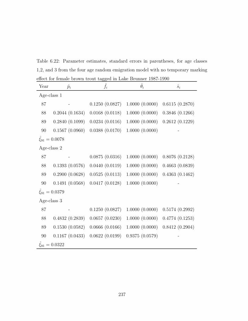
Table 6.22: Parameter estimates, standard errors in parentheses, for age classes
1,2, and 3 from the four age random emigration model with no temporary marking
effect for female brown trout tagged in Lake Brunner 1987-1990
Year pi fi θi si
Age-class 1
87 - 0.1250 (0.0827) 1.0000 (0.0000) 0.6115 (0.2870)
88 0.2044 (0.1634) 0.0168 (0.0118) 1.0000 (0.0000) 0.3846 (0.1266)
89 0.2840 (0.1099) 0.0234 (0.0116) 1.0000 (0.0000) 0.2612 (0.1229)
90 0.1567 (0.0960) 0.0388 (0.0170) 1.0000 (0.0000) -
ξ91 = 0.0078
Age-class 2
87 - 0.0875 (0.0316) 1.0000 (0.0000) 0.8076 (0.2128)
88 0.1393 (0.0576) 0.0440 (0.0119) 1.0000 (0.0000) 0.4663 (0.0839)
89 0.2900 (0.0628) 0.0525 (0.0113) 1.0000 (0.0000) 0.4363 (0.1462)
90 0.1491 (0.0568) 0.0417 (0.0128) 1.0000 (0.0000) -
ξ91 = 0.0379
Age-class 3
87 - 0.1250 (0.0827) 1.0000 (0.0000) 0.5174 (0.2992)
88 0.4832 (0.2839) 0.0657 (0.0230) 1.0000 (0.0000) 0.4774 (0.1253)
89 0.1530 (0.0582) 0.0666 (0.0166) 1.0000 (0.0000) 0.8412 (0.2904)
90 0.1167 (0.0433) 0.0622 (0.0199) 0.9375 (0.0579) -
ξ91 = 0.0322
237

Table 6.23: Results of contingency table tests for age- dependence and temporary
marking effect. Model 1: no age-dependence and no marking effect; Model 2a
marking effect but no age-dependence; Model 2b: age-dependence but no marking
effect; Model 3: age-dependence and marking effect.
Null model Alternative model
Model 2a Model 2b Model 3
Model 1 χ28 = 5.03, p = 0.754 χ2
22 = 47.03, p = 0.002 -
Model 2a - - χ224 = 50.12, p = 0.001
Model2b - - χ210 = 12.76, p = 0.240
dependence but no marking effect) appears to provide an adequate fit (χ23 = 6.01,
p = 0.11), hence the more general model must also provide an adequate fit.
238

Table 6.24: Reduced m-array with temporary marking effect for age-class 0 male
brown trout tagged in Lake Brunner 1987 - 1990.
Retrapped Captured by angler
Cohort j = 88 89 90 j = 87 88 89 90 91
Age 0, mark class 0 - released following capture
at spawning.
87 0 0 0 1 1 0 0 0
88 1 0 0 1 0 0
89 4 2 0 1
90 3 0
Released following capture
by anglers.
87 0 0 0 0 0 0 0
88 0 0 0 0 0
89 0 0 0
90 0
239

Table 6.25: Reduced m-array with temporary marking effect for age-class 1 male
brown trout tagged in Lake Brunner 1987 - 1990.
Retrapped Captured by angler
Cohort j = 88 89 90 j = 87 88 89 90 91
Age 1, mark class 0 - released following capture
at spawning.
87 2 3 2 2 1 0 0 0
88 2 4 2 4 2 0
89 5 6 2 0
90 8 2
Released following capture
by anglers.
87 0 0 0 0 0 0 0
88 0 0 0 0 0
89 0 0 0
90 0
Age 1, mark class 1 - released following capture
at spawning.
87 - - - - - - - -
88 0 0 0 0 0 0
89 0 0 0 0
90 0 1
Released following capture
by anglers.
87 - - - - - - - -
88 0 0 0 0 0
89 0 0 0
90 0
240

Table 6.26: Reduced m-array with temporary marking effect for age-class 2 male
brown trout tagged in Lake Brunner 1987 - 1990.
Retrapped Captured by angler
Cohort j = 88 89 90 j = 87 88 89 90 91
Age 2, mark class 0 - released following capture
at spawning.
87 4 12 2 14 2 0 0 0
88 6 5 11 3 1 0
89 7 21 8 0
90 15 11
Released following capture
by anglers.
87 0 0 0 0 0 0 0 0
88 0 0 0 0 0 0
89 0 0 0 0
80 0 3
Age 2, mark class 1 - released following capture
at spawning.
87 - - - - - - - -
88 0 1 0 0 0 0
89 0 0 0 0
90 1 1
Released following capture
by anglers.
87 - - - - - - - -
88 0 0 0 0 0
89 0 0
90 0
241

Table 6.27: Reduced m-array with temporary marking effect for age-class 3 male
brown trout tagged in Lake Brunner 1987 - 1990.
Retrapped Captured by angler
Cohort j = 88 89 90 j = 87 88 89 90 91
Age 3, mark class 0 - released following capture
at spawning.
87 4 4 1 7 1 1 0 0
88 1 0 2 1 0 0
89 4 9 2 0
90 5 11
Released following capture
by anglers.
87 0 0 0 0 0 0 0
88 0 0 0 0 0
89 0 0
90 1
Age 3, mark class 1 - released following capture
at spawning.
87 - - - - - - - -
88 0 0 1 1 0 0
89 3 1 0 1
90 4 2
Released following capture
by anglers.
87 - - - - - - - -
88 0 0 0 0 0 0
89 0 0 0 0
90 0 0
242

Table 6.28: Summary statistics for age-class 0 male brown trout tagged in spawning
tributaries of Lake Brunner 1987-1990 and observed by anglers 1987-1991.
year Ni Ri,1 ni Ri,2 Ci Oi Zi Ti ri Li
Age-class 0, mark class 0
87 6 2 0 0 0 1 0 0 2 1
88 31 2 0 0 0 0 1 1 2 0
89 67 7 0 0 1 2 1 2 7 2
90 56 3 0 0 4 3 1 5 3 3
Table 6.29: Summary statistics for age-class 1 male brown trout tagged in spawning
tributaries of Lake Brunner 1987-1990 and observed by anglers 1987-1991.
year Ni Ri,1 ni Ri,2 Ci Oi Zi Ti ri Li
Age-class 1, mark class 0
87 48 10 0 0 0 2 0 0 10 2
88 108 14 0 0 2 2 6 8 14 2
89 114 13 0 0 2 6 10 12 13 6
90 86 10 2 0 5 8 2 7 10 6
Age-class 1, mark class 1
87 0 0 0 0 0 0 0 0 0 0
88 0 0 0 0 0 1 0 0 1 1
89 1 0 0 0 0 1 0 0 1 1
90 4 1 0 0 0 0 0 0 2 0
243

Table 6.30: Summary statistics for age-class 2 male brown trout tagged in spawning
tributaries of Lake Brunner 1987-1990 and observed by anglers 1987-1991.
year Ni Ri,1 ni Ri,2 Ci Oi Zi Ti ri Li
Age-class 2, mark class 0
87 119 34 1 0 0 14 0 0 34 13
88 205 26 1 0 4 11 16 20 26 10
89 303 36 1 0 6 21 9 15 36 20
90 256 26 7 3 7 15 8 15 26 8
Age-class 2, mark class 1
87 0 0 0 0 0 0 0 0 0 0
88 2 1 0 0 0 1 0 0 7 1
89 2 0 1 0 3 4 3 6 10 3
90 5 2 0 0 4 3 2 6 4 3
Table 6.31: Summary statistics for age-class 3 male brown trout tagged in spawning
tributaries of Lake Brunner 1987-1990 and observed by anglers 1987-1991.
year Ni Ri,1 ni Ri,2 Ci Oi Zi Ti ri Li
Age-class 3, mark class 0
87 61 18 0 0 0 7 0 0 18 7
88 49 4 0 0 4 2 7 11 4 2
89 86 15 3 0 1 9 1 2 15 6
90 80 16 3 1 4 5 2 6 16 2
Age-class 3, mark class 1
87 0 0 0 0 0 0 0 0 0 0
88 8 2 0 0 0 4 0 0 25 4
89 26 5 1 0 16 7 5 21 23 6
90 29 6 3 0 14 17 2 16 20 14
244

Table 6.32: Parameter estimates for age-class 0 males under the 4-age model with
temporary marking effect under random emigration fitted to the male data.
Year pi fi θi Si ξi
Age-class 0, mark class 0
87 - 0.1667 1.0000 - -
88 - 0.0000 1.0000 - -
89 0.0000 0.0299 1.0000 0.1194 -
90 0.5000 0.0536 1.0000 - -
91 - - - - 0.0000
245

Table 6.33: Parameter estimates for age-class 1 males under the 4-age model with
temporary marking effect under random emigration fitted to the male data.
Year pi fi θi Si ξi
Age-class 1, mark class 0
87 - 0.0417 1.0000 0.2917 -
88 0.1429 0.0185 1.0000 - -
89 0.0000 0.0526 1.0000 0.0877 -
90 0.5000 0.0930 1.0000 - -
91 - - - - 0.0233
Age-class 1, mark class 1
87 - - - - -
88 - - 1.0000 - -
89 - 0.0000 1.0000 0.0000 -
90 - 0.0000 1.0000 - -
91 - - - - 0.2500
246

Table 6.34: Parameter estimates for age-class 2 males under the 4-age model with
temporary marking effect under random emigration fitted to the male data.
Year pi fi θi Si ξi
Age-class 2, mark class 0
87 - 0.1176 1.0000 0.5714 -
88 0.0588 0.0537 1.0000 0.2576 -
89 0.1136 0.0693 1.0000 0.1507 -
90 0.1533 0.0586 0.7857 - -
91 - - - - 0.0430
Age-class 2, mark class 1
87 - - - - -
88 - 0.0714 1.0000 1.3286 -
89 0.1613 0.0000 1.0000 0.0000 -
90 0.2927 0.3000 1.0000 - -
91 - - - - 0.1000
There was evidence of a temporary marking effect (p < 0.025) but only weak
(0.05 < p < 0.1 evidence of age-dependence (Table 6.36).
The age-independent random emigration model with temporary marking ef-
fect was fitted to the male data set. Tests for a marking effect in the capture
probabilities, survival rates, and unconditional observation probabilities indicated
that the temporary marking effect was manifest through the capture probabilities
(χ22 = 12.47, p = .002) but not the survival rates (χ2
2 = 0.85, p = .655). There was
weak evidence of a temporary marking effect in the fi’s (χ3 = 6.48, p = .090). There
were insufficient data to test for a marking effect in the θi’s. Parameter estimates
for the age-independent random emigration model with temporary trap response
in just the capture probabilities is given in Table 6.37. This model provides an
adequate fit to the data χ211 = 14.05, p = 0.232.
247

Table 6.35: Parameter estimates for age-class 3 males under the 4-age model with
temporary marking effect under random emigration fitted to the male data.
Year pi fi θi Si ξi
Age-class 3, mark class 0
87 - 0.1148 1.0000 0.5246 -
88 0.1250 0.0408 1.0000 0.1265 -
89 0.1613 0.1047 1.0000 0.1589 -
90 0.2927 0.0625 0.9167 - -
91 - - - - 0.1375
Age-class 3, mark class 1
87 - - - - -
88 - 0.0400 1.0000 0.4200 -
89 0.3810 0.0585 1.0000 0.1979 -
90 0.5915 0.1759 1.0000 - -
91 - - - - 0.0310
Table 6.36: Results of contingency table tests for age- dependence and temporary
marking effect for males. Model 1: no age- dependence and no marking effect;
Model 2a marking effect but no age-dependence; Model 2b: age-dependence but no
marking effect; Model 3: age-dependence and marking effect.
Null model Alternative model
Model 2a Model 2b Model 3
Model 1 χ27 = 24.85, p = 0.001 χ2
26 = 37.96, p = 0.061 -
Model 2a - - χ226 = 35.97, p = 0.092
Model2b - - χ28 = 17.91, p = 0.021
248

Table 6.37: Parameter estimates, standard errors in parentheses, for the age-
independent random emigration model with temporary marking effect in capture
probabilities for male brown trout tagged in Lake Brunner 1987-1990
Year pi fi θi si
Trap-class 0
87 - 0.1026 (0.0198) 1.0000 (0.0000) 0.7119 (0.1740)
88 0.0600 (0.0234) 0.0375 (0.0085) 1.0000 (0.0000) 0.3561 (0.0834)
89 0.0720 (0.0273) 0.0650 (0.0095) 1.0000 (0.0000) 0.2586 (0.0676)
90 0.1363 (0.0446) 0.0753 (0.0115) 0.8363 (0.0662) -
ξ91 = 0.0496(0.0099)
Trap-class 1
87 -
88 -
89 0.3146 (0.0975)
90 0.3446 (0.1178)
ξ91 = 0.0310(0.0146)
249

6.3 Discussion
Overall, the age-dependent random emigration model with no temporary marking
effect seems to provide the best representation of the data set for females. In
contrast, the results for males indicate that a model with a temporary marking
effect but no age-dependence best fits the data. However an alternative explanation
that should be examined is that there is Markovian movement of males between
spawnings.
The implication of the random emigration model with temporary marking ef-
fect is that males avoid the trap in the second year following initial capture but not
in subsequent years. Moreover, behaviour is not altered by subsequent encounters
with the trap. Given that the animals are only marked on their first encounter
with the trap, and that marking involves application of a plastic tag through the
flesh via a needle the first trapping occasion does provide the fish with a potentially
unpleasant experience. Thus a temporary marking effect induced at the first cap-
ture occasion provides a plausible explanation for the observed data. A weakness
with this explanation is that since both sexes are treated alike, there should be a
similar response for females, however there was no evidence of a similar response
for females. Indeed, if the temporary marking effect model is correct, then there
needs to be some explanation for the lack of evidence of a temporary marking effect
for females.
In the absence of a clear biological explanation for this result a reasonable
conclusion for males is that there is some process affecting capture probabilities
but it is unclear whether this is a consequence of animal movement patterns or
whether the underlying behaviour is induced by the experiment.
The biological interpretation of the Markov emigration model is that brown
trout spawning in year i are less likely to spawn in year i+ 1 than those trout that
do not spawn in year i. Again, if this is the correct model we need a reasonable
explanation as to why this is the case for males but not for females. Given the
different roles of males and females in the spawning process such an asymmetry
250

in spawning behaviour between the sexes may be a reasonable explanation for
the observed results. If the Markov movement model is correct, and if in fact
males and females are utilizing different reproductive strategies, then there are
some interesting possibilities. For example, if we denote spawning in year i, not in
i + 1 and then spawning in year i + 2 as the 101 strategy and spawning in each
of the years i, i + 1, i + 2 as the 111 strategy, then the 101 strategy provides a
longer recuperation period between spawnings with a potential benefit in terms of
resources that can be put into each reproductive effort, but it involves a greater
exposure to mortality factors between spawnings. Thus depending on values for
key parameters a 101 strategy may lead to greater expected lifetime reproductive
output than the 111 strategy.
A satisfactory way to resolve this question may be to carry out some sort of ex-
periment designed to discriminate between the different possibilities. One approach
would be to obtain observations of marked fish in the spawning stream above the
trap following trapping. If there is no marking effect, then of those fish marked
before i observed in the spawning stream after trapping between i and i + 1, the
proportion that were also trapped at i should not depend on whether the fish were
first marked at i + 1.
251

252

Chapter 7
Discussion
7.1 Benefits of the New Models and Implications
for Existing Methods
The extension of the Jolly-Seber model to incorporate observations of animals be-
tween capture periods unites mark-recapture, mark-resight and tag-recovery models
in a common framework and allows simultaneous estimation of parameters when
data are gathered in all three ways. An important advantage is that all data can
be used in an efficient manner with potentially large reductions in variances of key
parameter estimates such as survival rates. We considered gains in precision only
under random emigration. Under permanent emigration, the gains may be even
greater due to the fact that once an animal has emigrated, it can never be available
for recapture again (K. P. Burnham, pers. comm.). Under random emigration this
loss of animals need only be temporary.
In addition to gains in precision, the inclusion of ancillary observations allows
separation of the parameters St−1 and pt which in the Jolly-Seber model are con-
founded. It also allows separate fitting of the model under different assumptions
about movement of animals in and out of the study area. In addition we have shown
how the assumption of a negligible sampling period can be relaxed in a tag-resight
study, and we have shown how to include losses on observation.
253

The introduction of ancillary observations into the analysis and the differing
means of representing the movement of animals into and out of the component of
the population that is at risk of capture leads to a very large class of models that
can be fitted to any given data set. As illustrated by the west coast trout tagging
example, the models to be fitted may have a very large number of parameters and
the data set needed to fit the fullest models may be sparse. While this proliferation
of potential models may appear to cause some model fitting and selection difficulties,
it is generally better to have a large set of potential models to choose from than a
restricted class of models.
The focus of our treatment has been the estimation of capture probabilities,
survival rates, and observation rates. As in the Jolly-Seber model estimation of
population size using ancillary observations in addition to recaptures involves first
specifying a model for captures of unmarked animals. The usual assumption, (i.e.
as in the Jolly-Seber model) is that unmarked and marked animals are captured at
i with the same probability pi. Under the assumption of permanent emigration the
expected number of animals captured at i in the one-age model without marking
effect is given by
E[ni] = Ni−1Si−1Fi−1pi +Bi−1pi
= Nipi ,
where Ni is the total number of animals in the at-risk-of-capture segment of the
population at i and Bi is the number of new animals recruited into the population
between i− 1 and i who are in the at risk of capture segment of the population at
i. The obvious population size estimator under permanent emigration is then the
Jolly-Seber MLE
Ni =ni
pi
. (7.1)
Under Markov emigration we must also specify the probability that the recruits
are at risk of capture which we denote F ′
i . Hence
E[ni] = Ni−1,ASi−1ψi−1,1,1pi +Ni−1,NSi−1ψi−1,2,1pi +Bi−1F′
ipi
= Ni,Api ,
254

where Ni,A is the total number of animals at risk of capture at i and Ni,N the total
number not at risk of capture at i. Hence (7.1) will be an estimate of the size
of Ni,A. To obtain MLE’s of population size under either permanent or Markov
emigration a component corresponding to unmarked animals can be included in
the likelihood as described in Section 1.3.3 for the Jolly-Seber model.
Under random emigration
E[ni] = Ni−1,ASi−1Fi−1pi +Ni−1,NSi−1Fi−1pi +Bi−1F′
ipi .
Unlike the permanent emigration or Markov emigration models, under random
emigration we cannot estimate pi, just the product Fi−1pi. Hence if Bi−1 does
not equal zero, we cannot estimate the size of the population (either total or at
risk of capture) without a further restriction on F ′
i . For example if we assume
F ′
i = Fi then the Jolly-Seber MLE is an estimate of the total population size at
i, however this assumption is unreasonable unless animals are recruited exactly
at i. Thus, under random emigration we do not appear to be able to estimate
population size without restrictive assumptions about the movement of recruits
or without additional information. For example, under Pollock’s (1981) “robust”
design, population size is estimated using the closed population models described
in section 1.1. Hence population size can be estimated regardless of the assumption
about movement of animals between primary capture periods (Nichols et al. unpubl.
manuscr.)
The situation that we have described applies equally to the Jolly-Seber model
(i.e. without ancillary observations). This is even more unsatisfying as without an-
cillary observations the two movement assumptions lead to identical expected recap-
tures and we cannot distinguish between the models. Moreover, the goodness-of-fit
statistics for the Jolly-Seber model test only the fit of the model to the recaptures
of marked animals. Thus we have two equally valid models for marked animals,
no means of distinguishing between them, and we only have a valid population
size estimator under permanent emigration. In addition, in the Jolly-Seber model
we are unable to determine whether the Jolly-Seber survival rate estimator φi is
255

a true survival rate Si (i.e random emigration) or SiFi, the joint probability that
an animal has survived and not emigrated (i.e permanent emigration). This result
reinforces the importance of obtaining additional information that allows separate
modelling of the different types of emigration.
7.2 Implication for the Design of New Studies
There are many situations in which mark-recapture data with ancillary observations
may arise. The “ancillary” observations may in fact be the focus of the recapture
effort as in the case of a tag-resight or a tag-return study. In such a study the
new aspect of the analysis introduced by the models presented in this thesis is the
inclusion of the live-recaptures as well as relaxation of the assumption that resight-
ings are carried out over a negligible time period. As methods of data acquisition
become more sophisticated (e.g. the use of passive integrated transponder tags or
satellite telemetry) it may become increasingly easy to obtain observations on ani-
mals between capture periods and we may see increasing collection of resight data
to be used in conjunction with recapture data.
In many studies the focus of the study may indeed be a live-recapture experiment
but where sightings of marked animals are reported by members of the public. In
the situation envisaged by Jolly (1965) the experimenter may deliberately seek
such ancillary sightings. An interesting point arises in the situation considered
by Jolly (1965) if the resources put into observations of animals between capture
periods compete with the resources available for live-recapture and marking. An
interesting follow-up study would be to consider the optimal allocation of resources
from the point of view of estimation of S1,...,St−2, say. In the case of St−1 the design
with ancillary observations is superior as an estimate is not otherwise possible.
The inclusion of resightings in the model and the associated parameters fi and θi
raise the possibility of studies where these parameters are of specific interest. There
are many examples in fisheries and wildlife management where animal counts with
unknown observation probabilities are used as indices of abundance (i.e. as indi-
256

cators of population change). A feature of all such trend monitoring methods is
that they assume that the observation probabilities remain constant through time,
and possibly space, or that they can be modelled in some simple way. In a case
where the index method yields observations of marked animals an interesting anal-
ysis would be to explicitly estimate time and geographic effects on the observation
probabilities.
7.3 Future Research
7.3.1 Direct modelling of capture histories
In this thesis, the primary effort has been in developing a model under random
emigration after first summarizing the data using an m-array. As is needed for the
permanent emigration and Markov emigration model, an alternative is to model
the individual capture histories directly. An advantage to this approach is that it
allows the model to be generalized to include individual covariates.
It has also been pointed out (K. P. Burnham pers. comm.) that the goodness
of fit tests reported in this thesis will not be fully efficient as there is some infor-
mation lost in summarizing the capture history data using the m-array. Each of
the release cohorts in the m-array (i.e. the Ci,k’s) can be partitioned according to
the time at which the animal was first captured. Utilizing this partitioning into
“subcohorts”, contingency tables contributing information on goodness of fit of the
random emigration model can be constructed leading to a test similar in form to
TEST 3 of Burnham et al. (1987:74-77). Under permanent and Markov emigra-
tion information needed for parameter estimation is lost in the Mi,j,2,k summary
of recaptures/resightings for animals last released following observation. Therefore
the TEST 3 component will be sensitive to departures from the random emigration
model caused by Markovian movement.
257

7.3.2 Alternative handling effect models
The marking effect models of section 4.3 are appropriate in the case when capture
lowers the probability of capture or observation in the period immediately following
initial capture. However, it is possible to envisage a situation where a similar effect
occurs after any capture, not just the first one, but as in the temporary marking
effect model, we may be prepared to assume this effect “wears off” after one time
period. Under the Jolly-Seber model Burnham et al. (1987:218-221) show that
a handling effect on survival rates that occurs at each capture leads to a model
structure that has an MSS identical to that of the Jolly-Seber model. Therefore
the handling effect model cannot be distinguished from the Jolly-Seber model. The
difficulty arises when all information following release is provided by recaptures,
because recaptures neccessarily involve handling.
It is possible that where some information comes from resightings in addition to
recaptures identifiable handling effects models might be constructed. For simplicity,
we just consider the case of a single age-class. If we let class 0 animals at time i be
those animals captured at i, and class 1 those animals not captured at i, and if we
write the probability structure for the model out, we find that it leads to an identical
structure to the model of section 4.3, but where there are no C(1)i,1 animals since all
animals captured at i are released in a C(0)i,1 cohort. Because the C
(1)i,1 are required to
estimate λ(1)i,1 this model will not be fully identifiable (i.e. the dimension of the MSS
is lower than the dimension of the parameter space), and some constraints will be
required. In particular we are unable to estimate the δ(1)i . In certain cases it may
be reasonable to assume that the handling effects do not influence the probability
an animal is observed. This allows us to make the constraint δ(1)i = δ
(0)i and the
model may become identifiable.
We may be able to further generalize this model and allow separate tagging and
handling effects. Thus an animal which is both handled and tagged at i can have
different survival and or capture and or observation probabilities than animals which
are just handled, or not handled at all. In our brown trout example considered in
Chapter 6 the fish received a physical insult at tagging but not on later recaptures.
258

Thus, the response to initial capture might be stronger than the response to later
captures.
7.3.3 General multi-strata movement model
In Chapter 4 we discussed special cases of multi-strata models where movement was
highly structured in that it was deterministic and one-way. Schwarz et al. (1991)
and Brownie et al. (1993) have demonstrated how the Jolly-Seber model and tag-
return models can be generalized to permit two-way movement between strata.
Schwarz et al (1993) assumed that movement could be described by a Markov
chain, and Brownie et al. (1993) generalized this to allow “memory”, where the
dependence extends for more than one time period.
Except in the case of joint live-recovery and tag-return models the theory we
have described in Chapter 3 and the current Chapter does not appear to fully gen-
eralize to the multi-strata case with Markovian movement between strata because
of the re-release of animals following observation. In the case of tag-return models
the animals are not re-released, simplifying the problem.
The difficulty arises because in the general multi-strata Jolly-Seber and tag-
return models stratification is defined with respect to the capture process. Thus
we model the manner in which animals are in stratum k at capture time i, and
at stratum l at capture time i + 1 and are able to avoid making an assumption
about how the animals move between time periods. This movement may follow
some clear pattern or it may be chaotic. It does not matter as far as the model is
concerned. To make use of observations between i and i+1 in a manner analogous
to the single-stratum case we need to determine the probability that an animal
alive at time i in location k is alive at time i + 1 and in location l given that
it was observed between times i and i + 1 at location m (or even several different
locations). In the unconstrained case we make no assumption about the mechanism
by which animals at location k at i move through location m some time between
i and i + 1, then appear at location l at time i + 1. In the absence of simplifying
assumptions, we require additional parameters to describe this movement and the
259

model becomes over-parameterized. These parameters are required in order to link
the strata occupied at time of observation in i, i+ 1 to the strata occupied at time
i and i + 1.
A useful solution might be to completely ignore the stratum occupied on obser-
vation. In such a case we utilize the fact that the animals were observed somewhere
to contribute information on the survival process. To illustrate the basic form of
this model we consider a one-age model in the absence of a marking effect with
t years of capture and observation. For a study with s strata we generalize the
notation of Chapter 3 so that:
Statistics
Mi,j,k,1 is an s x s matrix with g, hth element Mi,j,k,1,g,h the number of
animals last released at time i following encounter by method k (k =
1, 2) in stratum g that are next encountered by capture at j in stratum
h.
M i,j,k,1 is an s x 1 vector with gth element Mi,j,k,2,g the number of
animals last released at time i following encounter by method k (k =
1, 2), and that were last captured in stratum g, that are next encountered
by observation between j and j + 1 in any stratum.
260

Parameters
Si = the sxs matrix with g, hth element Si,g,h, the probability an animal
alive and in stratum g at time i is alive and in stratum h at i + 1.
θi = an sx1 vector with gth element θi,g, the probability an animal alive
and in stratum g at time i is not observed between i and i + 1 given
that it is alive at i+ 1.
fi= an sx1 vector with gth element fi,g, the probability an animal alive
and in stratum g at time i is observed between i and i + 1.
pi the sxs matrix with g, hth element pi,g,h, the probability an animal
in stratum g at i− 1 and alive at i is captured in stratum h at i.
Ψi = the sxsmatrix with g, hth element ψi,g,h, the probability an animal
alive and in stratum g at time i is in stratum h given it is also alive at
i+ 1.
ρi
= an sx1 vector with gth element ρi,g, the probability an animal
observed in stratum g at time i is released.
Note in particular that the elements of the vector M i,j,k,1 are indexed by where the
animals were last captured, not the stratum in which they were observed between
i and i + 1. In this way the strata are identified only by capture location.
Let D(x) be the diagonal matrix with j, jth element given by the jth element
of the vector x, and A · B represent element-by-element multiplication of the con-
formable matrices A and B and the matrix 1−A be the matrix with i, jth element
given by 1 − Ai,j. We also define the working parameter matrices
qi = 1 − pi
Φi = D(θi)Si · Ψi
and
∆i = D−1(fi)D−1(ρ
i)D(1 − θi)D
−1(θi) .
261

To develop the probability structure of the model we first arrange the data in
the form of the multivariate m-array illustrated in Table 7.1.
Table 7.1: Multivariate reduced m-array for a mark-recapture study beginning at
time 1 with t capture periods and ancillary observations of marked animals obtained
during the interval 1, t+ 1.
Cohort Next encountered by capture Next encountered by observation
j = 2 3 ... t j = 1 2 ... t − 1 t
Ci, -last released following capture
i=1 M1,2,1,1 M1,3,1,1 ... M1,t,1,1 M1,1,1,2 M1,2,1,2 ... M1,t−1,1,2 M1,t,1,2
2 M2,3,1,1 ... M2,t,1,1 M2,2,1,2 ... M2,t−1,1,2 M2,t,1,2
. . . . . . . . .
t − 1 ... Mt−1,t,1,1 ... M t−1,t−1,1,2 M t−1,t,1,2
t ... M t,t,1,2
Ci, - last released following observation
i=1 M1,2,2,1 M1,3,2,1 ... M1,t,2,1 M1,2,2,2 ... M1,t−1,2,2 M1,t,2,2
2 M2,3,2,1 ... M2,t,2,1 ... M2,t−1,2,2 M2,t,2,2
. . . . . . . . .
t − 1 ... Mt−1,t,2,1 ... M t−1,t,2,2
If we let Πi,j,m,n = the multionomial cell probability for the Mi,j,m,n conditional
on the releases then the corresponding multivariate “cell” probabilities are given
by
Πi,j,1,1 = Φiqi+1Φi+1qi+2 · · ·Φj−2qj−1Φj−1pj ,
Πi,j,2,1 = ∆iΠi,j,1,1 ,
Πi,j,1,2 = D(fj)Φiqi+1Φi+1qi+2 · · · Φj−2qj−1Φj−1qj ,
Πi,j,2,2 = D(fj∆i {Φiqi+1Φi+1qi+2 · · ·Φj−2qj−1Φj−1qj} .
262

The final multivariate “cell” vector corresponding to animals that were never cap-
tured or seen again following release has probability
1 −
t∑
j=i+1
Πi,j,1,1 +t∑
j=i
Πi,j,1,2
for animals last released following capture and
1 −
t∑
j=i+1
Πi,j,2,1 +t∑
j=i+1
Πi,j,2,2
for animals last released following observation.
This representation of a multi-state mark-recapture model with captures aug-
mented by observations between capture periods represents a generalization of
model JMV described by Brownie et al. (1993). Numerical procedures can be used
to find MLE’s subject to appropriate identifiability constraints similar to those im-
posed by Schwarz et al. (1993) and Brownie et al. (1993). As an alternative to
MLE’s, we might be able to find moment estimators that are matrix analogues of
the Chapter 3 estimators as reported by Brownie et al. (1993) for their model JMV.
An alternative to the above approach of ignoring stratum occupied on obser-
vation is to impose some constraint on the movement process as we have done in
the age-dependent and temporary marking effect models. Because of the potential
complexity of the models it is likely that in different experimental situations dif-
ferent constraints on movement will be relevant. Thus a general model relevant to
most experimental situations will be unlikely to exist.
Possible constraints on movement may include modelling movement via diffusion
models. In such a model the exact time at which the animal was observed between i
and i+1 would be relevant, and we would make use of multiple observations between
capture occasions. In some cases the problem may be simplified by movement
occurring at some exact time in the interval i, i + 1 which is common to all such
intervals. For example in migratory species there may be a clearly defined pattern
of movement that can be exploited in simplifying the model. In other cases the
observations may be gathered over a short period at the same time in each between-
capture interval, thus we could have one set of movement parameters for the two
263

sets of movements between capture periods. Regardless of the modelling approach
we also need to consider how we model the process by which animals are at risk
of capture within a stratum. For example, animals may be at risk of capture
throughout each stratum or they may be at risk of capture only in a portion of the
stratum.
7.3.4 Models with different resighting assumptions
In the models discussed in this thesis, we assume that animals are available for
resighting throughout their geographic range, but otherwise there are no restrictions
on the sampling process. An obvious restriction that can be incorporated in any
new models is where resighting occur over a restricted range. If resightings can
only occur over the same area where animals are at risk of capture then we are
in the situation faced by the Jolly-Seber model where we can have either random
or permanent emigration, but we are unable to tell which. If we have permanent
emigration, then the survival rate parameter would need to be reinterpreted as the
product FiSi. Note that if we have stationary Markov emigration, we may still be
able to fit the model.
In the intermediate case, where resightings occur over a larger but not all-
encompassing range, we may be able to fit all three models, but the parameter
definitions would require appropriate redefinition. For example, if the movement
in and out of the resighting area were random then we would still have Si as a true
survival rate, but fi and θi would be redefined as joint movement and resighting
probabilities. If movement from the resighting area was permanent, then Si would
require redefinition as the probability the animal remains in the resighting area
between i and i + 1 and survives.
In some studies it may be possible to determine the at-risk-of-capture status for
an animal at time i for animals resighted between i and i + 1. If this information
is available, then we have a special case of the general multi-strata problem but
where recapture can only occur in the at-risk-of-capture stratum. The advantage
of a model developed to allow this possibility would be that discrimination between
264

the three types of movement model discussed in this thesis would likely be improved.
Reliable determination of whether an animal resighted in i, i+1 was also at risk
of capture may be difficult for two reasons. First, if the period between captures is
long, there may be considerable movement of animals with respect to the trapping
site making identification of the position of the animal at i difficult. Second, the
definition of the population of animals at risk of capture in a mark recapture study is
often vague. All we know is that it is the animals that were vulnerable to our capture
technique at the time of captures. The area within which these animals occur may
be poorly delimited. One possible exception might be where it is breeding animals
that are at risk of capture, and that during the interval i, i + 1 we can determine
the breeding status of an animal at time i.
7.3.5 Investigations concerning underlying assumptions
Ultimately, the usefulness of any model(s) depends on the extent to which key as-
sumptions are violated As noted by McCullagh and Nelder (1989) “..all models are
wrong; some though, are better than others...”. In Chapter 5 we briefly considered
the extent to which heterogeneous capture probabilities might bias estimates pro-
duced for the models described in this thesis. Because with real data some, and
possibly all, the assumptions of the model may be violated to a certain extent it
is important to consider the effect of these violation on the estimators. Further
investigations of this nature would be of interest.
A particularly important assumption is that animals do not lose their tags.
The effect of tag loss on the Jolly-Seber and tag-return estimators is well known
(Arnason and Mills 1981, Nelson et a. 1980, Pollock 1981a). Intuitively, the loss
of tags acts in a similar manner to mortality and in the absence of additional
information tag loss parameters will be confounded with survival rate parameters.
In many studies incorporating resightings, the animals are marked with large, easy
to read tags. In some studies these tags are known to have a non-negligible rate
of loss, and animals are also marked with a smaller, permanent tag that can only
be read when the animal is recaptured. Such double tagging permits estimation of
265

the rates of tag loss. If the rate of tag loss depends only on i and not on the time
since tagging, then estimation in such double tagging schemes is straight forward
(Arnason and Mills 1981, Pollock 1981). If Si is the survival rate computed using
the mark-recapture or mark-resight model and if θi is the tag loss rate between i
and i+ 1 then the corrected survival rate estimator is simply
Sci =
Si
θi
.
In many situations it is not reasonable to assume that the rate of tag loss depends
only on i. Samuel et al. (1990) (Canada geese) and Nichols et al. (1992) (tundra
swan) found evidence that the annual neckband retention probability decreased
with increasing time since application.
Kremers (1988) and Nichols et al. (1992) showed that in a double tagging study
where animals are recaptured as well as resighted it is possible to develop a joint
likelihood incorporating both recapture and resighting data. The model of Kremers
requires the restrictive assumption that one of the tags is permanent and that the
period between recaptures and resighting is negligible. Also, the models of Kremers
(1988) use only the final observation of the animal. The model of Nichols et al.
(1992) utilized recapture data only as a source of information about tag-retention
rate and not recapture and survival probabilities and ignored intermediate captures.
However, an important advantage of the models of Nichols et al. (1992) is that they
do not assume that one tag is permanent. An important area of future research
might be to consider the extension of the models discussed in this thesis to allow
for double tagging. This may lead to the development of more efficient models that
make full use of recapture and observation data and permit simultaneous estimation
of tag-retention and survival probabilities.
7.4 Concluding Remarks
By including observations on marked animals from different sources the experi-
menter has a potentially richer class of models from which to choose a suitable
266

model. Particularly important is the ability to distinguish between different possi-
ble types of emigration, provided at least one type of data includes observations on
animals from throughout their geographic range. Mark-recapture studies have for
the most part been based on one type of “recapture” data, and studies based on
more than one source of recapture data are unusual. We concur with Nichols and
Hines (1993) who recommended that the designs of resighting studies include ef-
forts to recapture animals. In addition we recommend that a similar effort to catch
marked animals is made in tag-recovery studies, and in live-recapture studies, that
an effort is made to obtain observations on animals throughout the range of the
study population. A particularly important issue is the allocation of resources to
the different aspects of the study. As noted by Nichols and Hines (1993), knowledge
of the relationship between effort and both recapture and observation probabilities
will allow consideration of the optimal allocation of resources in future studies.
Bibliography
Alho, J. M. 1990. Logistic regression in capture-recapture models. Biometrics
46:623-635.
Anderson, D. R. and K. P. Burnham. 1976. Population ecology of the mallard VI.
The effect of exploitation on survival. U.S. Fish and Wildlife Service Resource
Publication 128. 66pp.
Anderson, D. R., K. P. Burnham, and G. C. White. 1982. The effect of exploitation
on annual survival of mallard ducks: an ultrastructural model. Proceedings of
International Biometrics Conference 11:33-39.
Anderson, D. R., K. P. Burnham, and G. C. White. 1985. Problems in estimating
age-specific survival rates from recovery data of birds ringed as young. Journal
of Animal Ecology 54:89-98.
Anderson, D. R., K. P. Burnham, and G. C. White. 1994. AIC model selection in
267

overdispersed capture-recapture data. Ecology 75:1780 -1793.
Anderson, D. R. and R. T. Sterling. 1974. Population dynamics of molting pintail
drakes banded in south-central Saskatchewan. Journal of Wildlife Management
38:226-274.
Arnason, A. N. 1972. Parameter estimates from mark-recapture experiments on
two populations subject to migration and death. Researches in Population
Ecology 13:97-113.
Arnason, A. N. 1973. The estimation of population size, migration rates and sur-
vival in a stratified population. Researches in Population Ecology 15:1-8.
Arnason, A. N. and K. H. Mills. 1981. Bias and loss of precision due to tag loss
in Jolly-Seber estimates for mark-recapture experiments. Canadian Journal of
Fisheries and Aquatic Science 38:1077-1095.
Barker, R. J. 1992. Effect of heterogeneous survival on bird-banding model confi-
dence interval coverage rates. Journal of Wildlife Management 56:111-116.
Barker, R. J. and I. M. Buchanan. 1993. Estimating adult survival rates of New
Zealand black swans banded as immatures. Journal of Wildlife Management
57:549-555.
Barker, R. J., J. E. Hines, and J. D. Nichols. 1991. Effect of hunting on annual
survival of grey ducks in New Zealand. Journal of Wildlife Management 55:260-
265.
Becker, N. G. 1984. Estimating population size from capture-recapture experiments
in continuous time. Australian Journal of Statistics 26:1-7.
Bishop, Y. M. M., S. E. Fienberg, and P. W. Holland. 1975. Discrete Multivariate
Analysis. MIT Press, Cambridge, Massachusetts. 557pp.
Brownie, C. and D. S. Robson. 1976. Models allowing for age-dependent survival
rates for band-return data. Biometrics 32:305-323.
268

Brownie, C. and D. S. Robson. 1983. Estimation of time-specific survival rates from
tag-resighting samples: a generalization of the Jolly-Seber model. Biometrics
39:437-453.
Brownie, C., J. E. Hines, and J. D. Nichols. 1986. Constant-parameter capture-
recapture models. Biometrics 42:561-574.
Brownie, C., J. E. Hines, J. D. Nichols, K. H. Pollock, and J. B. Hestbeck. 1993.
Capture-recapture studies for multiple strata including non-Markovian transi-
tions. Biometrics 49:1173-1187.
Brownie, C., D. R. Anderson, K. P. Burnham, and D. S. Robson. 1985. Statistical
inference from band recovery data - a handbook. U.S. Fish and Wildlife Service
Resource Publication 156. 305pp.
Buckland, S. T. 1980. A modified analysis of the Jolly-Seber capture-recapture
model. Biometrics 36:419-435.
Buckland, S. T. 1984. Monte Carlo confidence intervals. Biometrics 40:81-817.
Burnham, K. P. 1991. On a unified theory for release resampling of animal pop-
ulations. pp 11-35 in M. T. Chao and P. E. Cheng (eds.). Proceedings of the
1990 Taipei Symposium in Statistics. Institute of Statistical Science, Academia
Sinica. Taipei, Taiwan, R. O. C.
Burnham, K. P. 1993. A theory for combined analysis of ring recovery and recapture
data. pp 199-213 in J.-D. Lebreton and P. North (eds). Marked individuals in
bird population studies. Birkhauser Verlag, Basel.
Burnham, K. P. and D. R. Anderson. 1979. The composite dynamic method as
evidence for age-specific waterfowl mortality. Journal of Wildlife Management
43:356-366.
Burnham, K. P. and D. R. Anderson. 1992. Data based selection of an appropriate
biological model: the key to modern data analysis. pp 16-30 in D. R. McCul-
269

lough and R. H. Barrett (eds.). Wildlife 2001: populations. Elsevier Applied
Science, London.
Burnham, K. P., D. R. Anderson, and G. C. White. 1994. Evaluation of the
Kullback-Leibler discrepancy for model selection in open population capture-
recapture models. Biometrical Journal 36:299-315.
Burnham, K. P., D. R. Anderson, and G. C. White. 1995b. Selection among open
population capture-recapture models when capture probabilities are heteroge-
neous. Journal of Applied Statistics 22:611-624.
Burnham, K. P., G. C. White, and D. R. Anderson. 1984. Estimating the effect
of hunting on annual survival rates of adult mallards. Journal of Wildlife
Management 48:350-361.
Burnham, K. P., G. C. White, and D. R. Anderson. 1995a. Model selection strategy
in the analysis of capture-recapture data. Biometrics 51:888-898.
Burnham, K. P., and W. S. Overton. 1978a. Estimation of the size of a closed
population when capture probabilities vary among animals. Biometrika 65:625-
633
Burnham, K. P., and W. S. Overton. 1978b. Robust estimation of population size
when capture probabilities vary among animals. Ecology 60:927-936.
Burnham, K. P., D. R. Anderson, G. C. White, C. Brownie, and K. H. Pollock.
1987. Design and analysis methods for fish survival experiments based on
release-recapture. American Fisheries Society Monograph 5. 437pp.
Burnham, K. P. and E. A. Rexstad. 1993. Modeling heterogeneity in survival rates
of banded waterfowl. Biometrics 49:1194-1208.
Carothers, A. D. 1973. the effects of unequal catchability on Jolly-Seber estimates.
Biometrics 29:79-100.
270

Catchpole, E. A. and B. J. T. Morgan. 1991. A note on Seber’s model for ring-
recovery data. Biometrika 78:917-919.
Chao, A. 1987. Estimating the population size for capture-recapture data with
unequal catchability. Biometrics 43:783-791.
Chao, A. 1989. Estimating population size for sparse data in capture-recapture
experiments. Biometrics 45:427-438.
Chao, A., S.-M. Lee, and S.-L. Jeng. 1992. Estimating population size for capture-
recapture data when capture probabilities vary by time and individual animal.
Biometrics 48:201-216.
Chapman, D. G. and C. O. Junge. 1956. The estimation of the size of a stratified
animal population. Annals of Mathematical Statistics 27:375-389.
Cormack, R. M. 1964. Estimates of survival from the sighting of marked animals.
Biometrika 51:429-438.
Cormack, R. M. 1968. The statistics of capture-recapture methods. Oceanography
and Marine Biology Annual Review 6:455-506.
Cormack, R. M. 1979. Models for mark-recapture. pp 217-255 in R. M. Cormack,
G. P. Patil, and D. S. Robson (eds.). Sampling Biological Populations. Inter-
national Cooperative Publishing House, Fairland, Maryland.
Cormack, R. M. 1981. Loglinear models for capture-recapture experiments on open
populations. pp 217-235 in R. W. Hiorns and D. Cooke (eds.). Mathematical
Theory of the Dynamics of Biological Populations. Academic Press, London.
Cormack, R. M. 1989. Log-linear models for capture-recapture. Biometrics 45:395-
413.
Cormack, R. M. 1993. Variances of mark-recapture estimates. Biometrics 49:1188-
1193.
271

Cormack, R. M. 1994. Unification of mark-recapture analyses by loglinear mod-
elling. pp 19-32 in D. J. Fletcher and B. F. J. Manly (eds.). Statistics in
ecology and environmental monitoring. University of Otago Press, Dunedin.
Cormack, R. M. and P. E. Jupp. 1991. Inference for Poisson and multinomial
models for capture-recapture experiments. Biometrika 78:911-916.
Crosbie, S. F. and B. F. J. Manly. 1985. Parsimonious modelling of capture-mark-
recapture studies. Biometrics 41:385-398.
Darroch, J. N. 1958. The multiple recapture census: I. Estimation of a closed
population. Biometrika 45:343-359.
Darroch, J. N. 1959. The multiple recapture census: II. Estimation when there is
immigration or death. Biometrika 46:336-351.
Darroch, J. N. 1961. The two-sample capture-recapture census when tagging and
sampling are stratified. Biometrika 48:241-260.
Fienberg, S. E. 1972. The multiple recapture census for closed populations and 2k
contingency tables. Biometrika 59:591-603.
Gilbert, R. O. 1973. Approximations of the bias in the Jolly-Seber capture- recap-
ture model. Biometrics 29:501-526.
Gray, H. L. and W. R. Schucany. 1972. The generalized jacknife statistic. Marcell
Dekker, New York. 308pp.
Hestbeck, J. B., J. D. Nichols, and R. A. Malecki. 1991. Estimates of movement
and site fidelity using mark-resight data of wintering Canada geese. Ecology
72:523-533.
Huggins, R. M. 1989. On the statistical analysis of capture experiments. Biometrika
76:133-140.
Huggins, R. M. 1991. Some practical aspects of a conditional likelihood approach
to capture experiments. Biometrics 47:725-732.
272

Jolly, G. M. 1965. Explicit estimates from capture-recapture data with both death
and immigration-stochastic model. Biometrika 52:225-247.
Jolly, G. M. 1982. Mark-recapture models with parameters constant in time. Bio-
metrics 38:301-321.
Kendall, W. L. and K. H. Pollock. 1992. The robust design in capture- recapture
studies: a review and evaluation by Monte-Carlo simulation. pp 31-43 in D. R.
McCullough and R. H. Barrett. Wildlife 2001: populations. Elsevier Applied
Science, London.
Lakhani, K. H. and I. Newton. 1983. Estimating age-specific bird survival rates
from ring recoveries - can it be done? Journal of Animal Ecology 52:83-91.
Lebreton, J.-D., K. P. Burnham, J. Clobert, and D. R. Anderson. 1992. Modeling
survival and testing biological hypotheses using marked animals: a unified
approach with case studies. Ecological Monographs 62:67-118.
Lloyd, C. J. 1992. Modified martingale estimation for recapture experiments with
heterogeneous capture probabilities. Biometrika 79:833-836.
Lloyd, C. J. and P. Yip. 1991. A unification of inference from capture-recapture
studies through martingale estimating functions. pp 65-88 in V. P. Godambe
(ed). Estimating functions. Clarendon Press, Oxford.
Manly, B. F. J. 1970. A simulation study of animal population estimation using
the capture-recapture method. Journal of Applied Ecology 7:13-39.
Manly, B. F. J. 1971a. A simulation study of Jolly’s method for analysing capture-
recapture data. Biometrics 27:415-424.
Manly, B. F. J. 1971b. Estimates of a marking effect with capture-recapture sam-
pling. Journal of Applied Ecology 8:181-189.
273

Manly, B. F. J. 1977. A simulation experiment on the application of the jacknife
with Jolly’s method for the analysis of capture-recapture data. Acta Therio-
logica 22:215-223.
Manly, B. F. J. 1984. Obtaining confidence limits on parameters of the Jolly-Seber
model for capture-recapture data. Biometrics 40:749-758.
Mardekian, S. Z. and L. McDonald. 1981. Simultaneous analysis of band-recovery
and live-recapture data. Journal of Wildlife Management 45:484-488.
Mehta, C. R. and N. R. Patel. 1983. A network algorithm for performing Fisher’s
exact test in r × c contingency tables. Journal of the American Statistical
Association 78:427-434.
Morgan, B. J. T. and S. N. Freeman. 1992. A model with first-year variation for
ring-recovery data. Biometrics 45:1087-1101.
Nelson, L. J., D. R. Anderson, and K. P. Burnham. 1980. The effect of band loss
on estimates of annual survival. Journal of Field Ornithology 51:30-38.
Nichols, J. D., J. Bart, R. J. Limpert, W. L. Sladen, and J. E. Hines. 1992. Annual
survival rates of adult and immature eastern population tundra swans. Journal
of Wildlife Management 56:485-494.
Nichols, J. D., and J. E. Hines. 1993. Survival rate estimation in the presence
of tag loss using joint analysis of capture-recapture and resighting data. pp
229-242 in J.-D. Lebreton and P. M. North (eds.). Marked individuals in the
study of bird populations. Birkhauser Verlag, Basel.
Nichols, J. D., J. E. Hines, and K. H. Pollock. 1984. Effects of permanent trap
response in capture probability on Jolly-Seber capture-recapture model esti-
mates. Journal of Wildlife Management 48:289-294.
Nichols, J. D., S. L. Stokes, J. E. Hines, M. J. Conroy. 1982. Additional comments
on the assumption of homogeneous survival rates in modern bird banding es-
timation models. Journal of Wildlife Management 46:953-962.
274

Otis, D. L., K. P. Burnham, G. C. White, and D. R. Anderson. 1978. Statistical
inference for capture data from closed populations. Wildlife Monographs 62:1-
135.
Payne, C. D. 1986. The GLIM System - Release 3.77. Numerical Algorithms Group,
Oxford.
Pollock, K. H. 1975. A K-sample tag-recapture model allowing for unequal survival
and catchability. Biometrika 62:577-583.
Pollock, K. H. 1981a. Capture-recapture models allowing for age-dependent sur-
vival and capture rates. Biometrics 37:521-529.
Pollock, K. H. 1981b. Capture recapture models: a review of current methods,
assumptions, and experimental design. pp426-435 in C. J. Ralph and J. M.
Scott. Estimating numbers of terrestrial birds. Studies in Avian Biology 6.
Cooper Ornithological Society.
Pollock, K. H. 1982. A capture-recapture design robust to unequal probability of
capture. Journal of Wildlife Management 46:757-760.
Pollock, K. H. and D. G. Raveling. 1982. Assumptions of modern band-recovery
models, with emphasis on heterogeneous survival rates. Journal of Wildlife
Management 46:88-98.
Pollock, K. H., J. E. Hines, and J. D. Nichols. 1984. The use of auxiliary variables
in capture-recapture and removal experiments. Biometrics 40: 329-340.
Pollock, K. H., J. E. Hines, and J. D. Nichols. 1985. Goodness-of-fit tests for open
capture-recapture models. Biometrics 41:399-410.
Pollock, K. H., W. L. Kendall. and J. D. Nichols. 1993. The “robust” capture-
recapture design allows components of recruitment to be estimated. pp 245-252
in J.-D. Lebreton and P. M. North (eds.). Marked Individuals in the Study of
Bird Populations. Birkhauser Verlag, Basel.
275

Pollock, K. H., J. D. Nichols, C. Brownie, and J. E. Hines. 1990. Statistical
inference for capture-recapture experiments. Wildlife Monographs107:1-97.
Robson, D. S. 1969. Mark-recapture methods of population estimation. pp120-
140 in N. L. Johnson and H. Smith Jr. (eds). New developments in survey
sampling. Wiley Interscience, New York.
Robson, D. S. and H. A. Regier. 1964. Sample size in Petersen mark-recapture
experiments. Transactions of the North American Fisheries Society 93:215-
226.
Sandland, R. L. and G. P. Kirkwood. 1981. Estimation of survival in marked
populations with possibly dependent sighting probabilities. Biometrika 68:531-
541.
Sandland, R. L. and R. M. Cormack. 1984. Statistical inference for Poisson and
multinomial models for capture-recapture experiments. Biometrika 71:27-33.
Schwarz, C. J., Burnham, K. P. and A. N. Arnason. 1988. Post-release stratification
in band-recovery models. Biometrics 44:765-785.
Schwarz, C. J., J. F. Schweigert, and A. N. Arnason. 1993. Estimating migration
rates using tag-recovery data. Biometrics 49:177-193.
Szymczak, M. R. and E. A. Rexstad. 1991. Harvest distribution and survival of a
gadwall population. Journal of Wildlife Management 55:592-600.
Seber, G. A. F. 1962. The multi-sample single recapture census. Biometrika 49:339-
350.
Seber, G. A. F. 1965. A note on the multiple-recapture census. Biometrika 52:249-
259.
Seber, G. A. F. 1970. Estimating time-specific survival and reporting rates for
adult birds from band returns. Biometrika 57:313-318.
276

Seber, G. A. F. 1971. Estimating age-specific survival rates from bird-band returns
when the reporting rate is constant. Biometrika 58:491-497.
Seber, G. A. F. 1982. The estimation of animal abundance and related parameters.
Griffin, London. 654pp.
Seber, G. A. F. 1986. A review of estimating animal abundance. Biometrics 42:267-
292.
Seber, G. A. F. 1992. A review of estimating animal abundance II. International
Statistical Review 60:129-166.
Stokes, S. L. 1984. The Jolly-Seber model applied to age-stratified populations.
Journal of Wildlife Management 48:1053-1059.
White, G. C. 1983. Numerical estimation of survival rates from band-recovery and
biotelemetry data. Journal of Wildlife Management 47:716-728.
Whitehead, H. 1990. Mark-recapture estimates with emigration and re-immigration.
Biometrics 46:473-479.
Wilson, K. An efficiency comparison between capture-recapture estimators derived
using maximum likelihood and martingale theory. pp102-122 in D. R. McCul-
lough and R. H. Barrett. Wildlife 2001: populations. Elsevier Applied Science,
London. 1163pp.
Yip, P. 1989. An inference procedure for a capture and recapture experiment with
time-dependent capture probabilities. Biometrics 45:471-479.
Zippin, C. 1951. An evaluation of the removal method of estimating animal popu-
lations. Biometrics 12:163-189.
AppendixProgramme JOLLYOBS and SURVIV sub-routines
277

Programme JOLLYOBS fits the random emigration age-and trap-dependent mark-
recapture models when recapture data are augmented by observations of animals
between capture periods. In addition to fitting the full model, reduced models
assuming age-independence and trap independence are fitted where appropriate.
Maximum likelihood estimates with asymptotic standard errors are returned as
well as goodness-of-fit tests and tests between reduced models.
The data must first be summarized in the form of a reduced m-array. However
if the data are in the form of a capture history, programme CAPHIS can be used
to create the reduced m-array required as input for JOLLYOBS. A description of
CAPHIS is given following description of JOLLYOBS.
1. Programme input
In the input file the m-array is preceded by two lines of input. The first line pro-
vides a title for the data and the second line information on the structure of the
data. In line two of input the first character (columns 1-3) provides t, the number
of years of capture. The second character (columns (4-6) provides v, the number of
years of recovery. The third character (columns 7-9) provides l + 1, the number of
age-classes. the final character (columns 10-12) takes the value 0 if there is no trap
dependence and 1 if trap-dependence is to be fitted. An example for a two age-class
study with trap dependence is provided in Table 7.4. The reduced m-array follows
the form described in section 3.2.3 with the recapture/observation array given first
for age-class 0, trap-class 0, then age-class 0, trap class 1, then age-class 1, trap
class 0 etc. If there is more than one age-class, then all entries for age-class 0 and
trap-class 0 are zero.
278

Table 7.2: Programme JOLLYOBS Data input for a study of a 2-age population
with temporary trap response where there are 4 years of capture and 4 years of
recovery.
FAKE 2-AGE DATA WITH TRAP-RESPONSE USED TO ILLUSTRATE JOLLYOBS
4 4 2 1
1000 1000 1000 1000
400 500 450
21 4 1 400 50 4 0
35 7 500 58 5
54 450 63
400
49 9 1 118 9 1
65 13 107 10
81 95
0 0 0 0
0 0 0 0
0 0 0 0 0 0 0
0 0 0 0 0
0 0 0
0
0 0 0 0 0 0
0 0 0 0
0 0
1000 795 620 560
500 477 341
27 3 0 500 38 3 0
35 4 477 36 3
41 341 31
280
108 11 1 151 11 1
104 13 107 10
95 72
0 205 380 440
0 480 660
279

0 0 0 0 0 0 0
9 1 123 9 1
25 209 19
220
0 0 0 0 0 0
105 13 107 10
185 139
2. Programme outputThe output from programme JOLLYOBS is written to the file jollyobs.out. Output
for the data set of Table 3.5 follows.
ONE AGE CLASS WITH NO TRAP DEPENDENCE
------------------------------------
N(I) R(I,1) N(I) R(I,2) C(I) O(I)
------------------------------------
1000 264 108 30 0 108
1000 237 150 35 63 150
1000 203 189 20 81 189
1000 107 0 0 97 208
------------------------------------
------------------------
Z(I) T(I) R(I) L(I)
0 0 264 0
123 186 360 0
164 245 367 0
101 198 208 208
------------------------
PARAMETER ESTIMATES
-----------------------------------------------------------------------
P SE F SE THETA SE S SE
0.0000 0.0000 0.1080 0.0098 0.8387 0.0270 0.5820 0.0544
0.1082 0.0159 0.0988 0.0083 0.8571 0.0224 0.5852 0.0557
0.0911 0.0124 0.1045 0.0084 0.8990 0.0214 0.5758 0.0740
280

0.0932 0.0143 0.1070 0.0098 0.0000 0.0000 0.0000 0.0000
-----------------------------------------------------------------------
OVERALL GOODNESS-OF-FIT
(A) T(I+1) // C(I+1)
YEAR 1
OBSERVED VALUES
----------------
12 51
18 105
EXPECTED VALUES
----------------
10.16 52.84
19.84 103.16
CHISQ = 0.5999 DF = 1 P =0.4386
YEAR 2
OBSERVED VALUES
----------------
13 68
22 142
EXPECTED VALUES
----------------
11.57 69.43
23.43 140.57
CHISQ = 0.3074 DF = 1 P =0.5793
YEAR 3
OBSERVED VALUES
----------------
281

9 88
11 90
EXPECTED VALUES
----------------
9.80 87.20
10.20 90.80
CHISQ = 0.1417 DF = 1 P =0.7066
(B) R(I+1) // MP(I,J,K,NU,OMEGA)
AGE 1 YEAR 1
OBSERVED VALUES
----------------
29 5 69
48 8 94
28 5 74
EXPECTED VALUES
----------------
30.04 5.15 67.81
43.75 7.50 98.75
31.21 5.35 70.44
CHISQ = 1.2686 DF = 4 P =0.8667
AGE 1 YEAR 2
OBSERVED VALUES
----------------
35 5 48
76 12 101
31 5 54
EXPECTED VALUES
----------------
34.05 5.28 48.68
282

73.13 11.33 104.54
34.82 5.40 49.78
CHISQ = 1.1288 DF = 4 P =0.8897
TEST STATISTIC FOR OVERALL GOODNESS-OF-FIT
CHISQ = 3.4463 DF = 11 P =0.9834
LOG-LIKELIHOOD: -70.3316
NO. PARAMETERS IN MODEL: 13
MULTINOMIAL NORMALIZING CONSTANT FOR MOST GENERAL MODEL
3197.407327
3. FORTRAN source code
JOLLYOBS was written using the FORTRAN programming language and comrises
18 object modules. Each module is compiled and then linked to form the executable
code.
MPAR - parameter declarations
PARAMETER (MXAGE=5,MXCOL=9,MXCLAS=10,MXCOHT=10)
INTEGER MXAGE,MXCOL,MAXCHOT,MXCLAS
INTEGER M(MXCLAS,MXCLAS,2,2,MXAGE,2),IAGES,INCLASS,INCOHT,
&N(MXCLAS,MXCLAS,2),NN(MXCLAS,MXCLAS,2),NKILL(MXCLAS,MXCLAS,2),
&RI1(MXCLAS,MXAGE,2),RI2(MXCLAS,MXAGE,2),CI(MXCLAS,MXAGE,2),
&OI(MXCLAS,MXAGE,2),NSUM(MXCOHT,2),R1(MXCLAS,2),NNSUM(MXCLAS,2),
&R2(MXCLAS,2),CSUM(MXCLAS,2),OSUM(MXCLAS,2),Z(MXCLAS,MXAGE,2),
&ZSUM(MXCLAS,2),MP(MXCOHT,MXCLAS,2,MXAGE,2),
&R(MXCLAS,MXAGE,2),RSUM(MXCLAS,2),T(MXCLAS,MXAGE,2),
&TSUM(MXCLAS,2),OBSERV(MXCLAS*2,MXCOL),OMEGA,L2(MXCLAS,MXAGE,2),
&M1(MXCLAS,MXCLAS,2,2,MXAGE,2),N1(MXCLAS,MXCLAS,2),NN1(MXCLAS,
&MXCLAS,2)
283

DOUBLE PRECISION EXPECT(MXCLAS*2,MXCOL),FHAT(MXCLAS,MXAGE,2),
&PHAT(MXCOHT,MXAGE,2),THETAHAT(MXCLAS,MXAGE,2),
&SHAT(MXCOHT,MXAGE,2),MHAT(MXCLAS,MXAGE,2),XI(MXCLAS,MXAGE,2),
&ZETA(MXCOHT,MXCLAS,MXAGE,2),VFHAT(MXCLAS,MXAGE,2),
&VPHAT(MXCLAS,MXAGE,2),VSHAT(MXCLAS,MXAGE,2),VTHAT(MXCLAS,MXAGE,2)
JOLLYOBS
PROGRAM JOLLYOBS
C
C MAX NO. YEARS=20
C
IMPLICIT DOUBLE PRECISION (A-H,O-Z)
INCLUDE ’MPAR’
C
C LOCAL VARIABLES
C
CHARACTER BANNER
CHARACTER*12 FNAME
PRINT*,’INPUT FILE? ’
READ8,FNAME
OPEN(1,FILE=FNAME)
OPEN(2,FILE=’JOLLYOBS.OUT’)
1 FORMAT(5I3)
2 FORMAT(20I6)
3 FORMAT(40I4)
4 FORMAT(8(1X,F8.4))
5 FORMAT(A16,F14.4)
6 FORMAT(A25,I3)
7 FORMAT(A80)
8 FORMAT(A12)
READ(1,7)BANNER
READ(1,1)INCOHT,INCLASS,IAGES,IFTRAP,ICPOOL
DO 20 NU=1,IAGES
284

DO 20 OMEGA=1,IFTRAP+1
READ(1,2)(N(I,NU,OMEGA),I=1,INCOHT)
READ(1,2)(NN(I,NU,OMEGA),I=1,INCLASS-1)
DO 10 I=1,INCOHT
10 READ(1,3)(M(I,J+1,1,1,NU,OMEGA),J=1,INCOHT-1),
& (M(I,J,1,2,NU,OMEGA),J=1,INCLASS)
IMAX=INCOHT-1
IF(INCLASS.GT.INCOHT)IMAX=INCLASS-1
DO 20 I=1,INCLASS-1
20 READ(1,3)(M(I,J+1,2,1,NU,OMEGA),J=1,INCOHT-1),
& (M(I,J,2,2,NU,OMEGA),J=1,INCLASS)
CLOSE(1)
C
C FIRST FIT THE MODEL WITH NO AGE OR TRAP EFFECTS UNLESS THE DATA ARE
C FOR JUST ONE AGE CLASS WITH NO TRAP RESPONSE
C
IF(IAGES.EQ.1 .AND. IFTRAP.EQ.0) GOTO 265
DO 22 I=1,INCLASS
22 NN1(I,1,1)=0
DO 29 NU=1,IAGES
DO 29 KK=1,IFTRAP+1
DO 26 I=1,INCOHT
N1(I,1,1)=N1(I,1,1)+N(I,NU,KK)
DO 25 J=2,INCOHT
25 M1(I,J,1,1,1,1)=M1(I,J,1,1,1,1)+M(I,J,1,1,NU,KK)
DO 26 J=1,INCLASS
26 M1(I,J,1,2,1,1)=M1(I,J,1,2,1,1)+M(I,J,1,2,NU,KK)
DO 28 I=1,INCLASS-1
NN1(I,1,1)=NN1(I,1,1)+NN(I,NU,KK)
DO 27 J=2,INCOHT
27 M1(I,J,2,1,1,1)=M1(I,J,2,1,1,1)+M(I,J,2,1,NU,KK)
DO 28J=1,INCLASS
28 M1(I,J,2,2,1,1)=M1(I,J,2,2,1,1)+M(I,J,2,2,NU,KK)
285

29 CONTINUE
WRITE(2,*)’MODEL 1 - SINGLE AGE-CLASS WITH NO TRAP RESPONSE’
WRITE(2,*)’ ’
WRITE(2,2)(N1(I,1,1),I=1,INCOHT)
WRITE(2,2)(NN1(I,1,1),I=1,INCLASS-1)
DO 30 I=1,INCOHT
30 WRITE(2,3)(M1(I,J,1,1,1,1),J=2,INCOHT),
&(M1(I,J,1,2,1,1),J=1,INCLASS)
WRITE(2,*)’ ’
DO 31 I=1,INCLASS-1
31 WRITE(2,3)(M1(I,J,2,1,1,1),J=2,INCOHT),
&(M1(I,J,2,2,1,1),J=1,INCLASS)
32 CONTINUE
33 CONTINUE
CALL SUMMARY(INCOHT,INCLASS,1,0,M1,RI1,RI2,CI,OI,R1,
&R2,NSUM,NNSUM,R1SUM,R2SUM,CSUM,OSUM,Z,ZSUM,T,R,TSUM,RSUM)
C
C PRINT OUT SUMMARY STATISTICS
C
WRITE(2,*)’ ’
WRITE(2,*)’------------------------------------’
WRITE(2,*)’ N(I) R(I,1) N(I) R(I,2) C(I) O(I)’
WRITE(2,*)’------------------------------------’
IMAX=INCOHT
IF(INCLASS.GT.INCOHT)IMAX=INCLASS-1
DO 40 I=1,IMAX
40 WRITE(2,2)N1(I,1,1),RI1(I,1,1),NN1(I,1,1),RI2(I,1,1),
&CI(I,2,1),OI(I,1,1)
WRITE(2,*)’------------------------------------’
WRITE(2,*)’ ’
WRITE(2,*)’------------------------’
286

WRITE(2,*)’ Z(I) T(I) R(I) L(I)’
DO 50 I=1,INCOHT
50 WRITE(2,2)Z(I,2,1),T(I,2,1),R(I,1,1),OI(I,1,1)-NN1(I,1,1)
WRITE(2,*)’------------------------’
CALL PAREST(M1,N1,NN1,RI1,RI2,CI,OI,R,T,Z,INCOHT,INCLASS,1,
&0,FHAT,PHAT,THETAHAT,SHAT,XI,ZETA)
CALL VAR(M1,N1,NN1,RI1,RI2,CI,OI,R,T,Z,INCOHT,INCLASS,1,
&0,VFHAT,VPHAT,VTHAT,VSHAT)
WRITE(2,*)’PARAMETER ESTIMATES’
WRITE(2,*)’-------------------------------------------------------
&----------------’
WRITE(2,*)’ P SE F SE THETA SE
& S SE’
DO 52 I=1,INCOHT
52 WRITE(2,4)PHAT(I,1,1),SQRT(VPHAT(I,1,1)),FHAT(I,1,1),
&SQRT(VFHAT(I,1,1)),THETAHAT(I,1,1),SQRT(VTHAT(I,1,1)),SHAT(I,1,1)
&,SQRT(VSHAT(I,1,1))
WRITE(2,*)’ ’
IF(INCLASS.EQ.INCOHT)GOTO 55
WRITE(2,*)’XI’
WRITE(2,4)(XI(J,1,1),J=INCOHT+1,INCLASS)
IF(INCLASS-INCOHT .LT. 2) GOTO 55
WRITE(2,*)’ ’
WRITE(2,*)’ZETA’
DO 54 I=INCOHT+1,INCLASS-1
54 WRITE(2,4)(ZETA(I,J,1,1),J=I+1,INCLASS)
55 CONTINUE
WRITE(2,*)’-------------------------------------------------------
&----------------’
WRITE(2,*)’ ’
CALL PRMSS(M1,N1,NN1,RI1,RI2,CI,OI,T,R,Z,1,INCOHT,INCLASS,0,
&XLL1)
CALL PRDATA(M1,RI1,RI2,CI,OI,T,R,1,INCOHT,INCLASS,0,XLL2)
WRITE(2,*)’ ’
287

WRITE(2,5)’LOG-LIKELIHOOD: ’,XLL1+XLL2
CALL NPARM(INCOHT,INCLASS,1,0,NPAR)
WRITE(2,6)’NO. PARAMETERS IN MODEL: ’,NPAR
WRITE(2,*)’ ’
CALL GOF(M1,RI1,RI2,CI,OI,T,R,1,INCOHT,INCLASS,0,
&CHISQ,IDF,ICPOOL)
WRITE(2,*)’------------------------------------------------------’
100 CONTINUE
C
C IF THERE IS AGE-DEPENDENCE BUT NO TRAP-RESPONSE OR TRAP-RESPONSE
C WITH NO AGE-DEPENDENCE GO STRAIGHT TO MOST GENERAL MODEL
C
IF(IAGES.NE.1 .AND. IFTRAP.EQ.0)GOTO 265
IF(IAGES.EQ.1 .AND. IFTRAP.EQ.1)GOTO 265
C
C IF IAGES > 1 FIT THE MODEL WITH TRAP RESPONSE BUT NO AGE EFFECTS
C
C
C RESET N1,NN1,M1 TO ZERO
C
DO 134 I=1,INCLASS
N1(I,1,1)=0
NN1(I,1,1)=0
DO 134 J=1,INCLASS
DO 134 IL=1,2
DO 134 IM=1,2
134 M1(I,J,IL,IM,1,1)=0
DO 142 NU=1,IAGES
DO 142 KK=1,IFTRAP+1
DO 136 I=1,INCOHT
N1(I,1,KK)=N1(I,1,KK)+N(I,NU,KK)
DO 135 J=2,INCOHT
288

135 M1(I,J,1,1,1,KK)=M1(I,J,1,1,1,KK)+M(I,J,1,1,NU,KK)
DO 136 J=1,INCLASS
136 M1(I,J,1,2,1,KK)=M1(I,J,1,2,1,KK)+M(I,J,1,2,NU,KK)
DO 139 I=1,INCLASS-1
NN1(I,1,KK)=NN1(I,1,KK)+NN(I,NU,KK)
DO 138 J=2,INCOHT
138 M1(I,J,2,1,1,KK)=M1(I,J,2,1,1,KK)+M(I,J,2,1,NU,KK)
DO 139J=1,INCLASS
139 M1(I,J,2,2,1,KK)=M1(I,J,2,2,1,KK)+M(I,J,2,2,NU,KK)
142 CONTINUE
CALL SUMMARY(INCOHT,INCLASS,1,1,M1,RI1,RI2,CI,OI,R1,
&R2,NSUM,NNSUM,R1SUM,R2SUM,CSUM,OSUM,Z,ZSUM,T,R,TSUM,RSUM)
CALL PAREST(M1,N1,NN1,RI1,RI2,CI,OI,R,T,Z,INCOHT,INCLASS,1,
&1,FHAT,PHAT,THETAHAT,SHAT,XI,ZETA)
CALL VAR(M1,N1,NN1,RI1,RI2,CI,OI,R,T,Z,INCOHT,INCLASS,1,
&1,VFHAT,VPHAT,VTHAT,VSHAT)
IF(IFTRAP.EQ.0) THEN
WRITE(2,*)’MODEL 2A - NO AGE-EFFECT’
ELSE
WRITE(2,*)’MODEL 2A - TEMPORARY TRAP RESPONSE BUT NO AGE-EFFECT’
ENDIF
WRITE(2,*)’ ’
DO 190 KK=1,IFTRAP+1
IF(IFTRAP.EQ.1.AND.KK.EQ.1)WRITE(2,*)’TRAP-CLASS 0’
IF(IFTRAP.EQ.1.AND.KK.EQ.2)WRITE(2,*)’TRAP-CLASS 1’
WRITE(2,2)(N1(I,1,KK),I=1,INCOHT)
WRITE(2,2)(NN1(I,1,KK),I=1,INCLASS-1)
DO 145 I=1,INCOHT
145 WRITE(2,3)(M1(I,J,1,1,1,KK),J=2,INCOHT),
&(M1(I,J,1,2,1,KK),J=1,INCLASS)
WRITE(2,*)’ ’
DO 146 I=1,INCLASS-1
146 WRITE(2,3)(M1(I,J,2,1,1,KK),J=2,INCOHT),
&(M1(I,J,2,2,1,KK),J=1,INCLASS)
147 CONTINUE
289

C
C PRINT OUT SUMMARY STATISTICS
C
WRITE(2,*)’ ’
WRITE(2,*)’------------------------------------’
WRITE(2,*)’ N(I) R(I,1) N(I) R(I,2) C(I) O(I)’
WRITE(2,*)’------------------------------------’
IMAX=INCOHT
IF(INCLASS.GT.INCOHT)IMAX=INCLASS-1
DO 140 I=1,IMAX
140 WRITE(2,2)N1(I,1,KK),RI1(I,1,KK),NN1(I,1,KK),RI2(I,1,KK),
&CI(I,2,KK),OI(I,1,KK)
WRITE(2,*)’------------------------------------’
WRITE(2,*)’ ’
WRITE(2,*)’------------------------’
WRITE(2,*)’ Z(I) T(I) R(I) L(I)’
DO 150 I=1,INCOHT
150 WRITE(2,2)Z(I,2,KK),T(I,2,KK),R(I,1,KK),OI(I,1,KK)-NN1(I,1,KK)
WRITE(2,*)’------------------------’
160 CONTINUE
WRITE(2,*)’PARAMETER ESTIMATES’
WRITE(2,*)’-------------------------------------------------------
&----------------’
WRITE(2,*)’ P SE F SE THETA SE
& S SE’
DO 170 I=1,INCOHT
170 WRITE(2,4)PHAT(I,1,KK),SQRT(VPHAT(I,1,KK)),FHAT(I,1,KK),
&SQRT(VFHAT(I,1,KK)),THETAHAT(I,1,KK),SQRT(VTHAT(I,1,KK)),
&SHAT(I,1,KK),SQRT(VSHAT(I,1,KK))
WRITE(2,*)’ ’
IF(INCLASS.EQ.INCOHT)GOTO 180
WRITE(2,*)’XI’
WRITE(2,4)(XI(J,1,KK),J=INCOHT+1,INCLASS)
IF(INCLASS-INCOHT .LT. 2) GOTO 180
WRITE(2,*)’ ’
290

WRITE(2,*)’ZETA’
DO 175 I=INCOHT+1,INCLASS-1
175 WRITE(2,4)(ZETA(I,J,1,KK),J=I+1,INCLASS)
180 CONTINUE
WRITE(2,*)’-------------------------------------------------------
&----------------’
190 WRITE(2,*)’ ’
CALL PRMSS(M1,N1,NN1,RI1,RI2,CI,OI,T,R,Z,1,INCOHT,INCLASS,1,
&XLL1)
CALL PRDATA(M1,RI1,RI2,CI,OI,T,R,1,INCOHT,INCLASS,1,XLL2)
WRITE(2,*)’ ’
WRITE(2,5)’LOG-LIKELIHOOD: ’,XLL1+XLL2
CALL NPARM(INCOHT,INCLASS,1,1,NPAR)
WRITE(2,6)’NO. PARAMETERS IN MODEL: ’,NPAR
WRITE(2,*)’ ’
CALL GOF(M1,RI1,RI2,CI,OI,T,R,1,INCOHT,INCLASS,1,
&CHISQ,IDF,ICPOOL)
CALL TRAPTEST(M1,N1,NN1,RI1,RI2,CI,OI,T,R,1,INCOHT,INCLASS,
&IFTRAP)
WRITE(2,*)’------------------------------------------------------’
200 CONTINUE
C
C SECOND, IF IFTRAP = 1 FIT THE MODEL WITH NO TRAP RESPONSE BUT WITH AGE
C EFFECTS
C
C
C RESET N,NN1, AND M1 TO ZERO
C
DO 220 K=1,IFTRAP+1
DO 220 NU=1,IAGES
DO 220 I=1,INCLASS
291

N1(I,NU,K)=0
NN1(I,NU,K)=0
DO 220 J=1,INCLASS
DO 220 IL=1,2
DO 220 IM=1,2
220 M1(I,J,IL,IM,NU,K)=0
DO 230 NU=1,IAGES
DO 230 KK=1,IFTRAP+1
DO 224 I=1,INCOHT
N1(I,NU,1)=N1(I,NU,1)+N(I,NU,KK)
DO 223 J=2,INCOHT
223 M1(I,J,1,1,NU,1)=M1(I,J,1,1,NU,1)+M(I,J,1,1,NU,KK)
DO 224 J=1,INCLASS
224 M1(I,J,1,2,NU,1)=M1(I,J,1,2,NU,1)+M(I,J,1,2,NU,KK)
DO 227 I=1,INCLASS-1
NN1(I,NU,1)=NN1(I,NU,1)+NN(I,NU,KK)
DO 226 J=2,INCOHT
226 M1(I,J,2,1,NU,1)=M1(I,J,2,1,NU,1)+M(I,J,2,1,NU,KK)
DO 227J=1,INCLASS
227 M1(I,J,2,2,NU,1)=M1(I,J,2,2,NU,1)+M(I,J,2,2,NU,KK)
230 CONTINUE
CALL SUMMARY(INCOHT,INCLASS,IAGES,0,M1,RI1,RI2,CI,OI,R1,
&R2,NSUM,NNSUM,R1SUM,R2SUM,CSUM,OSUM,Z,ZSUM,T,R,TSUM,RSUM)
CALL PAREST(M1,N1,NN1,RI1,RI2,CI,OI,R,T,Z,INCOHT,INCLASS,IAGES,
&0,FHAT,PHAT,THETAHAT,SHAT,XI,ZETA)
CALL VAR(M1,N1,NN1,RI1,RI2,CI,OI,R,T,Z,INCOHT,INCLASS,IAGES,
&0,VFHAT,VPHAT,VTHAT,VSHAT)
IF (IAGES.EQ.1)THEN
WRITE(2,*)’MODEL 2B - NO TEMPORARY TRAP RESPONSE’
ELSE
WRITE(2,*)’MODEL 2B - AGE-EFFECT BUT NO TEMPORARY TRAP RESPONSE’
ENDIF
WRITE(2,*)’ ’
DO 260 NU=1,IAGES
292

IF(IAGES.GT.1)WRITE(2,*)’AGE-CLASS’,NU
WRITE(2,2)(N1(I,NU,1),I=1,INCOHT)
WRITE(2,2)(NN1(I,NU,1),I=1,INCLASS-1)
DO 234 I=1,INCOHT
234 WRITE(2,3)(M1(I,J,1,1,NU,1),J=2,INCOHT),
&(M1(I,J,1,2,NU,1),J=1,INCLASS)
WRITE(2,*)’ ’
DO 236 I=1,INCLASS-1
236 WRITE(2,3)(M1(I,J,2,1,NU,1),J=2,INCOHT),
&(M1(I,J,2,2,NU,1),J=1,INCLASS)
WRITE(2,*)’ ’
C
C PRINT OUT SUMMARY STATISTICS
C
WRITE(2,*)’ ’
WRITE(2,*)’------------------------------------’
WRITE(2,*)’ N(I) R(I,1) N(I) R(I,2) C(I) O(I)’
WRITE(2,*)’------------------------------------’
IMAX=INCOHT
IF(INCLASS.GT.INCOHT)IMAX=INCLASS-1
DO 240 I=1,IMAX
240 WRITE(2,2)N1(I,NU,1),RI1(I,NU,1),NN1(I,NU,1),RI2(I,NU,1),
&CI(I,NU+1,1),OI(I,NU,1)
WRITE(2,*)’------------------------------------’
WRITE(2,*)’ ’
WRITE(2,*)’------------------------’
WRITE(2,*)’ Z(I) T(I) R(I) L(I)’
DO 250 I=1,INCOHT
250 WRITE(2,2)Z(I,NU+1,1),T(I,NU+1,1),R(I,NU,1),OI(I,NU,1)-
&NN1(I,NU,1)
WRITE(2,*)’------------------------’
WRITE(2,*)’PARAMETER ESTIMATES’
WRITE(2,*)’-------------------------------------------------------
&----------------’
WRITE(2,*)’ P SE F SE THETA SE
293

& S SE’
DO 252 I=1,INCOHT
252 WRITE(2,4)PHAT(I,NU,1),SQRT(VPHAT(I,NU,1)),FHAT(I,NU,1),
&SQRT(VFHAT(I,NU,1)),THETAHAT(I,NU,1),SQRT(VTHAT(I,NU,1)),
&SHAT(I,NU,1),SQRT(VSHAT(I,NU,1))
WRITE(2,*)’ ’
IF(INCLASS.EQ.INCOHT)GOTO 255
WRITE(2,*)’XI’
WRITE(2,4)(XI(J,NU,1),J=INCOHT+1,INCLASS)
IF(INCLASS-INCOHT .LT. 2) GOTO 255
WRITE(2,*)’ ’
WRITE(2,*)’ZETA’
DO 254 I=INCOHT+1,INCLASS-1
254 WRITE(2,4)(ZETA(I,J,NU,1),J=I+1,INCLASS)
255 CONTINUE
WRITE(2,*)’-------------------------------------------------------
&----------------’
WRITE(2,*)’ ’
260 CONTINUE
CALL PRMSS(M1,N1,NN1,RI1,RI2,CI,OI,T,R,Z,IAGES,INCOHT,INCLASS,0,
&XLL1)
CALL PRDATA(M1,RI1,RI2,CI,OI,T,R,IAGES,INCOHT,INCLASS,0,XLL2)
WRITE(2,*)’ ’
WRITE(2,5)’LOG-LIKELIHOOD: ’,XLL1+XLL2
CALL NPARM(INCOHT,INCLASS,IAGES,0,NPAR)
WRITE(2,6)’NO. PARAMETERS IN MODEL: ’,NPAR
CALL GOF(M1,RI1,RI2,CI,OI,T,R,IAGES,INCOHT,INCLASS,0,
&CHISQ,IDF,ICPOOL)
C
C CARRY OUT AGE-DEPENDENCE TEST (H0: ONE-AGE MODEL WITH NO TRAP DEPENDENCE)
C
CALL AGETEST(M1,N1,NN1,RI1,RI2,CI,OI,T,R,IAGES,INCOHT,
&INCLASS,0)
WRITE(2,*)’------------------------------------------------------’
294

265 CONTINUE
C
C FINALLY FIT THE MOST GENERAL MODEL
C
WRITE(2,*)’ ’
IF(IAGES.EQ.1 .AND.IFTRAP.EQ.0)THEN
WRITE(2,*)’ONE AGE CLASS WITH NO TRAP DEPENDENCE’
ELSEIF(IAGES.NE.1 .AND.IFTRAP.EQ.0)THEN
WRITE(2,*)’GENERAL MODEL - AGE DEPENDENCE’
ELSEIF(IAGES.EQ.1.AND.IFTRAP.EQ.1)THEN
WRITE(2,*)’GENERAL MODEL - TRAP DEPENDENCE’
ELSE
WRITE(2,*)’GENERAL MODEL - AGE + TRAP DEPENDENCE’
ENDIF
CALL SUMMARY(INCOHT,INCLASS,IAGES,IFTRAP,M,RI1,RI2,CI,OI,R1,
&R2,NSUM,NNSUM,R1SUM,R2SUM,CSUM,OSUM,Z,ZSUM,T,R,TSUM,RSUM)
C
C PRINT OUT SUMMARY STATISTICS
C
DO 290 KK=1,IFTRAP+1
DO 290 NU=1,IAGES
IF(IAGES.NE.1)WRITE(2,*)’AGE-CLASS ’,NU
IF(IFTRAP.EQ.1)WRITE(2,*)’TRAP-CLASS ’,KK-1
WRITE(2,*)’ ’
WRITE(2,*)’------------------------------------’
WRITE(2,*)’ N(I) R(I,1) N(I) R(I,2) C(I) O(I)’
WRITE(2,*)’------------------------------------’
IMAX=INCOHT
IF(INCLASS.GT.INCOHT)IMAX=INCLASS-1
DO 270 I=1,IMAX
270 WRITE(2,2)N(I,NU,KK),RI1(I,NU,KK),NN(I,NU,KK),
&RI2(I,NU,KK),CI(I,NU+1,KK),OI(I,NU,KK)
WRITE(2,*)’------------------------------------’
WRITE(2,*)’ ’
295

WRITE(2,*)’------------------------’
WRITE(2,*)’ Z(I) T(I) R(I) L(I)’
DO 280 I=1,INCOHT
280 WRITE(2,2)Z(I,NU+1,KK),T(I,NU+1,KK),R(I,NU,KK),OI(I,NU,KK)-
&NN(I,NU,KK)
WRITE(2,*)’------------------------’
290 CONTINUE
C
C OBTAIN PARAMETER ESTIMATES FOR MOST GENERAL MODEL
C
CALL PAREST(M,N,NN,RI1,RI2,CI,OI,R,T,Z,INCOHT,INCLASS,IAGES,
&IFTRAP,FHAT,PHAT,THETAHAT,SHAT,XI,ZETA)
CALL VAR(M,N,NN,RI1,RI2,CI,OI,R,T,Z,INCOHT,INCLASS,IAGES,
&IFTRAP,VFHAT,VPHAT,VTHAT,VSHAT)
349 FORMAT(4(1X,F8.4))
DO 352 NU=1,IAGES
DO 352 K=1,IFTRAP+1
IF(IAGES.NE.1 .AND. IFTRAP.EQ.1)THEN
WRITE(2,*)’AGE-CLASS’,NU-1,’ TRAP-CLASS’,K-1
ELSEIF(IAGES.NE.1 .AND. IFTRAP.EQ.0)THEN
WRITE(2,*)’AGE-CLASS’,NU-1
ELSEIF(IAGES.EQ.1 .AND. IFTRAP.EQ.1)THEN
WRITE(2,*)’TRAP-CLASS’,K-1
ENDIF
WRITE(2,*)’PARAMETER ESTIMATES’
WRITE(2,*)’-------------------------------------------------------
&----------------’
WRITE(2,*)’ P SE F SE THETA SE
& S SE’
DO 350 I=1,INCOHT
350 WRITE(2,4)PHAT(I,NU,K),SQRT(VPHAT(I,NU,K)),FHAT(I,NU,K),
&SQRT(VFHAT(I,NU,K)),THETAHAT(I,NU,K),SQRT(VTHAT(I,NU,K)),
&SHAT(I,NU,K),SQRT(VSHAT(I,NU,K))
296

WRITE(2,*)’ ’
IF(INCLASS.EQ.INCOHT)GOTO 352
WRITE(2,*)’XIHAT ’
WRITE(2,349)(XI(J,NU,K),J=INCOHT+1,INCLASS)
IF(INCLASS-INCOHT .LT. 2) GOTO 352
WRITE(2,*)’ZETAHAT’
DO 351 I=INCOHT+1,INCLASS-1
351 WRITE(2,349)(ZETA(I,J,NU,K),J=I+1,INCLASS)
352 CONTINUE
WRITE(2,*)’-------------------------------------------------------
&----------------’
WRITE(2,*)’ ’
C
C OBTAIN GOODNESS-OF-FIT STATISTICS
C
CALL GOF(M,RI1,RI2,CI,OI,T,R,IAGES,INCOHT,INCLASS,IFTRAP,
&CHISQ,IDF,ICPOOL)
C
C OBTAIN LOG-LIKELIHOOD FOR MOST GENERAL MODEL
C
CALL PRMSS(M,N,NN,RI1,RI2,CI,OI,T,R,Z,IAGES,INCOHT,INCLASS,IFTRAP,
&XLL1)
PRINT*,’PR(MSS) = ’,XLL1
CALL PRDATA(M,RI1,RI2,CI,OI,T,R,IAGES,INCOHT,INCLASS,IFTRAP,XLL2)
PRINT*,’PR(DATA|MSS) = ’,XLL2
PRINT*,’LOG-LIKE = ’,XLL1+XLL2
360 FORMAT(A16,F14.4)
WRITE(2,*)’ ’
WRITE(2,360)’LOG-LIKELIHOOD: ’,XLL1+XLL2
CALL NPARM(INCOHT,INCLASS,IAGES,IFTRAP,NPAR)
297

WRITE(2,6)’NO. PARAMETERS IN MODEL: ’,NPAR
WRITE(2,*)’ ’
WRITE(2,*)’MULTINOMIAL NORMALIZING CONSTANT FOR MOST GENERAL MODEL
&’
CALL CONSTANT(M,N,NN,RI1,RI2,IAGES,INCOHT,INCLASS,IFTRAP,CONST)
WRITE(2,FMT=’(F12.6)’)CONST
C
C CARRY OUT THE GENERAL MODEL SPECIFIC TRAP AND AGE-DEPENDENCE TESTS
C
IF(IAGES.NE.1) CALL AGETEST(M,N,NN,RI1,RI2,CI,OI,T,R,IAGES,
&INCOHT,INCLASS,IFTRAP)
IF(IFTRAP.EQ.1) CALL TRAPTEST(M,N,NN,RI1,RI2,CI,OI,T,R,IAGES,
&INCOHT,INCLASS,IFTRAP)
C
C CARRY OUT THE GENERAL AGE-DEPENDENCE TEST, MAKING NO ASSUMPTION ABOUT
C TYPE OF MOVEMENT
C
IF(IAGES.EQ.1)GOTO 390
X2=0.
NDF=0
399 FORMAT(A14,1X,I2,A12,1X,I2)
WRITE(2,*)’ ’
WRITE(2,*)’OMNIBUS AGE-DEPENDENCE TEST’
WRITE(2,*)’---------------------------’
WRITE(2,*)’(A) C(I,1) COHORTS’
WRITE(2,*)’ ’
ICOL=IAGES
DO 320 KK=1,IFTRAP+1
DO 320 I=KK,INCOHT
IRO=INCOHT-I+INCLASS-I+2
IF(IFTRAP.EQ.0)WRITE(2,399)’TEST FOR TIME ’,I
IF(IFTRAP.EQ.1)WRITE(2,399)’TEST FOR TIME ’,I,’ TRAP CLASS’,
&KK-1
DO 307 NU=1,IAGES
298
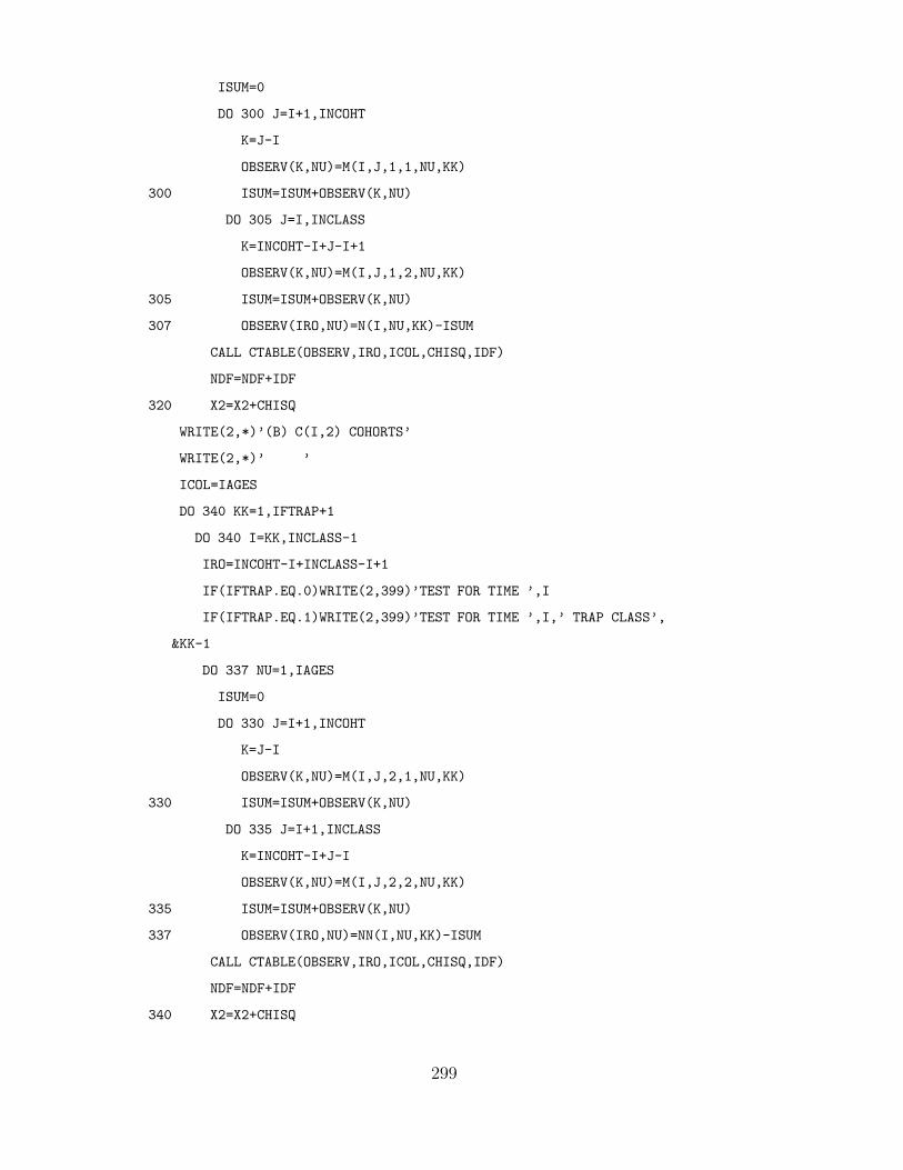
ISUM=0
DO 300 J=I+1,INCOHT
K=J-I
OBSERV(K,NU)=M(I,J,1,1,NU,KK)
300 ISUM=ISUM+OBSERV(K,NU)
DO 305 J=I,INCLASS
K=INCOHT-I+J-I+1
OBSERV(K,NU)=M(I,J,1,2,NU,KK)
305 ISUM=ISUM+OBSERV(K,NU)
307 OBSERV(IRO,NU)=N(I,NU,KK)-ISUM
CALL CTABLE(OBSERV,IRO,ICOL,CHISQ,IDF)
NDF=NDF+IDF
320 X2=X2+CHISQ
WRITE(2,*)’(B) C(I,2) COHORTS’
WRITE(2,*)’ ’
ICOL=IAGES
DO 340 KK=1,IFTRAP+1
DO 340 I=KK,INCLASS-1
IRO=INCOHT-I+INCLASS-I+1
IF(IFTRAP.EQ.0)WRITE(2,399)’TEST FOR TIME ’,I
IF(IFTRAP.EQ.1)WRITE(2,399)’TEST FOR TIME ’,I,’ TRAP CLASS’,
&KK-1
DO 337 NU=1,IAGES
ISUM=0
DO 330 J=I+1,INCOHT
K=J-I
OBSERV(K,NU)=M(I,J,2,1,NU,KK)
330 ISUM=ISUM+OBSERV(K,NU)
DO 335 J=I+1,INCLASS
K=INCOHT-I+J-I
OBSERV(K,NU)=M(I,J,2,2,NU,KK)
335 ISUM=ISUM+OBSERV(K,NU)
337 OBSERV(IRO,NU)=NN(I,NU,KK)-ISUM
CALL CTABLE(OBSERV,IRO,ICOL,CHISQ,IDF)
NDF=NDF+IDF
340 X2=X2+CHISQ
299

CALL CDTR(X2,NDF,SVALUE,IERR2)
PVALUE=1-SVALUE
WRITE(2,*)’OMNIBUS AGE-DEPENDENCE TEST’
WRITE(UNIT=2,FMT=’(A8,F8.4,3X,A5,I3,3X,A4,F6.4)’)
&’CHISQ = ’,X2,’DF = ’,NDF,’P =’,PVALUE
WRITE(UNIT=2,FMT=’(A5)’)’ ’
390 CONTINUE
C
C CARRY OUT OMNIBUS TRAP-DEPENDENCE TEST
C
IF(IFTRAP.EQ.0) GOTO 450
X2=0.
NDF=0
499 FORMAT(A14,1X,I2,A4,1X,I2)
WRITE(2,*)’ ’
WRITE(2,*)’OMNIBUS TRAP-DEPENDENCE TEST’
WRITE(2,*)’---------------------------’
WRITE(2,*)’(A) C(I,1) COHORTS’
WRITE(2,*)’ ’
ICOL=2
DO 420 NU=1,IAGES
DO 420 I=2,INCOHT
IRO=INCOHT-I+INCLASS-I+2
IF(IAGES.EQ.1)WRITE(2,499)’TEST FOR TIME ’,I
IF(IAGES.GT.1)WRITE(2,499)’TEST FOR TIME ’,I,’ AGE’,NU-1
DO 407 KK=1,2
ISUM=0
DO 400 J=I+1,INCOHT
K=J-I
OBSERV(K,KK)=M(I,J,1,1,NU,KK)
400 ISUM=ISUM+OBSERV(K,KK)
DO 405 J=I,INCLASS
K=INCOHT-I+J-I+1
OBSERV(K,KK)=M(I,J,1,2,NU,KK)
300

405 ISUM=ISUM+OBSERV(K,KK)
407 OBSERV(IRO,KK)=N(I,NU,KK)-ISUM
CALL CTABLE(OBSERV,IRO,ICOL,CHISQ,IDF)
NDF=NDF+IDF
420 X2=X2+CHISQ
WRITE(2,*)’(B) C(I,2) COHORTS’
WRITE(2,*)’ ’
ICOL=2
DO 440 NU=1,IAGES
DO 440 I=2,INCLASS-1
IRO=INCOHT-I+INCLASS-I+1
IF(IAGES.EQ.1)WRITE(2,499)’TEST FOR TIME ’,I
IF(IAGES.GT.1)WRITE(2,499)’TEST FOR TIME ’,I,’AGE ’,NU-1
DO 437 KK=1,2
ISUM=0
DO 430 J=I+1,INCOHT
K=J-I
OBSERV(K,KK)=M(I,J,2,1,NU,KK)
430 ISUM=ISUM+OBSERV(K,KK)
DO 435 J=I+1,INCLASS
K=INCOHT-I+J-I
OBSERV(K,KK)=M(I,J,2,2,NU,KK)
435 ISUM=ISUM+OBSERV(K,KK)
437 OBSERV(IRO,KK)=NN(I,NU,KK)-ISUM
CALL CTABLE(OBSERV,IRO,ICOL,CHISQ,IDF)
NDF=NDF+IDF
440 X2=X2+CHISQ
CALL CDTR(X2,NDF,SVALUE,IERR2)
PVALUE=1-SVALUE
WRITE(2,*)’OMNIBUS TRAP-DEPENDENCE TEST’
WRITE(UNIT=2,FMT=’(A8,F8.4,3X,A5,I3,3X,A4,F6.4)’)
&’CHISQ = ’,X2,’DF = ’,NDF,’P =’,PVALUE
WRITE(UNIT=2,FMT=’(A5)’)’ ’
301

450 CONTINUE
END
Subroutine SUMMARY
SUBROUTINE SUMMARY(INCOHT,INCLASS,IAGES,IFTRAP,M,RI1,RI2,CI,OI,
&R1,R2,NSUM,NNSUM,R1SUM,R2SUM,CSUM,OSUM,Z,ZSUM,T,R,TSUM,RSUM)
C
C THIS SUBROUTINE RETURNS THE SUMMARY STATISTICS
C
INCLUDE ’MPAR’
C INITIALISE TO ZERO
DO 100 NU=1,IAGES
DO 100 KK=1,IFTRAP+1
DO 100 I=1,INCLASS
RI1(I,NU,KK)=0
RI2(I,NU,KK)=0
CI(I+1,NU+1,KK)=0
100 OI(I,NU,KK)=0
C
C FIND ROW TOTALS RI1(I,NU,OMEGA) AND RI2(I,NU,OMEGA)
C
DO 700 NU=1,IAGES
DO 500 OMEGA=1,IFTRAP+1
DO 500 I=1,MAX(INCOHT,INCLASS-1)
DO 450 J=2,INCOHT
450 RI1(I,NU,OMEGA)=RI1(I,NU,OMEGA)+M(I,J,1,1,NU,OMEGA)
DO 460 J=1,INCLASS
460 RI1(I,NU,OMEGA)=RI1(I,NU,OMEGA)+M(I,J,1,2,NU,OMEGA)
DO 470 J=2,INCOHT
470 RI2(I,NU,OMEGA)=RI2(I,NU,OMEGA)+M(I,J,2,1,NU,OMEGA)
DO 480 J=2,INCLASS
480 RI2(I,NU,OMEGA)=RI2(I,NU,OMEGA)+M(I,J,2,2,NU,OMEGA)
500 CONTINUE
302

C
C FIND COLUMN TOTALS - NOTE THESE ARE PARTIAL
C
DO 550 J=2,INCOHT
DO 550 I=1,J-1
ICLASS=NU+J-I
IF(ICLASS.GT.IAGES+1)ICLASS=IAGES+1
IF(IFTRAP.EQ.1) THEN
IF(I.EQ.J-1)THEN
CI(J,ICLASS,1)=M(I,J,1,1,NU,1)+M(I,J,2,1,NU,1)
CI(J,ICLASS,2)=CI(J,ICLASS,2)+M(I,J,1,1,NU,2)
& +M(I,J,2,1,NU,2)
ELSE
CI(J,ICLASS,2)=CI(J,ICLASS,2)+M(I,J,1,1,NU,2)
& +M(I,J,2,1,NU,2)+M(I,J,1,1,NU,1)+M(I,J,2,1,NU,1)
ENDIF
GOTO 550
ENDIF
CI(J,ICLASS,1)=CI(J,ICLASS,1)+M(I,J,1,1,NU,1)
& +M(I,J,2,1,NU,1)
550 CONTINUE
DO 560 J=1,INCLASS
DO 560 I=1,J
ICLASS=NU+J-I
IF(ICLASS.GT.IAGES)ICLASS=IAGES
IF(IFTRAP.EQ.1)THEN
IF(I.EQ.J) THEN
OI(J,ICLASS,1)=M(I,J,1,2,NU,1)+M(I,J,2,2,NU,1)
OI(J,ICLASS,2)=OI(J,ICLASS,2)+M(I,J,1,2,NU,2)
& +M(I,J,2,2,NU,2)
ELSE
OI(J,ICLASS,2)=OI(J,ICLASS,2)+M(I,J,1,2,NU,2)
& +M(I,J,2,2,NU,2)+M(I,J,1,2,NU,1)+M(I,J,2,2,NU,1)
ENDIF
303

GOTO 560
ENDIF
OI(J,ICLASS,1)=OI(J,ICLASS,1)+M(I,J,1,2,NU,1)+
& M(I,J,2,2,NU,1)
560 CONTINUE
700 CONTINUE
C
C COMPUTE MARGINAL TOTALS
C
DO 740 OMEGA=1,2
DO 710 I=1,INCOHT
DO 710 NU=1,IAGES
R1(I,OMEGA)=R1(I,OMEGA)+RI1(I,NU,OMEGA)
710 NSUM(I,OMEGA)=NSUM(I,OMEGA)+N(I,NU,OMEGA)
DO 720 I=1,INCLASS-1
DO 720 NU=1,IAGES
NNSUM(I,OMEGA)=NNSUM(I,OMEGA)+NN(I,NU,OMEGA)
720 R2(I,OMEGA)=R2(I,OMEGA)+RI2(I,NU,OMEGA)
DO 730 I=2,INCOHT
DO 730 NU=1,IAGES+1
730 CSUM(I,OMEGA)=CSUM(I,OMEGA)+CI(I,NU,OMEGA)
DO 740 I=1,INCLASS
DO 740 NU=1,IAGES
740 OSUM(I,OMEGA)=OSUM(I,OMEGA)+OI(I,NU,OMEGA)
C
C NOW COMPUTE Z(I)’S
C
Z(1,1,1)=0
Z(1,1,2)=0
IF(IFTRAP.EQ.1)THEN
DO 750 NU=2,IAGES
Z(1,NU,2)=0
DO 750 I=2,INCLASS
Z(I,NU,1)=RI1(I-1,NU-1,1)+RI2(I-1,NU-1,1)-CI(I,NU,1)
304

& -OI(I-1,NU-1,1)
C PRINT*,RI1(I-1,NU-1,1),RI2(I-1,NU-1,1),CI(I,NU,1),
C & -OI(I-1,NU-1,1)
750 Z(I,NU,2)=Z(I-1,NU-1,1)+Z(I-1,NU-1,2)+RI1(I-1,NU-1,2)
& +RI2(I-1,NU-1,2)-CI(I,NU,2)-OI(I-1,NU-1,2)
DO 760 I=2,INCLASS
Z(I,IAGES+1,1)=RI1(I-1,IAGES,1)+RI2(I-1,IAGES,1)
& -CI(I,IAGES+1,1)-OI(I-1,IAGES,1)
760 Z(I,IAGES+1,2)=Z(I-1,IAGES,1)+Z(I-1,IAGES+1,1)+
& Z(I-1,IAGES,2)+Z(I-1,IAGES+1,2)+RI1(I-1,IAGES,2)+
& RI2(I-1,IAGES,2)-CI(I,IAGES+1,2)-OI(I-1,IAGES,2)
ELSE
DO 761 NU=2,IAGES
Z(1,NU,1)=0
DO 761 I=2,INCLASS
761 Z(I,NU,1)=Z(I-1,NU-1,1)+RI1(I-1,NU-1,1)
& +RI2(I-1,NU-1,1)-CI(I,NU,1)-OI(I-1,NU-1,1)
DO 762 I=2,INCLASS
762 Z(I,IAGES+1,1)=Z(I-1,IAGES,1)+Z(I-1,IAGES+1,1)
& +RI1(I-1,IAGES,1)+
& RI2(I-1,IAGES,1)-CI(I,IAGES+1,1)-OI(I-1,IAGES,1)
ENDIF
C
C COMPUTE R(I)’S
C
IF(IFTRAP.EQ.1)THEN
DO 764 I=1,INCLASS
R(I,1,1)=RI1(I,1,1)
R(I,1,2)=RI1(I,1,2)
R(I,IAGES,1)=RI1(I,IAGES,1)
R(I,IAGES,2)=Z(I,IAGES,1)+Z(I,IAGES+1,1)+Z(I,IAGES,2)+
& Z(I,IAGES+1,2)+RI1(I,IAGES,2)
305

764 IF(I.GT.INCOHT+1)R(I,IAGES,2)=Z(I,IAGES,1)+Z(I,IAGES+1,1)+
& Z(I,IAGES,2)+Z(I,IAGES+1,2)
DO 765 NU=2,IAGES-1
DO 765 I=1,INCLASS
R(I,NU,1)=RI1(I,NU,1)
R(I,NU,2)=Z(I,NU,1)+Z(I,NU,2)+RI1(I,NU,2)
765 IF(I.GT.INCOHT+1)R(I,NU,2)=Z(I,NU,1)+Z(I,NU,2)
ELSE
DO 766 I=1,INCLASS
R(I,1,1)=RI1(I,1,1)
R(I,IAGES,1)=Z(I,IAGES,1)+Z(I,IAGES+1,1)+RI1(I,IAGES,1)
766 IF(I.GT.INCOHT+1)R(I,IAGES,1)=Z(I,IAGES,1)+Z(I,IAGES+1,1)
DO 767 NU=2,IAGES-1
DO 767 I=1,INCLASS
R(I,NU,1)=Z(I,NU,1)+RI1(I,NU,1)
767 IF(I.GT.INCOHT+1)R(I,NU,1)=Z(I,NU,1)
ENDIF
C
C COMPUTE T(I)’S
C
DO 768 OMEGA=1,IFTRAP+1
DO 768 NU=2,IAGES+1
DO 768 I=1,INCLASS
768 T(I,NU,OMEGA)=Z(I,NU,OMEGA)+CI(I,NU,OMEGA)
C
C COMPUTE MARGINALS FOR Z(I)’S, T(I)’S AND R(I)’S
C
DO 772 OMEGA=1,IFTRAP+1
DO 770 I=2,INCLASS
DO 770 NU=1,IAGES+1
770 ZSUM(I,OMEGA)=ZSUM(I,OMEGA)+Z(I,NU,OMEGA)
DO 771 I=1,INCLASS
DO 771 NU=1,IAGES
771 RSUM(I,OMEGA)=RSUM(I,OMEGA)+R(I,NU,OMEGA)
306

DO 772 I=2,INCOHT
DO 772 NU=1,IAGES+1
772 TSUM(I,OMEGA)=TSUM(I,OMEGA)+T(I,NU,OMEGA)
RETURN
END
Subroutime GOF
SUBROUTINE GOF(M,RI1,RI2,CI,OI,T,R,IAGES,INCOHT,INCLASS,IFTRAP,
&X2,NDF,CPOOL)
IMPLICIT DOUBLE PRECISION (A-H,O-Z)
C
C GOF COMPUTES GOODNESS OF FIT TESTS STATISTIC
C
C IFTRAP = 0 MODEL WITH NO TRAP RESPONSE
C 1 MODEL WITH TRAP RESPONSE
C
INCLUDE ’MPAR’
C
C LOCAL VARIABLES
C
1 FORMAT(20I4)
INTEGER CPOOL
IK=IFTRAP+1
C
C OBTAIN PARTIAL COLUMN TOTALS
C
CALL MPARTIAL(M,MP,INCOHT,INCLASS,IAGES,IFTRAP)
C
C COMPONENT 1 T(I+1) // C(I+1)
C
WRITE(UNIT=2,FMT=’(A5)’)’ ’
WRITE(UNIT=2,FMT=’(A23)’)’OVERALL GOODNESS-OF-FIT’
WRITE(UNIT=2,FMT=’(A20)’)’(A) T(I+1) // C(I+1)’
307

X2=0.
NDF=0
IRO=2
ICOL=2
IF(IFTRAP.EQ.1) THEN
DO 10 NU=1,IAGES
DO 10 K=1,2
C
C NB IF FIRST AGE CLASS AND SECOND TRAP CLASS, TABLE DOES NOT EXIST
C
C IF(NU.EQ.1 .AND. K.EQ.2)GOTO 10
DO 10 I=K,INCOHT-2
IF(IAGES.GT.1 .AND. IFTRAP.EQ.1) THEN
WRITE(UNIT=2,FMT=’(A3,I3,1X,A10,I2,1X,A4,I3)’)
& ’AGE’,NU,’TRAP CLASS’,K-1,’YEAR’,I
ELSEIF(IAGES.GT.1 .AND. IFTRAP.EQ.0)THEN
WRITE(UNIT=2,FMT=’(A3,I3,1X,A4,I3)’)
& ’AGE’,NU,’YEAR’,I
ELSEIF(IAGES.EQ.1 .AND. IFTRAP.EQ.1)THEN
WRITE(UNIT=2,FMT=’(A10,I2,1X,A4,I3)’)
& ’TRAP CLASS’,K-1,’YEAR’,I
ELSE
WRITE(UNIT=2,FMT=’(A4,I3)’)’YEAR’,I
ENDIF
OBSERV(1,1)=MP(I,I+1,1,NU,K)
OBSERV(1,2)=M(I,I+1,2,1,NU,K)
OBSERV(2,1)=R(I,NU,K)-OI(I,NU,K)-OBSERV(1,1)
OBSERV(2,2)=RI2(I,NU,K)-OBSERV(1,2)
CALL CTABLE(OBSERV,IRO,ICOL,CHISQ,IDF)
X2=X2+CHISQ
NDF=NDF+IDF
IRO=2
ICOL=2
10 CONTINUE
ELSE
308

DO 20 NU=1,IAGES
DO 20 I=1,INCOHT-1
IF(IAGES.EQ.1) THEN
WRITE(UNIT=2,FMT=’(A4,I3)’)’YEAR’,I
ELSE
WRITE(UNIT=2,FMT=’(A3,I3,1X,A4,I3)’)
& ’AGE’,NU,’YEAR’,I
ENDIF
OBSERV(1,1)=M(I,I+1,2,1,NU,1)+M(I,I+1,2,1,NU,2)
OBSERV(1,2)=CI(I+1,NU+1,1)-M(I,I+1,2,1,NU,1)+
& CI(I+1,NU+1,2)-M(I,I+1,2,1,NU,2)
OBSERV(2,1)=RI2(I,NU,1)+RI2(I,NU,2)-OBSERV(1,1)
OBSERV(2,2)=R(I,NU,1)-OI(I,NU,1)+R(I,NU,2)-OI(I,NU,2)
& -OBSERV(1,2)
CALL CTABLE(OBSERV,IRO,ICOL,CHISQ,IDF)
X2=X2+CHISQ
NDF=NDF+IDF
IRO=2
20 ICOL=2
ENDIF
C
C NOW COMPUTE R(I) // [M(I,J,K,L,NU,OMEGA)] COMPONENTS
C
WRITE(UNIT=2,FMT=’(A32)’)’(B) R(I+1) // MP(I,J,K,NU,OMEGA)’
IRO=(INCOHT-1)+INCLASS
ICOL=3
DO 360 NU=1,IAGES-1
IF(IAGES.GT.1) THEN
WRITE(UNIT=2,FMT=’(A3,I3,1X,A4,I3)’)
& ’AGE’,NU,’YEAR’,1
ELSE
WRITE(UNIT=2,FMT=’(A4,I3)’)’YEAR’,1
ENDIF
DO 300 J=3,INCOHT
309

K=J-2
OBSERV(K,1)=MP(1,J,1,NU,1)
OBSERV(K,2)=M(1,J,2,1,NU,1)
OBSERV(K,3)=M(2,J,1,1,NU+1,1)
300 IF(IFTRAP.EQ.1)OBSERV(K,3)=M(2,J,1,1,NU+1,2)
DO 310 J=2,INCLASS
K=INCOHT-2+J-1
OBSERV(K,1)=MP(1,J,2,NU,1)
OBSERV(K,2)=M(1,J,2,2,NU,1)
OBSERV(K,3)=M(2,J,1,2,NU+1,1)
310 IF(IFTRAP.EQ.1)OBSERV(K,3)=M(2,J,1,2,NU+1,2)
C
C IF CAPTURE/OBSERVATIONS FROM ANIMALS LAST RELEASED FOLLOWING OBSERVATION
C ARE SPARSE, CPOOL CAN BE SET TO 1 TO POOL DATA FROM THESE ANIMALS
C WITH DATA FROM ANIMALS LAST RELEASED FOLLOWING CAPTURE
C
IF(CPOOL.EQ.1) THEN
DO 315 II=1,IRO
OBSERV(II,1)=OBSERV(II,1)+OBSERV(II,2)
315 OBSERV(II,2)=OBSERV(II,3)
ICOL=2
ENDIF
CALL CTABLE(OBSERV,IRO,ICOL,CHISQ,IDF)
X2=X2+CHISQ
NDF=NDF+IDF
C
C NOW DO FOR THE REMAINING YEARS
C
IRO=(INCOHT-I-1)+INCLASS-J-1
ICOL=2*(IFTRAP+1)+1
IMAX=INCOHT-2
IF(INCLASS.GT.INCOHT)IMAX=INCOHT-1
DO 360 I=2,INCOHT-2
IF(IAGES.GT.1)THEN
WRITE(UNIT=2,FMT=’(A3,I3,1X,A4,I3)’)
310

& ’AGE’,NU,’YEAR’,I
ELSE
WRITE(UNIT=2,FMT=’(A4,I3)’)’YEAR’,I
ENDIF
DO 330 J=I+2,INCOHT
K=J-I-1
INDEX=1
DO 320 KK=1,IFTRAP+1
C
C SKIP IF FIRST AGE CLASS AND SECOND TRAP CLASS
C
IF(NU.EQ.1 .AND. KK.EQ.2) GOTO320
OBSERV(K,INDEX)=MP(I,J,1,NU,KK)
INDEX=INDEX+1
OBSERV(K,INDEX)=M(I,J,2,1,NU,KK)
INDEX=INDEX+1
320 CONTINUE
330 OBSERV(K,INDEX)=M(I+1,J,1,1,NU+1,1)
DO 350 J=I+1,INCOHT
K=INCOHT-I-1+J-1
INDEX=1
DO 340 KK=1,IFTRAP+1
IF(NU.EQ.1 .AND. KK.EQ.2) GOTO340
OBSERV(K,INDEX)=MP(I,J,2,NU,KK)
INDEX=INDEX+1
OBSERV(K,INDEX)=M(I,J,2,2,NU,KK)
INDEX=INDEX+1
340 CONTINUE
350 OBSERV(K,2*(INDEX)+1)=M(I+1,J,1,2,NU+1,IK)
C
C NOW POOL COLUMNS IF REQUIRED
C
IF(CPOOL.EQ.1) THEN
IF(ITRAP.EQ.0) THEN
DO 355 II=1,IRO
OBSERV(II,1)=OBSERV(II,1)+OBSERV(II,2)
311

355 OBSERV(II,2)=OBSERV(II,3)
ICOL=2
ELSE
DO 356 II=1,IRO
OBSERV(II,1)=OBSERV(II,1)+OBSERV(II,2)
OBSERV(II,2)=OBSERV(II,3)+OBSERV(II,4)
356 OBSERV(II,3)=OBSERV(II,5)
ICOL=2
ENDIF
ENDIF
CALL CTABLE(OBSERV,IRO,ICOL,CHISQ,IDF)
X2=X2+CHISQ
NDF=NDF+IDF
IRO=(INCOHT-2)+INCLASS-1
360 ICOL=2*(IFTRAP+1)+1
C
C NOW FOR THE LAST AGE GROUP
C
WRITE(UNIT=2,FMT=’(A3,I3,1X,A4,I3)’)
& ’AGE’,IAGES,’YEAR’,1
ICOL=5
IRO=INCOHT-2+INCLASS-1
DO 370 J=3,INCOHT
K=J-2
IF(IAGES.EQ.1) THEN
ICOL=3
OBSERV(K,1)=MP(1,J,1,IAGES,1)
OBSERV(K,2)=M(1,J,2,1,IAGES,1)
OBSERV(K,3)=M(2,J,1,1,IAGES,1)
IF(IFTRAP.EQ.1)OBSERV(K,3)=M(2,J,1,1,IAGES,2)
ELSE
OBSERV(K,1)=MP(1,J,1,IAGES-1,1)
OBSERV(K,2)=MP(1,J,1,IAGES,1)
OBSERV(K,3)=M(1,J,2,1,IAGES-1,1)
OBSERV(K,4)=M(1,J,2,1,IAGES,1)
312

OBSERV(K,5)=M(2,J,1,1,IAGES,1)
IF(IFTRAP.EQ.1)OBSERV(K,5)=M(2,J,1,1,IAGES,2)
370 ENDIF
DO 380 J=2,INCLASS
K=INCOHT-2+J-1
IF(IAGES.EQ.1)THEN
OBSERV(K,1)=MP(1,J,2,IAGES,1)
OBSERV(K,2)=M(1,J,2,2,IAGES,1)
OBSERV(K,3)=M(2,J,1,2,IAGES,1)
IF(IFTRAP.EQ.1)OBSERV(K,3)=M(2,J,1,2,IAGES,2)
ELSE
OBSERV(K,1)=MP(1,J,2,IAGES-1,1)
OBSERV(K,2)=MP(1,J,2,IAGES,1)
OBSERV(K,3)=M(1,J,2,2,IAGES-1,1)
OBSERV(K,4)=M(1,J,2,2,IAGES,1)
OBSERV(K,5)=M(2,J,1,2,IAGES,1)
IF(IFTRAP.EQ.1)OBSERV(K,5)=M(2,J,1,2,IAGES,2)
380 ENDIF
C
C NOW POOL COLUMNS IF REQUIRED
C
IF(CPOOL.EQ.1) THEN
DO 385 II=1,IRO
IF(IAGES.EQ.1)THEN
OBSERV(II,1)=OBSERV(II,1)+OBSERV(II,2)
OBSERV(II,2)=OBSERV(II,3)
ICOL=2
ELSE
OBSERV(II,1)=OBSERV(II,1)+OBSERV(II,3)
OBSERV(II,2)=OBSERV(II,2)+OBSERV(II,4)
OBSERV(II,3)=OBSERV(II,5)
ICOL=3
385 ENDIF
ENDIF
CALL CTABLE(OBSERV,IRO,ICOL,CHISQ,IDF)
X2=X2+CHISQ
313

NDF=NDF+IDF
C
C NOW DO FOR THE REMAINING YEARS
C
IMAX=INCOHT-2
IF(INCLASS.GT.INCOHT)IMAX=INCOHT-1
DO 430 I=2,IMAX
IRO=(INCOHT-I-1)+INCLASS-I
WRITE(UNIT=2,FMT=’(A3,I3,1X,A4,I3)’)
& ’AGE’,IAGES,’YEAR’,I
DO 400 J=I+2,INCOHT
K=J-I-1
INDEX=1
DO 390 KK=1,IFTRAP+1
ISTART=IAGES-1
IF(IAGES.EQ.1)ISTART=1
DO 390 NU=ISTART,IAGES
IF(NU.EQ.1 .AND.KK.EQ.2) GOTO 390
OBSERV(K,INDEX)=MP(I,J,1,NU,KK)
INDEX=INDEX+1
OBSERV(K,INDEX)=M(I,J,2,1,NU,KK)
INDEX=INDEX+1
390 CONTINUE
400 OBSERV(K,INDEX)=M(I+1,J,1,1,IAGES,IK)
DO 420 J=I+1,INCLASS
K=INCOHT-I-1+J-I
INDEX=1
DO 410 KK=1,IFTRAP+1
DO 410 NU=ISTART,IAGES
IF(NU.EQ.1 .AND.KK.EQ.2) GOTO 410
OBSERV(K,INDEX)=MP(I,J,2,NU,KK)
INDEX=INDEX+1
OBSERV(K,INDEX)=M(I,J,2,2,NU,KK)
INDEX=INDEX+1
314

410 CONTINUE
420 OBSERV(K,INDEX)=M(I+1,J,1,2,IAGES,IK)
C
C NOW POOL COLUMNS IF REQUIRED
C
IF(CPOOL.EQ.1)THEN
DO 428 II=1,IRO
INDEX=1
INDX=1
DO 425 KK=1,IFTRAP+1
ISTART=IAGES-1
IF(IAGES.EQ.1)ISTART=1
DO 425 NU=ISTART,IAGES
OBSERV(II,INDEX)=OBSERV(II,INDX)+OBSERV(II,INDX+1)
INDEX=INDEX+1
425 INDX=INDX+2
428 OBSERV(II,INDEX)=OBSERV(II,INDX)
ENDIF
ICOL=INDEX
CALL CTABLE(OBSERV,IRO,ICOL,CHISQ,IDF)
X2=X2+CHISQ
NDF=NDF+IDF
430 IRO=(INCOHT-I-1)+INCLASS-I
C
C IF THERE ARE OBSERVATIONS BEYOND THE LAST CAPTURE PERIOD COMPUTE
C ADDITIONAL TERM
C
IF(INCLASS.LE.INCOHT+1)GOTO 600
IRO=INCLASS-INCOHT
I=INCOHT
DO 550 NU=1,IAGES
IF(IAGES.NE.1 .AND. NU.EQ.1.AND.K.EQ.2)GOTO 550
DO 540 J=I+1,INCLASS
315

K=J-I
INDEX=1
DO 540 KK=1,IFTRAP+1
IF(NU.EQ.1.AND.KK.EQ.2)GOTO 540
OBSERV(K,INDEX)=MP(I,J,2,NU,KK)
INDEX=INDEX+1
OBSERV(K,INDEX)=M(I,J,2,2,NU,KK)
INDEX=INDEX+1
540 CONTINUE
ICOL=INDEX
550 CONTINUE
C
C NOW POOL COLUMNS IF REQUIRED
C
IF(CPOOL.EQ.1)THEN
DO 560 II=1,IRO
INDEX=1
INDX=1
DO 555 KK=1,IFTRAP+1
ISTART=IAGES-1
IF(IAGES.EQ.1)ISTART=1
DO 555 NU=ISTART,IAGES
OBSERV(II,INDEX)=OBSERV(II,INDX)+OBSERV(II,INDX+1)
INDEX=INDEX+1
555 INDX=INDX+2
560 OBSERV(II,INDEX)=OBSERV(II,INDX)
ENDIF
ICOL=INDEX
CALL CTABLE(OBSERV,IRO,ICOL,CHISQ,IDF)
X2=X2+CHISQ
NDF=NDF+IDF
IRO=(INCOHT-I-1)+INCLASS-I
600 CONTINUE
WRITE(UNIT=2,FMT=’(A42)’)’TEST STATISTIC FOR OVERALL GOODNESS-OF-F
316

&IT’
IF(NDF.EQ.0)WRITE(UNIT=2,FMT=’(A47)’)’ZERO DEGREES OF FREEDOM AFTE
&R POOLING’
CALL CDTR(X2,NDF,SVALUE,IERR2)
PVALUE=1-SVALUE
WRITE(UNIT=2,FMT=’(A8,F8.4,3X,A5,I3,3X,A4,F6.4)’)
&’CHISQ = ’,X2,’DF = ’,NDF,’P =’,PVALUE
RETURN
END
Subroutine CTABLE
C COMPUTES CONTINGENCY TABLE TEST STATISTIC
SUBROUTINE CHI(OBSERV,EXPECT,IROWS,ICOLS,CHISQ,IERR)
INCLUDE ’MPAR’
IMPLICIT DOUBLE PRECISION (A-H,O-Z)
INTEGER ISKIP(MXCLAS*2),OBSERV2(MXCLAS*2,MXCOL),MM1(MXCLAS*2),
&MM2(MXCOL)
DOUBLE PRECISION CHISQ
INTEGER NDF
C
C OBSERV - ARRAY OF OBSERVED CELL FREQUENCIES
C EXPECT - ARRAY OF EXPECTED CELL FREQUENCIES
C IRO - THE NUMBER OF ROWS IN THE TABLE
C ICOL - THE NUMBER OF COLUMNS IN THE TABLE
C NDF - NUMBER OF DEGREES OF FREEDOM IN TABLE
C CHISQ - CALCULATED CHI-SQUARE STATISTIC AFTER POOLING
C IERR - AN ERROR INDICATOR VARIABLE
C - IERR = 0 ... NO ERROR
C - IERR = 1 ... TOO FEW ROWS REMAINING AFTER POOLING
C TO COMPUTE CHI-SQUARE STATISTIC
C
IERR=0
C
317

C FIRST ELIMINATE ROWS OR COLUMNS WITH ZERO MARGINALS
C
DO 5 I=1,IROWS
DO 5 J=1,ICOLS
MM1(I)=MM1(I)+OBSERV(I,J)
5 MM2(J)=MM2(J)+OBSERV(I,J)
INDEX=1
DO 10 I=1,IROWS
IF(MM1(I).NE.0)THEN
DO 7 J=1,IROWS
7 OBSERV(INDEX,J)=OBSERV(I,J)
INDEX=INDEX+1
10 ENDIF
IROWS=INDEX-1
INDEX=1
DO 15 J=1,ICOLS
IF(MM2(J).NE.0)THEN
DO 12 I=1,IRO
12 OBSERV(I,INDEX)=OBSERV(I,J)
INDEX=INDEX+1
15 ENDIF
ICOLS=INDEX-1
C
C CALL EXPECT TO FIND EXPECTED VALUES
C
CALL EVALUES(OBSERV,EXPECT,IROWS,ICOLS)
C
C POOL ROWS BASED ON EXPECTED VALUES
C
318

C
C CYCLE UNTIL NO MORE ROWS ARE POOLED (IFLAG REMAINS AT 0)
C
DMIN=2.
30 CONTINUE
IFLAG=0
C
C ASSIGN OBSERV TO OBSERV2
C
DO 31 I=1,IROWS
DO 31 J=1,ICOLS
31 OBSERV2(I,J)=OBSERV(I,J)
C
C ISKIP MUST BE RESET TO ZERO ON EACH PASS
C
DO 35 I=1,IROWS
35 ISKIP(I)=0
DO 60 I=1,IROWS
DO 50 J=1,ICOLS
IF(EXPECT(I,J).LT.DMIN) THEN
IFLAG=1
ISKIP(I)=1
IF(I.EQ.1) THEN
DO 40 K=1,ICOLS
40 OBSERV2(I+1,K)=OBSERV(I,K)+OBSERV(I+1,K)
ELSE
DO 45 K=1,ICOLS
45 OBSERV2(I-1,K)=OBSERV(I,K)+OBSERV(I-1,K)
ENDIF
GOTO 62
ENDIF
50 CONTINUE
60 CONTINUE
319

C
C IF POOLING HAS OCCURRED ASSIGN THE RELEVANT ROWS OF OBSERV2
C TO OBSERV
C
62 IF(IFLAG.EQ.0) GOTO 80
IT=0
DO 70 I=1,IROWS
IF(ISKIP(I).EQ.0)THEN
DO 65 J=1,ICOLS
65 OBSERV(I-IT,J)=OBSERV2(I,J)
ELSE
IT=IT+1
70 ENDIF
IROWS=IROWS-IT
C
C COMPUTE NEW EXPECTED VALUES AND REPEAT THE CYCLE
C
CALL EVALUES(OBSERV,EXPECT,IROWS,ICOLS)
GOTO 30
C
C NOW COMPUTE CHI-SQUARE STATISTIC
C
80 CHISQ=0.
IF(IROWS .LE. 1) THEN
IERR=1
GOTO 110
ENDIF
DO 100 I=1,IROWS
DO 100 J=1,ICOLS
100 CHISQ=CHISQ+((OBSERV(I,J)-EXPECT(I,J))**2)/EXPECT(I,J)
320

110 RETURN
END
Subroutine EVALUES
C COMPUTES CONTINGENCY TABLE EXPECTED VALUES
SUBROUTINE EVALUES(OBSERV,EXPECT,IRO,ICOL)
INCLUDE ’MPAR’
IMPLICIT DOUBLE PRECISION (A-H,O-Z)
INTEGER MARG1(MXCLAS+1),MARG2(MXCOL)
C
C FIND MARGINALS AND GRAND TOTAL
C
ITOTAL=0
C
C INITIALISE MARGINALS TO ZER
C
DO 5 I=1,IRO
5 MARG1(I)=0
DO 6 J=1,ICOL
6 MARG2(J)=0
DO 10 I=1,IRO
DO 10 J=1,ICOL
MARG1(I)=MARG1(I)+OBSERV(I,J)
MARG2(J)=MARG2(J)+OBSERV(I,J)
10 ITOTAL=ITOTAL+OBSERV(I,J)
C
C COMPUTE EXPECTED VALUES
C
C
C IF THERE ARE NO OBSERVATIONS SET EXPECTED VALUES TO ZERO TO AVOID
C DIVISION ERROR
321

C
IF(ITOTAL.EQ.0)THEN
DO 15 I=1,IRO
DO 15 J=1,ICOL
15 EXPECT(I,J)=0
GOTO 30
ENDIF
DO 20 I=1,IRO
DO 20 J=1,ICOL
20 EXPECT(I,J)=FLOAT(MARG1(I))*FLOAT(MARG2(J))/FLOAT(ITOTAL)
30 RETURN
END
subsubsectionSubroutine CDFCHI
C *DECK CDTR
C
C ..................................................................
C
C SUBROUTINE CDTR
C
C PURPOSE
C COMPUTES P(CHISQ) = PROBABILITY THAT THE RANDOM VARIABLE U,
C DISTRIBUTED ACCORDING TO THE CHI-SQUARE DISTRIBUTION WITH G
C DEGREES OF FREEDOM, IS LESS THAN OR EQUAL TO CHISQ. F(G,CHI
C ORDINATE OF THE CHI-SQUARE DENSITY AT CHISQ, IS ALSO COMPUTE
C
C USAGE
C CALL CDTR(CHISQ,IDF,SIGCHI,IER)
C
C DESCRIPTION OF PARAMETERS
C CHISQ - INPUT SCALAR FOR WHICH P(CHISQ) IS COMPUTED.
C IDF - NUMBER OF DEGREES OF FREEDOM OF THE CHI-SQUARE
C DISTRIBUTION. IDF IS AN INTEGER.
C SIGCHI - OUTPUT PROBABILITY.
C IER - RESULTANT ERROR CODE WHERE
322

C IER= 0 --- NO ERROR
C IER=-1 --- AN INPUT PARAMETER IS INVALID. X IS LESS
C THAN 0.0, OR IDF IS LESS THAN 0.0 OR GREATER
C THAN 2*10**(+5). P AND D ARE SET TO -1.E25.
C IER=-2 --- IDF = 0, P SET TO 0.
C IER=+1 --- INVALID OUTPUT. P IS LESS THAN ZERO OR
C GREATER THAN ONE, OR SERIES FOR T1 (SEE
C MATHEMATICAL DESCRIPTION) HAS FAILED TO
C CONVERGE. P IS SET TO 1.E25.
C
C SUBROUTINES AND FUNCTION SUBPROGRAMS REQUIRED
C NDTR
C
C METHOD
C
C THIS FUNCTION WAS LIFTED FROM "NWAY" WRITTEN BY THE STANFORD
C COMPUTATION CENTER. THE SCC BORROWED IT FROM JOHN MORRIS OF THE
C COMPUTER INSTITUTE FOR SOCIAL SCIENCE RESEARCH AT MICHIGAN STATE
C UNIVERSITY.
C
SUBROUTINE CDTR (CHISQ,IDF,SIGCHI,IER)
INTEGER IDF, IER
DOUBLE PRECISION CHISQ, SIGCHI
DOUBLE PRECISION FACT(0:30), ANSCHI, FF, P, XI, PP, TERM, ARGNRM,
1 GAM, TXX
INTEGER I
C
C FACTORIALS OF 0 THROUGH 30. .
DATA FACT /1.00000000000000D00,1.00000000000000D00,2.000000
1 00000000D00,6.00000000000000D00,2.40000000000000D01,1.20000000000
2 000D02,7.20000000000000D02,5.04000000000000D03,4.03200000000000D0
3 4,3.62880000000000D05,3.62880000000000D06,3.99168000000000D07,4.7
4 9001600000000D08,6.22702080000000D09,8.71782912000000D10,1.307674
5 36800000D12,2.09227898880000D13,3.55687428096000D14,6.40237370572
6 800D15,1.21645100408832D17,2.43290200817664D18,5.10909421717094D1
7 9,1.12400072777761D21,2.58520167388850D22,6.20448401733239D23,1.5
323

8 5112100433310D25,4.03291461126606D26,1.08888694504184D28,3.048883
9 44611714D29,8.84176199373970D30,2.65252859812191D32/
C
IER=0
ANSCHI=1.
IF (CHISQ.LT.0..OR.IDF.LT.0) THEN
IER=-1
SIGCHI=-1.D25
ELSE IF (IDF.EQ.0) THEN
IER=-2
SIGCHI=0.
ELSE IF (CHISQ+100..EQ.100.) THEN
IER=0
SIGCHI=0.
ELSE
C
C GT 60 D.F. OR CHI GT 100 - USE A NORMAL APPROXIMATION
IF (IDF.GT.60 .OR. CHISQ.GT.100.) THEN
ARGNRM=SQRT(2.D0*CHISQ)-SQRT(2.D0*DBLE(IDF)-1.D0)
CALL NDTR (ARGNRM,SIGCHI)
ELSE
FF=IDF-2
P=0.5*FF
XI=0.5*CHISQ
PP=P+2.0
TERM=XI/PP
DO 10 I=1,100
ANSCHI=ANSCHI+TERM
IF (ABS(TERM).LT.1.0D-6) GO TO 20
PP=PP+1.0
10 TERM=TERM*XI/PP
20 GAM=1.0
IF (MOD(IDF,2).EQ.0) THEN
GAM=FACT(IDF/2)
ELSE
30 DO 40 I=1,IDF,2
324

40 GAM=GAM*DBLE(I)*0.5D0
GAM=GAM*1.7724588509
ENDIF
TXX=(P+1.0)*LOG(XI)- XI + LOG(ANSCHI/GAM)
IF (TXX.LE.88.0) THEN
IF (TXX.GT.-88.0) THEN
ANSCHI=EXP(TXX)
ELSE
ANSCHI=0.
ENDIF
ELSE
ANSCHI=1.
ENDIF
C IF (ANSCHI.LT.0.) THEN
C ANSCHI=0.
C ELSEIF (ANSCHI.GT.1.) THEN
C ANSCHI=1.
C ENDIF
SIGCHI=ANSCHI
ENDIF
IF (SIGCHI.LT.0..OR.SIGCHI.GT.1.) THEN
IER=1
SIGCHI=1.D25
ENDIF
ENDIF
RETURN
END
C *DECK NDTR
C SUBROUTINE NDTR
C
C PURPOSE
C COMPUTES Y = P(X) = PROBABILITY THAT THE RANDOM VARIABLE U,
C DISTRIBUTED NORMALLY(0,1), IS LESS THAN OR EQUAL TO X.
C F(X), THE ORDINATE OF THE NORMAL DENSITY AT X, IS ALSO
C COMPUTED.
C
325

C USAGE
C CALL NDTR(X,P)
C
C DESCRIPTION OF PARAMETERS
C X--INPUT SCALAR FOR WHICH P(X) IS COMPUTED.
C P--OUTPUT PROBABILITY.
C
C REMARKS
C MAXIMUM ERROR IS 0.0000007.
C
C SUBROUTINES AND SUBPROGRAMS REQUIRED
C NONE
C
C METHOD
C BASED ON APPROXIMATIONS IN C. HASTINGS, APPROXIMATIONS FOR
C DIGITAL COMPUTERS, PRINCETON UNIV. PRESS, PRINCETON, N.J.,
C 1955. SEE EQUATION 26.2.17, HANDBOOK OF MATHEMATICAL
C FUNCTIONS, ABRAMOWITZ AND STEGUN, DOVER PUBLICATIONS, INC.,
C NEW YORK.
C
C ******************************************************************
C
SUBROUTINE NDTR (X,P)
DOUBLE PRECISION X,P,T,D
C
T=1.D0/(1.D0+.2316419D0*ABS(X))
IF (-X*X*0.5D0.LT.-700.D0) THEN
D=0.3989423D0*EXP(-700.D0)
ELSE
D=0.3989423D0*EXP(-X*X*0.5D0)
ENDIF
P=1.0D0-D*T*((((1.330274D0*T-1.821256D0)*T+1.781478D0)*T
1 -0.3565638D0)*T+0.3193815D0)
IF (X .LT. 0.D0) THEN
P=1.D0-P
ENDIF
326

20 RETURN
END
Subroutine MPARTIAL
SUBROUTINE MPARTIAL(M,MP,INCOHT,INCLASS,IAGES,IFTRAP)
IMPLICIT DOUBLE PRECISION (A-H,O-Z)
C
C RETURNS PARTIAL COLUMN TOTALS
C
C ICLASS = 1 ONE-AGE MODEL
C L L-AGE MODEL
C IFTRAP = 0 MODEL WITH NO TRAP RESPONSE
C 1 MODEL WITH TRAP RESPONSE
C
INCLUDE ’MPAR’
C
C INITIALIZE TO ZERO
C
DO 100 K=1,IFTRAP+1
DO 100 NU=1,IAGES
DO 100 I=1,INCOHT
DO 90 J=I+1,INCOHT
90 MP(I,J,1,NU,K)=0
DO 100 J=I,INCOHT
100 MP(I,J,2,NU,K)=0
DO 106 I=1,INCOHT
DO 105 J=I+1,INCOHT
MP(I,J,1,1,1)=M(I,J,1,1,1,1)
105 MP(I,J,1,1,2)=0
DO 106 J=I,INCLASS
MP(I,J,2,1,1)=M(I,J,1,2,1,1)
106 MP(I,J,2,1,2)=0
DO 130 NU=2,IAGES-1
327

DO 110 J=2,INCOHT
MP(1,J,1,NU,1)=M(1,J,1,1,NU,1)
MP(1,J,1,NU,2)=M(1,J,1,1,NU,2)
IF(J.NE.2)MP(2,J,1,NU,1)=M(2,J,1,1,NU,1)
110 IF(J.NE.2)MP(2,J,1,NU,2)=M(2,J,1,1,NU,2)+
& M(1,J,1,1,NU-1,1)+M(1,J,2,1,NU-1,1)
DO 112 J=1,INCLASS
MP(1,J,2,NU,1)=M(1,J,1,2,NU,1)
MP(1,J,2,NU,2)=M(1,J,1,2,NU,2)
IF(J.NE.1)MP(2,J,2,NU,1)=M(2,J,1,2,NU,1)
112 IF(J.NE.1)MP(2,J,2,NU,2)=M(2,J,1,2,NU,2)+M(1,J,1,2,NU-1,1)
& +M(1,J,2,2,NU-1,1)
DO 130 I=2,INCOHT-1
DO 122 J=I+2,INCOHT
MP(I+1,J,1,NU,1)=M(I+1,J,1,1,NU,1)
122 MP(I+1,J,1,NU,2)=M(I+1,J,1,1,NU,2)+MP(I,J,1,NU-1,1)+
& MP(I,J,1,NU-1,2)+M(I,J,2,1,NU-1,1)+M(I,J,2,1,NU-1,2)
C 122 MP(I+1,J,1,NU,2)=M(I+1,J,1,1,NU,2)+M(I,J,1,1,NU-1,1)+
C & M(I,J,1,1,NU-1,2)+M(I,J,2,1,NU-1,1)+M(I,J,2,1,NU-1,2)
DO 124 J=I+1,INCLASS
MP(I+1,J,2,NU,1)=M(I+1,J,1,2,NU,1)
124 MP(I+1,J,2,NU,2)=M(I+1,J,1,2,NU,2)+MP(I,J,2,NU-1,1)+
& MP(I,J,2,NU-1,2)+M(I,J,2,2,NU-1,1)+M(I,J,2,2,NU-1,2)
C 124 MP(I+1,J,2,NU,2)=M(I+1,J,1,2,NU,2)+M(I,J,1,2,NU-1,1)+
C & M(I,J,1,2,NU-1,2)+M(I,J,2,2,NU-1,1)+M(I,J,2,2,NU-1,2)
130 CONTINUE
C
C THEN DO FOR LAST AGE GROUP
C
DO 140 J=2,INCOHT
MP(1,J,1,IAGES,1)=M(1,J,1,1,IAGES,1)
MP(1,J,1,IAGES,2)=M(1,J,1,1,IAGES,2)
IF(J.NE.2)MP(2,J,1,IAGES,1)=M(2,J,1,1,IAGES,1)
IF (IAGES.EQ.1)THEN
328

IF(J.NE.2)MP(2,J,1,IAGES,2)=M(2,J,1,1,IAGES,2)+
& M(1,J,1,1,IAGES,1)+M(1,J,2,1,IAGES,1)
ELSE
IF(J.NE.2)MP(2,J,1,IAGES,2)=M(2,J,1,1,IAGES,2)
& +M(1,J,1,1,IAGES-1,1)+
& M(1,J,1,1,IAGES,1)+M(1,J,2,1,IAGES-1,1)+M(1,J,2,1,IAGES,1)
140 ENDIF
DO 150 J=1,INCLASS
MP(1,J,2,IAGES,1)=M(1,J,1,2,IAGES,1)
MP(1,J,2,IAGES,2)=M(1,J,1,2,IAGES,2)
IF(J.NE.1)MP(2,J,2,IAGES,1)=M(2,J,1,2,IAGES,1)
IF(IAGES.EQ.1)THEN
IF(J.NE.1)MP(2,J,2,IAGES,2)=M(2,J,1,2,IAGES,2)+
& M(1,J,1,2,IAGES,1)+M(1,J,2,2,IAGES,1)
ELSE
IF(J.NE.1)MP(2,J,2,IAGES,2)=M(2,J,1,2,IAGES,2)+
& M(1,J,1,2,IAGES-1,1)+
& M(1,J,1,2,IAGES,1)+M(1,J,2,2,IAGES-1,1)+M(1,J,2,2,IAGES,1)
150 ENDIF
DO 170 I=2,INCOHT-1
DO 160 J=I+2,INCOHT
MP(I+1,J,1,IAGES,1)=M(I+1,J,1,1,IAGES,1)
IF(IAGES.EQ.1) THEN
MP(I+1,J,1,IAGES,2)=M(I+1,J,1,1,IAGES,2)+
& MP(I,J,1,IAGES,2)+MP(I,J,1,IAGES,1)+
& M(I,J,2,1,IAGES,2)+M(I,J,2,1,IAGES,1)
ELSE
MP(I+1,J,1,IAGES,2)=M(I+1,J,1,1,IAGES,2)+
& MP(I,J,1,IAGES-1,2)+MP(I,J,1,IAGES,2)
& +MP(I,J,1,IAGES-1,1)+MP(I,J,1,IAGES,1)
& +M(I,J,2,1,IAGES-1,2)+M(I,J,2,1,IAGES,2)
& +M(I,J,2,1,IAGES-1,1)+M(I,J,2,1,IAGES,1)
160 ENDIF
DO 170 J=I+1,INCLASS
MP(I+1,J,2,IAGES,1)=M(I+1,J,1,2,IAGES,1)
IF(IAGES.EQ.1)THEN
329

MP(I+1,J,2,IAGES,2)=M(I+1,J,1,2,IAGES,2)+
& MP(I,J,2,IAGES,2)+MP(I,J,2,IAGES,1)
& +M(I,J,2,2,IAGES,2)+M(I,J,2,2,IAGES,1)
ELSE
MP(I+1,J,2,IAGES,2)=M(I+1,J,1,2,IAGES,2)+
& MP(I,J,2,IAGES-1,2)+MP(I,J,2,IAGES,2)
& +MP(I,J,2,IAGES-1,1)+MP(I,J,2,IAGES,1)
& +M(I,J,2,2,IAGES-1,2)+M(I,J,2,2,IAGES,2)
& +M(I,J,2,2,IAGES-1,1)+M(I,J,2,2,IAGES,1)
170 ENDIF
IF(IFTRAP.EQ.1)GOTO 250
DO 210 NU=1,IAGES
DO 200 I=1,INCOHT
DO 200 J=I+1,INCOHT
200 MP(I,J,1,NU,1)=MP(I,J,1,NU,1)+MP(I,J,1,NU,2)
DO 210 I=1,INCOHT
DO 210 J=I,INCLASS
210 MP(I,J,2,NU,1)=MP(I,J,2,NU,1)+MP(I,J,2,NU,2)
250 CONTINUE
RETURN
END
Subroutine PAREST
SUBROUTINE PAREST(M,N,NN,RI1,RI2,CI,OI,R,T,Z,INCOHT,INCLASS,
&IAGES,IFTRAP,FHAT,PHAT,THETAHAT,SHAT,XI,ZETA)
IMPLICIT DOUBLE PRECISION (A-H,O-Z)
C
C RETURNS PARAMETER ESTIMATES FOR RANDOM EMIGRATION MODEL
C
C IFTRAP = 0 MODEL WITH NO TRAP RESPONSE
C 1 MODEL WITH TRAP RESPONSE
C
INCLUDE ’MPAR’
330

C
C INITIALISE TO ZERO
C
DO 5 NU=1,IAGES
DO 5 KK=1,IFTRAP+1
DO 5 I=1,INCLASS
PHAT(I,NU,KK)=0.
FHAT(I,NU,KK)=0.
THETAHAT(I,NU,KK)=0.
SHAT(I,NU,KK)=0.
XI(I,NU,KK)=0
DO 5 J=1,INCLASS
5 ZETA(I,J,NU,KK)=0.
DO 50 NU=1,IAGES
OMEGA=NU+1
IF(OMEGA.GT.IAGES)OMEGA=IAGES
INDEX=IFTRAP+1
DO 50 K=1,IFTRAP+1
C
C NB PARAMETERS ARE STRUCTURALLY ZERO FOR FIRST AGE CLASS AND SECOND
C TRAP CLASS
C
IF(IAGES.NE.1 .AND. NU.EQ.1 .AND. K .EQ. 2)GOTO 50
DO 10 I=1,INCOHT
C
C IF I==1 AND K==2 NO PARAMETERS ARE ESTIMIBLE
C
IF(I.EQ.1 .AND.K.EQ.2)GOTO 10
FHAT(I,NU,K)=RI1(I,NU,K)*OI(I,NU,K)/FLOAT(N(I,NU,K))
& /FLOAT(R(I,NU,K))
10 CONTINUE
DO 20 I=2,INCOHT
IF(I.EQ.2 .AND.K.EQ.2)GOTO 20
MHAT(I,NU+1,K)=N(I,OMEGA,INDEX)*Z(I,NU+1,K)/
&DBLE(RI1(I,OMEGA,INDEX))+DBLE(CI(I,NU+1,K))
331

PHAT(I,NU,K)=CI(I,NU+1,K)/MHAT(I,NU+1,K)
20 CONTINUE
DO 30 I=1,INCOHT-1
IF(I.EQ.1 .AND.K.EQ.2)GOTO 30
THETAHAT(I,NU,K)=NN(I,NU,K)*(R(I,NU,K)-OI(I,NU,K))
& /FLOAT(R(I,NU,K)*NN(I,NU,K)+OI(I,NU,K)*(RI2(I,NU,K)
& -NN(I,NU,K)))
IF(NN(I,NU,K).EQ.0)THETAHAT(I,NU,K)=1
30 CONTINUE
DO 40 I=1,INCOHT
IF(I.EQ.1 .AND.K.EQ.2)GOTO 40
C
C AUTOMATICALLY COMPUTE LI(2) AS THE DIFFERENCE BETWEEN OBSERVED AND RELEASED
C
L2(I,NU,K)=OI(I,NU,K)-NN(I,NU,K)
PART1=RI1(I,NU,K)/DBLE(N(I,NU,K))/DBLE(R(I,NU,K))
PART2=RI1(I,NU,K)*RI2(I,NU,K)*DBLE(L2(I,NU,K))/
&DBLE(NN(I,NU,K))/DBLE(N(I,NU,K))/DBLE(T(I+1,NU+1,K))
&/DBLE(R(I,NU,K))
IF(NN(I,NU,K).EQ.0)PART2=0.
SHAT(I,NU,K)=(PART1+PART2)*MHAT(I+1,NU+1,K)
40 CONTINUE
50 CONTINUE
C
C IF THERE ARE EXTRA OBSERVATIONS BEYOND THE FINAL CAPTURE PERIOD
C COMPUTE THETAHAT(T), XI(I) AND ZETA(I,J)
C
CALL MPARTIAL(M,MP,INCOHT,INCLASS,IAGES,IFTRAP)
IF(INCLASS.EQ.INCOHT)GOTO 200
IT=INCOHT
DO 70 NU=1,IAGES
DO 70 K=1,IFTRAP+1
THETAHAT(IT,NU,K)=NN(IT,NU,K)*(R(IT,NU,K)-
332

& OI(IT,NU,K))/FLOAT(R(IT,NU,K)*NN(IT,NU,K)+OI(IT,NU,K)*
& (RI2(IT,NU,K)-NN(IT,NU,K)))
70 IF(NN(IT,NU,K).EQ.0)THETAHAT(IT,NU,K)=1
DO 100 NU=1,IAGES
DO 100 K=1,IFTRAP+1
DO 80 J=INCOHT+1,INCLASS
MDOT=MP(INCOHT,J,2,NU,K)+M(INCOHT,J,2,2,NU,K)
XI(J,NU,K)=0.
80 IF(Z(INCOHT+1,NU+1,K).GT.0) XI(J,NU,K)=MDOT/
&DBLE(Z(INCOHT+1,NU+1,K))*RI1(INCOHT,NU,K)/
&DBLE(N(INCOHT,NU,K))*(R(INCOHT,NU,K)-OI(INCOHT,NU,K))/
&DBLE(R(INCOHT,NU,K))
INDEX=INCLASS-1
IF(NU.LT.IAGES)INDEX=MIN(INCOHT+NU-1,INCLASS-1)
DO 90 I=INCOHT+1,INDEX
DO 90 J=I+1,INCLASS
IF(NN(I,NU,K).EQ.0)ZETA(I,J,NU,K)=0.
90 IF(NN(I,NU,K).GT.0)ZETA(I,J,NU,K)=M(I,J,2,2,NU,K)
&/DBLE(NN(I,NU,K))
100 CONTINUE
200 RETURN
END
Subroutine PRMSS
SUBROUTINE PRMSS(M,N,NN,RI1,RI2,CI,OI,T,R,Z,IAGES,INCOHT,INCLASS,
&IFTRAP,XLL1)
IMPLICIT DOUBLE PRECISION (A-H,O-Z)
C
C COMPUTES THE PR(MSS) COMPONENT OF THE LOG-LIKELIHOOD
C
C IFTRAP = 0 MODEL WITH NO TRAP RESPONSE
C 1 MODEL WITH TRAP RESPONSE
333

C
INCLUDE ’MPAR’
DOUBLE PRECISION LAM1(MXCOHT,MXAGE,2),LAM2(MXCLAS,MXAGE,2),
&TAU1(MXCOHT,MXAGE,2),TAU2(MXCLAS,MXAGE,2)
SUM=0.
C
C COMPUTE VALUES FOR CANONICAL PARAMETERS
C
SMALL=1E-4
INDEX=IFTRAP+1
DO 51 NU=1,IAGES
OMEGA=NU+1
IF(OMEGA.GT.IAGES)OMEGA=IAGES
DO 51 K=1,IFTRAP+1
C
C SKIP FOR FIRST AGE-CLASS AND SECOND TRAP-CLASS (STRUCTURALLY ZERO)
C - ONLY IF THERE IS MORE THAN ONE AGE-CLASS
C
IF(IAGES.NE.1 .AND. NU.EQ.1 .AND.K.EQ.2)GOTO 51
DO 10 I=1,INCOHT
LAM1(I,NU,K)=SMALL
IF(N(I,NU,K).NE.0 .AND.RI1(I,NU,K).NE.0)LAM1(I,NU,K)=
&RI1(I,NU,K)/DBLE(N(I,NU,K))
10 IF(LAM1(I,NU,K).EQ.1)LAM1(I,NU,K)=1-SMALL
DO 20 I=1,INCLASS-1
LAM2(I,NU,K)=SMALL
IF(NN(I,NU,K).NE.0 .AND.RI2(I,NU,K).NE.0)LAM2(I,NU,K)=
&RI2(I,NU,K)/DBLE(NN(I,NU,K))
20 IF(LAM2(I,NU,K).EQ.1)LAM2(I,NU,K)=1-SMALL
DO 30 I=2,INCOHT
TAU1(I,NU+1,K)=SMALL
IF(T(I,NU+1,K).NE.0.AND.CI(I,NU+1,K).NE.0)TAU1(I,NU+1,K)=
334

&CI(I,NU+1,K)/DBLE(T(I,NU+1,K))
30 IF(TAU1(I,NU+1,K).EQ.1)TAU1(I,NU+1,K)=1-SMALL
DO 40 I=1,INCOHT
TAU2(I,NU,K)=SMALL
IF(R(I,NU,K).NE.0.AND.OI(I,NU,K).NE.0)TAU2(I,NU,K)=
&OI(I,NU,K)/DBLE(R(I,NU,K))
40 IF(TAU2(I,NU,K).EQ.1)TAU2(I,NU,K)=1-SMALL
51 CONTINUE
C
C NOW COMPUTE PR(MSS)
C
DO 140 NU=1,IAGES
DO 140 K=1,IFTRAP+1
C
C SKIP IF FIRST AGE-CLASS AND SECOND TRAP-CLASS
C
IF(IAGES.NE.1 .AND. NU.EQ.1 .AND.K.EQ.2)GOTO 140
DO 100 I=K,INCOHT
CONSTANT=DLGAMA(DBLE(N(I,NU,K)+1))
&-DLGAMA(DBLE(N(I,NU,K)-RI1(I,NU,K)+1))-DLGAMA(DBLE(RI1(I,NU,K)+1))
100 SUM=SUM+CONSTANT+RI1(I,NU,K)*DLOG(LAM1(I,NU,K))+
&(N(I,NU,K)-RI1(I,NU,K))*DLOG(1-LAM1(I,NU,K))
DO 110 I=K,INCOHT-1
CONSTANT=DLGAMA(DBLE(NN(I,NU,K)+1))-
&DLGAMA(DBLE(NN(I,NU,K)-RI2(I,NU,K)+1))-DLGAMA(DBLE(RI2(I,NU,K)+1))
110 SUM=SUM+CONSTANT+RI2(I,NU,K)*DLOG(LAM2(I,NU,K))+
&(NN(I,NU,K)-RI2(I,NU,K))*DLOG(1-LAM2(I,NU,K))
DO 120 I=K+1,INCOHT
CONSTANT=DLGAMA(DBLE(T(I,NU+1,K)+1))-
&DLGAMA(DBLE(T(I,NU+1,K)-CI(I,NU+1,K)+1))
&-DLGAMA(DBLE(CI(I,NU+1,K)+1))
120 SUM=SUM+CONSTANT+CI(I,NU+1,K)*DLOG(TAU1(I,NU+1,K))+
&(T(I,NU+1,K)-CI(I,NU+1,K))*DLOG(1-TAU1(I,NU+1,K))
DO 130 I=K,INCOHT-1
335

CONSTANT=DLGAMA(DBLE(R(I,NU,K)+1))-
&DLGAMA(DBLE(R(I,NU,K)-OI(I,NU,K)+1))-DLGAMA(DBLE(OI(I,NU,K)+1))
130 SUM=SUM+CONSTANT+OI(I,NU,K)*DLOG(TAU2(I,NU,K))+
&(R(I,NU,K)-OI(I,NU,K))*DLOG(1-TAU2(I,NU,K))
140 CONTINUE
SUM1=SUM
SUM=0.
SUM2=0.
C
C COMPUTE ADDITIONAL TERMS IF THERE ARE OBSERVATIONS BEYOND THE LAST CAPTURE
C PERIOD
C
IF(INCLASS.EQ.INCOHT)GOTO 300
DO 200 NU=1,IAGES
DO 200 K=1,IFTRAP+1
IF(IAGES.NE.1 .AND. NU.EQ.1.AND.K.EQ.2)GOTO 200
DO 150 I=INCOHT,INCLASS-1
CONSTANT=DLGAMA(DBLE(NN(I,NU,K)+1))-
&DLGAMA(DBLE(NN(I,NU,K)-RI2(I,NU,K)+1))-DLGAMA(DBLE(RI2(I,NU,K)+1))
150 SUM=SUM+CONSTANT+RI2(I,NU,K)*DLOG(LAM2(I,NU,K))+
&(NN(I,NU,K)-RI2(I,NU,K))*DLOG(1-LAM2(I,NU,K))
200 CONTINUE
C
C TERM FOR PR(O(T)|R(T))
C
I=INCOHT
DO 220 NU=1,IAGES
DO 220 K=1,IFTRAP+1
IF(IAGES.NE.1 .AND. NU.EQ.1.AND.K.EQ.2)GOTO 220
CONSTANT=DLGAMA(DBLE(R(I,NU,K)+1))-
&DLGAMA(DBLE(R(I,NU,K)-OI(I,NU,K)+1))-DLGAMA(DBLE(OI(I,NU,K)+1))
SUM=SUM+CONSTANT+OI(I,NU,K)*DLOG(TAU2(I,NU,K))+
&(R(I,NU,K)-OI(I,NU,K))*DLOG(1-TAU2(I,NU,K))
220 CONTINUE
C
336

C TERM FOR MARGINAL DISTRIBUTION OF {R(T)-O(T)+R(T,2)}|Z(T+1)
C
CALL MPARTIAL(M,MP,INCOHT,INCLASS,IAGES,IFTRAP)
I=INCOHT
DO 240 NU=1,IAGES
DO 240 K=1,IFTRAP+1
IF(IAGES.NE.1 .AND. NU.EQ.1.AND.K.EQ.2)GOTO 240
TERM1=DLGAMA(DBLE(Z(I+1,NU+1,K)+1))
TMPSUM=0.
DO 230 J=I+1,INCLASS
MDOT=MP(I,J,2,NU,K)+M(I,J,2,2,NU,K)
TERM1=TERM1-DLGAMA(DBLE(MDOT)+1)
PIE=SMALL
IF(Z(I+1,NU+1,K).NE.0.AND.MDOT.NE.0)PIE=
&MDOT/DBLE(Z(I+1,NU+1,K))
IF(PIE.EQ.1)PIE=1-SMALL
230 TMPSUM=TMPSUM+MDOT*DLOG(PIE)
SUM=SUM+TERM1+TMPSUM
240 CONTINUE
C
C TERM FOR PR({M(I,J,2,2)}|R(I,2))
C
DO 260 I=INCOHT+1,INCLASS-2
DO 260 NU=1,IAGES
DO 260 K=1,IFTRAP+1
IF(IAGES.NE.1 .AND. NU.EQ.1.AND.K.EQ.2) GOTO 260
TERM1=DLGAMA(DBLE(RI2(I,NU,K)+1))
TMPSUM=0.
DO 250 J=I+1,INCLASS
TERM1=TERM1-DLGAMA(DBLE(M(I,J,2,2,NU,K))+1)
PIE=SMALL
IF(RI2(I,NU,K).NE.0.AND.M(I,J,2,2,NU,K).NE.0)PIE=
&M(I,J,2,2,NU,K)/DBLE(RI2(I,NU,K))
IF(PIE.EQ.1)PIE=1-SMALL
250 TMPSUM=TMPSUM+M(I,J,2,2,NU,K)*DLOG(PIE)
337

SUM=SUM+TERM1+TMPSUM
260 CONTINUE
SUM2=SUM
300 XLL1=SUM1+SUM2
RETURN
END
Subroutine PRDATA
SUBROUTINE PRDATA(M,RI1,RI2,CI,OI,T,R,IAGES,INCOHT,INCLASS,IFTRAP,
&XLL2)
IMPLICIT DOUBLE PRECISION (A-H,O-Z)
C
C COMPUTES PR(DATA | MSS) COMPONENT OF THE LOG-LIKELIHOOD
C
C IFTRAP = 0 MODEL WITH NO TRAP RESPONSE
C 1 MODEL WITH TRAP RESPONSE
C
INCLUDE ’MPAR’
C
C FIRST OBTAIN PARTIAL COLUMN TOTALS
C
CALL MPARTIAL(M,MP,INCOHT,INCLASS,IAGES,IFTRAP)
C
C FIRST TERM
C
SUM1=0.
DO 210 NU=1,IAGES
DO 210 K=1,IFTRAP+1
IF(IAGES.NE.1 .AND. NU.EQ.1.AND.K.EQ.2)GOTO 210
DO 200 I=K,INCOHT-1
X=DBLE(R(I,NU,K)-OI(I,NU,K))
Y=DBLE(MP(I,I+1,1,NU,K))
TERM1=DLGAMA(X+1)-DLGAMA(Y+1)-DLGAMA(X-Y+1)
X=DBLE(RI2(I,NU,K))
338

Y=DBLE(M(I,I+1,2,1,NU,K))
TERM2=DLGAMA(X+1)-DLGAMA(Y+1)-DLGAMA(X-Y+1)
X=DBLE(T(I+1,NU+1,K))
Y=DBLE(CI(I+1,NU+1,K))
TERM3=DLGAMA(X+1)-DLGAMA(Y+1)-DLGAMA(X-Y+1)
200 SUM1=SUM1+TERM1+TERM2-TERM3
210 CONTINUE
C
C COMPUTE SECOND COMPONENT
C
SUM2=0.
INDEX=IFTRAP+1
DO 315 NU=1,IAGES-2
TERM1=DLGAMA(DBLE(R(1,NU,1)-OI(1,NU,1)-MP(1,2,1,NU,1)+1))
DO 305 J=3,INCOHT
305 TERM1=TERM1-DLGAMA(DBLE(MP(1,J,1,NU,1)+1))
DO 306 J=2,INCLASS
306 TERM1=TERM1-DLGAMA(DBLE(MP(1,J,2,NU,1)+1))
TERM2=DLGAMA(DBLE(RI2(1,NU,1)-M(1,2,2,1,NU,1)+1))
DO 307 J=3,INCOHT
307 TERM2=TERM2-DLGAMA(DBLE(M(1,J,2,1,NU,1)+1))
DO 308 J=2,INCLASS
308 TERM2=TERM2-DLGAMA(DBLE(M(1,J,2,2,NU,1)+1))
TERM3=DLGAMA(DBLE(RI1(2,NU+1,INDEX)+1))
DO 309 J=3,INCOHT
309 TERM3=TERM3-DLGAMA(DBLE(M(2,J,1,1,NU+1,INDEX)+1))
DO 310 J=2,INCLASS
310 TERM3=TERM3-DLGAMA(DBLE(M(2,J,1,2,NU+1,INDEX)+1))
TERM4=DLGAMA(DBLE(R(2,NU+1,INDEX)+1))
DO 311 J=3,INCOHT
311 TERM4=TERM4-DLGAMA(DBLE(MP(2,J,1,NU+1,INDEX)+1))
DO 312 J=2,INCLASS
312 TERM4=TERM4-DLGAMA(DBLE(MP(2,J,2,NU+1,INDEX)+1))
C PRINT*,IAGES,TERM1,TERM2,TERM3,TERM4
339

315 SUM2=SUM2+TERM1+TERM2+TERM3-TERM4
C
C REPEAT FOR LAST AGE CLASS
C
ISTART=IAGES-1
IF(IAGES.EQ.1)ISTART=1
TMPSUM=0.
DO 327 NU=ISTART,IAGES
TERM1=DLGAMA(DBLE(R(1,NU,1)-OI(1,NU,1)-MP(1,2,1,NU,1)+1))
DO 320 J=3,INCOHT
320 TERM1=TERM1-DLGAMA(DBLE(MP(1,J,1,NU,1)+1))
DO 321 J=2,INCLASS
321 TERM1=TERM1-DLGAMA(DBLE(MP(1,J,2,NU,1)+1))
TERM2=DLGAMA(DBLE(RI2(1,NU,1)-M(1,2,2,1,NU,1)+1))
DO 325 J=3,INCOHT
325 TERM2=TERM2-DLGAMA(DBLE(M(1,J,2,1,NU,1)+1))
DO 326 J=2,INCLASS
326 TERM2=TERM2-DLGAMA(DBLE(M(1,J,2,2,NU,1)+1))
327 TMPSUM=TMPSUM+TERM1+TERM2
TERM3=DLGAMA(DBLE(RI1(2,IAGES,INDEX)+1))
DO 330 J=3,INCOHT
330 TERM3=TERM3-DLGAMA(DBLE(M(2,J,1,1,IAGES,INDEX)+1))
DO 331 J=2,INCLASS
331 TERM3=TERM3-DLGAMA(DBLE(M(2,J,1,2,IAGES,INDEX)+1))
TERM4=DLGAMA(DBLE(R(2,IAGES,INDEX)+1))
DO 332 J=3,INCOHT
332 TERM4=TERM4-DLGAMA(DBLE(MP(2,J,1,IAGES,INDEX)+1))
DO 333 J=2,INCLASS
333 TERM4=TERM4-DLGAMA(DBLE(MP(2,J,2,IAGES,INDEX)+1))
SUM2=SUM2+TMPSUM+TERM3-TERM4
C
C NOW REPEAT FOR REMAINING YEARS
C
DO 400 NU=1,IAGES-2
340

IMAX=INCOHT-2
IF(INCLASS.GT.INCOHT)IMAX=INCOHT-1
DO 400 I=2,IMAX
TMPSUM=0.
DO 350 K=1,IFTRAP+1
TERM1=DLGAMA(DBLE(R(I,NU,K)-OI(I,NU,K)
&-MP(I,I+1,1,NU,K)+1))
DO 340 J=I+2,INCOHT
340 TERM1=TERM1-DLGAMA(DBLE(MP(I,J,1,NU,K)+1))
DO 341 J=I+1,INCLASS
341 TERM1=TERM1-DLGAMA(DBLE(MP(I,J,2,NU,K)+1))
TERM2=DLGAMA(DBLE(RI2(I,NU,K)-M(I,I+1,2,1,NU,K)+1))
DO 342 J=I+2,INCOHT
342 TERM2=TERM2-DLGAMA(DBLE(M(I,J,2,1,NU,K)+1))
DO 343 J=I+1,INCLASS
343 TERM2=TERM2-DLGAMA(DBLE(M(I,J,2,2,NU,K)+1))
350 TMPSUM=TMPSUM+TERM1+TERM2
TERM3=DLGAMA(DBLE(RI1(I+1,NU+1,INDEX)+1))
DO 351 J=I+2,INCOHT
351 TERM3=TERM3-DLGAMA(DBLE(M(I+1,J,1,1,NU+1,INDEX)+1))
DO 352 J=I+1,INCLASS
352 TERM3=TERM3-DLGAMA(DBLE(M(I+1,J,1,2,NU+1,INDEX)+1))
TERM4=DLGAMA(DBLE(R(I+1,NU+1,INDEX)+1))
DO 353 J=I+2,INCOHT
353 TERM4=TERM4-DLGAMA(DBLE(MP(I+1,J,1,NU+1,INDEX)+1))
DO 354 J=I+1,INCLASS
354 TERM4=TERM4-DLGAMA(DBLE(MP(I+1,J,2,NU+1,INDEX)+1))
C PRINT*,TMPSUM,TERM3,TERM4
400 SUM2=SUM2+TMPSUM+TERM3-TERM4
C
C REPEAT FOR LAST AGE CLASS
C
IMAX=INCOHT-2
IF(INCLASS.GT.INCOHT)IMAX=INCOHT-1
DO 450 I=2,IMAX
341

TMPSUM=0.
DO 425 NU=ISTART,IAGES
DO 425 K=1,IFTRAP+1
TERM1=DLGAMA(DBLE(R(I,NU,K)-OI(I,NU,K)
& -MP(I,I+1,1,NU,K)+1))
DO 410 J=I+2,INCOHT
410 TERM1=TERM1-DLGAMA(DBLE(MP(I,J,1,NU,K)+1))
DO 411 J=I+1,INCLASS
411 TERM1=TERM1-DLGAMA(DBLE(MP(I,J,2,NU,K)+1))
TERM2=DLGAMA(DBLE(RI2(I,NU,K)-M(I,I+1,2,1,NU,K)+1))
DO 412 J=I+2,INCOHT
412 TERM2=TERM2-DLGAMA(DBLE(M(I,J,2,1,NU,K)+1))
DO 413 J=I+1,INCLASS
413 TERM2=TERM2-DLGAMA(DBLE(M(I,J,2,2,NU,K)+1))
415 TMPSUM=TMPSUM+TERM1+TERM2
TERM3=DLGAMA(DBLE(RI1(I+1,IAGES,INDEX)+1))
DO 420 J=I+2,INCOHT
420 TERM3=TERM3-DLGAMA(DBLE(M(I+1,J,1,1,IAGES,INDEX)+1))
DO 421 J=I+1,INCLASS
421 TERM3=TERM3-DLGAMA(DBLE(M(I+1,J,1,2,IAGES,INDEX)+1))
TERM4=DLGAMA(DBLE(R(I+1,IAGES,INDEX)+1))
DO 422 J=I+2,INCOHT
422 TERM4=TERM4-DLGAMA(DBLE(MP(I+1,J,1,IAGES,INDEX)+1))
DO 423 J=I+1,INCLASS
423 TERM4=TERM4-DLGAMA(DBLE(MP(I+1,J,2,IAGES,INDEX)+1))
425 CONTINUE
SUM2=SUM2+TMPSUM+TERM3-TERM4
450 CONTINUE
C
C IF THERE ARE OBSERVATIONS BEYOND THE LAST CAPTURE PERIOD THEN COMPUTE
C ADDITIONAL TERMS
C
SUM3=0.
342

IF(INCLASS.EQ.INCOHT)GOTO 600
I=INCOHT
DO 550 NU=1,IAGES
DO 550 K=1,IFTRAP+1
IF(IAGES.NE.1 .AND. NU.EQ.1.AND.K.EQ.2)GOTO 550
TERM1=DLGAMA(DBLE(R(I,NU,K)-OI(I,NU,K))+1)
DO 540 J=I+1,INCLASS
540 TERM1=TERM1-DLGAMA(DBLE(MP(I,J,2,NU,K))+1)
TERM2=DLGAMA(DBLE(RI2(I,NU,K))+1)
DO 542 J=I+1,INCLASS
542 TERM2=TERM2-DLGAMA(DBLE(M(I,J,2,2,NU,K))+1)
TERM3=DLGAMA(DBLE(T(I+1,NU+1,K)+1))
DO 544 J=I+1,INCLASS
544 TERM3=TERM3-DLGAMA(DBLE(MP(I,J,2,NU,K)+M(I,J,2,2,NU,K))+1)
SUM3=SUM3+TERM1+TERM2-TERM3
550 CONTINUE
600 CONTINUE
XLL2=SUM1+SUM2+SUM3
700 RETURN
END
Subroutine DLGAMA
C *DECK DLGAMA
DOUBLE PRECISION FUNCTION DLGAMA (ARG)
C
C THIS ROUTINE FOR COMPUTING DLGAMA IS BASED ON THE ALGOL ROUTINE
C IN ACM ALGORITHM NUMBER 291. THE SIGNIFICANT CHANGES ARE THE
C TRUNCATION OF THE ARGUMENT TO THE RANGE 1.E-35 THRU 1.E+30,
C TAKING THE LOG OF LOCAL VARIABLE *F* EVEN WHEN THE ARGUMENT
C IS GREATER THAN OR EQUAL TO 7, AND HANDLING ARGUMENT VALUES
C LARGER THAN 1.E10 AS IN THE SSP ROUTINE TO AVOID EXPONENT
C OVERFLOW.
C
IMPLICIT DOUBLE PRECISION (A-H,O-Z)
DOUBLE PRECISION ARG
DOUBLE PRECISION ALNG, F, Z, X
343

C
X=ARG
C
C **CHECK MAGNITUDE OF ARGUMENT
C
IF (X.LT.1.E10) GO TO 10
C
C **AVOID LARGISH ARGUMENT
C
X=MIN(X,1.D30)
ALNG=X*(LOG(X)-1.)
GO TO 40
C ELSE
10 CONTINUE
C
C **AVOID SMALLISH ARGUMENT
C
X=MAX(X,1.D-35)
C
C **ALGORITHM 291 STARTS HERE
C
F=1.
C DO WHILE
20 IF (X.GE.7.) GO TO 30
F=F*X
X=X+1.
GO TO 20
C ENDDO
30 CONTINUE
F=-LOG(F)
Z=1./(X*X)
ALNG=F+(X-0.5)*LOG(X)-X+.918938533204673+(((-.000595238095238*Z+.
1 000793650793651)*Z-.002777777777778)*Z+.083333333333333)/X
C ENDIF
40 CONTINUE
DLGAMA=ALNG
344

C
RETURN
END
Subroutine AGETEST
SUBROUTINE AGETEST(M,N,NN,RI1,RI2,CI,OI,T,R,IAGES,INCOHT,INCLASS,
&IFTRAP)
C
C CARRIES OUT TEST FOR AGE-DEPENDENCE ASSUMING RANDOM EMIGRATION
C
IMPLICIT DOUBLE PRECISION(A-H,O-Z)
INCLUDE ’MPAR’
C
C RETURNS AGE-DEPENDENCE TEST
C
IRO=IAGES
ICOL=2
X2=0.
NDF=0
WRITE(UNIT=2,FMT=’(A5)’)’ ’
WRITE(UNIT=2,FMT=’(A19)’)’AGE-DEPENDENCE TEST ’
WRITE(UNIT=2,FMT=’(A19)’)’--------------------’
DO 90 KK=1,IFTRAP+1
IF(IFTRAP.EQ.1)WRITE(UNIT=2,FMT=’(A10,I2)’)’TRAP-CLASS’,KK
WRITE(UNIT=2,FMT=’(A10)’)’(A) R(I,1)’
DO 20 I=1,INCOHT
DO 10 NU=1,IAGES
OBSERV(NU,1)=RI1(I,NU,KK)
10 OBSERV(NU,2)=N(I,NU,KK)-OBSERV(NU,1)
CALL CTABLE(OBSERV,IRO,ICOL,CHISQ,IDF)
X2=X2+CHISQ
NDF=NDF+IDF
IRO=IAGES
20 ICOL=2
345

WRITE(UNIT=2,FMT=’(A10)’)’(B) R(I,2)’
DO 40 I=1,INCLASS-1
DO 30 NU=1,IAGES
OBSERV(NU,1)=RI2(I,NU,KK)
30 OBSERV(NU,2)=NN(I,NU,KK)-OBSERV(NU,1)
CALL CTABLE(OBSERV,IRO,ICOL,CHISQ,IDF)
X2=X2+CHISQ
NDF=NDF+IDF
IRO=IAGES
40 ICOL=2
WRITE(UNIT=2,FMT=’(A10)’)’(C) C(I)’
DO 60 I=2,INCOHT
DO 50 NU=2,IAGES+1
K=NU-1
OBSERV(K,1)=CI(I,NU,KK)
50 OBSERV(K,2)=T(I,NU,KK)-OBSERV(K,1)
CALL CTABLE(OBSERV,IRO,ICOL,CHISQ,IDF)
X2=X2+CHISQ
NDF=NDF+IDF
IRO=IAGES
60 ICOL=2
WRITE(UNIT=2,FMT=’(A10)’)’(D) R(I)’
DO 80 I=1,INCOHT
DO 70 NU=1,IAGES
OBSERV(NU,1)=OI(I,NU,KK)
70 OBSERV(NU,2)=R(I,NU,KK)-OBSERV(NU,1)
CALL CTABLE(OBSERV,IRO,ICOL,CHISQ,IDF)
X2=X2+CHISQ
NDF=NDF+IDF
IRO=IAGES
80 ICOL=2
90 CONTINUE
CALL CDTR(X2,NDF,SVALUE,IERR2)
PVALUE=1-SVALUE
WRITE(UNIT=2,FMT=’(A27)’)’OVERALL AGE-DEPENDENCE TEST’
346

WRITE(UNIT=2,FMT=’(A8,F8.4,3X,A5,I3,3X,A4,F6.4)’)
&’CHISQ = ’,X2,’DF = ’,NDF,’P =’,PVALUE
RETURN
END
Subroutine TRAPTEST
SUBROUTINE TRAPTEST(M,N,NN,RI1,RI2,CI,OI,T,R,IAGES,INCOHT,INCLASS,
&IFTRAP)
C
C CARRIES OUT THE TEST FOR TRAP-DEPENDENCE ASSUMING RANDOM EMIGRATION
C
IMPLICIT DOUBLE PRECISION(A-H,O-Z)
INCLUDE ’MPAR’
C
C TRAP-DEPENDENCE TEST
C POOL ACROSS AGE CLASSES
C
WRITE(UNIT=2,FMT=’(A5)’)’ ’
WRITE(UNIT=2,FMT=’(A20)’)’TRAP-DEPENDENCE TEST ’
WRITE(UNIT=2,FMT=’(A20)’)’-------------------- ’
IRO=2
ICOL=2
NDF=0
X2=0.
WRITE(UNIT=2,FMT=’(A10)’)’(A) R(I,1)’
DO 30 NU=1,IAGES
DO 30 I=1,INCOHT
DO 20 KK=1,2
OBSERV(KK,1)=RI1(I,NU,KK)
20 OBSERV(KK,2)=N(I,NU,KK)-OBSERV(KK,1)
CALL CTABLE(OBSERV,IRO,ICOL,CHISQ,IDF)
X2=X2+CHISQ
NDF=NDF+IDF
IRO=2
347

30 ICOL=2
WRITE(UNIT=2,FMT=’(A10)’)’(B) R(I,2)’
DO 60 I=1,INCOHT
DO 60 NU=1,IAGES
DO 50 KK=1,2
40 OBSERV(KK,1)=RI2(I,NU,KK)
50 OBSERV(KK,2)=NN(I,NU,KK)-OBSERV(KK,1)
CALL CTABLE(OBSERV,IRO,ICOL,CHISQ,IDF)
X2=X2+CHISQ
NDF=NDF+IDF
IRO=2
60 ICOL=2
WRITE(UNIT=2,FMT=’(A10)’)’(C) C(I)’
DO 90 I=1,INCOHT
DO 90 NU=1,IAGES
DO 80 KK=1,2
K=NU+1
70 OBSERV(KK,1)=CI(I,K,KK)
80 OBSERV(KK,2)=T(I,K,KK)-OBSERV(KK,1)
CALL CTABLE(OBSERV,IRO,ICOL,CHISQ,IDF)
X2=X2+CHISQ
NDF=NDF+IDF
IRO=2
90 ICOL=2
WRITE(UNIT=2,FMT=’(A10)’)’(D) O(I)’
DO 120 I=1,INCOHT
DO 120 NU=1,IAGES
DO 110 KK=1,2
100 OBSERV(KK,1)=OI(I,NU,KK)
110 OBSERV(KK,2)=R(I,NU,KK)-OBSERV(KK,1)
CALL CTABLE(OBSERV,IRO,ICOL,CHISQ,IDF)
X2=X2+CHISQ
NDF=NDF+IDF
IRO=2
120 ICOL=2
348

CALL CDTR(X2,NDF,SVALUE,IERR2)
PVALUE=1-SVALUE
WRITE(UNIT=2,FMT=’(A28)’)’OVERALL TRAP-DEPENDENCE TEST’
WRITE(UNIT=2,FMT=’(A8,F8.4,3X,A5,I3,3X,A4,F6.4)’)
&’CHISQ = ’,X2,’DF = ’,NDF,’P =’,PVALUE
RETURN
END
Subroutine NPARM
SUBROUTINE NPARM(INCOHT,INCLASS,IAGES,IFTRAP,NPAR)
C
C COMPUTES THE NUMBER OF PARAMETERS IN THE MODEL
C
IMPLICIT DOUBLE PRECISION (A-H,O-Z)
INCLUDE ’MPAR’
NPAR1=4*(INCOHT-1)+1
NPAR2=NPAR1
IF(INCLASS.GT.INCOHT) NPAR2=NPAR1+1+(INCLASS-INCOHT)*(1+(INCLASS
&-INCOHT-1)/2)
NPAR3=IAGES*NPAR2
IF(IFTRAP.EQ.1 .AND. IAGES.GT.1)THEN
NPAR=NPAR3*2-(IAGES-1)*4-NPAR2
ELSEIF(IFTRAP.EQ.1 .AND. IAGES.EQ.1)THEN
NPAR=NPAR3*2-4
ELSE
NPAR=NPAR3
ENDIF
RETURN
END
349

Subroutine Var
SUBROUTINE VAR(M,N,NN,RI1,RI2,CI,OI,R,T,Z,INCOHT,INCLASS,
C
C THIS SUBROUTINE COMPUTES ASYMPTOTIC VARIANCES
C
&IAGES,IFTRAP,VFHAT,VPHAT,VTHAT,VSHAT)
IMPLICIT DOUBLE PRECISION (A-H,O-Z)
C
C RETURNS PARAMETER ESTIMATES FOR RANDOM EMIGRATION MODEL
C
C IFTRAP = 0 MODEL WITH NO TRAP RESPONSE
C 1 MODEL WITH TRAP RESPONSE
C
INCLUDE ’MPAR’
CALL PAREST(M,N,NN,RI1,RI2,CI,OI,R,T,Z,INCOHT,INCLASS,
&IAGES,IFTRAP,FHAT,PHAT,THETAHAT,SHAT,XI,ZETA)
C
C INITIALISE TO ZERO
C
DO 5 NU=1,IAGES
DO 5 KK=1,IFTRAP+1
DO 5 I=1,INCLASS
VPHAT(I,NU,KK)=0.
VFHAT(I,NU,KK)=0.
VTHAT(I,NU,KK)=0.
5 VSHAT(I,NU,KK)=0.
DO 50 NU=1,IAGES
OMEGA=NU+1
IF(OMEGA.GT.IAGES)OMEGA=IAGES
INDEX=IFTRAP+1
DO 50 K=1,IFTRAP+1
IF(IAGES.NE.1 .AND. NU.EQ.1 .AND. K .EQ. 2)GOTO 50
DO 10 I=1,INCOHT
350
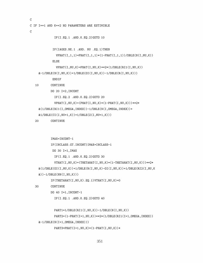
C
C IF I==1 AND K==2 NO PARAMETERS ARE ESTIMIBLE
C
IF(I.EQ.1 .AND.K.EQ.2)GOTO 10
IF(IAGES.NE.1 .AND. NU .EQ.1)THEN
VFHAT(I,1,1)=FHAT(I,1,1)*(1-FHAT(I,1,1))/DBLE(N(I,NU,K))
ELSE
VFHAT(I,NU,K)=FHAT(I,NU,K)**2*(1/DBLE(RI1(I,NU,K))
&-1/DBLE(N(I,NU,K))+1/DBLE(OI(I,NU,K))-1/DBLE(R(I,NU,K)))
ENDIF
10 CONTINUE
DO 20 I=2,INCOHT
IF(I.EQ.2 .AND.K.EQ.2)GOTO 20
VPHAT(I,NU,K)=(PHAT(I,NU,K)*(1-PHAT(I,NU,K)))**2*
&(1/DBLE(RI1(I,OMEGA,INDEX))-1/DBLE(N(I,OMEGA,INDEX))+
&1/DBLE(CI(I,NU+1,K))+1/DBLE(Z(I,NU+1,K)))
20 CONTINUE
IMAX=INCOHT-1
IF(INCLASS.GT.INCOHT)IMAX=INCLASS-1
DO 30 I=1,IMAX
IF(I.EQ.1 .AND.K.EQ.2)GOTO 30
VTHAT(I,NU,K)=(THETAHAT(I,NU,K)*(1-THETAHAT(I,NU,K)))**2*
&(1/DBLE(OI(I,NU,K))+1/DBLE(R(I,NU,K)-OI(I,NU,K))+1/DBLE(RI2(I,NU,K
&))-1/DBLE(NN(I,NU,K)))
IF(THETAHAT(I,NU,K).EQ.1)VTHAT(I,NU,K)=0
30 CONTINUE
DO 40 I=1,INCOHT-1
IF(I.EQ.1 .AND.K.EQ.2)GOTO 40
PART1=1/DBLE(RI1(I,NU,K))-1/DBLE(N(I,NU,K))
PART2=(1-PHAT(I+1,NU,K))**2*(1/DBLE(RI1(I+1,OMEGA,INDEX))
&-1/DBLE(N(I+1,OMEGA,INDEX)))
PART3=PHAT(I+1,NU,K)*(1-PHAT(I,NU,K))*
351

&(N(I+1,OMEGA,INDEX)-RI1(I+1,OMEGA,INDEX))**2/DBLE(N(I+1,OMEGA
&,INDEX)*RI1(I+1,OMEGA,INDEX)*T(I+1,NU+1,K))
PART4=(1-THETAHAT(I,NU,K))**2*(1/DBLE(RI2(I,NU,K))
&-1/DBLE(NN(I,NU,K)))
IF(THETAHAT(I,NU,K).EQ.1)PART4=0.
PART5=THETAHAT(I,NU,K)**2*(NN(I,NU,K)-RI2(I,NU,K))/
&DBLE(NN(I,NU,K))*(1/DBLE(R(I,NU,K)-OI(I,NU,K))-1/DBLE(R(I,NU,K)))
IF(NN(I,NU,K).EQ.0)PART5=0.
VSHAT(I,NU,K)=SHAT(I,NU,K)**2*(PART1+PART2+PART3+PART4
&+PART5)
40 CONTINUE
50 CONTINUE
200 RETURN
END
Subroutine CONSTANT
SUBROUTINE CONSTANT(M,n,nn,RI1,RI2,IAGES,INCOHT,INCLASS,
&IFTRAP,SUM)
C
C RETURNS THE MULTINOMIAL NORMALIZING CONSTANT FOR THE FULL MODEL
C WITH THE DATA IN M-ARRAY FORM RATHER THAN SUMMARIZED AS MSS
C
IMPLICIT DOUBLE PRECISION (A-H,O-Z)
C
C COMPUTES THE RESIDUAL MULTINOMIAL TERM
C FOR THE UNPOOLED LIKELIHOOD
C
INCLUDE ’MPAR’
SUM=0.
DO 50 NU=1,IAGES
DO 50 K=1,IFTRAP+1
DO 25 I=1,INCOHT
TERM1=DLGAMA(DBLE(N(I,NU,K)+1))
DO 15 J=I+1,INCOHT
352

15 TERM1=TERM1-DLGAMA(DBLE(M(I,J,1,1,NU,K)+1))
DO 20 J=I,INCLASS
20 TERM1=TERM1-DLGAMA(DBLE(M(I,J,1,2,NU,K)+1))
TERM1=TERM1-DLGAMA(DBLE(N(I,NU,K)-RI1(I,NU,K)+1))
25 SUM=SUM+TERM1
C
C NOW FOR C(I,2) COHORTS
C
DO 40 I=1,INCLASS-1
TERM2=DLGAMA(DBLE(NN(I,NU,K)+1))
DO 30 J=I+1,INCOHT
30 TERM2=TERM2-DLGAMA(DBLE(M(I,J,2,1,NU,K)+1))
DO 35 J=I+1,INCLASS
35 TERM2=TERM2-DLGAMA(DBLE(M(I,J,2,2,NU,K)+1))
TERM2=TERM2-DLGAMA(DBLE(NN(I,NU,K)-RI2(I,NU,K)+1))
40 SUM=SUM+TERM2
50 CONTINUE
RETURN
END
4. Programme CAPHIS
CAPHIS takes data in capture history format and converts it to the m-array format
currently needed as input to JOLLYOBS. The input file for CAPHIS requires a
capture history for each animal followed by a value for the age of the animal at
first capture. The fictitious animal first captured at age 0 and with capture history
05013 has a line in the CAPHIS input file given by 05013 0 . The final figure
indicates the animal was in age-class 0 when it was first captured in year 2.
Programme CAPHIS FORTRAN code
PROGRAM CAPHIS
C
C THIS PROGRAM READS IN THE DATA IN CAPTURE HISTORY FORMAT AND GENERATES
C THE REDUCED M-ARRAY - AT THE END OF EACH CAPTURE HISTORY THE AGE OF THE
C ANIMAL AT INITIAL CAPTURE NEEDS TO BE PROVIDED
C
353

IMPLICIT DOUBLE PRECISION (A-H,O-Z)
INCLUDE ’C:\JOLLYOBS\MPAR’
PARAMETER(MXRO=4000)
INTEGER CH(MXRO,MXCLAS),TYR,TCLASS(MXRO)
CHARACTER*12 FNAME,FNAME2
1 FORMAT(42I4)
2 FORMAT(20I6)
3 FORMAT(40I1)
4 FORMAT(5I3)
5 FORMAT(A12)
PRINT*,’INPUT FILE NAME ’
READ5,FNAME
PRINT*,’OUTPUT FILE NAME ’
READ5,FNAME2
PRINT*,’NO. CAPTURE PERIODS ’
READ*,INCOHT
PRINT*,’NO. OBSERVATION PERIODS ’
READ*,INCLASS
PRINT*,’NO. AGE CLASSES ’
READ*,IAGES
PRINT*,’TRAP DEPENDENCE? (0 = NO, 1 = YES) ’
READ*,IFTRAP
ICPOOL=0
C
C INITIALIZE DATA ARRAYS
C
DO 20 I=1,INCLASS
DO 20 NU=1,MXCLAS
DO 20 KK=1,2
N(I,NU,KK)=0
354

NN(I,NU,KK)=0
NKILL(I,NU,KK)=0
DO 20 J=1,INCLASS
M(I,J,1,1,NU,KK)=0
M(I,J,1,2,NU,KK)=0
M(I,J,2,1,NU,KK)=0
20 M(I,J,2,2,NU,KK)=0
OPEN(1,FILE=FNAME)
DO 200 L=1,9999
READ(1,1,END=205)(CH(L,J),J=1,INCLASS),JUNK,TCLASS(L)
NU=TCLASS(L)
DO 50 J=1,INCLASS
IF(CH(L,J).NE.0) THEN
TYR=J
GOTO 55
50 ENDIF
55 CONTINUE
C
C ALL ANIMALS ARE FIRST RELEASED AS MEMBERS OF TRAP CLASS 1
C
ISTATUS=1
N(TYR,NU,1)=N(TYR,NU,1)+1
I=TYR
IC=1
IF(CH(L,TYR).EQ.5) THEN
M(TYR,TYR,1,2,NU,1)=M(TYR,TYR,1,2,NU,1)+1
NN(TYR,NU,1)=NN(TYR,NU,1)+1
IC=2
ELSEIF(CH(L,TYR).EQ.6) THEN
M(TYR,TYR,1,2,NU,1)=M(TYR,TYR,1,2,NU,1)+1
ENDIF
C
C ISTATUS REMAINS AT 1 UNTIL THE ANIMAL IS RE-RELEASED
355

C WHEN INCLASS CHANGES TO 2
C
DO 110 J=TYR+1,INCLASS
IF(CH(L,J).EQ.0)GOTO110
IF(CH(L,J).EQ.1)THEN
M(I,J,IC,1,NU,ISTATUS)=M(I,J,IC,1,NU,ISTATUS)+1
ISTATUS=2
NU=TCLASS(L)+J-TYR
IF(NU.GT.4)NU=4
N(J,NU,2)=N(J,NU,2)+1
I=J
IC=1
ELSEIF(CH(L,J).EQ.5) THEN
M(I,J,IC,1,NU,ISTATUS)=M(I,J,IC,1,NU,ISTATUS)+1
ISTATUS=2
NU=TCLASS(L)+J-TYR
IF(NU.GT.4)NU=4
N(J,NU,2)=N(J,NU,2)+1
I=J
IC=1
M(J,J,IC,2,NU,2)=M(J,J,IC,2,NU,2)+1
NN(J,NU,2)=NN(J,NU,2)+1
IC=2
ELSEIF(CH(L,J).EQ.6) THEN
M(I,J,IC,1,NU,ISTATUS)=M(I,J,IC,1,NU,ISTATUS)+1
ISTATUS=2
NU=TCLASS(L)+J-TYR
IF(NU.GT.4)NU=4
N(J,NU,2)=N(J,NU,2)+1
I=J
IC=1
M(J,J,IC,2,NU,2)=M(J,J,IC,2,NU,2)+1
ELSEIF(CH(L,J).EQ.3)THEN
M(I,J,IC,2,NU,ISTATUS)=M(I,J,IC,2,NU,ISTATUS)+1
ISTATUS=2
NU=TCLASS(L)+J-TYR
356

IF(NU.GT.4)NU=4
NN(J,NU,2)=NN(J,NU,2)+1
I=J
IC=2
ELSEIF(CH(L,J).EQ.4) THEN
M(I,J,IC,2,NU,ISTATUS)=M(I,J,IC,2,NU,ISTATUS)+1
ISTATUS=2
ENDIF
110 CONTINUE
200 CONTINUE
205 CONTINUE
CLOSE(1)
OPEN(2,FILE=FNAME2)
WRITE(2,4)INCOHT,INCLASS,IAGES,IFTRAP,ICPOOL
DO 400 NU=1,IAGES
DO 400 KK=1,IFTRAP+1
WRITE(2,2)(N(I,NU,KK),I=1,INCOHT)
WRITE(2,2)(NN(I,NU,KK),I=1,INCLASS-1)
DO 210 I=1,INCOHT
210 WRITE(2,3)(M(I,J,1,1,NU,KK),J=2,INCOHT),
&(M(I,J,1,2,NU,KK),J=1,INCLASS)
IMAX=INCOHT-1
IF(INCLASS.GT.INCOHT)IMAX=INCLASS-1
DO 220 I=1,IMAX
220 WRITE(2,3)(M(I,J,2,1,NU,KK),J=2,INCOHT),
&(M(I,J,2,2,NU,KK),J=1,INCLASS)
400 CONTINUE
CLOSE(2)
END
5. Programmes used in conjunction with SURVIV
Two files facilitate use of programme SURVIV (White 1983) in fitting the models
described in this thesis. The first programme, SVWRITE, takes the input file for
JOLLYOBS and converts it into a SURVIV input file. The second file, ESTANCIL,
357

provides the likelihood function for SURVIV. The compiled code from ESTANCIL
must be saved as EST.OBJ which is then linked with the other SURVIV components
to form a new version of SURVIV incorporating the ESTANCIL likelihood. Before
compiling ESTANCIL.FOR the number of age classes and whether a temporary
trap response is to be fitted must be declared in ESTANCIL.
Programme SVWRITE
PROGRAM SVWRITE
IMPLICIT DOUBLE PRECISION (A-H,O-Z)
INCLUDE ’MPAR’
C
C LOCAL VARIABLES
C
CHARACTER BANNER
CHARACTER*12 FNAME,FNAME2
PRINT*,’INPUT FILE? ’
READ9,FNAME
PRINT*,’OUTPUT FILE? ’
READ9,FNAME2
OPEN(1,FILE=FNAME)
OPEN(2,FILE=FNAME2)
1 FORMAT(5I3)
2 FORMAT(20I6)
3 FORMAT(40I4)
8 FORMAT(A80)
9 FORMAT(A12)
READ(1,8)BANNER
READ(1,1)INCOHT,INCLASS,IAGES,IFTRAP,ICPOOL
DO 20 NU=1,IAGES
DO 20 OMEGA=1,IFTRAP+1
READ(1,2)(N(I,NU,OMEGA),I=1,INCOHT)
READ(1,2)(NN(I,NU,OMEGA),I=1,INCLASS-1)
DO 10 I=1,INCOHT
10 READ(1,3)(M(I,J+1,1,1,NU,OMEGA),J=1,INCOHT-1),
358

& (M(I,J,1,2,NU,OMEGA),J=1,INCLASS)
DO 20 I=1,INCLASS-1
20 READ(1,3)(M(I,J+1,2,1,NU,OMEGA),J=1,INCOHT-1),
& (M(I,J,2,2,NU,OMEGA),J=1,INCLASS)
NPAR=(INCOHT-1)*5+1
IF(INCLASS.GT.INCOHT)NPAR=NPAR+1+(INCLASS-INCOHT)*(1+(INCLASS
-INCOHT-1)/2)
NPAR=IAGES*(IFTRAP+1)*NPAR
WRITE(2,*)’PROC TITLE ;’
4 FORMAT(A16,I3,A1)
5 FORMAT(A7,I5,A1)
6 FORMAT(A2,I3,A2)
7 FORMAT(I3,A2)
WRITE(2,4)’PROC MODEL NPAR=’,NPAR,’;’
DO 50 NU=1,IAGES
DO 50 KK=1,IFTRAP+1
DO 42 I=1,INCOHT
WRITE(2,5)’COHORT:’,N(I,NU,KK),’;’
DO 41 J=I+1,INCOHT
41 WRITE(2,7)M(I,J,1,1,NU,KK),’:;’
DO 42 J=I,INCLASS
42 WRITE(2,7)M(I,J,1,2,NU,KK),’:;’
DO 46 I=1,INCLASS-1
WRITE(2,5)’COHORT:’,NN(I,NU,KK),’;’
DO 45 J=I+1,INCOHT
45 WRITE(2,7)M(I,J,2,1,NU,KK),’:;’
DO 46 J=I+1,INCLASS
46 WRITE(2,7)M(I,J,2,2,NU,KK),’:;’
50 CONTINUE
WRITE(2,*)’PROC ESTIMATE MAXFN=32000 NSIG=6 NOVAR NAME=M1;’
WRITE(2,*)’INITIAL;’
DO 60 I=1,NPAR
60 WRITE(2,6)’S(’,I,’)=’
WRITE(2,*)’PROC STOP;’
END
359

SURVIV subroutine ESTANCIL
SUBROUTINE EST(NP,PPAR,XLL)
C
C Estimation routine for a multi-age study with recaptures
C and resightings
C
IMPLICIT DOUBLE PRECISION (A-H,O-Z)
include ’MODELC’
c
c local parameters
c
PARAMETER (mxage=3,mtrap=2)
C
C LOCAL VARIABLES
C
INTEGER OMEGA
DOUBLE PRECISION F(MAXPAR,mxage,mtrap),S(MAXPAR,mxage,mtrap),
&PP(MAXPAR,mxage,mtrap),
&FF(MAXPAR,mxage,mtrap),THETA(MAXPAR,MXAGE,mtrap),GAMMA,
&PIE(MXCLAS,MAXCHT,MXAGE,mtrap),xi(mxclas,mxage,mtrap),
&zeta(maxcht,mxclas,mxage,mtrap),mu(mxage,2),lam(mxage,2)
&,rho(mxclas,mxage,mtrap)
CALL MOVFLT(PPAR,PAR,NEST)
c
c NB: the data must be arranged in the form: Age-class 0 trap-class 0
c Age-class 0 trap-class 1
c Age-class 1 trap-class 0
c Age-class 2 trap-class 1
c . .
c . .
c . .
c Age-class l trap-class 0
c Age-class l trap-class 1
360

c
c initialise : nch = the number of C(i,1) cohorts
c n1 = the number of years of resighting
c iages = the number of age classes
c IMODEL = 0 permanent emigration model
c = 1 random emigration model
c iftrap = 0 no temporary trap response
c = 1 temporary trap response model
c
nch=4
n1=5
iages=1
iftrap=1
IMODEL=1
nsig=6
small=1.D1**(-NSIG)
c
c initialise the values of rho(i) - the following are for Lake Brunner males
c one age with marking effect
c
rho(1,1,1)=0.0416667
rho(2,1,1)=0.0666667
rho(3,1,1)=0.1052632
rho(4,1,1)=0.3870968
rho(5,1,1)=1.
rho(1,1,2)=small
rho(2,1,2)=small
rho(3,1,2)=0.1666667
rho(4,1,2)=0.1500000
rho(5,1,2)=1.
1 format(5(f8.4))
indx=0
jmp=5*nch-4
if(n1.gt.nch)jmp=jmp+1+(n1-nch)*(1+(n1-nch-1)/2)
do 8 nu=1,iages
361

do 8 kk=1,iftrap+1
it=indx*jump
indx=indx+1
DO 4 I=1,NCH-1
4 PP(I,nu,kk)=SS(I+it)
jump=nch-1
do 5 i=1,nch-1
S(I,nu,kk)=SS(I+jump+it)
FF(I,nu,kk)=SS(I+2*jump+it)
c
c if fitting the markov emigration model assign the first two fidelity
c parameters to mu and lambda - constrain the others to zero
c
if(imodel.eq.3)then
mu(nu,kk)=ss(1+2*jump+it)
lam(nu,kk)=ss(2+2*jump+it)
endif
THETA(I,NU,kk)=SS(I+3*jump+IT)
5 F(I,NU,kk)=SS(I+4*jump+IT)
jump=5*(nch-1)
f(nch,nu,kk)=ss(jump+1+IT)
jump=jump+1
if(n1.eq.nch)goto 8
theta(nch,nu,kk)=ss(jump+1+it)
jump=jump+1
do 6 i=nch+1,n1
k=i-nch
6 xi(i,nu,kk)=ss(jump+k+it)
jump=jump+n1-nch
index=1
do 7 i=nch+1,n1-1
do 7 j=i+1,n1
zeta(i,j,nu,kk)=ss(jump+index+it)
7 index=index+1
ixx=n1-nch
jump=jump+((ixx-1)*ixx)/2
362

8 continue
c do 10 nu=1,iages
c do 10 kk=1,iftrap+1
c do 9 i=1,nch-1
c 9 print1,pp(i,nu,kk),s(i,nu,kk),ff(i,nu,kk),theta(i,nu,kk),
c &f(i,nu,kk)
c print1,f(nch,nu,kk),theta(nch,nu,kk)
c print*,xi(5,nu,kk)
c print*,xi(5,nu,kk),xi(6,nu,kk),xi(7,nu,kk)
c print*,zeta(5,6,nu,kk),zeta(5,7,nu,kk),zeta(6,7,nu,kk)
c 10 print*,’ ’
C
C AIJ = PR(ANIMAL CAPTURED AT I IS NEXT CAPTURED AT J BUT NOT CAPTURED
C BETWEEN I AND J)
C BIJ = PR(ANIMAL CAPTURED AT I NOT IN STUDY AREA AT J AND
C NOT CAPTURED BEFORE J)
C GAMMA(I,J) = PR(ANIMAL LAST CAUGHT AT I IS NOT CAPTURED BY J)
C
k2=iftrap+1
DO 140 NU=1,IAGES
do 140 kk=1,iftrap+1
c
c First compute cell probs for M(i,j,1,1)’s
c
c
c NB to fit the random emigration model use pp(nu) not pp(omega)
C
DO 18 I=kk,NCH
GAMMA=1.
OMEGA=NU+1
IF(NU.EQ.IAGES)OMEGA=IAGES
if(IMODEL.EQ.1)omega=nu
363

IF(I.LE.NCH-1) then
AIJ=FF(I,NU,KK)
BIJ=1-FF(I,NU,KK)
IF(IMODEL.EQ.3) THEN
AIJ=MU(NU,KK)
BIJ=1-MU(NU,KK)
ENDIF
GAMMA=AIJ
ENDIF
ALPHA1=S(I,NU,kk)*THETA(I,NU,kk)*PP(I,OMEGA,kk)
BETA=S(I,NU,kk)*THETA(I,NU,kk)
SUM=ALPHA1*GAMMA
PRD=BETA
PIE(1,I,NU,kk)=SUM
omega=nu+1
if(nu.eq.iages)omega=nu
iom=omega
if(IMODEL.EQ.1)iom=nu
DO 16 J=I+1,NCH-1
K=J-I+1
IK=IFTRAP+1
IF(J.EQ.I+1)IK=KK
c
c update aij and bij and gamma
c
if(imodel.ne.3)then
mu(omega,k2)=ff(J,omega,k2)
lam(omega,k2)=0.
endif
OLDA=AIJ
OLDB=BIJ
AIJ=OLDA*(1-PP(J-1,iOM,ik))*mu(OMEGA,k2)+oldb*lam(omega,k2
&)
BIJ=OLDA*(1-PP(J-1,iOM,ik))*(1-mu(OMEGA,k2)) + OLDB*
364

&(1-lam(omega,k2))
GAMMA=AIJ
iom=iom+1
if(iom.gt.iages)iom=iages
omega=omega+1
if(omega.gt.iages)omega=iages
IT=NU+J-I
IF(IT.GT.IAGES)IT=IAGES
ALPHA1=S(J,IT,k2)*THETA(J,IT,k2)*PP(J,iom,k2)
BETA=S(J,IT,k2)*THETA(J,IT,k2)
PIE(K,I,NU,kk)=PRD*ALPHA1*GAMMA
SUM=SUM+PIE(K,I,NU,kk)
16 PRD=PRD*BETA
c
c compute cell probabilities for M(i,j,1,2)’s
c
ALPHA2=F(I,NU,kk)
PIE(NCH-I+1,I,NU,kk)=ALPHA2
SUM=SUM+alpha2
c
c if i = nch prd and beta must be set to 1
c
beta=1.
prd=1.
gamma=1.
if(i.ne.nch)BETA=S(I,NU,kk)*THETA(I,NU,kk)
if(i.ne.nch)PRD=BETA
IF(I.LE.NCH-1) then
AIJ=FF(I,NU,KK)
BIJ=1-FF(I,NU,KK)
IF(IMODEL.EQ.3) THEN
AIJ=MU(NU,KK)
BIJ=1-MU(NU,KK)
365

ENDIF
ENDIF
omega=nu+1
if(nu.eq.iages)omega=nu
iom=omega
if(IMODEL.EQ.1)iom=nu
it=nu
DO 17 J=I+1,N1
K=(NCH-I) + (J-I+1)
if(j.le.nch)then
ik=iftrap+1
if(j.eq.i+1)ik=kk
GAMMA=AIJ*(1-PP(J-1,iom,ik)) + BIJ
c
c now update aij and bij
c
if(imodel.ne.3)then
mu(omega,k2)=ff(J,omega,k2)
lam(omega,k2)=0.
endif
OLDA=AIJ
OLDB=BIJ
AIJ=OLDA*(1-PP(J-1,iOM,ik))*mu(OMEGA,k2)+oldb*lam(omega,k2
&)
BIJ=OLDA*(1-PP(J-1,iOM,ik))*(1-mu(OMEGA,k2)) + OLDB*
&(1-lam(omega,k2))
iom=iom+1
if(iom.gt.iages)iom=iages
OMEGA=OMEGA+1
IF(OMEGA.GT.IAGES)OMEGA=IAGES
if(it.eq.iages)it=it-1
ALPHA2=F(J,it+1,k2)
366

PIE(K,I,NU,kk)=PRD*ALPHA2*GAMMA
c
c now compute beta(j) and update prd
c
IT=NU+J-I
IF(IT.GT.IAGES)IT=IAGES
c
c only update prd and beta if j < nch, otherwise they will be zero
c
if(j.lt.nch) then
BETA=S(j,IT,k2)*THETA(j,IT,k2)
PRD=PRD*BETA
endif
else
it2=nu+nch-i
if(it2.gt.iages)it2=iages
ik2=iftrap+1
if(i.eq.nch)ik2=kk
PIE(K,I,NU,kk)=PRD*GAMMA*xi(j,it2,ik2)
endif
17 SUM=SUM+PIE(K,I,NU,kk)
18 PIE(NCH-i+n1-i+2,I,NU,kk)=1.-SUM
if(kk.eq.2)PIE(NCH-1+n1-1+2,1,NU,kk)=1.
C
C NOW REPEAT FOR C(I,2) COHORTS
C First for M(i,j,2,1)’s
c
imax=nch-1
if(n1.gt.nch)imax=n1-1
DO 110 I=kk,imax
delta=1.
if(i.gt.nch)goto 95
beta=1.
prd=1.
367

gamma=1.
OMEGA=NU+1
IF(NU.EQ.IAGES)OMEGA=IAGES
if(IMODEL.EQ.1)omega=nu
IF(I.LE.NCH-1)then
AIJ=FF(I,NU,KK)
BIJ=1-FF(I,NU,KK)
IF(IMODEL.EQ.3) THEN
AIJ=MU(NU,KK)
BIJ=1-MU(NU,KK)
ENDIF
GAMMA=AIJ
ENDIF
ALPHA1=S(I,NU,kk)*THETA(I,NU,kk)*PP(I,OMEGA,kk)
if(i.lt.nch)BETA=S(I,NU,kk)*THETA(I,NU,kk)
if(kk.eq.2 .and. i.eq.1)then
delta=0.
else
DELTA=(1-THETA(I,NU,kk))/(THETA(I,NU,kk)*F(I,NU,kk)*
&rho(i,nu,kk))
endif
PRD=BETA
SUM=DELTA*ALPHA1*gamma
PIE(1,nch+I,NU,kk)=SUM
omega=nu+1
if(nu.eq.iages)omega=nu
iom=omega
if(IMODEL.EQ.1)iom=nu
DO 90 J=I+1,NCH-1
K=J-I+1
IK=IFTRAP+1
IF(J.EQ.I+1)IK=KK
368

if(imodel.ne.3)then
mu(omega,k2)=ff(J,omega,k2)
lam(omega,k2)=0.
endif
OLDA=AIJ
OLDB=BIJ
AIJ=OLDA*(1-PP(J-1,iOM,ik))*mu(OMEGA,k2)+oldb*lam(omega,k2)
BIJ=OLDA*(1-PP(J-1,iOM,ik))*(1-mu(OMEGA,k2)) + OLDB*
&(1-lam(omega,k2))
GAMMA=AIJ
iom=iom+1
if(iom.gt.iages)iom=iages
omega=omega+1
if(omega.gt.iages)omega=iages
IT=NU+J-I
IF(IT.GT.IAGES)IT=IAGES
ALPHA1=S(J,IT,k2)*THETA(J,IT,k2)*PP(J,IOM,k2)
BETA=S(J,IT,k2)*THETA(J,IT,k2)
PIE(K,nch+I,NU,kk)=PRD*DELTA*ALPHA1*gamma
SUM=SUM+PIE(K,nch+I,NU,kk)
90 PRD=PRD*BETA
95 continue
c
c compute cell probs for M(i,j,2,2)’s
c
beta=1.
prd=1.
gamma=1.
if(i.gt.nch)goto 105
if(i.lt.nch)BETA=S(I,NU,kk)*THETA(I,NU,kk)
PRD=BETA
IF(I.LE.NCH-1)then
AIJ=FF(I,NU,KK)
369

BIJ=1-FF(I,NU,KK)
IF(IMODEL.EQ.3) THEN
AIJ=MU(NU,KK)
BIJ=1-MU(NU,KK)
ENDIF
GAMMA=AIJ
ENDIF
omega=nu+1
if(nu.eq.iages)omega=nu
iom=omega
if(IMODEL.EQ.1)iom=nu
it=nu
DO 100 J=I+1,N1
K=(NCH-I) + (J-I)
if(j.le.nch)then
ik=iftrap+1
if(j.eq.i+1)ik=kk
GAMMA=AIJ*(1-PP(J-1,iOM,ik)) + BIJ
c
c now update aij and bij
c
if(imodel.ne.3)then
mu(omega,k2)=ff(J,omega,k2)
lam(omega,k2)=0.
endif
OLDA=AIJ
OLDB=BIJ
AIJ=OLDA*(1-PP(J-1,iOM,ik))*mu(OMEGA,k2)+oldb*lam(omega,k2
&)
BIJ=OLDA*(1-PP(J-1,iOM,ik))*(1-mu(OMEGA,k2)) + OLDB*
&(1-lam(omega,k2))
iom=iom+1
if(iom.gt.iages)iom=iages
OMEGA=OMEGA+1
370

IF(OMEGA.GT.IAGES)OMEGA=IAGES
if(it.eq.iages)it=it-1
ALPHA2=F(J,it+1,k2)
PIE(K,nch+I,NU,kk)=PRD*DELTA*ALPHA2*GAMMA
c
c now update beta(j) and prd
c
IT=NU+J-I
IF(IT.GT.IAGES)IT=IAGES
if(j.ne.nch)BETA=S(j,IT,k2)*THETA(j,IT,k2)
if(j.ne.nch)PRD=PRD*BETA
else
it2=nu+nch-i
if(it2.gt.iages)it2=iages
ik2=iftrap+1
if(i.eq.nch)ik2=kk
PIE(K,nch+I,NU,kk)=PRD*delta*GAMMA*xi(j,it2,ik2)
endif
100 SUM=SUM+PIE(K,nch+I,NU,kk)
goto 110
c
c now compute pie(i,j,k,l) for additional C(i,2) cohorts if there are
c observations beyond the final capture period
c
105 continue
sum=0.
do 107 j=i+1,n1
K=J-I
pie(k,nch+i,nu,kk)=zeta(i,j,nu,kk)
107 sum=sum+pie(k,nch+i,nu,kk)
110 PIE(k+1,nch+I,NU,kk)=1.-SUM
if(kk.eq.2)PIE(nch-1+n1,nch+1,NU,kk)=1.
140 CONTINUE
c
c now reshape pie(j,i,nu,k) to p(j,i)
371

c
index=0
do 210 nu=1,iages
do 210 kk=1,iftrap+1
it=index*(nch+n1-1)
index=index+1
do 170 i=1,nch
do 150 k=1,nch-i
150 p(k,i+it)=pie(k,i,nu,kk)
do 160 k=nch-i+1,nch-i+n1-i+1
160 p(k,i+it)=pie(k,i,nu,kk)
170 p(nch-i+n1-i+2,i+it)=pie(nch-i+n1-i+2,i,nu,kk)
do 200 i=1,nch
do 180 k=1,nch-i
180 p(k,nch+i+it)=pie(k,nch+i,nu,kk)
do 190 k=nch-i+1,nch-i+n1-i+1
190 p(k,nch+i+it)=pie(k,nch+i,nu,kk)
200 p(nch-i+n1-i+2,nch+i+it)=pie(nch-i+n1-i+2,nch+i,nu,kk)
do 205 i=nch+1,n1-1
do 202 k=1,n1-nch-i+nch
202 p(k,nch+i+it)=pie(k,nch+i,nu,kk)
205 p(n1-nch-i+nch+1,nch+i+it)=pie(n1-nch-i+nch+1,nch+i,nu,kk)
210 continue
XLL=0.
DO 300 I=1,NCOHT
DO 300 J=1,NCLASS(I)
c print*,i,j,p(j,i),obs(j,i)
300 XLL=XLL-DBLE(OBS(J,I))*LOG(MAX(SMALL,P(J,I)))
Return
end
372